Roweis-Saul classi�er for machine learning

P. Rajamannar? and Gurumurthi V. Ramanan??

AU-KBC Research Centre,MIT Campus of Anna University,

Chromepet, Chennai 600 044, INDIA.

Abstract. In 2000, Saul and Roweis proposed locally linear embeddingas a tool for nonlinear dimensionality reduction [1,2]. In this paper, wemodify the LLE algorithm and formulate it as a classi�er in a mannerreminiscent of He et al [3] and name it after Roweis and Saul. Our ex-periments with the ORL, YALE, FERET face databases and MNISThandwritten database show that our classi�er has recognition rates of95.41%, 95.55%, 95.41% and 92.50% respectively, clearly outperformingthe baseline PCA and LDA classi�ers as well as the recently proposedLaplacianfaces. We propose a modi�cation to the training phase of theclassi�er by perturbing the within class entries of the reconstruction ma-trix constructed during the training phase. This perturbation leads toan increase in the success rates for some datasets. We point out the rela-tionship between the Roweis-Saul classi�er and PCA and LDA. Varioushypothesis tests have been suggested for comparing classi�ers [4,5]. Weapply some of the hypothesis tests suggested by Dietterich and Alpaydinto compare the Roweis-Saul classi�er and the Laplacianfaces and showthat the Roweis-Saul classi�er outperforms the Laplacianfaces for thedatasets considered here.

1 Introduction

The last few years have seen many proposals for non linear dimension reduc-tion such as the ISOMAP, LLE, Laplacian eigenmaps, Hessian eigenmaps andGTM[6,1,2,7,8,9,10]. There are many papers where the authors propose a com-mon framework encompassing these techniques under the ambit of spectral clus-tering [11]. He and Niyogi modi�ed Belkin and Niyogi's Laplacian eigenmapsalgorithm for nonlinear dimensionality reduction into a locality preserving pro-jection [12]. All these techniques addressed the issues of �nding meaningful lowdimensional structures hidden in high dimensional data and analyse the datafrom the point of view of clustering. Recently, He et al. modi�ed Belkin andNiyogi's Laplacian eigenmaps into a classi�er [3,7].

In this paper, we modify the locally linear embedding (LLE) algorithm ofSaul and Roweis in a manner which is reminiscent of He et al.'s modi�cation of? The results of this paper are part of the MS thesis done under the direction of thesecond author. Email:rajamr@au-kbc.org

?? Corresponding author: gurumurthi@au-kbc.org

the Laplacian eigenmaps [3]. In the context of clustering, Belkin and Niyogi intheir landmark paper pointed out that the LLE algorithm of Saul and Roweiswas approximated by Laplacian eigenmaps under certain assumptions [7]. Wefound that these assumptions were far too restrictive even in the context ofclustering. In the case of face recognition and handwritten digits classi�cation,these assumptions are not valid. Our experiments with some well known face andhandwritten digits datasets show that our classi�er outperforms Laplacianfaces.

The paper is organized as follows. Section 2 describes how Saul and Roweis'algorithm can be turned into a classi�er. In Section 3 we analyse the Roweis-Saulclassi�er and indicate the connection with PCA and LDA. Section 4 describesa modi�cation of the training phase of the Roweis-Saul classi�er when the classinformation is available. In Section 5 we measure the recognition rates of theRoweis-Saul classi�er and also compare it with Laplacianfaces, PCA and LDAusing the ORL, YALE, FERET face databases and the MNIST handwrittendigits database. In Section 6, we compare the Roweis-Saul classi�er and Lapla-cianfaces using hypothesis tests. In Section 7, we summarize our results andpoint out some future directions.

2 Turning LLE into Roweis-Saul classi�er

Locally linear embedding (LLE) attempts to compute a low dimensional em-bedding with the property that `nearby points in the high dimensional spaceremain nearby and similarly co-located with respect to one another in the lowdimensional space' [2].

Let x1,x2, · · · ,xN, xi ∈ RD be the feature vectors and X be the D × Nmatrix whose columns are the xi

′s, i.e., X = [x1,x2, · · · ,xN]. The objective ofthe training phase of the Roweis - Saul classi�er is to �nd a smaller dimensiond ¿ D and a D × d transformation V such that Y = VTX, where the neigh-bourhood relations of the yi's which are the columns of Y, is similar to that ofxi's. We call V, the Roweis-Saul transform. During the testing phase, the train-ing vectors as well as the the test vector are projected on this subspace. Thetest vector is then classi�ed on the basis of the euclidean distance or any otherdistance measure to one of the training vectors. In some datasets the numberN of feature vectors is less than the dimension D of each vector. In these cases,it is not computationally feasible to �nd the local coordinates as speci�ed bysteps 1 and 2 of the algorithm given below. Hence, as a preprocessing step, wemay reduce the dimension of the input vectors by principal component analysis(PCA), before proceeding to steps 1 and 2. Steps 1 and 2 coincide with the initialtwo steps of the LLE algorithm [2,1]. We now describe the training phase of theRoweis-Saul classi�er.

2.1 Algorithm for training phase of Roweis-Saul classi�er

Step 0: (optional) Application of PCA: For the sake of notational clarity,assume that the initial feature vectors belong to a D̂ dimensional space. Project

the input points to a subspace along the principal components. Let VPCAbe thetransformation matrix obtained by performing PCA. The dimension of inputpoints will be reduced from D̂ to D, where D ¿ D̂.

Step1: Construction of the neighborhood matrix: Construct a neighbor-hood graph for the N points x1,x2, · · · ,xN. This can be done in any of thefollowing ways.

1. K - nearest neighbors: Construct a graph G over all data points by connectingpoints i and j if i is one of the K nearest neighbors of j.

2. ε - isomap: Construct a graph G over all data points by connecting i and jif they are closer than ε.

3. User de�ned neighbors: Force the neighbors to be the points of the sameclass to which the point belongs. This variation has not been consideredpreviously in the literature [1,2,7]

In the case of segmentation, Shi and Malik, empirically found that one canremove 90 percent of the total connections with each neighborhoods when theneighborhoods are large without a�ecting the eigenvector solution of the system[13].

Step 2: Computation of local linear coordinates: Wij's are chosen so thatthey minimize the reconstruction error

N∑

i

||xi −N∑

j=1

Wijxj||2 (1)

with Wij = 0 if xj 6∈{neighbors of xi} subject to the constraint∑

j Wij = 1∀i.The Wij's are found using the method of of Lagrange multipliers [2].

Let Wi = (Wi1,Wi2, . . . ,WiN) where 1 ≤ i ≤ N. For every �xed i, the La-grange multiplier λ is given by

∂f(Wi1,Wi2, . . . ,WiN)∂Wik

+ λ∂g(Wi1,Wi2, . . . ,WiN)

∂Wik= 0 ∀k = 1,2, ...N

Minimizing the equation (1) is equivalent to solving the above equation bysetting f(Wi1,Wi2, . . . ,WiN) = ||xi −ΣN

j=1Wijxj||2 and g(Wi1,Wi2, . . . ,WiN)= ΣjWij − 1 = 0.

Step 3: Computation of low dimensional embedding: Compute the lowdimensional embedding vectors yi that are best reconstructed by Wij, by mini-mizing the equation

Φ(y) =∑

i

||yi −∑

j

Wijyj||2 (2)

Substituting yi = VTxi, we can rewrite the above equation as

=∑

i

(VTxi −∑

j

WijVTxi)T(VTxi−∑

j

WijVTxi)

In matrix notation the above equation is

Φ(V) = (VTX−VTXW)T(VTX−VTXW) (3)

It is clear that minimizing Φ(V) is equivalent to minimizing the trace of theRHS of the equation (3)

Φ(V) = Trace{(VTX−VTXW)T(VTX−VTXW)

}(4)

We now show how to formulate this minimization as an algebraic eigenvalueproblem. Rewrite the RHS of above equation as follows.

Φ(V) = Trace{VTX(I−W)(I−WT)XTV

}(5)

Let M = X(I−WT)

Φ(V) = Trace{VTMMTV

}(6)

Now minimizing equation (6) is equivalent to the algebraic eigenvalue prob-lem

VTM = λVT (7)The transformation V is found by �rst computing the eigenvectors correspond-ing to (d + 1) smallest eigenvalues of the matrix M. Then the eigenvector corre-sponding to the smallest eigenvalue is discarded since it is zero. The remainingd eigenvectors form the rows of the transformation. We note that this step isdi�erent from the corresponding step in the case of Laplacianfaces [3] where thegeneralized eigenvalue problem is solved.

When we use PCA for reducing the dimension of input data, the Roweis-Saultransform for projecting the feature vectors is given by

V = VPCAV (8)and the low dimensional embedding of the training vectors is given by

Y = VTX (9)

The test vector x̌ is projected using the Roweis-Saul transform V and clas-si�ed as belonging to the same class as yj, using the nearest neighbour rule.

A remark is in order. Belkin and Niyogi showed that the LLE algorithmattempts to minimize fT(I−W)T(I−W)f and under certain conditions, itcan be interpreted as trying to �nd the eigenfunctions of the iterated LaplacianL2, where

(I−W)T(I−W)f ≈ 12L2f .

These conditions imply that pairwise di�erences of the input feature vectorsxi − xj form an orthonormal basis. They also mention in passing that this `isnot usually the case' [7]. This condition is not valid in many supervised learn-ing problems. We emphasize that this condition is not true for all the datasetsconsidered in this paper. This motivated our modi�cation of the LLE algorithminto a classi�er. In the next section, we point out some connections between theRoweis-Saul classi�er and the classical PCA and LDA.

3 Connections between Roweis-Saul classi�er, PCA andLDA

In the training phase of the RS classi�er we minimized the following equation

N∑

i=1

||xi −N∑

j=1

Wijxj||2 (10)

subject to the constraint that∑N

j=1 Wij = 1 ∀i using the method of Lagrangemultipliers.

3.1 Connection with PCA

Let X = (x1,x2, . . . ,xN), where xi ∈ RD and m = 1N

∑Nj=1 xj. If we substitute

Wij = 1N ∀ i, j, in equation (10), it becomes the covariance matrix of the input

data. i.e.,

N∑

i=1

||xi −N∑

j=1

Wijxj||2 =N∑

i=1

(xi −N∑

j=1

Wijxj)T(xi−N∑

j=1

Wijxj)

=N∑

i=1

(xi −XW)T(xi −XW).

Using the fact that XW = m, the RHS of the above equation can be rewrittenas

N∑

i=1

||xi −N∑

j=1

Wijxj||2 =N∑

i=1

(xi −m)T(xi −m) (11)

The technique of PCA involves choosing the eigenvectors corresponding to theleading eigenvalues of the covariance matrix as the basis for projection of theinput data [14,15]. This shows the relationship between Step 2 (�nding locallinear coordinates) of the training phase of the Roweis-Saul classi�er and PCA.During the training phase of the Laplacianfaces, this step is absent because thelinear coordinates are chosen by taking them to be the Euclidean distance or theneighbourhood relationships between the input points [3].

3.2 Connection with LDA

Let C be the number of classes in the given dataset and ci, the number of samplesin each of the class, where 1 ≤ i ≤ C. Let us represent xj and Wjk as xi

j andWi

jk if xj ∈ ci and where 1 ≤ j,k≤ N and mi = 1ci

∑ci

j=1 xij. The equation (10)

can be rewritten as

N∑

i=1

||xi −N∑

j=1

Wijxj||2 =C∑

i=1

ci∑

j=1

||xij−

ci∑

k=1

Wijkx

ik||2

If Wijk = 1

ci∀i, j,k then

∑ci

k=1 Wijkx

ik becomes the class mean of the input

samples (i.e.,) mi

=C∑

i=1

ci∑

j=1

||xij −mi||2

=C∑

i=1

ci∑

j=1

(xij −mi)T(xi

j −mi) (12)

The RHS of equation (12) is the within class scatter matrix SWthat is minimizedin Linear Discriminant Analysis (LDA). In LDA, the denominator of the criterionfunction

J(Wi) =WT

i SBWi

WTi SwWi

(13)

is minimized in order to maximize the criterion function (13) where SB is thebetween class scatter matrix and Swis the within class scatter matrix [15]. Fromthis it is clear that during Step 2, we are minimizing an analogue (equation (10))of the within class scatter matrix in order to �nd the local coordinates.

4 Roweis-Saul with an α perturbation

In this section, we propose a modi�cation of the Roweis-Saul classi�er describedin the previous section. First we assume that the input data consists of a labelled

training set and is ordered using the class information. In Step 3 of trainingphase, described in (2.1), we add a matrix Wα to W, i.e.,

WRSα = Wα + W. (14)We identify the matrix Wα in the above equation (14) with the matrix whoserows and columns are indexed by the input data points. The (i, j)th entry ofWα is α if the ith and the jth points belong to the same class and 1−α if theybelong to di�erent classes. Hence equation (4) becomes

Φ(V) = Trace{VTX(I−WRSα)(I−WT

RSα)XTV}

.

Thereafter, we follow the steps mentioned in (2.1) of the Roweis-Saul trainingphase to compute the embedding. This matrix is motivated by our desire tobring the within class points closer and can be viewed as a perturbation of thereconstruction matrix constructed during Step 3 of the training phase. We chooseα between 1.0 and 0.0, and the typical value used in this paper is 0.9. [Table 2].

Experiments with the databases using the RS classi�er with α graph per-turbation show that it has lower error rate when compared to the RS classi�erand Laplacianfaces. Since this variation makes use of the class information of thedataset, it can be considered as a supervised learning analogue of the Roweis-Saulclassi�er. A similar modi�cation when applied to the Laplacianfaces, also yieldsa similar boost in the performance [Table 2]. This phenomenon is interesting andneeds to be validated for larger and more diverse datasets than considered here.

5 Experiments5.1 Experiments with face databasesThe YALE face database, ORL face database and the FERET database wereused to measure the recognition rates of the Roweis-Saul classi�er and comparedwith the Laplacianfaces [16,17,18]. He et al. had downsampled the images to32 × 32 before performing classi�cation [3]. In our experiments we used threedi�erent image sizes, namely 32× 32, 64× 64 and 128× 128. In the case of theFERET database, we manually selected 106 people each having 4 frontal images.In all these cases we have set the number of neighbors as(K =) 4.

Table 1. Face databases used in the experiments

Database No. of people No. of images per personORL 40 10YALE 15 11FERET 106 4

Table 2. Recognition rates for Roweis-Saul, Laplacianfaces and theirvariations

Dataset Size RS RS α Laplacian Laplacian α PCA LDA

ORL4 training

3264128

95.41% 95.41% 91.66% 92.50% 87.91% 93.33%94.58% 95.41% 91.25% 91.66% 87.08% 92.92%94.58% 95.41% 91.25% 91.66% 87.08% 92.50%

YALE5 training

3264128

95.55% 96.66% 90.00% 94.44% 87.78% 95.56%94.44% 95.55% 88.89% 93.33% 84.44% 94.44%94.44% 95.55% 88.89% 91.11% 84.44% 93.33%

FERET2 training

3264128

95.41% 95.41% 91.66% 92.50% 87.91% 92.22%94.58% 95.41% 91.25% 91.66 87.08% 92.22%92.92% 95.41% 91.25% 91.66 87.08% 92.92%

Fig. 1. Recognition rates for the RS classi�er and Laplacianfaces with increasingnumber of training samples for ORL and YALE databases.

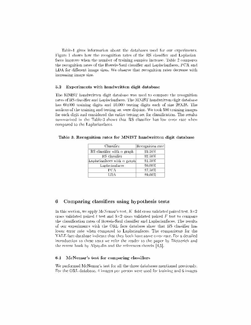
Table-1 gives information about the databases used for our experiments.Figure-1 shows how the recognition rates of the RS classi�er and Laplacian-faces improve when the number of training samples increase. Table-2 comparesthe recognition rates of the Roweis-Saul classi�er and Laplacianfaces, PCA andLDA for di�erent image sizes. We observe that recognition rates decrease withincreasing image size.

5.2 Experiments with handwritten digit database

The MNIST handwritten digit database was used to compare the recognitionrates of RS classi�er and Laplacianfaces. The MNIST handwritten digit databasehas 60,000 training digits and 10,000 testing digits each of size 28X28. Theauthors of the training and testing set were disjoint. We took 500 training imagesfor each digit and considered the entire testing set for classi�cation. The resultssummarized in the Table-3 shows that RS classi�er has low error rate whencompared to the Laplacianfaces.

Table 3. Recognition rates for MNIST handwritten digit database

Classi�er Recognition rateRS classi�er with α graph 93.50%

RS classi�er 92.50%Laplacianfaces with α graph 91.50%

Laplacianfaces 90.00%PCA 87.50%LDA 89.00%

6 Comparing classi�ers using hypothesis tests

In this section, we apply McNemar's test, K- fold cross validated paired test, 5×2cross validated paired t test and 5×2 cross validated paired F test to comparethe classi�cation rates of Roweis-Saul classi�er and Laplacianfaces. The resultsof our experiments with the ORL face database show that RS classi�er haslower error rate when compared to Laplacianfaces. The comparisons for theYALE face database indicate that they both have same error rate. For a detailedintroduction to these tests we refer the reader to the paper by Dietterich andthe recent book by Alpaydin and the references therein [4,5].

6.1 McNemar's test for comparing classi�ers

We performed McNemar's test for all the three databases mentioned previously.For the ORL database, 4 images per person were used for training and 6 images

per person for testing. The YALE database was tested with 5 images per personin training and the remaining for testing. The FERET database was tested using2 images per person for training and the remaining 2 images for testing. Thistest takes into account the number of samples misclassi�ed by the Laplacianfaceswhen compared to the Roweis-Saul classi�er and vice-versa. The null hypothesis(H0) is that both the classi�ers have equal error rate i.e. e01 = e10.

e00 : No. of samples misclassi�ed by both classi�erse01 : No. of samples misclassi�ed by Laplacianfaces but not Roweis-Saul classi�ere10 : No. of samples misclassi�ed by Roweis-Saul classi�er but not Laplacianfacese11 : No. of samples correctly classi�ed by both classi�ers

The values of eij's and the results are available in Table-4. We have the chi-square statistic with one degree of freedom χ2 = (|e01−e10|−1)2

e01+e10. McNemar's test

accepts the null hypothesis at signi�cance level α if χ2 ≤ χ2α,1. The typical value

for α is 0.05 and χ20.05,1 = 3.84. Since the null hypothesis is rejected and e01 is

greater than e10 for ORL and FERET database, we conclude that the Roweis-Saul classi�er outperforms the Laplacianfaces for these databases. Even thoughe01 is greater than e10 for the Yale database, the χ2 value is in the acceptablerange. Hence, we conclude that both the classi�ers have same error rate. Theresults of McNemar's test are shown in Table-4.

Table 4. Results of McNemar's testDatabase e00 e01 e10 e11 χ Null hypothesisORL 11 8 2 219 4.9 REJECT

FERET 14 9 1 188 5.6 REJECTYale 4 5 1 80 1.5 ACCEPT

6.2 K - fold cross validated paired t test

In the K-fold cross validated paired test the dataset is divided randomly into Kequal parts [5]. To get the training and testing set, we combine K − 1 parts toform the training set and the remaining part for testing. In the subsequent round,we take another one of K parts for testing and combine the remaining K−1 partsfor training. We perform this experiment till all the K parts have been tested.We record the error rates p1

i for the �rst classi�er and p2i for the second classi�er,

where 1 ≤ i ≤ K and calculate the di�erence in error rates pi = p1i − p2

i . Thenull hypothesis H0 assumed here is that mean µ of the distribution of di�erencein error rates is zero. We perform a t test to check whether the mean of thedistribution of di�erence in error rates falls in the acceptable range. If it doesnot fall in the acceptable range, we reject the null hypothesis. The t test statistic

with K−1 degrees of freedom is given by tK−1 =√

KmS , where m =

PKi=1 pi

K andS =

PKi=1(pi−m)2

K−1 .

The K-fold cross validated paired t test accepts the null hypothesis thatboth the classi�ers have same error rate at signi�cance level α if tK−1 is in theinterval (−tα/2,K−1, tα/2,K−1). If tK−1 < −tα/2,K−1, the �rst classi�er has ahigher error rate when compared to the second classi�er. If tK−1 > tα/2,K−1,the second classi�er has a higher error rate when compared to the �rst one.

The results of this test for the ORL and YALE face datasets are summarizedin Table-5. Since the null hypothesis is rejected for ORL database and it exceedstα/2,K−1, we conclude that Laplacianfaces has a higher error rate when comparedto RS classi�er. Since the tK−1value of YALE database is in the acceptablerange, we accept the null hypothesis and conclude that both Laplacianfaces andRS classi�er have the same error rates.

Table 5. K - fold cv paired t test with K = 10 & α = 0.05

Database −tα/2,K−1 tK−1 tα/2,K−1 Null HypothesisORL -2.26 2.5038 2.26 REJECTYALE -2.26 1.0437 2.26 ACCEPT

6.3 5×2 cross validated paired t test

In 5×2 cv paired t test proposed by Dietterich, we divide the dataset randomlyinto two equal parts, to get the �rst pair of training and testing set [4]. Then weswap the role of training and testing sets. To get the second pair we shu�e thedataset and again divide it randomly into two equal parts. We repeat this forthree more pairs, and get ten training and testing sets. In all, we perform �vereplications of twofold cross-validation. Even though it is possible to get moretraining and testing pairs, Dietterich points out that after �ve folds, the trainingand testing sets overlap and the error rates calculated becomes dependent [4].

Let p(j)i be the di�erence between the error rates of the two classi�ers on the

fold j = 1, 2 of replication i = 1, . . . , 5. Let the average on the replication i bepi = (p(1)

i + p(2)i )/2, and the variance be s2

i = (p(1)i − pi)2/(p(2)

i − pi)2.The null hypothesis is that the two classi�cation algorithms have the same

error rate p(j)i . Here p

(j)i can be treated as approximately normal distributed

with 0 mean and unknown variance σ2. Then p(j)i /σ is approximately unit nor-

mal. If we assume p(1)i and p

(2)i are independent normals, then s2

i /σ2 has a χ2

distribution with one degree of freedom. If each of s2i are independent, then their

sum is χ2 with �ve degrees of freedom.M =

P5i=1 s2

i

σ2 ∼ χ25 and

t =p(1)1√M/5

=p(1)1√∑5

i=1 s2i /5

∼ t5 (15)

The above equation is a t statistic with �ve degrees of freedom. We accept thenull hypothesis that both the classi�ers have the same error rate at signi�cancelevel α if this value is in the interval (−tα/2,5, tα/2,5). t0.025,5 = 2.57. Since the tvalue for ORL face database is not in the acceptable range, the null hypothesis isrejected and we conclude that Laplacianfaces has more error rate when comparedto RS classi�er. Since the t value of YALE database is in the acceptable rangewe accept the null hypothesis and conclude that both Laplacianfaces and RSclassi�er have same error rates. The results are summarized in Table-6.

Table 6. 5×2 cv paired t test with α = 0.05

Database ORL YALEp1

p2

p3

p4

p5

5.002.252.756.253.25

1.332.331.002.004.00

s21

s22

s23

s24

s25

0.50003.31253.1253.1251.125

0.87120.21782.00000.87128.0000

t 3.6770 1.2932t0.025,5 2.57 2.57

Null Hypothesis REJECT ACCEPT

6.4 5×2 cross validated paired F test

The numerator in equation (15) is arbitrary and can take ten di�erent valuesnamely p

(j)i , j = 1, 2, i = 1, . . . , 5 and thus we get ten di�erent t statistics.

t(j)i =

p(j)i√∑5

i=1 s2i /5

Alpaydin proposed an extension to the 5×2 cross validated t test by consid-ering the ten possible statistics. If p

(j)i /σ ∼ Z, then (p(j)

i )2/σ2 ∼ χ2 and theirsum is chi-square with ten degrees of freedom.

N =

∑5i=1

∑2j=1(p

(j)i )2

σ2= χ2

10

If we replace the numerator of equation (15) by the above equation, the resultingstatistic is the ratio of two chi-square distributed random variables. Alpaydinnotes that 'two such variables divided by their corresponding degrees of freedomis F distributed with ten and �ve degrees of freedom' [5].

f =N/10M/5

=

∑5i=1

∑2j=1(p

(j)i )2

2∑5

i=1 s2i

∼ F10,5

This test accepts the null hypothesis that both the classi�ers have the same errorrate for a signi�cance level α if the value is less than Fα,10,5. F0.05,10,5 = 4.74.

Since the f value of ORL face database is not less than Fα,10,5, we reject thenull hypothesis and we conclude that Laplacianfaces has more error rate whencompared to RS classi�er for ORL. Since the f value of YALE database is lessthan Fα,10,5, we accept the null hypothesis and conclude that both Laplacianfacesand RS classi�er has same error rates for YALE face database. The results aresummarized in Table-7.

Table 7. 5×2 cv paired F test α = 0.05

Database N M f Fα,10,5 Null HypothesisORL 188.50 11.5625 8.4246 4.74 REJECTYALE 68.3824 11.9602 2.8587 4.74 ACCEPT

7 Conclusion

We modi�ed the LLE algorithm for nonlinear dimensionality reduction and for-mulated it as a classi�er. We measured the performance of this classi�er usingthe ORL, YALE and FERET face databases and the MNIST handwritten digitdatabase against classi�ers such as PCA, LDA and the related Laplacianfacesand found that it outperformed them. We also indicated the relationships be-tween the Roweis-Saul classi�er and PCA and LDA. We modi�ed the trainingphase of the classi�er by perturbing the within class entries of the reconstructionmatrix constructed during the training phase. We proved that this perturbationleads to a small increase in the success rates for some datasets. We used the hy-pothesis tests suggested by Dietterich and Alpaydin to compare the Roweis-Saulclassi�er and the Laplacianfaces. The results from these tests seem to indicatethat Roweis-Saul performs better than the Laplacianfaces for most cases consid-ered in this paper. Since the datasets considered in this paper consist of images,

the results of this paper need to be validated for more diverse datasets. Classi�erssuch as PCA have been viewed from other perspectives such as reconstruction,compression and ease of computation. Bengio et al touch upon some compu-tational issues as well as a generalized framework in the case of LLE [11]. Asimilar understanding of the Roweis-Saul classi�er and its variation is requiredfor applying it to larger and more diverse datasets.

References1. Saul, L.K., Roweis, S.T.: Think globally, �t locally: Unsupervised learning of low

dimensional manifold. Journal of Machine Learning Research 4 (2003) 119�1552. Roweis, S., Saul, L.: Nonlinear dimensionality reduction by local linear embedding.

Science 290 (2000) 2323�23263. He, X., Yan, S., Hu, Y., Niyogi, P., Zhang, H.: Face recognition using Laplacian-

faces. IEEE Trans. Pattern Anal. Mach. Intell. 27 (2005) 1�134. Dietterich, T.G.: Approximate statistical test for comparing supervised classi�ca-

tion learning algorithms. Neural Computation 10 (1998) 1895�19235. Alpaydin, E.: Introduction to Machine Learning. The MIT Press (2004)6. Tenenbaum, J., Desilva, V., Langford, J.: A global geometric framework for non-

linear dimensionality reduction. Science 290 (2000) 2319�23237. Belkin, M., Niyogi, P.: Laplacian eigenmaps for dimensionality reduction and data

representation. Neural Comput. 15 (2003) 1373�13968. Belkin, M., Niyogi, P.: Laplacian eigenmaps and spectral techniques for embedding

and clustering. In Dietterich, T.G., Becker, S., Ghahramani, Z., eds.: Advances inNeural Information Processing Systems 14, Cambridge, MA, MIT Press (2002)

9. Donoho, D., Grimes, C.: Hessian eigenmaps: new locally linear embedding tech-niques for highdimensional data. (2003)

10. Bishop, C.M., Svensen, M., Williams, C.K.I.: GTM: The generative topographicmapping. Neural Computation 10 (1998) 215�234

11. Bengio, Y., Paiement, J., Vincent, P., Delalleau, O., Le Roux, N., Ouimet, M.: Out-of-sample extensions for LLE, isomap, MDS, eigenmaps, and spectral clustering.(2004)

12. He, X., Niyogi, P.: Locality preserving projections (2002)13. Shi, J., Malik, J.: Normalized cuts and image segmentation. IEEE Trans. Pattern

Anal. Mach. Intell. 22 (2000) 888�90514. Turk, M., Pentland, A.: Eigenfaces for recognition. Journal of Cognitive Neuro-

science 3 (1991) 71�8615. Duda, R.O., E.Hart, P., Stork, D.G.: Pattern Classi�cation. John Wiley Sons, Inc

(2002)16. Yale University: (YALE face database)17. AT&TLaboratories: (ORL face database)18. Phillips, P., Wechsler, H., Huang, J., Rauss, P.: The FERET database and evalu-

ation procedure for face recognition algorithms. Image Vision Comput. 16 (1998)295�306