Measuring Generalization and Overfitting in Machine Learning
171
Measuring Generalization and Overfitting in Machine Learning Rebecca Roelofs Electrical Engineering and Computer Sciences University of California at Berkeley Technical Report No. UCB/EECS-2019-102 http://www2.eecs.berkeley.edu/Pubs/TechRpts/2019/EECS-2019-102.html June 19, 2019
-
Upload
khangminh22 -
Category
Documents
-
view
6 -
download
0
Transcript of Measuring Generalization and Overfitting in Machine Learning

Measuring Generalization and Overfitting in MachineLearning
Rebecca Roelofs
Electrical Engineering and Computer SciencesUniversity of California at Berkeley
Technical Report No. UCB/EECS-2019-102http://www2.eecs.berkeley.edu/Pubs/TechRpts/2019/EECS-2019-102.html
June 19, 2019

Copyright © 2019, by the author(s).All rights reserved.
Permission to make digital or hard copies of all or part of this work forpersonal or classroom use is granted without fee provided that copies arenot made or distributed for profit or commercial advantage and that copiesbear this notice and the full citation on the first page. To copy otherwise, torepublish, to post on servers or to redistribute to lists, requires prior specificpermission.

Measuring Generalization and Overfitting in Machine Learning
by
Rebecca Roelofs
A dissertation submitted in partial satisfaction of the
requirements for the degree of
Doctor of Philosophy
in
Computer Science
in the
Graduate Division
of the
University of California, Berkeley
Committee in charge:
Professor Benjamin Recht, Co-chairProfessor James Demmel, Co-chairAssociate Professor Moritz Hardt
Professor Bruno Olshausen
Summer 2019

Measuring Generalization and Overfitting in Machine Learning
Copyright 2019by
Rebecca Roelofs

1
Abstract
Measuring Generalization and Overfitting in Machine Learning
by
Rebecca Roelofs
Doctor of Philosophy in Computer Science
University of California, Berkeley
Professor Benjamin Recht, Co-chair
Professor James Demmel, Co-chair
Due to the prevalence of machine learning algorithms and the potential for their decisionsto profoundly impact billions of human lives, it is crucial that they are robust, reliable, andunderstandable. This thesis examines key theoretical pillars of machine learning surroundinggeneralization and overfitting, and tests the extent to which empirical behavior matchesexisting theory. We develop novel methods for measuring overfitting and generalization,and we characterize how reproducible observed behavior is across differences in optimizationalgorithm, dataset, task, evaluation metric, and domain.
First, we examine how optimization algorithms bias machine learning models towardssolutions with varying generalization properties. We show that adaptive gradient methodsempirically find solutions with inferior generalization behavior compared to those found bystochastic gradient descent. We then construct an example using a simple overparameterizedmodel that corroborates the algorithms’ empirical behavior on neural networks.
Next, we study the extent to which machine learning models have overfit to commonlyreused datasets in both academic benchmarks and machine learning competitions. We buildnew test sets for the CIFAR-10 and ImageNet datasets and evaluate a broad range of clas-sification models on the new datasets. All models experience a drop in accuracy, whichindicates that current accuracy numbers are susceptible to even minute natural variations inthe data distribution. Surprisingly, despite several years of adaptively selecting the modelsto perform well on these competitive benchmarks, we find no evidence of overfitting. Wethen analyze data from the machine learning platform Kaggle and find little evidence ofsubstantial overfitting in ML competitions. These findings speak to the robustness of theholdout method across different data domains, loss functions, model classes, and humananalysts.
Overall, our work suggests that the true concern for robust machine learning is distribu-tion shift rather than overfitting, and designing models that still work reliably in dynamicenvironments is a challenging but necessary undertaking.

i
To my family

ii
Contents
Contents iv
List of Figures v
List of Tables viii
1 Introduction 11.1 Formal background on generalization and overfitting . . . . . . . . . . . . . . 2
1.1.1 Generalization error . . . . . . . . . . . . . . . . . . . . . . . . . . . 31.1.2 Adaptive overfitting . . . . . . . . . . . . . . . . . . . . . . . . . . . . 4
1.2 Dissertation overview . . . . . . . . . . . . . . . . . . . . . . . . . . . . . . . 4
2 Generalization properties of adaptive gradient methods 62.1 Introduction . . . . . . . . . . . . . . . . . . . . . . . . . . . . . . . . . . . . 62.2 Background . . . . . . . . . . . . . . . . . . . . . . . . . . . . . . . . . . . . 7
2.2.1 Related work . . . . . . . . . . . . . . . . . . . . . . . . . . . . . . . 82.3 The perils of preconditioning . . . . . . . . . . . . . . . . . . . . . . . . . . . 9
2.3.1 Non-adaptive methods . . . . . . . . . . . . . . . . . . . . . . . . . . 92.3.2 Adaptive methods . . . . . . . . . . . . . . . . . . . . . . . . . . . . . 92.3.3 Adaptivity can overfit . . . . . . . . . . . . . . . . . . . . . . . . . . 112.3.4 Why SGD converges to the minimum norm solution . . . . . . . . . . 12
2.4 Deep learning experiments . . . . . . . . . . . . . . . . . . . . . . . . . . . . 132.4.1 Hyperparameter tuning . . . . . . . . . . . . . . . . . . . . . . . . . . 142.4.2 Convolutional neural network . . . . . . . . . . . . . . . . . . . . . . 142.4.3 Character-Level language modeling . . . . . . . . . . . . . . . . . . . 152.4.4 Constituency parsing . . . . . . . . . . . . . . . . . . . . . . . . . . . 16
2.5 Conclusion . . . . . . . . . . . . . . . . . . . . . . . . . . . . . . . . . . . . . 172.6 Supplementary material . . . . . . . . . . . . . . . . . . . . . . . . . . . . . 19
2.6.1 Differences between Torch, DyNet, and Tensorflow . . . . . . . . . . . 192.6.2 Step sizes used for parameter tuning . . . . . . . . . . . . . . . . . . 19
3 Do ImageNet classifiers generalize to ImageNet? 21

iii
3.1 Introduction . . . . . . . . . . . . . . . . . . . . . . . . . . . . . . . . . . . . 213.2 Potential causes of accuracy drops . . . . . . . . . . . . . . . . . . . . . . . . 22
3.2.1 Distinguishing between the two mechanisms . . . . . . . . . . . . . . 243.3 Summary of our experiments . . . . . . . . . . . . . . . . . . . . . . . . . . . 25
3.3.1 Choice of datasets . . . . . . . . . . . . . . . . . . . . . . . . . . . . 253.3.2 Dataset creation methodology . . . . . . . . . . . . . . . . . . . . . . 253.3.3 Results on the new test sets . . . . . . . . . . . . . . . . . . . . . . . 273.3.4 Experiments to test follow-up hypotheses . . . . . . . . . . . . . . . . 29
3.4 Understanding the impact of data cleaning on ImageNet . . . . . . . . . . . 293.5 CIFAR-10 experiment details . . . . . . . . . . . . . . . . . . . . . . . . . . 33
3.5.1 Dataset creation methodology . . . . . . . . . . . . . . . . . . . . . . 343.5.2 Follow-up hypotheses . . . . . . . . . . . . . . . . . . . . . . . . . . . 36
3.6 ImageNet experiment details . . . . . . . . . . . . . . . . . . . . . . . . . . . 423.6.1 Dataset creation methodology . . . . . . . . . . . . . . . . . . . . . . 433.6.2 Model performance results . . . . . . . . . . . . . . . . . . . . . . . . 513.6.3 Follow-up hypotheses . . . . . . . . . . . . . . . . . . . . . . . . . . . 52
3.7 Discussion . . . . . . . . . . . . . . . . . . . . . . . . . . . . . . . . . . . . . 593.7.1 Adaptivity gap . . . . . . . . . . . . . . . . . . . . . . . . . . . . . . 593.7.2 Distribution gap . . . . . . . . . . . . . . . . . . . . . . . . . . . . . 603.7.3 A model for the linear fit . . . . . . . . . . . . . . . . . . . . . . . . . 60
3.8 Related work . . . . . . . . . . . . . . . . . . . . . . . . . . . . . . . . . . . 623.9 Conclusion and future work . . . . . . . . . . . . . . . . . . . . . . . . . . . 633.10 Supplementary material for CIFAR-10 . . . . . . . . . . . . . . . . . . . . . 643.11 Supplementary material for ImageNet . . . . . . . . . . . . . . . . . . . . . . 73
4 A meta-analysis of overfitting in machine learning 984.1 Introduction . . . . . . . . . . . . . . . . . . . . . . . . . . . . . . . . . . . . 984.2 Background and setup . . . . . . . . . . . . . . . . . . . . . . . . . . . . . . 99
4.2.1 Adaptive overfitting . . . . . . . . . . . . . . . . . . . . . . . . . . . . 994.2.2 Kaggle . . . . . . . . . . . . . . . . . . . . . . . . . . . . . . . . . . . 100
4.3 Overview of Kaggle competitions and our resulting selection criteria . . . . . 1014.4 Detailed analysis of competitions scored with classification accuracy . . . . . 102
4.4.1 First analysis level: visualizing the overall trend . . . . . . . . . . . . 1034.4.2 Second analysis level: zooming in to the top submissions . . . . . . . 1044.4.3 Third analysis level: quantifying the amount of random variation . . 1054.4.4 Computation of p-values . . . . . . . . . . . . . . . . . . . . . . . . . 1074.4.5 Aggregate view of the accuracy competitions . . . . . . . . . . . . . . 1084.4.6 Did we observe overfitting? . . . . . . . . . . . . . . . . . . . . . . . . 109
4.5 Classification competitions with further evaluation metrics . . . . . . . . . . 1094.6 Related work . . . . . . . . . . . . . . . . . . . . . . . . . . . . . . . . . . . 1104.7 Conclusion and future work . . . . . . . . . . . . . . . . . . . . . . . . . . . 1114.8 Supplementary material . . . . . . . . . . . . . . . . . . . . . . . . . . . . . 112

iv
4.8.1 Accuracy . . . . . . . . . . . . . . . . . . . . . . . . . . . . . . . . . . 1124.8.2 AUC . . . . . . . . . . . . . . . . . . . . . . . . . . . . . . . . . . . . 1254.8.3 Map@K . . . . . . . . . . . . . . . . . . . . . . . . . . . . . . . . . . 1354.8.4 MulticlassLoss . . . . . . . . . . . . . . . . . . . . . . . . . . . . . . . 1384.8.5 LogLoss . . . . . . . . . . . . . . . . . . . . . . . . . . . . . . . . . . 1424.8.6 Mean score differences over time . . . . . . . . . . . . . . . . . . . . . 145
5 Conclusion 1465.1 Future Work . . . . . . . . . . . . . . . . . . . . . . . . . . . . . . . . . . . . 146
Bibliography 149
v
List of Figures
2.1 Training and test errors of various optimization algorithms on CIFAR-10. . . . . 152.2 Performance curves on the training data and the development/test data for three
natural language tasks. . . . . . . . . . . . . . . . . . . . . . . . . . . . . . . . . 18
3.1 Model accuracy on the original CIFAR-10 and ImageNet test sets vs. our newtest sets. . . . . . . . . . . . . . . . . . . . . . . . . . . . . . . . . . . . . . . . . 22
3.2 Model accuracy on the original ImageNet validation set vs. accuracy on two vari-ants of our new test set. We refer the reader to Section 3.4 for a description ofthese test sets. Each data point corresponds to one model in our testbed (shownwith 95% Clopper-Pearson confidence intervals). On Threshold0.7, the model ac-curacies are 3% lower than on the original test set. On TopImages, which containsthe images most frequently selected by MTurk workers, the models perform 2%better than on the original test set. The accuracies on both datasets closely fol-low a linear function, similar to MatchedFrequency in Figure 3.1. The red shadedregion is a 95% confidence region for the linear fit from 100,000 bootstrap samples. 32
3.3 Randomly selected images from the original and new CIFAR-10 test sets. . . . . 363.4 The pipeline for creating the new ImageNet test set. . . . . . . . . . . . . . . . 443.5 The user interface employed in the original ImageNet collection process for the
labeling tasks on Amazon Mechanical Turk. . . . . . . . . . . . . . . . . . . . . 473.6 Our user interface for labeling tasks on Amazon Mechanical Turk. . . . . . . . . 483.7 The user interface we built to review dataset revisions and remove incorrect or
near duplicate images. . . . . . . . . . . . . . . . . . . . . . . . . . . . . . . . . 553.8 Probit versus linear scaling for model accuracy comparisons. . . . . . . . . . . . 563.9 Impact of the reviewing passes on the accuracy of a resnet152 on our new
MatchedFrequency test set. . . . . . . . . . . . . . . . . . . . . . . . . . . . . . . 573.10 Model accuracy on the original ImageNet validation set vs. accuracy on the first
revision of our MatchedFrequency test set. . . . . . . . . . . . . . . . . . . . . . 583.11 Hard images from our new test set that no model correctly. The caption of
each image states the correct class label (“True”) and the label predicted by mostmodels (“Predicted”). . . . . . . . . . . . . . . . . . . . . . . . . . . . . . . . . . 70
3.12 Model accuracy on the original ImageNet validation set vs. each of our new testsets using linear scale. . . . . . . . . . . . . . . . . . . . . . . . . . . . . . . . . 91

vi
3.13 Model accuracy on the original ImageNet validation set vs. our new test sets usingprobit scale. . . . . . . . . . . . . . . . . . . . . . . . . . . . . . . . . . . . . . . 92
3.14 Randomly selected images from the original ImageNet validation set and our newImageNet test sets. . . . . . . . . . . . . . . . . . . . . . . . . . . . . . . . . . . 93
3.15 Model accuracy on the new test set stratified by selection frequency bin. . . . . 943.16 Model accuracy on the original test set stratified by selection frequency bin. . . 953.17 Stratified model accuracies on the original ImageNet validation set versus accu-
racy on our new test set MatchedFrequency . . . . . . . . . . . . . . . . . . . . . 963.18 Random images from the original ImageNet validation set for three pairs of classes with
ambiguous class boundaries. . . . . . . . . . . . . . . . . . . . . . . . . . . . . . . 97
4.1 Overview of the Kaggle competitions. The left plot shows the distribution ofsubmissions per competition. The right plot shows the score types that are mostcommon among the competitions with at least 1,000 submissions. . . . . . . . . 101
4.2 Private versus public accuracy for all submissions for the most popular Kaggleaccuracy competitions. . . . . . . . . . . . . . . . . . . . . . . . . . . . . . . . 104
4.3 Private versus public accuracy for the top 10% of submissions for the most popularKaggle accuracy competitions. . . . . . . . . . . . . . . . . . . . . . . . . . . . . 105
4.4 Empirical CDFs of the p-values for three (sub)sets of submissions in the fouraccuracy competitions with the largest number of submissions. . . . . . . . . . . 106
4.5 Empirical CDF of the mean accuracy differences for Kaggle accuracy competitionsand mean accuracy difference vs. competition end date. . . . . . . . . . . . . . . 108
4.6 Empirical CDF of mean score differences for 40 AUC competitions, 12 MAP@Kcompetitions, 15 LogLoss competitions, and 11 MulticlassLoss competitions. . . 110
4.7 Mean accuracy difference outlier competitions . . . . . . . . . . . . . . . . . . . 1154.8 Private versus public accuracy for all submissions for the most popular Kaggle
accuracy competitions. . . . . . . . . . . . . . . . . . . . . . . . . . . . . . . . 1174.8 Private versus public accuracy for all submissions for the most popular Kaggle
accuracy competitions. . . . . . . . . . . . . . . . . . . . . . . . . . . . . . . . 1184.9 Private versus public accuracy for top 10% of submissions for the most popular
Kaggle accuracy competitions. . . . . . . . . . . . . . . . . . . . . . . . . . . . . 1204.9 Private versus public accuracy for all submissions for the most popular Kaggle
accuracy competitions. . . . . . . . . . . . . . . . . . . . . . . . . . . . . . . . 1214.10 Competitions whose empirical CDFs agree with the idealized null model that
assumes no overfitting . . . . . . . . . . . . . . . . . . . . . . . . . . . . . . . . 1224.11 Empirical CDFs for an idealized null model that assumes no overfitting for all
Kaggle accuracy competitions. . . . . . . . . . . . . . . . . . . . . . . . . . . . . 1234.11 Empirical CDFs for an idealized null model that assumes no overfitting for all
Kaggle accuracy competitions. . . . . . . . . . . . . . . . . . . . . . . . . . . . . 1244.12 Private versus public AUC for all submissions for Kaggle AUC competitions. . 1304.12 Private versus public AUC for all submissions for Kaggle AUC competitions. . . 131

vii
4.13 Private versus public accuracy for top 10% of submissions for Kaggle AUC com-petitions. . . . . . . . . . . . . . . . . . . . . . . . . . . . . . . . . . . . . . . . 133
4.13 Private versus public AUC for top 10% of submissions for Kaggle AUC competitions.1344.14 Private versus public MAP@K for all submissions for Kaggle MAP@K competitions.1364.15 Private versus public MAP@K for top 10% of submissions for Kaggle MAP@K
competitions. . . . . . . . . . . . . . . . . . . . . . . . . . . . . . . . . . . . . . 1374.16 Private versus public MulticlassLoss for all submissions for Kaggle MulticlassLoss
competitions. . . . . . . . . . . . . . . . . . . . . . . . . . . . . . . . . . . . . . 1404.17 Private versus public MulticlassLoss for top 10% of submissions for Kaggle Mul-
ticlassLoss competitions. . . . . . . . . . . . . . . . . . . . . . . . . . . . . . . . 1414.18 Private versus public LogLoss for all submissions for Kaggle LogLoss competitions.1434.19 Private versus public LogLoss for top 10% of submissions for Kaggle LogLoss
competitions. . . . . . . . . . . . . . . . . . . . . . . . . . . . . . . . . . . . . . 1444.20 Mean score differences versus competition end date for all classification evaluation
metrics. . . . . . . . . . . . . . . . . . . . . . . . . . . . . . . . . . . . . . . . . 145

viii
List of Tables
2.1 Parameter settings of optimization algorithms used in deep learning. . . . . . . 82.2 Summary of the model architectures, datasets, and frameworks used in deep
learning experiments. . . . . . . . . . . . . . . . . . . . . . . . . . . . . . . . . . 132.3 Default hyperparameters for algorithms in deep learning frameworks. . . . . . . 19
3.1 Model accuracies on the original CIFAR-10 test set, the original ImageNet vali-dation set, and our new test set. . . . . . . . . . . . . . . . . . . . . . . . . . . . 27
3.2 Impact of the three sampling strategies for our ImageNet test sets. . . . . . . . . 313.3 Human accuracy on the “hardest” images in the original and our new CIFAR-10
test set. . . . . . . . . . . . . . . . . . . . . . . . . . . . . . . . . . . . . . . . . 393.4 Model accuracies on cross-validation splits for the original CIFAR-10 data. . . . 403.5 Accuracies for discriminator models trained to distinguish between the original
and new CIFAR-10 test sets. . . . . . . . . . . . . . . . . . . . . . . . . . . . . . 413.6 resnet50 accuracy on cross-validation splits created from the original ImageNet
train and validation sets. . . . . . . . . . . . . . . . . . . . . . . . . . . . . . . . 533.7 Distribution of the top 25 keywords in each class for the new and original test set. 643.12 Model accuracy on the original CIFAR-10 test set and our new test set. . . . . . 713.13 Model accuracy on the original CIFAR-10 test set and the exactly class-balanced
variant of our new test set. . . . . . . . . . . . . . . . . . . . . . . . . . . . . . . 723.14 Top-1 model accuracy on the original ImageNet validation set and our new test
set MatchedFrequency. . . . . . . . . . . . . . . . . . . . . . . . . . . . . . . . . 773.15 Top-5 model accuracy on the original ImageNet validation set and our new test
set MatchedFrequency. . . . . . . . . . . . . . . . . . . . . . . . . . . . . . . . . 793.16 Top-1 model accuracy on the original ImageNet validation set and our new test
set Threshold0.7. . . . . . . . . . . . . . . . . . . . . . . . . . . . . . . . . . . . 813.17 Top-5 model accuracy on the original ImageNet validation set and our new test
set Threshold0.7. . . . . . . . . . . . . . . . . . . . . . . . . . . . . . . . . . . . 833.18 Top-1 model accuracy on the original ImageNet validation set and our new test
set TopImages. . . . . . . . . . . . . . . . . . . . . . . . . . . . . . . . . . . . . . 853.19 Top-5 model accuracy on the original ImageNet validation set and our new test
set TopImages. . . . . . . . . . . . . . . . . . . . . . . . . . . . . . . . . . . . . . 87

ix
4.1 The four Kaggle accuracy competitions with the largest number of submissions. 1034.2 Competitions scored with accuracy with greater than 1000 submissions. . . . . . 1134.3 Competitions scored with AUC with greater than 1000 submissions. . . . . . . . 1264.3 Competitions scored with AUC with greater than 1000 submissions. . . . . . . . 1274.4 Competitions scored with MAP@K with greater than 1000 submissions. . . . . . 1354.5 Competitions scored with MulticlassLoss with greater than 1000 submissions. . . 1384.6 Competitions scored with LogLoss with greater than 1000 submissions. . . . . . 142

x
Acknowledgments
First, thank you to my advisors Benjamin Recht and James Demmel. I am lucky to havestudied under such intelligent, hard working, and creative scientists. Ben and I arrived atBerkeley at the same time, and his first topics class, The Mathematics of Information andData, exposed me to interesting and challenging problems at the intersection of statisticalmachine learning and optimization, and eventually inspired me to change the course of myPh.D. work. I also credit my interest and knowledge in parallel computing and numericallinear algebra to Jim’s research agenda and courses.
Thank you to Shivaram Venkatarman for mentoring me during my early years of gradu-ate school. Shivaram taught me the fundamentals of empirical research in machine learning,and his knowledge of systems and programming was indispensable. One of the most memo-rable bugs that we found together involved discovering that DORMQR was not thread-safe.Shivaram is now both a role model and a friend, and I truly admire his kindness, patience,and willingness to answer any question.
Thank you to my collaborators Sara Fridovich-Keil, Moritz Hardt, John Miller, MitchellStern, Ludwig Schmidt, Vaishaal Shankar, and Nathan Srebro, Stephen Tu, and Ashia Wil-son. Without all of their hard work, this thesis would not be possible.
My experience at Berkeley was shaped by the people I was surrounded by. Overall,I found Berkeley to be a fun, collaborative environment, and it was a joy to go to workwith some of the most brilliant and kind people I knew. Special thanks to Orianna DeMassi,Esther Rolf, Evan Sparks, Eric Jonas, Nikolai Matni, Ross Boczar, Stephen Tu, Horia Mania,Max Simchowitz, Sarah Dean, Lydia Liu, Karl Krauth, Wenshuo Guo, Vickie Ye, Ben Brock,Marquita Ellis, Michael Driscoll, Penporn Koanatakool, and William Kahan.
Lastly, thank you to my family who inspired me to pursue a Ph.D. and showed methat science could be an enjoyable and fruitful career. Yoyo especially deserves my utmostgratitude for listening to me rehearse talks over and over again, helping me navigate difficultprofessional situations, and editing drafts of this thesis. Above all, I am appreciative of thelove and support I received from my family. This thesis is dedicated to them.

1
Chapter 1
Introduction
Over the past decade, an increasingly broad and diverse set of industries have deployedmachine learning as a key component of their services. Technological innovations that trans-formed streams of data into fire hydrants, as well as ubiquitous economic pressures forautomation, fueled the growing adoption of machine learning. Today, law enforcement,employment decisions, admissions, credit scoring, social networks, search results, and ad-vertising all commonly use machine learning algorithms. Once deployed, these algorithmsquickly achieve massive reach, and their decisions can potentially affect the lives of billions ofpeople. In some application areas, such as medical diagnoses and self-driving cars, decisionsmade by machine learning algorithms can also have serious repercussions for human safety.
Since machine learning algorithms now have the power to shape and influence all aspectsof society at unprecedented scale, it is critical that the algorithms are robust, reliable, andunderstandable. However, as we push the technology into more challenging application areas,weaknesses have emerged.
One shortcoming is that current classifiers are extremely sensitive to small shifts in theunderlying data distribution. This fragility to distribution shift hinders the ability of thealgorithm to generalize, or handle unseen or novel situations. For example, a self-driving cartrained to drive on city streets would have difficulty driving on highways. Ultimately, thealgorithm’s lack of generalization causes it to make incorrect decisions, some of which havesevere consequences. Moreover, distributional sensitivity leaves the underlying algorithmsvulnerable to attack from malicious adversaries; by changing the underlying data in a waythat is imperceptible to humans, an adversary can easily manipulate specific predictionsmade by the algorithm.
A related weakness of machine learning algorithms is that they are notoriously difficultto interpret. When mistakes inevitably occur, it is challenging to identify what aspect of thedata or system caused the mistake and how one should fix the problem. Even among machinelearning experts, there is a lack of understanding for how or why a machine learning systemarrives at a certain decision, in part because much of the success of machine learning has beendriven by empirical progress, with little guidance from theory. The majority of publishedpapers have embraced a paradigm where the main justification for a new learning technique

CHAPTER 1. INTRODUCTION 2
is its improved performance on a few key benchmarks, yet there are few explanations as towhy a proposed technique achieves a reliable improvement over prior work.
Deep neural networks, in particular, have proved difficult to analyze from a theoreticalperspective. Several architectural components and optimization techniques—for example,batch normalization, residual connections, extreme overfitting, and increasing step sizes—work exceedingly well in practice but have little theoretical justification. While there hasbeen some progress in analyzing these phenomena [82, 17, 18], our current theoretical under-standing is not rich enough to predict practical behavior. As a result, our ability to proposenovel innovations that improve existing networks is limited.
The goal of this thesis is to empirically examine key theoretical pillars of machine learningso that we can build algorithms that are more reliable and robust. If we can understand andidentify precisely where the breakdowns between theory and practice occur, we can create abody of knowledge that is reproducible across many settings, giving us the tools we need toboth recognize the limitations of existing algorithms and improve their ability to adapt tonovel situations.
At a high level, the analysis we perform exhibits a common pattern: In each case, weisolate a key phenomenon, either originating from existing theory or “conventional wisdom”,and then rigorously test the range of settings under which the phenomenon holds. We focuson how the phenomenon changes as we individually vary core parts of the machine learningsystem, such as the optimization algorithm, the data, the hypothesis class, and the taskobjective. We then verify how well the behavior we observe empirically matches existingtheory.
One theme that arises in the thesis is that measurement matters. We cannot build ourtheoretical understanding of the principles that govern robustness and reliability withoutaccurate measurements of generalization. One issue that arises immediately from the theo-retical definition of generalization error is that the exact quantity of interest is impossibleto evaluate because it requires knowing the underlying population distribution. We can useapproximations to bypass this difficulty, but it is important to know what assumptions weuse when we make these approximations and to be aware of situations where we break theseassumptions. As we rely more and more on machine learning for real-world, safety-criticalapplications, our models must be robust to small shifts in the underlying data distribution.To achieve robustness, we must be able to measure it.
1.1 Formal background on generalization and overfitting“Generalization” and “overfitting” are widely used throughout machine learning as umbrellaterms; generalization is often interpreted as the broad ability of a classifier to handle newscenarios while overfitting is used to describe any unwanted performance drop of a machinelearning model. In this section, we provide formal background that allows us to define moreprecisely the notions of generalization and overfitting that we use throughout the rest of thethesis.

CHAPTER 1. INTRODUCTION 3
1.1.1 Generalization error
In statistical learning theory, our goal is to predict an outcome y from a set Y of possibleoutcomes, given that we observe x from some feature space X . Our input is a dataset of nlabeled examples
S = {(x1, y1), . . . , (xn, yn)} (1.1.1)
which we use to choose a function f : X → Y so that given a new pair (x, y), f(x) is a goodapproximation to y. The classic approach to measuring how well f(x) predicts y is to definea loss function l : Y × Y → R which intuitively represents the cost of predicting y = f(x)when the true label is y.
We adopt the standard probabilistic assumption and posit the existence of a “true”underlying data distribution D over labeled examples (x, y). We assume that the pairs(x1, y1), . . . , (xn, yn) in our sample are chosen independently and identically from the datadistribution D. Then, we wish to choose f so that we minimize the expected population risk
LD(f) = E[l(f(x), y)] (1.1.2)
where the expectation is taken with respect to the draw of (x, y) from D.However, since we often do not know the exact form of the data distribution D, we cannot
always evaluate the expectation needed to compute the population risk. Instead, we use oursample S to evaluate the empirical loss
LS(f) =1
n
n∑i=1
l(f(xi), yi). (1.1.3)
We then minimize the empirical loss to learn a function fn such that
fn = arg minf
LS(f) (1.1.4)
We use the subscript n on fn to denote explicitly that f depends on the sample S ={(x1, y1), . . . , (xn, yn)}. Here, S is the training set, the empirical loss is akin to the trainingloss, and the process of finding the function fn that minimizes the empirical loss is theprocess of training a model.
The generalization error G of fn is the difference between the empirical loss and thepopulation loss
G = LD(fn)− LS(fn). (1.1.5)
Since we do not know how to evaluate LD, we rely on another sample Stest ∼ D to estimatethe population loss. Then, we compute an approximate generalization error G as
G = LStest(fn)− LS(fn). (1.1.6)
In deep learning, a trained model often achieves a training loss of 0 (i.e. LS(fn) = 0), so wealso sometimes assume that
G ≈ LStest(fn) (1.1.7)

CHAPTER 1. INTRODUCTION 4
In Chapter 2 we use the trained model’s performance on the test set as a proxy for themodel’s generalization error. However, as we discuss next and revisit in Chapters 3 and 4,this approximation critically assumes that we have not used the test set to select the trainedmodel.
1.1.2 Adaptive overfitting
In this thesis, we focus on adaptive overfitting, which is overfitting caused by test set reuse.When defining generalization error, we assumed that the model learned from the training setfn does not depend on the test set Stest. This assumption underlies essentially all empiricalevaluations in machine learning since it allows us to argue that the model fn generalizes. Aslong as the model fn does not depend on the test set Stest, standard concentration results [83]show that LStest(fn) is a good approximation of the true performance given by the populationloss LD(fn).
However, machine learning practitioners often undermine this assumption by selectingmodels and tuning hyperparameters based on the test loss. Especially when algorithmdesigners evaluate a large number of different models on the same test set, the final classifiermay only perform well on the specific examples in the test set. The failure to generalize tothe entire data distribution D manifests itself in a large adaptivity gap LD(fn) − LStest(fn)and leads to overly optimistic performance estimates.
In practice, if Stest has been used to select fn, we must draw a new test set S ′test ∼ D thatis independent of fn to evaluate the empirical loss as an approximation to the populationloss LD(fn). Then, we can empirically measure the amount of adaptive overfitting as thedifference between the empirical loss on the new test set and the empirical loss on the originaltest set
LS′test(fn)− LStest(fn) (1.1.8)
In Chapters 3 and 4 we exploit this strategy to explore to what extent adaptive overfittingoccurs in popular machine learning benchmarks and competitions.
1.2 Dissertation overviewThe goal of the thesis is to ensure that machine learning algorithms are robust and reliable.Our approach is to empirically evaluate key theoretical pillars of machine learning in orderto better understand robustness. We explore how changing key components of a machinelearning system, such as the dataset, the architecture, the task type, the evaluation metric, orthe optimization algorithm, impact empirical measurements of generalization and overfitting.
First, Chapter 2 explores the impact of the optimization algorithm on generalizationerror. We demonstrate that adaptive gradient methods can find solutions that have worsegeneralization error when compared to the more traditional stochastic gradient descent.
Next, Chapter 3 explores the impact of the dataset on generalization error and adaptiveoverfitting. We create new test sets for CIFAR-10 and ImageNet that allow us to measure the

CHAPTER 1. INTRODUCTION 5
amount of adaptive overfitting on these popular benchmarks. Surprisingly, we find little tono evidence of adaptive overfitting despite the fact that these benchmarks have been reusedintensively for almost a decade for model selection.
Finally, Chapter 4 explores the impact of both the task and evaluation metric whenmeasuring adaptive overfitting in machine learning competitions. We conduct the first largemeta-analysis of overfitting due to test set reuse in the machine learning community, ana-lyzing over one hundred machine learning competitions on the Kaggle platform. Our longi-tudinal study shows, somewhat surprisingly, little evidence of substantial overfitting

6
Chapter 2
Generalization properties of adaptivegradient methods
Adaptive optimization methods, which perform local optimization with a metric constructedfrom the history of iterates, are becoming increasingly popular for training deep neuralnetworks. Examples include AdaGrad, RMSProp, and Adam. In this chapter, we discussthe generalization properties of adaptive gradient methods and compare these to the moretraditional stochastic gradient descent (SGD).
2.1 IntroductionAn increasing share of deep learning researchers are training their models with adaptivegradient methods [19, 64] due to their rapid training time [46]. Adam [50] in particularhas become the default algorithm used across many deep learning frameworks. However,the generalization and out-of-sample behavior of such adaptive gradient methods remainspoorly understood. Given that many passes over the data are needed to minimize the trainingobjective, typical regret guarantees do not necessarily ensure that the found solutions willgeneralize [77].
Notably, when the number of parameters exceeds the number of data points, it is possiblethat the choice of algorithm can dramatically influence which model is learned [69]. Giventwo different minimizers of some optimization problem, what can we say about their relativeability to generalize? In this paper, we show that adaptive and non-adaptive optimizationmethods indeed find very different solutions with very different generalization properties. Weprovide a simple generative model for binary classification where the population is linearlyseparable (i.e., there exists a solution with large margin), but AdaGrad [19], RMSProp [91],and Adam converge to a solution that incorrectly classifies new data with probability arbi-trarily close to half. On this same example, SGD finds a solution with zero error on newdata. Our construction shows that adaptive methods tend to give undue influence to spuriousfeatures that have no effect on out-of-sample generalization (defined as in 1.1.7).

CHAPTER 2. GENERALIZATION PROPERTIES OF ADAPTIVE GRADIENTMETHODS 7
We additionally present numerical experiments demonstrating that adaptive methodsgeneralize less well than their non-adaptive counterparts. Our experiments reveal threeprimary findings. First, with the same amount of hyperparameter tuning, SGD and SGDwith momentum outperform adaptive methods on the test set across all evaluated modelsand tasks. This is true even when the adaptive methods achieve the same training lossor lower than non-adaptive methods. Second, adaptive methods often display faster initialprogress on the training set, but their performance quickly plateaus on the test set. Third,the same amount of tuning was required for all methods, including adaptive methods. Thischallenges the conventional wisdom that adaptive methods require less tuning. Moreover, asa useful guide to future practice, we propose a simple scheme for tuning learning rates anddecays that performs well on all deep learning tasks we studied.
2.2 BackgroundThe canonical optimization algorithms used to minimize risk are either stochastic gradientmethods or stochastic momentum methods. Stochastic gradient methods can generally bewritten
wk+1 = wk − αk ∇f(wk), (2.2.1)
where ∇f(wk) := ∇f(wk;xik) is the gradient of some loss function f computed on a batchof data xik .
Stochastic momentum methods are a second family of techniques that have been used toaccelerate training. These methods can generally be written as
wk+1 = wk − αk ∇f(wk + γk(wk − wk−1)) + βk(wk − wk−1). (2.2.2)
The sequence of iterates (2.2.2) includes Polyak’s heavy-ball method (HB) with γk = 0, andNesterov’s Accelerated Gradient method (NAG) [85] with γk = βk.
Notable exceptions to the general formulations (2.2.1) and (2.2.2) are adaptive gradientand adaptive momentum methods, which choose a local distance measure constructed us-ing the entire sequence of iterates (w1, · · · , wk). These methods (including AdaGrad [19],RMSProp [91], and Adam [50]) can generally be written as
wk+1 = wk − αkH−1k ∇f(wk + γk(wk − wk−1)) + βkH
−1k Hk−1(wk − wk−1), (2.2.3)
where Hk := H(w1, · · · , wk) is a positive definite matrix. Though not necessary, the matrixHk is usually defined as
Hk = diag
{ k∑i=1
ηigi ◦ gi
}1/2 , (2.2.4)
where “◦” denotes the entry-wise or Hadamard product, gk = ∇f(wk+γk(wk−wk−1)), and ηkis some set of coefficients specified for each algorithm. That is, Hk is a diagonal matrix whose

CHAPTER 2. GENERALIZATION PROPERTIES OF ADAPTIVE GRADIENTMETHODS 8
entries are the square roots of a linear combination of squares of past gradient components.We will use the fact that Hk are defined in this fashion in the sequel. For the specific settingsof the parameters for many of the algorithms used in deep learning, see Table 2.1. Adaptivemethods attempt to adjust an algorithm to the geometry of the data. In contrast, stochasticgradient descent and related variants use the `2 geometry inherent to the parameter space,and are equivalent to setting Hk = I in the adaptive methods.
SGD HB NAG AdaGrad RMSProp AdamGk I I I Gk−1 + Dk β2Gk−1 + (1− β2)Dk
β21−βk
2Gk−1 + (1−β2)
1−βk2
Dk
αk α α α α α α 1−β11−βk
1
βk 0 β β 0 0 β1(1−βk−11 )
1−βk1
γ 0 0 β 0 0 0
Table 2.1: Parameter settings of optimization algorithms used in deep learning. Here, Dk =diag(gk ◦ gk) and Gk := Hk ◦ Hk. We omit the additional ε added to the adaptive methods,which is only needed to ensure non-singularity of the matrices Hk.
In this context, generalization refers to the performance of a solution w on a broader pop-ulation. Performance is often defined in terms of a different loss function than the functionf used in training. For example, in classification tasks, we typically define generalization interms of classification error rather than cross-entropy.
2.2.1 Related work
Understanding how optimization relates to generalization is a very active area of currentmachine learning research. Most of the seminal work in this area has focused on understand-ing how early stopping can act as implicit regularization [100]. In a similar vein, Ma andBelkin [60] have shown that gradient methods may not be able to find complex solutions atall in any reasonable amount of time. Hardt et al. [77] show that SGD is uniformly stable,and therefore solutions with low training error found quickly will generalize well. Similarly,using a stability argument, Raginsky et al. [74] have shown that Langevin dynamics canfind solutions that generalize better than ordinary SGD in non-convex settings. Neyshabur,Srebro, and Tomioka [69] discuss how algorithmic choices can act as implicit regularizer. Ina similar vein, Neyshabur, Salakhutdinov, and Srebro [68] show that a different algorithm,one which performs descent using a metric that is invariant to re-scaling of the parameters,can lead to solutions which sometimes generalize better than SGD. Our work supports thework of [68] by drawing connections between the metric used to perform local optimizationand the ability of the training algorithm to find solutions that generalize. However, we focusprimarily on the different generalization properties of adaptive and non-adaptive methods.
A similar line of inquiry has been pursued by Keskar et al. [49]. Horchreiter and Schmid-huber [36] showed that “sharp” minimizers generalize poorly, whereas “flat” minimizers gen-

CHAPTER 2. GENERALIZATION PROPERTIES OF ADAPTIVE GRADIENTMETHODS 9
eralize well. Keskar et al. empirically show that Adam converges to sharper minimizers whenthe batch size is increased. However, they observe that even with small batches, Adam doesnot find solutions whose performance matches state-of-the-art. In the current work, we aimto show that the choice of Adam as an optimizer itself strongly influences the set of minimiz-ers that any batch size will ever see, and help explain why they were unable to find solutionsthat generalized particularly well.
2.3 The perils of preconditioningThe goal of this section is to illustrate the following observation: when a problem has multipleglobal minima, different algorithms can find entirely different solutions. In particular, wewill show that adaptive gradient methods might find very poor solutions. To simplify thepresentation, let us restrict our attention to the simple binary least-squares classificationproblem, where we can easily compute closed form formulae for the solutions found bydifferent methods. In least-squares classification, we aim to solve
minimizew RS[w] := ‖Xw − y‖22. (2.3.1)
Here X is an n× d matrix of features and y is an n-dimensional vector of labels in {−1, 1}.We aim to find the best linear classifier w. Note that when d > n, if there is a minimizerwith loss 0 then there is an infinite number of global minimizers. The question remains:what solution does an algorithm find and how well does it generalize to unseen data?
2.3.1 Non-adaptive methods
Most common methods when applied to (2.3.1) will find the same solution. Indeed, anygradient or stochastic gradient of RS must lie in the span of the rows of X. Therefore, anymethod that is initialized in the row span of X (say, for instance at w = 0) and uses onlylinear combinations of gradients, stochastic gradients, and previous iterates must also lie inthe row span of X. The unique solution that lies in the row span of X also happens to be thesolution with minimum Euclidean norm. We thus denote wSGD = XT (XXT )−1y. Almost allnon-adaptive methods like SGD, SGD with momentum, mini-batch SGD, gradient descent,Nesterov’s method, and the conjugate gradient method will converge to this minimum normsolution. Minimum norm solutions have the largest margin, or distance between the decisionboundary and the closest data point to the decisioun boundary, out of all solutions of theequation Xw = y. Maximizing margin has a long and fruitful history in machine learning,and thus it is a pleasant surprise that gradient descent naturally finds a max-margin solution.
2.3.2 Adaptive methods
Let us now consider the case of adaptive methods, restricting our attention to diagonal adap-tation. While it is difficult to derive the general form of the solution, we can analyze special

CHAPTER 2. GENERALIZATION PROPERTIES OF ADAPTIVE GRADIENTMETHODS 10
cases. Indeed, we can construct a variety of instances where adaptive methods converge tosolutions with low `∞ norm rather than low `2 norm.
For a vector x ∈ Rq, let sign(x) denote the function that maps each component of x toits sign.
Lemma 2.3.1. Suppose XTy has no components equal to 0 and there exists a scalar c suchthat X sign(XTy) = cy. Then, when initialized at w0 = 0, AdaGrad, Adam, and RMSPropall converge to the unique solution w ∝ sign(XTy).
In other words, whenever there exists a solution of Xw = y that is proportional tosign(XTy), this is precisely the solution to where all of the adaptive gradient methods con-verge.
Proof. We prove this lemma by showing that the entire trajectory of the algorithm consistsof iterates whose components have constant magnitude. In particular, we will show that
wk = λk sign(XTy) .
for some scalar λk. Note that w0 = 0 satisfies the assertion with λ0 = 0.Now, assume the assertion holds for all k ≤ t. Observe that
∇RS(wk + γk(wk − wk−1)) = XT (X(wk + γk(wk − wk−1))− y)
= XT{
(λk + γk(λk − λk−1))X sign(XTy)− y}
= {(λk + γk(λk − λk−1))c− 1}XTy
= µkXTy,
where the last equation defines µk. Hence, letting gk = ∇RS(wk + γk(wk − wk−1)), we alsohave
Hk = diag
{ k∑s=1
ηs gs ◦ gs
}1/2 = diag
{ k∑s=1
ηsµ2s
}1/2
|XTy|
= νk diag(|XTy|
)where |u| denotes the component-wise absolute value of a vector and the last equation definesνk.
Thus we have,
wk+1 = wk − αkH−1k ∇f(wk + γk(wk − wk−1)) + βtH
−1k Hk−1(wk − wk−1) (2.3.2)
=
{λk −
αkµkνk
+βkνk−1
νk(λk − λk−1)
}sign(XTy) (2.3.3)
proving the claim.
Note that this solution w could be obtained without any optimization at all. One simplycould subtract the means of the positive and negative classes and take the sign of the resultingvector. This solution is far simpler than the one obtained by gradient methods, and it wouldbe surprising if such a simple solution would perform particularly well. We now turn toshowing that such solutions can indeed generalize arbitrarily poorly.

CHAPTER 2. GENERALIZATION PROPERTIES OF ADAPTIVE GRADIENTMETHODS 11
2.3.3 Adaptivity can overfit
Lemma 2.3.1 allows us to construct a particularly pernicious generative model where Ada-Grad fails to find a solution that generalizes. This example uses infinite dimensions tosimplify bookkeeping, but one could take the dimensionality to be 6n. Note that in deeplearning, we often have a number of parameters equal to 25n or more [90], so this is not aparticularly high dimensional example by contemporary standards. For i = 1, . . . , n, samplethe label yi to be 1 with probability p and −1 with probability 1− p for some p > 1/2. Letx be an infinite dimensional vector with entries
xij =
yi j = 1
1 j = 2, 3
1 j = 4 + 5(i− 1), . . . , 4 + 5(i− 1) + 2(1− yi)0 otherwise
.
In other words, the first feature of xi is the class label. The next 2 features are alwaysequal to 1. After this, there is a set of features unique to xi that are equal to 1. If theclass label is 1, then there is 1 such unique feature. If the class label is −1, then there are5 such features. Note that for such a data set, the only discriminative feature is the firstone! Indeed, one can perform perfect classification using only the first feature. The otherfeatures are all useless. Features 2 and 3 are constant, and each of the remaining featuresonly appear for one example in the data set. However, as we will see, algorithms withoutsuch a priori knowledge may not be able to learn these distinctions.
Take n samples and consider the AdaGrad solution to the minimizing ||Xw− y||2. Firstwe show that the conditions of Lemma 2.3.1 hold. Let b =
∑ni=1 yi and assume for the sake
of simplicity that b > 0. This will happen with arbitrarily high probability for large enoughn. Define u = XTy and observe that
uj =
n j = 1
b j = 2, 3
yj if j > 3 and xj = 1
and sign(uj) =
1 j = 1
1 j = 2, 3
yj if j > 3 and xj = 1
Thus we have 〈u, xi〉 = yi + 2 + yi(3− 2yi) = 4yi, as desired. Hence, the AdaGrad solutionwada ∝ sign(u). In particular, wada has all of its components either equal to 0 or to ±τ forsome positive constant τ . Now since wada has the same sign pattern as u, the first threecomponents of wada are equal to each other. But for a new data point, xtest, the only featuresthat are nonzero in both xtest and wada are the first three. In particular, we have
〈wada, xtest〉 = τ(y(test) + 2) > 0 .
Therefore, the AdaGrad solution will label all unseen data as being in the positive class!Now let’s turn to the minimum norm solution. Let P and N denote the set of positive
and negative examples respectively. Let n+ = |P| and n− = |N |. By symmetry, we have

CHAPTER 2. GENERALIZATION PROPERTIES OF ADAPTIVE GRADIENTMETHODS 12
that the minimum norm solution will have the form wSGD =∑
i∈P α+xi −∑
j∈N α−xj forsome nonnegative scalars α+ and α−. These scalars can be found by solving XXTα = y. Inclosed form we have
α+ =4n− + 3
9n+ + 3n− + 8n+n− + 3and α− =
4n+ + 1
9n+ + 3n− + 8n+n− + 3. (2.3.4)
The algebra required to compute these coefficients can be found in Section 2.3.4. For a newdata point, xtest, again the only features that are nonzero in both xtest and wSGD are the firstthree. Thus we have
〈wSGD, xtest〉 = ytest(n+α+ + n−α−) + 2(n+α+ − n−α−) .
Using (2.3.4), we see that whenever n+ > n−/3, the SGD solution makes no errors.Though this generative model was chosen to illustrate extreme behavior, it shares salient
features of many common machine learning instances. There are a few frequent features,where some predictor based on them is a good predictor, though these might not be easyto identify from first inspection. Additionally, there are many other features which are verysparse. On finite training data it looks like such features are good for prediction, since eachsuch feature is very discriminatory for a particular training example, but this is over-fittingand an artifact of having fewer training examples then features. Moreover, we will see shortlythat adaptive methods typically generalize worse than their non-adaptive counterparts onreal datasets as well.
2.3.4 Why SGD converges to the minimum norm solution
The simplest derivation of the minimum norm solution uses the kernel trick. We know thatthe optimal solution has the form wSGD = XTα where α = K−1y and K = XXT . Note that
Kij =
4 if i = j and yi = 1
8 if i = j and yi = −1
3 if i 6= j and yiyj = 1
1 if i 6= j and yiyj = −1
Positing that αi = α+ if yi = 1 and α + i = α− if yi = −1 leaves us with the equation
(3n+ + 1)α+ − n−α− = 1
−n+α+ + (3n− + 3)α− = 1
Solving this system of equations yields (2.3.4).

CHAPTER 2. GENERALIZATION PROPERTIES OF ADAPTIVE GRADIENTMETHODS 13
Name Network type Architecture Dataset FrameworkC1 Deep Convolutional cifar.torch CIFAR-10 TorchL1 2-Layer LSTM torch-rnn War & Peace TorchL2 2-Layer LSTM + Feedforward span-parser Penn Treebank DyNetL3 3-Layer LSTM emnlp2016 Penn Treebank Tensorflow
Table 2.2: Summary of the model architectures, datasets, and frameworks used in deeplearning experiments. 1
2.4 Deep learning experimentsHaving established that adaptive and non-adaptive methods can find quite different solutionsin the convex setting, we now turn to an empirical study of deep neural networks to seewhether we observe a similar discrepancy in generalization. We compare two non-adaptivemethods – SGD and the heavy ball method (HB) – to three popular adaptive methods –AdaGrad, RMSProp and Adam. We study performance on four deep learning problems:(C1) the CIFAR-10 image classification task, (L1) character-level language modeling onthe novel War and Peace, and (L2) discriminative parsing and (L3) generative parsing onPenn Treebank. In the interest of reproducibility, we use a network architecture for eachproblem that is either easily found online (C1, L1, L2, and L3) or produces state-of-the-artresults (L2 and L3). Table 2.2 summarizes the setup for each application. We take care tomake minimal changes to the architectures and their data pre-processing pipelines in orderto best isolate the effect of each optimization algorithm.
We conduct each experiment 5 times from randomly initialized starting points, using theinitialization scheme specified in each code repository. We allocate a pre-specified budget onthe number of epochs used for training each model. When a development set was available,we chose the settings that achieved the best peak performance on the development set bythe end of the fixed epoch budget. CIFAR-10 did not have an explicit development set, sowe chose the settings that achieved the lowest training loss at the end of the fixed epochbudget.
Our experiments show the following primary findings: (i) Adaptive methods find solu-tions that generalize worse than those found by non-adaptive methods. (ii) Even when theadaptive methods achieve the same training loss or lower than non-adaptive methods, thedevelopment or test performance is worse. (iii) Adaptive methods often display faster initialprogress on the training set, but their performance quickly plateaus on the development set.(iv) Though conventional wisdom suggests that Adam does not require tuning, we find thattuning the initial learning rate and decay scheme for Adam yields significant improvementsover its default settings in all cases.
1Architectures can be found at the following links: (1) cifar.torch: https://github.com/szagoruyko/cifar.torch; (2) torch-rnn: https://github.com/jcjohnson/torch-rnn; (3) span-parser: https://github.com/jhcross/span-parser; (4) emnlp2016: https://github.com/cdg720/emnlp2016.

CHAPTER 2. GENERALIZATION PROPERTIES OF ADAPTIVE GRADIENTMETHODS 14
2.4.1 Hyperparameter tuning
Optimization hyperparameters have a large influence on the quality of solutions found byoptimization algorithms for deep neural networks. The algorithms under consideration havemany hyperparameters: the initial step size α0, the step decay scheme, the momentumvalue β0, the momentum schedule βk, the smoothing term ε, the initialization scheme forthe gradient accumulator, and the parameter controlling how to combine gradient outerproducts, to name a few. A grid search on a large space of hyperparameters is infeasibleeven with substantial industrial resources, and we found that the parameters that impactedperformance the most were the initial step size and the step decay scheme. We left theremaining parameters with their default settings. We describe the differences between thedefault settings of Torch, DyNet, and Tensorflow in Section 2.6.1 for completeness.
To tune the step sizes, we evaluated a logarithmically-spaced grid of five step sizes. Ifthe best performance was ever at one of the extremes of the grid, we would try new gridpoints so that the best performance was contained in the middle of the parameters. Forexample, if we initially tried step sizes 2, 1, 0.5, 0.25, and 0.125 and found that 2 was thebest performing, we would have tried the step size 4 to see if performance was improved. Ifperformance improved, we would have tried 8 and so on. We list the initial step sizes wetried in Section 2.6.2.
For step size decay, we explored two separate schemes, a development-based decay scheme(dev-decay) and a fixed frequency decay scheme (fixed-decay). For dev-decay, we keep trackof the best validation performance so far, and at each epoch decay the learning rate by aconstant factor δ if the model does not attain a new best value. For fixed-decay, we decay thelearning rate by a constant factor δ every k epochs. We recommend the dev-decay schemewhen a development set is available; not only does it have fewer hyperparameters than thefixed frequency scheme, but our experiments also show that it produces results comparableto, or better than, the fixed-decay scheme.
2.4.2 Convolutional neural network
We used the VGG+BN+Dropout network for CIFAR-10 from the Torch blog [101], whichin prior work achieves a baseline test error of 7.55%. Figure 2.1 shows the learning curve foreach algorithm on both the training and test dataset.
We observe that the solutions found by SGD and HB do indeed generalize better thanthose found by adaptive methods. The best overall test error found by a non-adaptivealgorithm, SGD, was 7.65± 0.14%, whereas the best adaptive method, RMSProp, achieveda test error of 9.60± 0.19%.
Early on in training, the adaptive methods appear to be performing better than the non-adaptive methods, but starting at epoch 50, even though the training error of the adaptivemethods is still lower, SGD and HB begin to outperform adaptive methods on the testerror. By epoch 100, the performance of SGD and HB surpass all adaptive methods on bothtrain and test. Among all adaptive methods, AdaGrad’s rate of improvement flatlines the

CHAPTER 2. GENERALIZATION PROPERTIES OF ADAPTIVE GRADIENTMETHODS 15
0 50 100 150 200 250Epoch
0
5
10
15
20
Tra
inin
g E
rror
%
(a) CIFAR-10 (Train)
0 50 100 150 200 250Epoch
8
10
12
14
16
18
20
Test
Err
or
%
SGD: 7.65±0.14
HB: 7.74±0.25
AdaGrad: 11.34±0.46
RMSProp: 9.60±0.19
Adam: 9.78±0.25Adam (Default): 12.02±0.16
(b) CIFAR-10 (Test)
Figure 2.1: Training (left) and top-1 test error (right) on CIFAR-10. The annotationsindicate where the best performance is attained for each method. The shading represents± one standard deviation computed across five runs from random initial starting points. Inall cases, adaptive methods are performing worse on both train and test than non-adaptivemethods.
earliest. We also found that by increasing the step size, we could drive the performance ofthe adaptive methods down in the first 50 or so epochs, but the aggressive step size madethe flatlining behavior worse, and no step decay scheme could fix the behavior.
2.4.3 Character-Level language modeling
Using the torch-rnn library, we train a character-level language model on the text of thenovel War and Peace, running for a fixed budget of 200 epochs. Our results are shown inFigures 2.2a and 2.2b.
Under the fixed-decay scheme, the best configuration for all algorithms except AdaGradwas to decay relatively late with regards to the total number of epochs, either 60 or 80%through the total number of epochs and by a large amount, dividing the step size by 10.The dev-decay scheme paralleled (within the same standard deviation) the results of theexhaustive search over the decay frequency and amount; we report the curves from the fixedpolicy.
Overall, SGD achieved the lowest test loss at 1.212 ± 0.001. AdaGrad has fast initialprogress, but flatlines. The adaptive methods appear more sensitive to the initializationscheme than non-adaptive methods, displaying a higher variance on both train and test.Surprisingly, RMSProp closely trails SGD on test loss, confirming that it is not impossiblefor adaptive methods to find solutions that generalize well. We note that there are step

CHAPTER 2. GENERALIZATION PROPERTIES OF ADAPTIVE GRADIENTMETHODS 16
configurations for RMSProp that drive the training loss below that of SGD, but these con-figurations cause erratic behavior on test, driving the test error of RMSProp above Adam.
2.4.4 Constituency parsing
A constituency parser is used to predict the hierarchical structure of a sentence, breakingit down into nested clause-level, phrase-level, and word-level units. We carry out experi-ments using two state-of-the-art parsers: the stand-alone discriminative parser of Cross andHuang [12], and the generative reranking parser of Choe and Charniak [7]. In both cases,we use the dev-decay scheme with δ = 0.9 for learning rate decay.
Discriminative model. Cross and Huang [12] develop a transition-based framework thatreduces constituency parsing to a sequence prediction problem, giving a one-to-one corre-spondence between parse trees and sequences of structural and labeling actions. Using theircode with the default settings, we trained for 50 epochs on the Penn Treebank [63], compar-ing labeled F1 scores on the training and development data over time. RMSProp was notimplemented in the used version of DyNet, and we omit it from our experiments. Resultsare shown in Figures 2.2c and 2.2d.
We find that SGD obtained the best overall performance on the development set, followedclosely by HB and Adam, with AdaGrad trailing far behind. The default configuration ofAdam without learning rate decay actually achieved the best overall training performanceby the end of the run, but was notably worse than tuned Adam on the development set.
Interestingly, Adam achieved its best development F1 of 91.11 quite early, after just 6epochs, whereas SGD took 18 epochs to reach this value and didn’t reach its best F1 of 91.24until epoch 31. On the other hand, Adam continued to improve on the training set well afterits best development performance was obtained, while the peaks for SGD were more closelyaligned.
Generative model. Choe and Charniak [7] show that constituency parsing can be castas a language modeling problem, with trees being represented by their depth-first traver-sals. This formulation requires a separate base system to produce candidate parse trees,which are then rescored by the generative model. Using an adapted version of their codebase,2 we retrained their model for 100 epochs on the Penn Treebank. However, to reducecomputational costs, we made two minor changes: (a) we used a smaller LSTM hidden di-mension of 500 instead of 1500, finding that performance decreased only slightly; and (b)we accordingly lowered the dropout ratio from 0.7 to 0.5. Since they demonstrated a highcorrelation between perplexity (the exponential of the average loss) and labeled F1 on the
2While the code of Choe and Charniak treats the entire corpus as a single long example, relying on thenetwork to reset itself upon encountering an end-of-sentence token, we use the more conventional approachof resetting the network for each example. This reduces training efficiency slightly when batches containexamples of different lengths, but removes a potential confounding factor from our experiments.

CHAPTER 2. GENERALIZATION PROPERTIES OF ADAPTIVE GRADIENTMETHODS 17
development set, we explored the relation between training and development perplexity toavoid any conflation with the performance of a base parser.
Our results are shown in Figures 2.2e and 2.2f. On development set performance, SGDand HB obtained the best perplexities, with SGD slightly ahead. Despite having one ofthe best performance curves on the training dataset, Adam achieves the worst developmentperplexities.
2.5 ConclusionDespite the fact that our experimental evidence demonstrates that adaptive methods arenot advantageous for machine learning, the Adam algorithm remains incredibly popular.We are not sure exactly as to why, but hope that our step-size tuning suggestions make iteasier for practitioners to use standard stochastic gradient methods in their research. In ourconversations with other researchers, we have surmised that adaptive gradient methods areparticularly popular for training GANs [79, 43] and Q-learning with function approxima-tion [66, 56]. Both of these applications stand out because they are not solving optimizationproblems. It is possible that the dynamics of Adam are accidentally well matched to thesesorts of optimization-free iterative search procedures. It is also possible that carefully tunedstochastic gradient methods may work as well or better in both of these applications. It isan exciting direction of future work to determine which of these possibilities is true and tounderstand better as to why.

CHAPTER 2. GENERALIZATION PROPERTIES OF ADAPTIVE GRADIENTMETHODS 18
0 50 100 150 200Epoch
1.04
1.06
1.08
1.10
1.12
1.14
1.16
1.18
1.20
Tra
inin
g L
oss
(a) War and Peace (Training Set)
0 50 100 150 200Epoch
1.20
1.22
1.24
1.26
1.28
1.30
1.32
1.34
Test
Loss
SGD: 1.212±0.001
HB: 1.218±0.002
AdaGrad: 1.233±0.004
RMSProp: 1.214±0.005
Adam: 1.229±0.004
Adam (Default): 1.269±0.007
(b) War and Peace (Test Set)
10 20 30 40 50Epoch
86
88
90
92
94
96
98
Tra
inin
g F
1
(c) Discriminative Parsing (Training Set)
10 20 30 40 50Epoch
89.0
89.5
90.0
90.5
91.0
91.5
92.0D
evelo
pm
ent
F1
AdaGrad: 90.18±0.03
Adam (Default): 90.79±0.13
Adam: 91.11±0.09HB: 91.16±0.12
SGD: 91.24±0.11
(d) Discriminative Parsing (DevelopmentSet)
20 40 60 80 100Epoch
4.4
4.6
4.8
5.0
5.2
5.4
5.6
5.8
6.0
Tra
inin
g P
erp
lexit
y
(e) Generative Parsing (Training Set)
20 40 60 80 100Epoch
5.0
5.2
5.4
5.6
5.8
6.0
Develo
pm
ent
Perp
lexit
y
SGD: 5.09±0.04
HB: 5.13±0.01
AdaGrad: 5.24±0.02
RMSProp: 5.28±0.00
Adam: 5.35±0.01
Adam (Default): 5.47±0.02
(f) Generative Parsing (Development Set)
Figure 2.2: Performance curves on the training data (left) and the development/test data(right) for three experiments on natural language tasks. The annotations indicate wherethe best performance is attained for each method. The shading represents one standarddeviation computed across five runs from random initial starting points.

CHAPTER 2. GENERALIZATION PROPERTIES OF ADAPTIVE GRADIENTMETHODS 19
2.6 Supplementary material
2.6.1 Differences between Torch, DyNet, and Tensorflow
Torch Tensorflow DyNetSGD Momentum 0 No default 0.9AdaGrad Initial Mean 0 0.1 0AdaGrad ε 1e-10 Not used 1e-20RMSProp Initial Mean 0 1.0 –RMSProp β 0.99 0.9 –RMSProp ε 1e-8 1e-10 –Adam β1 0.9 0.9 0.9Adam β2 0.999 0.999 0.999
Table 2.3: Default hyperparameters for algorithms in deep learning frameworks.
Table 2.3 lists the default values of the parameters for the various deep learning packagesused in our experiments. In Torch, the Heavy Ball algorithm is callable simply by changingdefault momentum away from 0 with nesterov=False. In Tensorflow and DyNet, SGD withmomentum is implemented separately from ordinary SGD. For our Heavy Ball experimentswe use a constant momentum of β = 0.9.
2.6.2 Step sizes used for parameter tuningCIFAR-10
• SGD: {2, 1, 0.5 (best), 0.25, 0.05, 0.01}
• HB: {2, 1, 0.5 (best), 0.25, 0.05, 0.01}
• AdaGrad: {0.1, 0.05, 0.01 (best, def.), 0.0075, 0.005}
• RMSProp: {0.005, 0.001, 0.0005, 0.0003 (best), 0.0001}
• Adam: {0.005, 0.001 (default), 0.0005, 0.0003 (best), 0.0001, 0.00005}
The default Torch step sizes for SGD (0.001) , HB (0.001), and RMSProp (0.01) were outside therange we tested.
War & Peace
• SGD: {2, 1 (best), 0.5, 0.25, 0.125}
• HB: {2, 1 (best), 0.5, 0.25, 0.125}

CHAPTER 2. GENERALIZATION PROPERTIES OF ADAPTIVE GRADIENTMETHODS 20
• AdaGrad: {0.4, 0.2, 0.1, 0.05 (best), 0.025}
• RMSProp: {0.02, 0.01, 0.005, 0.0025, 0.00125, 0.000625, 0.0005 (best), 0.0001}
• Adam: {0.005, 0.0025, 0.00125, 0.000625 (best), 0.0003125, 0.00015625}
Under the fixed-decay scheme, we selected learning rate decay frequencies from the set{10, 20, 40, 80, 120, 160,∞} and learning rate decay amounts from the set {0.1, 0.5, 0.8, 0.9}.
Discriminative Parsing
• SGD: {1.0, 0.5, 0.2, 0.1 (best), 0.05, 0.02, 0.01}
• HB: {1.0, 0.5, 0.2, 0.1, 0.05 (best), 0.02, 0.01, 0.005, 0.002}
• AdaGrad: {1.0, 0.5, 0.2, 0.1, 0.05, 0.02 (best), 0.01, 0.005, 0.002, 0.001, 0.0005, 0.0002,0.0001}
• RMSProp: Not implemented in DyNet.
• Adam: {0.01, 0.005, 0.002 (best), 0.001 (default), 0.0005, 0.0002, 0.0001}
Generative Parsing
• SGD: {1.0, 0.5 (best), 0.25, 0.1, 0.05, 0.025, 0.01}
• HB: {0.25, 0.1, 0.05, 0.02, 0.01 (best), 0.005, 0.002, 0.001}
• AdaGrad: {5.0, 2.5, 1.0, 0.5, 0.25 (best), 0.1, 0.05, 0.02, 0.01}
• RMSProp: {0.05, 0.02, 0.01, 0.005, 0.002 (best), 0.001, 0.0005, 0.0002, 0.0001}
• Adam: {0.005, 0.001, 0.001 (default), 0.0005 (best), 0.0002, 0.0001}

21
Chapter 3
Do ImageNet classifiers generalize toImageNet?
3.1 IntroductionThe overarching goal of machine learning is to produce models that generalize. We usuallyquantify generalization by measuring the performance of a model on a held-out test set.What does good performance on the test set then imply? At the very least, one would hopethat the model also performs well on a new test set assembled from the same data source byfollowing the same data cleaning protocol.
In this chapter, we realize this thought experiment by replicating the dataset creationprocess for two prominent benchmarks, CIFAR-10 and ImageNet [53, 15]. In contrast to theideal outcome, we find that a wide range of classification models fail to reach their originalaccuracy scores. The accuracy drops range from 3% to 15% on CIFAR-10 and 11% to 14% onImageNet. On ImageNet, the accuracy loss amounts to approximately five years of progressin a highly active period of machine learning research.
Conventional wisdom suggests that such drops arise because the models have beenadapted to the specific images in the original test sets, e.g., via extensive hyperparametertuning. However, our experiments show that the relative order of models is almost exactlypreserved on our new test sets: the models with highest accuracy on the original test sets arestill the models with highest accuracy on the new test sets. Moreover, there are no dimin-ishing returns in accuracy. In fact, every percentage point of accuracy improvement on theoriginal test set translates to a larger improvement on our new test sets. So although latermodels could have been adapted more to the test set, they see smaller drops in accuracy.These results provide evidence that exhaustive test set evaluations are an effective way toimprove image classification models. Adaptivity is therefore an unlikely explanation for theaccuracy drops.
Instead, we propose an alternative explanation based on the relative difficulty of theoriginal and new test sets. We demonstrate that it is possible to recover the original ImageNet

CHAPTER 3. DO IMAGENET CLASSIFIERS GENERALIZE TO IMAGENET? 22
accuracies almost exactly if we only include the easiest images from our candidate pool. Thissuggests that the accuracy scores of even the best image classifiers are still highly sensitiveto minutiae of the data cleaning process. This brittleness puts claims about human-levelperformance into context [47, 33, 81]. It also shows that current classifiers still do notgeneralize reliably even in the benign environment of a carefully controlled reproducibilityexperiment.
Figure 3.1 shows the main result of our experiment. Before we describe our methodologyin Section 3.3, the next section provides relevant background. To enable future research, werelease both our new test sets and the corresponding code.1
80 90 100Original test accuracy (%)
70
80
90
100
New
test
acc
urac
y (%
)
CIFAR-10
60 70 80Original test accuracy (top-1, %)
40
50
60
70
80
New
test
acc
urac
y (to
p-1,
%) ImageNet
Ideal reproducibility Model accuracy Linear fitFigure 3.1: Model accuracy on the original test sets vs. our new test sets. Each datapoint corresponds to one model in our testbed (shown with 95% Clopper-Pearson confidenceintervals). The plots reveal two main phenomena: (i) There is a significant drop in accuracyfrom the original to the new test sets. (ii) The model accuracies closely follow a linearfunction with slope greater than 1 (1.7 for CIFAR-10 and 1.1 for ImageNet). This meansthat every percentage point of progress on the original test set translates into more than onepercentage point on the new test set. The two plots are drawn so that their aspect ratio isthe same, i.e., the slopes of the lines are visually comparable. The red shaded region is a95% confidence region for the linear fit from 100,000 bootstrap samples.
3.2 Potential causes of accuracy dropsWe adopt the standard classification setup and posit the existence of a “true” underlyingdata distribution D over labeled examples (x, y). The overall goal in classification is to find
1https://github.com/modestyachts/CIFAR-10.1 and https://github.com/modestyachts/ImageNetV2

CHAPTER 3. DO IMAGENET CLASSIFIERS GENERALIZE TO IMAGENET? 23
a model f that minimizes the population loss
LD(f) = E(x,y)∼D
[I[f(x) 6= y]
]. (3.2.1)
Since we usually do not know the distribution D, we instead measure the performance ofa trained classifier via a test set Stest drawn from the distribution D:
LStest(f) =1
|Stest|∑
(x,y)∈Stest
I[f(x) 6= y] . (3.2.2)
We then use this test error LStest(f) as a proxy for the population loss LD(f). If a modelf achieves a low test error, we assume that it will perform similarly well on future examplesfrom the distribution D. This assumption underlies essentially all empirical evaluations inmachine learning since it allows us to argue that the model f generalizes.
In our experiments, we test this assumption by collecting a new test set S ′test from a datadistribution D′ that we carefully control to resemble the original distribution D. Ideally, theoriginal test accuracy LStest(f) and new test accuracy LS′test(f) would then match up to therandom sampling error. In contrast to this idealized view, our results in Figure 3.1 showa large drop in accuracy from the original test set Stest set to our new test set S ′test. Tounderstand this accuracy drop in more detail, we decompose the difference between LStest(f)and LS′test(f) into three parts (dropping the dependence on f to simplify notation):
LStest − LS′test = (LStest − LD)︸ ︷︷ ︸Adaptivity gap
+ (LD − LD′)︸ ︷︷ ︸Distribution Gap
+ (LD′ − LS′test)︸ ︷︷ ︸Generalization gap
.
We now discuss to what extent each of the three terms can lead to accuracy drops.
Generalization gap. By construction, our new test set S ′test is independent of the existingclassifier f . Hence the third term LD′ − LS′test is the standard generalization gap commonlystudied in machine learning. It is determined solely by the random sampling error.
A first guess is that this inherent sampling error suffices to explain the accuracy dropsin Figure 3.1 (e.g., the new test set S ′test could have sampled certain “harder” modes of thedistribution D more often). However, random fluctuations of this magnitude are unlikely forthe size of our test sets. With 10,000 data points (as in our new ImageNet test set), a Clopper-Pearson 95% confidence interval for the test accuracy has size of at most ± 1%. Increasingthe confidence level to 99.99% yields a confidence interval of size at most ± 2%. Moreover,these confidence intervals become smaller for higher accuracies, which is the relevant regimefor the best-performing models. Hence random chance alone cannot explain the accuracydrops observed in our experiments.2
2We remark that the sampling process for the new test set S′test could indeed systematically sample
harder modes more often than under the original data distribution D. Such a systematic change in thesampling process would not be an effect of random chance but captured by the distribution gap describedbelow.

CHAPTER 3. DO IMAGENET CLASSIFIERS GENERALIZE TO IMAGENET? 24
Adaptivity gap. We call the term LStest − LD the adaptivity gap. It measures how muchadapting the model f to the test set Stest causes the test error LStest to underestimate thepopulation loss LD. If we assumed that our model f is independent of the test set Stest, thisterms would follow the same concentration laws as the generalization gap LD′−LS′test above.But this assumption is undermined by the common practice of tuning model hyperparametersdirectly on the test set, which introduces dependencies between the model f and the testset Stest. In the extreme case, this can be seen as training directly on the test set. Butmilder forms of adaptivity may also artificially inflate accuracy scores by increasing the gapbetween LStest and LD beyond the purely random error.
Distribution gap. We call the term LD−LD′ the distribution gap. It quantifies how muchthe change from the original distribution D to our new distribution D′ affects the modelf . Note that this term is not influenced by random effects but quantifies the systematicdifference between sampling the original and new test sets. While we went to great lengthsto minimize such systematic differences, in practice it is hard to argue whether two high-dimensional distributions are exactly the same. We typically lack a precise definition ofeither distribution, and collecting a real dataset involves a plethora of design choices.
3.2.1 Distinguishing between the two mechanisms
For a single model f , it is unclear how to disentangle the adaptivity and distribution gaps.To gain a more nuanced understanding, we measure accuracies for multiple models f1, . . . , fk.This provides additional insights because it allows us to determine how the two gaps haveevolved over time.
For both CIFAR-10 and ImageNet, the classification models come from a long line ofpapers that incrementally improved accuracy scores over the past decade. A natural as-sumption is that later models have experienced more adaptive overfitting since they are theresult of more successive hyperparameter tuning on the same test set. Their higher accu-racy scores would then come from an increasing adaptivity gap and reflect progress onlyon the specific examples in the test set Stest but not on the actual distribution D. In anextreme case, the population accuracies LD(fi) would plateau (or even decrease) while thetest accuracies LStest(fi) would continue to grow for successive models fi.
However, this idealized scenario is in stark contrast to our results in Figure 3.1. Latermodels do not see diminishing returns but an increased advantage over earlier models. Hencewe view our results as evidence that the accuracy drops mainly stem from a large distributiongap. After presenting our results in more detail in the next section, we will further discussthis point in Section 3.7.

CHAPTER 3. DO IMAGENET CLASSIFIERS GENERALIZE TO IMAGENET? 25
3.3 Summary of our experimentsWe now give an overview of the main steps in our reproducibility experiment. Sections 3.5and 3.6 describe our methodology in more detail. We begin with the first decision, whichwas to choose informative datasets.
3.3.1 Choice of datasets
We focus on image classification since it has become the most prominent task in machinelearning and underlies a broad range of applications. The cumulative progress on ImageNetis often cited as one of the main breakthroughs in computer vision and machine learning [62].State-of-the-art models now surpass human-level accuracy by some measure [33, 81]. Thismakes it particularly important to check if common image classification models can reliablygeneralize to new data from the same source.
We decided on CIFAR-10 and ImageNet, two of the most widely-used image classificationbenchmarks [30]. Both datasets have been the focus of intense research for almost ten yearsnow. Due to the competitive nature of these benchmarks, they are an excellent examplefor testing whether adaptivity has led to overfitting. In addition to their popularity, theircarefully documented dataset creation process makes them well suited for a reproducibilityexperiment [53, 15, 81].
Each of the two datasets has specific features that make it especially interesting for ourreplication study. CIFAR-10 is small enough so that many researchers developed and testednew models for this dataset. In contrast, ImageNet requires significantly more computationalresources, and experimenting with new architectures has long been out of reach for manyresearch groups. As a result, CIFAR-10 has likely experienced more hyperparameter tuning,which may also have led to more adaptive overfitting.
On the other hand, the limited size of CIFAR-10 could also make the models moresusceptible to small changes in the distribution. Since the CIFAR-10 models are only exposedto a constrained visual environment, they may be unable to learn a robust representation. Incontrast, ImageNet captures a much broader variety of images: it contains about 24× moretraining images than CIFAR-10 and roughly 100× more pixels per image. So conventionalwisdom (such as the claims of human-level performance) would suggest that ImageNet modelsalso generalize more reliably .
As we will see, neither of these conjectures is supported by our data: CIFAR-10 modelsdo not suffer from more adaptive overfitting, and ImageNet models do not appear to besignificantly more robust.
3.3.2 Dataset creation methodology
One way to test generalization would be to evaluate existing models on new i.i.d. data fromthe original test distribution. For example, this would be possible if the original datasetauthors had collected a larger initial dataset and randomly split it into two test sets, keeping

CHAPTER 3. DO IMAGENET CLASSIFIERS GENERALIZE TO IMAGENET? 26
one of the test sets hidden for several years. Unfortunately, we are not aware of such a setupfor CIFAR-10 or ImageNet.
In this thesis, we instead mimic the original distribution as closely as possible by repeatingthe dataset curation process that selected the original test set3 from a larger data source.While this introduces the difficulty of disentangling the adaptivity gap from the distributiongap, it also enables us to check whether independent replication affects current accuracyscores. In spite of our efforts, we found that it is astonishingly hard to replicate the test setdistributions of CIFAR-10 and ImageNet.
At a high level, creating a new test set consists of two parts:
Gathering Data. To obtain images for a new test set, a simple approach would be touse a different dataset, e.g., Open Images [52]. However, each dataset comes with specificbiases [92]. For instance, CIFAR-10 and ImageNet were assembled in the late 2000s, andsome classes such as car or cell_phone have changed significantly over the past decade.We avoided such biases by drawing new images from the same source as CIFAR-10 andImageNet. For CIFAR-10, this was the larger Tiny Image dataset [93]. For ImageNet, wefollowed the original process of utilizing the Flickr image hosting service and only consideredimages uploaded in a similar time frame as for ImageNet.
In addition to the data source and the class distribution, both datasets also have richstructure within each class. For instance, each class in CIFAR-10 consists of images frommultiple specific keywords in Tiny Images. Similarly, each class in ImageNet was assembledfrom the results of multiple queries to the Flickr API. We relied on the documentation ofthe two datasets to closely match the sub-class distribution as well.
Cleaning data. Many images in Tiny Images and the Flickr results are only weakly relatedto the query (or not at all). To obtain a high-quality dataset with correct labels, it is thereforenecessary to manually select valid images from the candidate pool. While this step may seemtrivial, our results in Section 3.4 will show that it has major impact on the model accuracies.
The authors of CIFAR-10 relied on paid student labelers to annotate their dataset. Theresearchers in the ImageNet project utilized Amazon Mechanical Turk (MTurk) to handlethe large size of their dataset. We again replicated both annotation processes. Two graduatestudents impersonated the CIFAR-10 labelers, and we employed MTurk workers for our newImageNet test set. For both datasets, we also followed the original labeling instructions,MTurk task format, etc.
After collecting a set of correctly labeled images, we sampled our final test sets from thefiltered candidate pool. We decided on a test set size of 2,000 for CIFAR-10 and 10,000 forImageNet. While these are smaller than the original test sets, the sample sizes are still largeenough to obtain 95% confidence intervals of about ±1%. Moreover, our aim was to avoid
3For ImageNet, we repeat the creation process of the validation set because most papers developed andtested models on the validation set. We discuss this point in more detail in Section 3.6.1. In the context ofthis thesis, we use the terms “validation set” and “test set” interchangeably for ImageNet.

CHAPTER 3. DO IMAGENET CLASSIFIERS GENERALIZE TO IMAGENET? 27
bias due to CIFAR-10 and ImageNet possibly leaving only “harder” images in the respectivedata sources. This effect is minimized by building test sets that are small compared to theoriginal datasets (about 3% of the overall CIFAR-10 dataset and less than 1% of the overallImageNet dataset).
3.3.3 Results on the new test sets
CIFAR-10
Orig. NewRank Model Orig. Accuracy New Accuracy Gap Rank ∆ Rank
1 autoaug_pyramid_net_tf 98.4 [98.1, 98.6] 95.5 [94.5, 96.4] 2.9 1 06 shake_shake_64d_cutout 97.1 [96.8, 97.4] 93.0 [91.8, 94.1] 4.1 5 116 wide_resnet_28_10 95.9 [95.5, 96.3] 89.7 [88.3, 91.0] 6.2 14 223 resnet_basic_110 93.5 [93.0, 93.9] 85.2 [83.5, 86.7] 8.3 24 -127 vgg_15_BN_64 93.0 [92.5, 93.5] 84.9 [83.2, 86.4] 8.1 27 030 cudaconvnet 88.5 [87.9, 89.2] 77.5 [75.7, 79.3] 11.0 30 031 random_features_256k_aug 85.6 [84.9, 86.3] 73.1 [71.1, 75.1] 12.5 31 0
ImageNet Top-1
Orig. NewRank Model Orig. Accuracy New Accuracy Gap Rank ∆ Rank
1 pnasnet_large_tf 82.9 [82.5, 83.2] 72.2 [71.3, 73.1] 10.7 3 -24 nasnetalarge 82.5 [82.2, 82.8] 72.2 [71.3, 73.1] 10.3 1 321 resnet152 78.3 [77.9, 78.7] 67.0 [66.1, 67.9] 11.3 21 023 inception_v3_tf 78.0 [77.6, 78.3] 66.1 [65.1, 67.0] 11.9 24 -130 densenet161 77.1 [76.8, 77.5] 65.3 [64.4, 66.2] 11.8 30 043 vgg19_bn 74.2 [73.8, 74.6] 61.9 [60.9, 62.8] 12.3 44 -164 alexnet 56.5 [56.1, 57.0] 44.0 [43.0, 45.0] 12.5 64 065 fv_64k 35.1 [34.7, 35.5] 24.1 [23.2, 24.9] 11.0 65 0
Table 3.1: Model accuracies on the original CIFAR-10 test set, the original ImageNet vali-dation set, and our new test sets. ∆ Rank is the relative difference in the ranking from theoriginal test set to the new test set in the full ordering of all models (see Section 3.10.0.3 and3.11.0.2). For example, ∆Rank = −2 means that a model dropped by two places on the newtest set compared to the original test set. The confidence intervals are 95% Clopper-Pearsonintervals. References for the models can be found in Sections 3.10.0.2 and 3.11.0.1.
After assembling our new test sets, we evaluated a broad range of image classificationmodels spanning a decade of machine learning research. The models include the seminalAlexNet [54], widely used convolutional networks [84, 32, 40, 89], and the state-of-the-art[13, 58]. For all deep architectures, we used code previously published online. We relied

CHAPTER 3. DO IMAGENET CLASSIFIERS GENERALIZE TO IMAGENET? 28
on pre-trained models whenever possible and otherwise ran the training commands fromthe respective repositories. In addition, we also evaluated the best-performing approachespreceding convolutional networks on each dataset. These are random features for CIFAR-10[75, 10] and Fisher vectors for ImageNet [71].4 We wrote our own implementations for thesemodels, which we also release publicly.5
Overall, the top-1 accuracies range from 83% to 98% on the original CIFAR-10 test setand 21% to 83% on the original ImageNet validation set. We refer the reader to Sections3.11.0.1 and 3.10.0.2 for a full list of models and source repositories.
Figure 3.1 in the introduction plots original vs. new accuracies, and Table 3.1 in thissection summarizes the numbers of key models. The remaining accuracy scores can be foundin Sections 3.10.0.3 and 3.11.0.2. We now briefly describe the two main trends and discussthe results further in Section 3.7.
A significant drop in accuracy. All models see a large drop in accuracy from the originaltest sets to our new test sets. For widely used architectures such as VGG [84] and ResNet[32], the drop is 8% on CIFAR-10 and 11% on ImageNet. On CIFAR-10, the state of theart [13] is more robust and only drops by 3% from 98.4% to 95.5%. In contrast, the bestmodel on ImageNet [58] sees an 11% drop from 83% to 72% in top-1 accuracy and a 6% dropfrom 96% to 90% in top-5 accuracy. So the top-1 drop on ImageNet is larger than what weobserved on CIFAR-10.
To put these accuracy numbers into perspective, we note that the best model in theILSVRC6 2013 competition achieved 89% top-5 accuracy, and the best model from ILSVRC2014 achieved 93% top-5 accuracy. So the 6% drop in top-5 accuracy from the 2018 state-of-the-art corresponds to approximately five years of progress in a very active period of machinelearning research.
Few changes in the relative order. When sorting the models in order of their originaland new accuracy, there are few changes in the respective rankings. Models with comparableoriginal accuracy tend to see a similar decrease in performance. In fact, Figure 3.1 showsthat the original accuracy is highly predictive of the new accuracy and that the relationshipcan be summarized well with a linear function. On CIFAR-10, the new accuracy of a modelis approximately given by the following formula:
accnew = 1.69 · accorig − 72.7% .
4We remark that our implementation of Fisher vectors yields top-5 accuracy numbers that are 17% lowerthan the published numbers in ILSVRC 2012 [81]. Unfortunately, there is no publicly available referenceimplementation of Fisher vector models achieving this accuracy score. Hence our implementation should notbe seen as an exact reproduction of the state-of-the-art Fisher vector model, but as a baseline inspired bythis approach. The main goal of including Fisher vector models in our experiment is to investigate if theyfollow the same overall trends as convolutional neural networks.
5https://github.com/modestyachts/nondeep6ILSVRC is the ImageNet Large Scale Visual Recognition Challenge [81].

CHAPTER 3. DO IMAGENET CLASSIFIERS GENERALIZE TO IMAGENET? 29
On ImageNet, the top-1 accuracy of a model is given by
accnew = 1.11 · accorig − 20.2% .
Computing a 95% confidence interval from 100,000 bootstrap samples gives [1.63, 1.76] forthe slope and [−78.6,−67.5] for the offset on CIFAR-10, and [1.07, 1.19] and [−26.0,−17.8]respectively for ImageNet.
On both datasets, the slope of the linear fit is greater than 1. So models with higheroriginal accuracy see a smaller drop on the new test sets. In other words, model robustnessimproves with increasing accuracy. This effect is less pronounced on ImageNet (slope 1.1)than on CIFAR-10 (slope 1.7). In contrast to a scenario with strong adaptive overfitting,neither dataset sees diminishing returns in accuracy scores when going from the original tothe new test sets.
3.3.4 Experiments to test follow-up hypotheses
Since the drop from original to new accuracies is concerningly large, we investigated mul-tiple hypotheses for explaining this drop. Sections 3.5.2 and 3.6.3 list a range of follow-upexperiments we conducted, e.g., re-tuning hyperparameters, training on part of our new testset, or performing cross-validation. However, none of these effects can explain the size ofthe drop. We conjecture that the accuracy drops stem from small variations in the humanannotation process. As we will see in the next section, the resulting changes in the test setscan significantly affect model accuracies.
3.4 Understanding the impact of data cleaning onImageNet
A crucial aspect of ImageNet is the use of MTurk. There is a broad range of design choicesfor the MTurk tasks and how the resulting annotations determine the final dataset. Tobetter understand the impact of these design choices, we assembled three different test setsfor ImageNet. All of these test sets consist of images from the same Flickr candidate pool,are correctly labeled, and selected by more than 70% of the MTurk workers on average.Nevertheless, the resulting model accuracies vary by 14%. To put these numbers in context,we first describe our MTurk annotation pipeline.
MTurk Tasks. We designed our MTurk tasks and user interface to closely resemble thoseoriginally used for ImageNet. As in ImageNet, each MTurk task contained a grid of 48candidate images for a given target class. The task description was derived from the orig-inal ImageNet instructions and included the definition of the target class with a link to acorresponding Wikipedia page. We asked the MTurk workers to select images belonging tothe target class regardless of “occlusions, other objects, and clutter or text in the scene” and

CHAPTER 3. DO IMAGENET CLASSIFIERS GENERALIZE TO IMAGENET? 30
to avoid drawings or paintings (both as in ImageNet). Section 3.6.1.2 shows a screenshot ofour UI and a screenshot of the original UI for comparison.
For quality control, we embedded at least six randomly selected images from the originalvalidation set in each MTurk task (three from the same class, three from a class that isnearby in the WordNet hierarchy). These images appeared in random locations of the imagegrid for each task. In total, we collected sufficient MTurk annotations so that we have atleast 20 annotated validation images for each class.
The main outcome of the MTurk tasks is a selection frequency for each image, i.e., whatfraction of MTurk workers selected the image in a task for its target class. We recruitedat least ten MTurk workers for each task (and hence for each image), which is similar toImageNet. Since each task contained original validation images, we could also estimate howoften images from the original dataset were selected by our MTurk workers.
Sampling Strategies. In order to understand how the MTurk selection frequency affectsthe model accuracies, we explored three sampling strategies.
• MatchedFrequency: First, we estimated the selection frequency distribution for eachclass from the annotated original validation images. We then sampled ten images fromour candidate pool for each class according to these class-specific distributions (seeSection 3.6.1.4 for details).
• Threshold0.7: For each class, we sampled ten images with selection frequency at least0.7.
• TopImages: For each class, we chose the ten images with highest selection frequency.
In order to minimize labeling errors, we manually reviewed each dataset and removed incor-rect images. The average selection frequencies of the three final datasets range from 0.93for TopImages over 0.85 for Threshold0.7 to 0.73 for MatchedFrequency. For comparison,the original validation set has an average selection frequency of 0.71 in our experiments.Hence all three of our new test sets have higher selection frequencies than the original Im-ageNet validation set. In the preceding sections, we presented results on MatchedFrequencyfor ImageNet since it is closest to the validation set in terms of selection frequencies.
Results. Table 3.2 shows that the MTurk selection frequency has significant impact onboth top-1 and top-5 accuracy. In particular, TopImages has the highest average MTurkselection frequency and sees a small increase of about 2% in both average top-1 and top-5accuracy compared to the original validation set. This is in stark contrast to MatchedFre-quency, which has the lowest average selection frequency and exhibits a significant dropof 12% and 8%, respectively. The Threshold0.7 dataset is in the middle and sees a smalldecrease of 3% in top-1 and 1% in top-5 accuracy.
In total, going from TopImages to MatchedFrequency decreases the accuracies by about14% (top-1) and 10% (top-5). For comparison, note that after excluding AlexNet (and the
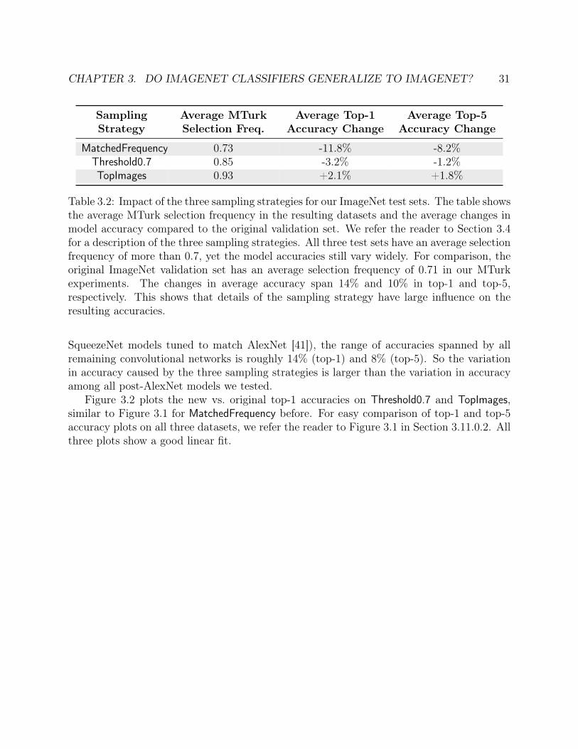
CHAPTER 3. DO IMAGENET CLASSIFIERS GENERALIZE TO IMAGENET? 31
SamplingStrategy
Average MTurkSelection Freq.
Average Top-1Accuracy Change
Average Top-5Accuracy Change
MatchedFrequency 0.73 -11.8% -8.2%Threshold0.7 0.85 -3.2% -1.2%TopImages 0.93 +2.1% +1.8%
Table 3.2: Impact of the three sampling strategies for our ImageNet test sets. The table showsthe average MTurk selection frequency in the resulting datasets and the average changes inmodel accuracy compared to the original validation set. We refer the reader to Section 3.4for a description of the three sampling strategies. All three test sets have an average selectionfrequency of more than 0.7, yet the model accuracies still vary widely. For comparison, theoriginal ImageNet validation set has an average selection frequency of 0.71 in our MTurkexperiments. The changes in average accuracy span 14% and 10% in top-1 and top-5,respectively. This shows that details of the sampling strategy have large influence on theresulting accuracies.
SqueezeNet models tuned to match AlexNet [41]), the range of accuracies spanned by allremaining convolutional networks is roughly 14% (top-1) and 8% (top-5). So the variationin accuracy caused by the three sampling strategies is larger than the variation in accuracyamong all post-AlexNet models we tested.
Figure 3.2 plots the new vs. original top-1 accuracies on Threshold0.7 and TopImages,similar to Figure 3.1 for MatchedFrequency before. For easy comparison of top-1 and top-5accuracy plots on all three datasets, we refer the reader to Figure 3.1 in Section 3.11.0.2. Allthree plots show a good linear fit.

CHAPTER 3. DO IMAGENET CLASSIFIERS GENERALIZE TO IMAGENET? 32
60 70 80Original test accuracy (top-1, %)
50
60
70
80
90
New
test
acc
urac
y (to
p-1,
%) ImageNet (New Test Set: Threshold.7)
60 70 80Original test accuracy (top-1, %)
50
60
70
80
90
New
test
acc
urac
y (to
p-1,
%) ImageNet (New Test Set: TopImages)
Ideal reproducibility Model accuracy Linear fitFigure 3.2: Model accuracy on the original ImageNet validation set vs. accuracy on twovariants of our new test set. We refer the reader to Section 3.4 for a description of these testsets. Each data point corresponds to one model in our testbed (shown with 95% Clopper-Pearson confidence intervals). On Threshold0.7, the model accuracies are 3% lower than onthe original test set. On TopImages, which contains the images most frequently selected byMTurk workers, the models perform 2% better than on the original test set. The accuracieson both datasets closely follow a linear function, similar to MatchedFrequency in Figure 3.1.The red shaded region is a 95% confidence region for the linear fit from 100,000 bootstrapsamples.

CHAPTER 3. DO IMAGENET CLASSIFIERS GENERALIZE TO IMAGENET? 33
3.5 CIFAR-10 experiment detailsWe first present our reproducibility experiment for the CIFAR-10 image classification dataset[53]. There are multiple reasons why CIFAR-10 is an important example for measuring howwell current models generalize to unseen data.
• CIFAR-10 is one of the most widely used datasets in machine learning and serves as atest ground for many image classification methods. A concrete measure of popularityis the fact that CIFAR-10 was the second most common dataset in NIPS 2017 (afterMNIST) [30].
• The dataset creation process for CIFAR-10 is transparent and well documented [53].Importantly, CIFAR-10 draws from the larger Tiny Images repository that has morefine-grained labels than the ten CIFAR-10 classes [93]. This enables us to minimizevarious forms of distribution shift between the original and new test set.
• CIFAR-10 poses a difficult enough problem so that the dataset is still the subject ofactive research (e.g., see [16, 28, 98, 104, 76, 13]). Moreover, there is a wide rangeof classification models that achieve significantly different accuracy scores. Since codefor these models has been published in various open source repositories, they can betreated as independent of our new test set.
Compared to ImageNet, CIFAR-10 is significantly smaller both in the number of imagesand in the size of each image. This makes it easier to conduct various follow-up experimentsthat require training new classification models. Moreover, the smaller size of CIFAR-10 alsomeans that the dataset has been accessible to more researchers for a longer time. Hence itis plausible that CIFAR-10 experienced more test set adaptivity than ImageNet, where it ismuch more costly to tune hyperparameters.
Before we describe how we created our new test set, we briefly review relevant backgroundon CIFAR-10 and Tiny Images.
Tiny Images. The dataset contains 80 million RGB color images with resolution 32 × 32pixels and was released in 2007 [93]. The images are organized by roughly 75,000 keywordsthat correspond to the non-abstract nouns from the WordNet database [65] Each keywordwas entered into multiple Internet search engines to collect roughly 1,000 to 2,500 imagesper keyword. It is important to note that Tiny Images is a fairly noisy dataset. Many ofthe images filed under a certain keyword do not clearly (or not at all) correspond to therespective keyword.
CIFAR-10. The CIFAR-10 dataset was created as a cleanly labeled subset of Tiny Imagesfor experiments with multi-layer networks. To this end, the researchers assembled a datasetconsisting of ten classes with 6,000 images per class, which was published in 2009 [53]. Theseclasses are airplane, automobile, bird, cat, deer, dog, frog, horse, ship, and truck.

CHAPTER 3. DO IMAGENET CLASSIFIERS GENERALIZE TO IMAGENET? 34
The standard train / test split is class-balanced and contains 50,000 training images and10,000 test images.
The CIFAR-10 creation process is well-documented [53]. First, the researchers assembleda set of relevant keywords for each class by using the hyponym relations in WordNet [65](for instance, “Chihuahua” is a hyponym of “dog”). Since directly using the correspondingimages from Tiny Images would not give a high quality dataset, the researchers paid studentannotators to label the images from Tiny Images. The labeler instructions can be found inSection C of [53] and include a set of specific guidelines (e.g., an image should not containtwo object of the corresponding class). The researchers then verified the labels of the imagesselected by the annotators and removed near-duplicates from the dataset via an `2 nearestneighbor search.
3.5.1 Dataset creation methodology
Our overall goal was to create a new test set that is as close as possible to being drawn fromthe same distribution as the original CIFAR-10 dataset. One crucial aspect here is that theCIFAR-10 dataset did not exhaust any of the Tiny Image keywords it is drawn from. So bycollecting new images from the same keywords as CIFAR-10, our new test set can match thesub-class distribution of the original dataset.
Understanding the Sub-Class Distribution. As the first step, we determined the TinyImage keyword for every image in the CIFAR-10 dataset. A simple nearest-neighbor searchsufficed since every image in CIFAR-10 had an exact duplicate (`2-distance 0) in Tiny Images.Based on this information, we then assembled a list of the 25 most common keywords foreach class. We decided on 25 keywords per class since the 250 total keywords make upmore than 95% of CIFAR-10. Moreover, we wanted to avoid accidentally creating a harderdataset with infrequent keywords that the classifiers had little incentive to learn based onthe original CIFAR-10 dataset.
The keyword distribution can be found in Section 3.10.0.1. Inspecting this list reveals theimportance of matching the sub-class distribution. For instance, the most common keywordin the airplane class is stealth_bomber and not a more common civilian type of airplane.In addition, the third most common keyword for the airplane class is stealth_fighter.Both types of planes are highly distinctive. There are more examples where certain sub-classes are considerably different. For instance, trucks from the keyword fire_truck aremostly red, which is quite different from pictures for dump_truck or other keywords.
Collecting new images. After determining the keywords, we collected correspondingimages. To simulate the student / researcher split in the original CIFAR-10 collection proce-dure, we introduced a similar split among two authors of this paper. Author A took the roleof the original student annotators and selected new suitable images for the 250 keywords.In order to ensure a close match between the original and new images for each keyword, we

CHAPTER 3. DO IMAGENET CLASSIFIERS GENERALIZE TO IMAGENET? 35
built a user interface that allowed Author A to first look through existing CIFAR-10 imagesfor a given keyword and then select new candidates from the remaining pictures in TinyImages. Author A followed the labeling guidelines in the original instruction sheet [53]. Thenumber of images Author A selected per keyword was so that our final dataset would containbetween 2,000 and 4,000 images. We decided on 2,000 images as a target number for tworeasons:
• While the original CIFAR-10 test set contains 10,000 images, a test set of size 2,000is already sufficient for a fairly small confidence interval. In particular, a conservativeconfidence interval (Clopper-Pearson at confidence level 95%) for accuracy 90% hassize about ±1% with n = 2,000 (to be precise, [88.6%, 91.3%]). Since we considereda potential discrepancy between original and new test accuracy only interesting if itis significantly larger than 1%, we decided that a new test set of size 2,000 was largeenough for our study.
• As with very infrequent keywords, our goal was to avoid accidentally creating a hardertest set. Since some of the Tiny Image keywords have only a limited supply of remainingadequate images, we decided that a smaller target size for the new dataset would reducebias to include images of more questionable difficulty.
After Author A had selected a set of about 9,000 candidate images, Author B adopted the roleof the researchers in the original CIFAR-10 dataset creation process. In particular, Author Breviewed all candidate images and removed images that were unclear to Author B or did notconform to the labeling instructions in their opinion (some of the criteria are subjective). Inthe process, a small number of keywords did not have enough images remaining to reach then = 2,000 threshold. Author B then notified Author A about the respective keywords andAuthor A selected a further set of images for these keywords. In this process, there was onlyone keyword where Author A had to carefully examine all available images in Tiny Images.This keyword was alley_cat and comprises less than 0.3% of the overall CIFAR-10 dataset.
Final assembly. After collecting a sufficient number of high-quality images for each key-word, we sampled a random subset from our pruned candidate set. The sampling procedurewas such that the keyword-level distribution of our new dataset matches the keyword-leveldistribution of CIFAR-10 (see Section 3.10.0.1). In the final stage, we again proceeded simi-lar to the original CIFAR-10 dataset creation process and used `2-nearest neighbors to filterout near duplicates. In particular, we removed near-duplicates within our new dataset andalso images that had a near duplicate in the original CIFAR-10 dataset (train or test). Thelatter aspect is particularly important since our reproducibility study is only interesting if weevaluate on truly unseen data. Hence we manually reviewed the top-10 nearest neighbors foreach image in our new test set. After removing near-duplicates in our dataset, we re-sampledthe respective keywords until this process converged to our final dataset.
Figure 3.3b shows a random subset of images from the original and our new test set.

CHAPTER 3. DO IMAGENET CLASSIFIERS GENERALIZE TO IMAGENET? 36
(a) Test set A (b) Test set B
Figure 3.3: Randomly selected images from the original and new CIFAR-10 test sets. Eachgrid contains two images for each of the ten classes. The following footnote reveals which ofthe two grids corresponds to the new test set.7
We remark that we did not run any classifiers on our new dataset during the data col-lection phase of our study. In order to ensure that the new data does not depend on theexisting classifiers, it is important to strictly separate the data collection phase from thefollowing evaluation phase.
3.5.2 Follow-up hypotheses
Since the gap between original and new accuracy is concerningly large, we investigatedmultiple hypotheses for explaining this gap.
3.5.2.1 Statistical Error
A first natural guess is that the gap is simply due to statistical fluctuations. But as notedbefore, the sample size of our new test set is large enough so that a 95% confidence interval hassize about ±1.2%. Since a 95% confidence interval for the original CIFAR-10 test accuracy iseven smaller (roughly ±0.6% for 90% classification accuracy and ±0.3% for 97% classificationaccuracy), we can rule out statistical error as the main explanation.
3.5.2.2 Differences in Near-Duplicate Removal
As mentioned in Section 3.5.1, the final step of both the original CIFAR-10 and our datasetcreation procedure is to remove near-duplicates. While removing near-duplicates betweenour new test set and the original CIFAR-10 dataset, we noticed that the original test setcontained images that we would have ruled out as near-duplicates. A large number ofnear-duplicates between CIFAR-10 train and test, combined with our more stringent near-duplicate removal, could explain some of the accuracy drop. Indeed, we found about 800

CHAPTER 3. DO IMAGENET CLASSIFIERS GENERALIZE TO IMAGENET? 37
images in the original CIFAR-10 test set that we would classify as near-duplicates (8% ofthe entire test set). Moreover, most classifiers have accuracy between 99% and 100% onthese near-duplicates (recall that most models achieve 100% training error). However, thefollowing calculation shows that the near-duplicates can explain at most 1% of the observeddifference.
For concreteness, we consider a model with 93% original test set accuracy such as acommon VGG or ResNet architecture. Let acctrue be the “true” accuracy of the model ontest images that are not near-duplicates, and let accnd be the accuracy on near-duplicates.Then for 8% near-duplicates, the overall accuracy is given by
acc = 0.92 · acctrue + 0.08 · accnd .
Using acc = 0.93, accnd = 1.0, and solving for acctrue then yields acctrue ≈ 0.924. So theaccuracy on original test images that are not near-duplicates is indeed lower, but only bya small amount (0.6%). This is in contrast to the 8% - 9% accuracy drop that VGG andResNet models with 93% original accuracy see in our experiments.
For completeness, we describe our process for finding near duplicates in detail. For everytest image, we visually inspected the top-10 nearest neighbors in both `2-distance and theSSIM (structural similarity) metric. We compared the original test set to the CIFAR-10training set, and our new test set to both the original training and test sets. We consideran image pair as near-duplicates if both images have the same object in the same pose. Weinclude images that have different zoom, color scale, stretch in the horizontal or verticaldirection, or small shifts in vertical or horizontal position. If the object was rotated or in adifferent pose, we did not include it as a near-duplicate.
3.5.2.3 Hyperparameter Tuning
Another conjecture is that we can recover some of the missing accuracy by re-tuning hyper-parameters of a model. To this end, we performed a grid search over multiple parametersof a VGG model. We selected three standard hyperparameters known to strongly influencetest set performance: initial learning rate, dropout, and weight decay. The vgg16_kerasarchitecture uses different amounts of dropout across different layers of the network, so wechose to tune a multiplicative scaling factor for the amount of dropout. This keeps the ratioof dropout across different layers constant.
We initialized a hyperparameter configuration from values tuned to the original test set(learning rate 0.1, dropout ratio 1, weight decay 5×10⁻⁴), and performed a grid search acrossthe following values:
• Learning rate in {0.0125, 0.025, 0.05, 0.1, 0.2, 0.4, 0.8}.
• Dropout ratio in {0.5, 0.75, 1, 1.25, 1.75}.7Test Set A is the new test set and Test Set B is the original test set.

CHAPTER 3. DO IMAGENET CLASSIFIERS GENERALIZE TO IMAGENET? 38
• Weight decay in {5×10⁻⁵, 1×10⁻⁴, 5×10⁻⁴, 1×10⁻³, 5×10⁻³}.
We ensured that the best performance was never at an extreme point of any range wetested for an individual hyperparameter. Overall, we did not find a hyperparameter settingwith a significantly better accuracy on the new test set (the biggest improvement was from85.3% to 85.8%).
3.5.2.4 Visually Inspecting Hard Images
It is also possible that we accidentally created a more difficult test set by including a setof “harder” images. To explore this question, we visually inspected the set of images thatmost models incorrectly classified. Figure 3.11 in Section 3.10.0.5 shows examples of thehard images in our new test set that no model correctly classified. We find that all the newimages are valid images that are recognizable to humans.
3.5.2.5 Human Accuracy Comparison
The visual inspection of hard images in the previous section is one way to compare theoriginal and new test sets. However, our conclusion may be biased since we have created thenew test set ourselves. To compare the relative hardness of the two test sets more objectively,we also conducted a small experiment to measure human accuracy on the two test sets.8 Thegoal of the experiment was to measure if human accuracy is significantly different on theoriginal and new test sets.
Since we conjectured that our new test set included particularly hard images, we focusedour experiment on the approximately 5% hardest images in both test sets. Here, “hardness”is defined by how many models correctly classified an image. After rounding to include allimages that were classified by the same number of models, we obtained 500 images from theoriginal test set and 115 images from our new test set.
We recruited nine graduate students from three different research groups in the ElectricalEngineering & Computer Sciences Department at UC Berkeley. We wrote a simple userinterface that allowed the participants to label images with one of the ten CIFAR-10 classes.To ensure that the participants did not know which dataset an image came from, we presentedthe images in random order.
Table 3.3 shows the results of our experiment. We find that four participants performedbetter on the original test set and five participants were better on our new test set. Theaverage difference is -0.8%, i.e., the participants do not see a drop in average accuracy onthis subset of original and new test images. This suggests that our new test set is notsignificantly harder for humans. However, we remark that our results here should only beseen as a preliminary study. Understanding human accuracy on CIFAR-10 in more detailwill require further experiments.
8Use of this data was permitted by the Berkeley Committee for Protection of Human Subjects (CPHS).

CHAPTER 3. DO IMAGENET CLASSIFIERS GENERALIZE TO IMAGENET? 39
Human Accuracy (%)
Original Test Set New Test Set Gap
Participant 1 85 [81.6, 88.0] 83 [74.2, 89.8] 2Participant 2 83 [79.4, 86.2] 81 [71.9, 88.2] 2Participant 3 82 [78.3, 85.3] 78 [68.6, 85.7] 4Participant 4 79 [75.2, 82.5] 84 [75.3, 90.6] -5Participant 5 76 [72.0, 79.7] 77 [67.5, 84.8] -1Participant 6 75 [71.0, 78.7] 73 [63.2, 81.4] 2Participant 7 74 [69.9, 77.8] 79 [69.7, 86.5] -5Participant 8 74 [69.9, 77.8] 76 [66.4, 84.0] -2Participant 9 67 [62.7, 71.1] 71 [61.1, 79.6] -4
Table 3.3: Human accuracy on the “hardest” images in the original and our new CIFAR-10test set. We ordered the images by number of incorrect classifications from models in ourtestbed and then selected the top 5% images from the original and new test set (500 imagesfrom the original test set, 115 images from our new test set). The results show that onaverage humans do not see a drop in accuracy on this subset of images.
3.5.2.6 Training on Part of Our New Test Set
If our new test set distribution is significantly different from the original CIFAR-10 distri-bution, retraining on part of our new test set (plus the original training data) may improvethe accuracy on the held-out fraction of our new test set.
We conducted this experiment by randomly drawing a class-balanced split containingabout 1,000 images from the new test set. We then added these images to the full CIFAR-10training set and retrained the vgg16_kerasmodel. After training, we tested the model on theremaining half of the new test set. We repeated this experiment twice with different randomlyselected splits from our test set, obtaining accuracies of 85.1% and 85.4% (compared to 84.9%without the extra training data9). This provides evidence that there is no large distributionshift between our new test set and the original CIFAR-10 dataset, or that the model is unableto learn the modified distribution.
3.5.2.7 Cross-validation
Cross-validation can be a more reliable way of measuring a model’s generalization abilitythan using only a single train / test split. Hence we tested if cross-validation on the originalCIFAR-10 dataset could predict a model’s error on our new test set. We created cross-validation data by randomly dividing the training set into 5 class-balanced splits. We then
9This number is slightly lower than the accuracy of vgg16_keras on our new test set in Table 3.12, butstill within the 95% confidence interval [83.6, 86.8]. Hence we conjecture that the difference is due to therandom fluctuation arising from randomly initializing the model.

CHAPTER 3. DO IMAGENET CLASSIFIERS GENERALIZE TO IMAGENET? 40
randomly shuffled together 4 out of the 5 training splits with the original test set. Theleftover held-out split from the training set then became the new test set.
We retrained the models vgg_15_BN_64, wide_resnet_28_10, and shake_shake_64d_cutouton each of the 5 new datasets we created. The accuracies are reported in Table 3.4. Theaccuracies on the cross-validation splits did not differ much from the accuracy on the originaltest set. The variation among the cross-validation splits is significantly smaller than the dropon our new test set.
Model Accuracy (%)
Dataset vgg_15_BN_64 wide_resnet_28_10 shake_shake_64d_cutout
Original Test Set 93.6 [93.1, 94.1] 95.7 [95.3, 96.1] 97.1 [96.8, 97.4]
Split 1 93.9 [93.4, 94.3] 96.2 [95.8, 96.6] 97.2 [96.9, 97.5]Split 2 93.8 [93.3, 94.3] 96.0 [95.6, 96.4] 97.3 [97.0, 97.6]Split 3 94.0 [93.5, 94.5] 96.4 [96.0, 96.8] 97.4 [97.1, 97.7]Split 4 94.0 [93.5, 94.5] 96.2 [95.8, 96.6] 97.4 [97.1, 97.7]Split 5 93.5 [93.0, 94.0] 96.5 [96.1, 96.9] 97.4 [97.1, 97.7]
New Test Set 84.9 [83.2, 86.4] 89.7 [88.3, 91.0] 93.0 [91.8, 94.1]
Table 3.4: Model accuracies on cross-validation splits for the original CIFAR-10 data. Thedifference in cross-validation accuracies is significantly smaller than the drop to the new testset.
3.5.2.8 Training a Discriminator for Original vs. New Test Set
Our main hypothesis for the accuracy drop is that small variations in the test set creationprocess suffice to significantly reduce a model’s accuracy. To test whether these variationscould be detected by a convolutional network, we investigated whether a discriminator modelcould distinguish between the two test sets.
We first created a training set consisting of 3, 200 images (1,600 from the original testset and 1,600 from our new test set) and a test set of 800 images (consisting of 400 imagesfrom original and new test set each). Each image had a binary label indicating whether itcame from the original or new test set. Additionally, we ensured that that both datasetswere class balanced.
We then trained resnet_32 and resnet_110 models for 160 epochs using a standardSGD optimizer to learn a binary classifier between the two datasets. We conducted twovariants of this experiment: in one variant, we trained the model from scratch. In the othervariant, we started with a model pre-trained on the regular CIFAR-10 classification task.
Our results are summarized in Table 3.5. Overall we found that the resulting modelscould not discriminate well between the original and our new test set: the best accuracy weobtained is 53.1%.

CHAPTER 3. DO IMAGENET CLASSIFIERS GENERALIZE TO IMAGENET? 41
Model Discriminator Accuracy (%) Discriminator Accuracy (%)random initialization pre-trained
resnet_32 50.1 [46.6, 53.6] 52.9 [49.4, 56.4]resnet_110 50.3 [46.7, 53.8] 53.1 [49.6, 56.6]
Table 3.5: Accuracies for discriminator models trained to distinguish between the originaland new CIFAR-10 test sets. The models were initialized either randomly or using a modelpre-trained on the original CIFAR-10 dataset. Although the models performed slightly betterthan random chance, the confidence intervals (95% Clopper Pearson) still overlap with 50%accuracy.
3.5.2.9 An Exactly Class-balanced Test Set
The top 25 keywords of each class in CIFAR-10 capture approximately 95% of the dataset.However, the remaining 5% of the dataset are skewed towards the class ship. As a result,our new dataset was not exactly class-balanced and contained only 8% images of class ship(as opposed to 10% in the original test set).
To measure whether this imbalance affected the accuracy scores, we created an exactlyclass-balanced version of our new test set with 2,000 images (200 per class). In this version,we selected the top 50 keywords in each class and computed a fractional number of imagesfor each keyword. We then rounded these numbers so that images for keywords with thelargest fractional part were added first. The resulting model accuracies can be found inTable 3.13 (Section 3.10.0.4). Models with lower original accuracies achieve a small accuracyimprovement on the exactly class-balanced test set (around 0.3%), but the accuracy drop ofthe best-performing model remains unchanged.

CHAPTER 3. DO IMAGENET CLASSIFIERS GENERALIZE TO IMAGENET? 42
3.6 ImageNet experiment detailsOur results on CIFAR-10 show that current models fail to reliably generalize in the presenceof small variations in the data distribution. One hypothesis is that the accuracy drop stemsfrom the limited nature of the CIFAR-10 dataset. Compared to other datasets, CIFAR-10 isrelatively small, both in terms of image resolution and the number of images in the dataset.Since the CIFAR-10 models are only exposed to a constrained visual environment, they maybe unable to learn a more reliable representation.
To investigate whether ImageNet models generalize more reliably, we assemble a newtest set for ImageNet. ImageNet captures a much broader variety of natural images: itcontains about 24× more training images than CIFAR-10 with roughly 100× more pixelsper image. As a result, ImageNet poses a significantly harder problem and is among themost prestigious machine learning benchmarks. The steadily improving accuracy numbershave also been cited as an important breakthrough in machine learning [62]. If popularImageNet models are indeed more robust to natural variations in the data (and there isagain no adaptive overfitting), the accuracies on our new test set should roughly match theexisting accuracies.
Before we proceed to our experiments, we briefly describe the relevant background con-cerning the ImageNet dataset. For more details, we refer the reader to the original ImageNetpublications [15, 81].
ImageNet. ImageNet [15, 81] is a large image database consisting of more than 14 millionhuman-annotated images depicting almost 22,000 classes. The images do not have a uniformsize, but most of them are stored as RGB color images with a resolution around 500 × 400pixels. The classes are derived from the WordNet hierarchy [65], which represents each classby a set of synonyms (“synset”) and is organized into semantically meaningful relations. Eachclass has an associated definition (“gloss”) and a unique WordNet ID (“wnid”).
The ImageNet team populated the classes with images downloaded from various imagesearch engines, using the WordNet synonyms as queries. The researchers then annotated theimages via Amazon Mechanical Turk (MTurk). A class-specific threshold decided how manyagreements among the MTurk workers were necessary for an image to be considered valid.Overall, the researchers employed over 49,000 workers from 167 countries [55].
Since 2010, the ImageNet team has run the yearly ImageNet Large Scale Visual Recog-nition Challenge (ILSVRC), which consists of separate tracks for object classification, local-ization, and detection. All three tracks are based on subsets of the ImageNet data. Theclassification track has received the most attention and is also the focus of this chapter.
The ILSVRC2012 competition data has become the de facto benchmark version of thedataset and comprises 1.2 million training images, 50,000 validation images, and 100,000 testimages depicting 1,000 categories. We generally refer to this data as the ImageNet training,validation, and test set. The labels for the ImageNet test set were never publicly releasedin order to minimize adaptive overfitting. Instead, teams could submit a limited number ofrequests to an evaluation server in order to obtain accuracy scores. There were no similar

CHAPTER 3. DO IMAGENET CLASSIFIERS GENERALIZE TO IMAGENET? 43
limitations in place for the validation set. Most publications report accuracy numbers onthe validation set.
The training, validation, and test sets were not drawn strictly i.i.d. from the same dis-tribution (i.e., there was not a single data collection run with the result split randomly intotraining, validation, and test). Instead, the data collection was an ongoing process and boththe validation and test sets were refreshed in various years of the ILSVRC. One notable dif-ference is that the ImageNet training and validation sets do not have the same data source:while the ImageNet training set consists of images from several search engines (e.g., Google,MSN, Yahoo, and Flickr), the validation set consists almost entirely of images from Flickr[1].
3.6.1 Dataset creation methodology
Since the existing training, validation, and test sets are not strictly i.i.d. (see above), thefirst question was which dataset part to replicate. For our experiment, we decided to matchthe distribution of the validation set. There are multiple reasons for this choice:
• In contrast to the training set, the validation set comes from only one data source(Flickr). Moreover, the Flickr API allows fine-grained searches, which makes it easierto control the data source and match the original distribution.
• In contrast to the original test set, the validation set comes with label information.This makes it easier to inspect the existing image distribution for each class, which isimportant to ensure that we match various intricacies of the dataset (e.g., see Section3.11.0.6 for examples of ambiguous classes).
• Most papers report accuracy numbers on the validation set. Hence comparing new vs.existing accuracies is most relevant for the validation set.
• The validation set is commonly used to develop new architectures and tune hyperpa-rameters, which leads to the possibility of adaptive overfitting. If we again observeno diminishing returns in accuracy on our new test set, this indicates that even thevalidation set is resilient to adaptive overfitting.
Therefore, our goal was to replicate the distribution of the original validation set asclosely as possible. We aimed for a new test set of size 10,000 since this would already resultin accuracy scores with small confidence intervals (see Section 3.2). While a larger datasetwould result in even smaller confidence intervals, we were also concerned that searching formore images might lead to a larger distribution shift. In particular, we decided to use a timerange for our Flickr queries after the original ImageNet collection period (see below for thecorresponding considerations). Since a given time period only has a limited supply of highquality images, a larger test set would have required a longer time range. This in turn maycreate a larger temporal distribution shift. To balance these two concerns, we decided on asize of 10,000 images for the new test set.
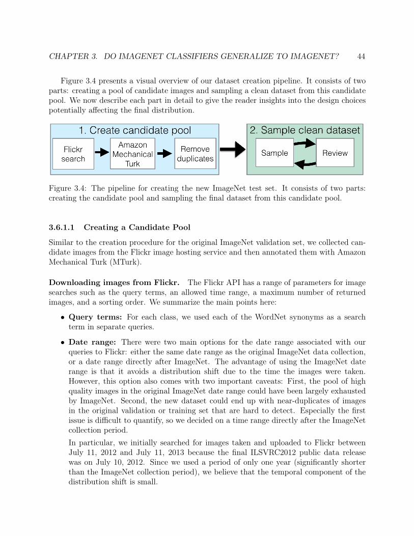
CHAPTER 3. DO IMAGENET CLASSIFIERS GENERALIZE TO IMAGENET? 44
Figure 3.4 presents a visual overview of our dataset creation pipeline. It consists of twoparts: creating a pool of candidate images and sampling a clean dataset from this candidatepool. We now describe each part in detail to give the reader insights into the design choicespotentially affecting the final distribution.
Figure 3.4: The pipeline for creating the new ImageNet test set. It consists of two parts:creating the candidate pool and sampling the final dataset from this candidate pool.
3.6.1.1 Creating a Candidate Pool
Similar to the creation procedure for the original ImageNet validation set, we collected can-didate images from the Flickr image hosting service and then annotated them with AmazonMechanical Turk (MTurk).
Downloading images from Flickr. The Flickr API has a range of parameters for imagesearches such as the query terms, an allowed time range, a maximum number of returnedimages, and a sorting order. We summarize the main points here:
• Query terms: For each class, we used each of the WordNet synonyms as a searchterm in separate queries.
• Date range: There were two main options for the date range associated with ourqueries to Flickr: either the same date range as the original ImageNet data collection,or a date range directly after ImageNet. The advantage of using the ImageNet daterange is that it avoids a distribution shift due to the time the images were taken.However, this option also comes with two important caveats: First, the pool of highquality images in the original ImageNet date range could have been largely exhaustedby ImageNet. Second, the new dataset could end up with near-duplicates of imagesin the original validation or training set that are hard to detect. Especially the firstissue is difficult to quantify, so we decided on a time range directly after the ImageNetcollection period.In particular, we initially searched for images taken and uploaded to Flickr betweenJuly 11, 2012 and July 11, 2013 because the final ILSVRC2012 public data releasewas on July 10, 2012. Since we used a period of only one year (significantly shorterthan the ImageNet collection period), we believe that the temporal component of thedistribution shift is small.

CHAPTER 3. DO IMAGENET CLASSIFIERS GENERALIZE TO IMAGENET? 45
• Result size: We initially downloaded up to 100 images for each class. If a class has ksynonyms associated with it, we requested 100/k images for each synonym. We decidedon 100 images per class since we aimed for 10,000 images overall and estimated that10% of the candidate images would be of sufficiently high quality (similar to ImageNet[15]).
• Result order: Flickr offers the sorting options “relevance”, “interestingness”, and vari-ous temporal orderings. Note that the “relevance” and “interestingness” orderings mayrely on machine learning models trained on ImageNet. Since these orderings may intro-duce a significant bias (e.g., by mainly showing images that current ImageNet modelsrecognize for the respective search term), we chose to order the images by their uploaddate. This helps to ensure that our new test set is independent of current classifiers.
After our first data collection, we found it necessary to expand the initial candidate poolfor particular classes in order to reach a sufficient number of valid images. This is similarto the original ImageNet creation process, where the authors expanded the set of queriesusing two methods [15, 81]. The first method appended a word from the parent class tothe queries if this word also appeared in the gloss of the target class. The second methodincluded translations of the queries into other languages such as Chinese, Spanish, Dutch,and Italian.
We took the following steps to expand our search queries, only proceeding to the nextstep for a given class when in need of more images.
1. Append a word from the parent class if the word appears in the gloss of the targetclass.
2. Expand the maximum number of images to 200 for this class.
3. Expand the search range to include photos taken or uploaded before July 11, 2014 (i.e.,a time span of two years instead of one).
4. Concatenate compound queries, i.e., search for “dialphone” instead of “dial phone”.
5. Manually pick alternative query words, including translations of the queries.
In total, we obtained 208,145 candidate images from Flickr.
Amazon Mechanical Turk. While the candidate images from Flickr are correlated withtheir corresponding class, a large number of images are still unsuitable for an image clas-sification dataset. For instance, the images may be of low quality (blurry, unclear objectpresence, etc.), violate dataset rules (e.g., no paintings), or be simply unrelated to the targetclass. So similar to ImageNet, we utilized MTurk to filter our pool of candidate images.
We designed our MTurk tasks and UI to be close to those used in ImageNet. As inImageNet, we showed each MTurk worker a grid of 48 candidate images for a given target

CHAPTER 3. DO IMAGENET CLASSIFIERS GENERALIZE TO IMAGENET? 46
class. The task description was derived from the original ImageNet instructions and includedthe definition of the target class with a link to a corresponding Wikipedia page. We askedthe MTurk workers to select images belonging to the target class regardless of “occlusions,other objects, and clutter or text in the scene” and to avoid drawings or paintings (both asin ImageNet). Section 3.6.1.2 shows a screenshot of our UI and a screenshot of the originalUI for comparison.
For quality control, we embedded at least six randomly selected images from the originalvalidation set in each MTurk task (three from the same class, three from a class that isnearby in the WordNet hierarchy). These images appeared in random locations of the imagegrid for each task. We obfuscated all image URLs and resized our images to match the mostcommon size of the existing validation images so that the original validation images werenot easy to spot.
The main outcome of the MTurk tasks is a selection frequency for each image, i.e., whatfraction of MTurk workers selected the image in a task for its target class. We recruitedat least ten MTurk workers for each task (and hence for each image), which is similar toImageNet. Since each task contained original validation images, we could also estimate howoften images from the original dataset were selected by our MTurk workers.
Removing near-duplicate images. The final step in creating the candidate pool wasto remove near-duplicates, both within our new test set and between our new test set andthe original ImageNet dataset. Both types of near-duplicates could harm the quality of ourdataset.
Since we obtained results from Flickr in a temporal ordering, certain events (e.g., the2012 Olympics) led to a large number of similar images depicting the same scene (e.g., in theclass for the “horizontal bar“ gymnastics instrument). Inspecting the ImageNet validation setrevealed only very few sets of images from a single event. Moreover, the ImageNet paper alsoremarks that they removed near-duplicates [15]. Hence we decided to remove near-duplicateswithin our new test set.
Near-duplicates between our dataset and the original test set are also problematic. Sincethe models typically achieve high accuracy on the training set, testing on a near-duplicateof a training image checks for memorization more than generalization. A near-duplicatebetween the existing validation set and our new test set also defeats the purpose of measuringgeneralization to previously unseen data (as opposed to data that may already have beenthe victim of adaptive overfitting).
To find near-duplicates, we computed the 30 nearest neighbors for each candidate imagein three different metrics: `2-distance on raw pixels, `2-distance on features extracted from apre-trained VGG [84] model (fc7), and SSIM (structural similarity) [94], which is a popularimage similarity metric. For metrics that were cheap to evaluate (`2-distance on pixels and`2-distance on fc7), we computed nearest neighbor distances to all candidate images and allof the original ImageNet data. For the more compute-intensive SSIM metric, we restrictedthe set of reference images to include all candidate images and the five closest ImageNet

CHAPTER 3. DO IMAGENET CLASSIFIERS GENERALIZE TO IMAGENET? 47
classes based on the tree distance in the WordNet hierarchy. We then manually reviewednearest neighbor pairs below certain thresholds for each metric and removed any duplicateswe discovered.
To the best of our knowledge, ImageNet used only nearest neighbors in the `2-distanceto find near-duplicates [1]. While this difference may lead to a small change in distribution,we still decided to use multiple metrics since including images that have near-duplicatesin ImageNet would be contrary to the main goal of our experiment. Moreover, a manualinspection of the original validation set revealed only a very small number of near-duplicateswithin the existing dataset.
3.6.1.2 MTurk user interfaces
For comparison, we include the original ImageNet MTurk user interface (UI) in Figure 3.5and the MTurk UI we used in our experiments in Figure 3.6. Each UI corresponds to onetask for the MTurk workers, which consists of 48 images in both cases. In contrast to theoriginal ImageNet UI, our UI takes up more than one screen. This requires the MTurkworkers to scroll but also provides more details in the images. While the task descriptionsare not exactly the same, they are very similar and contain the same directions (e.g., bothdescriptions ask the MTurk workers to exclude drawings or paintings).
Figure 3.5: The user interface employed in the original ImageNet collection process for thelabeling tasks on Amazon Mechanical Turk.

CHAPTER 3. DO IMAGENET CLASSIFIERS GENERALIZE TO IMAGENET? 48
Figure 3.6: Our user interface for labeling tasks on Amazon Mechanical Turk. The screenshothere omits the scroll bar and shows only a subset of the entire MTurk task. As in theImageNet UI, the full task involves a grid of 48 images.

CHAPTER 3. DO IMAGENET CLASSIFIERS GENERALIZE TO IMAGENET? 49
3.6.1.3 User interface for our final reviewing process
Figure 3.7 shows a screenshot of the reviewing UI that we used to manually review the newImageNet datasets. At the top, the UI displays the wnid (“n01667114”), the synset (mudturtle), and the gloss. Next, a grid of 20 images is shown in 4 rows.
The top two rows correspond to the candidate images currently sampled for the newdataset. Below each image, our UI shows a unique identifier for the image and the date theimage was taken. There is also a check box to blacklist any incorrect images. In addition,there is a check box for each image to add it to the blacklist of incorrect images. If animage is added to the blacklist, it will be removed in the next revision of the dataset andreplaced with a new image from the candidate pools. The candidate images are sorted bythe date they were taken, which makes it easier to spot and remove near-duplicates. Imagesare marked as near-duplicates by adding their identifier to the “Near-duplicate set” text field.
The bottom two rows correspond to a random sample of images from the validation setthat belong to the target class. We display these images to make it easier to detect andcorrect for distribution shifts between our new test sets and the original ImageNet validationdataset.
3.6.1.4 Sampling a Clean Dataset
The result of collecting a candidate pool was a set of images with annotations from MTurk,most importantly the selection frequency of each image. In the next step, we used thiscandidate pool to sample a new test set that closely resembles the distribution of the existingvalidation set. There were two main difficulties in this process.
First, the ImageNet publications do not provide the agreement thresholds for each classthat were used to determine which images were valid. One possibility could be to run thealgorithm the ImageNet authors designed to compute the agreement thresholds. However,this algorithm would need to be exactly specified, which is unfortunately not the case to thebest of our knowledge.10
Second, and more fundamentally, it is impossible to exactly replicate the MTurk workerpopulation from 2010 – 2012 with a reproducibility experiment in 2018. Even if we hadaccess to the original agreement thresholds, it is unclear if they would be meaningful for ourMTurk data collection (e.g., because the judgments of our annotations could be different).Similarly, re-running the algorithm for computing agreement thresholds could give differentresults with our MTurk worker population.
10To be precise: Jia Deng’s PhD thesis [14] provides a clear high-level description of their algorithmfor computing agreement thresholds. However – as is commonly the case in synopses of algorithms – thedescription still omits some details such as the binning procedure or the number of images used to computethe thresholds. Since it is usually hard to exactly reconstruct a non-trivial algorithm from an informalsummary, we instead decided to implement three different sampling strategies and compare their outcomes.Potential deviations from the ImageNet sampling procedure are also alleviated by the fact that our MTurktasks always included at least a few images from the original validation set, which allowed us to calibrateour sampling strategies to match the existing ImageNet data.

CHAPTER 3. DO IMAGENET CLASSIFIERS GENERALIZE TO IMAGENET? 50
So instead of attempting to directly replicate the original agreement thresholds, we in-stead explored three different sampling strategies. An important asset in this part of ourexperiment was that we had inserted original validation images into the MTurk tasks (seethe previous subsection). So at least for our MTurk worker population, we could estimatehow frequently the MTurk workers select the original validation images.
In this subsection, we describe our sampling strategy that closely matches the selectionfrequency distribution of the original validation set. The follow-up experiments in Section3.4 then explore the impact of this design choice in more detail. As we will see, the samplingstrategy has significant influence on the model accuracies.
Matching the Per-class Selection Frequency. A simple approach to matching theselection frequency of the existing validation set would be to sample new images so that themean selection frequency is the same as for the original dataset. However, a closer inspectionof the selection frequencies reveals significant differences between the various classes. Forinstance, well-defined and well-known classes such as “African elephant” tend to have highselection frequencies ranging from 0.8 to 1.0. At the other end of the spectrum are classeswith an unclear definition or easily confused alternative classes. For instance, the MTurkworkers in our experiment often confused the class “nail” (the fastener) with fingernails, whichled to significantly lower selection frequencies for the original validation images belonging tothis class. In order to match these class-level details, we designed a sampling process thatapproximately matches the selection frequency distribution for each class.
As a first step, we built an estimate of the per-class distribution of selection frequencies.For each class, we divided the annotated validation images into five histogram bins based ontheir selection frequency. These frequency bins were [0.0, 0.2), [0.2, 0.4), [0.4, 0.6), [0.6, 0.8),and [0.8, 1.0]. Intuitively, these bins correspond to a notion of image quality assessed bythe MTurk workers, with the [0.0, 0.2) bin containing the worst images and the [0.8, 1.0] bincontaining the best images. Normalizing the resulting histograms then yielded a distributionover these selection frequency bins for each class.
Next, we sampled ten images for each class from our candidate pool, following the dis-tribution given by the class-specific selection frequency histograms. More precisely, we firstcomputed the target number of images for each histogram bin, and then sampled from thecandidates images falling into this histogram bin uniformly at random. Since we only had alimited number of images for each class, this process ran out of images for a small numberof classes. In these cases, we then sampled candidate images from the next higher bin untilwe found a histogram bin that still had images remaining. While this slightly changes thedistribution, we remark that it makes our new test set easier and only affected 0.8% of theimages in the new test set.
At the end of this sampling process, we had a test set with 10, 000 images and an averagesampling frequency of 0.73. This is close to the average sampling frequency of the annotatedvalidation images (0.71).

CHAPTER 3. DO IMAGENET CLASSIFIERS GENERALIZE TO IMAGENET? 51
Final Reviewing. While the methodology outlined so far closely matches the originalImageNet distribution, it is still hard to ensure that no unintended biases crept into thedataset (e.g., our MTurk workers could interpret some of the class definitions differentlyand select different images). So for quality control, we added a final reviewing step to ourdataset creation pipeline. Its purpose was to rule out obvious biases and ensure that thedataset satisfies our quality expectations before we ran any models on the new dataset. Thisminimizes dependencies between the new test set and the existing models.
In the final reviewing step, we manually reviewed every image in the dataset. Section3.6.1.3 includes a screenshot and brief description of the user interface. When we found anincorrect image or a near-duplicate, we removed it from the dataset. After a pass throughthe dataset, we then re-sampled new images from our candidate pool. In some cases, thisalso required new targeted Flickr searches for certain classes. We repeated this process untilthe dataset converged after 33 iterations. We remark that the majority of iterations onlychanged a small number of images.
One potential downside of the final reviewing step is that it may lead to a distributionshift. However, we accepted this possibility since we view dataset correctness to be moreimportant than minimizing distribution shift. In the end, a test set is only interesting ifit has correct labels. Note also that removing incorrect images from the dataset makes iteasier, which goes against the main trend we observe (a drop in accuracy). Finally, we kepttrack of all intermediate iterations of our dataset so that we could measure the impact ofthis final reviewing step (see Section 3.6.3.2). This analysis shows that the main trends (asignificant accuracy drop and an approximately linear relationship between original and newaccuracy) also hold for the first iteration of the dataset without any additional reviewing.
3.6.2 Model performance results
After assembling our new test sets, we evaluated a broad range of models on both the originalvalidation set and our new test sets. Section 3.11.0.1 contains a list of all models we evaluatedwith corresponding references and links to source code repositories. Tables 3.14 and 3.15show the top-1 and top-5 accuracies for our main test set MatchedFrequency. Figure 3.12visualizes the top-1 and top-5 accuracies on all three test sets.
In the main text of the chapter and Figure 3.12, we have chosen to exclude the FisherVector models and show accuracies only for the convolutional neural networks (convnets).Since the Fisher Vector models achieve significantly lower accuracy, a plot involving bothmodel families would have sacrificed resolution among the convnets. We decided to focus onconvnets in the main text because they have become the most widely used model family onImageNet.
Moreover, a linear model of accuracies (as shown in previous plots) is often not a goodfit when the accuracies span a wide range. Instead, a non-linear model such as a logisticor probit model can sometimes describe the data better. Indeed, this is also the case forour data on ImageNet. Figure 3.8 shows the accuracies both on a linear scale as in theprevious plots, and on a probit scale, i.e., after applying the inverse of the Gaussian CDF

CHAPTER 3. DO IMAGENET CLASSIFIERS GENERALIZE TO IMAGENET? 52
to all accuracy scores. As can be seen by comparing the two plots in Figure 3.8, the probitmodel is a better fit for our data. It accurately summarizes the relationship between originaland new test set accuracy for all models from both model families in our testbed.
Similar to Figure 3.12, we also show the top-1 and top-5 accuracies for all three datasetsin the probit domain in Figure 3.13. Section 3.7.3 describes a possible generative model thatleads to a linear fit in the probit domain as exhibited by the plots in Figures 3.8 and 3.13.
3.6.3 Follow-up hypotheses
As for CIFAR-10, the gap between original and new accuracy is concerningly large. Hencewe investigated multiple hypotheses for explaining this gap.
3.6.3.1 Cross validation
A natural question is whether cross-validation with the existing ImageNet data could havepointed towards a significant drop in accuracy. If adaptive overfitting to the images in thevalidation set is a cause for the accuracy drop, testing on different images from anothercross-validation fold could produce lower accuracies.11 Moreover, recall that the ImageNetvalidation set is not a strictly i.i.d. sample from the same distribution as the training set(see the beginning of Section 3.4). This also raises the question of how well a model wouldperform on a cross-validation fold from the training data.
To investigate these two effects, we conducted a cross-validation experiment with theImageNet training and validation sets. In order to ensure that the new cross-validationfolds contain only training images, we treated the existing validation set as one fold andcreated five additional folds with 50,000 images each. To this end, we drew a class-balancedsample of 250,000 images from the training set and then randomly partitioned this sampleinto five cross-validation folds (again class-balanced). For each of these five folds, we addedthe validation set (and the other training folds) to the training data so that the size of thetraining set was unchanged. We then trained one resnet50 model12 [32] for each of the fivetraining sets and evaluated them on the corresponding held-out data. Table 3.6 shows theresulting accuracies for each split.
Overall, we do not see a large difference in accuracy on the new cross validation splits:all differences fall within the 95% confidence intervals around the accuracy scores. This isin contrast to the significantly larger accuracy drops on our new test sets.
11Note however that the training images may also be affected by adaptive overfitting since the modelhyperparameters are often tuned for fast training speed and high training accuracy.
12To save computational resources, we used the optimized training code from https://github.com/fastai/imagenet-fast. Hence the top-5 accuracy on the original validation set is 0.4% lower than in Table3.15.

CHAPTER 3. DO IMAGENET CLASSIFIERS GENERALIZE TO IMAGENET? 53
Dataset resnet50 Top-5 Accuracy (%)
Original validation set 92.5 [92.3, 92.8]
Split 1 92.60 [92.4, 92.8]Split 2 92.59 [92.4, 92.8]Split 3 92.61 [92.4, 92.8]Split 4 92.55 [92.3, 92.8]Split 5 92.62 [92.4, 92.9]
New test set (MatchedFrequency) 84.7 [83.9, 85.4]
Table 3.6: resnet50 accuracy on cross-validation splits created from the original ImageNettrain and validation sets. The accuracy increase is likely caused by a small shift in distribu-tion between the ImageNet training and validation sets.
3.6.3.2 Impact of dataset revisions
As mentioned in Section 3.6.1.4, our final reviewing pass may have led to a distribution shiftcompared to the original ImageNet validation set. In general, our reviewing criterion was toblacklist images that were
• not representative of the target class,
• cartoons, paintings, drawings, or renderings,
• significantly different in distribution from the original ImageNet validation set,
• unclear, blurry, severely occluded, overly edited, or including only a small target object.
For each class, our reviewing UI (screenshot in Section 3.6.1.3) displayed a random sampleof ten original validation images directly next to the ten new candidate images currentlychosen. At least to some extent, this allowed us to detect and correct distribution shiftsbetween the original validation set and our candidate pool. As a concrete example, we notedin one revision of our dataset that approximately half of the images for “great white shark”were not live sharks in the water but models in museums or statues outside. In contrast,the ImageNet validation set had fewer examples of such artificial sharks. Hence we decidedto remove some non-live sharks from our candidate pool and sampled new shark images asa replacement in the dataset.
Unfortunately, some of these reviewing choices are subjective. However, such choicesare often an inherent part of creating a dataset and it is unclear whether a more “hands-off” approach would lead to more meaningful conclusions. For instance, if the drop inaccuracy was mainly caused by a distribution shift that is easy to identify and correct(e.g., an increase in black-and-white images), the resulting drop may not be an interestingphenomenon (beyond counting black-and-white images). Hence we decided to both remove

CHAPTER 3. DO IMAGENET CLASSIFIERS GENERALIZE TO IMAGENET? 54
distribution shifts that we found easy to identify visually, and also to measure the effect ofthese interventions.
Our reviewing process was iterative, i.e., we made a full pass over every incomplete classin a given dataset revision before sampling new images to fill the resulting gaps. Each timewe re-sampled our dataset, we saved the current list of images in our version control system.This allowed us to track the datasets over time and later measure the model accuracy foreach dataset revision. We remark that we only computed model accuracies on intermediaterevisions after we had arrived at the final revision of the corresponding dataset.
Figure 3.9 plots the top-1 accuracy of a resnet50 model versus the dataset revision forour new MatchedFrequency test set. Overall, reviewing improved model accuracy by about4% for this dataset. This is evidence that our manual reviewing did not cause the drop inaccuracy between the original and new dataset.
In addition, we also investigated whether the linear relationship between original andnew test accuracy was affected by our final reviewing passes. To this end, we evaluatedour model testbed on the first revision of our MatchedFrequency test set. As can be seen inFigure 3.10, the resulting accuracies still show a good linear fit that is of similar quality asin Figure 3.12. This shows that the linear relationship between the test accuracies is not aresult of our reviewing intervention.

CHAPTER 3. DO IMAGENET CLASSIFIERS GENERALIZE TO IMAGENET? 55
Figure 3.7: The user interface we built to review dataset revisions and remove incorrect ornear duplicate images. This user interface was not used for MTurk but only in the finaldataset review step conducted by the authors of this paper.

CHAPTER 3. DO IMAGENET CLASSIFIERS GENERALIZE TO IMAGENET? 56
20 30 40 50 60 70 80Original test accuracy (top-1, %)
10
20
30
40
50
60
70
80
New
test
acc
urac
y (to
p-1,
%) ImageNet (linear axis scaling)
20 30 40 50 60 70 80Original test accuracy (%)
10
20
3040506070
80
New
test
acc
urac
y (%
)
ImageNet (probit axis scaling)
Ideal reproducibility Model accuracy Linear fitFigure 3.8: Model accuracy on the original ImageNet validation set vs. our new test setMatchedFrequency. Each data point corresponds to one model in our testbed (shown with95% Clopper-Pearson confidence intervals), and we now also include the Fisher Vector mod-els. The left plot shows the model accuracies with a linear scale on the axes. The rightplot instead uses a probit scale, i.e., accuracy α appears at Φ−1(α), where Φ is the GaussianCDF. Comparing the two plot provides evidence that the probit model is a better fit for theaccuracy scores. Over a range of 60 percentage points, the linear fit in the probit domainaccurately describes the relationship between original and new test set accuracy. The shadedregion around the linear fit is a 95% confidence region from 100,000 bootstrap samples. Theconfidence region is present in both plots but is significantly smaller in the right plot due tothe better fit in the probit domain.

CHAPTER 3. DO IMAGENET CLASSIFIERS GENERALIZE TO IMAGENET? 57
1 3 5 7 9 11 13 15 17 19 21 23ImageNetV2-b version #
0.615
0.620
0.625
0.630
0.635
0.640
0.645
0.650
0.655
top
1 ac
cura
cy
version vs top 1 accuracy
1 3 5 7 9 11 13 15 17 19 21 23ImageNetV2-b version #
0.830
0.835
0.840
0.845
0.850
0.855
0.860
0.865
top
5 ac
cura
cy
version vs top 5 accuracy
2 4 6 8 10 12 14 16 18 20 22ImageNetV2-b version #
0
250
500
750
1000
1250
1500
1750
num
ber o
f im
ages
cha
nged
in v
ersio
n
Figure 3.9: Impact of the reviewing passes on the accuracy of a resnet152 on our newMatchedFrequency test set. The revision numbers correspond to the chronological orderingin which we created the dataset revisions

CHAPTER 3. DO IMAGENET CLASSIFIERS GENERALIZE TO IMAGENET? 58
60 70 80Original test accuracy (%)
40
50
60
70
80
90
New
test
acc
urac
y (%
)
ImageNet vs. MatchedFrequency, Top-1
80 90 100Original test accuracy (%)
60
70
80
90
100
New
test
acc
urac
y (%
)
ImageNet vs. MatchedFrequency, Top-5
Ideal reproducibility Model accuracy Linear fitFigure 3.10: Model accuracy on the original ImageNet validation set vs. accuracy on the firstrevision of our MatchedFrequency test set. Each data point corresponds to one model in ourtestbed (shown with 95% Clopper-Pearson confidence intervals). The red shaded region isa 95% confidence region for the linear fit from 100,000 bootstrap samples. The plots showthat the linear relationship between original and new test accuracy also occurs without ourfinal dataset reviewing step. The accuracy plots for the final revision of MatchedFrequencycan be found in Figure 3.12.

CHAPTER 3. DO IMAGENET CLASSIFIERS GENERALIZE TO IMAGENET? 59
3.7 DiscussionWe now return to the main question from Section 3.2: What causes the accuracy drops? Asbefore, we distinguish between two possible mechanisms.
3.7.1 Adaptivity gap
In its prototypical form, adaptive overfitting would manifest itself in diminishing returnsobserved on the new test set (see Section 3.2.1). However, we do not observe this pattern oneither CIFAR-10 or ImageNet. On both datasets, the slope of the linear fit is greater than1, i.e., each point of accuracy improvement on the original test set translates to more than1% on the new test set. This is the opposite of the standard overfitting scenario. So at leaston CIFAR-10 and ImageNet, multiple years of competitive test set adaptivity did not leadto diminishing accuracy numbers.
While our experiments rule out the most dangerous form of adaptive overfitting, weremark that they do not exclude all variants. For instance, it could be that any test setadaptivity leads to a roughly constant drop in accuracy. Then all models are affected equallyand we would see no diminishing returns since later models could still be better. Testing forthis form of adaptive overfitting likely requires a new test set that is truly i.i.d. and not theresult of a separate data collection effort. Finding a suitable dataset for such an experimentis an interesting direction for future research.
The lack of adaptive overfitting contradicts conventional wisdom in machine learning.We now describe two mechanisms that could have prevented adaptive overfitting:
The Ladder mechanism. Blum and Hardt introduced the Ladder algorithm to protectmachine learning competitions against adaptive overfitting [3]. The core idea is that con-strained interaction with the test set can allow a large number of model evaluations tosucceed, even if the models are chosen adaptively. Due to the natural form of their algo-rithm, the authors point out that it can also be seen as a mechanism that the machinelearning community implicitly follows.
Limited model class. Adaptivity is only a problem if we can choose among models forwhich the test set accuracy differs significantly from the population accuracy. Importantly,this argument does not rely on the number of all possible models (e.g., all parameter settingsof a neural network), but only on those models that could actually be evaluated on the testset. For instance, the standard deep learning workflow only produces models trained withSGD-style algorithms on a fixed training set, and requires that the models achieve hightraining accuracy (otherwise we would not consider the corresponding hyperparameters).Hence the number of different models arising from the current methodology may be smallenough so that uniform convergence holds.
Our experiments offer little evidence for favoring one explanation over the other. Oneobservation is that the convolutional networks shared many errors on CIFAR-10, which could

CHAPTER 3. DO IMAGENET CLASSIFIERS GENERALIZE TO IMAGENET? 60
be an indicator that the models are rather similar. But to gain a deeper understanding intoadaptive overfitting, it is likely necessary to gather further data from more machine learningbenchmarks, especially in scenarios where adaptive overfitting does occur naturally.
3.7.2 Distribution gap
The lack of diminishing returns in our experiments points towards the distribution gap asthe primary reason for the accuracy drops. Moreover, our results on ImageNet show thatchanges in the sampling strategy can indeed affect model accuracies by a large amount, evenif the data source and other parts of the dataset creation process stay the same.
So in spite of our efforts to match the original dataset creation process, the distribu-tion gap is still our leading hypothesis for the accuracy drops. This demonstrates that itis surprisingly hard to accurately replicate the distribution of current image classificationdatasets. The main difficulty likely is the subjective nature of the human annotation step.There are many parameters that can affect the quality of human labels such as the annotatorpopulation (MTurk vs. students, qualifications, location & time, etc.), the exact task format,and compensation. Moreover, there are no exact definitions for many classes in ImageNet(e.g., see Section 3.11.0.6). Understanding these aspects in more detail is an important di-rection for designing future datasets that contain challenging images while still being labeledcorrectly.
The difficulty of clearly defining the data distribution, combined with the brittle be-havior of the tested models, calls into question whether the black-box and i.i.d. frameworkof learning can produce reliable classifiers. Our analysis of selection frequencies in Figure3.15 (Section 3.11.0.5) shows that we could create a new test set with even lower modelaccuracies. The images in this hypothetical dataset would still be correct, from Flickr, andselected by more than half of the MTurk labelers on average. So in spite of the impressiveaccuracy scores on the original validation set, current ImageNet models still have difficultygeneralizing from “easy” to “hard” images.
3.7.3 A model for the linear fit
Finally, we briefly comment on the striking linear relationship between original and new testaccuracies that we observe in all our experiments (for instance, see Figure 3.1 in the intro-duction or Figures 3.12 and 3.13 in the supplementary material at the end of the chapter).To illustrate how this phenomenon could arise, we present a simple data model where asmall modification of the data distribution can lead to significant changes in accuracy, yetthe relative order of models is preserved as a linear relationship. We emphasize that thismodel should not be seen as the true explanation. Instead, we hope it can inform futureexperiments that explore natural variations in test distributions.
First, as we describe in Section 3.6.2, we find that we achieve better fits to our data undera probit scaling of the accuracies. Over a wide range from 21% to 83% (all models in ourImageNet testbed), the accuracies on the new test set, αnew, are related to the accuracies on

CHAPTER 3. DO IMAGENET CLASSIFIERS GENERALIZE TO IMAGENET? 61
the original test set, αorig, by the relationship
Φ−1(αnew) = u · Φ−1(αorig) + v
where Φ is the Gaussian CDF, and u and v are scalars. The probit scale is in a sensemore natural than a linear scale as the accuracy numbers are probabilities. When we plotaccuracies on a probit scale in Figures 3.8 and 3.13, we effectively visualize Φ−1(α) insteadof α.
We now provide a simple plausible model where the original and new accuracies arerelated linearly on a probit scale. Assume that every example i has a scalar “difficulty”τi ∈ R that quantifies how easy it is to classify. Further assume the probability of a model jcorrectly classifying an image with difficulty τ is given by an increasing function ζj(τ). Weshow that for restricted classes of difficulty functions ζj, we find a linear relationship betweenaverage accuracies after distribution shifts.
To be specific, we focus on the following parameterization. Assume the difficulty distri-bution of images in a test set follows a normal distribution with mean µ and variance σ2.Further assume that
ζj(τ) = Φ(sj − τ) ,
where Φ : R → (0, 1) is the CDF of a standard normal distribution, and sj is the “skill” ofmodel j. Models with higher skill have higher classification accuracy, and images with higherdifficulty lead to smaller classification accuracy. Again, the choice of Φ here is somewhatarbitrary: any sigmoidal function that maps (−∞,+∞) to (0, 1) is plausible. But using theGaussian CDF yields a simple calculation illustrating the linear phenomenon.
Using the above notation, the accuracy αj,µ,σ of a model j on a test set with difficultymean µ and variance σ is then given by
αj,µ,σ = Eτ∼N (µ,σ)
[Φ(sj − τ)] .
We can expand the CDF into an expectation and combine the two expectations by utilizingthe fact that a linear combination of two Gaussians is again Gaussian. This yields:
αj,µ,σ = Φ
(sj − µ√σ2 + 1
).
On a probit scale, the quantities we plot are given by
αj,µ,σ = Φ−1(αj,µ,σ) =sj − µ√σ2 + 1
.
Next, we consider the case where we have multiple models and two test sets with difficultyparameters µk and σk respectively for k ∈ {1, 2}. Then αj,2, the probit-scaled accuracy onthe second test set, is a linear function of the accuracy on the first test set, αj,1:
αj,2 = u · αj,1 + v ,

CHAPTER 3. DO IMAGENET CLASSIFIERS GENERALIZE TO IMAGENET? 62
with
u =
√σ2
1 + 1√σ2
2 + 1and v =
µ1 − µ2√σ2
2 + 1.
Hence, we see that the Gaussian difficulty model above yields a linear relationship betweenoriginal and new test accuracy in the probit domain. While the Gaussian assumptions heremade the calculations simple, a variety of different simple classes of ζj will give rise to thesame linear relationship between the accuracies on two different test sets.
3.8 Related workWe now briefly discuss related threads in machine learning. To the best of our knowledge,there are no reproducibility experiments directly comparable to ours in the literature.
Dataset biases. The computer vision community has a rich history of creating newdatasets and discussing their relative merits, e.g., [25, 99, 72, 92, 23, 15, 81, 57]. Thepaper closest to ours is [92], which studies dataset biases by measuring how models trainedon one dataset generalize to other datasets. The main difference to our work is that theauthors test generalization across different datasets, where larger changes in the distribution(and hence larger drops in accuracy) are expected. In contrast, our experiments explicitlyattempt to reproduce the original data distribution and demonstrate that even small vari-ations arising in this process can lead to significant accuracy drops. Moreover, [92] do nottest on previously unseen data, so their experiments cannot rule out adaptive overfitting.
Transfer learning from ImageNet. Kornblith et. al. [51] study how well accuracy onImageNet transfers to other image classification datasets. An important difference from bothour work and [92] is that the the ImageNet models are re-trained on the target datasets. Theauthors find that better ImageNet models usually perform better on the target dataset aswell. Similar to [92], these experiments cannot rule out adaptive overfitting since the authorsdo not use new data. Moreover, the experiments do not measure accuracy drops due to smallvariations in the data generating process since the models are evaluated on a different taskwith an explicit adaptation step. Interestingly, the authors also find an approximately linearrelationship between ImageNet and transfer accuracy.
Adversarial examples. While adversarial examples [88, 2] also show that existing modelsare brittle, the perturbations have to be finely tuned since models are much more robustto random perturbations. In contrast, our results demonstrate that even small, benignvariations in the data sampling process can already lead to a significant accuracy dropwithout an adversary.

CHAPTER 3. DO IMAGENET CLASSIFIERS GENERALIZE TO IMAGENET? 63
A natural question is whether adversarially robust models are also more robust to thedistribution shifts observed in our work. As a first data point, we tested the common `∞-robustness baseline from [61] for CIFAR-10. Interestingly, the accuracy numbers of thismodel fall almost exactly on the linear fit given by the other models in our testbed. Hence`∞-robustness does not seem to offer benefits for the distribution shift arising from ourreproducibility experiment. However, we note that more forms of adversarial robustnesssuch as spatial transformations or color space changes have been studied [21, 37, 95, 24, 45].Testing these variants is an interesting direction for future work.
Non-adversarial image perturbations. Recent work also explores less adversarial changesto the input, e.g., [29, 35]. In these papers, the authors modify the ImageNet validation setvia well-specified perturbations such as Gaussian noise, a fixed rotation, or adding a syntheticsnow-like pattern. Standard ImageNet models then achieve significantly lower accuracy onthe perturbed examples than on the unmodified validation set. While this is an interestingtest of robustness, the mechanism underlying the accuracy drops is significantly differentfrom our work. The aforementioned papers rely on an intentional, clearly-visible, and well-defined perturbation of existing validation images. Moreover, some of the interventions arequite different from the ImageNet validation set (e.g., ImageNet contains few images offalling snow). In contrast, our experiments use new images and match the distribution ofthe existing validation set as closely as possible. Hence it is unclear what properties of ournew images cause the accuracy drops.
3.9 Conclusion and future workThe expansive growth of machine learning rests on the aspiration to deploy trained systemsin a variety of challenging environments. Common examples include autonomous vehicles,content moderation, and medicine. In order to use machine learning in these areas responsi-bly, it is important that we can both train models with sufficient generalization abilities, andalso reliably measure their performance. As our results show, these goals still pose significanthurdles even in a benign environment.
Our experiments are only a first step in addressing this reliability challenge. One impor-tant question is whether other machine learning tasks are also resilient to adaptive overfitting,but similarly brittle under natural variations in the data. Another direction is developingmethods for more comprehensive yet still realistic evaluations of machine learning systems.Of course, the overarching goal is to develop learning algorithms that generalize reliably.While this is often a vague goal, our new test sets offer a well-defined instantiation of thischallenge that is beyond the reach of current methods. Generalizing from our “easy” toslightly “harder” images will hopefully serve as a starting point towards a future generationof more reliable models

CHAPTER 3. DO IMAGENET CLASSIFIERS GENERALIZE TO IMAGENET? 64
3.10 Supplementary material for CIFAR-10In this section we provide supplementary material related to our CIFAR-10 experiments.
3.10.0.1 Keyword Distribution in CIFAR-10
The sub-tables in Table 3.7 show the keyword distribution for each of the ten classes in theoriginal CIFAR-10 test set and our new test set.
Table 3.7: Distribution of the top 25 keywords in each class for the new and original test set.
Frog
New Original
bufo_bufo 0.64% 0.63%leopard_frog 0.64% 0.64%bufo_viridis 0.59% 0.57%rana_temporaria 0.54% 0.53%bufo 0.49% 0.47%bufo_americanus 0.49% 0.46%toad 0.49% 0.46%green_frog 0.45% 0.44%rana_catesbeiana 0.45% 0.43%bufo_marinus 0.45% 0.43%bullfrog 0.45% 0.42%american_toad 0.45% 0.43%frog 0.35% 0.35%rana_pipiens 0.35% 0.32%toad_frog 0.30% 0.30%spadefoot 0.30% 0.27%western_toad 0.30% 0.26%grass_frog 0.30% 0.27%pickerel_frog 0.25% 0.24%spring_frog 0.25% 0.22%rana_clamitans 0.20% 0.20%natterjack 0.20% 0.17%crapaud 0.20% 0.18%bufo_calamita 0.20% 0.18%alytes_obstetricans 0.20% 0.16%
Cat
New Original
tabby_cat 1.78% 1.78%tabby 1.53% 1.52%domestic_cat 1.34% 1.33%cat 1.24% 1.25%house_cat 0.79% 0.79%felis_catus 0.69% 0.69%mouser 0.64% 0.63%felis_domesticus 0.54% 0.50%true_cat 0.49% 0.47%tomcat 0.49% 0.49%alley_cat 0.30% 0.30%felis_bengalensis 0.15% 0.11%nougat 0.10% 0.05%gray 0.05% 0.03%manx_cat 0.05% 0.04%fissiped 0.05% 0.03%persian_cat 0.05% 0.03%puss 0.05% 0.05%catnap 0.05% 0.03%tiger_cat 0.05% 0.03%black_cat 0.05% 0.04%bedspread 0.00% 0.02%siamese_cat 0.00% 0.02%tortoiseshell 0.00% 0.02%kitty-cat 0.00% 0.02%

CHAPTER 3. DO IMAGENET CLASSIFIERS GENERALIZE TO IMAGENET? 65
Dog
New Original
pekingese 1.24% 1.22%maltese 0.94% 0.93%puppy 0.89% 0.87%chihuahua 0.84% 0.81%dog 0.69% 0.67%pekinese 0.69% 0.66%toy_spaniel 0.59% 0.60%mutt 0.49% 0.47%mongrel 0.49% 0.49%maltese_dog 0.45% 0.43%toy_dog 0.40% 0.36%japanese_spaniel 0.40% 0.38%blenheim_spaniel 0.35% 0.35%english_toy_spaniel 0.35% 0.31%domestic_dog 0.35% 0.32%peke 0.30% 0.28%canis_familiaris 0.30% 0.27%lapdog 0.30% 0.30%king_charles_spaniel 0.20% 0.17%toy 0.15% 0.13%feist 0.10% 0.06%pet 0.10% 0.07%cavalier 0.10% 0.05%canine 0.05% 0.04%cur 0.05% 0.04%
Deer
New Original
elk 0.79% 0.77%capreolus_capreolus 0.74% 0.71%cervus_elaphus 0.64% 0.61%fallow_deer 0.64% 0.63%roe_deer 0.59% 0.60%deer 0.59% 0.60%muntjac 0.54% 0.51%mule_deer 0.54% 0.51%odocoileus_hemionus 0.49% 0.50%fawn 0.49% 0.49%alces_alces 0.40% 0.36%wapiti 0.40% 0.36%american_elk 0.40% 0.35%red_deer 0.35% 0.33%moose 0.35% 0.35%rangifer_caribou 0.25% 0.24%rangifer_tarandus 0.25% 0.24%caribou 0.25% 0.23%sika 0.25% 0.22%woodland_caribou 0.25% 0.21%dama_dama 0.20% 0.19%cervus_sika 0.20% 0.16%barking_deer 0.20% 0.18%sambar 0.15% 0.15%stag 0.15% 0.13%
Bird
New Original
cassowary 0.89% 0.85%bird 0.84% 0.84%wagtail 0.74% 0.74%ostrich 0.69% 0.68%struthio_camelus 0.54% 0.51%sparrow 0.54% 0.52%emu 0.54% 0.51%pipit 0.49% 0.47%passerine 0.49% 0.50%accentor 0.49% 0.49%honey_eater 0.40% 0.37%dunnock 0.40% 0.37%alauda_arvensis 0.30% 0.26%nandu 0.30% 0.27%prunella_modularis 0.30% 0.30%anthus_pratensis 0.30% 0.28%finch 0.25% 0.24%lark 0.25% 0.20%meadow_pipit 0.25% 0.20%rhea_americana 0.25% 0.21%flightless_bird 0.15% 0.10%emu_novaehollandiae 0.15% 0.12%dromaius_novaehollandiae 0.15% 0.14%apteryx 0.15% 0.10%flying_bird 0.15% 0.13%
Ship
New Original
passenger_ship 0.79% 0.78%boat 0.64% 0.64%cargo_ship 0.40% 0.37%cargo_vessel 0.40% 0.39%pontoon 0.35% 0.31%container_ship 0.35% 0.31%speedboat 0.35% 0.32%freighter 0.35% 0.32%pilot_boat 0.35% 0.31%ship 0.35% 0.31%cabin_cruiser 0.30% 0.29%police_boat 0.30% 0.25%sea_boat 0.30% 0.29%oil_tanker 0.30% 0.29%pleasure_boat 0.25% 0.21%lightship 0.25% 0.22%powerboat 0.25% 0.25%guard_boat 0.25% 0.20%dredger 0.25% 0.20%hospital_ship 0.25% 0.21%banana_boat 0.20% 0.19%merchant_ship 0.20% 0.17%liberty_ship 0.20% 0.15%container_vessel 0.20% 0.19%tanker 0.20% 0.18%

CHAPTER 3. DO IMAGENET CLASSIFIERS GENERALIZE TO IMAGENET? 66
Truck
New Original
dump_truck 0.89% 0.89%trucking_rig 0.79% 0.76%delivery_truck 0.64% 0.61%truck 0.64% 0.65%tipper_truck 0.64% 0.60%camion 0.59% 0.58%fire_truck 0.59% 0.55%lorry 0.54% 0.53%garbage_truck 0.54% 0.53%moving_van 0.35% 0.32%tractor_trailer 0.35% 0.34%tipper 0.35% 0.30%aerial_ladder_truck 0.35% 0.34%ladder_truck 0.30% 0.26%fire_engine 0.30% 0.27%dumper 0.30% 0.28%trailer_truck 0.30% 0.28%wrecker 0.30% 0.27%articulated_lorry 0.25% 0.24%tipper_lorry 0.25% 0.25%semi 0.20% 0.18%sound_truck 0.15% 0.12%tow_truck 0.15% 0.12%delivery_van 0.15% 0.11%bookmobile 0.10% 0.10%
Horse
New Original
arabian 1.14% 1.12%lipizzan 1.04% 1.02%broodmare 0.99% 0.97%gelding 0.74% 0.73%quarter_horse 0.74% 0.72%stud_mare 0.69% 0.69%lippizaner 0.54% 0.52%appaloosa 0.49% 0.45%lippizan 0.49% 0.46%dawn_horse 0.45% 0.42%stallion 0.45% 0.43%tennessee_walker 0.45% 0.45%tennessee_walking_horse 0.40% 0.38%walking_horse 0.30% 0.28%riding_horse 0.20% 0.20%saddle_horse 0.20% 0.18%female_horse 0.15% 0.11%cow_pony 0.15% 0.11%male_horse 0.15% 0.14%buckskin 0.15% 0.13%horse 0.10% 0.08%equine 0.10% 0.08%quarter 0.10% 0.07%cavalry_horse 0.10% 0.09%thoroughbred 0.10% 0.06%
Airplane
New Original
stealth_bomber 0.94% 0.92%airbus 0.89% 0.89%stealth_fighter 0.79% 0.80%fighter_aircraft 0.79% 0.76%biplane 0.74% 0.74%attack_aircraft 0.69% 0.67%airliner 0.64% 0.61%jetliner 0.59% 0.56%monoplane 0.54% 0.55%twinjet 0.54% 0.52%dive_bomber 0.54% 0.52%jumbo_jet 0.49% 0.47%jumbojet 0.35% 0.35%propeller_plane 0.30% 0.28%fighter 0.20% 0.20%plane 0.20% 0.15%amphibious_aircraft 0.20% 0.20%multiengine_airplane 0.15% 0.14%seaplane 0.15% 0.14%floatplane 0.10% 0.05%multiengine_plane 0.10% 0.06%reconnaissance_plane 0.10% 0.09%airplane 0.10% 0.08%tail 0.10% 0.05%joint 0.05% 0.04%
Automobile
New Original
coupe 1.29% 1.26%convertible 1.19% 1.18%station_wagon 0.99% 0.98%automobile 0.89% 0.90%car 0.84% 0.81%auto 0.84% 0.83%compact_car 0.79% 0.76%shooting_brake 0.64% 0.63%estate_car 0.59% 0.59%wagon 0.54% 0.51%police_cruiser 0.45% 0.45%motorcar 0.40% 0.40%taxi 0.20% 0.17%cruiser 0.15% 0.13%compact 0.15% 0.11%beach_wagon 0.15% 0.13%funny_wagon 0.10% 0.05%gallery 0.10% 0.07%cab 0.10% 0.07%ambulance 0.10% 0.07%door 0.00% 0.03%ford 0.00% 0.03%opel 0.00% 0.03%sport_car 0.00% 0.03%sports_car 0.00% 0.03%

CHAPTER 3. DO IMAGENET CLASSIFIERS GENERALIZE TO IMAGENET? 67
3.10.0.2 Full List of Models Evaluated on CIFAR-10
The following list contains all models we evaluated on CIFAR-10 with references and linksto the corresponding source code.
1. autoaug_pyramid_net [13, 31] https://github.com/tensorflow/models/tree/master/research/autoaugment
2. autoaug_shake_shake_112 [13, 28] https://github.com/tensorflow/models/tree/master/research/autoaugment
3. autoaug_shake_shake_32 [13, 28] https://github.com/tensorflow/models/tree/master/research/autoaugment
4. autoaug_shake_shake_96 [13, 28] https://github.com/tensorflow/models/tree/master/research/autoaugment
5. autoaug_wrn [13, 102] https://github.com/tensorflow/models/tree/master/research/autoaugment
6. cudaconvnet [54] https://github.com/akrizhevsky/cuda-convnet2
7. darc [48] http://lis.csail.mit.edu/code/gdl.html
8. densenet_BC_100_12 [40] https://github.com/hysts/pytorch_image_classification/
9. nas [104] https://github.com/tensorflow/models/blob/master/research/slim/nets/nasnet/nasnet.py#L32
10. pyramidnet_basic_110_270 [31] https://github.com/hysts/pytorch_image_classification/
11. pyramidnet_basic_110_84 [31] https://github.com/hysts/pytorch_image_classification/
12. random_features_256k_aug [10] https://github.com/modestyachts/nondeep Ran-dom 1 layer convolutional network with 256k filters sampled from image patches, patchsize = 6, pool size 15, pool stride 6, and horizontal flip data augmentation.
13. random_features_256k [10] https://github.com/modestyachts/nondeep Random1 layer convolutional network with 256k filters sampled from image patches, patch size= 6, pool size 15, pool stride 6.
14. random_features_32k_aug [10] https://github.com/modestyachts/nondeep Ran-dom 1 layer convolutional network with 32k filters sampled from image patches, patchsize = 6, pool size 15, pool stride 6, and horizontal flip data augmentation.

CHAPTER 3. DO IMAGENET CLASSIFIERS GENERALIZE TO IMAGENET? 68
15. random_features_32k [10] Random 1 layer convolutional network with 32k filterssampled from image patches, patch size = 6, pool size 15, pool stride 16.
16. resnet_basic_32 [32] https://github.com/hysts/pytorch_image_classification/
17. resnet_basic_44 [32] https://github.com/hysts/pytorch_image_classification/
18. resnet_basic_56 [32] https://github.com/hysts/pytorch_image_classification/
19. resnet_basic_110 [32] https://github.com/hysts/pytorch_image_classification/
20. resnet_preact_basic_110 [34] https://github.com/hysts/pytorch_image_classification/
21. resnet_preact_bottleneck_164 [34] https://github.com/hysts/pytorch_image_classification/
22. resnet_preact_tf [34] https://github.com/tensorflow/models/tree/b871670b5ae29aaa6cad1b2d4e004882f716c466/resnet
23. resnext_29_4x64d [96] https://github.com/hysts/pytorch_image_classification/
24. resnext_29_8x64d [96] https://github.com/hysts/pytorch_image_classification/
25. shake_drop [98] https://github.com/imenurok/ShakeDrop
26. shake_shake_32d [28] https://github.com/hysts/pytorch_image_classification/
27. shake_shake_64d [28] https://github.com/hysts/pytorch_image_classification/
28. shake_shake_96d [28] https://github.com/hysts/pytorch_image_classification/
29. shake_shake_64d_cutout [28, 16] https://github.com/hysts/pytorch_image_classification/
30. vgg16_keras [84, 59] https://github.com/geifmany/cifar-vgg
31. vgg_15_BN_64 [84, 59] https://github.com/hysts/pytorch_image_classification/

CHAPTER 3. DO IMAGENET CLASSIFIERS GENERALIZE TO IMAGENET? 69
32. wide_resnet_tf [102] https://github.com/tensorflow/models/tree/b871670b5ae29aaa6cad1b2d4e004882f716c466/resnet
33. wide_resnet_28_10 [102] https://github.com/hysts/pytorch_image_classification/
34. wide_resnet_28_10_cutout [102, 16] https://github.com/hysts/pytorch_image_classification/
3.10.0.3 Full Results Table
Table 3.12 contains the detailed accuracy scores for the original CIFAR-10 test set and ournew test set.
3.10.0.4 Full Results Table for the Exactly Class-Balanced Test Set
Table 3.13 contains the detailed accuracy scores for the original CIFAR-10 test set and theexactly class-balanced variant of our new test set.
3.10.0.5 Hard Images
Figure 3.11 shows the images in our new CIFAR-10 test set that were misclassified by allmodels in our testbed. As can be seen in the figure, the class labels for these images arecorrect.

CHAPTER 3. DO IMAGENET CLASSIFIERS GENERALIZE TO IMAGENET? 70
True: automobilePredicted: airplane
True: automobilePredicted: truck
True: automobilePredicted: truck
True: automobilePredicted: truck
True: automobilePredicted: truck
True: automobilePredicted: truck
True: automobilePredicted: truck
True: automobilePredicted: truck
True: automobilePredicted: truck
True: birdPredicted: frog
True: horsePredicted: frog
True: catPredicted: dog
True: catPredicted: dog
True: catPredicted: deer
True: dogPredicted: cat
True: dogPredicted: cat
Figure 3.11: Hard images from our new test set that no model correctly. The caption ofeach image states the correct class label (“True”) and the label predicted by most models(“Predicted”).

CHAPTER 3. DO IMAGENET CLASSIFIERS GENERALIZE TO IMAGENET? 71
Table 3.12: Model accuracy on the original CIFAR-10 test set and our new test set. ∆Rank is the relative difference in the ranking from the original test set to the new test set.For example, ∆Rank = −2 means that a model dropped by two places on the new testset compared to the original test set. The confidence intervals are 95% Clopper-Pearsonintervals. References for the models can be found in Section 3.10.0.2.
CIFAR-10
Orig. NewRank Model Orig. Accuracy New Accuracy Gap Rank ∆ Rank
1 autoaug_pyramid_net_tf 98.4 [98.1, 98.6] 95.5 [94.5, 96.4] 2.9 1 02 autoaug_shake_shake_112_tf98.1 [97.8, 98.4] 93.9 [92.7, 94.9] 4.3 2 03 autoaug_shake_shake_96_tf98.0 [97.7, 98.3] 93.7 [92.6, 94.7] 4.3 3 04 autoaug_wrn_tf 97.5 [97.1, 97.8] 93.0 [91.8, 94.1] 4.4 4 05 autoaug_shake_shake_32_tf97.3 [97.0, 97.6] 92.9 [91.7, 94.0] 4.4 6 -16 shake_shake_64d_cutout 97.1 [96.8, 97.4] 93.0 [91.8, 94.1] 4.1 5 17 shake_shake_26_2x96d_SSI 97.1 [96.7, 97.4] 91.9 [90.7, 93.1] 5.1 9 -28 shake_shake_64d 97.0 [96.6, 97.3] 91.4 [90.1, 92.6] 5.6 10 -29 wrn_28_10_cutout16 97.0 [96.6, 97.3] 92.0 [90.7, 93.1] 5.0 8 110 shake_drop 96.9 [96.5, 97.2] 92.3 [91.0, 93.4] 4.6 7 311 shake_shake_32d 96.6 [96.2, 96.9] 89.8 [88.4, 91.1] 6.8 13 -212 darc 96.6 [96.2, 96.9] 89.5 [88.1, 90.8] 7.1 16 -413 resnext_29_4x64d 96.4 [96.0, 96.7] 89.6 [88.2, 90.9] 6.8 15 -214 pyramidnet_basic_110_270 96.3 [96.0, 96.7] 90.5 [89.1, 91.7] 5.9 11 315 resnext_29_8x64d 96.2 [95.8, 96.6] 90.0 [88.6, 91.2] 6.3 12 316 wrn_28_10 95.9 [95.5, 96.3] 89.7 [88.3, 91.0] 6.2 14 217 pyramidnet_basic_110_84 95.7 [95.3, 96.1] 89.3 [87.8, 90.6] 6.5 17 018 densenet_BC_100_12 95.5 [95.1, 95.9] 87.6 [86.1, 89.0] 8.0 20 -219 nas 95.4 [95.0, 95.8] 88.8 [87.4, 90.2] 6.6 18 120 wide_resnet_tf_28_10 95.0 [94.6, 95.4] 88.5 [87.0, 89.9] 6.5 19 121 resnet_v2_bottleneck_164 94.2 [93.7, 94.6] 85.9 [84.3, 87.4] 8.3 22 -122 vgg16_keras 93.6 [93.1, 94.1] 85.3 [83.6, 86.8] 8.3 23 -123 resnet_basic_110 93.5 [93.0, 93.9] 85.2 [83.5, 86.7] 8.3 24 -124 resnet_v2_basic_110 93.4 [92.9, 93.9] 86.5 [84.9, 88.0] 6.9 21 325 resnet_basic_56 93.3 [92.8, 93.8] 85.0 [83.3, 86.5] 8.3 25 026 resnet_basic_44 93.0 [92.5, 93.5] 84.2 [82.6, 85.8] 8.8 29 -327 vgg_15_BN_64 93.0 [92.5, 93.5] 84.9 [83.2, 86.4] 8.1 27 028 resnetv2_tf_32 92.7 [92.2, 93.2] 84.4 [82.7, 85.9] 8.3 28 029 resnet_basic_32 92.5 [92.0, 93.0] 84.9 [83.2, 86.4] 7.7 26 330 cudaconvnet 88.5 [87.9, 89.2] 77.5 [75.7, 79.3] 11.0 30 031 random_features_256k_aug 85.6 [84.9, 86.3] 73.1 [71.1, 75.1] 12.5 31 032 random_features_32k_aug 85.0 [84.3, 85.7] 71.9 [69.9, 73.9] 13.0 32 033 random_features_256k 84.2 [83.5, 84.9] 69.9 [67.8, 71.9] 14.3 33 034 random_features_32k 83.3 [82.6, 84.0] 67.9 [65.9, 70.0] 15.4 34 0

CHAPTER 3. DO IMAGENET CLASSIFIERS GENERALIZE TO IMAGENET? 72
Table 3.13: Model accuracy on the original CIFAR-10 test set and the exactly class-balancedvariant of our new test set. ∆ Rank is the relative difference in the ranking from the originaltest set to the new test set. For example, ∆Rank = −2 means that a model dropped by twoplaces on the new test set compared to the original test set. The confidence intervals are95% Clopper-Pearson intervals. References for the models can be found in Section 3.10.0.2.
CIFAR-10
Orig. NewRank Model Orig. Accuracy New Accuracy Gap Rank ∆ Rank
1 autoaug_pyramid_net_tf 98.4 [98.1, 98.6] 95.5 [94.5, 96.4] 2.9 1 02 autoaug_shake_shake_112_tf98.1 [97.8, 98.4] 94.0 [92.9, 95.0] 4.1 2 03 autoaug_shake_shake_96_tf98.0 [97.7, 98.3] 93.9 [92.8, 94.9] 4.1 3 04 autoaug_wrn_tf 97.5 [97.1, 97.8] 93.0 [91.8, 94.1] 4.5 6 -25 autoaug_shake_shake_32_tf97.3 [97.0, 97.6] 93.2 [92.0, 94.2] 4.2 4 16 shake_shake_64d_cutout 97.1 [96.8, 97.4] 93.1 [91.9, 94.2] 4.0 5 17 shake_shake_26_2x96d_SSI 97.1 [96.7, 97.4] 92.0 [90.7, 93.1] 5.1 9 -28 shake_shake_64d 97.0 [96.6, 97.3] 91.9 [90.6, 93.1] 5.1 10 -29 wrn_28_10_cutout16 97.0 [96.6, 97.3] 92.1 [90.8, 93.2] 4.9 8 110 shake_drop 96.9 [96.5, 97.2] 92.3 [91.1, 93.4] 4.6 7 311 shake_shake_32d 96.6 [96.2, 96.9] 90.0 [88.6, 91.3] 6.6 15 -412 darc 96.6 [96.2, 96.9] 89.9 [88.5, 91.2] 6.7 16 -413 resnext_29_4x64d 96.4 [96.0, 96.7] 90.1 [88.8, 91.4] 6.2 12 114 pyramidnet_basic_110_270 96.3 [96.0, 96.7] 90.5 [89.1, 91.7] 5.8 11 315 resnext_29_8x64d 96.2 [95.8, 96.6] 90.1 [88.7, 91.4] 6.1 14 116 wrn_28_10 95.9 [95.5, 96.3] 90.1 [88.8, 91.4] 5.8 13 317 pyramidnet_basic_110_84 95.7 [95.3, 96.1] 89.6 [88.2, 90.9] 6.1 17 018 densenet_BC_100_12 95.5 [95.1, 95.9] 87.9 [86.4, 89.3] 7.6 20 -219 nas 95.4 [95.0, 95.8] 89.2 [87.8, 90.5] 6.2 18 120 wide_resnet_tf_28_10 95.0 [94.6, 95.4] 88.8 [87.4, 90.2] 6.2 19 121 resnet_v2_bottleneck_164 94.2 [93.7, 94.6] 86.1 [84.5, 87.6] 8.1 22 -122 vgg16_keras 93.6 [93.1, 94.1] 85.6 [84.0, 87.1] 8.0 23 -123 resnet_basic_110 93.5 [93.0, 93.9] 85.4 [83.8, 86.9] 8.1 24 -124 resnet_v2_basic_110 93.4 [92.9, 93.9] 86.9 [85.4, 88.3] 6.5 21 325 resnet_basic_56 93.3 [92.8, 93.8] 84.9 [83.2, 86.4] 8.5 28 -326 resnet_basic_44 93.0 [92.5, 93.5] 84.8 [83.2, 86.3] 8.2 29 -327 vgg_15_BN_64 93.0 [92.5, 93.5] 85.0 [83.4, 86.6] 7.9 27 028 resnetv2_tf_32 92.7 [92.2, 93.2] 85.1 [83.5, 86.6] 7.6 26 229 resnet_basic_32 92.5 [92.0, 93.0] 85.2 [83.6, 86.7] 7.3 25 430 cudaconvnet 88.5 [87.9, 89.2] 78.2 [76.3, 80.0] 10.3 30 031 random_features_256k_aug 85.6 [84.9, 86.3] 73.6 [71.6, 75.5] 12.0 31 032 random_features_32k_aug 85.0 [84.3, 85.7] 72.2 [70.2, 74.1] 12.8 32 033 random_features_256k 84.2 [83.5, 84.9] 70.5 [68.4, 72.4] 13.8 33 034 random_features_32k 83.3 [82.6, 84.0] 68.7 [66.6, 70.7] 14.6 34 0

CHAPTER 3. DO IMAGENET CLASSIFIERS GENERALIZE TO IMAGENET? 73
3.11 Supplementary material for ImageNetIn this section we provide supplementary material related to our ImageNet experiments.
3.11.0.1 Full list of models evaluated on ImageNet
The following list contains all models we evaluated on ImageNet with references and linksto the corresponding source code.
1. alexnet [54] https://github.com/Cadene/pretrained-models.pytorch
2. bninception [42] https://github.com/Cadene/pretrained-models.pytorch
3. cafferesnet101 [32] https://github.com/Cadene/pretrained-models.pytorch
4. densenet121 [40] https://github.com/Cadene/pretrained-models.pytorch
5. densenet161 [40]https://github.com/Cadene/pretrained-models.pytorch
6. densenet169 [40] https://github.com/Cadene/pretrained-models.pytorch
7. densenet201 [40] https://github.com/Cadene/pretrained-models.pytorch
8. dpn107 [6] https://github.com/Cadene/pretrained-models.pytorch
9. dpn131 [6] https://github.com/Cadene/pretrained-models.pytorch
10. dpn68b [6]https://github.com/Cadene/pretrained-models.pytorch
11. dpn68 [6] https://github.com/Cadene/pretrained-models.pytorch
12. dpn92 [6] https://github.com/Cadene/pretrained-models.pytorch
13. dpn98 [6] https://github.com/Cadene/pretrained-models.pytorch
14. fbresnet152 [32] https://github.com/tensorflow/models/tree/master/research/slim/
15. fv_4k [71, 9] https://github.com/modestyachts/nondeep FisherVector model usingSIFT, local color statistic features, and 16 GMM centers.
16. fv_16k [71, 9] https://github.com/modestyachts/nondeep FisherVector model us-ing SIFT, local color statistic features, and 64 GMM centers.
17. fv_64k [71, 9] https://github.com/modestyachts/nondeep FisherVector model us-ing SIFT, local color statistic features, and 256 GMM centers.
18. inception_resnet_v2_tf [87] https://github.com/tensorflow/models/tree/master/research/slim/

CHAPTER 3. DO IMAGENET CLASSIFIERS GENERALIZE TO IMAGENET? 74
19. inception_v1_tf [86] https://github.com/tensorflow/models/tree/master/research/slim/
20. inception_v2_tf [42] https://github.com/tensorflow/models/tree/master/research/slim/
21. inception_v3_tf [89] https://github.com/tensorflow/models/tree/master/research/slim/
22. inception_v3 [89] https://github.com/Cadene/pretrained-models.pytorch
23. inception_v4_tf [87] https://github.com/tensorflow/models/tree/master/research/slim/
24. inceptionresnetv2 [42] https://github.com/Cadene/pretrained-models.pytorch
25. inceptionv3 [89] https://github.com/Cadene/pretrained-models.pytorch
26. inceptionv4 [87] https://github.com/Cadene/pretrained-models.pytorch
27. mobilenet_v1_tf [38] https://github.com/tensorflow/models/tree/master/research/slim/
28. nasnet_large_tf [104] https://github.com/tensorflow/models/tree/master/research/slim/
29. nasnet_mobile_tf [104] https://github.com/tensorflow/models/tree/master/research/slim/
30. nasnetalarge [104] https://github.com/Cadene/pretrained-models.pytorch
31. nasnetamobile [104] https://github.com/Cadene/pretrained-models.pytorch
32. pnasnet5large [58] https://github.com/Cadene/pretrained-models.pytorch
33. pnasnet_large_tf [58] https://github.com/tensorflow/models/tree/master/research/slim/
34. pnasnet_mobile_tf [58] https://github.com/tensorflow/models/tree/master/research/slim/
35. polynet [103] https://github.com/Cadene/pretrained-models.pytorch
36. resnet101 [32] https://github.com/Cadene/pretrained-models.pytorch
37. resnet152 [32] https://github.com/Cadene/pretrained-models.pytorch
38. resnet18 [32] https://github.com/Cadene/pretrained-models.pytorch
39. resnet34 [32] https://github.com/Cadene/pretrained-models.pytorch

CHAPTER 3. DO IMAGENET CLASSIFIERS GENERALIZE TO IMAGENET? 75
40. resnet50 [32] https://github.com/Cadene/pretrained-models.pytorch
41. resnet_v1_101_tf [32] https://github.com/tensorflow/models/tree/master/research/slim/
42. resnet_v1_152_tf [32] https://github.com/tensorflow/models/tree/master/research/slim/
43. resnet_v1_50_tf [32] https://github.com/tensorflow/models/tree/master/research/slim/
44. resnet_v2_101_tf [34] https://github.com/tensorflow/models/tree/master/research/slim/
45. resnet_v2_152_tf [34] https://github.com/tensorflow/models/tree/master/research/slim/
46. resnet_v2_50_tf [34] https://github.com/tensorflow/models/tree/master/research/slim/
47. resnext101_32x4d [96] https://github.com/Cadene/pretrained-models.pytorch
48. resnext101_64x4d [96] https://github.com/Cadene/pretrained-models.pytorch
49. se_resnet101 [39] https://github.com/Cadene/pretrained-models.pytorch
50. se_resnet152 [39] https://github.com/Cadene/pretrained-models.pytorch
51. se_resnet50 [39] https://github.com/Cadene/pretrained-models.pytorch
52. se_resnext101_32x4d [39] https://github.com/Cadene/pretrained-models.pytorch
53. se_resnext50_32x4d [39] https://github.com/Cadene/pretrained-models.pytorch
54. senet154 [39] https://github.com/Cadene/pretrained-models.pytorch
55. squeezenet1_0 [41] https://github.com/Cadene/pretrained-models.pytorch
56. squeezenet1_1 [41] https://github.com/Cadene/pretrained-models.pytorch
57. vgg11_bn [42] https://github.com/Cadene/pretrained-models.pytorch
58. vgg11 [84] https://github.com/Cadene/pretrained-models.pytorch
59. vgg13_bn [42] https://github.com/Cadene/pretrained-models.pytorch
60. vgg13 [84] https://github.com/Cadene/pretrained-models.pytorch

CHAPTER 3. DO IMAGENET CLASSIFIERS GENERALIZE TO IMAGENET? 76
61. vgg16_bn [42] https://github.com/Cadene/pretrained-models.pytorch
62. vgg16 [84] https://github.com/Cadene/pretrained-models.pytorch
63. vgg19_bn [42] https://github.com/Cadene/pretrained-models.pytorch
64. vgg19 [84] https://github.com/Cadene/pretrained-models.pytorch
65. vgg_16_tf [84] https://github.com/tensorflow/models/tree/master/research/slim/
66. vgg_19_tf [84] https://github.com/tensorflow/models/tree/master/research/slim/
67. xception [8] https://github.com/Cadene/pretrained-models.pytorch
3.11.0.2 Full results tables
Tables 3.14 and 3.15 contain the detailed accuracy scores (top-1 and top-5, respectively) forthe original ImageNet validation set and our main new test set MatchedFrequency. Tables3.16 – 3.19 contain the accuracy scores for our Threshold0.7 and TopImages test sets.

CHAPTER 3. DO IMAGENET CLASSIFIERS GENERALIZE TO IMAGENET? 77
Table 3.14: Top-1 model accuracy on the original ImageNet validation set and our new testset MatchedFrequency. ∆ Rank is the relative difference in the ranking from the original testset to the new test set. For example, ∆Rank = −2 means that a model dropped by twoplaces on the new test set compared to the original test set. The confidence intervals are95% Clopper-Pearson intervals. References for the models can be found in Section 3.11.0.1.The second part of the table can be found on the following page.
ImageNet Top-1 MatchedFrequency
Orig. NewRank Model Orig. Accuracy New Accuracy Gap Rank ∆ Rank
1 pnasnet_large_tf 82.9 [82.5, 83.2] 72.2 [71.3, 73.1] 10.7 3 -22 pnasnet5large 82.7 [82.4, 83.1] 72.1 [71.2, 73.0] 10.7 4 -23 nasnet_large_tf 82.7 [82.4, 83.0] 72.2 [71.3, 73.1] 10.5 2 14 nasnetalarge 82.5 [82.2, 82.8] 72.2 [71.3, 73.1] 10.3 1 35 senet154 81.3 [81.0, 81.6] 70.5 [69.6, 71.4] 10.8 5 06 polynet 80.9 [80.5, 81.2] 70.3 [69.4, 71.2] 10.5 6 07 inception_resnet_v2_tf 80.4 [80.0, 80.7] 69.7 [68.7, 70.6] 10.7 7 08 inceptionresnetv2 80.3 [79.9, 80.6] 69.6 [68.7, 70.5] 10.6 8 09 se_resnext101_32x4d 80.2 [79.9, 80.6] 69.3 [68.4, 70.2] 10.9 9 010 inception_v4_tf 80.2 [79.8, 80.5] 68.8 [67.9, 69.7] 11.4 11 -111 inceptionv4 80.1 [79.7, 80.4] 69.1 [68.2, 70.0] 10.9 10 112 dpn107 79.7 [79.4, 80.1] 68.1 [67.2, 69.0] 11.7 12 013 dpn131 79.4 [79.1, 79.8] 67.9 [67.0, 68.8] 11.5 13 014 dpn92 79.4 [79.0, 79.8] 67.3 [66.3, 68.2] 12.1 17 -315 dpn98 79.2 [78.9, 79.6] 67.8 [66.9, 68.8] 11.4 15 016 se_resnext50_32x4d 79.1 [78.7, 79.4] 67.9 [66.9, 68.8] 11.2 14 217 resnext101_64x4d 79.0 [78.6, 79.3] 67.1 [66.2, 68.0] 11.9 20 -318 xception 78.8 [78.5, 79.2] 67.2 [66.2, 68.1] 11.7 18 019 se_resnet152 78.7 [78.3, 79.0] 67.5 [66.6, 68.5] 11.1 16 320 se_resnet101 78.4 [78.0, 78.8] 67.2 [66.2, 68.1] 11.2 19 121 resnet152 78.3 [77.9, 78.7] 67.0 [66.1, 67.9] 11.3 21 022 resnext101_32x4d 78.2 [77.8, 78.5] 66.2 [65.3, 67.2] 11.9 22 023 inception_v3_tf 78.0 [77.6, 78.3] 66.1 [65.1, 67.0] 11.9 24 -124 resnet_v2_152_tf 77.8 [77.4, 78.1] 66.1 [65.1, 67.0] 11.7 25 -125 se_resnet50 77.6 [77.3, 78.0] 66.2 [65.3, 67.2] 11.4 23 226 fbresnet152 77.4 [77.0, 77.8] 65.8 [64.9, 66.7] 11.6 26 027 resnet101 77.4 [77.0, 77.7] 65.7 [64.7, 66.6] 11.7 28 -128 inceptionv3 77.3 [77.0, 77.7] 65.7 [64.8, 66.7] 11.6 27 129 inception_v3 77.2 [76.8, 77.6] 65.4 [64.5, 66.4] 11.8 29 030 densenet161 77.1 [76.8, 77.5] 65.3 [64.4, 66.2] 11.8 30 031 dpn68b 77.0 [76.7, 77.4] 64.7 [63.7, 65.6] 12.4 32 -132 resnet_v2_101_tf 77.0 [76.6, 77.3] 64.6 [63.7, 65.6] 12.3 34 -233 densenet201 76.9 [76.5, 77.3] 64.7 [63.7, 65.6] 12.2 31 2

CHAPTER 3. DO IMAGENET CLASSIFIERS GENERALIZE TO IMAGENET? 78
ImageNet Top-1 MatchedFrequency
Orig. NewRank Model Orig. Accuracy New Accuracy Gap Rank ∆ Rank
34 resnet_v1_152_tf 76.8 [76.4, 77.2] 64.6 [63.7, 65.6] 12.2 33 135 resnet_v1_101_tf 76.4 [76.0, 76.8] 64.5 [63.6, 65.5] 11.9 35 036 cafferesnet101 76.2 [75.8, 76.6] 64.3 [63.4, 65.2] 11.9 36 037 resnet50 76.1 [75.8, 76.5] 63.3 [62.4, 64.3] 12.8 39 -238 dpn68 75.9 [75.5, 76.2] 63.4 [62.5, 64.4] 12.4 38 039 densenet169 75.6 [75.2, 76.0] 63.9 [62.9, 64.8] 11.7 37 240 resnet_v2_50_tf 75.6 [75.2, 76.0] 62.7 [61.8, 63.7] 12.9 40 041 resnet_v1_50_tf 75.2 [74.8, 75.6] 62.6 [61.6, 63.5] 12.6 41 042 densenet121 74.4 [74.0, 74.8] 62.2 [61.3, 63.2] 12.2 42 043 vgg19_bn 74.2 [73.8, 74.6] 61.9 [60.9, 62.8] 12.3 44 -144 pnasnet_mobile_tf 74.1 [73.8, 74.5] 60.9 [59.9, 61.8] 13.3 48 -445 nasnetamobile 74.1 [73.7, 74.5] 61.6 [60.6, 62.5] 12.5 45 046 inception_v2_tf 74.0 [73.6, 74.4] 61.2 [60.2, 62.2] 12.8 46 047 nasnet_mobile_tf 74.0 [73.6, 74.4] 60.8 [59.8, 61.7] 13.2 50 -348 bninception 73.5 [73.1, 73.9] 62.1 [61.2, 63.1] 11.4 43 549 vgg16_bn 73.4 [73.0, 73.7] 60.8 [59.8, 61.7] 12.6 49 050 resnet34 73.3 [72.9, 73.7] 61.2 [60.2, 62.2] 12.1 47 351 vgg19 72.4 [72.0, 72.8] 59.7 [58.7, 60.7] 12.7 51 052 vgg16 71.6 [71.2, 72.0] 58.8 [57.9, 59.8] 12.8 53 -153 vgg13_bn 71.6 [71.2, 72.0] 59.0 [58.0, 59.9] 12.6 52 154 mobilenet_v1_tf 71.0 [70.6, 71.4] 57.4 [56.4, 58.4] 13.6 56 -255 vgg_19_tf 71.0 [70.6, 71.4] 58.6 [57.7, 59.6] 12.4 54 156 vgg_16_tf 70.9 [70.5, 71.3] 58.4 [57.4, 59.3] 12.5 55 157 vgg11_bn 70.4 [70.0, 70.8] 57.4 [56.4, 58.4] 13.0 57 058 vgg13 69.9 [69.5, 70.3] 57.1 [56.2, 58.1] 12.8 59 -159 inception_v1_tf 69.8 [69.4, 70.2] 56.6 [55.7, 57.6] 13.1 60 -160 resnet18 69.8 [69.4, 70.2] 57.2 [56.2, 58.2] 12.6 58 261 vgg11 69.0 [68.6, 69.4] 55.8 [54.8, 56.8] 13.2 61 062 squeezenet1_1 58.2 [57.7, 58.6] 45.3 [44.4, 46.3] 12.8 62 063 squeezenet1_0 58.1 [57.7, 58.5] 45.0 [44.0, 46.0] 13.1 63 064 alexnet 56.5 [56.1, 57.0] 44.0 [43.0, 45.0] 12.5 64 065 fv_64k 35.1 [34.7, 35.5] 24.1 [23.2, 24.9] 11.0 65 066 fv_16k 28.3 [27.9, 28.7] 19.2 [18.5, 20.0] 9.1 66 067 fv_4k 21.2 [20.8, 21.5] 15.0 [14.3, 15.7] 6.2 67 0

CHAPTER 3. DO IMAGENET CLASSIFIERS GENERALIZE TO IMAGENET? 79
Table 3.15: Top-5 model accuracy on the original ImageNet validation set and our new testset MatchedFrequency. ∆ Rank is the relative difference in the ranking from the original testset to the new test set. For example, ∆Rank = −2 means that a model dropped by twoplaces on the new test set compared to the original test set. The confidence intervals are95% Clopper-Pearson intervals. References for the models can be found in Section 3.11.0.1.The second part of the table can be found on the following page.
ImageNet Top-5 MatchedFrequency
Orig. NewRank Model Orig. Accuracy New Accuracy Gap Rank ∆ Rank
1 pnasnet_large_tf 96.2 [96.0, 96.3] 90.1 [89.5, 90.7] 6.1 3 -22 nasnet_large_tf 96.2 [96.0, 96.3] 90.1 [89.5, 90.6] 6.1 4 -23 nasnetalarge 96.0 [95.8, 96.2] 90.4 [89.8, 91.0] 5.6 1 24 pnasnet5large 96.0 [95.8, 96.2] 90.2 [89.6, 90.8] 5.8 2 25 polynet 95.6 [95.4, 95.7] 89.1 [88.5, 89.7] 6.4 5 06 senet154 95.5 [95.3, 95.7] 89.0 [88.4, 89.6] 6.5 6 07 inception_resnet_v2_tf 95.2 [95.1, 95.4] 88.4 [87.7, 89.0] 6.9 9 -28 inception_v4_tf 95.2 [95.0, 95.4] 88.3 [87.6, 88.9] 6.9 10 -29 inceptionresnetv2 95.1 [94.9, 95.3] 88.5 [87.8, 89.1] 6.7 8 110 se_resnext101_32x4d 95.0 [94.8, 95.2] 88.0 [87.4, 88.7] 7.0 11 -111 inceptionv4 94.9 [94.7, 95.1] 88.7 [88.1, 89.3] 6.2 7 412 dpn107 94.7 [94.5, 94.9] 87.6 [86.9, 88.2] 7.1 13 -113 dpn92 94.6 [94.4, 94.8] 87.2 [86.5, 87.8] 7.5 17 -414 dpn131 94.6 [94.4, 94.8] 87.0 [86.3, 87.7] 7.6 19 -515 dpn98 94.5 [94.3, 94.7] 87.2 [86.5, 87.8] 7.3 16 -116 se_resnext50_32x4d 94.4 [94.2, 94.6] 87.6 [87.0, 88.3] 6.8 12 417 se_resnet152 94.4 [94.2, 94.6] 87.4 [86.7, 88.0] 7.0 15 218 xception 94.3 [94.1, 94.5] 87.0 [86.3, 87.7] 7.3 20 -219 se_resnet101 94.3 [94.1, 94.5] 87.1 [86.4, 87.7] 7.2 18 120 resnext101_64x4d 94.3 [94.0, 94.5] 86.9 [86.2, 87.5] 7.4 22 -221 resnet_v2_152_tf 94.1 [93.9, 94.3] 86.9 [86.2, 87.5] 7.2 21 022 resnet152 94.0 [93.8, 94.3] 87.6 [86.9, 88.2] 6.5 14 823 inception_v3_tf 93.9 [93.7, 94.1] 86.4 [85.7, 87.0] 7.6 23 024 resnext101_32x4d 93.9 [93.7, 94.1] 86.2 [85.5, 86.8] 7.7 25 -125 se_resnet50 93.8 [93.5, 94.0] 86.3 [85.6, 87.0] 7.4 24 126 resnet_v2_101_tf 93.7 [93.5, 93.9] 86.1 [85.4, 86.8] 7.6 27 -127 fbresnet152 93.6 [93.4, 93.8] 86.1 [85.4, 86.7] 7.5 28 -128 dpn68b 93.6 [93.4, 93.8] 85.3 [84.6, 86.0] 8.3 33 -529 densenet161 93.6 [93.3, 93.8] 86.1 [85.4, 86.8] 7.4 26 330 resnet101 93.5 [93.3, 93.8] 86.0 [85.3, 86.7] 7.6 30 031 inception_v3 93.5 [93.3, 93.7] 85.9 [85.2, 86.6] 7.6 31 032 inceptionv3 93.4 [93.2, 93.6] 86.1 [85.4, 86.7] 7.4 29 333 densenet201 93.4 [93.1, 93.6] 85.3 [84.6, 86.0] 8.1 34 -1

CHAPTER 3. DO IMAGENET CLASSIFIERS GENERALIZE TO IMAGENET? 80
ImageNet Top-5 MatchedFrequency
Orig. NewRank Model Orig. Accuracy New Accuracy Gap Rank ∆ Rank
34 resnet_v1_152_tf 93.2 [92.9, 93.4] 85.4 [84.6, 86.0] 7.8 32 235 resnet_v1_101_tf 92.9 [92.7, 93.1] 85.2 [84.5, 85.9] 7.7 35 036 resnet50 92.9 [92.6, 93.1] 84.7 [83.9, 85.4] 8.2 38 -237 resnet_v2_50_tf 92.8 [92.6, 93.1] 84.4 [83.6, 85.1] 8.5 40 -338 densenet169 92.8 [92.6, 93.0] 84.7 [84.0, 85.4] 8.1 37 139 dpn68 92.8 [92.5, 93.0] 84.6 [83.9, 85.3] 8.2 39 040 cafferesnet101 92.8 [92.5, 93.0] 84.9 [84.1, 85.6] 7.9 36 441 resnet_v1_50_tf 92.2 [92.0, 92.4] 84.1 [83.4, 84.8] 8.1 41 042 densenet121 92.0 [91.7, 92.2] 83.8 [83.1, 84.5] 8.2 42 043 pnasnet_mobile_tf 91.9 [91.6, 92.1] 83.1 [82.4, 83.8] 8.8 46 -344 vgg19_bn 91.8 [91.6, 92.1] 83.5 [82.7, 84.2] 8.4 43 145 inception_v2_tf 91.8 [91.5, 92.0] 83.1 [82.3, 83.8] 8.7 47 -246 nasnetamobile 91.7 [91.5, 92.0] 83.4 [82.6, 84.1] 8.4 45 147 nasnet_mobile_tf 91.6 [91.3, 91.8] 82.2 [81.4, 82.9] 9.4 50 -348 bninception 91.6 [91.3, 91.8] 83.4 [82.7, 84.2] 8.1 44 449 vgg16_bn 91.5 [91.3, 91.8] 83.0 [82.2, 83.7] 8.6 48 150 resnet34 91.4 [91.2, 91.7] 82.7 [82.0, 83.5] 8.7 49 151 vgg19 90.9 [90.6, 91.1] 81.5 [80.7, 82.2] 9.4 52 -152 vgg16 90.4 [90.1, 90.6] 81.7 [80.9, 82.4] 8.7 51 153 vgg13_bn 90.4 [90.1, 90.6] 81.1 [80.3, 81.9] 9.3 53 054 mobilenet_v1_tf 90.0 [89.7, 90.2] 79.4 [78.6, 80.1] 10.6 60 -656 vgg_19_tf 89.8 [89.6, 90.1] 80.7 [79.9, 81.4] 9.2 54 255 vgg_16_tf 89.8 [89.6, 90.1] 80.5 [79.7, 81.3] 9.3 55 057 vgg11_bn 89.8 [89.5, 90.1] 80.0 [79.2, 80.8] 9.8 58 -158 inception_v1_tf 89.6 [89.4, 89.9] 80.1 [79.3, 80.9] 9.5 57 159 vgg13 89.2 [89.0, 89.5] 79.5 [78.7, 80.3] 9.7 59 060 resnet18 89.1 [88.8, 89.3] 80.2 [79.4, 81.0] 8.9 56 461 vgg11 88.6 [88.3, 88.9] 78.8 [78.0, 79.6] 9.8 61 062 squeezenet1_1 80.6 [80.3, 81.0] 69.0 [68.1, 69.9] 11.6 62 063 squeezenet1_0 80.4 [80.1, 80.8] 68.5 [67.6, 69.4] 11.9 63 064 alexnet 79.1 [78.7, 79.4] 67.4 [66.5, 68.3] 11.7 64 065 fv_64k 55.7 [55.3, 56.2] 42.6 [41.6, 43.6] 13.2 65 066 fv_16k 49.9 [49.5, 50.4] 37.5 [36.6, 38.5] 12.4 66 067 fv_4k 41.3 [40.8, 41.7] 31.0 [30.1, 31.9] 10.3 67 0

CHAPTER 3. DO IMAGENET CLASSIFIERS GENERALIZE TO IMAGENET? 81
Table 3.16: Top-1 model accuracy on the original ImageNet validation set and our new testset Threshold0.7. ∆ Rank is the relative difference in the ranking from the original test setto the new test set. For example, ∆Rank = −2 means that a model dropped by two placeson the new test set compared to the original test set. The confidence intervals are 95%Clopper-Pearson intervals. References for the models can be found in Section 3.11.0.1. Thesecond part of the table can be found on the following page.
ImageNet Top-1 Threshold0.7
Orig. NewRank Model Orig. Accuracy New Accuracy Gap Rank ∆ Rank
1 pnasnet_large_tf 82.9 [82.5, 83.2] 80.2 [79.4, 80.9] 2.7 2 -12 pnasnet5large 82.7 [82.4, 83.1] 80.3 [79.5, 81.1] 2.4 1 13 nasnet_large_tf 82.7 [82.4, 83.0] 80.1 [79.3, 80.9] 2.6 3 04 nasnetalarge 82.5 [82.2, 82.8] 80.0 [79.2, 80.8] 2.5 4 05 senet154 81.3 [81.0, 81.6] 78.7 [77.8, 79.5] 2.6 5 06 polynet 80.9 [80.5, 81.2] 78.5 [77.7, 79.3] 2.3 6 07 inception_resnet_v2_tf 80.4 [80.0, 80.7] 77.9 [77.1, 78.7] 2.5 8 -18 inceptionresnetv2 80.3 [79.9, 80.6] 78.0 [77.2, 78.8] 2.3 7 19 se_resnext101_32x4d 80.2 [79.9, 80.6] 77.6 [76.8, 78.5] 2.6 11 -210 inception_v4_tf 80.2 [79.8, 80.5] 77.8 [77.0, 78.6] 2.4 10 011 inceptionv4 80.1 [79.7, 80.4] 77.9 [77.0, 78.7] 2.2 9 212 dpn107 79.7 [79.4, 80.1] 76.6 [75.8, 77.5] 3.1 12 013 dpn131 79.4 [79.1, 79.8] 76.6 [75.7, 77.4] 2.9 13 014 dpn92 79.4 [79.0, 79.8] 76.3 [75.5, 77.1] 3.1 17 -315 dpn98 79.2 [78.9, 79.6] 76.3 [75.5, 77.2] 2.9 16 -116 se_resnext50_32x4d 79.1 [78.7, 79.4] 76.5 [75.7, 77.3] 2.6 14 217 resnext101_64x4d 79.0 [78.6, 79.3] 75.6 [74.7, 76.4] 3.4 20 -318 xception 78.8 [78.5, 79.2] 76.4 [75.5, 77.2] 2.5 15 319 se_resnet152 78.7 [78.3, 79.0] 76.1 [75.3, 76.9] 2.5 18 120 se_resnet101 78.4 [78.0, 78.8] 75.8 [75.0, 76.7] 2.6 19 121 resnet152 78.3 [77.9, 78.7] 75.3 [74.5, 76.2] 3.0 22 -122 resnext101_32x4d 78.2 [77.8, 78.5] 75.4 [74.5, 76.2] 2.8 21 123 inception_v3_tf 78.0 [77.6, 78.3] 75.0 [74.2, 75.9] 2.9 24 -124 resnet_v2_152_tf 77.8 [77.4, 78.1] 75.2 [74.4, 76.1] 2.6 23 125 se_resnet50 77.6 [77.3, 78.0] 74.2 [73.3, 75.1] 3.4 30 -526 fbresnet152 77.4 [77.0, 77.8] 74.8 [74.0, 75.7] 2.6 25 127 resnet101 77.4 [77.0, 77.7] 74.5 [73.6, 75.3] 2.9 29 -228 inceptionv3 77.3 [77.0, 77.7] 74.5 [73.6, 75.4] 2.8 28 029 inception_v3 77.2 [76.8, 77.6] 74.7 [73.8, 75.6] 2.5 26 330 densenet161 77.1 [76.8, 77.5] 74.6 [73.7, 75.4] 2.6 27 331 dpn68b 77.0 [76.7, 77.4] 73.8 [72.9, 74.7] 3.2 33 -232 resnet_v2_101_tf 77.0 [76.6, 77.3] 74.0 [73.1, 74.8] 3.0 31 133 densenet201 76.9 [76.5, 77.3] 73.9 [73.1, 74.8] 3.0 32 1

CHAPTER 3. DO IMAGENET CLASSIFIERS GENERALIZE TO IMAGENET? 82
ImageNet Top-1 Threshold0.7
Orig. NewRank Model Orig. Accuracy New Accuracy Gap Rank ∆ Rank
34 resnet_v1_152_tf 76.8 [76.4, 77.2] 73.7 [72.9, 74.6] 3.1 34 035 resnet_v1_101_tf 76.4 [76.0, 76.8] 73.4 [72.5, 74.2] 3.0 35 036 cafferesnet101 76.2 [75.8, 76.6] 72.9 [72.0, 73.7] 3.3 37 -137 resnet50 76.1 [75.8, 76.5] 72.7 [71.8, 73.6] 3.4 38 -138 dpn68 75.9 [75.5, 76.2] 73.0 [72.1, 73.8] 2.9 36 239 densenet169 75.6 [75.2, 76.0] 72.3 [71.4, 73.1] 3.3 40 -140 resnet_v2_50_tf 75.6 [75.2, 76.0] 72.3 [71.4, 73.2] 3.3 39 141 resnet_v1_50_tf 75.2 [74.8, 75.6] 71.9 [71.0, 72.8] 3.3 41 042 densenet121 74.4 [74.0, 74.8] 70.5 [69.6, 71.4] 3.9 47 -543 vgg19_bn 74.2 [73.8, 74.6] 71.4 [70.5, 72.3] 2.8 42 144 pnasnet_mobile_tf 74.1 [73.8, 74.5] 70.6 [69.7, 71.5] 3.6 46 -245 nasnetamobile 74.1 [73.7, 74.5] 70.9 [70.0, 71.8] 3.2 45 046 inception_v2_tf 74.0 [73.6, 74.4] 71.1 [70.2, 72.0] 2.9 44 247 nasnet_mobile_tf 74.0 [73.6, 74.4] 70.0 [69.0, 70.8] 4.0 50 -348 bninception 73.5 [73.1, 73.9] 71.3 [70.4, 72.2] 2.2 43 549 vgg16_bn 73.4 [73.0, 73.7] 70.2 [69.3, 71.1] 3.1 48 150 resnet34 73.3 [72.9, 73.7] 70.2 [69.2, 71.0] 3.2 49 151 vgg19 72.4 [72.0, 72.8] 68.7 [67.8, 69.6] 3.7 51 052 vgg16 71.6 [71.2, 72.0] 68.0 [67.0, 68.9] 3.6 52 053 vgg13_bn 71.6 [71.2, 72.0] 67.3 [66.4, 68.2] 4.3 55 -254 mobilenet_v1_tf 71.0 [70.6, 71.4] 66.1 [65.2, 67.0] 4.9 59 -555 vgg_19_tf 71.0 [70.6, 71.4] 67.4 [66.5, 68.3] 3.6 54 156 vgg_16_tf 70.9 [70.5, 71.3] 67.6 [66.7, 68.5] 3.3 53 357 vgg11_bn 70.4 [70.0, 70.8] 66.4 [65.5, 67.3] 4.0 58 -158 vgg13 69.9 [69.5, 70.3] 66.0 [65.0, 66.9] 4.0 60 -259 inception_v1_tf 69.8 [69.4, 70.2] 66.4 [65.5, 67.4] 3.3 57 260 resnet18 69.8 [69.4, 70.2] 66.6 [65.7, 67.5] 3.2 56 461 vgg11 69.0 [68.6, 69.4] 64.6 [63.7, 65.6] 4.4 61 062 squeezenet1_1 58.2 [57.7, 58.6] 54.4 [53.4, 55.4] 3.8 62 063 squeezenet1_0 58.1 [57.7, 58.5] 53.4 [52.4, 54.4] 4.7 63 064 alexnet 56.5 [56.1, 57.0] 51.3 [50.3, 52.3] 5.2 64 065 fv_64k 35.1 [34.7, 35.5] 29.1 [28.2, 30.0] 6.0 65 066 fv_16k 28.3 [27.9, 28.7] 23.4 [22.5, 24.2] 5.0 66 067 fv_4k 21.2 [20.8, 21.5] 17.8 [17.0, 18.5] 3.4 67 0

CHAPTER 3. DO IMAGENET CLASSIFIERS GENERALIZE TO IMAGENET? 83
Table 3.17: Top-5 model accuracy on the original ImageNet validation set and our new testset Threshold0.7. ∆ Rank is the relative difference in the ranking from the original test setto the new test set. For example, ∆Rank = −2 means that a model dropped by two placeson the new test set compared to the original test set. The confidence intervals are 95%Clopper-Pearson intervals. References for the models can be found in Section 3.11.0.1. Thesecond part of the table can be found on the following page.
ImageNet Top-5 Threshold0.7
Orig. NewRank Model Orig. Accuracy New Accuracy Gap Rank ∆ Rank
1 pnasnet_large_tf 96.2 [96.0, 96.3] 95.6 [95.2, 96.0] 0.6 2 -12 nasnet_large_tf 96.2 [96.0, 96.3] 95.7 [95.2, 96.0] 0.5 1 13 nasnetalarge 96.0 [95.8, 96.2] 95.3 [94.9, 95.8] 0.7 4 -14 pnasnet5large 96.0 [95.8, 96.2] 95.5 [95.0, 95.9] 0.5 3 15 polynet 95.6 [95.4, 95.7] 94.9 [94.4, 95.3] 0.7 5 06 senet154 95.5 [95.3, 95.7] 94.8 [94.3, 95.2] 0.7 6 07 inception_resnet_v2_tf 95.2 [95.1, 95.4] 94.7 [94.2, 95.1] 0.6 7 08 inception_v4_tf 95.2 [95.0, 95.4] 94.4 [94.0, 94.9] 0.8 9 -19 inceptionresnetv2 95.1 [94.9, 95.3] 94.5 [94.1, 95.0] 0.6 8 110 se_resnext101_32x4d 95.0 [94.8, 95.2] 94.3 [93.8, 94.7] 0.7 11 -111 inceptionv4 94.9 [94.7, 95.1] 94.3 [93.8, 94.7] 0.6 10 112 dpn107 94.7 [94.5, 94.9] 93.7 [93.2, 94.2] 1.0 12 013 dpn92 94.6 [94.4, 94.8] 93.7 [93.2, 94.2] 0.9 14 -114 dpn131 94.6 [94.4, 94.8] 93.5 [92.9, 93.9] 1.1 20 -615 dpn98 94.5 [94.3, 94.7] 93.6 [93.1, 94.1] 0.9 17 -216 se_resnext50_32x4d 94.4 [94.2, 94.6] 93.6 [93.1, 94.1] 0.8 16 017 se_resnet152 94.4 [94.2, 94.6] 93.7 [93.2, 94.2] 0.7 13 418 xception 94.3 [94.1, 94.5] 93.6 [93.1, 94.1] 0.7 18 019 se_resnet101 94.3 [94.1, 94.5] 93.6 [93.1, 94.0] 0.7 19 020 resnext101_64x4d 94.3 [94.0, 94.5] 93.3 [92.8, 93.8] 0.9 22 -221 resnet_v2_152_tf 94.1 [93.9, 94.3] 93.4 [92.9, 93.9] 0.7 21 022 resnet152 94.0 [93.8, 94.3] 93.7 [93.2, 94.2] 0.4 15 723 inception_v3_tf 93.9 [93.7, 94.1] 92.8 [92.3, 93.3] 1.1 25 -224 resnext101_32x4d 93.9 [93.7, 94.1] 92.7 [92.2, 93.2] 1.2 28 -425 se_resnet50 93.8 [93.5, 94.0] 93.0 [92.4, 93.5] 0.8 24 126 resnet_v2_101_tf 93.7 [93.5, 93.9] 93.2 [92.7, 93.7] 0.5 23 327 fbresnet152 93.6 [93.4, 93.8] 92.7 [92.1, 93.2] 0.9 29 -228 dpn68b 93.6 [93.4, 93.8] 92.7 [92.1, 93.2] 0.9 31 -329 densenet161 93.6 [93.3, 93.8] 92.8 [92.3, 93.3] 0.8 26 330 resnet101 93.5 [93.3, 93.8] 92.8 [92.3, 93.3] 0.8 27 331 inception_v3 93.5 [93.3, 93.7] 92.7 [92.1, 93.2] 0.9 30 132 inceptionv3 93.4 [93.2, 93.6] 92.6 [92.1, 93.1] 0.8 32 033 densenet201 93.4 [93.1, 93.6] 92.4 [91.9, 92.9] 1.0 33 0

CHAPTER 3. DO IMAGENET CLASSIFIERS GENERALIZE TO IMAGENET? 84
ImageNet Top-5 Threshold0.7
Orig. NewRank Model Orig. Accuracy New Accuracy Gap Rank ∆ Rank
34 resnet_v1_152_tf 93.2 [92.9, 93.4] 92.2 [91.7, 92.7] 1.0 34 035 resnet_v1_101_tf 92.9 [92.7, 93.1] 92.0 [91.5, 92.5] 0.9 36 -136 resnet50 92.9 [92.6, 93.1] 92.0 [91.5, 92.5] 0.9 37 -137 resnet_v2_50_tf 92.8 [92.6, 93.1] 91.9 [91.4, 92.5] 0.9 38 -138 densenet169 92.8 [92.6, 93.0] 91.9 [91.4, 92.4] 0.9 39 -139 dpn68 92.8 [92.5, 93.0] 92.1 [91.5, 92.6] 0.7 35 440 cafferesnet101 92.8 [92.5, 93.0] 91.6 [91.1, 92.2] 1.1 40 041 resnet_v1_50_tf 92.2 [92.0, 92.4] 91.1 [90.6, 91.7] 1.0 41 042 densenet121 92.0 [91.7, 92.2] 91.1 [90.5, 91.6] 0.9 42 043 pnasnet_mobile_tf 91.9 [91.6, 92.1] 90.7 [90.1, 91.3] 1.1 47 -444 vgg19_bn 91.8 [91.6, 92.1] 91.0 [90.4, 91.5] 0.9 44 045 inception_v2_tf 91.8 [91.5, 92.0] 91.0 [90.5, 91.6] 0.7 43 246 nasnetamobile 91.7 [91.5, 92.0] 90.9 [90.3, 91.4] 0.9 46 047 nasnet_mobile_tf 91.6 [91.3, 91.8] 90.1 [89.5, 90.7] 1.4 50 -348 bninception 91.6 [91.3, 91.8] 90.9 [90.3, 91.5] 0.7 45 349 vgg16_bn 91.5 [91.3, 91.8] 90.4 [89.8, 90.9] 1.1 49 050 resnet34 91.4 [91.2, 91.7] 90.5 [89.9, 91.0] 1.0 48 251 vgg19 90.9 [90.6, 91.1] 89.7 [89.1, 90.3] 1.2 51 052 vgg16 90.4 [90.1, 90.6] 88.8 [88.1, 89.4] 1.6 53 -153 vgg13_bn 90.4 [90.1, 90.6] 89.0 [88.3, 89.6] 1.4 52 154 mobilenet_v1_tf 90.0 [89.7, 90.2] 87.6 [86.9, 88.2] 2.4 60 -656 vgg_19_tf 89.8 [89.6, 90.1] 88.5 [87.8, 89.1] 1.4 55 155 vgg_16_tf 89.8 [89.6, 90.1] 88.6 [87.9, 89.2] 1.3 54 157 vgg11_bn 89.8 [89.5, 90.1] 88.3 [87.6, 88.9] 1.5 56 158 inception_v1_tf 89.6 [89.4, 89.9] 88.1 [87.4, 88.7] 1.5 57 159 vgg13 89.2 [89.0, 89.5] 87.6 [86.9, 88.2] 1.6 59 060 resnet18 89.1 [88.8, 89.3] 88.1 [87.4, 88.7] 1.0 58 261 vgg11 88.6 [88.3, 88.9] 86.9 [86.2, 87.5] 1.7 61 062 squeezenet1_1 80.6 [80.3, 81.0] 78.0 [77.2, 78.8] 2.6 62 063 squeezenet1_0 80.4 [80.1, 80.8] 77.7 [76.9, 78.5] 2.7 63 064 alexnet 79.1 [78.7, 79.4] 75.9 [75.0, 76.7] 3.2 64 065 fv_64k 55.7 [55.3, 56.2] 49.8 [48.8, 50.7] 6.0 65 066 fv_16k 49.9 [49.5, 50.4] 44.2 [43.2, 45.2] 5.7 66 067 fv_4k 41.3 [40.8, 41.7] 36.5 [35.6, 37.5] 4.8 67 0

CHAPTER 3. DO IMAGENET CLASSIFIERS GENERALIZE TO IMAGENET? 85
Table 3.18: Top-1 model accuracy on the original ImageNet validation set and our new testset TopImages. ∆ Rank is the relative difference in the ranking from the original test set tothe new test set. For example, ∆Rank = −2 means that a model dropped by two placeson the new test set compared to the original test set. The confidence intervals are 95%Clopper-Pearson intervals. References for the models can be found in Section 3.11.0.1. Thesecond part of the table can be found on the following page.
ImageNet Top-1 TopImages
Orig. NewRank Model Orig. Accuracy New Accuracy Gap Rank ∆ Rank
1 pnasnet_large_tf 82.9 [82.5, 83.2] 83.9 [83.2, 84.6] -1.0 3 -22 pnasnet5large 82.7 [82.4, 83.1] 83.9 [83.1, 84.6] -1.1 4 -23 nasnet_large_tf 82.7 [82.4, 83.0] 84.0 [83.3, 84.7] -1.3 2 14 nasnetalarge 82.5 [82.2, 82.8] 84.2 [83.4, 84.9] -1.7 1 35 senet154 81.3 [81.0, 81.6] 82.8 [82.1, 83.6] -1.5 6 -16 polynet 80.9 [80.5, 81.2] 83.0 [82.2, 83.7] -2.1 5 17 inception_resnet_v2_tf 80.4 [80.0, 80.7] 82.5 [81.7, 83.2] -2.1 8 -18 inceptionresnetv2 80.3 [79.9, 80.6] 82.8 [82.0, 83.5] -2.5 7 19 se_resnext101_32x4d 80.2 [79.9, 80.6] 82.2 [81.5, 83.0] -2.0 11 -210 inception_v4_tf 80.2 [79.8, 80.5] 82.3 [81.5, 83.0] -2.1 9 111 inceptionv4 80.1 [79.7, 80.4] 82.3 [81.5, 83.0] -2.2 10 112 dpn107 79.7 [79.4, 80.1] 81.4 [80.6, 82.1] -1.6 13 -113 dpn131 79.4 [79.1, 79.8] 81.3 [80.5, 82.1] -1.9 15 -214 dpn92 79.4 [79.0, 79.8] 81.2 [80.5, 82.0] -1.8 16 -215 dpn98 79.2 [78.9, 79.6] 81.5 [80.7, 82.3] -2.3 12 316 se_resnext50_32x4d 79.1 [78.7, 79.4] 81.4 [80.6, 82.1] -2.3 14 217 resnext101_64x4d 79.0 [78.6, 79.3] 80.3 [79.5, 81.0] -1.3 22 -518 xception 78.8 [78.5, 79.2] 81.0 [80.2, 81.8] -2.2 18 019 se_resnet152 78.7 [78.3, 79.0] 81.0 [80.3, 81.8] -2.4 17 220 se_resnet101 78.4 [78.0, 78.8] 80.5 [79.7, 81.3] -2.1 19 121 resnet152 78.3 [77.9, 78.7] 80.3 [79.5, 81.1] -2.0 21 022 resnext101_32x4d 78.2 [77.8, 78.5] 79.9 [79.1, 80.6] -1.7 26 -423 inception_v3_tf 78.0 [77.6, 78.3] 80.1 [79.3, 80.9] -2.1 23 024 resnet_v2_152_tf 77.8 [77.4, 78.1] 80.3 [79.5, 81.1] -2.6 20 425 se_resnet50 77.6 [77.3, 78.0] 79.4 [78.6, 80.2] -1.8 31 -626 fbresnet152 77.4 [77.0, 77.8] 80.1 [79.3, 80.9] -2.7 24 227 resnet101 77.4 [77.0, 77.7] 79.0 [78.2, 79.8] -1.7 32 -528 inceptionv3 77.3 [77.0, 77.7] 79.6 [78.8, 80.4] -2.3 27 129 inception_v3 77.2 [76.8, 77.6] 79.6 [78.8, 80.4] -2.4 28 130 densenet161 77.1 [76.8, 77.5] 79.5 [78.7, 80.3] -2.4 29 131 dpn68b 77.0 [76.7, 77.4] 79.4 [78.6, 80.2] -2.4 30 132 resnet_v2_101_tf 77.0 [76.6, 77.3] 80.1 [79.3, 80.8] -3.1 25 733 densenet201 76.9 [76.5, 77.3] 79.0 [78.1, 79.7] -2.1 34 -1

CHAPTER 3. DO IMAGENET CLASSIFIERS GENERALIZE TO IMAGENET? 86
ImageNet Top-1 TopImages
Orig. NewRank Model Orig. Accuracy New Accuracy Gap Rank ∆ Rank
34 resnet_v1_152_tf 76.8 [76.4, 77.2] 79.0 [78.2, 79.8] -2.2 33 135 resnet_v1_101_tf 76.4 [76.0, 76.8] 78.6 [77.8, 79.4] -2.2 35 036 cafferesnet101 76.2 [75.8, 76.6] 78.3 [77.4, 79.1] -2.1 37 -137 resnet50 76.1 [75.8, 76.5] 78.1 [77.3, 78.9] -2.0 38 -138 dpn68 75.9 [75.5, 76.2] 78.4 [77.6, 79.2] -2.6 36 239 densenet169 75.6 [75.2, 76.0] 78.0 [77.2, 78.8] -2.4 39 040 resnet_v2_50_tf 75.6 [75.2, 76.0] 78.0 [77.2, 78.8] -2.4 40 041 resnet_v1_50_tf 75.2 [74.8, 75.6] 77.0 [76.2, 77.9] -1.8 41 042 densenet121 74.4 [74.0, 74.8] 76.8 [75.9, 77.6] -2.3 45 -343 vgg19_bn 74.2 [73.8, 74.6] 76.6 [75.7, 77.4] -2.3 46 -344 pnasnet_mobile_tf 74.1 [73.8, 74.5] 76.8 [76.0, 77.6] -2.7 44 045 nasnetamobile 74.1 [73.7, 74.5] 76.4 [75.5, 77.2] -2.3 47 -246 inception_v2_tf 74.0 [73.6, 74.4] 77.0 [76.1, 77.8] -3.0 43 347 nasnet_mobile_tf 74.0 [73.6, 74.4] 76.0 [75.1, 76.8] -2.0 49 -248 bninception 73.5 [73.1, 73.9] 77.0 [76.1, 77.8] -3.4 42 649 vgg16_bn 73.4 [73.0, 73.7] 75.9 [75.1, 76.8] -2.6 50 -150 resnet34 73.3 [72.9, 73.7] 76.3 [75.4, 77.1] -3.0 48 251 vgg19 72.4 [72.0, 72.8] 74.2 [73.3, 75.0] -1.8 51 052 vgg16 71.6 [71.2, 72.0] 73.9 [73.0, 74.7] -2.3 52 053 vgg13_bn 71.6 [71.2, 72.0] 73.5 [72.7, 74.4] -1.9 55 -254 mobilenet_v1_tf 71.0 [70.6, 71.4] 72.4 [71.5, 73.3] -1.4 59 -555 vgg_19_tf 71.0 [70.6, 71.4] 73.6 [72.7, 74.5] -2.6 53 256 vgg_16_tf 70.9 [70.5, 71.3] 73.5 [72.7, 74.4] -2.6 54 257 vgg11_bn 70.4 [70.0, 70.8] 73.0 [72.1, 73.8] -2.6 58 -158 vgg13 69.9 [69.5, 70.3] 72.0 [71.1, 72.9] -2.1 60 -259 inception_v1_tf 69.8 [69.4, 70.2] 73.1 [72.2, 73.9] -3.3 56 360 resnet18 69.8 [69.4, 70.2] 73.0 [72.2, 73.9] -3.3 57 361 vgg11 69.0 [68.6, 69.4] 70.8 [69.9, 71.7] -1.8 61 062 squeezenet1_1 58.2 [57.7, 58.6] 61.7 [60.7, 62.6] -3.5 62 063 squeezenet1_0 58.1 [57.7, 58.5] 60.7 [59.7, 61.7] -2.6 63 064 alexnet 56.5 [56.1, 57.0] 58.2 [57.2, 59.1] -1.7 64 065 fv_64k 35.1 [34.7, 35.5] 34.2 [33.3, 35.2] 0.8 65 066 fv_16k 28.3 [27.9, 28.7] 27.4 [26.6, 28.3] 0.9 66 067 fv_4k 21.2 [20.8, 21.5] 21.1 [20.3, 21.9] 0.1 67 0

CHAPTER 3. DO IMAGENET CLASSIFIERS GENERALIZE TO IMAGENET? 87
Table 3.19: Top-5 model accuracy on the original ImageNet validation set and our new testset TopImages. ∆ Rank is the relative difference in the ranking from the original test set tothe new test set. For example, ∆Rank = −2 means that a model dropped by two placeson the new test set compared to the original test set. The confidence intervals are 95%Clopper-Pearson intervals. References for the models can be found in Section 3.11.0.1. Thesecond part of the table can be found on the following page.
ImageNet Top-5 TopImages
Orig. NewRank Model Orig. Accuracy New Accuracy Gap Rank ∆ Rank
1 pnasnet_large_tf 96.2 [96.0, 96.3] 97.2 [96.9, 97.5] -1.0 2 -12 nasnet_large_tf 96.2 [96.0, 96.3] 97.2 [96.9, 97.5] -1.0 1 13 nasnetalarge 96.0 [95.8, 96.2] 97.1 [96.7, 97.4] -1.1 3 04 pnasnet5large 96.0 [95.8, 96.2] 96.9 [96.6, 97.2] -0.9 4 05 polynet 95.6 [95.4, 95.7] 96.8 [96.4, 97.1] -1.2 5 06 senet154 95.5 [95.3, 95.7] 96.6 [96.2, 97.0] -1.1 8 -27 inception_resnet_v2_tf 95.2 [95.1, 95.4] 96.8 [96.4, 97.1] -1.5 6 18 inception_v4_tf 95.2 [95.0, 95.4] 96.5 [96.1, 96.9] -1.3 9 -19 inceptionresnetv2 95.1 [94.9, 95.3] 96.7 [96.3, 97.0] -1.5 7 210 se_resnext101_32x4d 95.0 [94.8, 95.2] 96.2 [95.8, 96.6] -1.2 11 -111 inceptionv4 94.9 [94.7, 95.1] 96.4 [96.0, 96.7] -1.5 10 112 dpn107 94.7 [94.5, 94.9] 96.0 [95.6, 96.4] -1.4 13 -113 dpn92 94.6 [94.4, 94.8] 95.9 [95.5, 96.3] -1.3 17 -414 dpn131 94.6 [94.4, 94.8] 96.0 [95.6, 96.4] -1.5 14 015 dpn98 94.5 [94.3, 94.7] 96.0 [95.6, 96.4] -1.5 15 016 se_resnext50_32x4d 94.4 [94.2, 94.6] 95.9 [95.5, 96.3] -1.5 18 -217 se_resnet152 94.4 [94.2, 94.6] 95.9 [95.5, 96.3] -1.5 19 -218 xception 94.3 [94.1, 94.5] 95.9 [95.5, 96.3] -1.6 20 -219 se_resnet101 94.3 [94.1, 94.5] 95.9 [95.5, 96.3] -1.6 21 -220 resnext101_64x4d 94.3 [94.0, 94.5] 95.7 [95.3, 96.1] -1.5 23 -321 resnet_v2_152_tf 94.1 [93.9, 94.3] 96.0 [95.6, 96.3] -1.9 16 522 resnet152 94.0 [93.8, 94.3] 96.2 [95.8, 96.5] -2.1 12 1023 inception_v3_tf 93.9 [93.7, 94.1] 95.5 [95.1, 95.9] -1.5 25 -224 resnext101_32x4d 93.9 [93.7, 94.1] 95.2 [94.8, 95.6] -1.3 31 -725 se_resnet50 93.8 [93.5, 94.0] 95.5 [95.1, 95.9] -1.8 24 126 resnet_v2_101_tf 93.7 [93.5, 93.9] 95.8 [95.4, 96.2] -2.1 22 427 fbresnet152 93.6 [93.4, 93.8] 95.2 [94.8, 95.7] -1.7 28 -128 dpn68b 93.6 [93.4, 93.8] 95.2 [94.8, 95.6] -1.6 32 -429 densenet161 93.6 [93.3, 93.8] 95.2 [94.8, 95.6] -1.7 29 030 resnet101 93.5 [93.3, 93.8] 95.4 [95.0, 95.8] -1.9 26 431 inception_v3 93.5 [93.3, 93.7] 95.1 [94.7, 95.5] -1.6 34 -332 inceptionv3 93.4 [93.2, 93.6] 95.2 [94.8, 95.6] -1.8 30 233 densenet201 93.4 [93.1, 93.6] 95.2 [94.8, 95.7] -1.9 27 6

CHAPTER 3. DO IMAGENET CLASSIFIERS GENERALIZE TO IMAGENET? 88
ImageNet Top-5 TopImages
Orig. NewRank Model Orig. Accuracy New Accuracy Gap Rank ∆ Rank
34 resnet_v1_152_tf 93.2 [92.9, 93.4] 95.2 [94.7, 95.6] -2.0 33 135 resnet_v1_101_tf 92.9 [92.7, 93.1] 94.9 [94.4, 95.3] -2.0 35 036 resnet50 92.9 [92.6, 93.1] 94.7 [94.2, 95.1] -1.8 39 -337 resnet_v2_50_tf 92.8 [92.6, 93.1] 94.8 [94.3, 95.2] -1.9 37 038 densenet169 92.8 [92.6, 93.0] 94.7 [94.2, 95.1] -1.9 38 039 dpn68 92.8 [92.5, 93.0] 94.8 [94.3, 95.2] -2.0 36 340 cafferesnet101 92.8 [92.5, 93.0] 94.6 [94.1, 95.0] -1.8 40 041 resnet_v1_50_tf 92.2 [92.0, 92.4] 94.2 [93.8, 94.7] -2.1 41 042 densenet121 92.0 [91.7, 92.2] 94.0 [93.5, 94.5] -2.0 46 -443 pnasnet_mobile_tf 91.9 [91.6, 92.1] 94.1 [93.6, 94.5] -2.2 44 -144 vgg19_bn 91.8 [91.6, 92.1] 94.0 [93.5, 94.4] -2.1 47 -345 inception_v2_tf 91.8 [91.5, 92.0] 94.2 [93.7, 94.7] -2.5 42 346 nasnetamobile 91.7 [91.5, 92.0] 94.1 [93.6, 94.5] -2.3 43 347 nasnet_mobile_tf 91.6 [91.3, 91.8] 93.8 [93.4, 94.3] -2.3 49 -248 bninception 91.6 [91.3, 91.8] 94.0 [93.6, 94.5] -2.5 45 349 vgg16_bn 91.5 [91.3, 91.8] 93.7 [93.2, 94.1] -2.1 50 -150 resnet34 91.4 [91.2, 91.7] 93.9 [93.4, 94.3] -2.5 48 251 vgg19 90.9 [90.6, 91.1] 92.8 [92.2, 93.3] -1.9 51 052 vgg16 90.4 [90.1, 90.6] 92.5 [92.0, 93.0] -2.1 53 -153 vgg13_bn 90.4 [90.1, 90.6] 92.6 [92.1, 93.1] -2.2 52 154 mobilenet_v1_tf 90.0 [89.7, 90.2] 91.4 [90.8, 91.9] -1.4 59 -556 vgg_19_tf 89.8 [89.6, 90.1] 92.1 [91.5, 92.6] -2.2 56 055 vgg_16_tf 89.8 [89.6, 90.1] 92.2 [91.6, 92.7] -2.3 54 157 vgg11_bn 89.8 [89.5, 90.1] 91.9 [91.4, 92.5] -2.1 58 -158 inception_v1_tf 89.6 [89.4, 89.9] 92.1 [91.6, 92.6] -2.5 55 359 vgg13 89.2 [89.0, 89.5] 91.4 [90.8, 91.9] -2.2 60 -160 resnet18 89.1 [88.8, 89.3] 92.0 [91.4, 92.5] -2.9 57 361 vgg11 88.6 [88.3, 88.9] 91.0 [90.4, 91.5] -2.4 61 062 squeezenet1_1 80.6 [80.3, 81.0] 83.9 [83.1, 84.6] -3.2 62 063 squeezenet1_0 80.4 [80.1, 80.8] 83.5 [82.8, 84.3] -3.1 63 064 alexnet 79.1 [78.7, 79.4] 81.8 [81.0, 82.6] -2.7 64 065 fv_64k 55.7 [55.3, 56.2] 55.9 [54.9, 56.8] -0.1 65 066 fv_16k 49.9 [49.5, 50.4] 49.8 [48.8, 50.8] 0.1 66 067 fv_4k 41.3 [40.8, 41.7] 41.9 [40.9, 42.8] -0.6 67 0

CHAPTER 3. DO IMAGENET CLASSIFIERS GENERALIZE TO IMAGENET? 89
3.11.0.3 Accuracy plots for all ImageNet test sets
Figure 3.12 shows the top-1 and top-5 accuracies for our three test sets and all convolutionalnetworks in our model testbed. Figure 3.13 shows the accuracies for all models (includingFisher Vector models) with a probit scale on the axes.
3.11.0.4 Example images
Figure 3.14 shows randomly selected images for three randomly selected classes for both theoriginal ImageNet validation set and our three new test sets.
3.11.0.5 Effect of selection frequency on model accuracy
To better understand how the selection frequency of an image impacts the model accuracies,Figures 3.15, 3.16, and 3.17 show model accuracies stratified into five selection frequencybins.
3.11.0.6 Ambiguous class examples
Figure 3.18 shows randomly selected images from the original ImageNet validation set forthree pairs of classes with ambiguous class boundaries. We remark that several more classesin ImageNet have ill-defined boundaries. The three pairs of classes here were chosen only asillustrative examples.
The following list shows names and definitions for the three class pairs:
• Pair 1
a. projectile, missile: “a weapon that is forcibly thrown or projected at a targetsbut is not self-propelled”
b. missile: “a rocket carrying a warhead of conventional or nuclear explosives; maybe ballistic or directed by remote control”
• Pair 2
c. tusker: “any mammal with prominent tusks (especially an elephant or wild boar)”
d. Indian elephant, Elephas maximus: “Asian elephant having smaller ears andtusks primarily in the male”
• Pair 3
e. screen, CRT screen: “the display that is electronically created on the surface ofthe large end of a cathode-ray tube”
13Test Set A is the original validation set, Test Set B is the MatchedFrequencydataset, Test Set C is theThreshold0.7, Test set D is TopImages.

CHAPTER 3. DO IMAGENET CLASSIFIERS GENERALIZE TO IMAGENET? 90
f. monitor: “electronic equipment that is used to check the quality or content ofelectronic transmissions”

CHAPTER 3. DO IMAGENET CLASSIFIERS GENERALIZE TO IMAGENET? 91
60 70 80Original test accuracy (%)
40
50
60
70
80
90
New
test
acc
urac
y (%
)
ImageNet vs. MatchedFrequency, Top-1
80 90 100Original test accuracy (%)
70
80
90
100
New
test
acc
urac
y (%
)
ImageNet vs. MatchedFrequency, Top-5
60 70 80Original test accuracy (%)
40
50
60
70
80
90
New
test
acc
urac
y (%
)
ImageNet vs. Threshold.7, Top-1
80 90 100Original test accuracy (%)
70
80
90
100
New
test
acc
urac
y (%
)
ImageNet vs. Threshold.7, Top-5
60 70 80Original test accuracy (%)
40
50
60
70
80
90
New
test
acc
urac
y (%
)
ImageNet vs. TopImages, Top-1
80 90 100Original test accuracy (%)
70
80
90
100
New
test
acc
urac
y (%
)
ImageNet vs. TopImages, Top-5
Ideal reproducibility Model accuracy Linear fitFigure 3.12: Model accuracy on the original ImageNet validation set vs. our new test sets.Each data point corresponds to one model in our testbed (shown with 95% Clopper-Pearsonconfidence intervals). The red shaded region is a 95% confidence region for the linear fitfrom 100,000 bootstrap samples. For MatchedFrequency, the new test set accuracies aresignificantly below the original accuracies. The accuracies for Threshold0.7 are still belowthe original counterpart, but for TopImages they improve over the original test accuracies.This shows that small variations in the data generation process can have significant impacton the accuracy scores. As for CIFAR-10, all plots reveal an approximatly linear relationshipbetween original and new test accuracy.

CHAPTER 3. DO IMAGENET CLASSIFIERS GENERALIZE TO IMAGENET? 92
20 30 40 50 60 70 80Original test accuracy (%)
10
20304050607080
90
New
test
acc
urac
y (%
)
ImageNet vs. MatchedFrequency, Top-1
40 50 60 70 80 90 95Original test accuracy (%)
304050607080
90
95
New
test
acc
urac
y (%
)
ImageNet vs. MatchedFrequency, Top-5
20 30 40 50 60 70 80Original test accuracy (%)
10
20304050607080
90
New
test
acc
urac
y (%
)
ImageNet vs. Threshold.7, Top-1
40 50 60 70 80 90 95Original test accuracy (%)
304050607080
90
95
New
test
acc
urac
y (%
)
ImageNet vs. Threshold.7, Top-5
20 30 40 50 60 70 80Original test accuracy (%)
10
20304050607080
90
New
test
acc
urac
y (%
)
ImageNet vs. TopImages, Top-1
40 50 60 70 80 90 95Original test accuracy (%)
304050607080
90
95
New
test
acc
urac
y (%
)
ImageNet vs. TopImages, Top-5
Ideal reproducibility Model accuracy Linear fitFigure 3.13: Model accuracy on the original ImageNet validation set vs. our new test sets.The structure of the plots is similar to Figure 3.12 and we refer the reader to the descriptionthere. In contrast to Figure 3.12, the plots here contain also the Fisher Vector models.Moreover, the axes are scaled according to the probit transformation, i.e., accuracy α appearsat Φ−1(α), where Φ is the Gaussian CDF. For all three datasets and both top-1 and top-5 accuracy, the plots reveal a good linear fit in the probit domain spanning around 60percentage points of accuracy. All plots include a 95% confidence region for the linear fit asin Figure 3.12, but the red shaded region is hard to see in some of the plots due to its smallsize.

CHAPTER 3. DO IMAGENET CLASSIFIERS GENERALIZE TO IMAGENET? 93
(a) Test Set A
(b) Test Set B
(c) Test Set C
(d) Test Set D
Figure 3.14: Randomly selected images from the original ImageNet validation set and ournew ImageNet test sets. We display four images from three randomly selected classes for eachof the four datasets (the original validation set and our three test sets described in Section3.4). The displayed classes are “Cypripedium calceolus”, “gyromitra”, and “mongoose”. Thefollowing footnote reveals which datasets correspond to original and new ImageNet test sets.13

CHAPTER 3. DO IMAGENET CLASSIFIERS GENERALIZE TO IMAGENET? 94
60 70 80Original test accuracy (top-1, %)
0
10
20
30
40
50
60
70
80
90
100
New
test
acc
urac
y (to
p-1,
%)
ImageNet, new test set binned
Ideal reproducibilityModel accuracyLinear fitBin [0,0.2)Bin [0.2,0.4)Bin [0.4,0.6)Bin [0.6,0.8)Bin [0.8,1.0]
Figure 3.15: Model accuracy on our new test set MatchedFrequency, stratified into fiveselection frequency bins, versus the original ImageNet validation set accuracy. Every bincontains the images with MTurk selection frequency falling into the corresponding range.Each data point corresponds to one model and one of the five frequency bins (indicated bythe different colors). The x-value of each data point is given by the model’s accuracy on theentire original validation set. The y-value is given by the model’s accuracy on our new testimages falling into the respective selection frequency bin. The plot shows that the selectionfrequency has strong influence on the model accuracy. For instance, images with selectionfrequencies in the [0.4, 0.6) bin lead to an average model accuracy about 20% lower than forthe entire test set MatchedFrequency, and 30% lower than the original validation set. Weremark that we manually reviewed all images in MatchedFrequency to ensure that (almost)all images have the correct class label, regardless of selection frequency bin.

CHAPTER 3. DO IMAGENET CLASSIFIERS GENERALIZE TO IMAGENET? 95
60 70 80Original test accuracy (top-1, %)
0
10
20
30
40
50
60
70
80
90
100
Orig
inal
test
acc
urac
y (to
p-1,
%)
ImageNet, original test set binned
Ideal reproducibilityModel accuracyLinear fitBin [0,0.2)Bin [0.2,0.4)Bin [0.4,0.6)Bin [0.6,0.8)Bin [0.8,1.0]
Figure 3.16: Model accuracy on the original ImageNet validation set stratified into fiveselection frequency bins. This plot has a similar structure as Figure 3.15 above, but containsthe original validation set accuracy on both axes (as before, the images are binned on the y-axis and not binned on the x-axis, i.e., the x-value is the accuracy on the entire validation set).The plot shows that the selection frequency has strong influence on the model accuracy onthe original ImageNet validation set as well. For instance, images with selection frequenciesin the [0.4, 0.6) bin lead to an average model accuracy about 10 – 15% lower than for theentire validation set.

CHAPTER 3. DO IMAGENET CLASSIFIERS GENERALIZE TO IMAGENET? 96
0 10 20 30 40 50 60 70 80 90 100Original test accuracy (top-1, %)
0
10
20
30
40
50
60
70
80
90
100
New
test
acc
urac
y (to
p-1,
%)
ImageNet, both test sets binned
Ideal reproducibilityModel accuracyLinear fitBin [0,0.2)Bin [0.2,0.4)Bin [0.4,0.6)Bin [0.6,0.8)Bin [0.8,1.0]
Figure 3.17: Model accuracy on the original ImageNet validation set vs. accuracy on ournew test set MatchedFrequency. In contrast to the preceding Figures 3.15 and 3.16, bothoriginal and new test accuracy is now stratified into five selection frequency bins. Each datapoint corresponds to the accuracy achieved by one model on the images from one of the fivefrequency bins (indicated by the different colors). The plot shows that the model accuraciesin the various bins are strongly correlated, but the accuracy on images in our new test isconsistently lower. The gap is largest for images in the middle frequency bins (about 20%accuracy difference) and smallest for images in the lowest and highest frequency bins (5 –10 % difference).

CHAPTER 3. DO IMAGENET CLASSIFIERS GENERALIZE TO IMAGENET? 97
(a) projectile, missile (b) missile
(c) tusker (d) Indian elephant, Elephas maximus
(e) screen, CRT screen (f) monitor
Figure 3.18: Random images from the original ImageNet validation set for three pairs of classeswith ambiguous class boundaries.

98
Chapter 4
A meta-analysis of overfitting in machinelearning
4.1 IntroductionThe holdout method is central to empirical progress in the machine learning community.Competitions, benchmarks, and large-scale hyperparameter search all rely on splitting adata set into multiple pieces to separate model training from evaluation. However, whenpractitioners repeatedly reuse holdout data, the danger of overfitting to the holdout dataarises [67, 20].
Despite its importance, there is little empirical research into the manifested robustnessand validity of the holdout method in practical scenarios. Real-world use cases of the holdoutmethod often fall outside the guarantees of existing theoretical bounds, making questions ofvalidity a matter of guesswork.
Recent replication studies [78] demonstrated that the popular CIFAR-10 [53] and Ima-geNet [15, 81] benchmarks continue to support progress despite years of intensive use. Thelongevity of these benchmarks perhaps suggests that overfitting to holdout data is less of aconcern than reasoning from first principles might have suggested. However, this is evidencefrom only two, albeit important, computer vision benchmarks. It remains unclear whetherthe observed phenomenon is specific to the data domain, model class, or practices of visionresearchers. Unfortunately, these replication studies required assembling new test sets fromscratch, resulting in a highly labor-intensive analysis that is difficult to scale.
In this thesis, we empirically study holdout reuse at a significantly larger scale by an-alyzing data from 112 machine learning competitions on the popular Kaggle platform [44].Kaggle competitions are a particularly well-suited environment for studying overfitting sincedata sources are diverse, contestants use a wide range of model families, and training tech-niques vary greatly. Moreover, Kaggle competitions use public and private test data splitswhich provide a natural experimental setup for measuring overfitting on various datasets.
To provide a detailed analysis of each competition, we introduce a coherent methodology

CHAPTER 4. A META-ANALYSIS OF OVERFITTING IN MACHINE LEARNING 99
to characterize the extent of overfitting at three increasingly fine scales. Our approachallows us both to discuss the overall “health” of a competition across all submissions and toinspect signs of overfitting separately among the top submissions. In addition, we develop astatistical test specific to the classification competitions on Kaggle to compare the submissionscores to those arising in an ideal null model that assumes no overfitting. Observed datathat are close to data predicted by the null model is strong evidence against overfitting.
Overall, we conclude that the classification competitions on Kaggle show little to no signsof overfitting. While there are some outlier competitions in the data, these competitionsusually have pathologies such as non-i.i.d. data splits or (effectively) small test sets. Amongthe remaining competitions, the public and private test scores show a remarkably goodcorrespondence. The picture becomes more nuanced among the highest scoring submissions,but the overall effect sizes of (potential) overfitting are typically small (e.g., less than 1%classification accuracy). Thus, our findings show that substantial overfitting is unlikely tooccur naturally in regular machine learning workflows.
4.2 Background and setupBefore we delve into the analysis of the Kaggle data, we briefly define the type of overfittingwe study and then describe how the Kaggle competition format naturally lends itself toinvestigating overfitting in machine learning competitions.
4.2.1 Adaptive overfitting
“Overfitting” is often used as an umbrella term to describe any unwanted performance dropof a machine learning model. Here, we focus on adaptive overfitting, which is overfittingcaused by test set reuse. While other phenomena under the overfitting umbrella are alsoimportant aspects of reliable machine learning (e.g. performance drops due to distributionshifts), they are beyond the scope of our paper since they require an experimental setupdifferent from ours.
Formally, let f : X → Y be a trained model that maps examples x ∈ X to output valuesy ∈ Y (e.g., class labels or regression targets). The standard approach to measuring theperformance of such a trained model is to define a loss function l : Y × Y → R and to drawsamples S = {(x1, y1), . . . , (xn, yn)} from a data distribution D which we then use to evaluatethe test loss LS(f) = 1
n
∑ni=1 l(f(xi), yi). As long as the model f does not depend on the
test set S, standard concentration results [83] show that LS(f) is a good approximation ofthe true performance given by the population loss LD(f) = ED[l(f(x), y)].
However, machine learning practitioners often undermine the assumption that f does notdepend on the test set by selecting models and tuning hyperparameters based on the testloss. Especially when algorithm designers evaluate a large number of different models onthe same test set, the final classifier may only perform well on the specific examples in the

CHAPTER 4. A META-ANALYSIS OF OVERFITTING IN MACHINE LEARNING 100
test set. The failure to generalize to the entire data distribution D manifests itself in a largeadaptivity gap LD(f)− LS(f) and leads to overly optimistic performance estimates.
4.2.2 Kaggle
Kaggle is the most widely used platform for machine learning competitions, currently hosting1,461 active and completed competitions. Various organizations (companies, educators, etc.)provide the datasets and evaluation rules for the competitions, which are generally open toany participant. Each competition is centered around a dataset consisting of a training setand a test set.
Considering the danger of overfitting to the test set in a competitive environment, Kagglesubdivides each test set into public and private components. The subsets are randomlyshuffled together and the entire test set is released without labels, so that participants shouldnot know which test samples belong to which split. Hence participants submit predictionsfor the entire test set. The Kaggle server then internally evaluates each submission on bothpublic and private splits and updates the public competition leaderboard only with the scoreon the public split. At the end of the competition, Kaggle releases the private scores, whichdetermine the winner.
Kaggle has released the MetaKaggle dataset1, which contains detailed information aboutcompetitions, submissions, etc. on the Kaggle platform. The structure of Kaggle competi-tions makes MetaKaggle a useful dataset for investigating overfitting empirically at a largescale. In particular, we can view the public test split Spublic as the regular test set and use theheld-out private test split Sprivate to approximate the population loss. Since Kaggle competi-tors do not receive feedback from Sprivate until the competition has ended, we assume thatthe submitted models may be overfit to Spublic but not to Sprivate.2 Under this assumption,the difference between private and public loss LSprivate(f) − LSpublic(f) is an approximationof the adaptivity gap LD(f)− LS(f). Hence our setup allows us to estimate the amount ofoverfitting occurring in a typical machine learning competition. In the rest of this paper, wewill analyze the public versus private score differences as a proxy for adaptive overfitting.
Due to the large number of competitions on the Kaggle platform, we restrict our attentionto the most popular classification competitions. In particular, we survey the competitionswith at least 1,000 submissions before the competition deadline. Moreover, we include onlycompetitions with evaluation metrics that have at least 10 competitions. These metricsare classification accuracy, AUC (area under curve), MAP@K (mean average precision), thelogistic loss, and a multiclass variant of the logistic loss. Section 4.3 provides more detail onour selection criteria.
1https://www.kaggle.com/kaggle/meta-kaggle2Since test examples without labels are available, contestants may still overfit to Sprivate using an unsu-
pervised approach. While such overfitting may have occurred in a limited number of competitions, we baseour analysis on the assumption that unsupervised overfitting did not occur widely with effect sizes that arelarge compared to overfitting to the public test split.

CHAPTER 4. A META-ANALYSIS OF OVERFITTING IN MACHINE LEARNING 101
4.3 Overview of Kaggle competitions and our resultingselection criteria
At the time of writing, the MetaKaggle dataset has 1,461 competitions. Due to the varietyof different scoring mechanisms used on Kaggle and intricacies of individual competitions,it is challenging to analyze the entire datast in a coherent way. To limit the scope of ourinvestigation and allow for a detailed analysis, we restricted our attention to a subset ofcompetitions based on the following two criteria.
Figure 4.1: Overview of the Kaggle competitions. The left plot shows the distribution ofsubmissions per competition. The right plot shows the score types that are most commonamong the competitions with at least 1,000 submissions.
Number of submissions. Kaggle competitions have a wide range of submissions, rang-ing from 0 for the bottom 10% to 3,159 for the most popular 10% of competitions (and132,097 for the most popular competition). The left plot in Figure 4.1 shows the distribu-tion of competition sizes. From the perspective of adaptive overfitting, competitions withmany submissions are more interesting since a larger number of submissions indicate morepotential adaptivity. Moreover, overfitting on the most popular competitions would alsobe more important to understand as it would undermine the credibility of the competitionparadigm. So to limit the number of competitions, we included only competitions with atleast 1,000 submissions before the corresponding competition deadline. This left a total of262 competitions.
Score type. Depending on the competition, the performance of a submissions is measuredwith one of various scoring mechanisms. The list of scoring mechanisms involves well-knownscore types (accuracy, AUC, RMSE) and a long tail of more specialized metrics (see the right

CHAPTER 4. A META-ANALYSIS OF OVERFITTING IN MACHINE LEARNING 102
plot in Figure 4.1. We focus on score types used for classification tasks with at least 10 com-petitions (passing our submission count filter) so we can compare competitions with multipleother competitions using the same score type. This avoids difficulties such as comparing clas-sification vs. regression competitions or bounded vs. unbounded scores. Moreover, the mostpopular score types are also the most relevant for measuring the amount of overfitting inmachine learning competitions. The classification score types with at least 10 competitionsare classification accuracy, AUC (area under curve), MAP@K (mean average precision), thelogistic loss, and a multiclass variant of the logistic loss.
In total, the above exclusion rules leave 112 competitions. It would be possible to restrictthe set of competitions even further, e.g., by only including “featured” competitions (the com-petitions promoted by Kaggle, usually with prize money) and excluding other competitiontypes such as “in class” competitions which are mainly used for educational purposes. An-other possible filter would be to exclude competitions with only small test set sizes since theresulting scores are inherently more noisy. However, we decided to minimize the exclusionrules so we can analyze a large number of competitions and possibly find effects of featuressuch as competition type and test set size.
4.4 Detailed analysis of competitions scored withclassification accuracy
We begin with a detailed look at classification competitions scored with the standard ac-curacy metric. Classification is the prototypical machine learning task and accuracy is awidely understood performance measure. This makes the corresponding competitions a nat-ural starting point to understand nuances in the Kaggle data. Moreover, there is a largenumber of accuracy competitions, which enables us to meaningfully compare effect sizesacross competitions. As we will see in Section 4.4.3, accuracy competitions also offer theadvantage that we can obtain measures of statistical uncertainty. Later sections will thenpresent an overview of the competitions scored with other metrics.
We conduct our analysis of overfitting at three levels of granularity that become increas-ingly stringent. The first level considers all submissions in a competition and checks forsystematic overfitting that would affect a substantial number of submissions (e.g., if publicand private score diverge early in the competition). The second level then zooms into thetop 10% of submissions (measured by public accuracy) and conducts a similar comparisonof public to private scores. The goal here is to understand whether there is more overfittingamong the best submissions since they are likely most adapted to the test set. The thirdanalysis level then takes a mainly quantitative approach and computes the probabilities ofthe observed public vs. private accuracy differences under an ideal null model. This allowsus to check if the observed gaps are larger than purely random fluctuations.
In the following subsections, we will apply these three analysis methods to investigatefour accuracy competitions. These four competitions are the accuracy competitions with

CHAPTER 4. A META-ANALYSIS OF OVERFITTING IN MACHINE LEARNING 103
the largest number of submissions and serve as representative examples for a typical ac-curacy competition in the MetaKaggle dataset (see Table 4.1 for information about thesecompetitions). Section 4.4.5 then complements these analyses with a quantitative look at allcompetitions before we summarize our findings for accuracy competitions in 4.4.6.
Table 4.1: The four Kaggle accuracy competitions with the largest number of submissions.npublic is the size of the public test set and nprivate is the size of the private test set.
ID Name # Submissions npublic nprivate
5275 Can we predict voting outcomes? 35,247 249,344 249,3433788 Allstate Purchase Prediction Challenge 24,532 59,657 139,1997634 TensorFlow Speech Recognition Challenge 24,263 3,171 155,3657115 Cdiscount’s Image Classification Challenge 5,859 53,0455 1,237,727
4.4.1 First analysis level: visualizing the overall trend
As mentioned in Section 4.2.2, the main quantities of interest are the accuracies on the publicand private parts of the test set. In order to visualize this information at the level of allsubmissions to a competition, we create a scatter plot of the public and private accuracies. Inan ideal competition with a large test set and without any overfitting, the public and privateaccuracies of a submission would all be almost identical and lie near the y = x diagonal. Onthe other hand, substantial deviations from the diagonal would indicate gaps between thepublic and private accuracy and present possible evidence of overfitting in the competition.
Figure 4.2 shows such scatter plots for the four accuracy competitions mentioned above.In addition to a point for each submission, the scatter plots also contain a linear regressionfit to the data. All four plots show a linear fit that is close to the y = x diagonal. In addition,three of the four plots show very little variation around the diagonal. The variation aroundthe diagonal in the remaining competition is largely symmetric, which indicates that it islikely the effect of random chance.
These scatter plots can be seen as indicators of overall competition “health”: in case ofpervasive overfitting, we would expect a plateauing trend where later points mainly move onthe x-axis (public accuracy) but stagnate on the y-axis (private accuracy). In contrast, thefour plots in Figure 4.2 show that as submissions progress on the public test set, they seecorresponding improvements also on the private test set. Moreover, the public scores remainrepresentative of the private scores.
As can be seen in Section 4.8.1.3, this overall trend is representative for the 34 accuracycompetitions. All except one competition show a linear fit close to the main diagonal.The only competition with a substantial deviation is the “TAU Robot Surface Detection”competition (ID 12598). We contacted the authors of this competition and confirmed thatthere are subtleties in the public / private split which undermine the assumption that the

CHAPTER 4. A META-ANALYSIS OF OVERFITTING IN MACHINE LEARNING 104
two splits are i.i.d. Hence we consider this competition to be an outlier since it does notconform to the experimental setup described in Section 4.2.2. So at least on the coarse scaleof the first analysis level, there are little to no signs of adaptive overfitting: it is easier tomake genuine progress on the data distribution in these competitions than to substantiallyoverfit to the test set.
Submission Linear fit y=x
Figure 4.2: Private versus public accuracy for all submissions for the most popular Kaggle accu-racy competitions. Each point corresponds to an individual submission (shown with 95% Clopper-Pearson confidence intervals).
4.4.2 Second analysis level: zooming in to the top submissions
While the scatter plots discussed above give a comprehensive picture of an entire competition,one concern is that overfitting may be more prevalent among the submissions with the highestpublic accuracy since they may be more adapted to the public test set. Moreover, the bestsubmissions are those where overfitting would be most serious since invalid accuracies therewould give a misleading impression of performance on future data. So to analyze the bestsubmissions in more detail, we also created scatter plots for the top 10% of submissions (asscored by public accuracy).
Figure 4.3 shows scatter plots for the same four competitions as before. Since the axesnow encompass a much smaller range (often only a few percent), they give a more nuancedpicture of the performance among the best submissions.
In the leftmost and rightmost plot, the linear fit for the submissions still closely tracks they = x diagonal. Hence there is little sign of overfitting also among the top 10% of submissions.On the other hand, the middle two plots in Figure 4.3 show noticeable deviations from themain diagonal. Interestingly, the linear fit is above the diagonal in Competition 7634 andbelow the main diagonal in Competition 3788. The trend in Competition 3788 is moreconcerning since it indicates that the public accuracy overestimates the private accuracy.However, in both competitions the absolute effect size (deviation from the diagonal) is small(about 1%). It is also worth noting that the accuracies in Competition 3788 are not in ahigh-accuracy regime but around 55%. So the relative error from public to private test setis small as well.

CHAPTER 4. A META-ANALYSIS OF OVERFITTING IN MACHINE LEARNING 105
Section 4.8.1.4 contains scatter plots for the remaining accuracy competitions that showa similar overall trend. Besides the Competition 12598 discussed in the previous subsection,there are two additional competitions with a substantial public vs. private deviation. Onecompetition is #3641, which has a total test set size of about 4,000 but is only derived from7 human test subjects (the dataset consists of magnetoencephalography (MEG) recordingsfrom these subjects). The other competition is 12681, which contains a public test set of size90. Since very small (effective) test sets make it easier to reconstruct the public / privatesplit and then overfit, and make the public and private scores noisier, we consider these twocompetitions to be outliers. Overall, the second analysis level shows that if overfitting occursamong the top submissions, it only does so to a small extent.
Submission Linear fit y=x
Figure 4.3: Private versus public accuracy for the top 10% of submissions for the most popularKaggle accuracy competitions. Each point corresponds to an individual submission (shown with95% Clopper-Pearson confidence intervals).
4.4.3 Third analysis level: quantifying the amount of randomvariation
When discussing deviations from the ideal y = x diagonal in the previous two subsections,an important question is how much variation we should expect from random chance. Dueto the finite sizes of the test sets, the public and private accuracies will never match exactlyand it is a priori unclear how much of the deviation we can attribute to random chance andhow much to overfitting.
To quantitatively understand the expected random variation, we compute the probabilityof a given public vs. private deviation (p-value) for a simple null model. By inspecting thedistribution of the resulting p-values, we can then investigate to what extent the observeddeviations can be attributed to random chance.
We consider the following null model under which we compute p-values for observingcertain gaps between the public and private accuracies. We fix a submission that makes agiven number of mistakes on the entire test set (public and private split combined). We thenrandomly split the test set into two parts with sizes corresponding to the public and private

CHAPTER 4. A META-ANALYSIS OF OVERFITTING IN MACHINE LEARNING 106
splits of the competition. This leads to a certain number of mistakes (and hence accuracy)on each of the two parts. The p-value for this submission is then given by the probability ofthe event
|public_accuracy− private_accuracy| ≥ ε (4.4.1)where ε is the observed deviation between public and private accuracy. We describe thedetails of computing these p-values in Section .
Figure 4.4 plots the distribution of these p-values for the same four competitions asbefore. To see potential effects of overfitting, we show p-values for all submissions, the top10% of submissions (as in the previous subsection), and for the first submission for eachteam in the competition. We plot the first submissions separately since they should be leastadapted to the test set and hence show the smallest amount of overfitting.
y=x All Submissions Top 10% Submissions First Submissions
Figure 4.4: Empirical CDFs of the p-values for three (sub)sets of submissions in the fouraccuracy competitions with the largest number of submissions.
Under our ideal null hypothesis, the p-values would have a uniform distribution with aCDF following the y = x diagonal. However, this is only the case for the first submissionsin Competitions 7634 and 7115, and even there only approximately. Most other curvesshow a substantially larger number of small p-values (large gaps between public and privateaccuracy) than expected under the null model. Moreover, the top 10% of submissions alwaysexhibit the smallest p-values, followed by all submissions and then the first submissions.
When interpreting these p-value plots, we emphasize that the null model is highly ide-alized. In particular, we assume that every submission is evaluated on its own independentrandom public / private split, which is clearly not the case for Kaggle competitions. So forcorrelated submissions, we would expect clusters of approximately equal p-values that areunlikely to arise under the null model. Since it is plausible that many models are trainedwith standard libraries such as XGBoost [5] or scikit-learn [70], we conjecture that correlatedmodels are behind the jumps in the p-value CDFs.
In addition, it is important to note that for large test sets (e.g., the 498,000 examplesin Competition 5275), even very small systematic deviations between the public and privateaccuracies are statistically significant and hence lead to small p-values. So while the analysisbased on p-value plots does point towards irregularities such as overfitting, the overall effectsize (deviation between public and private accuracies) can still be small.

CHAPTER 4. A META-ANALYSIS OF OVERFITTING IN MACHINE LEARNING 107
Given the highly discriminative nature of the p-values, a natural question is whetherany competition exhibits approximately uniform p-values. As can be seen in Section 4.8.1.5,some competitions indeed have p-value plots that are close to the uniform distribution undernull model (Figure 4.10 in the same section highlights four examples). Due to the idealizednull hypothesis, this is strong evidence that these competitions are free from overfitting.
4.4.4 Computation of p-values
For a given submission, the public and private test accuracies will rarely exactly match. Wewould like to understand exactly how much of this discrepancy can be attributed to randomvariation as opposed to overfitting. One approach to this problem is to estimate the model’saccuracy on the public test-set and then plug the observed test-set accuracy into a binomialtail bound. However, this method is not fully rigorous. For instance, how do we accountfor uncertainty in the model’s test-accuracy estimate? Fortunately, we can side-step theseissues and compute exact p-values for a simple null model using only MetaKaggle data.
Fix a classifier that correctly classifies m points out of a total test set of size ntotal andincorrectly classifies the remaining ntotal −m points. We randomly split these ntotal pointsinto public and private test sets of size npublic and nprivate, respectively, with npublic+nprivate =ntotal. Under the null model, every partition of the points is equally likely. Dividing pointsin this fashion leads to mpublic and mprivate successes on each subset. Let ∆ be the observeddifference in public and private accuracies. Then, we’re interested in computing
p_value = P{∣∣∣∣mprivate
nprivate− mpublic
npublic
∣∣∣∣ > ∆
}. (4.4.2)
Fixing mprivate also determines mpublic, and for any fixed mprivate = k, the probability ofsampling a private test set of with k correctly classified points is(
mk
)(n−m
nprivate−k
)(n
nprivate
) . (4.4.3)
Therefore, we can compute the p-value in equation (4.4.2) as
P{∣∣∣∣mprivate
nprivate− mpublic
npublic
∣∣∣∣ > ∆
}=
∑k∈[m]:
∣∣∣∣ knprivate
− (m−k)npublic
∣∣∣∣>∆
(mk
)(n−m
nprivate−k
)(n
nprivate
) , (4.4.4)
where [m] = {0, 1, 2, . . . ,m}. Evaluating this summation only requires access to ntotal, npublic, nprivate,and ∆, all of which are available in the MetaKaggle dataset. Hence, a p-value can be read-ily evaluated for each submission. Computing ratios of binomial coefficients like (4.4.3) isnumerically unstable and computationally expensive for large n. Therefore, in our implemen-tation, we work in log-space and use Stirling’s approximation for the binomial coefficients toefficiently and reliably approximate (4.4.4).

CHAPTER 4. A META-ANALYSIS OF OVERFITTING IN MACHINE LEARNING 108
4.4.5 Aggregate view of the accuracy competitions
The previous subsections provided tools for analyzing individual competitions and then reliedon a qualitative survey of all accuracy competitions. Due to the many nuances and failuremodes in machine learning competitions, we believe that this case-by-case approach is themost suitable for the Kaggle data. But since this approach also carries the risk of missingoverall trends in the data, we complement it here with a quantitative analysis of all accuracycompetitions.
In order to compare the amount of overfitting across competitions, we compute the meanaccuracy difference across all submissions in a competition. Specifically, let C be a set ofsubmissions for a given competition. Then the mean accuracy difference of the competitionis defined as
mean_accuracy_difference =1
|C|∑i∈C
public_accuracy(i)− private_accuracy(i) . (4.4.5)
A larger mean accuracy difference indicates more potential overfitting. Note that sinceaccuracy is in a sense the opposite of loss, our computation of mean accuracy difference isthe opposite of our earlier expression for the generalization gap.
Figure 4.5: Left: Empirical CDF of the mean accuracy differences (%) for 34 accuracycompetitions. Right: Mean accuracy differences versus competition end date for the samecompetitions.
Figure 4.5 shows the empirical CDF of the mean accuracy differences for all accuracycompetitions. While the score differences between−2% to +2% are approximately symmetricand centered at zero (as a central limit theorem argument would suggest), the plot also showsa tail with larger score differences consisting of five competitions. Figure 4.7 in Section 4.8.1.2aggregates our three types of analysis plots for these competitions.
We have already mentioned three of these outliers in the discussion so far. The worstoutlier is Competition 12598 which contains a non-i.i.d. data split (see Section 4.4.1). Section4.4.2 noted that Competitions 3641 and 12681 had very small test sets. Similarly, the othertwo outliers (#12349 and #5903) have small private test sets of size 209 and 100 respectively.Moreover, the public - private accuracy gap decreases among the very best submissions in

CHAPTER 4. A META-ANALYSIS OF OVERFITTING IN MACHINE LEARNING 109
these competitions (see Figure 4.7 in Section 4.8.1.2). Hence we do not consider thesecompetitions as examples of adaptive overfitting.
As a second aggregate comparison, the right plot in Figure 4.5 shows the mean accu-racy differences vs. competition end date and separates two types of competitions: in-classand other, which are mainly the “featured” competitions on Kaggle with prize money. In-terestingly, many of the competitions with large public - private deviations are from 2019.Moreover, the large deviations are almost exclusively in-class competitions. This may indi-cate that in-class competitions undergo less quality control than the featured competitions(e.g., have smaller test sets), and that the quality control standards on Kaggle may changeover time.
4.4.6 Did we observe overfitting?
The preceding subsections provided an increasingly fine-grained analysis of the Kaggle com-petitions evaluated with classification accuracy. The scatter plots for all submissions inSection 4.4.1 show a good fit to the y = x diagonal with small and approximately symmetricdeviations from the diagonal. This is strong evidence that the overall competition is not af-fected by substantial overfitting. When restricting the plots to the top submissions in Section4.4.2, the picture becomes more varied but the largest overfitting effect size (public - privateaccuracy deviation) is still small. In both sections we have identified outlier competitionsthat do not follow the overall trend but also have issues such as small test sets or non-i.i.d.splits. At the finest level of our analysis (Section 4.4.3), the p-value plots show that the datais only sometimes in agreement with an idealized null model for no overfitting.
Overall we see more signs of overfitting as we sharpen our analysis to highlight smallereffect sizes. So while we cannot rule out every form of overfitting, we view our findings asevidence that overfitting did not pose a significant danger in the most popular classificationaccuracy competitions on Kaggle. In spite of up to 35,000 submissions to these competitions,there are no large overfitting effects. So while overfitting may have occurred to a small extent,it did not invalidate the overall conclusions from the competitions such as which submissionsrank among the top or how well they perform on the private test split.
4.5 Classification competitions with further evaluationmetrics
In addition to accuracy classification competitions, we also surveyed competitions evaluatedwith AUC, MAP@K, LogLoss, and MulticlassLoss. Unfortunately, the Meta Kaggle datasetcontains only aggregate scores for the public and private test set splits, not the loss values forindividual predictions. For the accuracy metric, these quantities are sufficient to computestatistical measures of uncertainty such as the error bars in the scatter plots (Sections 4.4.1& 4.4.2) or the p-value plots (Section 4.4.3). However, the aggregate data is not enough to

CHAPTER 4. A META-ANALYSIS OF OVERFITTING IN MACHINE LEARNING 110
compute similar quantities for the other classification metrics. For instance, lack of example-level scores precludes the use of standard tools such as the bootstrap or permutation tests.Hence our analysis here is more qualitative than for accuracy competitions in the precedingsection. Nevertheless, inspecting the scatter plots can still convey overall trends in the data.
Figure 4.6: Empirical CDF of mean score differences for 40 AUC competitions, 12 MAP@Kcompetitions, 15 LogLoss competitions, and 11 MulticlassLoss competitions.
Sections 4.8.2 to 4.8.5 contain the scatter plots for all submissions and for the top 10%of submissions to these competitions. The overall picture is similar to the accuracy plots:many competitions have scatter plots with a good linear fit close to the y = x diagonal.There is more variation in the top 10% plots but due to the lack of error bars it is difficult toattribute this to overfitting vs. random noise. As before, a small number of competitions showmore variation that may be indicative of overfitting. In all cases, the Kaggle website (datadescriptions and discussion forums) give possible reasons for this behavior (non-i.i.d. splits,competitions with two stages and different test sets, etc.). Thus, we view these competitionsas outliers that do not contradict the overall trend.
Figure 4.6 shows plots with aggregate statistics (mean score difference) similar to Section4.4.5. As for the accuracy competitions, the empirical distribution has an approximatelysymmetric part centered at 0 (no score change) and a tail with larger score differences thatconsists mainly of outlier competitions.
4.6 Related workAs mentioned in the introduction, the reproducibility experiment of Recht et. al. [78]also points towards a surprising absence of adaptive overfitting in popular machine learningbenchmarks. However, there are two important differences to our work. First, Recht et. al.[78] assembled new test sets from scratch, which makes it hard to disentangle the effects ofadaptive overfitting and distribution shifts. In contrast, most of the public / private splitsin Kaggle competitions are i.i.d., which removes distribution shifts as a confounder. Second,they only investigate two image classification benchmarks on which most models come fromthe same model class (CNNs) [27, 54]. We survey 112 competitions on which the Kagglecompetitors experimented with a broad range of models and training approaches. Hence ourconclusions about overfitting apply to machine learning more broadly.

CHAPTER 4. A META-ANALYSIS OF OVERFITTING IN MACHINE LEARNING 111
The adaptive data analysis literature [20, 80] provides a range of theoretical explanationsfor how the common machine learning workflow may implicitly mitigate overfitting [4, 105,26]. Our work is complementary to these papers and conducts a purely empirical study ofoverfitting in machine learning competitions. We hope that our findings can help test andrefine the theoretical understanding of overfitting in future work.
4.7 Conclusion and future workWe surveyed 112 competitions on Kaggle covering a wide range of classification tasks butfound little to no signs of overfitting. Our results cast doubt on the standard narrative thatoverfitting is a significant danger in the common machine learning workflow.
Moreover, our findings call into question whether common practices such as limiting testset re-use increase the reliability of machine learning. We have seen multiple competitionswhere a non-i.i.d. split lead to substantial gaps between public and private scores, suggestingthat distribution shifts [73, 92, 78, 22] may be a more pressing problem than test set reusein current machine learning.

CHAPTER 4. A META-ANALYSIS OF OVERFITTING IN MACHINE LEARNING 112
4.8 Supplementary material
4.8.1 Accuracy
4.8.1.1 Accuracy: competition info

CHAPTER 4. A META-ANALYSIS OF OVERFITTING IN MACHINE LEARNING 113
Table 4.2: Competitions scored with accuracy with greater than 1000 submissions. npublic
is the size of the public test set and nprivate is the size of the private test set. N/A meansthat we could not access the competition data to compute the dataset sizes. A * after thecompetition name means the name was slightly edited to fit into the table.
Accuracy
ID Name # Sub. npublic nprivate
3362 Dogs vs. Cats 1,225 3,750 8,7513366 The Black Box Learning Challenge* 1,924 5,000 5,0003428 Data Science London + Scikit-learn 1,477 2,700 6,2993641 DecMeg2014 - Decoding the Human Brain 4,507 1,745 2,3133649 CIFAR-10 - Object Recognition in Images 1,634 9,000 291,0003788 Allstate Purchase Prediction Challenge 24,532 59,657 139,1994554 MSU Visits* 1,288 30,000 270,0004821 104-1 MLDS_Final 1,060 36,400 36,4014857 Let’s Overfit 1,080 500,000 500,0005275 Can we predict voting outcomes? 35,247 249,344 249,3435896 Prediction Reviews Sentiment Analysis* 1,770 50 505903 Prediction Reviews Sentiment Analysis (Light)* 3,528 400 1005942 Identify Me If You Can – Yandex & MIPT 1,242 20,588 20,5896109 Identify Me If You Can 1,819 23,236 23,2377042 Text Normalization Challenge - English Language 1,834 10,886 1,077,6787115 Cdiscount’s Image Classification Challenge 5,859 530,455 1,237,7277563 Cover Type Prediction of Forests 3,077 6,000 14,0007634 TensorFlow Speech Recognition Challenge 24,263 3,171 155,3658307 Data Science Nigeria Telecoms Churn 1,259 180 4209051 Digit Recongnizer 1438 1,640 2,576 2,5759491 ML-2018spring-hw5 2,247 100,000 100,00010851 CSE158 fa18 Category Prediction 3,872 7,000 7,00011842 AIA image classification by CNN 3,415 1,351 15012187 CS 4740 Project 4 Revised 1,086 N/A N/A12349 2019 1st ML month with KaKR 3,307 209 20912357 UC Berkeley CS189 HW1 (MNIST) 1,480 3,000 7,00012358 UC Berkeley CS189 HW1 (SPAM) 1,527 1,757 4,10012359 UC Berkeley CS189 HW1 (CIFAR-10) 1,336 3,000 7,00012598 TAU Robot Surface Detection 1,574 852 85312681 PadhAI: Text - Non Text Classification Level 2 1,185 90 21013034 UC Berkeley CS189 HW3 (MNIST) 1,193 3,000 7,00013036 UC Berkeley CS189 HW3 (SPAM) 1,080 1,757 4,10013078 Homework 2 Part 2 - Classification 2,245 N/A N/A13383 ML2019spring-hw2 2,802 8,141 8,141
CHAPTER 4. A META-ANALYSIS OF OVERFITTING IN MACHINE LEARNING 114
4.8.1.2 Accuracy: outlier competitions
Figure 4.7 shows the plots corresponding to the three levels of overfitting analysis for themean accuracy difference outliers discussed in Section 4.4.5.
By reading the Kaggle forums and the description of the dataset construction, we wereable to determine a possible cause of overfitting for most of the outlier competitions. Insome cases, the competition hosts did not create the public and private test splits in a trulyi.i.d. manner, and competitors were able to exploit the difference in distribution. In othercases, the size of the test set was extremely small. The list of outlier competitions andcorresponding cause of overfitting follow. We also include links to relevant descriptions ofthe data or discussions on the Kaggle forums.
• Competition 12598: TAU Robot Surface Detection The dataset is a time seriesthat consists of measurements of acceleration, velocity and orientation. In some ofthe measurement locations, the floor has a slope that makes the orientation channelsinformative (though the orientation terms are designed to not be informative for theparticular task). In order to mitigate this effect, the organizers split the time seriesdata into shorter subsequences and assigned separate subsequences to the public andprivate split. Thus, the public and private data were not created from a truly i.i.d.split. 3
• Competition 12349: 2019 1st ML month with KaKR The competition uses asmall test set consisting of 418 examples (209 in the private test set and 209 in thepublic test set.)
• Competition 5903: Prediction Reviews Sentiment Analysis (Light) The com-petition uses a small test set consisting of 500 examples (400 in the public test set and100 in the private test set).
• Competition 3641: DecMeg2014 - Decoding the Human Brain The test setcontains data generated from 7 subjects and the public and private splits were createdin a non-i.i.d. manner using data from individual subjects. https://www.kaggle.com/c/decoding-the-human-brain/data
• Competition 12681: PadhAI: Text - Non Text Classification Level 2 Thecompetition uses a small test set consisting of 300 examples (90 in the public test setand 210 in the private test set).
3Personal communication with the competition organizer Heikki Huttunen.

CHAPTER 4. A META-ANALYSIS OF OVERFITTING IN MACHINE LEARNING 115
Submission Linear fit y=x All Submissions Top 10% Submissions First Submissions
Figure 4.7: Private versus public accuracy for all submissions (left) and the top 10% of submissionsranked by public accuracy (center), as well as empirical CDFs of p-Values (right) for the mean scoredifference outliers discussed in Section 4.4.5. For the scatter plots, each point corresponds to anindividual submission (shown with 95% Clopper-Pearson confidence intervals). The right figureincludes empirical CDFs for an idealized null model that assumes no overfitting (see Section 4.4.3).

CHAPTER 4. A META-ANALYSIS OF OVERFITTING IN MACHINE LEARNING 116
4.8.1.3 Accuracy: all submissions

CHAPTER 4. A META-ANALYSIS OF OVERFITTING IN MACHINE LEARNING 117
Submission Linear fit y=x
Figure 4.8: Private versus public accuracy for all submissions for the most popular Kaggle accu-racy competitions. Each point corresponds to an individual submission (shown with 95% Clopper-Pearson confidence intervals).

CHAPTER 4. A META-ANALYSIS OF OVERFITTING IN MACHINE LEARNING 118
Submission Linear fit y=x
Figure 4.8: Private versus public accuracy for all submissions for the most popular Kaggle accu-racy competitions. Each point corresponds to an individual submission (shown with 95% Clopper-Pearson confidence intervals).

CHAPTER 4. A META-ANALYSIS OF OVERFITTING IN MACHINE LEARNING 119
4.8.1.4 Accuracy: top 10% of submissions

CHAPTER 4. A META-ANALYSIS OF OVERFITTING IN MACHINE LEARNING 120
Submission Linear fit y=x
Figure 4.9: Private versus public accuracy for top 10% of submissions for the most popular Kag-gle accuracy competitions. Each point corresponds to an individual submission (shown with 95%Clopper-Pearson confidence intervals).

CHAPTER 4. A META-ANALYSIS OF OVERFITTING IN MACHINE LEARNING 121
Submission Linear fit y=x
Figure 4.9: Private versus public accuracy for all submissions for the most popular Kaggle accu-racy competitions. Each point corresponds to an individual submission (shown with 95% Clopper-Pearson confidence intervals).

CHAPTER 4. A META-ANALYSIS OF OVERFITTING IN MACHINE LEARNING 122
4.8.1.5 Accuracy: p-value plots
y=x All Submissions Top 10% Submissions First Submissions
Figure 4.10: Competitions whose empirical CDFs agree with the idealized null model thatassumes no overfitting (full details in Section 4.4.3).

CHAPTER 4. A META-ANALYSIS OF OVERFITTING IN MACHINE LEARNING 123
y=x All Submissions Top 10% Submissions First Submissions
Figure 4.11: Empirical CDFs for an idealized null model that assumes no overfitting for allKaggle accuracy competitions (full details in Section 4.4.3)

CHAPTER 4. A META-ANALYSIS OF OVERFITTING IN MACHINE LEARNING 124
y=x All Submissions Top 10% Submissions First Submissions
Figure 4.11: Empirical CDFs for an idealized null model that assumes no overfitting for allKaggle accuracy competitions (full details in Section 4.4.3)

CHAPTER 4. A META-ANALYSIS OF OVERFITTING IN MACHINE LEARNING 125
4.8.2 AUC
4.8.2.1 AUC: competition info

CHAPTER 4. A META-ANALYSIS OF OVERFITTING IN MACHINE LEARNING 126
Table 4.3: Competitions scored with AUC with greater than 1000 submissions. npublic isthe size of the public test set and nprivate is the size of the private test set. N/A meansthat we could not access the competition data to compute the dataset sizes. A * after thecompetition name means the name was slightly edited to fit into the table.
AUC
ID Name # Sub. npublic nprivate
2439 INFORMS Data Mining Contest 2010 1,483 254 2,2852445 Predict Grant Applications 2,800 544 1,6322464 IJCNN Social Network Challenge 1,124 1,792 7,1682478 Stay Alert! The Ford Challenge 1,402 36,252 84,5882489 Don’t Overfit! 3,775 1,975 17,7752551 Give Me Some Credit 7,724 30,451 71,0523338 Amazon.com - Employee Access Challenge 16,896 17,676 41,2453353 Marinexplore and Cornell Whale Detection* 3,295 16,351 38,1523469 Influencers in Social Networks 2,109 2,976 2,9763509 Whale Challenge - Right Whale Redux* 1,005 7,641 17,8283524 Accelerometer Biometric Competition 7,130 8,102,160 18,905,0403526 StumbleUpon Evergreen Classification Challenge 7,509 634 2,5373774 CONNECTOMICS 1,458 75,742 75,7433897 Acquire Valued Shoppers Challenge 25,205 N/A N/A3926 Predicting Excitement at DonorsChoose.org* 12,530 11,193 33,5793933 MLSP 2014 Schizophrenia Classification Challenge 2,246 0 119,7493960 American Epilepsy Society Seizure Prediction* 17,782 1,574 2,3614031 Driver Telematics Analysis 36,072 N/A N/A4043 BCI Challenge @ NER 2015 4,348 680 2,7214294 Facebook Recruiting IV: Human or Robot? 13,559 1,410 3,2904366 West Nile Virus Prediction 29,963 2,326 113,9674487 Springleaf Marketing Response 39,439 43,570 101,6624493 Truly Native? 3,224 26,709 40,0644657 Homesite Quote Conversion 36,387 52,151 121,6854986 Santander Customer Satisfaction 93,584 37,909 37,9095167 PRED 411-2016_04-U2-INSURANCE-A* 1,436 1,070 1,0715174 Avito Duplicate Ads Detection 8,157 657,602 657,6035261 Predicting Red Hat Business Value 33,696 149,606 349,0815390 Melbourne Univ. Seizure Prediction* 10,083 N/A N/A6242 Catch Me If You Can: Intruder Detection* 2,479 41,398 41,3997162 WSDM - KKBox’s Music Recommendation* 15,555 1,278,396 1,278,3958227 2018 Spring CSE6250 HW1 1,170 244,173 244,173

CHAPTER 4. A META-ANALYSIS OF OVERFITTING IN MACHINE LEARNING 127
Table 4.3: Competitions scored with AUC with greater than 1000 submissions. npublic isthe size of the public test set and nprivate is the size of the private test set. N/A meansthat we could not access the competition data to compute the dataset sizes. A * after thecompetition name means the name was slightly edited to fit into the table.
AUC
ID Name # Sub. npublic nprivate
8540 AdTracking Fraud Detection* 68,594 3,382,284 15,408,1859120 Home Credit Default Risk 132,097 9,749 38,99510683 Microsoft Malware Prediction 43,702 4,947,549 2,905,70411803 BGU - Machine Learning 2,079 6,849 5,60311848 Histopathologic Cancer Detection 20,352 28,154 29,30412512 2019 Spring CSE6250 BDH 1,396 244,173 244,17312558 WiDS Datathon 2019 3,021 4,312 2,22212904 Caltech CS 155 2019 Part 1 1,078 1,264,122 1,264,122

CHAPTER 4. A META-ANALYSIS OF OVERFITTING IN MACHINE LEARNING 128
4.8.2.2 AUC: outlier competitions
For AUC, we also investigated competitions whose linear fit was a bad approximation to thediagonal y = x line. We first identified these competitions using visual inspection of theplots in Section 4.8.2.3.
By reading the Kaggle forums and the description of the dataset construction, we wereable to determine a possible cause of overfitting for most of the outlier competitions. Inmost cases, the competition hosts did not create the public and private test splits in a trulyi.i.d. manner, and competitiors were able to exploit the difference in distribution. In othercases, the size of the test set was extremely small. The list of outlier competitions andcorresponding cause of overfitting follow. We also include links to relevant descriptions ofthe data or discussions on the Kaggle forums.
• Competition 4043: BCI Challenge @ NER 2015: The test set contains datagenerated from 10 subjects and the public and private splits were created in a non-i.i.d. manner using data from individual subjects https://www.kaggle.com/c/inria-bci-challenge/discussion/12613#latest-65652.
• Competition 3926: KDD Cup 2014 - Predicting Excitement at DonorsChoose.org:Public and private splits are not i.i.d. and likely were created by separating donationsprojects by the date they were proposed. https://www.kaggle.com/c/kdd-cup-2014-predicting-excitement-at-donors-choose/discussion/9772#latest-50827
• Competition 3933: MLSP 2014 Schizophrenia Classification Challenge Thetest set contains data generated from 58 subjects and the public and private splitswere created in a non-i.i.d. manner using data from individual subjects. https://www.kaggle.com/c/mlsp-2014-mri/discussion/10135#latest-54483
• Competition 3774: CONNECTOMICS Participants knew which test data be-longed in the public and private splits because the splits were provided in separatefiles. https://www.kaggle.com/c/connectomics/data
• Competition 8540: TalkingData AdTracking Fraud Detection Challenge Asecond, larger test set that was unintentionally released at the start of the competitionand then participants were permitted but not required to use the data. https://www.kaggle.com/c/talkingdata-adtracking-fraud-detection/discussion/52658#latest-315882
• Competition 10683: Microsoft Malware Prediction The private test data in-cluded several severe outliers not present in the public test data, indicating that thepublic and private split are not i.i.d. https://www.kaggle.com/c/microsoft-malware-prediction/discussion/84745

CHAPTER 4. A META-ANALYSIS OF OVERFITTING IN MACHINE LEARNING 129
4.8.2.3 AUC: all submissions
Figure 4.12 shows the private versus public AUC scatter plots for each AUC competitionwith over 1000 submissions in the MetaKaggle dataset.
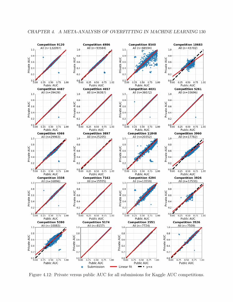
CHAPTER 4. A META-ANALYSIS OF OVERFITTING IN MACHINE LEARNING 130
Submission Linear fit y=x
Figure 4.12: Private versus public AUC for all submissions for Kaggle AUC competitions.

CHAPTER 4. A META-ANALYSIS OF OVERFITTING IN MACHINE LEARNING 131
Submission Linear fit y=x
Figure 4.12: Private versus public AUC for all submissions for Kaggle AUC competitions.

CHAPTER 4. A META-ANALYSIS OF OVERFITTING IN MACHINE LEARNING 132
4.8.2.4 AUC: top 10% of submissions

CHAPTER 4. A META-ANALYSIS OF OVERFITTING IN MACHINE LEARNING 133
Submission Linear fit y=x
Figure 4.13: Private versus public accuracy for top 10% of submissions for Kaggle AUCcompetitions.
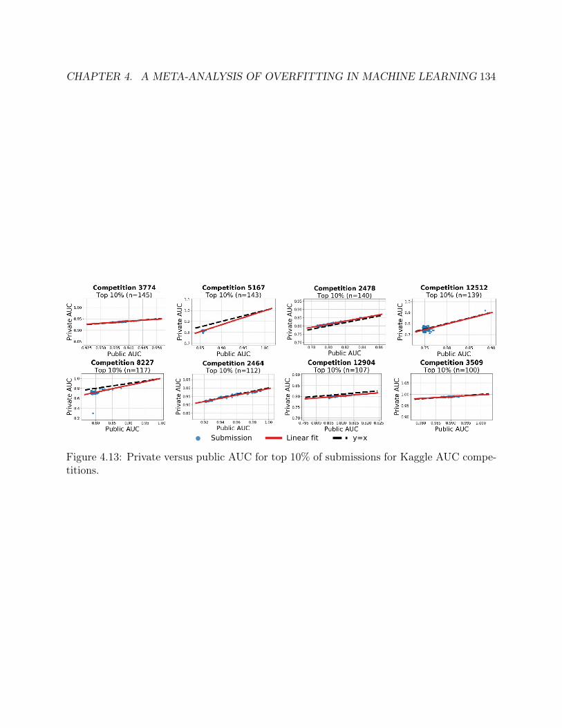
CHAPTER 4. A META-ANALYSIS OF OVERFITTING IN MACHINE LEARNING 134
Submission Linear fit y=x
Figure 4.13: Private versus public AUC for top 10% of submissions for Kaggle AUC compe-titions.

CHAPTER 4. A META-ANALYSIS OF OVERFITTING IN MACHINE LEARNING 135
4.8.3 Map@K
4.8.3.1 Map@K: competition info
Table 4.4: Competitions scored with MAP@K with greater than 1000 submissions. npublic isthe size of the public test set and nprivate is the size of the private test set. N/A means thatwe could not access the competition data to compute the dataset sizes.
MAP@K
ID Name # Sub. npublic nprivate
4481 Coupon Purchase Prediction 18,487 650 1,5155056 Expedia Hotel Recommendations 22,713 834,321 1,693,9235186 Facebook V: Predicting Check Ins 15,127 4,445,370 4,445,3695497 Outbrain Click Prediction 6,654 9,667,549 22,557,6135558 Santander Product Recommendation 28,773 278,884 650,7316818 Humpback Whale Identification 37,529 1,592 6,3687666 CS5785 Fall 2017 Final Exam 3,898 1,000 1,0008396 Google Landmark Retrieval Challenge 3,123 0 117,7048857 Recipient prediction 2018 1,154 1,000 1,0008900 Freesound General-Purpose Audio Tagging Challenge 5,684 282 9,11810200 Quick, Draw! Doodle Recognition Challenge 21,407 10,098 102,10112088 CS5785 Fall 2018 Final 1,877 1,000 1,000
4.8.3.2 Map@K: outlier competitions
We did not observe any MAP@K competitions which exhibit a linear fit that poorly approx-imates the y = x diagonal line (see Section 4.8.3.3).

CHAPTER 4. A META-ANALYSIS OF OVERFITTING IN MACHINE LEARNING 136
4.8.3.3 Map@K: all submissions
Submission Linear fit y=x
Figure 4.14: Private versus public MAP@K for all submissions for Kaggle MAP@K compe-titions.

CHAPTER 4. A META-ANALYSIS OF OVERFITTING IN MACHINE LEARNING 137
4.8.3.4 Map@K: top 10% of submissions
Submission Linear fit y=x
Figure 4.15: Private versus public MAP@K for top 10% of submissions for Kaggle MAP@Kcompetitions.

CHAPTER 4. A META-ANALYSIS OF OVERFITTING IN MACHINE LEARNING 138
4.8.4 MulticlassLoss
4.8.4.1 MulticlassLoss: competition info
Table 4.5: Competitions scored with MulticlassLoss with greater than 1000 submissions.npublic is the size of the public test set and nprivate is the size of the private test set. N/Ameans that we could not access the competition data to compute the dataset sizes.
MulticlassLoss
ID Name # Sub. npublic nprivate
4521 Right Whale Recognition 4,789 N/A N/A4588 Telstra Network Disruptions 19,603 3,240 7,9314654 Walmart Recruiting: Trip Type Classification 13,135 18,629 43,4675048 State Farm Distracted Driver Detection 25,591 N/A N/A5340 TalkingData Mobile User Demographics 24,631 33,621 78,4505568 The Nature Conservancy Fisheries Monitoring 2,100 N/A N/A5590 Two Sigma Connect: Rental Listing Inquiries 47,044 N/A N/A6243 Intel & MobileODT Cervical Cancer Screening 1,367 N/A N/A6841 Personalized Medicine: Redefining Cancer Treatment 3,056 N/A N/A7516 Spooky Author Identification 10,640 2,518 5,874
4.8.4.2 MulticlassLoss: outlier competitions
For MulticlassLoss, we investigated competitions whose linear fit was a bad approximationto the diagonal y = x line. We first identified these competitions using visual inspection ofthe plots in Section 4.8.4.3.
By reading the Kaggle forums and the description of the dataset construction, we wereable to determine a possible cause of overfitting for most of the outlier competitions. Inmost cases, the competition hosts did not create the public and private test splits in a trulyi.i.d. manner, and competitiors were able to exploit the difference in distribution. In othercases, the size of the test set was extremely small. The list of outlier competitions andcorresponding cause of overfitting follow. We also include links to relevant descriptions ofthe data or discussions on the Kaggle forums.
• Competition 6243: Intel & MobileODT Cervical Cancer Screening The testset was released in two stages. https://www.kaggle.com/c/intel-mobileodt-cervical-cancer-screening/data
• Competition 6841: Personalized Medicine: Redefining Cancer TreatmentThe test set was released in two stages because a team discovered the test data from

CHAPTER 4. A META-ANALYSIS OF OVERFITTING IN MACHINE LEARNING 139
Stage 1, including labels, on a public website. https://www.kaggle.com/c/msk-redefining-cancer-treatment/discussion/36383#latest-223033
• Competition 5568: The Nature Conservancy Fisheries Monitoring The testset was released in two stages. https://www.kaggle.com/c/the-nature-conservancy-fisheries-monitoring/data

CHAPTER 4. A META-ANALYSIS OF OVERFITTING IN MACHINE LEARNING 140
4.8.4.3 MulticlassLoss: all submissions
Submission Linear fit y=x
Figure 4.16: Private versus public MulticlassLoss for all submissions for Kaggle Multiclass-Loss competitions.

CHAPTER 4. A META-ANALYSIS OF OVERFITTING IN MACHINE LEARNING 141
4.8.4.4 MulticlassLoss: top 10% of submissions
Submission Linear fit y=x
Figure 4.17: Private versus public MulticlassLoss for top 10% of submissions for KaggleMulticlassLoss competitions.

CHAPTER 4. A META-ANALYSIS OF OVERFITTING IN MACHINE LEARNING 142
4.8.5 LogLoss
4.8.5.1 LogLoss: competition info
LogLoss
ID Name # Sub. npublic nprivate
2780 Predicting a Biological Response 8,843 625 1,8762984 Practice Fusion Diabetes Classification 2,200 1,245 3,7343377 ICDAR2013 - Gender Prediction from Handwriting 1,884 286 4863934 Display Advertising Challenge 8,640 1,208,427 4,833,7083984 Tradeshift Text Classification 5,659 163,525 381,5574120 Click-Through Rate Prediction 31,019 915,493 3,661,9724438 Avito Context Ad Clicks 5,951 2,344,909 5,471,4534852 BNP Paribas Cardif Claims Management 54,519 37,750 76,6434862 March Machine Learning Mania 2016 1,054 N/A N/A6004 Data Science Bowl 2017 1,694 N/A N/A6277 Quora Question Pairs 53,927 140,748 2,205,0487163 WSDM - KKBox’s Churn Prediction Challenge 6,256 N/A N/A7380 Statoil/C-CORE Iceberg Classifier Challenge 42,936 N/A N/A7823 Attrition de clientes 1,911 N/A N/A8310 Google Cloud & NCAA R© ML Competition 2018-Men’s 1,660 N/A N/A
Table 4.6: Competitions scored with LogLoss with greater than 1000 submissions. npublic isthe size of the public test set and nprivate is the size of the private test set. N/A means thatwe could not access the competition data to compute the dataset sizes.
4.8.5.2 LogLoss: outlier competitions
For LogLoss, we observed one competition (Competition 6004: Data Science Bowl 2017)whose linear fit was a bad approximation the diagonal y = x line. The competition showsapproximately 13 outliers when looking at the scatter plot for the top 10% of submissions(see Figure 4.19).
The competition is unique in two aspects: first, the competition used two stages withseparate test sets released at different times and second, participants were allowed to useexternal data. Participants were eventually given all the labels to the Stage 1 test data, butthe Stage 2 test data was different in distribution from the Stage 1 test data (see https://www.kaggle.com/c/data-science-bowl-2017/discussion/31383#latest-174302). Itis unclear whether the final private test data was generated from an i.i.d. split with eitherthe Stage 1 test data or the Stage 2 data. Moreover, training the model on external dataviolates our assumption that the models were only trained and evaluated on i.i.d. data.

CHAPTER 4. A META-ANALYSIS OF OVERFITTING IN MACHINE LEARNING 143
4.8.5.3 LogLoss: all submissions
Submission Linear fit y=x
Figure 4.18: Private versus public LogLoss for all submissions for Kaggle LogLoss competi-tions.

CHAPTER 4. A META-ANALYSIS OF OVERFITTING IN MACHINE LEARNING 144
4.8.5.4 LogLoss: top 10% of submissions
Submission Linear fit y=x
Figure 4.19: Private versus public LogLoss for top 10% of submissions for Kaggle LogLosscompetitions.

CHAPTER 4. A META-ANALYSIS OF OVERFITTING IN MACHINE LEARNING 145
4.8.6 Mean score differences over time
Figure 4.20: Mean score differences (across all pre-deadline submissions) versus competitionend date for all classification evaluation metrics with at least 10 competitions with at least1000 submissions each. Score difference is public minus private for metrics where a higherscore is better (AUC, CategorizationAccuracy (included in the main text), and MAP@K) andprivate minus public for metrics where a lower score is better (LogLoss and MulticlassLoss).Blue dots show InClass competitions and orange dots show all other competition types(Featured, Research, Getting Started, and Playground).

146
Chapter 5
Conclusion
In this thesis, we empirically evaluated key theoretical pillars of machine learning surroundinggeneralization and overfitting in order to better understand machine learning robustness. Weshowed that the choice of optimization algorithm can influence the generalization error of atrained model and demonstrated that adaptive gradient methods frequently find solutionswith worse generalization error than stochastic gradient descent. We then turned to the metaquestion of whether the test error itself is a realiable measurement of generalization error.While the prevailing concern is that test set reuse leads to overfitting and overly optimisticmeasurements of generalization error, we saw little evidence of overfitting in both machinelearning benchmarks and competitions. Instead, we demonstrated that machine learningclassifiers are extremely brittle to small, benign distribution shifts. Overall, designing modelsthat still work in dynamic environments remains a key challenge for robust machine learning.
5.1 Future WorkThis thesis highlights many opportunities for future work, which we outline below.
Empirically understanding overfitting There are multiple directions for empiricallyunderstanding overfitting in more detail. Our analysis of the Meta-Kaggle dataset in Chapter4 focused on classification competitions, but Kaggle also hosts many regression competitions.Is there more adaptive overfitting in regression? Answering this question will likely requireaccess to the individual predictions of the Kaggle submissions to appropriately handle outliersubmissions. In addition, there are still questions among the classification competitions. Forinstance, one refinement of our analysis here is to obtain statistical measures of uncertaintyfor competitions evaluated with metrics such as AUC (which will also require a more fine-grained version of the Kaggle data). Finally, another important question is whether othercompetition platforms such as CodaLab [11] or EvalAI [97] also show few signs of adaptiveoverfitting.

CHAPTER 5. CONCLUSION 147
Measuring Human Accuracy. One interesting question is whether our new test sets arealso harder for humans. As a first step in this direction, our human accuracy experimenton CIFAR-10 (see Section 3.5.2.5) shows that average human performance is not affectedsignificantly by the distribution shift between the original and new images that are mostdifficult for the models. This suggests that the images are only harder for the trained modelsand not for humans. But a more comprehensive understanding of the human baseline willrequire additional human accuracy experiments on both CIFAR-10 and ImageNet.
Characterizing the Distribution Gap. Why do the classification models in our Ima-geNet and CIFAR-10 testbed perform worse on the new test sets? The selection frequencyexperiments in Section 3.4 suggest that images selected less frequently by the MTurk work-ers are harder for the models. However, the selection frequency analysis does not explainwhat aspects of the images make them harder. Candidate hypotheses are object size, specialfilters applied to the images (black & white, sepia, etc.), or unusual object poses. Exploringwhether there is a succinct description of the difference between the original and new testdistributions is an interesting direction for future work.
Learning More Robust Models. An overarching goal is to make classification modelsmore robust to small variations in the data. If the change from the original to our newtest sets can be characterized accurately, techniques such as data augmentation or robustoptimization may be able to close some of the accuracy gap. Otherwise, one possible approachcould be to gather particularly hard examples from Flickr or other data sources and expandthe training set this way. However, it may also be necessary to develop entirely novelapproaches to image classification.
Building Further Test Sets. The dominant paradigm in machine learning is to evaluatethe performance of a classification model on a single test set per benchmark. Our resultssuggest that this is not comprehensive enough to characterize the reliability of current models.To understand their generalization abilities more accurately, new test data from varioussources may be needed. One intriguing question here is whether accuracy on other test setswill also follow a linear function of the original test accuracy.
Suggestions For Future Datasets. We found that it is surprisingly difficult to create anew test set that matches the distribution of an existing dataset. Based on our experiencewith this process, we provide some suggestions for improving machine learning datasets inthe future:
• Code release. It is hard to fully document the dataset creation process in a paperbecause it involves a long list of design choices. Hence it would be beneficial forreproducibility efforts if future dataset papers released not only the data but also allcode used to create the datasets.

CHAPTER 5. CONCLUSION 148
• Annotator quality. Our results show that changes in the human annotation processcan have significant impact on the difficulty of the resulting datasets. To better under-stand the quality of human annotations, it would be valuable if authors conducted astandardized test with their annotators (e.g., classifying a common set of images) andincluded the results in the description of the dataset. Moreover, building variants ofthe test set with different annotation processes could also shed light on the variabilityarising from this data cleaning step.
• “Super hold-out”. Having access to data from the original CIFAR-10 and ImageNetdata collection could have clarified the cause of the accuracy drops in our experiments.By keeping an additional test set hidden for multiple years, future benchmarks couldexplicitly test for adaptive overfitting after a certain time period.
• Simpler tasks for humans. The large number of classes and fine distinctions betweenthem make ImageNet a particularly hard problem for humans without special training.While classifying a large variety of objects with fine-grained distinctions is an importantresearch goal, there are also trade-offs. Often it becomes necessary to rely on imageswith high annotator agreement to ensure correct labels, which in turn leads to biasby excluding harder images. Moreover, the large number of classes causes difficultieswhen characterizing human performance. So an alternative approach for a datasetcould be to choose a task that is simpler for humans in terms of class structure (fewerclasses, clear class boundaries), but contains a larger variety of object poses, lightingconditions, occlusions, image corruptions, etc.
• Test sets with expert annotations. Compared to building a full training set, atest set requires a smaller number of human annotations. This makes it possible toemploy a separate labeling process for the test set that relies on more costly expertannotations. While this violates the assumption that train and test splits are i.i.d.from the same distribution, the expert labels can also increase quality both in termsof correctness and example diversity.
Finally, we emphasize that our recommendations here should not be seen as flaws inCIFAR-10 or ImageNet. Both datasets were assembled in the late 2000s for an accuracyregime that is very different from the state-of-the-art now. Over the past decade, especiallyImageNet has successfully guided the field to increasingly better models, thereby clearlydemonstrating the immense value of this dataset. But as models have increased in accuracyand our reliability expectations have grown accordingly, it is now time to revisit how wecreate and utilize datasets in machine learning.

149
Bibliography
[1] Alex Berg. Personal communication. 2018.
[2] Battista Biggio and Fabio Roli. “Wild Patterns: Ten Years After the Rise of Adver-sarial Machine Learning”. In: Pattern Recognition (2018). https://arxiv.org/abs/1712.03141.
[3] Avrim Blum and Moritz Hardt. “The Ladder: A Reliable Leaderboard for MachineLearning Competitions”. In: International Conference on Machine Learning (ICML).http://arxiv.org/abs/1502.04585. 2015.
[4] Avrim Blum and Moritz Hardt. “The Ladder: A Reliable Leaderboard for MachineLearning Competitions”. In: International Conference on Machine Learning (ICML).2015.
[5] Tianqi Chen and Carlos Guestrin. “XGBoost: A Scalable Tree Boosting System”. In:International Conference on Knowledge Discovery and Data Mining (KDD). 2016.
[6] Yunpeng Chen et al. “Dual path networks”. In: Neural Information Processing Systems(NIPS). https://arxiv.org/abs/1707.01629. 2017.
[7] Do Kook Choe and Eugene Charniak. “Parsing as Language Modeling”. In: Proceed-ings of the 2016 Conference on Empirical Methods in Natural Language Processing,EMNLP 2016, Austin, Texas, USA, November 1-4, 2016. Ed. by Jian Su, Xavier Car-reras, and Kevin Duh. The Association for Computational Linguistics, 2016, pp. 2331–2336. url: http://aclweb.org/anthology/D/D16/D16-1257.pdf.
[8] François Chollet. “Xception: Deep learning with depthwise separable convolutions”.In: Conference on Computer Vision and Pattern Recognition (CVPR). https://arxiv.org/abs/1610.02357. 2017.
[9] Stephane Clinchant et al. “XRCE’s participation to ImagEval”. http://citeseerx.ist.psu.edu/viewdoc/download?doi=10.1.1.102.6670&rep=rep1&type=pdf.2007.
[10] Adam Coates, Andrew Ng, and Honglak Lee. “An analysis of single-layer networks inunsupervised feature learning”. In: Conference on Artificial Intelligence and Statistics(AISTATS). http://proceedings.mlr.press/v15/coates11a.html. 2011.
[11] CodaLab. https://competitions.codalab.org/competitions/.

BIBLIOGRAPHY 150
[12] James Cross and Liang Huang. “Span-Based Constituency Parsing with a Structure-Label System and Provably Optimal Dynamic Oracles”. In: Proceedings of the 2016Conference on Empirical Methods in Natural Language Processing, Austin, Texas.Ed. by Jian Su, Xavier Carreras, and Kevin Duh. The Association for ComputationalLinguistics, 2016, pp. 1–11. url: http://aclweb.org/anthology/D/D16/D16-1001.pdf.
[13] Ekin D. Cubuk et al. “AutoAugment: Learning Augmentation Policies from Data”.https://arxiv.org/abs/1805.09501. 2018.
[14] Jia Deng. “Large Scale Visual Recognition”. ftp : / / ftp . cs . princeton . edu /techreports/2012/923.pdf. PhD thesis. Princeton University, 2012.
[15] Jia Deng et al. “ImageNet: A large-scale hierarchical image database”. In: Conferenceon Computer Vision and Pattern Recognition (CVPR). http://www.image-net.org/papers/imagenet_cvpr09.pdf. 2009.
[16] Terrance DeVries and Graham W Taylor. “Improved regularization of convolutionalneural networks with Cutout”. https://arxiv.org/abs/1708.04552. 2017.
[17] Simon S Du et al. “Gradient descent finds global minima of deep neural networks”.In: International Conference on Machine Learning (ICML). 2019.
[18] Simon S Du et al. “Gradient descent provably optimizes over-parameterized neuralnetworks”. In: (2019).
[19] John C. Duchi, Elad Hazan, and Yoram Singer. “Adaptive Subgradient Methods forOnline Learning and Stochastic Optimization”. In: Journal of Machine Learning Re-search 12 (2011), pp. 2121–2159. url: http://dl.acm.org/citation.cfm?id=2021068.
[20] Cynthia Dwork et al. “Preserving statistical validity in adaptive data analysis”. In:ACM symposium on Theory of computing (STOC). 2015.
[21] Logan Engstrom et al. “A Rotation and a Translation Suffice: Fooling CNNs withSimple Transformations”. http://arxiv.org/abs/1712.02779. 2017.
[22] Logan Engstrom et al. “Exploring the Landscape of Spatial Robustness”. In: Interna-tional Conference on Machine Learning (ICML). 2019.
[23] Mark Everingham et al. “The Pascal Visual Object Classes (VOC) Challenge”. In:International Journal of Computer Vision (2010). http://dx.doi.org/10.1007/s11263-009-0275-4.
[24] Alhussein Fawzi and Pascal Frossard. “Manitest: Are classifiers really invariant?” In:British Machine Vision Conference (BMVC). https://arxiv.org/abs/1507.06535.2015.

BIBLIOGRAPHY 151
[25] Li Fei-Fei, Rob Fergus, and Pietro Perona. “Learning Generative Visual Models fromFew Training Examples: An Incremental Bayesian Approach Tested on 101 ObjectCategories”. In: Computer Vision and Image Understanding (2007). http://dx.doi.org/10.1016/j.cviu.2005.09.012.
[26] Vitaly Feldman, Roy Frostig, and Moritz Hardt. “The advantages of multiple classesfor reducing overfitting from test set reuse”. In: International Conference on MachineLearning (ICML) (2019).
[27] Kunihiko Fukushima. “Neocognitron: A self-organizing neural network model for amechanism of pattern recognition unaffected by shift in position”. In: Biological Cy-bernetics. 1980.
[28] Xavier Gastaldi. “Shake-shake regularization”. https://arxiv.org/abs/1705.07485. 2017.
[29] Robert Geirhos et al. “Generalisation in humans and deep neural networks”. In: Ad-vances in Neural Information Processing Systems (NeurIPS). http://papers.nips.cc/paper/7982-generalisation-in-humans-and-deep-neural-networks.pdf.2018.
[30] Ben Hamner. “Popular Datasets Over Time”. Accessed: 2019-01-22. 2017.
[31] Dongyoon Han, Jiwhan Kim, and Junmo Kim. “Deep pyramidal residual networks”.In: Conference on Computer Vision and Pattern Recognition (CVPR). https://arxiv.org/abs/1610.02915. 2017.
[32] Kaiming He et al. “Deep residual learning for image recognition”. In: Conference onComputer Vision and Pattern Recognition (CVPR). https://arxiv.org/abs/1512.03385. 2016.
[33] Kaiming He et al. “Delving Deep into Rectifiers: Surpassing Human-Level Perfor-mance on ImageNet Classification”. In: International Conference on Computer Vision(ICCV). https://arxiv.org/abs/1502.01852. 2015.
[34] Kaiming He et al. “Identity mappings in deep residual networks”. In: European Con-ference on Computer Vision (ECCV). https://arxiv.org/abs/1603.05027. 2016.
[35] Dan Hendrycks and Thomas Dietterich. “Benchmarking Neural Network Robustnessto Common Corruptions and Perturbations”. In: International Conference on Learn-ing Representations (ICLR). https://arxiv.org/abs/1807.01697. 2019.
[36] Sepp Hochreiter and Jürgen Schmidhuber. “Flat minima”. In: Neural Computation9.1 (1997), pp. 1–42.
[37] Hossein Hosseini and Radha Poovendran. “Semantic Adversarial Examples”. In: Con-ference on Computer Vision and Pattern Recognition (CVPR) Workshops. https://arxiv.org/abs/1804.00499. 2018.
[38] Andrew G Howard et al. “Mobilenets: Efficient convolutional neural networks formobile vision applications”. https://arxiv.org/abs/1704.04861. 2017.

BIBLIOGRAPHY 152
[39] Jie Hu, Li Shen, and Gang Sun. “Squeeze-and-excitation networks”. In: Conferenceon Computer Vision and Pattern Recognition (CVPR). https://arxiv.org/abs/1709.01507. 2018.
[40] Gao Huang et al. “Densely connected convolutional networks”. In: Conference onComputer Vision and Pattern Recognition (CVPR). https: //arxiv .org/ abs /1608.06993. 2017.
[41] Forrest N. Iandola et al. “SqueezeNet: AlexNet-level accuracy with 50x fewer param-eters and <0.5MB model size”. https://arxiv.org/abs/1602.07360. 2016.
[42] Sergey Ioffe and Christian Szegedy. “Batch normalization: Accelerating deep networktraining by reducing internal covariate shift”. In: International Conference on MachineLearning (ICML). https://arxiv.org/abs/1502.03167. 2015.
[43] Phillip Isola et al. “Image-to-Image Translation with Conditional Adversarial Net-works”. arXiv:1611.07004. 2016.
[44] Kaggle. https://www.kaggle.com/.
[45] Can Kanbak, Seyed-Mohsen Moosavi-Dezfooli, and Pascal Frossard. “Geometric Ro-bustness of Deep Networks: Analysis and Improvement”. In: Conference on ComputerVision and Pattern Recognition (CVPR). https://arxiv.org/abs/1711.09115.2018.
[46] Andrej Karparthy. A Peek at Trends in Machine Learning. https://medium.com/@karpathy/a-peek-at-trends-in-machine-learning-ab8a1085a106. Accessed:2017-05-17.
[47] Andrej Karpathy. “Lessons learned from manually classifying CIFAR-10”. http://karpathy.github.io/2011/04/27/manually-classifying-cifar10/. 2011.
[48] Kenji Kawaguchi, Leslie Pack Kaelbling, and Yoshua Bengio. “Generalization in deeplearning”. https://arxiv.org/abs/1710.05468. 2017.
[49] Nitish Shirish Keskar et al. “On large-batch training for deep learning: Generalizationgap and sharp minima”. In: The International Conference on Learning Representa-tions (ICLR). 2017.
[50] D.P. Kingma and J. Ba. “Adam: A Method for Stochastic Optimization”. In: TheInternational Conference on Learning Representations (ICLR) (2015).
[51] Simon Kornblith, Jonathon Shlens, and Quoc V. Le. “Do Better ImageNet ModelsTransfer Better?” http://arxiv.org/abs/1805.08974. 2018.
[52] Ivan Krasin et al. “OpenImages: A public dataset for large-scale multi-label and multi-class image classification.” https://storage.googleapis.com/openimages/web/index.html. 2017.
[53] Alex Krizhevsky. “Learning multiple layers of features from tiny images”. https://www.cs.toronto.edu/~kriz/learning-features-2009-TR.pdf. 2009.

BIBLIOGRAPHY 153
[54] Alex Krizhevsky, Ilya Sutskever, and Geoffrey E Hinton. “Imagenet classificationwith deep convolutional neural networks”. In: Advances in Neural Information Pro-cessing Systems (NIPS). https : / / papers . nips . cc / paper / 4824 - imagenet -classification-with-deep-convolutional-neural-networks. 2012.
[55] Fei-Fei Li and Jia Deng. “ImageNet: Where have we been? Where are we going?”http://image-net.org/challenges/talks_2017/imagenet_ilsvrc2017_v1.0.pdf. 2017.
[56] Timothy P Lillicrap et al. “Continuous control with deep reinforcement learning”. In:International Conference on Learning Representations (ICLR). 2016.
[57] Tsung-Yi Lin et al. “Microsoft COCO: Common Objects in Context”. In: EuropeanConference on Computer Vision (ECCV). https://arxiv.org/abs/1405.0312.2014.
[58] Chenxi Liu et al. “Progressive neural architecture search”. In: European Conferenceon Computer Vision (ECCV). https://arxiv.org/abs/1712.00559. 2018.
[59] Shuying Liu and Weihong Deng. “Very deep convolutional neural network based im-age classification using small training sample size”. In: Asian Conference on PatternRecognition (ACPR). https://ieeexplore.ieee.org/document/7486599/. 2015.
[60] Siyuan Ma and Mikhail Belkin. “Diving into the shallows: a computational perspectiveon large-scale shallow learning”. arXiv:1703.10622. 2017.
[61] Aleksander Madry et al. “Towards Deep Learning Models Resistant to AdversarialAttacks”. In: International Conference on Learning Representations (ICLR). https://arxiv.org/abs/1706.06083. 2018.
[62] Jitendra Malik. “Technical Perspective: What Led Computer Vision to Deep Learn-ing?” In: Communications of the ACM (2017). http://doi.acm.org/10.1145/3065384.
[63] Mitchell P. Marcus, Mary Ann Marcinkiewicz, and Beatrice Santorini. “Building aLarge Annotated Corpus of English: The Penn Treebank”. In: COMPUTATIONALLINGUISTICS 19.2 (1993), pp. 313–330.
[64] H. Brendan McMahan and Matthew Streeter. “Adaptive Bound Optimization for On-line Convex Optimization”. In: Proceedings of the 23rd Annual Conference on LearningTheory (COLT). 2010.
[65] George A. Miller. “WordNet: A Lexical Database for English”. In: Communicationsof the ACM (1995). url: http://doi.acm.org/10.1145/219717.219748.
[66] Volodymyr Mnih et al. “Asynchronous methods for deep reinforcement learning”. In:International Conference on Machine Learning (ICML). 2016.
[67] Kevin P. Murphy. Machine Learning: A Probabilistic Perspective. Chapter 1.4.8. TheMIT Press, 2012.

BIBLIOGRAPHY 154
[68] Behnam Neyshabur, Ruslan Salakhutdinov, and Nathan Srebro. “Path-SGD: Path-Normalized Optimization in Deep Neural Networks.” In: Neural Information Process-ing Systems (NIPS). 2015.
[69] Behnam Neyshabur, Ryota Tomioka, and Nathan Srebro. “In Search of the RealInductive Bias: On the Role of Implicit Regularization in Deep Learning”. In: Inter-national Conference on Learning Representations (ICLR). 2015.
[70] Fabian Pedregosa et al. “Scikit-learn: Machine Learning in Python”. In: Journal ofMachine Learning Research (2011).
[71] Florent Perronnin, Jorge Sánchez, and Thomas Mensink. “Improving the Fisher Ker-nel for Large-scale Image Classification”. In: European Conference on Computer Vi-sion (ECCV). 2010. url: https://www.robots.ox.ac.uk/~vgg/rg/papers/peronnin_etal_ECCV10.pdf.
[72] Jean Ponce et al. “Dataset issues in object recognition”. In: Toward Category-LevelObject Recognition. https://link.springer.com/chapter/10.1007/11957959_2.2006.
[73] Joaquin Quionero-Candela et al. Dataset Shift in Machine Learning. The MIT Press,2009.
[74] Maxim Raginsky, Alexander Rakhlin, and Matus Telgarsky. “Non-convex learning viaStochastic Gradient Langevin Dynamics: a nonasymptotic analysis”. arXiv:1702.03849. 2017.
[75] Ali Rahimi and Benjamin Recht. “Weighted Sums of Random Kitchen Sinks: Re-placing minimization with randomization in learning”. In: Advances in Neural In-formation Processing Systems (NIPS). https://papers.nips.cc/paper/3495-weighted-sums-of-random-kitchen-sinks-replacing-minimization-with-randomization-in-learning. 2009.
[76] Esteban Real et al. “Regularized Evolution for Image Classifier Architecture Search”.http://arxiv.org/abs/1802.01548. 2018.
[77] Benjamin Recht, Moritz Hardt, and Yoram Singer. “Train faster, generalize better:Stability of stochastic gradient descent”. In: Proceedings of the International Confer-ence on Machine Learning (ICML). 2016.
[78] Benjamin Recht et al. “Do ImageNet Classifiers Generalize to ImageNet?” In: Inter-national Conference on Machine Learning (ICML). 2019.
[79] Scott Reed et al. “Generative adversarial text to image synthesis”. In: Proceedings ofThe International Conference on Machine Learning (ICML). 2016.
[80] Aaron Roth and Adam Smith. Lectures notes “The Algorithmic Foundations of Adap-tive Data Analysis”. https://adaptivedataanalysis.com/. 2017.
[81] Olga Russakovsky et al. “ImageNet large scale visual recognition challenge”. In: Inter-national Journal of Computer Vision (2015). https://arxiv.org/abs/1409.0575.

BIBLIOGRAPHY 155
[82] Shibani Santurkar et al. “How Does Batch Normalization Help Optimization?” In:Advances in Neural Information Processing Systems 31. 2018. url: http://papers.nips.cc/paper/7515-how-does-batch-normalization-help-optimization.pdf.
[83] Shai Shalev-Shwartz and Shai Ben-David. Understanding Machine Learning: FromTheory to Algorithms. Cambridge University Press, 2014.
[84] Karen Simonyan and Andrew Zisserman. “Very deep convolutional networks for large-scale image recognition”. https://arxiv.org/abs/1409.1556. 2014.
[85] Ilya Sutskever et al. “On the importance of initialization and momentum in deep learn-ing”. In: Proceedings of the International Conference on Machine Learning (ICML).2013.
[86] Christian Szegedy et al. “Going deeper with convolutions”. In: Conference on Com-puter Vision and Pattern Recognition (CVPR). https://arxiv.org/abs/1409.4842v1. 2015.
[87] Christian Szegedy et al. “Inception-v4, Inception-Resnet and the impact of residualconnections on learning”. In: Conference On Artificial Intelligence (AAAI). https://arxiv.org/abs/1602.07261. 2017.
[88] Christian Szegedy et al. “Intriguing properties of neural networks”. In: InternationalConference on Learning Representations (ICLR). http://arxiv.org/abs/1312.6199. 2013.
[89] Christian Szegedy et al. “Rethinking the Inception architecture for computer vision”.In: Conference on Computer Vision and Pattern Recognition (CVPR). https://arxiv.org/abs/1512.00567. 2016.
[90] Christian Szegedy et al. “Rethinking the inception architecture for computer vision”.In: Proceedings of the IEEE Conference on Computer Vision and Pattern Recognition(CVPR). 2016.
[91] T. Tieleman and G. Hinton. Lecture 6.5—RmsProp: Divide the gradient by a runningaverage of its recent magnitude. COURSERA: Neural Networks for Machine Learning.2012.
[92] Antonio Torralba and Alexei A. Efros. “Unbiased look at dataset bias”. In: Conferenceon Computer Vision and Pattern Recognition (CVPR). http://people.csail.mit.edu/torralba/publications/datasets_cvpr11.pdf. 2011.
[93] Antonio Torralba, Rob Fergus, and William. T. Freeman. “80 Million Tiny Images: ALarge Data Set for Nonparametric Object and Scene Recognition”. In: IEEE Trans-actions on Pattern Analysis and Machine Intelligence (2008). https://ieeexplore.ieee.org/document/4531741/.
[94] Zhou Wang et al. “Image quality assessment: from error visibility to structural sim-ilarity”. In: IEEE Transactions on Image Processing (2004). http://www.cns.nyu.edu/pub/lcv/wang03-preprint.pdf.

BIBLIOGRAPHY 156
[95] Chaowei Xiao et al. “Spatially Transformed Adversarial Examples”. In: InternationalConference on Learning Representations (ICLR). https://arxiv.org/abs/1801.02612. 2018.
[96] Saining Xie et al. “Aggregated residual transformations for deep neural networks”. In:Conference on Computer Vision and Pattern Recognition (CVPR). https://arxiv.org/abs/1611.05431. 2017.
[97] Deshraj Yadav et al. “EvalAI: Towards Better Evaluation Systems for AI Agents”.2019. url: http://arxiv.org/abs/1902.03570.
[98] Yoshihiro Yamada, Masakazu Iwamura, and Koichi Kise. “ShakeDrop regularization”.https://arxiv.org/abs/1802.02375. 2018.
[99] Benjamin Z. Yao, Xiong Yang, and Song-Chun Zhu. “Introduction to a large-scalegeneral purpose ground truth database: methodology, annotation tool and bench-marks”. In: Energy Minimization Methods in Computer Vision and Pattern Recogni-tion (EMMCVPR). https://link.springer.com/chapter/10.1007/978-3-540-74198-5_14. 2007.
[100] Yuan Yao, Lorenzo Rosasco, and Andrea Caponnetto. “On early stopping in gradientdescent learning”. In: Constructive Approximation 26.2 (2007), pp. 289–315.
[101] Sergey Zagoruyko. Torch Blog. http://torch.ch/blog/2015/07/30/cifar.html.2015.
[102] Sergey Zagoruyko and Nikos Komodakis. “Wide residual networks”. In: British Ma-chine Vision Conference (BMVC). https://arxiv.org/abs/1605.07146. 2016.
[103] Xingcheng Zhang et al. “Polynet: A pursuit of structural diversity in very deep net-works”. In: Conference on Computer Vision and Pattern Recognition (CVPR). https://arxiv.org/abs/1611.05725. 2017.
[104] Barret Zoph et al. “Learning transferable architectures for scalable image recognition”.In: Conference on Computer Vision and Pattern Recognition (CVPR). https://arxiv.org/abs/1707.07012. 2018.
[105] Tijana Zrnic and Moritz Hardt. “Natural Analysts in Adaptive Data Analysis”. In:International Conference on Machine Learning (ICML) (2019).