LATE WITH GENERALIZATION FOR DEEP NEU - OpenReview

Under review as a conference paper at ICLR 2022

WHY FLATNESS DOES AND DOES NOT CORRE-LATE WITH GENERALIZATION FOR DEEP NEU-RAL NETWORKS

Anonymous authorsPaper under double-blind review

ABSTRACT

The intuition that local flatness of the loss landscape is correlated with bettergeneralization for deep neural networks (DNNs) has been explored for decades,spawning many different flatness measures. Recently, this link with generalizationhas been called into question by a demonstration that many measures of flatnessare vulnerable to parameter re-scaling which arbitrarily changes their value withoutchanging neural network outputs. Here we show that, in addition, some popularvariants of SGD such as Adam and Entropy-SGD, can also break the flatness-generalization correlation. As an alternative to flatness measures, we use a functionbased picture and propose using the log of Bayesian prior upon initialization,logP (f), as a predictor of the generalization when a DNN converges on functionf after training to zero error. The prior is directly proportional to the Bayesianposterior for functions that give zero error on a training set. For the case of imageclassification, we show that logP (f) is a significantly more robust predictor ofgeneralization than flatness measures are. Whilst local flatness measures fail underparameter re-scaling, the prior/posterior, which is global quantity, remains invariantunder re-scaling. Moreover, the correlation with generalization as a function ofdata complexity remains good for different variants of SGD.

1 INTRODUCTION

Among the most important theoretical questions in the field of deep learning are: 1) What charac-terizes functions that exhibit good generalization?, and 2) Why do overparameterized deep neuralnetworks (DNNs) converge to this small subset of functions that do not overfit? Perhaps the mostpopular hypothesis is that good generalization performance is linked to flat minima. In pioneeringworks (Hinton & van Camp, 1993; Hochreiter & Schmidhuber, 1997), the minimum descriptionlength (MDL) principle (Rissanen, 1978) was invoked to argue that since flatter minima require lessinformation to describe, they should generalize better than sharp minima. Most measures of flatnessapproximate the local curvature of the loss surface, typically defining flatter minima to be those withsmaller values of the Hessian eigenvalues (Keskar et al., 2016; Wu et al., 2017; Zhang et al., 2018;Sagun et al., 2016; Yao et al., 2018).

Another commonly held belief is that stochastic gradient descent (SGD) is itself biased towardsflatter minima, and that this inductive bias helps explain why DNNs generalize so well (Keskar et al.,2016; Jastrzebski et al., 2018; Wu et al., 2017; Zhang et al., 2018; Yao et al., 2018; Wei & Schwab,2019; Maddox et al., 2020). For example Keskar et al. (2016) developed a measure of flatnessthat they found correlated with improved generalization performance when decreasing batch size,suggesting that SGD is itself biased towards flatter minima. We note that others (Goyal et al., 2017;Hoffer et al., 2017; Smith et al., 2017; Mingard et al., 2021a) have argued that the effect of batch sizecan be compensated by changes in learning rate, complicating some conclusions from Keskar et al.(2016). Nevertheless, the argument that SGD is somehow itself biased towards flat minima remainswidespread in the literature.

In an important critique of local flatness measures, Dinh et al. (2017) pointed out that DNNs withReLU activation can be re-parameterized through a simple parameter-rescaling transformation.

Tα : (w1,w2) 7→(αw1, α

−1w2

)(1)

1


where w1 are the weights between an input layer and a single hidden layer, and w2 are the weightsbetween this hidden layer and the outputs. This transformation can be extended to any architecturehaving at least one single rectified network layer. The function that the DNN represents, and thushow it generalizes, is invariant under parameter-rescaling transformations, but the derivatives w.r.t.parameters, and therefore many flatness measures used in the literature, can be changed arbitrarily.Ergo, the correlation between flatness and generalization can be arbitrarily changed.

Several recent studies have attempted to find "scale invariant" flatness metrics (Petzka et al., 2019;Rangamani et al., 2019; Tsuzuku et al., 2019). The main idea is to multiply layer-wise Hessianeigenvalues by a factor of ‖wi‖2, which renders the metric immune to layer-wise re-parameterization.While these new metrics look promising experimentally, they are only scale-invariant when thescaling is layer-wise. Other methods of rescaling (e.g. neuron-wise rescaling) can still change themetrics, so this general problem remains unsolved.

1.1 MAIN CONTRIBUTIONS

1. For a series of classic image classification tasks (MNIST and CIFAR-10) we show thatflatness measures change substantially as a function of epochs. Parameter re-scaling canarbitrarily change flatness, but it quickly recovers to a more typical value under furthertraining. We also demonstrate that some variants of SGD exhibit significantly worsecorrelation of flatness with generalization than found for vanilla SGD. In other words popularmeasures of flatness sometimes do and sometimes do not correlate with generalization.This mixed performance problematizes a widely held intuition that DNNs generalize wellfundamentally because SGD or its variants are themselves biased towards flat minima.

2. We next study the correlation of the Bayesian prior P (f) with the generalization performanceof a DNN that converges to that function f . This prior is the weighted probability of obtainingfunction f upon random sampling of parameters. Motivated by a theoretical argumentderived from a non-uniform convergence generalization bound, we show empirically thatlogP (f) correlates robustly with test error, even when local flatness measures miserablyfail, for example upon parameter re-scaling. For discrete input/output problems (such asclassification), P (f) can also be interpreted as the weighted "volume" of parameters thatmap to f . Intuitively, we expect local flatness measures to typically be smaller (flatter)for systems with larger volumes. Nevertheless, there may also be regions of parameterspace where local derivatives and flatness measures vary substantially, even if on averagethey correlate with the volume. Thus flatness measures can be viewed as (imperfect) localmeasures of a more robust predictor of generalization, the volume/prior P (f).

2 DEFINITIONS AND NOTATION

2.1 SUPERVISED LEARNING

For a typical supervised learning problem, the inputs live in an input domain X , and the outputsbelong to an output space Y . For a data distribution D on the set of input-output pairs X × Y , thetraining set S is a sample of m input-output pairs sampled i.i.d. from D, S = {(xi, yi)}mi=1 ∼ Dm,where xi ∈ X and yi ∈ Y . The output of a DNN on an input xi is denoted as yi. Typically aDNN is parameterized by a vector w and trained by minimizing a loss function L : Y × Y → R,which measures differences between the output y ∈ Y and the ground truth output y ∈ Y , byassigning a score L(y, y) which is typically zero when they match, and positive when they don’tmatch. Minimizing the loss typically involves using an optimization algorithm such as SGD ona training set S. The generalization performance of the DNN, which is theoretically defined overthe underlying (typically unknown) data distribution D but is practically measured on a test setE = {(x′i, y′i)}

|E|i=1 ∼ D|E|. For classification problems, the generalization error is practically

measured as ε(E) = 1|E|∑x′i∈E

1[yi 6= y′i], where 1 is the standard indicator function which is onewhen its input is true, and zero otherwise.

2


2.2 FLATNESS MEASURES

Perhaps the most natural way to measure the flatness of minima is to consider the eigenvalue distribu-tion of the Hessian Hij = ∂2L(w)/∂wi∂wj once the learning process has converged (typically to azero training error solution). Here for simplicity we use L(w) instead of L(y, y) as y is parameterizedby w. Sharp minima are characterized by a significant number of large positive eigenvalues λi inthe Hessian, while flat minima are dominated by small eigenvalues. Some care must be used inthis interpretation because it is widely thought that DNNs converge to stationary points that arenot true minima, leading to negative eigenvalues and complicating their use in measures of flatness.Typically, only a subset of the positive eigenvalues are used (Wu et al., 2017; Zhang et al., 2018).Hessians are typically very expensive to calculate. For this reason, Keskar et al. (2016) introduced acomputationally more tractable measure called "sharpness":

Definition 2.1 (Sharpness). Given parameters w′ within a box in parameter space Cζ with sides oflength ζ > 0, centered around a minimum of interest at parameters w, the sharpness of the loss L(w)at w is defined as:

sharpness :=maxw′∈Cζ (L(w

′)− L(w))

1 + L(w)× 100.

In the limit of small ζ, the sharpness relates to the spectral norm of the Hessian (Dinh et al., 2017):

sharpness ≈∥∥∣∣(∇2L(w)

)∣∣∥∥2ζ2

2(1 + L(w))× 100.

The general concept of flatness can be defined as 1/sharpness, and that is how we will interpret thismeasure in the rest of this paper.

2.3 FUNCTIONS AND THE BAYESIAN PRIOR

We first clarify how we represent functions in the rest of paper using the notion of restriction offunctions. A more detailed explanation can be found in appendix C. Here we use binary classificationas an example:

Definition 2.2 (Restriction of functions to C). (Shalev-Shwartz & Ben-David, 2014) Consider aparameterized supervised model, and let the input space be X and the output space be Y , notingY = {0, 1} in binary classification setting. The space of functions the model can express is a(potentially uncountably infinite) set F ⊆ Y |X |. Let C = {c1, . . . , cm} ⊂ X . The restriction of F toC is the set of functions from C to Y that can be derived from functions in F :

FC = {(f (c1) , . . . , f (cm)) : f ∈ F}

where we represent each function from C to Y as a vector in Y |C|.

For example, for binary classification, if we restrict the functions to S + E, then each function inFS+E is represented as a binary string of length |S|+ |E|. In the rest of paper, we simply refer to"functions" when we actually mean the restriction of functions to S + E, except for the Booleansystem in section 5.1 where no restriction is needed. See appendix C for a thorough explanation.

For discrete functions, we next define the prior probability P (f) as

Definition 2.3 (Prior of a function). Given a prior parameter distribution Pw(w) over the parameters,the prior of function f can be defined as:

P (f) :=

∫1[M(w) = f ]Pw(w)dw. (2)

where 1 is an indicator function:1[arg] = 1 if its argument is true or 0 otherwise;M is the parameter-function map whose formal definition is in appendix B. Note that P (f) could also be interpreted as aweighted volume V (f) over parameter space. If Pw(w) is the distribution at initialization, the P (f)is the prior probability of obtaining the function at initialization. We normally use this parameterdistribution when interpreting P (f).

3


Figure 1: Schematic loss landscape for three functions that have zero-error on the training set.It illustrates how the relative sizes of the volumes of their basins of attraction VSGD(fi) correlatewith the volumes V (fi) (or equivalently their priors P (fi)) of the basins, and that, on average, largerV (fi) or P (fi) implies flatter functions, even if flatness can vary locally. Note that the loss L(w) canvary within a region where the DNN achieves zero classification error on S. A similar schematic plotcan be seen in (Mingard et al., 2021b), but here it is more clear that local flatness can be misleading.Note the "error" means the classification error, which is different from the loss.

Remark. Definition 2.3 works in the situation where the spaceX and Y are discrete, where P (f) has aprior probability mass interpretation. This is enough for most image classification tasks. Nevertheless,we can easily extend this definition to the continuous setting, where we can also define a prior densityover functions upon random initialization, with the help of Gaussian Process (GP) (Rasmussen, 2003).For the GP prior see appendix D. However, in this work, we focus exclusively on the classificationsetting, with discrete inputs and outputs.

2.4 LINK BETWEEN THE PRIOR AND THE BAYESIAN POSTERIOR

Due to their high expressivity, DNNs are typically trained to zero training error on the training setS. In this case the Bayesian picture simplifies because if functions are conditioned on zero erroron S, this leads to a simple 0-1 likelihood P (S|f), indicating whether the data is consistent withthe function. Bayesian inference can be used to calculate a Bayesian posterior probability PB(f |S)for each f by conditioning on the data according to Bayes rule. Formally, if S = {(xi, yi)}mi=1corresponds to the set of training pairs, then

PB(f |S) ={P (f)/P (S) if ∀i, f(xi) = yi0 otherwise .

where P (f) is the Bayesian prior and P (S) is called the marginal likelihood or Bayesian evidence.If we define, the training set neutral space NS as all parameters that lead to functions that give zerotraining error on S, then P (S) =

∫NS Pw(w)dw. In other words, it is the total prior probability

of all functions compatible with the training set S (Valle-Pérez et al., 2018; Mingard et al., 2021a).Since P (S) is constant for a given S, PB(f |S) ∝ P (f) for all f consistent with that S.

3 THE CORRELATION BETWEEN THE PRIOR AND GENERALIZATION

This link between the prior and the posterior is important, because it was empirically found in anextensive set of experiments by (Mingard et al., 2021a) that, for popular architectures and data sets,

PB(f |S) ≈ PSGD(f |S), (3)

where PSGD(f |S) is the probability that a DNN trained with SGD converges on function f , whentrained to zero error on S. In other words, to first order, SGD appears to find functions with aprobability predicted by the Bayesian posterior, and thus with probabilities directly proportional toP (f). The authors traced this behaviour to the geometry of the loss landscape, as follows. Somegeneral observations from algorithmic information theory (AIT) (Valle-Pérez et al., 2018) as well

4


as direct calculations (Mingard et al., 2019) predict that the priors of functions should vary overmany orders of magnitude. When this is the case, it is reasonable to expect that the probabilities bywhich an optimizer finds different functions is affected by these large differences. This is relatedto a mechanism identified previously in evolutionary dynamics, where it is called the arrival of thefrequent (Schaper & Louis, 2014). We illustrate this principle in fig. 1 where we intuitively use thelanguage of "volumes". We expect that the relative sizes of the basins of attraction VSGD(f), definedas the set of initial parameters for which a DNN converges to a certain function f , is proportional, tofirst order, to those of the priors P (f) (or equivalently the "volumes"). To second order there are, ofcourse, many other features of a search method and a landscape that affect what functions a DNNconverges on, but when the volumes/priors vary by so many orders of magnitude then we expect thatto first order PSGD(f |S) ≈ PB(f |S) ∝ P (f) = V (f).

Given that the P (f) of a function helps predict how likely SGD is to converge on that function, wecan next ask how P (f) correlates with generalization. Perhaps the simplest argument is that if DNNstrained to zero error are known to generalize well on unseen data, then the probability of convergingon functions that generalize well must be high. The P (f) of these functions must be larger than thepriors of functions that do not generalize well. Can we do better than this rather simplistic argument?One way forward is empirical. Mingard et al. (2021a) showed that log (PB(f |S)) correlates quitetightly with generalization error. These authors also made a theoretical argument based on thePoisson-Binomial nature of the error distribution to explain this log-linear relationship, but thisapproach needs further work.

One of the best overall performing predictors in the literature for generalization performance onclassification tasks is the marginal likelihood PAC-Bayes bound from Valle-Pérez et al. (2018);Valle-Pérez & Louis (2020). It is non-vacuous, relatively tight, and can capture important trends ingeneralization performance with training set size (learning curves), data complexity, and architecturechoice (see also (Liu et al., 2021)). However, the prediction uses the marginal likelihood P (S)defined through a sum over all functions that produce zero error on the training set. Here we areinterested in the generalization properties of single functions. One way around is to use a simplenonuniform bound which to the best of our knowledge was first published in McAllester (1998)as a preliminary theory to the full PAC-Bayes theorems. For any countable function space F , anydistribution P , and for any selection of a training set S of size m under probability distribution D, itcan be proven that for all functions f that give zero training error:

∀D,PS∼Dm[εS,E(f) ≤

ln 1P (f)

+ ln 1δ

m

]≥ 1− δ (4)

for δ ∈ (0, 1). Here we consider a space FS,E of functions with all possible outputs on the inputs ofa specific E and zero error on a specific S; εS,E(f) is the error measured on E + S, which as theerror on S is 0, equals the error on the test set E. This error will converge to the true generalizationerror on all possible inputs as |E| increases. Valle-Pérez & Louis (2020) showed this bound has anoptimal average generalization error when P (f) mimics the probability distribution over functions ofthe learning algorithm. If PSGD(f) ≈ PB(f |S) ∝ P (f), then the best performance of the bound isapproximately when P (f) in eq. (4) is the Bayesian prior P (f). Thus this upper bound on εS,E(f)scales as − log (P (f)).

4 FLATNESS, PRIORS AND GENERALIZATION

The intuition that larger P (f) correlates with greater flatness is common in the literature, seee.g. Hochreiter & Schmidhuber (1997); Wu et al. (2017), where the intuition is also expressed interms of volumes. If volume/P (f) correlates with generalization, we expect flatness should too.Nevertheless, local flatness may still vary significantly across a volume. For example Izmailov et al.(2018) show explicitly that even in the same basin of attraction, there can be flatter and sharperregions. We illustrate this point schematically in fig. 1, where one function clearly has a larger volumeand on average smaller derivatives of the loss w.r.t. the parameters than the others, and so is flatter onaverage. But, there are also local areas within the zero-error region where this correlation does nothold. One of the main hypotheses we will test in this paper is that the correlation between flatnessand generalization can be broken even when the generalization-prior correlation remains robust.

5


Figure 2: The correlation between flatness and the Bayesian prior for the n = 7 Booleansystem. The functions are defined on the full space of 128 possible inputs. The priors P (f) areshown for the 1000 most frequently found functions by SGD from random initialization for a twohidden layer FCN, and correlate well with log(flatness). The function with the largest prior, which isthe most "flat" is the trivial one of all 0s or all 1s. An additional feature is two offset bands caused bya discontinuity of Boolean functions. Most functions shown are mainly 0s or mainly 1s, and the twobands correspond to different number of outliers (e.g. 1s when the majority is 0s).

5 EXPERIMENTAL RESULTS

5.1 PRIOR/VOLUME - FLATNESS CORRELATION FOR BOOLEAN SYSTEM

We first study a model system for Boolean functions of size n = 7, which is small enough to directlymeasure the prior by sampling (Valle-Pérez et al., 2018). There are 27 = 128 possible binary inputs.Since each input is mapped to a single binary output, there are 2128 = 3.4×1034 possible functions f .It is only practically possible to sample the prior P (f) because it is highly biased (Valle-Pérez et al.,2018; Mingard et al., 2019), meaning a subset of functions have priors much higher than average. Fora fully connected network (FCN) with two hidden layers of 40 ReLU units each (which was found tobe sufficiently expressive to represent almost all possible functions) we empirically determined P (f)using 108 random samples of the weights w over an initial Gaussian parameter distribution Pw(w)with standard deviation σw = 1.0 and σb = 0.1.

We also trained our network with SGD using the same initialization and recorded the top-1000most commonly appearing output functions with zero training error on all 128 outputs, and thenevaluated the sharpness/flatness using definition 2.1 with an ε = 10−4. For the maximizationprocess in calculating sharpness/flatness, we ran SGD for 10 epochs and make sure the max valueceases to change. As fig. 2 demonstrates, the flatness and prior correlate relatively well; fig. S8in the appendix shows a very similar correlation for the spectral norm of the Hessian. Note thatsince we are studying the function on the complete input space, it is not meaningful to speak ofcorrelation with generalization. However, since for this system the prior P (f) is known to correlatewith generalization (Mingard et al., 2021a), the correlation in fig. 2 also implies that these flatnessmeasures will correlate with generalization, at least for these high P (f) functions.

5.2 PRIORS, FLATNESS AND GENERALIZATION FOR MNIST AND CIFAR-10

We next study the correlation between generalization, flatness and logP (f) on the real world datasetsMNIST (LeCun et al., 1998) and CIFAR-10 (Krizhevsky et al., 2009). Because we need to run manydifferent experiments, and measurements of the prior and flatness are computationally expensive,we simplify the problem by binarizing MNIST (one class is 0-4, the other is 5-9) and CIFAR-10(we only study two categories out of ten: cars and cats). Also, our training sets are relatively small(500/5000 for MNIST/CIFAR-10, respectively) but we have checked that our overall results are notaffected by these more computationally convenient choices. In appendix fig. S24 we show results forMNIST with |S| = 10000.

We use two DNN architectures: a relatively small vanilla two hidden-layer FCN with 784 inputsand 40 ReLU units in each hidden layer each, and also Resnet-50 (He et al., 2016), a 50-layer deepconvolutional neural network, which is much closer to a state of the art (SOTA) system.

6


(a) (b) (c)

(d) (e) (f)

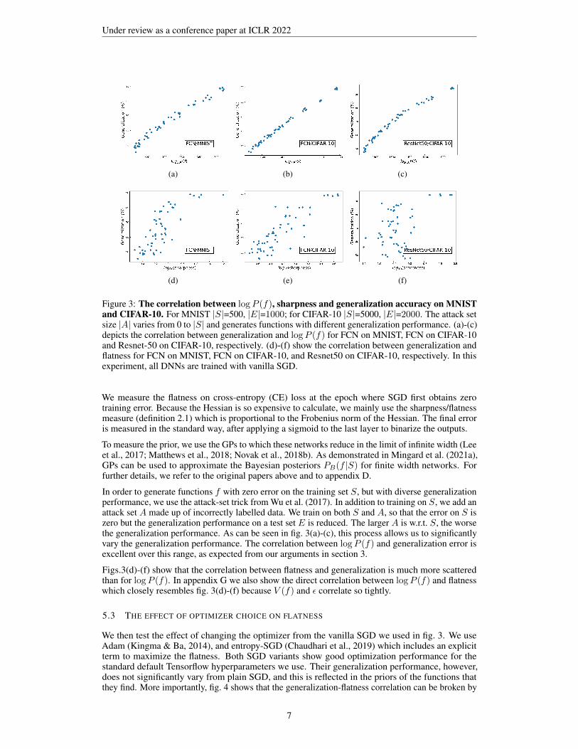
Figure 3: The correlation between logP (f), sharpness and generalization accuracy on MNISTand CIFAR-10. For MNIST |S|=500, |E|=1000; for CIFAR-10 |S|=5000, |E|=2000. The attack setsize |A| varies from 0 to |S| and generates functions with different generalization performance. (a)-(c)depicts the correlation between generalization and logP (f) for FCN on MNIST, FCN on CIFAR-10and Resnet-50 on CIFAR-10, respectively. (d)-(f) show the correlation between generalization andflatness for FCN on MNIST, FCN on CIFAR-10, and Resnet50 on CIFAR-10, respectively. In thisexperiment, all DNNs are trained with vanilla SGD.

We measure the flatness on cross-entropy (CE) loss at the epoch where SGD first obtains zerotraining error. Because the Hessian is so expensive to calculate, we mainly use the sharpness/flatnessmeasure (definition 2.1) which is proportional to the Frobenius norm of the Hessian. The final erroris measured in the standard way, after applying a sigmoid to the last layer to binarize the outputs.

To measure the prior, we use the GPs to which these networks reduce in the limit of infinite width (Leeet al., 2017; Matthews et al., 2018; Novak et al., 2018b). As demonstrated in Mingard et al. (2021a),GPs can be used to approximate the Bayesian posteriors PB(f |S) for finite width networks. Forfurther details, we refer to the original papers above and to appendix D.

In order to generate functions f with zero error on the training set S, but with diverse generalizationperformance, we use the attack-set trick from Wu et al. (2017). In addition to training on S, we add anattack set A made up of incorrectly labelled data. We train on both S and A, so that the error on S iszero but the generalization performance on a test set E is reduced. The larger A is w.r.t. S, the worsethe generalization performance. As can be seen in fig. 3(a)-(c), this process allows us to significantlyvary the generalization performance. The correlation between logP (f) and generalization error isexcellent over this range, as expected from our arguments in section 3.

Figs.3(d)-(f) show that the correlation between flatness and generalization is much more scatteredthan for logP (f). In appendix G we also show the direct correlation between logP (f) and flatnesswhich closely resembles fig. 3(d)-(f) because V (f) and ε correlate so tightly.

5.3 THE EFFECT OF OPTIMIZER CHOICE ON FLATNESS

We then test the effect of changing the optimizer from the vanilla SGD we used in fig. 3. We useAdam (Kingma & Ba, 2014), and entropy-SGD (Chaudhari et al., 2019) which includes an explicitterm to maximize the flatness. Both SGD variants show good optimization performance for thestandard default Tensorflow hyperparameters we use. Their generalization performance, however,does not significantly vary from plain SGD, and this is reflected in the priors of the functions thatthey find. More importantly, fig. 4 shows that the generalization-flatness correlation can be broken by

7


(a) (b) (c)

(d) (e) (f)

Figure 4: SGD-variants can break the flatness-generalization correlation, but not the logP (f)-generalization correlation. The figures show generalization v.s. logP (f) or flatness for the FCNtrained on (a) and (d) – MNIST with Entropy-SGD; (b) and (e) – MNIST with Adam; (c) and (f) –CIFAR-10 with Adam. for the same S and E as in fig. 3. Note that the correlation with the prior isvirtually identical to vanilla SGD, but that the correlation with flatness measures changes significantly.

using these optimizers, whereas the logP (f)-generalization correlation remains intact. A similarbreakdown of the correlation persists upon overtraining and can also be seen for flatness measuresthat use Hessian eigenvalues (fig. S16 to fig. S21).

Changing optimizers or changing hyperparameters can, of course, alter the generalization perfor-mance by small amounts, which may be critically important in practical applications. Nevertheless,as demonstrated in Mingard et al. (2021a), the overall effect of hyperparameter or optimizer changesis usually quite small on these scales. The large differences in flatness generated simply by changingthe optimizer suggests that flatness measures may not always reliably capture the effects of hyperpa-rameter or optimizer changes. Note that we find less deterioration when comparing SGD to Adam forResnet50 on CIFAR-10, (fig. S22). The exact nature of these effects remains subtle.

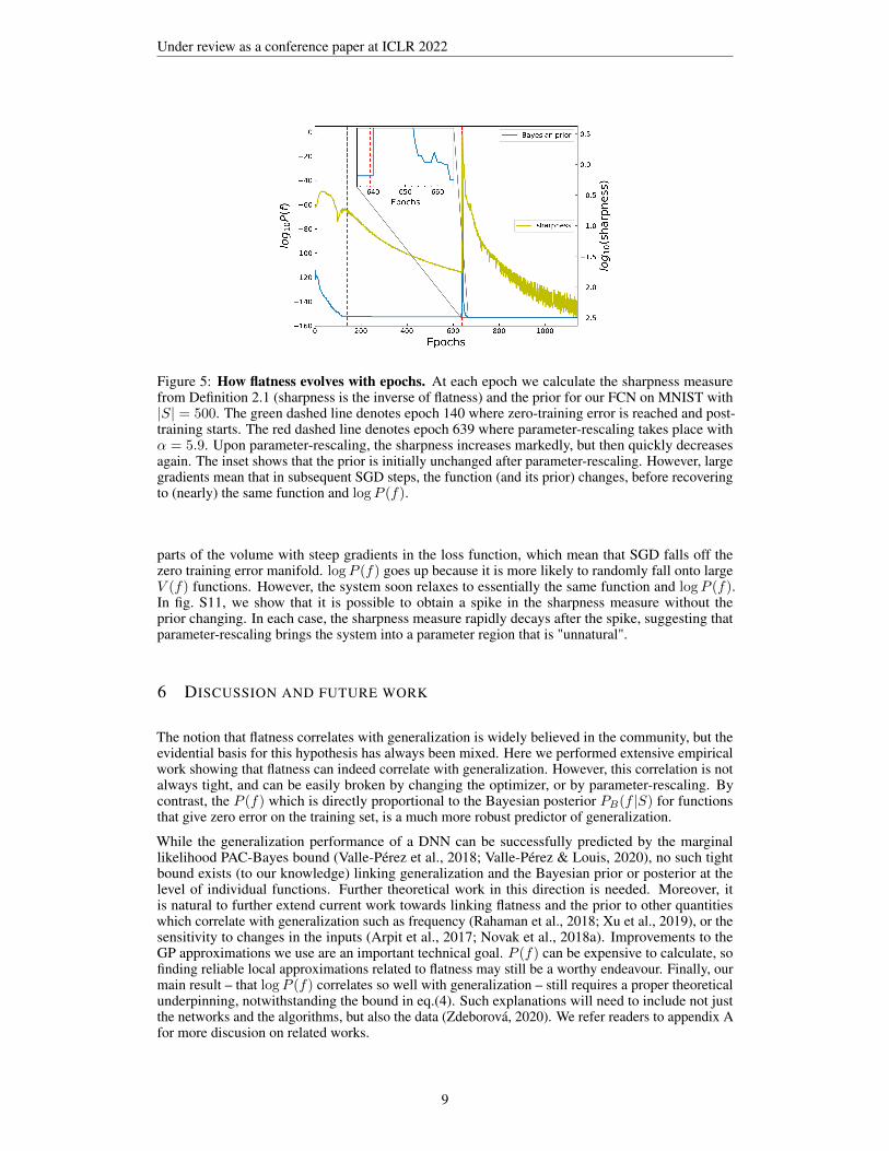
5.4 TEMPORAL BEHAVIOR OF SHARPNESS AND logP (f)

In the experiments above, the flatness and logP (f) metrics are calculated at the epoch where thesystem first reaches 100% training accuracy. In fig. 5, we measure the prior and the flatness for eachepoch for our FCN, trained on MNIST (with no attack set). Zero training error is reached at epoch140, and we overtrain for a further 1000 epochs. From initialization, both the sharpness measure fromDefinition 2.1, and logP (f) reduce until zero-training error is reached. Subsequently, logP (f) staysconstant, but the CE loss continues to decrease, as expected for such classification problems. Thisleads to a reduction in the sharpness measure (greater flatness) even though the function, its prior, andthe training error don’t change. This demonstrates that flatness is a relative concept that depends, forexample, on the duration of training. In figs. S16 and S17 we show for an FCN on MNIST that thequality of flatness-generalization correlations are largely unaffected by overtraining, for both SGDand Adam respectively, even though the absolute values of the sharpness change substantially.

One of the strong critiques of flatness is that re-parameterizations such as the parameter-rescalingtransformation defined in eq. (1) can arbitrarily change local flatness measures (Dinh et al., 2017).Fig. 5 shows that parameter-rescaling indeed leads to a spike in the sharpness measure (a strongreduction in flatness). As demonstrated in the inset, the prior is initially invariant upon parameter-rescaling because f(w) is unchanged. However, parameter-rescaling can drive the system to unusual

8


Figure 5: How flatness evolves with epochs. At each epoch we calculate the sharpness measurefrom Definition 2.1 (sharpness is the inverse of flatness) and the prior for our FCN on MNIST with|S| = 500. The green dashed line denotes epoch 140 where zero-training error is reached and post-training starts. The red dashed line denotes epoch 639 where parameter-rescaling takes place withα = 5.9. Upon parameter-rescaling, the sharpness increases markedly, but then quickly decreasesagain. The inset shows that the prior is initially unchanged after parameter-rescaling. However, largegradients mean that in subsequent SGD steps, the function (and its prior) changes, before recoveringto (nearly) the same function and logP (f).

parts of the volume with steep gradients in the loss function, which mean that SGD falls off thezero training error manifold. logP (f) goes up because it is more likely to randomly fall onto largeV (f) functions. However, the system soon relaxes to essentially the same function and logP (f).In fig. S11, we show that it is possible to obtain a spike in the sharpness measure without theprior changing. In each case, the sharpness measure rapidly decays after the spike, suggesting thatparameter-rescaling brings the system into a parameter region that is "unnatural".

6 DISCUSSION AND FUTURE WORK

The notion that flatness correlates with generalization is widely believed in the community, but theevidential basis for this hypothesis has always been mixed. Here we performed extensive empiricalwork showing that flatness can indeed correlate with generalization. However, this correlation is notalways tight, and can be easily broken by changing the optimizer, or by parameter-rescaling. Bycontrast, the P (f) which is directly proportional to the Bayesian posterior PB(f |S) for functionsthat give zero error on the training set, is a much more robust predictor of generalization.

While the generalization performance of a DNN can be successfully predicted by the marginallikelihood PAC-Bayes bound (Valle-Pérez et al., 2018; Valle-Pérez & Louis, 2020), no such tightbound exists (to our knowledge) linking generalization and the Bayesian prior or posterior at thelevel of individual functions. Further theoretical work in this direction is needed. Moreover, itis natural to further extend current work towards linking flatness and the prior to other quantitieswhich correlate with generalization such as frequency (Rahaman et al., 2018; Xu et al., 2019), or thesensitivity to changes in the inputs (Arpit et al., 2017; Novak et al., 2018a). Improvements to theGP approximations we use are an important technical goal. P (f) can be expensive to calculate, sofinding reliable local approximations related to flatness may still be a worthy endeavour. Finally, ourmain result – that logP (f) correlates so well with generalization – still requires a proper theoreticalunderpinning, notwithstanding the bound in eq.(4). Such explanations will need to include not justthe networks and the algorithms, but also the data (Zdeborová, 2020). We refer readers to appendix Afor more discusion on related works.

9


REFERENCES

Mauricio A Alvarez, Lorenzo Rosasco, and Neil D Lawrence. Kernels for vector-valued functions: A review.arXiv preprint arXiv:1106.6251, 2011.

Devansh Arpit, Stanisław Jastrzebski, Nicolas Ballas, David Krueger, Emmanuel Bengio, Maxinder S Kanwal,Tegan Maharaj, Asja Fischer, Aaron Courville, Yoshua Bengio, et al. A closer look at memorization in deepnetworks. arXiv preprint arXiv:1706.05394, 2017.

Peter L Bartlett, Dylan J Foster, and Matus J Telgarsky. Spectrally-normalized margin bounds for neuralnetworks. In Advances in Neural Information Processing Systems, pp. 6240–6249, 2017.

Leo Breiman. Reflections after refereeing papers for nips. In The Mathematics of Generalization, pp. 11–15.Addison-Wesley, 1995.

Richard H Byrd, Peihuang Lu, Jorge Nocedal, and Ciyou Zhu. A limited memory algorithm for bound constrainedoptimization. SIAM Journal on scientific computing, 16(5):1190–1208, 1995.

Pratik Chaudhari, Anna Choromanska, Stefano Soatto, Yann LeCun, Carlo Baldassi, Christian Borgs, JenniferChayes, Levent Sagun, and Riccardo Zecchina. Entropy-sgd: Biasing gradient descent into wide valleys.Journal of Statistical Mechanics: Theory and Experiment, 2019(12):124018, 2019.

Youngmin Cho and Lawrence Saul. Kernel methods for deep learning. Advances in neural informationprocessing systems, 22:342–350, 2009.

Giacomo De Palma, Bobak Toussi Kiani, and Seth Lloyd. Random deep neural networks are biased towardssimple functions. arXiv preprint arXiv:1812.10156, 2018.

Kamaludin Dingle, Steffen Schaper, and Ard A Louis. The structure of the genotype–phenotype map stronglyconstrains the evolution of non-coding rna. Interface focus, 5(6):20150053, 2015.

Kamaludin Dingle, Chico Q Camargo, and Ard A Louis. Input–output maps are strongly biased towards simpleoutputs. Nature Communications, 9(1):1–7, 2018.

Kamaludin Dingle, Guillermo Valle Pérez, and Ard A Louis. Generic predictions of output probability based oncomplexities of inputs and outputs. Scientific Reports, 10(1):1–9, 2020.

Laurent Dinh, Razvan Pascanu, Samy Bengio, and Yoshua Bengio. Sharp minima can generalize for deep nets.In Proceedings of the 34th International Conference on Machine Learning-Volume 70, pp. 1019–1028. JMLR.org, 2017.

John Duchi, Elad Hazan, and Yoram Singer. Adaptive subgradient methods for online learning and stochasticoptimization. Journal of machine learning research, 12(Jul):2121–2159, 2011.

Gintare Karolina Dziugaite and Daniel M. Roy. Computing nonvacuous generalization bounds for deep(stochastic) neural networks with many more parameters than training data. In Proceedings of the Thirty-ThirdConference on Uncertainty in Artificial Intelligence, UAI 2017, Sydney, Australia, August 11-15, 2017, 2017.URL http://auai.org/uai2017/proceedings/papers/173.pdf.

Adrià Garriga-Alonso, Carl Edward Rasmussen, and Laurence Aitchison. Deep convolutional networksas shallow gaussian processes. In International Conference on Learning Representations, 2019. URLhttps://openreview.net/forum?id=Bklfsi0cKm.

Sebastian Goldt, Marc Mézard, Florent Krzakala, and Lenka Zdeborová. Modelling the influence of datastructure on learning in neural networks. arXiv preprint arXiv:1909.11500, 2019.

Priya Goyal, Piotr Dollár, Ross Girshick, Pieter Noordhuis, Lukasz Wesolowski, Aapo Kyrola, Andrew Tulloch,Yangqing Jia, and Kaiming He. Accurate, large minibatch sgd: Training imagenet in 1 hour. arXiv preprintarXiv:1706.02677, 2017.

Kaiming He, Xiangyu Zhang, Shaoqing Ren, and Jian Sun. Deep residual learning for image recognition. InProceedings of the IEEE conference on computer vision and pattern recognition, pp. 770–778, 2016.

Geoffrey E Hinton and Drew van Camp. Keeping neural networks simple. In International Conference onArtificial Neural Networks, pp. 11–18. Springer, 1993.

Sepp Hochreiter and Jürgen Schmidhuber. Flat minima. Neural Computation, 9(1):1–42, 1997.

10

http://auai.org/uai2017/proceedings/papers/173.pdf

https://openreview.net/forum?id=Bklfsi0cKm


Elad Hoffer, Itay Hubara, and Daniel Soudry. Train longer, generalize better: closing the generalization gap inlarge batch training of neural networks. In Advances in neural information processing systems, pp. 1731–1741,2017.

Sergey Ioffe and Christian Szegedy. Batch normalization: Accelerating deep network training by reducinginternal covariate shift. arXiv preprint arXiv:1502.03167, 2015.

Pavel Izmailov, Dmitrii Podoprikhin, Timur Garipov, Dmitry Vetrov, and Andrew Gordon Wilson. Averagingweights leads to wider optima and better generalization. arXiv preprint arXiv:1803.05407, 2018.

Stanislaw Jastrzebski, Zachary Kenton, Devansh Arpit, Nicolas Ballas, Asja Fischer, Yoshua Bengio, and Amos JStorkey. Finding flatter minima with sgd. In ICLR (Workshop), 2018.

Yiding Jiang, Dilip Krishnan, Hossein Mobahi, and Samy Bengio. Predicting the generalization gap in deepnetworks with margin distributions. arXiv preprint arXiv:1810.00113, 2018.

Yiding Jiang, Behnam Neyshabur, Hossein Mobahi, Dilip Krishnan, and Samy Bengio. Fantastic generalizationmeasures and where to find them. arXiv preprint arXiv:1912.02178, 2019.

Nitish Shirish Keskar, Dheevatsa Mudigere, Jorge Nocedal, Mikhail Smelyanskiy, and Ping Tak Peter Tang. Onlarge-batch training for deep learning: Generalization gap and sharp minima. arXiv preprint arXiv:1609.04836,2016.

Diederik P Kingma and Jimmy Ba. Adam: A method for stochastic optimization. arXiv preprint arXiv:1412.6980,2014.

Alex Krizhevsky, Geoffrey Hinton, et al. Learning multiple layers of features from tiny images. 2009.

Yann LeCun, Léon Bottou, Yoshua Bengio, and Patrick Haffner. Gradient-based learning applied to documentrecognition. Proceedings of the IEEE, 86(11):2278–2324, 1998.

Jaehoon Lee, Yasaman Bahri, Roman Novak, Samuel S Schoenholz, Jeffrey Pennington, and Jascha Sohl-Dickstein. Deep neural networks as gaussian processes. arXiv preprint arXiv:1711.00165, 2017.

L.A. Levin. Laws of information conservation (nongrowth) and aspects of the foundation of probability theory.Problemy Peredachi Informatsii, 10(3):30–35, 1974.

M. Li and P.M.B. Vitanyi. An introduction to Kolmogorov complexity and its applications. Springer-Verlag NewYork Inc, 2008.

Qianli Liao, Brando Miranda, Andrzej Banburski, Jack Hidary, and Tomaso Poggio. A surprising linearrelationship predicts test performance in deep networks. arXiv preprint arXiv:1807.09659, 2018.

Henry W Lin, Max Tegmark, and David Rolnick. Why does deep and cheap learning work so well? Journal ofStatistical Physics, 168(6):1223–1247, 2017.

Yang Liu, Jeremy Bernstein, Markus Meister, and Yisong Yue. Learning by turning: Neural architecture awareoptimisation. arXiv preprint arXiv:2102.07227, 2021.

David JC Mackay. Introduction to gaussian processes. NATO ASI series. Series F: computer and system sciences,pp. 133–165, 1998.

Wesley J Maddox, Gregory Benton, and Andrew Gordon Wilson. Rethinking parameter counting in deep models:Effective dimensionality revisited. arXiv preprint arXiv:2003.02139, 2020.

Susanna Manrubia, José A Cuesta, Jacobo Aguirre, Sebastian E Ahnert, Lee Altenberg, Alejandro V Cano,Pablo Catalán, Ramon Diaz-Uriarte, Santiago F Elena, Juan Antonio García-Martín, et al. From genotypesto organisms: State-of-the-art and perspectives of a cornerstone in evolutionary dynamics. arXiv preprintarXiv:2002.00363, 2020.

Alexander G de G Matthews, Mark Rowland, Jiri Hron, Richard E Turner, and Zoubin Ghahramani. Gaussianprocess behaviour in wide deep neural networks. arXiv preprint arXiv:1804.11271, 2018.

David A McAllester. Some pac-bayesian theorems. In Proceedings of the eleventh annual conference onComputational learning theory, pp. 230–234. ACM, 1998.

Chris Mingard, Joar Skalse, Guillermo Valle-Pérez, David Martínez-Rubio, Vladimir Mikulik, and Ard ALouis. Neural networks are a priori biased towards boolean functions with low entropy. arXiv preprintarXiv:1909.11522, 2019.

11


Chris Mingard, Guillermo Valle-Pérez, Joar Skalse, and Ard A Louis. Is sgd a bayesian sampler? well, almost.Journal of Machine Learning Research, 22(79):1–64, 2021a.

Chris Mingard, Guillermo Valle-Pérez, Joar Skalse, and Ard A Louis. Is sgd a bayesian sampler? well, almost.Journal of Machine Learning Research, 22(79):1–64, 2021b.

Radford M Neal. Priors for infinite networks (tech. rep. no. crg-tr-94-1). University of Toronto, 1994.

Behnam Neyshabur, Srinadh Bhojanapalli, David McAllester, and Nathan Srebro. A pac-bayesian approach tospectrally-normalized margin bounds for neural networks. arXiv preprint arXiv:1707.09564, 2017a.

Behnam Neyshabur, Srinadh Bhojanapalli, David McAllester, and Nati Srebro. Exploring generalization in deeplearning. In Advances in Neural Information Processing Systems, pp. 5949–5958, 2017b.

Roman Novak, Yasaman Bahri, Daniel A Abolafia, Jeffrey Pennington, and Jascha Sohl-Dickstein. Sensitivityand generalization in neural networks: an empirical study. arXiv preprint arXiv:1802.08760, 2018a.

Roman Novak, Lechao Xiao, Jaehoon Lee, Yasaman Bahri, Greg Yang, Jiri Hron, Daniel A Abolafia, JeffreyPennington, and Jascha Sohl-Dickstein. Bayesian deep convolutional networks with many channels aregaussian processes. arXiv preprint arXiv:1810.05148, 2018b.

Henning Petzka, Linara Adilova, Michael Kamp, and Cristian Sminchisescu. A reparameterization-invariantflatness measure for deep neural networks. arXiv preprint arXiv:1912.00058, 2019.

Nasim Rahaman, Aristide Baratin, Devansh Arpit, Felix Draxler, Min Lin, Fred A Hamprecht, Yoshua Bengio,and Aaron Courville. On the spectral bias of neural networks. arXiv preprint arXiv:1806.08734, 2018.

Akshay Rangamani, Nam H Nguyen, Abhishek Kumar, Dzung Phan, Sang H Chin, and Trac D Tran. A scaleinvariant flatness measure for deep network minima. arXiv preprint arXiv:1902.02434, 2019.

Carl Edward Rasmussen. Gaussian processes in machine learning. In Summer School on Machine Learning, pp.63–71. Springer, 2003.

Jorma Rissanen. Modeling by shortest data description. Automatica, 14(5):465–471, 1978.

David E Rumelhart, Geoffrey E Hinton, and Ronald J Williams. Learning representations by back-propagatingerrors. Nature, 323(6088):533–536, 1986.

Levent Sagun, Leon Bottou, and Yann LeCun. Eigenvalues of the hessian in deep learning: Singularity andbeyond. arXiv preprint arXiv:1611.07476, 2016.

Steffen Schaper and Ard A Louis. The arrival of the frequent: how bias in genotype-phenotype maps can steerpopulations to local optima. PloS one, 9(2):e86635, 2014.

Shai Shalev-Shwartz and Shai Ben-David. Understanding machine learning: From theory to algorithms.Cambridge university press, 2014.

Samuel L Smith, Pieter-Jan Kindermans, Chris Ying, and Quoc V Le. Don’t decay the learning rate, increase thebatch size. arXiv preprint arXiv:1711.00489, 2017.

Stefano Spigler, Mario Geiger, and Matthieu Wyart. Asymptotic learning curves of kernel methods: empiricaldata vs teacher-student paradigm. arXiv preprint arXiv:1905.10843, 2019.

Mingyue Tan. Expectation propagation of gaussian process classification and its application to gene expressionanalysis. 01 2008.

Tijmen Tieleman and Geoffrey Hinton. Lecture 6.5-rmsprop: Divide the gradient by a running average of itsrecent magnitude. COURSERA: Neural networks for machine learning, 4(2):26–31, 2012.

Yusuke Tsuzuku, Issei Sato, and Masashi Sugiyama. Normalized flat minima: Exploring scale invariant definitionof flat minima for neural networks using pac-bayesian analysis. arXiv preprint arXiv:1901.04653, 2019.

Guillermo Valle-Pérez and Ard A Louis. Generalization bounds for deep learning. arXiv preprintarXiv:2012.04115, 2020.

Guillermo Valle-Pérez, Chico Q Camargo, and Ard A Louis. Deep learning generalizes because the parameter-function map is biased towards simple functions. arXiv preprint arXiv:1805.08522, 2018.

Mingwei Wei and David J Schwab. How noise affects the hessian spectrum in overparameterized neural networks.arXiv preprint arXiv:1910.00195, 2019.

12


Lei Wu, Zhanxing Zhu, et al. Towards understanding generalization of deep learning: Perspective of losslandscapes. arXiv preprint arXiv:1706.10239, 2017.

Zhi-Qin John Xu, Yaoyu Zhang, Tao Luo, Yanyang Xiao, and Zheng Ma. Frequency principle: Fourier analysissheds light on deep neural networks. arXiv preprint arXiv:1901.06523, 2019.

Greg Yang. Wide feedforward or recurrent neural networks of any architecture are gaussian processes. In H. Wal-lach, H. Larochelle, A. Beygelzimer, F. d'Alché-Buc, E. Fox, and R. Garnett (eds.), Advances in Neural Infor-mation Processing Systems, volume 32. Curran Associates, Inc., 2019. URL https://proceedings.neurips.cc/paper/2019/file/5e69fda38cda2060819766569fd93aa5-Paper.pdf.

Greg Yang and Hadi Salman. A fine-grained spectral perspective on neural networks. arXiv preprintarXiv:1907.10599, 2019.

Zhewei Yao, Amir Gholami, Qi Lei, Kurt Keutzer, and Michael W Mahoney. Hessian-based analysis of largebatch training and robustness to adversaries. In Advances in Neural Information Processing Systems, pp.4949–4959, 2018.

Lenka Zdeborová. Understanding deep learning is also a job for physicists. Nature Physics, 16(6):602–604,2020.

Chiyuan Zhang, Samy Bengio, Moritz Hardt, Benjamin Recht, and Oriol Vinyals. Understanding deep learningrequires rethinking generalization. arXiv preprint arXiv:1611.03530, 2016.

Yao Zhang, Andrew M Saxe, Madhu S Advani, and Alpha A Lee. Energy–entropy competition and theeffectiveness of stochastic gradient descent in machine learning. Molecular Physics, 116(21-22):3214–3223,2018.

13

https://proceedings.neurips.cc/paper/2019/file/5e69fda38cda2060819766569fd93aa5-Paper.pdf

https://proceedings.neurips.cc/paper/2019/file/5e69fda38cda2060819766569fd93aa5-Paper.pdf


A MORE RELATED WORK

A.1 PRELIMINARIES: TWO KINDS OF QUESTIONS GENERALIZATION AND TWO TYPES OFINDUCTIVE BIAS

In this supplementary section we expand on our briefer discussion of related work in the Introduction of themain paper. The question of why and how DNNs generalize in the overparameterized regime has generated avast literature. To organize our discussion, we follow (Mingard et al., 2021a) and first distinguish two kinds ofquestions about generalization in overparameterized DNNs:

1) The question of over-parameterized generalization: Why do DNNs generalize at all in the overparameter-ized regime, where classical learning theory suggests they should heavily overfit.

2) The question of fine-tuned generalization: Given that a DNN already generalizes reasonably well, how candetailed architecture choice, optimizer choice, and hyperparameter tuning further improve generalization?

Question 2) is the main focus of a large tranche of the literature on generalization, and for good reason. In orderto build SOTA DNNs, even a few percent accuracy improvement (taking image classification as an example)is important in practice. Improved generalization performance can be achieved in many ways, includinglocal adjustments of the DNNs structure (e.g. convolutional layers, pooling layers, shortcut connections etc.),hyperparameter tuning (learning rate, batch size etc.), or choosing different optimizers (e.g. vanilla SGD versusentropySGD (Chaudhari et al., 2019) or Adam (Kingma & Ba, 2014). In this paper, however, we are primarilyinterested in question 1). As pointed out, for example famously in Zhang et al. (2016), but also by manyresearchers before that 1, DNNs can be proven to be highly expressive, so that the number of hypotheses that canfit a training data set S, but generalize poorly, is typically many orders of magnitude larger than the numberthat can actually generalize. And yet in practice DNNs do not tend to overfit much, and can generalize well,which implies that DNNs must have some kind of inductive bias (Shalev-Shwartz & Ben-David, 2014) towardhypotheses that generalize well on unseen data.

Following the framework of (Mingard et al., 2021a), we use the language of functions (rather than that ofhypotheses, see also appendix B.) to distinguish two major potential types of inductive bias.

A) The inductive bias upon upon random sampling of parameters over a parameter distribution Pw(w).In other words, given a DNN architecture, loss function etc. and a measure over parameters Pw(w) (which canbe taken to be the initial parameter distribution for an optimizer, but is more general), this bias occurs whencertain types of functions more likely to appear upon random sampling of parameters than others. This inductivebias can be expressed in terms of a prior over functions P (f), or in terms of a posterior PB(f |S) when thefunctions are conditioned, for example, on obtaining zero error on training set S.

B) The inductive bias induced by optimizers during a training procedure. In other words, given an inductivebias upon initialization (from A), does the training procedure induce a further inductive bias on what functionsa DNN expresses? One way of measuring this second form of inductive bias is to calculate the probabilityPopt(f |S) that an DNN trained to zero error on training set S with optimizer opt (typically a variant of SGD)expresses function f , and then compare it to the Bayesian posterior probability PB(f |S) that this functionobtains upon random sampling of parameters (Mingard et al., 2021a). In principle PB(f |S) expresses theinductive bias of type A), so any differences between Popt(f |S) and PB(f |S) could be due to inductive biasesof type B).

These two sources of inductive bias can be relevant to both questions above about generalization. We emphasizethat our taxonomy of two questions about generalization, and two types of inductive bias is just one way ofparsing these issues. We make these first order distinctions to help clarify our discussion of the literature, andare aware that there are other ways of teasing out these distinctions.

A.2 RELATED WORK ON FLATNESS

The concept "flatness" of the loss function of DNNs can be traced back to Hinton & van Camp (1993) andHochreiter & Schmidhuber (1997). Although these authors did not provide a completely formal mathematicaldefinition of flatness, Hochreiter & Schmidhuber (1997) described flat minima as "a large connected regionin parameter space where the loss remains approximately constant", which requires lower precision to specifythan sharp minima. They linked this idea to the minimum description length (MDL) principle (Rissanen, 1978),which says that the best performing model is the one with shortest description length, to argue that flatter minimashould generalize better than sharp minima. More generally, flatness can be interpreted as a complexity controlof the hypotheses class introduced by algorithmic choices.

1For example, Leo Breiman, included the question of overparameterised generalization in DNN back in in1995 as one of the main issues raised by his reflections on 20 years of refereeing for NEURIPS (Breiman, 1995)).

14


The first thing to note is that flatness is a property of the functions that a DNN converges on. In other words, thebasic argument above is that flatter functions will generalize better, which can be relevant to both questions 1)and 2) above.

It is a different question to ask whether a certain way of finding functions (say by optimizing a DNN to zeroerror on a training set) will generate an inductive bias towards flatter functions. In Hochreiter & Schmidhuber(1997), the authors proposed an algorithm to bias towards flatter minima by minimizing the training loss whilemaximizing the log volume of a connected region of the parameter space. This idea is similar to the recentsuggestion of entropy-SGD (Chaudhari et al., 2019), where the authors also introduced an extra regularization tobias the optimizer into wider valleys by maximizing the "local entropy".

In an influential paper, Keskar et al. (2016) reported that the solutions found by SGD with small batch sizesgeneralize better than those found with larger batch sizes, and showed that this behaviour correlated with ameasure of "sharpness" (sensitivity of the training loss to perturbations in the parameters). Sharpness can beviewed as a measure which is the inverse of the flatness introduced by Hinton & van Camp (1993) and Hochreiter& Schmidhuber (1997). This work helped to popularize the notion that SGD itself plays an important role inproviding inductive bias, since differences in generalization performance and in sharpness correlated with batchsize. In follow-on papers others have showed that the correlation with batch size is more complex, as some ofthe improvements can be mimicked by changing learning rates or number of optimization steps for example, see(Hoffer et al., 2017; Goyal et al., 2017; Smith et al., 2017; Neyshabur et al., 2017b). Nevertheless, these changesin generalization as a function of optimizer hyperparameters are important things to understand because they arefundamentally type B) inductive bias. Because the changes in generalization performance in these papers tend tobe relatively small, they mainly impinge on question 2) for fine-tuned generalization. Whether these observedeffects are relevant for question 1) is unclear from this literature.

Another strand of work on flatness has been through the lens of generalization bounds. For example, Neyshaburet al. (2017b) showed that sharpness by itself is not sufficient for ensuring generalization, but can be combined,through PAC-Bayes analysis, with the norm of the weights to obtain an appropriate complexity measure. Theconnection between sharpness and the PAC-Bayes framework was also investigated by Dziugaite & Roy (2017),who numerically optimized the overall PAC-Bayes generalization bound over a series of multivariate Gaussiandistributions (different choices of perturbations and priors) which describe the KL-divergence term appearingin the second term in the combined generalization bound by Neyshabur et al. (2017b). For more discussion ofthis literature on bounds and flatness, see also the recent review (Valle-Pérez & Louis, 2020). Rahaman et al.(2018) also draw a connection to flatness through the lens of Fourier analysis, showing that DNNs typically learnlow frequency components faster than high frequency components. This frequency argument is related to theinput-output sensitivity picture, which is systematically investigated in Novak et al. (2018a).

There is also another wide-spread belief that SGD trained DNNs are implicitly biased towards having smallparameters norms or large margin, intuitively inspired by classical ridge regression and SVMs. Bartlett et al.(2017) presented a margin-based generalization bound that depends on spectral and L2,1 norm of the layer-wiseweight matrices of DNNs. Neyshabur et al. (2017a) later proved a similar spectral-normalized margin boundusing PAC-Bayesian approach rather than the complex covering number argument used in Bartlett et al. (2017).Liao et al. (2018) further strengthen the theoretical arguments that an appropriate measure of complexity forDNNs should be based on a product norm by showing the linear relationship between training/testing CE loss ofnormalized networks. Jiang et al. (2018) also empirically studied the role of margin bounds.

In a recent important large-scale empirical work on different complexity measures by Jiang et al. (2019),40 different complexity measures are tested when varying 7 different hyperparameter types over two imageclassification datasets. They do not introduce random labels so that data complexity is not thoroughly investigated.Among these measures, the authors found that sharpness-based measures outperform their peers, and in particularoutperform norm-based measures. It is worth noting that their definition of "worst case" sharpness is similarto definition 2.1 but normalized by weights, so they are not directly comparable. In fact, their definition ofworst case sharpness in the PAC-Bayes picture is more close to the works by Petzka et al. (2019); Rangamaniet al. (2019); Tsuzuku et al. (2019) which focus on finding scale-invariant flatness measure. Indeed enhancedperformance are reported in these works. However, these measures are only scale-invariant when the scaling islayer-wise. Other methods of re-scaling (e.g. neuron-wise re-scaling) can still change the metrics. Moreover, thescope of Jiang et al. (2019) is concentrated on the practical side (e.g. inductive bias of type B) and does notconsider data complexity, which we believe is a key ingredient to understanding the inductive bias needed toexplain question 1) on generalization.

Finally, in another influential paper, Dinh et al. (2017) showed that many measures of flatness, including thesharpness used in Keskar et al. (2016), can be made to vary arbitrarily by re-scale parameters while keeping thefunction unchanged. This work has called into question the use of local flatness measures as reliable guides togeneralization, and stimulated a lot of follow on studies, including the present paper where we explicitly studyhow parameter-rescaling affects measures of flatness as a function of epochs.

15


A.3 RELATED WORK ON THE INFINITE-WIDTH LIMIT

A series of important recent extensions of the seminal proof in Neal (1994) - that a single-layer DNN withrandom iid weights is equivalent to a GP (Mackay, 1998) in the infinite-width limit - to multiple layers andarchitectures (NNGPs) have recently appeared (Lee et al., 2017; Matthews et al., 2018; Novak et al., 2018b;Garriga-Alonso et al., 2019; Yang, 2019). These studies on NNGPs have used this correspondence to effectivelyperform a very good approximation to exact Bayesian inference in DNNs. When they have compared NNGPs toSGD-trained DNNs the generalization performances have generally shown a remarkably close agreement. Thesefacts require rethinking the role SGD plays in question 1) about generalization, given that NNGPs can alreadygeneralize remarkably well without SGD at all.

A.4 RELATIONSHIP TO PREVIOUS PAPERS USING THE FUNCTION PICTURE

The work in this paper builds on a series of recent papers that have explored the function based picture in randomneural networks. We briefly review these works to clarify their connection to the current paper.

Firstly, in Valle-Pérez et al. (2018), the authors demonstrated empirically that upon random sampling ofparameters, DNNs are highly biased towards functions with low complexity. This behaviour does not dependvery much on Pw(w) for a range of initial distributions typically used in the literature. Note that this behaviourdoes start to deviate from what was found in (Valle-Pérez et al., 2018), when the system enters a chaotic phase,which can be reached with for tanh or erf non-linearities and for Pw(w) with a relatively large variance (Yang& Salman, 2019). They show more specifically that the bias towards simple functions is consistent with the"simplicity bias" from Dingle et al. (2018; 2020), which was inspired by the coding theorem from AIT (Li &Vitanyi, 2008), first derived by Levin (1974) . The idea of simplicity bias in DNNs states that if the parameter-function map is sufficiently biased, then the probability of the DNN producing a function f on input data dropsexponentially with increasing Kolmogorov complexity K(f) of the function f . In other words, high P (f)functions have low K(f), and high K(f) functions have low P (f). A key insight from (Dingle et al., 2018;2020) is that K(f) can be approximated by an appropriate measure K(f) and still be used to make predictionson P (f), even if the true K(f) is formally incomputable. Recently Mingard et al. (2019) and De Palma et al.(2018) gave two separate non-AIT based theoretical justifications for the existence of simplicity bias in DNNs. Inother words, this line of work suggests that DNNs have an intrinsic bias towards simple functions upon randomsampling of parameters, and in our taxonomy, that is bias of type A).

If simplicity bias in DNNs matches "natural" data distributions, then, at least upon random sampling ofparameters, this should help facilitate good generalization. Indeed, it has been shown that data such as MNISTor CIFAR-10 is relatively simple (Lin et al., 2017; Goldt et al., 2019; Spigler et al., 2019), suggesting that aninductive bias toward simplicity will assist with good generalization.

A second paper upon which the current one builds is (Mingard et al., 2021a), where extensive empirical test (fora range of architectures (FCN, CNN, LSTM), datasets (MNIST, Fashion-MNIST, CIFAR-10, ionosphere, IMDbmoviereview dataset), and SGD variants (vanilla SGD, Adam, Adagrad, RMSprop, Adadelta), as well as fordifferent batch sizes and learning rates) were done of the hypothesis that:

Popt(f |S) ≈ PB(f |S). (5)

Here Popt(f |S) is the probability that an optimizer (SGD or one of its variants) converges upon a function fafter training to zero training error on a training set S. By training over many different parameter initializations,Popt(f |S) can be calculated. Similarly, the Bayesian posterior probability PB(f |S) is defined as the probabilitythat upon random sampling of parameters, a DNN expresses function f , conditioned on zero error on S. Thefunctions were, as in the current paper, a restriction to a given training set S and test set E. Since the systemsalways had zero error on the training set, functions could be compared by what they produced on the test set (forexample, the set of labels on the images for image classification). It was found that the hypothesis (A.4) heldremarkably well to first order, for a wide range of systems. At first sight this similarity is surprising, given thatthe procedures to generate Popt(f |S) (training with an optimizer such as SGD) is completely different fromthose for PB(f |S) (where GP techniques and direct sampling were used), which knows nothing of optimizersat all. The fact that these two probabilities are so similar suggests that any inductive bias of type B), whichwould be a bias beyond what is already present in PB(f |S), is relatively small. While this conclusion doesnot imply that there are no induced biases of type B), and clearly there are since hyperparameter tuning affectsfine-tuned generalization, it does suggest that the main source of inductive bias needed to explain 1), the questionof why DNNs generalize in the first place, is found in the inductive biases of type A), which are already therein PB(f |S). In (Mingard et al., 2021a), the authors propose that, for highly biased priors P (f), that SGDis dominated by the large differences in basin size for the different functions f , and so finds functions withprobabilities dominated by the initial distribution. A similar effect was seen in evolutionary systems (Schaper &Louis, 2014; Dingle et al., 2015) where it was called the arrival of the frequent.

16


In addition, in (Mingard et al., 2021a), the authors observed for one system that − log(PB(f |S)) scaled linearlywith the generalization error on E for a wide range of errors. This preliminary result provided inspiration for thecurrent paper where we directly study the correlation between the prior P (f) and the generalization error.

The third main function based paper that we build upon is (Valle-Pérez & Louis, 2020) which provides acomprehensive analysis of generalization bounds. In particular, it studies in some detail the Marginal LikelihoodPAC-Bayes bound, first presented in Valle-Pérez et al. (2018), which is predicts a direct link between thegeneralization error and the log of the marginal likelihood P (S). P (S) can be interpreted as the total priorprobability that a function is found with zero error on the training set S, upon random sampling of parameters ofthe DNN. The performance of the bound was tested for challenges such as varying amounts of data complexity,different kinds of architectures, and different amounts of training data (learning curves). For each challenge itworks remarkably well, and to our knowledge no other bound has been tested this comprehensively. Again, thegood performance of this bound, which is agnostic about optimizers, suggest that a large part of the answer toquestion 1) can be found in the inductive bias of type A), e.g. that found upon initialization. The bound is notaccurate enough to explain smaller effects relevant for fine-tuning generalization, which can originate from othersources such as a difference in optimizer hyperparameters. These conclusions are consistent with the differentapproach in this paper, where we use the prior P (f) (which knows nothing about SGD) and show that it alsocorrelates with predicted test error for DNNS trained with SGD and its variants. We do propose a simpler boundthat is consistent with the observed scaling, but more work is needed to get anywhere near the rigour found in(Valle-Pérez & Louis, 2020) for the full marginal likelihood bound.

Finally, we note that in all three of these papers, GPs are used to calculate marginal likelihoods, posteriors, andpriors. Technical details of how to use GPs can be found clearly explained there.

The current paper builds on this body of work and uses some of the techniques described therein, but it is distinct.Firstly, our measurements on flatness are new, and our claim that the prior P (f) correlates with generalization,while indirectly present in (Mingard et al., 2021a) was not developed there at all as that paper focuses on theposterior PB(f |S), and did not use the attack set trick to vary functions that are consistent with S, and so istackling a different question (namely how much extra inductive bias comes from using SGD over the inductivebias already present in the Bayesian posterior). The attack set trick means that P (S) does not change, whileclearly the generalization error (or expected test error) does change, so the marginal likelihood bound is notpredictive here.

B PARAMETER-FUNCTION MAP AND NEUTRAL SPACE

The link between the parameters of a DNN and the function it expresses is formally described by the parameter-function map:Definition B.1 (Parameter-function map). Consider the model defined in definition 2.2, if the model takesparameters within a set W ⊆ Rn, then the parameter-function mapM is defined as

M : W → Fw 7→ fw.

where fw denotes the function parameterized by w.

The parameter-function map, introduced in (Valle-Pérez et al., 2018), serves as a bridge between a parametersearching algorithm (e.g. SGD) and the behaviour of a DNN in function space. In this context we can also definethe:Definition B.2 (Neutral space). For a model defined in Definition B.1, and a given function f , the neutral spaceNf ⊆W is defined as

Nf := {w ∈W :M(w) = f}.

The nomenclature comes from genotype-phenotype maps in the evolutionary literature (Manrubia et al., 2020),where the space is typically discrete, and a neutral set refers to all genotypes that map to the same phenotype. Inthis context, the Bayesian prior P (f) can be interpreted as the probabilistic volume of the corresponding neutralspace.

C CLARIFICATION ON DEFINITION OF FUNCTIONS AND PRIOR

The discussion of "functions" represented by DNNs can be confusing without careful definition. In fig. S6 welist four different interpretations of "functions" commonly seen in literature which also are directly related to ourwork. These interpretations cover both regression and classification settings. Let X be an arbitrary input domainand Y be the output space. According to different interpretations of the function represented by a DNN, Y willbe different, for the same choice of X and DNN.

17


Figure S6: The diagram of different definitions for functions represented by DNNs.

Definition C.1 (fDNN). Consider a DNN whose input domain is X . Then fDNN belongs to a class of functionsFDNN which define the mapping between X to the pre-activation of the last layer of DNN, which lives in Rd:

fDNN ∈ FDNN : X → Rd

d is the width of the last layer of DNN.

In standard GP terminology, fDNN is also called latent function (Rasmussen, 2003). This is the function we careabout in regression problems.

In the context of supervised learning, we have to make some assumptions about the characteristics of FDNN,as otherwise we would not know how to choose between functions which are all consistent with the trainingsample but might have hugely different generalization ability. This kind of assumptions are called inductivebias. One common approach of describing the inductive bias is to give a prior probability distribution to FDNN,where higher probabilities are given to functions that we consider to be more likely. For DNNs, FDNN is a set offunctions over an (in general) uncountably infinite domain X . There are several approaches to define probabilitydistributions over such sets. GP represent one approach, which generalizes Gaussian distributions to functionspaces. If we ask only for the properties of the functions at a finite number of points, i.e. restriction of FDNN

to C : {c1, . . . , cm} ⊂ X (see definition 2.2), then inference with a GP, reduces to inference with a standardmultidimensional Gaussian distribution. This is an important property of GP called consistency, which helps inmaking computations with GP feasible. As shown in appendix D, we can readily compute with this GP priorover FDNN as long as it is restricted on a finite data set. Later in definition C.4 we will formally define therestricted function fRES.

In classification tasks, we typically get a data sample from X × Y , where without loss of generality Y has theform of Y = {1, . . . , k} where k is the number of classes. For simplicity, we further assume binary classificationwhere Y = {0, 1} Note in the scope of binary classification we have the last layer width of d = 1. To grant theoutputs of the function represented by a DNN a probability interpretation, we need the outputs lie in the interval(0, 1). One way of doing so is to "squash" the outputs of fDNN to (0, 1) by using a final activation, typically alogistic or sigmoid function λ(z) = (1 + exp(−z))−1. Subsequently we have the definition of fACT in fig. S6:Definition C.2 (fACT). Consider the setting and fDNN defined in definition C.1 where d = 1, and a logisticactivation λ(z) = (1 + exp(−z))−1. Then fACT is defined as :

fACT := fDNN ◦ λ : X → (0, 1)

where ◦ denotes function composition. we also define the space of fACT as

FACT = {fACT for every fDNN ∈ FDNN}

In real life classification datasets, we typically do not have access to the probability of an input classified asone certain label, but the labels instead. When we discuss functions represented by DNNs in classification, we

18


usually mean the coarse-grained version of fACT ∈ FACT, meaning we group all outputs to 1 if the probabilityof predicting the inputs as being label "1" is greater or equal than 0.5, and 0 otherwise. Mathematically, wedefine fLAB as:Definition C.3 (fLAB). Consider the setting and fACT defined in definition C.2 and a threshold function

τ(z) =

{1 if z ≥ 0.5

0 otherwise .

Then we define fLAB and the space FLAB as:

fLAB = fACT ◦ τ : X → {0, 1}FLAB = {fLAB for every fACT ∈ FACT}

The definition C.3 allows us to describe the function represented by a DNN in binary classification as a binarystring consisting of "0" and "1", whose length is equal to the size of input domain set |X |. As explained earlier,in classification we also want to put a prior over FLAB and use this prior as our belief about the task beforeseeing any data.

Finally, as we mentioned above, to make computations tractable, we restrict the domain to a finite set of inputs.We use the definition of restriction in definition 2.2 to formally define the "functions" we mean and practicallyuse in our paper:Definition C.4 (fRES). Consider a DNN whose input domain is X with a last layer width d = 1 . LetC = {c1, . . . , cm} ⊂ X be any finite subset of X with cardinality m ∈ N. The restriction of functionspace F ∈ {FDNN,FLAB} to C is denoted as FC , and is defined as the space of all functions from C to Yrealizable by functions in F . We denote with fRES elements of their corresponding spaces of restricted functions.Specifically, in regression:

fRES ∈ FCDNN : C → Rand in binary classification:

fRES ∈ FCLAB : C → {0, 1}

Note that in definition C.4 we only consider scalar outputs in the regression setting. For multiple-output functions,one approach is to consider d GPs and compute the combined kernel (Alvarez et al., 2011).

In statistical learning theory, the function spaces FDNN and FLAB are also called hypotheses classes, with theirelements called hypotheses (Shalev-Shwartz & Ben-David, 2014). It is important to note that our definitionof prior and its calculation is based on the restriction of the hypotheses class to the concatenation of trainingset and test set S + E. Mathematically, this means the prior of a function P (f) we calculated in the paper isprecisely P (fRES), except for the Boolean system in section 5.1, where the input domain X is discrete and smallenough to enumerate (this can also be thought of as the trivial restriction). As explained above, this restriction isinevitable if we want to compute the prior over FDNN or FLAB. A simple example on MNIST (LeCun et al.,1998) can also help to gain a intuition of the necessity of such restriction, where all inputs would include theset of 28x28 integer matrices whose entries take values from 0-255, which gives 256784 possible inputs. Thisindicates that for real-life data distributions the number of all possible inputs is hyper-astronomically large, ifnot infinite. Nevertheless, In some cases, such as the Boolean system described in Valle-Pérez et al. (2018) andtreated in section 5.1, there is no need for such restriction because it is feasible to enumerate all possible inputs:there are only 7 Boolean units which give 27 = 128 possible data sample. However, even in such cases, thenumber of possible functions is still large (2128 ≈ 1038).

D GP APPROXIMATION OF THE PRIOR

In this section, we sketch out how we calculated the prior of a function P (f) (Valle-Pérez et al., 2018; Mingardet al., 2021a). As in those papers, we use GP, which have been shown to be equivalent to DNNs in the limit ofinfinite layer width (Neal, 1994; Lee et al., 2017; Matthews et al., 2018; Tan, 2008; Rasmussen, 2003). Theseneural network GPs (NNGPs) have been shown to accurately approximate the prior over functions P (f) offinite-width Bayesian DNNs (Valle-Pérez et al., 2018; Matthews et al., 2018; Mingard et al., 2021a).

For the NNGPs, a GP prior is placed on the pre-activations z of the last layer of the neural network (beforea final non-linearity, e.g. softmax, is applied), meaning that for any finite inputs set x = {x1, . . . , xm}, therandom output vector (pre-activations) z = [z (x1) , . . . , z (xm)]T has a Gaussian distribution. Note that inthis paper, the the last layer has a single activation since we only focus on binary classification. This setting iscorresponding to the definition of function restriction is definition C.4, with z ∈ Rm. Without loss of generality,we can assume such a process has a zero mean. The prior probability of the outputs z can be calculated as:

P (z) =1

(2π)m2 Σ

12

exp

(−1

2zTΣ−1z

)(6)

19


Σ is the covariance matrix (often called kernel), whose entries are defined as Σ(xi, xj) ≡ E[z(xi), z(xj)]. Neal(1994) gave the basic form of kernel Σ in single hidden layer case, where Σ depends on the variance of weightsand biases (σw and σb). In DNNs with multiple hidden layers, the kernel for layer l can be calculated recursivelyby induction, assuming the layer l − 1 is a GP (Lee et al., 2017; Matthews et al., 2018). The kernel for fullyconnected ReLU-activated networks has a well known arc-cosine kernel analytical form (Cho & Saul, 2009),which we used in all FCNs in our work.

For ResNet50, the analytical form of GP kernel is intractable. Instead, we use a Monte Carlo empirical kernel(Novak et al., 2018b), and apply one step of the fully connected GP recurrence relation (Lee et al., 2017), takingadvantage of the fact that the last layer of ResNet50 is fully connected. Mathematically, the empirical kernel canbe expressed as:

Σ (xi, xj) :=σ2w

Mn

M∑m=1

n∑c=1

(hL−1wm (xi)

)c

(hL−1wm (xj)

)c

+ σ2b (7)

where(hL−1wm (x)

)c

is the activation of c-th neuron in the last hidden layer (L is the total number of layers) forthe network parameterized by the m-th sampling of parameters wm, M is the number of total Monte Carlosampling, n is the width of the final hidden layer, and σw , σb are the weights and biases variance respectively. Inour experiments, M is set to be 0.1× (|S|+ |E|).

After calculating P (z) with the corresponding kernel, the prior over (coarse-grained) restriction of functionsP (f) can be calculated through likelihood P (f |z), which in our case is just a Heaviside function representinga hard sign nonlinearity. As non-Gaussian likelihood produces an intractable P (f), we used ExpectationPropagation (EP) algorithm for the approximation of P (f) (Rasmussen, 2003). This same EP approximationwas used in Mingard et al. (2021a) where it is discussed further. We represent the function f by the input-outputpairs on the concatenation of training set and test set S + E.

E COMPARING FLATNESS METRICS

Figure S7: The direct correlation between sharpness and spectral norm of Hessian for the 1000 mostfrequently found functions found after SGD runs for a two hidden layer FCN, in the n = 7 Booleansystem (Same system as in fig. 2) .

As mentioned in section 2.2 of the main text, the sharpness metric in definition 2.1 can be directly linked tospectral norm of the Hessian by considering the second order Taylor expansion of L(w) around a critical pointin powers of ζ (Dinh et al., 2017). We empirically confirm this relationship by showing in fig. S7 the directcorrelation between sharpness and spectral norm of Hessian, as well as in fig. S8 the correlation between Hessianspectral norm and prior in Boolean system described in section 5.1.

In addition to the spectral norm, another widely used flatness measure is the product of a subset of the positiveHessian eigenvalues, typically say the product of the top-50 largest eigenvalues (Wu et al., 2017; Zhang et al.,2018). We measured the correlation of these Hessian-based flatness metrics with sharpness as well as withgeneralization for the FCN/MNIST system in fig. S9. Since they correlate well with the sharpness, these flatnessmeasures show very similar correlations with generalization as sharpness does in fig. 3 and fig. 4. In other words,the Hessian-based flatness metrics also capture the loose correlation with generalization when the neural networkis trained by SGD and the deterioration of this correlation when we change the optimizer to Adam.

20


Figure S8: The correlation between prior and flatness in Boolean system where the flatness ismeasured by spectral norm of Hessian, for the 1000 most frequently occurring functions found bySGD runs with a two hidden layer FCN. The system is the same n = 7 Boolean system as in fig. 2except that we use a different metric of flatness.

(a) (b) (c) (d)

(e) (f) (g) (h)

Figure S9: Two Hessian-based flatness metrics show analogous behavior to sharpness defined in(definition 2.1). The architecture and dataset are FCN/MNIST, with training set size |S| = 500, andtest set size |E| = 1000; which are the same settings as fig. 3 (d) and fig. 4 (e). Optimizer: SGD (a)- (b): The correlation between Hessian-based flatness metrics and generalization. (c) - (d): Sharpnessand Hessian-based flatness metrics correlate well with one another. Optimizer: Adam (e) - (f): Thecorrelation between Hessian-based flatness metrics and generalization breaks down, just as it does forsharpness in fig. 4. (g) - (h): Sharpness and Hessian-based flatness metrics correlate well with oneanother, even though they don’t correlate well with generalization.

Another detail worth noting is that Keskar et al. (2016) used the L-BFGS-B algorithm (Byrd et al., 1995) toperform the maximization of L(w) in Cζ , which is the box boundary around the minimum of interest:

Cζ = {∆w ∈ Rn : −ζ (|wi|+ 1) ≤ ∆wi ≤ ζ (|wi|+ 1) ∀i ∈ {1, 2, · · · , n}} (8)

However, as a quasi-Newton method, L-BFGS-B is not scalable when there are tens of millions of parameters inmodern DNNs. To make Keskar-sharpness applicable for large DNNs (e.g. ResNet50), we use vanilla SGDfor the maximization instead. The hyperparameters for the sharpness calculation are listed in table 1. Notethat the entries batch size, learning rate and number of epochs all refer to the SGD optimizer which does themaximization in the sharpness calculation process. The number of epochs is chosen such that the max value of

21


Table 1: Hyperparameters for sharpness calculation

DATA SET ARCHITECTURE BOX SIZE (ζ) BATCH SIZE LEARNING RATE NUMBER OF EPOCHS

BOOLEAN FCN 10−4 16 10−3 10MNIST FCN 10−4 32 10−3 100CIFAR10 FCN 10−5 128 5× 10−5 100CIFAR10 RESNET50 10−5 128 100 100

loss function found at each maximization step converges. An example of the convergence of sharpness is shownin fig. S10. As a check, we also compared our SGD-sharpness with the original L-BFGS-B-sharpness, findingsimilar results.

Figure S10: The max value of loss function L(w) at each iteration in the process of maximization,when calculating the sharpness using SGD instead of L-BFGS-B. The plot shows the max loss valuefound by SGD in the box limit Cζ will converge after given number of epochs. For this plot thehyperparameters are listed in the second line of table 1 (MNIST).

F IMPLEMENTING PARAMETER RE-SCALING

In this section we describe in detail how we implement the alpha scaling in DNNs first proposed by Dinh et al.(2017). The widely used rectified linear activation (ReLU) function

φrect(x) = max(x, 0)

exhibits the so-called "non-negative homogeneity" property:

∀(z, α) ∈ R× R+, φrect(zα) = αφrect(z)

The action of a L-layered deep feed-forward neural network can be written as:

y = φrect (φrect (. . . φrect (x ·W1 + b1) . . .) ·WL−1 + bL−1) ·WL + bL

in which

• x is the input vector

• WL is the weight matrix of the L-th layer

• bL is the bias vector of the L-th layer

To simplify notation, we have not included the final activation function, which may take any form (softmax orsigmoid etc.) without modification of the proceeding arguments. Generalizing the original arguments from Dinhet al. (2017) slightly to include bias terms, we exploit the non-negative homogeneity of the ReLU function tofind that a so-called "α-scaling" of one of the layers will not change its behaviour. Explicitly applying this to thei-th layer yields:

(φrect (x · αWi + αbi)) ·1

αWi+1 = (φrect (x ·Wi + bi)) ·Wi+1 (9)

22


Figure S11: The effect of alpha scaling on prior and sharpness. At each epoch we calculate thesharpness and the prior for our FCN on MNIST system with |S| = 500. The green dashed linedenotes where zero-training error is reached and post-training starts. The red dashed line denotes theepoch where α-scaling takes place with α = 5.0. Here the value of α is not big enough to "knock" theoptimizer out of the neutral space, upon alpha scaling, in contrast to fig. 5. As expected, we observeno change in prior upon alpha scaling (note that prior can change on overtraining if a slightly differentfunction is found by SGD). The sharpness shows a larger peak upon alpha-scaling, as expected. Seeappendix H.

Clearly, the transformation described by (Wi, bi,Wi+1)→(αWi, αbi,

1αWi+1

)will lead to an observationally

equivalent network (that is, a network whose output is identical for any given input, even if the weight and biasterms differ).

Since the α scaling transformation does not change the function, it does not change the prior of the function.However, for large enough α, as shown for example in fig. 5, we see that SGD can be "knocked" out of thecurrent neutral space because of the large gradients that are induced by the α scaling. This typically leads tothe prior suddenly surging up, because the random nature of the perturbation means that the system is morelikely to land on large volume functions. However, we always observe that the prior then drops back down quitequickly as SGD reaches zero training error again. On the other hand, as shown in fig. S11, when the value of αis smaller it does not knock SGD out of the neutral space, and so the prior does not change at all. Nevertheless,the sharpness still exhibits a strong spike due to the the alpha scaling.

Although not in the scope of this work, it is worth noting that the alpha scaling process in Convolutional NeuralNetworks (CNNs) with batch normalization (Ioffe & Szegedy, 2015) layer(s) is somewhat different. Becausea batch normalization layer will eliminate all affine transformations applied on its inputs, one can arbitrarilyalpha scale the layers before a batch normalization layer without needing to of compensate in following layer,provided the scaling is linear.

G FLATNESS AND PRIOR CORRELATION

In the main text, we showed the correlation of the Bayesian prior and of sharpness with generalization in fig. 3and fig. 4. Here, in fig. S12, we show the direct correlation of the prior and sharpness. As expected from thefigures in the main text, sharpness correlates with prior roughly as it does with generalization - i.e. reasonablyfor vanilla SGD but badly for entropy-SGD (Chaudhari et al., 2019) or Adam (Kingma & Ba, 2014). We notethat, as shown in fig. S9, sharpness also correlates relatively well with the spectral norm of the Hessian and logproduct of its 50 largest eigenvalues for all the optimizers. So the correlation of flatness with prior/generalizationdoes not depend much on which particular flatness measure is used.

Overall, it is perhaps unsurprising that a local measure such as flatness varies in how well it approximates theglobal prior. What is unexpected (at least to us) is that Adam and Entropy-SGD break the correlation for thisdata set. In appendix J.2, we show that this correlation also breaks down for other more complex optimizers,but, interestingly, not for full-batch SGD. Further empirical and theoretical work is needed to understand thisphenomenon. For example, is the optimizer dependence of the correlation between flatness and prior a generalproperty of the optimizer, or is it specific to certain architectures and datasets? One hint that these resultsmay have complex dependencies on architecture and dataset comes from our observation that for ResNet50 on

23


Cifar10, we see less difference between SGD and Adam than we see for the FCN on MNIST. More work isneeded here.

(a) (b) (c)

(d) (e) (f)

Figure S12: The direct correlation between prior P (f) and sharpness over different datasets andoptimizers. The correlation between prior and sharpness closely resembles the correlation betweensharpness and generalization, mainly because prior and generalization are very closely correlated, asseen in our experiments (fig. 3, fig. 4).

H TEMPORAL BEHAVIOR OF SHARPNESS

When using sharpness in definition 2.1 as the metric of flatness, there are several caveats. First is the hyper-parameters (see table 1): the value of sharpness is only meaningful under specified hyperparameters, and indifferent experiments the sharpnesses are only comparable when the hyperparameters are the same. This renderssharpness less convenient to use (but still much more efficient than Hessian calculation). Second is the timeevolving behavior of sharpness: For the classification problems we study, and for CE loss, it can continue tochange even when the function (and hence generalization) is unchanged.

Before reaching zero training error, gradients can be large, and the behavior of sharpness (definition 2.1) can beunstable under changes of box size ζ. This effect is likely the cause of some unusual fluctuations in the sharpnessthat can be observed in fig. 5 and fig. S11 around epoch 100. In fig. S13 we show that this artefact disappears forlarger ζ. Similarly, when the gradients are big (typical in training), sharpness may no longer link to spectralnorm of Hessian very well.

In fig. S14, we first train the FCN to zero error, then "alpha scale" after 500 epochs, and then keep post-trainingfor another 5000 epochs, much longer than in fig. 5. The behaviour of sharpness and prior upon "alpha scaling"(not surprisingly) follows our discussion in section 5.4. What is interesting to see here is that after enoughovertraining, the effect of the alpha scaling spike appears to disappear, and the overall curve looks like acontinuation of the curve prior to alpha scaling. What this suggests is that alpha-scaling brings the system to anarea of parameter space that is somehow "unnatural". Again, this is a topic that deserves further investigation inthe future.

Finally, we show the temporal behavior of a Hessian-based flatness measure in fig. S15. Because of the largememory cost when calculating the Hessian, we use a smaller FCN on MNIST, with the first hidden layer having10 units. We find that the Hessian based flatness exhibit similar temporal behavior to sharpness.

24


(a) (b) (c)

Figure S13: Different temporal behavior of sharpness, prior and accuracy when using differentbox size ζ. The dataset is MNIST with |S| = 500 and |E| = 100. The architecture is FCN. SGDoptimizer is used. Scaling parameter α = 5.0. Green and red dashed line denote reaching zerotraining error and alpha scaling, respectively. (a) ζ = 10−3, (b) ζ = 10−4, (c) ζ = 10−5. While thereare quantitative differences between the values of ζ used, qualitatively we observe similar behaviour.

Figure S14: The temporal behavior of sharpness and prior after 5000 epochs of reaching zero trainingerror. The dataset is MNIST with |S| = 500 and |E| = 100. The architecture is FCN. SGD optimizeris used. The magnitude of scaling α = 6.0.

I THE CORRELATION BETWEEN GENERALIZATION, PRIOR, AND SHARPNESSUPON OVERTRAINING

As shown in fig. 5 of the main text, and further discussed in appendix H, flatness measures keep decreasing uponovertraining even when the function itself does not change. In this section, we revisit the correlation betweenprior, flatness and generalization at different numbers of overtraining epochs, i.e. after reaching zero trainingerror.As can be seen in fig. S16 to fig. S21, overtraining does not meaningfully affect the correlation betweensharpness, prior, and generalization we observed at the epoch where zero error is first reached in fig. 3 and fig. 4.When the optimizer is SGD, the flatness, no matter if it is measured by sharpness or Hessian based metrics,correlates well with prior and (hence) generalization across difference overtraining epochs; whereas when usingAdam, the poor correlation also persist in overtraining.

J FURTHER EXPERIMENTS

J.1 RESNET50 TRAINED WITH ADAM

When training ResNet50 on CIFAR-10, we use training set size |S| = 5000, attack set size |A| = 5000, testset size |E| = 2000. In each experiment, we mix the whole training set with different size of subset of attackset. The size of |A| ranges as (0, 500, 1000, 1500, ..., 5000). For each subset of attack set we sample 5 times.When training ResNet50 with Adam, we empirically found it is hard to train the neural net to zero training errorwith attack set size |A| > 2500. So we only show the results for those functions found with |A| ≤ 2500. In

25


Figure S15: The temporal behavior of one Hessian based flatness metric. The dataset is MNIST with|S| = 500 and |E| = 100. The architecture is a smaller FCN (784-10-40-1), the optimizer is SGD.The green dashed line denotes the epoch where the system reaches zero training error. No alphascaling is applied here. The Hessian based flatness metric shows similar temporal behaviour to thesharpness measure.

fig. S22 we show the results of correlation between sharpness and prior with generalization with limited data.The prior, as usual, correlates tightly with generalization, while the flatness-generalization correlation is muchmore scattered, although it is slightly better than the correlation seen for the FCN on MNIST, and closer to thebehaviour we observed for SGD in the main text.

J.2 MORE SGD-VARIANT OPTIMIZERS

In fig. S23 we provide further empirical results for the impact of choice of optimizer on the sharpness-generalization correlation by studying three common used SGD variants: Adagrad (Duchi et al., 2011),Momentum (Rumelhart et al., 1986) (momentum=0.9) and RMSProp (Tieleman & Hinton, 2012), as wellas full batch gradient descent. Interestingly, full batch gradient descent (or simply gradient descent) showsbehaviour that is quite similar to vanilla SGD. By contrast, for the other three optimizers, the correlation betweensharpness and generalization breaks down, whereas the correlation between prior and generalization remainsintact, much as was observed in the main text for Adam and Entropy-SGD. .

J.3 LARGER TRAINING SET

In order to rule out any potential training size effect on our main argument of the flatness, prior and generalizationrelationship, we further performed the experiments on MNIST with 10k training examples. Larger training setsare hard because of the GP-EP calculation of the prior scales badly with size. The results are shown in fig. S24.It is clear that the correlations between sharpness, prior and generalization follow the same pattern as we see infig. 3, in which there are only |S| = 500, |E| = 1000 images. If anything, the correlation with prior is tighter.

26


Figure S16: The correlation between sharpness, prior and generalization upon overtraining. Thedataset is MNIST (|S| = 500, |E| = 1000), the optimizer is SGD. For the range of (100-500)overtraining epoch tested here, the overall values of sharpness drop with overtraining. By contrast,the priors remain largely the same. For each quantity, the correlations remain remarkably similar withovertraining.

27


Figure S17: The correlation between sharpness, prior and generalization when over-trained (keeptraining after reaching zero training error). The dataset is MNIST (|S| = 500, |E| = 1000), theoptimizer is Adam. The correlations are similar across different overtraining epochs.

28


Figure S18: The correlation between Hessian spectral norm, prior and generalization when over-trained (keep training after reaching zero training error). The dataset is MNIST (|S| = 500, |E| =1000), the optimizer is SGD. The correlations are similar across different overtraining epochs.

29


Figure S19: The correlation between Hessian based flatness (product of the top 50 largest Hessianeigenvalues), prior and generalization when over-trained (keep training after reaching zero trainingerror). The dataset is MNIST (|S| = 500, |E| = 1000), the optimizer is SGD. The correlations aresimilar across different overtraining epochs.

30


Figure S20: The correlation between Hessian spectral norm, prior and generalization when over-trained (keep training after reaching zero training error). The dataset is MNIST (|S| = 500, |E| =1000), the optimizer is Adam. The correlations are similar across different overtraining epochs.

31


Figure S21: The correlation between Hessian based flatness (product of the top 50 largest Hessianeigenvalues), prior and generalization when over-trained (keep training after reaching zero trainingerror). The dataset is MNIST (|S| = 500, |E| = 1000), the optimizer is Adam. The correlations aresimilar across different overtraining epochs.

32


(a) (b)

Figure S22: The correlation between generalization and (a) sharpness (b) prior for ResNet50 with|S| = 5000, |E| = 2000, and |A| ranging from 0 to 2500, all on CIFAR-10.

33


Figure S23: More results on the correlation between sharpness, prior and generalization when usingother SGD-variant optimizers. The dataset is MNIST, |S| = 500, |E| = 1000. The architecture isFCN. The optimizers are full-batch gradient descent, Adagrad, Momentum (momentum=0.9) andRMSProp. All correlations are measured upon reaching zero training error.

34


(a) (b) (c)

(d) (e) (f)

Figure S24: The correlation between sharpness, prior and generalization on MNIST with |S| =10000, |E| = 1000. The attack set size ranges from 1000 to 9000. The architecture is FCN. (a)-(c):The FCN is trained with SGD; (d)-(f): The FCN is trained with Adam.

35

LATE WITH GENERALIZATION FOR DEEP NEU - OpenReview

Documents

Transcript of LATE WITH GENERALIZATION FOR DEEP NEU - OpenReview