plants

Article

Machine Learning Undercounts Reproductive Organs onHerbarium Specimens but Accurately Derives Their QuantitativePhenological Status: A Case Study of Streptanthus tortuosus

Natalie L. R. Love 1,2,* , Pierre Bonnet 3 , Hervé Goëau 3 , Alexis Joly 4 and Susan J. Mazer 1

�����������������

Citation: Love, N.L.R.; Bonnet, P.;

Goëau, H.; Joly, A.; Mazer, S.J.

Machine Learning Undercounts

Reproductive Organs on Herbarium

Specimens but Accurately Derives

Their Quantitative Phenological

Status: A Case Study of

Streptanthus tortuosus. Plants 2021, 10,

2471. https://doi.org/10.3390/

plants10112471

Academic Editor: Hazem M. Kalaji

Received: 20 October 2021

Accepted: 12 November 2021

Published: 16 November 2021

Publisher’s Note: MDPI stays neutral

with regard to jurisdictional claims in

published maps and institutional affil-

iations.

Copyright: © 2021 by the authors.

Licensee MDPI, Basel, Switzerland.

This article is an open access article

distributed under the terms and

conditions of the Creative Commons

Attribution (CC BY) license (https://

creativecommons.org/licenses/by/

4.0/).

1 Department of Ecology, Evolution, and Marine Biology, University of California,Santa Barbara, CA 93106, USA; sjmazer@ucsb.edu

2 Biological Sciences Department, California Polytechnic State University, San Luis Obispo, CA 93407, USA3 Botany and Modeling of Plant Architecture and Vegetation (AMAP), French Agricultural Research Centre for

International Development (CIRAD), French National Centre for Scientific Research (CNRS), French NationalInstitute for Agriculture, Food and Environment (INRAE), Research Institute for Development (IRD),University of Montpellier, 34398 Montpellier, France; pierre.bonnet@cirad.fr (P.B.);herve.goeau@cirad.fr (H.G.)

4 ZENITH Team, Laboratory of Informatics, Robotics and Microelectronics-Joint Research Unit,Institut National de Recherche en Informatique et en Automatique (INRIA) Sophia-Antipolis, CEDEX 5,34095 Montpellier, France; alexis.joly@inria.fr

* Correspondence: nlove@ucsb.edu or nllove@calpoly.edu

Abstract: Machine learning (ML) can accelerate the extraction of phenological data from herbariumspecimens; however, no studies have assessed whether ML-derived phenological data can be usedreliably to evaluate ecological patterns. In this study, 709 herbarium specimens representing awidespread annual herb, Streptanthus tortuosus, were scored both manually by human observersand by a mask R-CNN object detection model to (1) evaluate the concordance between ML andmanually-derived phenological data and (2) determine whether ML-derived data can be used toreliably assess phenological patterns. The ML model generally underestimated the number ofreproductive structures present on each specimen; however, when these counts were used to providea quantitative estimate of the phenological stage of plants on a given sheet (i.e., the phenologicalindex or PI), the ML and manually-derived PI’s were highly concordant. Moreover, herbariumspecimen age had no effect on the estimated PI of a given sheet. Finally, including ML-derived PIs aspredictor variables in phenological models produced estimates of the phenological sensitivity of thisspecies to climate, temporal shifts in flowering time, and the rate of phenological progression that areindistinguishable from those produced by models based on data provided by human observers. Thisstudy demonstrates that phenological data extracted using machine learning can be used reliably toestimate the phenological stage of herbarium specimens and to detect phenological patterns.

Keywords: regional convolutional neural network; object detection; deep learning; visual dataclassification; climate change; natural history collections; phenological stage annotation; floweringtime; phenological shift; phenology

1. Introduction

Within and among plant species, the study of phenological traits such as the timing ofbud break or flowering can provide key insights into how species respond to climate [1].Measuring the relationship between phenology and local environmental conditions enablesus to evaluate the sensitivity of phenological events to changes in temperature, precipi-tation, and other climatic parameters as well as to predict future phenological shifts inresponse to projected climate change [2]. Plant phenology mediates complex species in-teractions (e.g., plant–plant, plant–herbivore, plant–pollinator; [3–5]); therefore, climate

Plants 2021, 10, 2471. https://doi.org/10.3390/plants10112471 https://www.mdpi.com/journal/plants

Plants 2021, 10, 2471 2 of 17

change-induced disruptions to plant phenology may have cascading effects on the func-tions and persistence of ecosystems. While previous studies have documented a wide rangeof phenological responses to climate and climate change [6,7], our understanding of theseresponses in many taxa and ecosystems remains incomplete. This gap limits our ability tomake broad scale predictions of the ecosystem-wide impacts from climate change [8,9].

Natural history collections, such as herbarium specimens, provide a long temporalrecord of phenology for hundreds of thousands of taxa globally and offer a data-richresource with which to fill this gap [6]. Moreover, herbarium specimens can be used totrack phenological responses to climate and climate change [10–12]. With large-scale effortsto digitize and image herbarium records, millions of herbarium records are now availablevia large data aggregators, e.g., GBIF (https://www.gbif.org/ (accessed on 1 October2020))and iDigBio (https://www.idigbio.org/ (accessed on 1 October 2020)), to advancephenological research.

The majority of herbarium specimens include the name of the sampled species (al-though the scientific name may not be up to date), the precise date of collection, and atext description of the location at which the specimen was collected, which may include anote indicating whether or not the specimen was collected in flower. A smaller fraction ofherbarium specimens have also been georeferenced to provide the latitude and longitudeof the site of collection (including estimates of the spatial uncertainty of the geographiccoordinates, which may range from 0–25 km). These attributes of specimens, when avail-able, are routinely included in electronic databases provided by the herbaria that archivethe physical specimens. By contrast, electronic records of herbarium specimens rarelyinclude reports of the numbers of flower buds, open flowers, developing ovaries, andfull-sized or mature fruits. Previous work by Love et al. [13], Love and Mazer [14], andMazer et al. [15] found that analyses that include a quantitative estimate of the phenologicalstatus of herbarium specimens—ranging from those bearing only flower buds (i.e., whenthe plant is collected at the beginning of a reproductive cycle) to those bearing only ripefruits (i.e., when the plant is collected at the end of an annual or irregular reproductivecycle)—as a predictor variable in models designed to detect the effect of local climate onflowering date can improve their predictive capacity. In addition, this information can beused to estimate the rate at which a species progresses phenologically from bud throughfruit production [13]. However, scoring specimens to record the numbers of differenttypes of reproductive organs in order to estimate quantitatively their phenological statusrequires substantial human investment. Although citizen scientists can provide valuablecontributions to the scoring process [16], it remains a challenging task that will be difficultto implement at large scales.

Recently, machine learning techniques—specifically, convolutional neural networks(CNN)—have been used to harvest accurate phenological data from imaged herbariumspecimens [17–19], and represents a promising approach for large-scale and automatedphenological data extraction [20]. For example, Lorieul et al. [17] used CNN to distinguishfertile from non-fertile specimens (i.e., coarse-scale or first-order scoring; [21]) of thousandsof species with an accuracy of 96.3% (percent of specimens correctly classified as fertileor non-fertile). Their algorithm was also used for finer-scale (i.e., second-order scoring orscoring the presence/absence of flowers and fruits) scoring and demonstrated an accuracyof 84.3% and 80.5% for flower and fruit detection, respectively.

Machine learning has also been used successfully to detect and count individualreproductive structures on herbarium sheets (i.e., third-order scoring) using instancesegmentation (mask R-CNN or regional CNN; [18,19]). Goëau et al. [19] trained a modelusing only 21 manually-scored herbarium sheets bearing a total of 279 buds, 349 openflowers, 196 developing ovaries, and 212 full-sized fruits that resulted in accurate estimatesof the number of reproductive structures present on a given herbarium sheet (77.9%accuracy); however, the level of accuracy depended on the type of structure being detected(i.e., flowers vs. fruits). While these studies demonstrate that machine learning can beused to automate scoring, no studies have assessed whether machine learning-derived

Plants 2021, 10, 2471 3 of 17

phenological data can be used reliably to evaluate ecological patterns such as estimatingthe phenological sensitivity of flowering date to climate or estimating phenological shiftsin response to contemporary climate change (but see [13] for a preliminary study).

In this study, we use a set of 709 herbarium specimens of Streptanthus tortuosusKellogg (Brassicaceae) that were scored both manually (by human observers) and byusing mask R-CNN to assess the concordance between human- and machine-learning-derived phenological data and to evaluate the use of automated phenological scoring inphenological research. Specifically, we addressed the following questions:

1. Can machine learning be used to obtain counts of reproductive organs on herbariumspecimens that match those recorded by human observers?

2. Do distinct organ types (e.g., flower buds, open flowers, or fruits) differ with respect tothe degree to which machine-learned counts match those recorded by human observers?

3. When counts obtained via machine learning are used to estimate the phenologicalindex (PI)—a quantitative metric of the phenological status of an herbarium specimenthat reflects the proportions of different types of reproductive organs (Love et al.,2019)—does the machine-generated PI match the PI calculated from counts reportedby human observers?

4. Does the year of specimen collection affect counting error or estimation of the phe-nological status? For example, does the fading of floral pigments over time make itmore difficult for machine learning algorithms to distinguish between buds and openflowers as herbarium specimens age?

5. When the phenological status (PI) of specimens generated by machine learning is usedto construct models that provide estimates of the rate of temporal shifts in floweringdate, the sensitivity to climate, and the rate of phenological progression, do theseestimates match those based on data derived from human observers?

Despite the potential for errors in human-derived counts of reproductive structures,in the current study we assume that human-counted values are more correct than machine-learning counted values. We treat human-observed values as the true values against whichwe compare values derived from machine learning to assess its accuracy in extractingphenological data from herbarium specimens.

2. Results2.1. Herbarium Data

Our final testing dataset consisted of 709 georeferenced herbarium specimens that werescored both manually and via the machine-learning model. These specimens’ collectiondates spanned a 112-year period (1902–2013) and the sites of collection were distributedthroughout S. tortuosus’ geographic range (Figure S1). The mean DOY (day of year ofspecimen collection between 1 and 365) among all specimens was day 182 (1 July; SD = 35.2,range: 76–256). The spring mean maximum daily temperature (spring Tmax) and cumulativewinter precipitation experienced at each collection site during the year of specimen collectionranged from 1.4–24.6 ◦C (SD = 4.8 ◦C) and 88–2167 mm (SD = 357.8 mm), respectively.

The 21 herbarium specimens used to train the mask R-CNN model were collectedbetween 1899 and 1983. The number of reproductive organs per sheet depended on the typeof organ, as follows: buds (range: 0–78; SD = 18), flowers (range: 0–70; SD = 18), immaturefruits (range: 0–30; SD = 9), and mature fruits (range: 0–32; SD: 12). The manually-derivedPI of the training set ranged from 1.12 to 3.96 (Table S1).

2.2. Phenological Scoring: Manual vs. Machine Learning

The machine learning model generally under-estimated the number of structuresrelative to manual counts (i.e., human observers) across all categories (buds, flowers,immature fruits, and mature fruits; Figures 1 and 2); however, the degree to which themodel under-estimated counts depended on the type of structure being detected. Maturefruits showed the strongest concordance between predicted (machine learning-derived) vs.manual counts (r = 0.75) while flowers showed the weakest (r = 0.57; Figure 1). The slopes

Plants 2021, 10, 2471 4 of 17

of the linear regressions between predicted vs. manual counts indicated that, on average,the algorithm detected 1 bud for every 6.2 manually-counted buds and 1 mature fruitfor every 3.6 manually counted mature fruits present on each sheet (buds = 0.16 ± 0.007predicted per manually-counted bud, p < 0.0001; mature fruits = 0.28 ± 0.009 predictedper manually-counted mature fruit, p < 0.0001; Table S2). These slope estimates rangedfrom 0.16 ± 0.007 buds to 0.30 ± 0.01 immature fruits predicted per manually-countedstructure (Table S2). The regression R2 for all models ranged from 0.32 (flowers) to 0.56(mature fruits; Table S2). For all organ types, there were fewer counting errors when fewerorgans (or overlapping organs) were present on the sheet (Figures 2 and 3; Table 1).

Despite underestimation across all classes, there was high concordance between ma-chine learning-derived estimates of the PI and those derived from manual counts (r = 0.91;Figure 4). The slope of the linear regression between machine-learning- vs. manually-derived PI values for each record also indicates high concordance (slope = 0.91 ± 0.01,p < 0.0001, R2 = 0.82; Figure 4, Table S2).

Plants 2021, 10, x FOR PEER REVIEW 5 of 19

Figure 1. Bi-variate relationship between the number (#) of organs predicted by the machine-learning model vs. those counted manually by human observers for (A) buds, (B) flowers, (C) immature fruits, and (D) mature fruits. The dashed diagonal line shows a hypothetical 1:1 relationship where the manual and true counts are the same. The solid line denotes the linear regression between predicted and manual counts. Summaries for each regression can be found in Table S2.

Figure 1. Bi-variate relationship between the number (#) of organs predicted by the machine-learningmodel vs. those counted manually by human observers for (A) buds, (B) flowers, (C) immature fruits,and (D) mature fruits. The dashed diagonal line shows a hypothetical 1:1 relationship where themanual and true counts are the same. The solid line denotes the linear regression between predictedand manual counts. Summaries for each regression can be found in Table S2.

Plants 2021, 10, 2471 5 of 17Plants 2021, 10, x FOR PEER REVIEW 6 of 19

Figure 2. Box plots of counting error vs. number of reproductive units present on each herbarium specimen (as estimated manually by human observers) for (A) buds, (B) flowers, (C) immature fruits, and (D) mature fruits. The numbers below each box plot denote the number of herbarium specimens represented in each box plot.

Figure 2. Box plots of counting error vs. number of reproductive units present on each herbariumspecimen (as estimated manually by human observers) for (A) buds, (B) flowers, (C) immature fruits,and (D) mature fruits. The numbers below each box plot denote the number of herbarium specimensrepresented in each box plot.

Table 1. Summary statistics showing the numbers of reproductive structures in each class present oneach sheet as determined by human observers (i.e., manually-derived counts). The mean averageerror (MAE) was calculated and used to evaluate the performance of the machine learning model.The MAE measures the mean absolute error per class of reproductive structure across all sheets.

Reproductive Structure Number per Sheet (Range) Mean ± SD per Sheet MAE

Buds 0–344 27.4 ± 30.6 19.7lFowers 0–227 28.5 ± 26.4 16.6

Immature fruits 0–87 11.0 ± 12.7 6.5Mature fruits 0–131 12.5 ± 19.3 8.3

Plants 2021, 10, 2471 6 of 17Plants 2021, 10, x FOR PEER REVIEW 7 of 19

Figure 3. Examples of manually produced masks used to train the recognition model. In the specimen on the left, several mature fruits overlap, so only the structures in the foreground were annotated in this case, resulting in the exclusion of background structures from the segmentation in that part of the image. The specimen on the right displays examples of predicted masks (buds in red, flowers in purple, immature fruits in orange, mature fruits in blue) on a test specimen. The organs that were not detected (flowers in green rectangles and immature fruit in a yellow rectangle) are either very largely degraded, or partially hidden behind stems or leaf lamina.

Despite underestimation across all classes, there was high concordance between machine learning-derived estimates of the PI and those derived from manual counts (r = 0.91; Figure 4). The slope of the linear regression between machine-learning- vs. manually-derived PI values for each record also indicates high concordance (slope = 0.91 ± 0.01, p < 0.0001, R2 = 0.82; Figure 4, Table S2).

Figure 3. Examples of manually produced masks used to train the recognition model. In the specimen on the left, severalmature fruits overlap, so only the structures in the foreground were annotated in this case, resulting in the exclusion ofbackground structures from the segmentation in that part of the image. The specimen on the right displays examples ofpredicted masks (buds in red, flowers in purple, immature fruits in orange, mature fruits in blue) on a test specimen. Theorgans that were not detected (flowers in green rectangles and immature fruit in a yellow rectangle) are either very largelydegraded, or partially hidden behind stems or leaf lamina.

Plants 2021, 10, x FOR PEER REVIEW 8 of 19

Figure 4. Bivariate plot showing the relationship between the phenological index (PI) as estimated using predicted counts vs. manual counts (counted by human observers). The solid gray line denotes the linear regression between the two estimates of PI. The dashed black line shows a hypothetical 1:1 relationship where the two estimates result in the same PI value. Summaries for the regression can be found in Table S2.

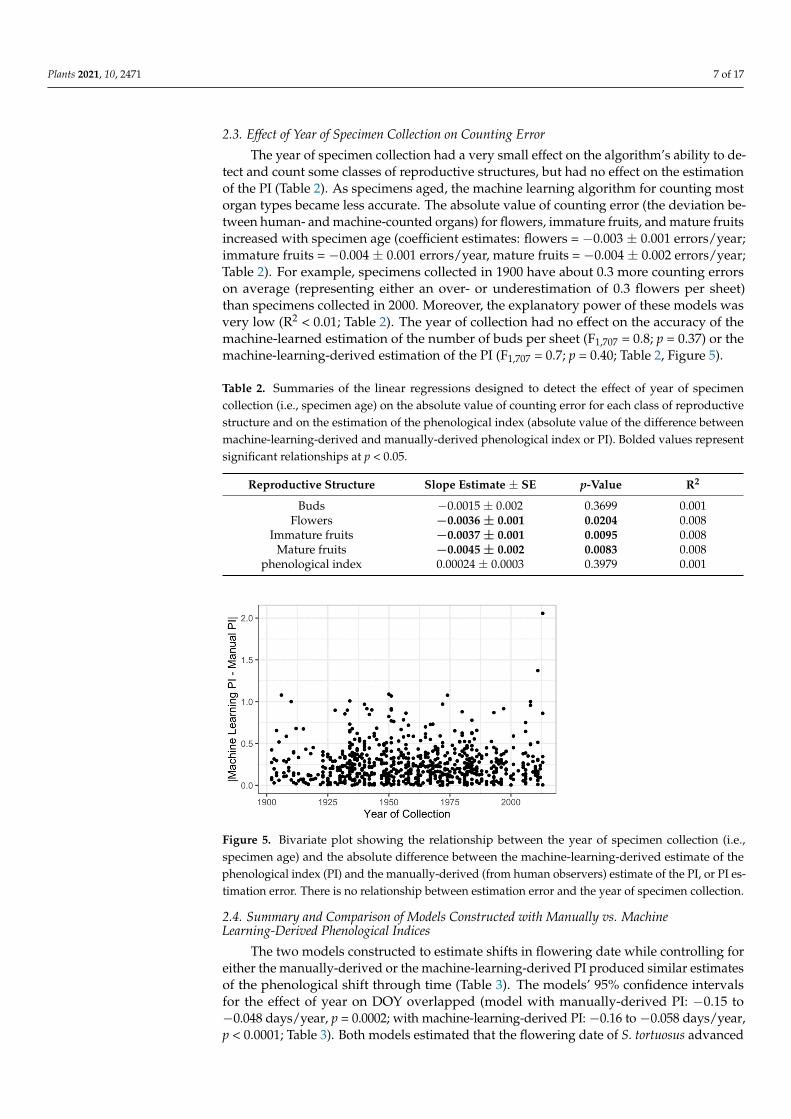
2.3. Effect of Year of Specimen Collection on Counting Error The year of specimen collection had a very small effect on the algorithm’s ability to

detect and count some classes of reproductive structures, but had no effect on the estimation of the PI (Table 2). As specimens aged, the machine learning algorithm for counting most organ types became less accurate. The absolute value of counting error (the deviation between human- and machine-counted organs) for flowers, immature fruits, and mature fruits increased with specimen age (coefficient estimates: flowers = −0.003 ± 0.001 errors/year; immature fruits = −0.004 ± 0.001 errors/year, mature fruits = −0.004 ± 0.002 errors/year; Table 2). For example, specimens collected in 1900 have about 0.3 more counting errors on average (representing either an over- or underestimation of 0.3 flowers per sheet) than specimens collected in 2000. Moreover, the explanatory power of these models was very low (R2 < 0.01; Table 2). The year of collection had no effect on the accuracy of the machine-learned estimation of the number of buds per sheet (F1,707 = 0.8; p = 0.37) or the machine-learning-derived estimation of the PI (F1,707 = 0.7; p = 0.40; Table 2, Figure 5).

Table 2. Summaries of the linear regressions designed to detect the effect of year of specimen collection (i.e., specimen age) on the absolute value of counting error for each class of reproductive structure and on the estimation of the phenological index (absolute value of the difference between machine-learning-derived and manually-derived phenological index or PI). Bolded values represent significant relationships at p < 0.05.

Reproductive Structure Slope Estimate ± SE p-Value R2 Buds −0.0015 ± 0.002 0.3699 0.001

Flowers −0.0036 ± 0.001 0.0204 0.008 Immature fruits −0.0037 ± 0.001 0.0095 0.008

Figure 4. Bivariate plot showing the relationship between the phenological index (PI) as estimatedusing predicted counts vs. manual counts (counted by human observers). The solid gray line denotesthe linear regression between the two estimates of PI. The dashed black line shows a hypothetical 1:1relationship where the two estimates result in the same PI value. Summaries for the regression canbe found in Table S2.

Plants 2021, 10, 2471 7 of 17

2.3. Effect of Year of Specimen Collection on Counting Error

The year of specimen collection had a very small effect on the algorithm’s ability to de-tect and count some classes of reproductive structures, but had no effect on the estimationof the PI (Table 2). As specimens aged, the machine learning algorithm for counting mostorgan types became less accurate. The absolute value of counting error (the deviation be-tween human- and machine-counted organs) for flowers, immature fruits, and mature fruitsincreased with specimen age (coefficient estimates: flowers = −0.003 ± 0.001 errors/year;immature fruits = −0.004 ± 0.001 errors/year, mature fruits = −0.004 ± 0.002 errors/year;Table 2). For example, specimens collected in 1900 have about 0.3 more counting errorson average (representing either an over- or underestimation of 0.3 flowers per sheet)than specimens collected in 2000. Moreover, the explanatory power of these models wasvery low (R2 < 0.01; Table 2). The year of collection had no effect on the accuracy of themachine-learned estimation of the number of buds per sheet (F1,707 = 0.8; p = 0.37) or themachine-learning-derived estimation of the PI (F1,707 = 0.7; p = 0.40; Table 2, Figure 5).

Table 2. Summaries of the linear regressions designed to detect the effect of year of specimencollection (i.e., specimen age) on the absolute value of counting error for each class of reproductivestructure and on the estimation of the phenological index (absolute value of the difference betweenmachine-learning-derived and manually-derived phenological index or PI). Bolded values representsignificant relationships at p < 0.05.

Reproductive Structure Slope Estimate ± SE p-Value R2

Buds −0.0015 ± 0.002 0.3699 0.001Flowers −0.0036 ± 0.001 0.0204 0.008

Immature fruits −0.0037 ± 0.001 0.0095 0.008Mature fruits −0.0045 ± 0.002 0.0083 0.008

phenological index 0.00024 ± 0.0003 0.3979 0.001

Plants 2021, 10, x FOR PEER REVIEW 9 of 19

Mature fruits −0.0045 ± 0.002 0.0083 0.008 phenological index 0.00024 ± 0.0003 0.3979 0.001

Figure 5. Bivariate plot showing the relationship between the year of specimen collection (i.e., specimen age) and the absolute difference between the machine-learning-derived estimate of the phenological index (PI) and the manually-derived (from human observers) estimate of the PI, or PI estimation error. There is no relationship between estimation error and the year of specimen collection.

2.4. Summary and Comparison of Models Constructed with Manually vs. Machine Learning-Derived Phenological Indices

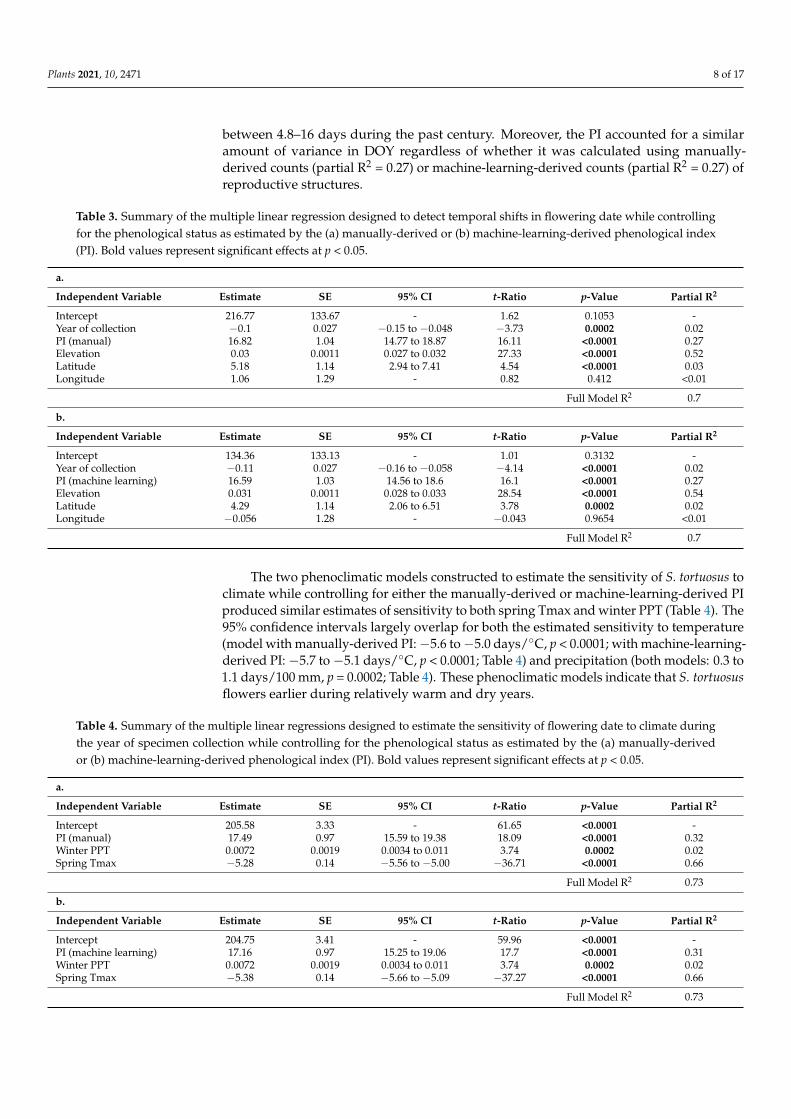
The two models constructed to estimate shifts in flowering date while controlling for either the manually-derived or the machine-learning-derived PI produced similar estimates of the phenological shift through time (Table 3). The models’ 95% confidence intervals for the effect of year on DOY overlapped (model with manually-derived PI: −0.15 to −0.048 days/year, p = 0.0002; with machine-learning-derived PI: −0.16 to −0.058 days/year, p < 0.0001; Table 3). Both models estimated that the flowering date of S. tortuosus advanced between 4.8–16 days during the past century. Moreover, the PI accounted for a similar amount of variance in DOY regardless of whether it was calculated using manually-derived counts (partial R2 = 0.27) or machine-learning-derived counts (partial R2 = 0.27) of reproductive structures.

Table 3. Summary of the multiple linear regression designed to detect temporal shifts in flowering date while controlling for the phenological status as estimated by the (a) manually-derived or (b) machine-learning-derived phenological index (PI). Bold values represent significant effects at p < 0.05.

a.

Independent Variable Estimate SE 95% CI t-Ratio p-Value Partial R2 Intercept 216.77 133.67 - 1.62 0.1053 - Year of collection −0.1 0.027 −0.15 to −0.048 −3.73 0.0002 0.02 PI (manual) 16.82 1.04 14.77 to 18.87 16.11 <0.0001 0.27 Elevation 0.03 0.0011 0.027 to 0.032 27.33 <0.0001 0.52 Latitude 5.18 1.14 2.94 to 7.41 4.54 <0.0001 0.03 Longitude 1.06 1.29 - 0.82 0.412 <0.01 Full Model R2 0.7 b.

Independent Variable Estimate SE 95% CI t-Ratio p-Value Partial R2 Intercept 134.36 133.13 - 1.01 0.3132 - Year of collection −0.11 0.027 −0.16 to −0.058 −4.14 <0.0001 0.02

Figure 5. Bivariate plot showing the relationship between the year of specimen collection (i.e.,specimen age) and the absolute difference between the machine-learning-derived estimate of thephenological index (PI) and the manually-derived (from human observers) estimate of the PI, or PI es-timation error. There is no relationship between estimation error and the year of specimen collection.

2.4. Summary and Comparison of Models Constructed with Manually vs. MachineLearning-Derived Phenological Indices

The two models constructed to estimate shifts in flowering date while controlling foreither the manually-derived or the machine-learning-derived PI produced similar estimatesof the phenological shift through time (Table 3). The models’ 95% confidence intervalsfor the effect of year on DOY overlapped (model with manually-derived PI: −0.15 to−0.048 days/year, p = 0.0002; with machine-learning-derived PI: −0.16 to −0.058 days/year,p < 0.0001; Table 3). Both models estimated that the flowering date of S. tortuosus advanced

Plants 2021, 10, 2471 8 of 17

between 4.8–16 days during the past century. Moreover, the PI accounted for a similaramount of variance in DOY regardless of whether it was calculated using manually-derived counts (partial R2 = 0.27) or machine-learning-derived counts (partial R2 = 0.27) ofreproductive structures.

Table 3. Summary of the multiple linear regression designed to detect temporal shifts in flowering date while controllingfor the phenological status as estimated by the (a) manually-derived or (b) machine-learning-derived phenological index(PI). Bold values represent significant effects at p < 0.05.

a.

Independent Variable Estimate SE 95% CI t-Ratio p-Value Partial R2

Intercept 216.77 133.67 - 1.62 0.1053 -Year of collection −0.1 0.027 −0.15 to −0.048 −3.73 0.0002 0.02PI (manual) 16.82 1.04 14.77 to 18.87 16.11 <0.0001 0.27Elevation 0.03 0.0011 0.027 to 0.032 27.33 <0.0001 0.52Latitude 5.18 1.14 2.94 to 7.41 4.54 <0.0001 0.03Longitude 1.06 1.29 - 0.82 0.412 <0.01

Full Model R2 0.7

b.

Independent Variable Estimate SE 95% CI t-Ratio p-Value Partial R2

Intercept 134.36 133.13 - 1.01 0.3132 -Year of collection −0.11 0.027 −0.16 to −0.058 −4.14 <0.0001 0.02PI (machine learning) 16.59 1.03 14.56 to 18.6 16.1 <0.0001 0.27Elevation 0.031 0.0011 0.028 to 0.033 28.54 <0.0001 0.54Latitude 4.29 1.14 2.06 to 6.51 3.78 0.0002 0.02Longitude −0.056 1.28 - −0.043 0.9654 <0.01

Full Model R2 0.7

The two phenoclimatic models constructed to estimate the sensitivity of S. tortuosus toclimate while controlling for either the manually-derived or machine-learning-derived PIproduced similar estimates of sensitivity to both spring Tmax and winter PPT (Table 4). The95% confidence intervals largely overlap for both the estimated sensitivity to temperature(model with manually-derived PI: −5.6 to −5.0 days/◦C, p < 0.0001; with machine-learning-derived PI: −5.7 to −5.1 days/◦C, p < 0.0001; Table 4) and precipitation (both models: 0.3 to1.1 days/100 mm, p = 0.0002; Table 4). These phenoclimatic models indicate that S. tortuosusflowers earlier during relatively warm and dry years.

Table 4. Summary of the multiple linear regressions designed to estimate the sensitivity of flowering date to climate duringthe year of specimen collection while controlling for the phenological status as estimated by the (a) manually-derivedor (b) machine-learning-derived phenological index (PI). Bold values represent significant effects at p < 0.05.

a.

Independent Variable Estimate SE 95% CI t-Ratio p-Value Partial R2

Intercept 205.58 3.33 - 61.65 <0.0001 -PI (manual) 17.49 0.97 15.59 to 19.38 18.09 <0.0001 0.32Winter PPT 0.0072 0.0019 0.0034 to 0.011 3.74 0.0002 0.02Spring Tmax −5.28 0.14 −5.56 to −5.00 −36.71 <0.0001 0.66

Full Model R2 0.73

b.

Independent Variable Estimate SE 95% CI t-Ratio p-Value Partial R2

Intercept 204.75 3.41 - 59.96 <0.0001 -PI (machine learning) 17.16 0.97 15.25 to 19.06 17.7 <0.0001 0.31Winter PPT 0.0072 0.0019 0.0034 to 0.011 3.74 0.0002 0.02Spring Tmax −5.38 0.14 −5.66 to −5.09 −37.27 <0.0001 0.66

Full Model R2 0.73

Plants 2021, 10, 2471 9 of 17

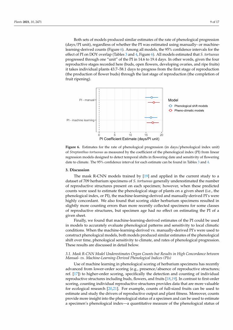
Both sets of models produced similar estimates of the rate of phenological progression(days/PI unit), regardless of whether the PI was estimated using manually- or machine-learning-derived counts (Figure 6). Among all models, the 95% confidence intervals for theeffect of PI on DOY overlap (Tables 3 and 4, Figure 6). All models estimated that S. tortuosusprogressed through one “unit” of the PI in 14.6 to 19.4 days. In other words, given the fourreproductive stages recorded here (buds, open flowers, developing ovaries, and ripe fruits)it takes individual plants 43.7–58.1 days to progress from the first stage of reproduction(the production of flower buds) through the last stage of reproduction (the completion offruit ripening).

Plants 2021, 10, x FOR PEER REVIEW 11 of 19

Figure 6. Estimates for the rate of phenological progression (in days/phenological index unit) of Streptanthus tortuosus as measured by the coefficient of the phenological index (PI) from linear regression models designed to detect temporal shifts in flowering date and sensitivity of flowering date to climate. The 95% confidence interval for each estimate can be found in Tables 3 and 4.

3. Discussion The mask R-CNN models trained by [19] and applied in the current study to a dataset

of 709 herbarium specimens of S. tortuosus generally underestimated the number of reproductive structures present on each specimen; however, when these predicted counts were used to estimate the phenological stage of plants on a given sheet (i.e., the phenological index, or PI), the machine-learning-derived and manually-derived PI’s were highly concordant. We also found that scoring older herbarium specimens resulted in slightly more counting errors than more recently collected specimens for some classes of reproductive structures, but specimen age had no effect on estimating the PI of a given sheet.

Finally, we found that machine-learning-derived estimates of the PI could be used in models to accurately evaluate phenological patterns and sensitivity to local climatic conditions. When the machine-learning-derived vs. manually-derived PI’s were used to construct phenological models, both models produced similar estimates of the phenological shift over time, phenological sensitivity to climate, and rates of phenological progression. These results are discussed in detail below.

3.1. Mask R-CNN Model Underestimates Organ Counts but Results in High Concordance between Manual- vs. Machine-Learning-Derived Phenological Indices (PIs)

Use of machine learning in phenological scoring of herbarium specimens has recently advanced from lower-order scoring (e.g., presence/absence of reproductive structures; ref. [17]) to higher-order scoring, specifically the detection and counting of individual reproductive structures including buds, flowers, and fruits [18,19]. In contrast to first-order scoring, counting individual reproductive structures provides data that are more valuable for ecological research [20,21]. For example, counts of full-sized fruits can be used to estimate and study the drivers of reproductive output and plant fitness. Moreover, counts provide more insight into the phenological status of a specimen and can be used to estimate a specimen’s phenological index—a quantitative measure of the phenological status of an herbarium specimen. The PI can be included as a predictor variable in phenological models to control statistically for variation in status among specimens when designing models to examine the factors influencing specimen collection date [13,14].

In the current study, the machine-learning algorithm generally underestimated the true number of reproductive structures present on each herbarium specimen of S. tortuosus (as counted manually by human scorers), and the number of counting errors was greater and more variable when more organs were present on a given sheet (Figures 1 and 2). This underestimation was more evident for counts of buds and flowers than for immature and mature fruits (Table 1). Davis et al. [18] used a similar machine-learning

Figure 6. Estimates for the rate of phenological progression (in days/phenological index unit)of Streptanthus tortuosus as measured by the coefficient of the phenological index (PI) from linearregression models designed to detect temporal shifts in flowering date and sensitivity of floweringdate to climate. The 95% confidence interval for each estimate can be found in Tables 3 and 4.

3. Discussion

The mask R-CNN models trained by [19] and applied in the current study to adataset of 709 herbarium specimens of S. tortuosus generally underestimated the numberof reproductive structures present on each specimen; however, when these predictedcounts were used to estimate the phenological stage of plants on a given sheet (i.e., thephenological index, or PI), the machine-learning-derived and manually-derived PI’s werehighly concordant. We also found that scoring older herbarium specimens resulted inslightly more counting errors than more recently collected specimens for some classesof reproductive structures, but specimen age had no effect on estimating the PI of agiven sheet.

Finally, we found that machine-learning-derived estimates of the PI could be usedin models to accurately evaluate phenological patterns and sensitivity to local climaticconditions. When the machine-learning-derived vs. manually-derived PI’s were used toconstruct phenological models, both models produced similar estimates of the phenologicalshift over time, phenological sensitivity to climate, and rates of phenological progression.These results are discussed in detail below.

3.1. Mask R-CNN Model Underestimates Organ Counts but Results in High Concordance betweenManual- vs. Machine-Learning-Derived Phenological Indices (PIs)

Use of machine learning in phenological scoring of herbarium specimens has recentlyadvanced from lower-order scoring (e.g., presence/absence of reproductive structures;ref. [17]) to higher-order scoring, specifically the detection and counting of individualreproductive structures including buds, flowers, and fruits [18,19]. In contrast to first-orderscoring, counting individual reproductive structures provides data that are more valuablefor ecological research [20,21]. For example, counts of full-sized fruits can be used toestimate and study the drivers of reproductive output and plant fitness. Moreover, countsprovide more insight into the phenological status of a specimen and can be used to estimatea specimen’s phenological index—a quantitative measure of the phenological status of

Plants 2021, 10, 2471 10 of 17

an herbarium specimen. The PI can be included as a predictor variable in phenologicalmodels to control statistically for variation in status among specimens when designingmodels to examine the factors influencing specimen collection date [13,14].

In the current study, the machine-learning algorithm generally underestimated thetrue number of reproductive structures present on each herbarium specimen of S. tortuosus(as counted manually by human scorers), and the number of counting errors was greaterand more variable when more organs were present on a given sheet (Figures 1 and 2). Thisunderestimation was more evident for counts of buds and flowers than for immature andmature fruits (Table 1). Davis et al. [18] used a similar machine-learning approach to detectand count reproductive structures on over 3000 herbarium specimens representing sixcommon wildflower species native to the eastern United States. In contrast to the currentstudy, their models produced more accurate counts of flowers and fruits than of buds. Intheir study, they found that detection and counting of buds was difficult for two reasons.First, very few training specimens (~10%) had buds represented on plants. Second, budswere smaller in size, and their visual appearance was less distinct than either flowers orfruits. Their results suggest that the accuracy of counting various classes of reproductivestructures may vary among species and depends on the morphological distinctivenessamong classes.

In the current study, the underestimation of organs among all classes may be dueto two factors. First, as more reproductive structures are present on an individual sheet,they tend to overlap and become crowded in addition to other occlusions related to theoverlapping of many stems or the presence of tape, which makes their detection moreprone to error (Figure 3). This may be especially true for buds, which tend to occurin dense clusters at branch tips. Second, specimens in the training dataset had fewerreproductive structures than those in the test dataset (Table S1). Because annotatinghundreds of reproductive structures for training datasets is very time intensive, we choseto annotate specimens with a moderate number of structures per sheet and those withrelatively few overlapping structures for which human observers could provide accuratecounts. Thus, test specimens with more reproductive structures than those used to trainthe model were more prone to counting error when scored. A more representative samplefor training (in terms of number of organs per sheet, degree of organ overlap, etc.) mayhave resulted in more accurate counts of reproductive structures but would have requireda substantial time investment. Future researchers will have to balance time investmentin annotating training specimens with the goals of the study, because relative abundancerather than exact counts of reproductive structures may be sufficient to meet the goals ofthe project, as was the case for the study presented here and discussed below.

Although the machine-learning model generally underestimated the number of repro-ductive structures present on specimens, when predicted counts were used to calculatethe phenological index (PI), they were highly concordant with the manually-derived PIs(Figure 4). Because estimating the PI relies on the proportions of reproductive structures ineach class rather than on the precise counts, the machine-learning-derived PIs were similarto those derived from manual counts (Figure 4).

The current study demonstrates that machine-learning-derived counts of reproductiveorgans using an object detection approach can be used to accurately estimate a quantitativemeasure of a herbarium specimen’s phenological status; however, this attribute can beestimated using other machine-learning approaches as well. In contrast to this study,Lorieul et al. [17] used a global visual or “glance” machine-learning approach (basedon a ResNet50 deep-learning model) to quantify phenological status using an imageclassification task in which each of the targeted visual classes was one of nine codedphenophases defined by the relative proportions of heads in bud, flower, or fruit presenton individual herbarium specimens of the Asteraceae. For example, a specimen withno heads in bud and 50% of heads in flower and fruit was given a phenophase scoreof seven, indicating that it was relatively late in its phenological progression [22]. Thisglobal visual approach was evaluated using 20,371 herbarium specimens representing

Plants 2021, 10, 2471 11 of 17

139 Asteraceae species and aimed to classify each specimen into one of the nine distinctphenophases. The classification accuracy among the phenophases varied from 8.6% to78.9%, with phenophase nine (representing 100% heads in fruit) being the most accuratelyclassified phenophase. This study demonstrates that counting individual reproductivestructures is not always necessary for the automated quantification of phenological status.This result may be relevant for studies where performing an object segmentation task isimpractical. For example, a global visual approach may be especially useful when scoringspecies with compound reproductive structures (e.g., heads in the Asteraceae family) wherecounting individual organs is challenging.

3.2. Low Impact of the Specimen Age on Counting Error

Herbarium specimens have recently emerged as reliable sources with which to detectand track phenological change through time [6,7,11]. As such, older specimens, specificallythose collected before the onset of contemporary climate change, are critical for these typesof studies. However, no studies have been designed to test whether older specimens can bereliably scored by machine learning. In this study, we found that the specimen collectionyear had little effect on the counting error of each class of reproductive structures (Table 2),and no effect on the accuracy of PI estimates (Figure 5).

This is the first study to demonstrate that machine learning can be used to accuratelyestimate the phenological status of older herbarium specimens. Importantly, our trainingdataset included specimens collected as early as 1899 (Table S1). Including a broad rangeof collection years in training datasets will likely yield more accurate scores for olderspecimens and prevent any type of temporal bias in scoring that could occur otherwise.Future researchers interested in using herbarium specimens to detect phenological shifts inresponse to recent climate change should consider including older specimens in their train-ing dataset to capture some of the color and morphological changes that occur as herbariumspecimens are stored for long periods of time. These considerations may be vital to produc-ing accurate estimates of phenological shifts using machine-learning-derived scores.

3.3. Machine-Learning-Derived Estimates of the Phenological Status Can Be Used to AssessEcological Patterns

Herbarium records are important sources of phenological data and can be used toreliably assess ecological patterns; however, no previous studies have been designed totest whether machine-learning-derived phenological scores of herbarium records can beused to accurately estimate such patterns. In the current study, we found that includingmachine-learning-derived PIs as predictor variables in phenological models produce simi-lar estimates of the phenological sensitivity to climate, temporal shifts in flowering time,and the rate of phenological progression (as estimated by the coefficient of the PI or days/PIunit; Tables 3 and 4, Figure 6) as models based on data provided by human observers.Moreover, the PI accounted for a similar amount of variance in DOY regardless of whetherit was estimated by human scorers or by machine-learning models (Tables 3 and 4).

Our results demonstrate that machine-learning-derived PIs can be reliably used as apredictor variable in phenological models to (1) control statistically for variation amongspecimens in their phenological status and (2) estimate the rate of phenological progression(Tables 3 and 4, Figure 6). However, because we found that the machine-learning modelgenerally underestimated the exact number of reproductive organs present on an individualherbarium specimen, phenological scores determined using the relative abundance oforgans, rather than exact counts, may be more reliable when using machine learning to scorespecimens [13,17]. Use of machine learning could accelerate the process of phenologicaldata extraction and scoring, especially if models trained on one species can be transferredto another [18]; however, more work is needed to determine the reliability of model transferto different species.

Plants 2021, 10, 2471 12 of 17

3.4. Future Directions

Creating masks to train object detection in machine learning models is a time intensiveprocess; however, the ability to transfer models trained on one species to a closely relatedand morphological species would enhance our capacity to extract phenological data fromimaged herbarium specimens. Davis et al. [18] showed that Mask R-CNN models trainedon specimen data of one species can be used to accurately detect and count phenologicalfeatures of a related species. They suggested that morphological similarity between speciesmay be a better guide for transferability success than phylogenetic relatedness, and thatresearchers should consider using morphological trait databases to estimate model trans-ferability potential. Many Streptanthus species have morphologically similar reproductivestructures, and the transferability of the model developed in the current study to othermembers of the genus will likely generate accurate estimates of specimen PIs.

Community science or crowd-based approaches for scoring specimens could also beleveraged to extend the use of machine learning in phenological research [16]. Crowd-basedapproaches that engage a large community of non-experts to score herbarium specimens area reliable way to extract phenological data from herbarium specimens while also providinga large amount of vital training data [18]. A large amount of high-quality training dataare key to the performance of automated detection models such as mask R-CNN. Theimplementation of enrichment and validation data derived from automated predictionscould quickly increase the diversity and volume of training data. For example, specimensthat have been scored by machine learning with high confidence could then be validatedby human scorers, which could enrich the training data and increase the diversity of visualcontexts on which models are trained and lead to the generation of more robust models.Finally, herbarium specimens scored using an object-detection-based approach generatemasks of individual reproductive structures that can be used to measure the shape andsize of individual organs (Figure 3). These phenotypic data could then be leveraged tostudy drivers of variation in shape and size of organs or to construct morphological traitdatabases (e.g., [23]).

4. Materials and Methods4.1. Assembling Herbarium Records and Manual Phenological Scoring

We assembled and manually scored the phenological status of 1138 herbarium recordsfrom seven herbaria (CAS, CHSC, DAV, OBI, RSA, SFV, and UCJEPS). We extracted the dayof year of specimen collection (DOY) from the collection information on the label of eachherbarium specimen. The DOY, which can range from 1 (1 January) to 365 (31 December),is a widely used estimate of flowering date derived from herbarium specimens and is usedcommonly as a response variable when estimating sensitivity of flowering date to climateand shifts in flowering time in phenological studies [6,11].

Specimens were then scored using the ImageJ scoring protocol and phenophasedefinitions described in Love et al. [13]. We used the Cell Counter Plug-in availablethrough ImageJ to score each specimen manually by placing a colored marker on eachbud, flower, immature fruit, and mature fruit. ImageJ summed the number of markersper category of reproductive structure on each sheet, and saved the x-y coordinates of themarker on each image. These manually placed markers were subsequently used to annotateimages for training the Mask R-CNN model (described in detail below and in [19]).

The manual counts were then used to calculate a quantitative estimate of the phenolog-ical stage of each herbarium record: the phenological index, or PI [13]. The PI is designedto be included as a predictor variable in regression models to control statistically for varia-tion in phenological status among herbarium records when estimating the sensitivity offlowering date to climate or shifts in flowering time in response to contemporary climatechange. To calculate the PI, each class of reproductive organ is assigned an index valuefrom 1–4 that represents the degree of phenological progression (buds = 1, flowers = 2,

Plants 2021, 10, 2471 13 of 17

immature fruits = 3, and mature fruits = 4). The proportion of reproductive structures ineach class is then used to calculate the PI per sheet using the following equation:

Phenological Index (PI) =4

∑i=1

Pxi (1)

where Px is the proportion of reproductive units in each class, and i represents the indexvalue assigned to each class of reproductive structure. A specimen with a PI of 1 wouldbe bearing only buds, indicating that the specimen was at an early stage of phenologicalprogression when collected. In contrast, a specimen with PI value of 4 would be bearingonly mature fruits and would indicate that the specimen was collected at a late reproductivestage. Specimens with values of the PI between 1 and 4 would typically be bearing acombination of at least two of the four classes of reproductive structures used in the currentstudy. Including the PI as a predictor variable in linear models designed to detect the effectsof local climate or year on the day of year of specimen collection is useful because the valueof PI is highly positively correlated with DOY (controlling for variation in local climate)and therefore contributes significantly to the model R2. All else being equal, specimenswith low values of the PI were collected earlier in the growing season than those with highvalues of the PI. In addition, the regression coefficient associated with the PI provides anestimate of how many days it takes for plants to increase their PI by a value of one (seeResults section for an example using the data analyzed here).

Next, we georeferenced each specimen by either downloading the latitude and longi-tude for that record from the California Consortium of Herbaria (CCH2; www.cch2.org(accessed on 3 March 2018)) or using the written description of the collection location toderive coordinates using GEOLocate (www.geo-locate.org (accessed on 3 March 2018)),a platform for georeferencing natural history specimens or electronic records. Each setof coordinates was also associated with an error radius (in meters) that represented theuncertainty of each location. After georeferencing, we excluded records with an errorradius greater than 4000 m and duplicate records. This resulted in a set of 709 specimensthat were then scored using the trained algorithm.

Extracting Climate Data

For each of the georeferenced specimen records, we extracted from ClimateNA [24]two climate variables that are known to be associated with flowering date in S. tortuosus:the maximum spring temperature (spring Tmax) and the cumulative winter precipitation(winter PPT) during the year of specimen collection [13,14]. ClimateNA is a data sourcethat downscales gridded PRISM data to scale-free point locations. While it is possible thatother climatic parameters may be better at predicting the flowering time of this species,testing all possible variables (and selecting the model of best fit) was beyond the scopeof this study; our goal was to select a reasonable model to use in order to compare theperformance of models using data obtained from a machine learning algorithm vs. fromhuman observers.

4.2. Machine Learning Methods4.2.1. Training Dataset

We uploaded images of herbarium specimens into COCO Annotator (https://github.com/jsbroks/coco-annotator (accessed on 2 February 2019), a web-based tool for object seg-mentation), in order to manually draw the full outline of each reproductive structure. Thisallowed us to capture the full shape of each reproductive organ identified on each specimen.When structures overlapped on the specimen, only the structure in the foreground wasannotated, resulting in the exclusion of background structures from the segmentation inthat part of the image. A total of 1036 reproductive structures from 21 herbarium specimenswere annotated (flower buds (279), flowers (349), immature fruits (196), and mature fruits(212)). This dataset is freely available on the Zenodo platform [25].

Plants 2021, 10, 2471 14 of 17

4.2.2. CNN Training and Prediction

For this study, we used the model trained by Goëau et al. [19]. This fine-graineddetection method is based on the mask R-CNN architecture [26], which has demonstratedits robustness and efficiency in instance segmentation tasks and challenges such as MSCOCO (Microsoft Common Objects in Context; [27]). This architecture used Facebook’smask R-CNN framework [28] implemented with PyTorch [29]. Goëau et al. [19] choseResNet-50 as the backbone CNN and the Feature Pyramid Networks [30] for instancesegmentation. The selection of the number of training iterations was made based on theempirical observation of the model’s training performance. The details of the traininghyperparameters are provided in Appendix A, and for a full discussion of the evaluationof the mask R-CNN model used in this study, see Goëau et al. [19].

4.3. Model Evaluation and Statistical Analyses4.3.1. Evaluation of Machine Learning Model Predictions

We evaluated the concordance between manual counts and predicted counts from themachine learning model in two ways [18]. First, we calculated the counting error (ei,k) perclass of reproductive organ (k) on each herbarium sheet (i), which is defined as the differencebetween the number of organs counted manually by human observers (ci,k) and the numberpredicted by the machine learning model (ci,k). We used the following equation:

ei,k = ci,k − ci,k (2)

where k represents buds, flowers, immature fruits, or mature fruits. Positive counting errorsrepresent cases in which the model overestimates the number of structures per sheet, whilenegative counting errors represent cases in which the model underestimates the number ofstructures. We also assessed whether the total number of reproductive structures per sheetaffected the degree of counting error by constructing box plots.

Second, we calculated the mean absolute error (MAE) per class of reproductive struc-ture, which measures the mean absolute error per class of reproductive structure across allsheets (N). We used the following equation:

MAE =1N ∑

i∑k

∣∣ei,k∣∣ (3)

4.3.2. Statistical Analysis

We calculated the Pearson correlation coefficients between manual- and machine-learning-derived counts to assess their concordance for each class of reproductive organ aswell as for the PI. We also fit a linear regression to these relationships. To determine howthe number of organs present on each sheet affected the algorithm’s ability to accuratelycount them, we plotted the distribution (as box plots) of count errors for each of five rangesof reproductive organs present (e.g., 0–9 organs, 10–19 organs, etc.).

To determine whether the year of collection affected the model’s ability to accuratelycount the number of reproductive structures on each sheet, we constructed one linearmodel for each of the four organ classes that assessed the effect of year of collection on theabsolute value of the counting error. We used the absolute value of counting error in thisanalysis because we were interested in estimating the effect of year on the overall error rateand not whether the algorithm specifically over- or underestimates the organ count throughtime. We also used linear regression to assess whether the year of collection affected theestimation of the PI. To improve normality, the absolute value of counting error was log10transformed after adding 1 to each value, and the PI was square root transformed.

We constructed two sets of multivariate linear regression models (with two modelseach) to determine whether the PI derived from machine learning counts (or predictedcounts) could be used to construct models that accurately estimate (relative to the humanobservations) the rate of temporal shifts in flowering date (set 1) and the sensitivity of

Plants 2021, 10, 2471 15 of 17

flowering date to climate (set 2). Models in each set controlled for variation in phenologicalstatus among specimens by including the PI derived from either manual or predictedcounts, but otherwise included the same predictors. The first set of models (set 1) assessedthe effect of year on the DOY to determine the rate of phenological change (days/year),and included year, PI, elevation, latitude, and longitude as main effects. The second setof models (set 2) assessed the sensitivity of flowering date (DOY) to climate during theyear of specimen collection and included PI, cumulative winter precipitation, and springmaximum temperature. Temperature and precipitation have been demonstrated to affectflowering date in Streptanthus tortuosus where the date of specimen collection is used as aproxy for flowering date (Love et al., 2019; Love and Mazer, 2021). For both sets of models,we calculated the 95% confidence interval of each coefficient estimate as well as the partialR2 for each main effect.

Because both sets of models included the PI as a main effect, this allowed us tocompare the rate of phenological progression (days/PI unit) as estimated by the regressioncoefficient of the PI (whether the PI was estimated from manual or machine-learned counts)among all four models. We used the 95% confidence interval to evaluate whether theestimated rate of phenological progression differed between counting methods (manualvs. machine learning) or among models. All statistical analyses were conducted using Rversion 4.0.3 [31].

Supplementary Materials: The following are available online at https://www.mdpi.com/article/10.3390/plants10112471/s1, Figure S1: Map showing the distribution of the 709 Streptanthus tortuosusherbarium specimens used in this study (white points). Inset map shows the location of Californiawithin the United States of America (USA) and bolded black box shows the extent of the herbariumcollections displayed in the main map, Table S1: Comparison of the number of reproductive organs,phenological indices, plants/sheet, and year of collections between training and test datasets, Table S2:Summaries of the linear regressions designed to assess the concordance between manually vs.machine learning derived counts of reproductive organs and the phenological index.

Author Contributions: This project was conceptualized by all authors. P.B., H.G. and A.J. developedthe machine learning model and methodology to score herbarium specimens. N.L.R.L. and S.J.M. ledthe formal analysis effort and prepared the original draft of the manuscript. N.L.R.L., S.J.M., P.B.,H.G. and A.J. reviewed and edited the draft. All authors have read and agreed to the publishedversion of the manuscript.

Funding: This research received no external funding.

Institutional Review Board Statement: Not applicable.

Informed Consent Statement: Not applicable.

Data Availability Statement: All data used to conduct this study can be found at https://doi.org/10.5281/zenodo.5574675 (accessed on 18 October 2021).

Acknowledgments: The authors would like to thank Timothy (TJ) Sears, Allison Lane, Monica Lopez,Sarah Abrahem, Sophia Lau-Shum, and Kekai ‘O Kalani Akita for their help with scoring manyherbarium specimens. We would also like to thank the many botanists who collected Streptanthustortuosus during the past ~150 years and the numerous herbarium curators for maintaining thecollections used in this study.

Conflicts of Interest: The authors declare no conflict of interest.

Appendix A

Description of the hyperparameters used to train the mask R-CNN architecture:

• Input image size: Images are resized such that the longest edge is 2048 pixels and theshorter one is 1024 pixels, in order to have sufficient pixels related to small objectssuch as the buds (by default the mask R-CNN implementation used here considers alongest edge of 1024 pixels and a shorter one of 600 pixels).

Plants 2021, 10, 2471 16 of 17

• Anchor size and stride: Anchors are the raw regions of interest used by the regionproposal network to select the candidate bounding boxes for object detection. Wechose their size to guarantee that the targeted objects have their size covered. Theanchor size values were set to [32; 64; 128; 256; 512], the anchor stride values to [4; 8;16; 32; 64], and the anchor ratios to [0.5; 1; 2].

• Non-maximal suppression: The non-maximal suppression (NMS) quantifies the de-gree of overlap tolerated between two distinct objects (set to 0.5, the default value inthe mask R-CNN implementation used here).

The training of the model was run on an NVidia Geforce RTX 2080 Ti (NVidia Cor-poration, Santa Clara, CA, USA) using stochastic gradient descent with the followingparameters: batch size of 3, total number of max iterations limited to 70,000, and learningrate of 0.01. We trained our model for several periods of time and stopped training whenthe loss had stopped decreasing after more than two days. More specifically, we use atechnique called the “panda approach,” in which all training parameter choices were madeon the basis of the empirical observation of the model’s training performance. We useda warm-up strategy, where the learning rate increases linearly from 0.005 to 0.01 duringthe first 500 iterations. To improve robustness and minimize the variance of the model,we applied a large set of data augmentation techniques, including random horizontal,random rotations, and random variations on color contrast, saturation, brightness, and huecolor values.

References1. Ettinger, A.K.; Chamberlain, C.J.; Morales-Castilla, I.; Buonaiuto, D.M.; Flynn, D.F.B.; Savas, T.; Samaha, J.A.; Wolkovich, E.M.

Winter Temperatures Predominate in Spring Phenological Responses to Warming. Nat. Clim. Chang. 2020, 10, 1137–1142.[CrossRef]

2. Cook, B.I.; Wolkovich, E.M.; Parmesan, C. Divergent Responses to Spring and Winter Warming Drive Community Level FloweringTrends. Proc. Natl. Acad. Sci. USA 2012, 109, 9000–9005. [CrossRef]

3. Wolkovich, E.M.; Davies, T.J.; Schaefer, H.; Cleland, E.E.; Cook, B.I.; Travers, S.E.; Willis, C.G.; Davis, C.C. Temperature-DependentShifts in Phenology Contribute to the Success of Exotic Species with Climate Change. Am. J. Bot. 2013, 100, 1407–1421. [CrossRef]

4. Kudo, G.; Cooper, E.J. When Spring Ephemerals Fail to Meet Pollinators: Mechanism of Phenological Mismatch and Its Impacton Plant Reproduction. Proc. R. Soc. B Biol. Sci. 2019, 286, 20190573. [CrossRef]

5. Meineke, E.K.; Davies, T.J. Museum Specimens Provide Novel Insights into Changing Plant–Herbivore Interactions. Philos. Trans.R. Soc. B Biol. Sci. 2019, 374, 20170393. [CrossRef] [PubMed]

6. Willis, C.G.; Ellwood, E.R.; Primack, R.B.; Davis, C.C.; Pearson, K.D.; Gallinat, A.S.; Yost, J.M.; Nelson, G.; Mazer, S.J.; Rossington,N.L.; et al. Old Plants, New Tricks: Phenological Research Using Herbarium Specimens. Trends Ecol. Evol. 2017, 32, 531–546.[CrossRef] [PubMed]

7. Jones, C.A.; Daehler, C.C. Herbarium Specimens Can Reveal Impacts of Climate Change on Plant Phenology; a Review ofMethods and Applications. PeerJ 2018, 6, e4576. [CrossRef] [PubMed]

8. Pau, S.; Wolkovich, E.M.; Cook, B.I.; Davies, T.J.; Kraft, N.J.B.; Bolmgren, K.; Betancourt, J.L.; Cleland, E.E. Predicting Phenologyby Integrating Ecology, Evolution and Climate Science. Glob. Chang. Biol. 2011, 17, 3633–3643. [CrossRef]

9. Wolkovich, E.M.; Cook, B.I.; Davies, T.J. Progress towards an Interdisciplinary Science of Plant Phenology: Building Predictionsacross Space, Time and Species Diversity. New Phytol. 2014, 201, 1156–1162. [CrossRef] [PubMed]

10. Robbirt, K.M.; Davy, A.J.; Hutchings, M.J.; Roberts, D.L. Validation of Biological Collections as a Source of Phenological Datafor Use in Climate Change Studies: A Case Study with the Orchid Ophrys sphegodes: Herbarium Specimens for Climate ChangeStudies. J. Ecol. 2011, 99, 235–241. [CrossRef]

11. Davis, C.C.; Willis, C.G.; Connolly, B.; Kelly, C.; Ellison, A.M. Herbarium Records Are Reliable Sources of Phenological ChangeDriven by Climate and Provide Novel Insights into Species’ Phenological Cueing Mechanisms. Am. J. Bot. 2015, 102, 1599–1609.[CrossRef]

12. Meineke, E.K.; Davis, C.C.; Davies, T.J. The Unrealized Potential of Herbaria for Global Change Biology. Ecol. Monogr. 2018, 88,505–525. [CrossRef]

13. Love, N.L.R.; Park, I.W.; Mazer, S.J. A New Phenological Metric for Use in Pheno-climatic Models: A Case Study Using HerbariumSpecimens of Streptanthus tortuosus. Appl. Plant Sci. 2019, 7, e11276. [CrossRef] [PubMed]

14. Love, N.L.R.; Mazer, S.J. Region-Specific Phenological Sensitivities and Rates of Climate Warming Generate Divergent Shifts inFlowering Date across a Species’ Range. Am. J. Bot. 2021, 108, 1–16. [CrossRef] [PubMed]

15. Mazer, S.J.; Love, N.L.R.; Park, I.M.; Tadeo, R.P.; Elizabeth, R.M. Phenological Sensitivities to Climate Are Similar in Two ClarkiaCongeners: Indirect Evidence for Facilitation, Convergence, Niche Conservatism, or Genetic Constraints. Madroño 2022, in press.

Plants 2021, 10, 2471 17 of 17

16. Willis, C.G.; Law, E.; Williams, A.C.; Franzone, B.F.; Bernardos, R.; Bruno, L.; Hopkins, C.; Schorn, C.; Weber, E.; Park, D.S.; et al.CrowdCurio: An Online Crowdsourcing Platform to Facilitate Climate Change Studies Using Herbarium Specimens. New Phytol.2017, 215, 479–488. [CrossRef]

17. Lorieul, T.; Pearson, K.D.; Ellwood, E.R.; Goëau, H.; Molino, J.-F.; Sweeney, P.W.; Yost, J.M.; Sachs, J.; Mata-Montero, E.; Nelson,G.; et al. Toward a Large-Scale and Deep Phenological Stage Annotation of Herbarium Specimens: Case Studies from Temperate,Tropical, and Equatorial Floras. Appl. Plant Sci. 2019, 7, e01233. [CrossRef]

18. Davis, C.C.; Champ, J.; Park, D.S.; Breckheimer, I.; Lyra, G.M.; Xie, J.; Joly, A.; Tarapore, D.; Ellison, A.M.; Bonnet, P. A NewMethod for Counting Reproductive Structures in Digitized Herbarium Specimens Using Mask R-CNN. Front. Plant Sci. 2020,11, 1129. [CrossRef] [PubMed]

19. Goëau, H.; Mora-Fallas, A.; Champ, J.; Love, N.L.R.; Mazer, S.J.; Mata-Montero, E.; Joly, A.; Bonnet, P. A New Fine-grainedMethod for Automated Visual Analysis of Herbarium Specimens: A Case Study for Phenological Data Extraction. Appl. Plant Sci.2020, 8, e11368. [CrossRef]

20. Pearson, K.D.; Nelson, G.; Aronson, M.F.J.; Bonnet, P.; Brenskelle, L.; Davis, C.C.; Denny, E.G.; Ellwood, E.R.; Goëau, H.;Heberling, J.M.; et al. Machine Learning Using Digitized Herbarium Specimens to Advance Phenological Research. BioScience2020, 70, 610–620. [CrossRef]

21. Yost, J.M.; Sweeney, P.W.; Gilbert, E.; Nelson, G.; Guralnick, R.; Gallinat, A.S.; Ellwood, E.R.; Rossington, N.; Willis, C.G.; Blum,S.D.; et al. Digitization Protocol for Scoring Reproductive Phenology from Herbarium Specimens of Seed Plants. Appl. Plant Sci.2018, 6, e1022. [CrossRef] [PubMed]

22. Pearson, K.D. A New Method and Insights for Estimating Phenological Events from Herbarium Specimens. Appl. Plant Sci. 2019,7, e01224. [CrossRef] [PubMed]

23. Weaver, W.N.; Ng, J.; Laport, R.G. LeafMachine: Using Machine Learning to Automate Leaf Trait Extraction from DigitizedHerbarium Specimens. Appl. Plant Sci. 2020, 8, e11367. [CrossRef] [PubMed]

24. Wang, T.; Hamann, A.; Spittlehouse, D.; Carroll, C. Locally Downscaled and Spatially Customizable Climate Data for Historicaland Future Periods for North America. PLoS ONE 2016, 11, e0156720. [CrossRef]

25. Goëau, H.; Mora-Fallas, A.; Champ, J.; Love, N.L.R.; Mazer, S.; Mata-Montero, E.; Joly, A.; Bonnet, P. Fine-Grained AutomatedVisual Analysis of Herbarium Specimens for Phenological Data Extraction: An Annotated Dataset of Reproductive Organs inStrepanthus Herbarium Specimens. 2020. Available online: https://zenodo.org/record/3865263#.YZMUt7oRVPY (accessed on10 November 2021).

26. He, K.; Gkioxari, G.; Dollár, P.; Girshick, R. Mask R-CNN. In Proceedings of the IEEE International Conference on ComputerVision, Venice, Italy, 22–29 October 2017.

27. Lin, T.Y.; Maire, M.; Belongie, S.; Hays, J.; Perona, P.; Ramanan, D.; Dollár, P.; Zitnick, C.L. Microsoft COCO: Common Objects inContext; Springer: Cham, Switzerland, 2014; pp. 740–755.

28. Massa, F.; Girshick, R. Maskrcnn-Benchmark: Fast, Modular Reference Implementation of Instance Segmentation and ObjectDetection Algorithms in PyTorch. 2018. Available online: https://github.com/facebookresearch/maskrcnn-benchmark (accessedon 2 February 2019).

29. Paszke, A.; Gross, S.; Chintala, S.; Chanan, G.; Yang, E.; DeVito, Z.; Lin, Z.; Desmaison, A.; Antiga, L.; Lerer, A.; et al. AutomaticDifferentiation in PyTorch. In Proceedings of the 31st Conference on Neural Information Processing Systems (NIPS 2017), LongBeach, CA, USA, 9 December 2017.

30. Lin, T.Y.; Dollár, P.; Girshick, R.; He, K.; Hariharan, B.; Belongie, S. Feature Pyramid Networks for Object Detection. InProceedings of the IEEE International Conference on Computer Vision and Pattern Recognition, Honolulu, Hawaii, 21–26 July2017; pp. 2117–2125.

31. R Core Team. R: A Language and Environment for Statistical Computing; R Foundation for Statistical Computing: Vienna,Austria, 2020.