Mid-price prediction based on machine learning methods with ...
Upload
khangminh22Category
view
1download
0
Machine-Learning Applied Methods
Sebastián Mauricio Palacio
ADVERTIMENT. La consulta d’aquesta tesi queda condicionada a l’acceptació de les següents condicions d'ús: La difusió d’aquesta tesi per mitjà del servei TDX (www.tdx.cat) i a través del Dipòsit Digital de la UB (diposit.ub.edu) ha estat autoritzada pels titulars dels drets de propietat intel·lectual únicament per a usos privats emmarcats en activitats d’investigació i docència. No s’autoritza la seva reproducció amb finalitats de lucre ni la seva difusió i posada a disposició des d’un lloc aliè al servei TDX ni al Dipòsit Digital de la UB. No s’autoritza la presentació del seu contingut en una finestra o marc aliè a TDX o al Dipòsit Digital de la UB (framing). Aquesta reserva de drets afecta tant al resum de presentació de la tesi com als seus continguts. En la utilització o cita de parts de la tesi és obligat indicar el nom de la persona autora. ADVERTENCIA. La consulta de esta tesis queda condicionada a la aceptación de las siguientes condiciones de uso: La difusión de esta tesis por medio del servicio TDR (www.tdx.cat) y a través del Repositorio Digital de la UB (diposit.ub.edu) ha sido autorizada por los titulares de los derechos de propiedad intelectual únicamente para usos privados enmarcados en actividades de investigación y docencia. No se autoriza su reproducción con finalidades de lucro ni su difusión y puesta a disposición desde un sitio ajeno al servicio TDR o al Repositorio Digital de la UB. No se autoriza la presentación de su contenido en una ventana o marco ajeno a TDR o al Repositorio Digital de la UB (framing). Esta reserva de derechos afecta tanto al resumen de presentación de la tesis como a sus contenidos. En la utilización o cita de partes de la tesis es obligado indicar el nombre de la persona autora. WARNING. On having consulted this thesis you’re accepting the following use conditions: Spreading this thesis by the TDX (www.tdx.cat) service and by the UB Digital Repository (diposit.ub.edu) has been authorized by the titular of the intellectual property rights only for private uses placed in investigation and teaching activities. Reproduction with lucrative aims is not authorized nor its spreading and availability from a site foreign to the TDX service or to the UB Digital Repository. Introducing its content in a window or frame foreign to the TDX service or to the UB Digital Repository is not authorized (framing). Those rights affect to the presentation summary of the thesis as well as to its contents. In the using or citation of parts of the thesis it’s obliged to indicate the name of the author.

PhD in Economics
Seba
stiá
n M
auri
cio
Pala
cio
PhD
in E
cono
mic
s
Sebastián Mauricio Palacio
Machine-Learning Applied Methods
2020

Thesis title:
PhD student:
Sebastián Mauricio Palacio
Advisor:
Joan-Ramon Borrell
Date: February 2020
PhD in Economics
Machine-Learning Applied Methods

To Kine, Marcela and Antonia

iv

Acknowledgments
I was accepted to the PhD program at the Department of Econometrics, Statisticsand Applied Economics in May 2016. A lot of things have happened since that dayand many people have played a part in finally presenting my thesis.
I would first like to thank to my supervisor Joan-Ramon Borrell and my tutorMontserrat Guillen, whose invaluable contributions and guidance encouraged menever to give up. Ever since I did my Master’s degree, Joan-Ramon has had an openmind and given me the freedom and trust to follow my own path. For this I amgrateful. Also for all the encouragement and the precise comments on my work,and for always taking time to answer my numerous questions whether related to thethesis or not. Thank you both!
I would like to acknowledge Zurich Insurance Ltd for their financial support andfor letting me to conduct my research in their installations and providing me notonly with technological and data resources, but also giving me total freedom andflexibility. In particular, I owe gratitude to my colleagues in the Advanced Ana-lytics Department. Especially, I would like to thank to Cristina Rata for her trustand support, and Gledys Alexandra Sulbarán Goyo for her companionship in theworkplace since my first day at Zurich.
As well, I would like to say thank you to all the members of the Public PolicySection of the Universitat de Barcelona. From the start, I felt the friendly and wel-coming atmosphere in the department. The doors were always open and everybodywas always eager to help or give advice in time of need.
From UB I would like to thank Stephan Joseph and Francisco Robles both forinteresting academic discussions but also for all the good times in Barcelona. Iwould also like to thank my department colleagues: Carlitos, Max, Paula and Taniafor being amazing persons and for always being there with a smile.
I would also like to thank to UBEconomics, especially Jordi Roca who has helpedme with administrative issues from my first day as a PhD student.
Although the people mentioned above are very important in the process of fin-ishing this thesis, I would never have been able to finish it without the support fromfamily and friends. I wish to thank my family for always supporting and believingin me, who made all of this possible, especially mum and my grandma. To my dearfriends: Diego, Germán, Emanuel and Nacho. I really appreciate our friendship. Iwould never forget the day you traveled thousands of kilometers just to be with me.
Last but not least, to Kine Bjerke, my wife and the love of my life. You notonly moved far away from your family because of me but as well you have been bymy side throughout this entire process. I really do not know how all of this wouldhave been possible without you. There are not word that can express how much I
v

appreciate that you chose to spend your life with me.
vi

Contents
1 Introduction 11.1 Prediction versus Causal Inference . . . . . . . . . . . . . . . . . . 11.2 Why Machine Learning and Deep Learning? . . . . . . . . . . . . . 41.3 Structure and Objectives of this Thesis . . . . . . . . . . . . . . . . 5
2 Predicting Collusive Patterns in Electricity Markets 92.1 Introduction . . . . . . . . . . . . . . . . . . . . . . . . . . . . . . 92.2 Literature Review . . . . . . . . . . . . . . . . . . . . . . . . . . . 122.3 Case Study . . . . . . . . . . . . . . . . . . . . . . . . . . . . . . . 15
2.3.1 Forward Premium . . . . . . . . . . . . . . . . . . . . . . . 192.3.2 Sector Concentration . . . . . . . . . . . . . . . . . . . . . 202.3.3 Nord Pool . . . . . . . . . . . . . . . . . . . . . . . . . . . 21
2.4 Theoretical Model . . . . . . . . . . . . . . . . . . . . . . . . . . . 212.5 Methodology . . . . . . . . . . . . . . . . . . . . . . . . . . . . . 25
2.5.1 Price Dynamic in Electrical Markets . . . . . . . . . . . . . 262.5.2 Identification and Estimation Methods . . . . . . . . . . . . 27
2.6 Results . . . . . . . . . . . . . . . . . . . . . . . . . . . . . . . . . 292.6.1 Windows Choice . . . . . . . . . . . . . . . . . . . . . . . 302.6.2 Identification Strategy . . . . . . . . . . . . . . . . . . . . 322.6.3 The Effect of Mandated Auctions on Prices . . . . . . . . . 39
2.7 Conclusions and Policy Implications . . . . . . . . . . . . . . . . . 42
3 Machine Learning Forecasts of Public Transport Demand 553.1 Introduction . . . . . . . . . . . . . . . . . . . . . . . . . . . . . . 553.2 Case Study and Data . . . . . . . . . . . . . . . . . . . . . . . . . 59
3.2.1 SUBE . . . . . . . . . . . . . . . . . . . . . . . . . . . . . 623.2.2 Weather . . . . . . . . . . . . . . . . . . . . . . . . . . . . 633.2.3 Economics . . . . . . . . . . . . . . . . . . . . . . . . . . 63
3.3 Methodology . . . . . . . . . . . . . . . . . . . . . . . . . . . . . 633.3.1 Basic Statistics . . . . . . . . . . . . . . . . . . . . . . . . 633.3.2 Ordinary Least Squares . . . . . . . . . . . . . . . . . . . . 66
vii

Contents
3.3.3 SARIMAX . . . . . . . . . . . . . . . . . . . . . . . . . . 683.3.4 Machine Learning Algorithms . . . . . . . . . . . . . . . . 71
3.4 Results . . . . . . . . . . . . . . . . . . . . . . . . . . . . . . . . . 733.4.1 Interpretability . . . . . . . . . . . . . . . . . . . . . . . . 743.4.2 Predictive Power . . . . . . . . . . . . . . . . . . . . . . . 763.4.3 Demand Elasticity . . . . . . . . . . . . . . . . . . . . . . 76
3.5 Conclusions . . . . . . . . . . . . . . . . . . . . . . . . . . . . . . 81
4 Abnormal Pattern Prediction in the Insurance Market 834.1 Introduction . . . . . . . . . . . . . . . . . . . . . . . . . . . . . . 834.2 Data . . . . . . . . . . . . . . . . . . . . . . . . . . . . . . . . . . 864.3 Methodology . . . . . . . . . . . . . . . . . . . . . . . . . . . . . 87
4.3.1 Unsupervised Model Selection . . . . . . . . . . . . . . . . 884.3.2 Supervised Model Selection . . . . . . . . . . . . . . . . . 94
4.4 Results . . . . . . . . . . . . . . . . . . . . . . . . . . . . . . . . . 984.4.1 Performance . . . . . . . . . . . . . . . . . . . . . . . . . . 984.4.2 Investigation Office Validation . . . . . . . . . . . . . . . . 994.4.3 Dynamic Learning . . . . . . . . . . . . . . . . . . . . . . 100
4.5 Conclusion . . . . . . . . . . . . . . . . . . . . . . . . . . . . . . 1014.6 Appendix. Practical Example . . . . . . . . . . . . . . . . . . . . . 102
5 Risk Categorization and Self-Reported Mechanisms in AutomobileInsurance Markets 1075.1 Introduction . . . . . . . . . . . . . . . . . . . . . . . . . . . . . . 1075.2 Literature Review . . . . . . . . . . . . . . . . . . . . . . . . . . . 1105.3 Theoretical Model . . . . . . . . . . . . . . . . . . . . . . . . . . . 113
5.3.1 Self Selection Mechanism . . . . . . . . . . . . . . . . . . 1155.3.2 Risk Categorization . . . . . . . . . . . . . . . . . . . . . . 117
5.4 Data . . . . . . . . . . . . . . . . . . . . . . . . . . . . . . . . . . 1205.4.1 Description of the Data . . . . . . . . . . . . . . . . . . . . 1205.4.2 Target Variable: The Definition of Risk . . . . . . . . . . . 124
5.5 Methodology . . . . . . . . . . . . . . . . . . . . . . . . . . . . . 1265.6 Results . . . . . . . . . . . . . . . . . . . . . . . . . . . . . . . . . 130
5.6.1 Misreporting Behavior: Testable Implications . . . . . . . . 1305.6.2 Predicting Misreporting Behavior with Observable Charac-
teristic . . . . . . . . . . . . . . . . . . . . . . . . . . . . . 1325.6.3 Combining Self-Reported Data and Observables . . . . . . . 1335.6.4 Feature Importance of Risk . . . . . . . . . . . . . . . . . . 133
5.7 Conclusion . . . . . . . . . . . . . . . . . . . . . . . . . . . . . . 137
viii

5.8 Appendix . . . . . . . . . . . . . . . . . . . . . . . . . . . . . . . 1395.8.1 Clustering Observable Risk Variables . . . . . . . . . . . . 1395.8.2 Variational Autoencoder Model Validation . . . . . . . . . . 1425.8.3 Internal Cluster Validation Plots . . . . . . . . . . . . . . . 1485.8.4 Cluster Statistics Plots . . . . . . . . . . . . . . . . . . . . 1495.8.5 Network Architecture . . . . . . . . . . . . . . . . . . . . . 154
6 Conclusions 1556.1 Future Work . . . . . . . . . . . . . . . . . . . . . . . . . . . . . . 160Bibliography . . . . . . . . . . . . . . . . . . . . . . . . . . . . . . . . . 163
List of Figures
1.1 Data Volume Growth by Year in Zettabytes . . . . . . . . . . . . . 2
2.1 Auction Design . . . . . . . . . . . . . . . . . . . . . . . . . . . . 152.2 Main Factors Argued by the CNMC. Plots contain wind produc-
tion over total production, total demand (GWh), unavailable power(GW), international petrol price (USD per barrel) and internationalgas price (USD/BTU). . . . . . . . . . . . . . . . . . . . . . . . . . 18
2.3 Normal Data Test . . . . . . . . . . . . . . . . . . . . . . . . . . . 312.4 Abnormal Data Test . . . . . . . . . . . . . . . . . . . . . . . . . . 312.5 Parallel Trend . . . . . . . . . . . . . . . . . . . . . . . . . . . . . 352.6 Schematic Representation of Leads and Lags . . . . . . . . . . . . . 362.7 Armax Building-Model Process . . . . . . . . . . . . . . . . . . . . 472.8 Partial Autocorrelation and Autocorrelation Functions . . . . . . . . 492.9 Schematic Diagram of the LSTM unit with forget gates . . . . . . . 51
3.1 Domiciliary Mobility Survey (2013) . . . . . . . . . . . . . . . . . 603.2 Location of CABA . . . . . . . . . . . . . . . . . . . . . . . . . . 603.3 Weather Conditions in CABA (source INTA) . . . . . . . . . . . . 613.4 Number of Passengers by Day . . . . . . . . . . . . . . . . . . . . 613.5 Nominal and Real Fares Evolution . . . . . . . . . . . . . . . . . . 623.6 Multiplicative Decomposition . . . . . . . . . . . . . . . . . . . . . 643.7 Seasonality Pattern . . . . . . . . . . . . . . . . . . . . . . . . . . 643.8 Series Stationarity . . . . . . . . . . . . . . . . . . . . . . . . . . . 65
ix

List of Figures
3.9 Series Stationarity . . . . . . . . . . . . . . . . . . . . . . . . . . . 693.10 Elastic Net 5-Fold CV . . . . . . . . . . . . . . . . . . . . . . . . . 723.11 Sample Split . . . . . . . . . . . . . . . . . . . . . . . . . . . . . . 743.12 Economic Variables Evolution . . . . . . . . . . . . . . . . . . . . 783.13 Passenger (in millions) Before and After the Last Fare Increase . . . 783.14 Test Prediction . . . . . . . . . . . . . . . . . . . . . . . . . . . . . 793.15 Test Prediction with Random Forest . . . . . . . . . . . . . . . . . 803.16 SARIMAX: Expanded Elasticity . . . . . . . . . . . . . . . . . . . 81
4.1 Possible clusters . . . . . . . . . . . . . . . . . . . . . . . . . . . . 894.2 Desired Threshold . . . . . . . . . . . . . . . . . . . . . . . . . . . 894.3 Cluster Example Output. . . . . . . . . . . . . . . . . . . . . . . . 92
5.1 Public Information Equilibrium . . . . . . . . . . . . . . . . . . . . 1145.2 Private Information Equilibrium . . . . . . . . . . . . . . . . . . . 1155.3 Semi-Private Information Equilibrium . . . . . . . . . . . . . . . . 1165.4 Policy Subscription . . . . . . . . . . . . . . . . . . . . . . . . . . 1215.5 Simulated and Adjusted Bonus . . . . . . . . . . . . . . . . . . . . 1265.6 Anomaly Distribution . . . . . . . . . . . . . . . . . . . . . . . . . 1275.7 Deep Variational Autoencoder . . . . . . . . . . . . . . . . . . . . 1285.8 Feature Importance Ranking . . . . . . . . . . . . . . . . . . . . . 1345.9 Years as Insured Correlation . . . . . . . . . . . . . . . . . . . . . 1355.10 Years as Insured in the Last Company Correlation . . . . . . . . . . 1355.11 ZIP Risk Clusters Map . . . . . . . . . . . . . . . . . . . . . . . . 1425.12 Error Convergence . . . . . . . . . . . . . . . . . . . . . . . . . . 1475.13 Difference between True and Predicted Values . . . . . . . . . . . . 1475.14 Reconstruction Error . . . . . . . . . . . . . . . . . . . . . . . . . 1475.15 Cluster Internal Validation: Postal Code . . . . . . . . . . . . . . . 1485.16 Cluster Internal Validation: Intermediaries . . . . . . . . . . . . . . 1485.17 Cluster Internal Validation: Object . . . . . . . . . . . . . . . . . . 1485.18 Cluster Internal Validation: Customer . . . . . . . . . . . . . . . . 1495.19 Vehicle Usage versus Claims . . . . . . . . . . . . . . . . . . . . . 1495.20 Vehicle Type versus Claims . . . . . . . . . . . . . . . . . . . . . . 1505.21 Vehicle Value versus Claims . . . . . . . . . . . . . . . . . . . . . 1505.22 Years of the Vehicle versus Claims . . . . . . . . . . . . . . . . . . 1515.23 Customer Age versus Claims . . . . . . . . . . . . . . . . . . . . . 1515.24 License Years versus Claims . . . . . . . . . . . . . . . . . . . . . 1525.25 Gender versus Claims . . . . . . . . . . . . . . . . . . . . . . . . . 1525.26 Whether Spanish or foreigner customer versus Claims . . . . . . . . 153
x

5.27 Variational Deep Autoencoder . . . . . . . . . . . . . . . . . . . . 154
List of Tables
1.1 Data Generated per Minute . . . . . . . . . . . . . . . . . . . . . . 21.2 Difference Between Causal Inference and Predictive Models . . . . 3
2.1 CESUR Auctions. Columns contain date, the auction number, thenumber of qualified suppliers, the number of rounds, the number ofwinning bidders, the auctioned amount and the final auction price. . 16
2.2 Auction Prices Compared to Daily Prices . . . . . . . . . . . . . . . 192.3 Installed Capacity by firms . . . . . . . . . . . . . . . . . . . . . . 202.4 Winning Bidders - Auction 25th . . . . . . . . . . . . . . . . . . . 212.5 Total Production (MWh) by Country . . . . . . . . . . . . . . . . . 212.6 Share of Electricity Generation by Country . . . . . . . . . . . . . . 222.7 Stepwise Regression Variable Candidates . . . . . . . . . . . . . . 282.8 Window Time Choice . . . . . . . . . . . . . . . . . . . . . . . . . 302.9 Difference in Means between Experimental-Non Experimental Years
and Control-Treatment Groups . . . . . . . . . . . . . . . . . . . . 332.10 Parallel Trend Estimation . . . . . . . . . . . . . . . . . . . . . . . 372.11 Difference-in-Differences Estimation: Year 2013 . . . . . . . . . . 382.12 Difference-in-Differences Falsification Test . . . . . . . . . . . . . 382.13 Average DDD values . . . . . . . . . . . . . . . . . . . . . . . . . 402.14 Triple Differences and Difference-in-Differences Results of The Ef-
fect of Mandated Auctions on Prices . . . . . . . . . . . . . . . . . 412.15 Reduced Form . . . . . . . . . . . . . . . . . . . . . . . . . . . . . 462.16 Augmented Dickey-Fuller Test . . . . . . . . . . . . . . . . . . . . 472.17 Residuals Stationarity Test . . . . . . . . . . . . . . . . . . . . . . 482.18 Residuals Serial Correlation Test . . . . . . . . . . . . . . . . . . . 482.19 Residuals Serial Correlation Test with ARMAX(7, 0) . . . . . . . . 492.20 ARMAX Model Results . . . . . . . . . . . . . . . . . . . . . . . . 502.21 Variance Inflation Factor Index . . . . . . . . . . . . . . . . . . . . 51
3.1 Augmented Dickey-Fuller Test . . . . . . . . . . . . . . . . . . . . 653.2 OLS Regression Results . . . . . . . . . . . . . . . . . . . . . . . . 66
xi

List of Tables
3.3 OLS: Augmented Dickey-Fuller Test . . . . . . . . . . . . . . . . . 683.4 OLS: Serial Correlation . . . . . . . . . . . . . . . . . . . . . . . . 683.5 SARIMAX: Serial Correlation . . . . . . . . . . . . . . . . . . . . 693.6 SARIMAX Model Results . . . . . . . . . . . . . . . . . . . . . . 703.7 Interpretability . . . . . . . . . . . . . . . . . . . . . . . . . . . . . 753.8 Predictive Power . . . . . . . . . . . . . . . . . . . . . . . . . . . 773.9 Fare Evolution . . . . . . . . . . . . . . . . . . . . . . . . . . . . . 773.10 Elasticity and Difference in Means Test . . . . . . . . . . . . . . . 80
4.1 Data Bottles . . . . . . . . . . . . . . . . . . . . . . . . . . . . . . 874.2 Unsupervised model results . . . . . . . . . . . . . . . . . . . . . . 984.3 Oversampled Unsupervised Mini-Batch K-Means . . . . . . . . . . 994.4 Supervised model results . . . . . . . . . . . . . . . . . . . . . . . 994.5 Model Robustness Check. . . . . . . . . . . . . . . . . . . . . . . . 1004.6 Base Model Final Results . . . . . . . . . . . . . . . . . . . . . . . 1004.7 Oversampled Unsupervised Mini-Batch K-Means . . . . . . . . . . 1014.8 Base Model with the machine-learning process applied . . . . . . . 1014.9 Class and Labels . . . . . . . . . . . . . . . . . . . . . . . . . . . . 1024.10 Grouping Labels and Classes . . . . . . . . . . . . . . . . . . . . . 1034.11 C1 and C2 Combinations . . . . . . . . . . . . . . . . . . . . . . . 1044.12 C1 and C2 Combinations with α≥ 2 . . . . . . . . . . . . . . . . . 104
5.1 Internal Customer Data . . . . . . . . . . . . . . . . . . . . . . . . 1235.2 Simulated and Adjusted Bonus for High Risk Potential Customers . 1315.3 Estimates Probit Model . . . . . . . . . . . . . . . . . . . . . . . . 1325.4 Comparative Results . . . . . . . . . . . . . . . . . . . . . . . . . 1335.5 Comparative Results . . . . . . . . . . . . . . . . . . . . . . . . . 1335.6 Cluster Validation using K-Means++ . . . . . . . . . . . . . . . . . 141
xii
1 Introduction
1.1 Prediction versus Causal Inference
Causality and impact policy evaluation researchers have a long tradition in eco-nomics. However, as pointed out by Kleinberg et al. (2015), there are many eco-nomic applications where causal inference is not central, but instead where pre-diction may be more suitable. Recently, several economist authors started payingattention to prediction economy problems. Subfields of economics such as crimepolicy (Chandler et al., 2011; Berk, 2012; Goel et al., 2016), political economy(Grimmer and Stewart, 2013; Kang et al., 2013), insurance and risk economics(Bjorkegren and Grissen, 2018; Ascarza, 2018), public-sector resource allocations(Naik et al.; 2016; Engstrom et al., 2016), wealth economics (Blumenstock et al.,2015; Jean et al., 2016; Glaeser et al., 2016), energy economics (Yu et al., 2008; Yuet al., 2014; Afkhami et al., 2017; Chen et al., 2018), etc., are nowadays commonexamples.
Several factors have contributed to rethinking the way in which empiricists eval-uate economic problems: First, data is notably expanding with new technologies(90% of the data today was created in the last two years -see Figure 1.1-); sec-ond, private and public sector are continuously increasing the amount and qualityof collected data (structured and unstructured data-see Table 1.1); third, with the in-creasing use of machine learning and deep learning techniques, we can now exploitlarge data-sets and find much more complex patterns.
1

1 Introduction
Figure 1.1. Data Volume Growth by Year in Zettabytes.source: Hammad et al. (2015)
Platform Measure 2018Netflix Users stream per Hrs 97,222Youtube Videos watched 4,333,560Twitter Tweets 473,400Skype Calls 176,220Instagram Photo posts 49,380Spotify Songs streamed 750,000Google Searches 3,877,140Internet Use of data (GB) 3,138,420
Table 1.1. Data Generated per Minute.Note: Table Based on Data Never Sleep 6.0 by Domo Platform
Traditionally, statistic models in economics are almost used exclusively for causalinference where a common assumption is that models that posses high explanatorypower naturally posses high predictive power. However, not distinguishing betweenprediction and causal inference, has a large impact on the statistical assumptions andon its implications. In predicting problems, the focus is on methods that enhanceprediction capabilities as opposed to the assessment of marginal effects on targetvariables. Moreover, they take into account the importance of performance in termsof out-of-sample errors.
But, why causal inference and predicting are conceptually different? Causal in-ference tries to answer the question of how much underlying factors affect a depen-dent variable, that is, they try to test causal hypotheses that emerge from theoreticalmodels. Contrarily, prediction models are solving fundamentally different problemscompared with much of the empirical work in economics. Predictive models seekto predict new observations, that is, predict new values of the dependent variable
2

1.1 Prediction versus Causal Inference
given their new values of input variables. In short, the difference arises because thegoal in causal inference is to match the statistical model and the theoretical modelas closely as possible. In contrast, in predictive modeling the statistical model isused as a tool for generating good predictions of a target variable.
This disparity can also be expressed mathematically. For instance, Mean SquaredError (MSE) of a new point x0 can be decomposed in the following way (Hastie etal., 2009):
MSE(x0) =Bias2 +V ar(f(x0)) +σ2
Bias is the result of misspecifying the statistical model f . V ar(f(x0)) is thevariance which is the result of using samples to estimate the statistical model. σ2 isthe error term that exists even if the model is correctly specified. This formulationreveals the disparity between causal inference and prediction. The former focuseson minimizing the bias (Ordinary least square, for instance, is the best linear unbi-ased estimator), i.e to get the most accurate representation of the underlying theory.However, if we ensure zero bias, we cannot trade bias for variance reduction. Inspite of causal inference, predictive modeling exploits empirically this trade-off toget best performance in out-sample data. It seeks to minimize the combination ofbias and variance, occasionally sacrificing interpretability.
These several differences are summarized in Table 1.2.
Causal Inference Prediction
DefinitionCausation: The statistic modelrepresents a causal function.
Association: The statistic modelseek the association between target
variables and predictors.
Foundation
The statistic model is constructedbased on a theoretical model that tries
to assess the relation betweena dependent variable and explicative variables
and to test the causal hypothesis.
The statistic model is a representationfrom the data. Interpretability
is usually not required.
Focus To test already existing hypotheses. To predict new observations.Target Bias Variance
Table 1.2. Difference Between Causal Inference and Predictive Models
In the end, ML and traditional statistical models have different goals. Traditionaleconometric models are based on theoretical foundations which are mathematicallyproven. However, they require that the input data satisfies strong assumptions (likerandom sampling observations, perfect collinearity, etc.) and a particular distribu-tion for the error term. On the other hand, ML and DL are data driven models, andthe only assumptions that we make are that observations are independent (which
3

1 Introduction
sometimes is not even necessary) and that the training and test set follows the samejoint distribution. Additionally, as ML and DL are focused on out-sample perfor-mance, it is expected that they get better results in terms of prediction. On theother hand, statistical models focus on goodness-of-fit (discrepancy between ob-served values and the values expected under the model), i.e. bias, which increasecomplexity and may decrease predictive power. Therefore, we expect that by com-bining those techniques, we can compensate the disadvantages of both and we canenhance and robust our results.
1.2 Why Machine Learning and Deep Learning?
Machine Learning (ML) and Deep Learning (DL) techniques are particularly ef-fective in predicting. This branch of computer science, which gained popularityin the 1980s, has recently been successfully employed in several fields thanks toa number of technological advances. Basically they are algorithms that are usedfor prediction, classification and clustering with structured and unstructured data(see Varian, 2014 and Athey, 2017 for an overview of some of the most popularmethods). These, combined with the development of new and more efficient pro-gramming languages, have drastically reduced the computational time. We favorthe application of ML and DL algorithms over more traditional techniques sim-ply because most empirical approaches are not accurate enough in their forecasts(Zhang and Xie, 2008; Kleinberg et al., 2015; Zhao et al., 2018). Prediction prob-lems should be more exclusively focused on the target variable and on the accuracyof the prediction, and not on dependent variables and their causal effect. Theyalso strive to obtain better performance in the measurement error. In this sense,traditional econometric methods are not optimal, given that they focus mainly onunbiasedness. When it comes to prediction, therefore, they tend to be “overfitted”(i.e., fitted too closely to a particular data-set), and, in consequence, to generalizepoorly to new, unseen data.
As we explained, ensuring unbiasedness in in-sample error allows no trade-offwith variance reduction. In spite of traditional econometric techniques, ML andDL fully exploit the possibility of this trade-off to get the best performance in out-sample data. By focusing on prediction problems, ML and DL models can minimizeforecasting error by trading off bias and variance.
It follows, therefore, that ML and DL algorithms are specifically designed formaking predictions. Moreover, ML and DL are able to exploit several data typesand complexities. But perhaps their main advantage is the fact that computers canbe programmed to learn from data, revealing previously hidden findings as they
4

1.3 Structure and Objectives of this Thesis
discover historical relationships and trends. ML and DL techniques can improve theaccuracy of predictions by removing noise and by taking into account many typesof estimations, although not necessarily without bias. Moreover, ML and DL allowsfor a wide range of data, even when we have more predictors than observations, andit admits almost every type of functional form when using decision trees, ensuringa large interaction depth between variables. Of course, the downside of ML and DLtechniques is biased coefficients; however, if our main concern is the accuracy of theprediction, then any concern regarding biased estimators becomes almost irrelevant.
1.3 Structure and Objectives of this Thesis
Beyond the advantages of ML and DL techniques, the main relevant objective hereis to aboard empirically several economic prediction problems. Our empirical ap-plication in the next chapters highlights how improved prediction using machinelearning and deep learning techniques can have large impacts on economics com-pared to traditional econometric techniques.
Although we center on three main economic fields (transport, energy and insur-ance), the cases we introduce are real world cases regarding traditional and well-known economic problems, and they aboard a large variety of sub-fields (from su-pervised, semi-supervised, unsupervised learning, to complex deep learning andtime series models). This lets us obtain a better knowledge on how traditional eco-nomic problems can be enriched by those techniques.
The thesis is structured in six chapters of which introduction is the first. Chapter2 “Predicting Collusive Patterns in Electricity Markets: Case of LiberalizedMarkets with Regulated Long-Term Tariffs” tries to shed light on the questionof how mandated auctions affect liberalized electricity markets and to what extentcollusion and price volatility can be accountable for price increments. Thereby, weexamine the Spanish electricity market and the introduction of fixed-price forwardcontract obligations implemented between 2007 and 2013. The last auction washeld on December 2013, however, the next day, the energy regulator declared itinvalid. Although the final auction price was 7 percent higher than the daily price,the regulator explained that the causes were essentially exogenous to the firms andno penalties were imposed. An arising question is however, whether this resultwas extraordinary at all but rather a repeated hidden action. Thereby, we seek tovalidate the hypothesis of the existence of strong incentives to increase prices indaily electricity markets when fixed long-term tariffs are applied. To do so, we seekanswers to the following questions: Do regulated long-term tariff auctions triggercollusion in daily markets, i.e. will companies try to influence prices expectations
5

1 Introduction
in daily markets to get better deals in the auction market? Furthermore, to whatextent could they be affecting daily prices?
Respectively, predicting the collusive phases in price is the first contribution ofthis dissertation. One of our major results is that prices increased by 15 percent 70days before the mandated auctions. This result is contrary to what literature to datehas been claimed, that the introduction of such tariffs increases competition andleads to supply prices that are closer to the marginal costs.
Strong insight of the collusive behavior are derived from a theoretical model:First, the inherent characteristics of markets of this type serve as an incentive tocollusion. This is supported by the Spanish electricity market characteristics: ahigh concentration of generation capacity and a low level of interconnectivity. Sec-ond, possible exogenous price shocks generate a perfect subgame equilibrium whereprices are higher than without them, which is very related to the liberalized processin the Spanish market. A deficient design (repeated auctions and fixed prices) in anenvironment of natural concentration and high price volatility seems to be the mainreasons why firms colluded.
The third chapter “Machine Learning Forecasts of Public Transport Demand:A comparative analysis of supervised algorithms using smart card data” con-tributes towards predicting public transport demand using smart card data and un-derstating how it is affected by nominal increases in fares.
Public transport in the Autonomous City of Buenos Aires (the capital city ofArgentina) is provided in an integrated system that combines urban buses with sub-urban buses, an incipient underground metro network and inter-city trains. Pas-sengers use a smart card (SUBE card) which provides extremely rich and reliablesource of data. In the analysis period, bus fares suffered three different nominalincreases, which gives us a unique opportunity to evaluate not only interpretabilityand predictive power but also demand elasticity. Thus, chapter three presents vari-ous supervised machine learning and linear model estimations which use smart carddata in order to compare predictive power, interpretability and demand elasticities.Given the obtained results from the empirical exercise, it seems that supervised ma-chine learning algorithms are much more accurate than linear models for predictingdemand. Second, both type of models show very similar outcomes: Time vari-ables, cross elasticities and weather precipitations are the most influential variablesin predicting public transport demand. One particularly notable outcome is thatnone of the supervised algorithms showed responsiveness to nominal fare increases(We have evaluated this formulation during a period where nominal fares increasedaround 80 percent and real fares did not change at all). Contrarily, our lineal modelspecification showed a demand elasticity of -0.31, with an initial shock of -0.47,supporting the hypothesis of a money illusion effect.
6

1.3 Structure and Objectives of this Thesis
Chapter 4 “Abnormal Pattern Prediction in the Insurance Market: Fraud-ulent Property Claims” addresses a well-known predictive problem in insurancemarkets but which is also very difficult to aboard because of its nature: Fraud. It hasbeen estimated that fraud cases represent up to 10 percent of all claims in Europe(e204 billion claimed cost) and account for around 10-19 percent of the payout bill(The Impact of Insurance Fraud, 2013).
In practice, fraud detection prediction problems are characterized by the simulta-neous presence of skewed data (Phua et al. -2010- find that more than 80 percent ofa review of 10 years of fraud detection studies have a percentage of fraud cases be-low 30 percent), a large number of unlabeled data (information available is usuallyonly related to investigated cases) and a dynamic and changing pattern.
In this chapter, we propose a methodology based on semi-supervised techniquesand we introduce a new metric – the Cluster Score- for fraud detection which candeal with these practical challenges. To represent this case, we draw on informa-tion provided by a leading insurance company. Particularly, we seek to predictfraudulent property claims which has been largely neglected by the fraud insuranceliterature.
Out of a total of 303,166 property claims submitted between January 2015 andJanuary 2017, only 7,000 cases were investigated by the Investigation Office (IO).Of these, only 2,641 were actually true positives (0.8 percent from the total). Thismeans, we do not know which class the remaining cases belong to. Our main re-sults of the proposed methodology reveals that we are able to predict 97 percentof the total cases. However, the added value depends on the fraud cases that werenever investigated (because they were not considered as suspicious cases) and arepredicted as fraudulent. We, therefore, randomly set aside 10 percent of the data(30,317 claims). Of these, we were able not only to predict the total fraud cases(271 claims) but, additionally, 367 non-investigated cases were predicted as fraudu-lent. Those cases were sent to the IO for analysis, which 333 were found to presenta very high probability of being fraudulent. In short, we managed to increase theefficiency of fraud detection by 122.8%.
Lastly, the fifth chapter “Risk Categorization and Self-Reported Mechanismsin Automobile Insurance Markets” also presents a well known asymmetry in-formation problem: Before a contract can be signed, insurance companies knownext to nothing about their potential new customers, while the latter tend to un-derreport prior claims when switching to a new company. Basic insurance theorysuggests that risky customers will not reveal their true nature, and therefore, a sub-optimal Pareto equilibrium with an average premium will be reached (Arrow, 1963;Akerloff, 1970). However, the first questions we seek to address is: Are always all“bad risks” pretending to be “good risks” as theory suggests? Or is it more nuanced,
7

1 Introduction
in that only a subset misreport their history?In this chapter, using past performance shared data from representative insurers in
Spain, we test the hypothesis that not all high risk individuals pretend to be low risk.Based on this hypothesis, we combine self-reported data and observable character-istics from potential customers to enhance predictive power of risk classification,to identify the main features that drive misreporting and to find the most importantvariables for predicting risk.
Especially, we propose using a deep variational autoencoder (VAE) model andthe match between internal customer data and potential customers data. We thenapproximate the risk by employing clusters as input variables. The VAE model notonly allows us to reduce the large number of variables to their true nature but itcan also be transformed into a powerful outlier model. With this methodology, weare able to predict (ex-ante) 80-87% of the risky customers. However, we fail topredict risky customers if we do not combine self-reported data and the observablecharacteristics. This result is supported by a theoretical model which states that,combining self-reported and risk categorization mechanisms, a private monopolycan get higher profits than the classic private information equilibrium.
Additionally, we find that the most important variables for measuring risk arenot related to self-reported prior claims but rather to self-reported years as insured.In addition, cluster constructed variables related to the customers’ zip code andcustomer characteristics were very significant. Similarly, the following were alsofound to be systematically important variables: if the insured was the owner andfirst driver in the policy, if the customer’s age was higher than 65, if the insured wasmale or female and the number of license years.
Lastly, Chapter 6 concludes the thesis with a presentation of the main resultsfrom the previous chapters and provides some insights of the predictive models inthe economic field.
8

2 Predicting Collusive Patterns inElectricity Markets: Case ofLiberalized Markets withRegulated Long-Term Tariffs
2.1 Introduction1
When considering liberalized electricity markets, we assume the existence of strongcompetition between firms that leads to lower consumer prices. However, it is wellknown that electricity generation markets tend towards natural concentration due totheir structural characteristics (few participants, transparent information, frequentinteraction, high sunk costs and high market-shares). Moreover, liberalized marketsoften face high price volatility, derived from their instantaneous nature (dependencyon international prices, real time demand, wind, non-availability, and interconnec-tivity restrictions). This tends to have a negative effect on the price consumers payresulting in unpredictable and higher tariffs. Regulation may, therefore, representa tool that can help provide an essential and, what is more, an affordable service.Long-term contract auctions are a widely used mechanism in many deregulatedmarkets. In these, regulators mandate auctions where suppliers can make offersto provide an amount of energy at a fixed price during a set period of time. Themain objective of such policies is to guarantee both a reasonable and predictableprice to the consumer (assignative efficiency) through an efficient mechanism likethat provided by an auction. In keeping with this line of thinking, Wolak (2000)claims that the introduction of fixed-price forward contract obligations increasescompetition and leads to supply prices that are closer to marginal costs. On the onehand, if suppliers raise their prices, they could end up selling less in the short-termmarket than in the long-term market. On the other hand, if the resulting market-
1Article published at Energy Policy Journal. Reference: Palacio, S.M., 2020. Predicting collu-sive patterns in a liberalized electricity market with mandatory auctions of forward contracts. EnergyPolicy Journal, 139, April 2020. DOI: https://doi.org/10.1016/j.enpol.2020.111311
9

2 Predicting Collusive Patterns in Electricity Markets
clear price is high enough, it could generate higher opportunity costs than the gainsto be made from exercising market power. Likewise, Woo et al. (2004) contendthat electricity companies can reduce volatility and uncertainty by using forwardcontract purchases. Similarly, Strbac and Wolak (2017) explain that fixed-priceforward contract obligations limit the incentive to exercise market power in theshort-term market. Moreover, they argue that a large quantity of contracts of thistype enhances competition, because if suppliers have enough quantity committedto fixed-price forward contract obligations, they will bid very aggressively to selltheir output in the short-term market. Wolak (2017) presents empirical evidence ofthis effect in the Singapore electricity market, where the entrance of independentretailers competing with incumbents in the futures market yielded prices that werebetween 10-20% lower.
However, the success of these kinds of mechanisms is inconclusive and there arestill several aspects that need to be studied, including the effect on daily markets. Inthis vein, our principal objective is to analyze the effect of the introduction of regu-lated long-term tariffs on liberalized electricity generation markets. Particularly, inthis study, we examine the impact of mandated auctions on daily electricity marketsand how collusion may impact daily prices. To do so, we seek answers to the fol-lowing questions: Do regulated long-term tariff auctions trigger collusion in dailymarkets, i.e. will companies try to influence prices expectations in daily marketsto get better deals in the auction market? Furthermore, to what extent could theybe affecting daily prices? Here, we focus on the Spanish electricity market whichprovides us with a unique opportunity to analyze and use the Contratos de Energíapara el Suministro de Último Recurso (CESUR) auction as a natural experiment.
The Spanish market is essentially divided between a daily and an intra-daily mar-ket, with the former accounting for most operations. Electricity generators offerthe quantity of electricity they want to supply and the price at which they want tosupply it for every hour of the day. Using a marginal price rule (lower price sup-pliers dispatch first), the market operator constructs demand and supply curves inreal time, with the intersection being the equilibrium market price (correspondingbasically to a uniform auction). In response to the problem outlined above, theCESUR auction emerged as a way to foster liquidity in long-term markets and tostabilize the consumers’ tariff cost. Between 2007 and 2013, there were twenty-fiveCESUR auctions, which here serve as our natural experiment. In short, the auctionwas a long-term contract for a fixed quantity with the price being determined by adescending price auction. The auction ended when supply had satisfied demand.These CESUR auctions operated as a parallel market to the daily market and thecontracts had a duration of between 3 and 6 months. The last CESUR auction washeld on 19 December 2013. The next day, the Spanish energy regulator (National
10

2.1 Introduction
Commission on Markets and Competition, CNMC) declared it invalid. The auc-tion price was 7% higher than the daily price for the previous day. The CNMCexplained that the fall in competitive pressure was a consequence of an unfavorableenvironment, based on low eolian production, high unavailability, a fall in tradeon the inter-daily market, increasing demand, higher generation costs and a lim-ited interconnection capacity. All these factors were essentially considered as beingexogenous to the firms. Subsequently, no penalties were imposed. However, theCNMC may have failed to analyze the whole spectrum and perhaps the result wasnot so extraordinary after all, but rather a repeated hidden action.
Electric companies had several incentives to get higher CESUR prices. Besidesrisk premium, they received payments and discounts on the energy supplied in thismarket. The question is, how could they get better prices? There were two ways (seeFabra and Fabra Utray, 2012): (i) by taking off their supply offers during the auction(and, therefore, reducing the competitive pressure), and (ii) by affecting parallelmarket expectations, i.e, artificially increasing market daily prices the days previousto the auctions to get better deals on these. In this chapter we focus on (ii). We firstpresent a theoretical framework which analyses two principal hypotheses: (a) thepossibility that the inherent characteristics of these markets might trigger collusionand, as a result, “avoiding” pro-competitive regulation is a natural reaction; and, (b)that long-term tariffs in markets with excessive volatility may induce firms to try toreduce the adverse results by increasing their prices.
Second, and despite arguments in favor of the potentially positive effects ofcompetition, we present empirical analysis which finds that the introduction offixed-price forward contracts is associated with increases in electricity prices. Adifference-in-difference-in-differences model estimates that the increase in priceswas approximately 15% during the collusive phases. Moreover, ARMAX andLSTM simulations suggest that collusive agreements occurred 70 days before theCESUR auctions.
Following the above analysis, the main contribution of this chapter is to developand validate the hypothesis of the existence of strong incentives to increase prices ondaily markets before the regulatory policies of fixed long-term tariffs are applied.To the best of our knowledge, this is the first study that identifies that collusivebehaviors in mandated auctions translate to daily markets, and that identifies andquantifies the collusive effect of mandated auctions over daily prices. This chapteralso contributes to previous authors’ analyses on CESUR auctions (Fabra and FabraUtray, 2012; Capitan Herraiz and Monroy, 2014; Cartea and Villaplana, 2014; Peñaand Rodriguez, 2018). In contrast to their papers, we focus on daily price increasesinstead of ex-post forward premiums. We first present an empirical model thatdetects abnormal price periods and then we compute the relative increase in daily
11
2 Predicting Collusive Patterns in Electricity Markets
prices between normal and abnormal periods.The empirical and the theoretical findings support our policy implications: The
uncompetitive outcome seems to be explained by a highly concentrated market, ahigh elasticity to react to competitive regulations in a context of excessive volatilityand the particularities of the auction design. Thus, well-designed mechanisms needto take into account the specific characteristics of the electricity market.
The rest of this chapter is organized as follows. In the next sections we present theliterature review and our case study. In sections 4 and 5, we present the theoreticaland the empirical models, respectively. In section 6, we present the results. Finally,in section 7, we conclude.
2.2 Literature Review
The process of deregulation in electricity markets where strong tendency to con-centration exists, has introduced the necessity of tools that enhance competition.Forward contracts through auction mechanisms has been applied in many countriesby regulators, based on the hypotheses that they can provide efficient production,competitive prices and foster investments.
Economic literature has traditionally argued that long-term forward contracts re-duce market power. To illustrate this situation, a two Cournot duopolist model withN periods is presented in Allaz and Vila (1993). They show that, in equilibrium andwith an increasing number of periods, duopolists will tend to the competitive solu-tion if forward markets exist. In the same line, Green (1999) presents a model wheregenerators with “Bertrand” conjectures in the forward market lead to the competi-tive solution in the spot market, and generators with “Cournot” conjectures do notparticipate in the contract market (unless they get a premium risk). The conclusionis that generators may hedge their output with forward contract sales. This will re-duce the market power, because they will have a limited portion uncontracted in thespot market.
However, several authors claim that collusion is strongly related to auctions,particularly to repeated auctions (Graham and Marshall, 1987; McMillan, 1991;McAfee and McMillan, 1992; Porter and Zona, 1993; Aoyagi, 2003; Skrzypaczand Hopenhayn, 2004; Athey et al., 2004). Given that auctions exploit competi-tion among agents, they create strong incentives to collude. As Green and Porter(1984) show, while collusion may keep profits higher than under no collusion, firmsmay learn to coordinate their strategies so as not to compete but still raise their dis-counted future benefits (Rotemberg and Saloner, 1986, and Haltiwanger and Har-rington, 1991, draw similar conclusions). However, several authors argue that it is,
12

2.2 Literature Review
in fact, the auction format that will or will not trigger collusion. For example, Fabra(2003) shows that uniform auctions facilitate collusion more than do discriminatoryauctions. Marshall and Marx (2009) find that cartels which control their members’bids can eliminate competition at second-price but not at first-price auctions. Pavlov(2008) and Che and Kim (2009) show how the information asymmetries in the auc-tion design can be used to reach a competitive equilibrium. Benjamin (2011) findsthat threats of future punishment allow players to reach a self-enforcing collusiveequilibrium with greater payoffs than those of the static Nash equilibrium. Chas-sang and Ortner (2018) show that under collusion, bidding constraints can improvecompetition by limiting the scope for punishment.
In the field of energy economics, the theoretical analysis of auctions was ini-tially developed by von der Fehr and Harbord (1992), Green and Newbery (1992)and von der Fehr and Harbord (1993), with particular reference to the structureof the UK market. Authors that include Fabra et al. (2002), Fabra (2003), Fabra(2006), Fabra et al. (2006), De Frutos and Fabra (2011), Fabra and Reguant (2014)and Fabra and Garcia (2015) likewise studied auction design in electricity markets,taking into account such factors as capacity, multiple offers, demand-elasticity, un-certainty and switching costs. On the empirical side, the seminal paper by Porter(1983) studies collusion in a railroad cartel that controlled eastbound freight ship-ments. The author uses a switching regression between periods of collusion andperiods of competition, based on the stochastic process of being or not being in acollusive phase to evaluate his hypothesis. Other relevant studies that develop em-pirical methods to detect collusion are Ellison (1994) and Ishii (2008) who evaluatethe empirical implications of the theoretical models of Green and Porter and Rotem-berg and Saloner, by identifying price war patterns. Porter and Zona (1993, 1999)analyze bidding behavior in auctions for state highway construction contracts anda school milk procurement process, respectively. Borenstein and Shepard (1996)evaluate the conclusions of Haltiwanger and Harrington (1991). By using OLS andAR1 estimations, they find evidence of tacit collusion in the gasoline market in 60cities between 1986 and 1992. Fabra and Toro (2005) model pool price patterns inSpain by means of an autoregressive Markov-switching model with time varyingtransition probabilities. Based on Bajari and Ye’s (2003) approach to test for bidrigging in procurement auctions, Chassang and Ortner (2018) show that collusionis weakened by the introduction of bidding constraints in procurement data.
There is also a long tradition of the evaluation of price dynamics in electric-ity markets. Authors that include Engle (1982), Bollerslev (1986), Escribano etal. (2002), Goto and Karoly (2004), Leon and Rubia (2004), Worthington et al.(2005), Misiorek et al. (2006), Weron and Misiorek (2008) analyze price volatilityusing ARCH, ARX and GARCH processes. Cho et al. (1995), Huang (1997),
13

2 Predicting Collusive Patterns in Electricity Markets
Huang and Shih (2003), Nowicka-Zagrajek and Weron (2002), Contreras et al.(2003), Cuaresma et al. (2004), Conejo et al. (2005), Zhou et al. (2006), Tanet al. (2010) and Yang et al. (2017) study price dynamics using ARIMA models.In the same line, several authors use ARIMA and SARIMA estimations to modelhourly demand predictions (Ramanathan et al., 1997; Soares and Medeiros, 2005;Soares and Souza, 2006). Artificial neural networks and machine-learning modelsare also becoming quite popular for modeling prices: Szkuta et al. (1999), Fan etal. (2007), Catalao et al. (2007), Che and Wang (2010), Lin et al. (2010), Xiao etal. (2017), Wang et al. (2017). While there is plenty of academic literature aboutelectricity price forecasting, we particularly recommend Aggarwal et al. (2009),Weron (2014), and Lago et al. (2018) who compare several machine-learning, deep-learning and linear models to forecast electricity spot prices.
Several studies have analyzed the case study of CESUR auctions. One of thefirst studies is Arnedillo Blanco (2011), who analyzes various concentration indicesin the Spanish market during the period the auctions were held. Although he hasfound some statistical evidence that between 2009 and 2011 CESUR prices weresystematically higher than the spot price, the evidence presented is inconclusiveabout market power over spot and CESUR prices. Fabra and Fabra Utray (2010,2012) present and exhaustive analysis about market power and regulatory deficien-cies in the Spanish market. They explain the perverse incentives that the CESURauction introduced and that the main cause was a defective policy design. Althoughthey provide very useful insights for our study, the analysis remains on basic statis-tical indicators. Peña and Rodriguez (2018) is probably the most detailed study onCESUR auctions.They analyze ex-post forward premiums and they find that win-ning bidders got a yearly average premium of 7.22%. What is interesting on thispaper is that they are the first to analyze the full set of auctions, finding causalrelations between number of bidders, spot price volatility and ex-post forward pre-mium. Additionally, and supporting part of our main results, they find that hedgingand speculative activities in derivative markets increases in dates near the auctions.
However, none of the reviewed studies considered modelling the impact of CESURauctions on daily prices. We do include this aspect in our study by implementing atriple differences model-DDD- (Gruber, 1994; Berck and Villas-Boas, 2016). Asidefrom the advantages of using a double differences model (Angrist and Krueger,1992; Card and Krueger, 1994; Meyer, 1995), we can additionally reduce the biasin our estimations by implementing a DDD model. As well, we identify the ab-normal dynamic pattern of daily prices in dates near the auctions, by presenting anARMAX model and a Long Short-Term Memory network. We will describe ourempirical methodology in detail in Section 2.5.
14
2.3 Case Study
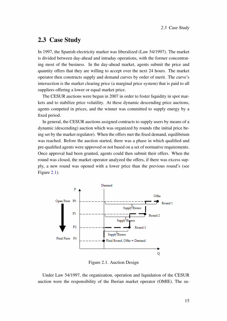
2.3 Case Study
In 1997, the Spanish electricity market was liberalized (Law 54/1997). The marketis divided between day-ahead and intraday operations, with the former concentrat-ing most of the business. In the day-ahead market, agents submit the price andquantity offers that they are willing to accept over the next 24 hours. The marketoperator then constructs supply and demand curves by order of merit. The curve’sintersection is the market clearing price (a marginal price system) that is paid to allsuppliers offering a lower or equal market price.
The CESUR auctions were begun in 2007 in order to foster liquidity in spot mar-kets and to stabilize price volatility. At these dynamic descending price auctions,agents competed in prices, and the winner was committed to supply energy by afixed period.
In general, the CESUR auctions assigned contracts to supply users by means of adynamic (descending) auction which was organized by rounds (the initial price be-ing set by the market regulator). When the offers met the fixed demand, equilibriumwas reached. Before the auction started, there was a phase in which qualified andpre-qualified agents were approved or not based on a set of normative requirements.Once approval had been granted, agents could then submit their offers. When theround was closed, the market operator analyzed the offers, if there was excess sup-ply, a new round was opened with a lower price than the previous round’s (seeFigure 2.1).
Figure 2.1. Auction Design
Under Law 54/1997, the organization, operation and liquidation of the CESURauction were the responsibility of the Iberian market operator (OMIE). The su-
15

2 Predicting Collusive Patterns in Electricity Markets
pervision and validation of the results was the job of the Comisión Nacional deMercados y la Competencia (CNMC), as provided by complementary resolutionsITC/1659/2009 and ITC/1601/2010, and in keeping with principles of transparency,competitiveness and non-discrimination.
A total of twenty-five auctions were held. The last one took place on 19 Decem-ber 2013, in line with the conditions laid down by the Energy Secretary’s resolutionsof 11 June 2010, 20 November 2013 and 11 December 2013 and with the criteriaincluded in complementary resolutions ITC/1601/2010 and ITC/1659/2009. On 20December 2013, however, the CNMC declared the auction void and published areport in which it offered the following reasons: Low eolian production, high un-availability, fall in transactions on the intraday market, increasing demand, risinggeneration costs and a limited interconnection capacity. According to the CNMC,these concerns led the auction participants to behave atypically. Qualified supplierswere lower in number and offers were withdrawn earlier than at other auctions. Theauction was closed in the earliest round ever and, as a result, the resulting equilib-rium price was 7% higher than that on the day-ahead market.
Date AuctionNumber Qualified Round
Numbers Awarded AuctionAmount(MW)
Auction Price(e/MWh)
15/12/2009 10 31 17 26 10,740 40.4023/06/2010 11 33 14 30 4,536 45.2121/09/2010 12 31 14 30 4,392 47.4814/12/2010 13 25 12 22 4,306 49.4222/03/2011 14 23 14 21 4,406 52.1028/06/2011 15 26 17 23 4,288 53.7527/09/2011 16 26 12 25 4,258 58.5320/12/2011 17 28 19 28 4,363 53.4021/03/2012 18 28 14 26 3,451 51.6926/06/2012 19 29 18 25 3,575 57.0925/09/2012 20 28 16 20 3,334 49.7521/12/2012 21 28 18 30 3,345 54.9020/03/2013 22 32 22 29 2,880 46.2725/06/2013 23 34 18 48 3072 49.3024/09/2013 24 37 12 44 2,852 48.7419/12/2013 25 36 7 - 2,833 61.83
Table 2.1. CESUR Auctions. Columns contain date, the auction number, thenumber of qualified suppliers, the number of rounds, the number ofwinning bidders, the auctioned amount and the final auction price.
Table 2.1 shows that the number of qualifiers was similar to previous auctions,however, the final number of rounds was the lowest. In addition, the initial volumeauctioned was lower than previous auctions (2,833 MW). During the first round,suppliers reduced their volume offers by 30.6% (the largest amount ever declinedin a first round). Between 8 to 12 agents decided not to participate in the sec-
16

2.3 Case Study
ond round. The second most important volume reduction was in the sixth round(15.2%), and the equilibrium was finally reached in the seventh round with a priceof 61.83 e/MWh.
One of the characteristics of the CESUR auction was that the information aboutprevious rounds was in aggregated terms, consequently, agents did not have preciseand complete information about supply excess (i.e. they did not know if they werepivotal agents). However, in each round, they knew a range of supply excess. Forexample, in the 25th auction, during the first two rounds, agents knew that therewas a supply excess of 200% (named the blind range). When the third round wasfinished, they knew that the supply excess was around 150-175% (4,250-4,958 MWoffered versus 2,833 auctioned). As a result, qualified suppliers had informationthat the auction was outside the blind range (and, therefore, close to the equilibriumprice). After the fifth round, they already knew that the supply excess was lowerthan 66%.
One of the most striking features of the decision of not applying penalizations wasthat the CNMC, despite finding evidence of abnormal prices and an unconventionalauction, identified only exogenous factors as justification for their stance. Indeed,their understanding was that the low competitive pressure was caused by the neg-ative environment affecting firms, and while they did not validate the results, theydid justify their actions. Subsequently, no penalties were imposed.
The main reasons the CNMC argued were: a low eolian production, high un-availability, increasing demand, and higher generation costs. Figure 2.2 presentsan overview of those factors. Top figure shows eolic source production over totalsources production. During December 2013, 21% of total electricity was producedby eolic sources. The month previous to the 24th auction, eolic sources representedaround 15% of total sources. Furthermore, the eolic production since the first auc-tion was 14% on average.
Additionally, it is not visually clear in the second plot that a large increase indemand could explain this situation. During December 2013 16,699 GW were de-manded, a very similar number to December 2012 (16,267 GW) while still far fromother peak months like April (18,002 GW) or January (17,443 GW).
In terms of power unavailability, 4,961 GW were unavailable in December 2013.The average between July 2007 and November 2013 was 5,369 GW. Moreover, inthe 24th CESUR auction, 8,386 GW were unavailable.
As fossil fuel sources are usually the most expensive technologies, we also showhistorical data about the International Petrol Price per barrel (USD) in Europe andthe International Gas Price (USD/BTU). While the average petrol price during 2012was 111.62 USD per barrel, in December 2013, the average price was 110.75,marginally higher than December 2012 (109.45) and lower than months like Oc-
17

2 Predicting Collusive Patterns in Electricity Markets
tober 2013 and September 2013 (around 111 USD per barrel). The price of gasin December 2013 was slightly higher than the same month in 2012 (4.28 versus3.45 USD/BTU), however, it was not excessively different from many other monthsduring the period analysis.
Figure 2.2. Main Factors Argued by the CNMC. Plots contain wind productionover total production, total demand (GWh), unavailable power (GW),international petrol price (USD per barrel) and international gas price
(USD/BTU).
On one hand, it is true that there was a lower volume auctioned and that therewere higher declined volumes, on the other hand, it is hard to explain that there wereexogenous factors that could explain this situation. However, it is still not clear ifagents could extract information (due to the auction design) that may contribute totacit collusion and if the output in this particular auction was an isolated case or waspart of a repeated hidden action.
As was pointed out by Fabra and Fabra Utray (2012), Electric companies hadseveral incentives to keep a higher CESUR price. Besides risk premiums to covervolatility in the spot market, there were also payments and discounts tied to theenergy sell. The question is then: if collusion exists, which mechanisms throughsuppliers could have affected the CESUR price?
First, as we mentioned before, they could take off their bids, i.e. reduce compet-itive pressure. Second, they could alter expectations by artificially increasing dailymarket prices the days previous to the auctions. In this chapter, and as data aboutbidder identities or transactions on previous auctions is not public, we focus on thesecond mechanism.
18

2.3 Case Study
2.3.1 Forward Premium2
The ex-post forward premium is defined as the difference between the auction priceand the spot price during the delivery period. Competitive auctions imply ex-postforward premiums close to zero.
Table 2.2 compares prices for the auctions delivered by the market operator. Theaverage ex-post forward premium during this period was 9.42%3. In only 3 outof 19 auctions, ex-post premium was negative. The same conclusion is stated byPeña and Rodriguez (2018). They do the same analysis considering the total num-ber of CESUR auctions, finding an ex-post forward premium average of 7.22%.This translated into euros represented around 1,000 million overpaid cost for theconsumers.
Date AuctionNumber
Auction Pricee/MWh
Daily Price(e/MWh)
Ex-Post ForwardPremium (e/MWh)
Ex-Post ForwardPremium (%)
Petroleum PriceVariation (%)
Gas PriceVariation (%)
25/09/2008 6 72.48 64.65 7.83 10.80 % -52.2 % -23.9 %16/12/2008 7 56.47 43.1 13.37 23.68 % -18.7 % -29.1 %26/03/2009 8 36.84 36.99 -0.15 -0.41 % 32.1 % -15.7 %25/06/2009 9 44.54 33.96 10.58 23.76 % 20.6 % 3.4 %15/12/2009 10 40.40 39.96 0.44 1.10 % 8.7 % 21.9 %23/06/2010 11 45.21 44.07 1.14 2.51 % -0.2 % -11.8 %21/09/2010 12 47.48 43.33 4.15 8.74 % 9.3 % -8.7 %14/12/2010 13 49.42 45.22 4.20 8.50 % 21.0 % 9.5 %22/03/2011 14 52.10 48.12 3.98 7.64 % 15.5 % 3.1 %28/06/2011 15 53.75 54.23 -0.48 -0.89 % -3.4 % -6.7 %27/09/2011 16 58.53 52.01 6.52 11.14 % -3.5 % -14.7 %20/12/2011 17 53.40 50.64 2.76 5.17 % 8.3 % -27.7 %21/03/2012 18 51.69 46.07 5.62 10.87 % -8.6 % -5.3 %26/06/2012 19 57.09 49.09 8.00 14.02 % 1.2 % 22.5 %25/09/2012 20 49.75 43.16 6.59 13.25 % 0.4 % 20.8 %21/12/2012 21 54.90 40.34 14.56 26.52 % 2.2 % -1.6 %20/03/2013 22 46.27 34.26 12.01 25.96 % -8.8 % 16.9 %25/06/2013 23 49.30 49.81 -0.51 -1.03 % 7.5 % -13.0 %24/09/2013 24 48.74 54.73 -5.99 -12.28 % -1.7 % 2.8 %
Table 2.2. Auction Prices Compared to Daily Prices
A reason usually argued for why long-term contracts auctions may result in pos-itive ex-post forward premiums is that bidders are expecting a risk premium. Asthey are taking risk by selling long-term fixed contracts, they should be able tocover their generation costs. This is mainly relevant for fossil generators that aretied to international price fluctuations. However, as we will see later, Spain has quitea diversified energy source structure where fossil fuels are not the main resource.In addition, columns in Table 2.2 contain petroleum and gas price variations duringdelivery periods. If the risk premium argument would be true, negative price vari-ations should be related to non-positive ex-post forward premiums, and vice versa,although a majority of periods with negative variations have had positive premiums.
2We thank an anonymous referee for this suggestion.3The ex-post forward premium is calculated as PCESUR−PSpot
PSpot
19

2 Predicting Collusive Patterns in Electricity Markets
2.3.2 Sector Concentration
Since 1997, privatization and liberalization processes in Spain’s electricity genera-tion market have tended to concentrate the sector. At the start of the auctions, twoenterprises accounted for 64% of the country’s generation capacity (Agosti et al.,2007). Table 2.3 summarizes the shares of net power installed 4.
Firm Net Power (MW) Shares
Iberdrola Generación S.A. 20,017 34.8%Endesa Generación S.A. 16,614 28.9%Unión Fenosa Generación S.A. 5,959 10.4%Gas Natural SDG, S.A. 2,791 4.9%Hidroeléctrica del Cantábrico, S.A. 2,428 4.2%Enel Viesgo Generación, S.L. 2,259 3.9%Others 7,408 12.9%Total MW 57,476
Table 2.3. Installed Capacity by firms
Source: Agosti et al. (2007)
These two firms had a pivotal index rate5 below 110% for more than 5% of thetime, the threshold for considering the existence of a power market according tothe European Commission. Moreover, interconnection with Europe was limited(excluding Portugal and Morocco). More particularly, Spain was under the 10%interconnection threshold recommended by the European Commission. Could thesefactors have contributed to price collusion?
It is therefore not surprising that after the 25th auction, 80% of the total auctionedvolume was distributed between two firms: Iberdrola and Endesa6 (see Table 2.4).
In addition to the inherent characteristics of the Spanish market, other factorscould have affected prices. For instance, the external volatility may have adverselyaffected the firms’ price decisions. According to this hypothesis, the design of theauctions (a fixed price during a fixed period) incentivized firms to charge a riskbonus which was also transferred to the daily market.
Determining whether prices are driven by external shocks is important for anysubsequent impact analysis. Here, we propose exploiting the introduction of theCESUR auction across time and the market to identify the causal effect of introduc-ing fixed long-term tariffs on prices using a triple difference-in-difference approach.
4This excludes generators with a power below 50 MW.5The pivotal index rate seeks to show whether it is possible to supply the prevalent demand
without a particular supplier.6Union Fenosa was acquired by Gas Natural in July 2008.
20

2.4 Theoretical Model
Auction Price (e/MWh) 61.83Auction Amount (MW) 2,833Iberdrola Generación S.A. 924Endesa Generación S.A. 1,336Gas Natural SDG, S.A. 480Others 93
Table 2.4. Winning Bidders - Auction 25th
2.3.3 Nord Pool
Nord Pool AS is the electrical energy market operating in Norway, Denmark, Swe-den, Finland, Estonia, Latvia, Lithuania, Germany and the UK (but, note, that dur-ing the period analyzed Germany and the UK were not yet members and Lithuaniadid not join until June 2013). Here, we use the day-ahead Nord Pool market as acontrol group for the Spanish market given that the two markets were not relatedduring the period analyzed.
As mentioned above, the CESUR auction was operational between 2007 and2013. However, we should highlight that data for the control group are only avail-able from 2013 onwards. Therefore, our estimations here refer to the period of daysbetween 2013 and 2014, where 2013 is considered as a treated year (during whichthree auctions were held) and 2014 as a control year.
Table 2.5 shows total production (MWh) by country in the period analyzed. Ascan be seen, Norway and Sweden produced more than 70% of Nord Pool’s totalproduction.
Year Norway Sweden Finland Denmark Latvia Lithuania Spain2013 133,385,250 147,770,389 65,952,798 32,491,906 2,795,241 3,543,888 186,569,8062014 141,158,884 149,710,633 64,587,200 30,648,162 4,903,420 2,959,173 170,399,215Shares 35% 38% 17% 8% 1% 1% -
Table 2.5. Total Production (MWh) by Country
Table 2.6 reports the sources of electricity generation by country. While Spainhas quite a homogeneous structure, Nord Pool presents, overall, a highly depen-dent generation structure. For instance, 97% of Norwegian and 48% of Swedishproduction are extremely dependent on hydraulic sources.
2.4 Theoretical Model
We construct a very simple model to illustrate the possible implications of introduc-ing fixed-price contract obligations. We consider two symmetric firms which sell
21

2 Predicting Collusive Patterns in Electricity Markets
Source Norway Sweden Finland Denmark SpainEolic 1.08% 4.40% 0.74% 26.28% 21.10%Other Renewables 0.00% 6.69% 15.36% 31.89% 20.00%Fossil Fuels 2.30% 2.85% 25.26% 41.84% 23.60%Nuclear 0.00% 37.92% 32.64% 0.00% 20.40%Hydraulic 96.62% 48.14% 24.67% 0.00% 11.80%Others 0.00% 0.00% 1.33% 0.00% 3.10%
Table 2.6. Share of Electricity Generation by Country
a homogeneous good with constant marginal cost c. We also assume that they arerisk neutral. The firms offer q which is covered perfectly by the demand.
We consider two auction formats: a uniform-price auction (the price received isthe market price) and a discriminatory-price auction (the price received is equal toits own bid).
We have two markets: a daily market where the price mechanism is a uniform-price auction and a discriminatory-price auction which works every 2t periods. Thetiming of the game is represented as follows: Each firm simultaneously and inde-pendently submits a bid in the daily market specifying the minimum price at whichit is willing to supply. As demand perfectly matched supply, both firms dispatchtheir total production. On the other market, the firms submit different bids bsi , andthe lower bidder is the only firm that can deliver at that price. However, the quantitythat is produced in this market (a fixed quantity q set by the auctioneer) cannot bedelivered in the daily market.
Formally, the quantity produced by the firm i (i = 1,2) in the daily market isgiven by:
(2.1)qdi =
qi − q bsi ≤ bsj
qi bsi > bsj
The lowest accepted bid bd in the auction is referred to as the market price P , andcan be expressed as:
(2.2)P =
bdj (qj) bdj ≤ bdi
bdi (qi) bdj > bdi
In the secondary market (the discriminatory-price auction) the price is set by thelowest auction, i.e., bs =min(bsi , b
sj), and the quantity produced is:
(2.3)qsi =
q bsi ≤ bsj
0 bsi > bsj
22

2.4 Theoretical Model
At the end of each stage, the two firms receive their profits. The auctioneerannounces the market price in the daily market and which firm is to deliver in thesecondary market (if it is a 2t period).
We explore an infinitely repeated game, with a strategy profile (Si,Sj) and thepayoff for each firm is the sum of their discounted profits, where ρ ∈ (0,1) is thediscount rate.
If the firms collude they will set a price P in the daily market and a price bs inthe secondary market. However, as the winning firm in the secondary market is notable to sell q in the daily market, it should earn at least bs ≥ P . The discountedfuture benefits if the firms i collude are:
πCi = (P − c)qdi (1 +ρ+ρ2. . . ) + (bs− c)qsi (ρ2 +ρ4 + . . . )
When the firms do not collude, they compete in the daily market and set a com-petitive price b in the secondary market. However, the firms set a b bid equal at leastto the daily market price (i.e., b≥P ). If the firms i do not collude, future discountedbenefits can be expressed as:
πNCi = (P − c)qdi (1 +ρ+ρ2. . . ) + (b− c)qsi (ρ2 +ρ4. . . )
We consider trigger strategies where the firms sustain a collusion price in the setP , b in each period if and only if the firms do not deviate in previous periods, i.e.,the collusion price path is an equilibrium of the perfect subgame equilibrium if andonly if:
πC(t,ρ)≥ πNC(t,ρ)∀t
Formally,
πC −πNC =1
1−ρ(P −P )qdi +
∞
∑t=1
ρ2t[b− b]≥ 0
The left side of the equation corresponds to the benefits of colluding in the dailymarket, while the right side corresponds to the benefits of colluding in the secondarymarket. If the firms do not collude in the secondary market, they can deviate in thesecondary market and set a bid b− ε and obtain all the profits. This means thatfirms will compete until they obtain a price P , which guarantees them at least thesame profits as in the daily market. Therefore, the low boundary bid has to be b≥P .Likewise, for both firms to make a profit, and not to deviate in the secondary market,one firm has to profit from losing the secondary market auction, i.e., obtain profitsin the daily market, that is, P ≥ P .
23

2 Predicting Collusive Patterns in Electricity Markets
Proposition 1 Exists ρ ∈ (0,1) such that the set price {bi, bj , P ,P}∞t=1 is a sus-tainable equilibrium of the perfect subgame if and only if ρ ∈ (ρ,1).
What is interesting about the results is that the fixed-price contract (the secondarymarket auction) introduces an additional effect in the collusive pattern. Withoutthis, the incentives to collude would be the same as those not to collude, becausethere would be no motivation to raise prices in the daily market. Yet, with theintroduction of the secondary market, both firms have to set higher prices to ensurethat the auction loser obtains at least the same benefits as those obtained by thewinner. To guarantee that the loser obtains the same benefits for the q ratio, thefirms have to set a price P at least higher than that of the bids (bsi , b
sj).
Proposition 2 Consider ε, an exogenous positive price shock which affects thedaily market price immediately after the second market auction is finished. Then,the subgame equilibrium is one where b > b∗, where b∗ is the price obtained in thesecondary market when there are no shock prices.
To prove Proposition 2, we assume an ε > 0 which affects spot market pricesimmediately after the second market auction is held, with probability p. To simplify,we assume one of the firms always loses the auction and the other always wins. Wecan express the future discounted benefits of the firm that wins the auctions as:
πW = (P−c)(qW− q)(1+ρ+ρ2. . . )+(b−c)q(ρ2+ρ4. . . )+pε(ρ2+ρ4. . . )(qW− q)
And the future discounted benefits of the firm that loses as:
πL = (P − c)qL(1 +ρ+ρ2. . . ) +pε(ρ2 +ρ4. . . )qL
For colluding firms, the price path is an equilibrium of the perfect subgame equi-librium if and only if:
πW (t,ρ) = πL(t,ρ) ∀t
Then, we can rearrange as:
24

2.5 Methodology
πW −πL = (P − c)(qW − qL)1
1−ρ+pε
∞
∑t=1
ρ2t(qW − qL)−
q
[(P − c) 1
1−ρ+pε
∞
∑t=1
δ2t
]+∞
∑t=1
ρ2t(b− c) = 0
To simplify the results (which does not affect the general conclusions), we as-sume that both firms produce the same quantity (qW = qL):
−(P − c)q 1
1−ρ−pε
2t
∑t=1
q+∞
∑t=1
ρ2t(b− c)q = 0
The first left-hand term is the opportunity cost of the winning firm not sellingq in the daily market. The second term is the opportunity cost of its not derivingthe positive shock in the quantities sold q. Finally, the third term is the profit madefrom winning the auction in the secondary market. Without a shock, the secondterm is null, and therefore, the profits of the secondary market auction derived fromProposition 1 have only to cover the opportunity cost of not selling in the dailymarket. However, in this new equilibrium, to be sustainable (with ρ, c and q fixed),i.e. to keep this equality, b must be higher than b∗. Also P is higher than theequilibrium price without a positive shock.
A number of preliminary conclusions can be derived from these two propositions.Artificially applying fixed-price auctions of this kind creates incentives to increaseprices in the daily market. As seen, this effect could emerge for two reasons: First,repeated auctions trigger collusion because of their inherent format and because ofthe structural collusion present in the daily market (Proposition 1). Second, un-certainty in the daily market pushes firms to follow the expected price path in thesecondary market (Proposition 2). In conclusion, for whatever reason, what trig-gers collusion is not the introduction of the regulation per se, but the actual designof that mechanism. In the following section, we present the empirical methodologyto measure the size of this effect.
2.5 Methodology
In the following sections we describe our methodology to evaluate the impact ofintroducing fixed long-term tariffs on prices in the Spanish case. We are interestedin two aspects: a) identifying abnormal patterns in the daily market due to the in-troduction of the CESUR auction, b) measuring the economic impact in terms of
25

2 Predicting Collusive Patterns in Electricity Markets
higher daily prices. As we explained previously, electric companies had incentivesto get higher CESUR prices. The mechanism we are focusing on is one in whichfirms could be influencing parallel markets to inflate CESUR price expectations.Therefore, we divide our analysis as follows: in Section 2.5.1, we present an AR-MAX model combined with Instrumental Variables (IV) to identify if there wereabnormal behaviors on daily prices during the previous days to the auctions, i.e.find evidence that firms were inflating expectations in the daily market to get betterprices in the CESUR auction. Once we identify abnormal price behavior we pro-pose in 2.5.2 a triple differences model (DDD) to measure the economic impact onenergy prices.
2.5.1 Price Dynamic in Electrical Markets
The dependent variable in our analysis is the logarithm of the daily price. Thedatabase includes daily data on prices and production obtained from OMIE andNord Pool during the period 2013-2014. The weather condition variables are fromNational Centers for Environmental Information. We also include the InternationalPetrol Price in Europe, the International Price of Gas (USD/BTU) and Spain’s RiskPremium relative to Germany. Finally, three auctions were held in 2013: 20 March2013, 25 June 2013 and 24 December 2013.
If there were abnormal price phases during the period analyzed (whether resultingfrom collusion or not), the question is how these periods can be best defined. Ourmain objective is to understand when the dynamics of prices in the Spanish marketand that of prices in the Nord Pool market present a different pattern. To do so,we add a dummy variable (IP - Investigation Period) before, during and after theauctions that is equal to one for each specific time window. We test our results forthe three auctions held in 2013. In addition, given that the auctions were canceledin 2014, we can use this year as a falsification test.
As we are modeling electricity prices that are simultaneously set by supply anddemand, several questions have to be addressed before we continue. Ordinary leastsquare (OLS) estimates are based on the assumption that all independent variablesare uncorrelated with the error term (exogeneity assumption). When this occurs, theconditional expected error term is equal to zero for each observation, which impliesthat the regressors are orthogonal to the error term.
However, we might expect the error term to be correlated with quantity, giventhat quantity depends on other factors (omitted bias). Additionally, the prices andquantities observed reflect equilibrium sets between supply and demand, i.e. theyare determined simultaneously and the estimation may therefore be affected by thesimultaneity bias (Angrist and Krueger, 2001). As such, we cannot infer if changes
26

2.5 Methodology
in price are due to supply or demand shifts.In addition, the nature of the product (perfect synchronization without storage
capacity) causes high price volatility. This means the price is highly affected byits dynamics which inherits some of the distinctive features of demand, such asseasonality effects (Fezzi, 2007). Moreover, supply and demand must be constantlybalanced, but as shocks cannot be smoothed, they are immediately transferred toprices.
All these issues are crucial elements to take into account when estimating elec-tricity price dynamics: Simultaneity bias, non-stationarity, non-normality and serialcorrelation should each be carefully examined.
Formally, we initially define an autoregressive moving average model with ex-ogenous input terms (ARMAX) that can be expressed as:
yt = βXt+γIPt+α1QIV Spaint +α2Q
IV NPoolt +
p
∑i=1
φiyt−i+m
∑j=1
θjµt−j +µt (2.4)
where yt is the dependent variable and is equal to log(PSpain/PNPool). PSpainis the daily arithmetic average price of the spot market in Spain, and PNPool is thedaily arithmetic average price of the spot market in Nord Pool. IP is the indicatorwhich reflects switching phases and QIVt is the quantity production of each market(Spain, Nord Pool expressed in logarithms), both quantities being instrumental vari-ables (see section Appendix A: Instrumental Variables Tests). X is the vector thatrepresents explanatory variables and the model orders p, m refer to p autoregressiveand m moving average terms.
Following the practical approach developed by Box et al. (2015) to select anappropriate ARMA model with the corresponding extensions applied to ARMAXmodels (Andrews et al., 2013) – see Appendix B: ARMAX Model-Building Process– we choose our main exogenous candidate variables which are reported in Table2.7. All the variables are expressed in MWh (as logarithms). Dummy Null Priceare two atypical days in April 2013, when prices in Spain were equal to zero.
2.5.2 Identification and Estimation Methods
Our second objective is to identify the average effect of mandated auctions on pricesin the market and the year in which regulations of this type were introduced. Specif-ically, we are interested in comparing prices the days before mandated auctionswere introduced with the counterfactual, i.e. prices in a different market on the
27

2 Predicting Collusive Patterns in Electricity Markets
Exogeneous-Variables CandidatesNord Pool ProductionSpain ProductionPortugal ProductionSpain Production Lag-1Spain ImportsDummy Null Price
Table 2.7. Stepwise Regression Variable Candidates
same days.A major concern is that the country that chose to introduce the regulation is likely
to be different from the country that did not and that such differences may be cor-related with prices. In principle, many of the unobservable characteristics that mayconfound identification are those that vary across markets but are fixed over time.A widely used method for controlling time-invariant unobserved characteristics andunexpected variations is to use panel data and estimate difference-in-differencesmodels.
A difference-in-differences estimation (Angrist and Krueger, 1992; Card andKrueger, 1994; Meyer, 1995 are the precursors) measures the impact of a policychange on an outcome variable by removing the effects of time and place. Whenthe outcome depends on the policy, time, place or other variables, we can addition-ally reduce the bias in the estimated effect by using a triple difference-in-differences(Berck and Villas-Boas, 2016). The goal of this empirical study is to capture theeffect of fixed price long-term auctions held in 2013 (experimental year) and whichimpacted Spain (treatment group). Identifying this effect implies controlling at thesame time for any systemic shocks that could have disturbed the electricity marketoutcomes of the treatment group in the experimental year. Higher prices in Spainwhen the regulations are in place can then be considered as the net effect of regula-tion. To control for economic changes that are unrelated to the program, we use amarket (Nord Pool) which was unaffected by the regulation.
The overall difference-in-differences can be written as:
DD = E[(Y Tt −Y Tt−1)|IPt = 1]−E[(Y Ct −Y Ct−1)|IPt = 0]
where Y Tt is the treated group in time t (Spain, 70 days before each auction in2013), Y Ct is the control group in time t (Nord Pool, 70 days before each auction in2013) and IPt is an indicator of the policy effect.
Recall that, in 2014, the law governing CESUR auctions was lifted; thus, we canuse 2014 as an additional control by using triple differences (DDD):
28

2.6 Results
DDD = E[(Y Tt −Y Tt−1)|IPt = 1]−E[(Y Ct −Y Ct−1)|IPt = 0]
−E[(Y Tt+2−Y Tt+1)|IPt+2 = 1]−E[(Y Ct+2−Y Ct+1)|IPt+2 = 0]
where Y Tt+2 is the treated group in time t+2 (Spain, 70 days before the same daythe auctions where celebrated but in 2014), and Y Ct+2 is the control group in timet+ 2 (Nord Pool, 70 days before the same day the auctions were held but in 2014).
The left part of the equation expresses two concepts: first, the difference betweendaily prices of the treatment and control group 70 before each auction (Y Tt −Y Ct ).This term should be positive if mandated auctions introduce incentives to increaseprices. Second, the difference between daily prices of the treatment and controlgroup during previous periods considered as untreated (Y Tt−1−Y Ct−1). This controlfor unobservables that affect differences in daily prices and are constant over time.
The right-part of the equation introduces another two concepts: first, the differ-ence between treatment and control group in the non-experimental year (Y Tt+2−Y Ct+2).It controls market individual differences that may affect prices in days inwhich auctions would have been applied (in 2014) if they were not cancelled. Sec-ond, (Y Tt+1−Y Ct+1) controls for market individual differences that affect prices dur-ing the same days that auctions would have not been applied. Overall, it controlsomitted variables that cause differences in daily prices to change over the period.
This can be simplified as:
DDD =DD2013−DD2014
DDD will consistently identify the effect of the policy if two conditions hold:First, the differences in prices in 2013 are related to the auctions, i.e., DD2013 > 0.Second, there are no differences in prices in the counterfactual year, i.e., DD2014 =
0.
2.6 Results
In this section, the model results are analyzed. As mentioned before, we first iden-tify abnormal periods in the daily market. Second, we present our identificationstrategy and, third, we measure the average effect of mandated auctions on prices.
29

2 Predicting Collusive Patterns in Electricity Markets
2.6.1 Windows Choice
We present the equation (1) estimation results in Table 2.8. We analyze whetherdaily prices are consistent with the hypothesis of expected inflation near auctiondates. Our focus is on the Investigation Period variable (IP), which is a dummy thattakes one during days surrounding auctions. We test whether there are significantdifferences between Spanish daily prices and Nord Pool daily prices. Additionally,we validate our analysis conducting the same experiment during a year withoutauctions.
The table highlights that, during 2013, there are significant, positive and per-sistent price differences between 0 and 70 days before the CESUR auctions. Thedifferences are between the daily average Spanish prices and the daily average ofthe Nord Pool market. Those differences oscillate between 68% and 222%. Afterthat, we find no conclusive evidence of increasing prices.
We also report estimations during 2014 of the Investigation Period variable. Aswe mentioned earlier, auctions were cancelled after December 2013. Therefore,we would expect no relation between the Investigation Period variable and dailyprices. The results from the simulation in 2014 are also displayed in Table 2.8. Asexpected, we do not find any evidence of price differences, which initially supportsthe hypothesis that regulation negatively affected consumers.
Days -90 -85 -80 -75 -70 -65 -60 -55 -50 -45 -30 -25 -20 -15IP 2013 -0.07 0.31 0.35 0.37 0.84*** 0.83*** 0.52** 0.72*** 0.65** 1.17*** 0.85*** 0.62** 0.63*** 0.86***IP 2014 0.20 -0.18 -0.05 0.10 -0.05 0.08 -0.02 0.07 0.32 -0.19 -0.08 -0.04 -0.05 0.02
Days -10 -7 -5 -3 0 3 5 7 10 15 20 25 30 45IP 2013 0.34 0.54** 0.92*** 0.70*** 0.79*** -0.99*** -0.41 1.11*** 0.56* 0.71** 0.14 -0.34 -0.33 -0.15IP 2014 0.22 -0.05 -0.03 0.22 -0.02 0.03 0.06 0.23 -0.01 -0.20 0.09 0.12 0.06 0.28*
Table 2.8. Window Time Choice
To validate that 70 days before each auction is representative of abnormal be-havior in daily prices, we propose a long short-term memory network model (seeAppendix C for a complete specification of the model). Here, our main concern isto demonstrate that the abnormal period of collusion chosen is in fact correct. To doso, we employ a deep learning model operating as an outlier detection model. Theadvantage of models of this type is that they are well suited to predicting patterns.Although we cannot assess the marginal impact of the variables, we can use thesemodels to verify if our switching regression pivotal variable is correctly defined.
In Figure 2.3 we illustrate the results for the normal observations. The upperpanel of the figure plots the true values, predicted values and error values, while thelower panel shows the logarithm of the probability density function of the error testusing the mean and the covariance of the training error vector. If values are belowthe “normal” threshold, they are considered abnormalities.
30

2.6 Results
Figure 2.3. Normal Data Test
In this particular case, when testing the normal data for 2013, only five days wereconsidered to be abnormal. However, when we focus on the 70 day-period beforethe CESUR auctions (see Figure 2.4), almost every day is abnormal. Specifically,we obtain a Precision of 100% and a Recall of 81%7.
Figure 2.4. Abnormal Data Test
Therefore, empirical evidence supports the hypothesis of inflating prices the dayprevious to the auction. The introduction of long-term tariff auctions is related tolarge price differences between Spanish and Nord Pool markets. Thus, our choice
7Precision = True Negatives / (True Negatives + False Positives), Recall = True Positives / (TruePositives + False Negatives)
31

2 Predicting Collusive Patterns in Electricity Markets
of the 70-day time period prior to the CESUR auctions as our main candidate seemsto be accurate. Indeed, during this period, we captured recurrent abnormal patternsin energy prices.Hereinafter, therefore, we propose using the dummy 70 days beforea CESUR auction as our collusive or abnormal phase variable. We now turn to thequestion of what the net impact on prices when long-term tariffs were introduced.To shed light on this point, we compute triple differences between Spanish and NordPool markets and between 2013 and 2014.
2.6.2 Identification Strategy
Although market regulators introduce mandated auctions to foster competition andprovide energy at a competitive price, we have found that the particular character-istics of electricity markets (high concentration and high volatility) may produceundesired effects on daily markets. In this section, we study to what extent dailyprices were affected by the introduction of regulation.
To measure the effect on the actual price increase due to the CESUR auctions,it would be necessary to observe how the electric market behaves in two differentstates: one in which the regulation was applied, and one in which it was neverapplied. The increase in prices when the auction is held compared to when it is notwould therefore be the actual effect of the regulation. As it is impossible to observethe same market in a counterfactual state, the best approach is to use “comparables”.Thus, it is necessary to create counterfactuals that are nearly identical and whichwill enable us to control for additional sources of omitted variable bias.
However, it is almost impossible to have two virtually equal markets. Here iswhere a triple differences estimation is useful. A difference-in-differences modelcontrols for omitted variables that could affect differences in daily prices betweenthe Spanish market and the Nord Pool market, and that are constant over time. Themain advantage of using a DDD model is that, in addition to controlling for thosefactors, we will also be able to control for omitted variables that affect differencesin daily prices over time for each of those markets. This will help us get betterunbiased estimates of the true effect of mandated auctions.
Table 2.9 summarizes individuals’ statistics in the treatment and the control groupand in experimental and non-experimental years. The Difference column showsdifference in means tests. In Spain, there were almost no significant differences inthe source production structure. However, there is a decrease in the fossil production(explained by a decrease in combined cycle power production) that can be related tooil and gas price variations (which are also significant). Therefore, it is important toinclude them as control variables. Eolic production also has a significant difference,but we believe that this difference is quite small and should not bias the results.
32
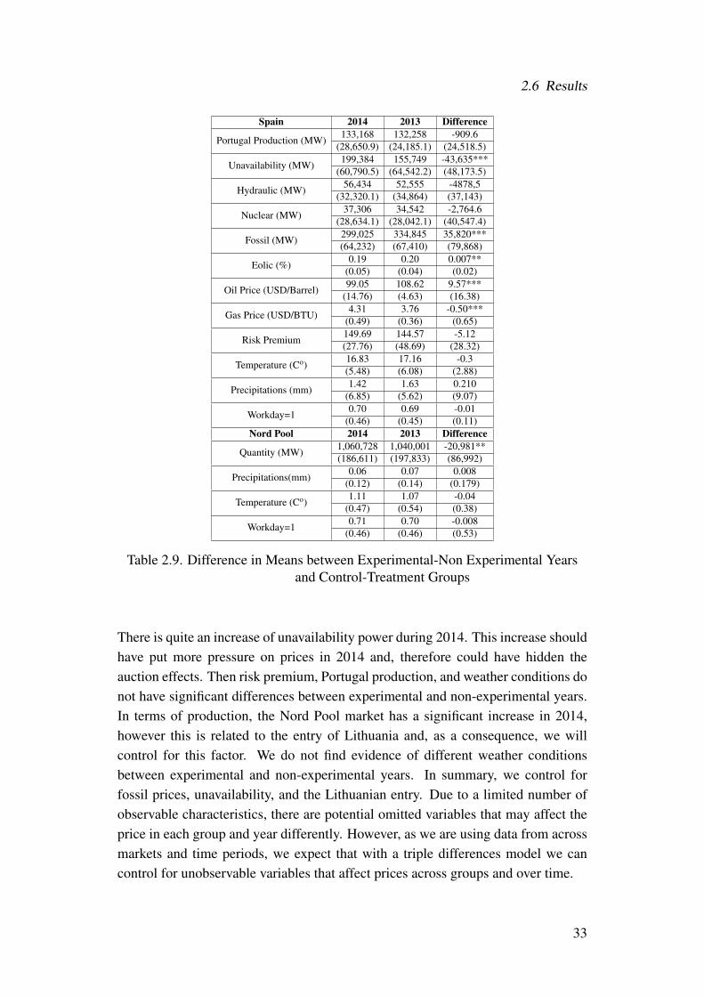
2.6 Results
Spain 2014 2013 Difference
Portugal Production (MW)133,168 132,258 -909.6
(28,650.9) (24,185.1) (24,518.5)
Unavailability (MW)199,384 155,749 -43,635***
(60,790.5) (64,542.2) (48,173.5)
Hydraulic (MW)56,434 52,555 -4878,5
(32,320.1) (34,864) (37,143)
Nuclear (MW)37,306 34,542 -2,764.6
(28,634.1) (28,042.1) (40,547.4)
Fossil (MW)299,025 334,845 35,820***(64,232) (67,410) (79,868)
Eolic (%)0.19 0.20 0.007**
(0.05) (0.04) (0.02)
Oil Price (USD/Barrel)99.05 108.62 9.57***
(14.76) (4.63) (16.38)
Gas Price (USD/BTU)4.31 3.76 -0.50***
(0.49) (0.36) (0.65)
Risk Premium149.69 144.57 -5.12(27.76) (48.69) (28.32)
Temperature (Co)16.83 17.16 -0.3(5.48) (6.08) (2.88)
Precipitations (mm)1.42 1.63 0.210
(6.85) (5.62) (9.07)
Workday=10.70 0.69 -0.01
(0.46) (0.45) (0.11)Nord Pool 2014 2013 Difference
Quantity (MW)1,060,728 1,040,001 -20,981**(186,611) (197,833) (86,992)
Precipitations(mm)0.06 0.07 0.008
(0.12) (0.14) (0.179)
Temperature (Co)1.11 1.07 -0.04
(0.47) (0.54) (0.38)
Workday=10.71 0.70 -0.008
(0.46) (0.46) (0.53)
Table 2.9. Difference in Means between Experimental-Non Experimental Yearsand Control-Treatment Groups
There is quite an increase of unavailability power during 2014. This increase shouldhave put more pressure on prices in 2014 and, therefore could have hidden theauction effects. Then risk premium, Portugal production, and weather conditions donot have significant differences between experimental and non-experimental years.In terms of production, the Nord Pool market has a significant increase in 2014,however this is related to the entry of Lithuania and, as a consequence, we willcontrol for this factor. We do not find evidence of different weather conditionsbetween experimental and non-experimental years. In summary, we control forfossil prices, unavailability, and the Lithuanian entry. Due to a limited number ofobservable characteristics, there are potential omitted variables that may affect theprice in each group and year differently. However, as we are using data from acrossmarkets and time periods, we expect that with a triple differences model we cancontrol for unobservable variables that affect prices across groups and over time.
33

2 Predicting Collusive Patterns in Electricity Markets
The identifying assumption of the DDD (Gruber, 1994) only requires that therebe no shock that affects the relative outcomes of the treatment group in the samecountry-year as the regulation.
In short, our treatment group is Spain while our control group is Nord Pool (i.e.,the market unaffected by the policy). However, the counterfactuals are also consid-ered between experimental and non-experimental years.
Therefore, we transform our data-set to panel data and adopt a triple difference-in-differences approach. By comparing changes, we control for observed and un-observed time-invariant market characteristics that might be correlated with the in-troduction of the policy decision as well as with prices.
Formally, the DDD model can be specified as:
Pijt = β1xijt+β2IPt+β3ρj +β4Ti+β5ρjIPt+
β6IPtTi+β7ρjTi+β8ρjIPtTi+ εijt (2.5)
where Pijt is the logarithm of the price in the market i (Spain, Nord Pool), in theexperimental year j (2013, 2014) on day t. IPt is an indicator variable that takesa value of one 70 days before the auctions and zero otherwise. Ti is a fixed effectunique to market i and ρj is a time effect common to both markets in year j. xijt is avector of covariates that vary across markets and time. Among the control variables,we maintain the autoregressive terms and the instrumental variables to control forthe biases discussed above (see Bertrand et al., 2004, for a detailed discussion).
β1 are several control variables that are unique for each market and causes dif-ferences in daily prices (We include Oil Price, Gas Price, Power Unavailability,Autoregressive Terms, a production variable estimated through instrumented vari-ables, a dummy that takes into account the entrance of Lithuania to the Nord Poolmarket and a Workday variable). β2 controls for any change that affects daily pricesand is changing over time in both experimental and non-experimental years. β4controls for anything that affects daily prices, that differs between markets, that dif-fers between experimental/non-experimental years and that is constant within theyears. β5 controls for everything that changes over time in the experimental year.β6 controls for any factors that affect daily prices across time for both markets butare constant across experimental and non-experimental years. β7 controls for dif-ferences between Spanish and Nord Pool markets in the experimental year and areconstant over time.
The third-level interaction β8 captures the DDD estimation, i.e. the variationin prices specific to the treatment market in the experimental year, 70 days before
34

2.6 Results
the auctions (relative to the control market, non-experimental year and untreatedperiod). The key identifying assumption for this interpretation is that the changein prices is an unbiased estimate of the counterfactual. While we cannot directlytest this assumption, we can test the hypothesis of parallel trends in the control andtreatment markets during pre-intervention periods and during the non-experimentalyear. If the trends are the same in the pre-intervention periods, then we would expectthe same pattern in the post-intervention period in both markets.
Further insights into this behavior are provided in Figure 2.5 where auctions num-ber 24 and 25 are depicted. Note that we only have information from January 2013onwards and so we cannot test the parallel trend assumption prior to the first auc-tion. We use the Hodrick-Prescott filter to remove the cyclical component (Hodrickand Prescott, 1997). Treatment days lie between the dotted and solid lines. Beforethe dotted lines, we would expect to find parallel trends, and thereafter, divergenttrends. As can be seen, in the pre-intervention period, prices in both markets presenta similar pattern. However, immediately after treatment, while the pattern of pricesin the Nord Pool market did not change, the prices in the Spanish market increased.
(a) Auction Number 24
(b) Auction Number 25
Figure 2.5. Parallel Trend
35

2 Predicting Collusive Patterns in Electricity Markets
We formally test that the pre-intervention time trends and the non-experimentalyear for both the control and treatment groups are not different in the absence ofregulation. This requires that the difference between the two markets is constantover time. In this model, we have multiple treated periods which makes it difficultto provide a simple visual inspection. One way to test the assumption of paralleltrends is to evaluate the leads (LE) and lags (LA) of the treatment effect (Pischke,2005). Thus, instead of a single treatment effect, we include m leads and q lags:
Pijt = β1xijt+β2IPt+β3ρj +β4Ti+β5ρjIPt+
β6IPtTi+β7ρjTi+q
∑t=−m
αtγjIPt ∗Ti+ εijt (2.6)
where αt is the coefficient of the tth lead or lag. In Figure 2.6, we illustratewhat it is we are looking for. Thus, in 2013, we would expect the treatment effectto show a divergent trend (α1, α2, α3 are positive). On the other hand, before thetreatment effect we would expect to find a parallel trend (α−1, α−2, α−3 are zero).However, in 2014, we would expect to find a parallel trend across the whole periodand, therefore, all γ coefficients should be zero.
(a) Year 2013
(b) Year 2014
Figure 2.6. Schematic Representation of Leads and Lags
Our results are reported in Table 2.10: The key assumption of parallel trendsbefore the treatment effect is fulfilled. Again, we should stress that we only haveinformation from January 2013 onwards and we cannot, therefore, test the paralleltrend effect prior to the first auction.
36

2.6 Results
Parallel Trends coef
LA_trend_3_2013 -
LE_trend_3_20130.2161**
(0.11)
LA_trend_2_2013-0.0586(0.084)
LE_trend_2_20130.1699***
(0.046)
LA_trend_1_20130.0921(0.064)
LE_trend_1_20130.1257**(0.058)
LA_trend_3_2014-0.047(0.109)
LE_trend_3_2014-0.1351(0.083)
LA_trend_2_2014-0.1837(0.121)
LE_trend_2_2014-0.0484(0.051)
LA_trend_1_20140.0442(0.043)
LE_trend_1_20140.1182(0.114)
Table 2.10. Parallel Trend Estimation
In the methodology section, we explain why in this particular context difference-in-difference-in-differences estimations (DDD) are the most appropriate. There, westressed that to employ this methodology two conditions must be met: Namely, (1)the differences in prices during 2013 must be related to the auctions, and (2) theremust be no differences in prices in the counterfactual year.
Let’s begin with the first condition. Using only data for 2013, we can evaluate adifference-in-differences estimation in which the treated group is the Spanish elec-tricity market (Ti = 1) and the control group is the Nord Pool electricity market(Ti = 0). Recall, that in 2013 there were three auctions. Here, we seek to determineif the introduction of these auctions artificially raised the market price before theywere held. If this is found to be the case, condition (1) is fulfilled.
From the results derived above, we use a 70-day time window before each auc-tion. Therefore, our treatment variable is equal to 1 in those periods (IPt = 1), and 0otherwise (IPt = 0). The difference-in-differences estimator is thus the coefficientof IPt ∗Ti. As can be seen in Table 2.11, the results show a significant increase inprices before the CESUR auction in the Spanish market when compared to pricesin the Nord Pool market. We can, therefore, conclude that condition (1) is fulfilled.
The gap between the Spanish market and the Nord Pool market increased onaverage 11%, 70 days before each auction in 2013.We can then conduct the sameanalysis but this time for 2014, the year in which the auction was eliminated as aregulatory mechanism. If condition (2) is fulfilled, we would expect no increase inprices during those same periods in which auctions were held. The results, reportedin Table 2.12, confirm that there was no significant increase in prices before theCESUR auction in the Spanish market compared to prices in the Nord Pool marketin 2014. Thus, condition (2) is also fulfilled.
37

2 Predicting Collusive Patterns in Electricity Markets
Difference-in-Difference(2013) Pit
IPt ∗Ti0.1047**(0.051)
FE i, tAR YesInstrumental Variables YesControl Variables YesTrend i∗period
Table 2.11. Difference-in-Differences Estimation: Year 2013
Difference-in-Difference(2014) Pit
IPt ∗Ti-0.0442(0.032)
FE i, tAR YesInstrumental Variables YesControl Variables YesTrend i*period
Table 2.12. Difference-in-Differences Falsification Test
38

2.6 Results
2.6.3 The Effect of Mandated Auctions on Prices
Table 2.13 summarizes the averages values of the triple differences estimation (DDD).The top panel compares the average prices recorded in the Spanish market in the ex-perimental year (2013) with those in the non-experimental year (2014). Each cellcontains average values, standard errors and number of observations. There was a2.68-euro increase in price in the periods before the auction over the 2013 price,compared to an 8.88-euro price fall in 2014. There was an 11.56-euro relative in-crease in the Spanish market price before the auctions (the difference-in-differenceeffect). However, if there was a distinct market shock in Spain, this estimate doesnot identify the true impact of the auctions. In the bottom panel, we perform thesame analysis for the Nord Pool market. We find an increase in the 2013 pricerelative to that for 2014 of 3.29 euros, considerably lower than that recorded inthe Spanish market. If we consider the difference between the treatment and con-trol groups, then there was an 8.47-euro increase in the relative markets in the yearwhen auctions were held, compared to the change in relative price recorded in 2014.
However, the comparisons in Table 2.13 do not take into consideration othersources of variation in these price differences. As we explained earlier, to obtainthe difference-in-differences between the Spanish and Nord Pool market, we mustcontrol for factors that vary over time and between markets. Differencing those fac-tors will result in more accurate estimations. In Table 2.14 we present the equation(2) estimation results. Columns (1) to (6) contain data from the Spanish and theNord Pool market in 2013-2014, and columns (7) and (8) summarize the doubledifference analysis in 2013 and 2014, respectively. Column (1) shows the regres-sion when no autoregressive terms are considered. Serial correlation is very presentin electricity prices (see Fezzi, 2007 for a detailed analysis) and we cannot there-fore rely on a model that does not take these factors into account (see AppendixB: ARMAX Model-Building Process section). When we take the simplest modelwhich also considers the autoregressive terms, our results drastically change. Theestimated effect of the mandated auction on prices is statistically significant at a 5%level and it represents a relative increase of 12% in the treated market (the Spanishmarket compared to the Nord Pool market) during the experimental year (2013).Column (3) does not consider control variables (as we mentioned earlier, we areincluding the Oil Price, Gas Price, Unavailable Power and the entrance of Lithuaniato the Nord Pool Market and weather condition variables). The effect on prices dropto 9% but is still significant at 5% level. Columns (4) and (5) do not incorporate aninstrumental variable estimation for quantities and fixed effects (see Appendix A:Instrumental Variables Tests section), respectively. Both show similar results witha net increase on prices around 16.5-16.7%.
39
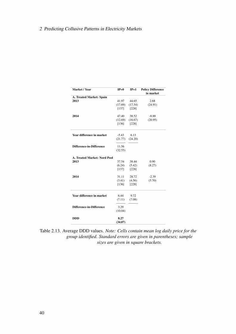
2 Predicting Collusive Patterns in Electricity Markets
Market / Year IP=0 IP=1 Policy Differencein market
A. Treated Market: Spain2013 41.97 44.65 2.68
(17.69) (17.54) (24.91)[137] [228]
2014 47.40 38.52 -8.88(12.69) (16.67) (20.95)[136] [228]
Year difference in market -5.43 6.13(21.77) (24.20)
Difference-in-Difference 11.56(32.55)
A. Treated Market: Nord Pool2013 37.54 38.44 0.90
(6.24) (5.42) (8.27)[137] [228]
2014 31.11 28.72 -2.39(3.41) (4.56) (5.70)[136] [228]
Year difference in market 6.44 9.72(7.11) (7.08)
Difference-in-Difference 3.29(10.04)
DDD 8.27(34.07)
Table 2.13. Average DDD values. Note: Cells contain mean log daily price for thegroup identified. Standard errors are given in parentheses; sample
sizes are given in square brackets.
40

2.6 Results
DDD Estimation DD 2013 DD 2014Variables (1) (2) (3) (4) (5) (6) (7) (8)
IPt ∗Ti ∗ρj0.02120 0.1134** 0.087** 0.1543*** 0.1529*** 0.1404**(0.09) (0.048) (0.04) (0.056) (0.057) (0.055)
Ti-0.00120 0.0871** 0.01930 -0.1629*** -0.1268*** 0.0969*** -0.2044*** 0.24930(0.064) (0.037) (0.024) (0.062) (0.037) (0.035) (0.076) (0.6)
IPt0.010 0.0686*** 0.0154* 0.059*** 0.0466*** 0.0434*** -0.0226 0.02460
(0.024) (0.023) (0.009) (0.021) (0.015) (0.015) (0.012) (0.02)
ρj0.0020 0.2333*** 0.1013*** 0.1887*** 0.1373*** 0.1478***(0.043) (0.053) (0.029) (0.041) (0.036) (0.036)
IPt ∗ρj-0.0080 -0.0523** 0.00780 -0.0792*** -0.0689*** -0.0654***(0.027) (0.022) (0.013) (0.023) (0.019) (0.018)
Ti ∗ρj-0.01890 -0.1173*** -0.0967** -0.0586* -0.072** -0.0666*(0.059) (0.043) (0.039) (0.035) (0.036) (0.036)
Ti ∗ IPt0.01330 -0.0713* -0.03510 -0.0673* -0.05480 -0.05040 0.1047** -0.04420(0.057) (0.039) (0.035) (0.035) (0.036) (0.034) (0.051) (0.032)
AR No Yes Yes Yes Yes Yes Yes YesCONTROL Yes No No Yes Yes Yes Yes Yes
IV Yes No Yes No Yes Yes Yes YesFE Yes No Yes Yes No Yes Yes Yes
Obs 1452 1452 1452 1452 1452 1452 724 728R2 0.069 0.579 0.621 0.648 0.616 0.641 0.648 0.642
Table 2.14. Triple Differences and Difference-in-Differences Results of The Effectof Mandated Auctions on Prices
Column (6) incorporates autoregressive terms, control variables, a quantity esti-mation using instrumental variables and fixed effects. The coefficient of IPt∗Ti∗ρjindicates that the relative price increased by around 15.07 percent in the treated mar-ket during the experimental year. These estimates are highly significant and presentmore robust standard errors compare to a difference-in-differences model (becauseof the double difference).
Columns (7) and (8) show the difference-in-differences results for 2013 and 2014,respectively. As we mentioned previously, two of our identification assumptionswere that the coefficient on the Ti ∗ IPt should be positive for 2013 and not sig-nificant for 2014. Column (7) reveals that the interaction is 11% and is significantat the 5% level. And column (8) reveals that this interaction is statistically non-significant. However, a double differences model only controls for unobservablefactors that affect daily prices and are different between markets, but are constantover time. The triple differences models presented additionally control for unob-servable factors that cause differences in daily prices for both markets to changeover time.
Every column with autoregressive terms shows a similar outcome. The resultsconfirm the conclusion that before the CESUR auctions the Spanish market ex-perienced significant price increases. Specifically, we find a total increase in thedifference of Spanish and Nord Pool markets between 9 and 17% when CESUR
41

2 Predicting Collusive Patterns in Electricity Markets
auctions were introduced. If the objective of mandated auctions is to enhance com-petition, these results seem to contradict the initial assumption and what was statedempirically and theoretically by several authors (Allaz and Vila, 1993; Green, 1999;Wolak, 2000; Woo et al, 2004; Strbac and Wolak, 2017; Wolak, 2017). Becausemandated auctions do not merely affect their own market, it requires careful eval-uation when regulators are considering improving assignative and productive effi-ciencies.
We acknowledge that the model has two important limitations. First, we do nothave data before 2013 for the Nord Pool market, which could enhance our resultsand make them more robust with a large period and a large number of auctions. Sec-ond, microdata about CESUR auctions is incomplete and unavailable, particularlyrelated to the other mechanism in which firms may have affected prices by retiringquantity offers. This could enrich the analysis and explain some of the differencesin CESUR prices.
2.7 Conclusions and Policy Implications
Natural concentration and price volatility are two common characteristics of liber-alized electricity markets. As such, regulation should serve as a tool for deliveringan essential service at an affordable price. In accordance with this line of thinking,several authors have argued that the introduction of fixed-price forward contractobligations increases competition and leads to prices that are closer to marginalcosts. Auctions are usually used as a competitive mechanism to get both efficientsupply and a competitive price. However, even though the auction that assigns thecontracts is competitive enough, bidders who have market power over spot pricesmay influence the final outcome of the auctions by inflating price expectations. Thischapter contributes to the literature on the results of the introduction of mandatedauctions by studying the dynamics of differences in daily prices between two mar-kets: one with regulation and the other without.
Between 2007 and 2013, the Spanish government held the Contratos de Energíapara el Suministro de Último Recurso (CESUR) auctions. The auctions were long-term contracts for a fixed quantity at a price determined by a descendant price auc-tion. This solution emerged as a way to foster liquidity in long-term markets andto stabilize the consumers’ tariff cost. Comparing this market with the Nord Poolmarket (a control group that did not apply this regulation during the same period),we derive the following findings: (i) empirical evidence supports that daily pricessuffered anomalous increases in days surrounding auctions, specifically, during thelast 70 days before each auction. (ii) Using a combination of different methods we
42

2.7 Conclusions and Policy Implications
find that electricity market prices rose by approximately 15 percent in the year whenregulation was introduced in the Spanish market compared to the Nord Pool mar-ket. A number of factors lead us to conclude that the link between this regulationand the price increase is causal. First, the treatment and control groups presentedsimilar trends in the pre-intervention period and second, these two groups presentedsimilar trends once the auction was no longer operational.
Electric companies had several incentives to get higher CESUR prices. Besidesrisk volatility, they received payments and discounts on the energy supplied in thismarket. Clear evidence of ex-post forward premiums is presented in Peña and Ro-driguez (2018), where they find a total premium average of 7.22%. However, themechanisms by which firms could have got higher prices were not closely studied.Firms had two alternatives to influence prices (Fabra and Fabra Utray, 2012): (i) bytaking off their supply offers during the auction (and therefore reducing competitivepressure), and (ii) by affecting parallel market expectations. As a consequence, wefocus on the second mechanism as the first mechanism is hard to analyze due toincomplete and unavailable microdata about the CESUR auctions.
The theoretical model developed herein supports our main conclusions. We de-rive two propositions for the above result: First, the inherent characteristics of mar-kets of this kind serve as an incentive to collusion. In other words, there is a thresh-old at which the set of collusive prices in both markets is a sustainable equilibriumof the perfect subgame. The natural reaction, therefore, is to avoid pro-competitiveregulations. Second, expected exogenous price shocks, which originate once theauction is held, generate a perfect subgame equilibrium where prices are higherthan without it. Conceptually, this suggests that a fixed tariff in a market charac-terized by high volatility – as is the case of the electricity market –induces firms toseek to minimize adverse outcomes by raising their prices.
Our main policy conclusion is that the uncompetitive outcome was originated inthe deficient design of this particular regulatory mechanism. Well-designed mecha-nisms need to take into account the specific characteristics of the electricity market.As argued at the outset to this chapter, the power of Spanish firms to react seemsto stem from anti-competitive structures, a low level of interconnectivity – with justtwo firms concentrating 64% of generation capacity, and a pivotal index rate below110% for more than 5% of the time when the regulation was introduced. Moreover,liberalization exposed the electricity market to high price volatility. A format ofrepeated auctions and fixed prices in an environment of natural concentration andhigh volatility in prices seem to be the main reasons why firms colluded (either toprotect the inherent characteristics of the market or to absorb the volatility risk).Additionally, some particularities of the auction design may have discouraged com-petition. Especially that they knew the ranges of supply excess from where they
43

2 Predicting Collusive Patterns in Electricity Markets
could have intuited their pivotal power. Consequently, regulators who are interestedin limiting market power should mainly be focused on the macro and micro aspectsof this kind of regulation.
We can think of two different alternatives to improve competitive results. Firstand most obvious is that market regulators may consider deregulating the long-termcontract market. However, removing mandated auctions and liberalizing the sectorwhen the market has severe concentration problems and low levels of interconnec-tivity does not seem reasonable. Electricity demand is inelastic per se, therefore,liberalizing where there is no competition may yield to worsening uncompetitiveequilibriums. This is explained by Green (2004), who shows that retail competi-tion when price volatility is high disincentives long-term contracts and produceshigher prices. Furthermore, international empirical evidence is still inconclusiveregarding this point. Mobility between companies tends to be very low and staticdue to contract complexities and high switching costs. Additionally, prices betweenincumbent companies and competitors do not converge in many cases, and pricediscrimination by region is a common practice. Moreover, companies that usuallytake control are incumbents from other industrial sectors or from other regions (seeDefeuilley, 2009 for a detailed analysis on retail competition evidence).
Second, instead of deregulating in order to obtain a competitive situation, whereconsumers can choose between different contract options, an alternative suggestedby some authors is mandatory basic electricity services -wholesale price plus a reg-ulated margin- (see Joskow, 2000). In theory this would provide a competitivebenchmark where consumers could compare options. This mechanism is simple andtransparent, and works as an alternative for the consumer when other options havehigher prices than the market price. However, more research is needed to supportthis statement. Mandatory basic electricity services are based on the assumptionthat electricity markets are competitive enough to be a representative benchmark.But, as we stated in our main results, it would be hard to expect that retailers (whichin the Spanish market are in general holding groups or subsidiaries from companiesthat are present in the generation market) do not seek mechanisms to inflate expecta-tions. An intermediate solution could be the introduction of “Price to Beat” policies(variable prices adapted to the generation cost). In this case, incumbent companiesare only allowed to offer a lower price than the price to beat if, and only if, a certainamount of time has passed or after a share of residential and small business cus-tomers are served by other suppliers (Adib and Zarnikau, 2006 and NERA, 2007).Whatever the alternative, what is clear is that getting completely rid of regulationframeworks leaves market operators with very limited control over concentratedmarkets. Liberalizing where no competition exists is not a prudent decision. Wewant to emphasize that our study does not seek to be critical of the mandated auc-
44
2.7 Conclusions and Policy Implications
tion regulation, quite the opposite: to focus attention on the problem that lies in thedeficient design of this regulatory mechanism and not in the regulation, per se.
Appendix A: Instrumental Variables Tests
As discussed above, a problem that can arise with the OLS estimation is the pres-ence of endogeneity in the quantities of energy (i.e., qt is correlated with µt). Thismeans we cannot infer whether the changes in price and quantity are due to shifts indemand or supply. Wright (1928) suggested that this problem can be addressed byusing curve shifters, i.e. if we find instruments that are related to the demand con-ditions but which do not affect the cost function, then we would be able to identifythe supply correctly.
To do so, we need instruments Z that satisfy two conditions: First, they need tobe correlated with the endogenous variable (cov(Z,q) = 0) and, second, the instru-ments must be orthogonal to the error term (cov(Z,µ) = 0). The second conditioncannot be empirically proven (as we do not know µ); thus, the validity has to be leftto economic reasoning. To test the first condition, we can express the reduced formequation of qt by conducting a two-stage least squares estimation. Therefore, in thefirst stage we can construct an equation such as:
qt = πZ+vi
And using the predicted values qt, we can run a second stage as:
yt = βXt+γIPt+αqt+µt
As qt is uncorrelated with µt, the classic endogeneity assumption remains.Specifically, we propose using a working day dummy variable as our instrument
(which takes a value of 0 on weekends and national holidays, and 1 otherwise).Thus, the assumption we make is that working days are correlated with the quanti-ties demanded but do not directly affect the prices offered.
When we use a vector of instruments z we expect them to satisfy: (1) z is uncor-related with the error term; (2) z is correlated with the instrumental variable; (3) zis strongly correlated with the instrumental variable. The first condition invalidatesthe instrument, the second condition makes the instrument irrelevant, and the thirdcondition makes the model weakly identified.
We use a two-stage least squares estimation to evaluate these conditions. The firstrequirement is difficult to evaluate because we cannot observe the error term. Butwe can test the second requirement using a reduced form with all the exogenous
45

2 Predicting Collusive Patterns in Electricity Markets
variables. As can be seen in Table 2.15, both the quantities for Spain and thosefor Nord Pool satisfy condition (2). Similarly, the F-statistics of the instrumentalvariables (under the null hypothesis that all instrument coefficients are null) validatethe third condition. However, serial correlation, non-stationarity and non-normalityproblems may persist.
First Stage coef std error t P > |t| [0.025 0.975] F-statistic F-valueWorkday Spain 0.1469*** 0.013 11.483 0.00 0.122 0.172 85.49 0.00Workday Nord Pool 0.0636*** 0.011 5.918 0.00 0.042 0.085 18.92 0.00
Table 2.15. Reduced Form q = γz+β1x1 +β2x2. . . +µ
Appendix B: ARMAX Model-Building Process
As we validated the instruments used, the classic endogeneity assumption remains.However, serial correlation, non-stationarity and non-normality problems could per-sist.
The autoregressive moving average (ARMA) is a time-series model that uses twopolynomial terms to describe stationary stochastic processes: autoregressors (AR)and moving averages (MA) (Box et al., 2015). If, in addition, we include exogenousinput terms, we obtain the ARMAX model.
The primary advantage of ARMAX models is that they allow us to correct theeffects of serial correlation (especially present in electricity market prices) whichmay invalidate the estimations. However, models of this kind rely on very strongassumptions that have to be proved before any conclusions can be drawn. Theyinclude:
1. The dependent variable series must be stationary.
2. The residual series must not exhibit serial correlation.
3. The estimated coefficients of exogenous variables must be significantly dif-ferent from zero.
4. The sign of coefficients must be reasonable.
5. Exogenous variables must not exhibit multicollinearity.
Figure 2.7 shows the ARMAX model building approach proposed by Andrewset al. (2013) and based on the practical approach developed originally by Box andJenkins (1970). The extensions applied to ARMAX models involve the introduction
46

2.7 Conclusions and Policy Implications
of new exogenous variables that may disrupt the white-noise pattern of the residualsand which, therefore, might change the order of the autoregressive and movingaverage terms.
Figure 2.7. Armax Building-Model Process
The first assumption of the ARMAX model is that the dependent variable is sta-tionary, i.e., the mean and variance do not change over time. We use an AugmentedDickey-Fuller (ADF) test (Fuller, 1976; Dickey and Fuller 1979) to evaluate thisassumption. Under the null hypothesis, the time-series is a unit root, i.e., it is non-stationary.
Table 2.16 reports the ADF test result. We apply second differences to make thedependent variable time-series stationary. This differencing schema is also appliedto exogenous-variable candidates, which permits correlations to be more stable overtime.
log(PSpain/PNPool) Diff(0) Diff(2)Test Statistic -2.99 -12.29p-value 0.04 0.00Lags Used 14 12Number of Observations Used 381 381Critical Value (1%) -3.45 -3.45Critical Value (5%) -2.87 -2.87Critical Value (10%) -2.57 -2.57
Table 2.16. Augmented Dickey-Fuller Test
We use a forward stepwise regression procedure to identify the most relevant
47

2 Predicting Collusive Patterns in Electricity Markets
exogenous-variable candidates (see Table 2.7). This method seeks to fit a sub-set of attributes by successively incorporating new variables while evaluating theperformance. Those attributes that improve performance can then be maintaineddefinitively.
The ARMAX model works under the assumption that the residuals are whitenoise, i.e., a random sequence that cannot be predicted or, what amounts to thesame thing, that the residuals are stationary and do not exhibit significant serial cor-relation. Serial correlation implies that the error term observations are correlated.Patterns in the error term could bias the significance of the exogenous variables. Asshown in Table 2.17, the ADF test provides evidence that the residuals are station-ary.
ADF Test - ResidualsTest Statistic -11.00p-value 0.00Lags Used 6Number of Observations Used 314Critical Value (1%) -3.45Critical Value (5%) -2.87Critical Value (10%) -2.57
Table 2.17. Residuals Stationarity Test
To test serial correlation, we use the Ljung-Box test (Ljung and Box, 1978) whichchecks under the null hypothesis if the data are independently distributed8. The p-values from the Ljung-Box test (see Table 2.18) support the rejection of the nullhypothesis. This is an indicator that we must add appropriate combinations ofAR/MA terms which are identified from partial autocorrelation and autocorrelationfunctions, respectively.
L1 L2 L3 L4 L5 L6 L7 L8 L9 L10QLJB 77.45 80.33 90.65 94.25 94.33 94.62 97.59 106.64 109.28 109.76p-value 0.00 0.00 0.00 0.00 0.00 0.00 0.00 0.00 0.00 0.00
Table 2.18. Residuals Serial Correlation Test
The autocorrelation function (ACF) describes the correlation between observa-tions and observations at a prior time step. The partial autocorrelation function(PACF) is the autocorrelation between observations in a time series with observa-
8As it tests the overall randomness based on the number of lags, we use the rule proposed byHyndman and Athanasopoulos (2018) where lags are equal to min(10,T/5) for non-seasonal timeseries.
48

2.7 Conclusions and Policy Implications
tions at prior time steps but with the relationships of intervening observations re-moved. If autocorrelation exists, then there is some information that could explainthe movements of the dependent variable but we are not capturing it.
We use the Bayesian Information Criterion (BIC) (Schwarz, 1978) to select theoptimal combination of AR/MA terms. The BIC is based on a likelihood functionwhich also introduces a penalty term to avoid overfitting9.
Based on this criterion, we add seven AR terms and no MA terms. Our model istherefore an ARMAX(7, 0). Figure 2.8 illustrates the ACF and the PACF after theintroduction of the autoregressive terms. This shows that autocorrelation and partialautocorrelation have been removed.
Figure 2.8. Partial Autocorrelation and Autocorrelation Functions
Additionally, in Table 2.19, we present the Ljung-Box test with the new configu-ration which also reveals strong evidence of no serial correlation.
L1 L2 L3 L4 L5 L6 L7 L8 L9 L10QLJB 0.23 0.38 0.55 0.62 0.62 0.81 0.81 0.88 1.82 1.93p-value 0.63 0.83 0.91 0.96 0.99 0.99 0.99 0.99 0.99 0.99
Table 2.19. Residuals Serial Correlation Test with ARMAX(7, 0)
The next assumption in the ARMAX building procedure is that the estimatedcoefficients must be significant. Verification of this is provided by the t-statistics
9BIC = ln(n)k− 2ln(L) where L is the maximized value of the likelihood function of themodel M , n are the number of data points and k the number of variables.
49
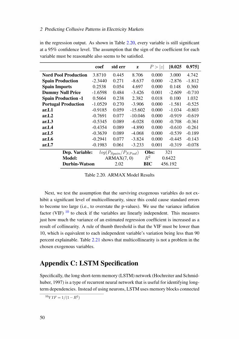
2 Predicting Collusive Patterns in Electricity Markets
in the regression output. As shown in Table 2.20, every variable is still significantat a 95% confidence level. The assumption that the sign of the coefficient for eachvariable must be reasonable also seems to be satisfied.
coef std err z P > |z| [0.025 0.975]
Nord Pool Production 3.8710 0.445 8.706 0.000 3.000 4.742Spain Production -2.3440 0.271 -8.637 0.000 -2.876 -1.812Spain Imports 0.2538 0.054 4.697 0.000 0.148 0.360Dummy Null Price -1.6598 0.484 -3.426 0.001 -2.609 -0.710Spain Production -1 0.5664 0.238 2.382 0.018 0.100 1.032Portugal Production -1.0529 0.270 -3.906 0.000 -1.581 -0.525ar.L1 -0.9185 0.059 -15.602 0.000 -1.034 -0.803ar.L2 -0.7691 0.077 -10.046 0.000 -0.919 -0.619ar.L3 -0.5345 0.089 -6.028 0.000 -0.708 -0.361ar.L4 -0.4354 0.089 -4.890 0.000 -0.610 -0.261ar.L5 -0.3639 0.089 -4.068 0.000 -0.539 -0.189ar.L6 -0.2941 0.077 -3.824 0.000 -0.445 -0.143ar.L7 -0.1983 0.061 -3.233 0.001 -0.319 -0.078
Dep. Variable: log(PSpain/PNPool) Obs: 321Model: ARMAX(7, 0) R2 0.6422Durbin-Watson 2.02 BIC 456.192
Table 2.20. ARMAX Model Results
Next, we test the assumption that the surviving exogenous variables do not ex-hibit a significant level of multicollinearity, since this could cause standard errorsto become too large (i.e., to overstate the p-values). We use the variance inflationfactor (VIF) 10 to check if the variables are linearly independent. This measuresjust how much the variance of an estimated regression coefficient is increased as aresult of collinearity. A rule of thumb threshold is that the VIF must be lower than10, which is equivalent to each independent variable’s variation being less than 90percent explainable. Table 2.21 shows that multicollinearity is not a problem in thechosen exogenous variables.
Appendix C: LSTM Specification
Specifically, the long short-term memory (LSTM) network (Hochreiter and Schmid-huber, 1997) is a type of recurrent neural network that is useful for identifying long-term dependencies. Instead of using neurons, LSTM uses memory blocks connected
10V IF = 1/(1−R2)
50
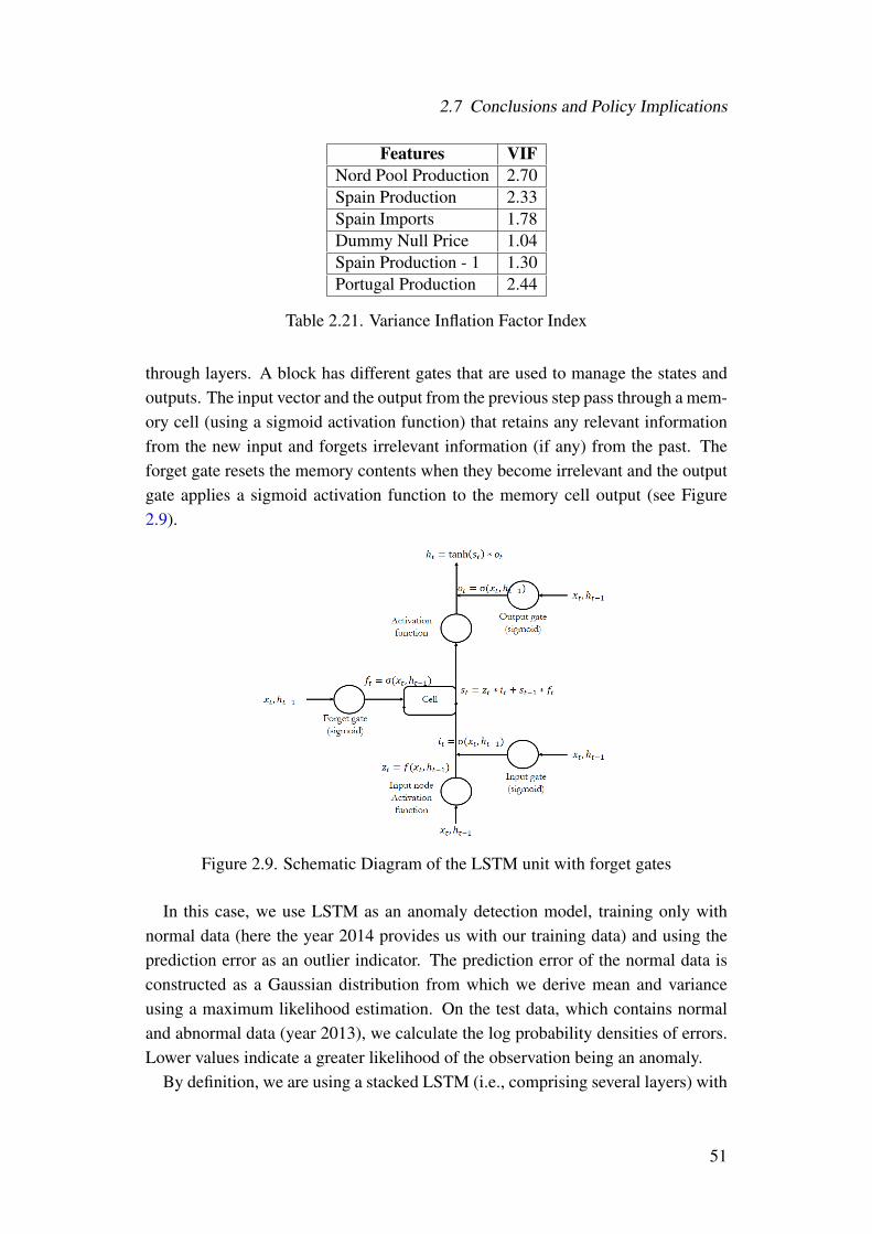
2.7 Conclusions and Policy Implications
Features VIFNord Pool Production 2.70Spain Production 2.33Spain Imports 1.78Dummy Null Price 1.04Spain Production - 1 1.30Portugal Production 2.44
Table 2.21. Variance Inflation Factor Index
through layers. A block has different gates that are used to manage the states andoutputs. The input vector and the output from the previous step pass through a mem-ory cell (using a sigmoid activation function) that retains any relevant informationfrom the new input and forgets irrelevant information (if any) from the past. Theforget gate resets the memory contents when they become irrelevant and the outputgate applies a sigmoid activation function to the memory cell output (see Figure2.9).
Figure 2.9. Schematic Diagram of the LSTM unit with forget gates
In this case, we use LSTM as an anomaly detection model, training only withnormal data (here the year 2014 provides us with our training data) and using theprediction error as an outlier indicator. The prediction error of the normal data isconstructed as a Gaussian distribution from which we derive mean and varianceusing a maximum likelihood estimation. On the test data, which contains normaland abnormal data (year 2013), we calculate the log probability densities of errors.Lower values indicate a greater likelihood of the observation being an anomaly.
By definition, we are using a stacked LSTM (i.e., comprising several layers) with
51

2 Predicting Collusive Patterns in Electricity Markets
memory between batches. This allows us to identify when the state of the networkis reset by using the final state of the sample i of the current batch as the initialstate for i the sample of the next batch. Maintaining the state is crucial in datathat present a long repeated pattern, because if not, the model will be influencedmostly by recent observations. Therefore, we maintain the state over all the trainingbatches, and reset it only when the next batch is about to start, tuning the weightsover different epochs, and allowing the LSTM to store relevant activations in thecell state.
As discussed, for training purposes we use the year 2014, which we assume to bea normal period. In this way, our test data correspond to 2013, for which we haveanomaly data (70 days before each auction) and normal data (remaining observa-tions). Based on this definition, we proceed to employ a typical semi-supervisedoutlier model. Our recurrent neural network comprises three recurrent layers eachmade up of 100 LSTM units, with a final dense output layer with one neuron thatuses a linear activation function. In order to prevent overfitting, we use two differ-ent regularization methods: a dropout of 20% and early stopping set to 2 epochs.The dropout is a regularization method that randomly drops out a number (or per-centage) of layer outputs. It experiments with different architectures of the samenetwork in parallel, which becomes a more robust model as the training process isnoisy and nodes are forced to actually learn a sparse representation (Srivastava etal., 2014). Additionally, we use early stopping which provides a rule of how manyiterations we can run before the learner overfit (i.e., when the test loss starts to beworse than the training loss).
We use an Adagrad optimizer (Duchi et al., 2011) to adapt the learning rate tothe parameters. This is achieved by performing smaller updates for parametersassociated with frequent features, and larger updates for parameters associated withinfrequent features. The main advantage of this optimizer is that it works well withsparse data. As Dean et al. (2012) show, the method greatly improves the robustnessof the stochastic gradient descent optimizer.
We set the loss function as the mean squared error, which is well suited to prob-lems in which real-value quantities are predicted. Thus, we calculate the average ofthe squared differences between the predicted and the real values.
Activation functions define the output of neurons given the previous input. Eachlayer is trained by using the hyperbolic tangent activation function (unless the inputand output gates use sigmoid functions), which has the advantage of being lesslikely to become stuck (as it strongly maps negative inputs to negatives outputs).
In our experiment, we use 50 epochs (i.e., the number of times we go through thetraining set) and a batch size of 50 steps per epoch (i.e., the sample used in eachiteration).
52

2.7 Conclusions and Policy Implications
As we proposed a 70-day time window before auctions as our anomaly pattern,we expect the model to fail to reconstruct the prediction error (fail, that is, in termsof reconstructing a multivariate normal probability density function similar to thatderived from the training error vector). By using a valid-set, we are able to definean optimal threshold that separates anomalies from normal behavior. Finally, thisthreshold is applied to the test error vector where we expect lower values to indicatethat the observation is more likely to be an anomaly.
53


3 Machine Learning Forecasts ofPublic Transport Demand: TheCase Study of Buenos Aires,Argentina
3.1 Introduction
The use of smart cards is becoming increasingly popular on public transport ser-vices. They are especially convenient for users as they reduce their transactionalcosts and boarding times, whereas for bus companies, they enable them to plantheir schedules more effectively, improve commercial bus speeds, while indirectlyallow them to reduce personnel and maintenance costs. But the cards have a furtheradvantage that has yet to be exploited: they provide massive amounts of informa-tion ranging from tariffs to GPS-generated mobility patterns. Such a rich seam ofdata, if mined properly, should have great policy implications for public transporta-tion authorities, sector regulators, transport operators and other interested parties,as well as the public in general.
Many recent studies stress the potential of smart card data as a tool for transportmanagement and planning (Blythe, 2004; Bagchi and White, 2005; Agard et al.,2006; Utsunomiya et al., 2006; Morency et al., 2007; Pelletier et al., 2011; Mu-nizaga and Palma, 2012; Ma et al., 2013; Kusakabe and Asakura, 2014; Briand etal., 2017; Ma et al., 2017, Li et al., 2018). Here, a particularly interesting dimensionof analysis is estimating demand given that smart cards record the commuting char-acteristics of each passenger, including data about travel dates, time of day, originand destination, journey times, etc. Indeed, if transport authorities and regulatorscould exploit this demand information, they would be able to optimize the transportnetwork as a whole. Several examples can be found: Dou et al. (2015) use smartcard data from the public transport service in Queensland city to predict individ-ual mobility patterns. Zhou et al. (2017a) analyze the responses of passengers toweather conditions by combining meteorological data with large-scale smart card
55

3 Machine Learning Forecasts of Public Transport Demand
data in the city of Shenzhen. Zhou et al. (2017b) use information of card swip-ing times to estimate bus arrival more precisely in Beijing. Kumar et al. (2018)use several features collected from the smart card data in the Minneapolis transportintegrated network to develop an innovative method for trip chaining. Huang etal. (2018) combine mobile phone data, subway smart card data and taxi GPS datafrom Shenzhen to predict real time urban travel demand. Zhao et al. (2018) utilizetransit smart card records from the rail-based system in London to predict the nexttrip within a day and its attributes. Ingvardson et al. (2018) analyze passenger ar-rivals and waiting times at rail stations in Copenhagen using smart card data fromthe public transport system in Denmark. Zhang et al. (2018) fusion self-reportedrevealed preferences data with smart card data collected from the Guangzhou citymetro system to forecast metro passengers’ path choices.
To date, however, few studies have resorted to the use of smart cards for theirinput data to predict demand and elasticities. Those that have include Seaborn et al.(2009), Munizaga and Palma (2012), Tao et al. (2014), Tao et al. (2016). One ofthe most innovative examples is provided by Arana et al. (2014) who analyze smartcard data to predict demand. They use multiple linear regression analysis to assessthe impact of weather conditions on the number of trips taken and the underlyingmotives for these trips. However, it was hard to find literature related to fare impacton public transport demand using smart card data. Examples are de Grange et al.(2013) who estimate demand elasticities for the integrated system in Santiago deChile and Wang et al. (2015) who analyze fare changes in the Beijing Metro tocalculate price demand elasticity. Nevertheless, demand elasticity is a problem thateconomic literature has widely aboard using other sources (Just to mention someexamples: Goodwin, 1992; Preston, 1998; Nijkamp and Pepping, 1998, Hensher,1998; FitzRoy and Smith, 1998; Bonnel and Chausse, 2000; Hanly et al., 2002;Matas, 2004; Bresson et al., 2003, 2004; Balcombe et al., 2004; Paulley et al.,2006; García-Ferrer et al., 2006; Holmgren, 2007; Crotte, 2008; Graham et al.,2009; Albalate and Bel, 2010; Tsai et al., 2014, Tsai and Mulley, 2014).
Regarding time-series forecasts of public transport, quite number of authors ap-ply Autoregressive Moving Average regressions (ARMA). This kind of model andits variations maintain the interpretation of traditional linear models but also takeinto account the residuals pattern. Examples are Ahmed and Cook (1979) who ap-ply ARMA models to forecast traffic state in USA, Williams et al. (1998) who useSARIMA models in traffic seasonal flows, Suwardo et al. (2010) apply ARIMAmodels to predict bus travel time in Malaysia, Gong et al. (2014) who use aSARIMA model to predict the arrival passengers and the number of waiting passen-gers, Xue et al. (2015) who forecast short-term passenger demand based on smartcard data from Shenzhen, China and Milenkovic et al. (2018) who use SARIMA
56

3.1 Introduction
models to forecast railway passenger flows in Serbia. However, most analyses inthe literature employ linear models, which means they make demand predictionsusing techniques that are better suited for finding causal relationships. Kremers etal. (2002) show that from 79 studies related to public transport demand, 55 modelswere estimated using log-linear models and 24 used linear models.
In this study, our focus is very clearly on methods that enhance prediction capa-bilities as opposed to the assessment of marginal effects on target variables. More-over, traditional models fail to take into account the importance of performance interms of out-of-sample errors (Mullainathan and Spiess, 2017). Their focus on in-sample data is not an optimal approach to forecasting demand. Here, in contrast,we highlight the importance of testing a prediction model with out-of-sample datafrom smart cards, given that the results of a forecast and the fulfillment of actualevents may differ.
The objectives of this chapter can therefore be clearly stated. First, we presentvarious supervised machine learning (SML) techniques for predicting public trans-port demand using smart card data. SML techniques train models using historicaldata in such a way that they learn from the patterns that emerge. However, moreimportantly, machine learning techniques are validated with test data so that theirreal predictive power can be determined. Second, we then compare these results tolinear models outcomes to determine the gain in performance achieved with SMLtechniques. The comparative analysis is focused in three aspects: interpretability,predictive power and demand elasticity.
It follows, therefore, that machine learning (ML) algorithms are specifically de-signed for making predictions, while linear models are not (Xie et al., 2003; Zhangand Xie, 2008; Kleinberg et al., 2015; Zhao et al., 2018). Moreover, ML are ableto exploit several data types and complexities. But perhaps their main advantage isthe fact that computers can be programmed to learn from data, revealing previouslyhidden findings as they discover historical relationships and trends. ML techniquescan improve the accuracy of predictions by removing noise and by taking into ac-count many types of estimation, although not necessarily without bias. Moreover,ML allows for a wide range of data, even when we have more predictors than ob-servations, and it admits almost every type of functional form when using decisiontrees, ensuring a large interaction depth between variables. Of course, the down-side of ML techniques is biased coefficients; however, if our main concern is theaccuracy of the prediction, then any concerns regarding biased estimators becomeirrelevant.
Thus, number of recent studies have suggested that machine learning algorithmsare well suited to predict travel behavior (Omrani et al., 2013; Omrani, 2015; Ha-genauer and Helbich, 2017; Golshani et al., 2018; Wang and Ross, 2018; Zhao
57

3 Machine Learning Forecasts of Public Transport Demand
et al., 2018; Gu et al., 2018). There are several applications of machine learningtechniques related to predicting traffic flow, traffic speed, travel time and travel be-havior. For instance, Yu et al. (2011) compared several supervised models to predictbus arrival times and bus stops using survey data from Hong Kong. Pitombo et al.(2017) find that tree based decision models outperform traditional gravity modelsin predicting destination choices. Ke et al. (2017) analyze on-demand ride ser-vice data in Hangzhou city and try to forecast short-term passenger demand via along short-term memory network. Liu and Chen (2017) also use supervised deeplearning models but to predict the hourly passenger flow in Xiamen city. Similarly,Wu et al. (2018) utilize deep learning models to explore traffic flow predictionby exploiting detectors data from an interstate highway. Xu et al. (2018) forecastbike sharing travel demand using a deep-learning approach and data collected formNanjing city. Sekula et al. (2018) compare diverse supervised models and predicthourly traffic volumes by combining data from automatic traffic recording and sev-eral data sources from Maryland city. Wang et al. (2019) predict traffic speed witha variety of supervised models, exploiting data collected from automatic vehicleidentification detectors in Xuancheng city. Ma et al. (2019) use a combination ofunsupervised and supervised algorithms to predict bus travel time by using vehicletrajectories and bus smart card data. Liu et al. (2019) compare several deep learningarchitectures to predict short-term metro passenger flow using data collected fromthe Nanjing city metro system. Other applications of machine learning techniquesare related to driving safety and efficiency: Yuang and Cheu (2003) use severalSVM classifiers to detect arterial and freeway incidents in peak periods in surveydata from Singapore. Guo et al. (2018) fusion multiple supervised models to predictshort-term traffic and capture traffic uncertainties such as incidents and accidents.Bejani and Ghatee (2018) propose a driving style evaluation system by comparinga variety of supervised algorithms based on smartphone sensor data. Similarly, Yiet al. (2019) use smartphone data to develop a personalized driving state recogni-tion system using several supervised classifiers. In this way, given that the literatureinforms us that SML methods are better than traditional econometric predictiontechniques, our hypothesis is that this should also be illustrated in transport demandpredictions based on data retrieved from smart cards.
Here, we study the case of the Autonomous City of Buenos Aires (CABA inits Spanish acronym), the capital city of Argentina. We analyze the use of theSUBE (Sistema Único de Boleto Electrónico), a smart card employed on the city’spublic transport services (train, metro and bus) since 2009, and which has now beenextended for use throughout the country. The card (similar in many respects to acredit card) collects multiple details about travelers and the journeys they make, andprovides information about the location of vehicles using GPS and is, therefore, an
58
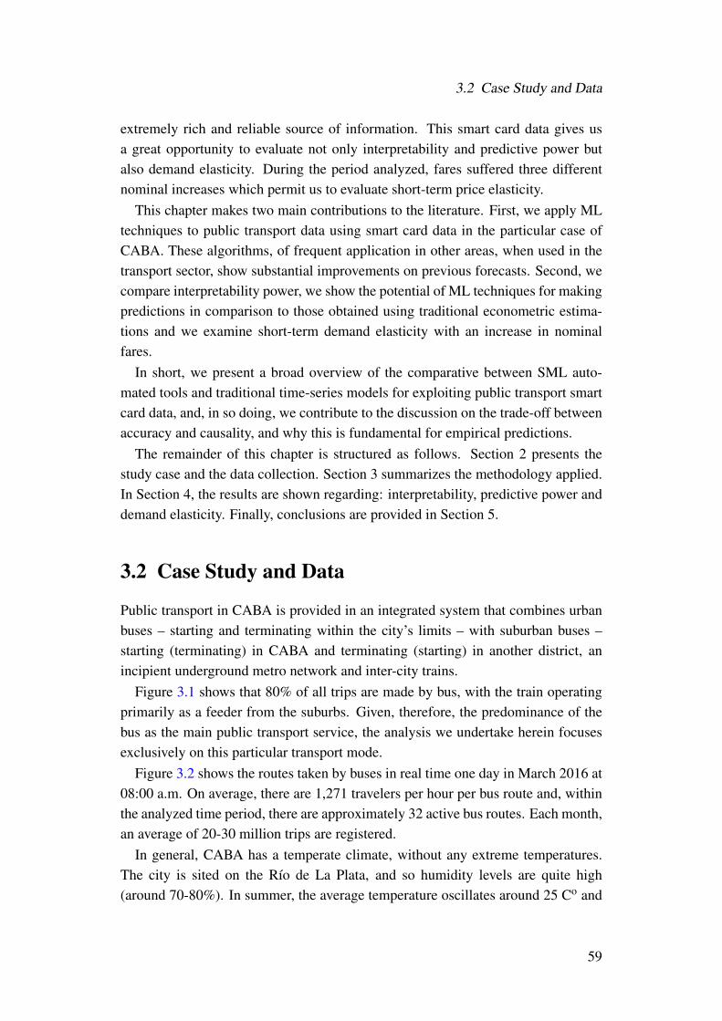
3.2 Case Study and Data
extremely rich and reliable source of information. This smart card data gives usa great opportunity to evaluate not only interpretability and predictive power butalso demand elasticity. During the period analyzed, fares suffered three differentnominal increases which permit us to evaluate short-term price elasticity.
This chapter makes two main contributions to the literature. First, we apply MLtechniques to public transport data using smart card data in the particular case ofCABA. These algorithms, of frequent application in other areas, when used in thetransport sector, show substantial improvements on previous forecasts. Second, wecompare interpretability power, we show the potential of ML techniques for makingpredictions in comparison to those obtained using traditional econometric estima-tions and we examine short-term demand elasticity with an increase in nominalfares.
In short, we present a broad overview of the comparative between SML auto-mated tools and traditional time-series models for exploiting public transport smartcard data, and, in so doing, we contribute to the discussion on the trade-off betweenaccuracy and causality, and why this is fundamental for empirical predictions.
The remainder of this chapter is structured as follows. Section 2 presents thestudy case and the data collection. Section 3 summarizes the methodology applied.In Section 4, the results are shown regarding: interpretability, predictive power anddemand elasticity. Finally, conclusions are provided in Section 5.
3.2 Case Study and Data
Public transport in CABA is provided in an integrated system that combines urbanbuses – starting and terminating within the city’s limits – with suburban buses –starting (terminating) in CABA and terminating (starting) in another district, anincipient underground metro network and inter-city trains.
Figure 3.1 shows that 80% of all trips are made by bus, with the train operatingprimarily as a feeder from the suburbs. Given, therefore, the predominance of thebus as the main public transport service, the analysis we undertake herein focusesexclusively on this particular transport mode.
Figure 3.2 shows the routes taken by buses in real time one day in March 2016 at08:00 a.m. On average, there are 1,271 travelers per hour per bus route and, withinthe analyzed time period, there are approximately 32 active bus routes. Each month,an average of 20-30 million trips are registered.
In general, CABA has a temperate climate, without any extreme temperatures.The city is sited on the Río de La Plata, and so humidity levels are quite high(around 70-80%). In summer, the average temperature oscillates around 25 Co and
59

3 Machine Learning Forecasts of Public Transport Demand
Figure 3.1. Domiciliary Mobility Survey (2013)
Figure 3.2. Location of CABA
60
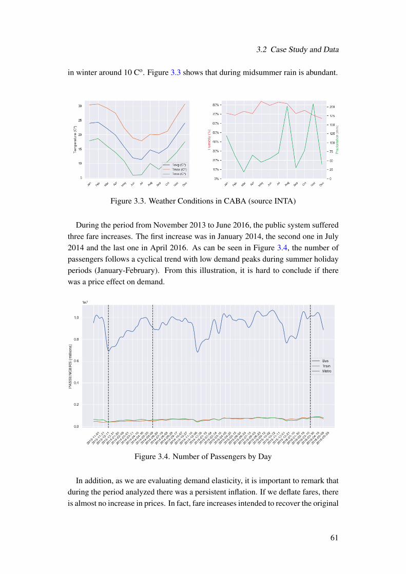
3.2 Case Study and Data
in winter around 10 Co. Figure 3.3 shows that during midsummer rain is abundant.
Figure 3.3. Weather Conditions in CABA (source INTA)
During the period from November 2013 to June 2016, the public system sufferedthree fare increases. The first increase was in January 2014, the second one in July2014 and the last one in April 2016. As can be seen in Figure 3.4, the number ofpassengers follows a cyclical trend with low demand peaks during summer holidayperiods (January-February). From this illustration, it is hard to conclude if therewas a price effect on demand.
Figure 3.4. Number of Passengers by Day
In addition, as we are evaluating demand elasticity, it is important to remark thatduring the period analyzed there was a persistent inflation. If we deflate fares, thereis almost no increase in prices. In fact, fare increases intended to recover the original
61

3 Machine Learning Forecasts of Public Transport Demand
real value. For instance, the weighted average nominal increase in May 2016 wasaround 80%. However, the real increase was only 1-dollar cent. See Figure 3.5.
Figure 3.5. Nominal and Real Fares Evolution
This money illusion effect give us a great opportunity to evaluate the nominaldemand elasticity. As the real effect was negligible, we would expect that demandhave not decreased with higher nominal fares. Any other result should be consideredpart of a money illusion effect. The last part of this study is therefore going to bededicated to analyze the demand behavior.
3.2.1 SUBE
We use data from the SUBE, sorted primarily by bus route and by hour during theperiod that extends from September 2013 to June 2016. It should be borne in mindthat the bus system has undergone no modifications or developments since 2012, inaccordance with Ministerial Resolution 422/12. This means that during the periodanalyzed, the system’s supply did not vary in terms of routes, vehicles, frequencyof services or quality (all buses being identical as they have to respect the techni-cal specifications stipulated under provincial law). In addition, use of the SUBE isobligatory for all companies and it is not possible to use an alternative form of pay-ment. These facts are significant with regards to potential problems of endogeneity,given that we seek to predict demand. Furthermore, note that competition betweenfirms operating the system is meaningless because the government controls not onlytheir costs but their profits too (as well as defining service quality and quantity andfares).
62

3.3 Methodology
3.2.2 Weather
All data concerning weather conditions are provided by the nearest climate stations,under the management of INTA (National Institute of Agricultural Technology).There are three monitoring stations in the study area that report climate data everyfifteen minutes. Several spectra of variables are available, but we use those of tem-perature, wind and precipitation so that we can compare our outcomes with thoseof Arana et al. (2014).
3.2.3 Economics
We use monthly wage index historical series (base 2012=100) and the economic ac-tivity monthly estimator from Instituto Nacional de Estadísticas y Censos (INDEC).As the price index during some periods is not fully reliable, we use the consumerprice index from the statistic institute of Buenos Aires city. From the same sourcewe also obtained the automotive fleet evolution of the city. From Confederaciónde Entidades del Comercio de Hidrocarburos y Afines de la República Argentina(CECHA), we got the daily petrol final price. Finally, we use an online source toget exchange rate series1.
3.3 Methodology
3.3.1 Basic Statistics
First of all, we evaluate if passenger data is stationary, i.e. if the statistical propertiesdo not change over time (mean, variance, etc.). In other words, we would expectseries without trends, with constant variance and no seasonality or autocorrelation(weak stationarity process definition). Several statistical forecasting methods arebased on this assumption (e.g., ARIMA models). Without this property, modelscould provide meaningless sample statistics and invalid estimations.
In Figure 3.6 we decompose2 the passenger series to evaluate how it behaves.It does not seem to exhibit a long-run trend effect and decomposed residuals alsoseem quite random. However, the series exhibits a strong cyclical pattern. Thisseasonality is apparently due to the weekdays-weekends effect. Every weekend,there is a massive fall in passengers, as you can appreciate in Figure 3.7, where wezoom the first weeks of the series.
1source:investing.com2we apply a multiplicative decomposition expressed as: y = x∗ trend∗seasonality ∗error
63

3 Machine Learning Forecasts of Public Transport Demand
Figure 3.6. Multiplicative Decomposition
Figure 3.7. Seasonality Pattern
One popular stationarity test is the Augmented Dickey-Fuller test –ADF- (Fuller,1976; Dickey and Fuller, 1979). Under the null hypothesis the time-series is aunit root, i.e. not only the shocks have permanent effects but also the variance istime dependent. If the null hypothesis is not rejected, we should apply differenceoperators to the series.
Despite the ADF rejected the null hypothesis (i.e., the series does not follow a unitroot process), we take the seven difference of the series to smooth the seasonalityeffect.
As can be appreciated in Figure 3.8, the passenger series looks more stable and itseems to follow a stationarity process. There are still some strong peaks which areactually related to general strikes (specifically, 10th April 2014, 31st March 2015,9th June 2015). The results of the ADF test are reported in Table 3.1.
We also check stationarity on the predictors to avoid spurious regressions, andwe differentiate if it is needed (Newbold and Granger, 1974).
Additionally, we run a Darwin-Watson Test –DW- (Durbin and Watson; 1950,1951, 1971) to check autocorrelation. The test statistic is approximately equal to2 ∗ (1− r) where r is the sample autocorrelation of the residuals. Thus, for r = 0,indicating no serial correlation, the test statistic equals 2. We get a DW of 1.872,therefore, we do not find evidence of serial correlation.
64

3.3 Methodology
Figure 3.8. Series Stationarity
Passengerst−Passengerst−7Test Statistic -14.45p-value 0.00Lags Used 7Number of Observations Used 928Critical Value (1%) -3.44Critical Value (5%) -2.86Critical Value (10%) -2.57
Table 3.1. Augmented Dickey-Fuller Test
65

3 Machine Learning Forecasts of Public Transport Demand
3.3.2 Ordinary Least Squares
Our first model is a log linear Ordinary Least Squares (OLS). The initial model canbe stated as:
log(yt) = βxt+ ε
Where yt is the seven difference of number of passengers in the period t, and xis the vector that represents explanatory variables.
To complete the comparative analysis, we take as our starting point the predictivestudy reported by Arana et al. (2014), which undertake a multiple linear regressionanalysis, using smart card and weather data, to predict demand. We also introducea number of additional considerations which enriches our estimations considerably.The results of the OLS regression are shown in Table 3.2.
coef std err t P > |t| [0.025 0.975]
National Day -0.9238 0.114 -8.070 0.000 -1.149 -0.699Workday -0.0930 0.056 -1.666 0.096 -0.203 0.017Strike -3.0036 0.345 -8.706 0.000 -3.681 -2.326Government -0.0000 0.000 -1.454 0.146 -0.000 0.000Precipitation (mm) -0.0045 0.002 -2.544 0.011 -0.008 -0.001Temperature (Co) 0.0129 0.009 1.516 0.130 -0.004 0.030Strong Wind 0.2765 0.252 1.098 0.273 -0.218 0.771Exchange Rate (ARS/USD) 0.0457 0.557 0.082 0.935 -1.048 1.140Economic Activity Index -0.0138 0.016 -0.881 0.378 -0.045 0.017Real Wage Index -9.4126 6.108 -1.541 0.124 -21.405 2.580Relative Fare (Metro/Bus) 2.5289 0.907 2.787 0.005 0.747 4.311Oil Final Price (ARS) -0.9386 0.534 -1.758 0.079 -1.987 0.110Relative Fare (Train/Bus) 0.2102 0.093 2.248 0.025 0.027 0.394Fleet 0.0004 0.000 6.376 0.000 0.000 0.000Nominal Fare (ARS) -0.1180 0.101 -1.172 0.241 -0.316 0.080Trend 0.0001 0.000 0.914 0.361 -0.000 0.000Vehicle Fleet 0.0000 0.000 0.961 0.337 -0.000 0.000
Dep. Variable: Pax - Pax(-7) Model: OLSNo. Observations: 701 R-squared: 0.301Durbin-Watson: 1.872 Adj. R-squared: 0.285
Table 3.2. OLS Regression Results
We proceeded to include several time variables (Hauer, 1971), which we deemimportant for quantifying demand and which are essential to ensure a good qualityanalysis. We added a dummy variable controlling a government transition (Gov-ernment) and a dummy variable related to general strikes (Strike). We incorporated
66

3.3 Methodology
a variable that differentiates working days from non-working days -i.e., Saturdays,Sundays- (Workday) and a variable for national holidays (National Day).
We then added the three weather variables considered by Arana et al. (2014)with slight differences. We included as a dummy the notion of Strong Wind, that is,a wind with a velocity greater than 50 km/hour on the Beaufort scale, as we con-sider it to be more readily interpretable in terms of its explanatory power. Also weintroduce the precipitation level (Precipitation (mm)) and the average temperature(Temperature (Co)).
We complemented the above with the only offer relevant variable, namely Fleet,which computes the total number of buses circulating each day. All the other char-acteristics (e.g., quality, new routes, etc.) are static and, therefore, we assume thereis no endogeneity between supply and demand.
The last variables we introduced are related to the bus fare, prices and the eco-nomic situation. Following Holmgren (2007) we added a real wage index to takeinto account the income-elasticity (Real Wage Index), the price of petrol (Oil Fi-nal Price (ARS)) and the relative price between bus and substitutes (Relative Fare(Metro/Bus) and Relative Fare (Train/Bus)). Finally, we included a variable re-lated to the economic activity in CABA (Economic Activity Index), the nominal fare(Nominal Fare (ARS)) and a trend variable.
All the variables present their expected signs, however not all of them are signif-icant. In summary, during national days and strikes, less passengers are recorded.Precipitation is the only weather variable which seems to have a significant impact.The results also show that bus is a substitute service for train and metro. Addition-ally, the size of the fleet presents a positive relation with a larger number of travelersand there is no evidence of income-elasticity effects. Finally, the nominal fare doesnot show any significant impact.
The results of this OLS time-series model could however be very influenced byserial correlation, i.e. the error term observations could be correlated. A pattern inthe error term (when we are assuming that it is white noise) could bias the signifi-cance of the explanatory variables.
As many time-series models work under the assumption that residuals are whitenoise (i.e., a random sequence which cannot be predicted), we should evaluate ifthey are stationary and if they do not present any serial correlation problem. Fortesting stationarity, we apply the ADF test which rejects the null hypothesis of unitroot (see Table 3.3).
Now we know that the errors are stationary, we evaluate serial correlation. Weapply the Ljung-Box test (Ljung and Box, 1978) which checks if whether any ofa group of autocorrelations of the series are statistically different from zero (underthe null hypothesis the data is independently distributed). It tests the overall ran-
67

3 Machine Learning Forecasts of Public Transport Demand
ResidualsTest Statistic -11.39p-value 0.00Lags Used 7Number of Observations Used 693Critical Value (1%) -3.44Critical Value (5%) -2.86Critical Value (10%) -2.57
Table 3.3. OLS: Augmented Dickey-Fuller Test
domness based on a number of lags. We use the rule proposed by Hyndman andAthanasopoulos (2018) and set the number of lags equal to min(2m,T/5), wherem is the period of seasonality and T is the length of the time series.
L1 L2 L3 L4 L5 L6 L7 L8 L9 L10 L11 L12 L13 L14QLJB 3.78 4.32 4.67 4.80 4.85 12.50 73.68 74.51 74.79 75.65 75.88 76.17 76.55 76.89pvalue 0.05 0.12 0.20 0.31 0.43 0.05 0.00 0.00 0.00 0.00 0.00 0.00 0.00 0.00
Table 3.4. OLS: Serial Correlation
As shown in Table 3.4, we reject the null hypothesis of no serial correlation forseveral lags and we cannot consequently affirm that residuals are white noise. Be-fore continuing with the machine learning algorithms, we are therefore going tointroduce a SARIMAX model.
3.3.3 SARIMAX
Autoregressive Integrated Moving Average (ARIMA) is a time-series model whichuses two polynomials terms to describe stationary stochastic processes: autoregres-sors (AR) and moving averages (MA), and an initial differentiating step. SeasonalAutoregressive Integrated Moving Average (SARIMA) is an extension of ARIMAmodels which explicitly takes into account seasonal components: ARIMA(p,d,q)
x(P,D,Q)s where P is the number of seasonal autoregressive (SAR) terms, D isthe number of seasonal differences, and Q the number of seasonal moving average(SMA). If we also add exogenous input terms we get the SARIMAX definition.
For choosing the correct model specification we have to evaluate the autocorre-lation function (ACF) and the partial autocorrelation function (PACF). The ACFdescribes the autocorrelation between observations and observations at a prior timestep. The PACF is the autocorrelation between observations in a time series withobservations at prior time steps with the relationships of intervening observationsremoved. When autocorrelation is present, the error term follows a pattern, invali-
68

3.3 Methodology
dating essential assumptions of time-series models. If autocorrelation exists, thereis some information that could be explaining the movements of the dependent vari-able and we are not able to capture. In Figure 3.9 we plot the ACF and the PACF.
Figure 3.9. Series Stationarity
The passenger variable does not seem to show a strong autocorrelation with daysbefore. Remember that now the dependent variable is the difference between thenumber of passengers and the number of passengers one week before. With this inmind, there is some correlation with the same difference but one week before. Wetherefore add an autoregressive variable of order 7 (AR7) to the predictors. Besides,in the partial autocorrelation plot, we can appreciate a seasonality pattern every 7lags. This can be solved by using seasonality ARIMA models, particularly, byapplying moving averages terms for the cyclical pattern (SMA).
Statistic p-value
Ljung-Box (Q) 24.28 0.98
Table 3.5. SARIMAX: Serial Correlation
Table 3.5 reports the Ljung-Box test after we added to the model the temporalterms. As can be appreciated, we cannot now reject the null hypothesis of no serial
69

3 Machine Learning Forecasts of Public Transport Demand
correlation. Knowing that the residuals are white noise, we therefore present theresults of the SARIMAX model (see Table 3.6)3.
coef std err z P > |z| [0.025 0.975]
National Day -0.9210 0.123 -7.506 0.000 -1.162 -0.681Strike -3.3073 0.075 -43.891 0.000 -3.455 -3.160Precipitation (mm) -0.0048 0.002 -2.155 0.031 -0.009 -0.000Relative Fare (Metro/Bus) 1.9968 0.877 2.278 0.023 0.279 3.715Relative Fare (Train/Bus) 0.1625 0.059 2.774 0.006 0.048 0.277Fleet 0.0003 0.000 8.084 0.000 0.000 0.000Nominal Fare (ARS) -0.0865 0.044 -1.984 0.047 -0.172 -0.001AR7 -0.4725 0.015 -32.131 0.000 -0.501 -0.444ma.S.L7 0.0789 0.020 3.889 0.000 0.039 0.119ma.S.L14 -0.2104 0.025 -8.277 0.000 -0.260 -0.161
Dep. Variable: Pax - Pax(-7) Model: SARIMAX(1, 0, 2, 7)No. Observations: 701 R-squared: 0.532Ljung-Box (Q): 24.28 Prob(Q): 0.98
Table 3.6. SARIMAX Model Results
In comparison with the OLS model, we obtain quite similar results. But now,either AR7 and the seasonal MA are very significant.
However, this tells us nothing in terms of demand forecasts; indeed, causalitywould appear not to be directly relevant. Clearly, we would all expect the numberof passengers to decrease on national days and for rain to act as a deterrent to mo-bility. What bus operators and transport regulators need also to know is the likelynumber of passengers at any specific time, that is, they need accurate forecasts. Inother words, they need answers to such questions as: How many passengers willthere be if it rains tomorrow? The smart card is an excellent tool – a highly innova-tive technology – that provides us with daily feedback for use in predictive analyses.Smart cards facilitate the construction of an unparalleled base learner that is con-stantly improving itself. Given the availability of these data, the next step is to startusing algorithms that can exploit this advantage.
Therefore, we are going to compare traditional models in three ways: inter-pretability, predictive power in out-of-sample data, and demand-elasticity estima-tion. But before, let us briefly introduce some of the most popular supervised ma-chine learning algorithms.
3It is important to remark that we followes the practical approach proposed by Andrews et al.(2013) to select the appropriate SARIMAX model.
70

3.3 Methodology
3.3.4 Machine Learning Algorithms
Penalized Linear Regressions
Penalized linear regression (PLR) is a method designed to overcome some of theproblems associated with OLS, basically that of overfitting (i.e., the impossibilityto generalize well from the training data to out-of-sample data). They allow degreesof freedom to be reduced to fit data and model complexity. They are especially goodmethods when degrees of freedom are tight.
We adopt a shrinkage approach in our estimations, that is, we augment the errorcriteria that is being minimized with a data-independent penalty term (or regulariza-tion parameter α). The problem we seek to solve by using α is a problem inherentto all predictions, namely, the trade-off between bias and variance (or overfitting).P (β) is the penalty function that can take several forms. The most common are theridge regression (Tikhonov and Arsenin, 1977)-which uses the squares of β- andthe lasso regression (Santosa and Symes, 1986)-which uses the absolute values ofβ. Elastic net regression combines these two methods, as shown below:
β∗0 ,β∗ = argminβ∗0 ,β∗(
1
m
m
∑i=1
(yi− (β0 +xiβ))2 +λαL|β|+(1−λ)αRβTβ)
So that when λ = 1, it corresponds to a lasso penalization, and when λ = 0, itcorresponds to a ridge regression.
In summary, here, what we seek is a good quality trade-off between bias andvariance. If we can achieve a greater reduction in variance than the correspondingincrease in bias, then we can obtain higher accuracy. To choose α we applied theElastic net regression with iterative fitting along a regularization path (using 5-Foldscross validation). The α that minimizes the mean-squared error is 0.21, as can beseen in the Figure 3.10.
Binary Decision Trees
A decision tree consists of a set of tree-structured decisions that takes Boolean de-cisions. A set of features is tested from the root node, and by a recursive process(which optimizes the splits) we obtain the prediction when the leaf node is reached.The disadvantages of this kind of model are that it tends to be noisy and to overfit(Last et al., 2002; Quinlan, 2014). To avoid these problems, we present a varietyof ensemble methods. Ensemble methods use a set of algorithms that combine dif-ferent predictions (base learners like binary decision trees) and the combination ofthese results offers better outcomes than those obtained from random guessing.
71

3 Machine Learning Forecasts of Public Transport Demand
Figure 3.10. Elastic Net 5-Fold CV
Aggregation Algorithm (Bagging)
Bagging (Breiman, 1996) uses bootstrap samples (i.e., samples with repetition)from the training data and then it trains a base-learner in each of these samples.The combination of independent base learners leads to a decrease in the loss func-tion. Finally, it takes a simple average of their outcomes.
Bagging primarily addresses the variance error, but it has some issues with thebias error. This means that it needs good depth (given that it is a simple model thatgenerates splitting points concentrated in the same place).
Random Forest
Bagging only constructs trees using bootstrap samples of data, whereas random for-est –RF-(Breiman, 2001) also uses a random sample on predictors before each nodeis split, until the tree conditions are fulfilled. This ensures greater independencebetween trees, because of the combination of bootstrap samples and random drawsof predictors. Consequently, we can take advantage of averaging a large number oftrees (and so obtain better levels of variance reduction). Similarly, we can gain interms of bias reduction, because we can employ a very large number of predictors(more even than the number of observations), and local feature predictors can playa role in tree construction.
In conclusion, this method has all the advantages of bagging combined with alower propensity to overfit (each tree fits, or overfits, a part of the training set, and inthe end these errors cancel each other out, at least partially), and, as we see below, itis easier to tune than gradient boosting (GB). Thus, RF works particularly well with
72

3.4 Results
fully grown decision trees (low bias, high variance). Moreover, it tackles the errorreduction task in the opposite way, that is, by reducing variance. In contrast to GB,trees are made uncorrelated to maximize the decrease in variance, but RF cannotreduce bias (which is slightly higher than that of a simple binary tree). Hence, theneed for large unpruned trees, so that the bias is as low as possible at the outset.
In contrast to decision trees, we can reduce the number of observations in theterminal nodes, because RF is less likely to overfit. However, we maintain the samesplits rule. Finally, we have to set the number of predictors sampled, and this is akey tuning parameter that will affect performance. There exist several rules, but themost common is k = log2(n) + 1 (as recommended by Breiman, 2001).
Gradient Boosting
What GB (Friedman, 2001) does is to train a set of trees, where every tree is trainedon the error of the previous ensemble models. GB starts in the same way as bag-ging, but it focuses on the areas that present most mistakes. This gives a betterapproximation, without the need for greater depth, which is an essential advantage.In contrast with RF, GB works well when based on weak learners in terms of highbias and low variance (even as small as decision stumps). GB reduces the error pri-marily by reducing bias, and to some extent the variance, by aggregating the outputfrom many models.
In summary, RF trains with a random sample of data in addition to randomizingfeatures. It relies on this randomization to give a better generalization performanceon out-of-sample data. GB, on the other hand, additionally seeks to find the optimallinear combination of trees, where the final model is the weighted sum of predictionsof individual trees applied to the training data.
3.4 Results
We evaluate the results in three different ways: interpretability, predictive powerand demand elasticity. In doing so, we split our data-set in three sequential samples(see Figure 3.11):
1. Test (54 obs): This is the period with the last fare increase (approximately80%) and which we are going to use at the end of the study to test our hy-pothesis about demand elasticity (from April 2016 to June 2016).
2. Train (713 obs): 80% of the total sample without taking into account the testsample (from November 2013 to October 2015). During this period we have
73

3 Machine Learning Forecasts of Public Transport Demand
two fare increases: On 1st of January 2014 fares increased 67% and on 1st ofJuly 2014 fares increased 16%).
3. Valid (177 obs): 20% of the total sample without taking into account the testsample (from October 2015 to April 2016).
Figure 3.11. Sample Split. Note: Fare evolution is given by t with base November2013 = 1.00
3.4.1 Interpretability
The main advantage of linear models is interpretability, they are simple and intu-itive. As their pursuit unbiased estimator we can get not only the relevant variablesbut also their magnitudes (by partial derivatives). In contrast, machine-learning al-gorithms tends to be “black box” (Klaiber and von Haefen, 2011; Zhao et al., 2018).As their purse out-sample predictive power, the variance reduction is obtained bybiasing the estimators. However, we can develop feature importance ranking (Vel-lido et al., 2012; Molnar, 2018) to get the significant variables of the model. Featureimportance provides a score which measures the importance of each attribute to im-prove the performance (in terms of reducing the loss function). It is the averageimprovement of each attribute in every decision tree (when a splitting point is se-lected) weighted by the number of observations in the nodes.
In Table 3.7, we provide a comparison of the techniques presented earlier. Ingeneral, they show quite similar results. The main problem with feature importanceranking is however that we do not know the direction and the magnitude of the ef-fects. Nevertheless, we can see that all the models agree in the importance of theseasonal variables AR7, ma.S.L7 and ma.S.L14 (ML algorithms selected them asthe most relevant variables). Then, National Day is considered one of the most
74

3.4 Results
Variables OLS SARIMAX Elastic Binary Bagging Random GradientNet Tree Forest Boosting
National Day-0.9238***
(0.114)-0.921***
(0.123)- - 0.05 0.22 0.05
Workday-0.093*(0.056)
- - - 0.00 0.00 -
Strike-3.0036***
(0.345)-3.3073***
(0.075)- - - - -
Government-0.0000(0.000)
- - - - - -
Precipitation (mm)-0.0045**
(0.002)-0.0048**
(0.002)- 0.00 0.00 0.00 0.02 0.00
Temperature (oC)0.0129(0.009)
- - 0.00 0.00 0.03 0.00
Strong Wind0.2765(0.252)
- - - - - -
Exchange Rate (ARS/USD)0.0457(0.557)
- - - 0.00 0.01 0.00
Economic Activity Index-0.0138(0.016)
- - - - 0.00 -
Real Wage Index-9.4126(6.108)
- - - 0.00 0.02 0.00
Relative Fare (Metro/Bus)2.5289***
(0.907)1.9968**(0.877)
- - 0.00 0.02 -
Oil Final Price (ARS)-0.9386*(0.534)
- - - - 0.00 -
Relative Fare (Train/Bus)0.2102**(0.093)
0.1625***(0.059)
- 0.01 0.00 0.09 0.00
Fleet0.0004***
(0.000)0.0003***
(0.000)0.00 - 0.00 0.31 0.00
Nominal Fare (ARS)-0.118(0.101)
-0.0865**(0.044)
- - - 0.00 -
Trend0.0001(0.000)
- 0.00 0.00 0.00 0.01 0.00
Vehicle Fleet0.00004248
(0.000)- - 0.00 - - 0.00 -
AR7 --0.4725***
(0.015)- 0.00 0.10 0.45 0.01
ma.S.L7 -0.0789***
(0.020)0.25 0.67 0.13 0.70 0.65
ma.S.L14 --0.2104***
(0.025)0.38 1.00 1.00 1.00 1.00
Table 3.7. Interpretability: ∗p < 0.10, ∗∗p < 0.05, ∗∗∗p < 0.01. Standard Errorsare given in parentheses
75

3 Machine Learning Forecasts of Public Transport Demand
significant variables (only Elastic Net and Binary Tree do not consider it). Precipi-tation (mm), Fleet and relative fares are also pointed out by some methods. Surpris-ingly, strikes are not considered by any machine learning algorithm, something thatcould be explained by the minimum sample restrictions in the nodes splits.
3.4.2 Predictive Power
As explained earlier, the main advantage of ML algorithms is the ability to reducethe variance, i.e., to get the best out-sample predictive power. We use two well-known comparative metrics to evaluate this aspect: 1) Mean Squared Error, 2) MeanAbsolute Error.
Mean Squared Error
Mean Squared Error (MSE) calculates the squared difference between predictedvalues (y) and the actual values y.
MSE =1
n
N
∑i=1
(yi− yi)2
Mean Absolute Error
Mean Absolute Error (MAE) is the average over the absolute differences betweenprediction and actual values in the test sample. The main difference is that it is lesssensitive to outliers compared to MSE.
MAE =1
n
n
∑i=1
|yi− yi|
A comparison of our main results (see Table 3.8) shows that supervised machinelearning methods provide persistently much better results in terms of error perfor-mance than linear models (RF gets a reduction of 93-100% compared to the OLSmodel). This means we obtain much better accuracy in the out-sample data, whichis achieved by eliminating the linearity restrictions imposed by traditional methodsand by exploiting the potential of tree-based models.
3.4.3 Demand Elasticity
If we focus on the SARIMAX model, in terms of income elasticity, there is no clearrelation between income and passengers. The problem with income-elasticity is thatincome could be correlated with other variables, which might make the effect noisy.
76

3.4 Results
Model MSE MAEOLS 0.14 - 0.21 -SARIMAX 0.43 207% 0.35 101%Elastic Net 0.04 -69% 0.14 -49%Binary Decision Tree 0.04 -68% 0.08 -88%Bagging 0.02 -87% 0.09 -87%Random Forest 0.01 -93% 0.07 -100%Gradient Boosting 0.03 -76% 0.10 -75%
Table 3.8. Predictive Power
For instance, higher income will raise the public transport demand demand. But,for car owners, higher income not increase their demand. Since the probability ofowning a car increases with income, this might affect the total impact (Holmgren,2007).
With regard to other transport modes, there is evidence of substitution effect be-tween train, metro and bus. In contrast, we did not find evidence that supportsrelation between bus and petrol price or automotive fleet.
However, what we are mainly concerned is about own price elasticity. Holmgren(2007) collected 81 articles and estimated price-elasticities ranging from -0.009 to-1.32, with a mean value of -0.38 (i.e., on average, public transport has an inelasticdemand). However, by region, the price elasticity was -0.75 in Europe and -0.59 inUSA, Canada and Australia.
In the city of Buenos Aires case and during the period analyzed, there were threebus fare increases (see Table 3.9).
Period ARS USDjan-13 1.81 - 0.37 -jan-14 3.02 67% 0.46 24%jul-14 3.49 16% 0.43 -7%apr-16 6.38 83% 0.44 2%
Table 3.9. Fare Evolution
At the same time, Argentina have suffered from high inflation rates (an accumu-lative inflation rate of 134%). As a result, real fares have barely changed. If thereis any effect on demand, it should therefore be a money illusion effect (controllingfor the other factors). Despite the fact that we have controlled by real income, priceof competitors (train price, metro price and petrol price) and other variables, all theeconomic variables have a very similar trend evolution (see Figure 3.12).
At the outset, we set aside the period from 8th April 2016 to 31st May 2016.
77

3 Machine Learning Forecasts of Public Transport Demand
Figure 3.12. Economic Variables Evolution
During this period, fares have increased around 80%. Those months give us a greatopportunity to evaluate nominal price elasticities.
If we accept the results of our models, only SARIMAX model pointed out Nom-inal Fare as a significant variable. However, as can be seen in Figure 3.13, compar-ing days before and after the last increase, it seems to be a reduction in the absolutenumber of passengers during the firsts weeks (a possible money illusion effect).
Figure 3.13. Passenger (in millions) Before and After the Last Fare Increase
This simple plot analysis reveals that fare increase might affected transport de-mand in the short-term. Although it was a money illusion effect (because real farewas almost the same), our hypothesis is that during the first days, passengers nega-tively reacted to the new fares trying to reduce their consume of public transport (orthe number of interconnections). However, as days went by, passengers internalizedthe effect and started to use the public transport as usual. In the overall effect, wewill not see any change, because only a few days were affected and the algorithmsmay confuse them with sparse or noisy data. But, if we are able to decompose the
78

3.4 Results
weekly effect, we would expect to find a significant pattern during the first days andnone effect during the weeks after.
In terms of prediction, as seen in Figure 3.14, every model seems to be capableto forecast the passenger’s trend.
Figure 3.14. Test Prediction
A problem with machine learning algorithms is that they are not able to use partialderivative to get elasticity effects (because the coefficients are biased). However, wecan apply sensitivity analysis like the arc elasticity to compute a mean average effect(Nunes et al., 2016; Alsger et al., 2016; Jung and Sohn, 2017; Miller, 2018; Zhaoet al., 2018). Essentially, we can measure how the predictions respond to changesin the input fare.
We therefore propose to compute the arc elasticity as the difference between theobserved and the predicted values, assuming there was no fare increase, formally,
E(Y ) =y(t′)− y(t)
t′− t∗ t′/y
However, it persists an error between the true and the predicted values (as showedin Predictive Power subsection). Consequently, we propose to correct this estima-tion by adding the error difference between the observed values (y(t′)) and the pre-dicted values with the fare increase (y(t′)). In the best of cases, this error tendsto zero. Introducing this correction term, we assure that the results are not biasedbecause of prediction errors. We can therefore calculate the arc elasticity as:
E(Y ) =y(t′)− y(t)− e
t′− t∗ t′/y
79

3 Machine Learning Forecasts of Public Transport Demand
where e= y(t′)− y(t′).We take for example the RF model, which performed better in terms of out-
sample prediction (see Figure 3.15). Both, PREDICTED (t’) (or y(t′)) and PRE-DICTED (t) (or y(t)) seem to show no difference, i.e., the model is not affected byfare changes. Consequently, they are mutually canceled: the differences betweenOBSERVED(t’) and PREDICTED(t) can be only assigned to the prediction errory(t′)− y(t′). Thereby, the final result in the elasticity equation will be E(Y ) = 0,which is perfectly consistent with unresponsiveness to fare changes.
Figure 3.15. Test Prediction with Random Forest
Finally, we apply a difference in means test to evaluate if the mean differencebetween the observed values and the predicted values with no fare increases (minusthe error term) is significant. Under the null hypothesis, two independent sampleshave identical average values. Table 3.10 reports the results.
Model Elasticity p-valueSARIMAX -0.3095** 0.047Elastic Net - 1.000Binary Decision Tree - 1.000Bagging - 1.000Random Forest - 1.000Gradient Boosting - 1.000
Table 3.10. Elasticity and Difference in Means Test
80

3.5 Conclusions
None of the ML models can reject the null hypothesis of difference in means anddemand elasticity remains in zero. On the contrary, the linear model estimates ademand elasticity of -0.309, similar to the -0.30 often mentioned as rule of thumbin public transport demand elasticity (Goodwin, 1992; Oum, et al., 1992, Bresson,et al., 2003; Holmgren, 2007).
What is more interesting is however to examine what happened day by day. Wetherefore expand the elasticity of the linear model using an accumulative mean (seeFigure 3.16).
Figure 3.16. SARIMAX: Expanded Elasticity
SARIMAX model shows an initial impact immediately after the fare increase(with absolute elasticity higher than 0.45). Then, as days go by, the elasticity tendsto rapidly decrease until it reaches a stable behavior. This is consistent with thehypothesis we have stated before: During the first days, passengers negatively re-acted to a nominal effect, but then, they tended to readjust their consume level to aslightly lower level than before.
3.5 Conclusions
While previous studies have exploited smart cards to predict demand, they havetypically adopted an unbiased orientation to address a problem that is clearly pre-dictive in nature. Here, we take an error focus and propose different supervisedmachine learning algorithms for application to the smart card data obtained fromthe SUBE system employed in Argentina. Specifically, we have examined the bussystem operating in the Autonomous City of Buenos Aires (CABA), thanks to the
81

3 Machine Learning Forecasts of Public Transport Demand
rich and reliable source of information it provides. We have compared a set ofmachine learning algorithms with traditional time-series regression models in aneffort to identify the method that provides the best result in terms of: prediction,interpretability and demand elasticity.
First, we have shown how machine learning algorithms, perform better (in termsof predictive power) than linear demand predictions for public transport services.Despite the concerns expressed in previous studies about out-of-sample data (whichmeans it is unclear how well they perform on new data), we conclude that supervisedmachine learning methods, in general, perform 49-100% better than traditional un-biased methods.
Second, while machine learning algorithms are often associated with “black-box”results, we conclude that in terms of interpretability they show very similar findingsas linear models. We have undertaken a feature analysis to determine which vari-ables have most impact on demand predictions and we find that the variables withthe greatest impact are not those directly related to weather conditions (except pre-cipitations), but rather that time variables are persistently the most influential (sea-sonal terms, national days, strikes). Other relevant factors are cross elasticities withother public transport services and fleet size. But we do not find evidence aboutelasticities with respect to price of petrol, income or vehicle fleet.
Finally, we applied a sensitivity analysis to measure demand elasticity. In doingso, we proposed a corrected arc elasticity formulation to control for prediction error.We have evaluated this formulation during a period where nominal fares increasedaround 80%. None of SML algorithms showed responsiveness to change in nominalfares. However, SARIMAX model revealed a short-term demand elasticity patternof 0.31, with an initial shock higher than 0.45. Then, as days go by, the elasticitytends to rapidly decrease until it reaches a stable behavior.
82

4 Abnormal Pattern Prediction inthe Insurance Market: FraudulentProperty Claims
4.1 Introduction1
Predicting abnormalities in environments with highly unbalanced samples and ahuge mass of unlabeled data is receiving more attention as new technologies are de-veloped (e.g., time-series monitoring, medical conditions, intrusion detection, de-tecting patters in images, etc.). A typical example of such a situation is providedby fraud detection (Hodge, 2004, Weiss, 2004, Phua et al., 2010, Ahuja and Singh,2017). In general, we only have partial information about fraud cases, as well aspossibly some information about false positives, that is, cases that are consideredsuspicious but which prove to be cases of non-fraud. The problem here is that wecannot label these cases as “non-fraud” simply because they were initially consid-ered suspicious. For this reason, we know nothing about non-fraud cases. Moreover,fraud tends to be an outlier problem, given that we are dealing with atypical valueswith respect to regular data. Hence, it is likely that we only dispose of informa-tion about an extremely small sample. Yet, it so transpires, that this informationis extremely useful and should not be discarded. In contrast we have a consider-able amount of data that may contain fraud and or non-fraud cases and, as such, wecannot treat these data using traditional supervised algorithms.
To represent this typical case we apply an innovative semi-supervised methodol-ogy to a real fraud case. Specifically, we draw on information provided by a leadinginsurance company as we seek to predict fraudulent insurance claims2. In generalterms, fraud insurance claims fall into two categories: one, those that provide onlypartial or untruthful information in the policy contract; and, two, those that arebased on misleading or untruthful circumstances (including exaggerations). It has
1Article published at Data Science Journal. Reference: Palacio, S.M., 2019. Abnormal Pat-tern Prediction: Detecting Fraudulent Insurance Property Claims with Semi-Supervised Machine-Learning. Data Science Journal, 18(1), p.35. DOI: http://doi.org/10.5334/dsj-2019-035
2The study is part of the development of a fraud detection system that was implemented in 2018.
83
4 Abnormal Pattern Prediction in the Insurance Market
been estimated that cases of detected and undetected fraud represent up to 10% ofall claims in Europe (The Impact of Insurance Fraud, 2013), accounting for around10-19% of the payout bill.
In the sector, the main services contracted are automobile and property insurance,representing 76% of total claim costs. However, while many studies have examinedautomobile fraud detection (see, for example, Artís et al., 1999 and 2002; Belhadjiet al., 2000; Stefano and Gisella, 2001; Brockett et al., 2002; Phua et al., 2004;Viaene et al., 2007; Wilson, 2009; Nian et al., 2016), property fraud has been largelyneglected, perhaps because detection is more difficult as witnesses are infrequent orthey are typically cohabitants. One representative case is Bentley (2000) who usesfuzzy logic rules to detect suspicious property insurance claims in an unbalanceddataset of 98 fraudulent claims and 20,000 unknown cases. They got accuracyrates of 60% based on three artificial assumptions of 0%-5%-10% proportions ofsuspicious cases in the unknown claims.
In addition, private companies rarely share real fraud datasets and keep this in-formation private to not reveal competitive details. Very small number of studieshave therefore been implemented as fraud systems in insurance companies (fewexamples are Major and Riedinger, 1992; Cox, 1995).
Our main objective is therefore to present a variety of semi-supervised machinelearning models applied to a fraud insurance detection problem. In so doing, we aimto develop a methodology capable of improving results in classification anomalyproblems of this type. The key being to avoid making assumptions about the un-known fraud cases when resolving reoccurring practical problems (skewed data,unlabeled data, dynamic and changing patterns) since this can bias results.
Our reasoning for using semi-supervised models is best explained as follows.First, as pointed out by Phua et al. (2010), skewed data is a challenge in many fraudstudies. They find that more than 80% of the papers analyzed have a percentage offraud cases below 30%. For instance Bentley’s (2000) study have only 0.5% fraudcases whilst 99.5% are unknown, and Foster and Stine (2004) use just 2,244 casesof bankruptcies compared to 2.9 million credit card transactions to predict personalbankruptcy. Statistically speaking, fraud can be considered a case of outliers, that is,points in the data-set that differ significantly from the remaining data. Outliers donot mean noise. We refer to outliers as observations that remarkably deviate fromnormal data. Fraud is typically classified as abnormal behavior or a sudden changeof patterns and therefore differs from noise (Barnett and Lewis, 1994, Hodge andAustin, 2004; Weiss, 2004; Aggarwal, 2015). Thus, skewed and unlabeled datais a natural consequence. Such anomalies often result from unusual events thatgenerate anomalous patterns of activity. Were we to use unsupervised models –that is, were we to assume that we are unable to distinguish between fraudulent
84

4.1 Introduction
and non-fraudulent cases – what we defined as outliers, noise or normal data wouldbe subjective and we would have to represent that noise as a boundary betweennormal data and true anomalies without any information. But, as mentioned, thenumber of fraud cases detected is small; however, they constitute a useful source ofinformation that cannot be discarded.
Second, supervised models are inappropriate because, in general, we face a majorproblem of claim misclassifications when dealing with fraud detection (Artís et al.,2002) which could generate a substantial mass of unknown data. Fraud detection,typically, comprises two stages: first, it has to be determined whether the claimis suspicious or not (Viaene et al., 2007); and, second, all cases considered suspi-cious have to be examined by fraud investigators to determine whether the claim isfraudulent or not. This means that unsuspicious cases are never examined, whichis reasonable in terms of efficiency, especially if the process cannot be automa-tized. Insurance adjusters have little time to perform an exhaustive investigation.Yet, the process does provide us with partial information, that is, labels for whatis a small sample. Clearly, using a supervised model in this instance adds bias tothe confusion matrix. Essentially, we will detect severe bias in false negatives and,therefore, many cases which are in fact fraudulent will be predicted as being non-fraudulent (Phua et al., 2004). Indeed, when using supervised algorithms we as-sume that the system in place is capable of discerning perfectly between fraudulentand non-fraudulent claims, an outcome that in practice is infrequent and referredto in the literature as an “omission error” (Bollinger and David, 1997; Poterba andSummers, 1995).
Finally, when fraud investigators analyze claims, they base their analysis on asmall suspicious subset from previous experience and tend to compare cases to whatthey consider to be “normal” transactions. As data volume and the velocity of op-erative processes increases exponentially, human analysis becomes poorly adaptedto changing patterns (Lei and Ghorbani, 2012).
Clearly, the information provided in relation to cases considered suspicious ismore likely to be specified correctly once we have passed the first stage in the frauddetection process. This information will be useful for a part of the distribution (i.e.,it will reveal if a fraudulent claim has been submitted), which is why it is very im-portant this information be taken into account. For this reason, fraud detection ininsurance claims can be considered a semi-supervised problem because the groundtruth labeling of the data is partially known. Not many studies have used hybridsof supervised/unsupervised models. Williams and Huang (1997) cluster data froma Medicare Insurance, treating each cluster as a class and use them to construct adecision tree that generate decision rules. As a result, they are able to identify pos-sible groups of interest for further investigation. Williams (1999) continues down
85

4 Abnormal Pattern Prediction in the Insurance Market
the same line, using a system that is able to evolve with the progression of claims.Brockett et al. (1998) study automobile bodily injury insurance claims in over 387cases. They ask loss-adjusters and investigators to group the cases by level of sus-piciousness, and later use Self Organizing Maps to cluster the data and re-labelit. However, basing the construction of clusters on subjective boundaries betweenfraud and non-fraud can bias the outcomes.
Other semi-supervised models use normal observable data to define abnormalbehavioral patterns: Aleskerov et al. (1997) use past behavior as normal data topredict anomalies using Neural Networks. Kokkinaki (1997) detects atypical trans-actions based on users’ profiles normal behavior. Murad and Pinkas (1999) identifyfraudulent patterns in phone-calls finding “significant deviation” from the normaldata (which is based on profiling). Kim et al. (2003) use normal product sales todetect anomalous sales patterns. However, these studies assume we have informa-tion about normal behavior, which is not always the case, and, it is questionablewhether or not the normal observable data was correctly defined as normal in thefirst place.
We therefore seek to make three contributions to the literature: First, we ap-ply semi-supervised techniques to an anomaly detection problem while trying tosolve three combined problems: skewed data, unlabeled data and change in patterns,without making any subjective assumption that can bias the results. Second, wecreate a metric based on the logic behind the F-Score which permit us to evaluatethe purity of abnormalities in the clusters. Finally, we build a fraud detection sys-tem which is applied to an actual property insurance claim fraud problem, using areal-world data-set provided by a leading insurance company.
4.2 Data
We use an insurance fraud data-set provided by a leading insurance company inSpain, initially for the period 2015-2016. After sanitization, our main sample con-sists of 303,166 property claims, some of which have been analyzed as possiblecases of fraud by the Investigation Office (IO)3.
Of the cases analyzed by the IO, 48% proved to be fraudulent. A total of 2,641cases were resolved as true positives (0.8% of total claims) during the period understudy. This means we do not know which class the remaining 99.2% of cases belongto. However, the fraud cases detected provide very powerful information, as theyreveal the way in which fraudulent claims behave. Essentially, they serve as thepivotal cluster for separating normal from abnormal data.
3The system applied before to detect fraud corresponds to a rule based methodology.
86

4.3 Methodology
A data lake was constructed during the process to generate sanitized data. A datalake is a repository of stored raw data, which includes structured and unstructureddata in addition to transformed data used to perform tasks such as visualizing, an-alyzing, etc. From the data lake, we obtain 20 bottles containing different typesof information related to claims. A bottle is a subset of transformed data whichcomes from an extract-transform-load (ETL) process preparing data for analysis.These bottles contain variables derived from the company’s daily operations, whichare transformed in several aspects. In total we have almost 1,300 variables. Webriefly present them in Table 4.1 to help explain which concepts were included inthe model.
Bottles DescriptionsID ID about claims, policy, person, etc.CUSTOMER Policyholder’s attributes embodied in insurance policies: name, sex, age, address, etc.CUSTOMER_PROPERTY Customer related with the property data.DATES Dates of about claims, policy, visits, etc.GUARANTEES Coverage and guarantees of the subscribed policy.ASSISTANCE Call center claim assistance.PROPERTY Data related to the insured object.PAYMENTS Policy payments made by the insured.POLICY Policy contract data, including changes, duration, etc.LOSS ADJUSTER Information about the process of the investigation but also about the loss adjuster.CLAIM Brief, partial information about the claim, including date and location.INTERMEDIARY Information about the policies’ intermediaries.CUSTOMER_OBJECT_RESERVE The coverage and guarantees involved in the claim.HISTORICAL_CLAIM Historical movements associated with the reference claim.HISTORICAL_POLICY Historical movements associated with the reference policy (the policy involved in the claim).HISTORICAL_OTHER_POLICIES Historical movements of any other policy (property or otherwise) related to the reference policy.HISTORICAL_OTHER_CLAIM Historical claim associated with the reference policy (excluding the claim analyzed).HISTORICAL_OTHER_POL_CLAIM Other claim associated with other policies not in the reference policy (but related to the customer).BLACK_LIST Every participant involved in a fraudulent claim (insured, loss-adjuster, intermediary, other professionals, etc.)CROSS VARIABLES Several variables constructed with the interaction between the bottles.
Table 4.1. The 20 Data Bottles and their descriptions extracted from a Data Lakecreated for this particular case study.
4.3 Methodology
If we have labeled data, the easiest way to proceed is to separate regular from out-lier observations by employing a supervised algorithm. However, in the case offraud, this implies that we know everything about the two classes of observation,i.e., we would know exactly who did and did not commit fraud, a situation thatis extremely rare. In contrast, if we know nothing about the labeling, that is, wedo not know who did and did not commit fraud, several unsupervised methods ofoutlier detection can be employed, e.g. isolation forest (Liu et al., 2008), one-classsupport vector machines (Schölkopf et al., 2001; Manevitz and Yousef, 2001) andelliptic envelopment (Rousseeuw and Driessen, 1999). However, they tend to beless precise and we have to assume some subjective boundary.
If, however, we have some label data about each class, we can implement a semi-supervised algorithm, such as label propagation (Zhu and Ghahramani, 2002) or
87

4 Abnormal Pattern Prediction in the Insurance Market
label spreading (Zhou et al., 2004). Yet, these methods require that we have someinformation about every class in our problem, something that is not always possible.Indeed, disposing of label data information about each class is quite infrequent incertain practical problems. Additionally, we face the problem of unbalanced data,which means we rarely have clean and regular data representing the population. Infraud problems, as a norm, the data is highly imbalanced, which results in a highbut biased success rate.
In the light of these issues, we propose a semi-supervised technique that canassess not only a skewed data-set problem but also one for which we have no in-formation about certain classes. In this regard, fraud detection represents an outlierproblem for which we can usually identify some, but not all, of the cases. Wemight, for example, have information about false positives, i.e., investigated casesthat proved not to be fraudulent. However, simply because they have raised sus-picions mean they cannot be considered representative of non-fraudulent cases. Inshort, what we usually have are some cases of fraud and a large volume of unknowncases (among which it is highly likely cases of fraud are lurking).
Bearing this in mind, we propose the application of unsupervised models so asto relabel the target variable. To do this, we use a new metric that measures howwell we approximate the minority class. We can then transform the model to asemi-supervised algorithm. On completion of the relabeling process, our problemcan be simplified to a supervised model. This allows us not only to set an objectiveboundary but to obtain a gain in accuracy when using partial information, as Trivediet al. (2015) have demonstrated.
4.3.1 Unsupervised Model Selection
We start with a data-set of 303,166 cases. The original data was collected for busi-ness purposes, therefore a lot of time was put into sanitizing the data-set. It is im-portant to remark that we set aside a 10% random subset for final evaluation. Hence,our data-set consists of 270,479 non-identified cases and 2,370 cases of fraud.
The main problem we face in this unsupervised model is having to define asubjective boundary. We have partial information about fraud cases, but have todetermine an acceptable threshold at which an unknown case can be consideredfraudulent. When calculating unsupervised classification models, we reduce the di-mensions to clusters. Almost every algorithm will return several clusters containingmixed-type data (fraud and unknown). Intuitively, we would want the fraud pointsrevealed to be highly concentrated into just a few clusters. Likewise, we would ex-pect some non-revealed cases to be included with them, as in Figure 4.1a. On theother hand, we would want to avoid situations in which abnormal and normal cases
88

4.3 Methodology
are uniformly distributed between groups, as in Figure 4.1b. Thus, a limit of somekind has to be defined. But, how many of the “unknown” cases can we accept asbeing fraudulent?
(a) Desired Clusters (b) Non-desired Clusters
Figure 4.1. Possible clusters. Figure 4.1a shows a separable and compact cluster ofthe abnormal points. On the other side, Figure 4.1b shows abnormal
and normal cases uniformly distributed.
A boundary line might easily be drawn so that we accept only cases of detectedfraud or we accept every possible case as fraudulent. Yet, we know this to be unre-alistic. If we seek to operate between these two extremes, intuition tells us that weneed to stay closer to the lower threshold, accepting only cases of fraud and veryfew more, as Figure 4.2 illustrates.
Figure 4.2. Schematic representation of the desired threshold, which is expected tosplit high fraud probability cases from low fraud probability cases.
But once more, we do not know exactly what the correct limit is. In this way,however, we have created an experimental metric that can help us assign a scoreand, subsequently, define the threshold. This metric, which we shall refer to as thecluster score (CS), calculates the weighted homogeneity of clusters based on theminority and majority classes.
CSα = (1 +α2)C1∗C2
C1 +C2∗α2with α > 0, α ∈R
89

4 Abnormal Pattern Prediction in the Insurance Market
Essentially, it assigns a score to both the minority-class (C1) and the majority-class (C2) clusters based on the weighted conditional probability of each point. TheCS expression clearly resembles the well-known F-Score4, which is a measure ofthe test’s accuracy. Particularly, C1 and recall, and C2 and precision, pursue thesame objectives, which in our case is to capture the maximum amount of fraudcases while also paying attention to the quality of those cases. The CS measurepermits us to maximize homogeneity in the clusters. Since C1 and C2 are part ofthe same subset space, we have to make trade-offs (just as with recall and precision)between the optimization of C1 homogeneity and C2 homogeneity.
Moreover the α parameter allows us to maximize the homogeneity we are moreconcerned about. If for example, we want to obtain a more homogeneous C1 (thefraud cluster would include almost every possible case of revealed fraud), we canset a higher α, taking into account that it possibly makes the C2 homogeneity worse.
C1 Score
Suppose an unsupervised model generates J clusters: {C1,C2, ...,CJ}. The numberof cases in cluster Cj is denoted by nj .
The C1 score calculates the probability that a revealed (i.e., confirmed) fraud casebelongs to cluster Cj and this probability is weighted by the total number njfraudof fraud cases in that cluster Cj , divided by the total number of Nfraud of revealedfraud cases in the dataset.
C1 =∑Jj=1
njfraudnj∗njfraud
Nfraud∈ [0,1]
Basically, we calculate the fraction of fraud cases in each cluster j (njfraud/nj)
and we weight these fractions by the corresponding number of fraud cases in clusterj (njfraud).
Our objective is to maximize C1. This means ensuring all revealed fraud cases arein the same clusters. The limit C1=1 implies that all J clusters only contain revealedfraud cases. Therefore, we have to balance this function with another function.
C2 Score
C2 is the counterpart of C1. The C2 score calculates the probability that an “un-known” case belongs to cluster Cj and this probability is weighted by the total
4F-Score is defined as Fβ = (1+β2) precision∗recallrecall+β2∗precision .
90

4.3 Methodology
number (njunknown) of unknown cases in that cluster Cj , divided by the total num-ber of unknown cases in the data-set (Nunknown):
C2 =∑Jj=1
njunknownnj
∗njunknownNunknown
∈ [0,1]
Notice that njfraud +njunknown = nj . The objective is the same as that above inthe case of C1: to cluster the class of unknown cases without assigning revealedfraud cases to these clusters.
Cluster Score
Individually maximizing C1 and C2 leaves us in an unwanted situation. Basically,they are both trying to be split. Therefore, when we maximize one, we minimize theother. If we maximize both together, this results in a trade-off between C1 and C2,a trade-off in which we can choose. Moreover, as pointed out above, we actuallywant to maximize C1 subject to C2. Consequently, the fraud score is constructed asfollows:
CSα = (1 +α2)C1∗C2
C1 +C2∗α2with α > 0, α ∈R
If α = 1, C1 and C2 will have the same weight. But if we assign α > 1, this willreduce the weight of C2 (if α < 1, this will reduce the weight of C1). It is importantto highlight that the actual function of the cluster score is to choose between algo-rithms (based on the purity of the cluster construction) and α is the way to balanceC1 and C2.
In conclusion, with this CS we have an objective parameter to tune the unsu-pervised model because it permits us to homogeneously evaluate not only differentalgorithms but also their parameters. While it is true that there exists a variety ofinternal validation indices, this metric differs in that it can also exploit informationabout the revealed fraud cases. That is, we take advantage of the sample that is la-beled fraud to choose the best algorithm, something that internal validation indicesare not able to accomplish. The only decision that remains for us is to determinethe relevance of α. A numerical example can be consulted in Appendix 1.
We should stress that each time we retrieve more information about the one-classcases that have been revealed, this threshold improves. This is precisely wherethe entropy process of machine learning appears. As fraud is a dynamic processthat changes patterns over the time, using this approach the algorithm is capableof adapting to those changes. In the one-class fraud problem discussed above, we
91
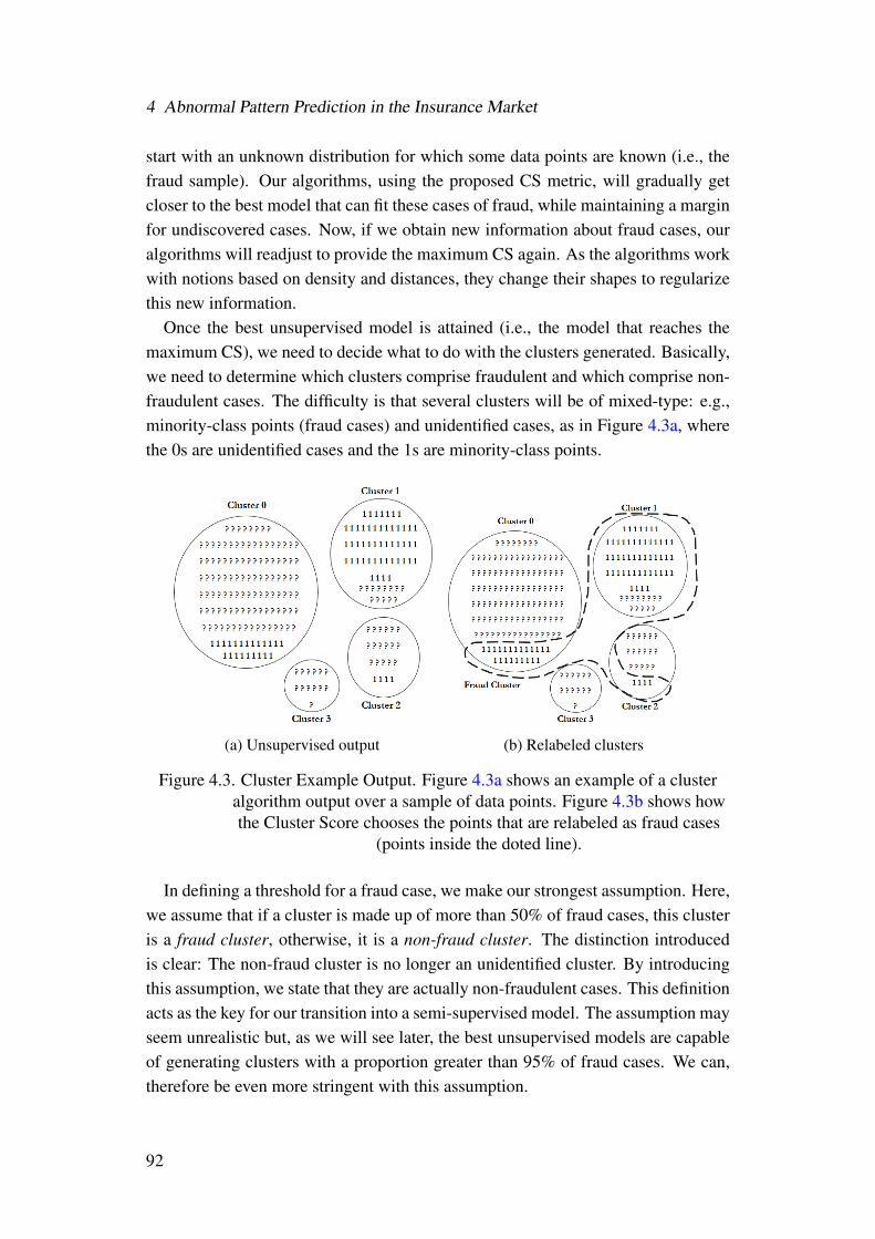
4 Abnormal Pattern Prediction in the Insurance Market
start with an unknown distribution for which some data points are known (i.e., thefraud sample). Our algorithms, using the proposed CS metric, will gradually getcloser to the best model that can fit these cases of fraud, while maintaining a marginfor undiscovered cases. Now, if we obtain new information about fraud cases, ouralgorithms will readjust to provide the maximum CS again. As the algorithms workwith notions based on density and distances, they change their shapes to regularizethis new information.
Once the best unsupervised model is attained (i.e., the model that reaches themaximum CS), we need to decide what to do with the clusters generated. Basically,we need to determine which clusters comprise fraudulent and which comprise non-fraudulent cases. The difficulty is that several clusters will be of mixed-type: e.g.,minority-class points (fraud cases) and unidentified cases, as in Figure 4.3a, wherethe 0s are unidentified cases and the 1s are minority-class points.
(a) Unsupervised output (b) Relabeled clusters
Figure 4.3. Cluster Example Output. Figure 4.3a shows an example of a clusteralgorithm output over a sample of data points. Figure 4.3b shows howthe Cluster Score chooses the points that are relabeled as fraud cases
(points inside the doted line).
In defining a threshold for a fraud case, we make our strongest assumption. Here,we assume that if a cluster is made up of more than 50% of fraud cases, this clusteris a fraud cluster, otherwise, it is a non-fraud cluster. The distinction introducedis clear: The non-fraud cluster is no longer an unidentified cluster. By introducingthis assumption, we state that they are actually non-fraudulent cases. This definitionacts as the key for our transition into a semi-supervised model. The assumption mayseem unrealistic but, as we will see later, the best unsupervised models are capableof generating clusters with a proportion greater than 95% of fraud cases. We can,therefore be even more stringent with this assumption.
92

4.3 Methodology
As Figure 4.3b shows, cluster 1, being composed of more than 50% fraud cases,now forms part of the more general fraud cluster, together, obviously, with the fraudcases already detected. The remaining cases that do not belong to such a dense fraudcluster are now considered non-fraud cases.
As mentioned, before applying the unsupervised algorithm, we had to make ahuge effort to sanitize the original data since it was collected for business purposes.This included: handling categorized data, transforming variables, bad imputation,filtering, etc. at each bottle level. Finally, we transformed the 20 bottles at a claimlevel and put them together in a unique table which formed our model’s input.
After that, before using this data as input, we made some important transforma-tions. First, we filled the missing values given that many models are unable to workwith them. There are simple ways to solve this, like using the mean or the medianvalue of the distribution. Since we did not want to modify the original distribution,we implemented a multi-output Random Forest regressor (Breiman, 2001), to pre-dict the missing values based on the other columns. The idea was, for each columnthat had missing values, we used the column as a target variable. We trained withthe part without missing values, and by using the other features, we predicted thetarget variable.
We iterated this process in every column that had missing values (0.058% of thetotal values were missing). We also measured the performance of this techniqueusing the R-squared, which is based on the residual sum of squares. Our R-squaredwas 89%.
Second, we normalized the data to, later, be able to apply a Principal ComponentAnalysis (PCA), and also because many machine-learning algorithms are sensibleto scale effects. Those using Euclidean distance are particularly sensitive to highvariation in the magnitudes of the features. In this case, we used a robust scaleapproach5 that is less affected by outliers since it uses the median value and theinterpercentile ranges (we chose 90%-10%). In general, standard normalization isa widely use method. However, as in this case we are paying special attention tooutliers, a mean approach might not be the best option. Outliers can often influencethe sample mean/variance in a negative way. The robust scale approach removesthe median and scales the data according to a quantile range. Centering and scalinghappen independently on each feature by computing the relevant statistics on thesamples in the training set. Median and interquartile range are then stored to beused on test/new data.
Third, we applied Principal Component Analysis to resolve the high dimension-ality problem (we had almost 1,300 variables). This method reduces confusion in
5We use the formulation Z = (x−xmedian)/(p90−p10)
93

4 Abnormal Pattern Prediction in the Insurance Market
the algorithms and solves any possible collinearity problems. PCA decomposesthe data-set in a set of successive orthogonal components that explain a maximumamount of the data-set’s variance. When setting a data-set’s variance threshold,a trade-off between over-fitting and getting the variation in the data-set is made.We chose a threshold of 95% (recommended threshold is between 95% and 99%),which resulted in 324 components. After this transformations, the unsupervisedalgorithm can thus be summarized as seen in Algorithm 1.
The main reason is that it has a low noise sensitivity as it ignores small variationsin the background (based on a maximum variation basis). While it is true that thereare several non-linear formulations for dimensionality reduction that may get betterresults, some studies have actually found that non-linear techniques are often not ca-pable of outperforming PCA. For instance Van Der Maaten et al. (2009) comparedPCA versus twelve non-linear dimensionality reduction techniques on several data-sets and they couldn’t conclude that the non-linear techniques outperformed PCA.
4.3.2 Supervised Model Selection
We now have a redefined target variable that we can continue working with byapplying an easy-to-handle supervised model. The first step involves re-samplingthe fraud class to avoid unbalanced sample problems. Omitting this step, meansthat our model could be affected by the distribution of classes, the reason beingthat classifiers are in general more prone to detect the majority class rather thanthe minority class. We, therefore, oversample the data-set to obtain a 50/50 bal-anced sample. We use two oversampling methods, Adaptive Synthetic SamplingApproach (ADASYN) by He et al. (2008), and balanced subsampling. ADASYNfinds the n-nearest neighbors in the minority class for each of the samples in theclass. It creates random samples from the connections and adds a random smallvalue to the points in order to scatter them and break the linear correlation with theparent point. The balanced subsample method on the other hand, does not need tocreate synthetic points since the samples used are already balanced. The balancedsamples are obtained by using weights inversely proportional to class frequenciesfor each iteration in a supervised tree based algorithm.
The second step, involves conducting a grid search and a Stratified 5-fold cross-validation (CV) based on the F-Score6 to obtain the optimal parameters for threedifferent models: extreme randomized tree -ERT- (Geurts et al., 2006), gradientboosting -GB- (Freund and Schapire, 1996) and a light XGB -LXGB- (Ke et al.,2017). Cross-validation is a great way to avoid over-fitting, i.e., failing to predictnew data. We train using k− 1 folds (data subsets) and we validate our model by
6The F-Score was constructed using β = 2, as we needed to place greater weight on the recall.
94

4.3 Methodology
Algorithm 1: Unsupervised algorithmData: Load transformed data-set. Oversample the fraud cases in order to
have the same amount as the number of unknown cases.
1 for k ∈K = {model1,model2, ...}where K is a set of unsupervisedmodels. do
2 for i ∈ I where I is a matrix of parameter vectors containing allpossible combinations of the parameters in model k do
3 We fit the model k with the parameters i to the oversampleddata-set.;
4 We get the J clusters: {C1,C2, ...,CJ} for the combination {k, i},i.e., Ck,i = {C1
k,i,C2k,i, ...,C
Jk,i};
5 For Ck,i we calculate C1 Score and C2 Score and we obtain thecluster score CSk,i, based on the acceptance threshold t∗.;
6 Save the cluster score result CSk,i ∈ CSK,I , where CSK,I is thecluster score vector for each pair {k, i}.;
7 end8 end
9 Choose the optimal CS∗ where CS∗ =max{CSK,I}
10 Relabel the fraud variable using the optimal clustering model derived fromCS∗. Each unknown case in a fraud cluster is now equal to 1, knownfraud cases are equal to 1 and remaining cases are equal to 0.
95

4 Abnormal Pattern Prediction in the Insurance Market
testing it on the remaining fold. To prevent an imbalance problem in the folds, weuse a stratified k-folds strategy which returns subsets containing approximately thesame distribution of classes as the original data-set.
We have to be careful not to over-fit the model during the cross-validation pro-cess, particularly when using oversampling methods. Step one and step two, there-fore have to be executed simultaneously. Oversampling before cross-validatingwould generate samples that are based on the total data-set. Consequently, for eachk− 1 training fold, we would include very similar instances in the remaining testfold, and vice versa. This is resolved by first, stratifying the data, and then over-sampling the k− 1 folds, without taking into account the validation fold. Finally,we concatenate all the predictions.
Additionally, we combine the supervised models using stacking models. Stack-ing models is combining different classifiers, applied to the same data-set, and get-ting different predictions that can be “stacked” up to produce one final predictionmodel. The idea is very similar to k-fold cross validation, dividing the training setinto several subsets or folds. For all k− 1 folds, predictions are obtained by usingall the supervised models (called the base models). The predictions are stored to beused as features for the stacking model in the full training data-set. Finally, a newmodel (the stacking model or the Meta model) is fitted to the improved data-set.The stacking model can discern whether a model performs well or poorly, which isvery useful since one model might have high performance when predicting fraud,but not when predicting non-fraud, and vice versa. The combination of both couldtherefore improve the results. We try three different ways of combining classifiers,modifying the Meta model: GB and LXGB with Meta ERT, GB and ERT with MetaLXGB, and LXGB and ERT with Meta GB.
Once we have the optimal parameters for each model, we calculate the optimalthreshold that defines the probability of a case being fraudulent or non-fraudulent,respectively.
Finally, we identify the two models that perform best on the data-set – the bestacting as our main model implementation, the other controlling that the predictedclaims are generally consistent. The algorithm can be summarized as seen in Algo-rithm 2.
96

4.3 Methodology
Algorithm 2: Supervised algorithmData: Load relabeled data-set.
1 for modeli ∈M ′ = {M,S} where M is the set of supervised individualmodels M and S the set of stacking models from M do
2 for {traink, testk} folds in the Stratified k-Folds do3 if Oversample==True then train′k = oversample(traink) where
oversampling is applied to 50/50 using the ADASYN method.;
4 else train′k = train′k and the balanced subsampling option isactivated.;
5 Fit the modeli in train′k, where modeli ∈M ′ = {M,S}.;
6 Get predicted probabilities pk of testk using modeli.;
7 Save the probabilities pk in Pi, where Pi is the concatenation ofmodeli’s probabilities.
8 end
9 for ∀ti ∈ [0,1], where t is a probability threshold of the modeli toconsider a case as fraudulent do
10 if Pi ≥ ti then Pi = 1;11 else Pi = 0;
12 Using Pi, where now Pi is a binary list, we calculate,FScorei,t = (1 +β2)∗ precision∗recall
recall+β2∗precision with β = 2.;
13 Save FScorei,t in FScorei, a list of vectors of modeli withFScore results for each t.
14 end15 We get FScore∗i =max{FScorei(t)}.16 end
97

4 Abnormal Pattern Prediction in the Insurance Market
4.4 Results
4.4.1 Performance
Table 4.2 shows the main unsupervised modeling results of the tuning process. Wetried different combinations of distance based models, density based models andoutlier models: Mini-Batch K-Means (Sculley, 2010), Isolation Forest (Liu, 2008),DBSCAN (Ester et al., 1996), Gaussian Mixture and Bayesian Mixture (Figueiredoand Jain, 2002). Mini-batch K-Means is not only much faster than the other mod-els, it also provides the best results. It is similar to K-Means++, both using theEuclidean distance between points as the objective function, however it can also re-duce computation time. Subsets of the input data are taken and randomly sampledin each iteration, converging more quickly to a local solution.
Model n Clusters C1 C2 CS (α = 2)
Mini-Batch K-Means 4 96.6% 96.6% 96.6%Isolation Forest 2 51.5% 51.1% 51.4%DBSCAN 2 50.2% 49.8% 50.1%Gaussian Mixture 5 95.0% 95.0% 96.3%Bayesian Mixture 6 96.5% 96.4% 96.5%
Table 4.2. Unsupervised model results
C1 indicates that the minority-class (fraud) clusters comprise approximately 96.59%of minority data points on a weighted average. In contrast, C2 indicates they aremade up of 96.59% of unknown cases. As can be seen in Table 4.3, more than95% of the cases in the central cluster are fraudulent (well above our 50% assumedthreshold), but it also contains an additional 6,047 unknown cases (Cluster 0 nowcontains an additional 5,890 cases, and Cluster 1 an additional 157 cases). This isour core fraud cluster and the one we use when renaming the original labels.
After relabeling the target variable (with the Mini-Batch K-Means output), wecalculate the supervised models performance using Stratified 5-Fold CV on the data-set. The results of each of the supervised models and of the stacking models isshown in Table 4.4.
As can be appreciated, we have two recall values. The cluster recall is the metricderived when using the relabeling target variable. The original recall emerges whenwe recover the prior labeling (1 if it was fraud, 0 otherwise). As can be seen, theresults are strikingly consistent. We are able to predict fraud cluster with a recall ofup to 89-97% in every case. But, more impressively yet, we can capture the originalfraud cases with a recall close to 98%. The precision is slightly lower, but in almost
98

4.4 Results
Clusters Fraud Percentage
0 0 2%0 1 98%1 0 99%1 1 1%2 0 100%2 1 0%3 0 1%3 1 99%
Table 4.3. Oversampled Unsupervised Mini-Batch K-Means
all cases it is higher than 67%. These are particularly good results for a problem thatbegan as an unsupervised high-dimensional problem with an extremely unbalanceddata-set.
Model Cluster Recall Original Recall Precision F-Score
ERT-ss 0.9734 0.9840 0.6718 0.8932ERT-os 0.9647 0.9819 0.6937 0.8948GB 0.9092 0.9376 0.6350 0.8369LXGB 0.8901 0.9249 0.7484 0.8576Stacked-ERT 0.8901 0.9283 0.7524 0.8587Stacked-GB 0.8947 0.9287 0.7630 0.8649Stacked-LXGB 0.9180 0.9464 0.6825 0.8588
Table 4.4. Supervised model results
The two best models are both extreme randomized trees: the first uses balancedsubsampling -ERT-ss- (i.e., for every random sample used during the iteration ofthe trees, the sample is balanced by using weights inversely proportional to classfrequencies), and serves here as our base model; the second uses an ADASYNoversampling method-ERT-os- and serves as our control model.
4.4.2 Investigation Office Validation
At the outset, we randomly set aside 10% of the data (30,317 claims). In this finalstep, we want to go further and examine these initial claims as test data. Our resultsare shown in Table 4.5.
As can be appreciated, the control model (Table 4.5b) has a recall of 97% whilethe base model (Table 4.5a) has an impressive recall of 100%. However, the real
99

4 Abnormal Pattern Prediction in the Insurance Market
Original Value Prediction Cases
NON-INVESTIGATED NON-FRAUD 29.631FRAUD NON-FRAUD 0
NON-INVESTIGATED FRAUD 415FRAUD FRAUD 271
(a) ERT-ss Robustness Check.
Original Value Prediction Cases
NON-INVESTIGATED NON-FRAUD 29.656FRAUD NON-FRAUD 8
NON-INVESTIGATED FRAUD 390FRAUD FRAUD 263
(b) ERT-os Robustness Check.
Table 4.5. Model Robustness Check.
added value depends on the non-investigated fraud cases, i.e., cases not previ-ously detected but which would boost our results if shown to be fraudulent (non-investigated predicted as fraud). We, therefore, sent these cases to the IO for analy-sis.
The IO investigated 367 cases (at the intersection between the ERT-ss and ERT-osmodels). Two fraud investigators analyzed each of these cases, none of which theyhad previously seen as the rule model had not detected them.
Of these 367 cases, 333 were found to present a very high probability of be-ing fraudulent. This means that only 34 could be ruled out as not being fraudulent.Recall that from the original sample of 415 cases, the fact that 333 presented indica-tions of fraud means we have a precision of 88%. In short, we managed to increasethe efficiency of fraud detection by 122.8%. These final outcomes are summarizedin Table 4.6.
Original Value Prediction Cases
NON-INVESTIGATED NON-FRAUD 29.631FRAUD NON-FRAUD 0
NON-FRAUD FRAUD (415 - 333) = 82FRAUD FRAUD (271 + 333) = 604
Table 4.6. Base Model Final Results
4.4.3 Dynamic Learning
One of the challenges in fraud detection is that it is a dynamic process which canchange its patterns over time. A year later, we retest the model with new data. Wenow have 519,921 claims to evaluate. We initially start out with a similar proportionof fraud cases (0.88%)- we are now able to train with 4,623 fraud cases to furtherimprove results.
First, we recalculate the unsupervised algorithm, getting a Cluster-Score of 96.89%.As can be seen in Table 4.7, Cluster 0 contains almost every normal case. On
100

4.5 Conclusion
the other hand, we can clearly distinguish two fraud clusters: Cluster 1, in which99.31% are fraud cases, and Cluster 2, in which 97.36% are fraud cases. Our 50%threshold therefore becomes insignificant again.
Clusters Fraud Percentage
0 0 99.4%0 1 0.6%1 0 0.7%1 1 99.3%2 0 2.6%2 1 97.4%
Table 4.7. Oversampled Unsupervised Mini-Batch K-Means
Using the Extreme Randomized Subsampled approach (ERT-ss) and the ExtremeRandomized oversampled with ADASYN (ERT-os), and the Stratified 5-fold crossvalidation approach we retrain the model. Table 4.8 shows the main results.
PERIOD Jan15-Jan17 Jan15-Jan18
Claims 303,166 519,921Observed Fraud 2,641 4,623Cluster Score 96.59% 96.89%Recall Score ERT-ss 97.34% 96.31%Precision Score ERT-ss 67.18% 89.35%F-Score ERT-ss 89.32% 94.84%Recall Score ERT-os 96.47% 96.44%Precision Score ERT-os 69.37% 92.18%F-Score ERT-os 89.48% 95.56%
Table 4.8. Base Model with the machine-learning process applied
The base model greatly improves the homogeneity of the fraud and non-fraudclusters. In particular, it provides a gain of 33% in the precision score and of 6.2-6.8% in the F-Score.
4.5 Conclusion
This chapter has sought to offer a solution to the problems that arise when workingwith highly unbalanced data-sets for which the labeling of the majority of cases isunknown. In such cases, we may dispose of a few small samples that contain highlyvaluable information. Here, we have presented a fraud detection case, drawing on
101

4 Abnormal Pattern Prediction in the Insurance Market
the data provided by a leading insurance company, and have tested a new methodol-ogy based on semi-supervised fundamentals to predict fraudulent property claims.
At the outset, the Investigation Office (IO) did not investigate many cases (around7,000 cases from a total of 303,166). Of these, only 2,641 were actually true posi-tives (0.8% of total claims), with a success rate of 48%. Thanks to the methodologydevised herein, which continuously readapts to dynamic and changing patterns, wecan now investigate the whole spectrum of cases automatically, obtaining a totalrecall of 96% and a precision of 89-92%. In spite of the complexity of the initialproblem, where the challenge was to detect fraud dynamically without knowinganything about 99.2% of the sample, the methodology described has been shown tobe capable of solving the problem with great success.
4.6 Appendix. Practical Example
Imagine we have the following output from an unsupervised model:
Class Label
0 10 20 30 11 21 21 30 30 30 20 10 31 20 11 2
Table 4.9. Class and Labels
The classes represent fraud (=1) and unlabeled (=0). The output label is theclustering label. As can be seen, just 33% of cases represent detected fraud. If wegroup the class by clusters:
102

4.6 Appendix. Practical Example
Label Class Subtotal Class Total
1 0 4 41 1 0 42 0 2 62 1 4 63 0 4 53 1 1 5
Table 4.10. Grouping Labels and Classes
As is evident, the fraud class tends to be assigned to the second cluster.First we calculate C1.
C1 =04 ∗0 + 4
6 ∗4 + 15 ∗1
5= 0.5733
Then we calculate C2 using a similar formula.
C2 =44 ∗4 + 2
6 ∗2 + 45 ∗4
10= 0.7867
As can be seen, C1 gives worst results as its core group (group 2) is quite con-taminated (66% of observations actually correspond to cases of fraud). This effectrepresents 93% of the total effect. The effect of mismatching the core group (1/5)is negligible, which stresses the importance of constructing a strong core group.
This conclusion is notorious in the case of C2. Non-identified classes are highlyrobust in two groups (1 and 3).
If we calculate the CS with α = 2 (balanced C1 and C2) we obtain:
CS = 0.6062
which is a value very close to 0.5733. This formula allows us to balance our results,giving greater weight to the lower score. We should stress we want both good andbalanced scores; thus, C1=0, C2=1 is not the same as C1=0.5, C2=0.5. Indeed, theformer returns a CS=0. We compare the mean with the CS in Table 4.11.
103

4 Abnormal Pattern Prediction in the Insurance Market
C1 C2 Mean CS
0.0 1.0 0.5 0.000.1 0.9 0.5 0.180.2 0.8 0.5 0.320.3 0.7 0.5 0.420.4 0.6 0.5 0.480.5 0.5 0.5 0.500.6 0.4 0.5 0.480.7 0.3 0.5 0.420.8 0.2 0.5 0.320.9 0.1 0.5 0.181.0 0.0 0.5 0.00
Table 4.11. C1 and C2 Combinations
As can be seen, we obtain the same unbalanced scores as the balanced outcomesfor the mean score. CS penalizes the unbalanced scores. This is why we obtaindifferent results with the same proportions.
However, we can make adjustments in terms of the relevance we attach to eachgroup. If we raise α, we penalize the C2 results, and vice versa.
What happens if we choose α≥ 2?
C1 C2 α = 2 α = 4 α = 6
0.1 0.9 0.12 0.11 0.100.2 0.8 0.24 0.21 0.200.3 0.7 0.34 0.31 0.300.4 0.6 0.43 0.41 0.400.5 0.5 0.50 0.50 0.500.6 0.4 0.55 0.58 0.590.7 0.3 0.55 0.65 0.680.8 0.2 0.50 0.68 0.740.9 0.1 0.35 0.61 0.74
Table 4.12. C1 and C2 Combinations with α≥ 2
As is evident, we obtain two effects. First, while C1 increases, CS also increases(although C2 decreases at the same rate). But the effect present in the balanced casenow extends further. When we are at C1=0.7, the balanced effect tends to reverse
104

4.6 Appendix. Practical Example
the situation or to slow the increasing rate. The second effect is that the score curvetends to a linear curve while we increase α. CS is now depending more strongly onC1 being higher; while the higher α the stronger C1.
105

5 Risk Categorization andSelf-Reported Mechanisms inAutomobile Insurance Markets
5.1 Introduction
In automobile insurance markets, companies face a severe problem of asymmetricalinformation during the underwriting process: they know next to nothing about theirpotential new customers, while the latter might tend to underreport prior claimswhen switching to a new company. In these markets, risk classification is generallyexplained by adverse selection which is a result of asymmetric information betweeninsured and insurers. The insured are a heterogeneous group that has more informa-tion than the insurer, who is unable to differentiate between risk types. Indeed, it isa costly process for the company to detect who the high risk individuals are, and thelatter have no incentives to reveal their true nature. This results in risk pooling (Ar-row, 1963), which is necessarily inefficient as it averages the price between the low-and high-risk insured (Akerlof, 1970). There is a chance that the costs and claimswill be higher than the premium paid by the customer. The opposite is to overratethe premium, and thereby becoming noncompetitive in the market and reducing thefirm’s amount of customers.
In one period contracts, basic insurance theory suggests that risky customers willnot reveal their true nature and, therefore, a suboptimal Pareto equilibrium withan average premium will be reached if no additional incentives are imposed (seeRothschild and Stiglitz, 1976; Stiglitz, 1977). In this chapter we seek to addressthe following questions: Are all “bad risks” pretending to be “good risks” as insur-ance theory suggests? Or is it more nuanced, in that only a subset misreport theirhistory? How relevant is “misreporting” in predicting risk, i.e. are “misreporters”particularly risky? And, is there any insight into what type of consumers are likelyto misreport? Using self-reported data and observable data on potential customersfrom a leading insurance company in Spain, we find that combining self-reporteddata with observable characteristics allow us to reach an equilibrium that is close to
107

5 Risk Categorization and Self-Reported Mechanisms in Automobile Insurance Markets
the public information equilibrium.The first and most common mechanism to reduce asymmetry information is the
self-selection mechanism: Insureds with different risk types self-select themselvesamong a menu of policies offered by the insurers. The result is a Pareto im-provement compared to the single contract solution with an average premium (seeCrocker and Snow, 2000). Based on the hypothesis that the high-risk individualsopt for higher coverage, empirical literature have evaluated conditional correlationsbetween insurance coverage and subscribers’ ex-post risk. The issue with this cor-relation, however, is that it fails to address the problem of unobserved data, as re-vealed ex-post the subscription process. Even though we assume that the coverageis a proxy of the policyholders’ risk, there are additional unobserved differencesamong the insured (e.g., risk aversion, precaution levels, etc.). Furthermore, thefact that there is a correlation between coverage and risk does not mean that ad-verse selection is assured as it might also reflect moral hazard (which could nullifythe effect). Finally, this correlation is not always conclusive (Dahlby, 1983, 1992;Chiappori and Salanié, 2000; Saito, 2006).
A second well-known mechanism is risk categorization which is based on vari-ables that are costless to observe and are correlated with the unobservable risk ofloss. For example, age, gender, type of car, etc. In this case, Pareto improvementsare obtained by using imperfect signals to categorize risks (Hoy, 1982; Crocker andSnow, 1986). A well-known example is Dionne and Vanasse (1992) who find thatyoung male drivers are riskier than young female drivers, using data from Quebecautomobile drivers. However, this mechanism may generate an unfair price to theinsured driver as it is based on imperfect signals. Several authors have mentionedthis issue of underwriting and uncertainty. As early as 1982, de Wit pointed out thatthe process of setting the premium in non-life insurance was much harder due tothe fact that using external data or shared company data is not always possible. Theinsured premium is therefore calculated only by available and measurable factors.In the end, what usually happens is that companies rely on simple judgment or de-cision rules. Even more, as mentioned by Kunreuther et al. (1995), the pricing risktends to be higher in the existence of ambiguity about the probability of events. It isvery common that private information, hidden within the applicant pool (high-riskobservables as age, license years, etc.), explains a great part of the rejections.
However, if we assume that not all risky potential customers misreport as in-surance theory suggests, we could combine this information with the traditionalrisk categorization method to solve its inefficiencies when predicting risky potentialcustomers. Our main objective in this chapter is, therefore, to theoretically and em-pirically evaluate the combination of risk categorization tools and self-reported datain predicting risky customers ex-ante the policy is signed. Ideally, companies would
108
5.1 Introduction
want to know new customers’ unobserved characteristics (such as their past perfor-mance in other companies, reliability, etc.) to be able to detect high-risk customersand to distinguish them from those with good records. As we are usually unableto know the past behavior of a new customer, we propose mixing two mechanisms:First, observable data from the potential new customer and historical data from theinternal customers as a proxy of the unknown characteristics; second, self-reporteddata about past performance behavior.
The Spanish insurance market offers us a good opportunity to evaluate the ques-tions mentioned earlier and the ability to predict risky customers. Leading compa-nies subscribe to a private service where they can share historical data about cus-tomers. Thus, when a new customer switches to another company, prior claims canbe checked. The data comprises responses to only a few questions, but they are veryprecise. Specifically, they provide information about the number of years as insuredand the number of previous claims. We can then use this information as validationof our methodology. Additionally, in the underwriting process, the policies that areoffered are based, in part, on the responses to a number of questions by potentialnew customers. These questions also refer to years as insured and previous perfor-mance. If people were always to tell the truth about their own risk (i.e. revealingunobserved characteristics), it would be easy to set a fair price. As we observe be-low, only a very small number of people misreport (5.5% in our data-set), whilethose that lie increase the premiums offered to the truthful and, in some cases, thismight even deter them from contracting with said company.
In doing so, we propose a new methodology for predicting risk. As companieshave little information about new customers (but a considerable amount about theirown), and only a small percentage lie about their true risk status, we show belowthat we can reduce the asymmetric information problem to one of anomaly detec-tion. To do so, we propose applying deep variational autoencoder (VAE) models,that is, representations of neural networks, based on the idea of compressing and de-compressing data. VAE models learn from a compressed representation of the dataand from the latent variables obtained from the input. We expect the VAE model tominimize the asymmetric information problem by using a database containing onlyobservables about new customers and internal customer data. In this way we seekto construct a model that can detect anomalies during the underwriting process and,thus, allow a fair price to be set as underreported claims should have been detected.
We conclude that combining self-reported data with risk categorization leads totwo main outcomes: First, we are capable of predicting riskier customers ex-antethe policy is subscribed, something which we are not capable of when using onlyobservable data. Second, we show that the most influential variables accounting foradverse selection are self-reported years as insured, cluster constructed variables
109

5 Risk Categorization and Self-Reported Mechanisms in Automobile Insurance Markets
related to customers’ zip code and characteristics, if the insured was the owner andfirst driver in the policy, if the insured’s age was higher than 65, if the customerwas male or female and the number of license years. The evidence we present issupported by empirical findings, which reveal that a great proportion of high riskindividuals do not misreport their risk nature. Additionally, we present a theoreticalmodel which helps explaining how combining self-reported data with risk catego-rization improves the potential profit for the insurer monopoly.
5.2 Literature Review
There is a vast literature on asymmetric information in insurance markets that hasbeen strongly influenced by contract theory (Rothschild and Stiglitz, 1976; Stiglitz,1977; Wilson, 1977; Miyazaki, 1977; Spence, 1978; Hoy, 1982; Kunreuther andPauly, 1985; Dionne and Lasserre, 1985, 1987; Hellwig, 1986, Cooper and Hayes,1987; Hosios and Peters, 1989; Nilssen, 2000; Dionne, 1992; Dionne and Do-herty, 1994; Fombaron, 1997, 2000; Crocker and Snow, 1985, 1986, 2013). Severalmechanisms have been proposed to reduce the inefficiency associated with adverseselection. The first and most common is the self-selection mechanism, where in-sureds with different risk types self-select themselves among a menu of policiesoffered by the insurers. The result is a Pareto improvement compared to the singlecontract solution with an average premium.
With the increasing availability of data (especially, in insurance companies), em-pirical evidence of adverse selection has acquired relevance. Several studies haveevaluated conditional correlations between insurance coverage and subscribers’ ex-post risk, based on the hypothesis that the high-risk insured opt for higher cover-age. Thus, many authors report a positive correlation between risk and coverage(Brugiavini, 1993; Puelz and Snow, 1994; Chiappori, 1994; Dionne et al., 1999;Philipson and Cawley, 1999; Richaudeau, 1999; Dionne et al., 2000; Cardon andHendel, 2001, Chippori et al., 2002; Finkelstein and Poterba, 2002, 2004; Davidoffand Welke, 2004; Cohen, 2005; Finkelstein and McGarry, 2006; Chiappori et al.,2006; He, 2009; Einav et al., 2010; Cohen and Siegelman, 2010).
A second type of mechanisms proposed to solve this resource allocation problemrelies on multi-period contracts theory. Long-term contracting adjust ex-post in-surance premiums or coverage to past behavior. Several studies have discussed thestatic notion of asymmetric information and introduce the notion of dynamic datato handle the issue of asymmetric learning (Abbring et al., 2003a, 2003b). Basedon historical claims data, we can expect a positive correlation between past and fu-
110

5.2 Literature Review
ture claims, which reveals the policyholder’s risk type1. Both insured and insurermay garner information about a policyholder’s risk type. Hendel and Lizzeri (2003)find strong evidence of dynamic learning based on long-term contracts with a com-mitment to renew. Finkelstein et al. (2005) and Finkelstein and McGarry (2006)provide support for this evidence by using data on long-term care insurance. Fur-thermore, the learning process may not be symmetrical, and the policyholder cangain an advantage over the insurer. For instance, Cohen (2005) reports a positivecorrelation between coverage and risk for new customers with three or more yearsof driving experience, but finds no-correlation amongst new customers with lessexperience.
However, dynamic learning can only solve the lack of information problem ex-post the contract is signed, i.e., companies have to wait until policy renewal toresolve the problem. Additionally, companies are reticent to share past informa-tion about their own customers. Given that new customers tend to underreportprior claims when switching to a new insurer, each insurance company does infact have an informational advantage over other companies as regards repeat cus-tomers. However, as D’Arcy and Doherty (1990) point out, insurance companiesdo not allow intermediaries to sell private information about their customers, andso by retaining information hold on to their market power. This practice has alsobeen studied by Cohen (2008) who finds evidence consistent with insurance com-panies retaining private information about repeat customers. She demonstrates thatcompanies obtain higher profits from repeat customers who have good records, andthat these profits rise the longer the customer remains with the company. Duringthe course of a contract, a customer’s risk level may be revealed and this enhancedability to determine an appropriate premium risk should result in higher profits.In this way, companies can discriminate their prices so that, eventually, customerswith good records stay and those with bad records switch to another company. Theproblem remains, however, insofar as the company to which a customer is switch-ing does not have this information and cannot, therefore, distinguish between thosewith bad records and those that switch due to exogenous factors.
A third type of mechanisms are those related with categorization of risks. Inthis case, Pareto improvements are obtained by using imperfect signals to catego-rize risks. Hoy (1982) is the first to theoretically analyze the effect of risk catego-rization in the market equilibrium, however, his conclusions about the usefulness ofthe method are ambiguous. Crocker and Snow (1986) compare utility-possibilityfrontiers with and without risk categorization, and they find that prior categoriza-tion results in a Pareto improvement below a specific threshold. Empirically, private
1Other relevant studies are Israel (2004) and Dionne et al. (2013).
111

5 Risk Categorization and Self-Reported Mechanisms in Automobile Insurance Markets
information and rejections in insurance was studied by several authors. High-riskobservable characteristics are usually applied by insurers to deter potential high-riskinsureds. Murtaugh et al. (1995), in long-term care insurance, estimate that between12-23% of potential customers would be rejected if everyone applied at the age of65 (20-31% if applied at 75). Hendren (2013) reports that between 2007 and 2009,1 in 7 applicants to the four largest health insurance companies in the United Stateswere rejected, and shows how the existence of private risk information implied thatinsurance companies rejected people only based on observables (for three differenthealth insurance markets). There is a vast literature that relates risk classificationand observable characteristics. Puelz and Kemmsies (1993), Lemaire (1995) andDoerpinhaus et al. (2008) evaluate the impact of gender and other demographicvariables on premium pricing. Age and risk classification is another well-studiedrelation (Brown et al., 2007; Braver and Trempel, 2004; Tefft, 2008). Dionne andVanasse (1992) find strong evidence between risk and young males, and also be-tween risk and classes of driver’s license.
Several authors propose different classification systems to classify risk in insur-ance: statistical measures (Tryfos, 1980; Freifelder, 1985; Lemaire, 1985; Samson,1986; Dionne and Vanasse, 1992), linear models (Samson and Thomas, 1987; Ohls-son and Johansson, 2010; Bortoluzzo et al., 2011; David, 2015), clustering tech-niques (Williams and Huang, 1997; Smith et al., 2000; Yeo et al., 2001). However,these kinds of models have several limitations regarding: solving non-linear rela-tions, the existence of too many variables, and high dispersion (which is quite com-mon for insurance databases). A few recent studies have started to apply machine-learning and data mining techniques to claims and risk (Gepp et al., 2012; Guelman,2012; Liu et al., 2014; Yang et al., 2015; Kašcelan et al., 2015). In our case, we pro-pose using a deep Variational Autoencoder approach. Autoencoder networks havetraditionally been used in image classification (Tan et al., 2010; Krizhevsky andHinton, 2011; Hinton et al., 2011; Walker et al., 2016; Pu et al., 2016; Theis et al.,2017); however, they have recently been used more frequently with structure data,especially in relation to anomaly detection problems (Dau and Song, 2014; An andCho, 2015; Andrews et al., 2016; Zhai et al., 2016; L. Paula et al., 2016; Zhou andPaffenroth, 2017; Cozzolino and Verdoliva, 2017; D’Avino et al., 2017; Schreyeret al., 2017). The main advantages of using variational autoencoder networks are:Firstly, they can reduce data to their true nature, cleansing them of any undesiredfeatures and noise. Here, we have a large data-set containing many variables aboutinternal customers, but as we do not know which are relevant for predicting risky po-tential customers, VAE should be able to help us address this problem. It works byreducing the number of nodes through hidden layers, so that we can extract the ac-tual features representing the data. Secondly, existing outlier detection approaches
112

5.3 Theoretical Model
are usually based on notions of distance and density, meaning they work in the orig-inal data’s space. As a result, they tend to underperform when applied to nonlinearstructures. To solve this issue, a deep autoencoder model can be transformed into apowerful semi-supervised outlier detection model.
5.3 Theoretical Model
The model developed by Rothschild and Stiglitz (1976) and further elaborated byStiglitz (1977) introduces a risk neutral private monopoly that offers insurance cov-erage (βi) for an insurance premium (αi) in a single-period contract and under pub-lic information. For simplicity, there are three types of risk (i ∈ {L,M,H}). Ini-tially, we assume that risk type H and M have the exact same level of risk. Thus,pH = pM > pL. Each insured owns a risky asset with monetary value D(x) whichdepends on two possible states of the world x ∈ {n,a}: a represents the accidentstate with probability pi, and n represents the no accident state with probability1−pi, such that D(a) = 0 in state a and D(n) =D in state n.
The expected utility of the insured under the contract Ci = {αi,βi} and initialwealth W0, is equal to:
V (Ci|pi) = piU(W0−D−βi) + (1−pi)U(W0−αi)
which is strictly concave and satisfies the von Neumann-Morgenstern axioms2.Therefore, with public information and without transaction cost, the problem canbe summarized as:
maxαi,βi,λi
∑qi[(1−pi)αi−piβi]
Subject to the participating constraint V (Ci|pi)≥ V 0i (the monopoly can extract
all the consumer surplus). In presence of public information about insureds’ risk, itcan be proved that insureds get full insurance coverage (β∗i =D−α∗i ), that there isno consumer surplus, and that αL < αM = αH . We illustrate this solution in Figure5.1. As the monopoly can distinguish between insureds, it offers one of three con-tracts: {C∗L,C∗M ,C∗H} to which insureds are indifferent between the offered contractand the self-insurance contract C0.
Hereinafter, we assume the existence of private information about insureds’ risktypes. Theory suggests that if the monopoly offers the same contract to differentrisk types, it is rational for both, H and M , to move to a contract CL and, theconsequence is a pooled equilibrium where the monopoly cannot distinguish among
2U ′ > 0, U ′′ < 0.
113
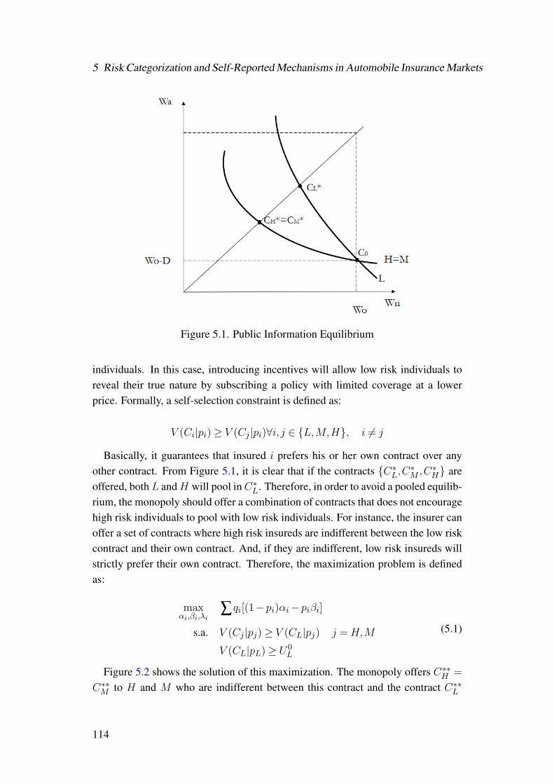
5 Risk Categorization and Self-Reported Mechanisms in Automobile Insurance Markets
Figure 5.1. Public Information Equilibrium
individuals. In this case, introducing incentives will allow low risk individuals toreveal their true nature by subscribing a policy with limited coverage at a lowerprice. Formally, a self-selection constraint is defined as:
V (Ci|pi)≥ V (Cj |pi)∀i, j ∈ {L,M,H}, i 6= j
Basically, it guarantees that insured i prefers his or her own contract over anyother contract. From Figure 5.1, it is clear that if the contracts {C∗L,C∗M ,C∗H} areoffered, both L andH will pool inC∗L. Therefore, in order to avoid a pooled equilib-rium, the monopoly should offer a combination of contracts that does not encouragehigh risk individuals to pool with low risk individuals. For instance, the insurer canoffer a set of contracts where high risk insureds are indifferent between the low riskcontract and their own contract. And, if they are indifferent, low risk insureds willstrictly prefer their own contract. Therefore, the maximization problem is definedas:
maxαi,βi,λi
∑qi[(1−pi)αi−piβi]
s.a. V (Cj |pj)≥ V (CL|pj) j =H,M
V (CL|pL)≥ U0L
(5.1)
Figure 5.2 shows the solution of this maximization. The monopoly offers C∗∗H =
C∗∗M to H and M who are indifferent between this contract and the contract C∗∗L
114
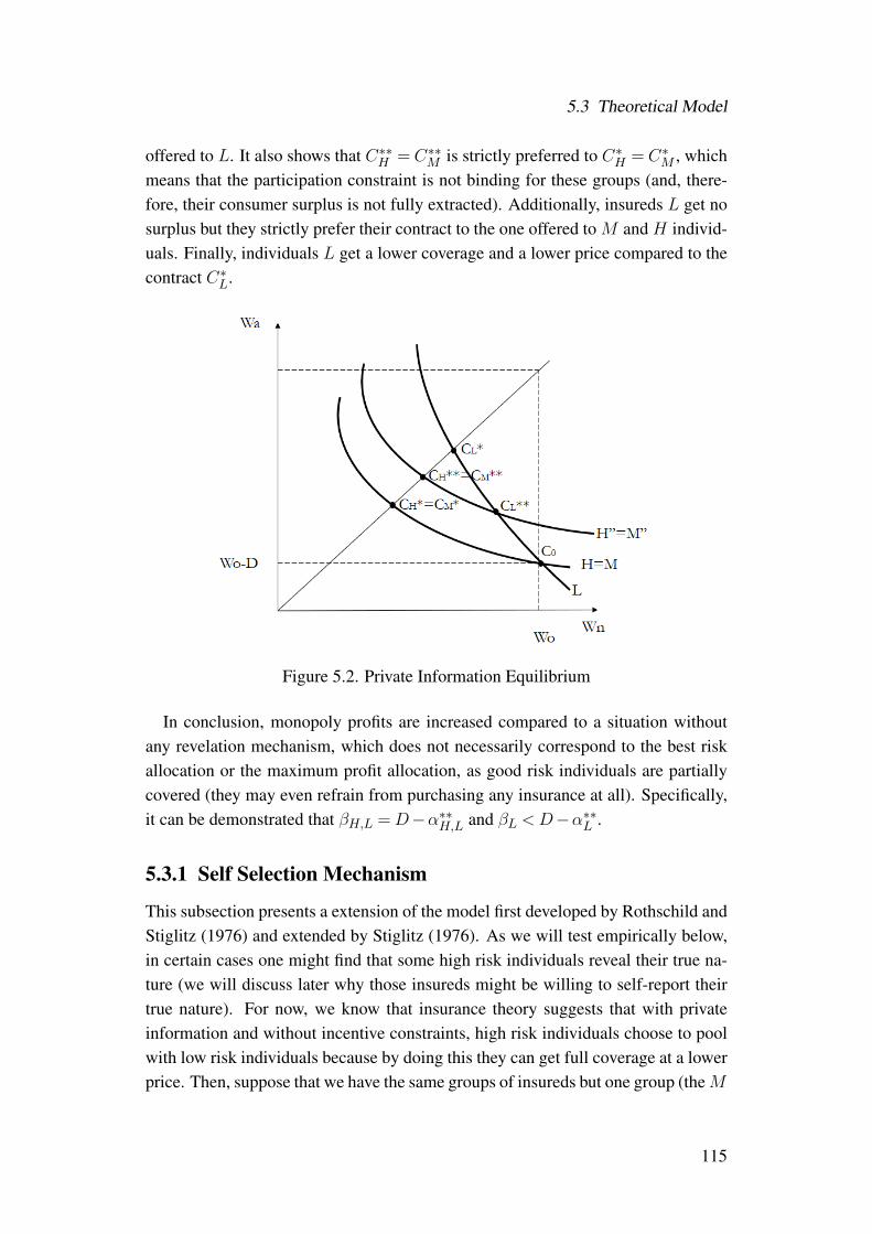
5.3 Theoretical Model
offered to L. It also shows that C∗∗H = C∗∗M is strictly preferred to C∗H = C∗M , whichmeans that the participation constraint is not binding for these groups (and, there-fore, their consumer surplus is not fully extracted). Additionally, insureds L get nosurplus but they strictly prefer their contract to the one offered to M and H individ-uals. Finally, individuals L get a lower coverage and a lower price compared to thecontract C∗L.
Figure 5.2. Private Information Equilibrium
In conclusion, monopoly profits are increased compared to a situation withoutany revelation mechanism, which does not necessarily correspond to the best riskallocation or the maximum profit allocation, as good risk individuals are partiallycovered (they may even refrain from purchasing any insurance at all). Specifically,it can be demonstrated that βH,L =D−α∗∗H,L and βL <D−α∗∗L .
5.3.1 Self Selection Mechanism
This subsection presents a extension of the model first developed by Rothschild andStiglitz (1976) and extended by Stiglitz (1976). As we will test empirically below,in certain cases one might find that some high risk individuals reveal their true na-ture (we will discuss later why those insureds might be willing to self-report theirtrue nature). For now, we know that insurance theory suggests that with privateinformation and without incentive constraints, high risk individuals choose to poolwith low risk individuals because by doing this they can get full coverage at a lowerprice. Then, suppose that we have the same groups of insureds but one group (theM
115

5 Risk Categorization and Self-Reported Mechanisms in Automobile Insurance Markets
insureds), for some reason (idiosyncratic reasons, fear to future penalization, differ-ences in risk aversion, etc.), reveals its true nature and, therefore, the monopoly haspublic information about it. In this case, the monopoly can increase its benefits byoffering a new contract to which this group is indifferent between the new contractand self-insurance (see Figure 5.3).
Figure 5.3. Semi-Private Information Equilibrium
In this situation, the monopoly must still separate between H and L and, thus,the maximization profit problem can be defined as:
maxαi,βi,λi
∑qi[(1−pi)αi−piβi]
s.a. V (Cj |pj)≥ V (CL|pj) j =H,M
V (CL|pL)≥ U0L
(5.2)
Proposition 1. In the presence of semi-private information, i.e., a situation wherethe monopoly knows the nature of some high-risk individuals (e.g., insuredsM ), theoptimal one-period contract equilibrium has the following characteristics:
• The monopoly offers CM∗ such that individuals M have no consumer sur-plus: V (C∗M |pM ) = V 0
M .
• The monopoly offers C∗∗L to insureds L and it also extracts the consumersurplus: V (C∗∗L |pL) = V 0
L .
116
5.3 Theoretical Model
• Insureds H strictly prefer C∗∗H to CM∗ and they are indifferent between C∗∗Land C∗∗H . Consumer surplus is positive: V (C∗∗H |pH)> V H
0 .
• Both, H and M get full coverage equal to β∗∗H =D−α∗∗H and β∗M =D−α∗M .Individuals L get partial coverage (or no coverage) at a lower price, moreprecisely, β∗∗L < β∗∗H < β∗M and α∗∗L < α∗∗H < α∗M .
• The monopoly profit is in this case higher than in the full private infor-mation equilibrium but lower than in the public information equilibrium:π(C∗∗L ,C
∗∗M ,C
∗∗H )< π(C∗∗L ,C
∗M ,C
∗∗H )< π(C∗L,C
∗M ,C
∗H).
In conclusion, the monopoly increases the profits compared to the private infor-mation case. However, partial coverage (and even no coverage) and offering a lowerprice to low risk individuals is still necessary to separate between high and low riskindividuals.
5.3.2 Risk Categorization
The monopoly can combine information from some of the high risk individuals thathave revealed their true nature and a risk categorization mechanism to separate highrisk individuals from low risk individuals. The risk categorization theory suggeststhat imperfect information such as observable characteristics can be used to obtainPareto improvements for resource allocation (Hoy, 1982; Crocker and Snow, 1986).
Suppose for example that we have derived two possible groups from the observ-able characteristics of self-selected insureds. Then, we assume that insureds differin characteristics that are costless to observe and which are also correlated with theunobservable risk. By using this information, we separate between: Group A witha proportion of high risk individuals wAH and low risk individuals wAL , and group Bwith a proportion of high risk individuals wBH and low risk individuals wBL . The ob-servable characteristics determine the proportion of high risk individuals is higherin the group A than in the group B, that is, wBH >wAH and wAL >wBL (wBH = 1−wBLand wAH = 1−wAL ). Bearing this in mind, we derive the proposition below. For sim-plicity, we add a group C in which we know all individuals are type M individuals.The size of each group is defined as: qL, qM and qH , respectively.
Proposition 2. In the presence of semi-private information, it is possible to reachthe Pareto optimal equilibrium under perfect information if there are characteristicsthat are costless to observe and which correlate perfectly with the unobservable riskof loss.
To demonstrate this, we first define the profit definition under perfect information:
117
5 Risk Categorization and Self-Reported Mechanisms in Automobile Insurance Markets
pi∗ = qLπ(C∗L|pL) + qMπ(C∗M |pM ) + qHπC∗H |pH)
If the monopoly knows that the characteristics are highly correlated with the risk,then it can offer groupA (with a high proportion of low risk individuals) the contractoffered to L in the perfect information case (C∗L), and it can offer group B contractC∗H . Thus, the profits with risk categorization and self-reported risk can be formallydefined as:
πRC = qA[wAHπ(C∗L|pH) + (1−wAH)π(C∗L|pL)]+
qB[wBHπ(C∗H |ph) + (1−wBH)π(C∗H |pL)] + qCπ(C∗M |pM )(5.3)
If the categorization is accurate: wAH→ 0, wBH→ 1, qA→ qL and qB→ qH . Then,we can conclude that:
πRC → π∗
Proposition 3. In the presence of semi-private information, there exist equilibriain which the monopoly can get higher profits than the private information equi-librium (but strictly lower than the perfect information equilibrium), if there areobservable characteristics that are costless to observe and which do not correlateperfectly with the unobservable risk of loss. The stability of these equilibria finallydepend on to which extent the risk categorization tool correlates with the risk.
If the monopoly offers group A contract C∗L, group B contract C∗H and group Ccontract C∗M , the monopoly profit can be defined as:
πCR = qA(1−wAH)π(C∗L|pL) + qB(1−wBH)π(C∗H |pL)+
qAwAHπ(C∗L|pH) + qBw
BHπ(C∗H |pH) + qCπ(C∗M |pM )
(5.4)
However, if the signal is imperfectly informative, then, some L individuals areoffered C∗H . Thus, the participation constraint is violated because at this particularutility level, L does not participate. As a result, π(C∗H |pL) = 0, which impliesthat without a perfect signal, profits are strictly lower than the profits under perfectinformation.
We now focus on the next part of the proposition. That is, if there exist equilibriawhere imperfect information allows the monopoly to get higher benefits than withprivate information. That is:
πCR ≥ π∗∗
Which is equivalent to:
118

5.3 Theoretical Model
πRC = qA(1−wAH)[(1−pL)α∗L−pLβ∗L]
+ qAwAH [(1−pL)α∗L−pHβ∗L]
+ qBwBH [(1−pH)α∗H −pHβH∗]
+qM [(1−pM )α∗M −pMβ∗M ]≥π∗ = qL[(1−pL)α∗∗L −pLβ∗∗L ]
+ qM [(1−pM )α∗M −pMβ∗M ]
qH [(1−pH)α∗∗H −pHβ∗∗H
(5.5)
Rearranging and replacing qH = qAwAH + qBw
BH and qL = qA(1−wAH) + qB(1−
wBH):
qA(1−wAH)[(1−pL)(α∗L−α∗∗L )−pL(β∗L−β∗∗L )]
−qB(1−wBH)[(1−pL)α∗∗L −pLβL∗∗]+qAw
AH [(1−pH)(α∗L−α∗∗L )−pH(β∗L−β∗∗H )]
+qBwBH [(1−pH)(α∗H −α∗∗H )−pH(β∗H −β∗∗H )]
(5.6)
The first term is the profit from moving the L individuals in A from the contractoffered in the private information case (C∗∗L ) to the perfect information contract(C∗L). Since we know that β∗L = D− α∗L and β∗∗L < D− α∗∗L , then α∗L− α∗∗L >
β∗L−β∗∗L . In consequence, we can conclude (by logically assuming that 1−pL>pL)that this term is strictly positive.
The second term is the opportunity cost of the L types who previously wereplaced in group B and who now decided to not participate (which is strictly nega-tive).
The third term represents the loss obtained by offering H types in A the CL∗contract instead of offering the C∗H contract. As we previously stated, α∗ <α∗∗ andβ∗L > β∗∗H . Therefore, this term is also negative.
Finally, the last term is the profit of moving H individuals from C∗∗H to the con-tract C∗H . As α∗H > α∗∗H and β∗H < β∗∗H , this term is positive.
For homothetic preferences we can derive that β∗L−β∗∗H = α∗∗H −α∗L and β∗H −β∗∗H = α∗∗H −α∗H , and assuming that qA = qB , we can formally define:
(1−wAH)[(1−pL)(α∗L−α∗∗L )−pL(β∗L−β∗∗L )] +wBH(α∗H −α∗∗H )
≥ (1−wBH)[(1−pL)α∗∗L ˘pLβ∗∗L ] +wAH(α∗∗H −α∗L)
(5.7)
Based on the above, we know that the first two terms are positive. This inequality
119

5 Risk Categorization and Self-Reported Mechanisms in Automobile Insurance Markets
will always be satisfied if wBH → 1 and wAH → 0. That is, the equilibrium is sus-tainable if the group membership is sufficiently informative. In conclusion, we canreach the perfect information equilibrium with an imperfect signal if it is sufficientlyinformative.
5.4 Data
In this section we introduce the data that will be used to test, firstly, whether allhigh risk individuals pretend to be low risk individuals as basic insurance theorysuggests; secondly, the advantage of using this information to predict ex-ante risk.Our data set not only contains self-reported data about past claims but also data pro-vided by an external database which is used to corroborate what potential insuredshave self-reported.
If our hypothesis that not all high risk individuals misreport is true, we expect thatadding self-reported data to observable characteristics will strengthen our predictivepower.
5.4.1 Description of the Data
The data comprises a sample of vehicle insurance policies that were offered to newcustomers in Spain by a leading insurance company during the first six months of2018 (14,817 observations). Each observation represents an offer made to a newcustomer that may have been transformed into a policy or not.
Before the policy is subscribed, the potential customer provides information abouthis or her observable characteristics and about the vehicle that is to be insured. Thecompany then asks a few questions about past performance, specifically about his-torical claims and number of years as insured. This process takes place before thecustomer is informed of the final price.
During the period of analysis, leading insurance companies in Spain also haveaccess to a source of unobservable risk data, which was provided by an externalservice. This database held information about a potential new customer’s priorclaims with other companies. Every time a new customer wanted to subscribe anew contract, this database was consulted using his or her national identificationnumber.
In our case study, the company asked a potential customer a series of questionsbefore offering a price. The answers given by the customer were later checkedagainst the information available in the database provided by the external service.Customers were unaware of this process and so it provides us with a good opportu-
120

5.4 Data
nity to identify customers who fail to reveal their true risk status. By comparing theanswers provided by the new customers to the information held on the database, wecan verify just how capable we are of identifying individuals that underreport theirprior claims.
Figure 5.4. Policy Subscription
The company set the premium price as follows: After the potential customerhad answered questions relating to number of years as insured and number ofprior claims, a simulation bonus was calculated based on these answers. The ex-ternal database was consulted and a corresponding bonus was generated. A finalbonus/malus was then offered after contrasting the simulations in line with certainrules. Further details about customer responses and how the bonus was calculatedare included below in subsection 4.2: Target Variable.
As discussed, one of our main objectives is try to predict, ex-ante, risky cus-tomers, especially, those individuals that misreport claims. As stressed, insurersusually do not know whether a new customer is hiding risk information or not,given that this information is essentially unobservable. We do however have accessto an external source, but our aim herein is to find a way to avoid having to resortto using it. Therefore, in what follows, we only consult this database to control andevaluate our results.
Internal Data
As emphasized above, the main problem we face is that we have no informationabout unobservables, i.e. data related to the prior performance of new customers.However, we do have a great deal of rich, detailed information about internal cus-tomers. How might this help us predict risky potential customers? What we proposeis using the information we have about active customers as a proxy for the new cus-tomers’ past behavior. We can achieve this by segmenting the observables of theinternal customers to detect which profiles are most likely to be risky. Thus, weuse a database containing information about customers that signed a vehicle policy
121

5 Risk Categorization and Self-Reported Mechanisms in Automobile Insurance Markets
between January 2013 and December 2017, and compare it with the characteristicsof the company’s potential customers during the first six months of 2018. In totalwe have 191,746 customers after sanitization, with more than 50 variables concern-ing the customer (gender, age, zip code, etc.), the vehicle (usage, type, brand, etc.),the intermediary (number of policies, number of claims, etc.) and past performance(number of policies, number of claims, number of guilty claims, claims cost, etc.).The goal is to create aggregated pools of observable data that can be matched withunobservables.
It should be borne in mind that each policy has a different life cycle, i.e., they donot all necessarily start and finish on the same date and are, therefore, not directlycomparable. To rectify this, we normalize the past performance variables by thenumber of days during which the policy was active. For instance, in the case of twopolicies, each registering a single claim, but where one was signed a year later thanthe other policy, the older of the two is assumed to have a lower risk. Basically, wefollow the formulation below:
xi =xi
(Nactivepolicydays+ 1)/365
Table 5.1 displays the variables in the internal data-set. It can be seen that theaverage customer is 48.93 years old and has been a customer for an average of 2.32years, 67% of all customers are male and 80% are Spanish. In general, a customerhas 1.51 policies (1.39 vehicle policies), and has been in possession of a drivinglicense for 25.62 years. On average, a customer has 0.49 claims per year, of which36% are guilty claims, with an estimated cost of 243.36 euros. 80% of all thepolicies sold by intermediaries are vehicle policies and, in general, for each, oneclaim is registered. Finally, the vehicles are worth an average of 21,854.20 euros,and are 9.62 years old.
Based on the observable variables in the internal customer database, we can pooltypes associated with different risk levels. To do so, we use unsupervised meth-ods to cluster our observable data and then rank the clusters in terms of risk (pastclaims/cost). Thus, we expect to be able to capture riskier groups based on ob-servables and to be able to match outcomes with the potential new customers’ ob-servables. Based on several evaluation metrics, we use a K-means++ (Arthur andVassilvitskii, 2007) approach for obtaining four different categories of clusters: 1)ZIP code risk, 2) Intermediary risk, 3) Object risk and 4) Customer risk (see Ap-pendix: Clustering Observable Risk Variables for a more detailed analysis).
122

5.4 Data
Name Group Type Description mean stdNumber of claims Claims Integer Number of claims per year 0.49 1.03Number of vehicle claims Claims Integer Number of vehicle per year 0.47 1.01Claim cost Claims Float Total claim cost per year 243.36 1,746.15Refused claims Claims Integer Number of refused claims 0.01 0.08Guilty car claims Claims Integer Total number of guilty car claims per year 0.37 0.84Guilty claims percentage Claims Float Percentage of guilty claims respect to total claims 36.73 45.64Gender Customer Boolean If insured gender is male equals 1, otherwise 0 0.67 0.47Age Customer Integer Customer age 48.93 13.27Years as a costumer Customer Integer The number of years as a costumer 2.32 1.46Postal code Customer Integer Postal code number - -Id type Customer String Customer national ID type - -Birth date Customer Date Birth date - -Nationality Customer String Customer nationality - -Residence country Customer String Customer residence country - -Initial date as a costumer Customer Date Initial date as a customer - -Date of birth first driver Customer Date Date of birth first driver - -Date of birth second driver Customer Date Date of birth second driver - -License expedition date first driver Customer Date License expedition date first driver - -Quantity of policies Customer Integer Total number of policies 1.51 1.13Quantity of car policies Customer Integer Total number of car policies 1.39 0.97Policy initial date Customer Date Policy initial date - -Risk driver age Customer Boolean If driver age is lower than 22 years old equals 1, otherwise 0 0.00 0.04Risk second driver age Customer Boolean If second driver age is lower than 22 years old equals 1, otherwise 0 0.01 0.09License years Customer Integer Number of years of the license 25.62 12.81Risk license years Customer Boolean If license years is lower or equal to 1, then 1, otherwise 0 0.00 0.06Risk second driver license years Customer Boolean If second driver license years is lower or equal to 1, then 1, otherwise 0 0.01 0.08Nationality region Customer String Nationality region (South America, West Europe, etc.) - -Foreigner Customer Boolean If customer is not Spanish equals 1, otherwise 0 0.20 0.40Intermediary: number of vehicle policies Intermediary Float Number of policies per year 500 793Intermediary: number of vehicle claims Intermediary Float Number of claims per year 400 586Intermediary risk Intermediary Float Number of claims over the number of policies 0.98 0.49Vehicle intermediary risk Intermediary Float Number of vehicle claims over the number of vehicle policies 1.02 0.50Vehicle policy share Intermediary Float Number of vehicle policies of the intermediary and the number of total policies 0.80 0.19Vehicle usage Object String Particular, rental, industrial, etc. - -Vehicle value Object Float Vehicle value in euros 21,854.20 11,455.52Vehicle class Object String Pick up, familiar, track, etc. - -Vehicle aggregation Object String Tourism, van, all terrain, etc. - -Vehicle power Object Integer Vehicle power 109.71 47.67Vehicle brand Object String Vehicle brand - -Vehicle model Object String Vehicle model - -Vehicle category Object String Particular, Motorcycle, Others - -Vehicle fuel type Object String Vehicle fuel type - -Vehicle heavy Object Boolean If vehicle weight is higher than 3,500 kg equals 1, otherwise 0 0.00 0.02Vehicle age Object Integer Vehicle age in years 9.62 7.27
Table 5.1. Internal Customer Data
123

5 Risk Categorization and Self-Reported Mechanisms in Automobile Insurance Markets
Offer Data
These data include details of the policy terms offered to potential new customers.The information is very similar to that of our internal data and we can, therefore,use this database as a comparable source. The ultimate goal is to match the labelsobtained above from the clusters with the observable variables associated with theseoffers. For instance, to a potential customer of certain characteristics (that is, age,gender, license year, etc.), we can assign him or her a risk level based on the clusterlabels. The other information about the customer and his or her vehicle can thenserve as our predictors.
5.4.2 Target Variable: The Definition of Risk
Once potential customers have reported details about their characteristics, the ve-hicle they wish to insure and the policy type they are interested in purchasing,the company applies its own specific rules in order to calculate the final price.Each policy has a technical price (or base price) and, as Chiappori and Salaniee(2000) explain, all insurers are required by law to apply a uniform price based ona “bonus/malus” approach. The premium can, therefore, be defined as the productprice (technical price) plus a bonus coefficient:
Premium= 1 + bonus/malus
Each company has its own rules, but in general, the premium is closely correlatedto past claims and, to a lesser extent, years as insured.
In the case of this particular company, it asked customers various questions beforeoffering them a price. With the information obtained, it calculated a “simulatedbonus” based on answers to the following questions:
1. Years as insured.
2. Years as insured in a previous company.
3. Guilty claims.
4. Guilty claims in the last three years.
5. Previous company.
However, before subscribing the policy, the company accessed an external databasein which the leading insurers shared the same information regarding claims andyears as insured. Using these data, the company also set an “adjusted bonus” for
124

5.4 Data
the potential customer. For example, a person may had declared zero claims and soobtained a positive simulated bonus, but on consulting the database if the companyfound that, in fact, he had made five claims, then he received a negative adjustedbonus. A comparison of the two outcomes allowed the insurance company to decidewhether to add a discount or a penalty to the technical premium. The company wasthen in a position to offer a policy based on the “emission bonus”. The comparisonconsidered two components – level and percentage – and follows the rules set outbelow:
1. If simulation bonus level < adjusted level bonus, emission bonus == simu-lation bonus.
2. If simulation bonus level == adjusted level bonus, emission bonus == sim-ulation bonus == adjusted bonus.
3. If simulation bonus level− adjusted bonus level == 1 and adjusted bonus≥ 30%, emission bonus == simulation bonus.
4. If simulation bonus level − adjusted bonus level == 1 and adjusted bonus< 30% , emission bonus == adjusted bonus.
5. If simulation bonus level − adjusted bonus level > 1, emission bonus ==
adjusted bonus.
If people always tell the truth, the price can be assumed to be fair. However, notevery potential customer reveals his or her true nature, which is why insurance com-panies checked details to the external service. This external database held the trueresponses to the previously asked questions and, so, calculated the discount/penaltythat had to be applied if the customer had not been truthful. In this way, the prob-lem of risk categorization is reduced to simply detecting who has lied during theunderwriting process.
Thus, in accordance with the insurance company, a person was not telling thetruth when rules 4) and 5) did not hold, i.e., when the simulation bonus was replacedby a lower adjusted bonus. Our target variable is, therefore, 1, when 4) and 5)apply, which represents 5.5% of total offers. This is the key point to understandour particular definition of risk: An algorithm detecting risk is actually analgorithm that can detect who has misreported, that is the potential customerswho intentionally hide information about their true nature.
Here, we focus only on simulation bonuses that are zero or positive, because thecompany’s system does not allow us to continue the process with negative bonuses.
125

5 Risk Categorization and Self-Reported Mechanisms in Automobile Insurance Markets
Figure 5.5. Simulated and Adjusted Bonus
In Figure 5.5, we show the simulated and adjusted bonus distributions. Simulatedbonuses tend to be concentrated at 60%, and adjusted bonuses between 40-60%.
Based on the above rules, we obtain a target variable that indicates that 5.5% ofthe policy offers have had their simulation bonus modified (see Figure 5.6). Thismeans that, in the case of almost 95% of the offers, checking the external databasewas unnecessary as the simulation bonus was already correct, i.e., potential cus-tomers had not lied. As such, the problem we face is detecting a small number ofpotential new risky customers, in other words, we have to address an outlier prob-lem.
5.5 Methodology
We carry out our tests by taking advantage of a deep Variational Autoencodermodel: A deep autoencoder is a representation of a neural network, trained byunsupervised learning. It permits a dimensional reduction to be applied in a hi-erarchical fashion and for learning to take place from reconstructions that are closeto its original input. By successively stacking encoders, it is capable of obtainingmore abstract features. The encoder and decoder are usually nonlinear mappings,which consist of several layers of neurons. The encoder maps the input vector (x)to a hidden representation which is then mapped back by the decoder to a recon-structed vector (x). By reconstructing the data with low dimensions, we expect
126

5.5 Methodology
Figure 5.6. Anomaly Distribution
to obtain the data’s true nature or the specific target we seek, especially as we aredealing with many variables without knowing which are relevant or not.
A major advantage here is that we can use the autoencoder as an outlier detectionmodel. Reconstruction errors in the data points (the difference between the originalvalue and the compress-decompress value) can be used as an anomaly score. Theidea is to transform the model into a semi-supervised model, using only normalinstances to train the autoencoder. Data points with high reconstruction errors areconsidered anomalies. After training, the autoencoder is able to reconstruct normaldata whereas it is unable to do so when it encounters anomaly data, which it has notseen before.
We can also exploit here variational autoencoder (VAE) models, which are amodification of autoencoder models but with an added constraint on the encodedrepresentation. More specifically, it is an autoencoder that learns a latent variablemodel from its input data. As such, the main difference is that the autoencoderis a deterministic model that does not use probability foundation, while VAE is agenerative model. Instead of letting the neural network learn an arbitrary function, itlearns the parameters of a probability distribution that models the input data. Figure5.7 illustrates a schematic VAE model (a detailed analysis and validation of themodel is presented in Appendix: Variational Autoencoder Model Validation).
We propose driving the VAE model as semi-supervised learning and comparingit with other machine-learning and deep-learning models. We split our data-set inthe following way:
1. Training Set: 70% of the Normal data is used as the training set.
127

5 Risk Categorization and Self-Reported Mechanisms in Automobile Insurance Markets
Figure 5.7. Deep Variational Autoencoder
2. Normal Test Set: Of the remaining 30%, we retain a percentage equivalent tothe abnormal set as part of the test set.
3. Abnormal Test Set: The other part of the test set is made up of the abnormalcases. We therefore have a 50/50 test set.
4. Valid Test Set: The remaining normal data are used in the model as a valida-tion set.
In short, we obtain the following samples:
1. Training Set (10,547 obs.)
2. Valid Set (3,649 obs.)
3. Normal Test Set (872 obs.)
4. Abnormal Test Set (872 obs.)
The final algorithm of the proposed method is shown in Algorithm 3.
128

5.5 Methodology
Algorithm 3: Semi-supervised Variational Autoencoder ModelData: Normal data-set xN , Abnormal data-set xA(i) i= 1, ...,N ,
threshold t∗ ∈ T
1 Split the Normal data-set: (xtrainN (j),xvalidN (k),xtestN (i)) ∈ xN
2 Train VAE model using the data-set xtrainN and the validation data-setxvalidN .
3 Initialize the encoder (f ) and decoder (g) parameters.
4 for e epochs to convergence of f , g parameters do5 for j to J do
6 We draw random samples L from ε∼N (0,1);
7 We get the random variable z(j, l) from the deterministictransformation based on ε(j),xtrainN (j), j ∈ J , l ∈ L;
8 We calculate V AEloss(z(j, l),xtrainN (j)) andV AEloss(z,x
validN (k));
9 Update encoder f , decoder g parameters;10 end11 end
12 Use the trained model as anomaly detection model applied toxtest(i) = {xtestN (i),xA(i)}:
13 for t ∈ T do14 for i= 1 to N do
15 zµ(i), zlog(σ)(i) from the encoder function f applied to xtest(i);
16 We draw random samples L from z ∼N (zµ(i), zlogσ(i)) forl = 1toL do
17 We get xµ(i, l), xlog(σ)(i, l) to calculate the probability of theoriginal data (parametrizing the decoder function g)
18 end
19 reconstructionerror(i) =
xtest(i)− 1L ∑
Ll=1 p(x
test|xµ(i, l), xlog(σ)(i, l)) where p is thelikelihood of the xtest given the latent variables which derive theparameters of the original input variable distribution;
20 if reconstructionerror(i)> t then xtest(i) is an anomaly, y = 1;
21 else xtest(i) is not an anomaly, y = 0;22 end
23 We calculate F1(y, y)
24 end
25 We get t∗ from F ∗1 = argmax{F1(t)}.
129

5 Risk Categorization and Self-Reported Mechanisms in Automobile Insurance Markets
5.6 Results
5.6.1 Misreporting Behavior: Testable Implications
The hypothesis to be tested in this section is whether all high risk individuals pretendto be low risk as basic insurance theory suggests, or if it is more nuanced in that onlya subset misreports.
One limitation of this analysis is that the data on potential customers who got anegative simulated bonus, and therefore did not continue with the policy subscrip-tion, was not stored. This may affect the predictive power negatively, as we trainwith a lower proportion of sincere customers (assuming that the probability of aperson telling the truth was higher in the rejected group). Also, this limits the de-scriptive analysis, because we can only hypothesize about risky potential customersbetween a limited range of the simulated bonus (from 0% to 60%). However, bonusbelow 35% indicates at least one self-declared claim in the last three years.
In Table 5.2 we present the lower bound distribution of the simulated bonus. Thuswe have two potential risk simulated bonus outputs: 0% and 10%. Those results arereached by a combination of at least one year as insured, between one and threeclaims in the last five years or at least one claim in the last year. For instance,we have 89 potential customers that declared between one and three claims and acertain number of years as insured, but they finally got a negative bonus of 80%(because they had more claims than they declared).
Theory suggests that customers with the same type of risk will be pooled together.However, we find evidence that this relation is not empirically evident. The distribu-tion is quite homogeneous between those who truly self-reported their nature (101individuals reported their true risk) and those who misreported it (117 individuals).Additionally, 337 individuals reported a higher risk than the actual assigned risk. Afeasible reason of this behavior is that they also revealed claims in which they werenot the guilty drivers, as a precaution of future penalties. Contrarily, the databaseonly reports cases in which they were considered as guilty drivers. The 438 cases(337 plus 101) that did reveal their true nature are not negligible at all if we considerthat 872 individuals were finally labeled as risky customers.
One pending question is why people with similar risk chose to misreport or not.Ex-ante, they had not been informed that their answer would affect their outcomeand they did not know that companies share this information3. However, they mayinfer that revealing certain information related with past claims could impact thefinal price. The reasons of misreporting seem to lie in unobservable differences
3It is important to remark that with the new General Data Protection Regulation implemented inEuropean Union since 2018, this database is no longer available.
130

5.6 Results
Simulated (%)Adjusted (%) 0% 10%
-80% 49 40-40% 0 0-25% 7 1-20% 7 1-10% 5 3-5% 3 00% 22 5
10% 57 7920% 0 030% 0 035% 44 2740% 0 145% 88 3250% 34 555% 40 9
Table 5.2. Simulated and Adjusted Bonus for High Risk Potential Customers
among potential customers, such as different level of risk aversion or idiosyncrasy,that affect the choices of self-reporting (for a detailed analysis we recommend Co-hen and Siegelman, 2010).
The question is, if there are any generalizable insights on what type of customersare likely to misreport. We examine a probit model with several variables typi-cally associated with risk categorization as the independent variables, and using theprobability of misreporting as the dependent variable. The information in Table 5.3indicates that males or young people are more likely to misreport, which supportsthe findings of Dionne and Vanasse (1992). Additionally, we find that the numberof license years reduce the risk and, surprisingly the vehicle age, which could be ex-plained by a non-linear relation. Most important, however, is to see the effect of thecluster variables which are proxies between observables and the risk of internal cus-tomers. Results report that the four cluster variables are positively correlated withthe risk of potential customers and, therefore, support the evidence that observablevariables are correlated with the risk.
Bearing in mind that observable characteristics can explain risk, the main ques-tion we want to solve is whether or not self-reported data is useful to predict risk.Therefore, in the next section, we first present several models with only observabledata. Then, we repeat the process, but this time including additional self-reporteddata, and compare results.
131

5 Risk Categorization and Self-Reported Mechanisms in Automobile Insurance Markets
Pr(Risk) dy/dx Std. Error ZGender 0.0287*** 0.004 6.694Age (18-30ys) 0.0229*** 0.008 -2.858License Years -0.0024*** 0.000 -15.14Vehicle Age -0.0016*** 0.000 -5.698ZIP Risk 0.0029*** 0.001 2.868Intermediary Risk 0.0162*** 0.003 6.219Vehicle Risk 0.041*** 0.003 13.696Customer Risk 0.008*** 0.001 6.986
Table 5.3. Estimates Probit Model
5.6.2 Predicting Misreporting Behavior with ObservableCharacteristic
The input of the Variational Autoencoder model are the cluster variables, the poten-tial insureds’ observable characteristics and the answers to the questions related totheir past performance. We predict whether a potential insured is risky before thepolicy is subscribed and compare the models’ accuracy by using recall and preci-sion metrics4. Prediction results for potential customers during the first six monthsof 2018 will be displayed in detail below.
Table 5.4 reports the results regarding the predictive performance of the varia-tional autoencoder network. That is, the ability to predict who has lied during theunderwriting process before subscribing the policy. This was applied to two testdata sets (two homogeneous samples which comprise 50/50 normal/abnormal ran-domly selected cases). We compare these results with those obtained from the un-supervised outlier detection model Isolation Forest (Liu, et al. 2008), the supervisedmachine learning5 Extremely Randomized Trees (Geurts, et al., 2006) and then withthose of several deep-learning architectures: Deep Neural Networks (Ciresan et al.,2012), Deep Residual Connection (He et al., 2016) and Inception Model (Szegedyet al., 2016) and the Autoencoders model (Hinton and Salakhutdinov, 2006) alsoapplied as a semi-supervised model. To test our results, we use the F1 Score whichis a well-known accuracy test for binary classification problems6.
While it is true that the observable characteristics have explicative power, theyare not enough in predicting risk. None of the presented algorithms were able toseparate risky individuals from non-risky individuals. For instance, both the AE
4Precision measures the ability to avoid including false positive cases – quality – and Recallmeasures the ability to capture true positive cases – quantity.
5For the supervising models (ERT, DNN, RC, IC), we use a stratified 5-Folds cross validationapproach.
6F1−Score= 2∗ precision∗recallprecision+recall
132

5.6 Results
Model Sample 1 Sample 2Precision Recall F1-Score Precision Recall F1-Score
Isolation Forest 0.616 0.103 0.177 0.654 0.078 0.139Extremely Randomize Tree 0.674 0.355 0.465 0.651 0.321 0.430Neural Network 0.500 1.000 0.667 0.500 1.000 0.667Inception Model 0.546 0.486 0.515 0.529 0.477 0.502Residual Connection Model 0.558 0.454 0.500 0.530 0.444 0.484Autoencoder 0.500 1.000 0.667 0.497 0.984 0.660Variational Autoencoder 0.500 1.000 0.667 0.500 1.000 0.667
Table 5.4. Comparative Results
and the VAE model classify all individuals as risky.
5.6.3 Combining Self-Reported Data and Observables
In Table 5.5, we report the results of combining the observable characteristics withthe self-reported data about years as insured and past claims. Our hypothesis is datarisk categorization will benefit from adding self-reported data.
Model Sample 1 Sample 2Precision Recall F1-Score Precision Recall F1-Score
Isolation Forest 0.909 0.252 0.395 0.898 0.264 0.408Extremely Randomize Tree 0.966 0.603 0.743 0.959 0.594 0.733Neural Network 0.500 1.000 0.667 0.500 1.000 0.667Inception Model 0.927 0.174 0.293 0.938 0.174 0.294Residual Connection Model 0.938 0.314 0.471 0.977 0.298 0.457Autoencoder 0.735 0.800 0.766 0.721 0.837 0.775Variational Autoencoder 0.769 0.869 0.816 0.837 0.798 0.817
Table 5.5. Comparative Results
As a result, the predictive performance of VAE is significantly different fromthose of the other models. With a consistent 81.6%-81.7% F1-Score, the resultsshow that the VAE model performs best in terms of predicting risky potential cus-tomers.
5.6.4 Feature Importance of Risk
A feature importance ranking is created to check which main variables drive risk.Feature importance provides a score that measures the importance of each attributefor improving performance (in terms of reducing the loss function). It is calcu-lated as the improvement average for each attribute in every decision tree (whena splitting point is selected) weighted by the number of observations in the node.We present two plots in Figure 5.8. The first figure shows the ten most important
133

5 Risk Categorization and Self-Reported Mechanisms in Automobile Insurance Markets
variables on average of a 5-Folds Cross Validation methodology, while the secondshows, as a bar plot, the number of times a variable appears in the ranking, and as aline plot, its average position in the ranking.
(a) Average K-Folds CV
(b) Times and Average Position
Figure 5.8. Feature Importance Ranking
Surprisingly, previous self-reported claims does not emerge as a relevant variable.Rather, self-reported Years as Insured and Years Insured in the Last Company areconsistently the most influential variables for predicting risky potential customers(with both always appearing in first and second place, respectively). In Figure 5.9and Figure 5.10 we can observe this behavior more closely.
As can be seen, the correlation between risk and self-reported years as insuredseems to present a negative pattern. The distributions clearly differ for normal and
134

5.6 Results
(a) Normal Points (b) Abnormal Points
Figure 5.9. Years as Insured Correlation
(a) Normal Points (b) Abnormal Points
Figure 5.10. Years as Insured in the Last Company Correlation
135

5 Risk Categorization and Self-Reported Mechanisms in Automobile Insurance Markets
abnormal points. Normal customers tend to self-report several years (more than5 years) as insured, but also they tend to have had a long-term relationship (morethan 5 years) with their last company. On the other hand, abnormal customers tendto report that they had a very short-term relationship with their last company, andnone of them accredits more than 3 years as insured. Even more, the majority of theriskier customers self-reported less than one year as insured when, in fact, they hadpast claims.
A reasonable explanation could be that potential customers do not lie about yearsas insured, or do not have incentive to do so, because they do not associate it witha modification to the final bonus. Similarly, they are certainly likely to expect thattheir self-reported prior claims will be correlated with the final bonus offered and,therefore, have an incentive to underreport. On the other hand, customers with goodrecords do not have any incentive to lie.
In line with this reasoning, why, therefore does the variable self-reported yearsas insured consistently explain risk and self-reported claims do not? On one hand,it seems that the answer lies in the fact that self-reported years as insured and self-reported years insured in the last company could implicitly reveal past behavior.Switching to a new company (after a very short term) may well conceal a strongmotive, i.e. companies seek to deter risky customers from renewing their contract.As explained by dynamic learning theory (see Abbring et al., 2003a, 2003b; Hendeland Lizzeri, 2003; Finkelstein et al., 2005; Cohen, 2005; Finkelstein and McGarry,2006), insurance companies may learn about the policyholders’ risk type dynami-cally. In Spain, for instance, if a customer has a bad record, companies can choosenot to renew the contract or they can deter renewal by imposing a high bonus. Inshort, a small number of years insured in the last company could be indicative ofrisky behavior. Inversely, this variable could be associated with a positive effect,indicating that those with more years as insured have a better record because theyknow how to behave. Therefore, customers with good records will reveal their truestate. On the other hand, it could also be a natural tendency for bad record cus-tomers to underreport claims. But this behavior will naturally pool them with goodrecord customers (because they have few or no claims to self-declare) and, in con-sequence, it could affect the ability of the algorithms to split normal from abnormalcustomers.
Two cluster variables are also found to be highly representative in the featureimportance ranking: namely, the ZIP Risk Cluster and Customer Risk Cluster. Aswill be explained, they respectively associate a customer’s ZIP code and certainobservable characteristics with the weighted number of claims. However, we didnot find any evidence that riskier intermediaries or vehicle characteristics had anyrelevance. We can, therefore, conclude that risky behavior is essentially related to
136

5.7 Conclusion
potential customer behavior.Other relevant variables include whether the insured has signed the policy as the
owner and whether he or she is also the first driver. A plausible explanation is thatthe insured as driver is likely to be more responsible with their own vehicle and withtheir own policy.
Likewise, age above 65, gender, and license years are also important variables.However, one of the main problems with feature importance ranking is that we donot know the direction or magnitude of the effects. We cannot therefore make anysubjective assumptions about age or gender, but we would expect license years tobe negatively correlated with risky customers (see Figure 5.24).
Finally, the last variable among those ranked in the top ten is the only one relatedto vehicle characteristics: If it is a van or truck. This could reflect the fact that,in general, they are more likely to be used as working vehicles and, so, of beingon the road for many more hours, which makes them more likely to be involved inaccidents and to deteriorate.
5.7 Conclusion
During the underwriting process, insurance companies face a severe problem ofasymmetric information, i.e. they cannot distinguish between different risk behav-iors. This information asymmetry is essentially attributable to the existence of un-observable characteristics and a group of customers that might underreport theirprior claims. As a result, an unfair price is offered to sincere customers and pricesbecome noncompetitive for the company.
In light of these challenges, we have sought to address the following question:Are all potential customers misreporting their true nature as insurance theory sug-gests? Our first main finding is empirical evidence against this situation, whichleads to the following question: Can we combine this information with the tradi-tional risk categorization methods to predict risky potential customers before aninsurance policy is signed (and, in the end, offer a fair price)?
Insurance markets are an ideal setting in which to conduct empirical analyses.They dispose of large, rich databases about their own customers, and moreover, theylend themselves to the use of machine-learning and deep-learning models, whichcan exploit their large data-sets to find complex patterns. Here, the empirical evi-dence provided by the Spanish market is especially appropriate for evaluating ourmain objective, given that it operates with an external service via which leadingcompanies share historical customer information. Thus, we can validate if we areactually able to predict risk based solely on customers’ observable characteristics,
137

5 Risk Categorization and Self-Reported Mechanisms in Automobile Insurance Markets
and the potential benefits of combining this with self-reported data.
Here, we have proposed using cluster variables based on the internal customers’risk as a proxy for the risk of potential customers. By matching the observablecharacteristics of the two groups, we can approach the unknown risk. Using K-means++ and a variety of validation metrics, we have created several risk rankingsby customers, vehicles, ZIP codes and intermediaries. Next, we have used thesecluster variables – plus the observable variables – as input for a deep variationalautoencoder model. Here, one major computational issue is the fact that insurancecompanies dispose of a considerable amount of data that may or may not be relatedto the risk of a potential customer. Moreover, as we have shown, only a smallnumber of customers fail to reveal their true risk during the underwriting process(5.5%). The VAE model allows us to reduce the data to its true nature and, at thesame time, the variational autoencoder can be transformed into a powerful outliermodel.
We have used a real-world data-set provided by a leading insurance company andhave shown how the model works in comparison with other machine learning anddeep learning models. The second main contribution we identify is the ability todetect potential new customers who fail to reveal their risky nature by combiningself-reported data and observable characteristics. Our empirical evaluation sup-ports the hypothesis that the VAE model outperforms other benchmark techniques,achieving a precision of 77-84% and a recall of 80-87%.
The third major contribution of the methodology is its ability to identify the mostrelevant variables for predicting risk. Here, we have shown that years as insured hasa significant influence while self-declared prior claims are unimportant. This maybe explained by the lower incentives to misreport associated with this variable andits high correlation with customer performance. Additionally, two of the cluster riskvariables were found to be especially significant: one related to customer character-istics and the other to zip code. The following were also found to be systematicallyimportant variables: if the insured was the owner and first driver in the policy, if thecustomer’s age was higher than 65, if the insured was male or female and, finally,the number of license years.
Finally, a theoretical model was presented which supports the fact that the com-bination of self-reported data and risk categorization can lead to an equilibrium inwhich the monopoly gets higher profits than the private information equilibrium,and that it can even reach a public information equilibrium.
138

5.8 Appendix
5.8 Appendix
5.8.1 Clustering Observable Risk Variables
To construct the clusters, we use K-means++ (Arthur and Vassilvitskii, 2007). K-means (Lloyd, 1982) is a well-known distance based algorithm that operates bychoosing random centers. It tunes the centers’ location by minimizing the sumof squared Euclidean distance from the points to the center and then assigns eachpoint to a particular center. The assignment of a point to a unique center providesthe cluster composition. The main problem with K-means is that it is highly sen-sitive to initialization, i.e., the loss function is very susceptible to local minima.Poor randomization of the initial centroids or seeds will therefore result in subopti-mal clustering. In contrast, K-means++ uses a robust initialization mechanism thatguarantees convergence to an optimal solution. The idea is to maximize the distancebetween initial centers and so create new centers. These are randomly drawn fromthe probability distribution which emerges from the comparison between n possiblecenters.
As this is an unsupervised algorithm, performance evaluation is typically morecomplex as we do not have a defined target variable. Here, we follow a standardprocedure: First, we evaluate cluster existence and, second, we internally validatethe clusters.
To evaluate whether a cluster exists, we compare the hypothesis of the pattern’sexistence with the hypothesis of a uniformly distributed data-set. Here, we usethe Hopkins statistic (Hopkins and Skellam, 1954; Banerjee and Dave, 2004) toevaluate the null hypothesis that the data are generated by a Poisson process (ho-mogeneous distribution). The statistic takes values between 0 and 1, where a valueclose to 1 indicates that the data are highly clustered, 0.5 indicates they are randomand a value close to 0 indicates they are uniformly distributed.
H =∑i=i...n d(pi)
∑i=1...n d(pi) + ∑i=1...n d(qi)
where d(pi) is the distance of the point pi to its nearest neighbor. d(qi) is thedistance of the point qi to its nearest neighbor, and qi are n random points uniformlydistributed in the same space of the data-set. The final Hopkins statistic result isderived from computing the H index and calculating the average.
Internal validation is a way of validating clusters when there are no labels avail-able and is based on cluster compactness (i.e., variance or distance, how closelyrelated the points are) and separation (i.e., distance or density, how well-separated acluster is from other clusters). A wide range of internal validation indexes exist but
139

5 Risk Categorization and Self-Reported Mechanisms in Automobile Insurance Markets
here we focus on three measures that have been shown to perform well in a widerange of situations (Saitta et al., 2007; Liu et al., 2010; Arbelaitz et al., 2013): TheSilhouette score, the Calinski-Harabasz score and the Davies-Bouldin index.
The Silhouette score or SC (Rousseeuw, 1987) evaluates the pairwise differencebetween and within the cluster distances. It also obtains an optimal number ofclusters and is defined as:
SCi =b−a
max(a,b)
where a is the average distance between a sample and the remaining points ofthe same class; and b is the average distance between a sample and the remainingpoints of the nearest cluster. If it tends to -1 we have an incorrect cluster definition,when it is 0 we have overlapping clusters, and when it tends to 1 we have compactand separate clusters. The disadvantage of this metric is that it is higher for convexclusters than for density-based clusters.
The Calinski-Harabasz score or CH (Calinski and Harabasz, 1974) evaluates theaverage sum of squared dispersion between and within clusters, and it is defined as:
CH =Tr(Bk)N −kTr(Wk)k−1
where Bk = ∑q nq(cq− c)(cq− c)T is the dispersion between clusters and Wk =
∑kq=1∑x∈Cq(x− cq)(x− cq)T is the dispersion within clusters. For the cluster k,
CH is the ratio of the average dispersion between clusters and the dispersion within.The disadvantage is that it tends to be higher for convex clusters.
The Davies-Bouldin index or DB (Davies and Bouldin, 1979) evaluates, for eachcluster, the similarity between that cluster and the remaining clusters, and is definedas:
DB =1
n ∑i=1...n
maxi6=j
(σi+σjd(ci, cj)
)where n is the number of clusters, ci the cluster i centroid, σi the average distance
between the points in i and the centroid, and d(ci, cj) is the distance between thecentroids i and j.
Based on these three metrics, we use the k-means++ approach for four differentcategories of clusters: 1) ZIP code, 2) Intermediary, 3) Object and 4) Customer.
For ZIP Code risk, we use a very simple approach. We group postal codes bytaking the weighted sum of vehicle claims by the number of policies.
For Intermediary risk, as the intermediary can sell other products, we create twoadditional variables: The vehicle intermediary risk (the number of vehicle claims
140

5.8 Appendix
over the number of vehicle policies) and the vehicle policy share (the number ofvehicle policies sold by the intermediary and the number of total policies). We thencalculate the clusters grouped by the identification number of the intermediaries andnormalized by their antiquity.
For Object, we create a range of values based on vehicle price. Then, we groupthe vehicles by this price range, category, usage, type, number of years and whetherit is a heavy vehicle (more than 3500 kg).
For Customer, we group the number of claims and policies (normalized by thetime as active customer) by age, license years, risk license (less than a year), seconddriver risk license (less than a year), risk driver age (between 18-21 years), risksecond driver age (between 18-21 years), gender and nationality.
Table 5.6 lists the results.
Risk k-clusters Existence Internal ValidationH SC CH DB
Postal Code 6 0.939 0.624 7,781 0.536Intermediary 4 0.998 0.738 2,232 0.483Object 3 0.997 0.840 37,869 0.490Customer 6 0.998 0.780 1.992 0.358
Table 5.6. Cluster Validation using K-Means++
Based on these results, we obtain acceptable values to infer cluster existence aswell as the compactness and separation of these clusters.
ZIP code
We depict the ZIP codes in Figure 5.11. Clusters are ranked from 0 to 5, where0 is the cluster with the minimum weighted claims average, and 5 the maximumweighted average.
As expected, the company’s customers concentrate in the main urban areas. Al-though the risk seems to be more concentrated in the south, the riskiest places cor-respond to two postal codes in Bilbao (with more than two claims per policy peryear, when, on average, there are 0.30 claims per policy per year).
Intermediary
Intermediaries provide us with four clusters. The lowest cluster has an average of1.37 claims per policy sold per year, and the highest has an average of 2.52 claimsper policy sold per year. In fact, the latter corresponds to a single intermediary whowhile being a leading seller performs poorly.
141

5 Risk Categorization and Self-Reported Mechanisms in Automobile Insurance Markets
Figure 5.11. ZIP Risk Clusters Map
Object
We have just three vehicle clusters. In Appendix 5.8.4, we show a set of differentplots with the vehicle variables used. For example, in Figure 5.19, we can seethat the majority of insured vehicles are owned by private individuals, and that thedistribution is concentrated between 0 and 2 claims per policy per year. Figure 5.20plots the main categories of vehicle types. Cars have more claims per policy onaverage than motorbikes and present a very similar distribution to that of Vans orTrucks. In Figure 5.21 we plot the claims by vehicle value. The tails seem to reflectlower risk levels than the average values. Finally, in Figure 5.22 we see an abruptfall in risk after 30 years, possibly correlated with collectible classic cars.
Customer
In Figure 5.23 we can see that older customers actually present a lower and de-creasing risk ratio. As expected, customers with new licenses present a significantrisk difference compared to customers with more than five years’ driving experi-ence (Figure 5.24). Neither gender nor nationality appear to be related to higherrisk ratios (Figure 5.25 and Figure 5.26).
5.8.2 Variational Autoencoder Model Validation
Theoretical Definition
When using Variational Autoencoder models (VAE) we are interested in finding ajoint distribution between input x and the latent variables z, which are not part of
142

5.8 Appendix
the data-set but that are representations of certain properties of the input. Usinga variational inference model (an encoder Q(z|x)), we can approximate the inputdata and their attributes. First, an encoder network turns the input samples x intotwo parameters in a latent space, which we note as zµ and zlog(σ) (we assume theencoder to be a multivariate Gaussian). The inference model generates the latentvector z from input x.
Second, we randomly sample similar points z from the latent normal distribu-tion7 that is assumed to generate the data via z = zµ + ezlog(σ)/2 ∗ ε, where ε is arandom normal tensor. This is known as a reparametrization trick. The decodertakes samples from z to reconstruct x. But, backpropagation cannot pass througha stochastic layer. Therefore, we take the sampling process outside to be com-puted as z = zµ + ezlog(σ)/2 ∗ ε. This overcomes the problems with high variance,and avoids the random variable from the original distribution (Paisley et al., 2012).This reparametrization should ensure that z follows the distribution of the encoder.Finally, a decoder network P (z|x) maps these latent space points z back to theoriginal input data x.
However, to estimate the true distribution of our inputs, we must identify the re-lationship between the encoder and the decoder. To do so, we can use the Kullback-Leibler divergence (KL) to obtain the distance between these two conditional den-sities.
DKL(Q(z|x)||P (z|x)) = E[logQ(z|x)− logP (z|x)]
Using Bayes’ theorem and rearranging terms, this can be defined as:
logP (x)−DKL(Q(z|x)||P (z|x)) = E(logP (x|z))−DKL(Q(z|x)||P (z))
On the left-hand side we have P (x), the true distribution of x, andDKL(Q(z|x)||P (z|x)), the error due to the distance between the encoder and the decoder. Ifwe minimize the KL distance, we are better able to encode the attributes x to z.The right-hand side indicates that we have to maximize E(logP (x|z)) (the decoderseeks to reconstruct x based on z samples – the Reconstruction Loss) and minimizethe KL distance between the encoder Q and the prior P . By assuming that Q(z|x)
is a multivariate Gaussian, the right KL term can be simplified to:
−DKL(Q(z|x)||P (z)) =1
2
J
∑j=1
(1 + log(σj)2− (µj)
2− (σj)2)
7We assume that the relationship between the variables in the latent space is much simpler thanthat in the input space.
143

5 Risk Categorization and Self-Reported Mechanisms in Automobile Insurance Markets
with σj → 1 and µj → 0. We can summarize the VAE function as:
ζV AE = ζRC + ζKL
The model’s parameters are trained via these two loss functions: the reconstruc-tion loss forcing the decoded samples to match the initial inputs (exactly as in au-toencoder networks) - ζRC , and the divergence between the learned latent distribu-tion and the prior distribution acting as a regularization term -ζKL.
Model Setup
The first step is to construct the encoder network. As previously stated, this takesthe input vector and calculates the mean (zµ) and the log variance (zlog(σ)) of theGaussian distribution. Using both, we create a latent variable z by randomly sam-pling points from the latent normal distribution, which is assumed to be generatedby z = zµ+ ezlog(σ)/2 ∗ ε (where ε is a random normal tensor with mean 0 and stan-dard deviation 1). We then create the decoder network symmetrically with that ofthe encoder. Next, we train the model using the variational autoencoder. We setthe loss function to be the sum of the reconstruction loss (based on the autoencoderloss) and the KL divergence regularization function8 between the learned distribu-tion and the prior distribution (the latent loss):
V AEloss = AELOSS + 0.5∗ (1 + z2log(σ)− z2µ− ezlog(σ))
The left-hand side is the reconstruction error (or the autoencoder loss) and isdefined as the difference between the input vector x and the reconstruction z. Theright-hand side is the latent loss (ζKL).
To calculate the reconstruction error, we use the mean squared error between theinput nodes x and the decoded values x. This calculates the squared differencebetween predicted values (x) and the actual value x. The advantage of using meansquared error in this scenario is that it is more sensitive to outliers. If we understandthat outliers represent anomalies, marked differences between input and predicteddata should be highlighted by a greater reconstruction loss.
In the experiments, we train autoencoder and variational autoencoder architec-tures using symmetrical decoder/encoder designs. Figure 5.27 illustrates the opti-mized deep-learning architecture used.
We use dense layers, which means that every neuron in the layer is fully con-nected to the next one. There are no absolute rules for choosing the number of
8Kullback-Leibler divergence is defined between two distributions P,Q as DKL(P ||Q) =
∑iP (i)logP (i)Q(i) .
144

5.8 Appendix
layers and neurons. On the one hand, using too few neurons can lead to underfittingbut, on the other, using too many may result in overfitting. Similarly, if we use morelayers, the model can learn more complex representations, although this may resultin a loss of information as the data become compressed.
To avoid overfitting, we used three different regularization methods: a dropoutof 30%, sparsity constraints, and early stopping set to 2 epochs. The dropout is aregularization method that randomly drops out a certain number (or percentage) oflayer outputs. It experiments with different architectures of the same network inparallel and the robustness of this model increases as the training process is noisyand we force the nodes to actually learn a sparse representation (Srivastava et al.,2014). Likewise, sparsity constraints restrict some nodes from being triggered, assome of them are restricted or not equal to zero. We use both L1 and L2 regular-ization functions. L1 adds a restriction to the nodes as the sum of the square of theweights, and L2 adds a restriction as the sum of the absolute value of the weights.Finally, we use early stopping which provides a rule of how many iterations we canrun before the learner overfits (i.e., when the test loss starts to be worse than thetraining loss).
We use an Adam optimizer (Kingma and Ba, 2015) as this has several advantagesover the classic stochastic gradient descent. The objective with optimization is tominimize the loss function, i.e., the way in which we trace the curve of the loss func-tion to its minima. Instead of using a single learning rate, it adapts the parametercalculating an exponential moving average of the gradient and the squared gradient,controlling the decay rates of these moving averages. As Ruder (2016) shows, theAdam optimizer works better in empirical problems than other optimization meth-ods. Its main advantages are that it improves performance on problems with sparsegradients and it performs well on non-stationary problems.
The activation functions define the output of the neurons given the previous in-put. Each autoencoder was trained using a hyperbolic tangent activation function9
which has the advantage of being less likely to become stuck (as it strongly mapsnegative inputs to negatives outputs). The output is in the range (-1, 1), therefore, itis recommended to re-scale the data within this range. The final activation functionis a sigmoid whose output values lie between 0 and 1, and is therefore ideal forbinary problems.
In our experiment, we use 1000 epochs (i.e., the number of times we go throughthe training set) and 20 steps per epoch (i.e., the batch size definition). The algo-rithm of the proposed method is shown in algorithm 3.
As An and Cho (2015) explain, the main advantages of using VAE models as
9 ez−e−z
ez+e−z
145

5 Risk Categorization and Self-Reported Mechanisms in Automobile Insurance Markets
opposed to autoencoders (essentially because of their deterministic nature) can besummarized as follows: First, latent variables are derived from the probabilistic en-coder, facilitating the use of the variance of the latent space. By so doing, we canexploit the variance differences between normal and abnormal data (we expect ab-normal data to present greater variance and to have higher reconstruction error thannormal data). Second, the reconstruction error considers not only the differencesbetween input and decoded values, but also the variance of the reconstruction (byconsidering the variance of the distribution). Variables that have a large variancewill tolerate larger differences between the reconstruction and the original input(and inversely with a small variance).
Reconstruction Error Validation
Our model is not a typical predictive model and, as such, in order to predict anoma-lies (i.e., potential customers that did not tell the truth about their past performance),we do not use probabilities as in the traditional case. What we seek to do is to recon-struct the input values and compare them with the original input vector. We wouldexpect anomalies to have a greater error than normal points (and we use the meansquared error to compare these differences). If the error is higher than a definedthreshold, then the points are considered anomalies. Here, we expect the recon-struction of the VAE error to encounter problems when reconstructing anomalouscases. Finally, we can check the validity of these results by comparing them to thereal target value.
After training with only normal cases and using the validation-set to optimize themodel, we are able to check how the errors behave, as seen in Figure 5.12. Both,the training and the valid error seem to converge at approximately 40 epochs. Thequestion however is if the error loss is low enough.
We use the VAE model to predict the normal test data and the abnormal testdata, and then we calculate the error differences between their real and predictedvalues. From Figure 5.13, the differences between the normal and the abnormalreconstruction error distributions can be appreciated.
In Figure 5.14 we plot the reconstruction error of both test samples used (872normal cases and 872 abnormal cases). The differences between the normal andabnormal points in the VAE reconstruction are clear. The abnormal points have ahigher reconstruction error than that of the normal points. By using an optimizedthreshold, we can almost separate both classes, which illustrate the power of theVAE model as an outlier algorithm.
146

5.8 Appendix
Figure 5.12. Error Convergence
(a) Reconstruction Normal Error (b) Reconstruction Abnormal Error
Figure 5.13. Difference between True and Predicted Values
(a) Reconstruction Error Sample 1 (b) Reconstruction Error Sample 2
Figure 5.14. Reconstruction Error
147

5 Risk Categorization and Self-Reported Mechanisms in Automobile Insurance Markets
5.8.3 Internal Cluster Validation Plots
Figure 5.15. Cluster Internal Validation: Postal Code
Figure 5.16. Cluster Internal Validation: Intermediaries
Figure 5.17. Cluster Internal Validation: Object
148

5.8 Appendix
Figure 5.18. Cluster Internal Validation: Customer
5.8.4 Cluster Statistics Plots
Vehicle
Figure 5.19. Vehicle Usage versus Claims
149

5 Risk Categorization and Self-Reported Mechanisms in Automobile Insurance Markets
Figure 5.20. Vehicle Type versus Claims
Figure 5.21. Vehicle Value versus Claims
150

5.8 Appendix
Figure 5.22. Years of the Vehicle versus Claims
Customer
Figure 5.23. Customer Age versus Claims
151

5 Risk Categorization and Self-Reported Mechanisms in Automobile Insurance Markets
Figure 5.24. License Years versus Claims
Figure 5.25. Gender versus Claims
152

5.8 Appendix
Figure 5.26. Whether Spanish or foreigner customer versus Claims
153

5 Risk Categorization and Self-Reported Mechanisms in Automobile Insurance Markets
5.8.5 Network Architecture
Figure 5.27. Variational Deep Autoencoder
154

6 Conclusions
The presented discourse followed several topics where every new chapter intro-duced an economic prediction problem and showed how traditional approaches canbe complemented with new techniques like machine learning and deep learning.These powerful tools combined with principles of economic theory is highly in-creasing the scope for empiricists. Chapter 3 addressed this discussion. By pro-gressively moving from Ordinary Least Squares, Penalized Linear Regressions andBinary Trees to advanced ensemble trees. Results showed that ML algorithms sig-nificantly outperform statistical models in terms of predictive accuracy. Specifically,ML models perform 49-100% better than unbiased methods. However, we cannotrely on parameter estimations. For example, Chapter 4 introduced a net predictionproblem regarding fraudulent property claims in insurance. Despite the fact that wegot extraordinary results in terms of predictive power, the complexity of the prob-lem restricted us from getting behavioral insight. Contrarily, statistical models areeasily interpretable. Coefficients give us the sign, the magnitude and the statisticalsignificance. We can learn behavior from marginal impacts and elasticities. Chap-ter 5 analyzed another prediction problem in the insurance market, particularly, howthe combination of self-reported data and risk categorization could improve the de-tection of risky potential customers in insurance markets. Results were also quiteimpressive in terms of prediction, but again, we did not know anything about thedirection or the magnitude of the features. However, by using a Probit model, weshowed the benefits of combining statistic models with ML-DL models. The Pro-bit model let us get generalizable insights on what type of customers are likely tomisreport, enhancing our results. Likewise, Chapter 2 is a clear example of howcausal inference can benefit from ML and DL methods. These techniques allowedus to capture that 70 days before each auction there were abnormal behaviors indaily prices. By doing so, we could apply a solid statistical model and we couldestimate precisely what the net effect of the mandated auctions in Spain was. Thisthesis aims at combining advantages of both methodologies, machine learning andeconometrics, boosting their strengths and attenuating their weaknesses. Thus, weused ML and statistical methods side by side, exploring predictive performance andinterpretability.
Several conditions can be inferred from the nature of both approaches. First,
155
6 Conclusions
as we have observed throughout the chapters, ML and traditional econometric ap-proaches solve fundamentally different problems. We use ML and DL techniquesto predict, not in terms of traditional forecast, but making our models generalizableto unseen data. On the other hand, traditional econometrics has been focused oncausal inference and parameter estimation. Therefore, ML is not replacing tradi-tional techniques, but rather complementing them. Second, ML methods focus inout-of-sample data instead of in-sample data, while statistical models typically fo-cus on goodness-of-fit. It is then not surprising that ML techniques consistently out-performed traditional techniques in terms of predictive accuracy. The cost is thenbiased estimators. Third, the tradition in economics has been to choose a uniquemodel based on theoretical principles and to fit the full dataset on it and, in con-sequence, obtaining unbiased estimators and their respective confidence intervals.On the other hand, ML relies on data driven selection models, and does not con-sider causal inference. Instead of manually choosing the covariates, the functionalform is determined by the data. This also translates to the main weakness of ML,which is the lack of inference of the underlying data-generating process. I.e. wecannot derive economically meaningful conclusions from the coefficients. Focus-ing on out-of-sample performance comes at the expense of the ability to infer causaleffects, due to the lack of standard errors on the coefficients. Therefore, predictorsare typically biased, and estimators may not be normally distributed. Thus, we canconclude that in terms of out-sample performance it is hard to compete against MLmodels. However, ML cannot contend with the powerful insights that the causalinference analysis gives us, which allow us not only to get the most important vari-ables and their magnitude but also the ability to understand economic behaviors.
Thereby, to start with this thesis we tried to answer the question to what extent lib-eralized electricity markets react to regulations that attempt to increase competitionand reduce price volatility. Respectively, in Chapter 2, taking Spain’s experience asa framework for empirical analysis, we have examined the impact of mandated auc-tions in daily electricity prices. Particularly, we tried to predict collusive patternswhen fixed-price forward contracts were applied in the Spanish electricity market.
The first target was to demonstrate when the abnormal price phases occurred.We used an ARMAX model combined with instrumental variables to reproducethe price dynamics in order to control for autocorrelation and endogeneity. Bydoing so, we found that 70 days before the mandated auctions, prices were signifi-cantly higher than other periods. This time window was also validated in two ways:Firstly, with a falsification test by estimating the same model in a year in which thepolicy was canceled. Secondly, by using a Long Short-Term memory network as ananomaly detection model.
These results led directly to another question, namely, what the economic impact
156

of mandated auctions in prices was. We employed a triple differences estimation,where the goal of the empirical exercise was to capture the effect of fixed pricelong-term auctions held in 2013 and which impacted Spain. To control for economicchanges that were unrelated to the program, we used a market which was unaffectedby the regulation (Nord Pool market) and a year in which regulation was canceled(2014).
Our analysis suggests that prices increased by 15 percent 70 days before the man-dated auctions (compared to prices in a control group, here the Nord Pool market)and that this effect disappeared once the auctions were no longer held.
The first conclusion of this analysis is that results present evidence contrary to theliterature to date which argues that fixed-price forward contract obligations increasecompetition and approximates prices to the marginal cost.
Second, based on the theoretical model developed, we conclude that two mainfactors could lead to this result: On one hand, preexisting natural concentration inthe Spanish electricity market serves as an incentive to avoid pro-competitive regu-lations. On the other hand, fixed tariff in a market characterized by high volatilityinduces firms to charge a risk premium.
Finally, the presented results, naturally, lead to policy recommendations. Though,the regulation had the intention to stabilize the consumers’ tariff cost, it did not takeinto account the specific characteristics of the Spanish electricity market. The re-action power of the Spanish firms seems to stem from high concentration (64% ofthe generation capacity was in hand of two firms) and a pivotal index rate belowthe threshold recommended by the European Commission. In addition, a low levelof interconnectivity could also have contributed to a collusion environment. More-over, liberalization exposed the electricity market to high price volatility oscillatingbetween 0 and 180e/MHw in the period of analysis. Thereby, policy makers needto keep in mind, when designing regulatory policies such auctions, that they haveto take into account the inherent characteristics of these markets. A format of re-peated auctions and fixed prices in an environment of natural concentration and highvolatility in prices will logically lead to a noncompetitive reaction.
Chapter 3 evaluated the potential of smart card data to predict public transport de-mand. By using a smart card employed in the Autonomous City of Buenos Aires’spublic transport services and combined with data concerning economic and weatherconditions, predictive power and most influential features in public transport mobil-ity were measured in two different ways. On one hand, we have driven a traditionalSARIMAX time-series model. On the other hand, we have focused on supervisedmachine learning methods which are designed to enhance prediction capabilities.Given the predominance of the bus as the main public transport service (80% of alltrips are made by bus), we particularly focused on this transport mode.
157

6 Conclusions
It turns out that the initial suspicion can be confirmed that supervised machinelearning algorithms consistently outperformed linear models in predictive power.In terms of most influential features, while machine learning algorithms are oftenassociated with “black-box” results, we found that both type of models show verysimilar outcomes: As expected, national days, strikes and seasonal effects had anotable impact. However, contrary to previous studies, the only significant variablerelated to weather conditions was the amount of precipitation.
In terms of elasticity, we evaluated five different demand-elasticities usually dis-cussed in the empirical literature. These are elasticities with respect to the price ofpetrol, automotive fleet, income, other public transport services and fares.
When it comes to income elasticity, price of petrol and automotive fleet, none ofthe presented models found a significant relation. However, elasticities with respectto other public transport modes were consistently significant for every model: fareincreases in metro and train caused bus passengers to increase.
Finally, we have particularly focused on the own-price elasticity. During the anal-ysis period a persistent inflation affected general prices. In this light, nominal busfares have had three increases. The last of them was around 80 percent even thoughthe real increase was negligible. This money illusion effect gave us a unique op-portunity to evaluate the nominal own-price elasticity. By using a corrected formof the arc elasticity we have compared the SARIMAX model with supervised ma-chine learning algorithms. While none of the supervised models showed a relationbetween nominal increases and passengers, the SARIMAX formulation subscribesto the empirical rule of thumb of -0.3 (despite being related to real price increases).Moreover, there was an initial shock effect of -0.45, which is consistent with the hy-pothesis that passengers negatively overreacted to nominal fare increases, but after,they readjusted their consume level.
Chapter 4 examined a typical prediction problem in insurance markets: Fraudu-lent claims. Specifically, we focused on property claims which have been largelyneglected by the literature. By taking advantage of a claim data-set provided bya leading Spanish insurance company, we presented a new methodology to detectfraud. As we discussed in this chapter, the reason for using a semi-supervised algo-rithm is derived from three key aspects of fraudulent claims: First, data is skewed.It is not surprising that fraud is classified as an abnormal behavior, which meansthat our data-sets are usually highly unbalanced. Second, as companies have littletime to perform exhaustive investigations and they receive thousands of claims permonth, there is a substantial mass of claims that are never investigated and, there-fore, we do not know which class they belong to. Third, human analysis of fraudcases is poorly adapted to changing patterns.
There are incipient studies which use hybrids of supervised/unsupervised models
158

to predict fraud. However, they rely on subjective boundaries to define fraud andnon-fraud or they assume we always have information about normal behavior.
In this chapter, we tried to solve those three combined problems without makingany subjective assumptions that can bias the results. In doing so, we introduced theCluster Score which measures the abnormal homogeneity in cluster constructions.The methodology involves transmuting unsupervised models to supervised modelsusing this metric, which defines the objective boundaries among clusters.
As we mentioned, we applied this methodology to a real problem of fraud de-tection among property insurance claims. In the end, 479,454 claims were exam-ined. Our analysis suggests, first, that this methodology considerably increased thenumber of fraudulent claims detected and reduced the proportion of false positives.Second, the results were not affected by time dynamics (instead, results improved).The real added value, however, is not the ability to capture previously detected casesby the investigation office but rather unsuspicious cases that we have predicted asfraudulent. From a random subsample of 367 claims that were originally classifiedas unsuspicious (and that we predicted as fraudulent), the investigation office con-cluded that in fact 333 presented a very high probability to be fraud. This means, inshort, that with the methodology proposed we managed to increase fraud detectionby 122.8 percent.
Chapter 5 also focused on a well-known insurance problem during the underwrit-ing process, that is, situations in which companies know next to nothing about therisk of their potential new customers. Basic insurance theory suggests that riskycustomers will not reveal their true nature and, therefore, a suboptimal Pareto equi-librium with an average premium will be reached if no additional incentives areimposed. However, if we assume that not all risky potential customers misreport asinsurance theory suggests, we could combine self-reported data with the traditionalrisk categorization mechanism to solve its inefficiencies when predicting risky po-tential customers.
In order to shed light in the question if all “bad risks" are misreporters, we usedpast performance shared data from representative insurers. Thanks to two rich anddetailed data sources provided by a Spanish insurance company leader, we had aunique opportunity to evaluate and to validate our main results. First, internal dataabout customers that signed a vehicle policy permitted us to create proxy variables(by clustering) for the unobservable risk behavior of potential customers. Second,a sample of vehicle insurance policies that were offered to new customers (thatmay have been transformed into a policy or not) which included details of the of-fered policy terms. Additionally, it contained various questions related to previousperformance which outcome was contrasted with the third source of data: Beforesubscribing to the policy, the company accessed an external database in which in-
159

6 Conclusions
surers shared information regarding previous performance. If a potential customerhad not revealed the truth about his or her true nature, an adjusted price was ap-plied. The problem of misreporting is thus reduced to detect who had lied duringthe underwriting process.
For the empirical exercise, we decided to use a deep variation autoencoder model(VAE) for two reasons: Firstly, insurance companies have considerable amount ofrich and reliable data. VAE models obtain compressed representation of the dataand, therefore, they can remove undesired features and noise. Secondly, as wedemonstrated in this chapter, only a 5.5 percent of potential new customers did nottell the truth. VAE has the advantage that it can be transformed into a powerfulsemi-supervised outlier detection model. By adopting this methodology, and bycombining self-reported data and observable characteristics data,we were able topredict ex-ante between 80 and 87 percent of the risky customers. However, noneof the algorithms presented was able to split between risky and non-risky individualswhen self-reported data was not used.
In addition, a detailed feature importance analysis showed that the most relevantaspects of policyholders’ risk were not related with self-reported prior claims butrather to self-reported years as insured. Our hypothesis was that riskier customershad no incentive to lie about years as insured, because they did not associate it withthe final price. However, this variable seems to be implicitly correlated with pastbehavior. On one hand, a small number of years insured in the last company couldreflect a company that choose not to renew the contract to a customer with a badrecord. On the other hand, several years as insured could be associated with a goodrecord customer.
We found evidence suggesting that cluster constructed variables related to thecustomers’ zip code and customer characteristics were significant as well. Simi-larly, the following were also found to be systematically important variables: if theinsured was the owner and first driver in the policy, if the customer’s age was higherthan 65, if the insured was male or female and the number of license years.
The conclusions of the different empirical exercises and the resulting implicationsof this thesis not only provide reliable results to applications where prediction ismore suitable than causal inference but as well a contribution to rethink the way inwhich we can evaluate traditional economic problems.
6.1 Future Work
There remain some limitations, adaptations and experiments that we seek to addressin the future.
160

6.1 Future Work
In chapter 2, firstly, and as pointed out by Fabra and Fabra Utray (2012), there aretwo ways in which electric companies could get better prices: (i) by taking off theirsupply offers during the auction (and, therefore, reducing the competitive pressure),and (ii) by affecting parallel market expectations. We particularly focused on (ii)as micro-data about CESUR auctions was incomplete or unavailable. Countingon this data would let us understand the behavior at the firm level, particularlybehaviors related to the mechanisms in which they may have affected prices byretiring quantity offers.
Secondly, our analysis of the economic impact on prices due to collusive patternsis restricted to a control market whose data has only been available since 2013.Therefore, we could only evaluate the last three CESUR auctions. If we are able toget data from the start of the CESUR auctions (2007) or from a similar competitivemarket as the NordPool, we would get more accurate and robust estimations.
In chapter 3, we have compared several supervised learning, time series and linearmodels. It would be interesting to apply other increasing popular techniques inthe smart card data literature such as support vector machine and deep learningalgorithms which could improve our results. It would also be interesting to explorenew data about increasing fares and how long-inflation periods have affected themonetary illusion effect.
In chapter 4, and as we previously mentioned, we got very impressing results interms of predictive power. However, due to the complexity and the nature of theproblem, we could not explore statistical models. Despite that, we think that we canstill consider less sophisticated approaches to understand what the main motivationsof fraud are. As with our methodology we were able to label the non-fraud cases andwe have increased the amount of detected fraud, we would like to explore reducedforms of the problem and run several experiments that may reveal the main featuresof fraud.
161


Bibliography
Abbring, J. H., Chiappori, P. A. & Pinquet, J. (2003), ‘Moral hazard and dynamicinsurance data’, Journal of the European Economic Association 1(4), 767–820.
Abbring, J. H., Heckman, J. J., Chiappori, P. A. & Pinquet, J. (2003), ‘Adverseselection and moral hazard in insurance: Can dynamic data help to distinguish?’,Journal of the European Economic Association 1(2-3), 512–521.
Adib, P. & Zarnikau, J. (2006), ‘Texas: the most robust competitive market in NorthAmerica’, Electricity market reform: An international perspective pp. 383–418.
Afkhami, M., Cormack, L. & Ghoddusi, H. (2017), ‘Google search keywords thatbest predict energy price volatility’, Energy Economics 67, 17–27.
Agard, B., Morency, C. & Trépanier, M. (2006), ‘Mining public transport user be-haviour from smart card data’, IFAC Proceedings Volumes 39(3), 399–404.
Aggarwal, C. C. (2015), Outlier analysis, in ‘Data mining’, Springer, pp. 237–263.
Aggarwal, S. K., Saini, L. M. & Kumar, A. (2009), ‘Electricity price forecasting inderegulated markets: A review and evaluation’, International Journal of Electri-cal Power & Energy Systems 31(1), 13–22.
Agosti, L., Padilla, A. J. & Requejo, A. (2007), ‘El mercado de generación eléc-trica en España: estructura, funcionamiento y resultados’, Economía industrial364, 21–37.
Ahmed, M. S. & Cook, A. R. (1979), Analysis of freeway traffic time-series data byusing Box-Jenkins techniques, number 722.
Ahmed, N. K., Atiya, A. F., Gayar, N. E. & El-Shishiny, H. (2010), ‘An empiricalcomparison of machine learning models for time series forecasting’, EconometricReviews 29(5-6), 594–621.
Ahuja, M. S. & Singh, L. (2017), ‘Online fraud detection: A review’, InternationalResearch Journal of Engineering and Technology 4(7), 2509–2515.
163

Bibliography
Akerlof, G. A. (1970), ‘The market for lemons: Quality uncertainty and the marketmechanism’, The Quarterly Journal of Economics 84(3), 488–500.
Albalate, D. & Bel, G. (2010), ‘What shapes local public transportation in Europe?economics, mobility, institutions, and geography’, Transportation Research PartE: Logistics and Transportation Review 46(5), 775–790.
Aleskerov, E., Freisleben, B. & Rao, B. (1997), Cardwatch: A neural network baseddatabase mining system for credit card fraud detection, in ‘Computational Intel-ligence for Financial Engineering (CIFEr)’, IEEE, pp. 220–226.
Ali, A., Kim, J. & Lee, S. (2016), ‘Travel behavior analysis using smart card data’,KSCE Journal of Civil Engineering 20(4), 1532–1539.
Allaz, B. & Vila, J.-L. (1993), ‘Cournot competition, forward markets and effi-ciency’, Journal of Economic theory 59(1), 1–16.
Alsger, A., Assemi, B., Mesbah, M. & Ferreira, L. (2016), ‘Validating and improv-ing public transport origin–destination estimation algorithm using smart card faredata’, Transportation Research Part C: Emerging Technologies 68, 490–506.
An, J. & Cho, S. (2015), ‘Variational autoencoder based anomaly detection usingreconstruction probability’, Special Lecture on IE 2, 1–18.
Andrews, B. H., Dean, M. D., Swain, R. & Cole, C. (2013), ‘Building ARIMA andARIMAX models for predicting long-term disability benefit application rates inthe public/private sectors’, Society of Actuaries pp. 1–54.
Andrews, J. T. A., Morton, E. J. & Griffin, L. D. (2016), ‘Detecting anomalous datausing Auto-Encoders’, International Journal of Machine Learning and Comput-ing 6(1), 21–26.
Angrist, J. D. & Krueger, A. B. (1992), ‘The effect of age at school entry on edu-cational attainment: an application of instrumental variables with moments fromtwo samples’, Journal of the American statistical Association 87(418), 328–336.
Angrist, J. D. & Krueger, A. B. (2001), ‘Instrumental variables and the search foridentification: From supply and demand to natural experiments’, Journal of Eco-nomic perspectives 15(4), 69–85.
Aoyagi, M. (2003), ‘Bid rotation and collusion in repeated auctions’, Journal ofeconomic Theory 112(1), 79–105.
164
Bibliography
Arana, P., Cabezudo, S. & Peñalba, M. (2014), ‘Influence of weather conditions ontransit ridership: A statistical study using data from smartcards’, Transportationresearch part A: policy and practice 59, 1–12.
Arbelaitz, O., Gurrutxaga, I., Muguerza, J., Pérez, J. M. & Perona, I. (2013),‘An extensive comparative study of cluster validity indices’, Pattern Recognition46(1), 243–256.
Arrow, K. J. (1963), ‘Uncertainty and the welfare economics of medical care’,American Economic Review 53(5), 941–973.
Arthur, D. & Vassilvitskii, S. (2007), k-means++: The advantages of careful seed-ing, in ‘Proceedings of the eighteenth annual ACM-SIAM symposium on Dis-crete algorithms’, pp. 1027–1035.
Artis, M., Ayuso, M. & Guillen, M. (1999), ‘Modelling different types of automo-bile insurance fraud behaviour in the Spanish market’, Insurance: Mathematicsand Economics 24(1-2), 67–81.
Artis, M., Ayuso, M. & Guillen, M. (2002), ‘Detection of automobile insurancefraud with discrete choice models and misclassified claims’, Journal of Risk andInsurance 69(3), 325–340.
Ascarza, E. (2018), ‘Retention futility: Targeting high-risk customers might be in-effective’, Journal of Marketing Research 55(1), 80–98.
Atasoy, B., Glerum, A., Hurtubia, R. & Bierlaire, M. (2010), Demand for pub-lic transport services: Integrating qualitative and quantitative methods, in ‘10thSwiss Transport Research Conference’, number EPFL-CONF-152347.
Athey, S. (2017), ‘Beyond prediction: Using big data for policy problems’, Science355(6324), 483–485.
Athey, S. (2018), The impact of machine learning on economics, in ‘The Economicsof Artificial Intelligence: An Agenda’, University of Chicago Press.
Athey, S., Bagwell, K. & Sanchirico, C. (2004), ‘Collusion and price rigidity’, TheReview of Economic Studies 71(2), 317–349.
Athey, S. & Imbens, G. W. (2017), ‘The state of applied econometrics: Causalityand policy evaluation’, Journal of Economic Perspectives 31(2), 3–32.
Bagchi, M. & White, P. R. (2005), ‘The potential of public transport smart carddata’, Transport Policy 12(5), 464–474.
165

Bibliography
Bajari, P. & Ye, L. (2003), ‘Deciding between competition and collusion’, Reviewof Economics and statistics 85(4), 971–989.
Balcombe, R., Mackett, R., Paulley, N., Preston, J., Shires, J., Titheridge, H., Ward-man, M. & White, P. (2004), ‘The demand for public transport: a practical guide’,Transportation Research Laboratory Report 593.
Banerjee, A. & Dave, R. N. (2004), Validating clusters using the Hopkins statis-tic, in ‘2004 IEEE International Conference on Fuzzy Systems (IEEE Cat. No.04CH37542)’, Vol. 1, IEEE, pp. 149–153.
Barnett, V. & Lewis, T. (1994), Outliers in statistical data, Wiley Chichester.
Bejani, M. M. & Ghatee, M. (2018), ‘A context aware system for driving styleevaluation by an ensemble learning on smartphone sensors data’, TransportationResearch Part C: Emerging Technologies 89, 303–320.
Belhadji, E. B., Dionne, G. & Tarkhani, F. (2000), ‘A model for the detection ofinsurance fraud’, The Geneva Papers on Risk and Insurance-Issues and Practice25(4), 517–538.
Ben-Akiva, M. E. (1973), Structure of passenger travel demand models, PhD thesis,Massachusetts Institute of Technology.
Benjamin, R. M. (2011), Tacit collusion in real-time US electricity auctions, Tech-nical report, USAEE Working Paper.
Bentley, P. J. (2000), Evolutionary, my dear Watson investigating committee-basedevolution of fuzzy rules for the detection of suspicious insurance claims, in ‘Pro-ceedings of the 2nd Annual Conference on Genetic and Evolutionary Computa-tion’, Morgan Kaufmann Publishers Inc., pp. 702–709.
Berck, P. & Villas-Boas, S. B. (2016), ‘A note on the triple difference in economicmodels’, Applied Economics Letters 23(4), 239–242.
Berk, R. (2012), Criminal justice forecasts of risk: A machine learning approach,Springer Science & Business Media.
Bertrand, M., Duflo, E. & Mullainathan, S. (2004), ‘How much should wetrust differences-in-differences estimates?’, The Quarterly journal of economics119(1), 249–275.
Björkegren, D. & Grissen, D. (2018), ‘Behavior revealed in mobile phone usagepredicts loan repayment’, Available at SSRN 2611775 .
166

Bibliography
Blanco, O. A. (2011), ‘¿Es competitivo el mercado eléctrico español?: indicadoresde abuso de poder de mercado y aplicación al caso de España’, Estudios deeconomía aplicada 29(2), 11–27.
Blumenstock, J., Cadamuro, G. & On, R. (2015), ‘Predicting poverty and wealthfrom mobile phone metadata’, Science 350(6264), 1073–1076.
Blythe, P. T. (2004), Improving public transport ticketing through smart cards, in‘Proceedings of the Institution of Civil Engineers-Municipal Engineer’, Vol. 157,Citeseer, pp. 47–54.
Bollerslev, T. (1986), ‘Generalized autoregressive conditional heteroskedasticity’,Journal of econometrics 31(3), 307–327.
Bollinger, C. R. & David, M. H. (1997), ‘Modeling discrete choice with responseerror: Food stamp participation’, Journal of the American Statistical Association92(439), 827–835.
Bonnel, P. & Chausse, A. (2000), ‘Urban travel: Competition and pricing’, Trans-port reviews 20(4), 385–401.
Borenstein, S. & Shepard, A. (1996), Dynamic pricing in retail gasoline markets,Technical report, National Bureau of Economic Research.
Bortoluzzo, A. B., Claro, D. P., Caetano, M. A. L. & Artes, R. (2011), ‘Estimatingtotal claim size in the auto insurance industry: a comparison between tweedieand zero-adjusted inverse gaussian distribution’, BAR-Brazilian AdministrationReview 8(1), 37–47.
Box, G. E., Jenkins, G. M., Reinsel, G. C. & Ljung, G. M. (2015), Time seriesanalysis: forecasting and control, John Wiley & Sons.
Braver, E. R. & Trempel, R. (2004), ‘Are older drivers actually at higher risk ofinvolvement in collisions resulting in deaths or non-fatal injuries among theirpassengers and other road users?’, Injury prevention 10(1), 27–32.
Breiman, L. (1996), ‘Bagging predictors’, Machine learning 24(2), 123–140.
Breiman, L. (2001), ‘Random forests’, Machine learning 45(1), 5–32.
Breiman, L. (2017), Classification and regression trees, Routledge.
167

Bibliography
Bresson, G., Dargay, J., Madre, J. L. & Pirotte, A. (2003), ‘The main determinantsof the demand for public transport: a comparative analysis of England and Franceusing shrinkage estimators’, Transportation Research part A: policy and practice37(7), 605–627.
Bresson, G., Dargay, J., Madre, J. L. & Pirotte, A. (2004), ‘Economic and structuraldeterminants of the demand for public transport: an analysis on a panel of Frenchurban areas using shrinkage estimators’, Transportation Research Part A: Policyand Practice 38(4), 269–285.
Briand, A.-S., Côme, E., Trépanier, M. & Oukhellou, L. (2017), ‘Analyzing year-to-year changes in public transport passenger behaviour using smart card data’,Transportation Research Part C: Emerging Technologies 79, 274–289.
Brockett, P. L., Derrig, R. A., Golden, L. L., Levine, A. & Alpert, M. (2002), ‘Fraudclassification using principal component analysis of RIDITs’, Journal of Risk andInsurance 69(3), 341–371.
Brockett, P. L., Xia, X. & Derrig, R. A. (1998), ‘Using Kohonen’s self-organizingfeature map to uncover automobile bodily injury claims fraud’, Journal of Riskand Insurance 65(2), 245–274.
Brown, R. L., Charters, D., Gunz, S. & Haddow, N. (2007), ‘Colliding interests–age as an automobile insurance rating variable: Equitable rate-making or unfairdiscrimination?’, Journal of business ethics 72(2), 103–114.
Brugiavini, A. (1993), ‘Uncertainty resolution and the timing of annuity purchases’,Journal of Public Economics 50(1), 31–62.
Calinski, T. & Harabasz, J. (1974), ‘A dendrite method for cluster analysis’, Com-munications in Statistics-theory and Methods 3(1), 1–27.
Card, D. & Krueger, A. (1994), ‘A case study of the fast-food industry in NewJersey and Pennsylvania’, American Economic Review 84(4), 773–93.
Cardon, J. H. & Hendel, I. (2001), ‘Asymmetric information in health insurance:evidence from the National Medical Expenditure Survey’, RAND Journal of Eco-nomics 32(3), 408–428.
Cartea, A. & Villaplana, P. (2014), An analysis of the main determinants of elec-tricity forward prices and forward risk premia, in ‘Quantitative Energy Finance’,Springer, pp. 215–236.
168

Bibliography
Catalão, J. P. d. S., Mariano, S. J. P. S., Mendes, V. & Ferreira, L. (2007), ‘Short-term electricity prices forecasting in a competitive market: A neural networkapproach’, Electric Power Systems Research 77(10), 1297–1304.
Cawley, J. & Philipson, T. (1999), ‘An empirical examination of information barri-ers to trade in insurance’, American Economic Review 89(4), 827–846.
Chandler, D., Levitt, S. D. & List, J. A. (2011), ‘Predicting and preventing shootingsamong at-risk youth’, American Economic Review 101(3), 288–92.
Chassang, S. & Ortner, J. (2019), ‘Collusion in auctions with constrained bids:Theory and evidence from public procurement’, Journal of Political Economy127(5), 2269–2300.
Che, J. & Wang, J. (2010), ‘Short-term electricity prices forecasting based on sup-port vector regression and auto-regressive integrated moving average modeling’,Energy Conversion and Management 51(10), 1911–1917.
Che, Y. K. & Kim, J. (2009), ‘Optimal collusion-proof auctions’, Journal of Eco-nomic Theory 144(2), 565–603.
Chen, K., Jiang, J., Zheng, F. & Chen, K. (2018), ‘A novel data-driven approachfor residential electricity consumption prediction based on ensemble learning’,Energy 150, 49–60.
Cherkassky, V. & Ma, Y. (2002), ‘Selecting of the loss function for robust linearregression’, Neural computation, NECO .
Chiappori, P. (1994), Théorie des contrats et économétrie de l’assurance: quelquespistes de recherche, Technical report, Laval-Laboratoire Econometrie.
Chiappori, P. A., Jullien, B., Salanié, B. & Salanie, F. (2006), ‘Asymmetric in-formation in insurance: General testable implications’, The RAND Journal ofEconomics 37(4), 783–798.
Chiappori, P. A. & Salanie, B. (2000), ‘Testing for asymmetric information in in-surance markets’, Journal of Political Economy 108(1), 56–78.
Chiappori, P., Jullien, B., Salanie, B. & Salanie, F. (2002), Asymetric informationin insurance: some testable implications, Technical report, Working paper.
Cho, M., Hwang, J. & Chen, C. (1995), Customer short term load forecasting byusing ARIMA transfer function model, in ‘Proceedings 1995 International Con-ference on Energy Management and Power Delivery EMPD’95’, Vol. 1, IEEE,pp. 317–322.
169

Bibliography
Chu, K. K. A. & Chapleau, R. (2008), ‘Enriching archived smart card transactiondata for transit demand modeling’, Transportation research record 2063(1), 63–72.
Ciregan, D., Meier, U. & Schmidhuber, J. (2012), Multi-column deep neural net-works for image classification, in ‘2012 IEEE conference on computer vision andpattern recognition’, IEEE, pp. 3642–3649.
Cohen, A. (2005), ‘Asymmetric information and learning: Evidence from the auto-mobile insurance market’, Review of Economics and statistics 87(2), 197–207.
Cohen, A. (2008), Asymmetric learning in repeated contracting: An empiricalstudy, Technical report, National Bureau of Economic Research.
Cohen, A. & Siegelman, P. (2010), ‘Testing for adverse selection in insurance mar-kets’, Journal of Risk and insurance 77(1), 39–84.
Comisión Nacional de los Mercados y la Competencia (2014), ‘Informe sobre eldesarrollo de la 25a subasta CESUR previsto en el artículo 14.3 de la ordenITC/1659/2009, de 22 de Junio’.
Conejo, A. J., Contreras, J., Espinola, R. & Plazas, M. A. (2005), ‘Forecasting elec-tricity prices for a day-ahead pool-based electric energy market’, Internationaljournal of forecasting 21(3), 435–462.
Conejo, A. J., Plazas, M. A., Espinola, R. & Molina, A. B. (2005), ‘Day-aheadelectricity price forecasting using the wavelet transform and ARIMA models’,IEEE transactions on power systems 20(2), 1035–1042.
Contreras, J., Espinola, R., Nogales, F. J. & Conejo, A. J. (2003), ‘ARIMA mod-els to predict next-day electricity prices’, IEEE transactions on power systems18(3), 1014–1020.
Cooper, R. & Hayes, B. (1987), ‘Multi-period insurance contracts’, InternationalJournal of Industrial Organization 5(2), 211–231.
Cox, E. (1995), ‘A fuzzy system for detecting anomalous behaviors in healthcareprovider claims’, Intelligent Systems for Finance and Business pp. 111–134.
Cozzolino, D. & Verdoliva, L. (2016), Single-image splicing localization throughautoencoder-based anomaly detection, in ‘2016 IEEE International Workshop onInformation Forensics and Security (WIFS)’, pp. 1–6.
170

Bibliography
Crocker, K. J. & Snow, A. (1985), ‘The efficiency of competitive equilibria ininsurance markets with asymmetric information’, Journal of Public economics26(2), 207–219.
Crocker, K. J. & Snow, A. (1986), ‘The efficiency effects of categorical discrimina-tion in the insurance industry’, Journal of Political Economy 94(2), 321–344.
Crocker, K. J. & Snow, A. (2013), The theory of risk classification, in ‘Handbookof insurance’, Springer, pp. 281–313.
Crôtte, A. (2008), Estimation of transport related demand elasticities in Mexico city:An application to road user charging, PhD thesis, Centre for Transport Studies.
Cuaresma, J. C., Hlouskova, J., Kossmeier, S. & Obersteiner, M. (2004), ‘Forecast-ing electricity spot-prices using linear univariate time-series models’, AppliedEnergy 77(1), 87–106.
Dahlby, B. (1992), Testing for asymmetric information in Canadian automobile in-surance, in ‘Contributions to Insurance Economics’, Springer, pp. 423–443.
Dahlby, B. G. (1983), ‘Adverse selection and statistical discrimination: An analysisof Canadian automobile insurance’, Journal of Public Economics 20(1), 121–130.
D’Arcy, S. P. & Doherty, N. A. (1990), ‘Adverse selection, private information, andlowballing in insurance markets’, Journal of Business 63(2), 145–164.
Dau, H. & Song, A. (2014), ‘Anomaly detection using replicator neural networkstrained on examples of one class’, Proceedings of 10th International Conferenceon Simulated Evolution And Learning pp. 311–322.
David, M. (2015), Automobile insurance pricing with generalized linear models, in‘Proceedings in GV-Global Virtual Conference’, number 1.
Davidoff, T. & Welke, G. (2004), Selection and moral hazard in the reverse mort-gage market, Technical report.
Davies, D. L. & Bouldin, D. W. (1979), ‘A cluster separation measure’, IEEE Trans-actions on Pattern Analysis and Machine Intelligence (2), 224–227.
D’Avino, D., Cozzolino, D., Poggi, G. & Verdoliva, L. (2017), ‘Autoencoderwith recurrent neural networks for video forgery detection’, Electronic Imaging(7), 92–99.
171

Bibliography
De Frutos, M. A. & Fabra, N. (2011), ‘Endogenous capacities and price competi-tion: The role of demand uncertainty’, International Journal of Industrial Orga-nization 29(4), 399–411.
de Grange, L., González, F., Muñoz, J. C. & Troncoso, R. (2013), ‘Aggregate es-timation of the price elasticity of demand for public transport in integrated faresystems: The case of Transantiago’, Transport Policy 29, 178–185.
de Wit, G. W. (1982), ‘Underwriting and uncertainty’, Insurance: Mathematics andEconomics 1(4), 277–285.
Dean, J., Corrado, G., Monga, R., Chen, K., Devin, M., Mao, M., Senior, A.,Tucker, P., Yang, K., Le, Q. V. et al. (2012), Large scale distributed deep net-works, in ‘Advances in neural information processing systems’, pp. 1223–1231.
Defeuilley, C. (2009), ‘Retail competition in electricity markets’, Energy Policy37(2), 377–386.
Dickey, D. A. & Fuller, W. A. (1979), ‘Distribution of the estimators for autoregres-sive time series with a unit root’, Journal of the American statistical association74(366a), 427–431.
Dionne, G. (1992), Adverse selection and repeated insurance contracts, in ‘Founda-tions of Insurance Economics’, Springer, pp. 407–423.
Dionne, G. & Doherty, N. A. (1994), ‘Adverse selection, commitment, and renego-tiation: Extension to and evidence from insurance markets’, Journal of politicalEconomy 102(2), 209–235.
Dionne, G., Doherty, N. & Nathalie, F. (2000), Adverse Selection in Insurance Mar-kets, Springer.
Dionne, G., Gouriéroux, C. & Vanasse, C. (1999), Evidence of adverse selectionin automobile insurance markets, in ‘Automobile Insurance: Road safety, newdrivers, risks, insurance fraud and regulation’, Springer, pp. 13–46.
Dionne, G. & Lasserre, P. (1985), ‘Adverse selection, repeated insurance contractsand announcement strategy’, The Review of Economic Studies 52(4), 719–723.
Dionne, G. & Lasserre, P. (1987), ‘Adverse selection and finite-horizon insurancecontracts’, European Economic Review 31(4), 843–861.
172
Bibliography
Dionne, G., Michaud, P. C. & Dahchour, M. (2013), ‘Separating moral hazard fromadverse selection and learning in automobile insurance: longitudinal evidencefrom France’, Journal of the European Economic Association 11(4), 897–917.
Dionne, G. & Vanasse, C. (1992), ‘Automobile insurance ratemaking in the pres-ence of asymmetrical information’, Journal of Applied Econometrics 7(2), 149–165.
Doerpinghaus, H. I., Schmit, J. T. & Yeh, J. J.-H. (2008), ‘Age and gender effects onauto liability insurance payouts’, Journal of Risk and Insurance 75(3), 527–550.
Dou, M., He, T., Yin, H., Zhou, X., Chen, Z. & Luo, B. (2015), Predicting pas-sengers in public transportation using smart card data, in ‘Australasian DatabaseConference’, Springer, pp. 28–40.
Duchi, J., Hazan, E. & Singer, Y. (2011), ‘Adaptive subgradient methods for onlinelearning and stochastic optimization’, Journal of Machine Learning Research12(Jul), 2121–2159.
Durbin, J. & Watson, G. S. (1950), ‘Testing for serial correlation in least squaresregression: I’, Biometrika 37(3/4), 409–428.
Durbin, J. & Watson, G. S. (1951), ‘Testing for serial correlation in least squaresregression. II’, Biometrika 38(1/2), 159–177.
Durbin, J. & Watson, G. S. (1971), ‘Testing for serial correlation in least squaresregression. III’, Biometrika 58(1), 1–19.
E. Rumelhart, D., E. Hinton, G. & J. Williams, R. (1986), Learning Internal Repre-sentation by Error Propagation, Vol. Vol. 1.
Efthymiou, D. & Antoniou, C. (2017), ‘Understanding the effects of economic crisison public transport users’ satisfaction and demand’, Transport Policy 53, 89–97.
Einav, L., Finkelstein, A. & Levin, J. (2010), ‘Beyond testing: Empirical models ofinsurance markets’, Annual Review of Economics 2(1), 311–336.
Ellison, G. (1994), ‘Theories of cartel stability and the joint executive committee’,The Rand journal of economics 25(1), 37–57.
Engle, R. F. (1982), ‘Autoregressive conditional heteroscedasticity with estimates ofthe variance of United Kingdom inflation’, Econometrica: Journal of the Econo-metric Society 50(4), 987–1007.
173

Bibliography
Engstrom, R., Hersh, J. & Newhouse, D. (2016), Poverty in HD: What does highresolution satellite imagery reveal about economic welfare, Technical report,Working paper.
Ester, M., Kriegel, H.-P., Sander, J., Xu, X. et al. (1996), A density-based algorithmfor discovering clusters in large spatial databases with noise, in ‘Kdd’, Vol. 96,pp. 226–231.
Europe, Insurance (2013), ‘The impact of insurance fraud’, Brussels: InsuranceEurope .
Fabra, N. (2003), ‘Tacit collusion in repeated auctions: uniform versus discrimina-tory’, The Journal of Industrial Economics 51(3), 271–293.
Fabra, N. (2006), ‘Collusion with capacity constraints over the business cycle’, In-ternational Journal of Industrial Organization 24(1), 69–81.
Fabra, N. & García, A. (2015), ‘Dynamic price competition with switching costs’,Dynamic Games and Applications 5(4), 540–567.
Fabra, N. & Reguant, M. (2014), ‘Pass-through of emissions costs in electricitymarkets’, American Economic Review 104(9), 2872–99.
Fabra, N. & Toro, J. (2005), ‘Price wars and collusion in the Spanish electricitymarket’, International Journal of Industrial Organization 23(3-4), 155–181.
Fabra, N. & Utray, J. F. (2010), ‘Competencia y poder de mercado en los mercadoseléctricos’, Cuadernos Económicos de ICE (79).
Fabra, N. & Utray, J. F. (2012), ‘El déficit tarifario en el sector eléctrico español’,Papeles de economía española (134), 88–100.
Fabra, N., Von der Fehr, N.-H. & Harbord, D. (2002), ‘Modeling electricity auc-tions’, The Electricity Journal 15(7), 72–81.
Fabra, N., von der Fehr, N.-H. & Harbord, D. (2006), ‘Designing electricity auc-tions’, The RAND Journal of Economics 37(1), 23–46.
Fan, S., Mao, C. & Chen, L. (2007), ‘Next-day electricity-price forecasting using ahybrid network’, IET generation, Transmission & Distribution 1(1), 176–182.
Fezzi, C. (2007), Econometric models for the analysis of electricity markets, PhDthesis, ALMA.
174
Bibliography
Figueiredo, M. A. T. & Jain, A. K. (2002), ‘Unsupervised learning of finite mixturemodels’, Transactions on Pattern Analysis and Machine Intelligence 24(3), 381–396.
Finkelstein, A. & McGarry, K. (2006), ‘Multiple dimensions of private information:evidence from the long-term care insurance market’, American Economic Review96(4), 938–958.
Finkelstein, A., McGarry, K. & Sufi, A. (2005), ‘Dynamic inefficiencies in insur-ance markets: Evidence from long-term care insurance’, American EconomicReview 95(2), 224–228.
Finkelstein, A. & Poterba, J. (2002), ‘Selection effects in the United Kingdom indi-vidual annuities market’, The Economic Journal 112(476), 28–50.
Finkelstein, A. & Poterba, J. (2004), ‘Adverse selection in insurance markets: Pol-icyholder evidence from the UK annuity market’, Journal of Political Economy112(1), 183–208.
Finkelstein, A. & Poterba, J. (2006), Testing for asymmetric information using ’un-used observables’ in insurance markets: Evidence from the UK annuity market,NBER Working Papers 12112, National Bureau of Economic Research, Inc.
FitzRoy, F. & Smith, I. (1998), ‘Public transport demand in Freiburg: why didpatronage double in a decade?’, Transport policy 5(3), 163–173.
Fombaron, N. (1997), No-commitment and dynamic contracts in competitive insur-ance markets with adverse selection, Technical report, THEMA, Université deCergy-Pontoise.
Fombaron, N. (2000), Renegotiation-proof contracts in insurance markets withasymmetric information, Technical report, Working Paper, Thema, Université deCergy-Pontoise.
Foster, D. P. & Stine, R. A. (2004), ‘Variable selection in data mining: Building apredictive model for bankruptcy’, Journal of the American Statistical Association99(466), 303–313.
Freifelder, L. R. (1985), ‘Measuring the impact of merit rating on ratemaking effi-ciency’, Journal of Risk and Insurance 52(4), 607–626.
Freund, Y., Schapire, R. E. et al. (1996), Experiments with a new boosting algo-rithm, in ‘ICML’, Vol. 96, Citeseer, pp. 148–156.
175

Bibliography
Friedman, J. H. (2001), ‘Greedy function approximation: a gradient boosting ma-chine’, Annals of statistics 29(5), 1189–1232.
Fuller, W. A. (1976), Introduction to statistical time series, Vol. 428, John Wiley &Sons.
Furió, D. & Meneu, V. (2010), ‘Expectations and forward risk premium in the Span-ish deregulated power market’, Energy Policy 38(2), 784–793.
García-Ferrer, A., Bujosa, M., de Juan, A. & Poncela, P. (2006), ‘Demand forecastand elasticities estimation of public transport’, Journal of Transport Economicsand Policy (JTEP) 40(1), 45–67.
Gepp, A., Wilson, J., Kumar, K. & Bhattacharya, S. (2012), ‘A comparative analysisof decision trees vis-à-vis other computational data mining techniques in automo-tive insurance fraud detection’, Journal of data science: JDS 10, 537–561.
Geurts, P., Ernst, D. & Wehenkel, L. (2006a), ‘Extremely randomized trees’, Ma-chine learning 63(1), 3–42.
Geurts, P., Ernst, D. & Wehenkel, L. (2006b), ‘Extremely randomized trees’, Ma-chine Learning 63(1), 3–42.
Ghoddusi, H., Creamer, G. G. & Rafizadeh, N. (2019), ‘Machine learning in energyeconomics and finance: A review’, Energy Economics 81.
Glaeser, E. L., Hillis, A., Kominers, S. D. & Luca, M. (2016), ‘Crowdsourcingcity government: Using tournaments to improve inspection accuracy’, AmericanEconomic Review 106(5), 114–18.
Goel, S., Rao, J. M., Shroff, R. et al. (2016), ‘Precinct or prejudice? understand-ing racial disparities in New York City’s stop-and-frisk policy’, The Annals ofApplied Statistics 10(1), 365–394.
Golshani, N., Shabanpour, R., Mahmoudifard, S. M., Derrible, S. & Mohammadian,A. (2018), ‘Modeling travel mode and timing decisions: Comparison of artificialneural networks and copula-based joint model’, Travel Behaviour and Society10, 21–32.
Gong, M., Fei, X., Wang, Z. H. & Qiu, Y. J. (2014), ‘Sequential frameworkfor short-term passenger flow prediction at bus stop’, Transportation ResearchRecord 2417(1), 58–66.
176

Bibliography
Goodwin, P. B. (1992), ‘A review of new demand elasticities with special referenceto short and long run effects of price changes’, Journal of transport economicsand policy 26(2), 155–169.
Goto, M. & Karolyi, G. (2004), Understanding electricity price volatility within andacross markets, Technical report, Ohio State University.
Graham, D. A. & Marshall, R. C. (1987), ‘Collusive bidder behavior at single-objectsecond-price and English auctions’, Journal of Political economy 95(6), 1217–1239.
Graham, D. J., Crotte, A. & Anderson, R. J. (2009), ‘A dynamic panel analysisof urban metro demand’, Transportation Research Part E: Logistics and Trans-portation Review 45(5), 787–794.
Green, E. J. & Porter, R. H. (1984), ‘Noncooperative collusion under imperfectprice information’, Econometrica: Journal of the Econometric Society 52(1), 87–100.
Green, R. (1999), ‘The electricity contract market in England and Wales’, The Jour-nal of Industrial Economics 47(1), 107–124.
Green, R. J. (2004), ‘Retail competition and electricity contracts’.
Green, R. J. & Newbery, D. M. (1992), ‘Competition in the British electricity spotmarket’, Journal of political economy 100(5), 929–953.
Grimmer, J. & Stewart, B. M. (2013), ‘Text as data: The promise and pitfallsof automatic content analysis methods for political texts’, Political analysis21(3), 267–297.
Gruber, J. (1994), ‘The incidence of mandated maternity benefits’, The Americaneconomic review 84(3), 622–641.
Gu, Z., Saberi, M., Sarvi, M. & Liu, Z. (2018), ‘A big data approach for clusteringand calibration of link fundamental diagrams for large-scale network simulationapplications’, Transportation Research Part C: Emerging Technologies 94, 151–171.
Guelman, L. (2012), ‘Gradient boosting trees for auto insurance loss cost modelingand prediction’, Expert Systems with Applications 39(3), 3659–3667.
177
Bibliography
Guo, F., Polak, J. W. & Krishnan, R. (2018), ‘Predictor fusion for short-term trafficforecasting’, Transportation Research Part C: Emerging Technologies 92, 90–100.
Hagenauer, J. & Helbich, M. (2017), ‘A comparative study of machine learningclassifiers for modeling travel mode choice’, Expert Systems with Applications78, 273–282.
Haltiwanger, J. & Harrington Jr, J. E. (1991), ‘The impact of cyclical demand move-ments on collusive behavior’, The RAND Journal of Economics 22(1), 89–106.
Hammad, K., Fakharaldien, M., Zain, J. & Majid, M. (2015), Big data analysisand storage, in ‘International Conference on Operations Excellence and ServiceEngineering’, pp. 10–11.
Hanly, M., Dargay, J. & Goodwin, P. (2002), ‘Review of income and price elastici-ties in the demand for road traffic’, Department for Transport, London .
Hastie, T., Tibshirani, R. & Friedman, J. (2009), The elements of statistical learn-ing: data mining, inference, and prediction, Springer Science & Business Media.
Hauer, E. (1971), ‘Fleet selection for public transportation routes’, TransportationScience 5(1), 1–21.
He, D. (2009), ‘The life insurance market: Asymmetric information revisited’,Journal of Public Economics 93(9-10), 1090–1097.
He, H., Bai, Y., Garcia, E. A. & Li, S. (2008), ADASYN: Adaptive synthetic sam-pling approach for imbalanced learning, in ‘IJCNN (World Congress on Compu-tational Intelligence)’, IEEE, pp. 1322–1328.
He, K., Zhang, X., Ren, S. & Sun, J. (2016), Deep residual learning for image recog-nition, in ‘Proceedings of the IEEE conference on computer vision and patternrecognition’, pp. 770–778.
Hellwig, M. (1986), A sequential approach to modelling competition in marketswith adverse selection, in ‘University of Bonn Discussion paper’, Vol. 303.
Hendel, I. & Lizzeri, A. (2003), ‘The role of commitment in dynamic contracts:Evidence from life insurance’, The Quarterly Journal of Economics 118(1), 299–328.
Hendren, N. (2013), ‘Private information and insurance rejections’, Econometrica81(5), 1713–1762.
178

Bibliography
Hensher, D. A. (1998), ‘Establishing a fare elasticity regime for urban passengertransport’, Journal of Transport Economics and Policy 32(2), 221–246.
Herraiz, A. C. & Monroy, C. R. (2012), ‘Evaluation of the trading development inthe Iberian Energy Derivatives Market’, Energy policy 51, 973–984.
Hinton, G. E., Krizhevsky, A. & Wang, S. D. (2011), Transforming auto-encoders,in ‘International Conference on Artificial Neural Networks’, Springer, pp. 44–51.
Hinton, G. E. & Salakhutdinov, R. R. (2006), ‘Reducing the dimensionality of datawith neural networks’, American Association for the Advancement of Science313(5786), 504–507.
Hochreiter, S. & Schmidhuber, J. (1997), ‘Long short-term memory’, Neural com-putation 9(8), 1735–1780.
Hodge, V. & Austin, J. (2004), ‘A survey of outlier detection methodologies’, Arti-ficial intelligence review 22(2), 85–126.
Hodrick, R. J. & Prescott, E. C. (1997), ‘Postwar US business cycles: an empiricalinvestigation’, Journal of Money, credit, and Banking 29(1), 1–16.
Holmgren, J. (2007), ‘Meta-analysis of public transport demand’, TransportationResearch Part A: Policy and Practice 41(10), 1021–1035.
Hopkins, B. & Skellam, J. G. (1954), ‘A new method for determining the type ofdistribution of plant individuals’, Annals of Botany 18(2), 213–227.
Hosios, A. J. & Peters, M. (1989), ‘Repeated insurance contracts with adverse selec-tion and limited commitment’, The Quarterly Journal of Economics 104(2), 229–253.
Hoy, M. (1982), ‘Categorizing risks in the insurance industry’, The Quarterly Jour-nal of Economics 97(2), 321–336.
Huang, S. (1997), ‘Short-term load forecasting using threshold autoregressive mod-els’, IEE Proceedings-Generation, Transmission and Distribution 144(5), 477–481.
Huang, S. J. & Shih, K. R. (2003), ‘Short-term load forecasting via ARMA modelidentification including non-Gaussian process considerations’, IEEE Transac-tions on power systems 18(2), 673–679.
179

Bibliography
Huang, Z., Ling, X., Wang, P., Zhang, F., Mao, Y., Lin, T. & Wang, F.-Y. (2018),‘Modeling real-time human mobility based on mobile phone and transportationdata fusion’, Transportation Research Part C: Emerging Technologies 96, 251–269.
Hyndman, R. J. & Athanasopoulos, G. (2018), Forecasting: principles and practice,OTexts.
Ingvardson, J. B., Nielsen, O. A., Raveau, S. & Nielsen, B. F. (2018), ‘Passengerarrival and waiting time distributions dependent on train service frequency andstation characteristics: A smart card data analysis’, Transportation Research PartC: Emerging Technologies 90, 292–306.
Ishii, R. (2008), ‘Collusion in repeated procurement auction: a study of a pavingmarket in Japan’, ISER Discussion Paper 710.
Israel, M. (2004), Do we drive more safely when accidents are more expen-sive? identifying moral hazard from experience rating schemes, Technical report,Northwestern University, Center for the Study of Industrial Organization.
Jakovcevic, D. & Žaja, M. M. (2014), ‘Underwriting risks as determinants of in-surance cycles: Case of Croatia’, International Journal of Social, Behavioral,Educational, Economic, Business and Industrial Engineering 8(5), 1251 – 1258.
Jean, N., Burke, M., Xie, M., Davis, W. M., Lobell, D. B. & Ermon, S. (2016),‘Combining satellite imagery and machine learning to predict poverty’, Science353(6301), 790–794.
Joskow, P. L. (2000), ‘Why do we need electricity retailers?; or, can you get itcheaper wholesale?’, MIT Center for Energy and Environmental Policy Research.
Jung, J. & Sohn, K. (2017), ‘Deep-learning architecture to forecast destinationsof bus passengers from entry-only smart-card data’, IET Intelligent TransportSystems 11(6), 334–339.
Kang, J. S., Kuznetsova, P., Luca, M. & Choi, Y. (2013), Where not to eat? im-proving public policy by predicting hygiene inspections using online reviews, in‘Proceedings of the 2013 Conference on Empirical Methods in Natural LanguageProcessing’, pp. 1443–1448.
180

Bibliography
Kašcelan, L., Kašcelan, V. & Jovanovic, M. (2015), ‘Hybrid support vector ma-chine rule extraction method for discovering the preferences of stock market in-vestors: Evidence from Montenegro’, Intelligent Automation & Soft Computing21(4), 503–522.
Ke, G., Meng, Q., Finley, T., Wang, T., Chen, W., Ma, W., Ye, Q. & Liu, T.-Y.(2017), Lightgbm: A highly efficient gradient boosting decision tree, in ‘Ad-vances in Neural Information Processing Systems’, pp. 3146–3154.
Ke, J., Zheng, H., Yang, H. & Chen, X. M. (2017), ‘Short-term forecasting of pas-senger demand under on-demand ride services: A spatio-temporal deep learningapproach’, Transportation Research Part C: Emerging Technologies 85, 591–608.
Kim, J., Ong, A. & Overill, R. E. (2003), Design of an artificial immune systemas a novel anomaly detector for combating financial fraud in the retail sector, in‘Evolutionary Computation’, Vol. 1, IEEE, pp. 405–412.
Kingma, D. & Ba, J. (2014), ‘Adam: A method for stochastic optimization’, Inter-national Conference on Learning Representations 14.
Kingma, D. & Welling, M. (2014), Auto-encoding variational bayes.
Klaiber, H. A. & von Haefen, R. H. (2019), ‘Do random coefficients and alternativespecific constants improve policy analysis? an empirical investigation of modelfit and prediction’, Environmental and Resource Economics 73, 75–91.
Kleinberg, J., Ludwig, J., Mullainathan, S. & Obermeyer, Z. (2015), ‘Predictionpolicy problems’, American Economic Review 105(5), 491–95.
Kokkinaki, A. I. (1997), On atypical database transactions: identification of prob-able frauds using machine learning for user profiling, in ‘Knowledge and DataEngineering Exchange Workshop, 1997. Proceedings’, IEEE, pp. 107–113.
Kraft, G. & Wohl, M. (1967), ‘New directions for passenger demand analysis andforecasting’, Transportation Research 1(3), 205–230.
Kremers, H., Nijkamp, P. & Rietveld, P. (2002), ‘A meta-analysis of price elastic-ities of transport demand in a general equilibrium framework’, Economic Mod-elling 19(3), 463–485.
Krizhevsky, A. & Hinton, G. E. (2011), Using very deep autoencoders for content-based image retrieval, in ‘ESANN’.
181
Bibliography
Kumar, P., Khani, A. & He, Q. (2018), ‘A robust method for estimating transitpassenger trajectories using automated data’, Transportation Research Part C:Emerging Technologies 95, 731–747.
Kunreuther, H., Meszaros, J., Hogarth, R. M. & Spranca, M. (1995), ‘Ambiguityand underwriter decision processes’, Journal of Economic Behavior & Organi-zation 26(3), 337–352.
Kunreuther, H. & Pauly, M. (1985), Market equilibrium with private knowledge, in‘Foundations of Insurance Economics’, Springer, pp. 424–443.
Kusakabe, T. & Asakura, Y. (2014), ‘Behavioural data mining of transit smart carddata: A data fusion approach’, Transportation Research Part C: Emerging Tech-nologies 46, 179–191.
Lago, J., De Ridder, F. & De Schutter, B. (2018), ‘Forecasting spot electricity prices:Deep learning approaches and empirical comparison of traditional algorithms’,Applied Energy 221, 386–405.
Last, M., Maimon, O. & Minkov, E. (2002), ‘Improving stability of decisiontrees’, International Journal of Pattern Recognition and Artificial Intelligence16(02), 145–159.
Lee, C. C. & Chiu, Y. B. (2011), ‘Electricity demand elasticities and temperature:Evidence from panel smooth transition regression with instrumental variable ap-proach’, Energy Economics 33(5), 896–902.
Lei, J. Z. & Ghorbani, A. A. (2012), ‘Improved competitive learning neural net-works for network intrusion and fraud detection’, Neurocomputing 75(1), 135–145.
Lemaire, J. (1985), Automobile insurance: actuarial models, Vol. 4, Springer Sci-ence & Business Media.
Lemaire, J. (1995), Bonus-malus systems in automobile insurance, Vol. 19, Springerscience & business media.
Leon, A. & Rubia, A. (2004a), Forecasting time-varying covariance matrices inthe intradaily spot market of Argentina, in (ed.: DW Bunn) Modelling prices incompetitive electricity markets, Wiley & Sons, Chichester.
León, A. & Rubia, A. (2004b), ‘Testing for weekly seasonal unit roots in the Span-ish power pool’, Modelling Prices in Competitive Electricity Markets. Wiley Se-ries in Financial Economics pp. 131–145.
182

Bibliography
Li, H. & Chen, X. (2016), ‘Unifying time reference of smart card data using dy-namic time warping’, Procedia engineering 137, 513–522.
Li, T., Sun, D., Jing, P. & Yang, K. (2018), ‘Smart card data mining of publictransport destination: A literature review’, Information 9(1), 18.
Lin, W. M., Gow, H. J. & Tsai, M. T. (2010), ‘An enhanced radial basis function net-work for short-term electricity price forecasting’, Applied Energy 87(10), 3226–3234.
Litman, T. (2012), Understanding transport demands and elasticities: How pricesand other factors affect travel behavior, Technical report, Victoria Transport Pol-icy Institute.
Liu, F. T., Ting, K. M. & Zhou, Z. (2008a), Isolation forest, in ‘2008 Eighth IEEEInternational Conference on Data Mining’, pp. 413–422.
Liu, F. T., Ting, K. M. & Zhou, Z. H. (2008b), Isolation forest, in ‘InternationalConference on Data Mining’, IEEE, pp. 413–422.
Liu, L. & Chen, R.-C. (2017), ‘A novel passenger flow prediction model usingdeep learning methods’, Transportation Research Part C: Emerging Technologies84, 74–91.
Liu, Y., Li, Z., Xiong, H., Gao, X. & Wu, J. (2010), Understanding of internalclustering validation measures, in ‘2010 IEEE International Conference on DataMining’, IEEE, pp. 911–916.
Liu, Y., Liu, Z. & Jia, R. (2019), ‘DeepPF: A deep learning based architecturefor metro passenger flow prediction’, Transportation Research Part C: EmergingTechnologies 101, 18–34.
Liu, Y., Wang, B.-J. & Lv, S.-G. (2014), ‘Using multi-class AdaBoost tree for pre-diction frequency of auto insurance’, Journal of Applied Finance and Banking4(5), 45.
Ljung, G. M. & Box, G. E. (1978), ‘On a measure of lack of fit in time seriesmodels’, Biometrika 65(2), 297–303.
Lloyd, S. (1982), ‘Least squares quantization in PCM’, IEEE transactions on infor-mation theory 28(2), 129–137.
Loxley, C. & Salant, D. (2004), ‘Default service auctions’, Journal of RegulatoryEconomics 26(2), 201–229.
183

Bibliography
Lyudchik, O. (2016), Outlier detection using autoencoders, Technical report,CERN-STUDENTS-Note-2016-079.
Ma, J., Chan, J., Ristanoski, G., Rajasegarar, S. & Leckie, C. (2019), ‘Bus traveltime prediction with real-time traffic information’, Transportation Research PartC: Emerging Technologies 105, 536–549.
Ma, X., Liu, C., Wen, H., Wang, Y. & Wu, Y.-J. (2017), ‘Understanding commutingpatterns using transit smart card data’, Journal of Transport Geography 58, 135–145.
Ma, X., Wu, Y.-J., Wang, Y., Chen, F. & Liu, J. (2013), ‘Mining smart card data fortransit riders’ travel patterns’, Transportation Research Part C: Emerging Tech-nologies 36, 1–12.
Mahan, M. Y., Chorn, C. R. & Georgopoulos, A. P. (2015), White noise test: detect-ing autocorrelation and nonstationarities in long time series after ARIMA mod-eling, in ‘Proceedings 14th Python in Science Conference (Scipy 2015), Austin,TX’.
Major, J. A. & Riedinger, D. R. (1992), ‘A hybrid knowledge/statistical-basedsystem for the detection of fraud’, International Journal of Intelligent Systems7(7), 687–703.
Manevitz, L. M. & Yousef, M. (2001), ‘One-class SVMs for document classifica-tion’, Journal of Machine Learning Research 2, 139–154.
Marshall, R. C. & Marx, L. M. (2009), ‘The vulnerability of auctions to biddercollusion’, The Quarterly Journal of Economics 124(2), 883–910.
Matas, A. (2004), ‘Demand and revenue implications of an integrated public trans-port policy: the case of Madrid’, Transport Reviews 24(2), 195–217.
McAfee, R. P. & McMillan, J. (1992), ‘Bidding rings’, The American EconomicReview 82(3), 579–599.
McMillan, J. (1991), ‘Dango: Japan’s price-fixing conspiracies’, Economics & Pol-itics 3(3), 201–218.
Meyer, B. D. (1995), ‘Natural and quasi-experiments in economics’, Journal ofbusiness & economic statistics 13(2), 151–161.
184

Bibliography
Milenkovic, M., Švadlenka, L., Melichar, V., Bojovic, N. & Avramovic, Z. (2018),‘SARIMA modelling approach for railway passenger flow forecasting’, Trans-port 33(5), 1113–1120.
Miller, T. (2019), ‘Explanation in artificial intelligence: Insights from the socialsciences’, Artificial Intelligence 267, 1–38.
Misiorek, A., Trueck, S. & Weron, R. (2006), ‘Point and interval forecasting of spotelectricity prices: Linear vs. non-linear time series models’, Studies in NonlinearDynamics & Econometrics 10(3).
Miyazaki, H. (1977), ‘The rat race and internal labor markets’, The Bell Journal ofEconomics 8(2), 394–418.
Molnar, C. (2018), ‘Interpretable machine learning’, A Guide for Making Black BoxModels Explainable .
Morency, C., Trépanier, M. & Agard, B. (2007), ‘Measuring transit use variabilitywith smart-card data’, Transport Policy 14(3), 193–203.
Mullainathan, S. & Spiess, J. (2017), ‘Machine learning: an applied econometricapproach’, Journal of Economic Perspectives 31(2), 87–106.
Munizaga, M. A. & Palma, C. (2012), ‘Estimation of a disaggregate multimodalpublic transport origin–destination matrix from passive smartcard data from San-tiago, Chile’, Transportation Research Part C: Emerging Technologies 24, 9–18.
Murad, U. & Pinkas, G. (1999), Unsupervised profiling for identifying superim-posed fraud, in ‘European Conference on Principles of Data Mining and Knowl-edge Discovery’, Springer, pp. 251–261.
Murtaugh, C. M., Kemper, P. & Spillman, B. C. (1995), ‘Risky business: Long-termcare insurance underwriting’, Inquiry 32(3), 271–284.
Naik, N., Raskar, R. & Hidalgo, C. A. (2016), ‘Cities are physical too: Using com-puter vision to measure the quality and impact of urban appearance’, AmericanEconomic Review 106(5), 128–32.
NERA (2007), ‘Review of the effectiveness of energy retail market competition inSouth Australia’, National Economic Reasearch Associates Report Phase II andIII.
Neumark, D. & Wascher, W. (1994), ‘Employment effects of minimum and submin-imum wages: Reply to Card, Katz, and Krueger’, ILR Review 47(3), 497–512.
185

Bibliography
Newbold, P. & Granger, C. W. (1974), ‘Experience with forecasting univariate timeseries and the combination of forecasts’, Journal of the Royal Statistical Society:Series A (General) 137(2), 131–146.
Nian, K., Zhang, H., Tayal, A., Coleman, T. & Li, Y. (2016), ‘Auto insurance frauddetection using unsupervised spectral ranking for anomaly’, The Journal of Fi-nance and Data Science 2(1), 58–75.
Nijkamp, P. & Pepping, G. (1998), ‘Meta-analysis for explaining the variance inpublic transport demand elasticities in europe’, Journal of Transportation andStatistics 1(1), 1–14.
Nils-Henrik, M. & Harbord, D. (1993), Spot market competition in the UK electric-ity industry, Vol. 103, Oxford University Press Oxford, UK.
Nilssen, T. (2000), ‘Consumer lock-in with asymmetric information’, InternationalJournal of Industrial Organization 18(4), 641–666.
Nowicka-Zagrajek, J. & Weron, R. (2002), ‘Modeling electricity loads in Califor-nia: ARMA models with hyperbolic noise’, Signal Processing 82(12), 1903–1915.
Nunes, A. A., Dias, T. G. & e Cunha, J. F. (2016), ‘Passenger journey destinationestimation from automated fare collection system data using spatial validation’,IEEE Transactions on Intelligent Transportation Systems 17(1), 133–142.
Ohlsson, E. & Johansson, B. (2010), Non-life insurance pricing with generalizedlinear models, Vol. 2, Springer.
Omrani, H. (2015), ‘Predicting travel mode of individuals by machine learning’,Transportation Research Procedia 10, 840–849.
Omrani, H., Charif, O., Gerber, P., Awasthi, A. & Trigano, P. (2013), ‘Predictionof individual travel mode with evidential neural network model’, TransportationResearch Record 2399(1), 1–8.
Oort, N., Brands, T. & de Romph, E. (2015), ‘Short-term prediction of ridership onpublic transport with smart card data’, Transportation Research Record: Journalof the Transportation Research Board 2535, 105–111.
Oum, T. H., Waters, W. G. & Yong, J.-S. (1992), ‘Concepts of price elasticitiesof transport demand and recent empirical estimates: an interpretative survey’,Journal of Transport Economics and policy 26(2), 139–154.
186

Bibliography
Paisley, J., Blei, D. & Jordan, M. (2012), ‘Variational bayesian inference withstochastic search’, Proceedings of the 29th International Conference on MachineLearning, ICML 2012 2.
Paula, E. L., Ladeira, M., Carvalho, R. N. & Marzagão, T. (2016), Deep learninganomaly detection as support fraud investigation in Brazilian exports and anti-money laundering, in ‘2016 15th IEEE International Conference on MachineLearning and Applications (ICMLA)’, IEEE, pp. 954–960.
Paulley, N., Balcombe, R., Mackett, R., Titheridge, H., Preston, J., Wardman, M.,Shires, J. & White, P. (2006), ‘The demand for public transport: The effects offares, quality of service, income and car ownership’, Transport policy 13(4), 295–306.
Pavlov, G. (2008), ‘Auction design in the presence of collusion’, Theoretical Eco-nomics 3(3), 383–429.
Pelletier, M. P., Trépanier, M. & Morency, C. (2011), ‘Smart card data use in publictransit: A literature review’, Transportation Research Part C: Emerging Tech-nologies 19(4), 557–568.
Peña, J. I. & Rodriguez, R. (2018), ‘Default supply auctions in electricity markets:Challenges and proposals’, Energy policy 122, 142–151.
Perez-Mora, N., Alomar, M. L. & Martinez-Moll, V. (2018), ‘Spanish energy mar-ket: Overview towards price forecast’, International Journal of Energy Eco-nomics and Policy 8(3), 1–7.
Philipson, T. & Cawley, J. (1999), ‘An empirical examination of information barri-ers to trade in insurance’, American Economic Review 89(4), 827–846.
Phua, C., Alahakoon, D. & Lee, V. (2004), ‘Minority report in fraud detection:classification of skewed data’, ACM SIGKDD Explorations Newsletter 6(1), 50–59.
Phua, C., Lee, V., Smith, K. & Gayler, R. (2010), ‘A comprehensive survey of datamining-based fraud detection research’, ArXiv abs/1009.6119.
Pischke, J. S. (2005), ‘Empirical methods in applied economics’, Lecture Notes.London School of Economics .
Pitombo, C. S., de Souza, A. D. & Lindner, A. (2017), ‘Comparing decision treealgorithms to estimate intercity trip distribution’, Transportation Research PartC: Emerging Technologies 77, 16–32.
187

Bibliography
Polat, C. (2012), ‘The demand determinants for urban public transport services: areview of the literature’, Journal of Applied Sciences 12(12), 1211–1231.
Porter, R. H. (1983), ‘A study of cartel stability: the Joint Executive Committee,1880-1886’, The Bell Journal of Economics 14(2), 301–314.
Porter, R. H. & Zona, J. D. (1993), ‘Detection of bid rigging in procurement auc-tions’, Journal of political economy 101(3), 518–538.
Porter, R. H. & Zona, J. D. (1999), Ohio school milk markets: An analysis ofbidding, Technical report, National Bureau of Economic Research.
Poterba, J. M. & Summers, L. H. (1995), ‘Unemployment benefits and labor markettransitions: A multinomial logit model with errors in classification’, The Reviewof Economics and Statistics 77(2), 207–216.
Powers, M., Gao, F. & Wang, J. (2009), ‘Adverse selection or advantageous selec-tion? Risk and underwriting in China’s health-insurance market’, 44, 505–510.
Preston, J. (1998), Public Transport Elasticities: Time for a Re-think?, Universityof Oxford, Transport Studies Unit.
Protopapadakis, E., Voulodimos, A., Doulamis, A., Doulamis, N., Dres, D. & Bim-pas, M. (2017), ‘Stacked autoencoders for outlier detection in over-the-horizonradar signals’, Computational Intelligence and Neuroscience 2017, 1–11.
Pu, Y., Gan, Z., Henao, R., Yuan, X., Li, C., Stevens, A. & Carin, L. (2016), Varia-tional autoencoder for deep learning of images, labels and captions, in ‘Advancesin Neural Information Processing Systems’, pp. 2352–2360.
Puelz, R. & Kemmsies, W. (1993), ‘Implications for unisex statutes and risk-pooling: The costs of gender and underwriting attributes in the automobile in-surance market’, Journal of Regulatory Economics 5(3), 289–301.
Puelz, R. & Snow, A. (1994), ‘Evidence on adverse selection: Equilibrium signalingand cross-subsidization in the insurance market’, Journal of Political Economy102(2), 236–257.
Quinlan, J. R. (2014), C4. 5: Programs for machine learning, Elsevier.
Ramanathan, R., Engle, R., Granger, C. W., Vahid-Araghi, F. & Brace, C. (1997),‘Short-run forecasts of electricity loads and peaks’, International Journal of Fore-casting 13(2), 161–174.
188

Bibliography
Ravallion, M., Galasso, E., Lazo, T. & Philipp, E. (2005), ‘What can ex-participantsreveal about a program’s impact?’, Journal of Human Resources 40(1), 208–230.
Reguant, M. (2014), ‘Complementary bidding mechanisms and startup costs inelectricity markets’, The Review of Economic Studies 81(4), 1708–1742.
Reus, L., Munoz, F. D. & Moreno, R. (2018), ‘Retail consumers and risk in cen-tralized energy auctions for indexed long-term contracts in Chile’, Energy policy114, 566–577.
Richaudeau, D. (1999), ‘Automobile insurance contracts and risk of accident: Anempirical test using French individual data’, The Geneva Papers on Risk andInsurance Theory 24(1), 97–114.
Rotemberg, J. & Saloner, G. (1986), ‘A supergame-theoretic model of price warsduring booms’, New Keynesian Economics 2, 387–415.
Rothschild, M. & Stiglitz, J. E. (1976), ‘Increasing risk: A definition’, Journal ofEconomic Theory 2, 225–243.
Rousseeuw, P. J. (1987), ‘Silhouettes: a graphical aid to the interpretation and val-idation of cluster analysis’, Journal of computational and applied mathematics20, 53–65.
Rousseeuw, P. J. & Driessen, K. V. (1999), ‘A fast algorithm for the minimumcovariance determinant estimator’, Technometrics 41(3), 212–223.
Ruder, S. (2016), ‘An overview of gradient descent optimization algorithms’, arXivpreprint arXiv:1609.04747 .
Saito, K. (2006), ‘Testing for asymmetric information in the automobile insurancemarket under rate regulation’, Journal of Risk and Insurance 73(2), 335–356.
Saitta, S., Raphael, B. & Smith, I. F. (2007), A bounded index for cluster validity,in ‘International Workshop on Machine Learning and Data Mining in PatternRecognition’, Springer, pp. 174–187.
Samson, D. (1986), ‘Designing an automobile insurance classification system’, Eu-ropean Journal of Operational Research 27(2), 235–241.
Samson, D. & Thomas, H. (1987), ‘Linear models as aids in insurance decisionmaking: the estimation of automobile insurance claims’, Journal of BusinessResearch 15(3), 247–256.
189

Bibliography
Santosa, F. & Symes, W. W. (1986), ‘Linear inversion of band-limited reflectionseismograms’, SIAM Journal on Scientific and Statistical Computing 7(4), 1307–1330.
Schölkopf, B., Platt, J. C., Shawe-Taylor, J., Smola, A. J. & Williamson, R. C.(2001), ‘Estimating the support of a high-dimensional distribution’, Neural Com-putation 13(7).
Schreyer, M., Sattarov, T., Borth, D., Dengel, A. & Reimer, B. (2017), ‘Detectionof anomalies in large scale accounting data using deep autoencoder networks’,arXiv preprint arXiv:1709.05254 .
Schwarz, G. (1978), ‘Estimating the dimension of a model’, The Annals of Statistics6(2), 461–464.
Sculley, D. (2010), Web-scale k-means clustering, in ‘Proceedings of the 19th In-ternational Conference on World Wide Web’, ACM, pp. 1177–1178.
Seaborn, C., Attanucci, J. & Wilson, N. H. (2009), ‘Using smart card fare paymentdata to analyze multi-modal public transport journeys in London’, Journal of theTransportation Research Board 2121, 55–62.
Sekuła, P., Markovic, N., Vander Laan, Z. & Sadabadi, K. F. (2018), ‘Estimatinghistorical hourly traffic volumes via machine learning and vehicle probe data: AMaryland case study’, Transportation Research Part C: Emerging Technologies97, 147–158.
Shmueli, G. et al. (2010), ‘To explain or to predict?’, Statistical Science 25(3), 289–310.
Skrzypacz, A. & Hopenhayn, H. (2004), ‘Tacit collusion in repeated auctions’,Journal of Economic Theory 114(1), 153–169.
Smith, K. A., Willis, R. J. & Brooks, M. (2000), ‘An analysis of customer retentionand insurance claim patterns using data mining: A case study’, Journal of theOperational Research Society 51(5), 532–541.
Soares, L. J. & Medeiros, M. C. (2005), Modelling and forecasting short-term elec-tricity load: a two step methodology, Technical report, Department of EconomicsPUC-Rio (Brazil).
Soares, L. J. & Souza, L. R. (2006), ‘Forecasting electricity demand using general-ized long memory’, International Journal of Forecasting 22(1), 17–28.
190

Bibliography
Spence, M. (1978), Job market signaling, in ‘Uncertainty in Economics’, Elsevier,pp. 281–306.
Srivastava, N., Hinton, G., Krizhevsky, A., Sutskever, I. & Salakhutdinov, R.(2014), ‘Dropout: a simple way to prevent neural networks from overfitting’,The Journal of Machine Learning Research 15(1), 1929–1958.
Stefano, B. & Gisella, F. (2001), Insurance fraud evaluation: a fuzzy expert system,in ‘Fuzzy Systems, 2001. The 10th IEEE International Conference on’, Vol. 3,IEEE, pp. 1491–1494.
Stiglitz, J. E. (1977), ‘Monopoly, non-linear pricing and imperfect information: theinsurance market’, The Review of Economic Studies 44(3), 407–430.
Strbac, G. & Wolak, F. A. (2017), Electricity market design and renewables inte-gration in developing countries, Technical report.
Suwardo, W., Napiah, M. & Kamaruddin, I. (2010), ‘ARIMA models for bus traveltime prediction’, Journal of the Institute of Engineers Malaysia pp. 49–58.
Szegedy, C., Vanhoucke, V., Ioffe, S., Shlens, J. & Wojna, Z. (2016), Rethinkingthe inception architecture for computer vision, in ‘Proceedings of the IEEE Con-ference on Computer Vision and Pattern Recognition’, pp. 2818–2826.
Szkuta, B., Sanabria, L. A. & Dillon, T. S. (1999), ‘Electricity price short-termforecasting using artificial neural networks’, IEEE Transactions on Power Sys-tems 14(3), 851–857.
Tan, C. C. & Eswaran, C. (2010), ‘Reconstruction and recognition of face and digitimages using autoencoders’, Neural Computing and Applications 19(7), 1069–1079.
Tan, Z., Zhang, J., Wang, J. & Xu, J. (2010), ‘Day-ahead electricity price forecastingusing wavelet transform combined with ARIMA and GARCH models’, AppliedEnergy 87(11), 3606–3610.
Tao, S., Corcoran, J., Hickman, M. & Stimson, R. (2016), ‘The influence of weatheron local geographical patterns of bus usage’, Journal of Transport Geography54, 66–80.
Tao, S., Rohde, D. & Corcoran, J. (2014), ‘Examining the spatial–temporal dynam-ics of bus passenger travel behaviour using smart card data and the flow-comap’,Journal of Transport Geography 41, 21–36.
191

Bibliography
Tefft, B. C. (2008), ‘Risks older drivers pose to themselves and to other road users’,Journal of Safety Research 39(6), 577–582.
Theis, L., Shi, W., Cunningham, A. & Huszár, F. (2017), ‘Lossy image compressionwith compressive autoencoders’, arXiv preprint arXiv:1703.00395 .
Tikhonov, A. N. & Arsenin, V. I. (1977), Solutions of ill-posed problems, Vol. 14,Vh Winston.
Tirachini, A., Hensher, D. A. & Rose, J. M. (2013), ‘Crowding in public trans-port systems: effects on users, operation and implications for the estimation ofdemand’, Transportation Research Part A: Policy and Practice 53, 36–52.
Trépanier, M., Morency, C. & Agard, B. (2009), ‘Calculation of transit performancemeasures using smartcard data’, Journal of Public Transportation 12(1), 5.
Trivedi, S., Pardos, Z. A. & Heffernan, N. T. (2015), ‘The utility of clustering inprediction tasks’, arXiv preprint arXiv:1509.06163 .
Tryfos, P. (1980), ‘On classification in automobile insurance’, The Journal of Riskand Insurance 47(2), 331–337.
Tsai, C.-H., Mulley, C. & Clifton, G. (2014), ‘A review of pseudo panel data ap-proach in estimating short-run and long-run public transport demand elasticities’,Transport Reviews 34(1), 102–121.
Tsai, C.-H. P. & Mulley, C. (2014), ‘Identifying short-run and long-run public trans-port demand elasticities in Sydney a pseudo panel approach’, Journal of Trans-port Economics and Policy (JTEP) 48(2), 241–259.
Tumay, M. (2009), ‘Asymmetric information and adverse selection in insurancemarkets: the problem of moral hazard’, Yönetim ve Ekonomi 16(1), 107–114.
Utsunomiya, M., Attanucci, J. & Wilson, N. (2006), ‘Potential uses of transit smartcard registration and transaction data to improve transit planning’, TransportationResearch Record: Journal of the Transportation Research Board (1971), 119–126.
Van Der Maaten, L., Postma, E. & Van den Herik, J. (2009), ‘Dimensionality re-duction: a comparative’, Journal of Machine Learning Research 10(66-71), 13.
Varian, H. R. (2014), ‘Big data: New tricks for econometrics’, Journal of EconomicPerspectives 28(2), 3–28.
192

Bibliography
Vellido, A., Martín-Guerrero, J. D. & Lisboa, P. J. (2012), Making machine learningmodels interpretable, in ‘ESANN’, Vol. 12, Citeseer, pp. 163–172.
Viaene, S., Ayuso, M., Guillen, M., Van Gheel, D. & Dedene, G. (2007), ‘Strategiesfor detecting fraudulent claims in the automobile insurance industry’, EuropeanJournal of Operational Research 176(1), 565–583.
Villaplana Conde, P., Peña Sánchez de Rivera, J. I., Escribano Sáez, Á. et al. (2002),Modeling electricity prices: international evidence, Technical report, UniversidadCarlos III de Madrid. Departamento de Economía.
von der Fehr, N.-H. M. & Harbord, D. (1992), Long-term contracts and imperfectlycompetitive spot markets: a study of the UK electricity industry, Univ., Depart-ment of Economics.
von der Fehr, N.-H. M. & Harbord, D. (1993), ‘Spot market competition in the UKelectricity industry’, The Economic Journal 103(418), 531–546.
Walker, J., Doersch, C., Gupta, A. & Hebert, M. (2016), An uncertain future: Fore-casting from static images using variational autoencoders, in ‘European Confer-ence on Computer Vision’, Springer, pp. 835–851.
Wang, D., Luo, H., Grunder, O., Lin, Y. & Guo, H. (2017), ‘Multi-step ahead elec-tricity price forecasting using a hybrid model based on two-layer decompositiontechnique and BP neural network optimized by firefly algorithm’, Applied Energy190, 390–407.
Wang, F. & Ross, C. L. (2018), ‘Machine learning travel mode choices: Comparingthe performance of an extreme gradient boosting model with a multinomial logitmodel’, Transportation Research Record 2672(47), 35–45.
Wang, J., Chen, R. & He, Z. (2019), ‘Traffic speed prediction for urban transporta-tion network: A path based deep learning approach’, Transportation ResearchPart C: Emerging Technologies 100, 372–385.
Wang, Y., Zhang, D., Liu, Y., Dai, B. & Lee, L. H. (2019), ‘Enhancing trans-portation systems via deep learning: A survey’, Transportation Research PartC: Emerging Technologies 99, 144–163.
Wang, Z. J., Li, X. H. & Chen, F. (2015), ‘Impact evaluation of a mass transitfare change on demand and revenue utilizing smart card data’, TransportationResearch Part A: Policy and Practice 77, 213–224.
193

Bibliography
Weiss, G. M. (2004), ‘Mining with rarity: a unifying framework’, ACM SIGKDDExplorations Newsletter 6(1), 7–19.
Weron, R. (2014), ‘Electricity price forecasting: A review of the state-of-the-artwith a look into the future’, International journal of forecasting 30(4), 1030–1081.
Weron, R. & Misiorek, A. (2008), ‘Forecasting spot electricity prices: A compari-son of parametric and semiparametric time series models’, International Journalof Forecasting 24(4), 744–763.
Williams, B. M., Durvasula, P. K. & Brown, D. E. (1998), ‘Urban freeway traf-fic flow prediction: application of seasonal autoregressive integrated movingaverage and exponential smoothing models’, Transportation Research Record1644(1), 132–141.
Williams, G. J. (1999), Evolutionary hot spots data mining, in ‘Pacific-Asia Con-ference on Knowledge Discovery and Data Mining’, Springer, pp. 184–193.
Williams, G. J. & Huang, Z. (1997), Mining the knowledge mine, in ‘AustralianJoint Conference on Artificial Intelligence’, Springer, pp. 340–348.
Wilson, C. (1977), ‘A model of insurance markets with incomplete information’,Journal of Economic theory 16(2), 167–207.
Wilson, J. H. (2009), ‘An analytical approach to detecting insurance fraud usinglogistic regression’, Journal of Finance and Accountancy 1, 1.
Wolak, F. A. (2000), ‘An empirical analysis of the impact of hedge contracts onbidding behavior in a competitive electricity market’, International EconomicJournal 14(2), 1–39.
Wolak, F. A. (2017), Measuring the impact of purely financial participants onwholesale and retail market performance: The case of Singapore, Technical re-port, Department of Economics, Stanford University.
Woo, C. K., Horowitz, I. & Hoang, K. (2001), ‘Cross hedging and forward-contractpricing of electricity’, Energy Economics 23(1), 1–15.
Woo, C. K., Horowitz, I., Horii, B. & Karimov, R. I. (2004), ‘The efficient fron-tier for spot and forward purchases: an application to electricity’, Journal of theOperational Research Society 55(11), 1130–1136.
194

Bibliography
Worthington, A., Kay-Spratley, A. & Higgs, H. (2005), ‘Transmission of pricesand price volatility in australian electricity spot markets: a multivariate GARCHanalysis’, Energy Economics 27(2), 337–350.
Wright, P. G. (1928), Tariff on animal and vegetable oils, Macmillan Company,New York.
Wu, Y., Tan, H., Qin, L., Ran, B. & Jiang, Z. (2018), ‘A hybrid deep learning basedtraffic flow prediction method and its understanding’, Transportation ResearchPart C: Emerging Technologies 90, 166–180.
Xiao, L., Shao, W., Yu, M., Ma, J. & Jin, C. (2017), ‘Research and application of ahybrid wavelet neural network model with the improved cuckoo search algorithmfor electrical power system forecasting’, Applied energy 198, 203–222.
Xie, C., Lu, J. & Parkany, E. (2003), ‘Work travel mode choice modeling with datamining: decision trees and neural networks’, Transportation Research Record1854(1), 50–61.
Xu, C., Ji, J. & Liu, P. (2018), ‘The station-free sharing bike demand forecastingwith a deep learning approach and large-scale datasets’, Transportation ResearchPart C: Emerging Technologies 95, 47–60.
Xue, R., Sun, D. J. & Chen, S. (2015), ‘Short-term bus passenger demand predictionbased on time series model and interactive multiple model approach’, DiscreteDynamics in Nature and Society .
Yang, Y., Qian, W. & Zou, H. (2015), ‘A boosted tweedie compound poisson modelfor insurance premium’, arXiv preprint arXiv:1508.06378 .
Yang, Z., Ce, L. & Lian, L. (2017), ‘Electricity price forecasting by a hybrid model,combining wavelet transform, ARMA and kernel-based extreme learning ma-chine methods’, Applied Energy 190, 291–305.
Yarowsky, D., Baldwin, T., Korhonen, A., Livescu, K. & Bethard, S. (2013), Pro-ceedings of the 2013 Conference on Empirical Methods in Natural LanguageProcessing, in ‘Conference on Empirical Methods in Natural Language Process-ing’.
Yeo, A. C., Smith, K. A., Willis, R. J. & Brooks, M. (2001), ‘Clustering techniquefor risk classification and prediction of claim costs in the automobile insuranceindustry’, Intelligent Systems in Accounting, Finance & Management 10(1), 39–50.
195

Bibliography
Yi, D., Su, J., Liu, C., Quddus, M. & Chen, W.-H. (2019), ‘A machine learn-ing based personalized system for driving state recognition’, Transportation Re-search Part C: Emerging Technologies 105, 241–261.
Yu, B., Lam, W. H. & Tam, M. L. (2011), ‘Bus arrival time prediction at bus stopwith multiple routes’, Transportation Research Part C: Emerging Technologies19(6), 1157–1170.
Yu, L., Wang, S. & Lai, K. K. (2008), ‘Forecasting crude oil price with anEMD-based neural network ensemble learning paradigm’, Energy Economics30(5), 2623–2635.
Yu, L., Zhao, Y. & Tang, L. (2014), ‘A compressed sensing based AI learningparadigm for crude oil price forecasting’, Energy Economics 46, 236–245.
Yuan, F. & Cheu, R. L. (2003), ‘Incident detection using support vector machines’,Transportation Research Part C: Emerging Technologies 11(3-4), 309–328.
Zhai, S., Cheng, Y., Lu, W. & Zhang, Z. (2016), ‘Deep structured energy basedmodels for anomaly detection’, arXiv preprint arXiv:1605.07717 .
Zhang, Y. & Xie, Y. (2008), ‘Travel mode choice modeling with support vectormachines’, Transportation Research Record 2076(1), 141–150.
Zhang, Y., Yao, E., Zhang, J. & Zheng, K. (2018), ‘Estimating metro passengers’path choices by combining self-reported revealed preference and smart card data’,Transportation Research Part C: Emerging Technologies 92, 76–89.
Zhao, X., Yan, X., Yu, A. & Van Hentenryck, P. (2018), ‘Modeling stated pref-erence for mobility-on-demand transit: A comparison of machine learning andlogit models’, arXiv preprint arXiv:1811.01315 .
Zhao, Z., Koutsopoulos, H. N. & Zhao, J. (2018), ‘Individual mobility predictionusing transit smart card data’, Transportation Research Part C: Emerging Tech-nologies 89, 19–34.
Zhou, C. & Paffenroth, R. C. (2017), Anomaly detection with robust deep autoen-coders, in ‘Proceedings of the 23rd ACM SIGKDD International Conference onKnowledge Discovery and Data Mining’, ACM, New York, NY, USA, pp. 665–674.
Zhou, D., Bousquet, O., Navin Lal, T., Weston, J. & Scholkopf, B. (2004), ‘Learn-ing with local and global consistency’, In Advances in neural information pro-cessing systems pp. 321–328.
196

Bibliography
Zhou, M., Wang, D., Li, Q., Yue, Y., Tu, W. & Cao, R. (2017a), ‘Impacts of weatheron public transport ridership: Results from mining data from different sources’,Transportation Research Part C: Emerging Technologies 75, 17–29.
Zhou, M., Yan, Z., Ni, Y., Li, G. & Nie, Y. (2006), ‘Electricity price forecastingwith confidence-interval estimation through an extended ARIMA approach’, IEEProceedings-Generation, Transmission and Distribution 153(2), 187–195.
Zhou, Y., Yao, L., Chen, Y., Gong, Y. & Lai, J. (2017b), ‘Bus arrival time calculationmodel based on smart card data’, Transportation Research Part C: EmergingTechnologies 74, 81–96.
Zhu, X. & Ghahramani, Z. (2002), Learning from labeled and unlabeled data withlabel propagation, Technical report, CMU-CALD-02-107, Carnegie Mellon Uni-versity.
197
Copyright © 2022 FDOKUMEN