Mid-price prediction based on machine learning methods with ...

RESEARCH ARTICLE

Mid-price prediction based on machine

learning methods with technical and

quantitative indicators

Adamantios NtakarisID1*, Juho Kanniainen1, Moncef Gabbouj1, Alexandros Iosifidis2

1 Faculty of Information Technology and Communication Sciences, Tampere University, Tampere, Finland,

2 Department of Engineering, Electrical and Computer Engineering, Aarhus University, Aarhus, Denmark

* [email protected]

Abstract

Stock price prediction is a challenging task, in which machine learning methods have

recently been successfully used. In this paper, we extract over 270 hand-crafted features

(factors) inspired by technical indicators and quantitative analysis and test their validity on

short-term mid-price movement prediction for Nordic TotalView-ITCH stocks. The sug-

gested feature list represents one of the most extensive studies in the field of financial fea-

ture engineering. We focus on a wrapper feature selection method using entropy, least-

mean squares, and linear discriminant analysis. We also introduce a novel quantitative fea-

ture based on adaptive logistic regression for online learning. The proposed feature is con-

sistently selected as the first feature among a large number of indicators used in this study.

We further examine the best combinations of features using a high-frequency limit order

book Nordic database. Our results suggest that sorting methods and classifiers can be used

in such a way that one can reach the best classification performance with a combination of

only a few advanced hand-crafted features.

Introduction

The problem under consideration in this paper is the prediction of a stock’s mid-price move-

ment (i.e., up, down, or stationary state) during high-frequency trading (HFT). At a given time

instance, the mid-price of a stock is defined as the average of the best ask and bid prices. The

mid-price is considered as vital information for market makers who continuously balance

inventories as well as for traders who need to be able to correctly predict the direction of mar-

ket movements. Moreover, the mid-price facilitates the process of monitoring the markets’ sta-

bility (i.e. spoofing identification). The concept of mid-price prediction can be described as

follows: at a given time instance t, the state of the stock is encoded in a vector-based represen-

tation calculated using a multi-dimensional time series information from a short-term time

window of length T. Given this representation, the direction of the mid-price is predicted at a

horizon of Δt.

PLOS ONE

PLOS ONE | https://doi.org/10.1371/journal.pone.0234107 June 12, 2020 1 / 39

a1111111111

a1111111111

a1111111111

a1111111111

a1111111111

OPEN ACCESS

Citation: Ntakaris A, Kanniainen J, Gabbouj M,

Iosifidis A (2020) Mid-price prediction based on

machine learning methods with technical and

quantitative indicators. PLoS ONE 15(6):

e0234107. https://doi.org/10.1371/journal.

pone.0234107

Editor: Alejandro Raul Hernandez Montoya,

Universidad Veracruzana, MEXICO

Received: August 31, 2019

Accepted: May 19, 2020

Published: June 12, 2020

Copyright: © 2020 Ntakaris et al. This is an open

access article distributed under the terms of the

Creative Commons Attribution License, which

permits unrestricted use, distribution, and

reproduction in any medium, provided the original

author and source are credited.

Data Availability Statement: https://etsin.fairdata.

fi/dataset/73eb48d7-4dbc-4a10-a52a-

da745b47a649.

Funding: AN, JK, MG, AI MSCA-ITN-ETN 675044

The research leading to these results has received

funding from the H2020 Project BigDataFinance

MSCA-ITN-ETN 675044 (http://bigdatafinance.eu),

Training for Big Data in Financial Research and

Risk Management. The funders had no role in

study design, data collection and analysis, decision

to publish, or preparation of the manuscript.

http://orcid.org/0000-0002-1626-3943

https://doi.org/10.1371/journal.pone.0234107

http://crossmark.crossref.org/dialog/?doi=10.1371/journal.pone.0234107&domain=pdf&date_stamp=2020-06-12








http://creativecommons.org/licenses/by/4.0/

https://etsin.fairdata.fi/dataset/73eb48d7-4dbc-4a10-a52a-da745b47a649



http://bigdatafinance.eu

Over the past few years, several methods, such as those described in [1–6], and [7], have

been proposed for analyzing stock market data. All of these methods follow the standard classi-

fication pipeline formed by two processing steps. Given a time instance during the trading pro-

cess, the state of the market is described based on a (usually short) time window preceding the

current instance. A set of hand-crafted features is selected to describe the dynamics of the mar-

ket, leading to a vector representation. Based on such a representation, a classifier is then

employed to predict the state of the market at a time instance within a prediction horizon, as

illustrated in Fig 1.

The majority of the studies, as discussed in the Literature section, utilize a limited number

of features without providing any motivation about their selection. In this paper, we employ a

large number of the technical indicators, state-of-the-art limit order book (LOB) features, and

quantitative indicators [8]. We further propose a novel quantitative feature that is selected first

among several features for the task of mid-price movement prediction. The use of different

hand-crafted features leads to encoding different properties of the financial time-series and

excluding some of these features can result in failing to exploit the relevant information. The

definition of a good set of features is directly connected to the performance of the subsequent

analysis since any discarded information at this stage cannot be recovered later by the

classifier.

A common approach to address this problem is the use of feature selection methods (e.g.,

[9, 10]) which can be performed in a wrapper fashion using various types of criteria for feature

ranking. While the use of transformation-based dimensionality reduction techniques such as

principal component analysis (PCA) or linear discriminant analysis can lead to a similar pro-

cessing pipeline, in this paper, we are interested in defining the set of features that convey

most of the information in the data. PCA is not considered in this study since it converts

Fig 1. Mid-price prediction based on five limit order book ask price levels where T is the training feature extraction period and

Δt is the predicted horizon.

https://doi.org/10.1371/journal.pone.0234107.g001

PLOS ONE Mid-price prediction based on machine learning methods


Competing interests: The authors have declared

that no competing interests exist.



existing features to new ones which are not interpretable. That means that we will not be able

to provide insight into which specific features are suitable for the task of mid-price movement

prediction. The use of feature selection using unsupervised criteria, and in particular, the max-

imum entropy criterion, has been used in [11] and [12]. The motivation behind this approach

is the fact that as the entropy of a feature increases (when it is calculated in a set of data), the

data variance and, thus, the information it encodes, also increases. However, the combination

of many high-entropy features in a vector-based representation does not necessarily lead to

good classification performance. This is because different dimensions of the adopted data

representation need to encode different information.

The main contribution of our work are three-fold. The first contribution is the use of an

extensive list of technical indicators for high-frequency trading. The second contribution is a

novel quantitative feature, named adaptive logistic regression feature, which was selected first

among several feature selection metrics. The third contribution is an extensive evaluation of

three feature sets (i.e., technical, quantitative, and LOB indicators) via the conversion of (i)

entropy, (ii) linear discriminant analysis (LDA), and (iii) linear mean-square (LMS) as feature

selection criteria. LMS, LDA, and radial basis function network (RBFN) are used as classifiers

for the task of mid-price movement prediction task. Our findings suggest that the best perfor-

mance is reached by using only a few (advanced) features derived from both quantitative and

technical hand-crafted feature sets.

These different realizations (i.e., entropy, LMS, and LDA) of the feature selection method

are applied to a wide pool of hand-crafted features, which are selected to cover both basic and

advanced features from two different trading approaches (i.e., those focusing on technical and

quantitative analyses). Technical analysis is based on the fact that price prediction can be

achieved by monitoring price and volume charts, while quantitative analysis focuses on statisti-

cal models and parameter estimation. For the technical indicators, we calculate basic and

advanced features accompanied by digital filters, while for the quantitative indicators, we pri-

marily focus on time series analysis. The features and their respective descriptions are provided

and used as input in twelve feature selection models (each corresponding to a different crite-

rion and classifier combination) for the classification task. We present the best combinations

of these two types of features and provide a comparison of the two trading styles of feature sets

in terms of F1 performance. F1 score is a common test used to measure performance and is

calculated as the harmonic mean of precision and recall. To the best of our knowledge, this is

the first study to define which type of information needs to be used for high-frequency time

series description and classification.

The remainder of the paper is organized as follows. We first provide a comprehensive litera-

ture review of the technical and quantitative features followed by the problem statement and

data description. We then provide various realizations of the wrapper method adopted in

our analysis, together with the empirical results. A detailed description of all features used in

our experiments, as well as all ranking lists for each method, can be found in the Appendix

section.

Related work

Algorithmic trading uses computers, under specific rules, to rapidly perform accurate calcula-

tions based on statistical analysis. A trader using machine learning (ML) techniques can use

several tools based on this analysis in order to select the best trading strategy. However, a num-

ber of challenges remain to be solved. First, how can one determine which indicators (i.e. fea-

tures) are able to secure a profitable move? second, do past and present prices contain all the

relevant information? Several authors utilized technical indicators and quantitative analysis for




several tasks using only a limited set of these features. Hidden patterns extracted from past

data as well as statistical models can provide relevant information to the ML trader.

Technical analysis (e.g., [13]) has traditionally received less academic scrutiny than quanti-

tative analysis. Nevertheless, several studies employ technical indicators as the main mecha-

nism for signal analysis and price prediction. In the sphere of HFT, authors in [14] utilize

seven trading rule families as a measure of the impact of trading speed, while in [15] the

authors provide only a few technical indicators for high-speed trading. In the current ML era,

authors in [1] used six basic technical indicators as feature representations for a decision sup-

port system based on artificial neural networks (ANN). Only ten technical indicators are uti-

lized in [16] as input features for several ML algorithms (i.e. ANN, Support Vector Machines,

Random Forest, and Naive Bayes) to predict stock trends. However, one can also resort to

quantitative analysis, which involves ML traders using complex mathematical and statistical

indicators when making trading decisions. Quantitative finance is a broad field, including

portfolio optimization (e.g., [17, 18]), asset pricing (e.g., [19, 20]), risk management (e.g., [21,

22]), and time series analysis (e.g., [23, 24]). In this work, we focus on time series analysis and

use ideas from financial quantitative time series analysis that have been adopted to Machine

Learning. For example, authors in [25] use support vector machines and decision trees via cor-

relation analysis for stock market prediction. Another aspect of quantitative analysis is build-

ing trading strategies such as mean-reversion as tested in [26]). An additional aspect of

quantitative analysis is the calculation of order book imbalance for order imbalance strategies.

This idea is used as one of the features in a deep neural network in [4].

In the present work, we focus on extracted hand-crafted features based on technical and

quantitative analysis. We show that a combination of features derived from these groups can

improve the forecasting ability of the algorithms. A combined method is employed by [27] for

asset returns predictability based on technical indicators and time series models. To the best of

our knowledge this is the first attempt to compare these trading schools using several feature

selection methods in a wrapper fashion in HFT.

Problem formulation

HFT requires continuous analysis of market dynamics. One way to formulate these dynamics

is by constructing a limit order book (LOB), as illustrated in Table 1. LOB is the cumulative

order flow representing valid limit orders, that are not executed nor cancelled, which are listed

in the so-called message list, as illustrated in Table 2. LOBs are multi-dimensional signals

described by stochastic processes, and their dynamics are described as càdlàg functions (i.e.,

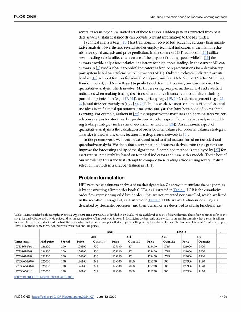
Table 1. Limit order book example: Wartsila Oyj on 01 June 2010. LOB is divided in 10 levels, where each level consists of four columns. These four columns refer to the

ask price and volume and the bid price and volume, respectively. The best level is Level 1. It contains the best Ask price which is the minimum price that a seller is willing

to accept for a share of stock and the best Bid price which is the maximum price that a buyer is willing to pay for a share of stock. Next to Level 1 is Level 2 and so on, up to

Level 10 with the same formation but with worst Ask and Bid prices.

Level 1 Level 2 . . .

Ask Bid Ask Bid

Timestamp Mid-price Spread Price Quantity Price Quantity Price Quantity Price Quantity

1275386347944 126200 200 126300 300 126100 17 126400 4765 126000 2800 . . .

1275386347981 126200 200 126300 300 126100 17 126400 4765 126000 2800 . . .

1275386347981 126200 200 126300 300 126100 17 126400 4765 126000 2800 . . .

1275386348070 126050 100 126100 291 126000 2800 126200 300 125900 1120 . . .

1275386348070 126050 100 126100 291 126000 2800 126200 300 125900 1120 . . .

1275386348101 126050 100 126100 291 126000 2800 126200 300 125900 1120 . . .

https://doi.org/10.1371/journal.pone.0234107.t001





[2]). The functions are formulated for a specific limit order (i.e. an order with specific charac-

teristics in terms of price and volume at a specific time t), as t), as: order = (t, Pricet, Volumet)that becomes active at time t holds that: order 2 LðtÞ; order =2 limorder0"orderx

Lðorder0Þ. Depend-

ing on how the LOB is constructed, we treat the new information according to event arrivals.

The objective of our work is to predict the direction (i.e. up, down, or stationary) of the mid-

price (i.e. (pa + pb)/2, where pa is the ask price and pb is the bid price at the first level of LOB).

The goal is to utilize informative features based on the order flow (i.e. message list or message

book [MB]) and LOB, which will help the ML trader improve the accuracy of mid-price move-

ment prediction.

Feature pool

Limit Order Book (LOB) and Message Book (MB) are the main sources from which features

are extracted. We provide a comprehensive list of features explored in the literature for tech-

nical and quantitative trading in Table 3. The description of the hand-crafted features, except

the newly introduced feature, named Adaptive Logistic Regression feature, is provided in the

Appendix where the description of the newly introduced feature, named Adaptive Logistic

Regression feature, follows. The motivation for choosing the suggested list of features is

based on an examination of all the basic and advanced features from technical analysis and

comparisons with advanced statistical models, such as adaptive logistic regression for online

learning. The present work has identified a gap in the existing literature concerning the per-

formance of technical indicators and comparisons with quantitative models. This work sets

the ground for future research since it provides insight into the features that are likely to

achieve a high rank on the ordering list in terms of predictability power. To this end, we

divide our feature sets into three main groups. The first group of features is extracted accord-

ing to [28] and [29]. This group of features aims to capture the dynamics of the LOB. This is

possible if we consider the actual raw LOB data and relative intensities of different look-back

periods of the trade types (i.e. order placement, execution, and cancellation). The second

group of features is based on technical analysis. The suggested list describes many of the

existing technical indicators (basic and advanced). Technical indicators might help traders

spot hidden trends and patterns in their time series. The third group of features is derived

according to quantitative analysis, which is mainly based on statistical models; it can provide

statistics that are hidden in the data. This can be verified by the ranking process, where the

proposed advanced online feature (i.e. adaptive logistic regression) is ranked first in most of

the feature selection metrics (i.e. four out of five feature lists). The suggested features are fully

described in the Appendix; whereas, the proposed adaptive logistic regression feature is

described next.

Table 2. Message list example: Wartsila Oyj on 01 June 2010. This a typical message book which contains the raw trading information. Every message book row contains

information regarding the trade arrival time, trade id, stock price, stock volume, event type and side of the trade.

Timestamp Id Price Volume Event Side

1275377039033 1372349 341100 300 Submission Bid

1275377039033 1372349 341100 300 Cancellation Bid

1275377039037 1370659 343700 100 Submission Ask

1275377039037 1370659 343700 100 Cancellation Ask

1275377039037 1372352 341700 150 Submission Bid

1275377039037 1372352 341700 150 Cancellation Bid






Table 3. Feature list for the three groups.

Feature Sets Description

First group:

Basic n levels of LOB Data

Time-Insensitive Spread & Mid-Price

Price Differences

Price & Volume Means

Accumulated Differences

Time-Sensitive Price & Volume Derivation

Average Intensity per Type

Relative Intensity Comparison

Limit Activity Acceleration

Second group:

Technical Analysis

Accumulation Distribution Line Awesome Oscillator

Accelerator Oscillator Average Directional Index

Average Directional Movement Index Rating Displaced Moving Average based on Williams Alligator

Indicator

Absolute Price Oscillator Aroon Indicator

Aroon Oscillator Average True Range

Bollinger Bands Ichimoku Clouds

Chande Momentum Oscillator Chaikin Oscillator

Chandelier Exit Center of Gravity Oscillator

Donchian Channels Double Exponential Moving Average

Detrended Price Oscillator Heikin-Ashi

Highest High and Lowest Low Hull MA

Internal Bar Strength Keltner Channels

Moving Average Convergence/Divergence

Oscillator

Median Price

Momentum Variable Moving Average

Normalized Average True Range Percentage Price Oscillator

Rate of Change Relative Strength Index

Parabolic Stop and Reverse Standard Deviation

Stochastic Relative Strength Index T3-Triple Exponential Moving Average

Triple Exponential Moving Average Triangular Moving Average

Triple Exponential Average True Strength Index

Ultimate Oscillator Weighted Close

Williams %R Zero-Lag Exponential Moving Average

Fractals Linear Regression Line

Digital Filtering: Rational Transfer Function Digital Filtering: Savitzky-Golay Filter

Digital Filtering: Zero-Phase Filter Remove Offset and Detrend

Beta-like Calculation

Third group:

Quantitative Analysis

Autocorrelation

Partial Correlation

Cointegration based on Engle-Granger test

Order Book Imbalance

Adaptive Logistic Regression






Proposed adaptive logistic regression feature

We introduce a novel logistic regression model that we use as a feature in our experimental

protocol. The motivation for this model is the work done in [4] where the focal point is the

local behavior of LOB levels. We extend this idea by doing online learning with an adaptive

learning rate. The new feature operates under an online learning mechanism by taking into

consideration the latest trading event of the 10-event message book block which means that

the forecasting of the next mid-price move is updated according to the latest information flow.

More specifically, we use the Hessian matrix as our adaptive rate. We also report the ratio of

the logistic coefficients based on the relationship of the LOB levels close to the best LOB level

and the ones which are deeper in the LOB. Since 0� hθ(V)�1 and V are the stock volumes for

the first best six levels of the LOB, we formulate the model as follows:

hyðVÞ ¼1

1þ e� yTVð1Þ

be the logistic function (i.e. Hypothesis function) and yTV ¼ y0 þ

Xn

j¼1

yjVj. Parameter estima-

tion is considered by calculating the parameter’s likelihood:

LðyÞ ¼Ym

i¼1

ðhyðVðiÞÞÞ

yðiÞð1 � hyðV

ðiÞÞÞ1� yðiÞ

ð2Þ

form training samples and the cost function, based on this probabilistic approach, is as fol-

lows:

JðyÞ ¼1

m

Xm

i¼1

� yðiÞlogðhyðVðiÞÞÞ � ð1 � yðiÞÞlogð1 � hyðV

ðiÞÞÞ� �

: ð3Þ

The next step is the process of choosing θs for optimizing (i.e. minimizing) J(θ). To do so,

we will use Newton’s update method:

yðsþ1Þ¼ y

ðsÞ� H� 1ryJ; ð4Þ

where the gradient is:

ryJ ¼1

m

Xm

1

ðhyðVðiÞÞ � yðiÞÞVðiÞ ð5Þ

and the Hessian matrix is:

H ¼1

m

Xm

i¼1

hyðVðiÞÞ 1 � hyðV

ðiÞÞ� �

VðiÞðV ðiÞÞT� �

ð6Þ

with VðiÞðVðiÞÞT 2 Rðnþ1Þ�ðnþ1Þand y(i) are the labels which are calculated as the differences of

the best level’s ask (and bid) prices. The suggested labels describe a binary classification prob-

lem since we consider two states, one for change in the best ask price and another one for no

change in the best ask price.

We perform the above calculation in an online manner. The online process considers the

9th element of every 10 MB block multiplied by the θ coefficient first-order tensor to obtain the

probabilistic behavior (we filter the obtained first-order tensor through the hypothesis func-

tion) of the 10th event of the 10 MB block. The output is the feature representation expressed

as a scalar (i.e. probability) of the bid and ask price separately.




Wrapper method of feature selection

Feature selection is an area that focuses on applications with multidimensional datasets. A ML

trader performs feature selection for three primary reasons: to reduce computational complex-

ity, to improve performance, and to gain a better understanding of the underlying process.

Feature selection, as a pre-processing method, can enhance classification power by adding fea-

tures that contain information relevant to the task at hand. There are two metaheuristic feature

selection methods: the wrapper method and the filter (i.e. transformation) -based method. We

choose to perform classification based on the wrapper method since it considers the relation-

ship among the features while filter methods do not.

Our wrapper approach consists of five different feature subset selection criteria based on

two linear and one non-linear methods for evaluation with a general description in Algorithm

1 where: lopt is the optimal feature list per criterion, Feature_Select is the name of the function

algorithm, X is the input feature set, labels represent the movements of mid-price, l is the cur-

rent feature list up to D feature dimensions, N is the sample size, curr_X is the current input

data up to the current number i of the features together with the optimal ones up to i, and

best_d is a vector that saves the best feature out of the entire list of features. More specifically,

we convert entropy, LMS, and LDA as feature selection criteria. For the last two cases (i.e.,

LMS and LDA) we provide two different selection criteria as follows: i) for LMS the first metric

follows the L2-norm and the second metric is a statistical bias measure, and ii) for LDA the

first metric is based on the ratio of the within-class scatter matrix while the second metric is

derived according to the between-class scatter matrix. For classification evaluation we utilize

LMS, LDA and a radial basis function network (i.e., [30]) as these were used in [29] and [31].

Our choice to apply these linear and non-linear classifiers is informed by the amount of data

in our dataset (details will be provided in the following section). We measure classification per-

formance according to accuracy, precision, recall, and F1 scores for every possible combina-

tion of the hand-crafted features by using LMS, LDA, and RBF ANN. These perfromance

measures are defined as follows:

Accuracy ¼TPþ TN

TP þ TN þ FP þ FNð7Þ

Precision ¼TP

TP þ FPð8Þ

Recall ¼TP

TP þ FNð9Þ

F1 ¼ 2�Precision� RecallPrecisionþ Recall

ð10Þ

where TP and TF represents the true positives and true negatives, respectively, of the mid-

price prediction label compared with the ground truth, where FP and FN represents the false

positives and false negatives, respectively.

Algorithm 1 Wrapper-Based Feature Selection1: procedure lopt = Feature_SelectX, labels, criterion2: l = [1: D]3: lopt = []4: Xopt = [], [D, N] = size(X)5: for d = 1: D do6: crit_list = []




7: for i = 1: D − d + 1 do8: curr_X = [Xopt;X(i;:)]9: crit_list[i] = crit(curr_X)10: end for11: [best_d, best_crit] = opt(crit_list)12: lopt[d] = best_d13: l[best_d] = []14: Xopt = [Xopt;X(best_d;:)]15: X(best_d,:) = []16: end for17: end procedure

Feature sorting

We convert sample entropy, LMS, and LDA (for the latter two methods we use two different

criteria for feature evaluation) into feature selection methods. A visual representation of the

feature sorting method can be seen in Fig 2. It can be briefly described as follows: the process

of feature sorting and classification is based on the wrapper method. From left to right: 1) Raw

data is converted to LOB data via superclustering, 2) the feature extraction process follows

(i.e., three feature sets are extracted), 3) then every feature set is normalized based on z-score

in a rolling window, 4) Wrapper method: there are two main blocks in this process—the first

block refers to sorting (i.e., five different sorting criteria based on entropy, LMS1, LMS2,

LDA1, and LDA2) of the feature sets independently (i.e., LOB features, technical indicators,

and quantitative indicators are sorted separately) and all together (i.e., the three feature sets are

merged and sorted all together) and the second block refers to the incremental classification

(i.e., we increase the dimension of each sorting list during classification by one feature in each

Fig 2. Wrapper method: Starting from the top left of the flow chart, we use MB and LOB data for feature extraction (i.e., LOB,

technical and quantitative features). The next step is the z-score normalization of the suggested feature representations which are

used as inputs to the wrapper protocol. The wrapper protocol is the main block of our experimental analysis. This main block is

divided into two secondary blocks (i.e., yellow-colored blocks). The top yellow block acts as an incremental sorting method since it

uses five different methods (i.e., entropy, LMS1, LMS2, LDA1, and LDA2) for feature evaluation. When the five sorted feature lists

are ready then each sorted feature goes through a classifier (i.e., three different classifiers in our case based on RBFN, LDA, and

LMS). This last part of the wrapper topology performs the classification task of the mid-price movement prediction.






loop and average the final F1 scores per sorting list) based on three classifiers (i.e., LMS, LDA,

and RBFN).

Feature sorting with entropy. We employ entropy [32], which is a measure of signal

complexity where the signal is the time series of the multidimensional two-mode tensor with

dimensions Rp�n, and where p is the number of features and n is the number of samples, as a

measure of feature relevance. We calculate the bits of each feature in the feature set iteratively

and report the order. We measure the entropy as follows:

HðXÞ ¼ �Xp

i¼1

pðxiÞ log pðxiÞ; ð11Þ

where p(xi) is the probability of the frequency per feature for the given data samples.

Feature sorting with least-mean-squares. We perform feature selection based on the

least-mean square classification rate (LMS1) and L2-norm (LMS2). LMS is a fitting method

that aims to produce an approximation that minimizes the sum of squared differences between

given data and predicted values. We use this approach to evaluate the relevance of our hand-

crafted features. A hand-crafted feature evaluation is performed sequentially via LMS. More

specifically, each of the features is evaluated based on the classification rate, the L2-norm of

the predicted labels, and the ground truth. The evaluation process is performed as follows:

HW ¼ T; ð12Þ

where H 2 Rpi�n is the input data with feature dimension pi which is calculated incrementally

for the number of training samples n, W 2 Rpi�#cl are the weighted coefficients for the number

of features pi of the number() of classes (i.e. up, down, and stationary labelling), and T 2 R#cl�n

represents the target labels of the training set. The weight coefficient matrix W is estimated via

the following formula:

W ¼ HyT; ð13Þ

where H† is the Moore-Penrose pseudoinverse matrix.

Feature sorting with linear discriminant analysis. Linear discriminant analysis (LDA)

can be used for classification and dimensionality reduction. However, instead of performing

these two tasks, we convert LDA into a feature selection algorithm. We measure feature selec-

tion performance based on two metrics. One is the classification rate (LDA1) and the other is

based on the error term (LDA2), which we define as the ratio of the within-class scatter matrix

and the between-class scatter matrix. The main objective of LDA is finding the projection

matrix W 2 Rm�#cl� 1, wherem is the sample dimension, and cl is the number of classes, such

that Y =WT Xmaximizes the class separation. For the given sample set X = X1[X2[. . .[X#cl,

where Xk ¼ fxk1; :::; xk‘kgk¼1;:::;#cl

is the class-specific data subsample, we need to find W that

maximizes the Fisher’s ratio:

JðWÞ ¼traceðWTSBWÞtraceðWTSWWÞ

; ð14Þ

where

SB ¼X#cl

i¼1

Niðmi � mÞðmi � mÞT

ð15Þ




and

SW ¼XC

i¼1

Xd

x2Xi

ðx � miÞðx � miÞT

ð16Þ

are the between-class and within-class scatter matrices, respectively, with mi ¼1

‘k

X

k2#cl

Xk and

m ¼ 1

m

X

k2#cl

‘kXk. In a similar fashion, we compute the projected samples y with ~mi ¼1

‘k

X

k2#cl

Yk

and ~m ¼ 1

m

X

k2#cl

‘kYk, while the scatter matrices (i.e. within and between scatter matrices, respec-

tively) are

fSW ¼X#cl

i¼1

X

k2#cl

ðy � ~miÞðy � ~miÞT

ð17Þ

and

eSB ¼X#cl

i¼1

‘kð ~mi � ~mÞð ~mi � ~mÞT: ð18Þ

The above calculations constitute the basis for the two metrics that we use to evaluate 285

the hand-crafted features incrementally. The two evaluation metrics are based on the 286 clas-

sification rate and the ratio of the within-class and between-class scatter matrices of the pro-

jected space Y.

Classification for feature selection

We perfrom classification evaluation based on three classifiers: LMS, LDA, and RBFN. The

basic concept of the first two methods was discussed above while RBFN classifier is described

in the following section.

RBFN classifier. We utilize a single-layer feedforward neural network (SLFN) as this sug-

gested by [33]. A detailed description and the implementation of the method can be found in

[29]. In order to train this model fast, we follow the procedures outlined in [34], and [35]. We

use K-means clustering for K prototype vectors identification, which then are used as the net-

work’s hidden layer weights. After determining the the network’s hidden layer weights

V 2 RD�K , the input data xi, i = 1, . . ., N are mapped to vectors hi 2 RK

in the feature space

determined by the network’s hidden layer outputs RK . Then a radial basis function is used, i.e.

hi = ϕRBF(xi), calculated in an element-wise manner, as follows:

hik ¼ expk xi � vk k2

2

2s2

� �

; k ¼ 1; � � � ;K; ð19Þ

where σ is a hyper-parameter denoting the spread of the RBF neuron and vk corresponds to

the k-th column of V.

The network’s output weights W 2 RK�C are determined by solving the following equation:

W� ¼ argminW

kWTH � T k2

F þl kW k2

F; ð20Þ

where H = [h1, . . ., hN] is a matrix formed by the network’s hidden layer outputs for the train-

ing data and T is a matrix formed by the network’s target vectors ti, i = 1, . . ., N. The network’s




output weights are given by:

W ¼ ðHHT þ lIÞ� 1HTT: ð21Þ

Then a new (test) sample x 2 RD is mapped to its corresponding representations in spaces

RK and RC, i.e. h = ϕRBF(x) and o = WT h, respectively. Finally, the classification task is based

on the maximal network output, i.e.:

lx ¼ argmaxk

ok: ð22Þ

Experimental results

In this section, we provide details regarding the conducted experiments. The goal of the exper-

iments is to predict the mid-price state (i.e. up, down, and stationary) for ITCH feed data in

millisecond resolution (ITCH is a type of direct data-feed protocol and the acronym according

to Nasdaq carry no semantic meaning). Additional information regarding the dataset can be

found in [29]). For the experimental protocol, we followed the setup in [29], which is based on

the anchored cross-validation format. According to this format, we use the first day as training

and the second day as testing for the first fold, whereas the second fold consists of the previous

training and testing periods as a training set, and the next day is always used as the test set.

Each of the training and testing sets contains the hand-crafted feature representations for all

the five stocks from the FI-2010 dataset. Hence, we obtain a mode-three tensor of dimensions

273 × 458, 125. The first dimension is the number of features, whereas the second one is the

number of sample events. At this point, we must specify that the process of hand-crafted fea-

ture extraction is conducted in the full length of the given information based on MB with

4,581,250 events. The motivation for taking separate blocks of messages of ten events is the

time-invariant nature of the data. To keep the ML trader fully informed regarding MB blocks,

we use features that convey this information by calculating, among others, price and volume

averages, regression coefficients, risk factors, and online learning feedback indicators.

The results we present here are the mid-price predictions for the next 10th, 20th, and 30th

events (i.e. translated into MB events) or else one, two, and three next events after the current

state translated into a feature representation setup. The prediction performance of these events

is measured by the accuracy, precision, recall and F1 score, whereas F1 score is further empha-

sized, as it can only be affected in one direction by skewed distributions for unbalanced classes,

as observed in our data. Performance metrics are calculated against mid-price labelling calcu-

lation of ground truth extraction. More specifically, we extract labels based on the percentage

change of the smoothed mid-price with a span window of 9, for our supervised learning meth-

ods, computed as follows: L1 ¼MPnext � MPcurr

MPcurr, whereMPcurr is the current mid-price, and

MPnext is the next mid-price. The percentage change identification is thresholded by an empir-

ically fixed value γ = 0.002 rolling z-score normalization is performed on the dataset to avoid

look-ahead bias (look ahead bias refers to the process that future information is injected to the

training set). The rolling window z-score normalization is based on the anchored cross-valida-

tion setup which means that the normalization of the training set is unaffected by any future

information.

We report our results in Tables 4–8 for each possible combination of feature set, sorting

and classification method used. RBFN classifier operates under the extreme learning machine

model with a slight modification in the initialization process of weights calculation based on

the K-means algorithm. The full description of this method can be found in [29]. We provide




results based on the whole feature pool (see Table 4), the first feature pool according to [28]

and [29] (see Table 5), based only on technical indicators (see Table 6) and the quantitative

indicators (see Table 7). More specifically, for the first feature pool, we have 136 features, while

for the second pool we have 82 features, and for the last pool we have 55 features; in total, we

have 273 features.

The number of top features that used in the above methods is different in each case and can

be monitored in Figs 3 and 4. We should point out that we tested all the possible combinations

for the five sorting methods and the three classifiers (i.e., 15 different cases) but we report only

results that exhibit some variations. For instance, in Tables 5–7 we report results for entropy as

Table 4. Results based on the total feature pool—273 features. Bold text highlights the best F1 performance per predicted horizon T. LMS classifier achieved the best F1

performance for every predicted horizon.

Sorting Classifier T Accuracy Precision Recall F1

Entropy LMS 10 0.529 ± 0.059 0.447 ± 0.007 0.477 ± 0.013 0.440 ± 0.018

LMS1 LMS 10 0.540 ± 0.059 0.437 ± 0.007 0.456 ± 0.013 0.430 ± 0.018

LMS2 LMS 10 0.538 ± 0.052 0.447 ± 0.005 0.478 ± 0.013 0.444 ± 0.011

LDA1 LDA 10 0.616 ± 0.048 0.408 ± 0.019 0.398 ± 0.011 0.397 ± 0.015

LDA2 LDA 10 0.543 ± 0.057 0.430 ± 0.010 0.455 ± 0.017 0.429 ± 0.018

LDA1 LMS 10 0.604 ± 0.068 0.468 ± 0.035 0.431 ± 0.042 0.408 ± 0.035

LDA2 LMS 10 0.522 ± 0.026 0.441 ± 0.020 0.473 ± 0.007 0.435 ± 0.007

Entropy RBFN 10 0.474 ± 0.046 0.420 ± 0.031 0.445 ± 0.039 0.400 ± 0.039

LMS1 RBFN 10 0.600 ± 0.045 0.436 ± 0.019 0.425 ± 0.021 0.417 ± 0.019

LMS2 RBFN 10 0.537 ± 0.016 0.442 ± 0.011 0.470 ± 0.016 0.439 ± 0.012

LDA1 RBFN 10 0.585 ± 0.061 0.443 ± 0.018 0.438 ± 0.037 0.419 ± 0.026

LDA2 RBFN 10 0.528 ± 0.029 0.438 ± 0.020 0.467 ± 0.010 0.434 ± 0.017

Entropy LMS 20 0.503 ± 0.049 0.469 ± 0.008 0.482 ± 0.014 0.462 ± 0.017

LMS1 LMS 20 0.503 ± 0.049 0.470 ± 0.008 0.482 ± 0.014 0.462 ± 0.017

LMS2 LMS 20 0.503 ± 0.049 0.469 ± 0.008 0.481 ± 0.014 0.462 ± 0.018

LDA1 LDA 20 0.478 ± 0.060 0.400 ± 0.038 0.404 ± 0.041 0.393 ± 0.018

LDA2 LDA 20 0.505 ± 0.046 0.452 ± 0.009 0.461 ± 0.012 0.450 ± 0.012

LDA1 LMS 20 0.530 ± 0.032 0.457 ± 0.024 0.426 ± 0.048 0.401 ± 0.048

LDA2 LMS 20 0.499 ± 0.019 0.462 ± 0.019 0.476 ± 0.007 0.457 ± 0.015

Entropy RBFN 20 0.464 ± 0.038 0.436 ± 0.033 0.448 ± 0.035 0.425 ± 0.036

LMS1 RBFN 20 0.519 ± 0.023 0.430 ± 0.016 0.417 ± 0.022 0.412 ± 0.027

LMS2 RBFN 20 0.508 ± 0.010 0.456 ± 0.015 0.466 ± 0.018 0.454 ± 0.017

LDA1 RBFN 20 0.523 ± 0.025 0.441 ± 0.024 0.429 ± 0.041 0.416 ± 0.046

LDA2 RBFN 20 0.502 ± 0.018 0.454 ± 0.019 0.465 ± 0.009 0.452 ± 0.015

Entropy LMS 30 0.503 ± 0.042 0.475 ± 0.013 0.484 ± 0.014 0.470 ± 0.019

LMS1 LMS 30 0.503 ± 0.042 0.475 ± 0.013 0.484 ± 0.014 0.470 ± 0.019

LMS2 LMS 30 0.503 ± 0.043 0.474 ± 0.012 0.482 ± 0.014 0.461 ± 0.019

LDA1 LDA 30 0.464 ± 0.048 0.414 ± 0.025 0.420 ± 0.027 0.403 ± 0.018

LDA2 LDA 30 0.500 ± 0.043 0.457 ± 0.012 0.464 ± 0.013 0.455 ± 0.014

LDA1 LMS 30 0.489 ± 0.018 0.451 ± 0.030 0.429 ± 0.051 0.405 ± 0.072

LDA2 LMS 30 0.496 ± 0.016 0.476 ± 0.018 0.479 ± 0.009 0.472 ± 0.015

Entropy RBFN 30 0.464 ± 0.035 0.446 ± 0.035 0.449 ± 0.034 0.440 ± 0.037

LMS1 RBFN 30 0.471 ± 0.018 0.425 ± 0.018 0.414 ± 0.020 0.409 ± 0.026

LMS2 RBFN 30 0.494 ± 0.014 0.464 ± 0.021 0.466 ± 0.021 0.461 ± 0.024

LDA1 RBFN 30 0.481 ± 0.022 0.438 ± 0.034 0.428 ± 0.045 0.415 ± 0.057

LDA2 RBFN 30 0.493 ± 0.017 0.465 ± 0.018 0.467 ± 0.010 0.463 ± 0.016






sorting method and LMS together with RBFN as classifiers but not with LDA (as a classifier)

since the last method reports similar results. We focus on F1 score and particularly on

F1-macro (i.e., F1-macro = 1

C

Pk2CF1k, with C as the number of classes for the 9-fold experi-

mental protocol) results, based on the total feature pool, for the five sorting lists classified per

LMS, LDA, and RBFN for the next T = 10th, 20th, and 30th events, respectively, as the predicted

horizon. Again, as the number of top features used in the above methods is different in each

case (as seen in Fig 3), it can be briefly described as follows: Bar plots with variance presents

the average (i.e. average F1 performance for the 9-fold protocol for all the features) F1 score of

the 12 different models for the cases of 5, 50, 100, 200, and 273 number of top features. The

order of the models from the left to the right column is:

Table 5. Results based on the hand-crafted features based on LOB features—136 features. Bold text highlights the best F1 performance per predicted horizon T. LMS

classifier achieved the best F1 performance for every predicted horizon.


Entropy LMS 10 0.420 ± 0.025 0.379 ± 0.011 0.397 ± 0.011 0.355 ± 0.013

LMS1 LMS 10 0.574 ± 0.055 0.402 ± 0.013 0.396 ± 0.018 0.384 ± 0.020

LMS2 LMS 10 0.519 ± 0.015 0.400 ± 0.009 0.413 ± 0.009 0.396 ± 0.010

LDA1 LDA 10 0.561 ± 0.090 0.389 ± 0.018 0.382 ± 0.016 0.363 ± 0.030

LDA2 LDA 10 0.507 ± 0.041 0.373 ± 0.014 0.384 ± 0.017 0.362 ± 0.019

Entropy LMS 20 0.386 ± 0.018 0.386 ± 0.015 0.397 ± 0.015 0.363 ± 0.016

LMS1 LMS 20 0.527 ± 0.027 0.411 ± 0.013 0.389 ± 0.015 0.375 ± 0.029

LMS2 LMS 20 0.462 ± 0.013 0.405 ± 0.013 0.410 ± 0.009 0.400 ± 0.012

LDA1 LDA 20 0.529 ± 0.031 0.406 ± 0.017 0.381 ± 0.011 0.360 ± 0.024

LDA2 LDA 20 0.461 ± 0.036 0.378 ± 0.016 0.380 ± 0.016 0.368 ± 0.021

Entropy LMS 30 0.391 ± 0.016 0.395 ± 0.018 0.401 ± 0.015 0.380 ± 0.017

LMS1 LMS 30 0.459 ± 0.025 0.405 ± 0.017 0.388 ± 0.020 0.366 ± 0.040

LMS2 LMS 30 0.432 ± 0.009 0.407 ± 0.015 0.409 ± 0.013 0.401 ± 0.016

LDA1 LDA 30 0.447 ± 0.041 0.391 ± 0.018 0.377 ± 0.017 0.352 ± 0.037

LDA2 LDA 30 0.418 ± 0.028 0.373 ± 0.016 0.375 ± 0.015 0.361 ± 0.018


Table 6. Results based only on technical indicators—82 features. Bold text highlights the best F1 performance per predicted horizon T. LMS classifier achieved the best

F1 performance for every predicted horizon.


Entropy LMS 10 0.456 ± 0.038 0.372 ± 0.021 0.380 ± 0.014 0.353 ± 0.020

LMS1 LMS 10 0.497 ± 0.066 0.371 ± 0.017 0.377 ± 0.021 0.354 ± 0.024

LMS2 LMS 10 0.460 ± 0.016 0.383 ± 0.012 0.394 ± 0.009 0.365 ± 0.010

LDA1 LDA 10 0.517 ± 0.064 0.367 ± 0.015 0.371 ± 0.020 0.344 ± 0.026

LDA2 LDA 10 0.475 ± 0.023 0.371 ± 0.010 0.382 ± 0.009 0.351 ± 0.015

Entropy LMS 20 0.430 ± 0.029 0.384 ± 0.025 0.387 ± 0.017 0.371 ± 0.023

LMS1 LMS 20 0.480 ± 0.033 0.384 ± 0.023 0.381 ± 0.021 0.364 ± 0.037

LMS2 LMS 20 0.452 ± 0.011 0.400 ± 0.018 0.402 ± 0.011 0.391 ± 0.015

LDA1 LDA 20 0.483 ± 0.034 0.379 ± 0.022 0.377 ± 0.020 0.355 ± 0.038

LDA2 LDA 20 0.453 ± 0.014 0.382 ± 0.015 0.387 ± 0.009 0.369 ± 0.016

Entropy LMS 30 0.423 ± 0.030 0.394 ± 0.028 0.394 ± 0.020 0.385 ± 0.027

LMS1 LMS 30 0.450 ± 0.018 0.395 ± 0.028 0.393 ± 0.027 0.379 ± 0.050

LMS2 LMS 30 0.446 ± 0.013 0.409 ± 0.020 0.408 ± 0.013 0.403 ± 0.019

LDA1 LDA 30 0.430 ± 0.041 0.384 ± 0.027 0.382 ± 0.027 0.353 ± 0.053

LDA2 LDA 30 0.433 ± 0.021 0.397 ± 0.017 0.396 ± 0.016 0.386 ± 0.026







1. feature list sorted based on entropy and classified based on LMS,

2. feature list sorted based on LMS1 and classified based on LMS,

3. feature list sorted based on LMS2 and classified based on LMS,

4. feature list sorted based on LDA1 and classified based on LDA,

5. feature list sorted based on LDA2 and classified based on LDA,

6. feature list sorted based on LDA1 and classified based on LMS,



9. feature list sorted based on entropy and classified based on RBFN,

Table 7. Results based on quantitative features—55 features. Bold text highlights the best F1 performance per predicted horizon T. LMS classifier achieved the best F1

performance for every predicted horizon.


Entropy LMS 10 0.393 ± 0.109 0.399 ± 0.047 0.419 ± 0.047 0.340 ± 0.064

LMS1 LMS 10 0.665 ± 0.033 0.468 ± 0.043 0.388 ± 0.016 0.366 ± 0.016

LMS2 LMS 10 0.571 ± 0.071 0.470 ± 0.053 0.418 ± 0.032 0.384 ± 0.020

LDA1 LDA 10 0.611 ± 0.088 0.422 ± 0.039 0.390 ± 0.020 0.370 ± 0.024

LDA2 LDA 10 0.380 ± 0.101 0.401 ± 0.024 0.428 ± 0.027 0.339 ± 0.063

Entropy LMS 20 0.400 ± 0.074 0.408 ± 0.048 0.422 ± 0.048 0.372 ± 0.061

LMS1 LMS 20 0.553 ± 0.029 0.429 ± 0.037 0.373 ± 0.016 0.335 ± 0.025

LMS2 LMS 20 0.483 ± 0.017 0.447 ± 0.022 0.457 ± 0.025 0.435 ± 0.029

LDA1 LDA 20 0.513 ± 0.072 0.402 ± 0.032 0.379 ± 0.026 0.347 ± 0.040

LDA2 LDA 20 0.424 ± 0.073 0.431 ± 0.026 0.444 ± 0.023 0.340 ± 0.053

Entropy LMS 30 0.410 ± 0.062 0.416 ± 0.051 0.423 ± 0.048 0.391 ± 0.060

LMS1 LMS 30 0.478 ± 0.022 0.407 ± 0.038 0.370 ± 0.019 0.320 ± 0.036

LMS2 LMS 30 0.481 ± 0.012 0.457 ± 0.026 0.460 ± 0.024 0.449 ± 0.034

LDA1 LDA 30 0.464 ± 0.037 0.394 ± 0.030 0.378 ± 0.027 0.338 ± 0.049

LDA2 LDA 30 0.425 ± 0.063 0.437 ± 0.029 0.443 ± 0.022 0.406 ± 0.055


Table 8. F1 based on different numbers of best features for the five criteria. Bold text highlights the best F1 performance for the predicted horizon T = 10. LMS classifier

achieved the best F1 performance for every predicted horizon.

Sorting Classifier 5 50 100 200 273

Entropy LMS 0.319 ± 0.008 0.363 ± 0.027 0.414 ± 0.020 0.425 ± 0.025 0.440 ± 0.018

LMS1 LMS 0.377 ± 0.008 0.374 ± 0.036 0.393 ± 0.047 0.419 ± 0.036 0.440 ± 0.018

LMS2 LMS 0.402 ± 0.015 0.443 ± 0.014 0.441 ± 0.018 0.440 ± 0.018 0.440 ± 0.018

LDA1 LMS 0.373 ± 0.013 0.380 ± 0.017 0.395 ± 0.016 0.315 ± 0.018 0.289 ± 0.025

LDA2 LMS 0.412 ± 0.011 0.420 ± 0.017 0.420 ± 0.019 0.289 ± 0.013 0.309 ± 0.027

LDA1 LMS 0.370 ± 0.011 0.372 ± 0.032 0.387 ± 0.041 0.440 ± 0.017 0.440 ± 0.018

LDA2 LMS 0.421 ± 0.010 0.435 ± 0.011 0.435 ± 0.014 0.440 ± 0.017 0.441 ± 0.018

Entropy RBFN 0.316 ± 0.010 0.363 ± 0.020 0.413 ± 0.016 0.430 ± 0.016 0.441 ± 0.016

LMS1 RBFN 0.387 ± 0.018 0.402 ± 0.022 0.421 ± 0.017 0.429 ± 0.017 0.441 ± 0.016

LMS2 RBFN 0.403 ± 0.015 0.444 ± 0.012 0.439 ± 0.013 0.439 ± 0.019 0.442 ± 0.016

LDA1 RBFN 0.371 ± 0.011 0.387 ± 0.021 0.411 ± 0.013 0.440 ± 0.016 0.441 ± 0.016

LDA2 RBFN 0.416 ± 0.011 0.434 ± 0.015 0.436 ± 0.015 0.436 ± 0.016 0.442 ± 0.016







Fig 3. Bar plots for the F1 scores of the 12 different experimental models. This bar plot shows that an extensive feature selection

mechanism is vital for a trader to identify the top candidates/indicators that can boost the classification performance. Several

classifiers combined with a limited number of sorted hand-crafted features reached their top performance while some other

classifiers reported lower F1 performance with more (sorted) features.


Fig 4. F1 performance per number of best features sequence for 10 events. This graph displays the same information as the bar

plot above but also provides every model’s performance for every possible number of the sorted hand-crafted features.







10. feature list sorted based on LMS2 and classified based on RBFN,

11. feature list sorted based on LDA1 and classified based on RBFN, and

12. feature list sorted based on LDA2 and classified based on RBFN.

There is a dual interpretation of the suggested feature lists and wrapper method results.

Regarding the feature lists, we have five different feature sorting methods starting from

entropy, to LMS1 and LMS2 and continue to LDA1 and LDA2. More specifically, results based

on the entropy sorting method reveal that the top 20 features almost entirely come from tech-

nical indicators (i.e. only 1 out of 20 comes from the first basic group), while the first 100 top

ranked features include 36 quant features, 48 technical features, and 16 features from the first

basic group.

For the LMS case, we present two sorting lists where we use two different criteria for the

final feature selection. In the LMS1 case, the top 20 features are derived mainly from quantita-

tive analysis (11 out of 20), 7 features come from the first basic group, and only 2 from the

technical group of features. The top (best) feature is the proposed advanced feature based on

the logistic regression model for online learning. For the same method, the first 100 best fea-

tures include 25 quant features, 18 technical features, and the remaining 57 features come

from the first basic group. In the LMS2 case, the first top 20 features include 7 quant, 9 techni-

cal, and only 4 features from the first basic group. LMS2 also selects the advanced feature

based on the logistic regression model for online learning as its first top feature.

The last method that we use as the basis for the feature selection process is based on LDA.

Similarly, we use two different criteria as a measure for the selection process. In LDA1, the

first top 20 features include 10 quant, 3 technical, and 7 from the first basic group. The first top

100 features include 19 quant, 20 technical, and the remaining 61 features come from the first

basic group. Again, the first top feature is the proposed advanced feature based on the logistic

regression model for online learning. The last feature selection model, LDA2, selects 6 features

from the quant pool, 6 from the technical pool, and 8 from the first basic group. LDA2 selects

as the first top 100 features, 24 quant, 27 technical, and 49 features from the first basic group.

The top 10 are listed for each of the 5 sorting methods in Table 9.

The second interpretation of our findings is the performance of the 12 different classifiers

(based on LMS, LDA, and RBFN) used to measure, in terms of F1 score, the predictability of

the mid-price movement. Fig 3 provides an overview of the F1 score performance in terms of

best feature numbers and classifiers. We can divide these twelve models (pairs based on the

sorting and classification method) into three groups according to their response in terms of

information flow. The first group, where LMS2-LMS, LDA2-LMS, LMS2-RBFN, and

LDA2-RBFN belong, reach their plateau very early in the incremental process of adding less

informative features. These models were able to reach (close to) their maximum F1 score per-

formance with approximately 5 top features, which means that the dimensionality of the input

matrix to the classification model is quite small. The second group of models, Entropy-LMS,

LMS1-LMS, LDA1-LMS, Entropy-RBFN, LMS1-RBFN, and LDA1-RBFN, had a slower reac-

tion in the process of reaching their top F1 score performance. The last group of models,

LDA1-LDA and LDA2-LDA, reached their best performance (which is not higher than that of

the other models) very early in the process with only five features.

The conducted experiments show that this quantitative analysis can provide significant

trading information; however, the results improve when technical features are incorporated in

the feature set. All top listed features include the logistic regression model based feature. This

shows that more advanced quantitative features may provide the ML trader with vital




Table 9. List for the first 10 best features for the 5 sorting methods.


Entropy

1 Autocorrelation

2 Donchian Channels

3 Highest High

4 Center of Gravity Oscillator

5 Heikin-Ashi

6 Linear Regression—Regression Coeffic.

7 Linear Regression—Correlation Coeffic.

8 T3

9 TEMA

10 TRIMA

LMS1

1 Logistic Regression—Local Spatial Ratio

2 Best LOB Level—Bid Side Volume

3 Second Best LOB Level—Ask Volume

4 Price and Volume Derivation

5 Best LOB Level—Ask Side


7 Logistic Regression—Logistic Coeffic.

8 Logistic Regression—Extended Spatial Ratio

9 Autocorrelation for Log Returns

10 Partial Autocorrelation

LMS2

1 Logistic Regression—Spatial Ratio

2 Cointegration—Boolean Vector

3 Cointegration—Test Statistics

4 Price and Volume Means

5 Average Type Intensity

6 Average Type Intensity

7 Spread & Mid-Price

8 Alligator Jaw

9 Directional Index

10 Fractals

LDA1


2 Second Best LOB Level—Ask Volume

3 Price & Volume derivation

4 Spread & Mid-Price

5 Partial Autocorrelation for Log Returns

6 Linear Regression Line—Squared Correlation Coeffic.

7 Order Book Imbalance


9 Linear Regression—Regression Coeffic.

10 Third Best LOB Level—Ask Volume

LDA2

1 Logistic Regression—Probability Estimation


(Continued)




information regarding metrics prediction. One implication of the proposed experimental pro-

tocol is that the development of advanced hand-crafted features as part of a wrapper frame-

work requires from the ML trader to compare and combine several sets until a target level is

reached.

Conclusion

In this paper, we proposed extracted hand-crafted features inspired by technical and quantita-

tive analysis and tested their validity on the mid-price movement prediction task. We intro-

duced a novel quantitative feature based on adaptive logistic regression for online learning and

used a wrapper feature selection method by utilizing entropy, least-mean squares, and linear

discriminant analysis to guide feature selection combined with linear and non-linear classifi-

ers. This work is the first attempt of this extent to develop a framework in information edge

discovery via informative hand-crafted features. Therefore, we provided the description of

three sets of hand-crafted features suitable for high-frequency trading (HFT) by considering

each 10-message book block as a separate trading unit (i.e., trading days).

We evaluated our experimental framework on five ITCH feed data stocks from the Nordic

stock market. The dataset contained over 4.5 million events which were incorporated into the

hand-crafted features. The results suggest that sorting methods and classifiers can be combined

in such a way that market makers and traders can reach, with only a few informative features,

top performance levels. Furthermore, the proposed advanced quantitative feature based on

logistic regression for online learning has most of the time been selected as the top feature by

the sorting methods. This is a strong indication for future research on developing more

advanced features combined with more sophisticated feature selection methods. Classification

performance can be easily improved by using more advanced classifiers such as convolutional

neural networks and recurrent neural networks. Our work opens avenues for other applica-

tions as well. For instance, the same type of analysis is suitable for exchange rates and bitcoin

time series analysis. As part of our future work, we also intend to test our experimental proto-

col on a longer trading periods.

Appendix

1 Feature pool

First group of features. This set of features is based on the work in [28] and [29] and is

divided into three groups: basic, time-insensitive, and time-sensitive features. These are funda-

mental features since they reflect the raw data directly without any statistical analysis or inter-

polation. We calculated them as follows:

Table 9. (Continued)


3 Bollinger Bands

4 Alligator Teeth

5 Cointegration—Test Statistics

6 Best LOB Level—Bid Side Volume

7 Cointegration—p Values

8 Price & Volume Means

9 Price & Volume Derivation

10 Price Differences






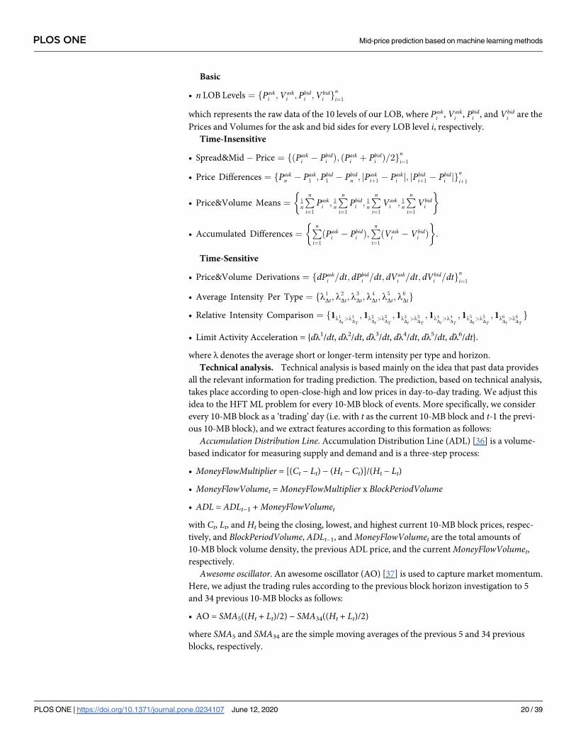
Basic

• n LOB Levels ¼ fPaski ;Vaski ; P

bidi ;V

bidi g

ni¼1

which represents the raw data of the 10 levels of our LOB, where Paski , Vaski , Pbidi , and Vbid

i are the

Prices and Volumes for the ask and bid sides for every LOB level i, respectively.

Time-Insensitive

• Spread&Mid � Price ¼ fðPaski � Pbidi Þ; ðP

aski þ P

bidi Þ=2g

ni¼1

• Price Differences ¼ fPaskn � Pask1; Pbid

1� Pbidn ; jP

askiþ1� Paski j; jP

bidiþ1� Pbidi jg

niþ1

• Price&Volume Means ¼ 1

n

Pn

i¼1

Paski ;1

n

Pn

i¼1

Pbidi ;1

n

Pn

i¼1

Vaski ;

1

n

Pn

i¼1

Vbidi

� �

• Accumulated Differences ¼Pn

i¼1

ðPaski � Pbidi Þ;

Pn

i¼1

ðVaski � V

bidi Þ

� �

.

Time-Sensitive

• Price&Volume Derivations ¼ fdPaski =dt; dPbidi =dt; dV

aski =dt; dV

bidi =dtg

ni¼1

• Average Intensity Per Type ¼ fl1

Dt; l2

Dt; l3

Dt; l4

Dt; l5

Dt; l6

Dtg

• Relative Intensity Comparison ¼ f1l1Dt>l1

DT; 1l2

Dt>l2

DT; 1l3

Dt>l3

DT; 1l4

Dt>l4

DT; 1l5

Dt>l5

DT; 1l6

Dt>l6

DTg

• Limit Activity Acceleration = {dλ1/dt, dλ2/dt, dλ3/dt, dλ4/dt, dλ5/dt, dλ6/dt}.

where λ denotes the average short or longer-term intensity per type and horizon.

Technical analysis. Technical analysis is based mainly on the idea that past data provides

all the relevant information for trading prediction. The prediction, based on technical analysis,

takes place according to open-close-high and low prices in day-to-day trading. We adjust this

idea to the HFT ML problem for every 10-MB block of events. More specifically, we consider

every 10-MB block as a ‘trading’ day (i.e. with t as the current 10-MB block and t-1 the previ-

ous 10-MB block), and we extract features according to this formation as follows:

Accumulation Distribution Line. Accumulation Distribution Line (ADL) [36] is a volume-

based indicator for measuring supply and demand and is a three-step process:

• MoneyFlowMultiplier = [(Ct − Lt) − (Ht − Ct)]/(Ht − Lt)

• MoneyFlowVolumet =MoneyFlowMultiplier x BlockPeriodVolume

• ADL = ADLt−1 +MoneyFlowVolumet

with Ct, Lt, and Ht being the closing, lowest, and highest current 10-MB block prices, respec-

tively, and BlockPeriodVolume, ADLt−1, andMoneyFlowVolumet are the total amounts of

10-MB block volume density, the previous ADL price, and the currentMoneyFlowVolumet,respectively.

Awesome oscillator. An awesome oscillator (AO) [37] is used to capture market momentum.

Here, we adjust the trading rules according to the previous block horizon investigation to 5

and 34 previous 10-MB blocks as follows:

• AO = SMA5((Ht + Lt)/2) − SMA34((Ht + Lt)/2)

where SMA5 and SMA34 are the simple moving averages of the previous 5 and 34 previous

blocks, respectively.




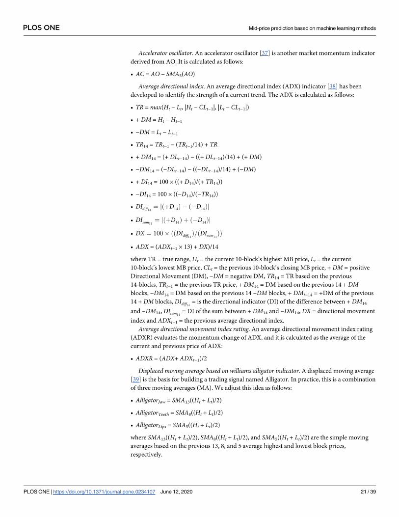
Accelerator oscillator. An accelerator oscillator [37] is another market momentum indicator

derived from AO. It is calculated as follows:

• AC = AO − SMA5(AO)

Average directional index. An average directional index (ADX) indicator [38] has been

developed to identify the strength of a current trend. The ADX is calculated as follows:

• TR =max(Ht − Lt, |Ht − CLt−1|, |Lt − CLt−1|)

• + DM =Ht −Ht−1

• −DM = Lt − Lt−1

• TR14 = TRt−1 − (TRt−1/14) + TR

• + DM14 = (+ DLt−14) − ((+ DLt−14)/14) + (+ DM)

• −DM14 = (−DLt−14) − ((−DLt−14)/14) + (−DM)

• + DI14 = 100 × ((+ D14)/(+ TR14))

• −DI14 = 100 × ((−D14)/(−TR14))

• DIdiff14¼ jðþD14Þ � ð� D14Þj

• DIsum14¼ jðþD14Þ þ ð� D14Þj

• DX ¼ 100� ððDIdiff14Þ=ðDIsum14

ÞÞ

• ADX = (ADXt−1 × 13) + DX)/14

where TR = true range,Ht = the current 10-block’s highest MB price, Lt = the current

10-block’s lowest MB price, CLt = the previous 10-block’s closing MB price, + DM = positive

Directional Movement (DM), −DM = negative DM, TR14 = TR based on the previous

14-blocks, TRt−1 = the previous TR price, + DM14 = DM based on the previous 14 + DMblocks, −DM14 = DM based on the previous 14 −DM blocks, + DMt−14 = +DM of the previous

14 + DM blocks, DIdiff14= is the directional indicator (DI) of the difference between + DM14

and −DM14, DIsum14= DI of the sum between + DM14 and −DM14, DX = directional movement

index and ADXt−1 = the previous average directional index.

Average directional movement index rating. An average directional movement index rating

(ADXR) evaluates the momentum change of ADX, and it is calculated as the average of the

current and previous price of ADX:

• ADXR = (ADX+ ADXt−1)/2

Displaced moving average based on williams alligator indicator. A displaced moving average

[39] is the basis for building a trading signal named Alligator. In practice, this is a combination

of three moving averages (MA). We adjust this idea as follows:

• AlligatorJaw = SMA13((Ht + Lt)/2)

• AlligatorTeeth = SMA8((Ht + Lt)/2)

• AlligatorLips = SMA5((Ht + Lt)/2)

where SMA13((Ht + Lt)/2), SMA8((Ht + Lt)/2), and SMA5((Ht + Lt)/2) are the simple moving

averages based on the previous 13, 8, and 5 average highest and lowest block prices,

respectively.




Absolute price oscillator. An absolute price oscillator (APO) belongs to the family of price

oscillators. It is a comparison between fast and slow exponential moving averages and is calcu-

lated as follows:

• Mt = (Ht + Lt)/2

• APO = EMA5(Mt) − EMA13(Mt)

where EMA5(Mt) and EMA13(Mt) are the exponential moving averages of range 5 and 13 peri-

ods, respectively, for the average of high and low prices of the current 10-MB block.

Aroon indicator. An Aroon indicator [40] is used as a measure of trend identification of an

underlying asset. More specifically, the indicator has two main bodies: the uptrend and down-

trend calculation. We calculate the Aroon indicator based on the previous twenty 10-MB

blocks for the highest-high and lowest-low prices, respectively, as follows:

• ArronUp ¼ ð20 � Hhigh20=20Þ � 100

• ArronDown ¼ ð20 � Llow20=20Þ � 100

whereHhigh20and Llow20

are the highest-high and lowest-low 20 previous 10-MB block prices,

respectively.

Aroon oscillator. An Aroon oscillator is the difference between AroonUp and AroonDownindicators, which makes their comparison easier:

• Arron Oscillator = AroonUp—AroonDown

Average true range. Average true range (ATR) [41] is a technical indicator which measures

the degree of variability in the market and is calculated as follows:

• ATR = (ATRt−1 × (N − 1)+ TR)/N

Here we use N = 14, where N is the number of the previous 10-TR values, and ATRt−1 is the

previous ATR 10-MB block price.

Bollinger bands. Bollinger bands [42] are volatility bands which focus on the price edges of

the created envelope (middle, upper, and lower band) and can be calculated as follows:

• BBmiddle = SMA20(CL)

• BBupper ¼ SMA20ðCLÞ þ BBstd20� 2

• BBlower ¼ SMA20ðCLÞ � BBstd20� 2

where BBmiddle, BBupper, and BBlower represent the middle, upper, and lower Bollinger bands,

SMA20(CL) represents the simple moving average of the previous twenty 10-block closing

prices, and BBstd20represents the standard deviation of the last twenty 10-MB blocks.

Ichimoku clouds. Ichimoku clouds [43] are ‘one glance equilibrium charts,’ which means

that the trader can easily identify a good trading signal and is possible since this type of indica-

tor contains dense information (i.e. momentum and trend direction). Five modules are used

in an indicator’s calculation:

• Conversion Line (Tenkan–sen) = (H9 + L9)/2

• Base Line (Kijun–sen) =H26 + L26

• Leading Span A (Senkou Span A) = (Conversion Line + Base line)/2

• Leading Span B (Senkou Span B) = (H52 + L52)/2




• Lagging Span (Chikou Span) = CL26

where H, L, and CL denote the highest, lowest, and closing prices of the 10-MB raw data,

respectively, where subscripts 9, 26, and 52 denote the past horizon of our trading rules,

respectively.

Chande momentum oscillator. A Chande momentum oscillator (CMO) [40] belongs to the

family of technical momentum oscillators and can monitor overbought and oversold situa-

tions. There are two modules in the calculation process:

• Su ¼X19

i¼1

CLi � 1CLt>CLt� 19

• Sd ¼X19

i¼1

CLi � 1CLt<CLt� 19

• CMO = 100 × (Su—Sd)/(Su + Sd)

where CLi is the 10-block’s closing price with i = 1, and CLt and CLt−19 are the current block’s

closing price and the 19 previous blocks’ closing prices, respectively.

Chaikin oscillator. The main purpose of a Chaikin oscillator [44] is to measure the momen-

tum of the accumulation distribution line as follows:

• MFM = (CLt − Lt) − (Ht − CLt)]/(Ht − Lt)

• MFV ¼ MFM �X10

j¼1

Vj

• ADL = ADLt−1 +MFM

• Chaikin Oscillator = EMA3(ADL)—EMA10(ADL)

whereMFM andMFV stand forMoney Flow Multiplier andMoney Flow Volume, respectively,

V is the volume of each of the trading events in the 10-block MB, and EMA3(ADL) and

EMA10(ADL) are the exponential moving average for the past 3 and 10 10-MB blocks,

respectively.

Chandelier exit. A Chandelier exit [45] is part of the trailing stop strategies based on the vol-

atility measured by the ATR indicator. It is separated based on the number of ATRs that are

below the 22-period high (long) or above the 22-period low (short) and is calculated as

follows:

• ChandelierLong =H22 − ATR22 × 3

• ChandelierShort = L22 + ATR22 × 3

whereH22 and L22 denote the highest and lowest prices for a period of 22 10-MB blocks, and

ATR22 are the ATR values for the 22 previous 10-MB blocks.

Center of gravity oscillator. The center of gravity oscillator (COG) [46] is a comparison of

current prices against older prices within a specific time window and is calculated as follows:

• Mt = (Ht + Lt)/2

• COG = −(Mt + r ×Mt−1)/(Mt +Mt−1)

whereMt is the current mid-price of the highest and lowest prices of each of the 10-MB blocks,

and r is a weight that increases according to the number of the previousMt−1 prices.




Donchian channels. The Donchian channel (DC) [47] is an indicator which bands the signal

and notifies the ML trader of a price breakout. There are three modules in the calculation

process:

• DCupper ¼ Hhigh20

• DClower ¼ Llow20

• DCmiddle ¼ ðHhigh20þ Llow20

Þ=2

whereHhigh20and Llow20

are the highest high and lowest low prices of the previous twenty

10-MB blocks.

Double exponential moving average. A double exponential moving average (DEMA) [48]

provides a smoothed average and offers a diminished amount of delays as follows:

• Mt = (Ht + Lt)/2

• DEMA = 2 × EMA20(Mt) − EMA20(EMA20(Mt))

where EMA20 is the exponential moving average of span 20 of the closing prices under the

10-MB block format.

Detrended price oscillator. A detrended price oscillator (DPO) is an indicator used for

short-term and long-term signal identification. The DPO eliminates cycles that are longer

than the MA horizon. On day-to-day trading, the closing prices are considered for the calcula-

tion, but here, we use the highest 10-MB block price as follows:

• DPO ¼ ðHhigh10=ð10þ 2ÞÞ � SMA10ðCLÞ.

Heikin-Ashi. Heikin-Ashi [49] is a candlestick method and is described as a visual technique

that eliminates irregularities:

• HeikinClose = (Ot +Ht + Lt + CLt)/4

• HeikinOpen = (Ot−1 + CLt−1)/2

• HeikinHigh =max(Ht, Ot−1, CLt−1)

• HeikinLow =min(Lt, Ot−1, CLt−1)

where Ot−1 and CLt−1 are the open and close prices of the previous 10-MB block.

Highest high and lowest low. Highest high and lowest low creates an envelope of the trading

signal for the last twenty 10-MB blocks:

• HighestHigh ¼ Hhigh20

• LowestLow ¼ Llow20

Hull MA. A Hull moving average is a weighted moving average that reduces the smoothing

lag effect by using the square root of the block period. It is calculated as follows:

• HULLMA ¼WMA ffiffiffi10p ðAHLÞð2�WMA5ðAHLÞ � WMA10ðAHLÞÞ

whereWMA5(AHL) andWMA10(AHL) denote the weighted moving average of the average

high and low 10-MB block for periods 5 and 10, respectively.

Internal bar strength. Internal bar strength (IBS) [50] is based on the position of the day’s

closing price in relation to the day’s range where we adjust this idea to the 10-MB block setup

as follows:




• IBS = (CLt − Lt)/(Ht − Lt).

Keltner channels. Keltner channels [51] are based on Bollinger bands. The main difference,

for this volatility-based indicator, is that it uses ATR instead of standard deviation, as follows:

• MiddleChannle ¼ EMA20AHL

• UpperChannel =MiddleChannel+ 2 × ATR10

• LowerChannel =MiddleChannel − 2 × ATR10.

Moving Average Convergence/Divergence Oscillator (MACD). A moving average conver-

gence/divergence oscillator [52] is a measure of the convergence and divergence of two mov-

ing averages and is calculated as follows:

• MACD = EMA12(AHL) − EMA26(AHL)

where AHL is the average of high and low prices for 12 and 26 previous 10-MB blocks, respec-

tively, with EMA12(AHL) and EMA26(AHL) as the exponential moving average of AHL of span

12 and 26, respectively.

Median price. Median price is an indicator which simplifies the price overview. We calcu-

late this indicator based on the 10-MB block highest and lowest average prices:

• Mediant = (Ht + Lt)/2

Momentum. A momentum (MOM) indicator measures the rate of change of the selected

time series. In our case, we calculate it based on closing prices:

• MOM = CLt − CLt−1.

Variable moving average. A variable moving average (VMA) [53] is a dynamic indicator

which acts as a variable-length moving average with volatility-adaptation capabilities. We cal-

culate VMA based on the efficiency ratio (ER) as follows:

• Direction = |CLt − CLt−3|

• Volatility ¼ 3�P3

ii¼1

jCLii � CLiiþ1j

• ER = Direction/Volatility

• VMA ¼X3

jj¼1

a� ERjj � CLjj

where α = 2/(N+ 1), for N = 3 previous 10-MB blocks, is the adaptive parameter.

Normalized average true range. A normalized average true range (NATR) normalizes the

average true range as follows:

• NATR = (ATR/CLt) × 100.

Percentage price oscillator. A percentage price oscillator (PPO) displays the convergence

and divergence of two moving averages and focuses on the percentage change of the larger

moving average, as follows:

• MACD = EMA12(AHL) − EMA26(AHL)

• PPO = (MACD/EMA26(AHL)) × 100.




Rate of change. Rate of change (ROC) measures the ascent or descent speed of the time

series change:

• ROC = (CLt − CLt−12/CLt−12) × 100.

Relative strength index. A relative strength index (RSI) [38] is a measure of the velocity and

magnitude of directional time series movements and is calculated as follows:

• CLd = CLt − CLt−1

• AG14 ¼X14

l¼1

CLdl1CLdt>CLdt� 1

• AL14 ¼X14

l¼1

CLdl1CLdt<CLdt� 1

• RelativeStrength = AG14/AL14

• RSI = 100 − 100/(1+ RelativeStrength)

where AG14 and AL14 denotes the average gain and loss of the last fourteen 10-MB blocks,

respectively.

Parabolic stop and reverse. Parabolic SAR (PSAR) [41] is a trend following indicator which

protects profits. There are two main modules for its calculation, the Rising SAR and the Falling

SAR, and they are calculated as follows:

• Rising SAR

• AF = Incremental increase of a predefined step

• EP ¼ HHigh5

• SAR = SARt−1 + AFt−1(EPt−1 − SARt−1)

• Falling SAR

• AF = Incremental increase of a predefined step

• EP ¼ LLow5

• SAR = SARt−1 − AFt−1(EPt−1 − SARt−1)

where AF is the acceleration factor, and EP is the extreme point

Standard deviation. Standard deviation is a measure of volatility. We calculate this indicator

based on the closing prices of every 10-MB block, as follows:

• Deviation = CLt − SMA10(CL)

• SASD ¼ffiffiffiffiffiffiffiffiffiffiffiffiffiffiffiffiffiffiffiffiffiffiffiffiffiffiSMA10ðSVDÞ

p

where SMA10(CL) is the simple moving average of the last 10 closing 10-MB prices, SASD is

the squared deviation of the SMA of the standard deviation (SVD) of the last 10 closing values

of our 10-MB blocks.

Stochastic relative strength index. A stochastic relative strength index (Stoch RSI) [40] is a

range-bound momentum oscillator which provides information for the RSI based on the clos-

ing prices in terms of high and low stock prices:

• StochRSI ¼ ðRSIcurr � RSILLow10Þ=ðRSIHHigh10

� RSILLow10Þ




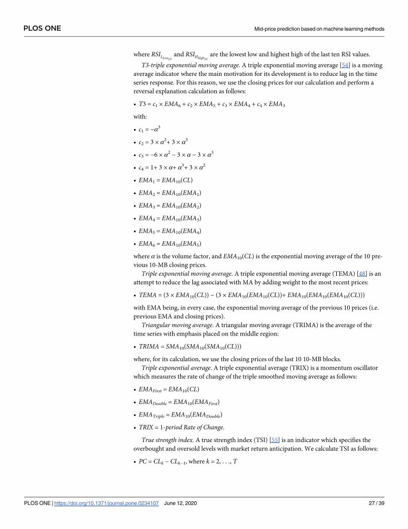
where RSILLow10and RSIHHigh10

are the lowest low and highest high of the last ten RSI values.

T3-triple exponential moving average. A triple exponential moving average [54] is a moving

average indicator where the main motivation for its development is to reduce lag in the time

series response. For this reason, we use the closing prices for our calculation and perform a

reversal explanation calculation as follows:

• T3 = c1 × EMA6 + c2 × EMA5 + c3 × EMA4 + c4 × EMA3

with:

• c1 = −α3

• c2 = 3 × α2+ 3 × α3

• c3 = −6 × α2 − 3 × α − 3 × α3

• c4 = 1+ 3 × α+ α3+ 3 × α2

• EMA1 = EMA10(CL)

• EMA2 = EMA10(EMA1)





where α is the volume factor, and EMA10(CL) is the exponential moving average of the 10 pre-

vious 10-MB closing prices.

Triple exponential moving average. A triple exponential moving average (TEMA) [48] is an

attempt to reduce the lag associated with MA by adding weight to the most recent prices:

• TEMA = (3 × EMA10(CL)) − (3 × EMA10(EMA10(CL))+ EMA10(EMA10(EMA10(CL)))

with EMA being, in every case, the exponential moving average of the previous 10 prices (i.e.

previous EMA and closing prices).

Triangular moving average. A triangular moving average (TRIMA) is the average of the

time series with emphasis placed on the middle region:

• TRIMA = SMA10(SMA10(SMA10(CL)))

where, for its calculation, we use the closing prices of the last 10 10-MB blocks.

Triple exponential average. A triple exponential average (TRIX) is a momentum oscillator

which measures the rate of change of the triple smoothed moving average as follows:

• EMAFirst = EMA10(CL)

• EMADouble = EMA10(EMAFirst)

• EMATriple = EMA10(EMADouble)

• TRIX = 1-period Rate of Change.

True strength index. A true strength index (TSI) [55] is an indicator which specifies the

overbought and oversold levels with market return anticipation. We calculate TSI as follows:

• PC = CLk − CLk−1, where k = 2, . . ., T




• APC = |CLk − CLk−1|, where k = 2, . . ., T

• EMA1 = EMA25(PC)


• EMA3 = EMA25(APC)


• TSI = 100 × EMA2/EMA4

where PC represents the closing price differences for the whole time series lookback period.

Ultimate oscillator. An ultimate oscillator (UO) [56] is a momentum oscillator indicator

with a multiple timeframe perspective. There are three main modules as presented in the fol-

lowing calculations:

• Average of seven 10-MB blocks

• BP ¼ CLt � ðCLt� 11CLt� 1<Ltþ Lt1CLt� 1>Lt

Þ

• TR1 ¼ CLt� 11CLt� 1>HtþHcurr1CLt� 1<Ht

• TR2 ¼ CLt� 11CLt� 1<Ltþ Lt1CLt� 1>Lt

• TR = TR1 + TR2

• Average7 ¼X7

l¼1

BPl=X7

l¼1

TRl

• Average of fourteen 10-MB blocks


Þ

• TR3 ¼ CLt� 11CLt� 1>HtþHt1CLt� 1<Ht


• TR = TR3 + TR4

• Average14 ¼X14

l¼1

BPl=X14

l¼1

TRl

• Average of twenty-eight 10-MB blocks


Þ

• TR5 ¼ CLt� 11CLt� 1>HtþHt1CLt� 1<Ht


• TR = TR5 + TR6

• Average28 ¼X28

l¼1

BPl=X28

l¼1

TRl

• UO = 100 × [(4 × Average7)+ (2 × Average14)+ Average28]/(4+ 2+ 1)

where BP represents buying pressure.




Weighted close. Weighted close (WCL) is the average of the four universal types of prices

which are included in each of our 10-MB blocks:

• WCL = (Ht + Lt+ 2 × CLt)/4.

Williams %R. Williams %R [56] is a momentum technical indicator which informs the ML

trader whether the market is trading close to the high or low trading range. It is calculated as

follows:

• %R ¼ � 100� ðHHigh14� CLtÞ=ðHHigh14

� LLow14Þ

where -100 corrects the inversion.

Zero-lag exponential moving average. Zero-lag exponential moving average (ZLEMA)

belongs to the EMA family of indicators where the main purpose is to reduce or remove the

impulse lag by introducing an error term. It is calculated as follows:

• error = CL − CLlag

• Input = CL+ error

• ZLEMA = EMA10(Input)

where lag = (N − 1)/2 with N = 1 in our case.

Fractals. A fractal [39] is an indicator used to detect top and bottom trends by focusing on

five consecutive blocks, which, in our case, are five 10-MB blocks used for two different

scenarios:

• Buy FractalsA buy fractal is a sequence of five consecutive 10-MB blocks where the highest high is pre-

ceded by two lower highs and is followed by two lower highs.

• Sell FractalsThe opposite framework is a sell fractal. 10-MB blocks can overlap in the quest of these two

types of fractals.

Here, we calculate fractals separately for the open, close, lowest, and highest 10-MB block

prices.

Linear regression line. Linear regression line (LRL) is a basic statistical method that provides

information for a future projection wherein trading is used to capture overextended price

trends. We perform LRL for each 10-MB block without any prior stationarity assumptions.

The basic calculations are as follows:

• PV = c1 + c2 ×MBprices

• c2 ¼ r � ðstdPV=stdMBpricesÞ

• r ¼

X10

i¼1

ðMBpricesðiÞ� MBprices ÞðPVðiÞ� PV Þ

!

� ffiffiffiffiffiffiffiffiffiffiffiffiffiffiffiffiffiffiffiffiffiffiffiffiffiffiffiffiffiffiffiffiffiffiffiffiffiffiffiffiffiffiffiffiffiffiffiffiffiffiffiffiffiffiffiffiffiffiffiffiffiP10

i¼1

ðMBpricesðiÞ� MBprices Þ2ðP10

i¼1

ðPVðiÞ� PV Þ2

�s

• c1 ¼ PV � c2 �MBprices

where PV are the predicted values, r is the correlation coefficient, andMBprices and PV are the

mean of 10-MB block prices and predicted values, respectively.




Digital filtering: Rational transfer function. A rational transfer function [57] is a representa-

tion of a linear time-invariant (LTI) filter, with the assumption that the input signal depends

on the time-frequency domain, which describes the input-output relationship of a signal. In

the Z-tranform domain, we have the following rational transfer function:

• O zð Þ ¼ bð1Þþbð2Þz� 1þ:::þbðnbþ1Þþz� nb1það2Þz� 1þ:::þaðnaþ1Þz� na IðzÞ,

where:

• I(z) and O(z) are the input (i.e. 10-MB block closing prices) and output respectively,

• b are the numerator coefficients,

• α are the denominator coefficients,

• na is the feedback order,

• nb is the feedforward order,

• z is the complex variable,

• the lookback period for the calculations is ten 10-MB blocks.

Digital filtering: Savitzky-golay filter. A Savitzky-Golay (S-G) digital filter [58, 59] is a dis-

crete convolution with a specific impulse response. We describe how the ML trader can obtain

the S-G signal based on higher degree polynomials:

• Least-Square Filter

• Objective: minimize error EN ¼Xm

i¼l

wiðyi �Xn

r¼0

prxri Þ2

• Partial derivative of the polynomial coefficients:

@Q@pk¼ 0!

Xm

i¼l

wiXn

r¼0

prxrþki ¼

Xm

i¼l

wiyixki

• Finite time series allow order summation change:

Xn

r¼0

prXm

i¼l

wixrþki ¼

Xm

i¼l

wiyixki

• As a result, the desired linear equations are the following:

Xm

i¼l

wix0i

Xm

i¼l

wix1i . . .

Xm

i¼l

wixniXm

i¼l

wix1i

Xm

i¼l

wix2i . . .

Xm

i¼l

wixnþ1i

..

. ... . .

. ...

Xm

i¼l

wixniXm

i¼l

wixnþ1i . . .

Xm

i¼l

wix2ni

2

66666666664

3

77777777775

p0

p1

..

.

pn

2

6664

3

7775¼

Xm

i¼l

wiyix0i

Xm

i¼l

wiyix1i

..

.

Xm

i¼l

wiyixni

2

66666666664

3

77777777775




equivalent to the notation A P = B where matrix A� 1 2 Rðnþ1Þ�ðnþ1Þunder the condition that

the polynomial degree is n�m − l.• S-G Filter

• Local convolution coefficients calculation

p0

p1

..

.

pn

2

666664

3

777775

¼

Xm

i¼l

wix0i . . .

Xm

i¼l

wixni

Xm

i¼l

wix1i . . .

Xm

i¼l

wixnþ1i

..

. . .. ..

.

Xm

i¼l

wixni . . .Xm

i¼l

wix2ni

2

66666666666664

3

77777777777775

� 1 Xm

i¼l

wiyix0i

Xm

i¼l

wiyix1i

..

.

Xm

i¼l

wiyixni

2

66666666666664

3

77777777777775

)

p0

p1

..

.

pn

2

666664

3

777775

¼

c0;0 c0;1 . . . c0;n

c1;0 c1;1 . . . c1;n

..

. ... . .

. ...

cn;0 cn;1 . . . cn;n

2

6666664

3

7777775

Xm

i¼l

wiyix0i

Xm

i¼l

wiyix1i

..

.

Xm

i¼l

wiyixni

2

66666666666664

3

77777777777775

• Response at the local point of 0 degree is:

y 0½ � ¼ c0;0 �Xm

i¼l

wiyix0

i þ c0;1 �Xm

i¼l

wiyix1

i þ :::þ c0;n �Xm

i¼l

wiyixni

Digital filtering: Zero-phase filter. A zero-phase filter [60] is a bidirectional filtering tech-

nique. With zero phase slope and even impulse response h(n), the filter provides an output sig-

nal, which is a zero phase recursive signal. This method is suitable for our experimental

protocol since we use training and testing sets rather than online learning architecture as we

will do in 4.2.4. The calculation process is as follows:

• Real Impulse response: h(n), n 2 Z

• Discrete-time Fourier Transformation:

HoTðhÞ ¼X1

n¼1

hðnÞcosðonTÞ � jX1

n¼1

hðnÞsinðonTÞ

• Based on Euler formula and h-even:HðejoTÞ ¼X1

n¼1

hðnÞcosðonTÞ

Remove offset and detrend. We present three detrend methods for short-term cycle isolation

and calculate them as follows:




• Remove Offset

• Offset ¼ CLt � ðXn

l¼1

CLlÞ=n

where n denotes the 10-MB lookback period

• Detrend—Least Squares Fitting Line

• R2 ¼Xn

i¼1

yi � gðxiÞ½ �2

•@ðR2Þ

@a¼ 0

•@ðR2Þ

@b ¼ 0

•a

b

" #

¼

nXn

i¼l

xi

Xn

i¼l

xiXn

i¼l

x2i

2

66664

3

77775

� 1 Xn

i¼l

yi

Xn

i¼l

xiyi

2

66664

3

77775

where α and b are the regression coefficients of g, and x represents the 10-MB closing prices.

Beta-like calculation. Beta [61] is a volatility indicator which considers market risk. We

adjust the notion of beta calculation to our experimental protocol where we index based on

the average of the closing prices (AvCL) with Avt as the current MB block price and Avt−1 as the

previous MB block’s closing price. Our calculations are as follow:

• IndexCL = CLt/CLt−1

• IndexAvCL ¼ Avt=Avt� 1

• DevCL = IndexCL − SMA10(IndexCL)

• DevAvCL ¼ IndexAvCL � SMA10ðIndexAvCLÞ

• Beta ¼ cov10ðDevCL;DevAvCLÞ=var10ðDevAvCLÞ

where cov10ðDevCL;DevAvCLÞ represents the covariance between the current closing price and

the average of the previous ten 10-MB closing prices, and var10ðDevAvCLÞ is the variance of the

sum of the ten previous IndexAvCL .Quantitative analysis. Quantitative analysis captures trading activity mainly via statistical

modelling. We focus on time series analysis, and more specifically, we examine features such

as autocorrelation and partial autocorrelation, among others (e.g., statistical tests), while at the

end of the section, we build an ML feature extraction method based on an online learning

setup and test the validity of our hypothesis.

Autocorrelation and partial correlation. Autocorrelation and partial correlation [62, 63] are

key features in the development of time series analysis. We treat our time series (i.e. stock

prices and log returns per 10-MB blocks) as stationary stochastic processes since we estimate

their local behavior based on 10-MB blocks:

• Autocorrelation

• ack ¼E ðzt � mÞðztþk � mÞ½ �ffiffiffiffiffiffiffiffiffiffiffiffiffiffiffiffiffiffiffiffiffiffiffiffiffiffiffiffiffiffiffiE ðzt � mÞ

2½ �E ðztþk � mÞ2½ �p




where zt and zt+ k are the time series of lag k, m ¼ E zt½ � ¼R1� 1zpðzÞdz and s2

z ¼

E ðzt � mÞ2

� �¼R1� 1ðz � mÞ2pðzÞdz are the constant mean and constant variance respectively.

• Partial Correlation

• For the general case of an autoregressive model AR(p), we have:

xi+ 1 = ϕ1 xi + ϕ2 xi−1+ . . .+ ϕp xi−p+ 1 + ξi+ 1 of lag 1 up to p follows:

• < xixiþ1 >¼Xp

j¼1

ð�j < xixi� jþ1 >Þ

• < xi� 1xiþ1 >¼Xp

j¼1

ð�j < xi� 1xi� jþ1 >Þ

• < xi� kþ1xiþ1 >¼Xp

j¼1

ð�j < xi� kþ1xi� jþ1 >Þ

• < xi� pþ1xiþ1 >¼Xp

j¼1

ð�j < xi� pþ1xi� jþ1 >Þ

by diving with N − 1 and autocovariance of zero separated periods (where the autocovariance

function is even), all the lag periods above will be:

• r1 ¼Xp

j¼1

�jrj� 1

• r2 ¼Xp

j¼1

�jrj� 2

• rk ¼Xp

j¼1

�jrj� k

• rp ¼Xp

j¼1

�jrj� p

where r1, r2, . . ., rk, rp can be described by the matrix operations RF = r, R 2 Rp�p, Φ 2 Rp�1

and r 2 Rp�1. The symmetric and full rank F are as follows: Φ ¼ R� 1r.

• Yule-Walker Equations calculation:

• Lag interval 1� i� p

• Φ ¼ ðRðiÞÞ� 1rðiÞ ¼

�1

�2

..

.

�i

2

6666664

3

7777775

Cointegration. We investigate time-series equilibrium [64, 65] by testing the cointegrated

hypothesis. Utilizing the cointegration test will help ML traders avoid the problem of spurious

regression. We employ the Engle-Granger (EG) test for the multivariable case of LOB ask (At)and bid (Bt) times series. We formulate the EG test for the ask and bid LOB prices as follows:

• At and Bt* I(d), where I(d) represents the order of integration




• Cointegration equation based on the error term: ut = At − αBt

• EG Hypothesis: u(t)* I(d), d 6¼ 0

• Perform ordinary leat squares (OLS) for the estimation of a and unit root test for:

u ¼ At � aBt

Order book imbalance. We calculate the order book imbalance [4] based on the volume

depth of our LOB as follows:

• VI ¼ Vbl � Val

Vbl þVal

where Val and Vb

l are the volume sizes for the ask and bid LOB sides at level l.

Additional results

Tables 5–9 are provided below:

Feature sorting lists

These are the five sorted lists of the 273 hand-crafted features. A detailed feature name list

follows.

1. Features sorting list based on Entropy:

{218;161;170;160;166;206;209;196;199;197;193;174;182;183;146;157;171;172;173;156;155;

184;194;137;177;176;138;195;136;217;213;181;147;245;243;247;188;241;242;244;240;246;

255;248;249;189;210;265;211;226;236;225;235;221;231;223;233;222;232;214;169;220;230;

228;238;224;234;83;84;227;237;139;135;134;142;162;140;185;129;86;128;186;212;141;250;

261;16;20;262;207;153;14;81;12;208;260;4;18;10;259;24;196;2;163;150;187;82;28;192;22;8;

26;6;32;30;36;34;40;148;175;154;149;38;151;60;59;58;57;56;55;54;53;52;51;198;215;216;158;

167;159;168;152;164;100;102;21;25;29;13;17;9;5;33;1;23;19;15;27;11;31;37;7;3;35;85;39;104;

252;96;98;106;269;108;92;112;110;88;253;116;124;120;145;94;50;90;180;256;114;49;165;118;

123;122;48;126;268;119;115;80;47;111;143;144;46;107;70;45;125;103;121;44;117;43;113;99;

42;109;254;270;271;105;41;95;101;91;272;97;273;93;179;69;178;87;68;79;89;127;67;78;201;

191;66;133;77;65;76;205;203;61;200;202;71;75;62;72;64;206;204;257;63;132;131;74;73;130;

251;258;267;266;219;229;239;263;264}

2. Features sorting list based on LMS1:

{266;4;6;87;1;209;267;268;218;254;251;92;253;250;91;252;255;193;122;270;174;183;267;108;

103;32;18;147;216;100;118;263;264;111;41;90;112;20;273;24;127;116;120;109;110;126;225;

235;164;107;98;102;124;165;89;94;133;114;119;104;96;95;88;115;188;61;93;125;101;97;105;

113;208;211;99;180;121;117;246;106;123;189;248;228;238;8;210;186;130;185;10;14;242;157;

136;16;249;240;244;65;66;64;69;153;28;73;22;170;143;142;184;178;30;154;76;79;67;75;63;74;

78;256;247;245;146;219;229;239;68;187;62;70;176;201;179;194;72;197;131;132;77;217;42;43;

44;45;46;47;48;49;50;71;85;207;40;258;226;236;80;260;262;134;135;36;204;144;145;38;26;12;

84;199;195;182;215;156;171;158;151;167;148;161;168;191;152;159;160;149;150;141;198;169;

166;2;212;213;181;3;5;7;9;11;13;15;17;19;21;23;25;27;29;31;33;35;37;39;51;52;53;54;55;56;57;

58;59;60;81;82;86;155;163;196;175;214;272;172;173;140;190;192;139;200;162;227;237;222;

232;220;230;241;243;224;234;271;206;34;83;177;205;203;221;223;231;233;202;138;137;261;

128;129;257;259;265}




3. Features sorting list based on LMS2:

{269;257;262;81;127;128;41;142;181;205;203;259;223;202;200;199;243;273;176;206;256;204;

265;132;10;2;14;84;170;78;240;226;182;157;61;80;242;217;49;70;50;207;165;150;164;93;87;

62;43;89;66;215;18;154;251;111;222;8;261;201;258;270;271;65;96;151;216;272;210;186;124;

120;153;94;187;92;211;117;109;101;162;166;29;213;184;185;198;195;129;146;191;192;193;

196;174;171;159;149;161;139;125;113;106;102;266;118;104;218;36;38;156;190;250;63;85;

133;12;121;90;34;40;175;91;248;241;227;245;152;130;189;178;214;136;137;158;224;225;112;

99;115;264;212;169;141;163;220;221;188;197;194;209;208;168;22;105;114;110;268;16;23;

177;140;119;123;100;126;122;260;244;246;134;135;131;56;103;173;167;6;228;47;97;255;107;

180;71;155;4;254;253;179;82;138;32;28;143;252;116;30;144;147;88;108;73;95;98;249;20;51;

160;247;55;59;5;148;42;7;76;31;54;3;145;77;46;19;231;48;17;15;83;232;21;45;52;230;236;37;1;

24;58;69;13;53;35;67;172;33;183;79;86;26;267;75;219;25;234;9;44;39;11;229;237;57;235;239;

60;27;68;64;74;233;238;72;263}

4. Features sorting list based on LDA1:

{269;6;88;43;240;210;265;209;206;9;252;251;253;268;8;108;114;174;193;254;100;263;264;

110;186;273;216;90;99;122;185;92;183;267;16;225;235;14;103;119;112;107;95;104;147;111;

91;115;270;127;109;116;120;18;89;94;118;126;98;180;106;208;250;124;96;188;113;125;121;

153;123;105;117;93;97;101;248;242;61;133;189;87;102;211;145;66;65;64;69;136;184;142;73;

76;157;75;74;78;67;63;79;170;178;77;219;229;239;262;182;130;245;70;22;194;244;24;12;266;

84;247;167;173;146;60;207;59;17;33;196;158;165;4;218;25;149;203;3;36;53;37;86;21;30;155;

58;164;48;246;161;223;26;85;226;205;41;144;80;47;15;135;179;152;27;160;39;38;81;241;50;

236;40;220;7;204;260;83;143;258;168;166;51;141;162;23;57;19;131;10;42;132;82;56;49;62;

154;128;5;228;259;55;181;191;163;156;187;272;213;224;52;46;35;1;54;234;169;150;255;227;

45;238;31;201;192;190;199;261;172;44;134;2;140;129;20;72;214;215;195;68;151;271;198;237;

171;11;29;137;221;222;32;13;217;148;230;232;231;233;197;28;159;249;139;212;256;176;177;

243;71;200;34;138;175;202;257}

5. Features sorting list based on LDA2:

{272;269;150;

143;262;2;259;83;87;71;129;205;204;120;6;48;248;141;179;203;212;139;184;43;144;118;79;

177;18;52;8;193;132;110;70;191;100;103;146;241;138;206;252;247;273;63;211;207;22;10;142;

244;16;258;122;221;219;108;217;47;93;140;40;180;202;34;256;4;115;96;218;134;102;99;270;

111;253;66;189;88;90;94;36;199;12;75;254;243;72;137;45;265;64;251;77;222;155;255;210;

104;209;174;267;105;194;50;14;126;109;32;170;200;125;98;127;89;227;44;201;119;28;245;61;

65;268;192;216;112;20;186;42;250;187;107;121;116;84;185;128;30;237;156;124;160;195;133;

147;41;223;215;123;113;135;173;148;271;214;169;131;232;39;149;35;178;68;190;31;198;106;

157;188;38;260;168;153;228;55;5;69;246;114;67;15;266;76;152;33;183;37;27;238;46;242;17;

166;101;54;23;117;58;56;11;167;261;9;91;162;29;7;97;163;151;233;57;78;24;95;86;225;164;

220;154;181;249;171;230;229;130;172;60;26;182;51;1;3;136;159;25;59;208;145;85;53;80;224;

92;240;13;81;231;175;264;197;257;74;158;234;213;196;176;235;19;21;263;165;82;226;236;73;

161;239;62;49}

Detailed feature list:

{1-40:Raw LOB Levels, 41-60:Spread & Mid-Price, 61-80:Price Differences, 81-84:Price &

Volume Means, 85-86:Accumulated Differences, 87-126:Price & Volume Derivations, 127-

132:Average Intensity Per Type, 132-136:Relative Intensity Comparison & Limit Activity

Acceleration LOB features: Some of the trade types in Relative Intensity Comparison and

Limit Activity Acceleration features do not appear in the Nordic dataset., 137:Accumulation

Distribution Line, 138:Awesome Oscillator, 139:Accelerator Oscillator, 140:Average




Directional Index, 141:Average Directional Movement Index Rating, 142:AlligatorsJaw, 143:

AlligatorsTeeth, 144:AlligatorsLips, 145:Absolute Price Oscillator, 146:Aroon Indicator/

AroonUp, 147:Aroon Indicator/AroonDown, 148:Aroon Oscillator, 149:Average True Range,

150:Bollinger Bands,151:Ichimoku Clouds/Tenkan sen, 152:Ichimoku Clouds/Kijun sen, 153:

Ichimoku Clouds/Senkou Span, 154:Ichimoku Clouds/Senkou Span 52-Period, 155:Ichimoku

Clouds/Chickou Span, 156:Chande Momentum Oscillator, 157:Chaikin Oscillator, 158:Chan-

delier Exit Long, 159:Chandelier Exit Short, 160:Center of Gravity Oscillator, 161:Donchian

Channels/Upper Channel, 162:Donchian Channels/Lower Channel, 163:Donchian Channels/

Middle Channel, 164:Double Exponential Moving Average, 165:Detrended Price Oscillator,

166:Heikin Ashi Close, 167:Heikin Ashi Open, 168:Heikin Ashi High, 169:Heikin Ashi Low,

170:Highest High, 171:Lowest Low, 172:Hull Moving Average, 173:Internal Bar Strength, 174:

Keltern Channels/Lower Channel, 175:Keltern Channels/Middle Line, 176:Keltern Channels/

Upper Channel, 177:Moving Average Convergence Divergence, 178:Median Price based on

High and Low, 179:Positive Directional Index, 180:Negative Directional Index, 181:Positive

Directional Index, 182:Positive Directional Movement, 183:Negative Directional Movement,

184:Momentum, 185:Variable Moving Average, 186:Normalized Average True Range, 187:

Percentage Price Oscillator/Moving Average Convergence Divergence, 188:Percentage Price

Oscillator, 189:Rate of Change, 190:Relative Strength Index, 191:Relative Strength Index with-

out the 100th extreme case, 192:Parabolic Stop And Reverse/Rising Stop And Reverse, 193:Par-

abolic Stop And Reverse/Folliwng Stop And Reverse:, 194:Standard Deviation, 195:Stochastic

Relative Strength Index, 196:T3 Triple Exponential Moving Average, 197:Triple Exponential

Moving Average, 198:Triangular Moving Average, 199:Triple Exponential Average, 200:True

Strength Index, 201:Ultimate Oscillator, 202:Weighted Close Price, 203:Williams %R, 204:

Weighted Moving Average, 205:Fractals, 206:Linear Regression Line/Regression Coefficient,

207:Linear Regression Line/Intercept, 208:Linear Regression Line/Slope, 209:Linear Regres-

sion Line/Correlation Coefficient, 210:Linear Regression Line/R-squared, 211:Digital Filter-

ing/Rational Transfer Function, 212:Digital Filtering/Low-Pass Savitzky-Golay Filter, 213:

Zero-Phase digital filtering, 214:Remove Offset, 215:Remove Baseline, 216:Detrend, 217:Beta

like Calculation, 218—254:Autocorrelation & Partial Autocorrelation for LOB Levels, 255:

Correlation Between Price and Volume, 256:Bollinger Bands, 257—258:Cointegration Test/h

Values, 259-260:Cointegration Test/p values, 261-262:Cointegration Test/Statistics, 263-264:

Cointegration Test/C Values, 265:Order Book Imbalance, 266—273:Logistic Regression.}

Acknowledgments

The authors wish to acknowledge CSC-IT Center for Science, Finland, for generous computa-

tional resources.

Author Contributions

Supervision: Juho Kanniainen, Moncef Gabbouj, Alexandros Iosifidis.

Writing – original draft: Adamantios Ntakaris.

References1. Dash R, Dash PK. A hybrid stock trading framework integrating technical analysis with machine learning

techniques. The Journal of Finance and Data Science. 2016; 2(1):42–57. https://doi.org/10.1016/j.jfds.

2016.03.002

2. Gould MD, Porter MA, Williams S, McDonald M, Fenn DJ, Howison SD. Limit order books. Quantitative

Finance. 2013; 13(11):1709–1742. https://doi.org/10.1080/14697688.2013.803148



https://doi.org/10.1016/j.jfds.2016.03.002

https://doi.org/10.1016/j.jfds.2016.03.002

https://doi.org/10.1080/14697688.2013.803148


3. Passalis N, Tsantekidis A, Tefas A, Kanniainen J, Gabbouj M, Iosifidis A. Time-series classification

using neural bag-of-features. IEEE 25th European Conference of Signal Processing; 2017. p. 301–305,

2017.

4. Sirignano JA. Deep learning for limit order books. Quantitative Finance. 2019; 19(4):549–570. https://

doi.org/10.1080/14697688.2018.1546053

5. Thanh DT, Kanniainen J, Gabbouj M, Iosifidis A. Tensor representation in high-frequency financial data

for price change prediction. arXiv:170901268. 2017;.

6. Tsantekidis A, Passalis N, Tefas A, Kanniainen J, Gabbouj M, Iosifidis A. Forecasting stock prices from

the limit order book using convolutional neural networks. IEEE 19th Conference on Business Informat-

ics. vol. 1; 2017. p. 7-12, 2017.

7. Tsantekidis A, Passalis N, Tefas A, Kanniainen J, Gabbouj M, Iosifidis A. Using deep learning to detect

price change indications in financial markets. IEEE 25th European Conference of Signal Processing;

2017. p. 2511–2515, 2017.

8. Ntakaris A, Mirone G, Kanniainen J, Gabbouj M, Iosifidis A. Feature Engineering for Mid-Price Predic-

tion With Deep Learning. IEEE Access. 2019; 7:82390–82412. https://doi.org/10.1109/ACCESS.2019.

2924353

9. Chandrashekar G, Sahin F. A Survey on Feature Selection Methods. Comput Electr Eng. 2014; 40

(1):16–28. https://doi.org/10.1016/j.compeleceng.2013.11.024

10. Miao J, Niu L. A survey on feature selection. Procedia Computer Science. 2016; 91:919–926. https://

doi.org/10.1016/j.procs.2016.07.111

11. Battiti R. Using mutual information for selecting features in supervised neural net learning. IEEE Trans-

actions on neural networks. 1994; 5(4):537–550. https://doi.org/10.1109/72.298224 PMID: 18267827

12. Liu H, Sun J, Liu L, Zhang H. Feature selection with dynamic mutual. information. Pattern Recognition.

2009; 42(7):1330–1339. https://doi.org/10.1016/j.patcog.2008.10.028

13. Murphy JJ. Technical Analysis of the Financial Markets: A Comprehensive Guide to Trading Methods

and Applications. New York Institute of Finance Series. New York Institute of Finance; 1999. Available

from: https://books.google.fi/books?id=5zhXEqdr_IcC.

14. Scholtus ML, van Dijk DJ. High-frequency technical trading: The importance of speed. Available at

SSRN: https://ssrncom/abstract=2013789. 2012;.

15. Kablan A, Ng W. High frequency trading using fuzzy momentum analysis. Proceedings of the World

Congress on Engineering. vol. 1; 2010.

16. Patel J, Shah S, Thakkar P, Kotecha K. Predicting stock and stock price index movement using Trend

Deterministic Data Preparation and machine learning techniques. Expert Systems with Applications.

2015; 42(1):259–268. https://doi.org/10.1016/j.eswa.2014.07.040

17. Chan LKC, Karceski J, Lakonishok J. On Portfolio Optimization: Forecasting Covariances and Choos-

ing the Risk Model. The Review of Financial Studies. 1999; 12(5):937–974. https://doi.org/10.1093/rfs/

12.5.937

18. Perold AF. Large-Scale Portfolio Optimization. Management Science. 1984; 30(10):1143–1160. https://

doi.org/10.1287/mnsc.30.10.1143

19. Fama EF. Risk, return and equilibrium: some clarifying comments. The Journal of Finance. 1968; 23

(1):29–40. https://doi.org/10.1111/j.1540-6261.1968.tb02996.x

20. Sharpe WF. Capital asset prices: A theory of market equilibrium under conditions of risk. The Journal of

Finance. 1964; 19(3):425–442. https://doi.org/10.2307/2977928

21. Diebold FX, Hahn J, Tay AS. Multivariate Density Forecast Evaluation and Calibration In Financial Risk

Management: High-Frequency Returns on Foreign Exchange. The Review of Economics and Statistics.

1999; 81(4):661–673. https://doi.org/10.1162/003465399558526

22. Smith CW, Smithson CW, Wilford DS. Managing Financial Risk. Journal of Applied Corporate Finance.

1989; 1(4):27–48. https://doi.org/10.1111/j.1745-6622.1989.tb00172.x

23. Iosifidis A, Tefas A, Pitas I. Multidimensional sequence classification based on fuzzy distances and dis-

criminant analysis. IEEE Transactions on Knowledge and Data Engineering. 2012; 25(11):2564–2575.

https://doi.org/10.1109/TKDE.2012.223

24. Taylor SJ. Modelling financial time series. World Scientific; 2008.

25. Shen S, Jiang H, Zhang T. Stock market forecasting using machine learning algorithms. Department of

Electrical Engineering, Stanford University, Stanford, CA, Available at: https://

wwwsemanticscholarorg/paper/Stock-Market-Forecasting-Using-Machine-Learning-Shen-Jiang/

b68e8d2f4d2c709bb5919b82effcb6a7bbd3db37. 2012; p. 1–5.

26. Poterba JM, Summers LH. Mean reversion in stock prices: Evidence and implications. Journal of finan-

cial economics. 1988; 22(1):27–59. https://doi.org/10.1016/0304-405X(88)90021-9



https://doi.org/10.1080/14697688.2018.1546053

https://doi.org/10.1080/14697688.2018.1546053

https://doi.org/10.1109/ACCESS.2019.2924353

https://doi.org/10.1109/ACCESS.2019.2924353

https://doi.org/10.1016/j.compeleceng.2013.11.024

https://doi.org/10.1016/j.procs.2016.07.111

https://doi.org/10.1016/j.procs.2016.07.111

https://doi.org/10.1109/72.298224

http://www.ncbi.nlm.nih.gov/pubmed/18267827

https://doi.org/10.1016/j.patcog.2008.10.028

https://books.google.fi/books?id=5zhXEqdr_IcC

https://ssrncom/abstract=2013789

https://doi.org/10.1016/j.eswa.2014.07.040

https://doi.org/10.1093/rfs/12.5.937

https://doi.org/10.1093/rfs/12.5.937

https://doi.org/10.1287/mnsc.30.10.1143

https://doi.org/10.1287/mnsc.30.10.1143

https://doi.org/10.1111/j.1540-6261.1968.tb02996.x

https://doi.org/10.2307/2977928

https://doi.org/10.1162/003465399558526

https://doi.org/10.1111/j.1745-6622.1989.tb00172.x

https://doi.org/10.1109/TKDE.2012.223

https://wwwsemanticscholarorg/paper/Stock-Market-Forecasting-Using-Machine-Learning-Shen-Jiang/b68e8d2f4d2c709bb5919b82effcb6a7bbd3db37



https://doi.org/10.1016/0304-405X(88)90021-9


27. Fang Y, Xu D. The predictability of asset returns: an approach combining technical analysis and time

series forecasts. International Journal of Forecasting. 2003; 19(3):369–385. https://doi.org/10.1016/

S0169-2070(02)00013-4

28. Kercheval AN, Zhang Y. Modelling high-frequency limit order book dynamics with support vector

machines. Quantitative Finance. 2015; 15(8):1315–1329. https://doi.org/10.1080/14697688.2015.

1032546

29. Ntakaris A, Magris M, Kanniainen J, Gabbouj M, Iosifidis A. Benchmark dataset for mid-price forecast-

ing of limit order book data with machine learning methods. Journal of Forecasting. 2018; 37(8):852–

866. https://doi.org/10.1002/for.2543

30. Broomhead DS, Lowe D. Radial basis functions, multi-variable functional interpolation and adaptive net-

works. Royal Signals and Radar Establishment Malvern (United Kingdom); 1988.

31. Iosifidis A, Tefas A, Pitas I. On the kernel extreme learning machine classifier. Pattern Recognition Let-

ters. Pattern Recognition Letters. 2015; 54:11–17. https://doi.org/10.1016/j.patrec.2014.12.003

32. Richman JS, Moorman JR. Physiological time-series analysis using approximate entropy and sample

entropy. American Journal of Physiology-Heart and Circulatory Physiology. 2000; 278(6):H2039–

H2049. https://doi.org/10.1152/ajpheart.2000.278.6.H2039 PMID: 10843903

33. Huang GB, Zhu QY, Siew CK. Extreme learning machine: theory and applications. Neurocomputing.

2006; 70(1-3):489–501. https://doi.org/10.1016/j.neucom.2005.12.126

34. Zhang K, Kwok JT, Parvin B. Prototype vector machine for large scale semi-supervised learning. Pro-

ceedings of the 26th Annual International Conference on Machine Learning. ACM; 2009. p. 1233–1240.

35. Iosifidis A, Tefas A, Pitas I. Approximate kernel extreme learning machine for large scale data classifica-

tion. Neurocomputing. 2017; 219:210–220. https://doi.org/10.1016/j.neucom.2016.09.023

36. Chua S. Sammy Chua’s Day Trade Your Way to Financial Freedom. John Wiley & Sons; 2006.

37. Williams B. New trading dimensions: how to profit from chaos in stocks, bonds, and commodities. vol.

72, 1998. John Wiley & Sons; 1.

38. Wilder JW Jr. The Relative Strength Index. Journal of Technical Analysis of Stocks and Commodities.

1986; 4:343–346.

39. Gregory-Williams J, Williams BM. TTrading chaos: maximize profits with proven technical techniques.

vol. 172, 2012. John Wiley & Sons; 2012.

40. Chande TS, Kroll S. The new technical trader. New York. 1994;.

41. Wilder JW. New concepts in technical trading systems. Trend Research; 1978.

42. Bollinger J. Bollinger on Bollinger bands. McGraw Hill Professional; 2001.

43. Muranaka K. Ichimoku Charts. Technical Analysis of Stocks and Commodities–Magazine Edition.

2000; 18(10):22–31.

44. Naiman E. Small encyclopedia of trader. Moscow: Alpina Business Books. 2009; 456.

45. Elder A. Come into my trading room: A complete guide to trading. vol. 163, 2002. John Wiley & Sons;

2002.

46. Ehlers JF. Rocket science for traders: digital signal processing applications. vol. 112, 2001. John Wiley

& Sons; 2001.

47. Rayome DL, Jain A, Konku D. Technical Analysis: Donchian Channels and the British Pound. IABE-

Annual Conference; 2007. p. 302, 2007.

48. Mulloy PG. Smoothing data with faster moving averages. Stocks & Commodities. 1994; 12(1):11–19.

49. Valcu D. Using The Heikin-Ashi Technique. Available from: Technical Analysis of Stocks and Commodi-

ties–Magazine Edition. 2004; 22(2):16–29.

50. Pagonidis AS. The IBS Effect: Mean Reversion in Equity ETFs; 2014. http://www.naaim.org/wp-

content/uploads/2014/04/00V_Alexander_Pagonidis_The-IBS-Effect-Mean-Reversion-in-Equity-

ETFs-1.pdf.

51. Keltner CW. How to make money in commodities. Keltner Statistical Service; 1960.

52. Aspray T. Individual stocks and MACD. Technical Analysis of Stocks & Commodities. 1989; 7(2):56–

61.

53. Chande TS. Adapting moving averages to market volatility. Stock & Commodities. 1992; 10:3.

54. Tillson T. Better Moving Averages. Digital Filters. Monterrey; 1998.

55. Blau W. Double smoothed-stochastics. Technical Analysis of Stocks and Commodities. 1991; 9.

56. Williams L. The Ultimate Oscillator. Technical Analysis of Stocks and Commodities. 1985; 3(4):140–

141.



https://doi.org/10.1016/S0169-2070(02)00013-4

https://doi.org/10.1016/S0169-2070(02)00013-4

https://doi.org/10.1080/14697688.2015.1032546

https://doi.org/10.1080/14697688.2015.1032546

https://doi.org/10.1002/for.2543

https://doi.org/10.1016/j.patrec.2014.12.003

https://doi.org/10.1152/ajpheart.2000.278.6.H2039

http://www.ncbi.nlm.nih.gov/pubmed/10843903

https://doi.org/10.1016/j.neucom.2005.12.126

https://doi.org/10.1016/j.neucom.2016.09.023

http://www.naaim.org/wp-content/uploads/2014/04/00V_Alexander_Pagonidis_The-IBS-Effect-Mean-Reversion-in-Equity-ETFs-1.pdf




57. Kumaresan R. Identification of rational transfer function from frequency response sample. IEEE Trans-

actions on Aerospace and Electronic Systems. 1990; 26(6):925–934. https://doi.org/10.1109/7.62245

58. Savitzky A, Golay MJ. Smoothing and differentiation of data by simplified least squares procedures.

Analytical chemistry. 1964; 36(8):1627–1639. https://doi.org/10.1021/ac60214a047

59. Schafer RW. What Is a Savitzky-Golay Filter? IEEE Signal Processing Magazine. 2011; 28(4):111–

117. https://doi.org/10.1109/MSP.2011.941097

60. Smith SW. The scientist and engineer’s guide to digital signal processing. California Technical Pub.;

1999.

61. French CW. The Treynor capital asset pricing model. Journal of Investment Management. 2003;

1(2):60–72.

62. Box GE, Jenkins GM, Reinsel GC, Ljung GM. Time series analysis: forecasting and control. John Wiley

& Sons; 2015.

63. Eshel G. The Yule-Walker equations for the AR coefficients. Internet resource. 2003; 2:68–73.

64. Hamilton JD. Time series analysis. vol. 2. Princeton University Press Princeton; 1994.

65. Engle RF, Granger CWJ. Co-Integration and Error Correction: Representation, Estimation, and Testing.

Econometrica. 1987; 55(2):251–276. https://doi.org/10.2307/1913236



https://doi.org/10.1109/7.62245

https://doi.org/10.1021/ac60214a047

https://doi.org/10.1109/MSP.2011.941097

https://doi.org/10.2307/1913236


Mid-price prediction based on machine learning methods with ...

Documents

Transcript of Mid-price prediction based on machine learning methods with ...