Machine Learning Models using the COMPASS Data
249
Phenotyping Risk Profiles of Substance Use and Exploring the Dynamic Transitions in Use Patterns: Machine Learning Models using the COMPASS Data by Yang Yang A thesis presented to the University of Waterloo in fulfillment of the thesis requirement for the degree of Doctor of Philosophy in Public Health and Health Systems Waterloo, Ontario, Canada, 2021 ©Yang Yang 2021
-
Upload
khangminh22 -
Category
Documents
-
view
0 -
download
0
Transcript of Machine Learning Models using the COMPASS Data
Phenotyping Risk Profiles of Substance
Use and Exploring the Dynamic
Transitions in Use Patterns: Machine
Learning Models using the COMPASS
Data
by
Yang Yang
A thesis
presented to the University of Waterloo
in fulfillment of the
thesis requirement for the degree of
Doctor of Philosophy
in
Public Health and Health Systems
Waterloo, Ontario, Canada, 2021
©Yang Yang 2021

ii
EXAMINING COMMITTEE MEMBERSHIP
The following served on the Examining Committee for this thesis. The decision of the Examining
Committee is by majority vote.
Supervisor(s): Helen H. Chen
Professor of Practice
School of Public Health Sciences
Faculty of Health
Zahid A. Butt
Assistant Professor
School of Public Health Sciences
Faculty of Health
Internal Member(s): Plinio P. Morita
Associate Professor
School of Public Health Sciences
Faculty of Health
Scott T. Leatherdale
Professor
School of Public Health Sciences
Faculty of Health
Internal-External Member: Alexander Wong
Professor
Systems Design Engineering
External Examiner: Laura Rosella
Associate Professor
Dalla Lana School of Public Health
University of Toronto

iii
AUTHOR'S DECLARATION
I hereby declare that I am the sole author of this thesis. This is a true copy of the thesis, including any
required final revisions, as accepted by my examiners.
I understand that my thesis may be made electronically available to the public.
iv
Abstract
Background
Polysubstance use is on the rise among Canadian youth. Examining risk profiles and understanding
how the transition occurs in use patterns can inform the design and implementation of polysubstance
risk reduction intervention. The COMPASS study is longitudinal research examining health-related
behaviours among Canadian secondary school students, capturing data from multiple sources.
Machine learning (ML) techniques can reveal non-linearity and multivariate couplings associated
with population-level longitudinal data to inform public health policies.
Objectives
The overarching goal of this thesis is to identify phenotypes of risk profiles of youth polysubstance
use and examine the dynamic transitions of use patterns across time, utilizing both unsupervised ML
methods and a latent variable modelling approach. This thesis also aims to understand how ML
techniques are best used in modelling transitions and discovering the “hidden” patterns from large
complex population-based health survey data, using the COMPASS dataset as a showcase.
Methods
A linked sample (N = 8824) of three annual waves of the COMPASS data collected starting from the
school year of 2016-17 was used. Multiple imputations for missing values were performed. Substance
use indicators, including cigarette smoking, e-cigarette use, alcohol drinking, and marijuana
consumption, were categorized into “never use,” “occasional use,” and “current use.” To examine
phenotypes of risk profiles, hierarchical clustering, partitioning around medoids (PAM), and fuzzy
clustering algorithms were applied. The Boruta algorithm was used to identify a subset of features for
cluster analysis. Both the internal and external indices were employed to evaluate the clustering
validity. A multivariate latent Markov model (LMM) was implemented to explore the dynamic
transitions of use patterns over time. The least absolute shrinkage and selection operator (LASSO)
approach was applied to select the appropriate covariates for entering the LMM. Model selection was
based on the Bayesian information criterion (BIC) and the goodness-of-fit test.
Results

v
The top factors impacting youth polysubstance use included the number of smoking friends, the
number of skipped classes, the weekly money to spend/save oneself, and others. Four risk profiles of
polysubstance use were identified across the three waves: low, medium-low, medium-high, and high-
risk profiles. The heterogeneity in the prevalence and phenotype across these four risk profiles was
confirmed. The internal measures of clustering performance measured by average silhouette width
ranged from 0.51 to 0.55 across the three waves using different clustering algorithms. The clustering
algorithms achieved a relatively high degree of agreement on cluster membership. Comparing the
fuzzy (FANNY) clustering with PAM clustering, the adjusted Rand indices were 0.9698, 0.7676, and
0.6452 for the three waves. Four distinct use patterns were identified: no use (S1), occasional single-
use of alcohol (S2), dual-use of e-cigarette and alcohol (S3), and current multi-use (S4). The initial
probabilities of each subgroup were 0.5887, 0.2156, 0.1487, and 0.0470. The marginal distribution of
S1 decreased, while that of S3 and S4 increased over time, indicating a tendency towards increased
substance use as the students grew older. Although, generally, most students remained in the same
subgroup across time, particularly the individuals in S4 with the highest transition probability
(0.8668). Over time, those who transitioned typically moved towards a more severe use pattern group,
e.g., S3 → S4. Factors that impact the initial membership of use patterns and the dynamic transitions
were multifaceted and complex across the four use patterns across the three waves. Not only do use
patterns change with time, but so does the evidence in use patterns.
Conclusion
As the first study of its kind to ascertain risk profiles and dynamics of use patterns in youth
polysubstance use, by employing ML approaches to the COMPASS dataset, this thesis provides
insights into the opportunities and possibilities ahead for ML in Public Health. Findings from this
thesis can be beneficial to practitioners in the field, such as school program managers or
policymakers, in their capacity to develop interventions to prevent or remedy polysubstance use
among youth.

vi
Acknowledgements
Time flies at the speed of light. Four years of my life have been dedicated to pursuing a doctoral
degree in a town in the middle of the farmland, accompanied by geese on and off-campus. At the
same time, the whole world seems to be advancing much faster around me. My friends even joked
about my decision to quit a top management position a few years ago, giving me a heads up about the
“bitter” (instead of a “better”) life coming back to school as a full-time Ph.D. student. Indeed,
pursuing a Ph.D. is a huge commitment. Although I have felt under particular strain from crossing the
hurdles throughout the four years of study, I have never regretted this decision. Ultimately, it is part
of the learning process; a strong belief that I'm not alone keeps me moving forward without turning
back. Following my heart, from afar, here I am, looking back to the past few years as if it was
yesterday. Yet, four years are long enough to witness countless ups and downs. Time is merciless but
precious. Towards the end of my Ph.D. journey, what remained were recollections of encouragement
and spiritual support from great individuals in my life.
I heard some complaints about the poor student-supervisor relationship that eventually affects the
individual’s Ph.D. progress. On that note, I feel incredibly fortunate to have had an extremely positive
student-supervisor relationship that is paramount to the smooth progress and the success of
completing my doctoral degree. I would like to express my most profound appreciation to all my
supervisors, Drs. Helen Chen and Zahid Butt, who extended a tremendous amount of assistance
during my Ph.D. journey. Over the last four years of working with Helen have been a whirlwind of
learning and growing. Her encouragement and support for getting involved in various research
directions and projects have given me fresh perspectives, lots of opportunities, and much freedom.
My original plan was to take the health technology assessment (HTA) approach in the global mobile
health (mHealth) industry. After discussing it with Helen and a few rounds of data acquisition
attempts, we feel the research in machine learning (ML) for public health might be more beneficial
for me and this emerging field in the long run. The change is fundamental yet very exciting. I was
more confident than ever while thinking through the direction I would like to pursue. That is where
Zahid came in, as my co-supervisor, bringing along his expertise from public health perspectives,
advising me to put that hat on while bridging the ML and public health research communities. The
numerous meetings and discussions with Helen and Zahid in the past years eventually shaped this
dissertation. They both are my guiding light in more ways than one, providing me with

vii
encouragement and patience throughout my dissertation. They taught me to conquer my weakness,
stepping outside my comfort zone and entering another growth zone, which I don’t think I would
have otherwise.
I would also like to extend my deepest gratitude to my committee members, Drs. Plinio Morita,
Scott Leatherdale, and Alexander Wong. Plinio was the first to join my committee as my co-
supervisor when I initially planned to pursue HTA in mHealth. I am very thankful to Plinio for his
continuous support during exploring various research directions and staying in my committee since
the early days of my Ph.D. journey. I also wish to thank Scott, the PI of the COMPASS host study,
for providing me with such a rich dataset and invaluable suggestions about refining the research
questions from stakeholder perspectives. Thanks to Scott for taking his time going over the
preliminary results multiple rounds, reading the early versions of my dissertation, and providing
constructive advice on improvement. Thanks should also go to Alex, who never wavered in his
support, bringing expertise in various ML algorithms and applications. I truly appreciate having such
a well-rounded committee, providing invaluable insights from multiple aspects that I might initially
omit. The completion of my dissertation would not have been possible without the support and
nurturing of my committee.
Special thanks to the COMPASS research team, particularly Kate Battista and Gillian Williams, for
giving me lots of good advice and insightful suggestions on the COMPASS data and extensive
domain knowledge on youth substance use. It was fascinating talking with both of you! In addition, I
gratefully acknowledge the assistance that I received from Professor Fulvia Pennoni from the
Department of Statistics and Quantitative Methods at the University of Milano-Bicocca and
Francesco Bartolucci, Professor of Statistics from the Department of Economics at the University of
Perugia. They were both generous with their time and expertise on longitudinal and panel data
analysis and latent variable models. Without their kindness and help, I would have been lost in the
middle of nowhere at data analysis and interpretation of modelling results.
I am also grateful to my lab colleagues, especially George Michalopoulos, for his excellent
assistance in setting up a Microsoft Azure account for my thesis research and addressing all the
technical issues in no time. Special thanks to Therese Tisseverasinghe for spending countless times
proofreading my dissertation multiple rounds and providing invaluable suggestions on editing. Over
the past four years, I also had the great pleasure of working with Hammad Qazi, Sujan Subendran,

viii
Shubhankar Mohapatra, Guangxia Meng, Shu-Feng Tsao, Alex MacLean, Kirti Sahu, Dia Rahman,
Tatiana Silva Bevilacqua, Yong-Jin Kim, Jennifer Shen, Kam Sharma, Moon Li, a group of brilliant
individuals. I very much appreciate all their help and invaluable input from many aspects throughout
my Ph.D. study.
So many people extended their kindness and support during my Ph.D. journey. In addition to the
above, I would especially like to thank Carol West-Seebeck for her encouragement whenever I
reached a milestone; to Brian Mills, Daniel Rodgers and Tracy Taves for their assistance on my
questions about the program, degree requirements, and any coordination required throughout my
Ph.D. study; to Trevor Bain and Brent Clerk for their generous support on any IT-related issues I had
ever encountered; to Jackie Stapleton and Rebecca Hutchinson for their outstanding assistance on
literature review; and to Professors Joel Dubin, Shai Ben-David, and Zahra Sheikhbahaee for their
guidance when I approached them for any professional help for completing my doctoral degree.
I also wish to thank Professor Qiang Zhao, the former Dean at Xuzhou Medical University, for his
encouragement and wisdom while discussing the various research routes and future development. I
must also thank Drs. (M.Ds) Li Zuo, Liangying Gan, Huiping Zhao, Zhenbin Jiang, and Qingyu Niu
from the Department of Nephrology, Peking University People’s Hospital for their hospitality during
my visit to Beijing, China, in the early days of exploring my research directions and with whom I was
seeking for possible collaboration. Although eventually, I did not pursue this collaborative research,
their assistance cannot be neglected.
Many thanks to Mingying Fang, Wudong (Victor) Guo, Peiyuan Zhou, Yuying Yang, my fantastic
friends, the University of Waterloo alumni, for being there and patiently answering all my silly
questions. I much appreciated their overwhelming enthusiasm! Of course, many of my friends,
Leanne Baer, Joanne Bender, Andy Copp, David Erb, Ting Liu, Mingzhu Sun, Hong Zhang,
Xingwang Zhang, Yu Zhang, Lijuan Zhou, Qunfang Zhou, are very supportive in more ways than
one.
A big and special THANK YOU goes to my parents for their eternal love and emotional support
endlessly. Thank you for understanding my decision to switch gears in both career and life
experiences, for supporting me in pursuing multiple post-graduate degrees. I wouldn’t be here without
you! Speaking of my parents, I cannot leave here without thanking my cousin and her family for their
support, for taking care of my ageing parents in my home country while I’m so far away from them.

ix
Lastly, many thanks to my son, the greatest inspiration a mother could have! Thank you for being so
independent and self-disciplined as a teenager, always going the extra mile, providing 24x7 technical
support and being a mentor (one way or another), and cheering me up throughout the entire process of
accomplishing my doctoral degree. Learning and growing up, you never let me down!
Now it’s time to close this chapter and flip to a new one. Obtaining a doctoral degree is just the
start of the next chapter of my life. Beginning today, no matter where I go and what I do, I believe
that “the dreams bring back all the memories, and the memories bring back you.” YOU ALL ROCK
MY WORLD!

x
Dedication
I have played numerous roles in my personal life, a daughter, a girlfriend, a wife, a mother. Amongst
these roles, being a daughter appears to be the simplest one. Yet, it is the one in which I consistently
fail. For my parents, Lianying Hu and Xiancheng Yang, to whom I owe so much, with all my love.
xi
Table of Contents
EXAMINING COMMITTEE MEMBERSHIP ..................................................................................... ii
AUTHOR'S DECLARATION .............................................................................................................. iii
Abstract ................................................................................................................................................. iv
Acknowledgements ............................................................................................................................... vi
Dedication .............................................................................................................................................. x
List of Figures ...................................................................................................................................... xv
List of Tables ..................................................................................................................................... xviii
List of Abbreviations ......................................................................................................................... xviii
Chapter 1 Background ............................................................................................................................ 1
1.1 Polysubstance Use Among Youth ................................................................................................ 1
1.2 Machine Learning (ML) Models for Analyzing Cross-Sectional Data ........................................ 2
1.3 Methodologies for Analyzing Longitudinal Data ......................................................................... 3
1.4 Motivation .................................................................................................................................... 5
1.5 Thesis Structure ............................................................................................................................ 5
Chapter 2 Literature Review .................................................................................................................. 6
2.1 Youth Polysubstance Use ............................................................................................................. 6
2.1.1 Prevalence of Risk Behaviours and Use Patterns .................................................................. 6
2.1.2 Adverse Effects and Perceived Impact .................................................................................. 7
2.1.3 Current Evidence on Risk Factors ......................................................................................... 8
2.1.4 Research on Canadian Youth Substance Use on COMPASS Data ....................................... 9
2.2 Methodologies for Analyzing Cross-Sectional Evidence in Addiction Research ...................... 12
2.2.1 Statistical Methods .............................................................................................................. 12
2.2.2 ML Approaches ................................................................................................................... 13
2.2.3 Comparison Between ML and Statistical Modelling........................................................... 16
2.2.4 Gaps Identified .................................................................................................................... 17
2.3 Methodologies for Analyzing Longitudinal Evidence in Health Research ................................ 18
2.3.1 Overview of Longitudinal Data Analysis ............................................................................ 19
2.3.2 Statistical Methods .............................................................................................................. 21

xii
2.3.3 A Brief Introduction to Transition Models ......................................................................... 22
2.3.4 Latent Markov Models (LMM) ........................................................................................... 23
2.3.5 Multilevel Model (MLM) Framework ................................................................................ 25
2.4 ML in Public Health ................................................................................................................... 26
Chapter 3 Study Rationale and Objectives .......................................................................................... 29
3.1 Study Rationale .......................................................................................................................... 29
3.2 Objectives .................................................................................................................................. 30
3.3 Research Questions .................................................................................................................... 31
3.3.1 Primary Research Questions ............................................................................................... 31
3.3.2 Secondary Research Questions ........................................................................................... 32
Chapter 4 Methods ............................................................................................................................... 33
4.1 Study Design and Participants ................................................................................................... 34
4.2 Dataset and Data Preprocessing ................................................................................................. 35
4.2.1 Dataset ................................................................................................................................. 35
4.2.2 Data Preprocessing .............................................................................................................. 36
4.3 Substance Use Indicators ........................................................................................................... 39
4.4 Cluster Analysis ......................................................................................................................... 42
4.4.1 Feature Selection ................................................................................................................. 42
4.4.2 Data Visualization ............................................................................................................... 43
4.4.3 Determining the Optimal Number of Clusters .................................................................... 43
4.4.4 Clustering Algorithms ......................................................................................................... 44
4.4.5 Clustering Validation .......................................................................................................... 46
4.5 Latent Markov Model (LMM) ................................................................................................... 46
4.5.1 Selection of the Covariates ................................................................................................. 47
4.5.2 A General LMM Framework .............................................................................................. 47
4.5.3 Model Selection .................................................................................................................. 48
4.6 Software Packages and Computing Environment ...................................................................... 49
Chapter 5 Results ................................................................................................................................. 51
5.1 Data Preprocessing ..................................................................................................................... 51
5.1.1 Missing Data Analysis ........................................................................................................ 51
5.2 Descriptive Statistics .................................................................................................................. 54

xiii
5.3 Cluster Analysis ......................................................................................................................... 60
5.3.1 The Optimal Number of Clusters ........................................................................................ 60
5.3.2 Clustering Results ................................................................................................................ 62
5.3.3 Clustering Validity .............................................................................................................. 65
5.4 LMM .......................................................................................................................................... 66
5.4.1 Selection of Covariates ........................................................................................................ 66
5.4.2 Selection of the Number of Latent States ............................................................................ 70
5.4.3 Model Selection and Evaluation .......................................................................................... 71
5.5 Phenotyping Risk Profiles of Youth Polysubstance Use ............................................................ 73
5.5.1 Factors Associated with Polysubstance Use Among Canadian Adolescents ...................... 73
5.5.2 Risk Profiles of Polysubstance Use Among Canadian Secondary School Students ........... 78
5.6 Patterns of Polysubstance Use Among Canadian Secondary School Students .......................... 82
5.6.1 What are the Polysubstance Use Patterns? .......................................................................... 82
5.6.2 What Factors are Associated with Patterns of Polysubstance Use? .................................... 85
5.6.3 Initial Probabilities of Different Subgroup Membership by Demographics........................ 90
5.7 Exploring Dynamic Transitions of Youth Polysubstance Use Patterns ..................................... 91
5.7.1 How Do Transition Behaviours Change Over Time?.......................................................... 91
5.7.2 What Factors are Associated with Dynamic Transitions of Use Patterns?.......................... 99
Chapter 6 Discussion .......................................................................................................................... 107
6.1 Key Findings ............................................................................................................................ 107
6.1.1 Phenotyping Risk Profiles of Youth Polysubstance Use ................................................... 107
6.1.2 Patterns of Polysubstance Use Among Canadian Secondary School Students ................. 111
6.1.3 Exploring Dynamic Transitions of Youth Polysubstance Use Patterns ............................ 114
6.1.4 Learnings from ML Methodological Perspectives ............................................................ 118
6.2 Contributions ............................................................................................................................ 126
6.2.1 Contribution to Practice in Public Health .......................................................................... 126
6.2.2 Contribution to Research Communities in Literature ........................................................ 128
6.3 Strengths and Limitations ......................................................................................................... 130
6.4 Future Works ............................................................................................................................ 133
Chapter 7 Summary of the Key Points ............................................................................................... 136
7.1 What We Know from this Research ......................................................................................... 136

xiv
7.2 What this Dissertation Contributes to the Research Communities .......................................... 137
7.3 What We Still Need to Know and How We Can Get there ..................................................... 138
7.4 Final Thoughts ......................................................................................................................... 138
Bibliography ...................................................................................................................................... 140
Appendix A The COMPASS Questionnaire (2017-18) ..................................................................... 154
Appendix B Agglomerative Clustering Linkage Methods (Dissimilarity Measures) ........................ 171
Appendix C PAM Clustering Algorithm ........................................................................................... 173
Appendix D Fuzzy Clustering Algorithms ........................................................................................ 175
Fuzzy C-Means (FCM) .................................................................................................................. 175
FANNY (Fuzzy ANalYsis) ............................................................................................................ 175
Appendix E Boruta Algorithm ........................................................................................................... 177
Appendix F t-SNE Algorithm ............................................................................................................ 179
Appendix G Clustering Procedures.................................................................................................... 182
Appendix H LASSO Regression........................................................................................................ 184
Appendix I Latent Markov Model (LMM) ........................................................................................ 186
Latent Variable Models in General ................................................................................................ 186
The Basic Version of LMM ........................................................................................................... 186
Inclusion of Covariates in the Basic LMM .................................................................................... 188
Multivariate Extension to the Basic LMM .................................................................................... 189
Model Specification with Multivariate Extension ......................................................................... 189
Decoding ........................................................................................................................................ 191
Mixed LMM................................................................................................................................... 191
Appendix J Missing Data Analysis .................................................................................................... 192
Appendix K Clustering Results – FCM Clustering ........................................................................... 201
Appendix L Clustering Results – PAM Clustering ............................................................................ 203
Appendix M Clustering Results – Hierarchical Clustering ................................................................ 205
Appendix N Selection of the Covariates Using LASSO Regression ................................................. 209
Appendix O Definition of urban/rural classification ......................................................................... 216
Appendix P Variables Lead to the Dynamic Transition of Use Patterns ........................................... 217
Glossary ............................................................................................................................................. 225

xv
List of Figures
Figure 1. Types of longitudinal data ..................................................................................................... 19
Figure 2. Flowchart of data preprocessing ........................................................................................... 36
Figure 3. Measurement of cigarette smoking ....................................................................................... 40
Figure 4. Measurement of e-cigarette use ............................................................................................ 41
Figure 5. Measurement of alcohol drinking ......................................................................................... 41
Figure 6. Measurement of marijuana consumption .............................................................................. 42
Figure 7. Summary of the methods applied in this thesis ..................................................................... 50
Figure 8. Density plot of imputed data by feature (Wave I, 2016-17) ................................................. 52
Figure 9. Density plot of imputed data by feature (Wave II, 2017-18) ................................................ 53
Figure 10. Density plot of imputed data by feature (Wave III, 2018-19) ............................................. 53
Figure 11. Prevalence of cigarette smoking by type and wave ............................................................ 57
Figure 12. Prevalence of e-cigarette use by type and wave .................................................................. 58
Figure 13. Prevalence of alcohol drinking by type and wave............................................................... 59
Figure 14. Prevalence of marijuana consumption by type and wave ................................................... 59
Figure 15. Voting results for the optimal number of clusters (Wave I, 2016-17) ................................ 60
Figure 16. Voting results for the optimal number of clusters (Wave II, 2017-18) ............................... 61
Figure 17. Voting results for the optimal number of clusters (Wave III, 2018-19) ............................. 61
Figure 18. Fuzzy (FANNY) Clustering, left-panel: 2D representation; right-panel: silhouette plot
(Wave I, 2016-17) ................................................................................................................................ 62
Figure 19. Fuzzy (FANNY) Clustering, left-panel: 2D representation; right-panel: silhouette plot
(Wave II, 2017-18) ............................................................................................................................... 63
Figure 20. Fuzzy (FANNY) Clustering, left-panel: 2D representation; right-panel: silhouette plot
(Wave III, 2018-19) .............................................................................................................................. 63
Figure 21. BIC and AIC criteria for selecting the number of latent states ........................................... 71
Figure 22. Variable importance (Wave I, 2016-17) ............................................................................. 76
Figure 23. Variable importance (Wave II, 2017-18) ............................................................................ 76
Figure 24. Variable importance (Wave III, 2018-19) ........................................................................... 77
Figure 25. Conditional response probabilities ...................................................................................... 84
Figure 26. Example of positive effects on the initial membership ....................................................... 88
Figure 27. Example of negative effects on the initial membership ...................................................... 89

xvi
Figure 28. Example of mixed effects on the initial membership ......................................................... 90
Figure 29. Diagram of averaged transition probabilities across the three waves ................................. 93
Figure 30. Diagram of transition probabilities (Wave I → Wave II) ................................................... 94
Figure 31. Diagram of transition probabilities (Wave II → Wave III) ................................................ 94
Figure 32. Estimated marginal distribution of the four subgroups (S1-S4) ......................................... 96
Figure 33. Transition curves (left panel) and transition patterns (right panel) .................................... 99
Figure 34. Example of positive effects on the dynamic transitions from a lower use pattern to a higher
one ...................................................................................................................................................... 103
Figure 35. Example of negative effects on the dynamic transitions from a lower use pattern to a
higher one........................................................................................................................................... 104
Figure 36. Example of mixed effects on the dynamic transitions from a lower use pattern to a higher
one ...................................................................................................................................................... 105
Figure 37. Example of negative effects on the dynamic transitions from a higher use pattern to a
lower one ............................................................................................................................................ 105
Figure 38. Example of mixed effects on the dynamic transitions from a higher use pattern to a lower
one ...................................................................................................................................................... 106
Figure 39. Missing data distribution (Wave I, 2016-17) .................................................................... 192
Figure 40. Missing patterns (Wave I, 2016-17) ................................................................................. 193
Figure 41. Missing patterns on response variables (Wave I, 2016-17) .............................................. 194
Figure 42. Missing data distribution (Wave II, 2017-18) .................................................................. 195
Figure 43. Missing patterns (Wave II, 2017-18) ................................................................................ 196
Figure 44. Missing patterns on response variables (Wave II, 2017-18) ............................................ 197
Figure 45. Missing data distribution (Wave III, 2018-19) ................................................................. 198
Figure 46. Missing patterns (Wave III, 2018-19) .............................................................................. 199
Figure 47. Missing patterns on response variables (Wave III, 2018-19) ........................................... 200
Figure 48. FCM Clustering, left-panel: 2D representation; right-panel: silhouette plot (Wave I, 2016-
17) ...................................................................................................................................................... 201
Figure 49. FCM Clustering, left-panel: 2D representation; right-panel: silhouette plot (Wave II, 2017-
18) ...................................................................................................................................................... 201
Figure 50. FCM Clustering, left-panel: 2D representation; right-panel: silhouette plot (Wave III,
2018-19) ............................................................................................................................................. 202
xvii
Figure 51. PAM Clustering, left-panel: 2D representation; right-panel: silhouette plot (Wave I, 2016-
17) ....................................................................................................................................................... 203
Figure 52. PAM Clustering, left-panel: 2D representation; right-panel: silhouette plot (Wave II, 2017-
18) ....................................................................................................................................................... 203
Figure 53. PAM Clustering, left-panel: 2D representation; right-panel: silhouette plot (Wave III,
2018-19) ............................................................................................................................................. 204
Figure 54. Hierarchical Clustering, Dendrogram (Wave I, 2016-17) ................................................. 205
Figure 55. Hierarchical Clustering, left-panel: 2D representation; right-panel: silhouette plot (Wave I,
2016-17) ............................................................................................................................................. 206
Figure 56. Hierarchical Clustering, Dendrogram (Wave II, 2017-18) ............................................... 206
Figure 57. Hierarchical Clustering, left-panel: 2D representation; right-panel: silhouette plot (Wave
II, 2017-18) ......................................................................................................................................... 207
Figure 58. Hierarchical Clustering, Dendrogram (Wave III, 2018-19) .............................................. 207
Figure 59. Hierarchical Clustering, left-panel: 2D representation; right-panel: silhouette plot (Wave
III, 2018-19) ....................................................................................................................................... 208
Figure 60. LASSO coefficients (Wave I, 2016-17) ............................................................................ 211
Figure 61. LASSO coefficients (Wave II, 2017-18) .......................................................................... 213
Figure 62. LASSO coefficients (Wave III, 2018-19) ......................................................................... 215
xviii
List of Tables
Table 1. Advantages and disadvantages of various clustering analysis techniques ............................. 12
Table 2. Advantages and disadvantages of various latent variable modelling techniques .................. 18
Table 3. Panel data analysis by research focus .................................................................................... 20
Table 4. Glossary of terms/concepts for public health practitioners .................................................... 33
Table 5. Identification of linking patterns across the three waves ....................................................... 37
Table 6. Characteristics of the linked samples ..................................................................................... 54
Table 7. Prevalence of each substance used by type and by wave....................................................... 56
Table 8. Comparison of clustering validity for each pair of clustering algorithms ............................. 65
Table 9. LASSO selected covariates by wave ..................................................................................... 66
Table 10. Final selected covariates for LMM ...................................................................................... 67
Table 11. Preliminary fitting of various LMMs ................................................................................... 72
Table 12. Top 8 factors associated with polysubstance use by wave .................................................. 74
Table 13. Group mean scores of substance use indicators and all risk factors of the four risk profiles
(Wave I, 2016-17) ................................................................................................................................ 80
Table 14. Group mean scores of substance use indicators and all risk factors of the four risk profiles
(Wave II, 2017-18) ............................................................................................................................... 81
Table 15. Group mean scores of substance use indicators and all risk factors of the four risk profiles
(Wave III, 2018-19) ............................................................................................................................. 82
Table 16. Conditional response probabilities ....................................................................................... 83
Table 17. Size of each pattern at Wave I (2016-17) ............................................................................ 85
Table 18. Predictors of subgroup membership for the initial probabilities at Wave I (Ref: S1) ......... 86
Table 19. Initial probabilities of different subgroup membership by a demographic cohort at Wave I
(2016-17) ............................................................................................................................................. 90
Table 20. Averaged transition probability matrix across the three waves ........................................... 92
Table 21. Transition probabilities by waves (upper portion: Wave I → Wave II; lower portion: Wave
II → Wave III) ..................................................................................................................................... 93
Table 22. Estimated marginal distribution of the four use patterns (S1-S4) ........................................ 95
Table 23. Incremental change in transition probabilities across the three waves ................................ 97
Table 24. Prediction of subgroup membership at different time occasions ......................................... 98
Table 25. Odds ratios for all predictors of transition between use patterns (N = 8824) .................... 100
xix
Table 26. LASSO coefficients (Wave I, 2016-17) ............................................................................. 209
Table 27. LASSO coefficients (Wave II, 2017-18) ............................................................................ 212
Table 28. LASSO coefficients (Wave III, 2018-19) .......................................................................... 214
Table 29. Estimated effects on the transition probabilities (Ref: S1) ................................................. 217
Table 30. Estimated effects on the transition probabilities (Ref: S2) ................................................. 219
Table 31. Estimated effects on the transition probabilities (Ref: S3) ................................................. 221
Table 32. Estimated effects on the transition probabilities (Ref: S4) ................................................. 223

xx
List of Abbreviations
AI – Artificial Intelligence
AIC – Akaike's Information Criteria
ANCOVA – Analysis of Covariance
ANOVA – Analysis of Variance
ARI – Adjusted Rand Index
BE – Built Environment
BIC – Bayesian Information Criteria
BMI – Body Mass Index
CESD – Center for Epidemiologic Studies Depression 10-Item Scale-Revised
CMRL – CanMap Route Logistics
Co-SEA – COMPASS School Environment Application
CS – Computer Science
CSTADS – Canadian Student Tobacco, Alcohol and Drugs Survey
DERS – Difficulties in Emotion Regulation Scale
DSM-IV – Diagnostic and Statistical Manual of Mental Disorders
EM – Expectation-Maximization
EPOI – Enhanced Points of Interest
FANNY – Fuzzy ANalYsis
FAT – Fairness, Accountability, Transparency
FCM – Fuzzy C-Means
FLOURISH – Diener’s Flourishing Scale
GEE – Generalized Estimating Equation

xxi
GLM – Generalized Linear Model
GOM – Grade-of-Membership
HMM – Hidden Markov Model
ICC – Intraclass Correlation Coefficient
KL – Kullback-Leibler
LASSO – Least Absolute Shrinkage and Selection Operator
LCA – Latent Class Analysis
LGC – Latent Growth Curve Model
LMM – Latent Markov Model
LOCF – Last Observation Carried Forward
LPA – Latent Profile Analysis
LTA – Latent Transition Analysis
MANOVA – Multivariate ANOVA
MAR – Missing at Random
MCA – Multiple Correspondence Analysis
MI – Multiple Imputation
MICE – Multivariate Imputation via Chained Equations
ML – Machine Learning
MLM – Multilevel Model
MNAR – Missing Not at Random
NLP – Natural Language Processing
NOCB – Next Observation Carried Backward
OR – Odds Ratio
PA – Physical Activity

xxii
PAM – Partitioning Around Medoids
PCA – Principal Components Analysis
PMM – Predictive Mean Matching
RF – Random Forest
RM – Repeated Measures
SEM – Structural Equation Modelling
SES – Socioeconomic Status
SHAPES – Canadian Cancer Society's School Health Action Planning and Evaluation System
SPP – School Policies and Practices
SSE – Sum of Squared Errors
SUD – Substance Use Disorder
t-SNE – t-Distributed Stochastic Neighbor Embedding
UPGMA – Unweighted Pair-Group Method using the Average approach
VI – Variation of Information
1
Chapter 1
Background
1.1 Polysubstance Use Among Youth
Adolescence is a crucial period of development and transition from childhood to adulthood when
risky behaviours usually occur. One of the major risky behaviours many adolescents are vulnerable to
is substance use, such as alcohol drinking, cigarette smoking, marijuana consumption, and other drug
use. Following alcohol drinking and cigarette smoking, marijuana is the third most widely used
substance globally. A prior study indicates that Canadian secondary school students have the most
significant incidence of using marijuana (1). Data from the most recent 2018-2019 Canadian Student
Tobacco, Alcohol and Drugs Survey (CSTADS) demonstrate that 44% of grades 7 to 12 students
reported alcohol use, and 18% reported marijuana consumption within the past year. Furthermore,
23% admitted to using tobacco products within the last 30 days of the survey, while 20% reported
using e-cigarettes at least once in their lifetime (2).
“Polysubstance use” refers to using multiple addictive substances simultaneously or within a
specified period (3). Polysubstance use has numerous negative impacts on health outcomes among
youth. The literature reveals that polysubstance users tend to have susceptibility to mental illness such
as depression or a combination of depression and anxiety (4–6), heightened risk of contracting
sexually transmitted diseases (7), and an increased tendency towards violent behaviours (8,9). The
specifics of adverse effects of individual substances follow.
Alcohol intake can lead to serious short- and long-term health issues. For instance, traffic accidents
due to drunk driving can end up causing severe injuries and death to persons involved. Automobile
accidents are the leading cause of mortality among teenagers, and data suggests that over 50% of fatal
injuries were due to drunk driving (1). Smoking cigarettes during adolescence can cause nicotine
dependence (10). As one of the main risk factors of early death in adulthood, cigarette smoking leads
to various health hazards, including cancer, respiratory, or cardiac diseases (1). Lastly, heavy use of
marijuana has been linked to adverse health and psychological outcomes, particularly among youth.
Due to regular marijuana consumption, hazards include increased anxiety and panic attacks, cognitive
issues, and heightened risk of mental illnesses (11). Additionally, heavy use of marijuana is also
2
proven to reduce an individual’s reaction time, thus adversely impacting their driving abilities (12).
The evidence suggests that substance use among youth can result in injuries, traffic accidents, school
difficulties, and interpersonal problems, which may have a significant long-term impact on their
health and well-being and severe consequences to those around them.
Like many other countries, youth polysubstance use is an ongoing problem in Canada (13,14).
Unfortunately, youth polysubstance use surveillance and prevention in North America typically focus
on single substance use (15). While monitoring trends is crucial for surveillance purposes,
ascertaining the underlying causes of polysubstance use among youth may provide invaluable
contextual information in advancing prevention efforts. In combination, surveilling and understanding
the factors contributing to polysubstance use patterns among youth may help determine relevant
health threats, identify opportunities for intervention, and evaluate the effectiveness of existing
policies and practices. The mitigating factors to counteract the growing trend of youth polysubstance
use can be multifaceted, from family and peer support to school policies and settings.
1.2 Machine Learning (ML) Models for Analyzing Cross-Sectional Data
Essentially, ML is a learning process that uses mathematics, statistics, logic, and computer
programming (16). There are three forms of ML: supervised learning, unsupervised learning, and
reinforcement learning. At a high level, for supervised learning, the ML algorithms learn from data
with labels. A supervised learning model is trained on data in an iterative procedure using
reinforcement rules which adjusts the ML model accordingly (16). Once trained, this ML model can
be applied to new data to inform decision-making, including detection, discrimination, and
classification (16–18). For unsupervised learning models, the purpose is to discover essential
groupings or defining features in the data (16). Unsupervised ML models use unlabelled data to
identify hidden patterns or intrinsic structures in the dataset. The unsupervised learning models
learn without labels (19,20). For reinforcement learning, the algorithms interact with given
environments and take actions to receive penalties or rewards. As a process of learning to control
data, reinforcement learning learns by what is referred to as “the best policy,” a series of actions that
maximize the total rewards after trial and error search (16,20).
The purpose of unsupervised ML models is to discover important clusters or defining features in
the data. Unsupervised ML algorithms such as clustering analysis have been used to conduct public
3
health surveillance and associate patient characteristics with clinical outcomes (16,19,21).
Unsupervised learning approaches have been applied to investigate addictive behaviours of substance
and non-substance use. Cluster analysis is a class of multivariate techniques for classifying data
elements into different groups that are relatively similar (homogeneous) within themselves and
dissimilar (heterogeneous) between each other (22). Homogeneity and heterogeneity are measured
based on a defined set of variables or characteristics the objects possess (22).
Cluster analysis is commonly used for data exploration, anomaly/outlier detection, data
segmentation/partitioning, data mining, and data visualization. Specific applications include similarity
searches in patient profiles, medical images in clinical settings, gene categorization in bioinformatics,
and many others (23). The primary purpose of cluster analysis is to identify groups within data, i.e.,
determine the data structure by grouping the most similar observations. As an exploratory technique,
cluster analysis is descriptive and non-inferential. Thus, the results from the cluster analysis (a.k.a.
subjective segmentation) are not generalizable. Compared to other multivariate methods discussed
previously, cluster analysis has no dependent variables but depends on the selected set of independent
variables for the similarity measure.
1.3 Methodologies for Analyzing Longitudinal Data
How and when change occurs in an ever-changing world are essential questions in social,
behavioural, and health sciences. As research in modelling and predicting data in these fields gains
momentum, considerable progress has already been made (24). In general, change can be classified
into two mutually exclusive groups, random or stochastic and systematic. Different analytic
techniques can be applied to modelling stochastic change (e.g., autoregressive models representing a
random process) or systematic change (e.g., transition models that each individual follows a definite
track) (24).
Most publications in the health domain tend to rely on longitudinal study design to explore
transitions of health conditions, identify risk profiles, or study social phenomena (25,26). In contrast
with time-series data, longitudinal data are collected over a relatively few measurement times on a
large number of subjects (27). A typical research study on substance use among adolescents tends to
rely on health survey data from large samples (usually more than a thousand subjects) collected
relatively few times (typically conducted biannually or annually throughout the participants’

4
adolescence). Evaluating the dynamics of change over time is a common goal when collecting
longitudinal data. Diggle et al. (2002) identified the top four reasons for applying longitudinal
techniques. First, to make progress from assessing “association” towards analyzing “causality”;
second, to make prognoses by incorporating historical data using time-varying covariates; third, to
study historical information, e.g., transition analysis by applying Markov or autoregressive models;
and fourth, to inform policy with subject-specific analysis using random-effects models (28).
In the last few decades, longitudinal data analysis has advanced considerably since the early
development of linear models based on analysis of variance (ANOVA). From linear models for
continuous response variables to non-Gaussian models for discrete responses, Fitzmaurice and
Molenberghs (2009) categorize techniques on longitudinal data analysis as follows: 1) marginal
models addressing mean-level change between groups, such as repeated-measures ANOVA and
multivariate ANOVA (MANOVA); 2) random-effects models analyzing intra-individual change by
modelling within-subject variations related to processes such as growth curve model (GCM), and
inter-individual change by modelling between-subject variations related to processes such as
structural equation modelling (SEM) framework; and 3) transition models analyzing the effect of
explanatory variables on the likelihood of change adjusted by the outcome (29). However, each
technique addresses only certain aspects of the data, thus allowing only a few research questions
corresponding to transition analysis to be answered with a single modelling technique.
In statistical modelling, linearity is one of the common assumptions to be met before analysis.
However, real-world scenarios often violate the linear association between the response and
explanatory variable, especially in high-dimensional complex health data (30). Several non-linearity
and multivariate couplings make it almost impossible to model the phenomenon using conventional
statistical models. The efficiency of statistical modelling over linear and univariate data makes them a
misfit for the non-linear and highly complex latent structure problem domain. Thus, there is a rising
interest in using ML methods in health research. Public health information has a considerable volume.
ML creates the opportunity to systematically analyze vast amounts of population data to assist in
data-driven decision-making by examining what causes health change in a population, when it occurs,
how it changes, and predict the impact of interventions or solutions (18).

5
1.4 Motivation
The motivation of this thesis is two-fold. First, we need to understand how a transition of behavioural
patterns occurs at the population level using the longitudinal design of survey questionnaires. Second,
ML techniques, particularly various clustering methods, can be utilized in population research.
Monitoring and understanding risk profiles of youth polysubstance use may help determine their
overall health threats, identify their most need for intervention, and evaluate the effectiveness of
existing policies and practices in their school environment. Discovering the nature of the hierarchical
high-dimensional data structure will better understand longitudinal data analysis in real-world
practice.
1.5 Thesis Structure
This thesis is organized as follows. Chapter 1 briefly introduces the background of this thesis. Chapter
2 provides a comprehensive review of the existing literature related to youth polysubstance use and
methodologies for modelling cross-sectional and longitudinal data in addiction and health research.
The rationale, the overarching goal, specific objectives, and research questions for this study are
presented in Chapter 3. Chapter 4 describes the research methodologies, introducing the dataset and
the variables of interest. Chapter 5 presents the study results, including data preprocessing,
descriptive statistics, cluster analysis, risk profiles of youth polysubstance use, and the modelling
results of use patterns and dynamic transitions. Chapter 6 discusses the key findings of this thesis
surrounding the research questions and perceptions from ML methodological perspectives. The
contributions to practice in public health and research communities in literature, the strengths and
limitations of this thesis, and future works are also discussed in this chapter. Finally, Chapter 7
concludes this thesis by summarizing the principal findings and highlighting the contributions to
bridging the ML and Public Health research communities.
6
Chapter 2
Literature Review
This chapter provides an overview of youth polysubstance use, methodologies for modelling cross-
sectional data in addiction research, and the current methods in transition modelling in the health
domain. The review focuses on the descriptions of the methods used, their applications, and
comparisons drawn by various studies in the published literature. This chapter summarizes the
existing evidence on both the ML and statistical methods used in pattern discovery and transition
analysis, including main applications employed using health data through a literature search, and
identifies current research gaps and potentials for future research. In this chapter, the basic features of
the clustering techniques and transition modelling are described. Additionally, a comprehensive
literature review regarding the methodology, the nature of the research questions they can address,
and the quality of the answer provided in real-life examples are summarized.
2.1 Youth Polysubstance Use
2.1.1 Prevalence of Risk Behaviours and Use Patterns
Youth substance use is one of the persistent public health issues in Canada and many other countries.
The Health Behaviour in School-aged Children (HBSC) study is the most prominent ongoing youth
surveillance research across Canada that collects data from school-aged children between 11 to 15
years old (grades 6 through 10) every four years (31). The HBSC study aims to obtain insights into
youth health behaviours, well-being, and social determinants. The HBSC survey on youth substance
use examines daily cigarette smoking, e-cigarettes use, binge drinking, marijuana consumption, and
illegal drugs and medication use. According to the most recent national report by the HBSC survey in
2018, among grades 6 to 10 students, boys who smoke cigarettes daily in the last 30 days range from
0.1% to 2%, and 0.5% to 1.8% for girls. The proportion of boys who use e-cigarettes in the last 30
days ranges from 7% to 28%, 4% to 24% for girls. Twenty-nine percent of grade 10 female students
(vs. 1% in grade 6) and 26% of grade 10 males (vs. 1% in grade 6) get drunk on two or more
occasions in their lifetime. 17% of grade 9 and 10 male students reported marijuana consumption in
the past year, the proportion declined by 20% from the 2002 HBSC survey. The same proportion of
17% female students in 2018 used marijuana in the last 12 months, declined by 14% from 2002. A

7
continued decline in marijuana use and low percentages of daily cigarette smoking and illegal drug
use was reported in the 2018 survey cycle compared to the previous survey in 2014. Although
encouraging, the 4-year data collection cycle has a significant gap in examining health behaviours
among adolescents, mainly after non-medical cannabis was legalized in 2018.
There is increasing evidence about youth polysubstance use in Canada. Recent work from the
COMPASS study, a large prospective cohort study of a convenience sample of Canadian students,
found that in the 2017-18 school year, 18% of high school students reported dual-use or multi-use of
substances, 16% reported single-use (one substance), and 61% reported no substance use in the past
30 days (14). Studies of these trends for the past five years indicate that approximately 60% of high
school students have not used substances. Although the number of non-user has remained stable, the
multi-use of substances cohort is on the rise, possibly due to the emerging trend of e-cigarette use
(13).
The majority of polysubstance use literature has identified three or four use patterns among youth
(32). Common use patterns include no or low use, alcohol use (i.e., alcohol only or predominantly
alcohol use), and multi-use (32). Most of these studies focus primarily on tobacco, alcohol, and
marijuana consumption due to their high prevalence of use among youth. For example, a study of
Canadian adolescents aged 12-18 in Victoria, BC, examined the past year substance use and
identified three use patterns: low/no use (63%), dual-use of marijuana and alcohol (23%), and multi-
use of cigarettes, alcohol, marijuana, and other illicit drugs (11%) (33). E-cigarettes have not been
considered in many of these studies due to their novelty. However, their popularity has surged among
youth in recent years and may be contributing to a rise in youth polysubstance use (13,14,34). Recent
research identifies classes of use that involve dual and multi-use e-cigarettes with other substances,
indicating the importance of considering these devices when examining multiple substance use (14).
2.1.2 Adverse Effects and Perceived Impact
As opposed to a single substance, using multiple substances is associated with further risky
behaviours and adverse health outcomes (35,36). First of all, adolescent polysubstance users tend to
continue using numerous substances as they transition from adolescence to adulthood. They are more
likely to increase the number of substances currently used instead of reducing them over time (37).
This cohort is at higher risk of substance use disorder (SUD), with fewer chances of ceasing multi-
substances (37,38). Secondly, polysubstance users among youth tend to perform poorly academically

8
(6), with lower marks and less likely to complete their secondary education (39). In addition,
polysubstance users tend to engage in other risky behaviours, including risky sexual behaviour (6)
and participation in violence (8,9). The culminating evidence has shown that this cohort tends to have
poorer overall health outcomes, including being more susceptible to mental illnesses than their peers
(6).
2.1.3 Current Evidence on Risk Factors
2.1.3.1 Individual-Level Risk Factors
Age, sex, and ethnicity are the primary individual-level risk factors impacting adolescent
polysubstance users in the literature. With age, the older the students, the higher their risk of using
multiple substances (13,14). Additionally, early use of the substance is a risk factor for becoming
polysubstance users in the future (40). While evidence concerning age as a risk factor is apparent, sex
and ethnicity on youth polysubstance use are inconsistent. Although most studies show that male
students tend to be in a higher use subgroup than their female peers (13,14,40,41), there are some
studies among Australian (42) and Brazilian adolescents (42,43) that found no difference. A few
studies among US youth reveal that female students are at higher risk of using multiple substances,
including non-medical and medical use for prescription drugs (44,45).
Regarding the relationship between ethnicity and polysubstance use, Indigenous students in Canada
(13,14) and the US (46) are more likely to engage in multiple substances. In contrast, studies of
Asian, Hispanic, and other ethnical students consistently are shown to be at lower risk of using more
than three substances (14,41). Other studies have also found that black students are less likely to use
multiple substances than their white peers (47,48).
Substance use was found associated with depression and anxiety among youth. However, most of
this research has only focused on the effects of single substance use on mental illness (49,50). Other
individual-level factors that may influence the risk of youth substance use have also been explored,
including eating habits, sedentary lifestyle, social connectedness, and family and peer influence.
Lesjak and Stanojević-Jerković (2015) revealed that sedentary behaviour is a risk factor associated
with dual-use of alcohol and tobacco among youths, while leisure-time physical activity (PA) is a
determinant for daily cigarette smoking (51). Substance use is associated with adolescents’ attitudes
and behaviours towards health, including eating habits (52). Concerning the correlation between

9
youth polysubstance use behaviour and attitudes towards nutrition, Isralowitz & Trostler (1996) found
that substance users were more likely to be at higher risk of unhealthy eating habits. These habits
include skipping breakfast or not eating three meals daily (52).
Other individual-level risk factors for multiple substance use among youth include low social
connectedness (53). In contrast, youth disapproval of substance use is related to a lower possibility of
belonging to a higher use class (54). School connectedness or engagement are also identified as being
associated with substance use among youths. Adolescents' sense of connectedness has been found to
have mixed results on multi-use. Some studies have shown no effect of school connectedness or
engagement (54,55), whereas others have found lower school connectedness associated with
increased multi-use (14,42).
2.1.3.2 Population-Level Risk Factors
Population-level (or environmental) factors such as living in a non-urban setting are associated with
multi-use involving predominantly tobacco use (44). Family, peer, and school factors also influence
youth polysubstance use. Parental drinking and peer effect have both been identified to correlate with
multi-use positively (32,56). Not all studies have assessed socioeconomic status (SES), an
environmental factor that contributes to youth polysubstance use, and among those that have
considered SES, their results are inconsistent. Some studies have identified no effect (42,44,57),
while others have determined that students in higher use classes are more likely to have higher family
affluence or access to spending money (14,43). One study, in contrast, has found lower SES to be
associated with increased multi-use (58).
2.1.4 Research on Canadian Youth Substance Use on COMPASS Data
2.1.4.1 The COMPASS System
The COMPASS system is a longitudinal data system initiated in 2012-2013 examining health-related
behaviours among Canadian secondary school students. Specifically, COMPASS is a prospective
cohort study based on school settings, collecting hierarchical (student-level and school-level) health
data via anonymous COMPASS Questionnaires (hereinafter “Cq”). The COMPASS system facilitates
collecting, translating, and exchanging data from secondary school students and their participating
schools that are convenience samples across several provinces in Canada each school year (59,60). In

10
the COMPASS study, student participants are asked about various health behaviours, including
healthy eating, PA, smoking, alcohol and drug use, school connectivity, and mental health (59).
Participating schools use a different questionnaire surrounding the school policies and practices (SPP)
concerning their students' health behaviours. Furthermore, school SES, urbanity, and built
environment (BE) are collected as supplementary community-level information. A copy of Cq (2017-
18) is available in Appendix A.
The primary objective of the COMPASS study is to improve youth prevention research and
practice (60). Adapted from the Canadian Cancer Society's School Health Action Planning and
Evaluation System (SHAPES) framework, the COMPASS study was developed to address
knowledge gaps in school-based prevention research and provide a knowledge exchange system for
comprehensive research and evaluation (59). Contextually relevant information is crucial for
developing meaningful interventions that target modifiable risk factors for chronic diseases and health
behaviours. Context-specific adaptation activities are supported by COMPASS research and generate
additional practice-based evidence that can be reapplied to similar settings (61). With the COMPASS
data, youth health interventions are better informed and can be optimized by adopting programs or
policies based on recognized capacities and needs.
Data collection is an integral aspect of the COMPASS system and is the foundation of subsequent
processes (e.g., knowledge translation, intervention activities, system improvement). Strict protocols
have been developed to ensure data collection is consistent across participating schools to preserve
data integrity. COMPASS researchers make use of multiple data collection tools that have been
specifically designed to capture actionable, context-specific data (62). Student-level data, which
forms the bulk of the COMPASS dataset, is gathered using the paper-based Cq (63). The 12-page
questionnaire is completed anonymously and consists mainly of multiple-choice questions about
physical characteristics, health behaviours, and academic performance (59). The data generated
through completion of the Cq are essentially categorical; however, some continuous values are
reported for select variables such as weight, height, and the amount of PA in hours and minutes.
Participating schools are first evaluated based on their existing health policies and programs.
Subsequently, they undergo a facility evaluation (conducted by COMPASS researchers) that
examines health influencing characteristics of their internal and external environment (59). For
schools that participate in COMPASS research across multiple years, Cq is conducted annually. The

11
questionnaire has been adapted several times throughout the study in response to participant
feedback. It better reflects emerging COMPASS research priorities (e.g., cannabis use among youth
in the wake of legalization) (62). The characteristics of the schools participating in COMPASS
research are evaluated using three data collection tools. Details regarding existing SPP are typically
reported by having a knowledgeable school administrator complete the SPP Questionnaire (59). The
SPP is completed annually (at the same time as the Cq and provides researchers with an overview of
each schools' policy environment (59).
Alternatively, the COMPASS School Environment Application (Co-SEA) is used to measure
aspects of a school's internal BE related to youth health and youth health behaviour (59). Co-SEA is a
software application used by COMPASS researchers as a direct observation tool when auditing
participating schools for the presence of healthy or unhealthy physical features (e.g., vending
machines, exercise facilities, and drinking fountains) (59). The contextual data captured by Co-SEA
may exist as photographs, free-text, or categorical ratings. Data is obtained annually from the
CanMap Route Logistics (CMRL) database with spatial information and the Enhanced Points of
Interest (EPOI) data resource to assess the external school environment for health influencing factors
(59). COMPASS researchers can remotely evaluate the physical environment surrounding
participating schools in terms of impact on student health. This was achieved by combining land-use
and street network data from CMRL with opportunity structure location data from EPOI (e.g.,
presence of fast food outlets, tobacco retailers, parks, recreation facilities etc.) (59).
2.1.4.2 Substance Use Among Canadian Youth
Recent focus has been given to substance use among Canadian secondary school students, such as
exploring the two-way relationship between e-cigarette and tobacco smoking (63), examining the
impact of a potential mediator facilitating the transition from one substance use to another (64),
identifying alcohol drinking patterns (65), psychological and behavioural correlates of cannabis use
(66), trends of polysubstance use (13), and many others. Over half of the 120 plus journal
publications under the COMPASS study conducted research surrounding the topic of substance use,
and the majority focused on one or dual substances and their correlation with other health behaviours,
academic outcomes, and mental health.

12
2.2 Methodologies for Analyzing Cross-Sectional Evidence in Addiction
Research
Table 1 highlights the advantages and disadvantages of the various modelling techniques that have
been discussed in this section.
Table 1. Advantages and disadvantages of various clustering analysis techniques
Method Type Advantages Disadvantages
Latent Class
Analysis
(LCA)
Statistical • Model-based approach:
probabilistic models (finite
mixture models) to describe
the distribution of the data
• Local vs. global maximum
• Estimated probability zero/one
yield extensive
negative/positive logit
parameters
K-Means
Clustering
Unsupervised • Simple, easy to understand
• Objects are automatically
assigned to clusters
• Works effectively for small
datasets - low time
complexity
• Sensitive to outliers
• A priori knowledge of cluster
# before analysis
• All objects forced to a group
• Unsuitable for non-convex
groups
• It does not scale well for large
datasets - high time
complexity
Hierarchical
Clustering
Unsupervised • A priori about the # of
clusters not required
• Easy visualization with a
dendrogram
• Provide hierarchical relations
between clusters
• Able to capture concentric
clusters
• Once a decision is made,
cannot undo
• Sensitive to outliers
• Difficult to model clusters
with varying sizes and convex
shapes
• Difficult to identify the
optimal number of groups
• High time complexity
2.2.1 Statistical Methods
Depending on the research questions, statistical methods for analyzing youth polysubstance use vary
in the literature. A recent systematic review by Halladay et al. (2020) examined the substance use
patterns among youth. Of the 70 included articles, the majority (50 out of 70) studies applied latent

13
class analysis (LCA) for the categorical outcome variable. In contrast, three studies used latent profile
analysis (LPA) for the continuous outcome (67).
Measuring polysubstance use, which can be estimated by adding the total amount of substances
used in a certain period, presents some statistical challenges (13,14,42). When considering the use of
multiple substances, the number of substances consumed and any potential use combinations must be
considered (14). A contingency table of all possible groupings may result in low cell counts that limit
statistical power. To additionally consider the frequency of use only intensifies this problem. LCA is
a solution that uses responses to two or more categorical variables to identify homogeneous
subgroups in mutually exclusive data (68). LCA is the most common method to measure the use of
multiple substances (32,33,44,56).
2.2.2 ML Approaches
2.2.2.1 Supervised Learning
In a recent systematic review on existing applications of ML in addiction studies, Mak, Lee, & Park
(2019) revealed that most of the included articles applied supervised learning (13 out of 17). Among
these studies, six used regression, five used ensemble learning approaches or comparing multiple
algorithms, and two used classification. The results show that ML, mainly supervised learning
methods, is increasingly used to assist in decision-making in addiction psychiatry (69). Jing et al.
(2020) used the random forest (RF) classifier to predict individuals at high risk of developing SUD.
The authors identified 30 predictors, including poor health behaviours in late childhood,
psychological dysregulation, irregular social interactions in mid to late adolescence, among others
that strongly predict SUD (70). The RF algorithm can optimally detect SUD individuals between 10
and 22 years old, compared with other ML algorithms. The RF algorithm outperforms other ML
classifiers by increasing the prediction accuracy from 74% for 10–12-year-old youths to 86% for 22-
year-old young adults (70).
2.2.2.2 Unsupervised Learning
The unsupervised learning method can be further divided into cluster analysis and dimensionality
reduction. Clustering approaches include data-based, distance-based, similarity-based, kernel-based,
information-theoretic-based, and graph-theory-based clustering. There are various types of clustering;
some common ones are stochastic and non-stochastic, fuzzy and crisp clustering, hierarchical and
14
non-hierarchical clustering, and exact and approximate algorithms. According to Halladay et al.
(2020), 13 out of the 70 included articles in their systematic review applied cluster analysis methods
to examine the patterns of youth substance use. Among these studies, K-means and hierarchical
clustering were the dominant clustering methods (67).
2.2.2.2.1 K-Means Clustering
Partition-based (or centroid-based) clustering algorithms group data elements into clusters based on
their similarity. It considers the center of objects in each group as the cluster representative. K-means,
one of the classical partition-based clustering algorithms, divides the total data points into 𝑘 clusters.
This approach is computationally efficient but is sensitive to the number of 𝑘 clusters and outliers. In
a cross-sectional survey study, Gray et al. (2015) examined subgroups of gamblers on two sites,
implementing k-means clustering with gap statistics and elbow method. The first site is a casino with
217 employees, and the second one is an online gambling company with 178 operators (71). The
clustering results yield four subgroups and two subgroups on the first and second sites(71). For model
evaluation, the authors performed ANOVA with post hoc tests.
2.2.2.2.2 Hierarchical Clustering
Hierarchical (or connectivity-based) clustering methods measure multivariate on each subject.
Clusters are constructed by merging from bottom-up (agglomerative) or splitting (divisive) previously
built clusters from top-down, represented with a dendrogram, a tree-like diagram. Hierarchical
clustering algorithms are suitable for datasets with arbitrary shapes of clusters. Unlike partitional
clustering, hierarchical clustering takes several partitions instead of grouping the data objects into a
specific number of clusters at one step. Hierarchical clustering produces a set of nested clusters
presented as a hierarchical tree. A dendrogram records the order of splitting or merging.
Agglomerative and divisive clustering are the two major types of hierarchical clustering. The former
approach starts with the data objects as individual clusters and merges the closest pair of clusters from
the bottom up until only one cluster, or 𝑘 clusters, are left. The latter takes the opposite top-down
approach by separating the data objects successively into more delicate clusters.
The standard agglomerative methods include single linkage, complete linkage, group average
linkage, weighted average, median, centroid linkage, and Ward's method (22). For example, single
linkage (a.k.a. nearest neighbour) defines the minimum distance between clusters, whereas complete
15
linkage (a.k.a. furthest neighbour) represents the maximum distance between clusters. Single linkage
and complete linkage do not consider the cluster structure. Group average linkage (a.k.a. unweighted
pair-group method using the average approach, UPGMA) is an intermediate method between single
and complete linkage, considering the cluster structure. Like the average linkage, the weighted
average linkage weighs the distance between clusters based on the inverse of the number of data
elements in each cluster. It is considered a practical approach for a dataset with unbalanced cluster
sizes. Details of these methods are summarized in Appendix B.
Hierarchical clustering has been widely used in health-related data. For example, Ashok et al.
(2019) applied the agglomerative clustering technique to analyze Twitter data and disease
surveillance. In this comparative study, the agglomerative clustering algorithm outperforms the other
two clustering methods, namely k-means and spectral clustering (72). Elliott et al. (2019) applied
cluster-type analyses, using dendrogram to visualize the relationships between substance types. The
results show significant distinctions in the use patterns of substances and polysubstance between
States in the U.S. Common combinations such as cannabis/MDMA and heroin/cocaine can be
clustered well. In contrast, cathinone and synthetic cannabinoids do not cluster well with other
substances. Interventions to address clinical challenges of multi-use of substances are essential for
individuals who engage in concurrent use of other substances with binge drinking (73).
A cross-sectional family-based genetic study recruited 5390 subjects in the US to identify inherited
patterns of opioid use. Computer-assisted interviews and Semi-Structured Assessment for Drug
Dependence and Alcoholism were applied to diagnose SUD defined by the Diagnostic and Statistical
Manual of Mental Disorders (DSM-IV) (74). The authors employed multiple correspondence analysis
(MCA) for feature selection (74). Implementing hierarchical and k-medoids clustering algorithms,
Sun et al. (2012) identified five homogenous inherited patterns of opioid use, varying by use levels,
onset time, and comorbidity.
In summary, the existing evidence on methodologies for modelling cross-sectional data in
addiction research, LCA, K-means, and hierarchical clustering are commonly used techniques. LCA
is a model-based approach for clustering, using probabilistic models (finite mixture models) to
describe the data distribution (22). As a statistical modelling technique, LCA is based on the
assumption of conditional independence; that is, the categorical variables in each subgroup are
16
independent of each other (22). Whereas K-means and hierarchical clustering are unsupervised ML
methods, applying distance-based clustering algorithms to group objects into heterogeneous clusters.
2.2.3 Comparison Between ML and Statistical Modelling
There is often confusion between ML and statistical terminology and methods. ML is a practice that
uses algorithms to analyze data, learn from data, and predict with new data. “Learning from data” is
the primary focus of ML. As its name implies, with ML, the machine is trained using a large volume
of data and algorithms to perform a task without explicit instructions. As a newer field of study than
statistics, ML can result in more detailed information than statistical modelling. ML is a sub-field of
Computer Science (CS) and AI and contributes to building systems that can learn from data without
explicit programming. ML emphasizes predictions and tends to evaluate prediction performance. Due
to better accuracy from the predictive models, ML relies on fewer assumptions than statistical
modelling.
On the contrary, as a sub-field of Mathematics, statistical modelling uses mathematical equations to
identify associations between predictors and outcomes. It handles small amounts of data with fewer
predictors. Statistical modelling requires practitioners to understand the relationship and realization of
variables on the equation to best estimate the output of the function or make inferences about specific
errors. In comparison, ML requires minimal human effort, as the workload involved in computing is
placed squarely on the machine. Furthermore, ML has strong predictive power, as the machine itself
is fit and trained to find patterns within the data. Although ML models have the advantages of
automating high throughput computational tasks, meaningful interpretation of the modelling results is
of utmost importance in adopting ML techniques.
The scenario of “the data is a sample from a larger population” is often not applicable to ML
approaches, nor is it required to consider through statistical assumptions. There is much concern over
performance and robustness, unlike traditional statistical analysis, which focuses on population
inference. One of the main distinctions that make ML helpful is that it also works well with large
datasets, such as population-level health data. In contrast, statistical modelling has difficulty
performing the tasks. Overfitting is a common issue for ML with tremendous solutions to it.
Generalizability from a classical statistical test is given by the connection of the data to a population-
level model. That theoretical construct provides generalizability. However, it is challenging to
achieve generalizability in ML, which is usually obtained through the algorithm's performance on

17
novel datasets. ML works well for a particular dataset and does not generalize when applied to other
datasets in conjunction with overfitting. The general approach of ML is from a data-driven, purely
practical sense, which makes ML a very data-oriented discipline. That is why ML appeals to data
scientists because they like to rely on the data as much as possible and a little bit less so on
conceptual and statistical models.
The rise of ML in decision-making has moved in tandem with big data, computational resources,
and advanced information and computer technology (9). Big data can be viewed as the data source for
ML. On the other hand, big data creates more dimensions (with more relationships between predictors
and the outcome variable) and more complexity (landscape overlay of those relationships). As a
learning process, ML applies mathematics, statistics, logic, and computer programming. Supervised
learning employs reinforcement rules to train an ML model iteratively. These rules will adjust the ML
model accordingly. After training, the model can be applied to new data to provide decision-making,
such as classification, discrimination, and detection. The previous Section 2.2.2.1 provides an
example of using the RF classifier to predict individuals at high risk of developing SUD. For
unsupervised learning models, the purpose is to discover important clusters or defining features in the
data. For example, k-means and hierarchical clustering are the two commonly used unsupervised
learning methods in identifying the patterns of youth substance use.
2.2.4 Gaps Identified
Based on the literature review conducted, out of the 70 studies included in the systematic review by
Mak, Lee, & Park (2019), only 13 studies applied ML techniques (69). The evidence shows that ML
approaches have not been widely used in addiction research, particularly for unsupervised learning
methods compared to supervised learning approaches. According to Wang et al. (2015), current
obstacles that prevent unsupervised algorithms from getting accurate clustering results from large
datasets include (75):
• Leverage of existing knowledge: it is hard to use human knowledge during the
identification step without deploying rule-based algorithms
• Deriving distinct phenotypes: some algorithms may result in overlapping phenotypes
• Missing and noisy data: robust algorithm required to deal with the missing data
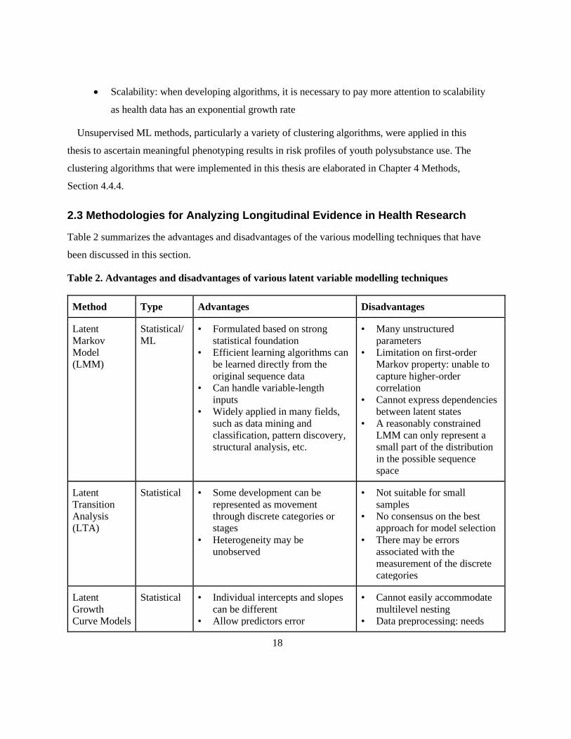
18
• Scalability: when developing algorithms, it is necessary to pay more attention to scalability
as health data has an exponential growth rate
Unsupervised ML methods, particularly a variety of clustering algorithms, were applied in this
thesis to ascertain meaningful phenotyping results in risk profiles of youth polysubstance use. The
clustering algorithms that were implemented in this thesis are elaborated in Chapter 4 Methods,
Section 4.4.4.
2.3 Methodologies for Analyzing Longitudinal Evidence in Health Research
Table 2 summarizes the advantages and disadvantages of the various modelling techniques that have
been discussed in this section.
Table 2. Advantages and disadvantages of various latent variable modelling techniques
Method Type Advantages Disadvantages
Latent
Markov
Model
(LMM)
Statistical/
ML
• Formulated based on strong
statistical foundation
• Efficient learning algorithms can
be learned directly from the
original sequence data
• Can handle variable-length
inputs
• Widely applied in many fields,
such as data mining and
classification, pattern discovery,
structural analysis, etc.
• Many unstructured
parameters
• Limitation on first-order
Markov property: unable to
capture higher-order
correlation
• Cannot express dependencies
between latent states
• A reasonably constrained
LMM can only represent a
small part of the distribution
in the possible sequence
space
Latent
Transition
Analysis
(LTA)
Statistical • Some development can be
represented as movement
through discrete categories or
stages
• Heterogeneity may be
unobserved
• Not suitable for small
samples
• No consensus on the best
approach for model selection
• There may be errors
associated with the
measurement of the discrete
categories
Latent
Growth
Curve Models
Statistical • Individual intercepts and slopes
can be different
• Allow predictors error
• Cannot easily accommodate
multilevel nesting
• Data preprocessing: needs
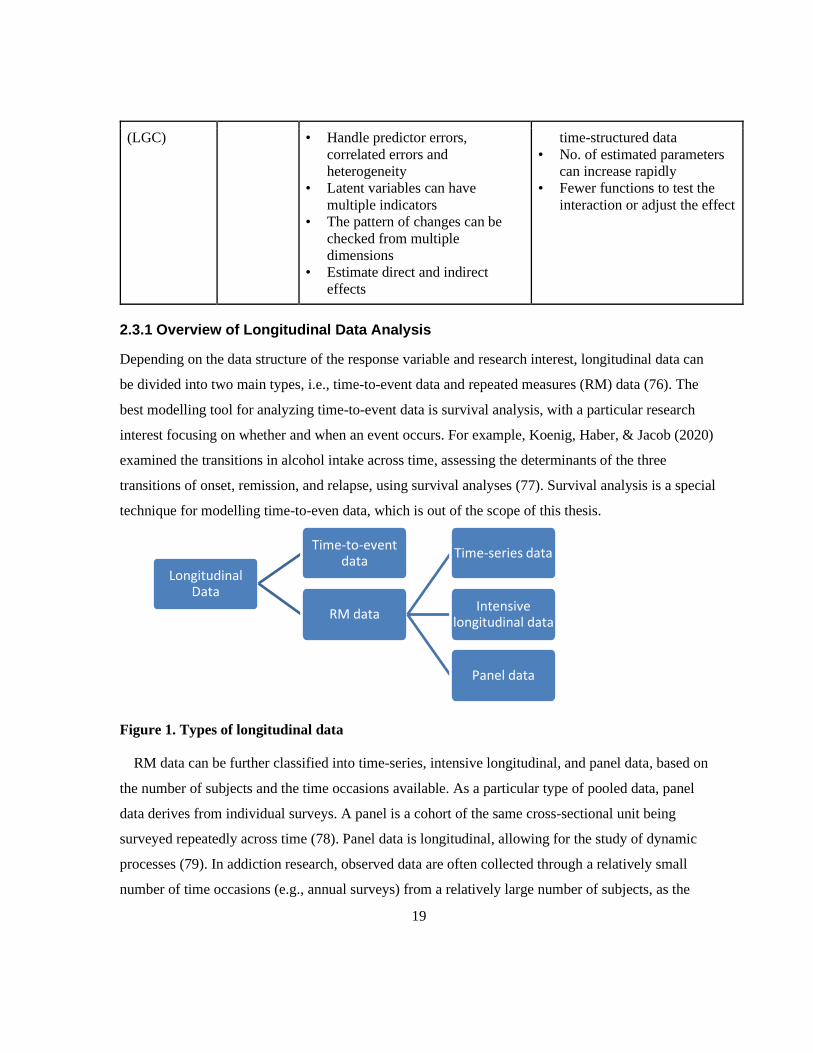
19
(LGC) • Handle predictor errors,
correlated errors and
heterogeneity
• Latent variables can have
multiple indicators
• The pattern of changes can be
checked from multiple
dimensions
• Estimate direct and indirect
effects
time-structured data
• No. of estimated parameters
can increase rapidly
• Fewer functions to test the
interaction or adjust the effect
2.3.1 Overview of Longitudinal Data Analysis
Depending on the data structure of the response variable and research interest, longitudinal data can
be divided into two main types, i.e., time-to-event data and repeated measures (RM) data (76). The
best modelling tool for analyzing time-to-event data is survival analysis, with a particular research
interest focusing on whether and when an event occurs. For example, Koenig, Haber, & Jacob (2020)
examined the transitions in alcohol intake across time, assessing the determinants of the three
transitions of onset, remission, and relapse, using survival analyses (77). Survival analysis is a special
technique for modelling time-to-even data, which is out of the scope of this thesis.
Figure 1. Types of longitudinal data
RM data can be further classified into time-series, intensive longitudinal, and panel data, based on
the number of subjects and the time occasions available. As a particular type of pooled data, panel
data derives from individual surveys. A panel is a cohort of the same cross-sectional unit being
surveyed repeatedly across time (78). Panel data is longitudinal, allowing for the study of dynamic
processes (79). In addiction research, observed data are often collected through a relatively small
number of time occasions (e.g., annual surveys) from a relatively large number of subjects, as the
Longitudinal Data
Time-to-event data
RM data
Time-series data
Intensive longitudinal data
Panel data
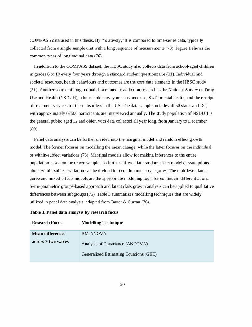
20
COMPASS data used in this thesis. By “relatively,” it is compared to time-series data, typically
collected from a single sample unit with a long sequence of measurements (78). Figure 1 shows the
common types of longitudinal data (76).
In addition to the COMPASS dataset, the HBSC study also collects data from school-aged children
in grades 6 to 10 every four years through a standard student questionnaire (31). Individual and
societal resources, health behaviours and outcomes are the core data elements in the HBSC study
(31). Another source of longitudinal data related to addiction research is the National Survey on Drug
Use and Health (NSDUH), a household survey on substance use, SUD, mental health, and the receipt
of treatment services for these disorders in the US. The data sample includes all 50 states and DC,
with approximately 67500 participants are interviewed annually. The study population of NSDUH is
the general public aged 12 and older, with data collected all year long, from January to December
(80).
Panel data analysis can be further divided into the marginal model and random effect growth
model. The former focuses on modelling the mean change, while the latter focuses on the individual
or within-subject variations (76). Marginal models allow for making inferences to the entire
population based on the drawn sample. To further differentiate random effect models, assumptions
about within-subject variation can be divided into continuums or categories. The multilevel, latent
curve and mixed-effects models are the appropriate modelling tools for continuum differentiations.
Semi-parametric groups-based approach and latent class growth analysis can be applied to qualitative
differences between subgroups (76). Table 3 summarizes modelling techniques that are widely
utilized in panel data analysis, adopted from Bauer & Curran (76).
Table 3. Panel data analysis by research focus
Research Focus Modelling Technique
Mean differences
across ≥ two waves
RM-ANOVA
Analysis of Covariance (ANCOVA)
Generalized Estimating Equations (GEE)

21
Within-subject
variation across ≥
three waves
Quantitative variations: multilevel model, latent curve model, mixed-
effects model
Qualitative variations: general growth mixture model
Qualitative + Quantitative variations: semiparametric group-based
approach, latent class growth analysis
Change in one process
related to another
Trajectories: multivariate growth model
Pairs of time points: latent change score model
Bidirectional effects
over time
Auto-regressive (AR) cross lag
Change + bidirectional Latent curve model with structured residuals
Progression through
stages/sequence
Latent transition analysis (LTA)
2.3.2 Statistical Methods
LTA, a longitudinal extension to LCA, analyzes longitudinal data to determine a transition between
latent classes across time. Suppose a change occurs, how that transition is characterized (68). In LTA,
latent classes are called latent states to convey the potentially temporary nature of the grouping (68).
In addiction research, LTA is a commonly used analytic technique that helps researchers identify
hidden subgroups of individuals within a population. In LCA, the classes (latent states) are static, but
in LTA, the classes are dynamic, such that individuals can transition from one class to another across
time. In LTA, researchers are interested in understanding how subjects transition over time between
subgroups that are identified using LCA. Different individuals may take different pathways over time,
which is what researchers are primarily interested in examining.
For example, given that social networks are complex and multidimensional, Bray and colleagues
used LTA to understand why smokers become more socially isolated when they try to quit. In this
work, LTA was first used to describe subgroups of individuals post-quit with different social
networks and then examine the dynamic transition of social network types over time (81). The study
used data from the Wisconsin Smokers' Health Study, a long-term smoking cessation trial in
Wisconsin (81). This analysis looked at 691 smokers who completed assessments at baseline and then

22
at one, two, and three years post-quit (81). The research focused on transitions of former smokers'
social network statuses across that three-year post-quit date. In addition to understanding how people
transition, the authors also examined how these different transitions were associated with abstinence
over time. Modelling multiple features of social networks simultaneously allows researchers to
explore how various sources of smoking exposure work together holistically (81). The authors also
linked transitions of class membership to other outcomes. This study underscores the need for
interventions that address situations in which subjects had partners who smoke and suggest new
interventions to target broader social networks as people attempt to quit smoking (81).
2.3.3 A Brief Introduction to Transition Models
Transition models are statistical methods used to analyze longitudinal data to study change across
time with natural, historical data. Transition models focus on modelling the response variable 𝑦𝑖𝑡 for
subject 𝑖 at time occasion 𝑡, conditional on the subject's history, denoted as 𝐻𝑖𝑡,
𝐻𝑖𝑡 = {𝑦𝑖𝑘 , 𝑘 = 1,2, … , 𝑡 − 1} (1)
Such methods are often modelled as a 𝑛-order Markov chain, where the conditional distribution of 𝑦𝑖𝑡
depends only on the most previous 𝑛 responses for subject 𝑖,{𝑦𝑖𝑡−1, 𝑦𝑖𝑡−2, … , 𝑦𝑖𝑡−𝑛}. A Markov
process is a chain of memoryless events, assuming that the next event will depend only on what is
happening now and not what happened previously.
The LMM is a generative model for analyzing panel data (82). As one practical class of
probabilistic template models, the LMM contains two probabilistic components, the transition model
and the observation model. The former reveals the change from one hidden state to another across
time, and the latter indicates how likely different observations can be seen in a given state.
Interestingly, the LMMs often have an internal structure that manifests most notably in the transition
model but sometimes in the observation model. Although LMMs can be viewed as a subclass of
dynamic Bayesian networks, they have a unique structure that makes them particularly useful for
many successful applications. The architecture of LMMs is very similar to that of hidden Markov
models (HMM), assuming to follow a Markov chain, typically of first order (27). Both HMM and
LMM approaches rely on a latent process with conditionally independent response variables (27).
HMMs are well-known for time-series and stochastic processes with various applications such as
robot localization, speech recognition, activity recognition, machine translation, time series
prediction, biological sequence analysis, and others (83–85). The HMMs and LMMs rely on a solid

23
statistical foundation. However, the literature also refers to such probability template models as ML
models. Therefore, the LMM lies at the intersection between statistical modelling and ML modelling.
To emphasize the analysis of longitudinal data, the LMM is the term used throughout this thesis.
2.3.4 Latent Markov Models (LMM)
The LMM was initially developed in multiple directions with applications in sociology, psychology,
and medicine (86). The first development involves using covariates, which may be included either in
the latent or measurement model. A multivariate LMM was developed by Bartolucci and Farcomeni
(2009), in which the conditional response probabilities of a given latent process were parameterized
by multivariate logistic transformation. Using both time-invariant and time-varying covariates,
Vermunt et al. (1999) modelled the initial probability and transition probability of the LMM process
with multinomial logit regression models. Further extending this method, Bartolucci et al. (2007)
applied more than one response variable, estimating transition probabilities based on lagging response
variables (87). The LMM methodology allows various models to be estimated, and the best model can
be selected from a latent class model to a heterogeneous model with subgroups.
The two fundamental problems that an LMM can address are predicting the probability of a
sequence and predicting the most likely order of latent states based on observed data. Bartolucci,
Farcomeni, & Pennoni (2012) stated two main applications of LMM, decoding and forecasting.
Decoding uses the observed data of a sample unit to predict the order of its latent states (27).
Decoding is further classified into local decoding and global decoding. The former refers to
identifying the most likely latent state for each time occasion, while the latter identifies the most
likely order of latent states. Another application of LMM is to forecast a latent state for future time
occasions or a future response, given the observed historical data (27).
LMMs have been utilized in recently published health-related research. Some examples include
examining the tendency of substance use (88), evaluating the performance of different nursing homes
(89), assessing the dynamic association between expenditures and health conditions in the ageing
population (90), and modelling the determinants of health care utilization (91). To examine whether
age is associated with an increasing tendency of marijuana consumption, Bartolucci (2006) applied a
univariate LMM (with no covariates) to the “National Youth Survey” data with five annual waves of
marijuana consumption. The analysis was based on three latent states (not inclined to use cannabis,
incidental use of cannabis, and inclined to use cannabis), with homogenous transition probabilities

24
and a parametric measurement model with simplicity provided global logits. The author tested
different hypotheses of the latent process on the transition matrix. A tridiagonal structure was
identified for the transition matrix. It has been proven that the LMM can handle distribution
assumptions, such as excessive dispersion of polynomial distribution flexibly, considering the
measurement error (88).
Mitchell et al. (2008) examined the drinking patterns of American Indian adolescents, the
predictive factors and developmental outcomes that co-occurred (92). The authors applied an LMM to
6 bi-annual data collected from American Indian high school students to study dynamics in latent
statuses of youth alcohol drinking in the past six months (92). The three latent statuses identified to
describe alcohol drinking patterns across the three years were: abstainers, inconsistent drinkers, and
consistent drinkers (92). The modelling results provide valuable insights into distinguishing youth
who should be considered inconsistent drinkers (92). This study also indicates that extensive
interventions for youth may not be the most important measures to minimize adverse health
outcomes. Given limited resources, future interventions for alcohol intake and the use of other drugs
may be more strategic (92).
The dynamic LMM has also been used to model the determinants of health care utilization leading
to policy implications. Gil, Donni, & Zucchelli (2019) applied a bivariate LMM to model healthcare
usage trends, dynamic unobserved heterogeneity, transitions between latent states, and the
endogeneity of uncontrolled diabetes (91). The authors estimated the impact of uncontrolled diabetes
on primary and secondary health care use on longitudinal administrative data, using biomarkers to
measure uncontrolled diabetes (91). An LMM was applied to the longitudinal health survey and
registration data on health care expenditures to examine the dynamic association between
expenditures and health status in the ageing population (90).
Rijmen, Vansteelandt, & De Boeck proposed a hierarchical structure of the LMM to examine the
emotional change process of patients with anorexia based on the ecological transient assessment
research (93). Four latent states were selected for the analysis, including “positive mood,” “neutral to
moderately positive mood,” “low intensity for all emotions except tension,” and “negative mood”
(93). To illustrate that data from different day levels are dependent, Rijmen et al. (2008) fitted a
hierarchical LMM by incorporating latent variables at the day level. Assuming a first-order Markov
chain that is time-homogeneous, the author modelled the dynamics between the latent statuses at
25
signal- and day levels. It is estimated that there will be more positive sentiment trends in the initial
probability and conditional probability of the chain over signal and day (93).
Bartolucci, Lupparelli, & Montanari proposed an LMM for assessing the performance of different
nursing homes regarding the level of care provided for their patients in one region of Italy (89). This
study is about the evolution of psycho-physic conditions of a sample of elderly individuals hosted in
certain Italian nursing homes. Assuming a latent Markov chain exists for the transition of patients'
health conditions, the LMM is used to analyze the repeated administration of questionnaires. With a
manageable number of nursing homes (11) in this study, the authors utilized the multilevel structure
of this longitudinal dataset. Instead of using random effects, fixed effects were applied to capture the
impact of each institution on their patients' health conditions. The advantage of this method is that it
explicitly considers the transition of health conditions, which is the metric used to evaluate the
nursing homes' performance. However, this application may need a multilevel approach based on
random effects with many clusters.
The LMM approach has also been applied in psychological and educational research (94), labour
market and marketing-related fields (95), criminological research (87), and many others.
2.3.5 Multilevel Model (MLM) Framework
The MLM framework is a hierarchical modelling approach that allows for nested data structure and
provides clear and structured semantic descriptions of growth pathways. There are other terms in the
literature, such as hierarchical linear model, general linear mixed model, GCM, and random
coefficient model (96,97). Although these models are not identical, their analytic approach is similar.
They contain variables defined at different levels of the structured population with hierarchy; thus,
these terms can be used interchangeably in practice.
LMMs can be extended to multilevel data, where individual samples are collected into subgroups.
The fact that the samples are hierarchical is sufficient. Significant intraclass correlation coefficients
(ICC) between levels are not required. Based on fixed effects, Bartolucci et al. (2009) employed a
method to represent the common factors of all samples in the same subgroup. Based on random
parameters with discrete distribution, Bartolucci et al. (2011) proposed a method related to mixed
LMMs and LMM with random effects. These formulations for multilevel data are related to the
extended LMM, allowing parameters to be changed in different latent subgroups. This method is
known as the foundation of LTA (98).

26
This particular modelling technique has been applied in healthcare services, such as assessing the
nursing homes' performances (99) and school services. For example, Bartolucci and colleagues (100)
evaluated school performance, and Williford and Zinn identified bullying experiences with
classroom-level mixtures taking advantage of nested structures of peer children in the classroom and
school environments (101). These studies provide insights into individualized interventions
corresponding to different latent states and transitions. This multilevel approach allows us to fit and
further extend the LMMs by applying that same concept but at the level of repeated measures.
Koukounari et al. (2013) used a nonparametric multilevel LMM approach to study two trachoma-
endemic communities in Gambia and Tanzania (102). This approach allows for nested data structure
and addresses the computational difficulties of the multilevel longitudinal mixed model.
Simultaneously, this study assesses three diagnostic and variance tests without a gold standard, based
on data collected from a large-scale drug management intervention (102). The Multilevel LMM was
used to assess the impact of interventions on infection and disease prevalence. Level 1 and level 2
were the within-household model and the between-household model, respectively.
2.4 ML in Public Health
The two most common public health topics where ML is currently employed are chronic diseases and
associated risk factors and infectious, parasitic, and communicable diseases (20). The most common
ML algorithms used in the literature were classification algorithms, including decision trees, random
forest, logistic regression, and support vector machines (20). It is likely driven by the number of use
cases where text mining and sentiment analysis were used to classify the concerns of individuals
towards public health problems. This analysis was most commonly completed using free/open-source
tools like R and Python. Common datasets that were used for this analysis included census data,
social media data (e.g., Twitter), and specialized databases such as vaccine or risk databases (20).
Most ML techniques have been applied for descriptive and predictive purposes by mapping inputs
to outputs in a data-driven manner. The objective includes public health surveillance, disease
diagnosis, disease incidence, and individual-level and population-level prediction (19). ML offers
health researchers new tools to tackle problems for which classical statistical methods may encounter
limitations. ML is well-equipped to analyze vast amounts of health, environmental and other geo-
special data to explore associations, identify disease patterns, and predict health outcomes in a

27
population, when it occurs, how it changes, and predict the impact of interventions or solutions (18).
ML techniques may also generate hypotheses from large datasets and could be used to inform health
research (19). ML can help public health researchers explore causality in some studies, although these
methods do not necessarily change our conceptual understanding of the causal paradigm (17).
ML provides tremendous opportunities for improving public health. In a presentation of ML for
public health hosted by Public Health Ontario, Rosella, Fisher, and Song (2019) summarized the
rationale behind the rapidly growing interest in AI, including quickly evolving data environment,
increasing computational capacity, improvements in data ingestion and processing, and greater
demand for data-driven decisions (17). All these elements nurture our developing data science
ecosystem in the public health sector. Population health focuses on the health outcomes of a group of
people and the distribution of their results. Public health information has a considerable volume and
can be viewed as the data source for ML, paving the way for precision public health (21). This term
has recently been used in the public health literature, referring to “providing the right intervention to
the right population at the right time (103).”
In the early days of designing this thesis, we conducted some preliminary searches for the topic of
“ML for Public Health” on a variety of bibliographic databases, including PubMed, Scopus, IEEE,
Web of Science, ACM, and ProQuest. From this preliminary search, ML applications in public health
are primarily focused on infectious disease epidemics, lifestyle diseases, and predicting demographic
information. Major themes have emerged in the field of public health through the application of ML
methods, including disease screening/prediction/detection/outbreak/surveillance, non-communicable
diseases, communicable/infectious diseases, risk factors/behaviours, mental health, maternal and child
health, accidents/injuries/disability, and respiratory diseases and allergic disorders (104).
Some key enablers to facilitate the use of ML to understand and tackle public and population health
problems have been identified (105). These enablers include understanding the governance context of
big data in public health, modernizing data and analytic infrastructure, applying ML best practices,
nurturing educated staffing, and establishing strategic collaborative partnerships between ML
researchers and public health professionals. The significant hurdles of ML in public health include
data acquisition (access and sharing), informed consent, security and privacy concerns, and making
decisions under uncertainty (16,19). Overfitting is also a concern, which requires careful model
evaluation before deployment. The potential ethics and bias-related issues related to ML-based

28
systems must also be considered. For example, biased data can lead to faulty algorithms, intensifying
public health issues at the community level. How do we ensure that the data we are training and
validating these automation tools do not contain inherent bias? Ethical issues such as who is
accountable in the event of an error. Security and privacy of patient health data will be an ongoing
concern (106). Achieving fairness, accountability and transparency (FAT) is the goal of explainable
ML in the public health sector, with an interdisciplinary research focus. However, it is at an early
stage of adopting ML in public health, and the level of sophistication is deficient.
In summary, this chapter provided a literature review on youth polysubstance use, approaches for
modelling cross-sectional data in addiction research, advanced methods in transition modelling, and
ML in public health. The review explained the methodologies utilized, their applications, and
comparisons drawn by diverse research in the published literature. The research gap was identified
that ML approaches had not been widely applied in addiction research. The study rationale and
specific objectives follow in the next chapter.
29
Chapter 3
Study Rationale and Objectives
This chapter presents the rationale for this study and summarizes the aims, specific objectives, and
research questions for this thesis.
3.1 Study Rationale
Although it is known that healthy habits during adolescence tend to persist into adulthood, the amount
of research focusing on social correlates of youth health behaviours (e.g., peer relations, parental
support, school programs) has been inadequate (107). The COMPASS longitudinal study addresses
this gap by collecting multifaceted information pertaining to youth health behaviours from multiple
sources to examine the relationship between school environmental characteristics and youth health
behaviours in Canada. The COMPASS dataset is diverse, including Cq, BE assessments and policy
evaluations. It has been utilized in many health-related disciplines. The COMPASS research has
produced over a hundred academic publications ranging from environmental health and health
promotion to preventative medicine (108). Early COMPASS publications revealed the substantial
variability across Canadian jurisdictions regarding youth PA levels, substance use, mental well-being,
and healthy school environments and policies (59). The COMPASS data have been continuously used
to assess how school environments, policies, and practices affect multiple youth health behaviours
and outcomes (59).
From a methodological perspective, the existing literature using the COMPASS data primarily
applied LCA or LPA to identify single substance use patterns. For example, Lee et al. (2021)
examined stage-sequential alcohol drinking patterns using multilevel latent class profile analysis
(109). Gohari et al. (2020) applied a multilevel LCA to discover alcohol consumption patterns
among youths from Canadian secondary schools (65). Hammami et al. (2019) studied risk behaviours
associated with BMI on chronic diseases using the sex-stratified multilevel LCA approach (110). In
addition, using LCA, Laxer et al. (2017) examined modifiable behaviours and their impact on obesity
and overweight among adolescents (111).
However, none of the studies that used COMPASS data examined the transition of polysubstance
use patterns among youth across time or explored risk profiling based on student characteristics and

30
school environment perspectives. Furthermore, current studies using the COMPASS data
predominately select features for modelling based on a priori knowledge from existing literature in
the appropriate research domain. By discriminatingly selecting only a few variables from the dataset
that the researchers deem relevant to their study, they may inadvertently overlook meaningful
relationships, hidden patterns, or underlying trends that could have been captured with the omitted
variables. This could result in missed opportunities in identifying critical information to revise
policies and interventions concerning youth health behaviours in school settings. Additionally,
selectively overlooking variables provides an opportunity for implicit biases that can then be further
imparted into the data analysis.
ML algorithms have unique advantages for revealing “hidden” patterns and unexpected
associations in large and complex datasets, discovering relevant patterns in such high-dimensional
data that are structural and/or temporal. Unless otherwise well-established, these patterns
(“knowledge”) are often unobservable, and human experts cannot directly access them. Yet, we may
need these patterns to assist in better decision support. Most population-level health data are non-
standardized and are often weakly structured, with a high dimension >3 (112). Although human
experts are good at ≤3-dimensional pattern recognition, any higher-dimensional datasets make
manual analysis difficult and impossible (112). We are unsure about the hidden knowledge, and ML
approaches hold a promise to quickly identify hidden patterns on a vast volume of health data.
However, thus far, none of the published studies using the COMPASS data have applied ML
methods. This thesis employed ML techniques to the COMPASS dataset to enhance data exploration
capabilities and identify complex associations between variables. On the one hand, the COMPASS
dataset is explicitly concerned with youth health behaviours and corresponding school policies and
practices. On the other hand, the multifaceted characteristics of this large-scale survey data, including
the complexity of influence/behaviour models, modifiable risk factors, and disease progression and
intervention, make it the optimal candidate for ML approaches in population-based health research.
3.2 Objectives
ML in public health is a new field, and its applications are underutilized. This thesis is designed to
realize the huge potential of ML applications in the public health domain, engaging ML practitioners
to move towards research in this field and bridging these two communities. The overarching goal of
this thesis is to further the understanding of the appropriate way of fitting transition models and

31
exploring the “hidden” patterns generated from large complex population-based health survey data.
The research objectives are achieved by implementing appropriate ML models to the COMPASS
data.
First, this thesis aims to apply an LMM technique on longitudinal data to explore the dynamic
transitions of polysubstance use patterns from one state to another across time, showcasing the ability
of this type of modelling technique to examine inter-individual differences in transition analysis.
Second, unsupervised ML algorithms have the unique advantages of revealing “hidden” patterns and
unexpected associations in a large and complex dataset. The secondary aim of this thesis is to explore
and obtain a better understanding of the structure of the COMPASS data in the context of risk
profiling of polysubstance use among youth, which is primarily achieved through the application of
cluster analysis.
More specifically, the objectives of this thesis are to:
• Estimate the transition probabilities of dynamic membership of use patterns over time using
the COMPASS data.
• Experiment and apply a variety of clustering algorithms to analyze the COMPASS data that
are explainable.
• Identify the most significant features or actionable insights for polysubstance use prevention
derived from an ML model.
3.3 Research Questions
This thesis investigates how the various ML models can be applied to the longitudinal data for
analyzing polysubstance use among adolescents using the COMPASS dataset. According to the
literature on youth polysubstance use, it is anticipated to identify several latent states (subgroups) of
individuals differing in their use patterns and transition over time. More specifically, this thesis is set
to address the deficiency in understanding the dynamic transitions of use patterns using the
COMPASS data.
3.3.1 Primary Research Questions
The primary research questions are:

32
• RQ1: What are the risk profiles of polysubstance use among Canadian secondary school
students?
• RQ2: What are the patterns of polysubstance use among Canadian secondary school
students?
• RQ3: How do transition behaviours change over time in use patterns?
3.3.2 Secondary Research Questions
The secondary research questions include:
• RQ4: What factors are associated with patterns of polysubstance use among Canadian
adolescents?
• RQ5: What factors are associated with dynamic transitions of use patterns?
• RQ6: What are the advantages and limitations of the ML methods appropriate to modelling
risk profiles and dynamic transitions using the COMPASS data?
In summary, this chapter provided the study rationale and summarized the specific objectives and
research questions for this thesis. The research methodologies throughout this thesis follow in the
next chapter.
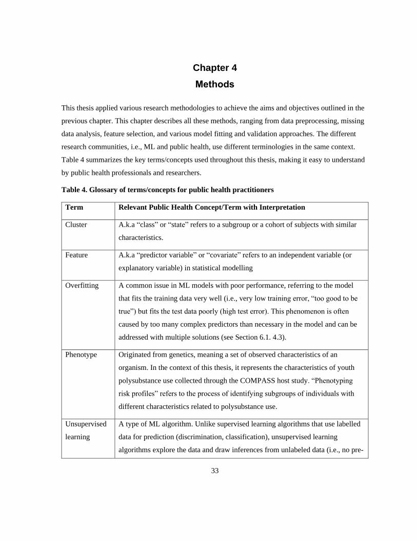
33
Chapter 4
Methods
This thesis applied various research methodologies to achieve the aims and objectives outlined in the
previous chapter. This chapter describes all these methods, ranging from data preprocessing, missing
data analysis, feature selection, and various model fitting and validation approaches. The different
research communities, i.e., ML and public health, use different terminologies in the same context.
Table 4 summarizes the key terms/concepts used throughout this thesis, making it easy to understand
by public health professionals and researchers.
Table 4. Glossary of terms/concepts for public health practitioners
Term Relevant Public Health Concept/Term with Interpretation
Cluster A.k.a “class” or “state” refers to a subgroup or a cohort of subjects with similar
characteristics.
Feature A.k.a “predictor variable” or “covariate” refers to an independent variable (or
explanatory variable) in statistical modelling
Overfitting A common issue in ML models with poor performance, referring to the model
that fits the training data very well (i.e., very low training error, “too good to be
true”) but fits the test data poorly (high test error). This phenomenon is often
caused by too many complex predictors than necessary in the model and can be
addressed with multiple solutions (see Section 6.1. 4.3).
Phenotype Originated from genetics, meaning a set of observed characteristics of an
organism. In the context of this thesis, it represents the characteristics of youth
polysubstance use collected through the COMPASS host study. “Phenotyping
risk profiles” refers to the process of identifying subgroups of individuals with
different characteristics related to polysubstance use.
Unsupervised
learning
A type of ML algorithm. Unlike supervised learning algorithms that use labelled
data for prediction (discrimination, classification), unsupervised learning
algorithms explore the data and draw inferences from unlabeled data (i.e., no pre-
34
defined outcome variable) to uncover inherent structure or hidden patterns. As
one type of unsupervised learning, cluster analysis has been extensively
investigated and applied to partition data into homogenous clusters (see Section
2.2.2.2).
4.1 Study Design and Participants
This study is a retrospective cohort study, taking the secondary analysis approach of an ongoing
longitudinal study, i.e., the COMPASS study. The COMPASS data are a de-identified health survey
at the population level. As introduced in Section 2.1.4.1, the COMPASS study collects student- and
school-level information from a convenience sample of secondary schools across several provinces in
Canada each school year (59,60). Substantial efforts have also been made to streamline data
collection methods to minimize interruptions to class time and reduce the burden of work on
participating schools (113). Eligible students at participating secondary institutions complete the
questionnaire during class time on a prearranged “data collection day” (114).
Since COMPASS research involves youth under 18 years old, parental/guardian consent is required
for participation. The University of Waterloo Office of Research Ethics has approved the active-
information passive-consent protocols, which help achieve high participation rates and reduce
sampling bias while preserving student confidentiality (113). The protocol provides parents with
pamphlets that detail important COMPASS research and contact information, including contact
information of the recruitment coordinator if parents would like to withdraw their child(ren) from the
study. Eligible students whose parents do not contact the recruitment coordinator within the two-week
time frame provided are considered participants who are allowed to complete the Cq (113).
Additionally, students are permitted to withdraw participation during the consent process or data
collection period (59).
In this thesis, the three-year linked sample of the COMPASS data collected includes Wave I (the
school year 2016-2017, Y5), Wave II (the school year 2017-2018, Y6), and Wave III (the school year
2018-2019, Y7). The COMPASS study has received ethics clearance from the University of Waterloo
Office of Research Ethics (ORE 30118).
35
4.2 Dataset and Data Preprocessing
4.2.1 Dataset
The longitudinal dataset being analyzed in this study is the three-year linked sample of the
COMPASS data collected from Wave I, Wave II, and Wave III. Each linked dataset contains over
200 variables collected from 9307 Canadian students from grades 7 to 12 (secondary I through V in
Quebec) at the initial measurement occasion (Wave I). The participating students were from 76
secondary schools located in Ontario, Quebec, British Columbia, and Alberta. Of the 9307 linked
samples, the present analyses are restricted to the 8824 students with regular patterns on their grade
levels. “Regular patterns” refer to the advancement of students from one grade to another at each
school year. The COMPASS host study uses grade to be relevant to school planners who make plans
based on grade, not age. Thus, the students’ grade level is a proxy of their age throughout this thesis.
The Cq data contains demographic and personal information, such as grade, sex, ethnicity, primary
language spoken, height and weight. Additionally, it includes student responses to multiple-choice
questions regarding their behaviour and perspectives on health and wellness topics. The
supplementary community-level data, i.e., school-level socioeconomic status, urbanity, and BE, are
linked to each participating school. The survey is conducted annually, with three consecutive waves
available for each subject within the same cohort.
As previously discussed, the COMPASS data is collected using annual student questionnaires Cq,
school program/policy questionnaires (SPP, completed by a school administrator), and
internal/external school environmental assessments (Co-SEA) (59). Students complete the cover page
of the Cq to generate a unique code that allows COMPASS researchers to link data collected from the
same student across multiple years of participation (59). The use of self-generated identification
codes for anonymizing questionnaire data collected in longitudinal studies has been well documented
and strikes a favourable balance between privacy and research methodology (115). Anonymization
using unique self-generated codes is perhaps the principal strategy for ensuring COMPASS data
remains confidential throughout the remainder of its life cycle.
Although the SPP data provides a wealth of information regarding policies and programs, they are
not commonly used as student-level data, possibly due to the qualitative nature of many open-ended
text responses. Since the research focus of this thesis is not directly related to the content from SPP
36
data, it was excluded in this thesis. Of note, the initial three waves COMPASS data contains 46862,
66434, and 74501 subjects at Y5, Y6, and Y7, respectively. To distinguish the initial three waves data
and the linked samples, Wave I, Wave II, and Wave III are used throughout this thesis, representing
linked samples at Y5, Y6, and Y7, respectively.
4.2.2 Data Preprocessing
Several data preprocessing steps were taken to prepare the data for analyses, including data cleaning,
linking, merging, and missing data analysis. Figure 2 illustrates the flowchart of the steps taken from
full samples down to final linked samples.
Figure 2. Flowchart of data preprocessing
4.2.2.1 Step 1: Data Cleaning
Redundant variables, such as nested questions which tend to have redundant information, and
irrelevant variables, such as information inconsequential for analyses, were removed. For example,
the subsequent question, “In the last 12 months, how often did you use marijuana or cannabis? (a
joint, pot, weed, hash)” is, “If you have used marijuana or cannabis in the last 12 months, how did
you use it?” Since the response to the nested question assumes an affirmative response to the parent
question, such questions were considered redundant and thus were removed from the analyses.
Redundant and irrelevant variables were identified by individually reviewing each nested question.
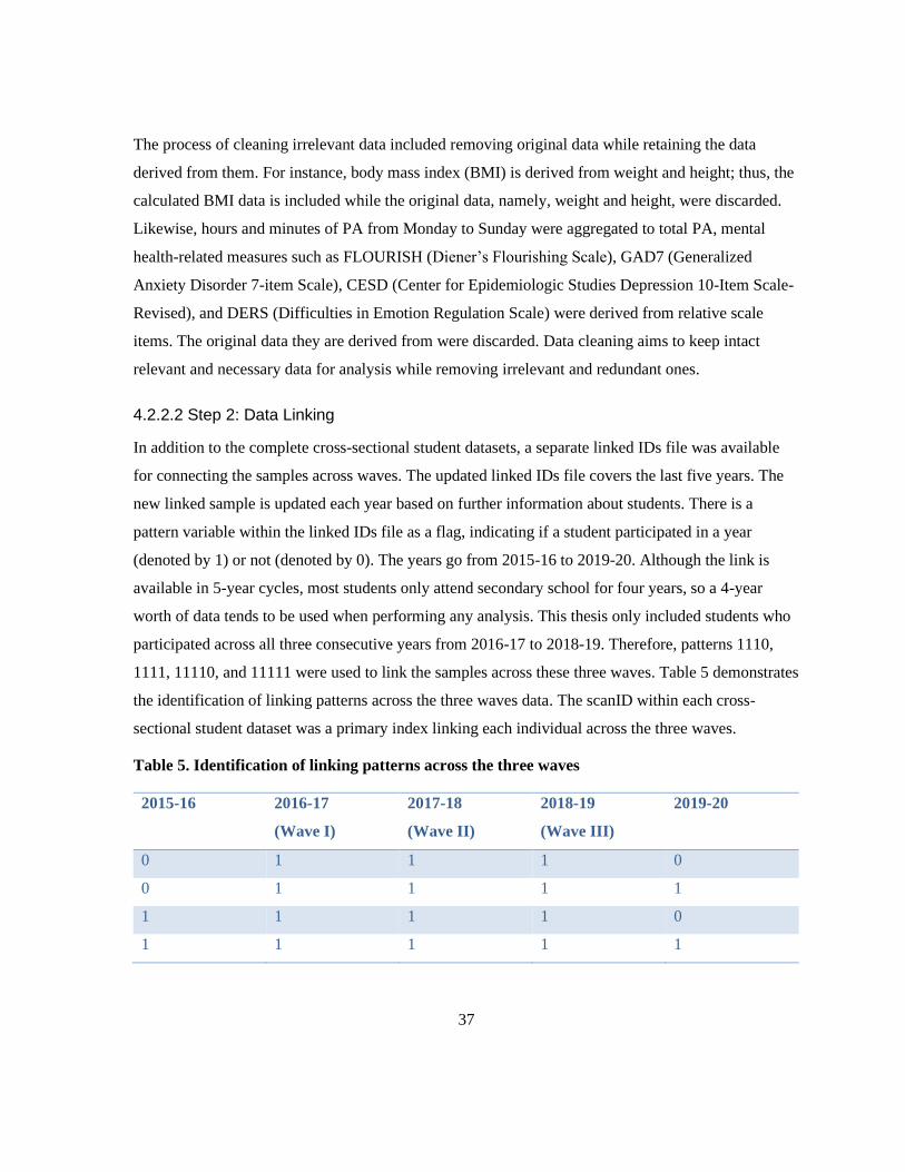
37
The process of cleaning irrelevant data included removing original data while retaining the data
derived from them. For instance, body mass index (BMI) is derived from weight and height; thus, the
calculated BMI data is included while the original data, namely, weight and height, were discarded.
Likewise, hours and minutes of PA from Monday to Sunday were aggregated to total PA, mental
health-related measures such as FLOURISH (Diener’s Flourishing Scale), GAD7 (Generalized
Anxiety Disorder 7-item Scale), CESD (Center for Epidemiologic Studies Depression 10-Item Scale-
Revised), and DERS (Difficulties in Emotion Regulation Scale) were derived from relative scale
items. The original data they are derived from were discarded. Data cleaning aims to keep intact
relevant and necessary data for analysis while removing irrelevant and redundant ones.
4.2.2.2 Step 2: Data Linking
In addition to the complete cross-sectional student datasets, a separate linked IDs file was available
for connecting the samples across waves. The updated linked IDs file covers the last five years. The
new linked sample is updated each year based on further information about students. There is a
pattern variable within the linked IDs file as a flag, indicating if a student participated in a year
(denoted by 1) or not (denoted by 0). The years go from 2015-16 to 2019-20. Although the link is
available in 5-year cycles, most students only attend secondary school for four years, so a 4-year
worth of data tends to be used when performing any analysis. This thesis only included students who
participated across all three consecutive years from 2016-17 to 2018-19. Therefore, patterns 1110,
1111, 11110, and 11111 were used to link the samples across these three waves. Table 5 demonstrates
the identification of linking patterns across the three waves data. The scanID within each cross-
sectional student dataset was a primary index linking each individual across the three waves.
Table 5. Identification of linking patterns across the three waves
2015-16 2016-17
(Wave I)
2017-18
(Wave II)
2018-19
(Wave III)
2019-20
0 1 1 1 0
0 1 1 1 1
1 1 1 1 0
1 1 1 1 1
38
4.2.2.3 Step 3: Data Merging
The supplementary school-level data, including household income level and urbanity, were merged
into the student-level dataset using the corresponding school ID as the primary index. For the school-
level BE, although 1500 meters is closer to the 1-mile buffer often used in US studies (116), the
radial distance for points of interest, such as drug and liquor stores, were selected to be within1000
meters of the school zone. This distance of 1000 meters has commonly been used in tobacco retailer
density literature for examining the relationship between school environments and youth smoking
behaviours since it is relatively close to the school (117,118). The radial distance of 1000 meters
approximates the furthest commuting distance for students from home to school, approximately 15-20
minutes walking distance. The school-level BE variables that were utilized in this thesis include total
points of interest, such as the number of locations that sell alcohol, drugs, and tobacco products,
within a 1000 meters radius of a school.
4.2.2.4 Step 4: Missing Data Analysis
Missing data were analyzed by identifying the missing patterns. Multiple imputations (MI) for
missing values were performed by implementing the MICE (Multivariate Imputation via Chained
Equations) package, generating five imputed datasets, with 50 iterations for each imputed dataset. It is
assumed that the missing values are Missing at Random (MAR) using the MICE package. Missing
data were imputed by specifying an imputation model for each variable with missing values one by
one. For numeric variables, such as total points of interest within the school BE, sedentary time in
minutes, total scores related to mental health assessment like CESD, predictive mean matching
(PMM) was selected as the method for MI. A logistic regression model was specified for binary
variables, responses with only two levels/options, e.g., gamble online for money (Yes/No). In
contrast, for unordered factor variables with more than two levels, e.g., ethnicity
(“White/Black/Asian/Indigenous/Latin American/Other”), a polytomous logistic regression was
specified for imputing missing values. Lastly, for ordered factor variables with greater than two
levels, e.g., evaluating the level of school support available for students to help quit drugs and/or
alcohol (“Very supportive/Supportive/Unsupportive/Very unsupportive”), a proportional odds model
was specified. After performing MI, statistical tests on each imputed dataset were conducted to pool
the results for summary estimates. The optimal imputed dataset was identified by obtaining the best
pooling statistical tests on most covariates.
39
Of note, the mental health-related items (FLOURISH, GAD7, CESD, and DERS) and the online
gamble question were not asked in the Year 5 survey questionnaire. Those items were collected from
Year 6 onwards. Since these variables are completely missing and the missing value imputation was
not applicable for this type of missingness, these variables were imputed based on “Next Observation
Carried Backward (NOCB).” NOCB is a reverse approach to the well-known “Last Observation
Carried Forward (LOCF)” method by taking the first available value after the missingness and
moving it backward (119). In addition to these missing values, BMI has been top missingness across
the three waves data. Since BMI data are usually missing not at random (MNAR), multiple
imputations may not be appropriate for this specific variable. In some papers, what researchers have
done instead is coded missing as its category. Instead of the initial four classification categories, i.e.,
underweight, healthy weight, overweight, and obese, one more category was added, representing “not
stated.” In this thesis, we follow the same strategy of imputing the BMI missing data.
4.3 Substance Use Indicators
Substance use indicators, including cigarette smoking, e-cigarette use, alcohol drinking, and
marijuana consumption, were assessed using the COMPASS Cq. Given that there is so much
variability in the initial responses to the use frequency of the four substances (ranging from 1 to 8 or 1
to 9 for each substance), it generates a relatively large contingency table with 8 x 8 x 9 x 9 = 5184
cells. Each cell of the contingency table corresponds to the combination of response patterns of
substance use. As this thesis focuses on risk profiles and use patterns rather than frequencies, the
ordinal responses were collapsed into three-category indicators to avoid the sparseness of the
observed frequency table. Following the most common categorization for determining the patterns of
youth polysubstance use, the initial responses were categorized into “0,” “1,” and "2,” representing
“never use,” “occasional use,” and “current use,” respectively. Further information on the Cq
questions and their categorization follows.
Cq posed two questions for cigarette smoking and e-cigarette use to determine the incidence and
frequency of these substances. The questions and the categorization of the initial responses can be
seen in Figures 3-4. While for alcohol drinking and marijuana consumption, only a single measure
was used on Cq. Figures 5-6 demonstrate the questions and the categorization of the initial responses
for these two substances.

40
Figure 3. Measurement of cigarette smoking
Q1: “Have you ever tried cigarette smoking, even just a few puffs?”
0 = Nnever Use
"No" "Yes"
Q2: “On how many of the last 30 days did you smoke one or more cigarettes?”
1 = Occasional Use
"None"
2 = Current Use
"1 day," "2 to 3 days," "4 to 5 days," "6 to 10 days," "11 to 20 days," "21 to 29 days," "30 days
(every day)."

41
Figure 4. Measurement of e-cigarette use
Figure 5. Measurement of alcohol drinking
Q1: “Have you ever tried an electronic cigarette, also known as an e-cigarette?”
0 = Never Use
"No" "Yes"
Q2: “On how many of the last 30 days did you use an e-cigarette?”
1 = Occasional Use
"None"
2 = Current Use
"1 day," "2 to 3 days," "4 to 5 days," "6 to 10 days," "11 to 20 days," "21 to 29 days," "30 days (every
day)."
Alcohol Drinking
Q: "In the last 12 months, how often did you have a drink of alcohol that was more than just a sip?"
0 = Never Use
• “I have never drunk alcohol”
• "I have only had a sip of alcohol"
1 = Occasional Use
• “I did not drink alcohol in the last 12 months”
• "Less than once a month"
2 = Current Use
• "Once a month"
• "2 or 3 times a month"
• "Once a week"
• "2 or 3 times a week"
• "4 to 6 times a week"
• "Every day"

42
Figure 6. Measurement of marijuana consumption
4.4 Cluster Analysis
4.4.1 Feature Selection
Feature selection and feature extraction are the two main methods of dimensionality reduction, which
is crucial in modelling, especially when the dataset contains redundant or unnecessary variables for
model fitting. To better preserve the interpretability of ML results, the feature selection approach was
employed instead of feature extraction algorithms. Feature selection refers to selecting a subset of the
original features, whereas feature extraction constructs derived features from the initial ones to
achieve good modelling performance. In this thesis, a commonly used feature selection algorithm,
Boruta, was applied to obtain the most representative subset of features for clustering. Boruta works
as a random forest-based feature selection algorithm, an ensemble of decision trees. See Appendix E
for a detailed description of the Boruta algorithm.
The same procedure of feature selection was repeated for each wave. The most notable subset of
features was identified for the cluster analysis. For each feature, the score of variable importance was
summed up across the three waves. The total score was sorted from largest to smallest. At the
experimental stage, we selected from the top one up to all the features into modelling clusters.
Preliminary results demonstrated that the number of features around 10 led to more meaningful
clustering solutions. Since the top 8 features covered as many risk aspects as the top 10, the former
Marijuana Consumption
Q: "In the last 12 months, how often did you use marijuana or cannabis? (a joint, pot, weed, hash)."
0 = Never Use
• “I have never used marijuana”
1 = Occasional Use
• “I have used marijuana but not in the last 12 months”
• “Less than once a month"
2 = Current Use
• “Once a month”
• “2 or 3 times a month”
• “Once a week”
• “2 or 3 times a week”
• “4 to 6 times a week”
• “Every day”

43
was selected for parsimonious model fitting and a more straightforward interpretation. Including the
four substance use indicators, all the variables specified in the cluster analysis were standardized to
ensure equal weighting before clustering.
4.4.2 Data Visualization
t-Distributed Stochastic Neighbor Embedding (t-SNE) was employed in this thesis to visually present
both the local and global structure of high-dimensional COMPASS data in one map. t-SNE is a non-
linear ML algorithm used for reducing dimensionality and visualizing high-dimensional data. That is,
it takes a high-dimensional dataset and projects it onto a lower-dimensional (two-dimensional or 2D
in this thesis) space for visualization. Van der Maaten & Hinton (2008) developed the t-SNE
algorithm, which has since been well adopted by various research communities, such as genomics,
natural language processing (NLP), speech recognition, and many other fields (120). t-SNE tends to
preserve both local and global structures as much as possible simultaneously. Principal components
analysis (PCA) or multi-dimensional scaling are other dimensionality reduction methods that can
preserve the global structure while losing the local structure.
An essential step to use the t-SNE algorithm effectively is to tune hyperparameters, such as
perplexity and the number of iterations. As a smooth measure of the adequate number of neighbours,
Van der Maaten suggests setting the typical range of perplexity values between 5 and 50 to achieve a
fairly robust performance of t-SNE (120). For a larger or denser dataset, the rule of thumb is to select
a larger value of perplexity (121). Oskolkov proposed the optimal perplexity approximates √𝑁2
,
which is analytically derived from the power law, given that t-SNE is based on the minimization of
Kullback-Leibler (KL) divergence (121). In this thesis, a range of perplexity, from 5 to 100, was
experimented with. Perplexity = 100, which approximates √𝑁2
, is the optimal value for the linked
three waves COMPASS datasets. A detailed description of the t-SNE algorithm can be seen in
Appendix F.
4.4.3 Determining the Optimal Number of Clusters
One of the most challenging decisions to make in cluster analysis is determining the optimal number
of clusters. When plotting the number of clusters, the optimal number can be found by observing the
number of clusters with inflection points, peaks or declining points in the evaluation measures. Some
commonly used approaches include the elbow method, silhouette analysis, the sum of squares
44
method, the GAP statistic, the D index, the Hubert index, among many others (22). For example, both
the Hubert and D index are graphical methods. They seek the significant peak that corresponds to a
substantial increase in the value of the measure. The silhouette analysis can help determine the
optimal number of clusters via visualization. The average silhouette method calculates the silhouette
coefficient of different 𝑘 observations, where 𝑘 is the number of clusters that maximizes the average
silhouette coefficient over a selected range of values. The sum of squares method picks the best
number of clusters by minimizing the sum of squares within-cluster and maximizing the sum of
squares between-cluster. Within-cluster is a measure of how tight each cluster is, and between-cluster
measures how separated each cluster is from the others.
Although each method helps identify the best clustering numbers, different criteria often suggest
different numbers of clusters. This is mainly due to each stopping criterion being in favour of one
particular validation method. Shi and Zeng (2013) presented a biased result of using the silhouette
analysis alone without considering the sum of squared errors (SSE) for each 𝑘 value. Therefore, they
proposed a combination of SSE and silhouette coefficient in determining the best clustering numbers
(122). A voting scheme by implementing 26 available indices was applied in this thesis. The optimal
clustering analysis was proposed from the results obtained from all cluster combinations, distance
measures, and clustering algorithms. Based on the majority voting among all indices, the optimal
number of clusters was obtained for each of the three waves datasets. Although the computational
complexity is much higher than a single index, this method provides an unbiased approach to
selecting the most appropriate clusters for the COMPASS data.
4.4.4 Clustering Algorithms
This thesis implemented various clustering algorithms to explore and identify the most appropriate
method for the COMPASS data, including hierarchical clustering, partitioning around medoid
(PAM), and fuzzy clustering.
4.4.4.1 Hierarchical Clustering
Hierarchical clustering is one of the commonly used clustering algorithms to identify use patterns in
addiction research (see Chapter 2 Literature Review, Section 2.2.2.2.2). We applied the
agglomerative clustering algorithm with all the available linkage methods on the linked three waves
of the COMPASS data. A detailed description of all the linkage methods can be seen in Appendix B.
45
4.4.4.2 PAM
As its name implies, PAM is a type of partitional clustering method. The average dissimilarity
between data elements of the cluster and all the data elements in the cluster is minimal, that is, the
center point in the cluster. Compared with the classic k-means algorithm, k-medoids selects the data
point as the center (a.k.a. medoids or exemplars). The PAM algorithm is the most common
implementation of k-medoids. It initializes and randomly selects k of the n data points as the medoids.
Then it associates each object to the closest medoid. For each medoid m and each non-medoid object
o, the PAM algorithm swaps m and o and computes the total cost associated with the configuration.
The lowest cost of the configuration is selected. The PAM algorithm repeats the above-described
steps until the medoid does not change. See Appendix C for a detailed description of the PAM
algorithm with diagrams to illustrate each step.
4.4.4.3 Fuzzy Clustering
In fuzzy clustering, data objects are not grouped into one specific cluster. On the contrary, a
membership function assigns each object the membership of all or some clusters. In the previously
discussed clustering algorithms, the membership value is either one or zero. These clustering
techniques are often referred to as hard clustering or crisp methods. Fuzzy clustering is different from
other hard clustering techniques by estimating membership probabilities for each observation in each
cluster.
In contrast to hard clustering techniques, fuzzy clustering is a type of soft clustering with two
significant advantages. First, cluster memberships can combine other information. Second, the cluster
membership for any given object may exist as a “second best” subgroup, often unavailable with
different clustering algorithms (22). Given the multifaceted and intricate nature of risk profiling in
substance use data, which can be illustrated through the data visualization, this thesis mainly focuses
on applying fuzzy clustering methodology. This thesis applied two fuzzy clustering algorithms, Fuzzy
C-Means (FCM) and FANNY (Fuzzy ANalYsis). See Appendix D for a detailed description of these
two fuzzy clustering algorithms.
The clustering results were compared. Only the best clustering results were reported in Chapter 5
Results.
46
4.4.5 Clustering Validation
Two types of validity indices, i.e., external and internal measures for clustering validation, can be
used to objectively and quantitatively assess clustering results. External measures are used where the
clustering structure is known (123). External indices use the adjusted Rand index (ARI) or Meila's
variation index VI to measure the consistency between the partition clusters and the external
reference. Although the Rand index ranges between 0 and 1, the value of ARI can be negative,
indicating the index is less than expected. Thus, the range of ARI is between -1 and 1, representing no
agreement to perfect agreement (123). External measures can be applied to choose the appropriate
clustering method for a given dataset by comparing the identified clusters to an external reference. In
this analysis, the ARI was implemented for selecting the proper clustering algorithms for the
COMPASS data.
Given that knowing the clustering structure is not the typical case in a real-world scenario, an
internal index uses inherent quantities and features in the dataset to measure an unknown clustering
structure (124). There are tens of internal indices, among which the silhouette coefficient is the most
common measure for evaluating clustering results. The silhouette coefficient assesses the
applicability of assigning a subject to one cluster rather than another, considering cluster compactness
and separation (125). Silhouette values close to 1 indicate the data element is strongly matched to its
cluster and weakly matched to other clusters. Silhouette values close to 0 indicate observations
between two clusters. Any inaccurate clustering assignment will get a negative silhouette value (125).
In addition to the total silhouette value, the silhouette coefficient for each cluster was also calculated
by taking the average of the total silhouette values for the objects within that cluster.
For consistency and robustness, results from each applied clustering method were compared with
the indices discussed in this section.
4.5 Latent Markov Model (LMM)
The LMM was employed in this thesis to test hypotheses that subgroups of youths tend to differ in
their patterns of polysubstance use behaviours over time. Derived from latent variable models, an
LMM consists of two components: the structural and measurement models (27). Structural models
include latent (or unobserved) endogenous factors, such as the substance use indicators in this thesis,
to model the conditional probabilities of the response variables. While measurement models only
47
have manifested (or observed) endogenous factors, conditional on the latent status of substance use
patterns.
4.5.1 Selection of the Covariates
It is essential to select the appropriate covariates for model fitting. Each covariate is considered to
have a strong correlation with substance use. This thesis employed the least absolute shrinkage and
selection operator (LASSO) method to select a subset of covariates for fitting LMMs. LASSO
regression is a feature selection technique used to filter out irrelevant or redundant features from a
large number of variables by shrinking coefficients towards zero. This is achieved by imposing a
LASSO regression penalty. See Appendix H for a detailed description of the LASSO regression.
In this thesis, the response variable for substance use is ordinal (see Section 4.3). An adaptive
approach to LASSO regression was applied by implementing the coordinate descent fitting algorithm
with an ordinal response (126). A penalized regularization model was fitted by extracting all
estimated coefficients and non-zero coefficient estimates. Lambda, the tuning parameter, regulates the
penalty strength. That is, the smaller the lambda value, the less penalty it applies to all regression
parameters. The LASSO regression essentially leads to the least squares estimates. Therefore,
shrinkage of coefficient occurs as lambda increases. The optimal value of lambda was determined
using the k-fold cross-validation during the selection process. We repeated the same procedure of
adaptive LASSO regression for each wave. Only variables with non-zero coefficients after shrinking
were selected and fitted in the follow-up LMMs for further analysis.
4.5.2 A General LMM Framework
For a general LMM framework, response variables are denoted as 𝑌𝑖𝑡, where 𝑖 = 1, … , 𝑛 and 𝑡 =
1, … , 𝑇 representing the number of observed time occasions. For each time point, 𝑌𝑖𝑡 are collected in
the random vector 𝑌𝑡 , 𝑡 = 1, . . . , 𝑇. The overall vector of response variables in a vector 𝑛 × 𝑇 can be
denoted by �̂�. Corresponding to 𝑌𝑡, a vector of covariates is denoted by 𝑋𝑡. Similarly, the vector of all
the covariates, obtained by stacking 𝑋1, … , 𝑋𝑇, can be denoted as �̂� (127). The LMM framework
assumes that there exists a latent process, 𝑈 = (𝑈1, . . . , 𝑈𝑇), which follows a first-order Markov
chain with 𝑘 number of latent states. Assuming local independence, the random vectors 𝑌1, . . . , 𝑌𝑇 are
conditionally independent given 𝑈. Based on this assumption, the LMM can be simplified and
48
relaxed. Another assumption is that the distribution of each response vector 𝑌𝑡 only depends on the
covariates �̂� and the latent process 𝑈 (127).
Based on a set of measure time points in classical Markov models, transition probabilities are
estimated to describe whether a subject stays in the same subgroup (representing stability) over time
or transitions to another subgroup (representing change). LMMs are transition models developed for
panel data where subjects can transition between classes (27). In LMMs, transition probabilities
represent how the transition occurs from time 𝑡 − 1 to 𝑡 between subgroups. Besides observed data,
LMMs include a latent process (sequence of latent variables) for each subject, which follows a finite
state of the Markov chain. Applied to substance use measures, the LMM estimates the overall
probability of being in a particular use pattern (latent state) given the use pattern at the previous time
occasion. A detailed description of the LMM framework with covariates and multivariate extension to
the basic LMM and decoding can be seen in Appendix I.
4.5.3 Model Selection
The final model was selected based on one of the most common model fit criteria, Bayesian
information criteria (BIC). Although Akaike's information criteria (AIC) is also commonly used, due
to a less severe penalization, AIC tends to select a larger number of latent states than BIC, especially
with large sample sizes (27). Several studies in the literature of latent variable modelling have
demonstrated that AIC often yields to a larger number of latent classes than necessary. In contrast,
BIC is a more reliable model selection criterion to identify the optimal number of latent states. In
addition to BIC and AIC, there are other criteria, such as the likelihood ratio approach. However, this
method is not encouraged due to the need for a bootstrap resampling procedure (27).
The goodness-of-fit was measured to evaluate the quality of the fitted models, using the index
𝑅2 = 1 − exp (2(𝑙𝑘1 − 𝑙𝑘𝜃)
𝑛𝐽) (2)
where 𝑙𝑘1 is the maximum likelihood of basic version of LMM, corresponding to 𝑀1 with 𝑘 = 1 and
the number of parameters 𝐽. 𝑅2 can be explained as average improvement of the new model in
predicting each observed response sequence, as compared to the baseline model 𝑀1 (89,128). Similar
to other indicators of model goodness-of-fit, 𝑅2 is a relative index with a value between 0 and 1. The

49
higher the value of 𝑅2, the better the fit of the model. In this thesis, we estimated 𝑅2 as an additional
measure to the BIC index for model selection.
4.6 Software Packages and Computing Environment
In this thesis, the data analysis was performed primarily using the R language, open-source software
to compute statistics and perform graphics. In particular, the following key packages were employed.
• FactoMineR, missMDA, and naniar packages for missing data analysis and visualization
• MICE package for missing data imputation
• Boruta, a wrapper Algorithm for all relevant feature selection
• glmnetcr package for LASSO (L1 regularization) for ordinal response
• NbClust, cluster, ppclust, factoextra, clvalid, fpc, and Rtsne packages for cluster analysis and
visualization
• LMest for generalized LMMs
RStudio Server 1.4 was set up on Ubuntu 18.04 with a 64 GiB RAM virtual machine running on
Microsoft Azure.
In summary, this chapter described all the methods applied in this thesis, including missing data
analysis, feature selection, clustering analysis, transition modelling, and various model fitting and
validation approaches (see Figure 7). The results of this thesis will be presented in the next chapter.
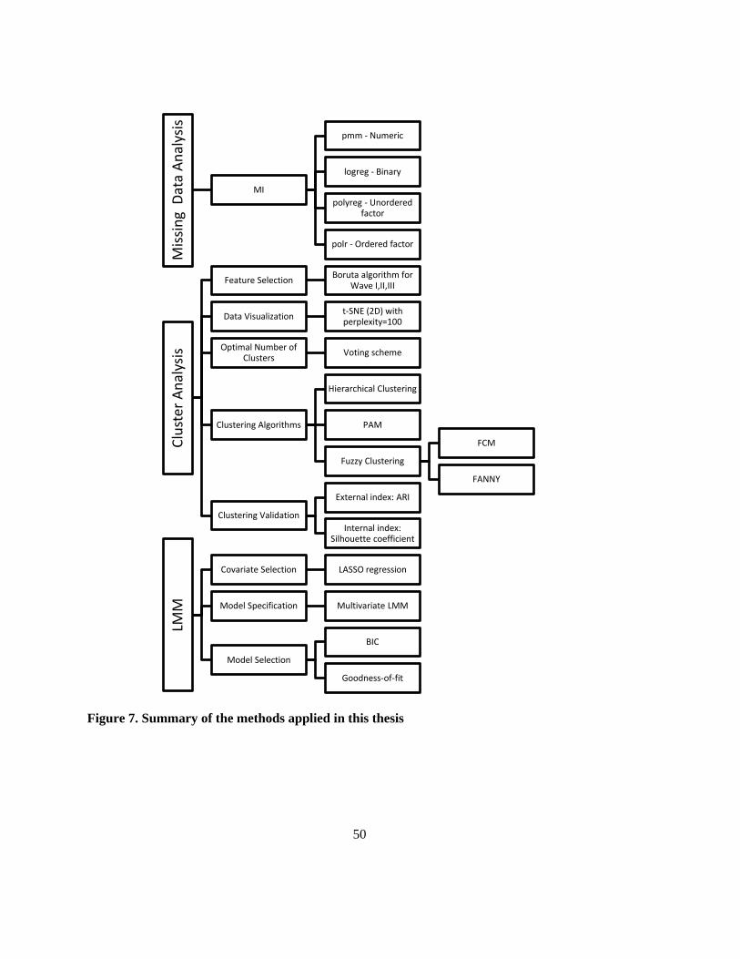
50
Figure 7. Summary of the methods applied in this thesis
Mis
sin
g D
ata
An
alys
isMI
pmm - Numeric
logreg - Binary
polyreg - Unordered factor
polr - Ordered factor
Clu
ster
An
alys
is
Feature SelectionBoruta algorithm for
Wave I,II,III
Data Visualizationt-SNE (2D) with perplexity=100
Optimal Number of Clusters
Voting scheme
Clustering Algorithms
Hierarchical Clustering
PAM
Fuzzy Clustering
FCM
FANNY
Clustering Validation
External index: ARI
Internal index: Silhouette coefficient
LMM
Covariate Selection LASSO regression
Model Specification Multivariate LMM
Model Selection
BIC
Goodness-of-fit

51
Chapter 5
Results
This chapter presents the results of this thesis in the following seven sections. Section 5.1 reports the
results of data preprocessing, followed by descriptive statistics of the linked three waves data
presented in Section 5.2. Sections 5.3 and 5.4 report the clustering and LMM modelling results.
Sections 5.5 through 5.7 present the risk profiles of youth polysubstance use, the patterns of
polysubstance use among Canadian secondary school students, and the dynamic transitions of these
use patterns across time.
5.1 Data Preprocessing
5.1.1 Missing Data Analysis
The overall percentage of missing values for the three waves linked data were 14.5%, 2.3%, and 2.1%
for Wave I, Wave II, and Wave III, respectively. The much higher missingness for Wave I data was
because questions regarding mental health-related (FLOURISH, GAD7, CESD, and DERS) and
online gambling were not asked in the Year 5 survey questionnaire. Aside from these, BMI and
SupportQuitDrugAlcohol variables accounted for 27.1% and 4.2% of total missingness for Wave I.
BMI, CESD, and GAD7 were identified as the top 3 missingness for Wave II and Wave III datasets,
with 22.6%, 11.6%, and 5.8% of total missingness for Wave II, and 18.2%, 10.1%, and 5.4% of total
missingness for Wave III data, respectively.
Fortunately, the missingness of substance use indicators was much less than those of the other
features in all three wave datasets. For example, there were only 237, 122, and 136 missing responses
to the substance use variables at Wave I, Wave II, and Wave III, accounting for 2.5%, 1.3%, and
1.5% of total missingness, respectively. The missing values were omitted during cluster analysis due
to the low missingness of these variables of interest. Since LMMs can facilitate multivariate
responses by treating the missingness as MAR. Thus, missing values for these response variables
were not imputed prior to fitting the LMMs. This approach can maximize the use of linked data with
missing responses at the time occasions of measurement. See Appendix J for a detailed illustration of
the amount of missing data and the missing patterns (i.e., the combinations of missingness across

52
observations) for each wave. The plots of the missing patterns of substance use indicators can be seen
in Appendix J as well.
Figures 8-10 demonstrate the distribution of imputed data for each wave. It is observed that the five
imputed datasets (as represented in red lines) had a reasonably consistent distribution as the original
dataset with no missing values (as described in a blue line) for each feature.
Figure 8. Density plot of imputed data by feature (Wave I, 2016-17)

53
Figure 9. Density plot of imputed data by feature (Wave II, 2017-18)
Figure 10. Density plot of imputed data by feature (Wave III, 2018-19)

54
5.2 Descriptive Statistics
Of the 8824 linked samples collected from the COMPASS study of grades 7 to 10 Canadian
secondary school students at Wave I, 54.6% were females while 45.4% were males, and 74.2% were
white. Grades 9 and 10 students accounted for 50.9% and 34.2% of the total linked sample size,
respectively. 67.5% of the students were from Ontario, and 54.3% live in large urban areas. In terms
of cigarette smoking in the last 30 days, 90% responded as having never smoked, while 6.6%
admitted to smoking occasionally, and 2.8% identified as current smokers. 82% of the students
admitted that they have never used an e-cigarette, while those who acknowledged themselves as
occasional and current users of e-cigarette accounted for 10.1% and 6.5%, respectively. 61.2% of the
students indicated that they never had drunk alcohol in the past year, while those admitted to
occasional use and current alcohol use accounted for 20.4% and 17.2%, respectively. Lastly, 88.7%
of the students said they never used marijuana in the past year, while admittance to occasional use
and current use of marijuana accounted for 5.9% and 4.0%, respectively. These frequencies make
sense compared to surveillance data from representative samples. Thus, we are confident that our
linked samples are similar to the youth population in general. Tables 6-7 demonstrate the
characteristics of this linked sample (N = 8824) and the prevalence of each substance used by type
and by wave, respectively.
Table 6. Characteristics of the linked samples
TOTAL
TOTAL N = 8824 100 (%)
Sex Female 4814 54.6
Male 4010 45.4
Grade 7 691 7.8
8 628 7.1
9 4487 50.9
10 3018 34.2
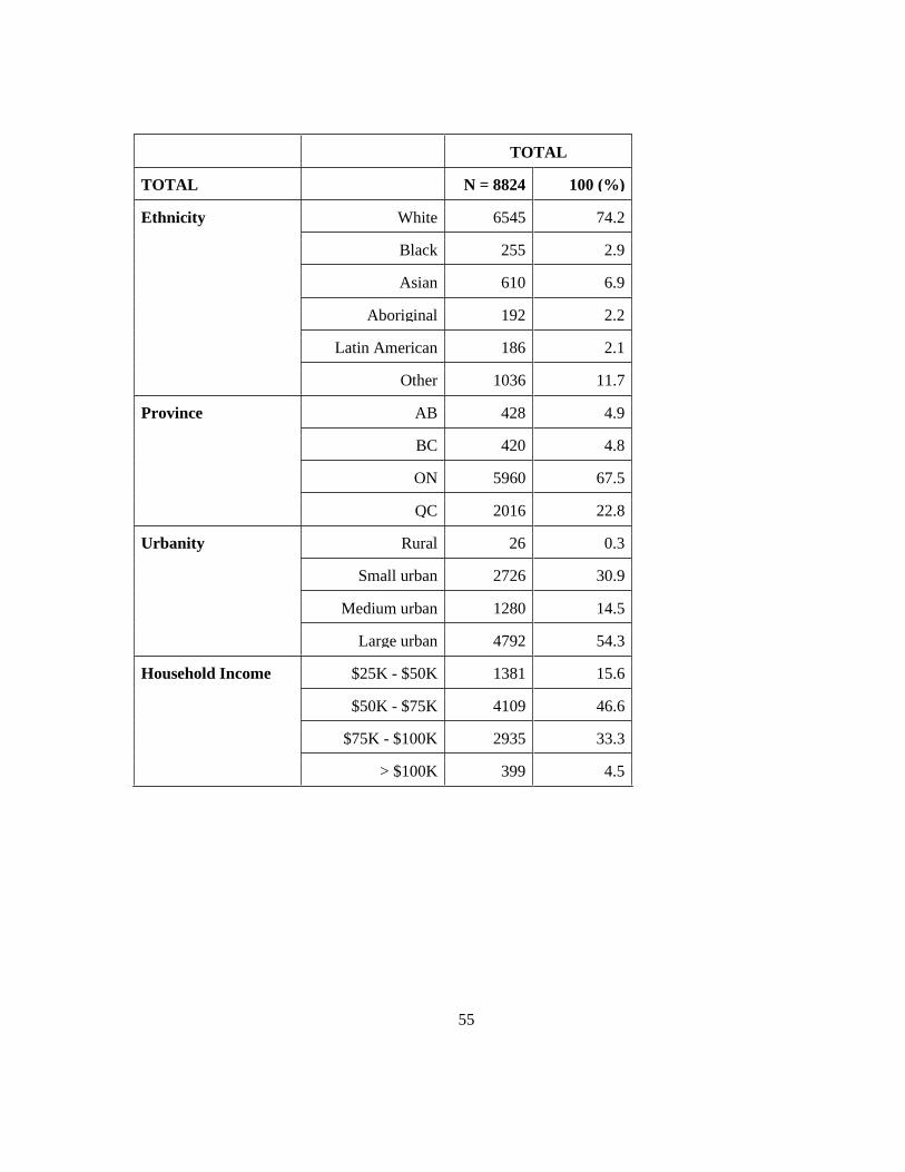
55
TOTAL
TOTAL N = 8824 100 (%)
Ethnicity White 6545 74.2
Black 255 2.9
Asian 610 6.9
Aboriginal 192 2.2
Latin American 186 2.1
Other 1036 11.7
Province AB 428 4.9
BC 420 4.8
ON 5960 67.5
QC 2016 22.8
Urbanity Rural 26 0.3
Small urban 2726 30.9
Medium urban 1280 14.5
Large urban 4792 54.3
Household Income $25K - $50K 1381 15.6
$50K - $75K 4109 46.6
$75K - $100K 2935 33.3
> $100K 399 4.5

56
Table 7. Prevalence of each substance used by type and by wave
Substance Use
Indicator
Label Wave I (2016-17)
Frequency (%)
Wave II (2017-18)
Frequency (%)
Wave III (2018-19)
Frequency (%)
Cigarette Never use 7944 (90.0) 7310 (82.8) 6728 (76.2)
Occasional use 580 (6.6) 974 (11.0) 1437 (16.3)
Current use 250 (2.8) 508 (5.8) 615 (7.0)
Missing 50 (0.6) 32 (0.4) 44 (0.5)
E-Cigarette Never use 7238 (82.0) 5982 (67.8) 4403 (49.9)
Occasional use 889 (10.1) 1195 (13.5) 1525 (17.3)
Current use 577 (6.5) 1589 (18.0) 2834 (32.1)
Missing 120 (1.4) 58 (0.7) 62 (0.7)
Alcohol Never use 5400 (61.2) 3710 (42.0) 2573 (29.2)
Occasional use 1799 (20.4) 2490 (28.2) 2684 (30.4)
Current use 1515 (17.2) 2565 (29.1) 3501 (39.7)
Missing 110 (1.2) 59 (0.7) 66 (0.7)
Marijuana Never use 7831 (88.7) 6784 (76.9) 5569 (63.1)
Occasional use 521 (5.9) 1162 (13.2) 1784 (20.2)
Current use 357 (4.0) 820 (9.3) 1401 (15.9)
Missing 115 (1.3) 58 (0.7) 70 (0.8)
Figures 11-14 are 3D graphs of substance use prevalence by type and wave for cigarettes, e-
cigarette, alcohol, and marijuana use. The overall trend shows that, in general, the prevalence of
“never use” had been decreasing over time, while the prevalence of “occasional use” and “current
use” had been increasing for all substances across the three waves. In particular, as demonstrated in
Figures 12 and 14, respectively, the prevalence of current use for e-cigarette and marijuana
consumption had increased significantly. E-cigarette use increased by 4.94 times from 6.5% in 2016
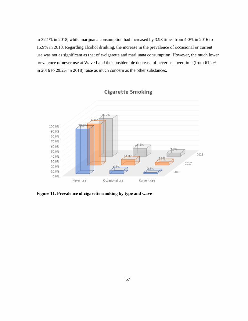
57
to 32.1% in 2018, while marijuana consumption had increased by 3.98 times from 4.0% in 2016 to
15.9% in 2018. Regarding alcohol drinking, the increase in the prevalence of occasional or current
use was not as significant as that of e-cigarette and marijuana consumption. However, the much lower
prevalence of never use at Wave I and the considerable decrease of never use over time (from 61.2%
in 2016 to 29.2% in 2018) raise as much concern as the other substances.
Figure 11. Prevalence of cigarette smoking by type and wave
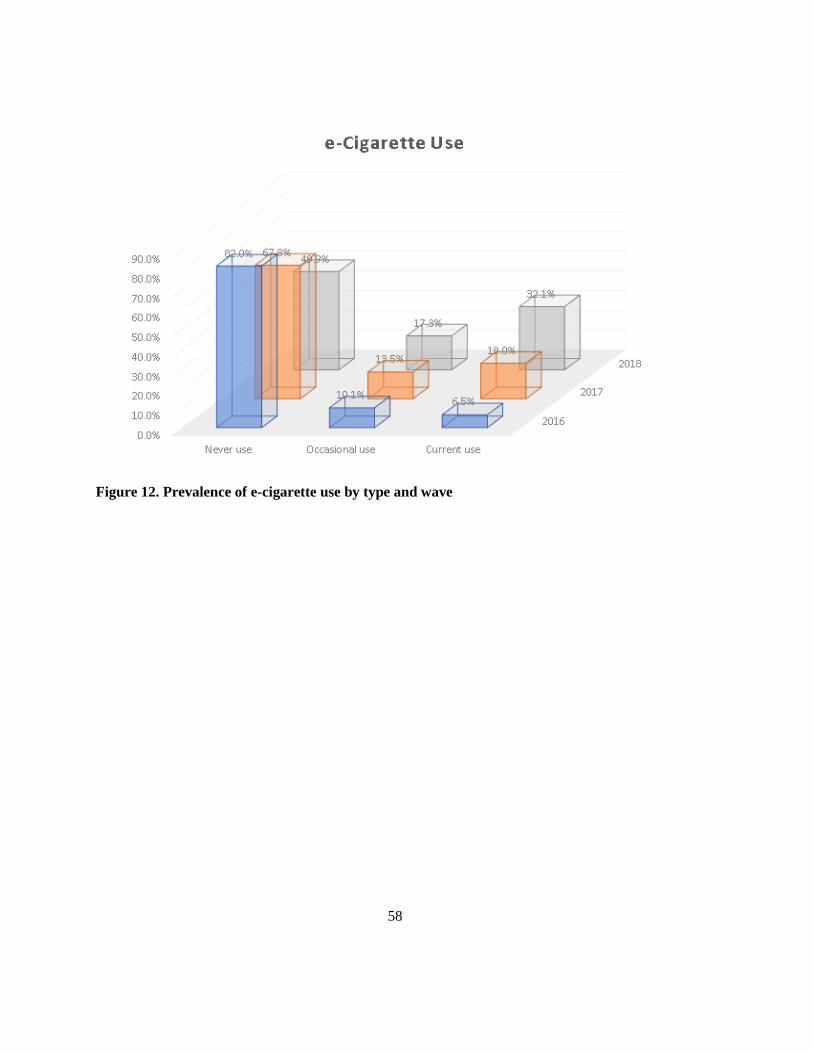
58
Figure 12. Prevalence of e-cigarette use by type and wave
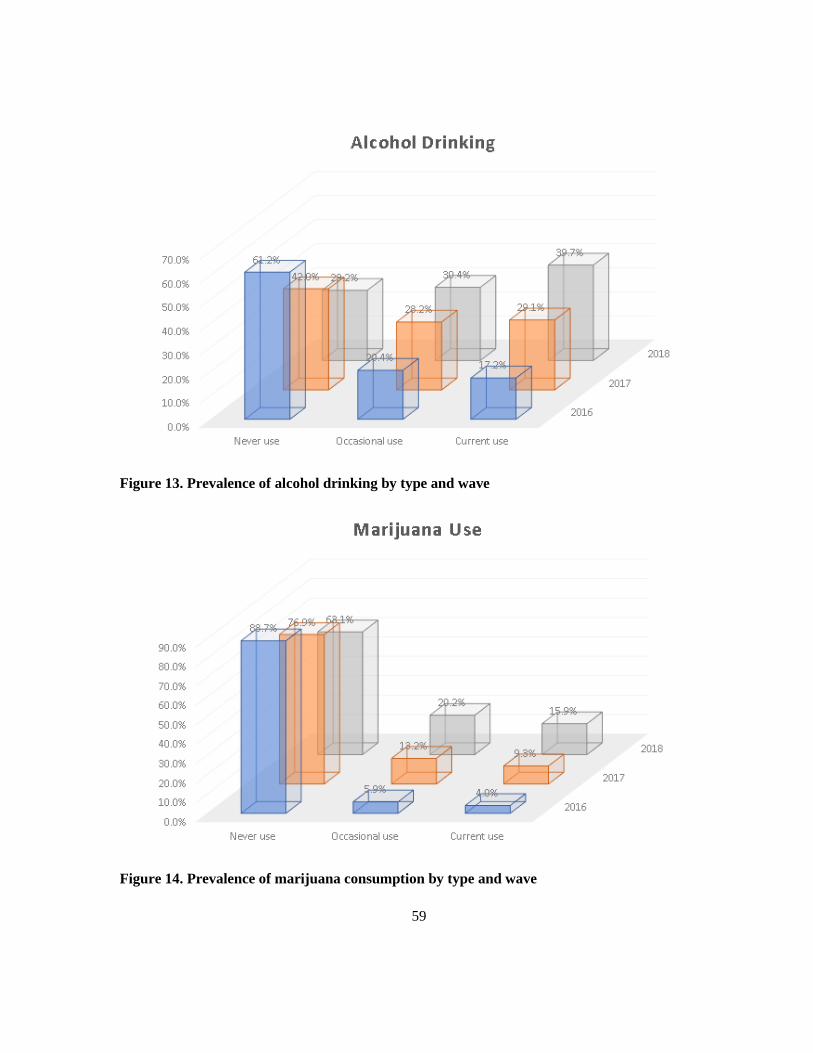
59
Figure 13. Prevalence of alcohol drinking by type and wave
Figure 14. Prevalence of marijuana consumption by type and wave
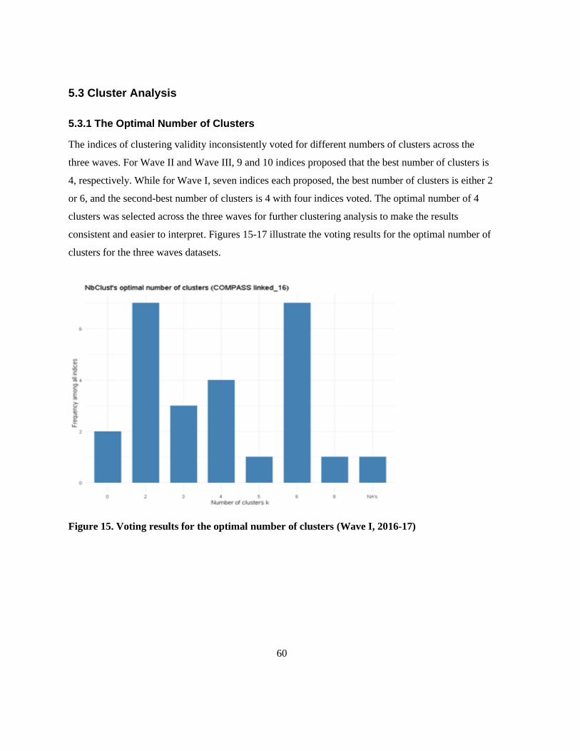
60
5.3 Cluster Analysis
5.3.1 The Optimal Number of Clusters
The indices of clustering validity inconsistently voted for different numbers of clusters across the
three waves. For Wave II and Wave III, 9 and 10 indices proposed that the best number of clusters is
4, respectively. While for Wave I, seven indices each proposed, the best number of clusters is either 2
or 6, and the second-best number of clusters is 4 with four indices voted. The optimal number of 4
clusters was selected across the three waves for further clustering analysis to make the results
consistent and easier to interpret. Figures 15-17 illustrate the voting results for the optimal number of
clusters for the three waves datasets.
Figure 15. Voting results for the optimal number of clusters (Wave I, 2016-17)
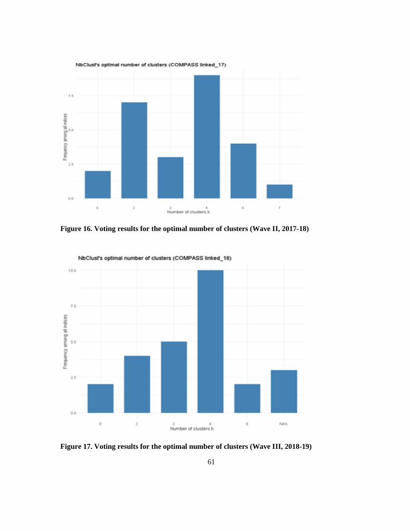
61
Figure 16. Voting results for the optimal number of clusters (Wave II, 2017-18)
Figure 17. Voting results for the optimal number of clusters (Wave III, 2018-19)

62
5.3.2 Clustering Results
5.3.2.1 Fuzzy (FANNY) Clustering
The left panels of Figures 18-20 demonstrate the 2D representation of the student data with coloured
cluster membership based on the fuzzy (FANNY) clustering. The cluster subgroups ranged from 986
to 2799 students at Wave I, 684 to 3082 at Wave II, and 686 to 3385 at Wave III. It is observed that
except for the minority group with the lowest silhouette value, the average silhouette width for all
clusters was positive. The average silhouette widths were 0.52, 0.53, and 0.53 at Wave I, Wave II,
and Wave III, respectively. The silhouette values for each cluster ranged from 0.31 to 0.57 at Wave I,
0.35 to 0.58 at Wave II, and 0.30 to 0.56 at Wave III. Kaufman et al. (2009) proposed that the
silhouette values between 0.71 and 1 indicate a strong structure for that particular cluster (129).
Reasonable and weak structures are shown by the silhouette values between 0.51 and 0.70 and below
0.50, respectively. The two clusters with the second-largest and largest sample size had reasonable
structures, whereas the other two with the smallest and the second smallest sample size had weak
structures at Wave I and II. As for Wave III, three clusters had reasonable structures, and only one
cluster with the smallest sample size had a weak structure. The right panels of Figures 18-20
demonstrate the average silhouette widths for all clusters. These clustering results support the
applicability of phenotyping risk profiles of youth polysubstance use.
Figure 18. Fuzzy (FANNY) Clustering, left-panel: 2D representation; right-panel: silhouette
plot (Wave I, 2016-17)

63
Figure 19. Fuzzy (FANNY) Clustering, left-panel: 2D representation; right-panel: silhouette
plot (Wave II, 2017-18)
Figure 20. Fuzzy (FANNY) Clustering, left-panel: 2D representation; right-panel: silhouette
plot (Wave III, 2018-19)
5.3.2.2 FCM Clustering
The cluster subgroups ranged from 1042 to 3312 students at Wave I, 994 to 3390 at Wave II, and 863
to 3607 at Wave III. Similar to the FANNY algorithm of fuzzy clustering, the average silhouette
widths for all clusters were positive. The average silhouette widths were 0.51 across the three waves.
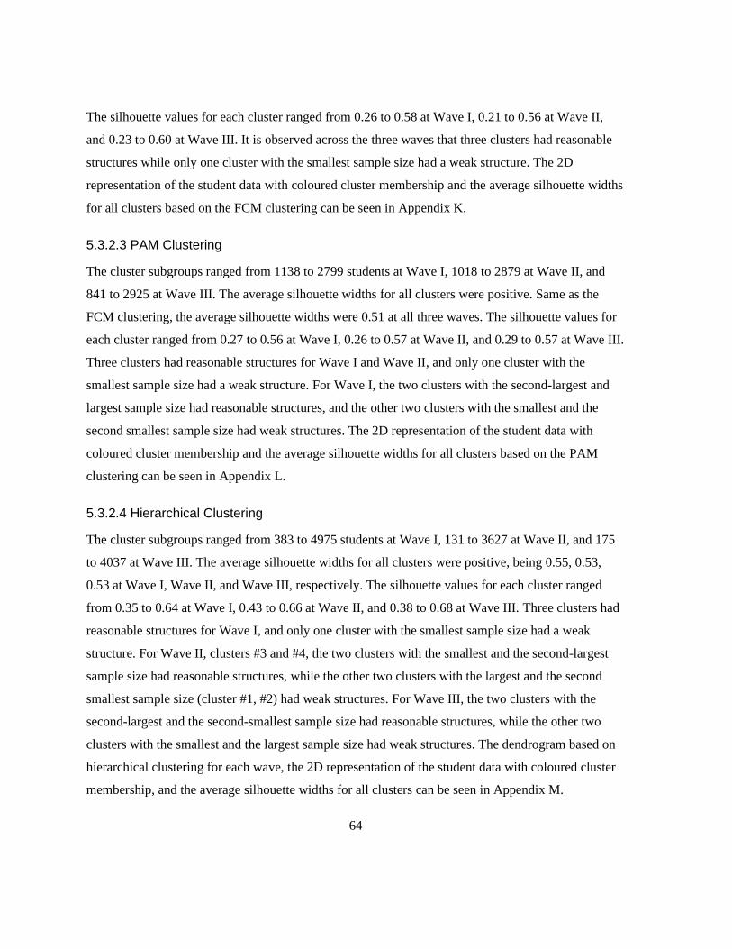
64
The silhouette values for each cluster ranged from 0.26 to 0.58 at Wave I, 0.21 to 0.56 at Wave II,
and 0.23 to 0.60 at Wave III. It is observed across the three waves that three clusters had reasonable
structures while only one cluster with the smallest sample size had a weak structure. The 2D
representation of the student data with coloured cluster membership and the average silhouette widths
for all clusters based on the FCM clustering can be seen in Appendix K.
5.3.2.3 PAM Clustering
The cluster subgroups ranged from 1138 to 2799 students at Wave I, 1018 to 2879 at Wave II, and
841 to 2925 at Wave III. The average silhouette widths for all clusters were positive. Same as the
FCM clustering, the average silhouette widths were 0.51 at all three waves. The silhouette values for
each cluster ranged from 0.27 to 0.56 at Wave I, 0.26 to 0.57 at Wave II, and 0.29 to 0.57 at Wave III.
Three clusters had reasonable structures for Wave I and Wave II, and only one cluster with the
smallest sample size had a weak structure. For Wave I, the two clusters with the second-largest and
largest sample size had reasonable structures, and the other two clusters with the smallest and the
second smallest sample size had weak structures. The 2D representation of the student data with
coloured cluster membership and the average silhouette widths for all clusters based on the PAM
clustering can be seen in Appendix L.
5.3.2.4 Hierarchical Clustering
The cluster subgroups ranged from 383 to 4975 students at Wave I, 131 to 3627 at Wave II, and 175
to 4037 at Wave III. The average silhouette widths for all clusters were positive, being 0.55, 0.53,
0.53 at Wave I, Wave II, and Wave III, respectively. The silhouette values for each cluster ranged
from 0.35 to 0.64 at Wave I, 0.43 to 0.66 at Wave II, and 0.38 to 0.68 at Wave III. Three clusters had
reasonable structures for Wave I, and only one cluster with the smallest sample size had a weak
structure. For Wave II, clusters #3 and #4, the two clusters with the smallest and the second-largest
sample size had reasonable structures, while the other two clusters with the largest and the second
smallest sample size (cluster #1, #2) had weak structures. For Wave III, the two clusters with the
second-largest and the second-smallest sample size had reasonable structures, while the other two
clusters with the smallest and the largest sample size had weak structures. The dendrogram based on
hierarchical clustering for each wave, the 2D representation of the student data with coloured cluster
membership, and the average silhouette widths for all clusters can be seen in Appendix M.
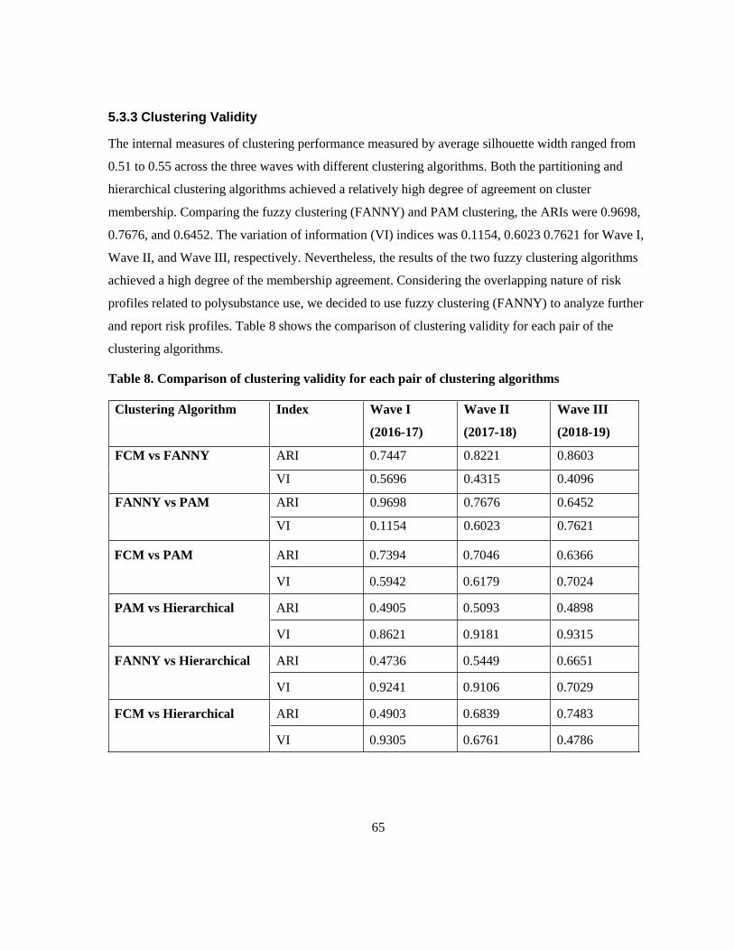
65
5.3.3 Clustering Validity
The internal measures of clustering performance measured by average silhouette width ranged from
0.51 to 0.55 across the three waves with different clustering algorithms. Both the partitioning and
hierarchical clustering algorithms achieved a relatively high degree of agreement on cluster
membership. Comparing the fuzzy clustering (FANNY) and PAM clustering, the ARIs were 0.9698,
0.7676, and 0.6452. The variation of information (VI) indices was 0.1154, 0.6023 0.7621 for Wave I,
Wave II, and Wave III, respectively. Nevertheless, the results of the two fuzzy clustering algorithms
achieved a high degree of the membership agreement. Considering the overlapping nature of risk
profiles related to polysubstance use, we decided to use fuzzy clustering (FANNY) to analyze further
and report risk profiles. Table 8 shows the comparison of clustering validity for each pair of the
clustering algorithms.
Table 8. Comparison of clustering validity for each pair of clustering algorithms
Clustering Algorithm Index Wave I
(2016-17)
Wave II
(2017-18)
Wave III
(2018-19)
FCM vs FANNY ARI 0.7447 0.8221 0.8603
VI 0.5696 0.4315 0.4096
FANNY vs PAM ARI 0.9698 0.7676 0.6452
VI 0.1154 0.6023 0.7621
FCM vs PAM ARI 0.7394 0.7046 0.6366
VI 0.5942 0.6179 0.7024
PAM vs Hierarchical ARI 0.4905 0.5093 0.4898
VI 0.8621 0.9181 0.9315
FANNY vs Hierarchical ARI 0.4736 0.5449 0.6651
VI 0.9241 0.9106 0.7029
FCM vs Hierarchical ARI 0.4903 0.6839 0.7483
VI 0.9305 0.6761 0.4786
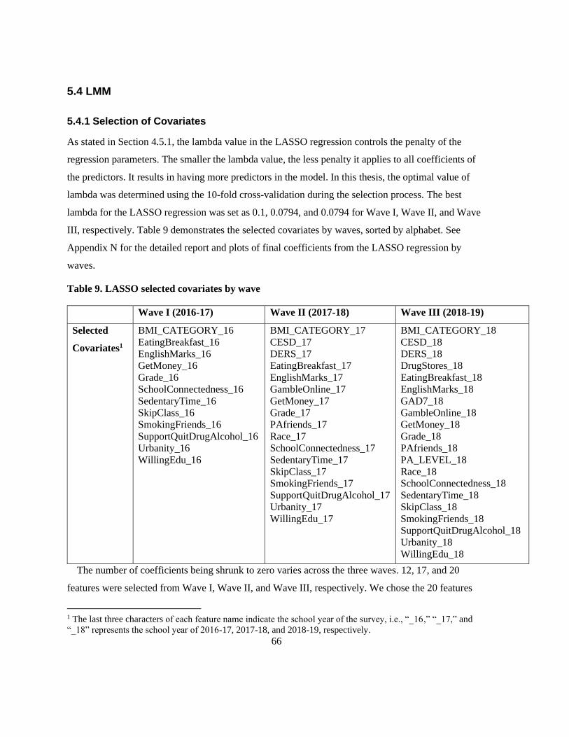
66
5.4 LMM
5.4.1 Selection of Covariates
As stated in Section 4.5.1, the lambda value in the LASSO regression controls the penalty of the
regression parameters. The smaller the lambda value, the less penalty it applies to all coefficients of
the predictors. It results in having more predictors in the model. In this thesis, the optimal value of
lambda was determined using the 10-fold cross-validation during the selection process. The best
lambda for the LASSO regression was set as 0.1, 0.0794, and 0.0794 for Wave I, Wave II, and Wave
III, respectively. Table 9 demonstrates the selected covariates by waves, sorted by alphabet. See
Appendix N for the detailed report and plots of final coefficients from the LASSO regression by
waves.
Table 9. LASSO selected covariates by wave
Wave I (2016-17) Wave II (2017-18) Wave III (2018-19)
Selected
Covariates1
BMI_CATEGORY_16
EatingBreakfast_16
EnglishMarks_16
GetMoney_16
Grade_16
SchoolConnectedness_16
SedentaryTime_16
SkipClass_16
SmokingFriends_16
SupportQuitDrugAlcohol_16
Urbanity_16
WillingEdu_16
BMI_CATEGORY_17
CESD_17
DERS_17
EatingBreakfast_17
EnglishMarks_17
GambleOnline_17
GetMoney_17
Grade_17
PAfriends_17
Race_17
SchoolConnectedness_17
SedentaryTime_17
SkipClass_17
SmokingFriends_17
SupportQuitDrugAlcohol_17
Urbanity_17
WillingEdu_17
BMI_CATEGORY_18
CESD_18
DERS_18
DrugStores_18
EatingBreakfast_18
EnglishMarks_18
GAD7_18
GambleOnline_18
GetMoney_18
Grade_18
PAfriends_18
PA_LEVEL_18
Race_18
SchoolConnectedness_18
SedentaryTime_18
SkipClass_18
SmokingFriends_18
SupportQuitDrugAlcohol_18
Urbanity_18
WillingEdu_18
The number of coefficients being shrunk to zero varies across the three waves. 12, 17, and 20
features were selected from Wave I, Wave II, and Wave III, respectively. We chose the 20 features
1 The last three characters of each feature name indicate the school year of the survey, i.e., “_16,” “_17,” and
“_18” represents the school year of 2016-17, 2017-18, and 2018-19, respectively.

67
from the LASSO regression on Wave III to model the initial probabilities of the latent process. Note
that these 20 features are nested within confirmed features derived from the Boruta algorithm in
clustering analysis. The same 20 covariates and time between occasions (T = 3) were used to model
the transition probabilities, assuming time is heterogeneous, i.e., the dynamics are different across the
three waves. Table 10 summarizes the final selected covariates by level and time-varying status,
sorted by alphabet.
Table 10. Final selected covariates for LMM
Student-Level School-Level
Time-Invariant Race/Ethnicity DrugStores
Urbanity
Time-Varying BMI_CATEGORY
CESD
DERS
EatingBreakfast
EnglishMarks
GAD7
GambleOnline
GetMoney
Grade
PAfriends
PA_LEVEL
SchoolConnectedness
SedentaryTime
SkipClass
SmokingFriends
WillingEdu
SupportQuitDrugAlcohol
A description of the features follows.
BMI_CATEGORY – This is a derived variable representing BMI categories, including 0 = “Not
Stated,” 1 = “Underweight,” 2 = “Healthy Weight,” 3 = “Overweight,” and 4 = “Obese.”
CESD – This is a derived variable, scoring from 0 to 30. In the COMPASS study, depressive
symptoms were assessed using CESD-R-10, the Center for Epidemiologic Studies Depression 10-
Item Scale-Revised. For example, one of the ten scale items was, “On how many of the last 7 days
did you feel the following ways? I was bothered by things that usually don't bother me.” The other
nine items were “I had trouble keeping my mind on what I was doing,” “I felt depressed,” “I felt that
68
everything I did was an effort,” “I felt hopeful about the future,” “I felt fearful,” “My sleep was
restless.” “I was happy,” “I felt lonely,” and “I could not get “going.” The response options were
“None or less than 1 day,” “1-2 days,” “3-4 days,” and “5-7 days.” The response to each of the 10-
items was reverse-scored from 0 to 3 and then summed. The higher the score is, the more significant
depressive symptoms are.
DERS – This is a derived variable, scoring from 6 to 30. In the COMPASS study, difficulties in
regulating emotion were assessed using the Difficulties in Emotion Regulation Scale (DERS). For
example, one of the ten scale items was, “Please indicate how often the following statements apply to
you: I have difficulty making sense out of my feelings.” The response options were “Almost never,”
“Sometimes,” “About half the time,” “Most of the time,” and “Almost always.” The other five items
were “I pay attention to how I feel,” “When I'm upset, I have difficulty concentrating,” “When I'm
upset, I believe there is nothing I can do to make myself feel better,” “When I'm upset, I lose control
over my behaviour,” “When I'm upset, I feel ashamed for feeling that way,” and “Feeling afraid as if
something awful might happen.” The response to each of the 6- items was reverse-scored from 1 to 5
and then summed. The higher the score is, the more complicated an individual is in regulating
emotion.
DrugStores – BE data, the number of drug stores & proprietary stores within 1000 meters of
schools.
EatingBreakfast – Binary indicator variable, 0 = “No” and 1 = “Yes.”
EnglishMarks – Students were asked, “In your current or most recent French/English course, what
is your approximate overall mark? (Think about last year if you have not taken English this year).”
The response options were 1 = “90% - 100%,” 2 = “80% - 89%,” 3 = “70% - 79%,” 4 = “60% -
69%,” 5 = “55% - 59%,” 6 = “50% - 54%,” and 7 = “Less than 50%.”
GAD7 – This is a derived variable, scoring from 0 to 21. In the COMPASS study, generalized
anxiety symptoms were assessed using GAD7, the Generalized Anxiety Disorder 7-item Scale. For
example, one of the seven scale items was, “Over the last 2 weeks, how often have you been bothered
by the following problems? Feeling nervous, anxious, or on edge.” The response options were “Not at
all,” “Several days,” “Over half the days,” and “Nearly every day.” The other six items were “Not
being able to stop or control worrying,” “Worrying too much about different things,” “Trouble

69
relaxing,” “Being so restless that it's hard to sit still,” “Becoming easily annoyed or irritable,” and
“Feeling afraid as if something awful might happen.” The response to each of the 7- items was scored
from 0 to 3 and then summed. The higher the score is, the more severe level of anxiety is per the
GAD-7 scaling.
GambleOnline – Students were asked, “In the last 30 gays, did you gamble online for money?”
The response options are 1 = “Yes” and 2 = “No.”
GetMoney – Students were asked, “About how much money do you usually get each week to
spend on yourself or to save? (Remember to include all money from allowances and jobs like
babysitting, delivering papers, etc.).” The initial responses were categorized into 0 = “I do not know
how much money I get each week,” 1 = “Zero,” 2 = “$1-$20,” 3 = “$21-$100,” and 4 = “$100+.”
Grade – Students were asked, “What grade are you in?” The responses include grades 9-12 and
students in Quebec in secondary 1 and 2 (equivalent to Ontario grades 7 and 8). This variable is a
proxy of students’ age.
PAfriends – Students were asked, “Your closest friends are the friends you like to spend the most
time with. How many of your closest friends are physically active?” The response options are 0 =
“None,” 1 = “1 friend,” 2 = “2 friends,” 3 = “3 friends,” 4 = “4 friends,” and 5 = “5 friends or more.”
PA_LEVEL – This is a derived variable, indicating whether respondents meet the guidelines for at
least 60 minutes of PA per day. Binary variable, 0 = “No” and 1 = “Yes.”
Race/Ethnicity – Students were asked, “How would you describe yourself?” The response options
are 1 = “White,” 2 = “Black,” 3 = “Asian,” 4 = “Aboriginal (First Nations, Métis, Inuit),” 5 = “Latin
American/Hispanic,” and 6 = “Other.”
SchoolConnectedness – This is a derived variable, scoring from 6 to 24. Higher scores indicate
higher connectedness.
SedentaryTime - This is a derived variable representing “Total daily sedentary activity, with
homework excluded,” ranging from 0 to 2925 in minutes.
SkipClass – Students were asked, “In the last 4 weeks, how many classes did you skip when you
were not supposed to?” The response options are 1 = “0 classes,” 2 = “1 or 2 classes,” 3 = “3 to 5
classes,” 4 = “6 to 10 classes,” 5 = “11 to 20 classes,” and 6 = “More than 20 classes.”

70
SmokingFriends – Students were asked, “Your closest friends are the friends you like to spend the
most time with. How many of your closest friends smoke cigarettes?” The response options are 0 =
“None,” 1 = “1 friend,” 2 = “2 friends,” 3 = “3 friends,” 4 = “4 friends,” and 5 = “5 or more friends.”
SupportQuitDrugAlcohol – Students were asked, “How supportive is your school of the
following? Giving students the support they need to resist or quit tobacco.” The response options are
1 = “Very supportive,” 2 = “Supportive,” 3 = “Unsupportive,” and 4 = “Very unsupportive.”
Urbanity – In which the school resides, including “rural,” “small urban,” “medium urban,” and
“large urban.” The urban/rural classification is defined according to the number of populations and
population density per square kilometre (126). The detailed definition of the four categories used in
the COMPASS study is listed in Appendix O.
WillingEdu – Students were asked, “What is the highest level of education you think you will
get?” The response options are 0 = “I don’t know,” 1 = “Some high school or less,” 2 = “High school
diploma or graduation equivalency,” 3 = “College/trade/vocational certificate,” 4 = “University
Bachelor's degree,” and 5 = “University Master’s/PhD/law school/medical school/teachers’ college
degree.”
5.4.2 Selection of the Number of Latent States
Determining the number of latent states was an essential step of the analysis. An increasing number of
latent statuses between 1 and 6 was fitted to a multivariate LMM, assuming that: i) the conditional
response probabilities are time homogenous and are independent of the included covariates, ii) the
probability of using a substance is constrained to 0 for the first latent state; iii) the initial probabilities
are distinct for any categories of the included covariates, and iv) the transition probabilities are time
heterogeneous and distinct for any categories of the included covariates.
The information criteria provided slightly different results of which model best balances model fit
and parsimony. The BIC value indicated that the model with four latent statuses is preferred, whereas
the AIC value pointed to a preferable six latent states. Since BIC is a more reliable criterion (27) and
considers parsimony, conceptual appeal, and more straightforward interpretation, the 4-latent-status
model was selected for further analysis. Figure 21 shows the BIC and AIC criteria for the multivariate
LMM.
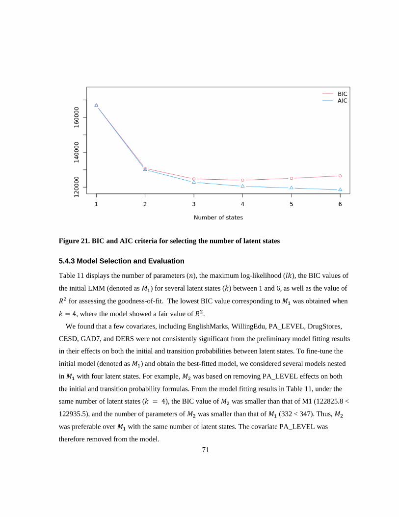
71
Figure 21. BIC and AIC criteria for selecting the number of latent states
5.4.3 Model Selection and Evaluation
Table 11 displays the number of parameters (𝑛), the maximum log-likelihood (𝑙𝑘), the BIC values of
the initial LMM (denoted as 𝑀1) for several latent states (𝑘) between 1 and 6, as well as the value of
𝑅2 for assessing the goodness-of-fit. The lowest BIC value corresponding to 𝑀1 was obtained when
𝑘 = 4, where the model showed a fair value of 𝑅2.
We found that a few covariates, including EnglishMarks, WillingEdu, PA_LEVEL, DrugStores,
CESD, GAD7, and DERS were not consistently significant from the preliminary model fitting results
in their effects on both the initial and transition probabilities between latent states. To fine-tune the
initial model (denoted as 𝑀1) and obtain the best-fitted model, we considered several models nested
in 𝑀1 with four latent states. For example, 𝑀2 was based on removing PA_LEVEL effects on both
the initial and transition probability formulas. From the model fitting results in Table 11, under the
same number of latent states (𝑘 = 4), the BIC value of 𝑀2 was smaller than that of M1 (122825.8 <
122935.5), and the number of parameters of 𝑀2 was smaller than that of 𝑀1 (332 < 347). Thus, 𝑀2
was preferable over 𝑀1 with the same number of latent states. The covariate PA_LEVEL was
therefore removed from the model.

72
Similarly, the other covariates EnglishMarks, WillingEdu, and SedentaryTime, were removed from
model fitting one by one and by pairs. That is how the models 𝑀2 ~ 𝑀18 were fitted, assuming that
certain covariate(s) do not affect the initial and the transition probabilities of the latent process.
Comparing these models with 𝑀1, it is concluded that EnglishMarks, WillingEdu, PA_ LEVEL,
DrugStores, CESD, GAD7, and DERS did not significantly affect these probabilities. The model was
formulated by removing these covariates, denoted by 𝑀16.
Although sex was not identified as an important predictor by the LASSO regression, the literature
review on the risk factors of youth polysubstance use indicates its inconsistent effects from various
studies; it was determined as a factor worth investigating as a predictor. Therefore, we decided to
include the covariate sex into LMMs as one of the time-invariant covariates (𝑀17 and 𝑀18). In the
COMPASS dataset, sex was dummy coded as 1 = “Female” and 2 = “Male” across all waves. Since
further simplification significantly increased the BIC value, 𝑀18 was selected as the final model.
Among all the fitted models, 𝑀18 had the lowest BIC, which equals 122349.6. Under this model, the
maximum log-likelihood equals -60007.4 with 257 parameters, and a fair value of the index 𝑅2 was
obtained. Table 11 summarizes the preliminary fitting of the LMMs with different values of 𝑘 and
various constraints discussed in this section.
Table 11. Preliminary fitting of various LMMs
Model k n lk BIC R2
𝑀1 1 8 -83391.2 166855.1
2 79 -64967.2 130652 0.4067
3 192 -61218.2 124180.8 0.4664
4 347 -59891.5 122935.5 0.4861
5 544 -59168.5 123279.3 0.4966
6 783 -58391.4 123896.5 0.5075
𝑀2: 𝑀1 – PA_LEVEL 4 332 -59904.8 122825.8 0.4859
𝑀3: 𝑀1 – GAD7 4 332 -59908 122832.4 0.4859
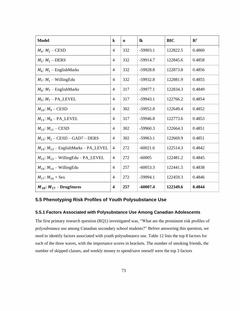
73
Model k n lk BIC R2
𝑀4: 𝑀1 – CESD 4 332 -59903.1 122822.5 0.4860
𝑀5: 𝑀1 – DERS 4 332 -59914.7 122845.6 0.4858
𝑀6: 𝑀1 – EnglishMarks 4 332 -59928.8 122873.8 0.4856
𝑀7: 𝑀1 – WillingEdu 4 332 -59932.8 122881.9 0.4855
𝑀8: 𝑀7 – EnglishMarks 4 317 -59977.1 122834.3 0.4849
𝑀9: 𝑀7 – PA_LEVEL 4 317 -59943.1 122766.2 0.4854
𝑀10: 𝑀9 – CESD 4 302 -59952.8 122649.4 0.4852
𝑀11: 𝑀8 – PA_LEVEL 4 317 -59946.8 122773.6 0.4853
𝑀12: 𝑀11 – CESD 4 302 -59960.3 122664.3 0.4851
𝑀13: 𝑀1 – CESD – GAD7 – DERS 4 302 -59963.1 122669.9 0.4851
𝑀14: 𝑀13 – EnglishMarks – PA_LEVEL 4 272 -60021.6 122514.3 0.4842
𝑀15: 𝑀13 – WillingEdu – PA_LEVEL 4 272 -60005 122481.2 0.4845
𝑀16: 𝑀14 – WillingEdu 4 257 -60053.3 122441.5 0.4838
𝑀17: 𝑀16 + Sex 4 272 -59994.1 122459.3 0.4846
𝑴𝟏𝟖: 𝑴𝟏𝟕 – DrugStores 4 257 -60007.4 122349.6 0.4844
5.5 Phenotyping Risk Profiles of Youth Polysubstance Use
5.5.1 Factors Associated with Polysubstance Use Among Canadian Adolescents
The first primary research question (RQ1) investigated was, “What are the prominent risk profiles of
polysubstance use among Canadian secondary school students?” Before answering this question, we
need to identify factors associated with youth polysubstance use. Table 12 lists the top 8 factors for
each of the three waves, with the importance scores in brackets. The number of smoking friends, the
number of skipped classes, and weekly money to spend/save oneself were the top 3 factors

74
consistently appearing across the three waves. Other correlates ranked differently by waves. The total
importance scores for each factor can be seen in the last column of Table 12.
Table 12. Top 8 factors associated with polysubstance use by wave
Ranki
ng
Wave I
(2016-17)
Wave II
(2017-18)
Wave III
(2018-19)
Voting
(Total Score)
1 SmokingFriends_16
(47.92)
SmokingFriends_17
(60.05)
SmokingFriends
_18 (56.90)
SmokingFriends
(164.87)
2 SkipClass_16 (38.01) SkipClass_17 (43.76) SkipClass_18
(54.12)
SkipClass
(135.89)
3 GetMoney_16 (17.48) GetMoney_17
(31.07)
GetMoney_18
(37.66)
GetMoney (86.21)
4 SchoolConnectedness_1
6 (16.65)
SedentaryTime_17
(20.12)
SedentaryTime_
18 (20.26)
SedentaryTime
(53.14)
5 Grade_16 (15.58) CESD_17 (15.87) EatingBreakfast
_18 (19.03)
CESD (42.74)
6 CESD_16 (14.19) SchoolConnectednes
s_17 (14.29)
PAfriends_18
(17.41)
SchoolConnected
ness (42.51)
7 Province_16 (13.38) Urbanity_17 (13.95) EnglishMarks_1
8 (15.16)
EatingBreakfast
(38.29)
8 SedentaryTime_16
(12.76)
EatingBreakfast_17
(13.32)
Urbanity_18
(14.95)
Grade/Age
(38.05)
Figures 22-24 illustrate variable importance by waves. X-axis and Y-axis represent variables and
importance, respectively. The higher value of Y, the more important the corresponding variable was.
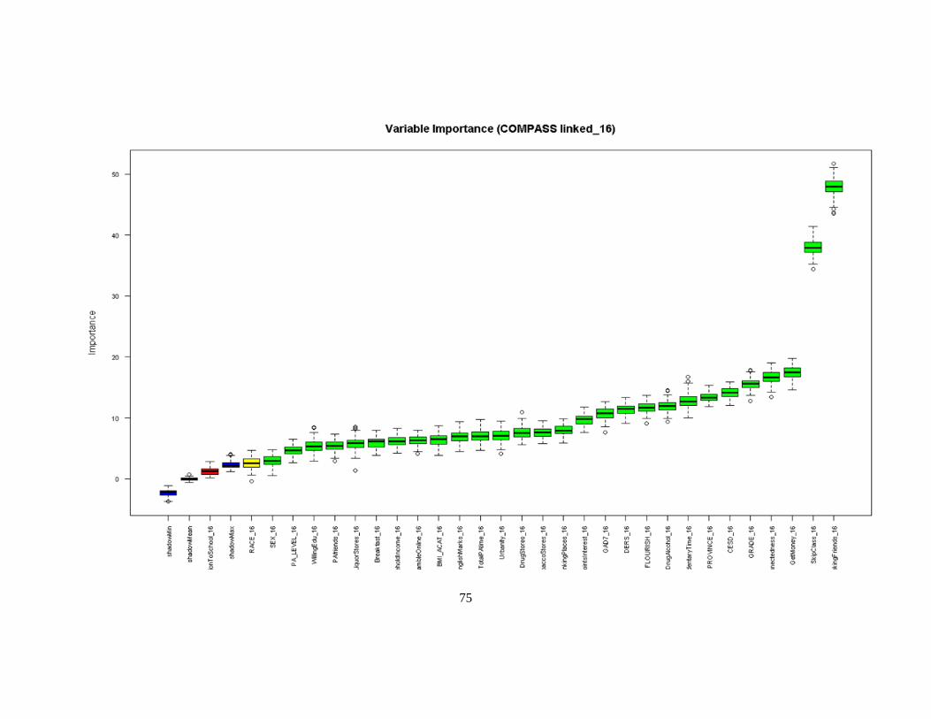
75
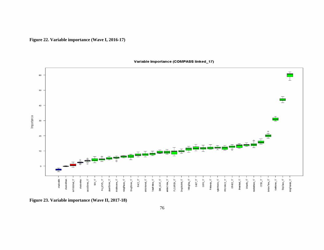
76
Figure 22. Variable importance (Wave I, 2016-17)
Figure 23. Variable importance (Wave II, 2017-18)
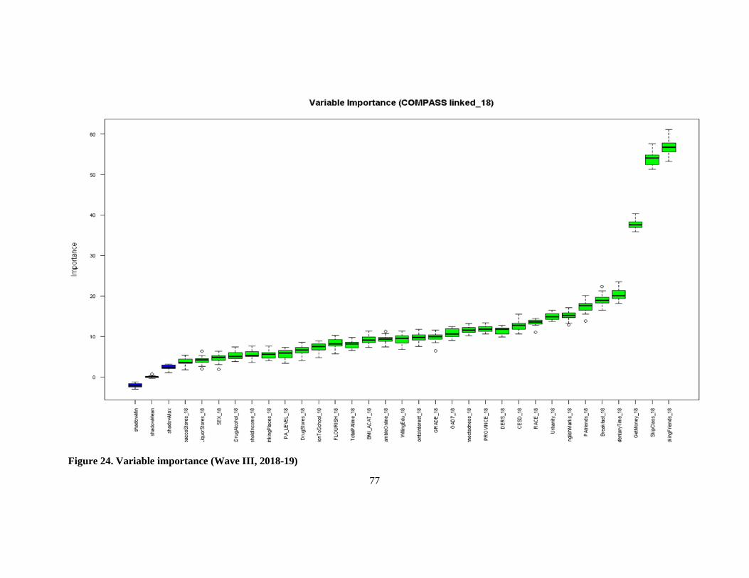
77
Figure 24. Variable importance (Wave III, 2018-19)

78
5.5.2 Risk Profiles of Polysubstance Use Among Canadian Secondary School
Students
Four risk profiles of polysubstance use were identified across the three waves, i.e., low risk (L1),
medium-low risk (L2), medium-high risk (L3), and high risk (L4). This was determined by the
average group score of substance use indicators and the included risk factors. In general, students
with the lowest mean values (scores) of each substance use, CESD and sedentary time, fewest
smoking friends, fewest skipped classes, highest mean scores of school connectedness, and the
majority eating breakfast were in the low-risk group. On the contrary, those majority who reported
not eating breakfast, with the lowest mean scores of school connectedness, highest mean values
(scores) of each substance use, CESD and sedentary time, a larger number of smoking friends, and a
higher number of skipped classes were in the high-risk group. Two intermediate risk profiles were
identified in-between, i.e., medium-low risk and medium-high risk groups. The average group scores
of substance use indicators and risk factors ranged between L1 and L4. Tables 13-15 list the group
mean scores with standard deviation (SD in bracket) of substance use indicators and all risk factors of
these four risk profiles by waves based on fuzzy (FANNY) clustering.
Each of the four substance use indicators was categorized as 0 = “never use,” 1 = “occasional use,”
and 2 = “current use.” These values were treated as continuous scores to fit the Euclidean distance
calculation. That is, the higher scores are indicative of more frequent use of the corresponding
substance. In general, the lower the risk profile, the lower the score of the substance use indicator that
the risk group had. At Wave I, on average, the low-risk (L1) group had the lowest score of indicators
0.06 ± 0.29 (mean ± SD, cigarette smoking), 0.14 ± 0.44 (e-cigarette use), 0.39 ± 0.68 (alcohol
drinking), and 0.06 ± 0.30 (marijuana consumption). Whereas the high-risk (L4) group had the
highest scores of 0.25 ± 0.56 (cigarette smoking), 0.35 ± 0.65 (e-cigarette use), 0.71 ± 0.82 (alcohol
drinking), and 0.29 ± 0.63 (marijuana consumption). The magnitudes comparing L4 vs. L1 are 4.17
(cigarette smoking), 2.5 (e-cigarette use), 1.82 (alcohol drinking), and 4.83 (marijuana consumption)
times at Wave I.
By observing the top risk factor, “the number of smoking friends,” students in the high-risk group
(L4) had the highest score being 0.64 ± 1.21 at Wave I. In contrast, students in the low-risk group
(L1) had the lowest score of 0.19 ± 0.65, significantly differentiating between risk groups. Students at
medium-high (L3) and medium-low (L2) risk groups scored between 0.46 ± 1.03 and 0.31 ± 0.81.

79
The initial values of this variable are categorical, coded as 0 = “None”, 1 = “1 friend”, 2 = “2
friends”, 3 = “3 friends”, 4 = “4 friends”, and 5 = “5 or more friends”. These values were treated as
continuous scores; the higher the score is, the more smoking friends it represents. The magnitudes of
these scores across the four risk groups (Wave III vs. Wave I) are close to each other, ranging from
1.41 times (L3) to 1.68 times (L1) over time.
The difference between students who were at low risk (L1) having, on average, the smallest
sedentary time (170 ± 61.3 minutes) compared to their peers at high risk (L4, 1021 ± 269 minutes)
was by a magnitude of 6.01 times. The sedentary time significantly increased with the increasing risk
profiles, 345 ± 50.7 and 563 ± 83.3 minutes for L2 and L3, respectively. In Wave I data, students in
the L4 group have a CESD score of 10.8 ± 6.70, whereas those in the low-risk group (L1) have the
smallest CESD score of 7.08 ± 5.39, with significant differences between risk groups. The medium-
low (L2) and medium-high (L3) risk groups have moderate CESD scores of 8.34 ± 5.89 and 9.30 ±
6.04, respectively. The same trend is observed in Wave II and III datasets.
The risk profiling reveals that students in the high-risk group (L4) of polysubstance use have the
lowest school connectedness score, 18.0 ± 3.35 at Wave I. In contrast, students in the low-risk group
(L1) have the highest score of 19.8 ± 2.78, significantly different between risk groups. In between,
students in the medium-low (L2) and medium-high risk group (L3) have the scores of school
connectedness being 19.1 ± 2.66 and 18.6 ± 2.81, respectively.
At Wave I, the majority (65.4%) of the participants who ate breakfast were in the low-risk group
(L1), while the majority (68.1%) of the participants in the high-risk group (L4) did not eat breakfast.
The prevalence of eating breakfast decreases while the risk level rises from low-risk (65.4%),
medium-low (51.6%), medium-high (42.4%), to high-risk (31.9%). A similar pattern can be seen
throughout the three waves. The longitudinal evidence suggests that the prevalence of the students
eating breakfast decreased across the three waves in the low-risk group, being 61.7% and 55.5% at
Wave II and Wave III. In this cohort, the percentage of students eating breakfast at Wave III (55.5%)
was 0.85 times less than that of Wave I (65.4%), indicating a decrease over time. The same trend was
observed among the other three risk profile groups (L2 to L4). Comparing the other three risk profiles
(Wave III vs. Wave I), the differences were similar to that of L1, being 0.81 times (L2), 0.79 times
(L3), and 0.78 times (L4).
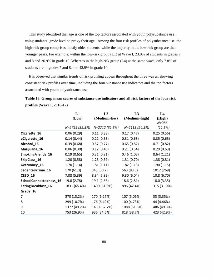
80
This study identified that age is one of the top factors associated with youth polysubstance use,
using students’ grade level to proxy their age. Among the four risk profiles of polysubstance use, the
high-risk group comprises mostly older students, while the majority in the low-risk group are their
younger peers. For example, within the low-risk group (L1) at Wave I, 23.9% of students in grades 7
and 8 and 26.9% in grade 10. Whereas in the high-risk group (L4) at the same wave, only 7.8% of
students are in grades 7 and 8, and 42.9% in grade 10.
It is observed that similar trends of risk profiling appear throughout the three waves, showing
consistent risk profiles over time, including the four substance use indicators and the top factors
associated with youth polysubstance use.
Table 13. Group mean scores of substance use indicators and all risk factors of the four risk
profiles (Wave I, 2016-17)
L1
(Low) L2
(Medium-low) L3
(Medium-high) L4
(High)
N=2799 (32.5%) N=2712 (31.5%) N=2113 (24.5%) N=986 (11.5%)
Cigarette_16 0.06 (0.29) 0.11 (0.38) 0.17 (0.47) 0.25 (0.56)
eCigarette_16 0.14 (0.44) 0.22 (0.55) 0.31 (0.63) 0.35 (0.65)
Alcohol_16 0.39 (0.68) 0.57 (0.77) 0.65 (0.82) 0.71 (0.82)
Marijuana_16 0.06 (0.30) 0.12 (0.40) 0.21 (0.54) 0.29 (0.63)
SmokingFriends_16 0.19 (0.65) 0.31 (0.81) 0.46 (1.03) 0.64 (1.21)
SkipClass_16 1.20 (0.58) 1.23 (0.59) 1.31 (0.70) 1.38 (0.81)
GetMoney_16 1.70 (1.14) 1.81 (1.11) 1.82 (1.13) 1.90 (1.15)
SedentaryTime_16 170 (61.3) 345 (50.7) 563 (83.3) 1012 (269)
CESD_16 7.08 (5.39) 8.34 (5.89) 9.30 (6.04) 10.8 (6.70)
SchoolConnectedness_16 19.8 (2.78) 19.1 (2.66) 18.6 (2.81) 18.0 (3.35)
EatingBreakfast_16 1831 (65.4%) 1400 (51.6%) 896 (42.4%) 315 (31.9%)
Grade_16
7 370 (13.2%) 170 (6.27%) 107 (5.06%) 33 (3.35%)
8 299 (10.7%) 176 (6.49%) 100 (4.73%) 44 (4.46%)
9 1377 (49.2%) 1430 (52.7%) 1088 (51.5%) 486 (49.3%)
10 753 (26.9%) 936 (34.5%) 818 (38.7%) 423 (42.9%)

81
Table 14. Group mean scores of substance use indicators and all risk factors of the four risk
profiles (Wave II, 2017-18)
L1
(Low) L2
(Medium-low) L3
(Medium-high) L4
(High)
N=3022 (34.7%) N=3082 (35.4%) N=1920 (22.0%) N=684 (7.9%)
Cigarette_17 0.14 (0.43) 0.22 (0.52) 0.29 (0.60) 0.45 (0.72)
eCigarette_17 0.35 (0.68) 0.52 (0.80) 0.61 (0.83) 0.67 (0.85)
Alcohol_17 0.73 (0.80) 0.91 (0.84) 0.96 (0.84) 1.05 (0.86)
Marijuana_17 0.17 (0.48) 0.33 (0.64) 0.43 (0.72) 0.57 (0.78)
SmokingFriends_17 0.28 (0.79) 0.44 (1.01) 0.64 (1.21) 0.94 (1.47)
SkipClass_17 1.28 (0.65) 1.37 (0.76) 1.40 (0.75) 1.62 (1.06)
GetMoney_17 2.06 (1.31) 2.17 (1.32) 2.24 (1.28) 2.24 (1.31)
SedentaryTime_17 193 (64.2) 385 (60.0) 647 (101) 1176 (308)
CESD_17 7.31 (5.54) 8.33 (5.80) 9.37 (5.96) 11.5 (7.07)
SchoolConnectedness_17 19.4 (2.97) 18.7 (3.01) 18.0 (3.15) 17.3 (3.54)
EatingBreakfast_17 1865 (61.7%) 1443 (46.8%) 718 (37.4%) 201 (29.4%)
Grade_17
8 336 (11.1%) 231 (7.50%) 93 (4.84%) 25 (3.65%)
9 302 (9.99%) 207 (6.72%) 87 (4.53%) 24 (3.51%)
10 1415 (46.8%) 1578 (51.2%) 1035 (53.9%) 390 (57.0%)
11 969 (32.1%) 1066 (34.6%) 705 (36.7%) 245 (35.8%)
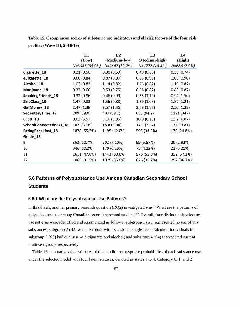
82
Table 15. Group mean scores of substance use indicators and all risk factors of the four risk
profiles (Wave III, 2018-19)
L1
(Low) L2
(Medium-low) L3
(Medium-high) L4
(High)
N=3385 (38.9%) N=2847 (32.7%) N=1776 (20.4%) N=686 (7.9%)
Cigarette_18 0.21 (0.50) 0.30 (0.59) 0.40 (0.66) 0.53 (0.74)
eCigarette_18 0.66 (0.84) 0.87 (0.90) 0.95 (0.91) 1.05 (0.90)
Alcohol_18 1.03 (0.83) 1.14 (0.82) 1.16 (0.82) 1.19 (0.82)
Marijuana_18 0.37 (0.66) 0.53 (0.75) 0.68 (0.82) 0.83 (0.87)
SmokingFriends_18 0.32 (0.86) 0.46 (0.99) 0.65 (1.19) 0.94 (1.50)
SkipClass_18 1.47 (0.83) 1.56 (0.88) 1.69 (1.03) 1.87 (1.21)
GetMoney_18 2.47 (1.38) 2.57 (1.36) 2.58 (1.33) 2.50 (1.32)
SedentaryTime_18 209 (68.0) 403 (58.2) 653 (94.2) 1191 (347)
CESD_18 8.02 (5.57) 9.16 (5.95) 10.0 (6.15) 12.2 (6.87)
SchoolConnectedness_18 18.9 (3.08) 18.4 (3.04) 17.7 (3.32) 17.0 (3.81)
EatingBreakfast_18 1878 (55.5%) 1195 (42.0%) 593 (33.4%) 170 (24.8%)
Grade_18
9 363 (10.7%) 202 (7.10%) 99 (5.57%) 20 (2.92%)
10 346 (10.2%) 179 (6.29%) 75 (4.22%) 22 (3.21%)
11 1611 (47.6%) 1441 (50.6%) 976 (55.0%) 392 (57.1%)
12 1065 (31.5%) 1025 (36.0%) 626 (35.2%) 252 (36.7%)
5.6 Patterns of Polysubstance Use Among Canadian Secondary School
Students
5.6.1 What are the Polysubstance Use Patterns?
In this thesis, another primary research question (RQ2) investigated was, “What are the patterns of
polysubstance use among Canadian secondary school students?” Overall, four distinct polysubstance
use patterns were identified and summarized as follows: subgroup 1 (S1) represented no use of any
substances; subgroup 2 (S2) was the cohort with occasional single-use of alcohol; individuals in
subgroup 3 (S3) had dual-use of e-cigarette and alcohol; and subgroup 4 (S4) represented current
multi-use group, respectively.
Table 16 summarizes the estimates of the conditional response probabilities of each substance use
under the selected model with four latent statuses, denoted as states 1 to 4. Category 0, 1, and 2

83
correspond to the “never use,” “occasional use,” and “current use,” respectively. Predominant
conditional response probabilities with larger values are highlighted in bold font to help with
interpretation. Overall, the conditional response probabilities were well separated, demonstrating
good heterogeneity between subgroups.
Table 16. Conditional response probabilities
Cigarette
Subgroup
Category S1 S2 S3 S4
0 (Never) 0.9910 0.9976 0.7653 0.1494
1 (Occasional) 0.0087 0.0024 0.2114 0.4736
2 (Current) 0.0002 0.0000 0.0232 0.3770
E-Cigarette
Subgroup
Category S1 S2 S3 S4
0 (Never) 0.9637 0.8545 0.2946 0.1115
1 (Occasional) 0.0327 0.1218 0.3249 0.1438
2 (Current) 0.0036 0.0237 0.3805 0.7448
Alcohol
Subgroup
Category S1 S2 S3 S4
0 (Never) 0.9472 0.1048 0.1412 0.0296
1 (Occasional) 0.0528 0.6066 0.3441 0.1755
2 (Current) 0.0000 0.2887 0.5147 0.7949
Marijuana
Subgroup
Category S1 S2 S3 S4
0 (Never) 0.9979 0.9803 0.5453 0.0653
1 (Occasional) 0.0016 0.0196 0.3553 0.3337
2 (Current) 0.0005 0.0001 0.0994 0.6010

84
Figure 25 illustrates conditional response probabilities involving multivariate response categories.
Each subgroup was determined by the predominant conditional response probabilities of the
substance use(s). The latent status can be explained based on the corresponding distribution of the
response variables in the parameter estimation.
Figure 25. Conditional response probabilities
It is observed that Class 1 (S1) corresponds to students with no use of any substances, where the
probability of the first category (never use) was greater than 94.7% for any substance. Class 2 (S2)
was composed of individuals who typically used alcohol on an occasional basis. This is due to a more
significant probability of occasional alcohol drinking (60.7%), whereas over 85.5% of probabilities
never used the other three substances in this subgroup. Individuals in Class 3 (S3) had larger
probabilities of occasional and current use of e-cigarette and alcohol, being 70.5% and 85.9%,
respectively. The probabilities of using other substances in this subgroup were not prominent,
although there were 21.1% and 35.5% of probabilities of smoking cigarettes and consuming
marijuana, respectively. Individuals in Class 4 (S4) differed from those in S3 by having a greater
probability of using multiple substances concurrently. For instance, the conditional response

85
probabilities of current e-cigarette use, alcohol drinking, and marijuana consumption were 74.5%,
79.5%, and 60.1%, respectively. Thus, S4 corresponds to the heavy multi-user group.
At the beginning of the observation period, the initial probabilities of each use pattern were 0.5887,
0.2156, 0.1487, and 0.0470, representing the chance of being in the no-use (S1), occasional single-use
of alcohol (S2), dual-use of e-cigarette and alcohol (S3), and multi-use (S4) subgroup, respectively.
The sizes of each use pattern are summarized in Table 17. In particular, S1 was the largest subgroup,
containing 5320 students, accounting for 60.3% of the total sample size (N = 8824) at Wave I,
followed by S2 (21.1%) and S3 (14.1%). Lastly, S4, the highest risk group, comprising current multi-
use of substance users, consisted of 399 students, accounting for 4.5% of the total sample size at
Wave I.
Table 17. Size of each pattern at Wave I (2016-17)
Count %
Wave I (2016-17)
S1: No-use 5320 60.3
S2: Occasional single-use (A) 1859 21.1
S3: Dual-use (E+A) 1246 14.1
S4: Multi-use 399 4.5
Grand Total 8824 100.0
5.6.2 What Factors are Associated with Patterns of Polysubstance Use?
Associated with the primary research question RQ2, a secondary research question (RQ4) examined
was, “What factors are associated with patterns of polysubstance use among Canadian adolescents?”
We estimated the covariates' effects on their initial probabilities to investigate the factors associated
with the diverse use patterns of substances among youth. Table 18 lists the coefficients of all
predictors with corresponding odds ratios (OR) affecting the initial probabilities for each use pattern
membership under the selected model. To evaluate the significance of predictors on the effect of
subgroup membership for the initial probabilities, Wald test statistics (t-test) was performed based on

86
the parameter estimates and standard errors. Corresponding p-values were obtained, as shown in
Table 18 below.
Table 18. Predictors of subgroup membership for the initial probabilities at Wave I (Ref: S1)
Subgroup
S2 S3 S4
intercept
β (beta coefficient) -0.84 -0.54 -0.44
Odds Ratios 0.43*** 0.58*** 0.65***
Urbanity
β (beta coefficient) -0.20 -0.27 -0.42
Odds Ratios 0.82*** 0.77*** 0.66***
Grade/Age
β (beta coefficient) 0.28 0.23 0.41
Odds Ratios 1.32*** 1.26*** 1.51***
Race/Ethnicity
β (beta coefficient) -0.08 -0.06 -0.04
Odds Ratios 0.92** 0.94* 0.96+++
GetMoney
β (beta coefficient) 0.13 0.25 0.29
Odds Ratios 1.14*** 1.29*** 1.34***
PAfriends
β (beta coefficient) 0.19 0.17 0.10
Odds Ratios 1.21*** 1.18*** 1.10*
EatingBreakfast
β (beta coefficient) -0.22 -0.45 -0.59
Odds Ratios 0.80* 0.64*** 0.56**
SmokingFriends
β (beta coefficient) 0.30 0.59 1.01
Odds Ratios 1.35*** 1.81*** 2.75***
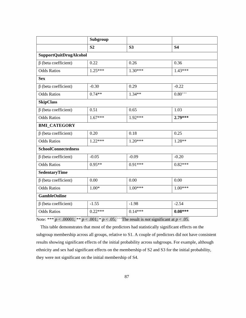
87
Subgroup
S2 S3 S4
SupportQuitDrugAlcohol
β (beta coefficient) 0.22 0.26 0.36
Odds Ratios 1.25*** 1.30*** 1.43***
Sex
β (beta coefficient) -0.30 0.29 -0.22
Odds Ratios 0.74** 1.34** 0.80+++
SkipClass
β (beta coefficient) 0.51 0.65 1.03
Odds Ratios 1.67*** 1.92*** 2.79***
BMI_CATEGORY
β (beta coefficient) 0.20 0.18 0.25
Odds Ratios 1.22*** 1.20*** 1.28**
SchoolConnectedness
β (beta coefficient) -0.05 -0.09 -0.20
Odds Ratios 0.95** 0.91*** 0.82***
SedentaryTime
β (beta coefficient) 0.00 0.00 0.00
Odds Ratios 1.00* 1.00*** 1.00***
GambleOnline
β (beta coefficient) -1.55 -1.98 -2.54
Odds Ratios 0.22*** 0.14*** 0.08***
Note: *** p < .00001; ** p < .001; * p < .05; +++The result is not significant at p < .05.
This table demonstrates that most of the predictors had statistically significant effects on the
subgroup membership across all groups, relative to S1. A couple of predictors did not have consistent
results showing significant effects of the initial probability across subgroups. For example, although
ethnicity and sex had significant effects on the membership of S2 and S3 for the initial probability,
they were not significant on the initial membership of S4.
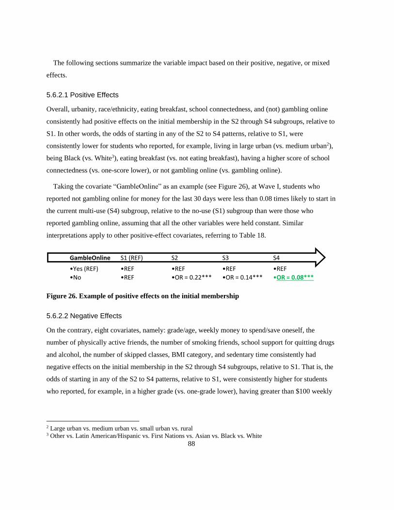
88
The following sections summarize the variable impact based on their positive, negative, or mixed
effects.
5.6.2.1 Positive Effects
Overall, urbanity, race/ethnicity, eating breakfast, school connectedness, and (not) gambling online
consistently had positive effects on the initial membership in the S2 through S4 subgroups, relative to
S1. In other words, the odds of starting in any of the S2 to S4 patterns, relative to S1, were
consistently lower for students who reported, for example, living in large urban (vs. medium urban2),
being Black (vs. White3), eating breakfast (vs. not eating breakfast), having a higher score of school
connectedness (vs. one-score lower), or not gambling online (vs. gambling online).
Taking the covariate “GambleOnline” as an example (see Figure 26), at Wave I, students who
reported not gambling online for money for the last 30 days were less than 0.08 times likely to start in
the current multi-use (S4) subgroup, relative to the no-use (S1) subgroup than were those who
reported gambling online, assuming that all the other variables were held constant. Similar
interpretations apply to other positive-effect covariates, referring to Table 18.
Figure 26. Example of positive effects on the initial membership
5.6.2.2 Negative Effects
On the contrary, eight covariates, namely: grade/age, weekly money to spend/save oneself, the
number of physically active friends, the number of smoking friends, school support for quitting drugs
and alcohol, the number of skipped classes, BMI category, and sedentary time consistently had
negative effects on the initial membership in the S2 through S4 subgroups, relative to S1. That is, the
odds of starting in any of the S2 to S4 patterns, relative to S1, were consistently higher for students
who reported, for example, in a higher grade (vs. one-grade lower), having greater than $100 weekly
2 Large urban vs. medium urban vs. small urban vs. rural 3 Other vs. Latin American/Hispanic vs. First Nations vs. Asian vs. Black vs. White
•REF
•OR = 0.08***
S4
•REF
•OR = 0.14***
S3
•REF
•OR = 0.22***
S2
•REF
•REF
S1 (REF)
•Yes (REF)
•No
GambleOnline

89
money (vs. $21-$1004), five or more physically active friends (vs. 45), five or more smoking friends
(vs. 46), residing in a school very unsupportive (vs. unsupportive7), having more than 20 classes
skipped (vs. 11 to 20 classes8), being obese (vs. overweight9), or having longer sedentary time (vs.
one-minute shorter).
Taking the covariate “SkipClass” as an example (see Figure 27), at Wave I, an individual who
reported skipping 1 or 2 classes was more than 2.79 times likely to start in the current multi-use (S4)
subgroup relative to the no-use (S1) subgroup than was an individual who reported zero skipped
classes, assuming that all the other variables were held constant. The same OR applies to comparing
all the categories, i.e., “zero” vs. “1 or 2 classes” vs. “3 to 5 classes” vs. “6 to 10 classes” vs. “11 to
20 classes” vs. “More than 20 classes.” Similar interpretations hold for other negative-effect
covariates, referring to Table 18.
Figure 27. Example of negative effects on the initial membership
5.6.2.3 Mixed Effects
The covariate sex had mixed negative and positive effects on the initial membership in the S2 through
S4 subgroups relative to S1. The interpretation of this finding can be summarized as follows.
Assuming that all the other variables were held constant, at Wave I, a male student was less than 0.74
times as likely to be in the occasional single-use of alcohol (S2) subgroup relative to the no-use (S1)
subgroup and was less than 0.80 times as likely to be in the current multi-use (S4) subgroup relative
to non-users (S1) subgroup than a female student. Whereas at Wave I, a male student was more than
1.34 times as likely to be in the dual-use of e-cigarette and alcohol (S3) subgroup relative to the no-
use (S1) subgroup than a female student, with all the other variables held constant. Figure 28
4 Greater than $100 vs. $21-$100 vs. $1-$20 vs. zero 5 5 or more friends vs. 4 friends vs. 3 friends vs. 2 friends vs. 1 friend vs. none 6 5 or more friends vs. 4 friends vs. 3 friends vs. 2 friends vs. 1 friend vs. zero 7 Very unsupportive vs. unsupportive vs. supportive vs. very supportive 8 More than 20 classes vs. 11 to 20 classes vs. 6 to 10 classes vs. 3 to 5 classes vs. 1 or 2 classes vs. zero 9 Obese vs. overweight vs. healthy weight vs. underweight vs. not stated
•REF
•OR = 2.79***
S4
•REF
•OR = 1.92***
S3
•REF
•OR = 1.67***
S2
•REF
•REF
S1 (REF)
•Zero (REF)
•1 or 2 classes
SkipClass
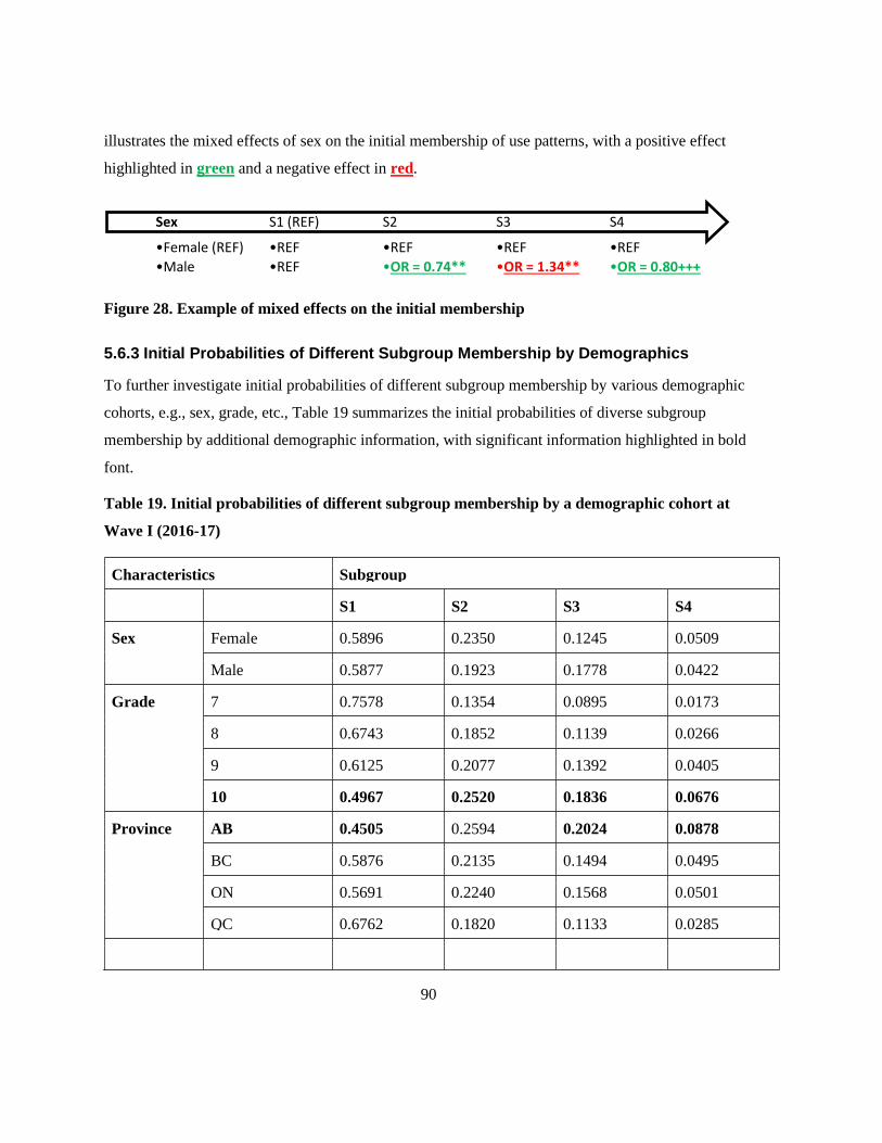
90
illustrates the mixed effects of sex on the initial membership of use patterns, with a positive effect
highlighted in green and a negative effect in red.
Figure 28. Example of mixed effects on the initial membership
5.6.3 Initial Probabilities of Different Subgroup Membership by Demographics
To further investigate initial probabilities of different subgroup membership by various demographic
cohorts, e.g., sex, grade, etc., Table 19 summarizes the initial probabilities of diverse subgroup
membership by additional demographic information, with significant information highlighted in bold
font.
Table 19. Initial probabilities of different subgroup membership by a demographic cohort at
Wave I (2016-17)
Characteristics Subgroup
S1 S2 S3 S4
Sex Female 0.5896 0.2350 0.1245 0.0509
Male 0.5877 0.1923 0.1778 0.0422
Grade 7 0.7578 0.1354 0.0895 0.0173
8 0.6743 0.1852 0.1139 0.0266
9 0.6125 0.2077 0.1392 0.0405
10 0.4967 0.2520 0.1836 0.0676
Province AB 0.4505 0.2594 0.2024 0.0878
BC 0.5876 0.2135 0.1494 0.0495
ON 0.5691 0.2240 0.1568 0.0501
QC 0.6762 0.1820 0.1133 0.0285
•REF
•OR = 0.80+++
S4
•REF
•OR = 1.34**
S3
•REF
•OR = 0.74**
S2
•REF
•REF
S1 (REF)
•Female (REF)
•Male
Sex

91
Characteristics Subgroup
S1 S2 S3 S4
Urbanity Rural 0.2977 0.2734 0.2539 0.1751
Small urban 0.5155 0.2370 0.1811 0.0664
Medium urban 0.5435 0.2335 0.1682 0.0548
Large urban 0.6440 0.1983 0.1245 0.0332
Ethnicity White 0.5828 0.2264 0.1483 0.0426
Black 0.5668 0.2094 0.1698 0.0540
Asian 0.6375 0.1882 0.1327 0.0416
Aboriginal 0.4354 0.1935 0.2253 0.1457
Latin American 0.6129 0.1735 0.1533 0.0603
Other 0.6269 0.1771 0.1406 0.0555
Household
Income
$25K - $50K 0.6845 0.1831 0.1062 0.0262
$50K - $75K 0.5723 0.2184 0.1579 0.0514
$75K - $100K 0.5711 0.2260 0.1536 0.0492
>$100K 0.5548 0.2233 0.1650 0.0568
BMI Not stated 0.6684 0.1651 0.1248 0.0418
Underweight 0.6598 0.1850 0.1214 0.0338
Healthy weight 0.5778 0.2303 0.1481 0.0438
Overweight 0.5030 0.2493 0.1836 0.0641
Obese 0.4540 0.2577 0.2128 0.0755
5.7 Exploring Dynamic Transitions of Youth Polysubstance Use Patterns
5.7.1 How Do Transition Behaviours Change Over Time?
The last primary research question (RQ3) investigated was, “How do transition behaviours change
over time in use patterns?” Transition probabilities were calculated with the LMM modelling to
address this research question. Tables 20-21 show the averaged transition probability matrix across
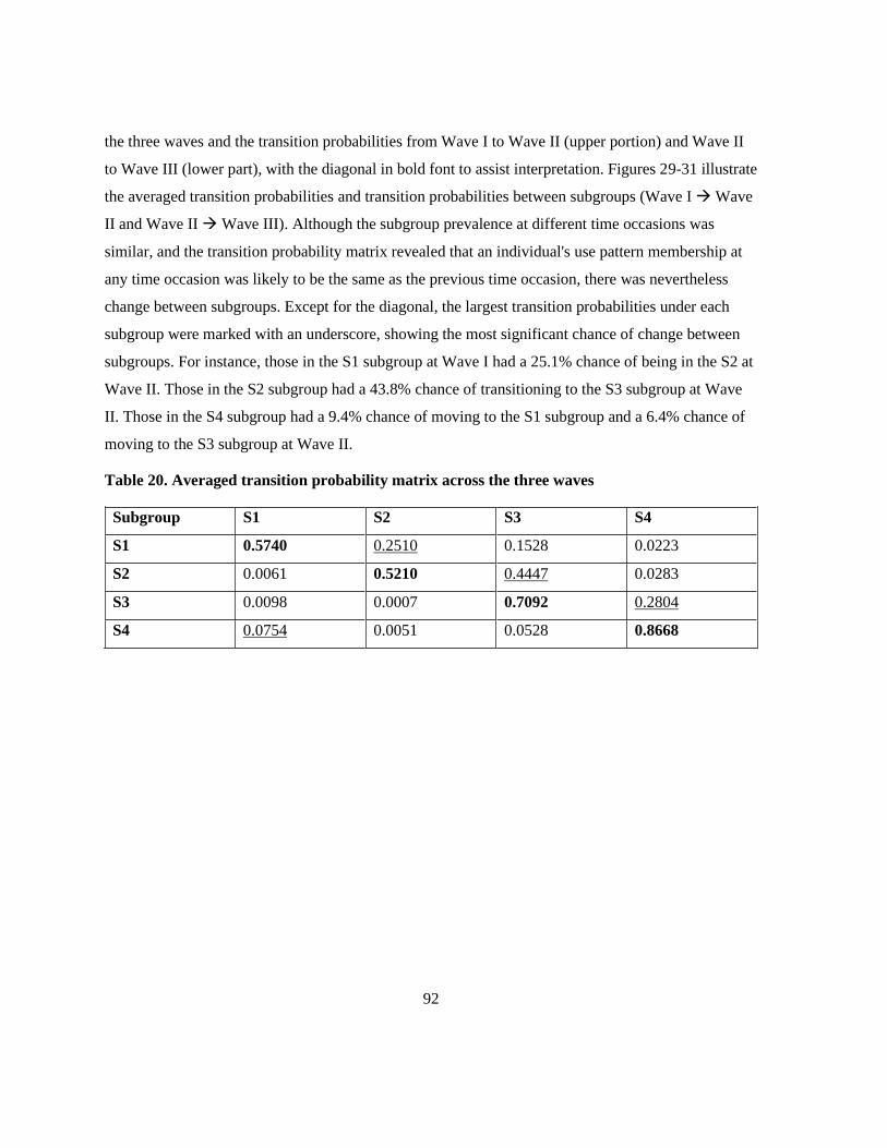
92
the three waves and the transition probabilities from Wave I to Wave II (upper portion) and Wave II
to Wave III (lower part), with the diagonal in bold font to assist interpretation. Figures 29-31 illustrate
the averaged transition probabilities and transition probabilities between subgroups (Wave I → Wave
II and Wave II → Wave III). Although the subgroup prevalence at different time occasions was
similar, and the transition probability matrix revealed that an individual's use pattern membership at
any time occasion was likely to be the same as the previous time occasion, there was nevertheless
change between subgroups. Except for the diagonal, the largest transition probabilities under each
subgroup were marked with an underscore, showing the most significant chance of change between
subgroups. For instance, those in the S1 subgroup at Wave I had a 25.1% chance of being in the S2 at
Wave II. Those in the S2 subgroup had a 43.8% chance of transitioning to the S3 subgroup at Wave
II. Those in the S4 subgroup had a 9.4% chance of moving to the S1 subgroup and a 6.4% chance of
moving to the S3 subgroup at Wave II.
Table 20. Averaged transition probability matrix across the three waves
Subgroup S1 S2 S3 S4
S1 0.5740 0.2510 0.1528 0.0223
S2 0.0061 0.5210 0.4447 0.0283
S3 0.0098 0.0007 0.7092 0.2804
S4 0.0754 0.0051 0.0528 0.8668
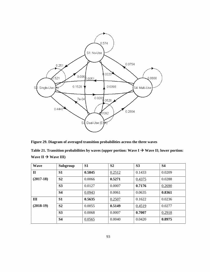
93
Figure 29. Diagram of averaged transition probabilities across the three waves
Table 21. Transition probabilities by waves (upper portion: Wave I → Wave II; lower portion:
Wave II → Wave III)
Wave Subgroup S1 S2 S3 S4
II
(2017-18)
S1 0.5845 0.2512 0.1433 0.0209
S2 0.0066 0.5271 0.4375 0.0288
S3 0.0127 0.0007 0.7176 0.2690
S4 0.0943 0.0061 0.0635 0.8361
III
(2018-19)
S1 0.5635 0.2507 0.1622 0.0236
S2 0.0055 0.5149 0.4519 0.0277
S3 0.0068 0.0007 0.7007 0.2918
S4 0.0565 0.0040 0.0420 0.8975
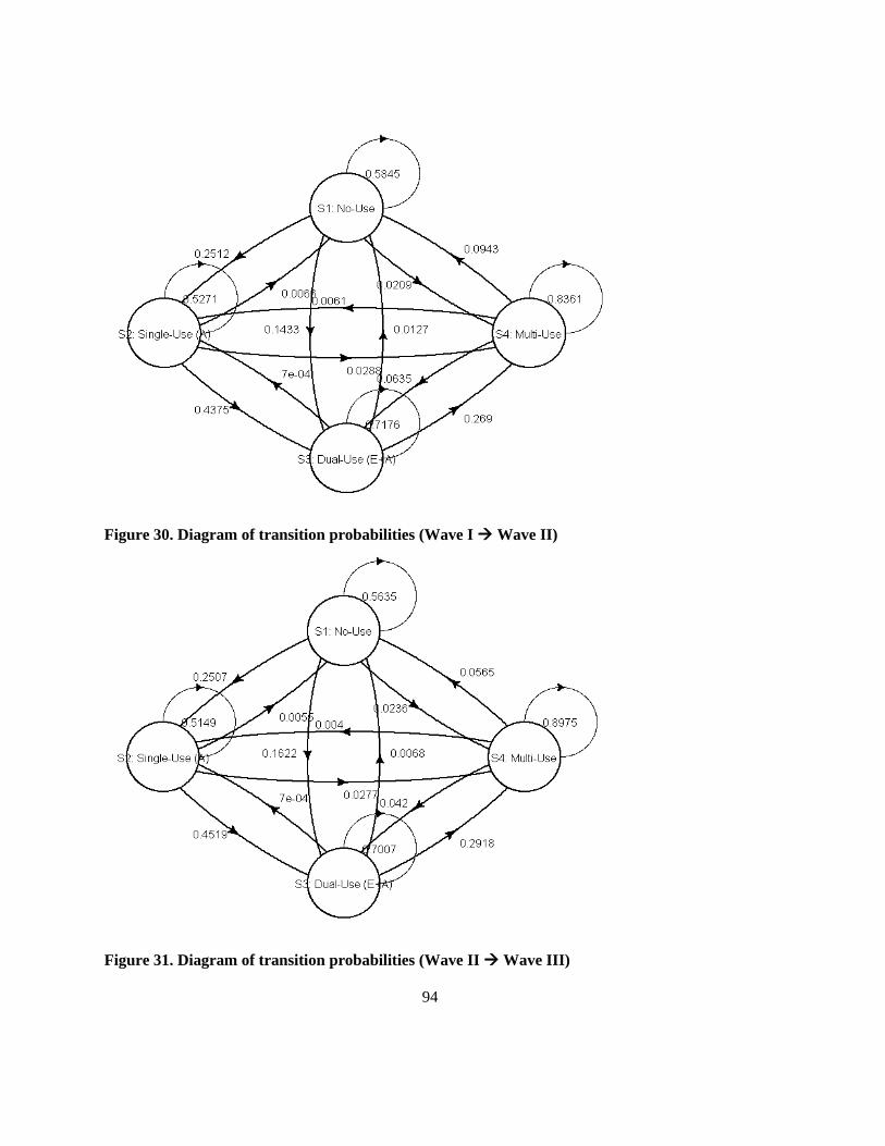
94
Figure 30. Diagram of transition probabilities (Wave I → Wave II)
Figure 31. Diagram of transition probabilities (Wave II → Wave III)
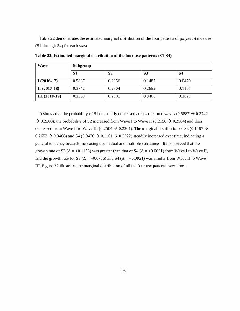
95
Table 22 demonstrates the estimated marginal distribution of the four patterns of polysubstance use
(S1 through S4) for each wave.
Table 22. Estimated marginal distribution of the four use patterns (S1-S4)
Wave Subgroup
S1 S2 S3 S4
I (2016-17) 0.5887 0.2156 0.1487 0.0470
II (2017-18) 0.3742 0.2504 0.2652 0.1101
III (2018-19) 0.2368 0.2201 0.3408 0.2022
It shows that the probability of S1 constantly decreased across the three waves (0.5887 → 0.3742
→ 0.2368); the probability of S2 increased from Wave I to Wave II (0.2156 → 0.2504) and then
decreased from Wave II to Wave III (0.2504 → 0.2201). The marginal distribution of S3 (0.1487 →
0.2652 → 0.3408) and S4 (0.0470 → 0.1101 → 0.2022) steadily increased over time, indicating a
general tendency towards increasing use in dual and multiple substances. It is observed that the
growth rate of S3 (Δ = +0.1156) was greater than that of S4 (Δ = +0.0631) from Wave I to Wave II,
and the growth rate for S3 (Δ = +0.0756) and S4 (Δ = +0.0921) was similar from Wave II to Wave
III. Figure 32 illustrates the marginal distribution of all the four use patterns over time.
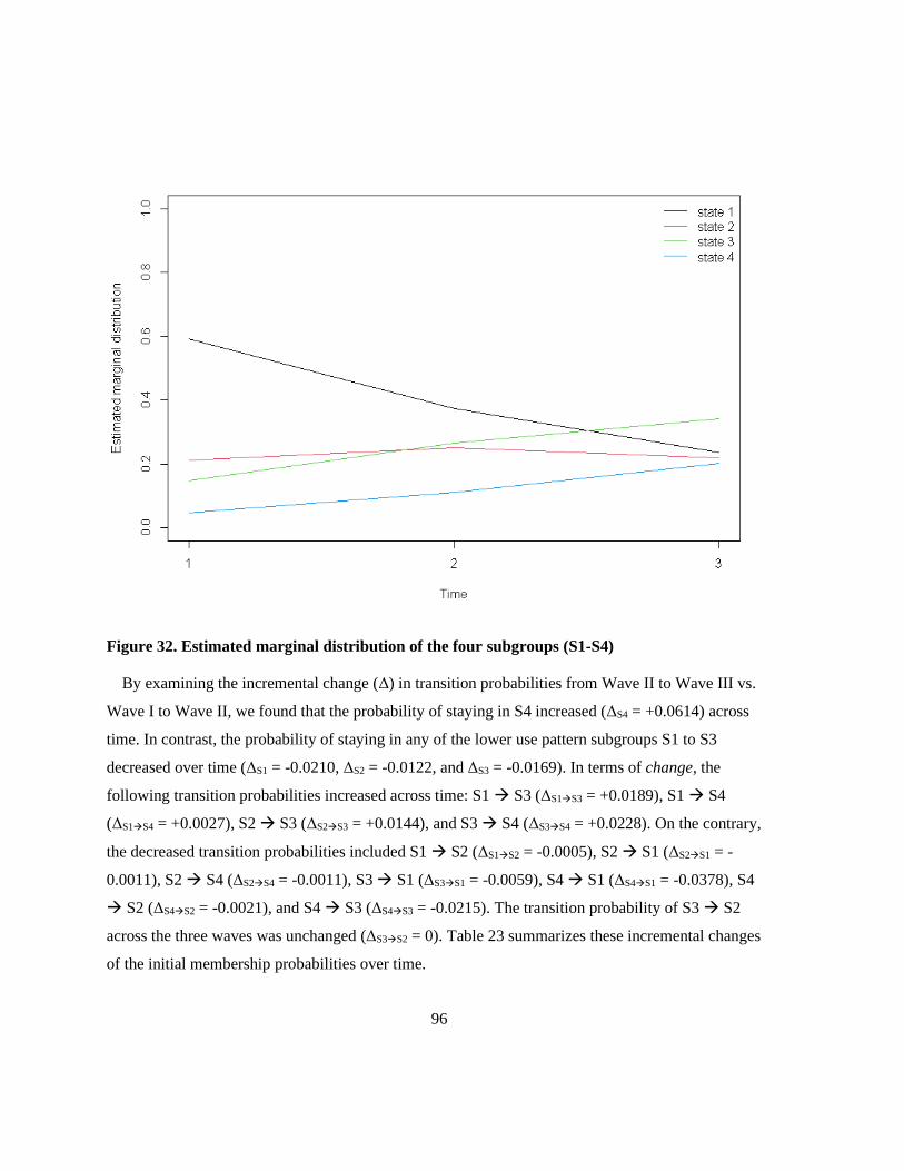
96
Figure 32. Estimated marginal distribution of the four subgroups (S1-S4)
By examining the incremental change (Δ) in transition probabilities from Wave II to Wave III vs.
Wave I to Wave II, we found that the probability of staying in S4 increased (ΔS4 = +0.0614) across
time. In contrast, the probability of staying in any of the lower use pattern subgroups S1 to S3
decreased over time (ΔS1 = -0.0210, ΔS2 = -0.0122, and ΔS3 = -0.0169). In terms of change, the
following transition probabilities increased across time: S1 → S3 (ΔS1→S3 = +0.0189), S1 → S4
(ΔS1→S4 = +0.0027), S2 → S3 (ΔS2→S3 = +0.0144), and S3 → S4 (ΔS3→S4 = +0.0228). On the contrary,
the decreased transition probabilities included S1 → S2 (ΔS1→S2 = -0.0005), S2 → S1 (ΔS2→S1 = -
0.0011), S2 → S4 (ΔS2→S4 = -0.0011), S3 → S1 (ΔS3→S1 = -0.0059), S4 → S1 (ΔS4→S1 = -0.0378), S4
→ S2 (ΔS4→S2 = -0.0021), and S4 → S3 (ΔS4→S3 = -0.0215). The transition probability of S3 → S2
across the three waves was unchanged (ΔS3→S2 = 0). Table 23 summarizes these incremental changes
of the initial membership probabilities over time.

97
Table 23. Incremental change in transition probabilities across the three waves
Δ = PWIIWIII – PWIWII S1 S2 S3 S4
S1 -0.0210 -0.0005 0.0189 0.0027
S2 -0.0011 -0.0122 0.0144 -0.0011
S3 -0.0059 0 -0.0169 0.0228
S4 -0.0378 -0.0021 -0.0215 0.0614
Local decoding is based on the maximum posterior probability. Table 24 presents the prediction of
each subgroup membership at different time occasions. It is noted that the prevalence of S1 through
S4 gradually decreased at Wave II as well, being 38.8%, 24.8%, 24.7%, and 11.7%. A similar trend
was observed in Wave III data, 24.9%, 22.6%, 32.4%, and 20.1%, with the obvious exception in S3,
with the highest prevalence of 32.4%, instead of S1 found with the other two waves. The longitudinal
evidence of use patterns showed that although the no-use (S1) subgroup at Wave I was prominent, its
prevalence decreased over time (Wave I → Wave II: ΔS1 = -21.5%; Wave II → Wave III: ΔS1 = -
13.9%). In contrast, the prevalence of the other three use patterns (S2 to S4) increased (Wave I →
Wave II: ΔS2 = +3.7%, ΔS3 = +10.6%, ΔS4 = +7.2%; Wave II → Wave III: ΔS2 = -2.2%, ΔS3 = +7.7%,
ΔS4 = +8.4%), except for S2 decreased by 2.2% from Wave II to Wave III. By Wave III, S3 became
the prominent use pattern. Although S4 had been the minor use pattern across the three waves, it is
alarming that the prevalence increased by 4.5 times from Wave I to Wave III, and by Wave III, its
prevalence became very close to S2 and S1. The estimated marginal distribution plot and transition
patterns (Figures 32-33 in Chapter 5 Results, Section 5.7.1) depict this trend.
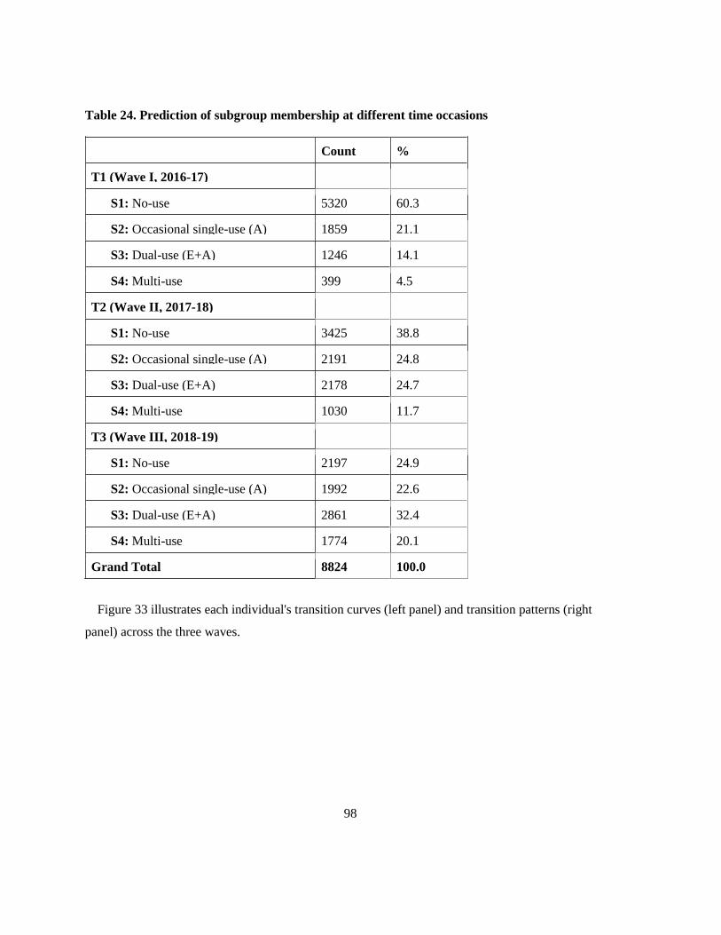
98
Table 24. Prediction of subgroup membership at different time occasions
Count %
T1 (Wave I, 2016-17)
S1: No-use 5320 60.3
S2: Occasional single-use (A) 1859 21.1
S3: Dual-use (E+A) 1246 14.1
S4: Multi-use 399 4.5
T2 (Wave II, 2017-18)
S1: No-use 3425 38.8
S2: Occasional single-use (A) 2191 24.8
S3: Dual-use (E+A) 2178 24.7
S4: Multi-use 1030 11.7
T3 (Wave III, 2018-19)
S1: No-use 2197 24.9
S2: Occasional single-use (A) 1992 22.6
S3: Dual-use (E+A) 2861 32.4
S4: Multi-use 1774 20.1
Grand Total 8824 100.0
Figure 33 illustrates each individual's transition curves (left panel) and transition patterns (right
panel) across the three waves.

99
Figure 33. Transition curves (left panel) and transition patterns (right panel)
5.7.2 What Factors are Associated with Dynamic Transitions of Use Patterns?
One of the secondary research questions (RQ5), in association with the primary research question
RQ3, examined, “What factors are associated with dynamic transitions of use patterns?” Given that
the parameter estimation is cumbersome and the interpretation may be difficult, the ORs for all
covariates of transition between different use patterns are presented in Table 25. This table
demonstrates the average effect of each covariate on the transition probability to the different
subgroups, conditional on the subgroup at Wave I. See Appendix P for detailed covariates' effects on
the transition probabilities with coefficients.
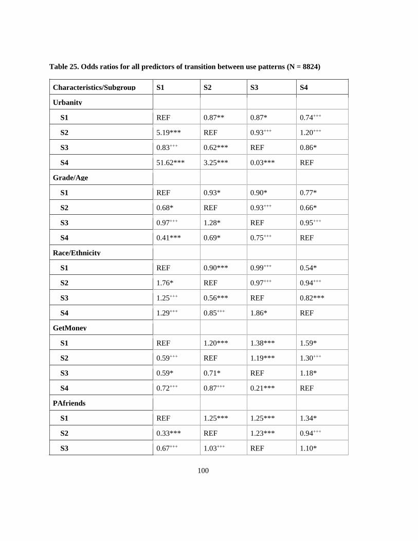
100
Table 25. Odds ratios for all predictors of transition between use patterns (N = 8824)
Characteristics/Subgroup S1 S2 S3 S4
Urbanity
S1 REF 0.87** 0.87* 0.74+++
S2 5.19*** REF 0.93+++ 1.20+++
S3 0.83+++ 0.62*** REF 0.86*
S4 51.62*** 3.25*** 0.03*** REF
Grade/Age
S1 REF 0.93* 0.90* 0.77*
S2 0.68* REF 0.93+++ 0.66*
S3 0.97+++ 1.28* REF 0.95+++
S4 0.41*** 0.69* 0.75+++ REF
Race/Ethnicity
S1 REF 0.90*** 0.99+++ 0.54*
S2 1.76* REF 0.97+++ 0.94+++
S3 1.25+++ 0.56*** REF 0.82***
S4 1.29+++ 0.85+++ 1.86* REF
GetMoney
S1 REF 1.20*** 1.38*** 1.59*
S2 0.59+++ REF 1.19*** 1.30+++
S3 0.59* 0.71* REF 1.18*
S4 0.72+++ 0.87+++ 0.21*** REF
PAfriends
S1 REF 1.25*** 1.25*** 1.34*
S2 0.33*** REF 1.23*** 0.94+++
S3 0.67+++ 1.03+++ REF 1.10*
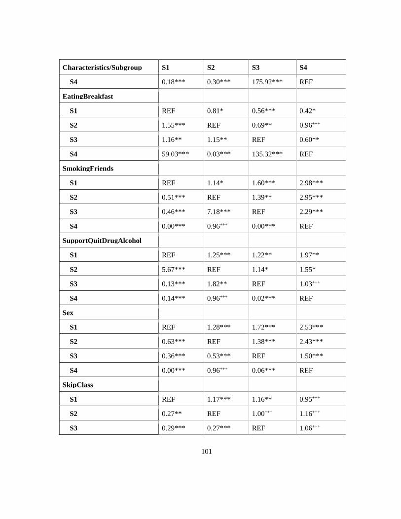
101
Characteristics/Subgroup S1 S2 S3 S4
S4 0.18*** 0.30*** 175.92*** REF
EatingBreakfast
S1 REF 0.81* 0.56*** 0.42*
S2 1.55*** REF 0.69** 0.96+++
S3 1.16** 1.15** REF 0.60**
S4 59.03*** 0.03*** 135.32*** REF
SmokingFriends
S1 REF 1.14* 1.60*** 2.98***
S2 0.51*** REF 1.39** 2.95***
S3 0.46*** 7.18*** REF 2.29***
S4 0.00*** 0.96+++ 0.00*** REF
SupportQuitDrugAlcohol
S1 REF 1.25*** 1.22** 1.97**
S2 5.67*** REF 1.14* 1.55*
S3 0.13*** 1.82** REF 1.03+++
S4 0.14*** 0.96+++ 0.02*** REF
Sex
S1 REF 1.28*** 1.72*** 2.53***
S2 0.63*** REF 1.38*** 2.43***
S3 0.36*** 0.53*** REF 1.50***
S4 0.00*** 0.96+++ 0.06*** REF
SkipClass
S1 REF 1.17*** 1.16** 0.95+++
S2 0.27** REF 1.00+++ 1.16+++
S3 0.29*** 0.27*** REF 1.06+++

102
Characteristics/Subgroup S1 S2 S3 S4
S4 0.71* 0.02*** 98.97*** REF
BMI_CATEGORY
S1 REF 1.02* 0.94** 0.94+++
S2 0.68* REF 1.00+++ 0.88*
S3 1.44** 0.73* REF 0.95*
S4 1.15+++ 1.35* 1.03+++ REF
SchoolConnectedness
S1 REF 0.65*** 1.31* 2.29*
S2 2.26*** REF 1.10+++ 0.18***
S3 1.65*** 1.30*** REF 1.82***
S4 300.22*** 0.05*** 0.46*** REF
SedentaryTime
S1 REF 1.00+++ 1.00*** 1.00*
S2 0.99* REF 1.00** 1.00*
S3 1.00+++ 0.99+++ REF 1.00**
S4 1.00* 1.00+++ 1.01*** REF
GambleOnline
S1 REF 1.37+++ 0.91+++ 0.17***
S2 1.44*** REF 1.32+++ 3.34***
S3 0.72*** 0.70*** REF 1.38+++
S4 0.68*** 1.02+++ 0.00*** REF
Note: *** p < .00001; ** p < .001; * p < .05; +++The result is not significant at p < .05.
Similar to the interpretation of the covariates' effects on initial probabilities, we summarize the
covariates’ effects on the transition probabilities based on their positive, negative, or mixed effects.
This was determined by examining the upper and lower triangular matrices of each covariate in Table
25. Suppose the odds ratios on the upper-triangular matrix were greater than one. In that case, it

103
indicates a higher OR (>1) of transitioning to a higher use pattern, conditional on the reference group
at Wave I. In other words, these factors are more likely to contribute to the dynamic transition to a
higher subgroup. Suppose the odds ratios on the upper-triangular matrix were less than 1. In that case,
it indicates a lower OR (<1) of transitioning to a higher use pattern, conditional on the reference
group at Wave I, suggesting a positive effect on the transition probability to a higher subgroup.
Suppose the ORs on the upper-triangular matrix were mixed with values greater than one and less
than one. In that case, it indicates mixed effects on transition probability to a higher use pattern,
conditional on the reference group at Wave I.
5.7.2.1 Moving From a Lower Use Pattern to a Higher One
5.7.2.1.1 Positive Effects
Overall, grade/age, race/ethnicity, and eating breakfast consistently had positive effects on the
transition probabilities from a lower use pattern to a higher use group over time. Taking the covariate
EatingBreakfast as an example (see Figure 34), among students who started in the no-use subgroup
(S1) at Wave I, those who reported eating breakfast were less than 0.42 times likely to move to the
current multi-use subgroup (S4) relative to S1 at Wave II than were those who reported not eating
breakfast, with all the other variables held constant.
Figure 34. Example of positive effects on the dynamic transitions from a lower use pattern to a
higher one
5.7.2.1.2 Negative Effects
Generally, five covariates, including weekly money to spend/save oneself, the number of smoking
friends, school support for quitting drugs and alcohol, sex (being males), and sedentary time had
consistently negative effects on the dynamic transitions from a lower use pattern to a higher one. For
instance, for the covariate “the number of smoking friends” (see Figure 35), with all the other
•OR = 0.42*
•OR = 0.96+++
•OR = 0.60**
•REF
S4
•OR = 0.56***
•OR = 0.69**
•REF
S3
•OR = 0.81*
•REF
S2
•REF
S1
•S1
•S2
•S3
•S4
Eating breakfastNo (REF)Yes

104
variables held constant, among students who started in the no-use subgroup (S1) at Wave I, those who
reported having one smoking friend were more than 2.98 times likely to transition to the current
multi-use subgroup (S4) in relation to S1 at Wave II than were those who reported zero friends who
smoke. The same OR applies to “None” vs. “1 friend” vs. “2 friends” vs. “3 friends” vs. “4 friends”
vs. “5 or more friends.”
Figure 35. Example of negative effects on the dynamic transitions from a lower use pattern to a
higher one
5.7.2.1.3 Mixed Effects
More covariates had mixed effects on transition probabilities than on initial probabilities. The
variables with inconsistent effects on the transition probabilities from a lower use pattern to a higher
one include urbanity, the number of physically active friends, the number of skipped classes, BMI
category, school connectedness, and gamble online. Taking the GambleOnline effect as an example,
with all the other variables held constant, among students who started in the single-use of alcohol
subgroup (S2) at Wave I, those who reported not gambling online for money for the last 30 days were
more than 3.34 times likely to move to the multi-use subgroup (S4) in relation to S2 at Wave II than
were those who reported gambling online. Whereas among students who started in the no-use
subgroup (S1) at Wave I, those who reported not gambling online for money for the last 30 days were
less than 0.17 times likely to transition to the current multi-use subgroup (S4) in relation to S1 at
Wave II than were those who reported gamble online. Figure 36 demonstrates the mixed effects of
GambleOnline on the dynamic transitions from a lower use pattern to a higher one, with a positive
effect highlighted in green and a negative effect in red.
•OR = 2.98***
•OR = 2.95***
•OR = 2.29***
•REF
S4
•OR = 1.60***
•OR = 1.39**
•REF
S3
•OR = 1.14*
•REF
S2
•REF
S1
•S1
•S2
•S3
•S4
SmokingFriendsZero (REF)1 friend

105
Figure 36. Example of mixed effects on the dynamic transitions from a lower use pattern to a
higher one
5.7.2.2 Moving from a Higher Use Pattern to a Lower One
Likewise, the odds ratios on the lower-triangular matrix indicate the effects on transition probability
from a higher use pattern to a lower one, conditional on the reference group at Wave I. A summary of
the variables and their effects follows, based on the lower-triangular matrix presented in Table 25.
5.7.2.2.1 Negative Effects
Only two covariates, weekly money to spend/save oneself and sex, consistently affected the transition
probabilities from a higher use pattern to a lower one in a negative way. Being males or having more
weekly money was associated with an increased risk of dynamic transitioning from a higher use
pattern to a lower one over time. For instance, among students who started in the dual-use of e-
cigarette and alcohol subgroup (S3) at Wave I, male students were less than 0.36 times as likely to
transition to the no-use subgroup (S1) in relation to S3 at Wave II than were female students, with all
the other variables held constant. Figure 37 demonstrates the negative effects of gender on the
dynamic transitions from a higher use pattern to a lower one.
Figure 37. Example of negative effects on the dynamic transitions from a higher use pattern to a
lower one
•OR = 0.17***
•OR = 3.34***
•OR = 1.38+++
•REF
S4
•OR = 0.91+++
•OR = 1.32+++
•REF
S3
•OR = 1.37+++
•REF
S2
•REF
S1
•S1
•S2
•S3
•S4
GambleOnlineYes (REF)No
•REF
S4
•REF
•OR = 0.06***
S3
•REF
•OR = 0.53***
•OR = 0.96+++
S2
•REF
•OR = 0.63***
•OR = 0.36***
•OR = 0.00***
S1
•S1
•S2
•S3
•S4
SexFemale (REF)Male

106
5.7.2.2.2 Mixed Effects
More covariates had inconsistent effects on the transition probabilities from a higher use pattern to a
lower one. These variables are urbanity, grade/age, race/ethnicity, the number of physically active
friends, eating breakfast, the number of smoking friends, school support for quitting drugs and
alcohol, the number of skipped classes, BMI category, school connectedness, sedentary time, and
gamble online. For example, with all the other variables held constant, among students who started in
the single-use of alcohol subgroup (S2) at Wave I, those who reported not gambling online were more
than 1.44 times as likely to transition to the no-use subgroup (S1) in relation to S2 at Wave II than
were those who reported gamble online. However, among students who started in the current multi-
use subgroup (S4) at Wave I, those who reported not gambling online were less than 0.68 times as
likely to transition to the no-use subgroup (S1) in relation to S4 at Wave II than were those who
reported gamble online. Figure 38 shows the mixed effects of GambleOnline on the dynamic
transitions from a higher use pattern to a lower one, with a positive effect highlighted in green and a
negative effect in red.
Figure 38. Example of mixed effects on the dynamic transitions from a higher use pattern to a
lower one
In summary, this chapter reported the study results, starting from MI for missing values, descriptive
statistics, factors associated with youth polysubstance use, risk profiles phenotypes, and the dynamic
transitions of polysubstance use patterns among youth. The next chapter will discuss the key findings
from public health and ML methodological perspectives, the contributions to the practice and the
literature, strengths and limitations of this thesis, and future research directions.
•REF
S4
•REF
•OR = 0.00***
S3
•REF
•OR = 0.70***
•OR = 1.02+++
S2
•REF
•OR = 1.44***
•OR = 0.72***
•OR = 0.68***
S1
•S1
•S2
•S3
•S4
GambleOnlineYes (REF)No

107
Chapter 6
Discussion
This chapter discusses the key findings of this thesis, including the main results of risk profiling,
patterns of polysubstance use among youths, and the dynamic transitions of these use patterns over
time. The perceptions from a methodological perspective, particularly the selection and appropriate
application of ML methods modelling risk profiles and dynamic transitions using the COMPASS
data, ML interpretability and fairness, and data infrastructure and capacity that enables ML, are also
discussed. Finally, the contributions of this thesis to public health practitioners and the research
communities, the strengths and limitations, and future works are presented in this chapter.
6.1 Key Findings
6.1.1 Phenotyping Risk Profiles of Youth Polysubstance Use
6.1.1.1 Overview of the Risk Profiles and Associated Factors
One of the primary research questions (RQ1) of this thesis was, “What are the risk profiles of
polysubstance use among Canadian secondary school students?” Before examining the risk profiles,
we first identified the top eight factors associated with youth polysubstance use. Ranked by the
variable importance, these factors include the number of smoking friends, the number of skipped
classes, weekly money to spend/save oneself, sedentary time, CESD, school connectedness, eating
breakfast, and grade (as a proxy of age). These factors are consistent with the findings in the
literature. Some of the risk factors that correlate with polysubstance use among youth included age,
sex, ethnicity, eating habits, PA and sedentary behaviour, social connectedness, and family and peer
influence (see Chapter 2 Literature Review, Section 2.1.3). Although some studies reported that sex
and race/ethnicity play an important role in youth polysubstance use (13,14,40,41), these two were
not ranked as top features in the COMPASS data. Therefore, we did not include them for phenotyping
risk profiles.
The four risk profiles of polysubstance use among Canadian youth identified in this thesis were low
risk (L1), medium-low risk (L2), medium-high risk (L3), and high risk (L4), based on the three
annual waves of the linked samples from the COMPASS datasets analyzed. This was achieved by

108
utilizing the top eight factors correlated with polysubstance use and the four substance use indicators,
i.e., cigarette smoking, e-cigarette use, alcohol drinking, and marijuana consumption. Numerous
studies in addiction research have examined the risk factors associated with polysubstance use among
youth or have identified use patterns. To our knowledge, no literature thus far has ever taken such a
holistic approach to explore risk profiles among youth. Although no direct comparisons between our
results and other studies can be performed, this thesis sheds light on the phenotyping risk profiles of
youth polysubstance use with cross-sectional and longitudinal evidence. The four profiles identified
in this thesis provide a more comprehensive overview of the prominent characteristics for each of the
different risk levels of engaging in polysubstance use among this cohort.
The following section discusses the heterogeneity in the prevalence and phenotype across these
four risk profiles. The numbers presented in the next section represent the group average across the
risk profiles unless otherwise stated.
6.1.1.2 Heterogeneity in Risk Profile Phenotypes
Overall, at Wave I, the majority of students (32.5%) were at low risk (L1), closely followed by L2
(31.5%) and then L3 (24.5%). Only about a tenth of students belonged to the high-risk (L4) profile
for Wave 1, accounting for 11.5% of the total sample size (N = 8610), which equates to
approximately one-third of the low-risk population for all three waves. This trend is observed across
all three waves, except for Wave II, where a slightly higher percentage (35.4%) of students were at
medium-low risk (L2) than those at low risk (L1, 34.7%) (see Tables 13-15 in Chapter 5 Results,
Section 5.5.2). By examining the longitudinal prevalence across the three waves, we found that over
time, the number of students at low risk (L1) increased (from Wave I to Wave III: 32.5% → 34.7% →
38.9%). In contrast, the number of students decreased at both the medium-high risk (L3, from Wave I
to Wave III: 24.5% → 22.0% → 20.4% ) and the high-risk group (L4, from Wave I to Wave III:
11.5% → 7.9% → 7.9%), over time. Interestingly, the prevalence of students at medium-low risk
(L2) increased from Wave I to Wave II (31.5% → 35.4%) and decreased from Wave II to Wave III
(35.4% → 32.7%).
In general, our findings reveal that students who belonged to the low-risk (L1) profile group, on
average, had the lowest mean values (scores) for substance use, CESD, and sedentary time. They also
had, on average, fewest smoking friends, fewest skipped classes, highest mean scores of school
connectedness, and reported eating breakfast. On the contrary, those who belonged to the high-risk

109
group (L4), on average, had the highest mean values (scores) for substance use, CESD, and sedentary
time. And in contrast to L1, they tended to have the highest number of smoking friends, the highest
number of skipped classes, the lowest mean scores of school connectedness, and on average, reported
not eating breakfast. Additionally, two intermediate risk profiles were identified between L1 and L4:
the medium-low risk (L2) and the medium-high risk (L3) group. It is observed that similar trends of
risk profiling appear throughout the three waves, showing consistent risk profiles over time, including
the four substance use indicators and the top factors associated with youth polysubstance use.
It is observed that alcohol was the most prevalent substance used by Canadian youth, followed by
e-cigarettes. Cigarette and marijuana shared a similar prevalence at Wave I across the four risk
profiles. However, the prevalence of marijuana consumption increased more rapidly than that of
cigarette smoking over time.
Based on the Boruta algorithm of variable importance ranking, the top 3 features that affect youth
polysubstance use are unrelated to demographic information like age or sex. Instead, “the number of
smoking friends,” “the number of skipped classes,” and “weekly money to spend/save oneself”
ranked top 3 across the three waves. The first two features reflect peer influence and risky behaviour.
The risk profiling indicates that peer influence has more impact on polysubstance use among youth
than any other identified risk factors.
By investigating the cross-sectional evidence on other included factors, this thesis reveals that a
sedentary lifestyle was associated with high risk of polysubstance use. Our finding agrees with West
et al. (2020) that sedentary behaviour was positively related to adolescent drinking and marijuana
consumption (130). Existing research indicates that sedentary behaviour might be a determinant for
adolescent alcohol and marijuana consumption (130). The same trend was observed for Wave II and
Wave III. Comparing L4 vs. L1 for the last two waves, the sedentary time differences were similar to
Wave I, 6.09 times (1176/193) for Wave II and 5.70 times (1191/209) for Wave III. Similar to the top
3 factors, the magnitudes of sedentary time across the four risk groups (Wave III vs. Wave I) range
from 1.16 times (L3) to 1.23 times (L1) over time.
Students in the high-risk group (L4) had a lower mental health status, which was indicated by the
largest CESD scores. That is, the higher the CESD scores, the more significant the depressive
symptoms that were reported. According to Radloff (1977), a CESD score ≥ 10 indicates clinically
relevant depressive symptoms (131). In Wave I data, students in the L4 group had a CESD score of

110
10.8 ± 6.70, indicating that, on average, this group of individuals already experienced clinically
relevant depressive symptoms. In contrast, those in the low-risk group (L1) had the smallest CESD
score of 7.08 ± 5.39. Subsequently, the medium-low (L2) and medium-high (L3) risk groups had
average CESD scores of 8.34 ± 5.89 and 9.30 ± 6.04, respectively, with significant differences
between each risk group. The same trend was observed in Wave II and III data. This agrees with
Halladay et al. (2020), which also found an association between substance use and mental health.
Many studies have found that individuals in the multi-use group report higher psychiatric symptoms,
including depression and anxiety, than the single-use group (49,50). In a systematic review by Cairns
et al. (2014), the authors identified polysubstance use as a modifiable risk factor for depression
among youth (132).
Comparing across the four risk profiles L1 through L4 (Wave III vs. Wave I), the magnitudes of
the CESD score were similar, 1.13 times (L1), 1.10 times (L2), 1.08 times (L3), and 1.13 times (L4),
implying that the incremental rates for the CESD score were consistent across the four risk patterns
over time. As previously discussed, students in the high-risk group (L4) already experienced
clinically relevant depressive symptoms at Wave I and throughout Wave III due to the increasing
CESD scores over time. It was noted that, on average, individuals in the L3 risk group started to have
clinically relevant depressive symptoms at Wave III.
In addition, this thesis identified good nutritional habits, such as eating breakfast, were associated
with the low risk of polysubstance use among Canadian youth. For example, at Wave I, the majority
(65.4%) of the students in the low-risk group (L1) ate breakfast, while only 31.9% of the students in
the high-risk group (L4) ate breakfast. The prevalence of eating breakfast decreased while the risk
level increased from low-risk (65.4%), medium-low (51.6%), medium-high (42.4%), to high-risk
(31.9%). This similar pattern can be seen throughout the three waves, as shown in Tables 13-15. Our
finding is consistent with the literature about youth polysubstance use and the correlation of nutrition-
related attitudes. For example, Isralowitz and Trostler (1996) reported that substance users were more
likely to be at greater risk of poor eating habits, including not eating breakfast or not eating three
meals daily (52).
The longitudinal evidence of the risk profiles concerning the four substance use indicators showed
that, in general, the scores of these indicators increased across the three waves, indicating that with
time, students engaged to higher use of each substance across the risk profiles (L1 through L4). Note

111
that the incremental rate of marijuana consumption in the low risk (L1) group from Wave I to Wave
III was the largest (6.17) among the four substances, followed by e-cigarette use (4.71), cigarette
smoking (3.5), and alcohol drinking (1.64). Comparing the incremental rates of the score of substance
use indicators across the four risk profiles, the low-risk group had the most significant increase,
followed by L2, L3, and L4, subsequently.
Lastly, using students’ grade level as a proxy of their age, this thesis identified that age was one of
the top factors associated with youth polysubstance use. Among the four risk profiles identified, the
high-risk group comprises mainly older students, while most low-risk groups were their younger
peers. For example, within the low-risk group (L1) at Wave I, 23.9% of students were in grades 7/8
and 26.9% in grade 10. In the high-risk group (L4) at the same wave, only 7.8% of students were in
grades 7/ 8, and 42.9% were in grade 10. A similar pattern was observed at Wave II and III (see
Tables 13-15 in Chapter 5 Results, Section 5.5.2). This finding concurs with published literature that
the age of adolescents directly correlates with increased risk of using substances
(13,32,41,44,46,133,134), i.e., the older the youth, the higher the likelihood of using substances.
6.1.2 Patterns of Polysubstance Use Among Canadian Secondary School Students
6.1.2.1 What are the Polysubstance Use Patterns?
Another primary research question (RQ2) investigated in this thesis was, “What are the patterns of
polysubstance use among Canadian secondary school students?” We identified four distinctive
polysubstance use patterns among youth, which were no-use (S1), occasional single-use of alcohol
(S2), dual-use of e-cigarette and alcohol (S3), and current multi-use (S4). Each use pattern represents
a mutually exclusive overarching theme. The patterns identified suggest an increasing tendency and
frequency of polysubstance use with decreasing membership size with higher risk groups, and each
use pattern has considerably different sizes.
Most studies on polysubstance use among youth focus primarily on tobacco, alcohol, and
marijuana use due to the high prevalence of use in this cohort (67). E-cigarettes have not been
considered in many of these studies due to their novelty. However, the popularity of e-cigarette use
has surged among youth in recent years; it may now be a significant contributing factor to the rise in
youth polysubstance use (13,14). Morean et al. (2016) examined the co-use of multiple substances
such as tobacco products, e-cigarettes, alcohol, and marijuana among high school students in
112
Connecticut, US (133). They identified four classes of use: abstainers (82% of the sample), alcohol
and e-cigarette users (5%), cannabis and alcohol users (7%), and users of all products (7%) (133).
Recent research identifies use patterns that involve dual- and multi-use of e-cigarettes with other
substances, indicating the importance of considering these devices when examining multiple
substance use (133).
In the existing literature on youth polysubstance use utilizing LCA, most studies have identified
three or four patterns of polysubstance use (32). Typical patterns include no or low use, alcohol use
(i.e., alcohol only or predominantly alcohol use), and polysubstance use (32). In a systematic review
of substance use patterns among youth, Halladay et al. (2020) highlighted an average of four use
patterns, including low use, one- or dual-use, moderate multi-use, and high multi-use (67). Their
results have been drawn from 70 individual studies and 89 cluster solutions. Before model
enumeration, the minimum and maximum users are two and six, respectively (67). Our research has
identified four use patterns, which align with the findings by Halladay et al. (2020).
6.1.2.2 What Factors are Associated with Patterns of Polysubstance Use?
One of the secondary research questions (RQ4) examined in this thesis was, “What factors are
associated with patterns of polysubstance use among Canadian adolescents?” Existing evidence
suggests that the factors impacting youth polysubstance use patterns include gender, race, early onset
of alcohol drinking, academic achievements in secondary school, and friendship goals (135).
According to Lanza, Patrick & Maggs (2010), examining alcohol, cigarette, and marijuana use, males
were 4.5 times more likely to be in the highest use group (“bingers with marijuana use”) than their
female counterparts, in comparison to non-users (135). However, with non-users being the reference,
in contrast, females were more prone to smoking cigarettes (OR = 1/0.6) or binge drinking (OR =
1/0.9) than their male counterparts (135). Their findings were consistent with the results of this thesis
concerning the mixed effects of gender on polysubstance use membership among youth. Yet, the
gender difference between the study results by Lanza, Patrick & Maggs (2010) and ours was
inconsistent.
In this thesis, the gender of the cohort had mixed effects on the initial probabilities for different use
patterns. In particular, we found that males were 1.34 times more likely to start in the dual-use of e-
cigarette and alcohol subgroup (S3) than females, relative to the no-use subgroup (S1). In contrast, at
Wave I, females were 1.35 times more likely to engage in occasional single-use of alcohol (S2) and

113
1.25 times more likely to experience current multi-use (S4), the highest use group in this thesis than
their male peers, relative to S1. Except for the implication that female students tend to be more likely
to engage in alcohol intake than their male counterparts, the disparity in gender differences between
our findings and those by Lanza, Patrick & Maggs (2010) could be due to the differences between
substance use indicators and the corresponding measurements assigned. For instance, this thesis
included e-cigarette as an emerging substance, whereas Lanza, Patrick & Maggs (2010) did not.
Additionally, this thesis did not differentiate between regular drinking and binge drinking for alcohol
use, as was it done by Lanza, Patrick & Maggs (2010). Some other differences include the method of
data collection and the age of the population. Lanza, Patrick & Maggs (2010) used data collected at
baseline and 14-days follow-ups in Fall 2007 and Spring 2008 among first-year college students
(135). In comparison, our three waves data were collected from 2016-2017 among secondary school
students. As such, a difference in nearly a decade in data collection and a study population age and
level of education difference between the two studies cannot be neglected as contributing to the
difference in findings.
There is inadequate literature about factors that impact the initial membership of polysubstance use
patterns among youth. Regarding race/ethnicity contributing to polysubstance use membership among
youth, Lanza, Patrick & Maggs (2010) identified that Hispanic Americans were 1.5 times more likely
to be cigarette smokers or “bingers with marijuana use” than European Americans, relative to non-
users. African Americans and Asian Americans were less likely to engage in substance use than
European Americans relative to non-users (135). Our results showed that Black students were 0.92
times less likely to engage in the single-use subgroup (S2) than their White peers, relative to non-
users (S1). Concerning the no-use subgroup (S1), the odds ratios to start in the dual-use (S3) and
current multi-use pattern (S4) for Black vs. White were 0.94 and 0.96, respectively. The study results
indicate that Black students were less likely to engage in a higher use group than their White peers,
same as Black vs. Asian, Asian vs. First Nations, First Nations vs. Latin American/Hispanic, and
Latin American/Hispanic vs. Other. However, the effect was not statistically significant for S4 vs. S1.
In addition to the gender difference and race/ethnicity, what brings new insights into the literature
on the patterns of youth polysubstance use in this thesis is the multifaceted covariates and their effects
that we examined. Within the limited evidence, no other studies included all the variables investigated
in this thesis to evaluate the impact on the initial membership of use patterns, summarized based on

114
their positive, negative, or mixed effects. One should be cautious about interpreting the BMI effect on
the initial membership. The missing values were coded as one category instead of performing
multiple imputations as other missing data. However, the results show that the BMI category did
impact the initial probabilities of the use pattern membership. Generally, the higher the BMI (i.e., not
stated vs. underweight vs. healthy weight vs. overweight vs. obese), the more likely the individual
started in a higher use pattern at Wave I.
It is observed that students who reported, for example, at lower grade levels (e.g., grades 7 or 8),
residing in Quebec, living in large urban settings in Canada, from a household income level between
$25K and $50K, or being underweight according to their BMI, tended to belong to the no-use (S1)
subgroup. Additionally, students with these characteristics generally had a lower chance of being at
the other three higher use groups (S2 to S4) than non-users (S1) at Wave I. In contrast, at Wave I,
students with the highest grade (grade 10), residing in Alberta, from rural areas across Canada, self-
identified as Indigenous, or being obese according to their BMI had a higher chance of belonging to
one of the higher use groups (S2 to S4) and a lower chance of being in the no-use (S1) subgroup.
6.1.3 Exploring Dynamic Transitions of Youth Polysubstance Use Patterns
6.1.3.1 How Do Transition Behaviours Change Over Time?
One of the primary research questions (RQ3) explored in this thesis was, “How do transition
behaviours change over time according to use patterns analysis?” The LMM applied for this thesis
allowed us to investigate the dynamics of polysubstance use patterns among youth. In general, the
resulting transition probabilities provide us with two aspects of the dynamics across time, i.e.,
stability (a subject stays in the same subgroup) and change (transitions to another subgroup). This
section discusses our findings surrounding these two perspectives.
6.1.3.1.1 Stability
Our results revealed that generally, students remained in the same use pattern subgroup across time.
On average, across the three waves, the probabilities for students staying in the no-use (S1), single-
use (S2), dual-use (S3), and multi-use (S4) subgroup were 0.5740, 0.5210, 0.7092, and 0.8668,
respectively. The current multi-use (S4) was the most stable use pattern, followed by the dual-use
(S3) and the no-use (S1) pattern. Among these four patterns, occasional single-use of alcohol (S2)

115
was the least stable pattern, with the probability of remaining in this subgroup across time was the
lowest (0.5210). When they transitioned, it was typically to a higher use pattern adjacent to their
current subgroup (i.e., S1 → S2, S2 → S3, or S3 → S4), rather than to a lower one, except for the
highest use group S4. This finding is consistent with current literature that examines adolescent
polysubstance use with LTA. The evidence suggests that youth are most likely to remain in the same
subgroup of use pattern or transition to a higher use group as they grow older (134,136).
A similar trend was observed by investigating the longitudinal evidence of the transition patterns,
i.e., Wave I → Wave II and Wave II → Wave III. In particular, from Wave I to Wave II, probabilities
for students staying in the no-use (S1), single-use (S2), dual-use (S3), and multi-use (S4) subgroup
were 0.5845, 0.5271, 0.7176, and 0.8361, respectively. From Wave II to Wave III, the probabilities
were 0.5635, 0.5149, 0.7007, and 0.8975 for remaining in the S1, S2, S3, and S4 subgroup. It is
observed that the chance of staying in S4 from Wave II to Wave III was higher (Δ = +0.0614) than
that of from Wave I to Wave II, meaning that with time, current multi-users were more likely than the
last time occasion to stay in this highest use pattern subgroup. While for the other three use patterns
(S1 through S3), the stability decreased over time (ΔS1 = -0.0210; ΔS2 = -0.0122; and ΔS3 = -0.0169).
The decreased stability implies that students starting at any of these use patterns had an increased
chance of transitioning to other use patterns across time.
6.1.3.1.2 Change
Table 20 highlights the changing pattern, with underscores indicating the largest transition
probabilities within each subgroup. For example, on average of the two transitions (i.e., Wave I →
Wave II and Wave II → Wave III), for students in the S2 subgroup, the chance of moving to S3 was
0.4447, the largest probability representing the change of use patterns across the three waves. The
second-largest transition probability was S3 → S4 (0.2804), followed by S1 → S2 (0.2510). In
contrast, students in the S3 subgroup were least likely to transition to S2, with the slimmest chance of
0.0007. Similarly, students in the S4 subgroup were unlikely to move to S2 across time, with the
transition probability being 0.0051. In addition, those in S2 or S3 subgroups were less likely to
transition to the S1 subgroup, with small transition probabilities for S2 → S1 (0.0061) and S3 → S1
(0.0098).
Similar to the longitudinal observation of the transition probabilities for stability, we examined the
incremental change in transition probabilities, comparing Wave II → Wave III vs. Wave I → Wave
116
II. Concerning change, in general, the chances of transitioning from a lower use pattern to a higher
one increased over time. This was determined by the increased transition probabilities across time
(positive Δ in Table 23 in Chapter 5 Results, Section 5.7.1). On the contrary, the decreased transition
probabilities (negative Δ in Table 23) indicate slimmer chances of moving from a higher use pattern
to a lower one with time. There were two exceptions, moving from S1 to S2 and S2 to S4, with
decreased probabilities of 0.0005 and 0.0011, respectively.
Note that the measurement interval of cigarette and e-cigarette smoking was the last 30 days,
whereas the measurement interval of alcohol and marijuana use was past year. Many transitions may
have occurred between when student participants were asked about cigarette or e-cigarette smoking in
the last 30 days at Wave I and when they were asked again one year later. It is impossible to estimate
how much movement between subgroups has occurred between these measurement windows for
these two specific substances. In this case, the upper bound of the diagonal elements and the lower
bound of the off-diagonal elements of the transition matrix were used to explain the transition
probabilities (68). Although the lower bound of the off-diagonal elements tends to underestimate
transition over time, the general transition pattern is consistent, as previously discussed.
It is worth noting that not only do use patterns change with time but so does the evidence in use
patterns. For example, with the emerging trend of e-cigarette use among youth, adding e-cigarette as
new evidence while examining use patterns would be more meaningful than ever. Unfortunately, no
prior research examined the dynamic transitions of polysubstance use patterns among youth include
the e-cigarette as a substance use indicator. It contributes to one of the novelties to this thesis. In the
meantime, it makes the direct comparison between our findings and others impossible.
6.1.3.2 What Factors are Associated with Dynamic Transitions of Use Patterns?
One of the secondary research questions (RQ5) explored was, “What factors are associated with
dynamic transitions of use patterns?” Choi et al. (2018) reported that males were more likely to
transition from using legal to more illicit substances than females, while female polysubstance users
were more likely to transition to a less use pattern than males (131,135). Although we did not
examine licit vs. illicit substances in this thesis, the finding is consistent with our results. Our finding
of the gender difference on the dynamic transition of use patterns indicates that male students were
more likely to transition to a higher use group and were less likely to transition to a lower one than
their female peers over time. For example, among students who started in the no-use subgroup (S1) at

117
Wave I, males were 2.53 times more likely to transition to the current multi-use subgroup (S4) at
Wave II than were female students. Whereas transitioning from a higher use pattern to a lower one,
among students who started in the current multi-use subgroup (S4), females were 16.67 times more
likely to move to the dual-use subgroup (S3) relative to S4 at Wave II than were males.
Except for the gender difference, there is inadequate literature about what other variables lead to
the dynamic transitions of membership. Thanks to the rich longitudinal evidence available in the
COMPASS data, we examined multifaceted covariates to determine if they were significant in
predicting the subgroup membership at baseline (Wave I) as discussed in Section 6.1.2.2 or predicting
the dynamic transitions of use patterns over time. These covariates range from demographic
information to health behaviours, from individual-level to population-level (environmental).
Ultimately, our study results provide new insights into what characteristics lead to the dynamic
transitions of youth polysubstance use patterns, summarizing in two directions, i.e., moving from a
lower use pattern to a higher one or the other way around.
On the bright side, students in a higher grade (grade 10 vs. grade 9 vs. grade 8 vs. grade 7), being
Black (vs. White10), or eating breakfast were less likely to transition from a lower use pattern to a
higher one. Among these covariates, eating breakfast had a statistically significant effect on the
dynamic transition of use pattern membership except for moving from S2 to S4. Except for
transitioning from S2 to S3 and S3 to S4, grade/age significantly affected the dynamic transition of
use pattern membership. Race/Ethnicity demonstrated statistical significance in the dynamic change
of membership, i.e., S1 → S2, S1 → S4, and S3 → S4. On the other hand, having more weekly
money, having more smoking friends, attending schools with less support for quitting drugs and
alcohol, being male, or experiencing larger sedentary time were more likely to transition from a lower
use pattern to a higher one. In particular, having more weekly money or being male was less likely to
experience a positive change, i.e., transition from a higher use pattern to a lower one over time.
The other covariates, including urbanity, the number of physically active friends, the number of
skipped classes, BMI category, school connectedness, and tendency to gamble online, had mixed
effects on the transition probabilities from a lower use pattern to a higher one. Among these
covariates, school connectedness had statistically significant effects on the transition probabilities of
10 The same OR applies to the comparison of other ethnicity categories, i.e., Other vs. Latin American/Hispanic
vs. First Nation vs. Asian vs. Black vs. White
118
use patterns for individuals who started in the S1, S3, and S4 subgroups. The number of physically
active friends significantly affected the transition probabilities for students who began in subgroups
S1 and S4. Urbanity, the number of skipped classes, and BMI category significantly affected the
dynamic transition of use pattern membership in S3 and S4. The covariate GambleOnline
demonstrated non-significance on the dynamic change of membership for any subgroup.
We found that more covariates had mixed effects by investigating the transition probabilities from
a higher use pattern to a lower one. These additional covariates included grade/age, race/ethnicity,
eating breakfast, the number of smoking friends, school support for quitting drugs and alcohol, and
sedentary time. It is observed that many covariates had significant effects on the transition
probabilities among some use pattern subgroups. However, none of the covariates was consistently
significant for the dynamic transitions between all use pattern membership (see Table 25 in Chapter 5
Results, Section 5.7.2).
In summary, our findings indicate that the factors leading to the dynamic transitions of use patterns
are multifaceted. Their effects are more complex than those on the initial membership of use patterns.
Some factors, such as grade/age, race/ethnicity, are non-modifiable. Public health practitioners should
pay more attention to those modifiable factors, including individual health behaviours (e.g., eating
habits, PA and sedentary lifestyle), peer influence (e.g., friends who smoke), and environmental
impact factors (e.g., school support initiatives). On that note, more discussion follows in Section
6.2.1.
6.1.4 Learnings from ML Methodological Perspectives
One of the secondary research questions (RQ6) asked, “What are the advantages and limitations of
the ML methods appropriate to modelling risk profiles and dynamic transitions using the COMPASS
data?” This section addresses RQ6, discussing the two feature selection methods applied in this
thesis, unsupervised ML methods for phenotyping risk profiles and an LMM approach for exploring
the dynamic transitions of use patterns. Then we discuss perceptions from ML interpretability and
fairness to data infrastructure and capacity that enables ML in public health.
6.1.4.1 Feature Selection
While working with high-dimensional datasets, mainly where the number of features is much larger
than the sample size, raises the problem called “the curse of dimensionality.” As the number of

119
features increases, the number of samples needed to train the model increases proportionally.
Although this issue is not prominent in our study, redundant or unnecessary variables exist for model
fitting on the COMPASS dataset. Therefore, performing dimensionality reduction and selecting the
most appropriate features for model fitting is an essential step in our analysis. As previously
discussed in Chapter 4 Methods, Section 4.4.1, we prefer feature selection approaches over feature
extraction due to better interpretation of the model.
In an unsupervised learning paradigm, the class label is unknown, which increases complexity and
uncertainty. Unsupervised feature selection methods tend to address this issue. For example,
Laplacian Score is one of the unsupervised feature selection algorithms. However, the idea behind
Laplacian Score is to employ the k-means clustering method to select the top 𝑘 features.
Unfortunately, the disadvantages of the k-means clustering algorithm significantly affect the feature
selection result, increasing the complexity of the Laplacian Score. For example, some of the
disadvantages of the k-means clustering algorithm include: 1) it requires a priori knowledge of the
optimal value of 𝑘, 2) it is sensitive to noise and outliers, and 3) it is sensitive to an initial assignment
of the centroid (i.e., different initial partitions can lead to different clustering results). As a result, the
preliminary results applying the Laplacian Score for feature selection are highly inconsistent across
the three waves datasets, with less meaningful interpretation. Therefore, we did not implement an
unsupervised feature selection method for further analysis.
Moreover, preliminary feature selection results for clustering analysis indicated that including all
features tends to cause overfitting. In addition to learning from the data and identifying authentic
patterns, the clustering algorithms also learn from stochastic noises in the dataset and thus identify
“patterns” that are not representative of the COMPASS data. On the contrary, too few features in this
research, such as less than 5, also impact clustering results based on the internal validation criterion.
Therefore, different subsets of features have been experimented with to leverage the model
performance and a more meaningful clustering solution. Eventually, a subset of features (top 8) that
contributes to the risk profile phenotypes was identified.
In this thesis, we explored two commonly used embedded feature selection approaches. In
particular, Boruta uses a random forest-based algorithm to select the top features for clustering
analysis. For the selection of covariates fitting the LMM, regression-based LASSO (or L1
regularization) was applied. Each method has its advantages and limitations. For example, as an
120
approach to model fitting and variable selection, LASSO can be used for different regression types.
Regularization adds additional constraints or penalties to a model for preventing overfitting and
improving generalization. Each non-zero coefficient will increase the penalty in LASSO regression
and force the coefficient of weak features to zero. Therefore, LASSO regression produces sparse
solutions, meaning that few features are used in the prediction model. When the number of non-zero
parameters is small enough, practitioners can interpret whether the variables corresponding to these
parameters are meaningful or not. LASSO has proven to be a better method than other automatic
variable selection approaches in statistical modellings, such as forward selection, backward
elimination, and stepwise selection. However, LASSO tends to ignore non-significant features that
may be important to the response variables during the penalization procedure. To overcome this
drawback, we purposely selected the largest subset of features from the results of LASSO regression
on the three waves data.
6.1.4.2 Phenotyping Using Unsupervised Learning Methods
To our knowledge, none of the studies in the current literature on youth polysubstance use ever took
such an approach of phenotyping risk profiles. Instead, individual risk factors associated with
substance use among youth have been identified, and the statistical power of each factor has been
investigated. Applying statistical models, such as LCA for static class membership analysis and LTA
for the dynamic membership transition, polysubstance use patterns among youth have been examined.
Clustering algorithms, primarily k-means and hierarchical clustering, have been employed for
identifying use patterns. However, none of these studies assessed risk profiling of youth
polysubstance use, involving the indicators of substance use and their multifaceted impact factors.
Unsupervised learning methods, particularly the various clustering algorithms implemented in this
thesis, showcase their capability of revealing the hidden patterns in the COMPASS dataset. We
implemented different similarity and dissimilarity measures, including Euclidean distance and Gower
distance specific to categorical data. The preliminary results indicate that using the Euclidean distance
matrix achieved better clustering results with a higher silhouette index than Gower distance.
Furthermore, for hierarchical clustering, among the different linkage methods discussed in Chapter 2
Literature Review, Section 2.2.2.2.2, average linkage outperforms other linkage methods.
Cluster analysis has advantages and potential limitations; for example, the various clustering
algorithms usually provide very different results due to the different criteria for merging clusters.

121
Although cluster analyses have unique advantages for revealing “hidden” patterns and unexpected
associations in variables, no backward option can be made in earlier steps due to the hierarchical
nature of the analysis. Therefore, to mitigate these limitations, we implemented various clustering
algorithms, including partitioning-based, hierarchical-based, and fuzzy clustering. The first two types
of cluster methods are hard clustering algorithms that assign data elements to one cluster. Unlike hard
clustering, fuzzy clustering algorithms are soft-clustering methods, assigning membership coefficients
of objects to all clusters.
Particular focus was given to fuzzy clustering algorithms, considering the overlapping nature of
risk profiling observed on the linked sample of COMPASS data. Both the FCM and FANNY
algorithms were implemented in this thesis. The optimal number of clusters was determined by
implementing multiple validation indices available in the NbClust package. In addition, an automatic
voting scheme was applied to avoid bias towards a specific criterion, such as the silhouette index
alone. The majority of indices proposed 4 clusters as the optimal number for the linked COMPASS
data.
Moreover, one hyperparameter to determine the distribution of membership values was tuned with
variation between 1 and 2 to evaluate the appropriate value of the fuzziness. The fuzziness parameter
(a.k.a. fuzzifier) is a weighting exponent; closing to 1 indicates hard clustering. The larger value of
the fuzzifier, the better the FCM handles noise and outliers. In this thesis, we set the fuzzifier to
equals 2. Except for the silhouette index, an internal index, external indices like ARI and VI were
assessed for each pair of clustering algorithms. Compared to FCM clustering, the FANNY algorithm
slightly outperforms FCM on both the internal and external validities across the three waves data,
achieving good agreement on clustering membership.
6.1.4.3 Exploring Dynamic Transitions with an LMM Approach
As longitudinal data becomes more available in many fields, researchers rely on specific statistical
models tailored to their applications. This thesis applied an LMM modelling technique on a linked
sample of the COMPASS dataset, with three annual waves available for analysis. LMMs can provide
three types of analysis, including i) identifying subgroups of units and examining how the transition
occurs between these subgroups, ii) transition analysis with measurement errors, and iii) unobserved
heterogeneity analysis (27). When we estimate the LMM with a function lmest available in the LMest

122
package in R, we estimate the covariates' effects on the initial probabilities of various use patterns and
the transition probabilities of the use pattern membership.
Started with the basic version of the LMM without covariates, the preliminary results yield a
relatively large number of latent statuses (𝑘 = 10) with the lowest 𝐵𝐼𝐶 = 121524.6. Then we tried
model fitting with 29 covariates selected from the Boruta algorithm, the number of latent statuses
reduced to 𝑘 = 4. However, the corresponding 𝐵𝐼𝐶 = 124018.1, and the number of parameters for
estimation increased to 497. The evidence showed that the more covariates added in the LMMs, the
more complex the model is. It implies potential overfitting.
Eventually, we added the covariates selected from the LASSO regularization into the basic version
of the LMM. During fine-tuning of the models, it is observed that fewer covariates lead to a larger
value of 𝑘, which increases the difficulty of interpretation. There is a trade-off between the
appropriate number of latent statuses (𝑘) and the BIC value. The model selection was performed
based on adding covariates derived from the LASSO regression with certain constraints, as discussed
in Chapter 5 Results, Section 5.4.3. The best model was selected considering both the lowest 𝐵𝐼𝐶 =
122349.6 and the parsimony of the selected model with 257 parameters for estimation, compared to
other fitted models.
To evaluate the goodness-of-fit for the selected LMMs, we used the index 𝑅2. The main difference
between BIC and 𝑅2 is that the latter is suitable for measuring overall fit instead of comparison
between models because model complexity is not included in the index 𝑅2. In this thesis, the values
of 𝑅2 where 𝑘 = 4 were very similar, ranging from 0.4838 (𝑀16) to 0.4861(𝑀1), indicating the
overall fit amongst the fitted models is good. This confirms the adequacy of the proposed LMM
modelling using the COMPASS data at hand.
In terms of computational complexity, the EM algorithm converged much faster on the basic
version of the LMM without covariates than the subsequent models with various constraints. It is
observed that the EM algorithm rapidly increases the log-likelihood, but the run-time becomes much
slower when it is close to convergence.
This thesis has demonstrated that LMMs can be used to evaluate how the polysubstance use
patterns among youth transition over time using the multivariate COMPASS dataset with selected
covariates. It is generally recommended that the LMM methodology considers transition profiling of
123
latent processes corresponding to health behaviours without standard measurement protocols. To
analyze longitudinal data with repeated observations, LMMs take advantage of the additional
information, detecting other latent states compared to using the LCA method at each point in time.
This provides the LMM methodology with greater statistical power than LCA. Moreover, LMM is
particularly suitable for evaluation intervention monitoring and evaluation studies because it can
model dynamics in latent states transition and hypothesis test the measurement invariance across time
(27).
6.1.4.4 ML Interpretability and Fairness
Along with the rising opportunities, there also exist challenges to adopting ML approaches in public
health. For instance, although ML models are recognized for their predictive powers, how they
function and achieve this end remains obscure. As a result, some ML models, particularly those using
deep learning techniques, are considered a “black box.” This thesis challenges this assumption and
provides practitioners with the appropriate tools to explain the ML model. The most fundamental
reason is a lack of explainability/interpretability in outcomes that creates hesitation in adopting and
implementing policies driven by ML. Interpretability is the degree to which a human can understand
how a decision is made (19). Interpretability of model output and models themselves has been noted
as a concern for ML has been applied to public health and clinical medicine (19). Early clinical
applications of ML were criticized for “black-box” decision-making processes, but this issue can now
be mitigated using interpretable models and model-agnostic methods (19). For reasons of
interpretability and knowledge creation, parsimony is a crucial attribute of classical statistical
methods. ML also emphasizes parsimony, with the simplest possible explanation of the data still fits
the model reasonably well. For example, in this thesis, we selected the final LMM based on the BIC
criterion with fewer latent states than the AIC value indicating a larger number of latent states.
Interpretability can be helpful in model validation, model debugging, knowledge discovery, and
social acceptance. We investigate fairness and trust through model validation, i.e., whether the ML
model has employed valid evidence instead of biases. Debugging and analyzing the misbehaviour of
models can assist in accountability and transparency of the modelling results. Obtaining new insights
from the decision-making process of the ML model can achieve knowledge discovery. Health
researchers are currently investigating if ML algorithms would have better success in end-user
acceptance if they can provide rationale/justification for its prediction. With increased efforts towards
124
achieving interpretability, we expect (are hopeful) that ML decision-making systems will become
more acceptable, and in turn, play a more conducive role in human decision processes.
Working towards fairness and justice goals, ML models that are FAT-driven can mitigate the
effects of unwarranted bias or discrimination on people in the ML applications. Fairness is inherently
a social and ethical concept, representing a growing area of interdisciplinary research. The primary
focus is on algorithmic formalisms of fairness and developing solutions for these formalisms. In this
thesis, we attempted to address issues of fairness and bias in the following ways. Firstly, instead of
handpicking important variables based on substance use research available in the literature, we
applied feature selection algorithms as previously discussed. These algorithms are robust and highly
interpretable among ML algorithms for automatically selecting a subset of features important to youth
polysubstance use applicable to the COMPASS dataset. Secondly, having unbiased approaches in
mind, we applied a voting scheme to determine the optimal number of clusters from all available
indices to avoid biases towards a specific criterion. Although issues of fairness are out of the scope of
this thesis, as ML practitioners, we could examine further by conducting subgroup analysis based on
students’ demographic differences to achieve a fairer interpretation of the modelling results.
Note that the definition of bias differs from statistics (such as the bias-variance trade-off) or social
science. Instead, algorithmic bias has a wide range of social and political influences, and in these
scientific fields, the exact meaning of bias may become blurred. Even the dataset itself can reflect
human biases since humans sometimes label data. The dataset may also exclude specific populations
or not be representative. Biases beyond statistical contexts are our focus when discussing this issue.
According to Danks & London (2017), different algorithmic biases co-exist in autonomous systems,
including biases deriving from training data, algorithmic focus or processing, transfer context, and
interpretation (137).
Various strategies can be employed at different developmental stages to create a fair ML system,
i.e., preprocessing, training, and post-processing. For example, eliminating sensitive features from the
dataset is a naïve approach for unbiased ML models at the preprocessing stage, which can be
achieved by applying dimensionality reduction techniques. At the training stage, the adversarial
debiasing method can be utilized by training two models simultaneously (138). While at the post-
processing stage, the decision threshold for different subgroups can be shifted towards meeting the
fairness goals. For predictive models, calibration can be performed to ensure that the matching ratio

125
of actual labels reflects the probability output. A well-calibrated model will have similar error rates
across different values of sensitive features (137).
6.1.4.5 Data Infrastructure and Capacity Enabling ML
Rosella, Fisher, and Song (2019) identified the opportunities for adopting ML solutions in public
health, including more quickly identification of emerging threats, more detailed and up-to-date
understanding of population disease and risk factor distributions such as online disease surveillance
tools, forecasting of disease incidence of population health planning, improved targeting of health
promotion activities such as sentiment analysis, and many more related to population health
management. In the meantime, there exist challenges from explainability, bias, security and privacy
concerns, data access and sharing, outdated data and analytic infrastructure, and lack of ML education
and skills within public health.
Availability of high quality and adequate quantity of data is essential to enable ML systems. First
of all, ML algorithms rely on a good quality large volume of training data. Although ML is known for
making predictions and focusing less on variables, understanding the data is essential. This includes
data elements, variable characteristics, data collection and data quality procedures, such as who
collects data, how often data is collected, self-reported survey questionnaires, unmoderated or in-
person moderated, and so on. From a data science perspective, both the quantity and quality of
training data contribute to the successful adoption of ML systems. Taking a prescriptive approach,
collecting, organizing, analyzing, and infusing data are deemed a four-step AI ladder as part of data
management (139).
Data infrastructure enables data-driven decision-making (e.g., analytic techniques) and drives AI-
powered solutions, including information systems with ML-enabled intelligence. The data
infrastructure ranges from the pipes that carry data to storage solutions such as cloud-based storage
analytics that house data, ML models that analyze data, dashboards that make data easy to understand
and interpret ML models, and much more. From ML libraries to automated data pipelines, to data
catalogues, depending on the goal of scaling up or scaling down, ML-enabled intelligent
infrastructure varies. Data infrastructure requirements can be distilled down to the following key
areas: compute integration, data persistence and access, scaling and tiering, software-defined storage,
deployment agility and flexibility (140).

126
The capacity that enables ML (or AI ecosystem) includes technical aspects (e.g., computational
power, data environment, data interoperability, legacy system migration), organizational or
management capacity/incentives, and environmental or societal capacity fostering ML applications.
When organizations are ready to scale their ML applications, they face a wide range of challenges.
From data preparation to model development to runtime environments to training, deploying, and
managing ML models, the requirements for the underlying infrastructure defy the old models of
general-purpose hardware. Investments in an infrastructure designed for data-intensive workloads,
superior performance, scaling, data access and integration, and blend into a hybrid cloud environment
provide long-term value and service quality. Organizations will need to make decisions about
replacing or supplementing existing general-purpose storage platforms with storage systems that are
geared towards ML-specific processing tasks.
Adequate talent is a vital capacity to ensure the successful adoption and scale-up of ML systems.
Bridging and accelerating joint research with ML techniques applied in public health require more
interdisciplinary training and a research environment. Thus, addressing the shortage of ML education
and skills within public health is a mandate. ML certificate programs and online courses provide a
good opportunity for data science practitioners to obtain the necessary education and skills to adopt
ML. Increasing numbers of ML certification courses are available, such as ML Stanford Online,
eCornell ML Certificate, Harvard University ML, to name a few (141). Similar certificate programs
are offered by prestigious universities, such as Applied AI for Health Care by Harvard University, AI
in Healthcare by Stanford, AI in Health by the University of Toronto, etc. However, professional
training on ML in public health seems lacking. Designing and delivering ML courses customized for
students at schools of public health can facilitate the best preparation of existing and new students
with appropriate education and skills working in the public health sector after graduation. All of this
will serve as the foundation for developing and running cutting-edge ML solutions.
6.2 Contributions
6.2.1 Contribution to Practice in Public Health
The practice perspective brings insights from multifaceted COMPASS data to phenotyping risk
profiles of youth polysubstance use and examining how the use patterns transition from one type to
another across time. Youth is a crucial period of development and transition when risky behaviours

127
usually occur, such as polysubstance use. Taking advantage of an ongoing health survey from a
sample of Canadian secondary school students and their attending institutions, it provides a holistic
view of the longitudinal COMPASS data. The study results offer stakeholders evidence-based best
practices to guide the implementation of the school environment, policies and procedures for
improving youth health behaviours.
The complexity of student characteristics, modifiable individual-level risk factors, school
environment and community-level status can lead to the transition of risk profiles. Taking the natural
multilevel structure within the multiple sources of the COMPASS data brings new insights into
strengthening the longitudinal evidence of risk profiling and polysubstance use patterns. There are
distinct patterns in the associations between risk factors and polysubstance use among youth. The
dynamic process of use patterns can inform clinicians and intervention experts how to deal with these
behaviours at this developmental stage and throughout the process.
The thesis results have implications from public health and health policy perspectives. First, the
study results suggest that the correlates of youth polysubstance use are multifaceted, concerning
individual-level factors, peer influence, and population-level (environmental) effects. In the context
of our research, age, sedentary behaviour, eating habits, depression status, truancy, weekly money to
spend/save oneself, and school connectedness are individual-level factors. Peer influence includes the
number of smoking friends and the number of physically active friends. Province and urbanity are
population-level effects. The diverse associations between polysubstance use and multifaceted health-
related behaviours should be considered for decision-makers who want to invest in interventions
targeting multiple youth behaviours.
A good understanding of the risk profiles will help school program managers or policymakers
identify and characterize valuable measures to evaluate control interventions. For instance, designing
and implementing any quit smoking/alcohol/drugs programs should not be a stand-alone practice.
Instead, the school policies should integrate such a program with other approaches like fostering PA,
healthy eating, anti-depression, etc. Counselling programs such as peer mentoring or group therapy
for high-risk students can help this cohort learn coping strategies, improve health behaviours, and
prevent more costly substance abuse treatment later in their lives.
Furthermore, province and urbanity differences have been shown to impact the initial membership
of polysubstance use patterns among Canadian youth at Wave I (see Table 19 in Chapter 5 Results,

128
Section 5.6.3). Therefore, provincial and federal jurisdictions should collaborate to establish more
specialized preventive programmes tailored to the requirements of the youths. For example, our study
results revealed that students from Alberta or living in rural areas had a higher chance of starting at a
higher substance use pattern than those from other provinces or living in other urban areas (see Table
19). Particular programs should be considered in these jurisdictions to be more specific to these
problematic areas.
The overall trend of substance use is increasing, and the four use patterns of substances identified
in this thesis indicate an increase of severity by each subgroup. For example, our results revealed that
students residing in the intermediate use pattern groups, particularly starting in the occasional single-
use of alcohol (S2) subgroup at Wave I, were most likely to transition to a higher level use group. An
early detection-prevention approach should be initiated across all jurisdictional school boards. It is
observed that use patterns generally remain in the same subgroup across time. However, transitions
do occur, typically to the adjacent severe use pattern rather than mild. Except for the multi-use
subgroup (S4), the most significant change is transitioning to the no-use (S1) subgroup over time.
Although this highest level of polysubstance use is the most stable subgroup, with an averaged
probability of 86.7% staying in the same use pattern over time, there is still a 7.5% chance that these
heavy users would transition to the no-use subgroup over time. Prevention programs should target
their particular needs for making such a good switch.
The complexity of risk profiles, modifiable individual-level risk factors, family/friends/school
environment and community-level status can lead to the transition of use patterns. Due to the
multifaceted determinants associated with youth polysubstance use, there is a need to initiate
prevention programs that are more comprehensive to tackle the wide range of risk factors. The study
results will provide stakeholders with evidence-based best practices to guide the implementation of
the school environment, policies and procedures for improving youth health behaviours.
6.2.2 Contribution to Research Communities in Literature
This thesis is the first study that takes advantage of data-driven approaches using advanced ML
techniques on the COMPASS data. It contributes to ML in public health by investigating a complex
public health challenge, i.e., youth polysubstance use as a case study using a range of machine
learning techniques. Both unsupervised ML methods and a multivariate LM modelling approach are
employed in this thesis. The applied methodologies are on population-level health surveys to enhance

129
data exploration capabilities and further discover hidden patterns. ML methods can quickly identify
hidden patterns from such high-dimensional population-level data. When applied holistically, the
result is quick detection of phenotypes acquired. The study results are consistent with other research
that have taken statistical modelling approaches.
Firstly, we applied the methodologies on population-level health surveys to enhance data
exploration capabilities and further discover hidden patterns and the transition of patterns over time.
From the population level, differences between risk profiling may have essential effects on subjective
youth behavioural and mental health. This can be further conceptualized by having different
preventive capabilities against addictive behaviours in school settings.
Secondly, the multidimensional impact factors are highly representative of how ML approaches
can be used to process large amounts of survey data in health research. Instead of hand-picking a few
variables from the dataset relevant to the research questions, the feature selection algorithms, as
previously discussed, are a superior approach to identifying the correlates to the outcome variable.
The algorithms calculate the variable importance (the Boruta algorithm) or shrink the coefficients of
unimportant variables into zeros (the LASSO regression). Implementing these algorithms was within
a few minutes based on the linked samples of the COMPASS data with high computational capacity,
as highlighted in Chapter 4 Methods, Section 4.6. The resulting impact factors are highly interpretable
with visualized graphs demonstrating the importance scores (the Boruta algorithm) or variable
coefficients (the LASSO regression).
Furthermore, although statistical modelling is the dominating approach in quantitative health
research, our study demonstrated that ML techniques are more than adequate for identifying inherent
structures like hidden patterns of high-dimensional data. Unsupervised ML approaches automatically
explore the data for pattern discovery without referring to an outcome variable. The LMM modelling
takes advantage of a latent Markov chain to investigate the transition of youth polysubstance use
patterns, revealing the dynamics of use patterns across time. Lying at the intersection between
statistical modelling and ML approaches, the LMMs seem easier to adopt than any other advanced
ML algorithms residing in a black box. This is particularly true for researchers from the public health
realm.
In the ML paradigm, the trade-off is a standard agreement, such as interpretability and accuracy.
Although this thesis does not involve measuring accuracy as predictive models do, we applied a few
130
strategies to improve the interpretability of the various ML models in this thesis. Our interpretable
techniques include feature selection over feature extraction method and feature importance plots to
inform us how important the feature is in predicting polysubstance use. Furthermore, we performed
data visualization via the t-SNE algorithm to project high-dimensional data to lower-dimensional
space. In addition, silhouette plots demonstrate the internal index of clustering validation, and
different risk levels with associated characteristics represent risk profiling. In terms of the modelling
results of LMM and parameter estimation with odds ratios that are easier to interpret for public health
practitioners, various plots were generated. Plots such as initial probabilities by item, estimated
marginal distribution, transition probabilities, transition curves, and transition patterns present an
excellent visualization method, conveying our findings to the audience outside the ML field. We are
highly confident that the results of our ML models in this thesis are explainable.
In addition, the ML pipeline developed in this thesis can be used in real-world decision support.
The terminology “pipeline” is derived from bioinformatics, representing a sequence of tools applied
to a dataset, making it from raw data towards the final analysis results interpretable to the
stakeholders (19). In this thesis, the ML pipeline includes data preprocessing (Section 4.2.2), feature
selections (Section 4.4.1 using Boruta algorithm and Section 4.5.1 using LASSO regression), data
visualization (Section 4.4.2), cluster analysis and validation (Sections 4.4.4 and 4.4.5), and LMM
modelling (Sections 4.5.2 and 4.5.3), using a variety of R packages summarized in Section 4.6.
6.3 Strengths and Limitations
This section outlines the strengths and limitations of this thesis. We first detail the significant
strengths, identify the limitations, and discuss methods for mitigating these limitations with future
research.
The strengths of this thesis lie in the COMPASS dataset and the methodologies we applied. One of
the strengths of the COMPASS data derives from the large sample size with reliable data quality,
using national surveillance instruments-based measurements (142). The Cq uses the active-
information passive-consent protocols, which help achieve high participation rates and reduce
sampling bias while preserving student confidentiality (113). This protocol is of utmost importance in
research related to youth health behaviours, such as polysubstance use, encouraging honest responses.
In general, the COMPASS study had a high percentage of participation each school year, with a
131
reasonable participation rate of 78%, 82%, and 84% for all student participants across the three
waves. The COMPASS host study collects multifaceted information annually in Canada as
longitudinal evidence. The complexity of data structure provides real-world evidence pertaining to
youth health behaviours from multiple sources to examine the relationship between school
environmental characteristics and youth health outcomes.
Another strength of this thesis is that we undertook a comprehensive data preprocessing process,
and some of the work that we did may be useful to future COMPASS researchers. One of the most
challenging aspects of this thesis was cleaning up the raw data, including missing pattern analysis and
MI for handling missing data. We applied a variety of imputation techniques to impute missing values
based on different types of missingness. MI assumes that the data are at least MAR, which means that
the MI procedures can also be applied on data that are MCAR and work best when data are MCAR.
For data were MNAR, e.g., BMI category, we treated differently than MAR or MCAR mechanisms.
That is, instead of performing MI procedures, we coded missing BMI as its category “not stated.”
Ultimately, by having this clean and imputed linked dataset, the hope is that COMPASS researchers
can spend less time processing raw data and more time analyzing it. We also plan to provide all
necessary code to COMPASS researchers to learn how the ML models were implemented, and
perhaps they can customize them for their individual research needs. The same goes for all of the
visualizations presented in this thesis, which were designed to make it flexible across different
research scenarios.
Finally, we applied comprehensive modelling strategies for addressing different research questions.
For example, considering the overlapping nature of youth polysubstance use risk profiles, advanced
ML methods such as fuzzy clustering were implemented to identify risk profiles among Canadian
adolescents. It helps discover hidden patterns or intrinsic structures within the COMPASS dataset.
Furthermore, applying a dynamic modelling approach on the three annual waves of linked data
showcasing the ability of this type of model to evaluate individual differences in transition behaviours
across time. These diverse modelling strategies help public health practitioners gain insights into the
COMPASS data with a holistic approach.
This thesis has certain limitations. The ability of this research to provide multi-level granularity for
modelling transitions in youth polysubstance use patterns is hindered by the limited number of waves
available for analysis. It would be ideal to have all waves available from the beginning of the
132
COMPASS data collection up to the latest school year of 2019-2020 (Y8). However, there was a
fundamental change in 2016, and the SPP has been changed significantly throughout the COMPASS
study. Therefore, a decision was made to use student-level, and supplementary community-level
(school SES, urbanity, and BE) linked data from 2016-2017 onward.
As an extension to the classical Markov model and the LMM, the multilevel LMM is a structured
stochastic process, generalizing LMM with a bottom-up hierarchical control structure. The multilevel
LMM structures have the following properties: i) a vector of response variables (multivariate) is in
discrete state-space, ranging from 0 to 2, ii) covariates are stochastic, and iii) transition of use patterns
(sequences) are correlated in time (27). The model selection can be performed without covariates, and
once the best model is selected, covariates are added at both levels and estimate the model jointly, not
separately. However, the currently available function in the LMest package for MLMM modelling
does not allow covariates. When completing this thesis, the LMest package developers are still
working on adding this function. As one limitation, the data analyses in this thesis could not benefit
from the multilevel modelling approach.
As for the model validation, we were hoping to obtain Wave IV (the school year 2019-2020, Y8)
data to serve as a test set for validating the models. However, this school year's COMPASS data
collection cycle was challenging due to the COVID-19 pandemic. Given the impact of COVID-19 on
school closures in March 2020, half of the school sample completed a pre-COVID paper-based
questionnaire, and another half completed an online questionnaire in May-June. The online
questionnaire included many new questions specific to COVID-19 and removed many of the
questions used in the paper-based version. The sample size for the paper-based questionnaire is
~30,000 students from 51 participating schools, while the sample size for the online questionnaire is
~9,500 students from 51 schools. The participation rate for the online questionnaire was much lower
than the paper-based (~30% vs. ~80%) due to the school closures and lack of set class time for data
collections. Although linked longitudinal data are available for both questionnaire types, connecting
to the previous three waves (i.e., Wave I, Wave II, and Wave III in the current study) significantly
reduces the sample size from ~9,000 to ~1,000. It is preferable to have external validation data.
However, we stick to the current study design with the three waves data due to the constraints above.
Lastly, many participating schools in the COMPASS study are purposefully sampled (i.e., a non-
random convenience sample). As a result, the COMPASS data is not extensible for use in population-

133
level statistics (59). Therefore, one must be cautious when interpreting and generalizing results since
the sample of schools may not be genuinely representative and external validity cannot be guaranteed.
As with any large-scale health survey, response bias is inevitable; mainly, non-responses introduce
missing values. This research applied multiple imputation techniques to impute missing values.
Regardless, the consensus among stakeholders remains that COMPASS methodologies are
sufficiently robust given the delicate balance of data accuracy and participant anonymity in
longitudinal studies that concern youth health behaviours (143).
6.4 Future Works
Although the results of this thesis are meaningful, more work is guaranteed to analyze school
programs and policies, hierarchical BE effects, and dynamic social characteristics on youth
polysubstance use. For example, immediate effort should be given to the multilevel LMM framework
to examine geographical distribution and variation further. This approach uses SPP measures to
account for school policy perspectives and contextual features surrounding polysubstance use among
youth. In addition to the students' health behaviours, adding data from multi-sources like SPP would
undoubtedly leverage the strengths of ML modelling strategies.
Another future work is to conduct external validation. This can be achieved by obtaining a
validation dataset from external sources to ensure our final models fit the new data well.
Alternatively, using any data collected from the COMPASS study in the future years can also validate
our models generated from this thesis internally. Given the particularity of the school year 2019-2020
due to the COVID-19 pandemic situation, it would be insightful to evaluate the impact of
overwhelming social events such as lockdown during the pandemic. Analyses like comparing the
commonality and dissimilarity of polysubstance use patterns in the same cohort and any change of
their characteristics would make future research appealing.
After model development, more work can be done to transform the modelling results into
tools/apps in a real-world scenario. After all, there is a significant difference between building an ML
model and preparing it for end-users to use in their organizations. For example, more careful model
evaluation before deployment is required. One of the most challenging aspects of adopting ML
systems is deploying and maintaining an accurate model, which requires constant access to new data
to update and validate the model and improve its accuracy (144). In addition, beyond building ML
134
models, turning the ML solutions into a genuine product is an interdisciplinary effort involving not
only technical but organizational strategic planning (145).
One of the objectives of this thesis was to identify the most significant features associated with risk
profiles or use patterns of youth polysubstance use with an ML modelling approach, which is a
typical association analysis. As previously discussed, most ML methods are being used for
descriptive and predictive purposes, such as association studies, public health surveillance, disease
diagnosis and incidence, individual- vs. population-level prediction, data-driven mapping of inputs to
outputs, and so on. Although ML models are good at uncovering subtle patterns in large high-
dimensional datasets, they have struggled to make causal inferences. Causal inference approaches are
well-known methods in statistics, with many practical applications in numerous industries, such as
healthcare (145). Pearl (2019) highlighted that causal inference is restricted and governed by a three-
level causal hierarchy, i.e., association, intervention and counterfactual (146). From association
towards causality, intervention modelling is in the causal pathway. Prosperi et al. (2020) argued that
health practitioners need to apply causal approaches with causal structures when pursuing
intervention modelling (147). Researchers can use the same tools for causal purposes to reveal
mechanisms of causality, going beyond association to investigate causation and building this into our
models. Once a causal model is available, focusing on particular exposures, whether through a
learning process or subject matter experts' knowledge, causal inference allows conclusions to be
drawn on the impact of interventions, counterfactuals, and potential outcomes (148). A more causal
approach can be achieved by removing confounders. In intervention studies, double-blinded
randomized controlled trials (RCT) are considered gold-standard to control confounding. For
observational studies, we can take a mathematical approach to conduct causal analysis by stratifying
on confounders or via propensity score matching (149).
In this thesis, both the ML models and statistics provide numeric information about phenotypes of
risk profiles and dynamic transitions of polysubstance use patterns among youth. In addition to these
quantitative methodologies, we may obtain qualitative evidence to supplement the statistical
evidence. Qualitative research can provide a more comprehensive understanding of students’ risk
behaviours, their perceptions towards polysubstance use, and the pros and cons of school practices
and policies to tackle this public health issue. Furthermore, a more comprehensive profile of
participants’ health behaviours may offer a deeper understanding of WHY these behaviours affect the

135
dynamic transition of polysubstance use patterns in this cohort. For example, future research can
integrate the SPP data with open- and closed-ended questions, drawing on all possibilities from
multiple forms of the COMPASS host study. It may lead to a mixed-methods study, an emerging
method in social health sciences, combining both the statistical trends of what occurs and the
phenomenon of why it happens.
In summary, this chapter discussed the key findings of this thesis surrounding the risk profiles of
youth polysubstance use, the patterns and the dynamics among Canadian youth, followed by
reviewing the advantages and limitations of the ML methods appropriate to modelling risk profiles
and dynamic transition using the COMPASS data. Finally, the contributions, strengths and
limitations, and future works were discussed. The next chapter will review the principal findings of
this thesis, highlighting the contributions to the ML and Public Health research communities and
concluding with some final remarks.

136
Chapter 7
Summary of the Key Points
7.1 What We Know from this Research
Phenotyping risk profiles of youth polysubstance use among Canadian youth
• The four risk profiles of polysubstance use among Canadian youth identified in this research
were low risk, medium-low risk, medium-high risk, and high risk, demonstrating the
heterogeneity in the prevalence and phenotype across these four risk profiles.
Patterns of polysubstance use among Canadian secondary school students
• The four distinctive polysubstance use patterns among Canadian adolescents were no-use,
occasional single-use of alcohol, dual-use of e-cigarette and alcohol, and current multi-use.
• Although the no-use subgroup was prominent at Wave I, its prevalence decreased over time.
The prevalence of the other three use patterns increased across time, except for the occasional
single-use of alcohol subgroup.
• The current multi-use subgroup was the most stable use pattern, followed by the dual-use and
the no-use subgroups. Among these four patterns, occasional single-use of alcohol was the
least stable pattern.
Exploring dynamic transitions of youth polysubstance use patterns
• As they grow older, youth were most likely to remain in the same subgroup of use pattern
across time or transition to a higher use pattern instead of a lower one.
• Factors that impact the initial membership of polysubstance use patterns and the dynamics
were multifaceted and complex across the four use patterns across the three waves.
• Not only do use patterns change with time, but so does the evidence in use patterns.
The appropriateness of ML methods to modelling risk profiles and dynamic transitions using
the COMPASS data
• The application of cluster analysis determined risk profiles of youth polysubstance use.
LMMs identified polysubstance use patterns and examined the dynamic transitions of these
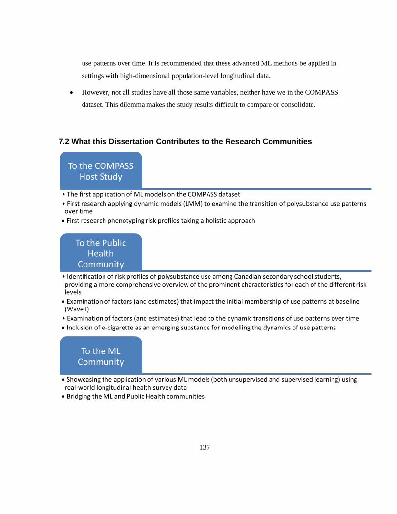
137
use patterns over time. It is recommended that these advanced ML methods be applied in
settings with high-dimensional population-level longitudinal data.
• However, not all studies have all those same variables, neither have we in the COMPASS
dataset. This dilemma makes the study results difficult to compare or consolidate.
7.2 What this Dissertation Contributes to the Research Communities
To the COMPASS Host Study
• The first application of ML models on the COMPASS dataset
• First research applying dynamic models (LMM) to examine the transition of polysubstance use patterns over time
• First research phenotyping risk profiles taking a holistic approach
To the Public Health
Community• Identification of risk profiles of polysubstance use among Canadian secondary school students, providing a more comprehensive overview of the prominent characteristics for each of the different risk levels
• Examination of factors (and estimates) that impact the initial membership of use patterns at baseline (Wave I)
• Examination of factors (and estimates) that lead to the dynamic transitions of use patterns over time
• Inclusion of e-cigarette as an emerging substance for modelling the dynamics of use patterns
To the ML Community
• Showcasing the application of various ML models (both unsupervised and supervised learning) using real-world longitudinal health survey data
• Bridging the ML and Public Health communities

138
7.3 What We Still Need to Know and How We Can Get there
• How well do our models perform?
o Internal validation: e.g., cross-replication, comparing statistical model-based methods
(e.g., LCA) vs. clustering algorithms, LTA vs. LMM
o External validation: using external data, e.g., newer waves
• What are the characteristic differences in the dynamic transition of use patterns among youth?
This will be achieved by conducting a stratified analysis with the LMM framework, e.g., sex,
race, age, urbanity, etc.
• How do the school programs and policies impact youth behaviours on polysubstance use?
This will be performed by adding the SPP data into a multilevel LMM framework upon the
availability of the software package.
• What are the risk profiles at the school level reflecting youth polysubstance use? This will be
examined using aggregated student-level data and hierarchical BE and other environmental
data available in the COMPASS study.
• Given the impact of COVID-19 on school closures and lockdown throughout the school year
of 2020-2021, it would be worthwhile to examine any rare patterns or emerging trends of
polysubstance use among Canadian secondary school students. Comparing the use patterns
and the dynamic transitions between this school year and other years would be meaningful to
public health practitioners.
7.4 Final Thoughts
This thesis epitomizes the emergence of a new and exciting field at the intersection of two research
communities, ML and Public Health. As this is also the first study of its kind to ascertain risk profiles
and dynamics of use patterns in youth polysubstance use, by employing ML approaches to the
COMPASS dataset, this research provides insights into the opportunities and possibilities ahead for
ML in Public Health. By using complex and high-dimensional longitudinal health survey data, this
thesis demonstrates the application of LMMs to evaluate the transition of youth substance use

139
patterns over time. Furthermore, this thesis describes the application of cluster analysis, one type of
unsupervised ML approach in determining the risk profiles of polysubstance use in this cohort.
Findings from studies like this can be beneficial to practitioners in the field, such as school program
managers or policymakers, in their capacity to develop interventions to prevent or remedy
polysubstance use among youth.
This thesis exemplifies one specific application of ML in public health, namely, identifying
behavioural patterns affecting health. By tackling prevalent population health issues, such as youth
substance uses investigated herein, this research contributes to advancing public health research and
practices. One of humanity’s collective responsibilities is to ensure the welfare of our youth, as they
are the future generation. Unfortunately, the current trend in polysubstance use among adolescents is
becoming a growing challenge facing many countries with severe consequences both for the
individual and our society. Thus, an aspiration behind this thesis is to provide a means to accelerate
the research that can provide insights to design and implement programs and interventions for those
directly affected by the detrimental effects of youth polysubstance use.

140
Bibliography
1. John Freeman, Matthew King, William Picket. Health Behaviour in School-aged Children
(HBSC) in Canada. 2016.
2. Health Canada. Summary of results for the Canadian Student Tobacco, Alcohol and Drugs
Survey 2018-19. 2019 Dec.
3. Connor JP, Gullo MJ, White A, Kelly AB. Polysubstance use: diagnostic challenges, patterns
of use and health. Current opinion in psychiatry. 2014;27(4):269–75.
4. Lopez-Quintero C, Granja K, Hawes S, Duperrouzel JC, Pacheco-Colón I, Gonzalez R.
Transition to drug co-use among adolescent cannabis users: The role of decision-making and
mental health. Addictive behaviors. 2018;85:43–50.
5. Maslowsky J, Schulenberg JE, O’Malley PM, Kloska DD. Depressive symptoms, conduct
problems, and risk for polysubstance use among adolescents: Results from US national
surveys. Mental Health and Substance Use. 2014;7(2):157–69.
6. Bohnert KM, Walton MA, Resko S, Barry KT, Chermack ST, Zucker RA, et al. Latent class
analysis of substance use among adolescents presenting to urban primary care clinics. The
American journal of drug and alcohol abuse. 2014;40(1):44–50.
7. CDC. Youth Risk Behavior Survey Data Summary & Trends Report: 2009-2019. 2019.
8. Dornbusch SM, Lin I-C, Munroe PT, Bianchi AJ. Adolescent polydrug use and violence in the
United States. International journal of adolescent medicine and health. 1999;11(3–4):197–220.
9. Wanner B, Vitaro F, Carbonneau R, Tremblay RE. Cross-lagged links among gambling,
substance use, and delinquency from midadolescence to young adulthood: additive and
moderating effects of common risk factors. Psychology of addictive behaviors. 2009;23(1):91.
10. Gervais A, O’Loughlin J, Meshefedjian G, Bancej C, Tremblay M. Milestones in the natural
course of onset of cigarette use among adolescents. Cmaj. 2006;175(3):255–61.
11. Hall W, Degenhardt L. Adverse health effects of non-medical cannabis use. The Lancet.
2009;374(9698):1383–91.
12. Armentano P. Cannabis and psychomotor performance: a rational review of the evidence and
implications for public policy. Drug testing and analysis. 2013;5(1):52–6.
13. Zuckermann AME, Williams G, Battista K, de Groh M, Jiang Y, Leatherdale ST. Trends of
poly-substance use among Canadian youth. Addictive behaviors reports. 2019;10:100189.

141
14. Zuckermann AME, Williams GC, Battista K, Jiang Y, de Groh M, Leatherdale ST. Prevalence
and correlates of youth poly-substance use in the COMPASS study. Addictive behaviors.
2020;107:106400.
15. Johnston LD, Miech RA, O’Malley PM, Bachman JG, Schulenberg JE, Patrick ME.
Monitoring the Future National Survey Results on Drug Use, 1975-2018: Overview, Key
Findings on Adolescent Drug Use. Institute for Social Research. 2019;
16. Benke K, Benke G. Artificial intelligence and big data in public health. International journal
of environmental research and public health. 2018;15(12):2796.
17. Rosella L, Fisher S, Song M. Artificial Intelligence and Machine Learning for Public Health.
2020 Oct.
18. Flaxman AD, Vos T. Machine learning in population health: Opportunities and threats. PLoS
medicine. 2018;15(11).
19. Mooney SJ, Pejaver V. Big data in public health: terminology, machine learning, and privacy.
Annual review of public health. 2018;39:95–112.
20. dos Santos BS, Steiner MTA, Fenerich AT, Lima RHP. Data Mining and Machine Learning
techniques applied to Public Health Problems: A bibliometric analysis from 2009 to 2018.
Computers & Industrial Engineering. 2019;106120.
21. Dolley S. Big data’s role in precision public health. Frontiers in public health. 2018;6:68.
22. Everitt BS, Landau S, Leese M, Stahl D. Cluster analysis 5th ed. John Wiley; 2011.
23. Embrechts MJ, Gatti CJ, Linton J, Roysam B. Hierarchical clustering for large data sets. In:
Advances in Intelligent Signal Processing and Data Mining. Springer; 2013. p. 197–233.
24. Collins LM, Sayer AG. New methods for the analysis of change. American Psychological
Association; 2001.
25. Singer JD, Willett JB, Willett JB, others. Applied longitudinal data analysis: Modeling change
and event occurrence. Oxford university press; 2003.
26. Killewo J, Heggenhougen K, Quah SR. Epidemiology and demography in public health.
Academic Press; 2010.
27. Bartolucci F, Farcomeni A, Pennoni F. Latent Markov models for longitudinal data. CRC
Press; 2012.
28. Diggle P, Diggle PJ, Heagerty P, Liang K-Y, Heagerty PJ, Zeger S, et al. Analysis of
longitudinal data. Oxford University Press; 2002.
142
29. Fitzmaurice G, Molenberghs G. Advances in longitudinal data analysis: an historical
perspective. Longitudinal data analysis. 2009;3–30.
30. Johnstone IM, Titterington DM. Statistical challenges of high-dimensional data. The Royal
Society Publishing; 2009.
31. Government of Canada. The Health Behaviour in School-aged Children (HBSC) study in
Canada. 2021.
32. Tomczyk S, Isensee B, Hanewinkel R. Latent classes of polysubstance use among
adolescents—a systematic review. Drug and Alcohol Dependence. 2016;160:12–29.
33. Merrin GJ, Leadbeater B. Do classes of polysubstance use in adolescence differentiate growth
in substances used in the transition to young adulthood? Substance use & misuse.
2018;53(13):2112–24.
34. Health Canada. Canadian Tobacco, Alcohol and Drugs Survey (CTADS): summary of results
for 2017. 2019 Jan.
35. Hopfer S, Tan X, Wylie JL. A social network–informed latent class analysis of patterns of
substance use, sexual behavior, and mental health: Social Network Study III, Winnipeg,
Manitoba, Canada. American journal of public health. 2014;104(5):834–9.
36. Fallu J-S, N-Brière F, Janosz M. Latent classes of substance use in adolescent cannabis users:
predictors and subsequent substance-related harm. Frontiers in psychiatry. 2014;5:9.
37. Moss HB, Chen CM, Yi H. Early adolescent patterns of alcohol, cigarettes, and marijuana
polysubstance use and young adult substance use outcomes in a nationally representative
sample. Drug and alcohol dependence. 2014;136:51–62.
38. Peters EN, Budney AJ, Carroll KM. Clinical correlates of co-occurring cannabis and tobacco
use: A systematic review. Addiction. 2012;107(8):1404–17.
39. Kelly AB, Evans-Whipp TJ, Smith R, Chan GCK, Toumbourou JW, Patton GC, et al. A
longitudinal study of the association of adolescent polydrug use, alcohol use and high school
non-completion. Addiction. 2015;110(4):627–35.
40. Strunin L, D\’\iaz-Mart\’\inez A, D\’\iaz-Mart\’\inez LR, Heeren T, Chen C, Winter M, et al.
Age of onset, current use of alcohol, tobacco or marijuana and current polysubstance use
among male and female Mexican students. Alcohol and Alcoholism. 2017;52(5):564–71.
143
41. Banks DE, Rowe AT, Mpofu P, Zapolski TCB. Trends in typologies of concurrent alcohol,
marijuana, and cigarette use among US adolescents: An ecological examination by sex and
race/ethnicity. Drug and alcohol dependence. 2017;179:71–7.
42. Jongenelis M, Pettigrew S, Lawrence D, Rikkers W. Factors associated with poly drug use in
adolescents. Prevention Science. 2019;20(5):695–704.
43. Valente JY, Cogo-Moreira H, Sanchez ZM. Gradient of association between parenting styles
and patterns of drug use in adolescence: A latent class analysis. Drug and alcohol dependence.
2017;180:272–8.
44. Silveira ML, Green VR, Iannaccone R, Kimmel HL, Conway KP. Patterns and correlates of
polysubstance use among US youth aged 15–17 years: wave 1 of the Population Assessment
of Tobacco and Health (PATH) Study. Addiction. 2019;114(5):907–16.
45. Cranford JA, McCabe SE, Boyd CJ. Adolescents’ nonmedical use and excessive medical use
of prescription medications and the identification of substance use subgroups. Addictive
behaviors. 2013;38(11):2768–71.
46. Rose RA, Evans CBR, Smokowski PR, Howard MO, Stalker KL. Polysubstance Use Among
Adolescents in a Low Income, Rural Community: Latent Classes for Middle-and High-School
Students. The Journal of Rural Health. 2018;34(3):227–35.
47. Connell CM, Gilreath TD, Hansen NB. A multiprocess latent class analysis of the co-
occurrence of substance use and sexual risk behavior among adolescents. Journal of studies on
alcohol and drugs. 2009;70(6):943–51.
48. Gilreath TD, Astor RA, Estrada JN, Johnson RM, Benbenishty R, Unger JB. Substance use
among adolescents in California: A latent class analysis. Substance use & misuse. 2014;49(1–
2):116–23.
49. Patton GC, Coffey C, Carlin JB, Degenhardt L, Lynskey M, Hall W. Cannabis use and mental
health in young people: cohort study. Bmj. 2002;325(7374):1195–8.
50. Mathers M, Toumbourou JW, Catalano RF, Williams J, Patton GC. Consequences of youth
tobacco use: a review of prospective behavioural studies. Addiction. 2006;101(7):948–58.
51. Lesjak V, Stanojević-Jerković O. Physical activity, sedentary behavior and substance use
among adolescents in slovenian urban area. Slovenian Journal of Public Health.
2015;54(3):168.

144
52. Isralowitz RE, Trostler N. Substance use: toward an understanding of its relation to nutrition-
related attitudes and behavior among Israeli high school youth. Journal of adolescent health.
1996;19(3):184–9.
53. White J, Walton D, Walker N. Exploring comorbid use of marijuana, tobacco, and alcohol
among 14 to 15-year-olds: findings from a national survey on adolescent substance use. BMC
public health. 2015;15(1):1–9.
54. Su J, Supple AJ, Kuo SI-C. The role of individual and contextual factors in differentiating
substance use profiles among adolescents. Substance use & misuse. 2018;53(5):734–43.
55. Pettigrew S, Jongenelis M, Lawrence D, Rikkers W. Common and differential factors
associated with abstinence and poly drug use among Australian adolescents. International
Journal of Drug Policy. 2017;50:41–7.
56. Tomczyk S, Hanewinkel R, Isensee B. Multiple substance use patterns in adolescents—A
multilevel latent class analysis. Drug and alcohol dependence. 2015;155:208–14.
57. White A, Chan GCK, Quek L-H, Connor JP, Saunders JB, Baker P, et al. The topography of
multiple drug use among adolescent Australians: Findings from the National Drug Strategy
Household Survey. Addictive Behaviors. 2013;38(4):2068–73.
58. Hale D, Viner R. Trends in the prevalence of multiple substance use in adolescents in
England, 1998–2009. Journal of Public Health. 2013;35(3):367–74.
59. Leatherdale ST, Brown KS, Carson V, Childs RA, Dubin JA, Elliott SJ, et al. The COMPASS
study: a longitudinal hierarchical research platform for evaluating natural experiments related
to changes in school-level programs, policies and built environment resources. BMC Public
Health. 2014;14(1):331.
60. Reel B, Bredin C, Leatherdale ST. COMPASS year 5 and 6 school recruitment and retention
compass technical report series. In: Compass technical report series. 2018.
61. About the COMPASS System [Internet]. [cited 2021 Jun 18]. Available from:
https://uwaterloo.ca/compass-system/about
62. Reel B. Battista K. Bredin C. & Leatherdale S.T. COMPASS Questionnaire Changes from
Year 1 to Year 7: Technical Report Series. 2019.
63. Aleyan S, Gohari MR, Cole AG, Leatherdale ST. Exploring the Bi-Directional Association
between Tobacco and E-Cigarette Use among Youth in Canada. International journal of
environmental research and public health. 2019;16(21):4256.

145
64. Aleyan S, Ferro MA, Hitchman SC, Leatherdale ST. Does having one or more smoking
friends mediate the transition from e-cigarette use to cigarette smoking: a longitudinal study of
Canadian youth. Cancer Causes & Control. 2021;32(1):67–74.
65. Gohari MR, Cook RJ, Dubin JA, Leatherdale ST. Identifying patterns of alcohol use among
secondary school students in Canada: a multilevel latent class analysis. Addictive behaviors.
2020;100:106120.
66. Romano I, Williams G, Butler A, Aleyan S, Patte KA, Leatherdale ST. Psychological and
Behavioural Correlates of Cannabis use among Canadian Secondary School Students:
Findings from the COMPASS Study. Canadian Journal of Addiction. 2019;10(3):10–21.
67. Halladay J, Woock R, El-Khechen H, Munn C, MacKillop J, Amlung M, et al. Patterns of
substance use among adolescents: a systematic review. Drug and alcohol dependence.
2020;108222.
68. Collins LM, Lanza ST. Latent class and latent transition analysis: With applications in the
social, behavioral, and health sciences. Vol. 718. John Wiley & Sons; 2009.
69. Mak KK, Lee K, Park C. Applications of machine learning in addiction studies: A systematic
review. Psychiatry research. 2019;275:53–60.
70. Jing Y, Hu Z, Fan P, Xue Y, Wang L, Tarter RE, et al. Analysis of substance use and its
outcomes by machine learning I. Childhood evaluation of liability to substance use disorder.
Drug and alcohol dependence. 2020;206:107605.
71. Gray HM, Tom MA, LaPlante DA, Shaffer HJ. Using opinions and knowledge to identify
natural groups of gambling employees. Journal of gambling studies. 2015;31(4):1753–66.
72. Ashok A, Guruprasad M, Prakash CO, Shylaja SS. A Machine Learning Approach for Disease
Surveillance and Visualization using Twitter Data. In: 2019 International Conference on
Computational Intelligence in Data Science (ICCIDS). 2019. p. 1–6.
73. Elliott L, Haddock CK, Campos S, Benoit E. Polysubstance use patterns and novel synthetics:
A cluster analysis from three US cities. PloS one. 2019;14(12):e0225273.
74. Sun J, Bi J, Chan G, Oslin D, Farrer L, Gelernter J, et al. Improved methods to identify stable,
highly heritable subtypes of opioid use and related behaviors. Addictive behaviors.
2012;37(10):1138–44.
75. Wang Y, Chen R, Ghosh J, Denny JC, Kho A, Chen Y, et al. Rubik: Knowledge guided tensor
factorization and completion for health data analytics. In: Proceedings of the 21th ACM
146
SIGKDD International Conference on Knowledge Discovery and Data Mining. 2015. p. 1265–
74.
76. Daniel J. Bauer, Patrick J. Curran. Conducting Longitudinal Data Analysis: Knowing What to
Do and Learning How to Do It. 2019.
77. Koenig LB, Haber JR, Jacob T. Transitions in alcohol use over time: a survival analysis. BMC
psychology. 2020;8(1):1–13.
78. Elisa Bream. Chapter 1 Introduction What are longitudinal and panel data? Benefits and
drawbacks of longitudinal data Longitudinal data models Historical notes.
https://slideplayer.com/slide/1718538/. 2014.
79. Ellie Ringrose. Panel and Time Series Cross Section Models.
https://slideplayer.com/slide/1718542/. 2014.
80. SAMHDA. National Survey on Drug Use and Health (NSDUH). 2019.
81. Bray BC, Smith RA, Piper ME, Roberts LJ, Baker TB. Transitions in smokers’ social
networks after quit attempts: A latent transition analysis. Nicotine & Tobacco Research.
2016;18(12):2243–51.
82. Hsiao C. Analysis of panel data. Cambridge university press; 2014.
83. Juang BH, Rabiner LR. Hidden Markov models for speech recognition. Technometrics.
1991;33(3):251–72.
84. Westhead DR, Vijayabaskar MS. Hidden Markov Models: Methods and Protocols. Springer;
2017.
85. Vijayabaskar MS. Introduction to hidden Markov models and its applications in biology. In:
Hidden Markov Models. Springer; 2017. p. 1–12.
86. Wiggins LM. Panel analysis: Latent probability models for attitude and behavior processes.
1973;
87. Bartolucci F, Pennoni F, Francis B. A latent Markov model for detecting patterns of criminal
activity. Journal of the royal statistical society: series A (statistics in society).
2007;170(1):115–32.
88. Bartolucci F. Likelihood inference for a class of latent Markov models under linear hypotheses
on the transition probabilities. Journal of the Royal Statistical Society: Series B (Statistical
Methodology). 2006;68(2):155–78.

147
89. Bartolucci F, Lupparelli M, Montanari GE, others. Latent Markov model for longitudinal
binary data: An application to the performance evaluation of nursing homes. The Annals of
Applied Statistics. 2009;3(2):611–36.
90. Wouterse B, Huisman M, Meijboom BR, Deeg DJH, Polder JJ. Modeling the relationship
between health and health care expenditures using a latent Markov model. Journal of Health
Economics. 2013;32(2):423–39.
91. Gil J, Li Donni P, Zucchelli E. Uncontrolled diabetes and health care utilisation: A bivariate
latent Markov model approach. Health economics. 2019;28(11):1262–76.
92. Mitchell CM, Beals J, Whitesell NR, of Indian Teens Pathways of choice teams V. Alcohol
use among American Indian high school youths from adolescence and young adulthood: A
latent Markov model. Journal of studies on alcohol and drugs. 2008;69(5):666–75.
93. Rijmen F, Vansteelandt K, de Boeck P. Latent class models for diary method data: Parameter
estimation by local computations. Psychometrika. 2008;73(2):167.
94. Bartolucci F, Solis-Trapala IL. Multidimensional latent Markov models in a developmental
study of inhibitory control and attentional flexibility in early childhood. Psychometrika.
2010;75(4):725–43.
95. Bartolucci F, Farcomeni A. A multivariate extension of the dynamic logit model for
longitudinal data based on a latent Markov heterogeneity structure. Journal of the American
Statistical Association. 2009;104(486):816–31.
96. Hox JJ. Multilevel regression and multilevel structural equation modeling. The Oxford
handbook of quantitative methods. 2013;2(1):281–94.
97. Lesa Hoffman. Measuring Individual Change: A Gentle Introduction to the Pros and Cons of
Modern Models. 2014 Dec.
98. Kaplan D. Structural equation modeling: Foundations and extensions. Vol. 10. Sage
Publications; 2008.
99. Montanari GE, Doretti M, Bartolucci F. Statistical assessment of public health care services: A
multilevel latent Markov model. In: Proceedings of the 8th scientific conference on innovation
and society, statistical methods for evaluation and quality. 2017.
100. Bartolucci F, Pennoni F, Vittadini G. Assessment of school performance through a multilevel
latent Markov Rasch model. Journal of Educational and Behavioral Statistics.
2011;36(4):491–522.
148
101. Williford A, Zinn A. Classroom-level differences in child-level bullying experiences:
Implications for prevention and intervention in school settings. Journal of the Society for
Social Work and Research. 2018;9(1):23–48.
102. Koukounari A, Moustaki I, Grassly NC, Blake IM, Basáñez M-G, Gambhir M, et al. Using a
nonparametric multilevel latent Markov model to evaluate diagnostics for trachoma. American
journal of epidemiology. 2013;177(9):913–22.
103. Khoury MJ, Iademarco MF, Riley WT. Precision public health for the era of precision
medicine. American journal of preventive medicine. 2016;50(3):398.
104. Morgenstern JD, Buajitti E, O’Neill M, Piggott T, Goel V, Fridman D, et al. Predicting
population health with machine learning: a scoping review. BMJ open. 2020;10(10):e037860.
105. Morgenstern JD, Rosella LC, Daley MJ, Goel V, Schünemann HJ, Piggott T. “AI’s gonna
have an impact on everything in society, so it has to have an impact on public health”: a
fundamental qualitative descriptive study of the implications of artificial intelligence for
public health. BMC Public Health. 2021;21(1):1–14.
106. Lee D, Yoon SN. Application of Artificial Intelligence-Based Technologies in the Healthcare
Industry: Opportunities and Challenges. International Journal of Environmental Research and
Public Health. 2021;18(1):271.
107. Lau EY, Faulkner G, Qian W, Leatherdale ST. Longitudinal associations of parental and peer
influences with physical activity during adolescence: findings from the COMPASS study.
Health promotion and chronic disease prevention in Canada: research, policy and practice.
2016;36(11):235.
108. Publications [Internet]. 2021 [cited 2021 Jun 18]. Available from:
https://uwaterloo.ca/compass-system/publications
109. Lee Y, Kim Y, Leatherdale ST, Chung H. Multilevel latent class profile analysis: An
application to stage-sequential patterns of alcohol use in a sample of Canadian youth.
Evaluation & the Health Professions. 2021;44(1):50–60.
110. Hammami N, Chaurasia A, Bigelow P, Leatherdale ST. A gender-stratified, multilevel latent
class assessment of chronic disease risk behaviours’ association with Body Mass Index among
youth in the COMPASS study. Preventive medicine. 2019;126:105758.

149
111. Laxer RE, Brownson RC, Dubin JA, Cooke M, Chaurasia A, Leatherdale ST. Clustering of
risk-related modifiable behaviours and their association with overweight and obesity among a
large sample of youth in the COMPASS study. BMC public health. 2017;17(1):1–11.
112. Holzinger A. Interactive machine learning for health informatics: when do we need the
human-in-the-loop? Brain Informatics. 2016;3(2):119–31.
113. Thompson-Haile A, Leatherdale ST. Student-level data collection procedures. In: Compass
technical report series. 2013.
114. Bredin C, Leatherdale ST. Methods for linking COMPASS student-level data over time.
Waterloo, Ontario: University of Waterloo. 2013;
115. Kearney KA, Hopkins RH, Mauss AL, Weisheit RA. Self-generated identification codes for
anonymous collection of longitudinal questionnaire data. Public Opinion Quarterly.
1984;48(1B):370–8.
116. McCarthy WJ, Mistry R, Lu Y, Patel M, Zheng H, Dietsch B. Density of tobacco retailers near
schools: effects on tobacco use among students. American journal of public health.
2009;99(11):2006–13.
117. Cole AG, Aleyan S, Leatherdale ST. Exploring the association between e-cigarette retailer
proximity and density to schools and youth e-cigarette use. Preventive medicine reports.
2019;15:100912.
118. Shortt NK, Tisch C, Pearce J, Richardson EA, Mitchell R. The density of tobacco retailers in
home and school environments and relationship with adolescent smoking behaviours in
Scotland. Tobacco control. 2016;25(1):75–82.
119. Dr. Deng. Single Imputation Methods for Missing Data: LOCF, BOCF, LRCF (Last Rank
Carried Forward), and NOCB (Next Observation Carried Backward). 2021.
120. Maaten L van der, Hinton G. Visualizing data using t-SNE. Journal of machine learning
research. 2008;9(Nov):2579–605.
121. Nikolay Oskolkov. How to tune hyperparameters of tSNE. 2019.
122. Shi W, Zeng W. Genetic k-means clustering approach for mapping human vulnerability to
chemical hazards in the industrialized city: a case study of Shanghai, China. International
journal of environmental research and public health. 2013;10(6):2578–95.
123. Dudoit S, Fridlyand J. A prediction-based resampling method for estimating the number of
clusters in a dataset. Genome biology. 2002;3(7):research0036–1.

150
124. Thalamuthu A, Mukhopadhyay I, Zheng X, Tseng GC. Evaluation and comparison of gene
clustering methods in microarray analysis. Bioinformatics. 2006;22(19):2405–12.
125. Rousseeuw PJ. Silhouettes: a graphical aid to the interpretation and validation of cluster
analysis. Journal of computational and applied mathematics. 1987;20:53–65.
126. Archer KJ. glmpathcr: An R Package for Ordinal Response Prediction in High-dimensional
Data Settings. 2015;
127. Bartolucci F, Farcomeni A, Pennoni F. Latent Markov models: a review of a general
framework for the analysis of longitudinal data with covariates. Test. 2014;23(3):433–65.
128. Pongsapukdee V, Sukgumphaphan S. Goodness of fit of cumulative logit models for ordinal
response categories and nominal explanatory variables with two-factor interaction. Science,
Engineering and Health Studies (Former name: Silpakorn University Science and Technology
Journal). 2007;29–38.
129. Kaufman L, Rousseeuw PJ. Fuzzy analysis (program FANNY). Finding Groups in Data: An
Introduction to Cluster Analysis NJ: John Wiley & Sons. 2005;164–98.
130. West AB, Bittel KM, Russell MA, Evans MB, Mama SK, Conroy DE. A systematic review of
physical activity, sedentary behavior, and substance use in adolescents and emerging adults.
Translational behavioral medicine. 2020;10(5):1155–67.
131. Radloff LS. The CES-D scale: A self-report depression scale for research in the general
population. Applied psychological measurement. 1977;1(3):385–401.
132. Cairns KE, Yap MBH, Pilkington PD, Jorm AF. Risk and protective factors for depression
that adolescents can modify: a systematic review and meta-analysis of longitudinal studies.
Journal of affective disorders. 2014;169:61–75.
133. Morean ME, Kong G, Camenga DR, Cavallo DA, Simon P, Krishnan-Sarin S. Latent class
analysis of current e-cigarette and other substance use in high school students. Drug and
alcohol dependence. 2016;161:292–7.
134. Choi HJ, Lu Y, Schulte M, Temple JR. Adolescent substance use: Latent class and transition
analysis. Addictive behaviors. 2018;77:160–5.
135. Lanza ST, Patrick ME, Maggs JL. Latent transition analysis: Benefits of a latent variable
approach to modeling transitions in substance use. Journal of drug issues. 2010;40(1):93–120.
136. Merrin GJ, Thompson K, Leadbeater BJ. Transitions in the use of multiple substances from
adolescence to young adulthood. Drug and alcohol dependence. 2018;189:147–53.

151
137. Danks D, London AJ. Algorithmic Bias in Autonomous Systems. In: IJCAI. 2017. p. 4691–7.
138. Zhang BH, Lemoine B, Mitchell M. Mitigating unwanted biases with adversarial learning. In:
Proceedings of the 2018 AAAI/ACM Conference on AI, Ethics, and Society. 2018. p. 335–40.
139. Rob Thomas. The AI Ladder. 2019.
140. Ashish N, Sriram S. Accelerating AI Modernization with Data Infrastructure. 2021 Feb.
141. Simran Kaur Arora. 10 Best Machine Learning Certification for 2021. 2021 Jul 9;
142. Elton-Marshall T, Leatherdale ST, Manske SR, Wong K, others. Research methods of the
youth smoking survey (YSS). Chronic diseases and injuries in Canada. 2011;32(1).
143. Battista K, Qian W, Bredin C, Leatherdale ST, others. Student data linkage over multiple
years. COMPASS Tech Rep Ser. 2019;6:1–10.
144. David Talby. Lessons learned turning machine learning models into real products and
services. 2018.
145. Bastiane Huang. How to Manage Machine Learning Products. 2019.
146. Cui P, Shen Z, Li S, Yao L, Li Y, Chu Z, et al. Causal Inference Meets Machine Learning. In:
Proceedings of the 26th ACM SIGKDD International Conference on Knowledge Discovery &
Data Mining. 2020. p. 3527–8.
147. Pearl J. The seven tools of causal inference, with reflections on machine learning.
Communications of the ACM. 2019;62(3):54–60.
148. Prosperi M, Guo Y, Sperrin M, Koopman JS, Min JS, He X, et al. Causal inference and
counterfactual prediction in machine learning for actionable healthcare. Nature Machine
Intelligence. 2020;2(7):369–75.
149. Schölkopf B, Locatello F, Bauer S, Ke NR, Kalchbrenner N, Goyal A, et al. Toward causal
representation learning. Proceedings of the IEEE. 2021;109(5):612–34.
150. Wayne W. LaMorte & Lisa Sullivan. Confounding and Effect Measure Modification.
151. Kettenring JR. A patent analysis of cluster analysis. Applied Stochastic Models in Business
and Industry. 2009;25(4):460–7.
152. Nasibov EN, Ulutagay G. Comparative clustering analysis of bispectral index series of brain
activity. Expert Systems with Applications. 2010;37(3):2495–504.
153. Gower JC, Legendre P. Metric and Euclidean properties of dissimilarity coefficients. Journal
of classification. 1986;3(1):5–48.
154. SB. Boruta. 2016.
152
155. Wattenberg M, ViÈgas F, Johnson I. How to use t-SNE effectively. Distillhttp. distill
pub/2016/misread-tsne. 2016;
156. Ketchen DJ, Shook CL. The application of cluster analysis in strategic management research:
an analysis and critique. Strategic management journal. 1996;17(6):441–58.
157. Larson RC, Sadiq G. Facility locations with the Manhattan metric in the presence of barriers
to travel. Operations Research. 1983;31(4):652–69.
158. Gower JC, Legendre P. Metric and Euclidean properties of dissimilarity coefficients. Journal
of classification. 1986;3(1):5–48.
159. Greenacre M, Hastie T. The geometric interpretation of correspondence analysis. Journal of
the American statistical association. 1987;82(398):437–47.
160. Leisch F. Neighborhood graphs, stripes and shadow plots for cluster visualization. Statistics
and Computing. 2010;20(4):457–69.
161. Tibshirani R. Regression shrinkage and selection via the lasso. Journal of the Royal Statistical
Society: Series B (Methodological). 1996;58(1):267–88.
162. F. Bartolucci. e-Rum2020 Keynote 3 - F. Bartolucci: “Latent Markov models for longit. data
in R by LMest package.” 2020.
163. Zucchini W, MacDonald IL, Langrock R. Hidden Markov models for time series: an
introduction using R. CRC press; 2017.
164. Baum LE, Petrie T, Soules G, Weiss N. A maximization technique occurring in the statistical
analysis of probabilistic functions of Markov chains. The annals of mathematical statistics.
1970;41(1):164–71.
165. Dempster AP, Laird NM, Rubin DB. Maximum likelihood from incomplete data via the EM
algorithm. Journal of the Royal Statistical Society: Series B (Methodological). 1977;39(1):1–
22.
166. Bozdogan H. Model selection and Akaike’s information criterion (AIC): The general theory
and its analytical extensions. Psychometrika. 1987;52(3):345–70.
167. Colombi R, Forcina A. Marginal regression models for the analysis of positive association of
ordinal response variables. Biometrika. 2001;88(4):1007–19.
168. Viterbi A. Error bounds for convolutional codes and an asymptotically optimum decoding
algorithm. IEEE transactions on Information Theory. 1967;13(2):260–9.

153
169. Altman RM. Mixed hidden Markov models: an extension of the hidden Markov model to the
longitudinal data setting. Journal of the American Statistical Association. 2007;102(477):201–
10.

154
Appendix A
The COMPASS Questionnaire (2017-18)

155
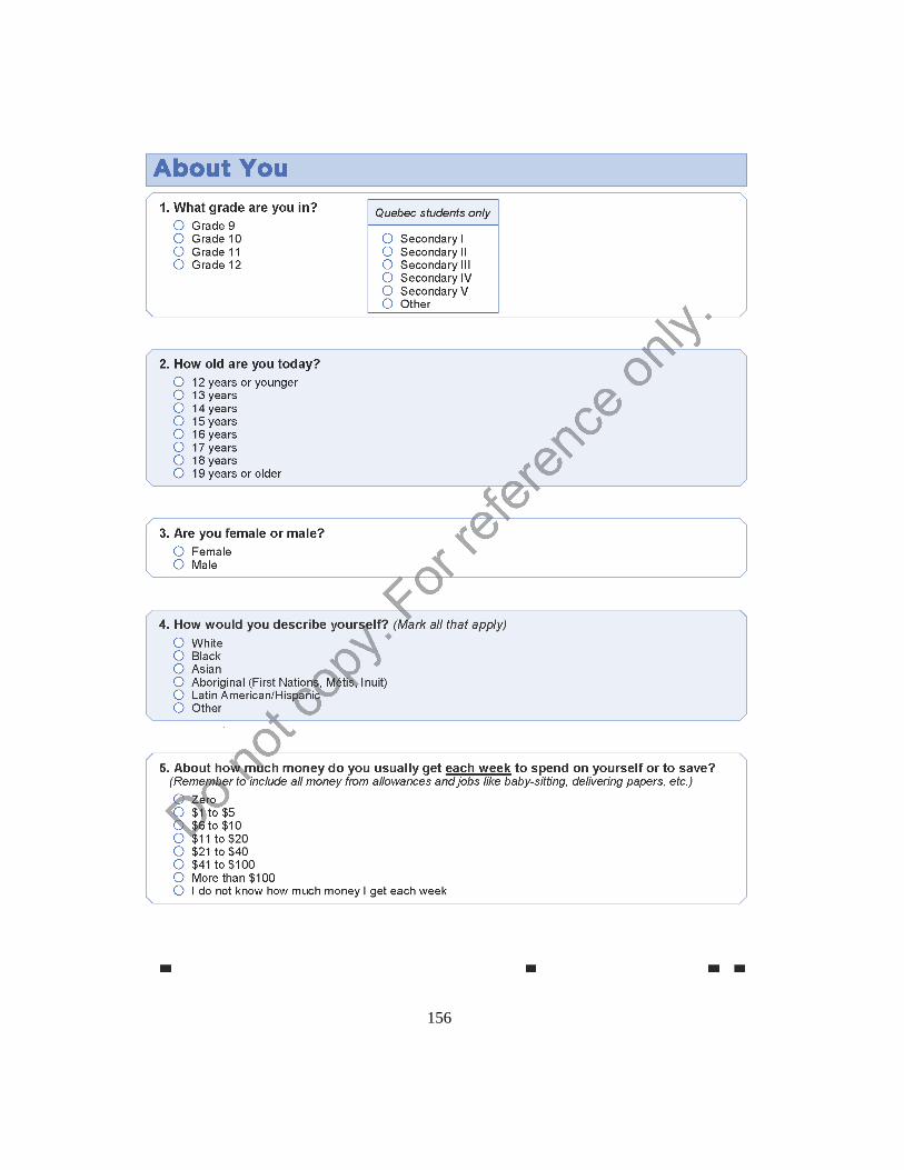
156

157
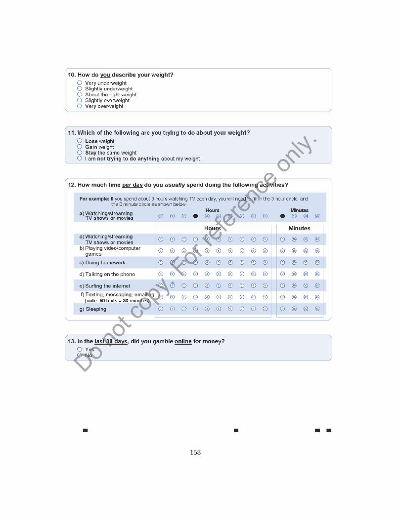
158
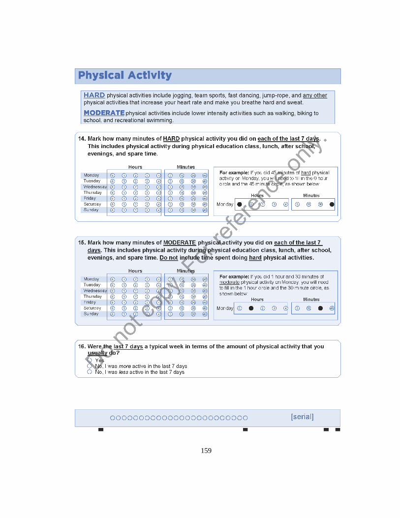
159

160

161

162
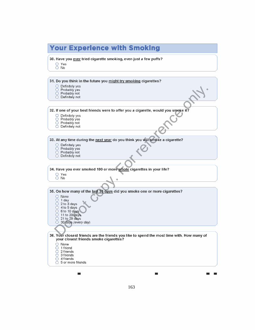
163

164
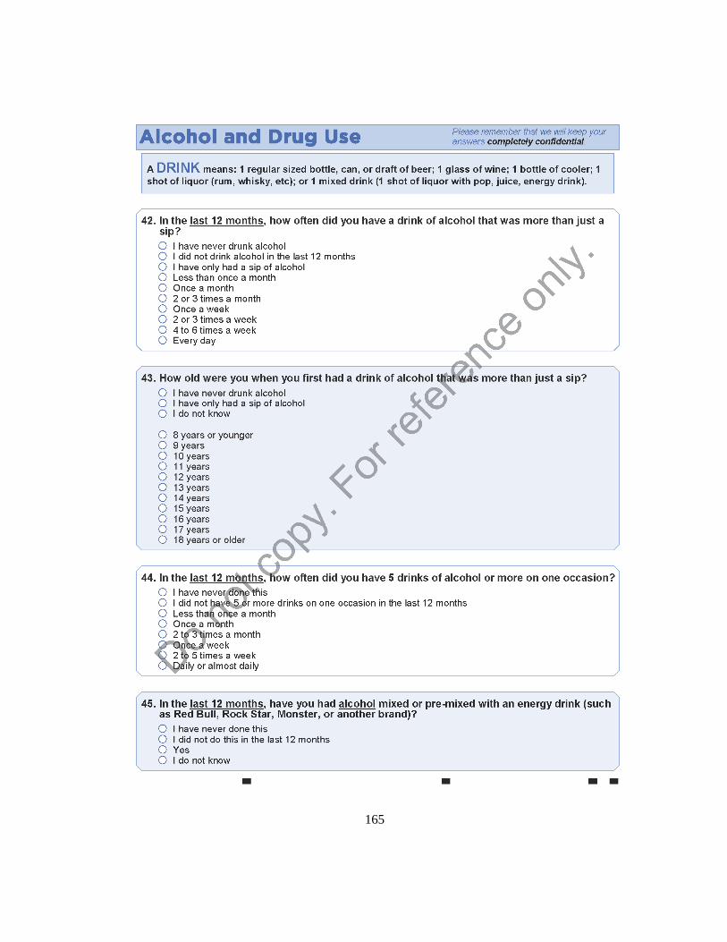
165

166

167

168
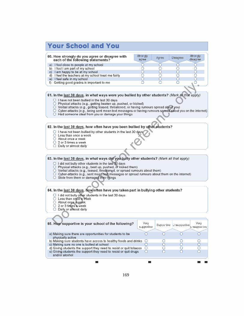
169
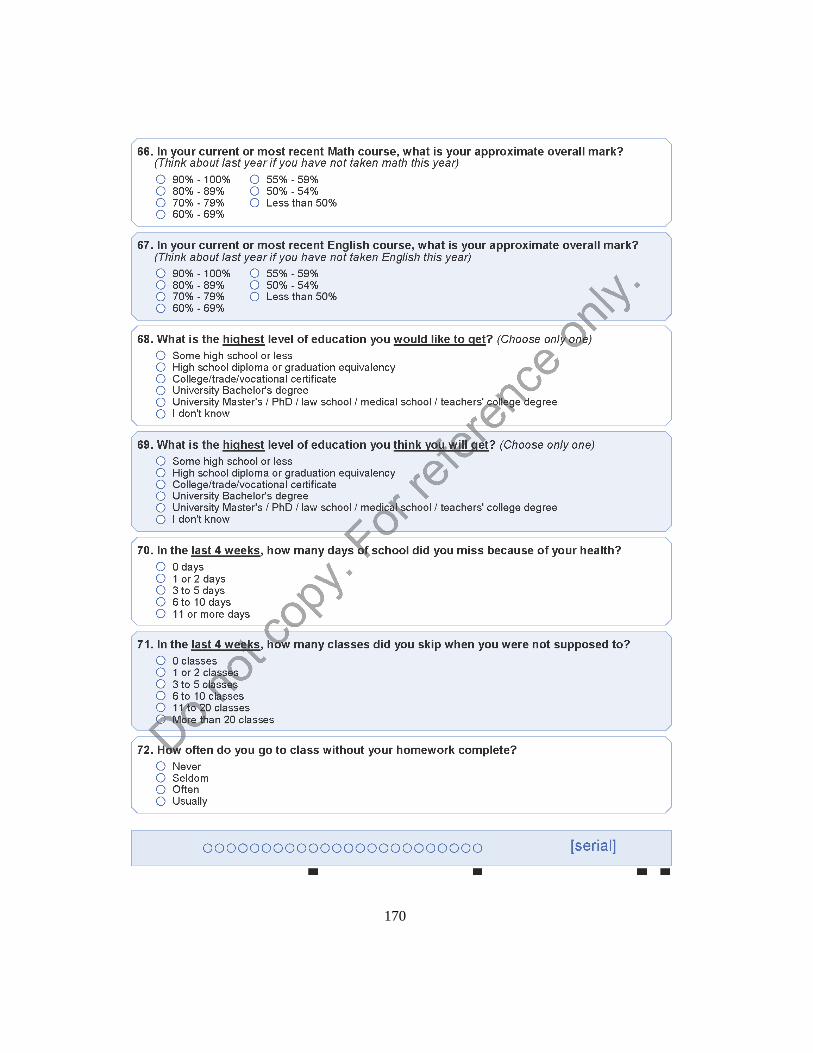
170

171
Appendix B
Agglomerative Clustering Linkage Methods (Dissimilarity
Measures)
Single Linkage (Nearest Neighbor)
Minimum distance or dissimilarity between nearest data points in clusters
𝐷(𝑘1, 𝑘2) = min 𝐷(𝑥1, 𝑥2) (3)
Complete Linkage (Furthest Neighbor)
Maximum distance or dissimilarity between furthest data points in clusters
𝐷(𝑘1, 𝑘2) = max 𝐷(𝑥1, 𝑥2) (4)
Average Linkage (UPGMA)
The average distance of all pairs of data points between clusters
𝐷(𝑘1, 𝑘2) =1
|𝑘1|
1
|𝑘2|∑ 𝐷(𝑥1, 𝑥2) (5)

172
Centroid Method (UPGMC)
Squared Euclidean distance between centroids of clusters, combining clusters with minimum
distance between centroids of the two clusters
Ward’s Method (Minimum Sum of Squares)
It aims to minimize the total within-cluster variance, combining clusters where an increase in
within-cluster variance to the minimal degree.
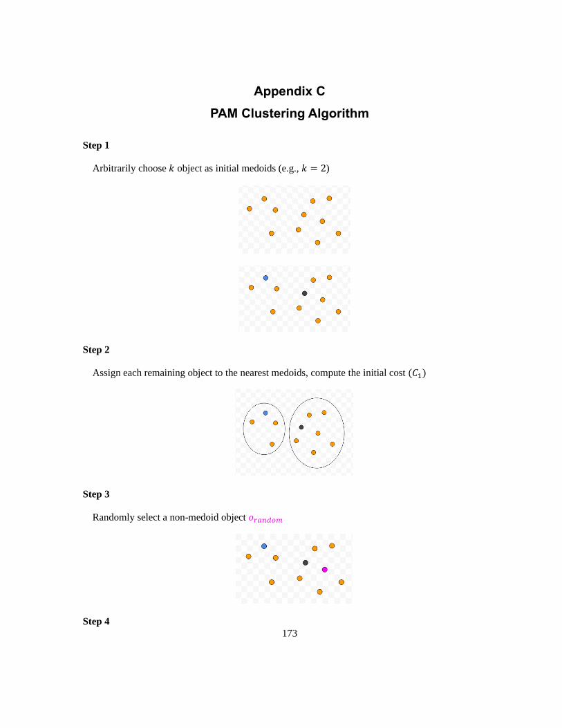
173
Appendix C
PAM Clustering Algorithm
Step 1
Arbitrarily choose 𝑘 object as initial medoids (e.g., 𝑘 = 2)
Step 2
Assign each remaining object to the nearest medoids, compute the initial cost (𝐶1)
Step 3
Randomly select a non-medoid object 𝑜𝑟𝑎𝑛𝑑𝑜𝑚
Step 4

174
Swap medoid 𝑚 and non-medoid object 𝑜𝑟𝑎𝑛𝑑𝑜𝑚, compute the total cost of swapping (𝐶2),
evaluate if cost function decreases (𝐶2 < 𝐶1)
Step 5
Repeat Steps 2-4 until the total cost of swapping is not improving anymore

175
Appendix D
Fuzzy Clustering Algorithms
Fuzzy C-Means (FCM)
The FCM algorithm applies a weighted sum-of-squares criterion for continuous data. The FCM
clustering algorithm calculates the optimal membership degree by minimizing the Euclidean distance
between the data element and the cluster centre (22), expressed as
∑ ∑ u(i, v)t 𝑑2(x𝑖, 𝑚𝑣)
𝑛
𝑖=1
𝑘
𝑣=1
(6)
where 𝑛 is the sample size, 𝑘 is the number of clusters, 𝑡 is the fuzzifier, u(i, v)t is the membership,
and 𝑑2(x𝑖, 𝑚𝑣) is the Euclidean distance between subject 𝑖 and the cluster center 𝑚𝑣. The fuzzifier 𝑡
affects the distribution of the final membership; 𝑡 = 1 leads to the hard clustering (i.e., crisp
solution), and a default setting of 𝑡 = 2 for soft clustering (fuzzy clustering). The applications of the
FCM algorithm in the health domain have been published in the literature. For instance, Kettenring
(2009) implemented it in the immediate valuation of patient portfolio assets with cluster analysis
(150). A fuzzy version of density-based spatial clustering was applied by Nasibov and Ulutagay
(2010) for comparison with fuzzy k-means (151).
Like any fuzzy clustering, data elements can belong to any cluster with a certain degree of
membership. It provides a more detailed description of the objects in the cluster. In addition, the time
complexity is low. The FCM algorithm also has some disadvantages: 1) it is sensitive to outliers and
initial centroid; 2) different initialization may lead to different clustering results; 3) the FCM
algorithm can become trapped into local maxima resulting in the final clustering being in a local
optimum instead of global maxima.
FANNY (Fuzzy ANalYsis)
Another well-known fuzzy algorithm, FANNY, minimizes the objective function
∑ ∑u(i, v)r u(j, v)r d(i, j))
(2 ∑ u(j, v)r𝑗 )
𝑛
𝑖,𝑗=1
𝑘
𝑣=1
(7)
where 𝑛 is the sample size, 𝑘 is the number of clusters, 𝑟 is the membership exponent, and 𝑑(𝑖, 𝑗) is
the dissimilarity between subjects 𝑖 and 𝑗. Increasingly crisper clustering can be achieved when 𝑟 is
176
close to 1 and complete fuzziness when 𝑟 approaches infinity (129). Further note that even the default
value, 𝑟 = 2, will lead to complete fuzziness, that is, the degree of membership 𝑢(𝑖, 𝑣) = 1
𝑘. FANNY
is more robust to non-spherical clusters than other fuzzy clustering algorithms, accepting a proximity
matrix 𝑑(𝑖, 𝑗) instead of estimating central values, i.e., Euclidean distances as in the FCM algorithm
(22).
Given the mixed type of COMPASS data, with most of the data being categorical, different
dissimilarity matrices have experimented, and the clustering results were compared. Firstly, as part of
the clustering process, grade-of-membership (GOM) analysis assigns two or more latent subgroups
for each object based on probabilities of their cluster membership. One specific distance metric, the
Gower distance, was implemented in this study. Gower distance is calculated as the average of partial
dissimilarities between data elements, depending on the evaluated variable types (152). Each feature
has a specific standardization applied, and the distance between two individuals is the average of the
particular distances of all. Each partial dissimilarity (i.e., the Gower distance) ranges between 0 and 1.
Secondly, the ordinal data were treated as continuous, so the most commonly used Euclidean distance
measure can be implemented. The Euclidean distance measure is appealing because the distance
between two objects can be interpreted as physical distance obtained from multivariate used for
clustering.

177
Appendix E
Boruta Algorithm
The Boruta algorithm is an RF-based feature selection algorithm utilizing an ensemble of decision
trees. With tree-based models, a sequence of decisions (or splits) is calculated at training time. A
stopping criterion can be specified by not splitting nodes once the decision cannot bring a specific
minimum benefit to control the overfitting of the decision trees. Reduction in Gini impurity is often
defined as a benefit within this context. Corresponding to the Gini coefficient, Gini impurity indicates
the effectiveness of the classifier for a given subset of data. Non-parametric is one property of Gini
impurity, which works with any numerical data containing a large sample size for choosing input
features. The feature ranking mechanism extends the decision tree mechanism as the impurity
decreased from each feature is averaged over all the trees. The term impurity represents either the
Gini impurity or entropy for classification and the variance for regression trees. These impurity
measures are used to select the feature that best splits the dataset.
The Boruta algorithm can be described as follows (153).
Step 1: For each feature 𝑋𝑗, randomly permute it to generate a “shadow feature” (random feature)
𝑋𝑗(𝑠)
.
Step 2: Fit a random forest classifier to the original features {𝑋1, … , 𝑋𝑝} and the shadow features
{𝑋1(𝑠)
, … , 𝑋𝑝(𝑠)
}.
Step 3: Calculate feature importance on the original features {𝐻1, … , 𝐻𝑝} and the shadow features
{𝐻1(𝑠)
, … , 𝐻𝑝(𝑠)
}.
Step 4: The feature is important for a single run if its importance is higher than the maximum
importance of all shadow features, i.e., 𝐻1 > 𝐸(𝐻).
Step 5: Eliminate all features whose importance across all runs is low enough. Keep all features
whose importance across all runs are high enough.
Step 6: Repeat Steps 1-5 with all tentative features for a pre-defined number of iterations until all
features have been identified as important or rejected.
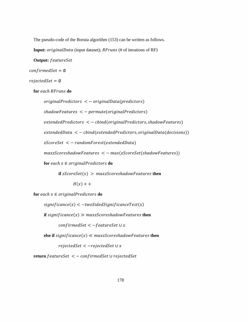
178
The pseudo-code of the Boruta algorithm (153) can be written as follows.
Input: 𝑜𝑟𝑖𝑔𝑖𝑛𝑎𝑙𝐷𝑎𝑡𝑎 (input dataset); 𝑅𝐹𝑟𝑢𝑛𝑠 (# of iterations of RF)
Output: 𝑓𝑒𝑎𝑡𝑢𝑟𝑒𝑆𝑒𝑡
𝑐𝑜𝑛𝑓𝑖𝑟𝑚𝑒𝑑𝑆𝑒𝑡 = ∅
𝑟𝑒𝑗𝑒𝑐𝑡𝑒𝑑𝑆𝑒𝑡 = ∅
for 𝑒𝑎𝑐ℎ 𝑅𝐹𝑟𝑢𝑛𝑠 do
𝑜𝑟𝑖𝑔𝑖𝑛𝑎𝑙𝑃𝑟𝑒𝑑𝑖𝑐𝑡𝑜𝑟𝑠 < − 𝑜𝑟𝑖𝑔𝑖𝑛𝑎𝑙𝐷𝑎𝑡𝑎(𝑝𝑟𝑒𝑑𝑖𝑐𝑡𝑜𝑟𝑠)
𝑠ℎ𝑎𝑑𝑜𝑤𝐹𝑒𝑎𝑡𝑢𝑟𝑒𝑠 < − 𝑝𝑒𝑟𝑚𝑢𝑡𝑒(𝑜𝑟𝑖𝑔𝑖𝑛𝑎𝑙𝑃𝑟𝑒𝑑𝑖𝑐𝑡𝑜𝑟𝑠)
𝑒𝑥𝑡𝑒𝑛𝑑𝑒𝑑𝑃𝑟𝑒𝑑𝑖𝑐𝑡𝑜𝑟𝑠 < − 𝑐𝑏𝑖𝑛𝑑(𝑜𝑟𝑖𝑔𝑖𝑛𝑎𝑙𝑃𝑟𝑒𝑑𝑖𝑐𝑡𝑜𝑟𝑠, 𝑠ℎ𝑎𝑑𝑜𝑤𝐹𝑒𝑎𝑡𝑢𝑟𝑒𝑠)
𝑒𝑥𝑡𝑒𝑛𝑑𝑒𝑑𝐷𝑎𝑡𝑎 < − 𝑐𝑏𝑖𝑛𝑑(𝑒𝑥𝑡𝑒𝑛𝑑𝑒𝑑𝑃𝑟𝑒𝑑𝑖𝑐𝑡𝑜𝑟𝑠, 𝑜𝑟𝑖𝑔𝑖𝑛𝑎𝑙𝐷𝑎𝑡𝑎(𝑑𝑒𝑐𝑖𝑠𝑖𝑜𝑛𝑠))
𝑧𝑆𝑐𝑜𝑟𝑒𝑆𝑒𝑡 < − 𝑟𝑎𝑛𝑑𝑜𝑚𝐹𝑜𝑟𝑒𝑠𝑡(𝑒𝑥𝑡𝑒𝑛𝑑𝑒𝑑𝐷𝑎𝑡𝑎)
𝑚𝑎𝑥𝑧𝑆𝑐𝑜𝑟𝑒𝑠ℎ𝑎𝑑𝑜𝑤𝐹𝑒𝑎𝑡𝑢𝑟𝑒𝑠 < − 𝑚𝑎𝑥(𝑧𝑆𝑐𝑜𝑟𝑒𝑆𝑒𝑡(𝑠ℎ𝑎𝑑𝑜𝑤𝐹𝑒𝑎𝑡𝑢𝑟𝑒𝑠))
for 𝑒𝑎𝑐ℎ 𝑥 ∈ 𝑜𝑟𝑖𝑔𝑖𝑛𝑎𝑙𝑃𝑟𝑒𝑑𝑖𝑐𝑡𝑜𝑟𝑠 do
if 𝑧𝑆𝑐𝑜𝑟𝑒𝑆𝑒𝑡(𝑥) > 𝑚𝑎𝑥𝑧𝑆𝑐𝑜𝑟𝑒𝑠ℎ𝑎𝑑𝑜𝑤𝐹𝑒𝑎𝑡𝑢𝑟𝑒𝑠 then
𝐻(𝑥) + +
for 𝑒𝑎𝑐ℎ 𝑥 ∈ 𝑜𝑟𝑖𝑔𝑖𝑛𝑎𝑙𝑃𝑟𝑒𝑑𝑖𝑐𝑡𝑜𝑟𝑠 do
𝑠𝑖𝑔𝑛𝑖𝑓𝑖𝑐𝑎𝑛𝑐𝑒(𝑥) < −𝑡𝑤𝑜𝑆𝑖𝑑𝑒𝑑𝑆𝑖𝑔𝑛𝑖𝑓𝑖𝑐𝑎𝑛𝑐𝑒𝑇𝑒𝑠𝑡(𝑥)
if 𝑠𝑖𝑔𝑛𝑖𝑓𝑖𝑐𝑎𝑛𝑐𝑒(𝑥) ≫ 𝑚𝑎𝑥𝑧𝑆𝑐𝑜𝑟𝑒𝑠ℎ𝑎𝑑𝑜𝑤𝐹𝑒𝑎𝑡𝑢𝑟𝑒𝑠 then
𝑐𝑜𝑛𝑓𝑖𝑟𝑚𝑒𝑑𝑆𝑒𝑡 < −𝑓𝑒𝑎𝑡𝑢𝑟𝑒𝑆𝑒𝑡 ∪ 𝑥
else if 𝑠𝑖𝑔𝑛𝑖𝑓𝑖𝑐𝑎𝑛𝑐𝑒(𝑥) ≪ 𝑚𝑎𝑥𝑧𝑆𝑐𝑜𝑟𝑒𝑠ℎ𝑎𝑑𝑜𝑤𝐹𝑒𝑎𝑡𝑢𝑟𝑒𝑠 then
𝑟𝑒𝑗𝑒𝑐𝑡𝑒𝑑𝑆𝑒𝑡 < −𝑟𝑒𝑗𝑒𝑐𝑡𝑒𝑑𝑆𝑒𝑡 ∪ 𝑥
return 𝑓𝑒𝑎𝑡𝑢𝑟𝑒𝑆𝑒𝑡 < − 𝑐𝑜𝑛𝑓𝑖𝑟𝑚𝑒𝑑𝑆𝑒𝑡 ∪ 𝑟𝑒𝑗𝑒𝑐𝑡𝑒𝑑𝑆𝑒𝑡

179
Appendix F
t-SNE Algorithm
A precursor method of t-SNE, Stochastic Neighbor Embedding (SNE), aims to match distributions of
distances between data elements in high- and low-dimensional space via conditional probabilities.
SNE assumes that the distances in both high- and low-dimensional space are Gaussian distributed.
SNE is performed by defining the similarities and a cost function, obtaining the gradient for the cost
function and minimizing it to get the low-dimensional map. SNE has two main drawbacks. The first
one is that it is challenging to optimize the cost function. The second one is related to the “crowding
problem,” representing the phenomenon that SNE clumps data elements nearby and moderately far
apart to make them crowded.
t-SNE with novel features represented to cost function overcome these two drawbacks. The first
improvement of t-SNE is that its cost function is symmetrized version of that in SNE, i.e.,𝑝𝑖|𝑗 = 𝑝𝑗|𝑖
and 𝑞𝑖|𝑗 = 𝑞𝑗|𝑖. The main feature in symmetric SNE is that 𝑝𝑖𝑗 = 𝑝𝑗𝑖 and 𝑝𝑖𝑖 = 𝑞𝑖𝑖 = 0 for all i,j. The
low-dimensional representation is
𝑞𝑖𝑗 =exp (−||𝑦𝑖 − 𝑦𝑗||2)
∑ exp (−||𝑦𝑘 − 𝑦𝑙||2)𝑘≠𝑙 (8)
The high-dimensional representation is
𝑝𝑖𝑗 =exp (− ||𝑥𝑖 − 𝑥𝑗||
2/2𝜎2)
∑ exp (−||𝑥𝑘 − 𝑥𝑙||2/2𝜎2)𝑘≠𝑙 (9)
The gradient of the cost function is
𝛿𝐶
𝛿𝑦𝑖= 4 ∑(𝑝𝑗𝑖 − 𝑞𝑗𝑖)(𝑦𝑖 − 𝑦𝑗)
𝑗
(10)
The second improvement in t-SNE is that t-SNE uses Student t-distribution instead of the normal
distribution to compute the similarities between data elements in a low-dimensional map. In t-SNE, a
Student t-distribution with one degree of freedom, Cauchy distribution, represents the low-
dimensional map.
𝑞𝑖𝑗 =(1 + ||𝑦𝑖 − 𝑦𝑗||2)−1
∑ (1 + ||𝑦𝑘 − 𝑦𝑙||2)−1𝑘≠𝑙
(11)

180
It is observed that this representation has no exponent and looks similar to the kernel of a t-
distribution. The main reason for using t-distribution is that it is robust to outliers. Unlike the
Gaussian distribution, it has no exponent, making it faster to evaluate. In Gaussian distribution, there
is an exponent in the kernel, making the calculation more computationally expensive. Thus, choosing
a certain t-distribution is much faster.
The gradient of the cost function via the KL divergence can be expressed as follows.
𝛿𝐶
𝛿𝑦𝑖= 4 ∑(𝑝𝑗𝑖 − 𝑞𝑗𝑖)(𝑦𝑖 − 𝑦𝑗)
𝑗
(1 + ||𝑦𝑖 − 𝑦𝑗||2)−1 (12)
The general idea of the t-SNE algorithm is that for a high-dimensional dataset ᵡ with data elements
𝑥1, 𝑥2, … 𝑥𝑛, each data element has high dimensions. The cost function parameter, perplexity, is
associated with variance σ in the cost function. The optimization parameters include the number of
iterations 𝑇, learning rate 𝜑, and momentum 𝛼(𝑡). All these components are utilized to obtain the
low-dimensional representation 𝑌.
Essentially, the t-SNE algorithm starts with pairwise affinities 𝑝𝑗|𝑖 in the high-dimensional map
with a given perplexity. Then set 𝑝𝑖𝑗 =𝑝𝑖|𝑗+𝑝𝑗|𝑖
2𝑛, where n is the number of data elements. Then sample
the initial solution for 𝑌 at the 0𝑡ℎ iteration for 𝑦1, 𝑦2, … 𝑦𝑛 from a normal distribution with the mean
0 and variance 10−4 𝑁(0, 10−4𝐼), where I represents the identity matrix. Then start with the iteration
for 𝑡 = 1 to 𝑇, which is the maximum number of iteration, first compute the lower-dimensional
affinities 𝑞𝑖𝑗, and then compute the gradient 𝛿𝐶
𝛿𝑦 through the KL divergence. Then use the gradient
descent formula to get the solution at the 𝑡𝑡ℎ solution, set
𝑦(𝑡) = 𝑦(𝑡−1) + 𝜑𝛿𝐶
𝛿𝑦+ 𝛼(𝑡)(𝑦(𝑡−1) − 𝑦(𝑡−2)) (13)
Iterate through all these processes until the maximum iteration is reached or until it converges to the
asymptotic point of the solution.
Beyond the basic t-SNE algorithm, there are modifications to reduce complexity using Barnes-Hut-
SNE approximation, a sophisticated methodology with a tree-based algorithm.
t-SNE is a popular method, which has been implemented in various software packages and
languages. The research community has widely adopted t-SNE, but there are also some criticisms

181
against it. Wattenberg, Viegas, & Johnson (2016) list some of the drawbacks of t-SNE with some
interactive visualization tools. The first drawback is that the different perplexity can lead to entirely
different clusters (154). The perplexity measure is loosely interpreted as several neighbours of a
certain point. Wattenberg, Viegas, & Johnson (2016) suggested that a perplexity between 5 and 50 is
optimal and robust within that range (154). If a perplexity is too small, then the local variations are
dominant. On the other hand, a too large perplexity leads to a dominating global change (154).
Another disadvantage of t-SNE is that cluster size does not have any meaning to it. In PCA, the X-
axis has a reasonable interpretation, and the Y-axis is the direction with the highest variance
explained. However, t-SNE does not have that intrinsic interpretation. It also tends to expand dense
clusters and contrast sparse clusters. Therefore, a dense cluster does not mean that cluster points have
minimal variance. A huge cluster does not necessarily imply those data elements have enormous
within-cluster variance.
Another criticism is that the distance between clusters might not have a clear interpretation. For
example, if two clusters are close to each other, two clusters are far apart. The inter-cluster distance
does not mean those clusters are far apart are very different from each other, or close enough clusters
are very similar.
Finally, if random noise is provided in the data, t-SNE can lead to a false positive structure in the
projection, where in reality, no structure in this random noise. Researchers need to be careful about
using t-SNE, tuning the hyperparameters, and interpreting the results. In summary, t-SNE is a
valuable tool for clustering and data visualization. It provides a better structure for high-dimensional
data. Its high flexibility leads to other drawbacks such as a lack of interpretability, not being intuitive
for parameter tuning, including perplexity, iterations, tolerance or convergence, etc.

182
Appendix G
Clustering Procedures
In a nutshell, clustering procedures include the following major steps (22).
1. Identify Objects to Cluster
Ideally, objects should be randomly sampled and representative of the cluster structure. However,
since cluster analysis is a non-inferential tool, if generalization to a larger population is not required,
it may be acceptable for over-sampling small populations.
2. Select Variables (Features)
Feature selection or extraction is one of the key steps for cluster analysis, particularly with high-
dimensional data. Feature selection refers to choosing a subset of original features from the dataset. In
contrast, feature extraction applies transformation methods to the original features to generate new
ones that are useful for analysis. Ideally, a good choice of features should distinguish various patterns
belonging to different clusters, be insensitive to outliers, and be easy to interpret. Feature extraction is
often used for dimensionality reduction and data visualization, where interpretability is not
mandatory. Considerations will also be given to data standardization and addressing multicollinearity
issues among features (155).
3. Measure Proximity
Proximity is a general term used to quantitatively measure how close (similarity) objects are to
each other or how far apart (dissimilarity or distance) they are. There exists a large number of
similarity or dissimilarity coefficients. The choice between coefficients is given by the nature of the
data, i.e., continuous or categorical.
3.1 Distance or Dissimilarity Measures
The most commonly used dissimilarity measure is Euclidean distance, which is written as
𝑑(𝑎, 𝑏) = √[∑(𝑥𝑎𝑛 − 𝑥𝑏𝑛)2
𝑘
𝑛=1
] (14)
183
where 𝑥𝑎𝑛 and 𝑥𝑏𝑛 represent for object 𝑎 and 𝑏, respectively, the value of 𝑛𝑡ℎ variable of the 𝑝-
dimensional observations. 𝑑(𝑎, 𝑏) represents physical distances between two 𝑝-dimensional
observations 𝑥𝑎 = (𝑥𝑎1, … , 𝑥𝑎𝑝) and 𝑥𝑏 = (𝑥𝑏1, … , 𝑥𝑏𝑝) in Euclidean space (22). A variety of
dissimilarity measures has been developed to accommodate different weighting of multivariate. For
example, the well-known Manhattan distance (156) is the city block distance that measures distances
on a rectilinear configuration, similar to travelling in street configuration. The correlation coefficients,
e.g., Pearson correlation, can be transformed into dissimilarities within the interval [0,1].
3.2 Similarity Measures
Similarity measures are often used for categorical data, in which the measurements are scaled
within the interval [0,1]. A similarity coefficient 𝑠(𝑎, 𝑏) describes how close the two objects 𝑎 and 𝑏
to each other. The value of 𝑠(𝑎, 𝑏) equals one represents the two objects 𝑎 and 𝑏 differ minimally for
all variables. A dissimilarity coefficient 𝑑(𝑎, 𝑏) takes a simple manner to convert its similarity
coefficient 𝑠(𝑎, 𝑏) by taking 1 − 𝑠(𝑎, 𝑏). The commonly used similarity measures for binary
variables include the matching coefficient, Jaccard coefficient, and Gower and Legendre (157).
4. Choose Clustering Algorithm
Appropriate clustering algorithms should be a good fit for the dataset, discovering the underlying
structure of the clusters and insensitive to errors (22). In addition, a model-based algorithm is
recommended to accommodate data-generating processes. An ML pipeline was built to implement
various clustering algorithms in this research, as discussed in Section 4.4.4.
5. Evaluate and Interpret Clustering Results
As an exploratory analysis, one of the most challenging aspects of cluster analysis is evaluating the
results. Some classical validity indices, including external and internal measures, were introduced in
Section 4.4.5. As part of the interpretation of clustering results, descriptive statistics and cluster
visualization are often appropriate for clustering analysis. The commonly used techniques include
PCA, correspondence analysis (158), silhouette plot, neighbourhood plot, and stripes and shadow plot
(159).
184
Appendix H
LASSO Regression
The LASSO regression is similar to Ridge regression, which minimizes the sum of the squared
residuals plus lambda times the squared slope. Ridge regression is least squares plus the ridge
regression penalty. Ridge regression has more bias than least squares. In turn, for that small amount
of bias, the ridge regression has a significant drop in the variance. The main idea is that ridge
regression provides better long-term predictions by starting with a slightly worse fit. The ridge
regression penalty uses the slope squared, while the lasso regression takes the absolute value of the
regressors instead of squaring it. The value of lambda is determined by cross-validation. Similar to
ridge regression, a lambda can go from zero to positive infinity. When lambda equals zero, then the
LASSO regression will be the same as the least squares. As lambda increases in value, the slope gets
smaller until the slope equals zero. Likewise, LASSO regression leads to a small amount of bias but
less variance than least squares. Both ridge and LASSO regression can be applied to complicated
models that combine different types of data.
The significant difference between ridge and LASSO regression is that the former can only shrink
the slope asymptotically close to zero. In contrast, the latter can shrink the slope to zero. The greater
the value of lambda, the greater the shrinkage rate is. Generally, a moderate lambda value will cause
the solution to shrinking towards zero, and some coefficients may end up precisely zero. Since
LASSO regression can exclude unimportant variables from the equation, it is better than ridge
regression to reduce the variance in models containing many irrelevant features, making the final
equation simpler and easier to interpret. As an alternative to a model or subset of feature selection,
LASSO often gives sparse solutions due to the 𝐿1 penalty (160).
Consider a simple least squares regression model
𝑌 = 𝛽0 + 𝛽1𝑥1 + ⋯ + 𝛽𝑝𝑥𝑝 + 휀, (15)
where 𝑥1, … , 𝑥𝑝 are predictor variables, 𝑌 is the response variable, and 휀 is the residual error term.
The LASSO regression corresponds to the penalization, shown as the second component in the
following expression

185
∑(𝑦𝑖 − 𝛽0 − ∑ 𝛽𝑗𝑥𝑖𝑗
𝑝
𝑗=1
)2
𝑛
𝑖=1
+ 𝜆 ∑ |𝛽𝑗|
𝑝
𝑗=1
(16)
Instead of penalizing the sum of the beta squares as in Ridge regression, the penalization term of
LASSO regression is the sum of the absolute of the regression parameters.

186
Appendix I
Latent Markov Model (LMM)
Latent Variable Models in General
Latent variable models are a type of statistical model, including latent variables which are not directly
observable. The purposes of including latent variables in the statistical models are i) to account for the
unobserved heterogeneity among objects, ii) to account for measurement errors, and iii) to summarize
different measurements of the same unobservable characteristics (127). Essentially a latent variable
model formulates assumptions on:
• Measurement Model: 𝑓(𝑦|𝑢, 𝑥) implies the conditional distribution of a set of response
variables denoted as 𝑌 given latent variables denoted by 𝑈 and possible covariates denoted by
𝑋.
• Structural Model: 𝑓(𝑢|𝑥) formulates the assumption of latent variable 𝑈 distribution given
covariates 𝑋.
By marginalizing out the latent variables, the manifest distribution 𝑓(𝑦|𝑥) will be obtained; by the
Bayes theorem, the posterior distribution of the latent variable given the observable variables
𝑓(𝑢|𝑥, 𝑦) will be obtained.
A common assumption of latent variable models is local independence, meaning the response
variables are conditionally independent given the latent variables and covariates (161). In this
research, a particular focus was given to LMM for panel data.
The Basic Version of LMM
Let 𝑋 denotes a categorical latent variable with 𝐾 categories (latent states), 𝑇 denotes equidistant time
occasions, subject 𝑖 can be in a different latent states 𝑘 = 1,2, . . . , 𝐾 at different time occasions 𝑡 =
0,1, . . . , 𝑇
𝑥_{𝑡} = latent state variable at time 𝑡.
𝑃(𝑦𝑖) = ∑ ∑ … ∑ 𝑃(𝑥0, 𝑥1, … 𝑥𝑇)𝑃(𝑦𝑖|𝑥0, 𝑥1, … 𝑥𝑇)
𝐾
𝑥𝑇=1
𝐾
𝑥1=1
𝐾
𝑥0=1
(17)
LMM parameters: each latent state 𝑢 (𝑢 = 1, . . . , 𝑘) corresponds to a class of subjects in the
population and consists of the following probability parameters
• Initial State Probability (𝒃𝟎)

187
𝑃(𝑋0 = 𝑘) (18)
Logit model may include covariates 𝑋 (e.g., sex, ethnicity in this study)
𝑙𝑜𝑔𝑃(𝑥0 = 𝑘)
𝑃(𝑥0 = 1)= 𝛼0𝑘 (19)
• Transition Probabilities (𝒃𝒕)
𝑃(𝑋𝑡 = 𝑟|𝑋𝑡−1 = 𝑘) (20)
𝑙𝑜𝑔𝑃(𝑥𝑡 = 𝑟|𝑥𝑡−1 = 𝑘)
𝑃(𝑥𝑡 = 1|𝑥𝑡−1 = 𝑘)= 𝛾0𝑟 + 𝛾1𝑟𝑘 + 𝛾2𝑟𝑡 + 𝛾3𝑟𝑘𝑡 (21)
Logit model may include fixed and time-varying predictors.
To combine the initial latent state and transition sub-models,
𝑃(𝑥0, 𝑥1, … 𝑥𝑇) = 𝑃(𝑥0) ∏ 𝑃(𝑥𝑡|𝑥𝑡−1
𝑇
𝑡=1
) (22)
The transition matrix ∏ of size 𝑘 × 𝑘 represents transition probabilities.
• Measurement Probabilities
Measurement equivalence, distribution of the response variables with categorical responses
𝑃(𝑦𝑡 = 𝑗|𝑋𝑡 = 𝑘) (23)
One or more response variables Y can accommodate different scale types (e.g., continuous,
categorical, count, nominal). For a single categorical response variable,
𝑙𝑜𝑔𝑃(𝑦𝑖𝑡 = 𝑙|𝑥𝑡 = 𝑘)
𝑃(𝑦𝑖𝑡 = 1|𝑥𝑡 = 𝑘)= 𝛽0𝑙 + 𝛽1𝑙𝑘 (24)
𝑃(𝑦𝑖|𝑥0, 𝑥1, … 𝑥𝑇) = ∏ 𝑃(𝑦𝑖𝑡|𝑥𝑡)
𝑇
𝑡=0
= ∏
𝑇
𝑡=0
∏ 𝑃(𝑦𝑖𝑡𝑗|𝑥𝑖
𝐽
𝑗=1
) (25)
The particular set of latent states (𝑘0, 𝑘1, 𝑘2) defines a changing pattern for subject 𝑖. Given
the unconditional distribution (no predictor) of a basic version of LMM, extension to multiple
indicators is immediate (162).
Manifest distribution: local independence indicates that the conditional distribution of 𝑌𝑖
given 𝑋𝑖 is
𝑝(𝑦𝑖|𝑥𝑖) = 𝑝(𝑌𝑖 = 𝑦𝑖|𝑋𝑖 = 𝑥𝑖) ∏ ∅𝑦𝑖𝑡|𝑥𝑖𝑡
𝑇
𝑡=1
(26)
Distribution of 𝑋𝑖 is:

188
𝑝(𝑥𝑖) = 𝑝(𝑋𝑖 = 𝑥𝑖) = 𝜋𝑥𝑖1 ∏ 𝜋𝑥𝑖𝑡|𝑥𝑖,𝑡−1
𝑡>1
(27)
Manifest distribution of 𝑌𝑖 is:
𝑝(𝑦𝑖) = 𝑝(𝑋𝑖 = 𝑥𝑖) = ∑ 𝑝(𝑦𝑖|𝑥)𝑝(𝑥)
𝑥
(28)
Maximum likelihood estimation of the basic LMM
Model log-likelihood can be expressed as
𝑙(𝜃) = ∑ log 𝑝(𝑦𝑖)
𝑛
𝑖=1
= ∑ 𝑛(𝑦) log 𝑝(𝑦)
𝑦
(29)
where 𝜃 is the vector of all model parameters 𝜋𝑢, 𝜋𝑣|𝑢, ∅𝑦|𝑢 for categorical data. 𝑛(𝑦) is the
frequency of the response variable 𝑦. The Expectation-Maximization (EM) algorithm can be
applied to maximize 𝑙(𝜃) (163,164).
The EM algorithms iterate the following two steps until convergence.
• E-Step computes the posterior distribution of the latent states given the current value of
observed data and parameters.
• M-Step maximizes the posterior expected value of the log-likelihood of complete data
concerning the model parameters.
Suitable recursions must compute the 𝑙(𝜃) and perform the E-Step (163). Being 𝑙(𝜃) multimodal,
different initializations (deterministic and random) of the algorithm are necessary to increase the
chance to get its global maximum. Extended models, such as multivariate, with covariates, and
mixed are still fitted by the EM algorithm in which the main adjustments are in the M-Step. If
necessary, the selection of k may be based on suitable statistical criteria (165):
• 𝐴𝐼𝐶 = −2𝑙(𝜃) + 2𝑘 (𝑘: number of estimated parameters in the model)
• 𝐵𝐼𝐶 = −2𝑙(𝜃) + log(𝑛) 𝑘 (𝑛: sample size; 𝑘: number of estimated parameters in the model)
Inclusion of Covariates in the Basic LMM
Two possible choices to include individual covariates collected in 𝑋𝑖 = 𝑥𝑖1, … , 𝑥𝑖𝑇
• The first is random intercepts in the measurement model; for binary variables, it is assumed
𝜆𝑖𝑡𝑢 = 𝑝(𝑌𝑖𝑡 = 1|𝑈𝑖 = 𝑢, 𝑋𝑖) (30)
log𝜆𝑖𝑡𝑢
1 − 𝜆𝑖𝑡𝑢= 𝛼𝑢 + 𝑥′𝑖𝑡𝛽 → (𝑖 = 1, … , 𝑛; 𝑡 = 1, … , 𝑇; 𝑢 = 1, … , 𝑘) (31)
• The second is in the structural model, governing the distribution of the latent variables via a
multinomial logit parametrization.
189
Initial Probabilities:
𝜋𝑖𝑢 = 𝑝(𝑈𝑖1 = 𝑢|𝑥𝑖1) (32)
log𝜋𝑖𝑢
𝜋𝑖1= 𝑥′𝑖1𝛽𝑢 → (𝑢 = 2, … , 𝑘) (33)
Transition Probabilities:
𝜋𝑖𝑡𝑣|𝑢 = 𝑝(𝑈𝑖𝑡 = 𝑣|𝑈𝑖,𝑡−1 = 𝑢, 𝑥𝑖𝑡) (34)
log𝜋𝑖𝑡𝑣|𝑢
𝜋𝑖𝑡𝑢|𝑢= 𝑥′𝑖𝑡𝛾𝑢𝑣 → (𝑢, 𝑣 = 1, … , 𝑘, 𝑢 ≠ 𝑣) (35)
Multivariate Extension to the Basic LMM
A vector of 𝐽 response variables 𝑌𝑖𝑡 = (𝑌𝑖|𝑡 , … , 𝑌𝑖𝐽𝑡)′ is considered for subject 𝑖 at time occasion 𝑡, 𝑖 =
1, … , 𝑛; 𝑡 = 1, … , 𝑇. With categorical responses, it is assumed that the components of 𝑦𝑖𝑡 are
conditionally independent given 𝑋𝑖𝑡 (local independence), so that
𝑝(𝑦𝑖𝑡|𝑥𝑖𝑡) = 𝑝(𝑌𝑖𝑡 = 𝑦𝑖𝑡|𝑋𝑖𝑡 = 𝑥𝑖𝑡) = ∏ ∅𝑗𝑦𝑖𝑗𝑡|𝑥𝑖𝑡
𝐽
𝑗=1
(36)
∅𝑗𝑦|𝑥 = 𝑝(𝑌𝑖𝑗𝑡 = 𝑦|𝑥𝑖𝑡 = 𝑥) (37)
Another assumption is that the latent variables 𝑋𝑖1, … , 𝑋𝑖𝑇 follow a first-order Markov chain, possibly
non-homogeneous.
Model Specification with Multivariate Extension
In this thesis, we started with fitting an unrestricted LMM, the basic version of an LMM, denoted by
𝑀1. For the 𝑖𝑡ℎ individual at time 𝑡 on 𝑄 observed substance use indicators (𝑄 = 4), a response
pattern can be expressed as 𝑌𝑖(𝑡)
= (𝑦𝑖1(𝑡)
, … , 𝑦𝑖𝑄(𝑡)
). In this thesis, each of the observed substance use
indicators has three categories, being 0, 1, and 2, indicating “never use,” “occasional use,” and
“current use,” respectively. It is assumed that for each subject, the actual underlying substance use
pattern at each time occasion 𝑡 (where 𝑡 = 1, … , 𝑇, and 𝑇 = 3 representing Wave I, Wave II, and
Wave III) is explained by a vector of covariates with 𝐾 latent states of substance use patterns. It is
assumed that the responses to the (𝑄 𝑥 𝑇) 𝑦 indicators are conditionally independent given the
substance use patterns.

190
Given that the response variables have more than two categories with ordinal in nature, Colombi
and Forcina (2001) suggest that local logits, global logits, or continuation logits can be applied as the
specific function (166). In particular, the global logit function, related to cumulative logits for ordinal
response variables, is the counterpart of the logit link function for binary response variables (27). The
vector of global logits can be expressed as
𝜂𝑦|𝑢(𝑡)
= log∅𝑦|𝑢
(𝑡)+ ⋯ + ∅𝑐−1|𝑢
(𝑡)
∅0|𝑢(𝑡)
+ ⋯ + ∅𝑦−1|𝑢(𝑡)
(𝑡 = 1, … , 𝑇; 𝑢 = 1, … , 𝑘; 𝑦 = 0, … , 𝑐 − 1) (38)
where 𝑐 is the number of categories (𝑐 = 3) of the response variables, 𝑢 is the latent state, and 𝜂𝑦|𝑢(𝑡)
is
the 𝑦𝑡ℎ global logit given 𝑢𝑡ℎ latent state for the 𝑡𝑡ℎ time occasion (27).
To further extend the LMM with multivariate responses, local independence is the key assumption
for the response variables and the corresponding latent variable. In the case of restrictions on the
measurement model, the same principles apply. Let ∅𝑞|𝑢(𝑡)
be the vector with elements ∅𝑞𝑦|𝑢(𝑡)
, (𝑦 =
0, … , 𝑐𝑞 − 1). As an extension to the univariate response formulation, ∅𝑞|𝑢(𝑡)
= ∅𝑞|𝑢, (𝑞 = 1, … 𝑟; 𝑢 =
1, … , 𝑘; 𝑡 = 1, … , 𝑇), where ∅𝑞|𝑢 is the vector of conditional response probabilities with elements
∅𝑞𝑦|𝑢, (𝑦 = 0, … , 𝑐𝑞 − 1). The conditional distribution of each response variable can be
parameterized using generalized linear models (GLM). The corresponding link function can be
simplified as 𝜂𝑞|𝑢(𝑡)
= 𝑊𝑞|𝑢(𝑡)
𝛽 = 𝑔𝑞(∅𝑞|𝑢(𝑡)
), where 𝑔𝑞(∗) is a type of link function discussed previously.
The Expectation-Maximization (EM) algorithm was implemented in this thesis to estimate the
maximum likelihood of LMM parameters. Given the existing values of the parameters and the
observed data, the E-step computes the frequency of subjects belonging to latent states (conditional
response probabilities), the frequency of subjects in latent state 𝑢 at time point 𝑡 (initial
probabilities), and the number of transitions from one latent state to another at time point 𝑡 (transition
probabilities). The expected values of these three components may be maximized separately via M-
step. Applying the EM algorithm on multivariate response variables, the complete data log-likelihood
is expressed as

191
𝑙∗(𝜃) = ∑ ∑ ∑ ∑ 𝑎𝑞𝑢𝑦(𝑡)
log ∅𝑞𝑦|𝑢 + ∑ 𝑏𝑢(1)
log 𝜋𝑢 +
𝑘
𝑢=1
𝑟
𝑞=1
𝑇
𝑡=1
𝑘
𝑢=1
𝑐𝑞−1
𝑦=0
∑ ∑ ∑ 𝑏�̂�𝑢(𝑡)
log 𝜋𝑢|�̂�(𝑡)
𝑇
𝑡=2
𝑘
�̂�=1
𝑘
𝑢=1
(39)
where 𝑎𝑞𝑢𝑦(𝑡)
represents the frequency of subjects with outcome 𝑦 in latent state 𝑢 for the 𝑞𝑡ℎ response
variable at time occasion 𝑡 (27). In general, the EM algorithm has the same structure as outlined
above. An alternative method to the EM algorithm, Bayesian estimation of LMM, can also estimate
maximum likelihood. However, the existing software package only supports the EM algorithm; this
thesis did not implement Bayesian inference.
Decoding
As introduced in Section 2.3.4, decoding refers to a process of dynamic pattern recognition,
predicting the order of the latent states with observed data for a subject (27). The two types of
decoding, local and global decoding, each has its purposes. Local decoding aims to identify the most
likely latent state for each time occasion. Global decoding finds the most likely order of latent states,
requiring specific algorithms, such as an iterative algorithm developed by Viterbi (83,167).
In local decoding, the estimated posterior probabilities 𝑝(𝑢𝑡|𝑦𝑖) = 𝑝(𝑈𝑖𝑡 = 𝑢𝑡|𝑌𝑖 = 𝑦𝑖) maybe
used to assign subject 𝑖 to a latent state at a given time occasion 𝑡: �̂�𝑖𝑡: 𝑝(�̂�𝑖𝑡|𝑦𝑖) = max𝑢𝑡
𝑝(𝑢𝑡|𝑦𝑖),
derived from the EM algorithm. Whereas in global decoding, the problem of path detection is more
complex, i.e., identifying the most likely order �̃�𝑖 = (�̃�𝑖1, … , �̃�𝑖𝑇)′ for subject 𝑖:
�̃�𝑖: 𝑝(𝑈𝑖1 = �̃�𝑖1, … , 𝑈𝑖𝑇 = �̃�𝑖𝑇|𝑦𝑖) = max𝑢
𝑝(𝑢|𝑦𝑖).
Mixed LMM
Additional random effects/latent variables may be included in an LMM to account for other sources
of unobserved heterogeneity (168). Among the mixed LMMs, a particular focus is based on initial
and transition probabilities of the individual latent processes defined conditional on a discrete latent
variable 𝑉𝑖(𝑖 = 1, … , 𝑛) The model assumes that individuals are divided into latent clusters, with
individuals in the same cluster following the same LMM, while the measurement model is common
to all individuals. Mixed LMMs may also be used for multilevel longitudinal data collected in
observable groups (100).
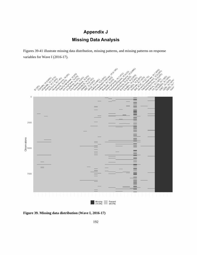
192
Appendix J
Missing Data Analysis
Figures 39-41 illustrate missing data distribution, missing patterns, and missing patterns on response
variables for Wave I (2016-17).
Figure 39. Missing data distribution (Wave I, 2016-17)

193
Figure 40. Missing patterns (Wave I, 2016-17)

194
Figure 41. Missing patterns on response variables (Wave I, 2016-17)

195
Figures 42-44 illustrate missing data distribution, missing patterns, and missing patterns on response
variables for Wave II (2017-18).
Figure 42. Missing data distribution (Wave II, 2017-18)
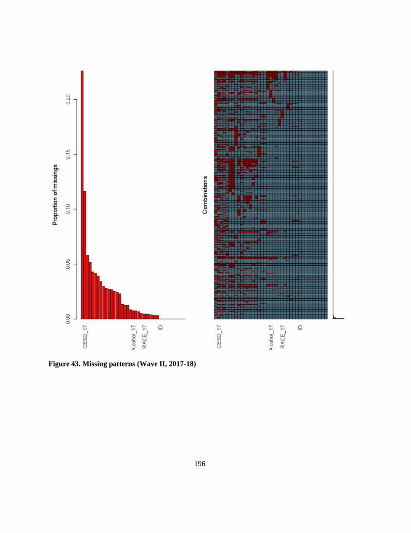
196
Figure 43. Missing patterns (Wave II, 2017-18)
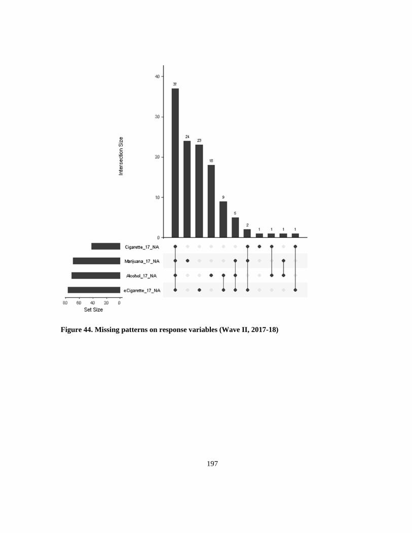
197
Figure 44. Missing patterns on response variables (Wave II, 2017-18)

198
Figures 45-47 illustrate missing data distribution, missing patterns, and missing patterns on response
variables for Wave III (2018-19).
Figure 45. Missing data distribution (Wave III, 2018-19)

199
Figure 46. Missing patterns (Wave III, 2018-19)
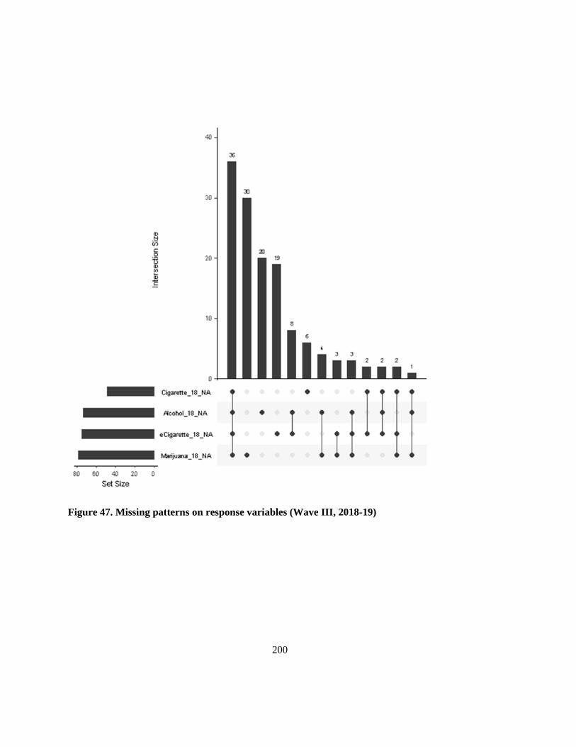
200
Figure 47. Missing patterns on response variables (Wave III, 2018-19)

201
Appendix K
Clustering Results – FCM Clustering
Figures 48-50 illustrate the two-dimensional (2D) representation and the silhouette plot of FCM
clustering on the linked COMPASS data by waves.
Figure 48. FCM Clustering, left-panel: 2D representation; right-panel: silhouette plot (Wave I,
2016-17)
e
Figure 49. FCM Clustering, left-panel: 2D representation; right-panel: silhouette plot (Wave II,
2017-18)
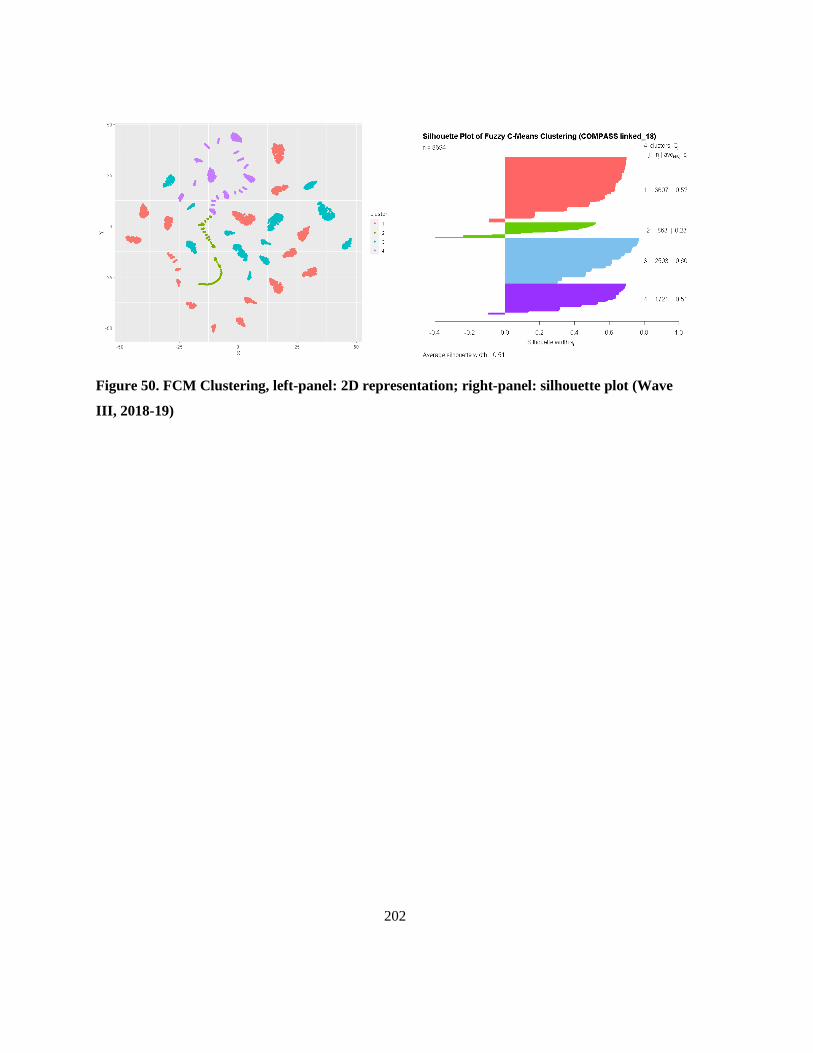
202
Figure 50. FCM Clustering, left-panel: 2D representation; right-panel: silhouette plot (Wave
III, 2018-19)
203
Appendix L
Clustering Results – PAM Clustering
Figures 51-53 illustrate the two-dimensional (2D) representation and the silhouette plot of PAM
clustering on the linked COMPASS data by waves.
Figure 51. PAM Clustering, left-panel: 2D representation; right-panel: silhouette plot (Wave I,
2016-17)
Figure 52. PAM Clustering, left-panel: 2D representation; right-panel: silhouette plot (Wave II,
2017-18)
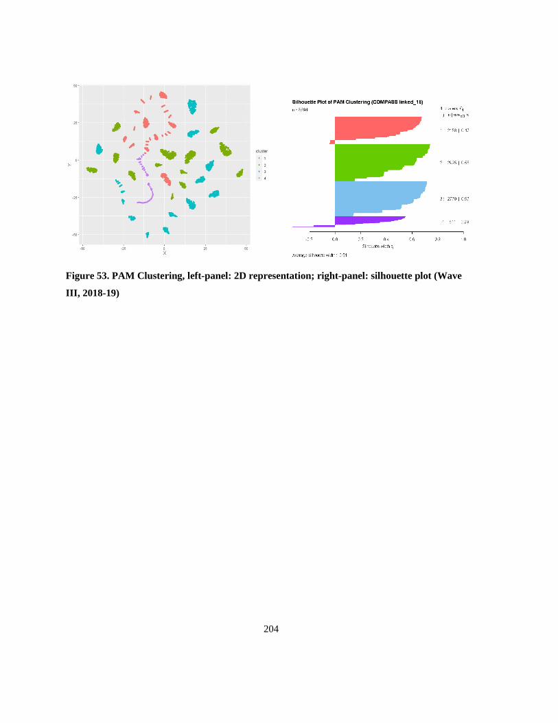
204
Figure 53. PAM Clustering, left-panel: 2D representation; right-panel: silhouette plot (Wave
III, 2018-19)

205
Appendix M
Clustering Results – Hierarchical Clustering
Figures 54, 56, & 58 demonstrate the dendrogram of hierarchical clustering on the linked COMPASS
data by waves. Figures 55, 57, & 59 illustrate the two-dimensional (2D) representation and the
silhouette plot of hierarchical clustering on the linked COMPASS data by waves.
Figure 54. Hierarchical Clustering, Dendrogram (Wave I, 2016-17)

206
Figure 55. Hierarchical Clustering, left-panel: 2D representation; right-panel: silhouette plot
(Wave I, 2016-17)
Figure 56. Hierarchical Clustering, Dendrogram (Wave II, 2017-18)
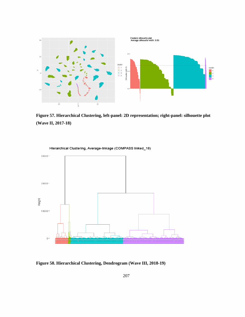
207
Figure 57. Hierarchical Clustering, left-panel: 2D representation; right-panel: silhouette plot
(Wave II, 2017-18)
Figure 58. Hierarchical Clustering, Dendrogram (Wave III, 2018-19)
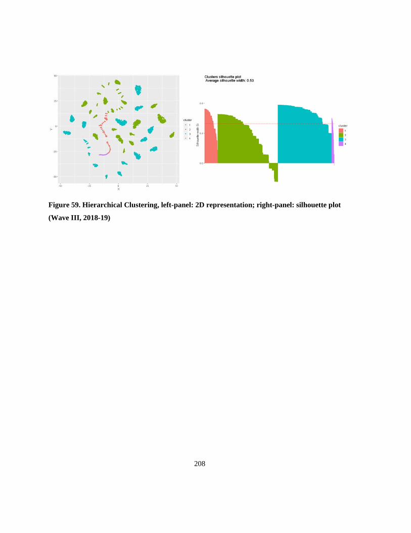
208
Figure 59. Hierarchical Clustering, left-panel: 2D representation; right-panel: silhouette plot
(Wave III, 2018-19)

209
Appendix N
Selection of the Covariates Using LASSO Regression
Tables 26-28 summarize LASSO regression coefficients for all features by waves. Coefficients that
were not shrunk to zero are highlighted in bold font, which was selected for further modelling.
Figures 60-62 illustrate the LASSO coefficients for all features by waves.
Table 26. LASSO coefficients (Wave I, 2016-17)
Number Feature* Coefficient
1 (Intercept) 0.0000
2 HouseholdIncome_16 0.0000
3 Urbanity_16 a -0.0126
4 TotalPointsInterest_16 0.0000
5 DrinkingPlaces_16 0.0000
6 DrugStores_16 0.0000
7 LiquorStores_16 0.0000
8 TobaccoStores_16 0.0000
9 Province_16 a 0.0000
10 Grade_16 a 0.1000
11 Sex_16 0.0000
12 Race_16 a 0.0000
13 GetMoney_16 a 0.0780
14 TransportationToSchool_16 0.0000
15 PAfriends_16 a 0.0000
16 EatingBreakfast_16 a -0.0650
17 SmokingFriends_16 a 0.4925
18 SupportQuitDrugAlcohol_16 a 0.1088
19 EnglishMarks_16 a 0.0194
20 WillingEdu_16 a -0.0269
21 SkipClass_16 a 0.3878
210
Number Feature* Coefficient
22 BMI_CATEGORY_16 a 0.0161
23 SchoolConnectedness_16 a -0.0180
24 SedentaryTime_16 a 0.0003
25 TotalPAtime_16 0.0000
26 PA_LEVEL_16a 0.0000
27 FLOURISH_16 0.0000
28 GAD7_16 a 0.0000
29 CESD_16 a 0.0000
31 DERS_16 a 0.0000
31 GambleOnline_16 a 0.0000
*The last three char “_16” indicates the school year of 2016-17; a see Section 5.4.1 for descriptions
DrinkingPlaces – BE data, counts of drinking places within 1000 meters of schools. Establishments
primarily engaged in the retail sale of alcoholic drinks, such as beer, ale, wine, and liquor, for
consumption on the premises. The sale of food frequently accounts for a substantial portion of the
receipts of these establishments.
FLOURISH – This is a derived variable, scoring from 8 to 40. The higher the score is, the more
psychological resources and strengths are, based on the Flourishing Scale.
HouseholdIncome – SES data, the median total income of households in 2015 ($), categorized into
“25001-50000,” “50001-75000,” “75001-100000,” and “>100000,” dummy coded from 1 to 4,
respectively.
LiquorStores – BE data, counts of liquor stores within 1000 meters of schools. Establishments
primarily engaged in retailing packaged alcoholic beverages, such as ale, beer, wine, and liquor, for
consumption off the premises. Stores selling prepared drinks for consumption on the premises are
classified in Industry 5813.
TobaccoStores – BE data, counts of tobacco stores & stands within 1000 meters of schools.
Establishments primarily engaged in the retail sale of cigarettes, cigars, tobacco, and smokers’
supplies.
TotalPAtime - This is a derived variable, representing total combined HARD and MODERATE
physical activity in minutes, ranging from 0 to 3990.
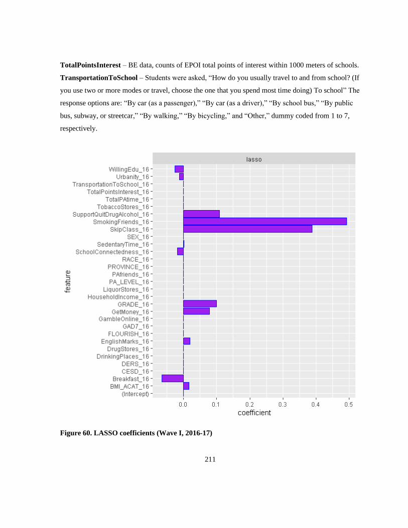
211
TotalPointsInterest – BE data, counts of EPOI total points of interest within 1000 meters of schools.
TransportationToSchool – Students were asked, “How do you usually travel to and from school? (If
you use two or more modes or travel, choose the one that you spend most time doing) To school” The
response options are: “By car (as a passenger),” “By car (as a driver),” “By school bus,” “By public
bus, subway, or streetcar,” “By walking,” “By bicycling,” and “Other,” dummy coded from 1 to 7,
respectively.
Figure 60. LASSO coefficients (Wave I, 2016-17)

212
Table 27. LASSO coefficients (Wave II, 2017-18)
Number Feature* Coefficient
1 (Intercept) 0.0000
2 HouseholdIncome_17 0.0000
3 Urbanity_17 a -0.1336
4 TotalPointsInterest_17 0.0000
5 DrinkingPlaces_17 0.0000
6 DrugStores_17 0.0000
7 LiquorStores_17 0.0000
8 TobaccoStores_17 0.0000
9 Province_17 a 0.0000
10 Grade_17 a 0.0705
11 Sex_17 0.0000
12 Race_17 a -0.0090
13 GetMoney_17 a 0.2031
14 TransportationToSchool_17 0.0000
15 PAfriends_17 a 0.0750
16 EatingBreakfast_17 a -0.2294
17 SmokingFriends_17 a 0.5538
18 SupportQuitDrugAlcohol_17 a 0.1280
19 EnglishMarks_17 a 0.0974
20 WillingEdu_17 a -0.0593
21 SkipClass_17 a 0.4602
22 BMI_CATEGORY_17 a 0.0671
23 SchoolConnectedness_17 a -0.0122
24 SedentaryTime_17 a 0.0003
25 TotalPAtime_17 0.0000
26 PA_LEVEL_17 a 0.0000
27 FLOURISH_17 0.0000
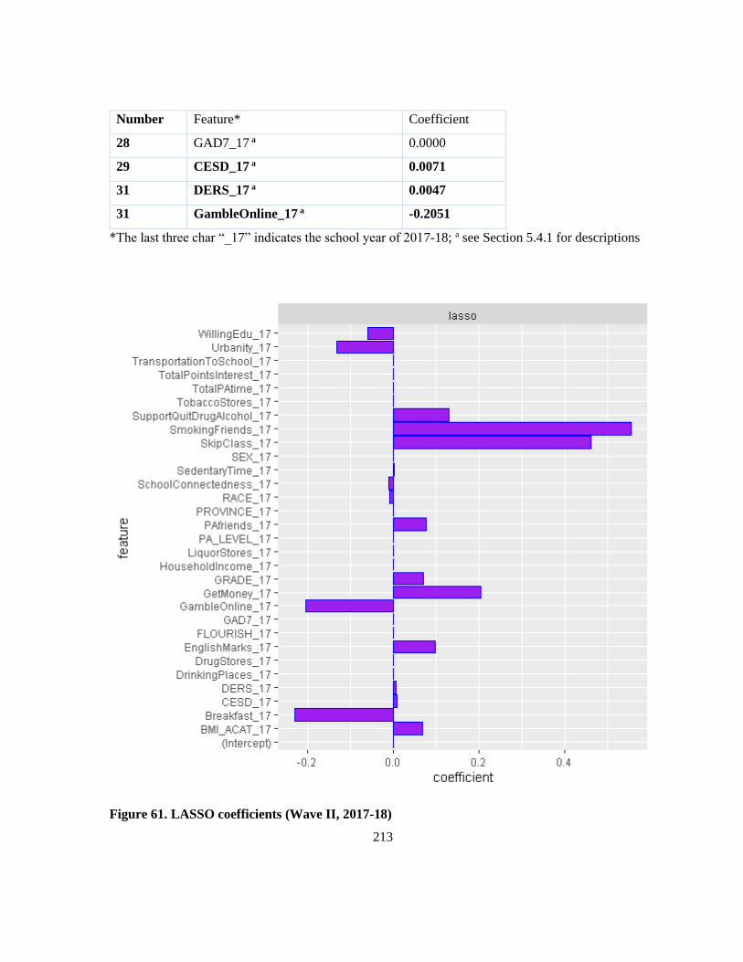
213
Number Feature* Coefficient
28 GAD7_17 a 0.0000
29 CESD_17 a 0.0071
31 DERS_17 a 0.0047
31 GambleOnline_17 a -0.2051
*The last three char “_17” indicates the school year of 2017-18; a see Section 5.4.1 for descriptions
Figure 61. LASSO coefficients (Wave II, 2017-18)

214
Table 28. LASSO coefficients (Wave III, 2018-19)
Number Feature* Coefficient
1 (Intercept) 0.0000
2 HouseholdIncome_18 0.0000
3 Urbanity_18 a -0.1697
4 TotalPointsInterest_18 0.0000
5 DrinkingPlaces_18 0.0000
6 DrugStores_18 -0.0026
7 LiquorStores_18 0.0000
8 TobaccoStores_18 0.0000
9 Province_18 a 0.0000
10 Grade_18 a 0.0238
11 Sex_18 0.0000
12 Race_18 a -0.0387
13 GetMoney_18 a 0.2642
14 TransportationToSchool_18 0.0000
15 PAfriends_18 a 0.1221
16 EatingBreakfast_18 a -0.4282
17 SmokingFriends_18 a 0.5113
18 SupportQuitDrugAlcohol_18 a 0.0569
19 EnglishMarks_18 a 0.1049
20 WillingEdu_18 a -0.0461
21 SkipClass_18 a 0.4876
22 BMI_CATEGORY_18 a 0.0696
23 SchoolConnectedness_18 a -0.0007
24 SedentaryTime_18 a 0.0004
25 TotalPAtime_18 0.0000
26 PA_LEVEL_18 a -0.0240
27 FLOURISH_18 0.0000

215
Number Feature* Coefficient
28 GAD7_18 a 0.0036
29 CESD_18 a 0.0051
31 DERS_18 a 0.0073
31 GambleOnline_18 a -0.1580
*The last three char “_18” indicates the school year of 2018-19; a see Section 5.4.1 for descriptions
Figure 62. LASSO coefficients (Wave III, 2018-19)

216
Appendix O
Definition of urban/rural classification11
Large Urban Populations from ≥100,000 and a population density of at least 400 per square
kilometre
Medium
Urban
Populations between 30,000 to 99,999 and a population density of at least 400
per square kilometre
Small Urban Populations between 1,000 to 29,999 and a population density of at least 400
per square kilometre
Rural Population less than 1,000 or population density less than 400 per square
kilometre
11 Source: Dictionary, Census of Population, 2016, Population Centre (POPCTR)
https://www12.statcan.gc.ca/census-recensement/2016/ref/dict/geo049a-eng.cfm
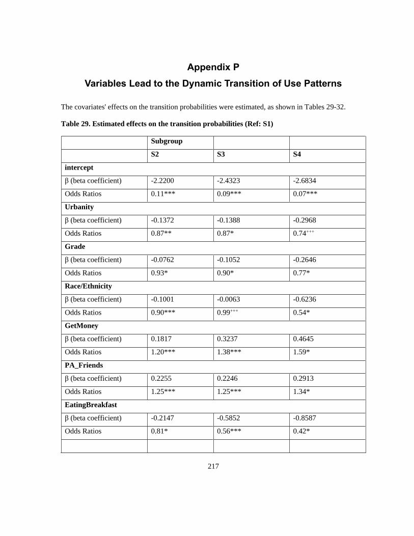
217
Appendix P
Variables Lead to the Dynamic Transition of Use Patterns
The covariates' effects on the transition probabilities were estimated, as shown in Tables 29-32.
Table 29. Estimated effects on the transition probabilities (Ref: S1)
Subgroup
S2 S3 S4
intercept
β (beta coefficient) -2.2200 -2.4323 -2.6834
Odds Ratios 0.11*** 0.09*** 0.07***
Urbanity
β (beta coefficient) -0.1372 -0.1388 -0.2968
Odds Ratios 0.87** 0.87* 0.74+++
Grade
β (beta coefficient) -0.0762 -0.1052 -0.2646
Odds Ratios 0.93* 0.90* 0.77*
Race/Ethnicity
β (beta coefficient) -0.1001 -0.0063 -0.6236
Odds Ratios 0.90*** 0.99+++ 0.54*
GetMoney
β (beta coefficient) 0.1817 0.3237 0.4645
Odds Ratios 1.20*** 1.38*** 1.59*
PA_Friends
β (beta coefficient) 0.2255 0.2246 0.2913
Odds Ratios 1.25*** 1.25*** 1.34*
EatingBreakfast
β (beta coefficient) -0.2147 -0.5852 -0.8587
Odds Ratios 0.81* 0.56*** 0.42*
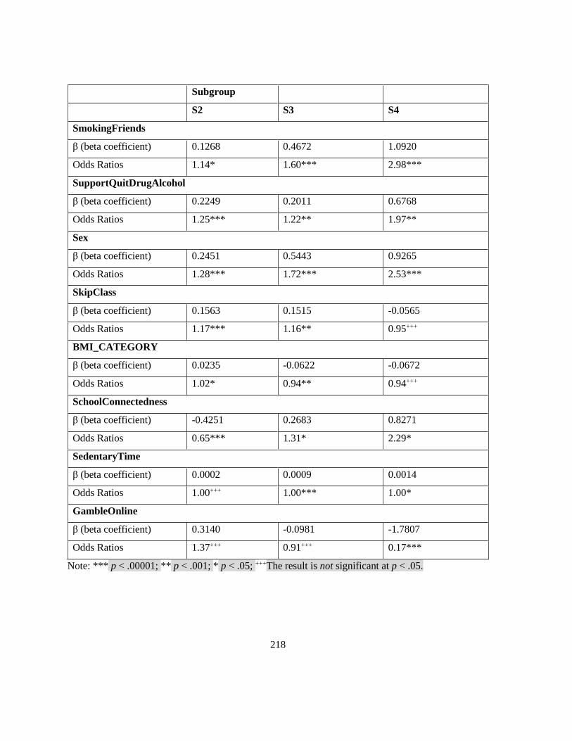
218
Subgroup
S2 S3 S4
SmokingFriends
β (beta coefficient) 0.1268 0.4672 1.0920
Odds Ratios 1.14* 1.60*** 2.98***
SupportQuitDrugAlcohol
β (beta coefficient) 0.2249 0.2011 0.6768
Odds Ratios 1.25*** 1.22** 1.97**
Sex
β (beta coefficient) 0.2451 0.5443 0.9265
Odds Ratios 1.28*** 1.72*** 2.53***
SkipClass
β (beta coefficient) 0.1563 0.1515 -0.0565
Odds Ratios 1.17*** 1.16** 0.95+++
BMI_CATEGORY
β (beta coefficient) 0.0235 -0.0622 -0.0672
Odds Ratios 1.02* 0.94** 0.94+++
SchoolConnectedness
β (beta coefficient) -0.4251 0.2683 0.8271
Odds Ratios 0.65*** 1.31* 2.29*
SedentaryTime
β (beta coefficient) 0.0002 0.0009 0.0014
Odds Ratios 1.00+++ 1.00*** 1.00*
GambleOnline
β (beta coefficient) 0.3140 -0.0981 -1.7807
Odds Ratios 1.37+++ 0.91+++ 0.17***
Note: *** p < .00001; ** p < .001; * p < .05; +++The result is not significant at p < .05.

219
Table 30. Estimated effects on the transition probabilities (Ref: S2)
Subgroup
S1 S3 S4
intercept
β (beta coefficient) -2.1540 -2.0710 -2.1830
Odds Ratios 0.12*** 0.13*** 0.11***
Urbanity
β (beta coefficient) 1.6465 -0.0724 0.1817
Odds Ratios 5.19*** 0.93+++ 1.20+++
Grade
β (beta coefficient) -0.3805 -0.0682 -0.4207
Odds Ratios 0.68* 0.93+++ 0.66*
Race/Ethnicity
β (beta coefficient) 0.5650 -0.0325 -0.0636
Odds Ratios 1.76* 0.97+++ 0.94+++
GetMoney
β (beta coefficient) -0.5312 0.1749 0.2594
Odds Ratios 0.59+++ 1.19*** 1.30+++
PA_Friends
β (beta coefficient) -1.1226 0.2104 -0.0643
Odds Ratios 0.33*** 1.23*** 0.94+++
EatingBreakfast
β (beta coefficient) 0.4412 -0.3779 -0.0386
Odds Ratios 1.55*** 0.69** 0.96+++
SmokingFriends
β (beta coefficient) -0.6685 0.3290 1.0821
Odds Ratios 0.51*** 1.39** 2.95***
SupportQuitDrugAlcohol
β (beta coefficient) 1.7343 0.1345 0.4364
Odds Ratios 5.67*** 1.14* 1.55*

220
Subgroup
S1 S3 S4
Sex
β (beta coefficient) -0.4571 0.3200 0.8886
Odds Ratios 0.63*** 1.38*** 2.43***
SkipClass
β (beta coefficient) -1.2956 -0.0010 0.1493
Odds Ratios 0.27** 1.00+++ 1.16+++
BMI_CATEGORY
β (beta coefficient) -0.3804 0.0027 -0.1336
Odds Ratios 0.68* 1.00+++ 0.88*
SchoolConnectedness
β (beta coefficient) 0.8150 0.0996 -1.7318
Odds Ratios 2.26*** 1.10+++ 0.18***
SedentaryTime
β (beta coefficient) -0.0070 0.0008 0.0014
Odds Ratios 0.99* 1.00** 1.00*
GambleOnline
β (beta coefficient) 0.3639 0.2774 1.2055
Odds Ratios 1.44*** 1.32+++ 3.34***
Note: *** p < .00001; ** p < .001; * p < .05; +++The result is not significant at p < .05.
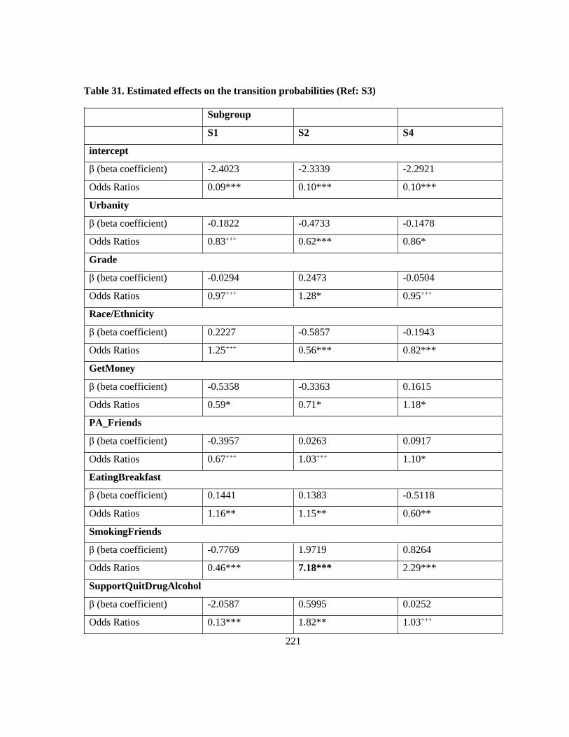
221
Table 31. Estimated effects on the transition probabilities (Ref: S3)
Subgroup
S1 S2 S4
intercept
β (beta coefficient) -2.4023 -2.3339 -2.2921
Odds Ratios 0.09*** 0.10*** 0.10***
Urbanity
β (beta coefficient) -0.1822 -0.4733 -0.1478
Odds Ratios 0.83+++ 0.62*** 0.86*
Grade
β (beta coefficient) -0.0294 0.2473 -0.0504
Odds Ratios 0.97+++ 1.28* 0.95+++
Race/Ethnicity
β (beta coefficient) 0.2227 -0.5857 -0.1943
Odds Ratios 1.25+++ 0.56*** 0.82***
GetMoney
β (beta coefficient) -0.5358 -0.3363 0.1615
Odds Ratios 0.59* 0.71* 1.18*
PA_Friends
β (beta coefficient) -0.3957 0.0263 0.0917
Odds Ratios 0.67+++ 1.03+++ 1.10*
EatingBreakfast
β (beta coefficient) 0.1441 0.1383 -0.5118
Odds Ratios 1.16** 1.15** 0.60**
SmokingFriends
β (beta coefficient) -0.7769 1.9719 0.8264
Odds Ratios 0.46*** 7.18*** 2.29***
SupportQuitDrugAlcohol
β (beta coefficient) -2.0587 0.5995 0.0252
Odds Ratios 0.13*** 1.82** 1.03+++

222
Subgroup
S1 S2 S4
Sex
β (beta coefficient) -1.0160 -0.6422 0.4037
Odds Ratios 0.36*** 0.53*** 1.50***
SkipClass
β (beta coefficient) -1.2329 -1.3169 0.0608
Odds Ratios 0.29*** 0.27*** 1.06+++
BMI_CATEGORY
β (beta coefficient) 0.3661 -0.3142 -0.0467
Odds Ratios 1.44** 0.73* 0.95*
SchoolConnectedness
β (beta coefficient) 0.5030 0.2629 0.5969
Odds Ratios 1.65*** 1.30*** 1.82***
SedentaryTime
β (beta coefficient) -0.0027 -0.0069 0.0008
Odds Ratios 1.00+++ 0.99+++ 1.00**
GambleOnline
β (beta coefficient) -0.3335 -0.3544 0.3193
Odds Ratios 0.72*** 0.70*** 1.38+++
Note: *** p < .00001; ** p < .001; * p < .05; +++The result is not significant at p < .05.
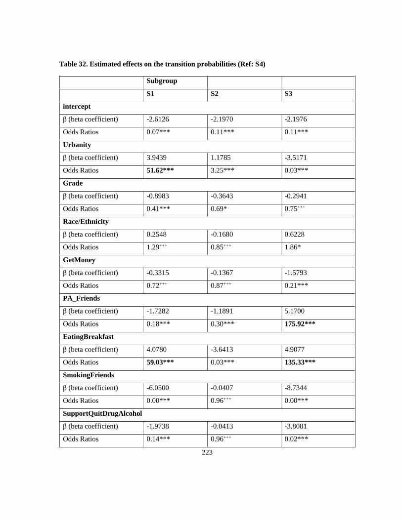
223
Table 32. Estimated effects on the transition probabilities (Ref: S4)
Subgroup
S1 S2 S3
intercept
β (beta coefficient) -2.6126 -2.1970 -2.1976
Odds Ratios 0.07*** 0.11*** 0.11***
Urbanity
β (beta coefficient) 3.9439 1.1785 -3.5171
Odds Ratios 51.62*** 3.25*** 0.03***
Grade
β (beta coefficient) -0.8983 -0.3643 -0.2941
Odds Ratios 0.41*** 0.69* 0.75+++
Race/Ethnicity
β (beta coefficient) 0.2548 -0.1680 0.6228
Odds Ratios 1.29+++ 0.85+++ 1.86*
GetMoney
β (beta coefficient) -0.3315 -0.1367 -1.5793
Odds Ratios 0.72+++ 0.87+++ 0.21***
PA_Friends
β (beta coefficient) -1.7282 -1.1891 5.1700
Odds Ratios 0.18*** 0.30*** 175.92***
EatingBreakfast
β (beta coefficient) 4.0780 -3.6413 4.9077
Odds Ratios 59.03*** 0.03*** 135.33***
SmokingFriends
β (beta coefficient) -6.0500 -0.0407 -8.7344
Odds Ratios 0.00*** 0.96+++ 0.00***
SupportQuitDrugAlcohol
β (beta coefficient) -1.9738 -0.0413 -3.8081
Odds Ratios 0.14*** 0.96+++ 0.02***

224
Subgroup
S1 S2 S3
Sex
β (beta coefficient) -7.2141 -0.0427 -2.8812
Odds Ratios 0.00*** 0.96+++ 0.06***
SkipClass
β (beta coefficient) -0.3462 -3.9090 4.5949
Odds Ratios 0.71* 0.02*** 98.97***
BMI_CATEGORY
β (beta coefficient) 0.1361 0.2995 0.0328
Odds Ratios 1.15+++ 1.35* 1.03+++
SchoolConnectedness
β (beta coefficient) 5.7045 -3.0077 -0.7665
Odds Ratios 300.22*** 0.05*** 0.46***
SedentaryTime
β (beta coefficient) -0.0048 -0.0001 0.0058
Odds Ratios 1.00* 1.00+++ 1.01***
GambleOnline
β (beta coefficient) -0.3883 0.0197 -6.7661
Odds Ratios 0.68*** 1.02+++ 0.00***
Note: *** p < .00001; ** p < .001; * p < .05; +++The result is not significant at p < .05.
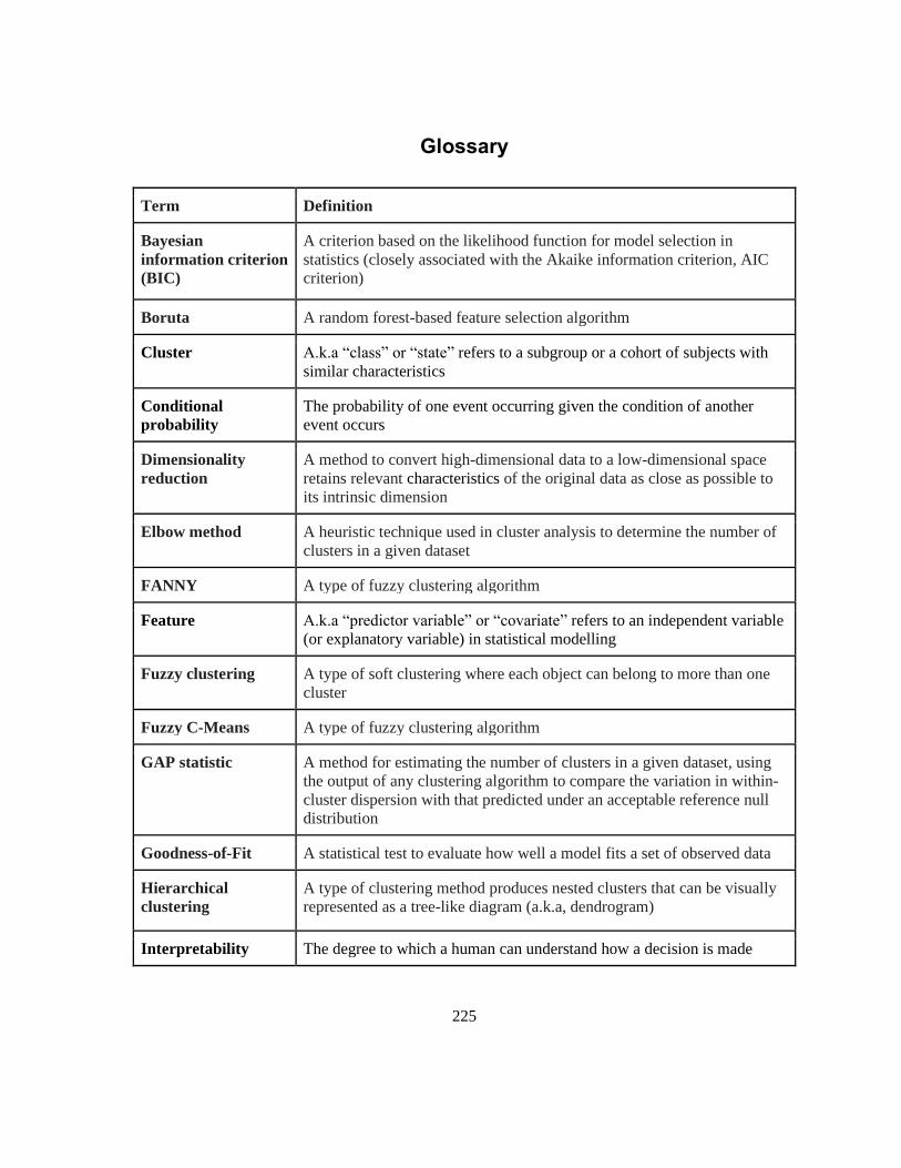
225
Glossary
Term Definition
Bayesian
information criterion
(BIC)
A criterion based on the likelihood function for model selection in
statistics (closely associated with the Akaike information criterion, AIC
criterion)
Boruta A random forest-based feature selection algorithm
Cluster A.k.a “class” or “state” refers to a subgroup or a cohort of subjects with
similar characteristics
Conditional
probability
The probability of one event occurring given the condition of another
event occurs
Dimensionality
reduction
A method to convert high-dimensional data to a low-dimensional space
retains relevant characteristics of the original data as close as possible to
its intrinsic dimension
Elbow method A heuristic technique used in cluster analysis to determine the number of
clusters in a given dataset
FANNY A type of fuzzy clustering algorithm
Feature A.k.a “predictor variable” or “covariate” refers to an independent variable
(or explanatory variable) in statistical modelling
Fuzzy clustering A type of soft clustering where each object can belong to more than one
cluster
Fuzzy C-Means A type of fuzzy clustering algorithm
GAP statistic A method for estimating the number of clusters in a given dataset, using
the output of any clustering algorithm to compare the variation in within-
cluster dispersion with that predicted under an acceptable reference null
distribution
Goodness-of-Fit A statistical test to evaluate how well a model fits a set of observed data
Hierarchical
clustering
A type of clustering method produces nested clusters that can be visually
represented as a tree-like diagram (a.k.a, dendrogram)
Interpretability The degree to which a human can understand how a decision is made
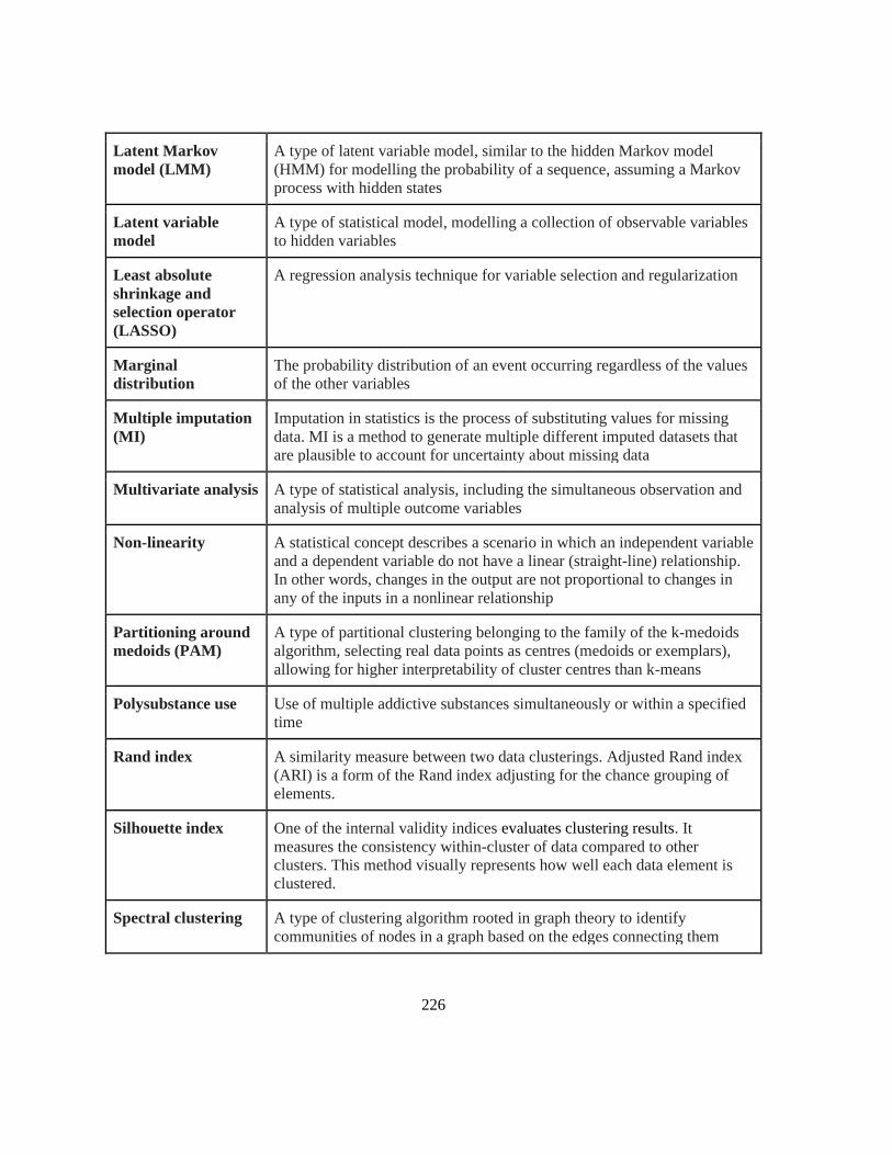
226
Latent Markov
model (LMM)
A type of latent variable model, similar to the hidden Markov model
(HMM) for modelling the probability of a sequence, assuming a Markov
process with hidden states
Latent variable
model
A type of statistical model, modelling a collection of observable variables
to hidden variables
Least absolute
shrinkage and
selection operator
(LASSO)
A regression analysis technique for variable selection and regularization
Marginal
distribution
The probability distribution of an event occurring regardless of the values
of the other variables
Multiple imputation
(MI)
Imputation in statistics is the process of substituting values for missing
data. MI is a method to generate multiple different imputed datasets that
are plausible to account for uncertainty about missing data
Multivariate analysis A type of statistical analysis, including the simultaneous observation and
analysis of multiple outcome variables
Non-linearity A statistical concept describes a scenario in which an independent variable
and a dependent variable do not have a linear (straight-line) relationship.
In other words, changes in the output are not proportional to changes in
any of the inputs in a nonlinear relationship
Partitioning around
medoids (PAM)
A type of partitional clustering belonging to the family of the k-medoids
algorithm, selecting real data points as centres (medoids or exemplars),
allowing for higher interpretability of cluster centres than k-means
Polysubstance use Use of multiple addictive substances simultaneously or within a specified
time
Rand index A similarity measure between two data clusterings. Adjusted Rand index
(ARI) is a form of the Rand index adjusting for the chance grouping of
elements.
Silhouette index One of the internal validity indices evaluates clustering results. It
measures the consistency within-cluster of data compared to other
clusters. This method visually represents how well each data element is
clustered.
Spectral clustering A type of clustering algorithm rooted in graph theory to identify
communities of nodes in a graph based on the edges connecting them

227
t-Distributed
Stochastic Neighbor
Embedding (t-SNE)
A non-linear machine learning algorithm for reducing dimensionality and
visually presenting high-dimensional data