DDOS DETECTION MODELS USING MACHINE AND DEEP ...

DDOS DETECTION MODELS USING MACHINE AND DEEP LEARNINGALGORITHMS AND DISTRIBUTED SYSTEMS

by

Amjad Alsirhani

Submitted in partial fulfillment of the requirementsfor the degree of Doctor of Philosophy

at

Dalhousie UniversityHalifax, Nova Scotia

December 2019

© Copyright by Amjad Alsirhani, 2019

Dedication

This thesis is dedicated to my beloved

Mother and late Father

&

Wife and Children

&

Family

ii

Table of Contents

List of Tables . . . . . . . . . . . . . . . . . . . . . . . . . . . . . . . . . . . . . . . . . . . viii

List of Figures . . . . . . . . . . . . . . . . . . . . . . . . . . . . . . . . . . . . . . . . . . . x

Abstract . . . . . . . . . . . . . . . . . . . . . . . . . . . . . . . . . . . . . . . . . . . . . . xiii

List of Abbreviations and Symbols Used . . . . . . . . . . . . . . . . . . . . . . . . . . . xiv

Acknowledgements . . . . . . . . . . . . . . . . . . . . . . . . . . . . . . . . . . . . . . . . xviii

Chapter 1 Introduction . . . . . . . . . . . . . . . . . . . . . . . . . . . . . . . . . . 1

1.1 Overview and Motivation . . . . . . . . . . . . . . . . . . . . . . . . . . . . . . . . 1

1.2 Thesis Objectives . . . . . . . . . . . . . . . . . . . . . . . . . . . . . . . . . . . . 6

1.3 Research Questions . . . . . . . . . . . . . . . . . . . . . . . . . . . . . . . . . . . 6

1.4 Thesis Contributions . . . . . . . . . . . . . . . . . . . . . . . . . . . . . . . . . . 6

1.5 Thesis Outline . . . . . . . . . . . . . . . . . . . . . . . . . . . . . . . . . . . . . . 10

Chapter 2 Literature Survey and Background . . . . . . . . . . . . . . . . . . . . . 11

2.1 Overview . . . . . . . . . . . . . . . . . . . . . . . . . . . . . . . . . . . . . . . . . 11

2.2 DDoS Attacks . . . . . . . . . . . . . . . . . . . . . . . . . . . . . . . . . . . . . . 11

2.3 How a DDoS Can be Launched . . . . . . . . . . . . . . . . . . . . . . . . . . . . . 11

2.4 Types of DDoS Attacks . . . . . . . . . . . . . . . . . . . . . . . . . . . . . . . . . 12

2.5 DDoS Detection Approaches . . . . . . . . . . . . . . . . . . . . . . . . . . . . . . 13

2.5.1 Machine Learning Approaches . . . . . . . . . . . . . . . . . . . . . . . . 14

2.5.2 Deep Learning Approaches . . . . . . . . . . . . . . . . . . . . . . . . . . 16

2.5.3 Distributed System Approaches . . . . . . . . . . . . . . . . . . . . . . . . 17

iii

Chapter 3 Distributed System, Dataset, and Evaluation Measurements . . . . . . 19

3.1 Overview . . . . . . . . . . . . . . . . . . . . . . . . . . . . . . . . . . . . . . . . . 19

3.2 Distributed System . . . . . . . . . . . . . . . . . . . . . . . . . . . . . . . . . . . 19

3.3 Apache Spark . . . . . . . . . . . . . . . . . . . . . . . . . . . . . . . . . . . . . . 193.3.1 Spark Overview . . . . . . . . . . . . . . . . . . . . . . . . . . . . . . . . . 193.3.2 Spark Architecture . . . . . . . . . . . . . . . . . . . . . . . . . . . . . . . 20

3.4 Apache Hadoop . . . . . . . . . . . . . . . . . . . . . . . . . . . . . . . . . . . . . 223.4.1 Hadoop Overview . . . . . . . . . . . . . . . . . . . . . . . . . . . . . . . . 223.4.2 Hadoop YARN . . . . . . . . . . . . . . . . . . . . . . . . . . . . . . . . . . 23

3.5 Dataset . . . . . . . . . . . . . . . . . . . . . . . . . . . . . . . . . . . . . . . . . . 24

3.6 Evaluation Method . . . . . . . . . . . . . . . . . . . . . . . . . . . . . . . . . . . 25

Chapter 4 DDoS Detection System Based on a Gradient Boosting Algorithm and aDistributed System . . . . . . . . . . . . . . . . . . . . . . . . . . . . . . 29

4.1 Overview . . . . . . . . . . . . . . . . . . . . . . . . . . . . . . . . . . . . . . . . . 29

4.2 Motivations and Objectives . . . . . . . . . . . . . . . . . . . . . . . . . . . . . . . 29

4.3 Literature Review . . . . . . . . . . . . . . . . . . . . . . . . . . . . . . . . . . . . 30

4.4 Methodology and System Design . . . . . . . . . . . . . . . . . . . . . . . . . . . 324.4.1 Overview . . . . . . . . . . . . . . . . . . . . . . . . . . . . . . . . . . . . . 324.4.2 Gradient Boosting Algorithm . . . . . . . . . . . . . . . . . . . . . . . . . 324.4.3 Network Analysis Tool and Software . . . . . . . . . . . . . . . . . . . . . 34

4.5 Evaluation . . . . . . . . . . . . . . . . . . . . . . . . . . . . . . . . . . . . . . . . 344.5.1 Experimental Settings . . . . . . . . . . . . . . . . . . . . . . . . . . . . . 344.5.2 Evaluation Method . . . . . . . . . . . . . . . . . . . . . . . . . . . . . . . 35

4.6 Results . . . . . . . . . . . . . . . . . . . . . . . . . . . . . . . . . . . . . . . . . . 364.6.1 GBT Algorithm Performance Rates and Delays for both Datasets . . . . . 364.6.2 GBT Performance when Varying Iterations and Decision Tree Depth . . . 38

4.7 Chapter Conclusion . . . . . . . . . . . . . . . . . . . . . . . . . . . . . . . . . . . 41

iv

Chapter 5 Dynamic Model Selection Using Fuzzy Logic System . . . . . . . . . . 42

5.1 Overview . . . . . . . . . . . . . . . . . . . . . . . . . . . . . . . . . . . . . . . . . 42


5.3 Chapter Contributions . . . . . . . . . . . . . . . . . . . . . . . . . . . . . . . . . 44

5.4 Methodology and System Design . . . . . . . . . . . . . . . . . . . . . . . . . . . 455.4.1 Overview . . . . . . . . . . . . . . . . . . . . . . . . . . . . . . . . . . . . . 455.4.2 System Workflow . . . . . . . . . . . . . . . . . . . . . . . . . . . . . . . . 465.4.3 Classification Algorithms . . . . . . . . . . . . . . . . . . . . . . . . . . . 475.4.4 Fuzzy Logic System . . . . . . . . . . . . . . . . . . . . . . . . . . . . . . . 49

5.5 Evaluation . . . . . . . . . . . . . . . . . . . . . . . . . . . . . . . . . . . . . . . . 525.5.1 Evaluation Method . . . . . . . . . . . . . . . . . . . . . . . . . . . . . . . 525.5.2 Network Analysis Tool and Software . . . . . . . . . . . . . . . . . . . . . 525.5.3 Implementation and Configuration of the Prototype . . . . . . . . . . . . 53

5.6 Results . . . . . . . . . . . . . . . . . . . . . . . . . . . . . . . . . . . . . . . . . . 535.6.1 Classification Algorithms Performance Measurements . . . . . . . . . . . 535.6.2 Classification Algorithms Performance Results . . . . . . . . . . . . . . . 535.6.3 Analysis of the Distributed System . . . . . . . . . . . . . . . . . . . . . . 555.6.4 Analysis of Fuzzy Logic System . . . . . . . . . . . . . . . . . . . . . . . . 62

5.7 Discussion . . . . . . . . . . . . . . . . . . . . . . . . . . . . . . . . . . . . . . . . 695.7.1 Classification Algorithms . . . . . . . . . . . . . . . . . . . . . . . . . . . 705.7.2 Distributed System . . . . . . . . . . . . . . . . . . . . . . . . . . . . . . . 705.7.3 Fuzzy Logic System . . . . . . . . . . . . . . . . . . . . . . . . . . . . . . . 71


5.9 Limitations and Future Work . . . . . . . . . . . . . . . . . . . . . . . . . . . . . 72

Chapter 6 Features Selection Framework Based on Chi-Square Algorithm . . . . 73

6.1 Overview . . . . . . . . . . . . . . . . . . . . . . . . . . . . . . . . . . . . . . . . . 73

6.2 Motivations and Objectives . . . . . . . . . . . . . . . . . . . . . . . . . . . . . . . 736.2.1 Motivation . . . . . . . . . . . . . . . . . . . . . . . . . . . . . . . . . . . . 736.2.2 Objective . . . . . . . . . . . . . . . . . . . . . . . . . . . . . . . . . . . . . 74

v

6.3 Literature Review . . . . . . . . . . . . . . . . . . . . . . . . . . . . . . . . . . . . 746.3.1 Background . . . . . . . . . . . . . . . . . . . . . . . . . . . . . . . . . . . 746.3.2 Literature Review . . . . . . . . . . . . . . . . . . . . . . . . . . . . . . . . 75

6.4 System Architecture . . . . . . . . . . . . . . . . . . . . . . . . . . . . . . . . . . 776.4.1 Overview . . . . . . . . . . . . . . . . . . . . . . . . . . . . . . . . . . . . . 776.4.2 Chi-Square feature selection approaches . . . . . . . . . . . . . . . . . . . 77

6.5 Evaluation . . . . . . . . . . . . . . . . . . . . . . . . . . . . . . . . . . . . . . . . 806.5.1 Experimental Settings . . . . . . . . . . . . . . . . . . . . . . . . . . . . . 806.5.2 Evaluation Method . . . . . . . . . . . . . . . . . . . . . . . . . . . . . . . 806.5.3 Analysis of the Feature Selection Algorithms’ Performance . . . . . . . . 816.5.4 Classifiers’ Training and Feature Selection (FS) Processing Delays . . . . 836.5.5 Classifiers’ Performance . . . . . . . . . . . . . . . . . . . . . . . . . . . . 87

6.6 Discussion . . . . . . . . . . . . . . . . . . . . . . . . . . . . . . . . . . . . . . . . 90



Chapter 7 DDoSDetection FrameworkUsingDeep Learning and aDistributed Sys-tem . . . . . . . . . . . . . . . . . . . . . . . . . . . . . . . . . . . . . . . . 92

7.1 Overview . . . . . . . . . . . . . . . . . . . . . . . . . . . . . . . . . . . . . . . . . 92


7.3 Literature Review . . . . . . . . . . . . . . . . . . . . . . . . . . . . . . . . . . . . 94

7.4 Chapter Contributions . . . . . . . . . . . . . . . . . . . . . . . . . . . . . . . . . 96

7.5 Methodology . . . . . . . . . . . . . . . . . . . . . . . . . . . . . . . . . . . . . . . 967.5.1 Overview . . . . . . . . . . . . . . . . . . . . . . . . . . . . . . . . . . . . . 967.5.2 Deep Learning Application to DDoS Filtering . . . . . . . . . . . . . . . . 97

7.6 Experiments and Evaluation . . . . . . . . . . . . . . . . . . . . . . . . . . . . . . 997.6.1 Evaluation Methods . . . . . . . . . . . . . . . . . . . . . . . . . . . . . . . 997.6.2 Experimental Settings . . . . . . . . . . . . . . . . . . . . . . . . . . . . . 997.6.3 Dataset . . . . . . . . . . . . . . . . . . . . . . . . . . . . . . . . . . . . . . 997.6.4 Deep Learning Model Architecture . . . . . . . . . . . . . . . . . . . . . . 101

vi

7.6.5 Performance Measurements . . . . . . . . . . . . . . . . . . . . . . . . . . 102

7.7 Results . . . . . . . . . . . . . . . . . . . . . . . . . . . . . . . . . . . . . . . . . . 1027.7.1 Neural Network Performance . . . . . . . . . . . . . . . . . . . . . . . . . 1027.7.2 Classifier in ROC . . . . . . . . . . . . . . . . . . . . . . . . . . . . . . . . 1037.7.3 Training Time and Testing Time analysis . . . . . . . . . . . . . . . . . . . 103

7.8 Discussion . . . . . . . . . . . . . . . . . . . . . . . . . . . . . . . . . . . . . . . . 104



Chapter 8 Conclusion and Future Work . . . . . . . . . . . . . . . . . . . . . . . . . 108

8.1 Conclusion . . . . . . . . . . . . . . . . . . . . . . . . . . . . . . . . . . . . . . . . 108

8.2 Future Work . . . . . . . . . . . . . . . . . . . . . . . . . . . . . . . . . . . . . . . 1098.2.1 Future Directions . . . . . . . . . . . . . . . . . . . . . . . . . . . . . . . . 1098.2.2 Extending Work on Frameworks . . . . . . . . . . . . . . . . . . . . . . . 111

Bibliography . . . . . . . . . . . . . . . . . . . . . . . . . . . . . . . . . . . . . . . . . . . . 112

Appendix Appendix A . . . . . . . . . . . . . . . . . . . . . . . . . . . . . . . . . . . . 121

A.1 Spark and Hadoop configuration . . . . . . . . . . . . . . . . . . . . . . . . . . . 121A.1.1 Java Installation . . . . . . . . . . . . . . . . . . . . . . . . . . . . . . . . . 121A.1.2 Spark Installation . . . . . . . . . . . . . . . . . . . . . . . . . . . . . . . . 121A.1.3 Spark Configurations . . . . . . . . . . . . . . . . . . . . . . . . . . . . . . 122A.1.4 Spark files system configuration . . . . . . . . . . . . . . . . . . . . . . . . 123A.1.5 Maven Installation and Configurations . . . . . . . . . . . . . . . . . . . . 126A.1.6 Open ssh-server Configurations . . . . . . . . . . . . . . . . . . . . . . . . 127A.1.7 Spark Initializations . . . . . . . . . . . . . . . . . . . . . . . . . . . . . . 128A.1.8 Hadoop Initializations . . . . . . . . . . . . . . . . . . . . . . . . . . . . . 129A.1.9 Spark application submission . . . . . . . . . . . . . . . . . . . . . . . . . 130

A.2 Neural Network Performance . . . . . . . . . . . . . . . . . . . . . . . . . . . . . 131

A.3 List of Publications . . . . . . . . . . . . . . . . . . . . . . . . . . . . . . . . . . . 138

A.4 Copyright Permission Letters . . . . . . . . . . . . . . . . . . . . . . . . . . . . . 139

vii

List of Tables

1.1 Number of DDoS attacks that have been launched in the last decade witha high impact . . . . . . . . . . . . . . . . . . . . . . . . . . . . . . . . . . . 5

3.1 Extracted feature from the original packets . . . . . . . . . . . . . . . . . . 25

3.2 Features based on their category . . . . . . . . . . . . . . . . . . . . . . . . 25

3.3 Extracted features from the packets to form a small dataset . . . . . . . . . 26

3.4 Confusion matrix . . . . . . . . . . . . . . . . . . . . . . . . . . . . . . . . . 26

4.1 Performance rates and the delays for the Dataset 1 with number of iterationequal to 1 . . . . . . . . . . . . . . . . . . . . . . . . . . . . . . . . . . . . . 36






5.1 Performance rates for classification algorithms for Dataset1 and Dataset2for 100K packets . . . . . . . . . . . . . . . . . . . . . . . . . . . . . . . . . 54

5.2 Performance rates for classification algorithms for Dataset1 and Dataset2for 500K packets . . . . . . . . . . . . . . . . . . . . . . . . . . . . . . . . . 54

5.3 Performance rates for classification algorithms for Dataset1 and Dataset2for one million packets . . . . . . . . . . . . . . . . . . . . . . . . . . . . . . 54

viii

5.4 Performance rates for classification algorithms for Dataset1 and Dataset2for two millions packets . . . . . . . . . . . . . . . . . . . . . . . . . . . . . 55

5.5 Comparison delays for classification algorithms for different sizes of Dataset1and Dataset2 in millisecond in different number of nodes . . . . . . . . . 57

5.6 Comparison delays for classification algorithms for different sizes of Dataset1and Dataset2 in millisecond in different number of nodes . . . . . . . . . 58

5.7 Rules of members in which the traffic volume is High . . . . . . . . . . . . 63

5.8 Rules of members in which the traffic volume is Medium . . . . . . . . . . 64

6.1 Chi-Square test table to calculate the χ2 score of a feature X . . . . . . . . 78

6.2 Extracted feature from the original packets . . . . . . . . . . . . . . . . . . 81

6.3 Selected features, for the dataset size 100K, based on Chi-Square variantspresented by their index from table 6.2 . . . . . . . . . . . . . . . . . . . . 82

6.4 Selected features, for the dataset size 500K, based on Chi-Square variantspresented by their index from table 6.2 . . . . . . . . . . . . . . . . . . . . 82

6.5 Selected features, for the dataset size 1M, based on Chi-Square variantspresented by their index from table 6.2 . . . . . . . . . . . . . . . . . . . . 82

6.6 Selected features, for the dataset 2 M, based on Chi-Square variants pre-sented by their index from table 6.2 . . . . . . . . . . . . . . . . . . . . . . 83

6.7 Classifiers’ training times and the Chi-Square variants processing delaysand their totals of 100K and 500K sample sizes reported in (ms) . . . . . . 84

6.8 Classifiers’ training times and the Chi-Square variants processing delaysand their totals of 1M and 2M sample sizes reported in (ms) . . . . . . . . 85

6.9 Performance rates for classification algorithms for different sizes of in-stance from Chi-Square variants . . . . . . . . . . . . . . . . . . . . . . . . 89

7.1 Dataset sizes and class imbalance . . . . . . . . . . . . . . . . . . . . . . . . 100

7.2 Training time in seconds . . . . . . . . . . . . . . . . . . . . . . . . . . . . . 103

7.3 Prediction time in seconds . . . . . . . . . . . . . . . . . . . . . . . . . . . . 105

ix

List of Figures

1.1 Digital Attack Map (Top daily DDoS attack worldwide) . . . . . . . . . . 2

1.2 Thesis Contributions . . . . . . . . . . . . . . . . . . . . . . . . . . . . . . 9

2.1 Example of DDoS attacks . . . . . . . . . . . . . . . . . . . . . . . . . . . 12

3.1 Spark Architecture . . . . . . . . . . . . . . . . . . . . . . . . . . . . . . . 21

3.2 Hadoop Architecture . . . . . . . . . . . . . . . . . . . . . . . . . . . . . . 22

3.3 YARN Architecture . . . . . . . . . . . . . . . . . . . . . . . . . . . . . . . 23

4.1 Framework workflow . . . . . . . . . . . . . . . . . . . . . . . . . . . . . . 33

4.2 Relationship between the delays, number of iterations, and the depth ofthe decision trees for Dataset 1 and Dataset 2 . . . . . . . . . . . . . . . . 38

4.3 Relationship between the accuracy rates, number of iterations, and thedepth of the decision trees for Dataset 1 and Dataset 2 . . . . . . . . . . . 39

4.4 Relationship between the false positive rates, , the depth of the decisiontrees, and number of iterations for Dataset 1 and Dataset 2 . . . . . . . . 39

4.5 ROC curve of GBT with different number of iterations for Dataset 1 andDataset 2 . . . . . . . . . . . . . . . . . . . . . . . . . . . . . . . . . . . . . 40

5.1 System workflow . . . . . . . . . . . . . . . . . . . . . . . . . . . . . . . . 45

5.2 Inputs of the fuzzy logic system . . . . . . . . . . . . . . . . . . . . . . . . 50

5.3 Traffic volume membership function . . . . . . . . . . . . . . . . . . . . . 52

5.4 Delay of Naive Bayes classifier in different distributed system scenarios . 59

5.5 Delay of DT-Gini classifier in different distributed system scenarios . . . 60

5.6 Delay of DT-Entropy classifier in different distributed system scenarios . 60

x

5.7 Delay of Random Forest classifier in different distributed system scenarios 61

5.8 Classification algorithms delays and size . . . . . . . . . . . . . . . . . . . 61

5.9 Accuracy membership function for Dataset1 . . . . . . . . . . . . . . . . . 62

5.10 Accuracy membership function for Dataset2 . . . . . . . . . . . . . . . . . 65

5.11 Delay membership function for Dataset1 . . . . . . . . . . . . . . . . . . . 66

5.12 Delay membership function for Dataset2 . . . . . . . . . . . . . . . . . . . 66

5.13 Selected algorithm chance level for the Dataset1 . . . . . . . . . . . . . . 67

5.14 Selected algorithm chance level for the Dataset2 . . . . . . . . . . . . . . 67

5.15 Surface view illustrates the relationship between traffic and accuracy forDataset1 for packet size of 100 thousands, 500 thousands, 1 millions, and2 millions . . . . . . . . . . . . . . . . . . . . . . . . . . . . . . . . . . . . . 68

5.16 Surface view illustrates the relationship between traffic and accuracy forDataset2 for a packet size of 100 thousands, 500 thousands, 1 millions,and 2 millions . . . . . . . . . . . . . . . . . . . . . . . . . . . . . . . . . . 68

5.17 Surface view illustrates the relationship between traffic and delay for Dataset1for a packet size of 100 thousand, 500 thousand, 1 million, and 2 millions 68

5.18 Surface view illustrates the relationship between traffic and delay for Dataset2for the sizes of 100 thousand, 500 thousand, 1million, and 2million packets 69

6.1 Framework components and workflow . . . . . . . . . . . . . . . . . . . . 77

7.1 Framework components and workflow . . . . . . . . . . . . . . . . . . . . 97

7.2 ROC view of different datasets for the same DL configuration. . . . . . . 104

7.3 Training time comparison for different DL configuration . . . . . . . . . 105

7.4 Prediction time comparison for different DL configuration . . . . . . . . 106

A.1 Accuracy and loss function for train and test datasets of DB1. . . . . . . . 131


xi






xii

Abstract

Distributed Denial-of-Service (DDoS) attacks are considered to be a major security threat to on-

line servers and cloud providers. Intrusion detection systems have utilized machine learning as

one of the solutions to the DDoS attack detection problem for over a decade, and recently, they

have been deployed in a distributed system. Another promising approach is deep learning-

based intrusion detection system. While these approaches seem to produce favourable results,

they also bring new challenges. One of the primary challenges is to find an optimal trade-off

between prediction accuracy and delays, including model training delays. We propose a DDoS

attack detection system that uses machine learning and/or deep learning algorithms, executed

in a distributed system, with four different, but complementary, techniques: first, we intro-

duce a DDoS attack detection framework that utilizes a robust classification algorithm, namely

Gradient Boosting, to investigate the trade-off between the accuracy and the model training

time by manually tuning the classifier parameters. The results are promising and show that

the framework provides a lightweight model that is able to achieve good performance and can

be trained in a short time. Secondly, we address the problem of automatic selection of a clas-

sifier, from a set of available classifiers, with a framework that uses fuzzy logic. The results

show that the framework efficiently selects the best classifier from the set of available classi-

fiers. Thirdly, we develop a framework that utilizes several Feature Selection algorithms to

reduce the dimensionality of the dataset, and thereby shortening the model training time. The

results are promising in that they show that the approach is not only feasible, but that it re-

duces the training time without decreasing the accuracy of prediction. Lastly, we introduced a

deep learning-based DDoS detection system that uses a Multi-Layer Perceptron (MLP) neuron

network algorithm running in a distributed system environment. The results show that the

system has a promising performance with deeper architectures trained on large data sets.

xiii

List of Abbreviations and Symbols Used

ANN Artificial Neural Network.

ARIMA Autoregressive Integrated Moving Average.

AUC Area Under the ROC Curve.

CAIDA Center for Applied Internet Data Analysis.

CBF Characteristic-Based Features.

CNN Convolutional Neural Network.

CPS Cyber-Physical System.

CSE Consistency-based Subset Evaluation.

DDoS Distributed Denial-of-Service.

DFT Discrete Fourier Transform.

DL Deep Learning.

DMS Dynamic Model Selection.

DNN Deep Neural Networks.

DT Decision Tree.

DWT Discrete Wavelet Transform.

ELM Extreme Learning Machine.

xiv

ELU Exponential Linear Unit.

Fdr False discovery rate.

FFN Feed Forward Network.

Fpr False positive rate.

FS Feature Selection.

Fwe Family-wise error rate.

GA Genetic Algorithm.

GANs Generative Adversarial Networks.

GB Gradient Boosting.

GBM Gradient Boosting Machine.

GBT Gradient Boosting Tree.

GFS Greedy Forward Selection.

HDFS Hadoop Distributed File System.

ICMP Internet Control Message Protocol.

IDS Intrusion Detection System.

IDSs Intrusion Detection Systems.

IoT Internet of Things.

ITM Internet Threat Monitors.

xv

K-NN K-Nearest Neighbors.

KNN K-Nearest Neighbours.

LR Logistic Regression.

LSTM Long Short-Term Memory.

MAC Media Access Control.

ML Machine Learning.

MLP Multi-Layer Perceptron Neural Network.

NB Naive Bayes.

NDAE Non-symmetric Deep Auto-Encoder.

NIDS Network Intrusion Detection.

PCA Principal Component Analysis.

RDD Resilient Distributed Dataset.

RF Random Forest.

RLM Robust Lightweight Model.

RNN Recurrent Neural Network.

ROC Receiver Operating Characteristic.

SDN Software Defined Networking.

STL Self-Taught Learning.

xvi

SVD Singular Value Decomposition.

SVM Support Vector Machine.

SYN Synchronize.

TCP Transmission Control Protocol.

UDP User Datagram Protocol.

YARN Yet Another Resource Negotiator.

xvii

Acknowledgements

I would like to express my sincere gratitude to my co-supervisors, Dr. Srinivas Sampalli and

Dr. Peter Bodorik, for their help, support, guidance, valuable advice.

My sincere thanks also go to Dr. Nur Zincir-Heywood, Dr. Vlado Keselj, Dr. Qiang Ye,

Dr. Khurram Aziz, Dr. Israat Haque, and Dr. Musfiq Rahman, my Research Attitude, Thesis

Proposal and Ph.D. Thesis committee, for their insightful feedback which incentedme to widen

my research from various perspectives.

I would also like to thank Dr. Mourad Debbabi for agreeing to be my external examiner.

To my beloved mother (Hamdah), who was waiting for long to see this moment. To my

beloved role model the late Father (Faleh).

To my beloved great wife (Muram), my sincere gratitude to her for her sacrifices, supports,

patience, motivation and encouragement, I am so grateful to her.

To my beloved children (Hams, Nagham, Adi, Welve, and Qusay), who make our life so

special. Thank God to have them as a great part of my life.

To my brothers and sisters, for supporting me during the Ph.D. journey. Thanks to all of

them for cheering me along these years.

Finally, I would like to acknowledge the financial support and scholarship provided by Juof

University in Saudi Arabia represented by Saudi Bureau in Ottawa.

xviii

Chapter 1

Introduction

1.1 Overview and Motivation

Distributed Denial-of-Service (DDoS) attacks are one of the most common Internet security

threats. They are launched in many different ways, and the real impact of a DDoS attack is

on reducing the availability of services, which can result in financial losses and many other

problems. Different researchers have considered using various machine learning algorithms

to prevent DDoS attacks, and many have been developed as distributed systems for scalability

in order to deal with large amounts of data. Despite these efforts, we still see DDoS attacks

every day [1] as is shown in Figure 1.1; thus, preventing them requires further research and

investigation into the problem. Table 1.1 summarizes some of the DDoS attacks that have

had severe impacts on victim organizations and provide motivation to pursue DDoS detection

solutions.

Machine learning algorithms are widely used for security problems and many other appli-

cations. The fundamental goal of using a classification algorithm in a DDoS detection solution

is to identify/classify the requests due to DDoS attack within the normal traffic. Utilizing

machine learning algorithms in a DDoS detection system usually has two main objectives: en-

suring high prediction accuracy and low model training times. In fact, accuracy and model

training time are affected by many factors, such as, the choice of which classification algorithm

is used has an impact on the performance [2]. The dataset size also has a direct impact on the

accuracy and the time required to train the model. Many researchers consider applying feature

selection techniques not only to select the right features but also to reduce the dataset size and

1

2

Figure 1.1: Digital Attack Map (Top daily DDoS attack worldwide)

consequently reduce the model training time [3] [4] [5]. The machine learning algorithms pa-

rameters’ configuration is another factor that has an impact on the performance and the model

training delay. The effect of these factors differs from one application to another. Accuracy is

one of the most, if not the most, essential requirements for all applications. However, for some

applications, low training time may be required, even be critical, as identifying DDoS requests

with the normal traffic may under time constraints to be useful. Obviously, a trade-off exists

between higher accuracy and shorter training times.

Shone et al. [6] identify the six most challenging issues concerning DDoS detection systems:

The first issue is the required fast training and detection in face of high traffic volume when

under a DDoS attack. The second is the accuracy of existing solutions; for instance in [6], the

author argues that to achieve an accurate system, there has to be a deep level of granularity and

contextual understanding of the DDoS behaviour. The third one is the diversity of emerging

network protocols that can increase vulnerability and also the complexity in learning the DDoS

attack behaviour. The fourth issue is the dynamics and flexibility of modern networks that will

require shorter attack-detection delays that drives to complexity in building a reliable model.

The fifth is insufficient precision of current solutions in detecting low-frequency attacks due to

3

the imbalance in training datasets. The sixth and final issue is the adaptability of the detection

system to new dynamic networks.

Existing detection solutions account for a subset of the factors that affect the classifier’s

performance. To the best of our knowledge, most research has focused on the use of selective

machine learning algorithms without giving attention to the many factors that have direct or

indirect impacts on both accuracy and training times. We propose four frameworks covering

broader range of factors , namely: Robust Lightweight Model (RLM), Dynamic Model Selection

(DMS), Feature Selection (FS), and Deep Learning (DL). As all solutions require processing of

large volumes of data in a short period of time, we exploit the great processing resources offered

by a distributed system consisting of Apache Spark and Hadoop in order to reduce delays.

Robust Lightweight Model (RLM). RLM is a framework that uses a robust classification algo-

rithm, Gradient Boosting (GB), in order to find the optimal balance between the accuracy and

the model training time by manually tuning the classifier parameters. The results are promis-

ing and show that the framework provides a lightweight model that is able to achieve good

performance while training the model in a short time. Different theories exist in the literature

regarding how the parameters of a machine learning algorithm should be set up. Some studies

have suggested manually setting up the parameter values, while others have advocated utiliz-

ing a parameter tuning optimization approach. The primary goal of this approach is to tune

the classifier parameters manually to obtain highly accurate detection while incurring a low

model training time in building the model.

Dynamic Model Selection (DMS). Although only one candidate classifier was used in the

previous framework, a good performance was obtained. However, which of the available clas-

sifiers was to be used was selected by us based on our observations the classifiers’ performance

as reported in the literature. In order to automate the classifier selection process, we propose a

novel framework that finds the best classifier from a set of candidate classifiers. The proposed

4

framework utilizes a fuzzy logic system and the results show that the framework efficiently se-

lects the right classifier that can classify the DDoS attack. The selection of appropriate machine

learning models was based on the model prediction accuracy, the model training time and the

traffic volume. This approach has been evaluated and our framework shows promising results

in dynamically selecting the best machine learning algorithm from a set of such algorithms.

Dynamic Features Selection (FS). FS is used in machine learning to reduce the training time

by reducing the volume of the dataset and reducing the number of attributes–both of which

reduce training times. The basic reason for the performance enhancement when utilizing FS is

that the FS removes less important feature attributes from the dataset. This framework utilizes

several FS algorithms to reduce the dimensionality of the dataset; it obtains a short model

training time and retained the same if not better, accuracy. In addition to reducing the training

times with FS, further reduction of training time is obtained by utilizing the distributed system

(Spark and Hadoop). The system is evaluated in terms of the classifiers’ accuracies and the

FS’s processing delays. The evaluation was comprehensively performed to analyze both the

classifiers and FS algorithms, and we observed that the Decision Tree (DT) classifier coupled

with the Chi- Percentile variant outperforms other pairings of classifiers with FS methods.

Deep Learning Approach. Further improvement are achieved by investigating and introduc-

ing a novel framework based on the combination of Deep Learning (DL) and Spark for DDoS.

The proposed framework’s objective is to build a high accuracy model that can be general-

ized, which is a different objective than those of the previous frameworks. The best-known

advantage of using DL algorithms is that they provide high accuracy due to a good neuron net-

work presentation. The empirical experimentation shows that the DLmodel can be generalized

mainly because of the distributed system processing power when managing and training on a

large dataset.

5

Table1.1:

Num

berof

DDoS

attack

sthat

have

been

laun

ched

inthelast

decade

withahigh

impa

ct

Ref.

Ven

dorAffected

Date

Implication

[7]

Yaho

oFe

brua

ry20

00The

servicewas

unavailableforacoup

leof

hour

scaus

ing$5

00,000

inlosses

intheirrevenu

e

[8]

Dom

ainNam

eSy

stem

(DNS)

Octob

er20

02Sh

utdo

wntw

oou

tofthirteenDNSserversan

dan

othe

rsevendidno

t

resp

onde

dto

theInternet

traffi

c

[9]

The

SCO

Group

Februa

ry20

04The

irweb

site

was

unavailable,du

eto

flood

ingDDoS

byutilizing

the

Myd

oom

viru

s

[10]

Mastercard.com,P

ayPa

l,

Visa.com

Decem

ber20

10"A

nony

mou

s"grou

pwas

resp

onsibleforthoseattack

s

[11]

NineU.S

bank

s'web

sites

(201

0-20

13)

Man

yba

nksareav

oiding

anno

uncing

anykind

sof

DDoS

becaus

eof

fina

ncialreasons

[12]

Hon

gKon

g20

14Anattack

reaching

500G

bpswas

carriedou

taga

inst

pro-de

mocracy

web

sitesinclud

inginde

pend

entn

ewssite

App

leDaily

andPo

pVote.

[12]

GitHub

Apr

il20

15Tw

opa

ges,GreatFire

andChine

seversionof

New

York

Times

were

targeted

.How

ever,the

who

leGitHub

netw

orkexpe

rien

cedan

outage

during

theattack

.

[12]

BBC

Decem

ber20

15The

entire

domainof

BBCinclud

ingitson

-dem

andtelevision

and

radioplayer

weredo

wnforthreeho

urs

[13]

Dream

Host(Hosting

Prov

ider)

Aug

ust2

017

Web

hostingpr

ovider

anddo

mainna

meregistrarDream

Host,

knocking

itssystem

spa

rticularly

itsDNSinfrastruc

ture

offline.

[13]

UKNationa

lLottery

Septem

ber20

17The

cons

eque

ncewas

that

man

yUKcitizens

werepr

even

tedfrom

playingtheLo

tterywitho

utvisiting

apa

rtne

rretaile

rto

purcha

seatick

et.

6

1.2 Thesis Objectives

This thesis has twomain objectives. The primary objective is to design a DDoS detection system

that is able to predict DDoS accurately. The second objective is to create a system with shorter

training time so that the employed classifier can be trained with patterns of new DDoS attacks.

To that end, we propose and investigate four frameworks to achieve these objectives.

1.3 Research Questions

This thesis aims to address the following research questions:

1. Can an RLM framework be used in a DDoS detection system to improve training times

and prediction accuracy?

2. Can a DMS framework be used in a DDoS detection system to improve training times and

prediction accuracy?

3. Can a FS framework be used in a DDoS detection system to improve training times and


4. Can a DL framework be used in a DDoS detection system to improve training times and


1.4 Thesis Contributions

In this thesis, there are four main proposed approaches that contribute to the field of network

traffic classification for DDoS attacks. A significant contribution to the field of network traffic

classification was achieved by utilizing Machine Learning (ML), a Fuzzy Logic System, FS, and

DL to build different models that are able to classify DDoS traffic robustly when supported by

a distributed system (in our case Spark and Hadoop). Some of the results of this thesis have

already been published in the scientific literature [2, 14, 15], while others are under review

7

and some are in preparation. This thesis contributions are summarized below and are also

presented in Figure 1.2. The publications containing the results discussed below is shown in

List of Publications section in Appendix A.3.

1. Robust Lightweight Model (RLM).

a. Novel DDoS detection framework utilizing the GB classification algorithm supported

by Spark distributed system.

b. Experimental evaluation of the GB algorithm’s performance and delays.

c. Comparative evaluation of the GB algorithm’s performance and delays for different

dataset sizes and different configurations.

2. Dynamic Model Selection (DMS).

a. Novel DDoS detection that uses fuzzy logic to dynamically select the classification

algorithm to be used from a pool of algorithms.

b. Novel procedure for selecting membership functions’ degrees of the proposed fuzzy

logic inputs.

c. Experimental evaluation of the classification algorithms’ performance and delays.

d. Comparative evaluation of the classification algorithms’ performance and delays for

different dataset sizes.

e. Experimental validation of the fuzzy logic system.

f. Experimental validation of the membership functions’ degrees selection procedure.

3. Dynamic Features Selection (FS).

a. Finding the best set of traffic packet features to classify the DDoS attacks faster and

more accurately.

b. Utilization of Chi-square, within six different modes.

8

c. Experimental evaluation of the FS algorithms’ performance and processing times.

d. Comparative evaluation of the classification algorithms’ performance and delays for

different dataset sizes.

4. Deep Learning Approach (DL).

a. Novel DL framework to build robust/generalized models by employing a large real

DDoS attack dataset.

b. Comparative evaluation of the classification algorithms’ performance, model train-

ing time, and prediction time for different dataset sizes.

c. Comparative evaluation of the DL algorithms’ performance for different neuron con-

figurations.

9

Figu

re1.2:

The

sisCon

tributions

10

1.5 Thesis Outline

This thesis is divided into eight chapters. Chapter 1 provides an overview of this thesis includ-

ing overall objectives, motivation, and the contributions to the field of network traffic classifi-

cation. Chapter 2 provides the background for the DDoS attacks and their detection and also

a literature review of existing solutions. Chapter 3 provides background information on the

distributed system and the dataset used in this thesis. Chapter 4 introduces the first proposed

framework, which is based on GB, a machine learning algorithm, and a distributed system to

build a lightweight model. Chapter 5 introduces the second framework solution, which focuses

on model selection for better prediction. Chapter 6 investigates how to obtain the best features

of the dataset by using feature selection algorithms to improve the models’ prediction accu-

racy. Chapter 7 introduces the proposed DL framework that is based on Spark. The aim of this

framework is to build a robust/generalized model that is trained with a large data set. Finally,

in Chapter 8 conclusions are drawn, and possible future work is discussed.

Chapter 2

Literature Survey and Background

2.1 Overview

This chapter provides an overview of DDoS attacks and the state-of-the-art existing defense

solutions.

2.2 DDoS Attacks

A DDoS attack is a security threat to an online service or network. DDoS attacks are our re-

search problem in this thesis in which we propose a number of solution frameworks. DDoS

attacks aim to decrease the availability of a service by exhausting the network or the computa-

tional resources available for traffic or computation/processing and thus preventing legitimate

users from accessing victims’ services.

2.3 How a DDoS Can be Launched

There are many ways in which an attacker can launch a DDoS attack [16], but, most commonly,

a DDoS attacker sends a stream of packets to a victim server. This consumes key resources and

renders it difficult for legitimate users to access these resources. Another common approach is

to send a few malformed packets that force the victim servers to freeze or to reboot. Another

way to deny a service is to subvert machines in a victim network and consume key resources,

leading to the non-availability of the same network for internal or external service. There are

many other ways to perform such attacks and they are difficult to predict and are discovered

only after the attacks have been launched. Figure 2.1 shows an example of a DDoS attacks [17].

11

12

Figure 2.1: Example of DDoS attacks

A DDoS attack is carried out in several phases and has four main actors: an attacker, a con-

troller, zombies, and a victim. To launch an attack, the attacker scans for vulnerable ports on a

machine that can be accessed remotely. Once the vulnerability is discovered, the attacker sends

a malicious code that, when executed on the targeted machine, replicates itself and launches

the attack. Another way of spreading the malware is to disguise it as a legitimate internet

packet; for example, it can be sent as an attachment in an e-mail. All this can be controlled

by the attacker remotely. With the exception of reflecting attacks, spoofing is used to hinder

attack detection and characterization in order to prevent the discovery of agent machines.

2.4 Types of DDoS Attacks

DDoS attacks can be classified into Volume-based attacks, Protocol attacks, and Application

layer attacks. In volume-based attacks, the attack is executed by directly flooding a victim’s

server with Internet packets. This can be done by UDP Flooding, Spoofed Packet Floods and

ICMP Flooding. Protocol-Based attacks can be executed by SYN Flooding, Fragmented Packets,

and Ping of Death. Protocol attacks consume the server’s Internet resources and increase the

13

traffic load on the server. Application Layer attacks, such as GET/POST Floods, target specific

vulnerabilities in the security protocols. An example attack in each category is now described:

• UDP flood attack: In User Datagram Protocol (UDP), unlike in Transmission Control Pro-

tocol (TCP), the packet is sent directly to the target server without any handshake. The

attacker uses this protocol property to send a large volume of traffic and thus exhausts

the network resources of the target server.

• SYN flood: The connection in TCP protocol is established after a three-way handshake

process in which the server and client exchange synchronize (SYN) and acknowledge

(ACK) messages. SYN attacks happens when a client responds to the server with an in-

correct ACK message containing a spoofed IP address.

The server replies to the wrong IP address Synchronize (SYN) message and waits to get a

reply back from the client. During this wait time, the connection is idle instead of serving

a valid user.

• Ping of Death: Ping Of Death (POD) is an old version of an Internet Control Message

Protocol (ICMP) ping flood attack. The IP protocol has a maximum packet size, to be sent

between two devices, which is 65,535 bytes for IPv4. Using a simple ping command to

send malformed or oversized packets can have a severe impact on an unpatched system.

• Denial of Sleep Attack: In wireless sensor nodes, the Media Access Control (MAC) layer

protocol plays an essential role in controlling and saving power consumption. A denial of

sleep attack occurs when the attacker has obtained information about the MAC protocol,

which allows bypassing authentication and encryption protocols.

2.5 DDoS Detection Approaches

A large number of studies have investigated the DDoS attack solutions using different tech-

niques. Existing solutions can be divided into the categories of machine learning solutions,

14

distributed system solutions, or a combination of these solutions. There is also an emerging

trend solution focusing on utilizing DL.

2.5.1 Machine Learning Approaches

Most studies have relied on machine learning solutions, including classification, clustering,

and prediction. Song and Liu [18] propose a real-time detection system that uses a dynamic

algorithm utilizing a distribution system called Storm. They consider three aspects of their

proposed solution: real-time data feedback, the maturity of massive data processing technol-

ogy, and analysis technology. However, their system mainly focuses on a mobile network traffic

dataset. Their findings show good performance. However, it would be interesting to compare

results obtained from a different algorithm and using different datasets. Hameed and Ali [19]

propose a DDoS detection system that uses the counter base algorithm executed using Hadoop

technology when targeting DDoS flooding attacks. Their study, however, is unable to achieve

efficient processing delays.

Jia et al. [20] propose a detection method that is a combination of various multi-classifiers

using Singular Value Decomposition (SVD). They claim that constructing different classifiers

provides better accuracy than static classifiers. It would be interesting to assess the perfor-

mance of their method when applied to a large dataset. Their findings show an improvement

in results when compared to results using the K-Nearest Neighbors (K-NN) algorithm.

Nezhad et al. [21] propose a DDoS attack detection system employing an Autoregressive

Integrated Moving Average (ARIMA) classification algorithm along with analyzing the CETS.

The approach is tested by computing the maximum Lyapunov exponent. Their findings show

high detection rates compared to other methods. However, it would be interesting to consider

further information contained in packets (i.e., features/fields) and implement their method in

a distributed system to find the impact it has on their performance and detection time.

Prasad et al. [22] propose an entropy variations approach to classify Internet traffic to dis-

tinguish between DDoS attack traffic and flash crowds. They use distributed Internet Threat

15

Monitors (ITM) across the Internet that collaboratively send log files to their center. However,

their approach allows the possibility of legitimate users being prevented from obtaining ser-

vices by the detection system.

Mizukoshi and Munetomo [23] propose a protection system against the DDoS attacks using

a Genetic Algorithm (GA) deployed in a Hadoop cluster. They attempt to address a weakness in

the static pattern matching approach that can be exploited by a DDoS attack that uses different

patterns. Their study confirms that the number of Spark worker nodes is directly proportional

to the completion time of a GA. However, their results would have been more beneficial if they

had assessed the accuracy of their algorithm.

Bazm et al. [24] propose a detection system for a malicious virtual machine (VM) that is

being used in the cloud as a botnet to launch a DDoS attack. They consider two machine

learning algorithm approaches: classification and clustering. The method clusters all VMs

that have the same port number and then classifies the VMs based on the network parameter.

However, the approach is unable to handle a large-scale infrastructure because the monitored

data are sent only to one machine. It would be interesting also to evaluate the system with

different classifiers.

Fouladi et al. [25] propose a DDoS attack detection approach that utilizes Naive Bayes clas-

sification coupled with Discrete Fourier Transform (DFT) as well as DiscreteWavelet Transform

(DWT) to distinguish between normal and attack behaviours. Their result shows that combin-

ing DFT and DWTwith the Naive Bayes algorithm has higher accuracy than using DFT or DWT

with a simple threshold classifier.

Machine learning algorithms are considered a core part of many Intrusion Detection Sys-

tems (IDSs). However, current research solutions have limitations. Firstly, they have a low

detection rate due to the static selection of specific classification models. Secondly, some of

the previous approaches incur expensive computational costs for the model training process.

Thirdly, the ability to deal with large amounts of data is a challenging issue, and consequently,

many previous approaches have used relatively small data sets. Our proposed system uses

16

a fuzzy logic approach for the dynamic selection of classification algorithms and a Hadoop

Distributed File System (HDFS) environment to allow for the processing of large data sets for

training purposes in order to improve detection accuracy.

2.5.2 Deep Learning Approaches

Recently, the literature on deep learning algorithms has grown rapidly. Kim et al. [26] pro-

pose an Intrusion Detection System (IDS) model using a deep learning strategy. They utilize

the Long Short-Term Memory (LSTM) design for a Recurrent Neural Network (RNN). After

building the model, their evaluation results, using the metrics of Detection Rate (DR) and False

Alarm Rate (FAR), show that the deep learning approach is efficient for IDS.

Green et al. [27] comparatively evaluate three well-known deep learning models for Net-

work Intrusion Detection (NIDS): a vanilla Deep Neural Network (DNN), Self-Taught Learning

(STL), and RNN, based on both LSTM and Autoencoder. Their evaluation focuses on the algo-

rithms’ accuracy and precision. They report that the Autoencoder is able to achieve an accuracy

of 98.9%, while the LSTM model achieves only a 79.2% accuracy. Therefore, they recommend

that the further tuning of hyperparameters is likely required to improve the accuracy of the

LSTM model. However, they conclude that the Autoencoder deep learning algorithm is better

than other models for NIDS.

Tang et al. [28] propose and build a DNN model for Software Defined Networking (SDN).

They confirm that the deep learning method shows great potential to be used for flow-based

anomaly detection in SDN environments. They evaluate the performance of their system using

a Confusion matrix and compare their results to similar approaches. Even though they only

use six features from the dataset, they claim that the DNN approach can be generalized and

provides a promising level of accuracy.

Shallue et al. [29] measure the effects of data parallelism on mini-batch stochastic gradient

descent (SGD), the powerful algorithms for training neural networks. In their experiments on

six different classes of a neural network, the results show that the relationship between the

17

batch size and the number of training steps has the same characteristics when three training

algorithms and seven data sets were used.

Deep learning is expected to outperform traditional machine learning algorithms [28, 30–

33]. However, it has been shown that deep learning algorithms are more computationally ex-

pensive than traditional machine learning algorithms [33]. It has been suggested [33] that one

way to reduce latency in DNNs is to parallelize computation. However, deciding on optimal

parallelism in DNNs is still a challenging task [33]. Our approach, in Chapter 5, combines the

benefits of using a fuzzy logic system in a distributed environment to build classification mod-

els, thereby selecting an appropriate classifier and thus obtaining accurate and fast prediction

of DDoS attacks.

2.5.3 Distributed System Approaches

Choi et al. [34] propose a MapReduce algorithm to detect a web-based DDoS attack in a cloud

computing environment. They utilize the entropy statistical method based on selected param-

eters. Their result shows high accuracy compared to signature-based detection and a low error

rate compared to threshold-based detection. Their comparison results with Snort detection

show some improvements; however, they only compare it with one other detection algorithm.

Badis et al. [35] examine the behaviour of a bot-cloud that is used for a DDoS attack. They

employ a Principal Component Analysis (PCA) classification algorithm, which is an unsuper-

vised method where there is no learning phase. However, their evaluation shows only prelim-

inary results. It would be interesting to examine and compare their approach with different

workload scenarios by considering a distributed detection technique.

Lakavath and Naik [36] propose a Hadoop architecture for online analysis of a significant

amount of data. Their study shows that Hadoop is a fundamental framework for Big Data

researchers.

Chen et al. [37] propose a detection and monitoring cloud-based network system for critical

infrastructure such as a typical Cyber-Physical System (CPS). They utilize Hadoop MapReduce

18

and Spark and their results contribute additional evidence showing that Spark has a much bet-

ter processing time than Hadoop MapReduce. However, in the detection part of their system,

they only used one well-known classifier, namely, the Naive Bayes classifier. Moreover, they

rely on a small number of features in which Naive Bayes has high accuracy.

Distributed system environments afford more processing power to deal with large data sets.

Many researchers have combined a distributed system with machine learning algorithms for

IDS that bring more power for the detection process. However, the detection rates are limited

by the capability of the selected machine learning algorithm. Our system, in Chapter 5, utilizes

a fuzzy logic system to dynamically select the machine learning algorithm.

Chapter 3

Distributed System, Dataset, and Evaluation Measurements

3.1 Overview

This chapter presents three important aspects of this thesis that we utilize in processing and

evaluation: distributed system, dataset used for evaluation, and the evaluationmatrix andmea-

surements. We utilize a distributed system in order to exploit its improvements in processing

and storage improvements over its single system counterpart. Thus, here we overview in some

details the distributed system we used. The dataset is presented here to provide a general

perspective of it and avoid repetition through the thesis, as evaluation using this data set is

explored in-depth in several chapters. The evaluation matrix and measurements are also pre-

sented here to avoid repetition throughout this thesis.

3.2 Distributed System

Apache Spark and Hadoop are the twomain distributed system platforms used in this thesis. In

section 3.3, Spark is discussed, and in Section 3.4, information about Hadoop and Yet Another

Resource Negotiator (YARN) is provided.

3.3 Apache Spark

3.3.1 Spark Overview

Apache Spark is an open-source processing engine that offers in-memory computing. We em-

ployed the Apache Spark distributed system because of the valuable advantages it offers [38]:

19

20

• In-memory cluster computing: This concept is the power of Spark as it is faster than

Hadoop – in [39] it is claimed that it is ten times faster for a specific situation.

• Speed: It supports Resilient Distributed Dataset (RDD) in which the data are distributed

amongst nodes that speed up execution of tasks.

• Powerful Caching: It has programming layer that supports powerful caching and disk

persistence abilities.

• Deployment: It supports a number of deployments, such as through Mesos, YARN, or

Spark’s cluster manager (standalone). It also provides high-level APIs in four languages:

Scala, Java, Python, and R as well as shell support for Scala and Python.

• Real-Time: It is claimed to be suitable for real-time applications due in-memory compu-

tation and low latency.

Due to the above advantages, Apache Spark is adopted in our frameworks. It has been

determined that the more worker servers and configurable master servers there are, the faster

the processing results [37].

3.3.2 Spark Architecture

Figure 3.1 shows the architecture of a small Spark cluster that has three nodes. In the master

node, wherein the program is launched, there has to be a so-called Spark Context. The Spark

Context is created to establish the connections between the master node and worker nodes. It is

the gateway to all the Spark functionalities. The Spark Context connects with the cluster man-

ager to manage different jobs. These jobs are split into multiple tasks that are distributed over

the worker nodes. The worker nodes are responsible for executing the tasks on a partitioned

RDD, while the results are returned to the Spark Context.

Note that when the number of workers increases, the memory size in which the jobs can be

cached increases to execute it faster. Increasing the number of workers can also distribute jobs

21

��

��

��

��

��

��

��

��

��

��

��

��

��

��

��

Figure 3.1: Spark Architecture

into more partitions and complete them in parallel resulting in faster execution [38] [39].

RDDs are the primary structure blocks of the Spark application. RDD stands for Resilient

Distributed Dataset, where:

Resilient: The system is fault-tolerant in face of a failure.

Distributed: Data is distributed amongst the nodes in the cluster.

Dataset: It is the data that is input, partitioned, and processed.

While Spark is designed to operate in a distributed setting, a distributed file system had to

be adopted, i.e., HDFS was employed. A distributed computing approach is used to accelerate

the processing performed by the classification algorithms. Its components are described in

Section 3.4. The Apache Spark computing distributed system, coupled with an Apache Hadoop

distributed storage system (HDFS), is used because of the valuable processing cost available as

well as the massive amount of data that can be handled [39,40].

More details about the Spark configuration are provided in Section 6.5.1 and Appendix A.1.

22

3.4 Apache Hadoop

3.4.1 Hadoop Overview

HDFS is a distributed storage framework software developed by Apache. It is mainly developed

to store, maintain and interpret large amounts of data. It can efficiently handle both structured

and unstructured data.

It has many advantages, including, but not limited to, reliability and availability and, more

importantly, scalability. For fault-tolerance, data are replicated amongst the nodes.

HDFS utilizes two main components: first is a JobTracker and second one is TaskTrackers.

The JobTracker resides within the master node while TaskTrackers are distributed on worker

nodes within the cluster.

��

��

��

� ��

��

��

��

��

��

� ��

��

��

��

� ��

��

Figure 3.2: Hadoop Architecture

HDFS replicates data blocks for fault tolerance, usually 128 MB in size, on each of the

DataNodes, which are worker nodes [40]. Thus, Hadoop is used in our system to store the

dataset and to allow the Spark operation to read and write the data.

23

3.4.2 Hadoop YARN

YARN expands Hadoop’s capabilities to process real-time data with Apache Spark, and many

researchers have used HDFS for Big data applications [40].

YARN is a large-scale distributed operating system used for Big Data processing. It is the re-

source manager for the Hadoop ecosystem. The basic idea of YARN is to divide up the function-

alities of resource management and job scheduling or monitoring into separate daemons. It has

two components: 1) The Resource Manager, which manages the resources on all applications

in the system, consists of a Scheduler and an Application Manager. The scheduler designates

resources to different applications. 2) The Node Manager, consists of an Application Manager

and a Container or several Containers. Each MapReduce task runs in one Container. Moreover,

the Node Manager observes these Containers and their resource usage that is reported to the

Resource Manager [41].

�� #�� "��

��

�� !��

Figure 3.3: YARN Architecture

YARN has grown in popularity because of the following advantages:

• Scalability: The scheduler in the Resource manager of the YARN architecture allows

Hadoop to extend and manage thousands of nodes and clusters.

24

• Compatability: YARN supports the existing map-reduce applications without disrup-

tions, making it compatible with Hadoop 1.0.

• Cluster Utilization: YARN supports the dynamic utilization of clusters in Hadoop, which

enables optimized Cluster Utilization.

• Multi-tenancy: It allows multiple engine access, thus providing organizations with the

benefit of multi-tenancy.

3.5 Dataset

The datasets used in this thesis research are presented and discussed here in general. They are

also presented in each chapter with a precise structure.

The datasets are constructed using the real-world Internet traffic traces dataset obtained

from the Center for Applied Internet Data Analysis (CAIDA) [42]. They are constructed as

a binary dataset with n extracted features of the form {yi ,xi}, i = 1, ....,n, where xi is a multi-

dimensional input vector and yi ∈ {0,1} is the binary class that represents the predicted result

(i.e., attack or normal).

Table 3.1 shows the fields extracted from the dataset to form training and testing datasets.

Table 3.3 shows a small dataset that is constructed for evaluation purposes. Table 3.2 shows

the features based on their categories. More details on how the datasets are being used and

constructed are provided in relevant sections.

Dataset Preprocessing

T-shark [43], a network analysis tool, is used to extract packet fields from a stored dataset. T-

shark, a command terminal version of Wireshark, is used to extract and convert our dataset

from pcap format to csv format as follows:

25

tshark −r TrafficDataset −T f ields −e f ield1 −e f ieldn −E separator="," −a file-

size:1,000,000

Table 3.1: Extracted feature from the original packets

[1]: ip.src [2]: ip.dst [3]: tcp.srcport [4] : udp.srcport[5]: tcp.dstport [6] : udp.dstport [7]: ip.proto [8] : ssl.handshake.ciphersuite[9]: ssl.handshake.version [10]: _ws.col.info [11]: frame.number [12]: frame.time_delta[13]: frame.len [14]: frame.cap_len [15]: frame.marked [16]: ip.len[17]: ip.flags [18]: ip.flags.rb [19]: ip.flags.df [20]: ip.flags.mf[21]: ip.ttl [22]: ip.frag.offset [23]: ip.checksum [24]: tcp.len[25]: tcp.seq [26]: tcp.nxtseq [27]: tcp.ack [28]: tcp.hdr_len[29]: tcp.flags [30]: tcp.flags.cwr [31]: tcp.flags.fin [32]: tcp.flags.urg[33]: tcp.flags.ack [34]: tcp.flags.push [35]: tcp.flags.reset [36]: tcp.flags.syn[37]: tcp.flags.ecn [38]: tcp.window_size [39]: tcp.checksum_bad [40]: udp.length[41]: udp.checksum_coverage [42]: udp.checksum [43]: smb.cmd [44]: tcp.checksum[45]: tcp.checksum_good [46] : udp.checksum_good [47]: udp.checksum_bad [48]: ip.checksum_good[49]: ip.checksum_bad

Table 3.2: Features based on their category

Frame frame.time_delta , frame.number , frame.cap_len ,frame.marked , frame.len , _ws.col.info , smb.cmd

IP ip.src , ip.dst , ip.proto , ip.flags.df , ip.ttl , ip.flags.rb , ip.checksum,ip.checksum_good , ip.checksum_bad , ip.len , ip.flags,ip.flags.mf , ip.frag.offset

TCP tcp.srcport , tcp.dstport tcp.len , tcp.nxtseq , tcp.ack , tcp.hdr_len ,tcp.flags , tcp.flags.ecn , tcp.flags.fin , tcp.flags.ack ,tcp.flags.push, tcp.flags.reset , tcp.flags.syn

TCP tcp.flags.urg , tcp.window_size , tcp.checksum , tcp.checksum_good ,tcp.checksum_bad , tcp.flags.cwr , tcp.seq

UDP udp.srcport , udp.dstport , udp.length , udp.checksum_coverage ,udp.checksum , udp.checksum_good , udp.checksum_bad

SSL ssl.handshake.ciphersuite , ssl.handshake.version

3.6 Evaluation Method

All the frameworks proposed in this thesis consider a binary classification problem evalua-

tion procedure. Thus, as mentioned earlier, the datasets are labelled into two classes, which

26

Table 3.3: Extracted features from the packets to form a small dataset

Frame frame.len

IP ip.src , ip.dst , ip.proto , ip.ttl , ip.len

TCP tcp.srcport , tcp.dstport , tcp.length

UDP udp.srcport , udp.dstport , udp.length

Table 3.4: Confusion matrix

Classified positive Classified negative

Positive TP: True Positive FN: False Negative

Negative FP: False Positive TN: True Negative

represent the predicted results (i.e., attack or normal). Therefore, the evaluation matrix and

performance measurements are the same and presented in this section. Table 3.4 shows the

confusion matrix used to calculate the performance measurements.

Performance Measurements

The performance evaluation is done by considering performance measures that include: Ac-

curacy, Precision, Recall, F measure, False Positive rate, and Receiver Operating Characteristic

(ROC) – their equations are shown below (equations 3.1, 3.2, 3.3, 3.4, 3.5, and 3.6 ).

Accuracy

Accuracy is defined by equation (3.1), and it is calculated as the number of all correct predic-

tions divided by the total number of packets in the data set [44].

Accuracy =TP +TN

TP +TN +FP +FN(3.1)

27

Precision

Precision is formed in equation (3.2) and is calculated as the number of true positives divided

by the number of true positives plus the number of false positives [44].

Precision =TP

TP +FP(3.2)

Recall

Recall is the number of correct predictions divided by the number of both positive values (i.e.,

the true positive and the false negative). It is the sensitivity of the prediction. Equation (3.3)

shows the formal definition of the recall measure [44].

Recall =TP

TP +FN(3.3)

False Positive Rate

The false positive rate is defined by equation (3.4), and is calculated as the number of false

positives divided by the total number of false positives plus the number of true negatives [45].

False Positive Rate =FP

FP +TN(3.4)

F measure

F measure [44] is the balance between both the precision and the recall and is calculated as

illustrated in equation (3.5).

F = 2 ∗ Precision ∗RecallPrecision+Recall

(3.5)

28

Receiver Operating Characteristic (ROC)

This is an evaluation measure that is commonly used to evaluate a binary classification algo-

rithm performance. It is a graphical plot of the trade-off between the true positive rate against

the false-positive rate within different thresholds.

AUROC =∫ 1

0

TPP

d(FPN

)(3.6)

The Area Under the ROC Curve (AUC), as illustrated in equation (3.6), is always used as a

comparisonmetric combined with ROC as a measurement of binary classification performance.

If the Area Under the ROC Curve (AUC) is higher, it indicates that the machine learning model

is has a better performance [45].

Chapter 4

DDoS Detection System Based on a Gradient Boosting Algorithm and a

Distributed System

4.1 Overview

Classification algorithms use specific parameters that need to be set for the classification pro-

cess. In this chapter, we explore the effect of classification algorithm parameters that may have

on the classification performance. We chose the Gradient Boosting (GB) algorithm for this pur-

pose as it is one of themost robust learning approaches [46], andmany researchers [47–54] have

utilized it. Furthermore, the classification algorithm is implemented in a Spark distributed

cluster system with Hadoop for storage management. The framework is evaluated in both as-

pects, the classifier performance, and model training times.

4.2 Motivations and Objectives

Numerous studies have investigated the effects of utilizing classification algorithms to detect

and prevent DDoS attacks [18–21, 23]. However, existing research also identified many obsta-

cles including achieving practical performance rates in the detection system, delays in detec-

tion, as well as the difficulties in dealing with the large datasets, and thus practical approaches

are needed.

In this Chapter, we propose a DDoS detection framework that consists of a GB classifica-

tion algorithm and the Apache Spark, a distributed processing system. Both collectively, with

their evaluation facilitated by our framework, form the novel contribution of this research.

29

30

The framework is comprised of two concepts: classification algorithms and parallelism in com-

puting. The Gradient Boosting Tree (GBT) algorithm is used in our framework to classify the

traffic packets and predict DDoS attacks. The parallelism concept is proposed to efficiently

reduce classification training time and prediction delays.

There are two objectives of this Chapter:

1. To investigate whether the integration of the GBT algorithm with Spark improve perfor-

mance in detecting DDoS attacks.

2. To examine the impact of GBT algorithm’s parameters tuning as well as the dataset size

on the performance and the training times.

4.3 Literature Review

A large number of studies have investigated the threat of DDoS attacks using many different

techniques. Most studies have relied upon machine learning solutions including classification,

clustering, and prediction. Examples of machine learning techniques include the dynamic K-

NN algorithm [18], ARIMA [21], SVD [20], entropy variations [22], PCA [35], and Naive Bayes

(NB) [25] algorithms.

The GBT algorithm is a decision tree classifier that is widely used in many applications.

Krauss et al. [48] examined GBT’s effectiveness when compared to Deep Neural Networks

(DNN), Random Forest (RF), and various ensembles. They developed a statistical arbitrage

strategy based on these three algorithms and deployed it on a financial-field dataset. Their out-

comes determined that the GBT has promising accuracy. However, RF outperforms the GBT

and the DNN methods in cases of noisy feature space.

Peter et al. [49] proposed a method for constructing the ensemble of GB of deep regression

trees to achieve cost-efficiency and high accuracy. Their motivation was driven by the fact

that cheap features in some instances may achieve high efficiency as opposed to expensive

31

features [50]. They claim that the adaptation of GB trees outperforms other methods used in

comparison such as GreedyMiser and BudgetPrune.

The GBT is also called a Gradient Boosting Machine Gradient Boosting Machine (GBM) if

the α parameter is specified.

Touzani et al. [51] proposed an energy consumption model that utilizes a GBM for com-

mercial buildings. They analyzed the impact of using a k fold-blocks CV to tune the GBMs’

parameters. Their results show that the GBM outperformed the other algorithms used for com-

parison, i.e., the Time-of-Week-and-Temperature Model (TOWT) and RF model.

Brown and Mues [52] analyzed many classification algorithms to classify loan applicants in

a binary manner (i.e., good payers and bad payers). Their results show that a gradient boosting

classifier provides promising prediction accuracy.

Zhang et al. [53] proposed a gradient boosting random convolutional network (GBRCN)

framework for scene classification, which is a combination of a gradient boosting and Convolu-

tional networks (CNets). They conducted a comparative evaluation with a baseline algorithm

by varying the dataset types and feature spaces and applying different scenarios.

Dubossarsky et al. [54] proposed a wavelet-based gradient boosting algorithm. They ex-

amined their algorithm with two applications: Sydney residential property prices and Spam

filtering. Their results show that the integration of wavelet basis functions within the gradient

boosting provides apparent practical benefits for data science applications due to their flexibil-

ity and usability.

Tao et al. [55] proposed a framework for improving detection of sophisticated DoS attacks.

They assume that attackers have passed the network monitor, and they plan to launch local

DoS daemons. They mainly focus on the architectural features to prevent similar attacks. They

employed a GB algorithm to classify and detect whether the traffic is normal or shows signs

of an attack. They combine architectural features such as instruction_retired, L1_cache_miss,

L2_cache_miss, and bus_access to the dataset.

Research to date has tended to focus on the GBT algorithm alone rather than leveraging a

32

distributed processing engine such as Apache Spark. Additionally, analyses of the GBT algo-

rithm’s performance has been mostly restricted to limited comparisons of the GBT algorithms’

parameters and their impact.

This chapter has two main contributions:

• We create a framework that utilizes parallel computing techniques (i.e., Apache Spark

and Hadoop) to instrument execution of the GBT algorithm to explore the performance

of their combination in identifying DDoS attacks. Each of the GBT and Spark have been

used in many situation with good results and we are interested if their combination leads

to good performance when applied to the problem of DDoS attacks detection.

• We evaluate the framework, executing in a Spark cluster in which data storage and man-

agement is provided by Hadoop, on a real DDoS dataset and report promising results in

accuracy and delays.

To the best of our knowledge, this study is unique in drawing on the strength of combining the

GBT algorithm and parallel computing techniques (i.e., Apache Spark).

4.4 Methodology and System Design

4.4.1 Overview

Figure 4.1 shows the framework workflows. The framework consists of a GB classification

algorithm and the Apache Spark, a distributed processing system..

4.4.2 Gradient Boosting Algorithm

The Boosting algorithm [46] is one of the most robust learning approaches. Many researchers

[47–54] have utilized the GBT algorithm for classification applications. A major advantage

of the GBT algorithm is that it provides more accurate classification when compared to many

classifiers.

33

Figure 4.1: Framework workflow

Initially, GB algorithm consolidates and combines a number of weak learner models into

one strong learner to achieve arbitrarily high accuracy. It works by continuously applying weak

learner models to frequently reweighted versions of the training data [46]. In each iteration,

the weights for the misclassified models are increased, whereas the weight gets decreased for

the accurately classified samples. Therefore, each progressive classifier concentrates on mod-

els that could not be classified in the previous steps. Finally, the prediction is a combination

of a series of weak classifiers determined by the majority vote weight through a number of

iterations. The GBT algorithm is defined by a loss function in equation 4.1.

2N∑

i=1

log(1 + exp(−2yiF(xi))) (4.1)

whereN denotes the number of instances, yi is the label of instance i, xi represents the features

of instance i, and F(xi) is the model’s predicted label, for the instance i [39].

There are four parameters that have to be provided to the GBT algorithm.

34

• d, depth of the decision trees.

• K , number of iterations.

• α, learning rate value between 0 and 1.

• η, fraction of data that is used at each iterative step.

The GBT is also called a Gradient Boosting Machine (GBM) if the α parameter is specified. In

practice, the higher the number of iterations, the greater the accuracy of the prediction tree [51].

4.4.3 Network Analysis Tool and Software

Packet Extraction

Details on how data is extracted were already provided in Section 3.5. Tables 3.1 and 3.3 show

the extracted fields (i.e. features) from each packet.

Dataset

Details are provided in Section 3.5 in regards to the dataset used in this chapter. Table 3.1

shows the fields extracted from the packets to form the so-called ”Dataset 1”. Table 3.3 shows

the features that are extracted to construct Dataset 2. Both constructed Datasets have one

million packets. The data is split into 70% for training and 30% for testing.

4.5 Evaluation

4.5.1 Experimental Settings

To examine our proposed system, we set up a testbed consisting of three slave machines and

one master machine. They both run on Ubuntu Version 16.04.2 OS, Spark-2.0.2, Hadoop-2.7.3,

and 500 GB of storage. The master machine has a Core i5 CPU and 16 GB of memory. The

slave machines have a Core i7 CPU and 4 GB of memory. We also configured Spark parameter

35

as follows: executor instances to 4, spark executor cores to 10, the size of the spark executor

memory to 20 GB, and the size of the spark driver memory to 9 GB.

4.5.2 Evaluation Method

We evaluated the proposed framework’s effectiveness and prediction accuracy by calculating

the performance rates and delays. The experiments were run 20 times in each configuration,

and we report averages. The decision trees depth d is selected from the set of {3, 6, 9, 12,

15}. The number of iterations K is selected from the set {1, 3, 6}. Table 3.4 shows the confu-

sion matrix that is used in our evaluation. The performance evaluation is done by considering

performance measures that include: Accuracy, Precision, Recall, F measure, and False Positive

rate.

Tables 4.1, 4.2, 4.3, 4.4, 4.5, and 4.6 show measured delays in milliseconds for model train-

ing and also observed performance measurements (using metrics described in Section 3.6).

These are shown for different number of iterations (1, 3, and 6 iterations) and different datasets

(Datasets 1 and 2). The presented delays are for the model training time, which is reported in

milliseconds. A table contains measurements for a combination of the dataset (1 or 2) with the

number of iterations (K = 1, 3, or 6), and within the table results are shown for different depths

of the decision tree, d.

The evaluation is conducted in two main steps:

• Analysis of the GBT algorithm’s performance rates and its delays in both datasets (i.e.,

Dataset 1 and Dataset 2)

• Analysis of the GBT performances by varying the number of iterations K as well as the

decision tree depth d.

36

4.6 Results

4.6.1 GBT Algorithm Performance Rates and Delays for both Datasets

In this section, we follow similar evaluation procedures as in [53] through which the features

are selected to generate a different dataset with a different number of features. The performance

rates, as well as the delays, are reported for each combination of the dataset with one of the

number of iterations (1, 3, 6) while varying the total tree depth.

Tables 4.1, 4.2, and 4.3 show the performance rates and delays for Dataset 1 in which K =

{1,3,6} for the respective tables, and for each table the decision tree depth is varied. Recall that

Dataset 1 is larger than Dataset 2 and, thus, the delays as expected to be higher in the Dataset

1 are higher in comparison to the corresponding delays for Dataset 2. However, accuracy and

the false positive rates have, with small differences. The same trend between the two datasets.

Table 4.1: Performance rates and the delays for the Dataset 1 with number of iteration equal to 1

Decision tree depth Delay Accuracy Recall Precision F measure False positive rate3 6940 0.885 0.885 0.872 0.874 0.4956 8415 0.915 0.915 0.909 0.908 0.3929 9922 0.935 0.935 0.934 0.930 0.33412 11157 0.955 0.955 0.954 0.953 0.21015 13260 0.970 0.970 0.969 0.969 0.131



Tables 4.4, 4.5, and 4.6 show the performance rates and delays of the Dataset 2 in which

the number of iterations K is {1,3,6} in the respective tables, while the decision tree depth is

varied as shown in each table. The false positive rates are inversely proportional to the depth

of the tree, d; that is, if the tree depth is increased, the false positive rates is decreased.

37






Decision tree depth Delay Accuracy Recall precision F measure False positive rate3 10874 0.88 0.88 0.88 0.86 0.636 13650 0.90 0.90 0.90 0.89 0.519 16927 0.93 0.93 0.92 0.92 0.3612 21802 0.94 0.94 0.94 0.94 0.2515 31523 0.96 0.96 0.96 0.96 0.17


Decision tree depth Delay Accuracy Recall precision F measure False positive rate3 18805 0.888 0.888 0.886 0.860 0.6406 25388 0.914 0.914 0.912 0.901 0.4689 32810 0.936 0.936 0.935 0.930 0.33212 46457 0.953 0.953 0.953 0.951 0.23615 83536 0.971 0.971 0.971 0.970 0.134

38

Iteration = 1

3 6 9 12 15

Decision Trees Depth

0

2000

4000

6000

8000

10000

12000

14000

De

lay

Dataset 1 Dataset 2

Iteration = 3

3 6 9 12 15


0

1

2

3

4

5

De

lay

104

Dataset 1 Dataset 2

Iteration = 6

3 6 9 12 15


0

2

4

6

8

10

De

lay

104

Dataset 1 Dataset 2

Figure 4.2: Relationship between the delays, number of iterations, and the depth of the decision treesfor Dataset 1 and Dataset 2

4.6.2 GBT Performance when Varying Iterations and Decision Tree Depth

In this section, we report the correlation between the accuracy rates, delays, and false positive

rates in Dataset 1 and compare them to those of Dataset 2. Fig. 4.2 shows the delays for both

datasets (i.e., Dataset 1 & 2) in all iterations and decision tree depths. The results indicate that,

overall, the delays in Dataset 1 are higher than those in Dataset 2. This is expected as, the

delays are directly proportional to the dimensional space of the features and the dataset size,

which is larger in Dataset 1 than in Dataset 2. The delays are also directly proportional to the

number of iterations, K , and the depth of the tree, d, which means that delays increase as the

value of K or d is increased. On the other hand, accuracy is inversely proportional to the false

positive as shown in Figure 4.4. However, accuracy is also directly proportional to d indicating

that the tree depth has a positive impact on accuracy.

Fig. 4.5 shows the plot of the ROC curve for both datasets with different K values. It is

apparent that Dataset 1 has better detection accuracy than for Dataset 2. Furthermore, as the

number of iterations is increased, precision is also increased, which applies to both datasets.

39

Iteration = 1

3 6 9 12 15


0.85

0.9

0.95

1

Ac

cu

rac

y

Dataset 1 Dataset 2

Iteration = 3

3 6 9 12 15


0.85

0.9

0.95

1

Ac

cu

rac

y

Dataset 1 Dataset 2

Iteration = 6

3 6 9 12 15


0.85

0.9

0.95

1

Ac

cu

rac

y

Dataset 1 Dataset 2

Figure 4.3: Relationship between the accuracy rates, number of iterations, and the depth of the decisiontrees for Dataset 1 and Dataset 2

Iteration = 1

3 6 9 12 15


0

0.2

0.4

0.6

0.8

Fa

lse

Po

sit

ive

Ra

te

Dataset 1 Dataset 2

Iteration = 3

3 6 9 12 15


0

0.2

0.4

0.6

0.8

Fa

lse

Po

sit

ive

Ra

te

Dataset 1 Dataset 2

Iteration = 6

3 6 9 12 15


0

0.2

0.4

0.6

0.8

Fa

lse

Po

sit

ive

Ra

te

Dataset 1 Dataset 2

Figure 4.4: Relationship between the false positive rates, , the depth of the decision trees, and numberof iterations for Dataset 1 and Dataset 2

40

0 0.1 0.2 0.3 0.4 0.5 0.6 0.7 0.8 0.9 1

False positive rate

0

0.1

0.2

0.3

0.4

0.5

0.6

0.7

0.8

0.9

1

Tru

e p

osi

tive

ra

te

ROC for Classification by The GBT

Threshold

Dataset 1, K =1

Dataset 1, K =3

Dataset 1, K =6

Dataset 2, K =1

Dataset 2, K =3

Dataset 2, K =6

Figure 4.5: ROC curve of GBT with different number of iterations for Dataset 1 and Dataset 2

41

4.7 Chapter Conclusion

DDoS attacks have become more sophisticated to detect. The primary goal of DDoS attacks

is to exhaust the victim’s resources and prevent an authorized user from accessing their ser-

vice. Many studies investigated the effectiveness of classification algorithms when adopted as

a DDoS detection system solution. However, existing research solutions have many limitations

in terms of achieving acceptable detection rates within a reasonable timeframe. In this chap-

ter, we proposed a framework that incorporates a distributed processing engine (i.e., Apache

Spark) and classification algorithm (i.e., GBT) to classify the traffic data with an acceptable

processing delay when compared to other research, such as [55] and [48].

The proposed system was evaluated by determining the performance rates (i.e. Accuracy,

Recall, Precision, F measure, and False Positive) using the confusion matrix. The processing

delays are also assessed. The results show that the proposed system works efficiently to classify

DDoS attacks and that with increasing the depth of decision trees and/or number of iterations

also improves performance. The results also indicate that the dataset sizes and the number of

features, as well as the depth of decision trees and number of iterations, have a direct impact on

the processing delays. The results show that higher accuracy can be achieved by increasing the

tree depth or the number of iterations parameters [2]. However, this come at a cost of longer

delays.

Chapter 5

Dynamic Model Selection Using Fuzzy Logic System

5.1 Overview

Many researchers have attempted to tackle the security threat of DDoS attacks by combin-

ing classification algorithms with distributed computing system. However, their solutions are

static in terms of which classification algorithm is used. In fact, current DDoS attacks have

become so dynamic and sophisticated that they may be targeted to be undetectable by a partic-

ular classification algorithm used by detection system. Furthermore, attack detection systems

in different contexts and environments may require different classification algorithms: hence,

dynamically chosen classification methods are needed.

In this chapter, we propose a dynamic DDoS attack detection system based on three main

components: a set of classification algorithms (classifiers), distributed system for massive data

storage and processing, and a fuzzy logic system used to choose appropriate classification algo-

rithm from the set of classifiers. Our framework uses fuzzy logic to dynamically select an algo-

rithm from a set of prepared classification algorithms that detect different DDoS patterns. Out

of the many candidate classification algorithms, we use Naive Bayes, Decision Tree (Entropy),

Decision Tree (Gini), and Random Forest as a set of candidate algorithms. We evaluated the

performance of classification algorithms and their delays and validated the fuzzy logic system.

We also evaluated the effectiveness of the distributed system and its impact on the classification

algorithms delay. The results show that there is a trade-off between the utilized classification

algorithms’ accuracies and their delays. We observe that the fuzzy logic system can effectively

select the right classification algorithm based on the traffic status.

42

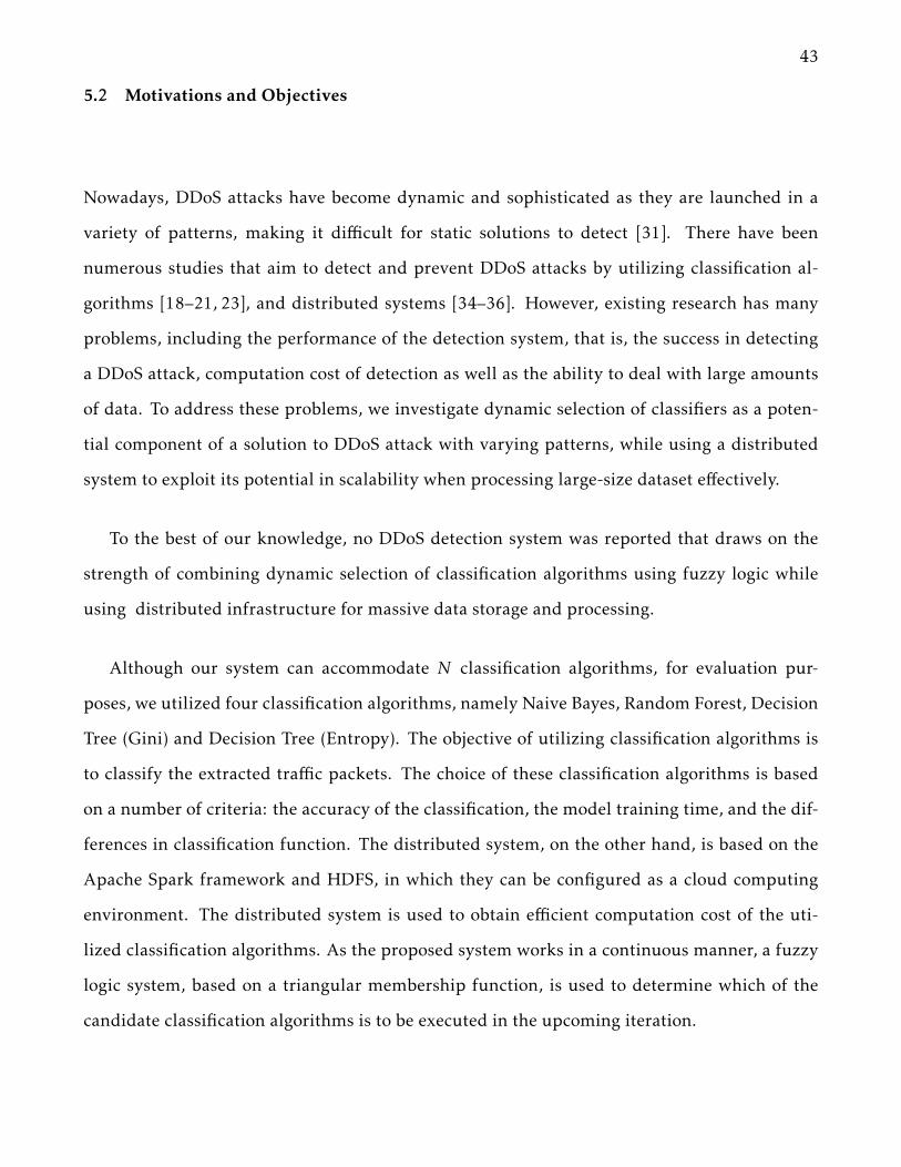
43


Nowadays, DDoS attacks have become dynamic and sophisticated as they are launched in a

variety of patterns, making it difficult for static solutions to detect [31]. There have been

numerous studies that aim to detect and prevent DDoS attacks by utilizing classification al-

gorithms [18–21, 23], and distributed systems [34–36]. However, existing research has many

problems, including the performance of the detection system, that is, the success in detecting

a DDoS attack, computation cost of detection as well as the ability to deal with large amounts

of data. To address these problems, we investigate dynamic selection of classifiers as a poten-

tial component of a solution to DDoS attack with varying patterns, while using a distributed

system to exploit its potential in scalability when processing large-size dataset effectively.

To the best of our knowledge, no DDoS detection system was reported that draws on the

strength of combining dynamic selection of classification algorithms using fuzzy logic while

using distributed infrastructure for massive data storage and processing.

Although our system can accommodate N classification algorithms, for evaluation pur-

poses, we utilized four classification algorithms, namely Naive Bayes, Random Forest, Decision

Tree (Gini) and Decision Tree (Entropy). The objective of utilizing classification algorithms is

to classify the extracted traffic packets. The choice of these classification algorithms is based

on a number of criteria: the accuracy of the classification, the model training time, and the dif-

ferences in classification function. The distributed system, on the other hand, is based on the

Apache Spark framework and HDFS, in which they can be configured as a cloud computing

environment. The distributed system is used to obtain efficient computation cost of the uti-

lized classification algorithms. As the proposed system works in a continuous manner, a fuzzy

logic system, based on a triangular membership function, is used to determine which of the

candidate classification algorithms is to be executed in the upcoming iteration.

44

The research question of this study is whether the proposed system can efficiently de-

tect DDoS attacks by combining the concepts of classification algorithms selection with a dis-

tributed system and a fuzzy logic approach.

We evaluated the performance of classification algorithms and their delays (i.e., model

training time) and validated the fuzzy logic system. The impact of the distributed system on

the training delays is also evaluated using real-world Internet datasets, containing traffic traces,

obtained from CAIDA [42]. The results show that there is a trade-off between the utilized clas-

sification algorithms' accuracies and their delays. We observed that the fuzzy logic system can

effectively select the right classification algorithm based on the traffic status. The distributed

system also has a positive impact on the model training time.

5.3 Chapter Contributions

To the best of our knowledge, there is no DDoS detection system that draws on the strength

of combining N classification algorithms, distributed system techniques, and a selection func-

tion (i.e., fuzzy logic system). By combining these three concepts, this chapter provides the

following contributions:

• DDoS detection system utilizing classification algorithms that are processed in a dis-

tributed system and controlled by a fuzzy logic system.

• A novel procedure for selecting membership functions’ degrees of the proposed fuzzy

logic inputs.

• Experimental evaluation of the classification algorithms’ performances and delays.

• Comparative evaluation of the classification algorithms’ performances and delays for dif-

ferent dataset sizes.

• Experimental evaluation of the fuzzy logic system.

45

Figure 5.1: System workflow

• Experimental evaluation of membership functions’ degrees selection procedure.

5.4 Methodology and System Design

5.4.1 Overview

The proposed DDoS detection system is comprised of three components: classification algo-

rithms, a distributed system, and a fuzzy logic system.

Classification algorithms are used to classify the traffic packets to identify DDoS attacks

out of normal traffic. We leverage a distributed system, i.e., Apache Spark, to accelerate the

execution of these classification algorithms. The fuzzy logic system is employed to deliver a

dynamic selection decision on the classification algorithm to be used for detection.

The employed classification algorithms are Naive Bayes, Decision Tree (Gini), Decision Tree

(Entropy), and Random Forest. Only one of these classification models, as selected by the fuzzy

46

logic system, is used at any given time to classify the traffic.

5.4.2 SystemWorkflow

Figure 5.1 presents an overview of our system workflow and is as follows:

1. A DDoS attack dataset is extracted using the T-shark tool, which is then followed by the

feature extraction that are stored in HDFS.

2. Initially, the classification algorithms are trained to build their models.

3. The classification models are stored and readied to classify incoming data.

4. Fuzzy logic system selects, from the prepared classification models, the one to be used for

classification.

5. The selected model is used to classify the traffic data and stores the results into two

databases:

(a) The training delay and accuracy are stored in a historical database of up to 100 values

for each of the classifier.

(b) Data classified as attack are stored in a DDoS attack dataset.

6. Fuzzy logic system takes classification algorithms’ accuracy, the model training time, and

the traffic volume as inputs and determines which model is to be used on the incoming

data stream.

7. The process is repeated every t time, where t is a parameter to be set.

8. All classification algorithms are re-trained and new models are rebuild if a DDoS is de-

tected and the datasets are updated.

47

5.4.3 Classification Algorithms

Classification algorithms are used to classify the traffic packets to identify DDoS attacks in the

normal traffic. The fuzzy logic is used to determine which of the N classification algorithms

is to be used wherein the classification algorithms are characterized by their accuracy and ex-

ecution delay. Out of the many candidate classification algorithms, we utilize algorithms that

are well known and investigated in terms of their accuracy and delays, namely, Naive Bayes,

Decision Tree (Entropy), Decision Tree (Gini), and Random Forest algorithms. One of the main

reasons to choose these classification algorithms are their differences in the classification pro-

cess and how they affect the accuracy and delays.

Naive Bayes Algorithm

Naive Bayes algorithm is a supervised algorithm that is used widely in many classification

applications [25]. When compared to other algorithms, it provides better accuracy with fewer

features needed as it relies on the concept of independence of attributes [56]. The algorithm is

based in the equation (5.1).

P(h|D) =P(D|h)P(h)

P(D)(5.1)

P(h|D) is the posterior probability of class h target given predictor D attributes. The P(h)

is the prior probability of class. P(D|h) is the probability of predictor given class. P(D) is the

prior probability of predictor.

There are three standard Naive Bayes models: Gaussian, Multinomial, and Bernoulli.

Gaussian is used when features are assumed to have a normal distribution.

Multinomial is used for discrete counts in a text classification problem.

Bernoulli is a binomial model used for an application where the feature vectors are binary (i.e.

0 and 1). As our dataset has only two classes, Attack and Normal, and thus we used Bernoulli

model in our system.

48

Decision Tree (DT)

The DT classification algorithm is a supervised method that builds a model to predict a target

attribute based on the previously trained variable attribute. It has been used in many appli-

cations [57–60]. The prediction accuracy is affected by the number of features in the training

dataset: As the number of features increases, the prediction accuracy increases [56]. The De-

cision Trees are constructed by determining the best split of the set of items in each step. We

used the following two variants of DT.

DT (Entropy) is a measure of the amount of uncertainty in the (data) set S and is given by

equation (5.2).

E =C∑

x=1

−fxlog(fx) (5.2)

where fx is the frequency of label x at a given node and C is the number of unique labels.

DT (Gini impurity) is the measure of the difference in entropy from before to after the set S

is split on an attribute A. It is defined by the equation (5.3).

G =C∑

x=1

fx(1− fx) (5.3)

where fx is the frequency of label x at a given node and C is the number of unique labels.

Random Forest Algorithm (RF)

The Random Forest algorithm [61] is mainly proposed to provide a high accuracy prediction

by combining a large number of decision trees [39]. RF has four main training processes: (1)

re-sampling (bootstrapping), (2) the randomness of feature selection, (3) tree bagging and (4)

full-depth decision tree growing.

49

An RF is an ensemble of N trees T1(X), T2(X), . . ., TN (X), where X= x1, x2, . ., xm is an

m-dimension vector of inputs. The resulting ensemble produces N outputs Y1 = T1(X), Y2 =

T2(X),. . ., YN = TN (X), where Tn(X) is the prediction value by decision tree number n [62].

The final prediction Y ′ of the training will be obtained by applying the majority vote in case

of classification or averaging the prediction results in case of regression as in equation (5.4).

f =1BT

S∑

b=1

fb(x′) (5.4)

where fb is the regression tree and the BT is the tree bagging time.

5.4.4 Fuzzy Logic System

Fuzzy logic was introduced by Zadeh [63] as a technique for describing andmanaging uncertain

information. A fuzzy set specifies a degree of membership, that is a real number between

[0,1], where (1) means entirely true and (0) entirely false. Other numbers in between [1,0] will

represent a degree of truth.

The fuzzy logic system is used to identify the best classification algorithm to be used to

classify the traffic. Simply stated, we use fuzzy logic at each iteration to select the classification

algorithm, from the set of four candidate classification algorithms, to be used to classify the

traffic data. Figure 5.1 shows where the fuzzy logic plays a role in our system.

We propose a fuzzy logic system with three parameters (i.e., inputs): the traffic volume, the

classification algorithm accuracies, and the classification algorithm delays. Figure 5.2 shows

our proposed parameters (i.e., inputs) that are used. Each of the inputs has a set of membership

functions that are represented by a triangular membership function (i.e., Mamdani function).

50

Triangular Membership Function (Mamdani)

Triangular membership function has been applied in many applications because of its simplic-

ity and applicability [64]. Equation (5.5) shows the formal definition of a triangular member-

ship function that is used, which is a group of three points (i.e., three degrees). Equation (5.6)

shows a simple way to calculate a Triangular membership function [65]. We propose a dynamic

technique to set the membership function degrees by using percentile rank. More details are

provided in following section.

Figure 5.2: Inputs of the fuzzy logic system

µH (x) =

⎧⎪⎪⎪⎪⎪⎪⎪⎪⎪⎪⎪⎪⎪⎨⎪⎪⎪⎪⎪⎪⎪⎪⎪⎪⎪⎪⎪⎩

0 x ≤ 0

x − hm− h h ≤ x ≤m

l − xl −m m ≤ x ≤ l

0 l ≤ x

(5.5)

f (x,a,b, c) =Max(Min(x − ab − a ,

c − xc − b ),0) (5.6)

Equation (5.6) shows how the x value is calculated on triangular function, where a, b, and c are

the three degrees of a given membership function.

51

Dynamic Membership Function Degrees

Many fuzzy logic system applications set the membership function degrees’ values statically

[65]. Remember that we propose the fuzzy logic system with three inputs: classification al-

gorithms’ accuracy and delay as well as the current traffic volume. In fact, classification al-

gorithms have different performance rates as well as training time requirements. Therefore,

the membership function degrees for one classification algorithm can not necessarily represent

other classification algorithms. For instance, if a classifier x always has an accuracy higher than

98% and classifier y always has an accuracy less than 80%, then, the membership function

"High" cannot be set from 98% because the classifier y can never be in "High" status.

Therefore, we propose a dynamic technique that sets the membership function degrees for

the accuracy and the delay by using percentile rank. This procedure uses the last hundred

values of the historical results database for both, accuracy and delay. We also introduce two

more membership functions, in addition to those presented in [66], to distinguish between

classification algorithms more accurately. The membership functions for both accuracy and

delay are in the set of {Very High, High, Medium, Low, Very Low}, and their l degrees, of

equation (5.5), are calculated using the percentiles of equation (5.7) in the set of {80, 60, 40,

20, 1}. These values were chosen to represent the five membership functions {Very High, High,

Medium, Low, Very Low} and provide an equal increment distribution by 20%

i =npi100

+0.5 (5.7)

In equation (5.7), n is the total number of observations, which is in our case 100 ∗ 4, where

100 represents the number of runs and 4 is the number of classification algorithms.

For simplicity, we set the membership functions degrees for Traffic volume input statically

as show in Figure 5.3.

52

0 0.2 0.4 0.6 0.8 1 1.2 1.4 1.6 1.8 2

Traffic-Volume 106

0

0.2

0.4

0.6

0.8

1

Deg

ree o

f m

em

bers

hip

Normal High

Figure 5.3: Traffic volume membership function

5.5 Evaluation


The evaluation is conducted in three main steps:

• Analysis of the classification algorithms' performance.

• Analysis of the distributed system.

• Analysis of the fuzzy logic algorithm.

5.5.2 Network Analysis Tool and Software

Dataset

For experimentation purposes we will use two datasets presented in Chapter 3 in Section 3.5:

one with all features that were presented in Table 3.1, called Dataset1, and a second one called

Dataset2, that has the feature presented in Table 3.3.

53

5.5.3 Implementation and Configuration of the Prototype

To examine our proposed system, we set up a testbed consisting of three worker machines and

one master machine. They both run on Ubuntu version 16.04.2 OS with Spark-2.0.2, Hadoop-

2.7.3, and 500 GB of storage. The master machine has a Core i5 CPU and 16 GB of memory. On

the other hand, the worker machines have a Core i7 CPU and 4 GB memory.

5.6 Results

5.6.1 Classification Algorithms Performance Measurements

We evaluated the classification algorithms performance by considering performance measures

that include Accuracy, Precision, Recall, F measure, True Positive rate (TPR), and False Posi-

tive rate (FPR) based on the confusion matrix. Table 3.4 in Section 3.6 already described the

performance measures and the confusion matrix, respectively.

5.6.2 Classification Algorithms Performance Results

In this section, we report the performance rates of the classification algorithms for different

dataset sizes and different number of packets. Tables 5.1, 5.2, 5.3, and 5.4 show the perfor-

mance rates of the classification algorithms for both datasets, Dataset1 and Datset2, for all

different sizes. The Random Forest classifier has the highest accuracy amongst the used clas-

sification algorithms, and it also maintains the lowest false positive when 100,000 packets are

used. The DT(Gini) classifier outperformed other classifiers when we increased the number of

packets to 500,000, 1 million, or 2 million, and was followed very closely in performance by

DT(Entropy). In contrast, The Naive Bayes classifier has the lowest accuracy as we vary the

number of packets.

The DT(Gini) has maintained the highest accuracy as we vary the number of the packets.

However, Random Forest classifier has the lowest false positive rate when the number of pack-

ets is 100,000.

54

Table 5.1: Performance rates for classification algorithms for Dataset1 and Dataset2 for 100K packets

Dataset Classication method Accuracy Recall precision FMeasure F P R T P R

Dataset 1

Naïve Bayes 0.622 0.622 0.625 0.544 0.531 0.622DT(Entropy) 0.970 0.970 0.970 0.970 0.0285 0.970DT(Gini) 0.969 0.969 0.969 0.969 0.0299 0.969Random Forest 0.972 0.972 0.973 0.973 0.0210 0.972

Dataset2


Table 5.2: Performance rates for classification algorithms for Dataset1 and Dataset2 for 500K packets


Dataset 1


Dataset2


Table 5.3: Performance rates for classification algorithms for Dataset1 and Dataset2 for one millionpackets


Dataset 1


Dataset 2


55

Table 5.4: Performance rates for classification algorithms for Dataset1 and Dataset2 for two millionspackets


Dataset 1


Dataset 2

Naïve Bayes 0.60 0.60 0.78 0.66 0.47 0.60DT(Entropy) 0.95 0.95 0.95 0.95 0.19 0.95DT(Gini) 0.95 0.95 0.95 0.95 0.19 0.95Random Forest 0.94 0.94 0.94 0.93 0.32 094

When comparing results between Dataset1 and Dataset2, the Naive Bayes classifier has

an increase in accuracy by 40 % in Dataset2. In contrast, the accuracy slightly decreased in

Dataset2, compared to the same number of packets in Dataset1, for DT(Gini), DT(Entropy),

and Random Forest classifiers.

5.6.3 Analysis of the Distributed System

In this section, the distributed system is evaluated by conducting different scenarios in which

the number of nodes is varied:

1. A baseline in which there is only one machine.

2. A cluster of two machines: one master and one worker node.

3. A cluster of three machines: one master and two worker nodes.

4. A cluster of four machines: one master and three worker nodes.

The classification algorithms’ training times are an important measurement in our system as

we are dealing with DDoS attacks. Remember that we proposed the model training time as

one of the inputs for the fuzzy logic system. Thus, when evaluating the fuzzy system, we only

consider Scenario number (4), in which there are four machines ( one master and three workers

).

56

The dataset sizes and features construction are designed as in Section 3.5. Tables 5.5 and 5.6

show the classifiers training times in milliseconds in all scenarios. The time was calculated by

taking timestamps of the training phase. The best time achieved in each scenario is highlighted.

The overall observations of the results from Tables 5.5, 5.6 and Figures 5.4, 5.5, 5.6, and 5.7 are

as follows:

1. In general, the training time increased as the number of nodes decreased.

2. Naive Bayes is faster than other classifiers in the same scenario with the Dataset2, partic-

ularly when the sizes are 1 million or 2 million. However, it is always faster than other

classifiers in the baseline scenario regardless of the size of the dataset.

3. Random Forest classifier is the slowest in all scenarios. In fact, other classifiers in the

baseline scenario, in which there is no distributed system, are faster than Random Forest

classifier in the scenario in which there are four machines.

4. In comparison between the baseline scenario and the distributed system scenario, the

time in the distributed system decreases by approximately 35% for identical dataset size

with small differences in the percentage across the classification algorithms.

5. In comparison between the distributed system scenarios, the time decreases by approxi-

mately 10% as we increase the number of worker nodes.

57

Table5.5:

Com

parisonde

lays

forclassification

algo

rithmsfordiffe

rent

sizesof

Dataset1an

dDataset2in

millisecon

din

diffe

rent

numbe

rof

node

s

Num

berof

node

sDataset

name

Classification

metho

dsDataset

size

100,00

050

0,00

01Million

2Millions

Baseline

(Nodistribu

tedsystem

)

Dataset1

Naïve

Bayes

1187

013

197

2423

228

936

DT(G

ini)

1668

424

346

6594

012

9413

DT(Entropy

)14

211

2400

153

920

1293

00

Ran

dom

Forest

5099

618

0408

3224

7757

7800

Dataset2

Naïve

Bayes

1694

119

882

1553

932

121

DTGini

2048

623

750

3045

976

277

DT(Entropy

)17

693

2135

227

356

6630

7

Ran

dom

Forest

7391

016

9692

3283

2675

3957

Master

+

oneworke

rmachine

Dataset1

Naïve

Bayes

8231

9399

1914

818

465

DT(G

ini)

7429

9733

3944

766

278

DT(Entropy

)64

7896

0837

549

6431

7

Ran

dom

Forest

2408

969

965

1584

8926

8745

Dataset2

Naïve

Bayes

8853

1053

289

4019

958

DTGini

7202

8896

1103

243

413

DT(Entropy

)65

4485

9210

233

4294

6

Ran

dom

Forest

2651

958

314

1015

4823

4622

58

Table5.6:

Com

parisonde

lays

forclassification

algo

rithmsfordiffe

rent

sizesof

Dataset1an

dDataset2in

millisecon

din

diffe

rent

numbe

rof

node

s

Num

berof

node

sDataset

name

Classification

metho

dsDataset

size

100,00

050

0,00

01Million

2Millions

Master

+

twoworke

rmachine

s

Dataset1

Naïve

Bayes

9629

8171

8296

1494

7

DT(G

ini)

7292

9316

1190

925

493

DT(Entropy

)73

4693

5511

606

2824

4

Ran

dom

Forest

2372

765

725

1120

0420

6908

Dataset2

Naïve

Bayes

1072

686

0891

0694

59

DTGini

6944

9048

1046

014

490

DT(Entropy

)64

4482

5810

051

1488

0

Ran

dom

Forest

2446

854

569

9145

220

0155

Master

+

threeworke

rmachine

s

Dataset1

Naïve

Bayes

1040

410

157

1052

715

328

DT(G

ini)

8245

1146

814

758

2418

9

DT(Entropy

)75

6510

080

1297

131

708

Ran

dom

Forest

2371

168

386

1188

5120

6809

Dataset2

Naïve

Bayes

9805

9554

8547

8225

DT(G

ini)

7092

8948

1051

015

187

DT(Entropy

)66

2289

5110

349

1380

4

Ran

dom

Forest

2479

858

067

9593

718

8790

59

�

�

��

��

��

��

��

��

��

��

� ��

��

��

Figure 5.4: Delay of Naive Bayes classifier in different distributed system scenarios

The percentages in observations (4) and (5) are calculated by the equation 5.8.

|δV1|σV22

×100 (5.8)

where V1 is the delay in one scenario and V2 is the delay in another scenario. From the ob-

servation above, there is a notable indication that the distributed system has a positive impact

on the classification algorithms’ training time. The number of nodes in the Spark cluster is

inversely proportional to the classification algorithms training time. We can conclude that the

more cluster nodes, the faster the DDoS attack detection system.

Figure 5.8 shows a comparison view of the processing delays for all examined classification

algorithms for scenario (4).

60

�

��

��

��

��

��

��

��

��

��

��

��

��

Figure 5.5: Delay of DT-Gini classifier in different distributed system scenarios

�

��

��

��

�

��

��

��

��

��

��

��

��

Figure 5.6: Delay of DT-Entropy classifier in different distributed system scenarios

61

�

��

��

��

��

��

��

��

!��

��

��

� ��

��

��

Figure 5.7: Delay of Random Forest classifier in different distributed system scenarios

Figure 5.8: Classification algorithms delays and size

62

0.9 0.91 0.92 0.93 0.94 0.95 0.96 0.97 0.98 0.99 1

Accuracy

0

0.2

0.4

0.6

0.8

1

Degre

e o

f m

em

bers

hip

Accuracy memebership function for the large dataset with 100 thuosand packets size

Very High

High

Mediam

Low

Very Low

0.9 0.91 0.92 0.93 0.94 0.95 0.96 0.97 0.98 0.99 1

Accuracy

0

0.2

0.4

0.6

0.8

1

Degre

e o

f m

em

bers

hip

Accuracy memebership function for the large dataset with 500 thousand packets size

Very High

High

Mediam

Low

Very Low

0.9 0.91 0.92 0.93 0.94 0.95 0.96 0.97 0.98 0.99 1

Accuracy

0

0.2

0.4

0.6

0.8

1

Degre

e o

f m

em

bers

hip

Accuracy memebership function for the large dataset with 1 million packets size

Very High

High

Mediam

Low

Very Low

0.9 0.91 0.92 0.93 0.94 0.95 0.96 0.97 0.98 0.99 1

Accuracy

0

0.2

0.4

0.6

0.8

1

Degre

e o

f m

em

bers

hip

Accuracy memebership function for the large dataset with 2 millions packet size

Very High

High

Mediam

Low

Very Low

Figure 5.9: Accuracy membership function for Dataset1

5.6.4 Analysis of Fuzzy Logic System

Remember that fuzzy logic is used in our system to select the next classifier in a given time

interval. Tables 5.7 and 5.8 show the setup rules between inputs. We divided the rules into

two main categories based on the traffic volume (i.e. High or Medium). In each category, there

are twenty-five chances of being used to precisely distinguish between different classification

algorithms. When the number one (1) appears in the table column "Chance", then the chance

is high, whereas twenty five (25) indicates a low chance.

Figures 5.9 and 5.10 show the dynamic degrees of membership functions of the accuracy

input, for Dataset1 and Dataset2, respectively. The membership functions’ degrees are similar

to each other with approximately 1% differences between different dataset sizes for Dataset1.

However, for the Dataset2, the similarity is decreased even more than 1%. Therefore, it is an

evidence in support that our proposed membership functions were correctly managed.

Figures 5.11 and 5.12 show the dynamic degrees for membership functions of the delay, for

63

Table 5.7: Rules of members in which the traffic volume is High

Traffic Accuracy Delay Chance

High Very Low Very Low 1

High Low Very Low 2

High Medium Very Low 3

High High Very Low 4

High Very High Very Low 5

High Very Low Low 6

High Low Low 7

High Medium Low 8

High High Low 9

High Very High Low 10

High Very Low Medium 11

High Low Medium 12

High Medium Medium 13

High High Medium 14

High Very High Medium 15

High Very Low High 16

High Low High 17

High Medium High 18

High High High 19

High Very High High 20

High Very Low Very High 21

High Low Very High 22

High Medium Very High 23

High High Very High 24

High Very High Very High 25

64

Table 5.8: Rules of members in which the traffic volume is Medium

Traffic Accuracy Delay Chance

Medium Very High Very Low 1

Medium Very High Low 2

Medium Very High Medium 3

Medium Very High High 4

Medium Very High Very High 5

Medium High Very Low 6

Medium High Low 7

Medium High Medium 8

Medium High High 9

Medium High Very High 10

Medium Medium Very Low 10

Medium Medium Low 12

Medium Medium Medium 13

Medium Medium High 14

Medium Medium Very High 15

Medium Low Very Low 16

Medium Low Low 17

Medium Low Medium 18

Medium Low High 19

Medium Low Very High 20

Medium Very Low Very Low 21

Medium Very Low Low 22

Medium Very Low Medium 23

Medium Very Low High 24

Medium Very Low Very High 25

65

0.9 0.91 0.92 0.93 0.94 0.95 0.96 0.97 0.98 0.99 1

Accuracy

0

0.2

0.4

0.6

0.8

1

Degre

e o

f m

em

bers

hip

Accuracy memebership function for the small dataset with 100 thuosand packets size

Very High

High

Mediam

Low

Very Low

0.9 0.91 0.92 0.93 0.94 0.95 0.96 0.97 0.98 0.99 1

Accuracy

0

0.2

0.4

0.6

0.8

1

Degre

e o

f m

em

bers

hip

Accuracy memebership function for the small dataset with 500 thousand packets size

Very High

High

Mediam

Low

Very Low

0.9 0.91 0.92 0.93 0.94 0.95 0.96 0.97 0.98 0.99 1

Accuracy

0

0.2

0.4

0.6

0.8

1

Degre

e o

f m

em

bers

hip

Accuracy memebership function for the small dataset with 1 million packets size

Very High

High

Mediam

Low

Very Low

0.9 0.91 0.92 0.93 0.94 0.95 0.96 0.97 0.98 0.99 1

Accuracy

0

0.2

0.4

0.6

0.8

1

Degre

e o

f m

em

bers

hip

Accuracy memebership function for the small dataset with 2 millions packet size

Very High

High

Mediam

Low

Very Low

Figure 5.10: Accuracy membership function for Dataset2

Dataset1 and Dataset2, respectively.

Figure 5.13 shows the chance level of classifier selection for Dataset1 for the packet size

of 100,000, 500,000, 1 million, and 2 million. Note that we set the threshold of traffic at the

value of 100 in which the traffic status is changed from a Normal to High volume traffic status.

Recall that the chances’ indexes of the fuzzy logic system are set in an ascending order so

that the higher the index number, the lower the chance. Thus, DT (Gini) classifier has more

chance to be selected as the best candidate when the traffic volume is in the Normal status. In

contrast, Naive Bayes has mostly higher chances when the traffic volume is in the "High" status.

Figure 5.14 shows the chance level of classifier selection for Dataset2 for 100,000 , 500,000 ,

1 million, and 2 million number of packets. The DT (Gini) classifier has higher chances, in

all different sizes, wherein traffic volume is in the Normal status. The same trend goes for

Naive Bayes classifier when the Traffic volume has High status. However, Naive Bayes loses the

chance when the number of packets is 2 million. Remember that some of the DDoS attacks

66

0 0.1 0.2 0.3 0.4 0.5 0.6 0.7 0.8 0.9 1

Delay

0

0.2

0.4

0.6

0.8

1

Degre

e o

f m

em

bers

hip

Delay memebership function for the large dataset with 100 thuosand packets size

Very Low

Low

Mediam

High

Very High

0 0.1 0.2 0.3 0.4 0.5 0.6 0.7 0.8 0.9 1

Delay

0

0.2

0.4

0.6

0.8

1

Degre

e o

f m

em

bers

hip

Delay memebership function for the large dataset with 500 thousand packets size

Very Low

Low

Mediam

High

Very High

0 0.1 0.2 0.3 0.4 0.5 0.6 0.7 0.8 0.9 1

Delay

0

0.2

0.4

0.6

0.8

1

Degre

e o

f m

em

bers

hip

Delay memebership function for the large dataset with 1 million packets size

Very Low

Low

Mediam

High

Very High

0 0.1 0.2 0.3 0.4 0.5 0.6 0.7 0.8 0.9 1

Delay

0

0.2

0.4

0.6

0.8

1

Degre

e o

f m

em

bers

hip

Delay memebership function for the large dataset with 2 millions packet size

Very Low

Low

Mediam

High

Very High

Figure 5.11: Delay membership function for Dataset1

0.9 0.91 0.92 0.93 0.94 0.95 0.96 0.97 0.98 0.99 1

Accuracy

0

0.2

0.4

0.6

0.8

1

Degre

e o

f m

em

bers

hip

Accuracy memebership function for the small dataset with 100 thuosand packets size

Very Low

Low

Mediam

High

Very High

0.9 0.91 0.92 0.93 0.94 0.95 0.96 0.97 0.98 0.99 1

Accuracy

0

0.2

0.4

0.6

0.8

1

Degre

e o

f m

em

bers

hip

Accuracy memebership function for the small dataset with 500 thousand packets size

Very Low

Low

Mediam

High

Very High

0 0.1 0.2 0.3 0.4 0.5 0.6 0.7 0.8 0.9 1

Delay

0

0.2

0.4

0.6

0.8

1

Degre

e o

f m

em

bers

hip

Delay memebership function for the small dataset with 1 million packets size

Very Low

Low

Mediam

High

Very High

0 0.1 0.2 0.3 0.4 0.5 0.6 0.7 0.8 0.9 1

Delay

0

0.2

0.4

0.6

0.8

1

Degre

e o

f m

em

bers

hip

Delay memebership function for the small dataset with 2 millions packet size

Very Low

Low

Mediam

High

Very High

Figure 5.12: Delay membership function for Dataset2

67

Selected algorithm chance level for the large

dataset with 100 thousand packets size

0 50 100 150 200

Traffic volume

0

50

100

150

200

250

300

Ch

an

ce

le

ve

l

DT (Entropy)

DT (Gini)

Random Forest

Naive Bayes

Traffic Volume



0 50 100 150 200

Traffic volume

0

50

100

150

200

250

Ch

an

ce

le

ve

l

DT (Entropy)

DT (Gini)

Random Forest

Naive Bayes

Traffic Volume


dataset with 1 million packets size

0 50 100 150 200

Traffic volume

0

50

100

150

200

250

Ch

an

ce

le

ve

l

DT (Entropy)

DT (Gini)

Random Forest

Naive Bayes

Traffic Volume



0 50 100 150 200

Traffic volume

0

50

100

150

200

250

300

Ch

an

ce

le

ve

l

DT (Entropy)

DT (Gini)

Random Forest

Naive Bayes

Traffic Volume

Figure 5.13: Selected algorithm chance level for the Dataset1

Selected algorithm chance level for the small


0 50 100 150 200

Traffic volume

0

50

100

150

200

250

300

Ch

an

ce level

DT (Entropy)

DT (Gini)

Random Forest

Naive Bayes

Traffic Volume



0 50 100 150 200

Traffic volume

0

50

100

150

200

250

Ch

an

ce level

DT (Entropy)

DT (Gini)

Random Forest

Naive Bayes

Traffic Volume



0 50 100 150 200

Traffic volume

0

50

100

150

200

250

Ch

an

ce level

DT (Entropy)

DT (Gini)

Random Forest

Naive Bayes

Traffic Volume



0 50 100 150 200

Traffic volume

0

50

100

150

200

250

300C

han

ce level

DT (Entropy)

DT (Gini)

Random Forest

Naive Bayes

Traffic Volume

Figure 5.14: Selected algorithm chance level for the Dataset2

68

20

21

40

Traffic-Volume

10 6

60

1

Ch

an

ce

Accuracy

100 thousand total packets number

0.95

80

0 0.9

20

21

40

Traffic-Volume

10 6

60

1

Ch

an

ce

Accuracy


0.95

80

0 0.9

20

21

40

10 6

Traffic-Volume

60

1

Ch

an

ce

Accuracy

One million total packets number

0.95

80

0 0.9

2

20

1

40

10 6

Traffic-Volume

1

Ch

an

ce

Accuracy

Two million total packets number

0.95

60

80

0 0.9

Figure 5.15: Surface view illustrates the relationship between traffic and accuracy for Dataset1 forpacket size of 100 thousands, 500 thousands, 1 millions, and 2 millions

20

21

40

10 6

Traffic-Volume

60

1

Ch

an

ce

Accuracy


0.95

80

0 0.9

20

21

40

10 6

Traffic-Volume

60

1

Ch

an

ce

Accuracy


0.95

80

0 0.9

20

21

40

10 6

Traffic-Volume

60

1

Ch

an

ce

Accuracy


0.95

80

0 0.9

20

21

40

10 6

Traffic-Volume

60

1

Ch

an

ce

Accuracy


0.95

80

0 0.9

Figure 5.16: Surface view illustrates the relationship between traffic and accuracy for Dataset2 for apacket size of 100 thousands, 500 thousands, 1 millions, and 2 millions

are launched to exhaust the victim with a low traffic volume over a period of time. Therefore,

Naive Bayes classifier would not be selected in such a situation where the high volume traffic is

not the main characteristic of the DDoS attack.

Figures 5.15 and 5.16 show a surface view of the relationship between the traffic volume

and the classification accuracy for Dataset1 and Dataset2, respectively, in a packet size of 100

thousand, 500 thousand, 1 million, and 2 million. The traffic volume is directly proportional

to the classification algorithm accuracy. The selection function (i.e., fuzzy logic system) will

select a classifier that has more accurate classification than the classifier with less accurate

classification.

20

21

40

Traffic-Volume

10 6 1

Ch

an

ce

Delay

60


0.5

80

0 0

2

20

1

40

Traffic-Volume

10 6 1

Ch

an

ce

Delay


0.5

60

80

0 0

20

21

40

Traffic-Volume

10 6 1

Ch

an

ce

Delay

60


0.5

80

0 0

2

20

1

40

Traffic-Volume

10 6 1

Ch

an

ce

Delay


0.5

60

80

0 0

Figure 5.17: Surface view illustrates the relationship between traffic and delay for Dataset1 for a packetsize of 100 thousand, 500 thousand, 1 million, and 2 millions

69

2

20

1

40

10 6

Traffic-Volume

1

Ch

an

ce

Delay


60

0.5

80

0 0

2

50

1

60

70

Traffic-Volume

10 6 1

Ch

an

ce

Delay


0.5

80

90

0 0

2

40

1

Traffic-Volume

10 6 1

Ch

an

ce 60

Delay


0.5

80

0 0

2

20

1

40

Traffic-Volume

10 6 1

Ch

an

ce

Delay


0.5

60

80

0 0

Figure 5.18: Surface view illustrates the relationship between traffic and delay for Dataset2 for the sizesof 100 thousand, 500 thousand, 1 million, and 2 million packets

Figures 5.17 and 5.18 show the relationship between the traffic volume and the classifica-

tion algorithms delay of Dataset1 and Dataset2, respectively, in packet sizes of 100 thousand,

500 thousand, 1 million, and 2 million. The traffic volume is directly proportional to the classi-

fication algorithm delay. When the traffic volume is high, the selection function algorithm with

a low delay.

5.7 Discussion

In this section, we discuss the benefits, limitations, and possible future work for our system.

In the DDoS detection system using classification algorithms, the objective is to classify the

network traffic data. To the best of our knowledge, most of the existing solutions rely on one

classifier. These solutions are not reliable since the DDoS attack patterns have become more

dynamic and challenging to detect [31]. Moreover, most DDoS attacks have a massive amount

of data that needs more consideration while developing the DDoS detection system. For these

reasons, we propose a DDoS detection system that leverages a number of classification algo-

rithms and a distributed system. Furthermore, our system effectively uses the fuzzy logic to

select at-run-time an appropriate classifier, from a set of candidate classifiers, to be used for

classification of incoming data for a period of time after which another classifier may be se-

lected.

70

5.7.1 Classification Algorithms

In general, Big Data researchers have been debating whether to usemore features from a dataset

or to use the best selection of features. Some studies recommend using a dataset with more

features to accommodate the selection feature algorithm with better classification algorithms

performance as well as alternatives to find the best subset of features [67]. However, other

researchers claim that fewer features result in improvements in simplicity and in the classifi-

cation algorithms performance as well as delays [68–70].

Remember that the DT (Gini) and the DT (Entropy) were the best candidate regarding ac-

curacy. However, the Naive Bayes algorithm has the lowest delay, which makes it the best

candidate algorithm when processing delay is most important. In contrast, the Random Forest

algorithm has the highest delays, but it had the best accuracy for Dataset1 when the number

of packets was 100,000. Remember that in our experiments the overfitting problem is being

addressed by increasing the dataset size and the randomization technique for training and test-

ing.

5.7.2 Distributed System

The faster the model training time, more data can be processed, and more data processed, bet-

ter the accuracy [29]. In this research, the lower model training times achieved through Spark

showed its advantages of faster training time of the classification algorithms. The results also

show the differences in the training times between Dataset1 and Dataset2 in different experi-

mental scenarios. We found that the transition points between Scenario 1 (i.e., non distributed

environment), and other scenarios, (i.e., distributed environment), are dramatic as the training

times decreased when using a distributed system. Therefore, in general, using classification

algorithm within the distributed system allows two main benefits: more data to be processed

resulting in a high model accuracy as shown in Tables 5.1, 5.2, 5.3, and 5.4, and faster model

training times as shown in the Tables 5.5 and 5.6.

71

5.7.3 Fuzzy Logic System

It is worth noticing that, with various classification algorithms, there exists a trade-off between

accuracy and training delay. It is essential for the DDoS detection system to use a classifier with

high performance and fast training delay [68]. In our system, we consider both the accuracy and

the delay of classification algorithms by employing the fuzzy logic system. The results show

that using the fuzzy logic system provides a reliable solution to select the right algorithm at the

right traffic volume. The concept of fuzzy logic makes our system dynamic in the application

of classification algorithms. Unlike the study done by Song and Liu [18], where they propose a

combination of detection system (i.e., a K-NN algorithm) and a distributed system (i.e., Storm),

our system is dynamic and has a number of classification algorithms that are ready to be used

seeking the trade-off of accuracy and delay.


We propose a DDoS detection system composed of three components: a set of classification

algorithms, a distributed system, and a fuzzy logic system. We evaluate our system through

experimentation. Firstly, the performance of the classification algorithms is evaluated. Sec-

ondly, the impact of the distributed system is analyzed using different configuration scenarios,

different data set sizes and number of classifiers. Thirdly, the validation and the effectiveness

of the fuzzy logic system is examined.

The results of the classification algorithms' performance show that there is a trade-off be-

tween the accuracy and the delay. In general, classification algorithms have higher performance

rates and delays when using Dataset1. In contrast, classification algorithms have lower perfor-

mance rates and delays when using Dataset2. However, that is not always the case as the model

training times are inversely proportional to the number of the nodes in the Spark cluster. The

fuzzy logic system, on the other hand, can effectively select the right classification algorithm

from a set of candidate classifier.

72

5.9 Limitations and Future Work

In the future we will be focusing on the following points:

1. Currently, our system is designed to analyze static network traffic data. Our system is

able of capturing and storing network traffic data in an HDFS database, waiting for batch

processing. We will extend the proposed method to handle real streaming data from all

sources with the objective to detect DDoS attack in near real-time.

2. The iteration T time was statically set. However, in the future, we will investigate an

effective and dynamic mechanism to update the iteration time.

3. The dataset was updated each iteration when the traffic data is classified as a DDoS attack.

However, currently, our system uses the same dataset with different sizes and different

feature dimensions to simulate the update process. In the future, we will investigate the

update process including data labelling as well as the increase of the dataset size.

Chapter 6

Features Selection Framework Based on Chi-Square Algorithm

6.1 Overview

Features selection algorithms provide a process for removing a subset of features, which are not

significant to the applied classification, from a dataset. Applying algorithms to select features

hasmany potential benefits, and it has been used inmany applications [3,4,71]. First, themodel

training is faster as it removes useless attributes from the original dataset. Secondly, it also

reduces the matrix size of a model and thus makes it easier to interpret. Moreover, it reduces

the overfitting of the model [4]. Due to aforementioned benefits, we propose a framework to

improve the accuracy of the DDoS detection system by feature selection algorithm with the

objective that it chooses the best feature selection algorithm, from a set of prepared algorithms.


6.2.1 Motivation

FS and classification play crucial role in identifying attack packets. Research has shown that

using FS to reduce noise and remove redundant data positively impacts the overall accuracy

and speeds up the overall of building of the machine learning algorithm model by reducing

the dataset dimensions [72–75]. In short, FS eliminates inappropriate and redundant instances

from the dataset, thereby improving the overall performance.

73

74

6.2.2 Objective

The objective of this Chapter is to investigate the impact of FS on the performance of the classi-

fication algorithms. Among the various FS algorithms, the Chi-Square algorithm is considered

a simple but efficient and successful feature eliminator. Understanding the impacts of using

the Chi-Square variants on the performance of the four classifiers, namely NB, DT based on

Entropy, Logistic Regression (LR) and RF, is crucial to determine the best combination of FS

and classification methods for accurately predicting a DDoS attack.

The fundamental research questions this Chapter addresses are:

1. Do Chi-Square variants used in FS impact the performance of the classification algorithm

when used to predict a DDoS attack?

2. Do the Chi-Square variants decrease the classifiers’ training times and notably improve

the accuracy of the prediction?


6.3.1 Background

DDoS Attack

In DDoS attacks, the attackers flood the victim’s server with a large volume of packets, which

consumes computational and network resources rendering them unavailable for processing

packets of legitimate users. In most cases, the victims have no prior knowledge that they

are being attacked until it is too late, in which case the victims have no choice but to shut

down their services to prevent any damage. A DDoS attack involves an explicit attempt to stop

the legitimate users from accessing service [76]. Classification of DDoS attacks into Volume-

based attacks, Protocol attacks, and Application layer attacks has already been discussed in

Section 2.4

75

6.3.2 Literature Review

Several studies have investigated FS algorithms while developing a DDoS attack detection sys-

tem [17,77–85].

Balkanli et al. [77] investigated well-known FS algorithms, namely Chi-Square and Sym-

metrical Uncertainty, together with the DT classifier for Backscatter DDoS detection system.

They evaluated the performance of their proposed detection system on different traffic traces

provided by CAIDA. Their results show that the C4.5 Decision Tree classifier with only seven

features could achieve more than 95% precision in detecting new Backscatter DDoS attack pat-

terns.

Barati et al. [78] proposed a feature selection approach as a wrapper feature selection for

DDoS detection using a Genetic Algorithm (GA). They employed an Artificial Neural Network

(ANN) as a classifier and considered accuracy as a fitness function for a wrapper feature selec-

tion. They claimed that their proposed approach resulted in very promising findings compared

to earlier studies.

Doshi et al. [80] proposed and analyzed DoS detection for IoT devices. They chose a selected

feature set, which was mainly based on the hypothesis that differences exist between network

IoT and non-IoT traffic patterns. They evaluated their hypothesis by using five classifiers: K-

Nearest Neighbours (KNN), RF, DT, Support Vector Machine (SVM), and DNN. They reported

that the five employed classifiers showed accuracy higher than 99%. However, it would be

interesting to compare the results with different sets of features.

Feng et al. [81] proposed a feature selection procedure for early DDoS attack detection.

Their objective was to find if all features were essential to detect DDoS attacks at an early stage.

They utilized SVM and PCA for feature selection. They also adapted RF as a classifier. Their

results show that applying more features performed better most of the time.

Yusof et al. [82] proposed a DDoS adaptive detection system using Characteristic-Based Fea-

tures (CBF) and a Consistency-based Subset Evaluation (CSE) to select the significant features

76

in the well-known NSL-KDD dataset. A simple majority vote is used to merge the combination

of two outputs from the feature selection methods. They perform a majority vote upon selected

features with a predefined threshold. They evaluated their feature selection using the Extreme

Learning Machine (ELM) classifier. They claimed that their system improved performance as

well as testing time.

Harbola et al. [83] analysed selected feature selection algorithms using a DDoS attack dataset

from the well-known NSL-KDD CUP 99. Their objective was to improve DDoS detection by

applying three feature selection methods: an Attribute Score, Attribute Rank, and Attribute

Subset using Greedy Forward Selection (GFS). The KNN algorithm was utilized later to classify

the packets.

Htun PT et al. [85] implemented a combination of RF and KNN algorithms for features se-

lection to support DoS detection attacks. Wang et al. [84] argued that incorrect FS may remove

significant features and thus lower the accuracy of an attack prediction. They proposed a fea-

ture selection method based on the combination of RF and SVM in which the RF performs the

feature selection and SVM rescreens the selected features to ensure that there are no falsely

eliminated critical features.

To the best of our knowledge, no author has combined the power of Apache Spark and

Hadoop cluster and the effectiveness of Chi-Square to select features for subsequent detection

of DDoS attack which is the approach we are investigating herein:

• This study is unique in that it draws on the strength of analyzing Chi-Square variants

when combined with the distributed computing environment (i.e., Apache Spark and

Apache Hadoop).

• Evaluation of this approach indicates promising experimental results in accuracy as well

as in delays.

77

� ��

��

��

��

��

��

��

��

��

��

� ��

��

��

��

��

��

�

�

�

�

�

�

Figure 6.1: Framework components and workflow

6.4 System Architecture

6.4.1 Overview

This Chapter focuses on the FS in which the dataset is pre-processed using six Chi-Square vari-

ants and then re-structured with features derived by the FS methods. The structured dataset is

stored in the HDFS to be used by the classification algorithms. Fig. 6.1 shows the components

and workflow in our system.

6.4.2 Chi-Square feature selection approaches

The Chi-Square is one of the most robust feature selection approaches that has been widely

used. Many researchers have utilized the Chi-Square algorithm for DDoS attacks [77,78,80,81,

78

Table 6.1: Chi-Square test table to calculate the χ2 score of a feature X

ClassifiedPositive

ClassifiedNegative Total

Feature Xoccurs CP CN CP + CN =

FMFeature Xnot occurs NCP NCN NCP + NCN =

Y - FM

Total CP + NCP = Z CN + NCN = Z -Y Y

83]. A major advantage of the Chi-Square algorithm is that it is designed to analyze categorical

data.

FS attempts to identify important features for use in the model construction. It reduces

the size of the feature space, which can improve both the speed and the model learning per-

formance. It operates on labelled data with categorical features. Chi-Square test uses inde-

pendence to decide which features to choose. Equation 6.1 shows how Chi-Square is calcu-

lated [86,87].

χ2 =n∑

k=1

(Ok −Ek)2

Ek(6.1)

where O is the exact observed value for each class and E is the expected number based on

the distribution of the samples for the corresponding category [88]. Table 6.1 shows how the

observed and expected values are obtained. CP and CN denote the respective observed positive

and negative values that include feature X. NCP and NCN denote the number of positive and

negative samples that do not include feature X, respectively. Therefore, the expected values

ECP , ECN , ENCP , and ENCN can be calculated in a manner similar to equation (6.2) that shows

the definition of ECP .

ECP = (CP +NCP)CP +CN

Y(6.2)

The equation is used for six selection methods , variants of Chi-square: Best Top Features,

Percentile, False positive rate (Fpr), False discovery rate (Fdr), Family-wise error rate (Fwe), and

Generic.

79

Best-Top-Features (Chi-Best-K) The method keeps a fixed quantity of top features according

to a Chi-squared test. It is similar to yielding the features of the most predictive power. Thus,

this method will always choose the top ten features based on the Chi-Square [89].

Percentile (Chi-Percentile) This is similar to Chi-Best-K, but it chooses a fraction of total

features rather than a fixed number. For this method, we choose the percentile to be 20 % as

per [89].

Fpr (Chi-Fpr) This accepts every feature whose p-values are under a threshold, thus manag-

ing the false positive rate of the selection. For our implementation, we set the threshold false

positive rate to be 0.01 [89].

Fdr (Chi-Fdr) This uses the Benjamini-Hochberg procedure to choose total features whose

false discovery rate is below a threshold. Here, we set the threshold of the false discovery rate

α parameter to be 0.01 [89].

Fwe (Chi-Fwe) The method chooses all features whose p-values are below a threshold. The

threshold is scaled by 1 divided by the number of features and thus controlling the family-wise

error rate of selection. The family-wise error rate threshold is set to be 0.01 [89].

Generic (Chi-Generic) This allows the performing of univariate feature selection with a con-

figurable strategy [89].

80

6.5 Evaluation


Cluster Setting

A testbed consisting of an Apache Spark cluster that has a master machine and three worker

nodemachines was set up to examine the proposed system. Themaster and the workers operate

on a Linux Ubuntu system with 500 GB HDD. The master machine has a Core i5 CPU and 16

BG of RAM, while the worker nodes have a Core i7 CPU and 4 GB RAM. The cluster runs

Apache Spark-2.2.1 integrated with Hadoop.

Dataset

The original dataset containing real-world internet traffic was acquired from CAIDA [42], from

which further binary dataset was generated in LIBSVM data format in the form of {xi , yi},

where i = 1.....n, in which x is a multi-dimensional input vector, and y {0,1} represents the

predicted result (0: regular traffic and 1: attack). The features were extracted for UDP and

TCP packets, respectively, using T-shark. The original dataset was duplicated and constructed

into four different samples’ sizes; 100,000 (100 K), 500,000 (500 K), one million (1 M), and two

million (2 M) packets.


There were two separate experiments performed on FS and the classifiers. The FS experiments

were run 20 times, and we report averages. The FS methods were performed on four datasets

resulting in 24 new datasets being produced. The datasets were stored in HDFS to be processed

by the classification algorithms. The performance of the classification algorithms was evaluated

by calculating the prediction accuracy. The accuracy is calculated, as shown in the equation 3.1,

using the confusion matrix shown in Table 3.4 being presented in Chapter 3. The classification

algorithms randomly use 70% of dataset samples for training and 30% for testing. We used the

81

average of the models’ training times, which is reported in milliseconds, and the average of the

prediction accuracy.

The evaluation was conducted in three main steps:

• Analysis of the FS algorithms’ performance.

• Analysis of the classifiers’ performance and the impact of utilizing FS.

• Analysis of the classifiers’ training time and the FS methods’ processing delays.

6.5.3 Analysis of the Feature Selection Algorithms’ Performance

Table 6.2 shows the features that are forming the original dataset. The dataset has 49 features

that include information such as the IP address, the packet type, frames’ info., port numbers,

and some flags.

Table 6.2: Extracted feature from the original packets

[1]: ip.src [2]: ip.dst [3]: tcp.srcport [4] : udp.srcport[5]: tcp.dstport [6] : udp.dstport [7]: ip.proto [8] : ssl.handshake.ciphersuite[9]: ssl.handshake.version [10]: _ws.col.info [11]: frame.number [12]: frame.time_delta[13]: frame.len [14]: frame.cap_len [15]: frame.marked [16]: ip.len[17]: ip.flags [18]: ip.flags.rb [19]: ip.flags.df [20]: ip.flags.mf[21]: ip.ttl [22]: ip.frag.offset [23]: ip.checksum [24]: tcp.len[25]: tcp.seq [26]: tcp.nxtseq [27]: tcp.ack [28]: tcp.hdr_len[29]: tcp.flags [30]: tcp.flags.cwr [31]: tcp.flags.fin [32]: tcp.flags.urg[33]: tcp.flags.ack [34]: tcp.flags.push [35]: tcp.flags.reset [36]: tcp.flags.syn[37]: tcp.flags.ecn [38]: tcp.window_size [39]: tcp.checksum_bad [40]: udp.length[41]: udp.checksum_coverage [42]: udp.checksum [43]: smb.cmd [44]: tcp.checksum[45]: tcp.checksum_good [46] : udp.checksum_good [47]: udp.checksum_bad [48]: ip.checksum_good[49]: ip.checksum_bad

Tables 6.3, 6.4, 6.5, and 6.6 show the features selected by different FS algorithms from the

original dataset of size 100 K, 500 K, 1 M and 2 M, respectively. Note that the selected features

are listed by their index numbers from Table 6.2. Although the FS algorithms selected different

feature sets, some features were selected by many FS methods: the set {1, 2, 3, 4, 6, 26, 27, 28,

39, 43} includes indices of features that were chosen by most of the FS algorithms.

82

Table 6.3: Selected features, for the dataset size 100K, based on Chi-Square variants presented by theirindex from table 6.2

Algorithm Selected featuresChi-Best-K 1,2,3,4,6,26,27,28,39,43

Chi-Fdr 1,2,3,4,5,6,7,14,15,17,18,20,21,22,23,24,25,26,27,28,29,30,34,37,39,40,41,43

Chi-Fpr 1,2,3,4,5,6,7,14,15,17,18,20,21,22,23,24,25,26,27,28,29,30,34,37,39,40,41,43

Chi-Fwe 1,2,3,4,5,6,7,14,15,17,18,21,22,23,24,25,26,27,28,29,30,3437,39,40,41,43

Chi-Generic 1,2,3,4,6,26,27,28,39,43Chi-Percentile 1,2,3,4,5,6,26,27,28,39,43

Table 6.4: Selected features, for the dataset size 500K, based on Chi-Square variants presented by theirindex from table 6.2


Chi-Fdr 1,2,3,4,5,6,13,14,16,17,19,20,21,22,23,24,25,26,27,28,29,31,33,35,36,38,39,40,42

Chi-Fpr 1,2,3,4,5,6,13,14,16,17,19,20,21,22,23,24,25,26,27,28,29,30,31,33,35,36,38,39,40,42

Chi-Fwe 1,2,3,4,5,6,13,14,16,17,19,2021,22,23,24,25,26,27,28,29,31,33,35,36,38,39,40,42


Table 6.5: Selected features, for the dataset size 1M, based on Chi-Square variants presented by theirindex from table 6.2


Chi-Fdr 1,2,3,4,5,6,13,14,16,17,19,20,21,22,23,24,25,26,27,28,29,31,33,35,36,38,39,40,42

Chi-Fpr 1,2,3,4,5,6,13,14,16,17,19,20,21,22,23,24,25,26,27,28,29,31,33,35,36,38,39,40,42

Chi-Fwe 1,2,3,4,5,6,13,14,16,17,19,20,21,22,23,24,25,26,27,28,29,31,33,35,36,38,39,40,42


83

Table 6.6: Selected features, for the dataset 2 M, based on Chi-Square variants presented by their indexfrom table 6.2


Chi-Fdr 1,2,3,4,5,6,13,14,16,17,19,20,21,22,23,24,25,26,27,28,29,31,33,35,36,38,39,40,42

Chi-Fpr 1,2,3,4,5,6,13,14,16,17,19,20,21,22,23,24,25,26,27,28,29,31,33,35,36,38,39,40,42

Chi-Fwe 1,2,3,4,5,6,13,14,16,17,19,20,21,22,23,24,25,26,27,28,29,31,33,35,36,38,39,40,42


6.5.4 Classifiers’ Training and FS Processing Delays

In this section, we report the classifiers’ training delays (to build models), FS processing delays,

and total delays. Tables 6.7 and 6.8 show the models’ training times, using dataset produced

by FS variants, FS processing delays, and their total delays in milliseconds. The best perfor-

mance is highlighted across the classifiers and FS methods. For instance, for the dataset size

of 1,000,000 and the NB classifier, reported are in two rows (across Chi-square variants), the

training and FS processing times (in the top of the two rows), while their total delay (sum) is

shown below them in the bottom row. For instance, for the NB on 100,000 dataset size, for the

Chi-generic variant, the training and FS processing delays are 9143 and 114 ms, respectively,

while their combined (total) delay is 9257 ms. The best delays for the FS algorithm and also for

the classification algorithm are also shown. For instance, DT has the best performance when

using the dataset (of size 100,000) generated by the Chi-Fdr feature selection method while

inducing a total delay of 6754 milliseconds (as identified by a checkmark in the last column).

Similarly, the best FS algorithm is also identified. For the same 1,000,000 dataset size, the best

FS algorithm is Chi-Percentile with the total delay of 8572.

84

Table6.7:

Classifiers’training

times

andtheChi-Squ

areva

rian

tspr

ocessing

delays

andtheirtotals

of10

0Kan

d50

0Ksamplesizes

repo

rted

in(m

s) Dataset

size

Classification

Algorithm

Mod

elstraining

timean

dfeatur

eselectionalgo

rithmspr

ocessing

delay

N-FS

The best classifier

Training time

Chi-Generic

Training time

Chi-Fdr

Training time

Chi-Fpr

Training time

Chi-Fwe

Training time

Chi-Percentile

Training time

Chi-Best-K

Training time

100,00

0pa

ckets

Naïve

Bayes

9143

114

9061

6689

7269

8880

546

1045

643

8744

5289

1992

5791

2790

4194

2610

499

8796

DT(Entropy

)75

7711

470

6766

6685

6968

0554

676

3343

7154

5267

4876

9171

3367

5473

5176

7672

06!

Logistic

Reg

ression

1892

311

423

489

6625

068

6934

429

546

2506

843

1417

552

2302

819

037

2355

525

137

3497

525

111

1422

7

Ran

dom

Forest

1043

011

417

238

6616

832

6916

673

546

8529

4311

128

5216

052

1054

417

304

1690

117

219

8572

1118

0

The

best

FS!

500,00

0pa

ckets

Naïve

Bayes

9732

233

1021

932

994

4226

789

1627

710

301

249

8326

323

9508

9965

1054

897

0991

9310

550

8649

DT(Entropy

)83

0123

384

7532

985

9426

781

8027

783

4624

979

5632

378

90!

8534

8804

8861

8457

8595

8279

Logistic

Reg

ression

2593

223

356

254

329

5207

026

755

173

277

2398

024

927

027

323

5117

726

165

5658

352

337

5545

024

229

2735

0

Ran

dom

Forest

1905

123

339

581

329

4113

226

739

393

277

1379

824

919

411

323

3930

419

284

3991

041

399

3967

014

047

1973

4

The

best

FS!

85

Table6.8:

Classifiers’

training

times

andtheChi-Squ

areva

rian

tspr

ocessing

delays

andtheirtotals

of1M

and2M

samplesizes

repo

rted

in(m

s) Dataset

size

Classification

Algorithm

Mod

elstraining

timean

dfeatur

eselectionalgo

rithmspr

ocessing

delay

N-FS

The best classifier

Training time

Chi-Generic

Training time

Chi-Fdr

Training time

Chi-Fpr

Training time

Chi-Fwe

Training time

Chi-Percentile

Training time

Chi-Best-K

Training time

One

millionpa

ckets

Naïve

Bayes

1038

887

912

732

1191

1433

354

311

011

809

9326

637

9163

958

8428

!

1126

713

923

1487

611

820

9963

1012

1

DT(Entropy

)97

8587

915

078

1191

9043

543

1133

280

994

4363

794

6095

896

81!

1066

416

269

9586

1214

110

080

1041

8

Logistic

Reg

ression

2866

987

911

7380

1191

1165

9654

393

670

809

2966

763

726

720

958

8089

429

548

1185

7111

7139

9447

930

304

2767

8

Ran

dom

Forest

3056

287

962

542

1191

6569

654

365

135

809

1934

163

730

065

958

6169

431

441

6373

366

239

6594

419

978

3102

3

The

best

FS!

Two

millionpa

ckets

Naïve

Bayes

1500

912

2893

2914

1396

9612

6793

6311

1210

439

1012

1185

520

4213

292

!

1623

710

742

1096

310

475

1145

113

897

DT(Entropy

)13

518

1228

1235

214

1311

898

1267

1192

511

1211

325

1012

1265

120

4220

388

1474

613

765

1316

513

037

1233

714

693

Logistic

Reg

ression

5183

612

2811

1450

914

1310

9131

712

6713

4135

1112

4937

210

1252

525

2042

1735

3053

064

1115

922

1092

584

1352

4750

384

5456

7

Ran

dom

Forest

5468

712

2880

446

1413

8188

612

6783

316

1112

3134

410

1252

062

2042

1011

5955

915

8185

983

153

8442

832

356

5410

4

The

BestF

S!

86

Dataset Size 100K

The least total delay, which means least, for a classifier is 6754 ms for DT, while Chi-percentile

has the total delay of 8572 ms, consisting of the FS processing delay of 43 ms and training time

of 8529 ms. Naïve Bayes (NB) has the least total delay of 8796 ms for the classifier training

and FS processing delay when training the model with the dataset produced by Chi-best-K.

Interestingly, NB needed almost the same time to train the classifier when no FS algorithms

was used. Comparing that to when they were used, the NB can achieve better accuracy by

using the FS while not noticeably increasing the total delay. LR has the least total delay at

14227 ms when the Chi-best-K is used. The Chi-percentile is the least delays when combined

with RF in which the total model training times and FS method processing delays is 8572 ms.

Dataset Size 500K

The least classifier total delay of 8279 ms is achieved by DT when combined with Chi-best-K.

On the other hand, the best FS algorithms’ processing delay is Chi-percentile, which is 249 ms.

The best total delay, which includes both the model training time, of NB and the FS method, is

8649 ms when NB is combined with Chi-best-K. LR has the least total delay of 24229 ms with

Chi-percentile. The least RF delay is 14047 ms when combined with the Chi-percentile.

Dataset Size 1 M

The least classifier total delay of 9586 ms is obtained when DT is combined with Chi-Fpr. The

NB classifier has a total delay of 9963 ms, whereas the best FS algorithms’ processing delays is

with Chi-percentile, which is 543 ms. In NB, the best total model training time of 9963 ms is

with Chi-percentile FS method. In LR, the least total delay is with Chi-best-K, which is 27,678

ms. In RF, the best total model training time of 19,978 ms is with the Chi-percentile.

87

Dataset size 2M

The least classifier total delay of 10,475ms is for NB, whereas the best FS algorithm’s processing

delay is 43ms for Chi-percentile. In NB, the least total delay of 10475 ms is for Chi-Fwe. In DT,

the best total delay is with the Chi-percentile, which is 12337 ms. In LR, the least total delay

of 50384 ms is the Chi-percentile, while RF has the lest total delay with Chi-percentile, which

is 32356 ms.

The overall conclusion is that the best classifier is DT, whereas the best FS method is Chi-

percentile. Moreover, the results in the table 6.7 and 6.7 show positively that FS methods

provide classifiers with subsets of the dataset that leads to faster training times.

6.5.5 Classifiers’ Performance

In this section, we follow similar evaluation procedures as in [53], through which the features

are selected to generate a number of datasets. Table 6.9 shows the performance of different clas-

sifiers while using four different datasets generated by different feature selection algorithms.

Dataset Size 100 k

The NB classifier had the worst accuracy of all four classifiers. It had a maximum accuracy of

63% for the Chi-Fdr, which is higher by 1% while training NB without FS. The DT classifier

performed well and had similar accuracy across the different FS variants with Chi-Fdr, Chi-

Fpr, and Chi-Few having the best accuracy of approximately 96%. The LR classifier had higher

variations in performance across the FS variants with an average accuracy of 84%. The RF

classifier had the best accuracy of all the four classifiers, with a maximum accuracy of 97%

achieved with Chi-Fdr, Chi-Fwe and Chi-Fpr.

Interestingly, training the classifier with the Chi-best-K FS method or without any FS results

in 94% accuracy. We can conclude that with the 100 K dataset size, the overall results indicate

that the RF classifier performs the best, and the Chi-Fwe and Chi-Fdr FSmethod perform better

88

than the other variants. Remember that RF was ranked as the third in terms of total processing

delays as DT and NB performed better.

Dataset Size 500 k

The NB classifier has the worst accuracy of all four classifiers, with about 82% for the FS vari-

ants, including the case when no FS method is used. However, applying Chi-Fwe decreases

the accuracy by 2%. The DT classifier performed the same as in the case of the 100 K dataset

size. The LR accuracy is 84-85% across all FS variants. The RF classifier has an accuracy of

96% for Chi-Fwe, Chi-Fdr, and Chi-Fpr as well as when no FS was used. Lower accuracies of

between 85% and 87% are achieved with Chi-Best-K, Chi-generic, and Chi-percentile methods.

An overall observation for this dataset size of 500K is that the DT classifier appears to be the

best classifier, whereas for the FS method, Chi-Fdr and Chi-Fpr are the best candidates. Thus,

DT is the best, again.

Dataset Size 1 M

Again, the NB classifier has the worst accuracy-on the average, 82%, including the case when

no FS method is used. The DT classifier performed the best with a maximum accuracy of 96%.

An interesting observation is that the accuracy of DT did not change as the dataset size changed

for all FS methods and when no FS was used. The LR classifier has almost the same accuracy

on both dataset sizes 500 K and 1 M in all FS methods with approximately 85%. RF classifier

is ranked as the second classifier among the four classifiers, obtaining the maximum accuracy

of 95% when using Chi-Fwe, Chi-Fdr, and Chi-Fpr.

Dataset Size 2 M

The same trend can be observed for this dataset size for the NB and LR classifiers as in dataset

sizes of 100 K and 1M. However, the DT classifier performed the best, following the same trend

as before with a slight increase in the accuracy to 98%.

89

Table6.9:

Performan

ceratesforclassification

algo

rithmsfordiffe

rent

sizesof

instan

cefrom

Chi-Squ

areva

rian

ts

Dataset

size

Classification

algo

rithm

Accur

acy

The best classifier

Chi-Generic

Chi-Fdr

Chi-Fpr

Chi-Fwe

Chi-Percentile

Chi-BestK

N-FS

100,00

0pa

ckets

Naïve

Bayes

62%

63%

61%

62%

60%

62%

62%

DT(Entropy

)95

%96

%96

%96

%94

%95

%96

%

Logistic

Reg

ression

85%

82%

82%

84%

85%

85%

93%

Ran

dom

Forest

93%

97%

97%

97%

75%

94%

94%!

The

best

FS!

!

500,00

0pa

ckets

Naïve

Bayes

82%

82%

82%

80%

82%

82%

82%

DT(Entropy

)95

%96

%96

%96

%94

%95

%96

%!

Logistic

Reg

ression

85%

84%

84%

85%

85%

85%

84%

Ran

dom

Forest

87%

95%

95%

95%

85%

88%

95%

The

best

FS!

!

One

millionpa

ckets

Naïve

Bayes

82%

82%

82%

81%

82%

82%

82%

DT(Entropy

)95

%96

%96

%96

%94

%96

%96

%!

Logistic

Reg

ression

85%

84%

84%

85%

85%

85%

85%

Ran

dom

Forest

87%

95%

95%

95%

85%

87%

95%

The

best

FS!

Twomillionpa

ckets

Naïve

Bayes

88%

88%

88%

82%

82%

88%

88%

DT(Entropy

)97

%97

%97

%97

%96

%97

%97

%!

Logistic

Reg

ression

85%

85%

84%

85%

85%

85%

91%

Ran

dom

Forest

91%

97%

97%

97%

91%

91%

97%

The

best

FS!

90

6.6 Discussion

Several studies have investigated FS algorithms while developing a DDoS attack detection sys-

tem [17, 77–85]. FS was used in many scenarios, yet the broad goal is to minimize the number

of features and reduce over-fitting to improve the generalization of models as well as to de-

crease the models’ training times [82]. Remember that the essential two goals of using FS in

this chapter are improving the accuracy of the prediction and reducing the overall times of the

prediction, which includes both the FSs’ processing delays as well as models’ training times.

Our proposed system of using FSmethods to support classifiers that are deployed in Apache

Spark and Hadoop is unique and it reduces the total processing times. Even when FS methods

are executed outside the cluster, the reduction in the total processing delays is promising. The

results show, in many cases, that utilizing a distributed system offering processing power, stor-

age, and parallelism, enables the classifiers to achieve the same performance when applying FS,

in comparison to when FS is not used, while reducing the total processing delays. Thus, we can

achieve better total times when applying FS in a distributed system with the same prediction

accuracy.


FS algorithms have been used widely in manymachine learning applications due to the benefits

that can be achieved [17, 77–85]. They have been used as the step prior to the classification

algorithm process, for example to clean the data and therefore improve the accuracy. They

have also been used to reduce the dimensions of the dataset and thus reduce the classification

training time. This chapter provides insightful analysis of the Chi-Square test, one of a number

of FS methods.

The objective of this chapter was to analyze and compare the accuracy of a number of clas-

sifiers while using different datasets produced by the selected Chi-Square variants for FS. An-

other objective was to reduce the total delays, which include delays due to the FS execution and

91

the classifiers’ training times by executing the classifiers, Naive Bayes, Decision Tree, Logistic

Regression, and RF, in the Apache Spark and Hadoop cluster.

The system was evaluated in terms of the classifiers’ accuracies and the FS processing de-

lays. We used comprehensive analysis of both classifiers and FS algorithms and observed that

the Decision Tree classifier coupled with the Chi-Percentile variant outperform other pairings

of classifiers and FS methods in both accuracy and total processing time when applied on de-

tecting DDoS attacks.


To further our research, we intend to implement the FS methods within the cluster to further

improve total processing delays. We are currently in the process of investigating and extending

the experiment by incorporating more classifiers, such as SVM and Gradient Boosting, and

running the FS method within the Spark cluster.

Chapter 7

DDoS Detection Framework Using Deep Learning and a Distributed

System

7.1 Overview

Many researchers investigated DDoS detection systems that use machine learning algorithms,

and, more recently, also deep learning approaches. In this chapter, a deep learning-based DDoS

detection system is proposed that uses a Multi-Layer Perceptron (MLP) Neural Network al-

gorithm running in a distributed system that includes the Apache Spark and Hadoop. The

proposed system adapts to new attacks by incorporating information about packets by label-

ing them as new attacks into the training data set. The system accuracy and model training

and prediction time are evaluated using different dataset sizes and different deep learning al-

gorithm configurations. The results show that the system has a promising performance with

deeper architectures (i.e., large number of neurons in the hidden layers), trained on the larger

datasets. These results may lead to producing good generalization possibilities.


Initial approaches to deal with DDoS attacks were based on filtering mechanisms that look for

specific patterns based on past information in order to predict attacking packets and thus pro-

tect the infrastructure. These filtering techniques were quite rudimentary until first machine

learning approaches were proposed. Machine learning has powerful classification tools that al-

low the initial statistical and naive detection tools to be improved. As Deep Learning matured,

cybersecurity researchers started to investigate utilizing deep learning approaches in detection

92

93

DDoS attacks [90–92].

Deep Learning approaches are rising to be used in intrusion detection tasks as it has several

characteristics that allow it to excel at this task. They have many advantages, such as its ability

to represent complex relationships among the dataset features, its capability to perform clas-

sifications without a feature extraction process, and its excellent performance with vast sets of

data.

In this chapter, we propose a DDoS detection system based on a Deep Learning algorithm

deployed on a distributed system (i.e., Apache Spark and Hadoop system). The main objective

of our system is to train a model with several datasets to obtain the highest possible accuracy.

Therefore, Apache Spark and Hadoop are utilized to handle large volume of data and train the

model in a reasonable time.

The primary research questions in this chapter are:

1. Can a deep learning model for DDoS attacks achieve high accuracy and yet be generaliz-

able?

2. Can the combination of deep learning and a distributed system improve DDoS detection?

Deep Learning Applied to Anomaly Detection

Deep Learning uses the representation capability of neural networks to perform complex clas-

sifications in a supervised learning environment. A DDoS attack is characterized by a large

flood of packets in a short period of time. As such, that provides the opportunity to use deep-

learning on the large datasets to learn the signature pattern of the DDoS attacks.

This chapter develops several parametirized versions of a DL architecture and applies them

to filter malicious traffic in a network. The system has been developed in a Spark cluster to

be able to scale up to support large volumes of traffic. The results are promising as they show

precision above baseline Machine Learning models with complex feature selection processes.

94

In this chapter, Multi-Layer Perceptron Neural Network (MLP) is the Deep Learning architec-

ture that has been applied. Several combinations of parameters, size and depth, have been

investigated. The model can learn complex patterns of data and are well fitted for the attack

classification task. The literature has shown that the DL architecture approaches have many

practical applications in different areas, such as image classification, character recognition, im-

age segmentation, scene understanding, time series forecasting and many others [93]. Deep

Learning is used to solve problems that are extremely challenging for traditional algorithms

in many areas, such as game playing with the recent AlphaZero feats [94]; image recognition,

with architectures developed that have accomplished accuracy at the human level [95, 96]; or

different applications in natural language processing, like sentiment analysis, text generation,

conversations, and many more [97].

One vital characteristic of Deep Learning, when compared toMachine Learning, is its ability

to obtain good results without any feature representation process. This capability, which is

already described in [98], is the result of the combination of multiple functions (layers) in the

deep architectures. The high accuracy of deep, versus shallow, architectures can be attained

using a combination of feature learning representation functions to achieve better performance

when data has high complexity [99].

Machine Learning is widely used in attack detection problems, but its application has two

major areas of criticism: The Typical ML algorithms require complex feature engineering pro-

cesses [100] when high accuracy is desired. Another critical problem, traditionally overseen, is

the increasing growth of requirements on processing volume as the network traffic is expected

to grow exponentially with the infusion of Internet of Things (IoT) into our daily lives [6].


Several strategies have been investigated for using deep architectures, based on MLP, Convo-

lutional Neural Network (CNN), or RNN, in DDoS detection systems. They are emerging with

the help of the availability of deep learning tools that enable development of new approaches.

95

Shone et al. [6] developed an architecture, called Non-symmetric Deep Auto-Encoder (NDAE),

that is an auto-encoder featuring multiple non-symmetrical hidden layers and that was tested

on the KNN99 dataset and obtained good results.

Li et al. [90] propose a DDoS detection framework that uses deep learning for a SDN envi-

ronment based on RNN, LSTM, and CNN models. They have used ISCX dataset [101], and the

reported results show that the model training achieved 98% of accuracy. They also reported

that their simulation could predict 4 million packets within two minutes, whereas our system

can predict similar number of packets within 69 seconds.

Dir and Chilamkurti [91] propose a Distributed attack detection scheme using a deep learn-

ing approach for the IoT. Their results showed that above 99% accuracy was achieved. How-

ever, the datasets used are relatively small to generalize the result.

Vinayakumar [92] evaluated several Deep Neural Networks and other machine learning

algorithms on several datasets (KDD99, NSL-KDD, USNW-NB15 and others). The reported

experimental results show that with the used datasets, the performance of Deep Learning is

better when compared to Machine Learning classifiers.

Yuan et al. [31] analyzed the performance of several Recurrent network algorithms and

obtained superior accuracy using RNN with LSTM cells when compared to using the Random

Forests. The use of the RNN networks is possible, as the packets are treated as sequences, and

this allows the application of sequence-to-sequence models. Another conclusion of this work

is the need for the creation of new datasets to be able to test the different approaches on new

datasets containing new malicious techniques.

Saied et al. [102] developed an intrusion detection approach based on MLP and offered

some interesting insights on the use of recent and well-established DDoS datasets. Finally,

there is also work published on the application of Spark, as in [103], which investigates the

challenges and features of an intrusion attack detection based on a cluster architecture and

neural networks.

96

7.4 Chapter Contributions

To the best of our knowledge, there has been no DDoS detection system implemented through

a distributed system based on deep learning classification algorithms. This chapter provides

the following contributions:

• Develops a framework for DDoS attacks detection in a distributed cluster approach based

on Spark.

• Evaluates the accuracy, precision and Recall for different depths of the usedMLP network

architecture.

• Establishes the feasibility of a Deep Learning approach for DDoS detection applications.

7.5 Methodology

7.5.1 Overview

Fig. 7.1 shows the components and the workflow of the system. The proposed method consists

of the intersection of two areas of knowledge, DL and a distributed cluster consisting of Apache

Spark and Hadoop. We propose an intrusion detection system based on filtering incoming

packets to identify anomalous (malicious) patterns. The system objective is to achieve two

primary goals: delivering high accuracy of detecting DDoS attacks while being able to handle

huge amounts of data coming into the system. The system works through the following steps:

1. Initially, the system is trained with a large dataset, as described in Section 7.6.3, using a

deep MLP algorithm with the configuration specified in Section 7.5.2.

2. The model is saved in HDFS where it is ready to classify incoming traffic.

3. If an incoming packet is classified as a DDoS attack, it is removed from the stream, la-

belled as an attack packet, and stored in HDFS in the Recent DDoS attack dataset.

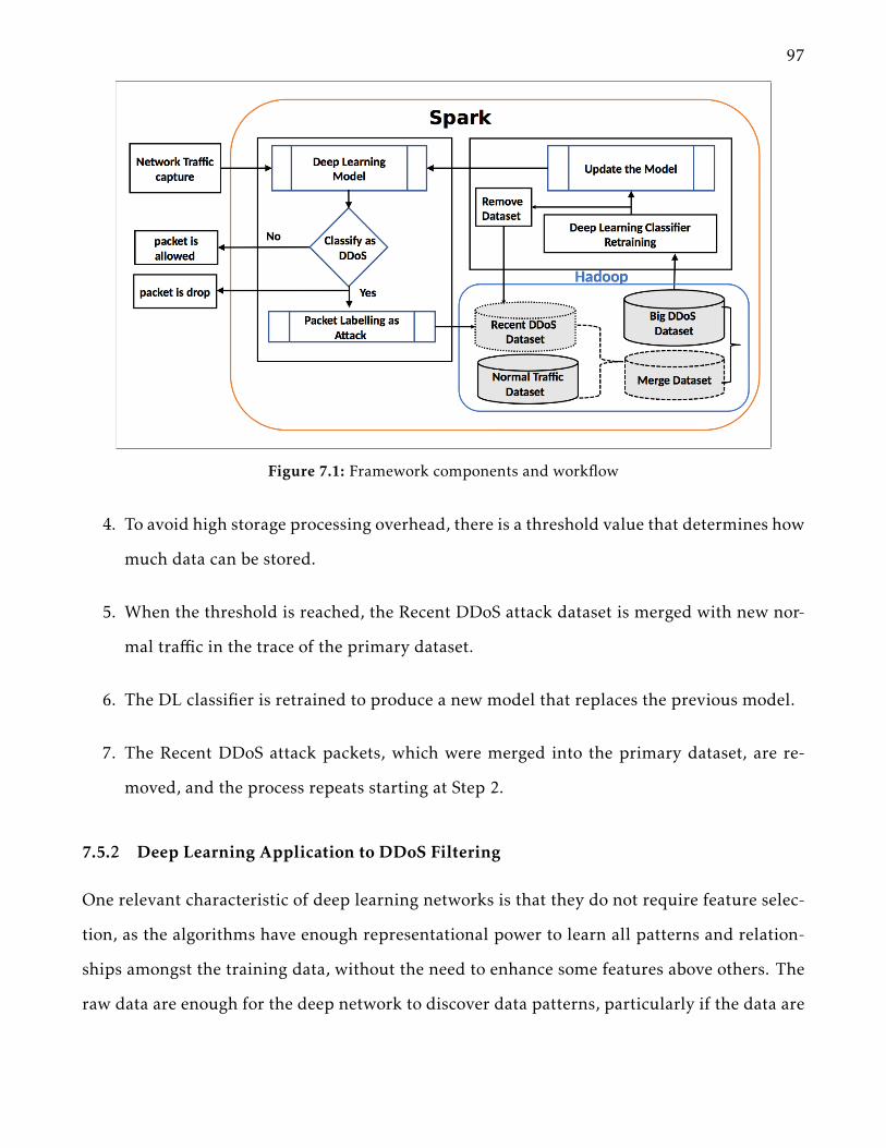
97

Figure 7.1: Framework components and workflow

4. To avoid high storage processing overhead, there is a threshold value that determines how

much data can be stored.

5. When the threshold is reached, the Recent DDoS attack dataset is merged with new nor-

mal traffic in the trace of the primary dataset.

6. The DL classifier is retrained to produce a new model that replaces the previous model.

7. The Recent DDoS attack packets, which were merged into the primary dataset, are re-

moved, and the process repeats starting at Step 2.

7.5.2 Deep Learning Application to DDoS Filtering

One relevant characteristic of deep learning networks is that they do not require feature selec-

tion, as the algorithms have enough representational power to learn all patterns and relation-

ships amongst the training data, without the need to enhance some features above others. The

raw data are enough for the deep network to discover data patterns, particularly if the data are

98

provided in large volumes.

The datasets used in the experiments have been obtained from the Center for Applied In-

ternet Data Analysis (more details are in Section 7.6.3). Most of the datasets available are not

public due to security issues, and when published (like the KDD different datasets, the UNSW-

NB15 or the CICIDS [92]), they are highly anonymized.

For this problem, an MLP approach has been selected for experimentation with different

datasets and network parameters.

An MLP, also known as a Feed Forward Network (FFN), is a network in which all its layers

are connected, and information flows from left to right. Its structure is based on using the

perceptron as the basic block to build the network by stacking perceptrons in the form of layers.

The MLP networks have several components that define the network capability to represent a

specific set of data. These components are:

1. Number of layers

2. Number of neurons in each layer

3. Activation function on each layer

There are other components that have to be defined and that affect the network behavior.

1. Cost Function

2. Optimizer algorithm for the Back-propagation phase

3. Learning rate

4. Drop percentage of connections on each layer

Other mechanisms that can be tuned for training are early stopping or dynamically changing

the learning rate. The specific parameters tested can be found in 7.6.4.

The DDoS filtering problem can be defined as a binary classification task, and the algorithm

definition for this case has some specific characteristics. The output layer will be a two neuron

99

layer, where each neuron will generate a number between 0 and 1. This two-dimensional vector

R = [x,y] will be translated into a class equation (7.1).

Class = arg max(Ri) (7.1)

The output of the Equation 7.1 is 0 or 1 (0: normal packet, 1: attack packet).

The implementation of our system has been carried out using the Elephas library [104] to

link the distributed system to the DL engines Keras and Tensorflow.

7.6 Experiments and Evaluation

7.6.1 Evaluation Methods

The evaluation was conducted in two main steps:

• Analysis of the DL algorithm performance when using different neural configurations

and different datasets sizes.

• Analysis of the DL algorithm training time and testing time.


A testbed consisting of an Apache Spark cluster, which has a master machine and three worker

node machines, was set up to examine the proposed system. All worker nodes are identical in

hardware, having a Core i7 CPU and 16 GB RAM and 500 GB of HHD, Linux Ubuntu 18.4, and

with Apache Spark and Hadoop versions 2.4.3 and 2.7.3, respectively.

7.6.3 Dataset

The original dataset containing real-world internet traffic was obtained from, CAIDA [42]. The

dataset was used to generate a binary dataset in the LIBSVM format (a format used in SPARK

clusters in which each line represents a labeled sparse feature vector). This data format has

100

the form of {xi , yi}, where i = 1.....n, in which x is a multi-dimensional input vector, and y {0,1}

represents the predicted result (0: regular traffic and 1: attack). The features were extracted

for UDP and TCP packets, respectively, using T-shark. The original dataset was duplicated

and split into seven different smaller datasets as shown in Table 7.1. The T-shark [43] was

used to extract the packets’ features from the network trace dataset. Most of the Anomaly

detection algorithms have to deal with a problem that arises from the data structure, the class

imbalance problem. This issue appears when the classes in a dataset do not have a homogeneous

distribution. The imbalance can be calculated using the following ratio [105]:

ρ =maxi(∥Ci∥)mini(∥Ci∥)

(7.2)

This ratio can be applied to multi-class datasets, and it indicates the maximum between-

class imbalance levels. In equation (7.2), Ci is a set of examples in class i, maxi(∥Ci∥) and

mini(∥Ci∥) return the maximum and minimum class sizes, respectively, calculated on all i

classes. A binary dataset which has two classes is much simpler, as it is obtained by divid-

ing the smaller class by the largest one. Table 7.1 shows the constructed datasets with the

number of rows and a quantification of the items on each class, showing the imbalance for each

one, with absolute values and a ratio ρ. The table also provides the short names (DB1, DB2,

DB3, DB4, DB5, DB6, DB7) that are used throughout the chapter to identify the datasets.

Table 7.1: Dataset sizes and class imbalance

Dataset Size Name Largest Ci Smallest Ci ρ100,000 packets DB1 85,715 14,285 0.16500,000 packets DB2 428,569 171,427 0.391 million packets DB3 857,121 142,852 0.162 million packets DB4 1,714,268 285,732 0.164 million packets DB5 2,391,579 1,608,418 0.676 million packets DB6 3,587,437 2,009,818 0.568 million packets DB7 4,783,098 3,216,902 0.67

From the analysis of the datasets, we can observe some imbalance, but, as has been noted

101

in previous works [105], the class imbalance is heavily ameliorated if the number of examples

in each class is large enough. In this application, the number of attack examples is large, thus

avoiding the issues that come from the different class representations [106].

7.6.4 Deep Learning Model Architecture

A fully connected network has been chosen as a model. It shows very good representation

capabilities with a manageable number of parameters and good training stability. A Feed For-

ward Network, also called a Multi-Layer Perceptron network, is composed of multiple fully

connected layers with different numbers of neurons in each.

Table 3.2 shows 44 dataset features that are being used to define the input layer of the

network. In the experiments, the network has shown very good accuracy and precision results

based on the following parameters.

• Depth contained in three hidden layers.

• Number of neurons: 64, 128, 258, and 512 neurons.

• Use of Exponential Linear Unit (ELU) as an activation function.

• Adam as the backpropagation optimizer.

• Binary cross-entropy as the Loss Function, which is formulated by the equation (7.3).

Binary cross-entropy is a very efficient function for binary classification. Its formulation is:

L(y, y) = − 1N

N∑

i=0

(y ∗ log(yi) + (1− y) ∗ log(1− yi)) (7.3)

In (7.3), yi denotes dataset labels and yi are the predicted labels.

Most experiments were performed using either ELU a widely used activation functions that

have good gradient transfer properties for training optimization. It is defined by equation (7.4)

102

.

ELU(z) =

⎧⎪⎪⎪⎨⎪⎪⎪⎩

z z > 0

α · (ez − 1) z <= 0

⎫⎪⎪⎪⎬⎪⎪⎪⎭(7.4)

As can be seen in the ELU definition in equation (7.4), there is a parameter α that needs to

be chosen. Both activation functions are non-linear and have shown better results than the

traditional sigmoid activation function.

7.6.5 Performance Measurements

Performance of the DL algorithm is evaluated by considering the confusion matrix, which is

one of the statistical measurements widely used in evaluating a binary classification method.

Table 3.4 shows the confusion matrix that is being used to calculate the accuracy, false-positive

rate, and the true-positive rate. The DL algorithm used 70% of the dataset for training and 30%

for testing. The training and prediction times are calculated by using timestamps.

7.7 Results

7.7.1 Neural Network Performance

Remember that we configured the deep learning with three layers in which each layer has the

same number of neurons (i.e., one of 64, 128, 258, and 512). The lower the loss, the better

the model. Figures ( A.1, A.2, A.3, A.4, A.5, A.6, and A.7 ), presented in Appendix, show the

accuracy and the loss of the training and testing (i.e., validation ) for a different number of

neurons for DB1, DB2, DB3, DB4, DB5, DB6, and DB7.

Note that in each figure, there are eight sub-figures, two for each of the networks with the

different number of neurons being 64, 128, 256, and 512 neurons. Since there are 2 subgraphs

(one for training and one for testing accuracy) for each of the number of neurons used, there

are eight subgraphs in each of the five figures.

In general, the higher the number of neurons, the higher the accuracy achieved. Noticeably,

103

the size of the dataset has a direct impact on the accuracy in which the more samples used in

the dataset, the more accurate the prediction.

It can be observed in the functions with the small datasets that training overfits due to the

lack of examples in training.

7.7.2 Classifier in ROC

Figure 7.2 shows the ROC plot for a different number of neurons in different dataset sizes.

The ROC plot represents the relationship between the False Positive Rate and the True Positive

Rate. As can be seen in Fig. 7.2, the predicted accuracy increases when training the model with

a larger dataset (i.e., the larger the dataset used to train the model, the higher the prediction

accuracy), and that it also increases within the same dataset size when the number of neurons,

or layers, increases.

7.7.3 Training Time and Testing Time analysis

Table 7.2 shows a comparison of the training times for different datasets in different neuron

configurations. Figure 7.3 shows a respective comparison view of training times. The training

time increased dramatically when the dataset size is increased.

Table 7.2: Training time in seconds

Dataset Neuron size64 128 258 512

DB1 188 195 322 812DB2 766 1561 1593 4041DB3 525 911 1932 3062DB4 1761 2016 3223 7437DB5 1928 1838 3625 10378DB6 1880 2039 5324 12024DB7 1916 5747 10709 15507

Table 7.3 shows the prediction times in seconds. Figure 7.4 shows a respective comparison

view of prediction times. The process of DDoS attack prediction requires a large number of

104

Figure 7.2: ROC view of different datasets for the same DL configuration.

packets at the same time period. Therefore, evaluating the prediction time is important to the

model’s performance. The prediction time is directly proportional to the size of the testing

dataset.

7.8 Discussion

In recent years, many researchers investigated machine learning algorithms as a solution to

DDoS attacks problems [107]. However, most of these solutions are evaluated using small

datasets [91,108,109]. Using small datasets in machine learning problems, in addition to pos-

sible overfitting, may also prevent generalization of the results [110]. Several studies have

investigated DL algorithms for a DDoS attack detection system in [17, 77–84]. In this chapter,

105

Table 7.3: Prediction time in seconds

Dataset Neuron size64 128 258 512

DB1 0.88 0.89 1.15 1.94DB2 4 5 6 20DB3 4 7 16 32DB4 17 15 30 64DB5 29 43 53 69DB6 50 42 61 156DB7 37 70 96 198

Figure 7.3: Training time comparison for different DL configuration

the main objective was to use DL for DDoS detection with a large dataset that is processed by

using Spark and Hadoop.

The results of our experimental evaluation show that the network with the highest number

of neurons (i.e., 512 neurons) not only has a high accuracy but also that its high accuracy is

achieved with fewer number of epochs. However, the model training times are higher.

106

Figure 7.4: Prediction time comparison for different DL configuration


Deep Learning in general and deep neural networks in particular, with their ability to work

with very large sets of data, are becoming relevant tools to be included in the intrusion de-

tection systems. Deep Learning systems are a good fit for DDoS detection tasks due to three

main reasons: (i) ability to represent complex relationships in the data, (ii) capability to per-

form classifications without a feature extraction process, which makes it potentially suitable to

create self-evolving systems; and (iii) capability to use and exploit massive datasets.

In this chapter, we propose a DDoS detection system based on a deep learning method

supported by a distributed cluster system. The objective is to handle large amounts of incoming

data while obtaining a powerful detection system, supported by Apache Spark and a Hadoop

cluster, in order to achieve highly accurate classification.

Different datasets with varying size are used to simulate the data training and processing.

The system accuracy, and training and the prediction times in experiments were recorded in

107

experiments and reported. The results show that the system provides higher performance when

the training dataset is larger and thus confirming our initial assumption on the importance of

dataset size for building accurate classifiers.


We implemented our system in Spark and Hadoop using YARN in the cluster mode, with the

Elephas library [104] to link the system to the DL engines Keras and Tensorflow.

1. To improve algorithm speed, the integration of one or several GPU’s in the cluster is

necessary and should be carried out in future implementations.

2. In a deep learning algorithm, many parameters have an impact on the performance. Tun-

ing these parameters is a critical phase for applying deep learning in the real world. As

the libraries used have limited support for hyperparameter searching, more sophisticated

algorithms with better hyperparameter optimization approaches, such as Bayesian opti-

mization [111], should be used.

3. As DDoS attacks evolve over time, the classification algorithm used for prediction has to

evolve as well. The development of novel techniques to allow the algorithms to identify

attacks that are not present in the training dataset is a direction of work that could bring

great benefits to the field. Applying non-supervised hybrid approaches for deep learning

can help defend assets against new types of attacks.

4. The lack of datasets for training in this area is always a concern. Owners of assets that

are targets of DDoS attacks generally prefer to avoid attacks’ publicity and are reluctant

to share the network traffic data. For this reason, the development of synthetic datasets

that could be used for training is a future area of work. Using Generative Adversarial

Networks (GANs) to generate new data, without the imbalance issue, should benefit gen-

eration of new and improved detection systems.

Chapter 8

Conclusion and Future Work

8.1 Conclusion

DDoS attacks have been launched against many organizations, resulting in severe impacts.

While researchers have been attempting to tackle DDoS attacks, the solutions put forth thus

far have not been effective against DDoS attacks. In this thesis, we enrich the field with a

number of frameworks with different objectives.

Chapter 2 of this thesis provides background of DDoS attacks and existing proposed solu-

tions. In Chapter 3, we provide background on the evaluation approach we used, including the

datasets, experiments, measurements, and distributed system we used. In Chapter 4, the thesis

presents the first proposed framework in which the GB classification algorithm and Spark dis-

tributed system were introduced. The objectives were to provide a lightweight framework that

effectively classifies traffic and can be trained quickly. The results were promising in that us-

ing the distributed system, in particular its potential for increased storage and computational

resources, can be exploited to improve the performance of classification.

In Chapter 5, we investigate a novel framework that uses fuzzy logic to dynamically select

the best classifier, from a set of prepared classifiers, to be used on incoming data stream. The

framework was evaluated in terms of accuracy achieved by the selection process and effective-

ness of the Fuzzy logic, and the results show that fuzzy logic selection is effective in leading to

improved overall accuracy.

In Chapter 6, the thesis further improves the accuracy of the classification by closely exam-

ining the dataset features in terms which features should be used for classification. A frame-

work is proposed that utilizes a number of different feature selection algorithms that are used

108

109

to improve both the adapted classification algorithms’ accuracy and to reduced the training

time. Finally, in Chapter 7, the thesis investigates the application of deep learning algorithms

to classify DDoS attacks. Although we obtain improved accuracy with deep learning, training

time delays are not the lowest. However, combining the distributed systemwith the deep learn-

ing algorithm empowers the leverage of a large dataset that should promote the generalization

of outcomes.

8.2 Future Work

Dealing with DDoS attacks is indeed a difficult problem to which many approaches have been

investigated. We investigated several novel approaches with the objective to improve the per-

formance of classifiers and reducing the training and classification delays. Our approaches

show promise in improving the performance of classification and reducing overhead delays,

but, as with other research results in this difficult problem, it does not appear that the solution

to the problem will be achieved by applying a single approach, but rather that the solution is

likely to be achieved by a careful synergistic of a number of approaches and solutions. This

is not surprising considering the increased sophistication of attacks and also the complexity

of the infrastructure in which they are launched. Thus, further research is required to obtain

improvements in performance and speed of attack detection. In this section we first offer our

opinion on future directions in terms of several key aspects that we feel need to be investi-

gated in order to gain further improvements. Following this we offer specific suggestions on

extending the frameworks proposed in this thesis.

8.2.1 Future Directions

1) It is generally accepted that increasing the size of the training dataset leads to improved

accuracy. However, increasing the size of training data also increases the requirements

on the computational and network resources. Following are specific points for future

research direction.

110

a) First, further efforts are need to obtain larger traces containing larger variety of at-

tacks so that researchers have larger volumes and variety of data to build and test

solutions. As obtaining real-attack traces is difficult due to reluctance of the victims

to release such data, the development of synthetic datasets for training is a future

area of work.

b) Further research is required on how to best exploit distributed computing approaches

in order to provide sufficient resources to process the large training and perform

classification while keeping the delays minimal for fast DDoS attack detection.

2) All approaches appear to have certain key parameters, such as thresholds, that affect the

performance and delays. Further investigation on the sensitivity of the results on such

parameters is required to build confidence in the proposed solutions.

3) Many approaches have been investigated and compared. Production ready approaches need

to be built with sufficient and reliable information describing in which conditions they

should be applied and what kind of classification performance and delays are to be ex-

pected. Furthermore, a systematic method must be developed to decide which of the

available approaches should be applied under which circumstances.

4) Feature selection has been used extensively in machine learning approaches to reduce the

size of training data in order to improve the classification performance and reduce delays.

However, the approach suffers from the risk of overfitting. Further research is required

to understand the effects of feature selection better.

5) Deep Learning approaches have become prominent and have been used in DDoS detection

systems. Further research on their application to the DDoS problem is required as the

datasets and their processing requirements are massive.

111

8.2.2 Extending Work on Frameworks

Chapter 4: The parameters of classification algorithm need to be tuned effectively. Multi-

objectives function, such as those presented in [111] may be suitable for that purpose and

should be investigated.

Chapter 5: The system evaluation was carried out in an efficient way in which a number

of aspects have been evaluated. However, we intend to conduct further research for a better

understanding of the deployment aspect.

Chapter 6: The Features Selection is an essential aspect of the machine learning training phase

for both the model performance as well as training time. Further invitations for a different FS

on this aspect is required.

Chapter 7:

1. We used Elephas [104] in distributed platform (Spark and Hadoop). However, there are

many frameworks, such as using TensorFlowOnSpark [112], that can and should be in-

vestigated for that purpose.

2. To further improve the effectiveness of distributed platform, the use of GPUs in the cluster

should be investigated.

3. As DDoS attacks evolve over time, the classification algorithm used for detection has

to evolve as well. The development of novel techniques to allow algorithms to identify

attacks that are not present in the training dataset is a direction of work for the future

that could bring potential benefits to the field.

Finally, transfer learning is an interesting area of research that can be applied. Pan and

Yang [113] have discussed most of the works of transfer learning. The idea of transfer learning

is to use earlier labelled data to present new data. The main gain with transfer learning is the

reduction in the cost of class re-labelling. Therefore, applying transfer learning is worth the

investigation to the problem.

Bibliography

[1] digital attack map website, “digital attack map.” http://www.digitalattackmap.com.Date last accessed: July 20, 2019.

[2] A. Alsirhani, S. Sampalli, and P. Bodorik, “DDoS Detection System: Utilizing GradientBoosting Algorithm and Apache Spark,” in 2018 IEEE Canadian Conference on Electrical& Computer Engineering (CCECE), pp. 1–6, IEEE, 2018.

[3] M. A. Ambusaidi, X. He, P. Nanda, and Z. Tan, “Building an intrusion detection systemusing a filter-based feature selection algorithm,” IEEE Transactions on Computers, vol. 65,pp. 2986–2998, Oct 2016.

[4] S. Aljawarneh, M. Aldwairi, and M. B. Yassein, “Anomaly-based intrusion detection sys-tem through feature selection analysis and building hybrid efficient model,” Journal ofComputational Science, vol. 25, pp. 152–160, mar 2018.

[5] A. Shameli-Sendi, M. Pourzandi, M. Fekih-Ahmed, and M. Cheriet, “Taxonomy of dis-tributed denial of service mitigation approaches for cloud computing,” J. Netw. Comput.Appl., vol. 58, pp. 165–179, Dec. 2015.

[6] N. Shone, T. N. Ngoc, V. D. Phai, and Q. Shi, “ A deep learning approach to networkintrusion detection,” IEEE Transactions on Emerging Topics in Computational Intelligence,vol. 2, no. 1, pp. 41–50, 2018.

[7] “Yahoo on Trail of Site Hackers | WIRED.” http://www.wired.com/2000/02/yahoo-on-trail-of-site-hackers/. Date last accessed: June 2, 2017.

[8] Powerful, “Powerful attack cripples majority of key Internet computers.”http://www.securityfocus.com/news/1400. Date last accessed: June 2, 2016.

[9] Mydoom, “Mydoom lesson: Take proactive steps to prevent DDoS attacks | Com-puterworld.” http://www.computerworld.com/article/2574799/security0/mydoom-lesson–take-proactive-steps-to-prevent-ddos-attacks.html. Date last accessed: June 2,2017.

[10] “Operation Payback cripples MasterCard site in revenge for WikiLeaks ban | Media |The Guardian.” http://www.theguardian.com/media/2010/dec/08/operation-payback-mastercard-website-wikileaks. Date last accessed: June 2, 2016.

[11] Ally, “DDoS: Lessons from Phase 2 Attacks - BankInfoSecurity.”http://www.bankinfosecurity.com/ddos-attacks-lessons-from-phase-2-a-5420. Datelast accessed: June 2, 2016.

112

113

[12] “5 Biggest DDoS Attacks Of The Past Decade.” "https://www.abusix.com/blog/5-biggest-ddos-attacks-of-the-past-decade". Date last accessed: June 19, 2019.

[13] “ DDoS Attacks of 2017.” https://www.tripwire.com/state-of-security/featured/5-notable-ddos-attacks-2017/. Date last accessed: June 10, 2018.

[14] A. Alsirhani, S. Sampalli, and P. Bodorik, “DDoS Detection System: Using a Set of Clas-sification Algorithms Controlled by Fuzzy Logic System in Apache Spark,” IEEE Trans-actions on Network and Service Management, 2019.

[15] A. Alsirhani, S. Sampalli, and P. Bodorik, “DDoS Attack Detection System: UtilizingClassification Algorithms with Apache Spark,” in 9th IFIP International Conference onNew Technologies, Mobility and Security, NTMS 2018, Paris, France, February 26-28, 2018,pp. 1–7, 2018.

[16] K. N. Mallikarjunan, K. Muthupriya, and S. M. Shalinie, “A survey of distributed denialof service attack,” in 2016 10th International Conference on Intelligent Systems and Control(ISCO), pp. 1–6, Jan 2016.

[17] O. Igbe, O. Ajayi, and T. Saadawi, “Detecting Denial of Service Attacks Using a Combi-nation of Dendritic Cell Algorithm and the Negative Selection Algorithm,” in 2017 IEEEInternational Conference on Smart Cloud (SmartCloud), pp. 72–77, Nov 2017.

[18] R. Song and F. Liu, “Real-time anomaly traffic monitoring based on dynamic k-NNcumulative-distance abnormal detection algorithm,” In Proceedings of the 3rd Interna-tional Conference on Cloud Computing and Intelligence System IEEE, vol. 2, pp. 187–192,2014.

[19] S. Hameed and U. Ali, “Efficacy of live DDoS detection with Hadoop,” in NOMS 2016-2016 IEEE/IFIP Network Operations and Management Symposium, pp. 488–494, IEEE,2016.

[20] B. Jia, X. Huang, R. Liu, and Y. Ma, “A DDoS Attack Detection Method Based on HybridHeterogeneous Multiclassifier Ensemble Learning,” J. Electr. Comput. Eng., vol. 2017,2017.

[21] S. M. T. Nezhad, M. Nazari, and E. A. Gharavol, “A Novel DoS and DDoS Attacks De-tection Algorithm Using ARIMA Time Series Model and Chaotic System in ComputerNetworks,” IEEE Commun. Lett., vol. 20, no. 4, pp. 700–703, 2016.

[22] K. M. Prasad, A. R. M. Reddy, and K. V. Rao, “Discriminating DDoS Attack traffic fromFlash Crowds on Internet Threat Monitors ( ITM ) Using Entropy variations,” African J.Comput. ICT, vol. 6, no. 2, pp. 53–62, 2013.

[23] M. Mizukoshi and M. Munetomo, “Distributed denial of services attack protection sys-tem with genetic algorithms on Hadoop cluster computing framework,” 2015 IEEECongress on Evolutionary Computation, CEC 2015 - Proceedings, pp. 1575–1580, 2015.

114

[24] M. Bazm, R. Khatoun, Y. Begriche, L. Khoukhi, X. Chen, and A. Serhrouchni, “Maliciousvirtual machines detection through a clustering approach,” Proceedings of 2015 Inter-national Conference on Cloud Computing Technologies and Applications, CloudTech 2015,2015.

[25] R. F. Fouladi, C. E. Kayatas, and E. Anarim, “Frequency based DDoS attack detectionapproach using naive Bayes classification,” 39th Telecommun. Signal Process. (TSP), Int.Conf., pp. 104–107, 2016.

[26] J. Kim, J. Kim, H. L. T. Thu, and H. Kim, “Long short term memory recurrent neuralnetwork classifier for intrusion detection,” in 2016 International Conference on PlatformTechnology and Service (PlatCon), pp. 1–5, Feb 2016.

[27] B. Lee, S. Amaresh, C. Green, and D. Engels, “Comparative Study of Deep LearningModels for Network Intrusion Detection,” SMU Data Science Review, vol. 1, no. 1, p. 8,2018.

[28] T. A. Tang, L. Mhamdi, D. McLernon, S. A. R. Zaidi, and M. Ghogho, “Deep learningapproach for Network Intrusion Detection in Software Defined Networking,” in 2016International Conference on Wireless Networks and Mobile Communications (WINCOM),pp. 258–263, Oct 2016.

[29] C. J. Shallue, J. Lee, J. M. Antognini, J. Sohl-Dickstein, R. Frostig, and G. E. Dahl,“Measuring the Effects of Data Parallelism on Neural Network Training,” CoRR,vol. abs/1811.03600, 2018.

[30] C. Li, Y. Wu, X. Yuan, Z. Sun, W. Wang, X. Li, and L. Gong, “Detection and defense ofDDoS attack-based on deep learning in OpenFlow-based SDN,” International Journal ofCommunication Systems, vol. 31, no. 5, p. e3497, 2018.

[31] X. Yuan, C. Li, and X. Li, “DeepDefense: Identifying DDoS Attack via Deep Learning,”in 2017 IEEE International Conference on Smart Computing (SMARTCOMP), pp. 1–8, May2017.

[32] C. Yin, Y. Zhu, J. Fei, and X. He, “A Deep Learning Approach for Intrusion DetectionUsing Recurrent Neural Networks,” IEEE Access, vol. 5, pp. 21954–21961, 2017.

[33] F. Yan, Y. He, O. Ruwase, and E. Smirni, “Efficient Deep Neural Network Serving: Fastand Furious,” IEEE Transactions on Network and Service Management, vol. 15, pp. 112–126, March 2018.

[34] J. Choi, C. Choi, B. Ko, D. Choi, and P. Kim, “Detecting Web based DDoS Attack usingMapReduce operations in Cloud Computing Environment,” J. Internet Serv. Inf. Secur.,no. 8111, pp. 28–37, 2013.

[35] H. Badis, G. Doyen, and R. Khatoun, “Understanding botclouds from a system perspec-tive: A principal component analysis,” IEEE/IFIP NOMS 2014 - IEEE/IFIP Netw. Oper.Manag. Symp. Manag. a Softw. Defin. World, 2014.

115

[36] S. Lakavath and R. L. Naik, “A Big Data Hadoop Architecture for Online Analysis.,”International Journal of Computer Science and Network Security, vol. 15, no. 11, pp. 58–62,2015.

[37] Z. Chen, G. Xu, V. Mahalingam, L. Ge, J. Nguyen, W. Yu, and C. Lu, “A Cloud ComputingBased Network Monitoring and Threat Detection System for Critical Infrastructures,”Big Data Research, vol. 3, pp. 10–23, 2016.

[38] M. Frampton, Mastering apache spark. Packt Publishing Ltd, 2015.

[39] Apache, “Apache Spark™ - Lightning-Fast Cluster Computing.”https://spark.apache.org/. Date last accessed: October 10, 2017.

[40] Apache, “Welcome to Apache™ Hadoop®!.” https://hadoop.apache.org/. Date last ac-cessed: October 13, 2017.

[41] Apache, “Apache Hadoop YARN.” https://hadoop.apache.org/docs/current/hadoop-yarn/hadoop-yarn-site/YARN.html. Date last accessed: January 13, 2019.

[42] CAIDA, “The CAIDA UCSD Anonymized Internet Traces 2015 .”http://www.caida.org.xml. Date last accessed: May 15, 2017.

[43] tshark, “tshark - The Wireshark Network Analyzer 2.4.2.”https://www.wireshark.org/docs/man-pages/tshark.html. Date last accessed: Oc-tober 13, 2017.

[44] T. Fawcett and Tom, “An introduction to ROC analysis,” Pattern Recognit. Lett., vol. 27,pp. 861–874, jun 2006.

[45] M. Frampton, Mastering apache spark. Packt Publishing Ltd, 2015.

[46] T. Hastie, R. Tibshirani, and J. Friedman, “The Elements of Statistical Learning,” Math.Intell., vol. 27, no. 2, pp. 83–85, 2001.

[47] P. A. R. Kumar and S. Selvakumar, “Detection of distributed denial of service attacksusing an ensemble of adaptive and hybrid neuro-fuzzy systems,” Comput. Commun.,vol. 36, no. 3, pp. 303–319, 2013.

[48] C. Krauss, X. A. Do, and N. Huck, “Deep neural networks, gradient-boosted trees, ran-dom forests: Statistical arbitrage on the S&P 500,” Eur. J. Oper. Res., vol. 259, no. 2,pp. 689–702, 2017.

[49] S. Peter, F. Diego, F. A. Hamprecht, and B. Nadler, “Cost efficient gradient boosting,” Adv.Neural Inf. Process. Syst. 30, no. Nips 2017, pp. 1550–1560, 2017.

[50] Z. Xu, M. J. Kusner, K. Q. Weinberger, M. Chen, and O. Chapelle, “Classifier Cas-cades and Trees for Minimizing Feature Evaluation Cost,” J. Mach. Learn. Res., vol. 15,pp. 2113–2144, Jan. 2014.

116

[51] S. Touzani, J. Granderson, and S. Fernandes, “Gradient boosting machine for modelingthe energy consumption of commercial buildings,” Energy Build., vol. 158, pp. 1533–1543, 2018.

[52] I. Brown and C. Mues, “An experimental comparison of GBM algorithm for imbalancedcredit scoring data sets,” Expert Syst. Appl., vol. 39, no. 3, pp. 3446–3453, 2012.

[53] F. Zhang, B. Du, and L. Zhang, “Scene Classification via a Gradient Boosting RandomConvolutional Network Framework,” IEEE Trans. Geosci. Remote Sens., vol. 54, no. 3,pp. 1793–1802, 2016.

[54] E. Dubossarsky, J. H. Friedman, J. T. Ormerod, and M. P. Wand, “Wavelet-based gradientboosting,” Stat. Comput., vol. 26, no. 1-2, pp. 93–105, 2016.

[55] R. Tao, L. Yang, L. Peng, B. Li, and A. Cemerlic, “A case study: Using architectural fea-tures to improve sophisticated denial-of-service attack detections,” in 2009 IEEE Sympo-sium on Computational Intelligence in Cyber Security, pp. 13–18, March 2009.

[56] A. Sahi, D. Lai, Y. Li, and M. Diykh, “An Efficient DDoS TCP Flood Attack Detection andPrevention System in a Cloud Environment,” IEEE Access, vol. 5, pp. 6036–6048, 2017.

[57] B. Cui and S. He, “Anomaly Detection Model Based on Hadoop Platform and Weka In-terface,” in 2016 10th International Conference on Innovative Mobile and Internet Servicesin Ubiquitous Computing (IMIS), pp. 84–89, July 2016.

[58] R. Rivera-Lopez and J. Canul-Reich, “Construction of near-optimal axis-parallel decisiontrees using a differential-evolution-based approach,” IEEE Access, vol. PP, no. 99, pp. 1–1,2018.

[59] L. Wei, W. Luo, J. Weng, Y. Zhong, X. Zhang, and Z. Yan, “Machine Learning-Based Ma-licious Application Detection of Android,” IEEE Access, vol. 5, pp. 25591–25601, 2017.

[60] E. F. de Oliveira, M. E. de Lima Tostes, C. A. O. de Freitas, and J. C. Leite, “Voltage THDAnalysis Using Knowledge Discovery in Databases with a Decision Tree Classifier,” IEEEAccess, vol. PP, no. 99, pp. 1–1, 2017.

[61] L. Breiman, “Random Forests,” Machine Learning, vol. 45, pp. 5–32, Oct 2001.

[62] M. W. Ahmad, M. Mourshed, and Y. Rezgui, “Trees vs Neurons: Comparison betweenrandom forest and ANN for high-resolution prediction of building energy consumption,”Energy and Buildings, vol. 147, no. Supplement C, pp. 77 – 89, 2017.

[63] L. A. Zadeh, “Fuzzy sets,” in Fuzzy Sets, Fuzzy Logic, And Fuzzy Systems: Selected Papersby Lotfi A Zadeh, pp. 394–432, World Scientific, 1996.

[64] A. Alomari, W. Phillips, N. Aslam, and F. Comeau, “Dynamic Fuzzy-Logic Based PathPlanning for Mobility-Assisted Localization in Wireless Sensor Networks,” Sensors,vol. 17, p. 1904, aug 2017.

117

[65] R. Logambigai and A. Kannan, “Fuzzy logic based unequal clustering for wireless sensornetworks,” Wireless Networks, vol. 22, pp. 945–957, Apr 2016.

[66] A. Alsirhani, S. Sampalli, and P. Bodorik, “DDoS Attack Detection System: UtilizingClassification Algorithms with Apache Spark,” in 2018 9th IFIP International Conferenceon New Technologies, Mobility and Security (NTMS), pp. 1–7, Feb 2018.

[67] X. Z. Wang, E. C. C. Tsang, and D. S. Yeung, “A problem of selecting optimal subset offuzzy-valued features,” in Systems, Man, and Cybernetics, 1999. IEEE SMC ’99 ConferenceProceedings. 1999 IEEE International Conference on, vol. 3, pp. 361–366 vol.3, 1999.

[68] W. Wang and S. Gombault, “Efficient detection of DDoS attacks with important at-tributes,” in 2008 Third International Conference on Risks and Security of Internet and Sys-tems, pp. 61–67, Oct 2008.

[69] J. C. Debuse and V. J. Rayward-Smith, “Feature Subset Selection within a Simulated An-nealing Data Mining Algorithm,” Journal of Intelligent Information Systems, vol. 9, pp. 57–81, Jul 1997.

[70] N. Chaikla and Y. Qi, “Feature Selection Using the Domain Relationship with GeneticAlgorithms,” Knowledge and Information Systems, vol. 1, pp. 377–390, Aug 1999.

[71] O. Osanaiye, K.-K. R. Choo, and M. E. Dlodlo, “Analysing Feature Selection and Classi-fication Techniques for DDoS Detection in Cloud,” in Southern Africa TelecommunicationNetworks and Applications Conference (SATNAC) 2016, pp. 198–203, 09 2016.

[72] R. Zuech and T. M. Khoshgoftaar, “A survey on Feature Selection for Intrusion detec-tion,” in Proceedings of the 21st ISSAT International Conference on Reliability and Qualityin Design, pp. 150–155, 2015.

[73] J. C. Ang, A. Mirzal, H. Haron, and H. N. A. Hamed, “Supervised, unsupervised, andsemi-supervised feature selection: a review on gene selection,” IEEE/ACM transactionson computational biology and bioinformatics, vol. 13, no. 5, pp. 971–989, 2015.

[74] M. Barati, A. Abdullah, N. I. Udzir, R. Mahmod, and N. Mustapha, “Distributed Denial ofService detection using hybrid machine learning technique,” in 2014 International Sym-posium on Biometrics and Security Technologies (ISBAST), pp. 268–273, IEEE, 2014.

[75] X. Yang, Q. Wang, and Y. Wang, “Feature selection based on network maximal correla-tion,” in 2017 20th International Symposium on Wireless Personal Multimedia Communica-tions (WPMC), pp. 448–452, IEEE, 2017.

[76] Z. Wu, C. Wang, and H. Zeng, “Research on the comparison of Flood DDoS and Low-rateDDoS,” in 2011 International Conference on Multimedia Technology, pp. 5503–5506, IEEE,2011.

[77] E. Balkanli, A. N. Zincir-Heywood, and M. I. Heywood, “Feature selection for robustbackscatter DDoS detection,” in 2015 IEEE 40th Local Computer Networks ConferenceWorkshops (LCN Workshops), pp. 611–618, Oct 2015.

118

[78] M. Barati, A. Abdullah, N. I. Udzir, R. Mahmod, and N.Mustapha, “Distributed Denial ofService detection using hybrid machine learning technique,” in 2014 International Sym-posium on Biometrics and Security Technologies (ISBAST), pp. 268–273, Aug 2014.

[79] C. Y. Tseung and K. P. Chow, “Forensic-Aware Anti-DDoS Device,” in 2018 IEEE Securityand Privacy Workshops (SPW), pp. 148–159, May 2018.

[80] R. Doshi, N. Apthorpe, and N. Feamster, “Machine Learning DDoS Detection for Con-sumer Internet of Things Devices,” in 2018 IEEE Security and Privacy Workshops (SPW),pp. 29–35, May 2018.

[81] Y. Feng, H. Akiyama, L. Lu, and K. Sakurai, “Feature Selection for Machine Learning-Based Early Detection of Distributed Cyber Attacks,” in 2018 IEEE 16th Intl Conf onDependable, Autonomic and Secure Computing, 16th Intl Conf on Pervasive Intelligence andComputing, 4th Intl Conf on Big Data Intelligence and Computing and Cyber Science andTechnology Congress(DASC/PiCom/DataCom/CyberSciTech), pp. 173–180, Aug 2018.

[82] A. R. Yusof, N. I. Udzir, A. Selamat, H. Hamdan, and M. T. Abdullah, “Adaptive featureselection for denial of services (DoS) attack,” in 2017 IEEE Conference on Application,Information and Network Security (AINS), pp. 81–84, IEEE, 2017.

[83] A. Harbola, J. Harbola, and K. S. Vaisla, “Improved Intrusion Detection in DDoS Apply-ing Feature Selection Using Rank amp;amp;amp; Score of Attributes in KDD-99 DataSet,” in 2014 International Conference on Computational Intelligence and CommunicationNetworks, pp. 840–845, Nov 2014.

[84] C. Wang, J. Zheng, and X. Li, “Research on ddos attacks detection based on rdf-svm,” in2017 10th International Conference on Intelligent Computation Technology and Automation(ICICTA), pp. 161–165, Oct 2017.

[85] P. T. Htun and K. T. Khaing, “Detection model for daniel-of-service attacks using randomforest and k-nearest neighbors,” International Journal of Advanced Research in ComputerEngineering & Technology (IJARCET), vol. 2, no. 5, pp. 1855–1860, 2013.

[86] “Chi-Squared Tests.” http://hamelg.blogspot.com/2015/11/python-for-data-analysis-part-25-chi.html. Date last accessed: January 12, 2019.

[87] Chi, “Chi Square test for feature selection.” http://www.learn4master.com/machine-learning/chi-square-test-for-feature-selection. Date last accessed: January 12, 2019.

[88] K. Wuensch, Chi-Square Tests, pp. 252–253. Berlin, Heidelberg: Springer Berlin Heidel-berg, 2011.

[89] I. Guyon and A. Elisseeff, “An introduction to variable and feature selection,” Journal ofmachine learning research, vol. 3, no. Mar, pp. 1157–1182, 2003.

[90] C. Li, Y. Wu, X. Yuan, Z. Sun, W. Wang, X. Li, and L. Gong, “Detection and defense ofDDoS attack–based on deep learning in OpenFlow-based SDN,” International Journal ofCommunication Systems, vol. 31, no. 5, p. e3497, 2018.

119

[91] A. A. Diro and N. Chilamkurti, “ Distributed attack detection scheme using deep learn-ing approach for Internet of Things,” Future Generation Computer Systems, vol. 82,pp. 761–768, 2018.

[92] R. Vinayakumar, M. Alazab, K. P. Soman, P. Poornachandran, A. Al-Nemrat, andS. Venkatraman, “Deep Learning Approach for Intelligent Intrusion Detection System,”IEEE Access, vol. 7, pp. 41525–41550, 2019.

[93] Y. LeCun, Y. Bengio, and G. E. Hinton, “Deep learning,” Nature, vol. 521, no. 7553,pp. 436–444, 2015.

[94] D. Silver, J. Schrittwieser, K. Simonyan, I. Antonoglou, A. Huang, A. Guez, T. Hubert,L. Baker, M. Lai, A. Bolton, Y. Chen, T. Lillicrap, F. Hui, L. Sifre, G. van den Driessche,T. Graepel, and D. Hassabis, “Mastering the game of Go without human knowledge,”Nature, vol. 550, pp. 354 EP –, Oct 2017. Article.

[95] J. Deng, W. Dong, R. Socher, L. Li, Kai Li, and Li Fei-Fei, “ImageNet: A large-scale hier-archical image database,” in 2009 IEEE Conference on Computer Vision and Pattern Recog-nition, pp. 248–255, June 2009.

[96] A. Krizhevsky, I. Sutskever, and G. E. Hinton, “ImageNet Classification with Deep Con-volutional Neural Networks,” in Advances in Neural Information Processing Systems 25(F. Pereira, C. J. C. Burges, L. Bottou, and K. Q. Weinberger, eds.), pp. 1097–1105, CurranAssociates, Inc., 2012.

[97] T. Young, D. Hazarika, S. Poria, and E. Cambria, “Recent Trends in Deep Learning BasedNatural Language Processing,” CoRR, vol. abs/1708.02709, 2017.

[98] G. E. Hinton, “Learning Multiple Layers of Representation,” Trends in Cognitive Sciences,vol. 11, no. 10, pp. 428–434, 2007.

[99] I. Goodfellow, Y. Bengio, and A. Courville, Deep Learning. MIT Press, 2016.

[100] P. Mishra, V. Varadharajan, U. Tupakula, and E. S. Pilli, “A Detailed Investigation andAnalysis of Using Machine Learning Techniques for Intrusion Detection,” IEEE Commu-nications Surveys Tutorials, vol. 21, pp. 686–728, Firstquarter 2019.

[101] ISCX, “UNB ISCX intrusion detection evaluation DataSet.”https://www.unb.ca/cic/about/index.html. Date last accessed: August 1, 2019.

[102] A. Saied, R. E. Overill, and T. Radzik, “Detection of known and unknown DDoS attacksusing Artificial Neural Networks,” Neurocomputing, vol. 172, pp. 385 – 393, 2016.

[103] C. Hsieh and T. Chan, “Detection DDoS attacks based on neural-network using ApacheSpark,” in 2016 International Conference on Applied System Innovation (ICASI), pp. 1–4,May 2016.

[104] “Elephas: Distributed Deep Learning with Keras & Spark.”https://github.com/maxpumperla/elephas. Date last accessed: August 1, 2019.

120

[105] M. Buda, A. Maki, and M. A. Mazurowski, “A systematic study of the class imbalanceproblem in convolutional neural networks,” Neural Networks, vol. 106, pp. 249 – 259,2018.

[106] J. M. Johnson and T. M. Khoshgoftaar, “Survey on deep learning with class imbalance,”Journal of Big Data, vol. 6, no. 1, p. 27, 2019.

[107] P. Domingos, The Master Algorithm: How the Quest for the Ultimate Learning Machine WillRemake Our World. New York, NY, USA: Basic Books, Inc., 2018.

[108] H. A. Nguyen and D. Choi, “ Application of DataMining to Network Intrusion Detection:Classifier Selection Model,” in Challenges for Next Generation Network Operations and Ser-vice Management (Y. Ma, D. Choi, and S. Ata, eds.), (Berlin, Heidelberg), pp. 399–408,Springer Berlin Heidelberg, 2008.

[109] M. V. Kotpalliwar and R. Wajgi, “Classification of Attacks Using Support Vector Machine(SVM) on KDDCUP’99 IDS Database,” in 2015 Fifth International Conference on Commu-nication Systems and Network Technologies, pp. 987–990, April 2015.

[110] P. Domingos, The Master Algorithm: How the Quest for the Ultimate Learning Machine WillRemake Our World. New York: Basic Books, 2015.

[111] J. Snoek, H. Larochelle, and R. P. Adams, “Practical Bayesian optimization of machinelearning algorithms,” in Advances in neural information processing systems, pp. 2951–2959, 2012.

[112] “TensorFlowOnSpark.” https://github.com/yahoo/TensorFlowOnSpark. Date last ac-cessed: August 1, 2019.

[113] S. J. Pan and Q. Yang, “A Survey on Transfer Learning,” IEEE Transactions on Knowledgeand Data Engineering, vol. 22, pp. 1345–1359, Oct 2010.

Appendix A

A.1 Spark and Hadoop configuration

In this Section, we provide a brief instruction to configure a Spark and Hadoop cluster as well

as how to submit an application to the cluster.

A.1.1 Java Installation

Spark support three languages: Java, Python, and Scala. We choose to implement our prototype

using Java language. Below are the command lines to install Java.

Install Java

$ sudo apt−get update

$ sudo apt−get upgrade

$ sudo apt−get i n s t a l l openjdk−8− jdk

$ sudo update−a l t e r n a t i v e s −−conf ig java

A.1.2 Spark Installation

Below are the command lines to download and install Spark.

121

122

Install Spark

$ g i t clone g i t : / / github . com/apache/ incubator$

−spark . g i t

$ t a r zxvf spark −2 . 2 . 0 . tgz

$ mv spark −2.2 .0

A.1.3 Spark Configurations

Here is how to setup the Spark environment variable.

Set environment variable SPARK_HOME

$ cd \~

$ sudo nano . bashrc

# Add the next l i n e t o the end o f th e f i l e

export SPARK_HOME=" /home/Linux−User/ spark −2.2.0−bin−had$

oop2 .7/ "

123

A.1.4 Spark files system configuration

In this section, we present the spark and hadoop files system that are configured.

Configuration of core-site.xml file

<conf igura t ion>

<property>

<name> hadoop . tmp . d i r </name>

<value> /opt /hadoop_data </value>

</property>

<property>

<name>f s . de fau l t . name</name>

<value>hdfs : //192 .168 .1 .1 :9022</value>

</property>

<property>

<name>f s . defaultFS</name>

<value>hdfs : //192 .168 .1 .1 :9022</value>

</property>

<property>

<name>dfs . permissions</name>

<value>f a l s e</value>

</property>

</ conf igura t ion>

124

Configuration of hdfs-site.xml file

<conf igura t ion>

<property>

<name>dfs . r ep l i c a t i on</name>

<value>1</value>

</property>

<property>

<name>dfs . data . d i r</name>

<value>/usr / l o c a l /hadoopdata/hdfs /datanode</value>

<f i n a l>true</ f i n a l>

</property>

<property>

<name>dfs . name . d i r</name>

<value>/usr / l o c a l /hadoopdata/hdfs /namenode</value>

<f i n a l>true</ f i n a l>

</property>

</ conf igura t ion>

125

Configuration of spark-env.sh file

# ! / usr / b in / env bash

HADOOP_CONF_DIR=/usr / loca l /hadoop/ e tc /hadoop

# Options read in YARN c l i e n t mode

SPARK_EXECUTOR_INSTANCES=4

SPARK_EXECUTOR_CORES=10

SPARK_EXECUTOR_MEMORY=2G

SPARK_DRIVER_MEMORY=9G

#\−−−−−−−

JAVA_HOME=/usr / l i b /jvm/ java −8−orac l e / j r e

#\−−−−−

SPARK_MASTER_IP=192.168.1.1

Configuration of slaves file in the master machine

# A Spark worker w i l l be s t a r t e d on each o f th e l i s t e d

# machines below .

192 .168 .1 .1

126

Configuration of slaves file in the slave 1 machine

# A Spark workers w i l l be s t a r t e d on each o f th e l i s t e d

# machines below .

192 .168 .1 .1

192 .168 .1 .2

192 .168 .1 .3

. . . . . . .

. . . . . . .

Configuration of slaves file in the slave 2 machine

# A Spark workers w i l l be s t a r t e d on each o f th e l i s t e d

# machines below .

192 .168 .1 .1

192 .168 .1 .2

192 .168 .1 .3

. . . . . .

. . . . . .

A.1.5 Maven Installation and Configurations

Recall that Jar files are required to submit an application to spark cluster. In order to build a

Jar file from Java project, we install and configure Maven.

127

Maven download

$ cd /opt /

$ wget http : / /www−eu . apache . org / d i s t /maven/ma$

ven −3/3.3 .9/ b ina r i e s /apache−maven−3.3.9− bin . t a r . gz

$ sudo ta r −xvzf apache−maven−3.3.9− bin . t a r . gz

$ sudo mv apache−maven−3.3 .9 maven

Maven Installation and Configurations

$ sudo apt−get i n s t a l l maven

$ mvn −−vers ion

Create jar file

$ cd MyAppication/main/ D i r e c t o r i e s /

$ mvn package

$ mvn clean i n s t a l l

A.1.6 Open ssh-server Configurations

In order to build a cluster, we need to connect the machines with passwordless ssh connection

between Master and all node machine.

Install openssh-server

$ sudo apt−get i n s t a l l openssh−server

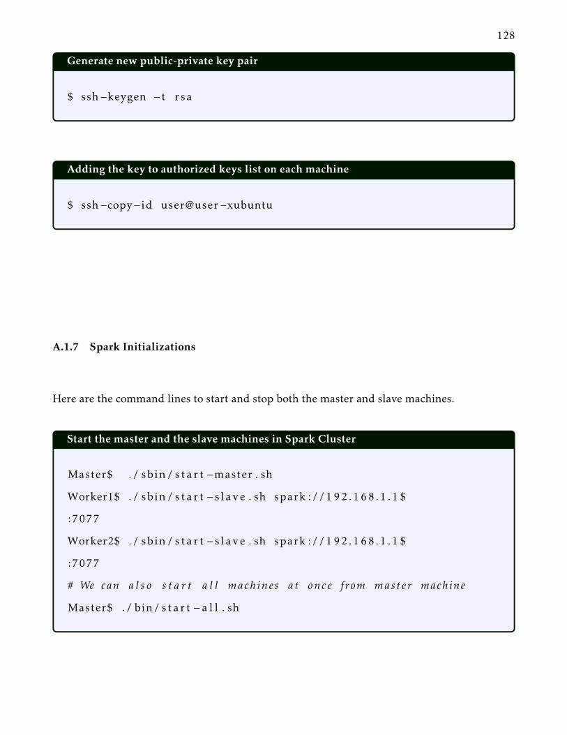
128

Generate new public-private key pair

$ ssh−keygen − t r sa

Adding the key to authorized keys list on each machine

$ ssh−copy− id user@user−xubuntu

A.1.7 Spark Initializations

Here are the command lines to start and stop both the master and slave machines.

Start the master and the slave machines in Spark Cluster

Master$ . / sbin / s t a r t −master . sh

Worker1$ . / sbin / s t a r t −s lave . sh spark : //192 .168 .1 .1 $

:7077


:7077

# We can a l s o s t a r t a l l machines a t once from master machine

Master$ . / bin / s t a r t − a l l . sh

129

Stop the master and the slave machines in Spark cluster

Master$ . / sbin / stop−master . sh

Worker1$ . / sbin / stop−s lave . sh spark : //192 .168 .1 .1 $

:7077

Worker2$ . / sbin / stop−s lave . sh spark : //192 .168 .1 .1 $

:7077

# We can a l s o s t op a l l machines a t once from master machine

Worker$ . / bin / stop− a l l . sh

A.1.8 Hadoop Initializations

Start the master and the slave machines in Hadoop cluster

Master$ . / sbin / s t a r t −master . sh

# Within node # 1


:7077

# Within node # 2


:7077

# We can a l s o s t a r t a l l machines a t once from master machine

Master$ . / bin / s t a r t − a l l . sh

130

Create dictionary in HDFS

# Crea t e d i c t i o n a r y in HDFS

$ hdfs dfs −mkdir −p /usr / loca l /hadoopdata/$

path/DictionariesName

Remove dictionary from HDFS

# Remove d i c t i o n a r y or f i l e from HDFS

$ hdfs dfs −rmr /usr / loca l /hadoopdata/hdfs /$

datanode/FileName

Copy dictionary to HDFS

# Copy data to HDFS

$ hdfs dfs −copyFromLocal − f / Source /path$

/ f i l e /Dest inat ion /path/ f i l e

A.1.9 Spark application submission

Submit an application to the cluster

$ . / bin / spark−submit −− c l a s s MainClaas −−mast$

er spark : //192 .168 .1 .1 :6066 −−deploy−mode c lu s t e r hdfs : $

/// usr / loca l /hadoopdata/hdfs /datanode/MainClaas . j a r

131

A.2 Neural Network Performance

In this section, part of the evalution of Chapter 7 are presented. Figures ( A.1, A.2, A.3, A.4,

A.5, A.6, and A.7 ) show the accuracy and loss of the training and testing (i.e., validation ) for a

different number of neurons for DB1, DB2, DB3, DB4, DB5, DB6, and DB7.

Figure A.1: Accuracy and loss function for train and test datasets of DB1.

132


133


134


135


136


137


138

A.3 List of Publications

List of Publications:

Book Chapters: •

•Alsirhani, A., Bodorik, P., & Sampalli, S. (2018). Data Fragmentation Scheme: Improving

Database Security in Cloud Computing. In Recent Trends in Computer Applications (pp.

115-138). Springer, Cham. Invited

Journals: •

•Alsirhani, A., Sampalli, S., & Bodorik, P. (2019). DDoS Detection System: Using a Set of Classi-

fication Algorithms Controlled by Fuzzy Logic System in Apache Spark. IEEE Transac-

tions on Network and Service Management.

•Alsirhani, A., Manero J., Sampalli, S., & Bodorik, P. (2019). DDoS Detection Framework: Deep

Learning in a Distributed System Cluster. IEEE Transactions on Network and Service

Management. Under Review

Conferences: •

•Alsirhani, A., Grover G., Sampalli, S., & Bodorik, P. (2019, November). Feature Selection Algo-

rithms: DDoS Detection System in a Distributed System Environment. In 2020 IEEE

Conference on Innovation in Clouds, Internet and Networks (ICIN 2020) (pp. 1-8). IEEE..

Under Review

•Alsirhani, A., Sampalli, S., & Bodorik, P. (2018, May). DDoS Detection System: Utilizing Gra-

dient Boosting Algorithm and Apache Spark. In 2018 IEEE Canadian Conference on

Electrical & Computer Engineering (CCECE) (pp. 1-6). IEEE.

•Alsirhani, A., Sampalli, S., & Bodorik, P. (2018, February). DDoS Attack Detection System: Uti-

lizing Classification Algorithms with Apache Spark. In New Technologies, Mobility and

Security (NTMS), 2018 9th IFIP International Conference on New Technologies, Mobility

& Security (NTMS) (pp. 1-7). IEEE.

139

•Alsirhani, A., Bodorik, P., & Sampalli, S. (2017, September). Improving database security in

cloud computing by fragmentation of data. In Computer and Applications (ICCA), 2017

International Conference on (pp. 43-49). IEEE.

A.4 Copyright Permission Letters

140

Title: DDoS Detection System: Using aSet of Classification AlgorithmsControlled by Fuzzy LogicSystem in Apache Spark

Author: Amjad AlsirhaniPublication: Network and Service

Management, IEEE Transactionson

Publisher: IEEEDate: Sept. 2019Copyright © 2019, IEEE

LOGINLOGIN

If you're a copyright.comuser, you can login toRightsLink using yourcopyright.com credentials.Already a RightsLink user orwant to learn more?

Thesis / Dissertation Reuse

The IEEE does not require individuals working on a thesis to obtain a formal reuse license, however,you may print out this statement to be used as a permission grant:

Requirements to be followed when using any portion (e.g., figure, graph, table, or textual material) of an IEEEcopyrighted paper in a thesis:

1) In the case of textual material (e.g., using short quotes or referring to the work within these papers) usersmust give full credit to the original source (author, paper, publication) followed by the IEEE copyright line © 2011IEEE. 2) In the case of illustrations or tabular material, we require that the copyright line © [Year of originalpublication] IEEE appear prominently with each reprinted figure and/or table. 3) If a substantial portion of the original paper is to be used, and if you are not the senior author, also obtain thesenior author's approval.

Requirements to be followed when using an entire IEEE copyrighted paper in a thesis:

1) The following IEEE copyright/ credit notice should be placed prominently in the references: © [year of originalpublication] IEEE. Reprinted, with permission, from [author names, paper title, IEEE publication title, andmonth/year of publication] 2) Only the accepted version of an IEEE copyrighted paper can be used when posting the paper or your thesison-line.3) In placing the thesis on the author's university website, please display the following message in a prominentplace on the website: In reference to IEEE copyrighted material which is used with permission in this thesis, theIEEE does not endorse any of [university/educational entity's name goes here]'s products or services. Internal orpersonal use of this material is permitted. If interested in reprinting/republishing IEEE copyrighted material foradvertising or promotional purposes or for creating new collective works for resale or redistribution, please go tohttp://www.ieee.org/publications_standards/publications/rights/rights_link.html to learn how to obtain a Licensefrom RightsLink.

If applicable, University Microfilms and/or ProQuest Library, or the Archives of Canada may supply single copiesof the dissertation.

Copyright © 2019 Copyright Clearance Center, Inc. All Rights Reserved. Privacy statement. Terms and Conditions. Comments? We would like to hear from you. E-mail us at [email protected]

141

Title: Improving Database Security inCloud Computing byFragmentation of Data

ConferenceProceedings:

2017 International Conferenceon Computer and Applications(ICCA)

Author: Amjad AlsirhaniPublisher: IEEEDate: Sept. 2017Copyright © 2017, IEEE

LOGINLOGIN










142

Title: DDoS Detection System:Utilizing Gradient BoostingAlgorithm and Apache Spark


2018 IEEE CanadianConference on Electrical &Computer Engineering (CCECE)

Author: Amjad AlsirhaniPublisher: IEEEDate: May 2018Copyright © 2018, IEEE

LOGINLOGIN










143

Title: DDoS Attack Detection System:Utilizing ClassificationAlgorithms with Apache Spark


2018 9th IFIP InternationalConference on NewTechnologies, Mobility andSecurity (NTMS)

Author: Amjad AlsirhaniPublisher: IEEEDate: Feb. 2018Copyright © 2018, IEEE

LOGINLOGIN










DDOS DETECTION MODELS USING MACHINE AND DEEP ...

Documents

Transcript of DDOS DETECTION MODELS USING MACHINE AND DEEP ...