Machine Learning and Resummation Techniques towards ...

Scuola di Dottorato in Fisica, Astrofisica e Fisica Applicata

Dipartimento di Fisica

Corso di Dottorato in Fisica, Astrofisica e Fisica Applicata

Ciclo XXXIV

Resummation and Machine Learning Techniquestowards Precision Phenomenology at the LHC

Settore Scientifico Disciplinare FIS/02

Supervisore: Prof. Stefano Forte

Coordinatore: Prof. Matteo Paris

Tesi di Dottorato di:

Tanjona R. Rabemananjara

Anno Accademico 2020-2021

This project has received funding from the European Unions Horizon 2020 research andinnovation programme under the grant agreement number 740006.

cbea Copyright Z 2021 Tanjona R. Rabemananjara, under Creative Commons Attribution-ShareAlike 4.0 International License.

Commission of the final examination:

External Referees:

Dr. Marco Bonvini INFN Sezione di Roma IDr. Riccardo Torre INFN Sezione di Genova

External Members:

Prof. Tilman Plehn Heidelberg UniversityAssoc. Prof. Juan Rojo Vrije Universiteit Amsterdam

Internal Members:

Assoc. Prof. Stefano Carrazza Universita degli Studi di Milano

Final examination:

Date: December, 20th 2021

Universita degli Studi di Milano, Dipartimento di Fisica, Milano, Italy

To my mother and Angela whom I owe everything

Internal illustrations:


Design:


Cover illustration:

Higgs diphoton events in terms of flags from the CERN 2016 Summer School

MIUR subjects:

FIS/02

KEYWORDS:

QCD, fixed-order calculations, resummation, PDFs, machine learning, GANs

ABSTRACT

The present thesis focuses on three distinct yet complementary areas in QCD. The firstarea concerns the resummation of large logarithmic contributions appearing in transversemomentum distributions. In particular, we focus on the hadroproduction of colour singletfinal states such as Higgs boson produced via gluon fusion and the production of a lepton-pair via Drell–Yan mechanism. We present phenomenological studies of a combinedresummation formalism in which standard resummation of logarithms of Q/pT is sup-plemented with the resummation of logarithmic contributions at large x=Q2/s. In sucha formalism, small-pT and threshold logarithms are resummed up to NNLL and NNLL*respectively. The second area concerns the construction of an approximate NNLO expres-sion for the transverse momentum spectra of the Higgs boson production by exploiting theanalytical structure of various resummed formulae in Mellin space. The approximationwe construct relies on the combination of two types of resummations, namely thresholdand high-energy (or small-x). Detailed phenomenological studies, both at the partonic andhadronic level, are presented. And finally, the third area concerns the a posteriori treatmentof Parton Distribution Functions (PDFs), specifically the compression of Monte Carlo PDFreplicas using techniques from deep generative models such as generative adversarialmodels (or GANs in short). We show that such a GAN-based methodology results in acompression methodology that is able to provide a compressed set with smaller numberof replicas and a more adequate representation of the original probability distribution. Thepossibility of using this methodology to address the problem of finite size effects in PDFdetermination is also investigated.

C O N T E N T S

List of Figures iiiList of Tables xiiIntroduction -1

QCD at high energies . . . . . . . . . . . . . . . . . . . . . . . . . . . . . . . . . . . -1Structure of the thesis . . . . . . . . . . . . . . . . . . . . . . . . . . . . . . . . . . . 1

I P R O L O G U E

1 PA R T O N D I S T R I B U T I O N F U N C T I O N S AT C O L L I D E R P H Y S I C S 41.1 Structure of QCD predictions . . . . . . . . . . . . . . . . . . . . . . . . . . . 4

1.1.1 Perturbative computations . . . . . . . . . . . . . . . . . . . . . . . . 41.1.2 Solving the DGLAP equations . . . . . . . . . . . . . . . . . . . . . . 161.1.3 Determination of the proton PDFs . . . . . . . . . . . . . . . . . . . . 21

1.2 Evaluating MHOUs with scale variations . . . . . . . . . . . . . . . . . . . . 251.2.1 Scale variation for partonic cross sections . . . . . . . . . . . . . . . . 251.2.2 Scale variation for parton evolutions . . . . . . . . . . . . . . . . . . . 271.2.3 Combined scale variations . . . . . . . . . . . . . . . . . . . . . . . . . 28

1.3 The road toward 1% accuracy . . . . . . . . . . . . . . . . . . . . . . . . . . . 301.3.1 Methodological aspects . . . . . . . . . . . . . . . . . . . . . . . . . . 301.3.2 Theoretical aspects . . . . . . . . . . . . . . . . . . . . . . . . . . . . . 31

1.4 Summary . . . . . . . . . . . . . . . . . . . . . . . . . . . . . . . . . . . . . . . 331.A The running of αs and asymptotic freedom . . . . . . . . . . . . . . . . . . . 331.B Integral transforms . . . . . . . . . . . . . . . . . . . . . . . . . . . . . . . . . 34

1.B.1 Fourier transform . . . . . . . . . . . . . . . . . . . . . . . . . . . . . . 341.B.2 Mellin transform . . . . . . . . . . . . . . . . . . . . . . . . . . . . . . 35

1.C Spinor Helicity Formalism . . . . . . . . . . . . . . . . . . . . . . . . . . . . . 371.D Splitting functions & Anomalous dimensions . . . . . . . . . . . . . . . . . . 40

II A TA L E O F S C A L E S

2 A L L - O R D E R R E S U M M AT I O N O F T R A N S V E R S E M O M E N T U M D I S T R I B U T I O N S 432.1 Which regions to resum? . . . . . . . . . . . . . . . . . . . . . . . . . . . . . . 432.2 Transverse momentum resummation . . . . . . . . . . . . . . . . . . . . . . . 45

2.2.1 The Collin-Soper-Sterman formulation . . . . . . . . . . . . . . . . . 452.2.2 The Catani-deFlorian-Grazzini formulation . . . . . . . . . . . . . . . 49

2.3 Threshold resummation . . . . . . . . . . . . . . . . . . . . . . . . . . . . . . 532.3.1 Resummation from renormalization-group evolution . . . . . . . . . 542.3.2 Beyond NLL resummation for colour singlet observables . . . . . . . 572.3.3 Threshold resummation and the Landau pole . . . . . . . . . . . . . 61

2.4 Soft-improved small-pT (SIPT) resummation . . . . . . . . . . . . . . . . . . 612.4.1 New factorization & Generating Functions . . . . . . . . . . . . . . . 612.4.2 Large logarithms at the level of generating functions . . . . . . . . . 632.4.3 From the generating functions to the resummed formulae . . . . . . 69

2.5 Summary . . . . . . . . . . . . . . . . . . . . . . . . . . . . . . . . . . . . . . . 73

C O N T E N T S i

2.A Process-dependent functions in Threshold resummation . . . . . . . . . . . 742.A.1 Higgs production via gluon fusion in HEFT . . . . . . . . . . . . . . 752.A.2 Vector boson production via DY mechanism . . . . . . . . . . . . . . 77

2.B Process-dependent functions in SIpT . . . . . . . . . . . . . . . . . . . . . . . 772.B.1 Higgs production via gluon fusion in HEFT . . . . . . . . . . . . . . 782.B.2 Vector boson production via DY mechanism . . . . . . . . . . . . . . 80

3 I M P R O V E D P R E D I C T I O N S F O R T R A N S V E R S E M O M E N T U M D I S T R I B U T I O N S 843.1 From Fourier-Mellin to direct space . . . . . . . . . . . . . . . . . . . . . . . . 85

3.1.1 Minimal prescription . . . . . . . . . . . . . . . . . . . . . . . . . . . . 853.1.2 PDFs in Mellin space . . . . . . . . . . . . . . . . . . . . . . . . . . . . 873.1.3 Borel prescription . . . . . . . . . . . . . . . . . . . . . . . . . . . . . . 88

3.2 Large-N behaviour at small-pT for SIPT . . . . . . . . . . . . . . . . . . . . . 933.3 Towards a combined resummation for Higgs and Drell–Yan . . . . . . . . . 96

3.3.1 SIPT in the large–b limit . . . . . . . . . . . . . . . . . . . . . . . . . . 973.3.2 Finite order truncation of the resummed expression . . . . . . . . . . 1003.3.3 Phenomenological results for SIPT . . . . . . . . . . . . . . . . . . . . 1023.3.4 Phenomenological results for the combined resummation . . . . . . 106

3.4 Approximating NNLO Higgs pT distributions using resummations . . . . . 1103.4.1 The large-N (large-x) region . . . . . . . . . . . . . . . . . . . . . . . . 1123.4.2 The small-N (small-x) region . . . . . . . . . . . . . . . . . . . . . . . 1143.4.3 Partonic level results at NLO . . . . . . . . . . . . . . . . . . . . . . . 1163.4.4 Hadronic level results . . . . . . . . . . . . . . . . . . . . . . . . . . . 119

3.5 Summary . . . . . . . . . . . . . . . . . . . . . . . . . . . . . . . . . . . . . . . 1203.A Chebyshev polynomials . . . . . . . . . . . . . . . . . . . . . . . . . . . . . . 1213.B Mellin space FO Higgs production as implemented in HPT-MON . . . . . . 122

III M A C H I N E L E A R N I N G & P D F S

4 G E N E R AT I N G N E W F E AT U R E S W I T H D E E P L E A R N I N G M O D E L S 1324.1 Basics of Deep Learning . . . . . . . . . . . . . . . . . . . . . . . . . . . . . . 1324.2 Supervised vs. Unsupervised learning . . . . . . . . . . . . . . . . . . . . . . 1364.3 Generative Models . . . . . . . . . . . . . . . . . . . . . . . . . . . . . . . . . 1374.4 Generative Neural Networks (GANs) . . . . . . . . . . . . . . . . . . . . . . 139

4.4.1 Theoretical framework . . . . . . . . . . . . . . . . . . . . . . . . . . . 1394.4.2 Challenges in training GANs . . . . . . . . . . . . . . . . . . . . . . . 1404.4.3 Training stability & Regularization . . . . . . . . . . . . . . . . . . . . 142

4.5 Summary . . . . . . . . . . . . . . . . . . . . . . . . . . . . . . . . . . . . . . . 1435 E F F I C I E N T C O M P R E S S I O N O F P D F S E T S U S I N G G A N S 145

5.1 Compression: methodological review . . . . . . . . . . . . . . . . . . . . . . 1475.2 Compressing PDF sets with GANs . . . . . . . . . . . . . . . . . . . . . . . . 151

5.2.1 The GANPDFS methodology . . . . . . . . . . . . . . . . . . . . . . . 1515.2.2 The GAN-enhanced compression methodology . . . . . . . . . . . . 156

5.3 Efficiency of the new GAN-enhanced compression . . . . . . . . . . . . . . . 1595.3.1 Validation of the GAN methodology . . . . . . . . . . . . . . . . . . . 1595.3.2 Performance of the generative-based compressor . . . . . . . . . . . 163

5.4 Phenomenological implications . . . . . . . . . . . . . . . . . . . . . . . . . . 1685.5 GANs for finite size effects . . . . . . . . . . . . . . . . . . . . . . . . . . . . . 177

ii C O N T E N T S

5.6 GANPDFS for NNPDF4.0 sets . . . . . . . . . . . . . . . . . . . . . . . . . . . 1815.7 Summary . . . . . . . . . . . . . . . . . . . . . . . . . . . . . . . . . . . . . . . 186

Conclusions 187List of Publications 217Open source softwares 218Acknowledgments 219

iii

L I S T O F F I G U R E S

Figure 1 Sample of the squared amplitudes for the tree level diagrams thatcontribute to the five-point amplitude qq → ggg. For both dia-grams, the time runs from the bottom to the top. The dashed linesthat divide the diagrams represent the Cutkosky cut [1–3]. The gluonthat is emitted collinearly to the outgoing gluon k1 is represented bythe blue-coloured coiled lines. Similarly, the soft gluon that is emittedfrom the quark p is labelled by the red-coloured coiled line. Theinternal unlabelled lines represent the outgoing gluon k2 and theincoming anti-quark q. . . . . . . . . . . . . . . . . . . . . . . . . . . 8

Figure 2 Amplitude squares arising from the virtual three-point contributionwhere two of the outgoing gluons are collinear. For both diagrams,the time runs from left to right. The dashed lines that slices bothdiagrams represent the Cutkosky cuts [1–3]. . . . . . . . . . . . . . . 11

Figure 3 Various prescriptions indicating the sampled values of the factor-ization scale κR and renormalization scale κF. From left to right, weshow the five-point prescription, the seven-point prescription, andthe nine-point prescription. The are spanned by the variation ofscales are represented by the gray shapes. The origin of coordinatescorresponds to the central scale. . . . . . . . . . . . . . . . . . . . . . 29

Figure 4 The relative parton luminosities as a function of the invariant massmX and the rapidity y for various channels, namely gg (top), gq(middle), and ud (bottom). The results are shown the the twofamilies of NNPDF sets: NNPDF3.1 (left) and NNPDF4.0 (right).The colour-bars on the right represent the relative uncertainty interms of percentage. Plots are taken from Ref. [4]. . . . . . . . . . . 32

Figure 5 Phase space available for the production of a final-state system Fwith an invariant mass M in the three kinematic limits: threshold,collinear, and high energy. The hadronic variable τ is defined interms of the center-of-mass energy

√s and the scale Q defined

according to the conventions in Sec. (1.1.1). . . . . . . . . . . . . . . 44

Figure 6 A possible path in complex Mellin space that can be chosen to eval-uate the inverse Mellin transform. The branch cut related to theLandau pole is plotted in orange while the path of the Minimal pre-scription is plotted in blue. N0 is the parameter of the integration.The path comes at some angle φ from negative complex infinity,crosses the real axis at N0, and goes to positive complex infinity ata symmetric angle. . . . . . . . . . . . . . . . . . . . . . . . . . . . . 86

iv L I S T O F F I G U R E S

Figure 7 Comparison of the baseline set NNPDF3.1 with its expansion onthe basis of the Chebyshev polynomials for the gluon and quark(s, d, d) flavours at Q2=1.65 GeV. The solid blue line represent thecentral value of the baseline PDF with the blue band representingits standard deviation 1σ-error. The dashed dark line represent theChebyshev approximation. The lower panels shows the absolutedifference, (x fcheb − x f ) /x f , between the two central values. . . . 89

Figure 8 The integral contour H that encloses the branch cut (plotted in red)and the pole at the origin ξ=0. The contour is usually taken to be acircle, here centered at ξ0=w/2 and with radius R=ξ0 + 1/2. Inpractice, we noticed that the numerical integration converge fasterif instead of a circle one considers an ellipse where the major axis ischosen to be along the real axis. . . . . . . . . . . . . . . . . . . . . . 93

Figure 9 Ratio between the terms appearing in the expansion of the re-summed expressions (standard and improved transverse momen-tum resummations) and the fixed-order results. The plot on theleft shows the ratio between the first order term in the expansionand the LO predictions, while the plot on the right shows the ratiobetween the second order term in the expansion and the secondorder term appearing in the fixed order computations. The plotswere produced with a center-of-mass energy

√s=13 TeV with a

Higgs mass mH=125 GeV. . . . . . . . . . . . . . . . . . . . . . . . . 96

Figure 10 Comparison of the Borel and Minimal Prescription for the trans-verse momentum distribution of the Higgs (left) and Z boson(right). The dashed lines represent the results of taking the large-blimit of the soft-improved transverse momentum resummation andusing the Borel method to perform the inverse Fourier transform.The solid lines represent the results from the standard resummationformalism. The renormalization (µR) and factorization (µF) scalesare set equal to the Higgs (mH) and Z boson mass (mZ) in the caseof Higgs and Z boson production respectively. The lower panelshows the ration between the two prescriptions. . . . . . . . . . . . 98

Figure 11 Normalized hadronic cross sections for different values of the cutoffC. The results are shown for different logarithmic accuracies, LL(top left), NLL (top right), and NNLL (bottom). The upper panelsshow the absolute values while the lower panel show the relativedifference between the numerical errors for each value of the cutoffand the result for the reference value C2, (dσ(Ci)− dσ(C2))/dσ(C2)for i = 2, 3, 4, 6, 10. We emphasize that the contour integration isexactly the same for all the different values of the cutoff. In thesubsequent analyses, we use as default the cutoff value C = 2. . . . 99

L I S T O F F I G U R E S v

Figure 12 Higgs transverse momentum spectra from gluon fusion at√

s =13 TeV for the two types of resummation formalisms, namely thestandard CFG (left) and the soft-improved transverse momentumresummation (right). The top panels show the pure resummedresults at various logarithmic accuracies along with the NLO fixed-order result. The lower panels show the ratio of the various pre-dictions w.r.t to the NNLL. The central scale is set to mH . Theuncertainty bands are computed using the seven-point scale varia-tion, and in all cases, Q = mH . . . . . . . . . . . . . . . . . . . . . . . 103


s =13 TeV for the two types of resummation formalisms, namely thestandard CFG (left) and the soft-improved transverse momentumresummation (right), when matched to fixed-order predictions. Thetop panels show the matched results at various logarithmic accura-cies (NLO+LO and NNLL+NLO) along with the NLO fixed-orderresult. The lower panels show the ratio of the various predictionsw.r.t to the NNLL+NLO result. The central scale is set to mH .The uncertainty bands are computed using the seven-point scalevariation, and in all cases, Q = mH . . . . . . . . . . . . . . . . . . . . 104

Figure 14 Transverse momentum spectra of the Z boson production at Teva-tron run II with

√s=1.96 TeV for the two types of resummation

formalisms, namely the standard CFG (left) and the soft-improvedtransverse momentum resummation (right). The top panels showthe pure resummed results at various logarithmic accuracies alongwith the NLO fixed-order result. The lower panels show the ratioof the various predictions w.r.t to the NNLL. The central scale is setto mZ. The uncertainty bands are computed using the seven-pointscale variation method, and in all cases, the resummation scale isfixed to Q=mZ. . . . . . . . . . . . . . . . . . . . . . . . . . . . . . . 105


√s=1.96 TeV for the two types of resummation

formalisms, namely the standard CFG (left) and the soft-improvedtransverse momentum resummation (right), when matched tofixed-order predictions. The top panels show the matched results atvarious logarithmic accuracies (NLO+LO and NNLL+NLO) alongwith the NLO fixed-order result. The lower panels show the ratio ofthe various predictions w.r.t to the NNLL+NLO result. The centralscale is set to mZ. The uncertainty bands are computed using theseven-point scale variation, and in all cases, Q=mZ. . . . . . . . . . 106

vi L I S T O F F I G U R E S


s=13 TeVfor the combined resummation formalisms. The pure resummedresults are shown on the left when the results matched to fixed-order calculations are shown on the right. The top panels showthe absolute results for the various logarithmic orders along withthe NLO fixed-order result. The lower panels show the ratio of thevarious predictions w.r.t to the NNLL (+NLO) result. The centralscale is set to mH . The uncertainty bands are computed using theseven-point scale variation, and in all cases, the resummation scaleis set to Q=mH . . . . . . . . . . . . . . . . . . . . . . . . . . . . . . . 109


√s=1.96 TeV for the combined resummation for-

malisms. The pure resummed results are shown on the left whenthe results matched to fixed-order calculations are shown on theright. The top panels show the absolute results for the various log-arithmic orders along with the NLO fixed-order result. The lowerpanels show the ratio of the various predictions w.r.t to the NNLL(+NLO) result. The central scale is set to mZ. The uncertainty bandsare computed using the seven-point scale variation, and in all cases,the resummation scale is set to Q=mZ. . . . . . . . . . . . . . . . . . 110

Figure 18 Contribution of the various (sub) channels (gg, gq, qq) to the fullhadronic cross section at the center of mass energy

√s = 13 GeV.

The full hadronic result (blue) is also for reference. The resultsare shown for both the LO (left) and NLO (right). The upperpanels show the absolute results while the lower panels show theratio between the various channels and the full hadronic result.the uncertainty bands are computed using the seven-point scalevariation method depicted in Fig. 3. In all cases the mass of theHiggs is set to mH=125 GeV. . . . . . . . . . . . . . . . . . . . . . . 112

Figure 19 Contribution of the various partonic (sub) channels (gg, gq, qq) tothe partonic cross section in Mellin space. The results are shown forthe Higgs boson production at the LHC with

√s=13 TeV for differ-

ent values of the transverse momentum, namely pT=5 GeV (top)and pT=150 GeV (bottom). The results have been computed at thecentral scale, i.e. the normalization, factorization, and resummationscales have been set to the Higgs boson mass. . . . . . . . . . . . . . 113

Figure 20 Second-order contributions of the Higgs transverse momentumdistribution at the LHC with

√s=13 TeV. The coefficient includes

the strong coupling and the Born level cross section. The fixed-order result is compared to the two different types of soft ap-proximations given in Eq. (3.4.4) and Eq. (3.4.7). The results areshown for different values of the transverse momentum, namelypT=5, 10, 90, 250 GeV. The results have been computed at the cen-tral scale, i.e. m2

H=µ2F=µ2

R. . . . . . . . . . . . . . . . . . . . . . . . 115

L I S T O F F I G U R E S vii

Figure 21 Second-order contributions of the Higgs transverse momentumdistribution at the LHC with

√s=13 TeV. The coefficient includes

the strong coupling and the Born level cross section. The fixed-order result is compared to the high-energy approximation givenin Eq. (3.4.12) and considering only the second-order terms. Theresults are shown for different values of the transverse momentum,namely pT=5, 10, 90, 250 GeV. The results have been computed atthe central scale. . . . . . . . . . . . . . . . . . . . . . . . . . . . . . . 117

Figure 22 Comparison of the second order coefficient of the Higgs transversemomentum distribution (blue) to the various approximations re-sulting from the expansion of the threshold (orange), high-energy(green), and combined threshold and high-energy resummations(red). The Higgs boson is produced via gluon fusion from a colli-sion of protons at

√s=13 GeV. The top panels show the absolute

results while the bottom panels show the ratio of the various pre-dictions to the the exact NLO. The results are shown for differentvalues of the transverse momentum, namely pT=5, 10, 90, 250 GeV. 118

Figure 23 Same as Fig. 22 but zoomed in the small-N region. . . . . . . . . . . 119Figure 24 Approximate NNLO Higgs transverse momentum distribution for

the gg-channel by combining threshold and high energy resumma-tions. The NNLO prediction is represented by the red curve. Forcomparison, the LO (blue) and NLO (green) are also shown. The toppanel represents the absolute results while the bottom panel repre-sents the relative difference between the various predictions andthe NNLO. As usual, the uncertainty bands are computed usingthe seven-point scale variation. In all the plots, the resummationscale Q is set to the Higgs mass mH . . . . . . . . . . . . . . . . . . . 120

Figure 25 An example of a multilayer perceptron model. The right networkrepresents how the input data are fed to the perceptrons, traversethrough one single hidden layer and results into a prediction ~Y.The left network describes how a perceptron is activated with aninput vector ~X, weights ~w, bias w0, and an activation function f . . . 133

Figure 26 Given a complicated distribution X , a deep generative model Gθ

is trained to map samples from a simple distribution Z definedover Rm to a more complicated distribution Gθ(Z) that is similarto X defined over Rn. If the deep generative model is inverible asis the case for Invertible Neural Networks (INNs) such as NormalizingFlows, an inverse mapping is also possible. Notice that this is notthe case for generative adversarial models. . . . . . . . . . . . . . . 137

Figure 27 Diagrammatic structure of a generative adversarial neural network.Both neural networks are represented in terms of deep convolu-tional neural networks (DCNNs). The discriminator is expressedby Dφ while the generator is expressed by Gθ . Both the true in-put data and the generated samples are fed into the discriminatorwhich evaluates whether or not the generated samples are similarto the true data. . . . . . . . . . . . . . . . . . . . . . . . . . . . . . . 140

viii L I S T O F F I G U R E S

Figure 28 Flowchart describing the methodology for the compression ofMonte Carlo PDF replicas. It takes as input a prior PDF set con-structed as a grid in (NR, n f , x)-space and additional parameterssuch as the size of the compressed set and the choice of minimiza-tion algorithm. The output is a Monte Carlo replicas with a reducedsize that follows the LHAPDF [5] grid format. . . . . . . . . . . . . . 149

Figure 29 Speed benchmark comparing the old and new compression codesusing the GA as the minimizer. The prior set is a NNPDF3.1 set withNp=1000 replicas. On the y-axis is shown the time (in minutes)that it takes to perform a compression while the x-axis representsthe various size of compressed sets. For the purpose of these bench-marks, the parameters entering the Genetic Algorithm (GA) arechosen to be exactly the same across both implementations. . . . . . 150

Figure 30 Illustration of non-convergence (left) and mode collapse (right)when generating Monte Carlo PDF replica. Here, we show the PDFfor the d-quark. The priors are represented by the green curveswhile the synthetic replicas are represented by the orange curves.The two plots we generated using the vanilla implementation ofthe generative neural network. . . . . . . . . . . . . . . . . . . . . . 152

Figure 31 Flowchart describing the GANPDFS framework. The discrimi-nator receives as input the prior PDF set computed as a grid in(Np, n f , xLHA)-points while the generator receives as input the la-tent variable constructed as Gaussian noise of linear combinationof the prior set. In addition to the real sample, the output of thegenerator also goes through the discriminator. The simoultaneoustraining of both neural networks goes on until a certain number ofepochs is reached. The final output is an enhanced PDF followingthe LHAPDF grid format. . . . . . . . . . . . . . . . . . . . . . . . . 155

Figure 32 Flowchart describing the combined GANPDFS-PYCOMPRESSOR

framework. The workflow starts with the computation of the priorMC PDF as a grid of (Np, n f , xLHA). If GAN-enhanced is required,the prior replicas are supplemented with synthetic replicas. If not,the compression follows the standard methodology. The output isalways a compressed set containing smaller numbers of replicas. . 157

Figure 33 Graphical representation of an hyperparameter scan for a few se-lected parameters. The results were produced with a certain num-ber of trial searches using the TPE algorithm. On the y-axis isrepresented the different values of the FID while the various hyper-parameters are represented on the x-axis. The violin plots representthe behaviour of the training for a given hyperparameter and vi-olins with denser tails are considered better choices due to theirstability. . . . . . . . . . . . . . . . . . . . . . . . . . . . . . . . . . . . 158

L I S T O F F I G U R E S ix

Figure 34 Histograms representing the number of disjoint replicas that arepresent in the GAN-enhanced compressed set but not in the stan-dard. That is, the green histograms are constructed by counting thenumber of replicas from the GAN-enhanced compression that arenot seen after the standard compression. Out of these numbers, thegreen histograms represent the number of replicas that are comingfrom the synthetic replicas. The results are shown as a function ofthe size of the compressed set. . . . . . . . . . . . . . . . . . . . . . . 160

Figure 35 Comparison of the PDF central values resulting from the compres-sion using the GAN-enhanced methodology for different valuesof Nc=50, 70, 100 and different PDF flavours (g, s, d, u, d). Resultsare normalized to the central value of the prior set. The 68% con-fidence interval is represented by the green hatched band wholethe 1-sigma band is represented by the dashed green lines. ThePDFs are computed at Q=1.65 GeV. Plots produced using RE-PORTENGINE-based VALIDPHYS [6] suite. . . . . . . . . . . . . . . . 161

Figure 36 Comparison of the PDF luminosities between the prior and theGAN-enhanced compressed sets at LHC with

√s=13 TeV. The

results are shown for different sizes of compressed sets, namely(Nc=50, 70, 100) and for different PDF luminosities (g-g, d-u, andd-u). The hatched error bands and the region envelopped with thedashed lines represent the 68% confidence level and 1-sigma de-viation respectively. Plots produced using REPORTENGINE-basedVALIDPHYS [6]. . . . . . . . . . . . . . . . . . . . . . . . . . . . . . . 162

Figure 37 Comparison of the best ERF values for the compression of a MonteCarlo PDF set with Np=1000 replicas for various sizes of the com-pressed sets. For each compressed set, we show the contributionof the statistical estimators (see Sec. (5.1)) that contribute to thetotal error function using the standard compression (green) andthe GAN-enhanced compression (orange) methodology. Noticethat the ERFs on the plot are non-normalized. For illustration pur-poses, the mean (purple) and median (light blue) resulting from theaverage of NR=1000 random selections are shown. The resultingconfidence intervals from the random selections are represented bythe blue (50%), green (68%), and red (90%) error bars. . . . . . . . 164

Figure 38 Comparison of the performance of the new generative-based com-pression algorithm (GANPDFS) and the previous methodology(standard). The normalized ERF values of the standard compres-sion are plotted as a function of the size Nc of the compressed set(solid black line). The dashed blue, orange, and green lines rep-resent Nc=70, 90, 100 respectively. The solid lines represent thecorresponding ERF values of the enhanced compression. . . . . . . 165

x L I S T O F F I G U R E S

Figure 39 Comparison of the correlations between various pairs of flavours.The results are shown for different size of the compressed sets,namely Nc=50, 100. The energy scale Q has been chosen to beQ=100 GeV. The correlation extracted from the results of theGAN-compressor (orange) is compared to the results from thestandard compressor (green). For a comparison, the results fromthe random selection are also shown in purple. Plots producedusing REPORTENGINE-based VALIDPHYS [6]. . . . . . . . . . . . . . 166

Figure 40 Difference between the correlation matrices of the prior and thecompressed set resulting from the standard (first row) or enhanced(second row) compression. The correlation matrices are shown fordifferent sizes of the compressed set. . . . . . . . . . . . . . . . . . . 167

Figure 41 Integrated LHC cross sections at√

s=13 TeV for W production(1st row), Z production (2nd row), top pair production (3rd row),and Higgs via VBF (4th row). The left column compares the priorwith the Nc=50 compressed sets while the right column comparesthe prior with the Nc=70 compressed sets. Plots produced usingPINEAPPL [7] scripts. . . . . . . . . . . . . . . . . . . . . . . . . . . 170

Figure 42 Differential distributions in rapidity ηX (where X=W, Z) duringthe production of a W (top) and Z bosons (bottom). The headingin each plot represents the decay mode of the corresponding weakboson. As previously, the results are shown for Nc=50 (left) andNc=70 (right). The top panels show the absolute PDFs with theseven-point scale variation uncertainties, the middle panel showthe relative uncertainties for all PDF sets, and the bottom panelsshow the pull defined in Eq. (5.4.2) between the prior and thecompressed sets generated using the standard (red) and GAN-enhanced approach (orange). Plots produced using PINEAPPL [7]scripts. . . . . . . . . . . . . . . . . . . . . . . . . . . . . . . . . . . . 172

Figure 43 Same as Fig. 42 but for top-quark pair production (top) and Higgsboson production via VBF (bottom). Similar as before, the resultsare shown for Nc=50 (left) and Nc=70 (right)Plots produced usingPINEAPPL [7] scripts. . . . . . . . . . . . . . . . . . . . . . . . . . . 173

Figure 44 The KL distance as expressed in Eq. (5.4.3) between the prior MonteCarlo PDF replicas and the compressed sets resulting from the stan-dard (green) and GAN-enhanced (orange) approach. For reference,the KL distance between the prior and its Hessian representationwith N=50 eigenvectors (blue) is also shown. For each class ofobservables, the various production modes are detailed in Table 4. . 176

Figure 45 Same as Fig. 44 but for compressed sets with Nc=70 replicas. . . . . 177

Figure 46 Positivity constraints for the prior (green) and synthetic (orange)Monte Carlo PDF replicas. The constraints correspond to the pos-itivity of a few selected observables from Eq. (14) of Ref. [8], namelyFu

2 (x, Q2), Fd2 (x, Q2), dσ2

dd/dM2dy(x1, x2, Q2), and dσ2uu/dM2dy(x1, x2, Q2).178

L I S T O F F I G U R E S xi

Figure 47 Comparison of the real and synthetic fits for various statistical esti-mators. The histograms are constructed by computing the distancebetween the two subsets of real replicas S1-S2 (green) and the dis-tance between the synthetic replicas and one of the original subsetsS1-S3 (orange). The error bars are computed by performing thedelete-1 Jackknife (left) and the bootstrap (right). In the bootstrapresampling, the results have been evaluated by performing NB=100.181

Figure 48 Same as Fig. 37 but using as a prior a Monte Carlo PDF set generatedusing the NNPDF4.0 methodology. . . . . . . . . . . . . . . . . . . 182

Figure 49 Same as Fig. 40 but using as a prior a Monte Carlo PDF set generatedusing the NNPDF4.0 methodology. . . . . . . . . . . . . . . . . . . 183

Figure 50 The left plot compares the performance of the generative-basedcompression algorithm and the standard approach. The plot onthe right represents the number of disjoint replicas that are presentin the GAN-enhanced set but not in the standard. These plots areresepectively similar to Fig. 38 and Fig. 34 with the difference thatthe prior was generated using the NNPDF4.0 methodology. . . . . 184

Figure 51 Measure of the degree of Gaussianity for all the differential distri-butions listed in Table 4. The x-axis represents the shifts betweenthe central value and the median as represented in Eq. (5.6.1) whilethe y-axis represents the shift between the standard deviation andthe 68% interval as represented in Eq. (5.6.1). The color map repre-sents the KL divergence between the priors (NNPDF3.1 top andNNPDF4.0 below) and their respective Gaussian approximations. 185

xii

L I S T O F T A B L E S

Table 1 Orders of logarithmic approximations and accuracy of the consid-ered logarithms up to NNLL. The last column represents the pre-dicted power of the logarithms upon expansion of the resummedformulae as a series in αs. In a similar way as for the Sudakov expo-nent Sc, the logarithmic contributions coming from the evolutionfactor can also be organized in terms of classes. . . . . . . . . . . . . 53

Table 2 Parameters on which the hyper-parameter scan was performed areshown in the first column. The resulting best values are shownfor both the generator and discriminator in the second and thirdcolumn respectively. . . . . . . . . . . . . . . . . . . . . . . . . . . . 159

Table 3 List of differential distributions for which the theory predictionsare computed. The distributions are all differential in the rapidityof the final-state system. For each distribution, the rapidity rangeand the number of bins are also shown. All the processes havebeen computed at the LHC energy, i.e. at a center-of-mass energy√

s=13 TeV. . . . . . . . . . . . . . . . . . . . . . . . . . . . . . . . . 169Table 4 List of differential distributions for which the theory predictions

for the Gaussian studies are computed. The distributions are alldifferential in the azimuthal angle, invariant mass, missing energy,and transverse momentum. . . . . . . . . . . . . . . . . . . . . . . . 175

Table 5 Table comparing the values of the sum rules between the real MonteCarlo replicas (prior) with Np=1000 and the synthetic replicaswith Ns=2000 generated using the GANPDFS . For each replicassample, the results are shown for the central value and the standarddeviation for the various valence quarks. . . . . . . . . . . . . . . . 179

-1

I N T R O D U C T I O N

QCD at high energies

It is now an accepted fact that most of the visible matter in the universe is composed ofhadrons. Hadrons, with the examples of protons and neutrons, are bound states of quarksand gluons. The interaction between these elementary constituents–quarks and gluons (col-lectively known as partons)–are dictated by the strong nuclear force whose mathematicaldescription is formulated in a quantum field theory known as Quantum Chromodynamics(or QCD in short). In this picture, partons carry colour charges that transform under the(anti-) fundamental and adjoint representation of the group SU(3), but which at the levelof hadrons lead to a neutral colour combination. QCD, in turns, constitutes a part ofa larger theory called Standard Model (SM) which provides a theoretical framework tothe description of all known interactions (electromagnetic, weak and strong interactions)except gravity.

One of the defining features of QCD is that as the energy grows, the elementary inter-actions taking place in a collision of hadrons occur at distances much smaller than theconfinement scale, allowing for their descriptions to be formulated in terms of quasi-freequarks and gluons. In this respect, theoretical predictions of hard scatterings are calculatedusing perturbative QCD (or pQCD). In pQCD, the observable of interest is expanded asa power series in the QCD strong coupling αs. In the case where the strong coupling issmall compared to other scales involved in the process, truncating the perturbative seriesat some finite power of αs is an accurate approximation to the full calculation. This iscrucial since the exact computation of physical observables is not feasible within the realmof QCD. To the present day, several observables that are of interests to hadron colliderssuch as LHC have been computed to very high accuracy in perturbation theory both at theintegrated [9–21] and differential [22–33] levels. Whilst pushing the frontier of currentlyknown perturbative orders seems to be a gigantic task, it is natural to extract as muchinformation as possible concerning the unknown orders from known orders. Hereinafter,we refer to this as the estimation of the missing higher-order uncertainties.

However, in order to compute measurable observables that can be compared to experi-mental measurements, the results from perturbative calculations have to be supplementedwith the knowledge of the momentum distributions of the partons inside the collidinghadrons. Such information are encapsulated in what is known as Parton DistributionFunctions (PDFs). This suggests that in order to perform precision calculations for hadron-initiated processes (henceforth referred to as hadroproduction), an accurate knowledge ofthe PDFs is crucial. As a matter of fact, not only PDFs are vital to high-precision physics atLHC, but as will be briefly discussed later, they are essential tools to interpret experimentalmeasurements for a variety of hard processes in light of the quest for new physics (beyondthe Standard Model or BSM). Since they contain information on long-distance interactions,parton distributions are non-perturbative objects, and hence they cannot be computedfrom first principle. Instead, they have to be determined through a fitting procedure inwhich theoretical predictions are compared to experimental measurements.

0 I N T R O D U C T I O N

The problem of accurately determining PDFs has seen considerable advancements inthe past decades. There exists thus far various PDF fitting groups [34–74] that implementdifferent methodology and provide different estimation of the PDF errors. Remarkably,despite the fact the resulting PDFs may differ, they agree within a reasonable uncertainty.Roughly speaking, the underpinning idea behind a PDF determination consists in learningfrom experimental data a set of functions. That is, a parton density function is modelledin terms of a function whose parameters are adjusted during the fit to yield matchingtheoretical predictions. Such a function, for instance, can be defined in terms of a suitablepolynomials whose functional form is chosen based on physical arguments such as Reggetheory [75], Brodsky-Farrar quark counting rules [76], et cetera. This approach is used by all thePDF fitting groups mentioned previously except the NNPDF. The NNPDF collaborationtakes a different approach by modelling the parton density functions in terms of neuralnetworks. This approach turns out to be very robust as it removes the bias introducedin the choice of a particular functional form to fit the PDFs. Very recently [4, 77], thanksto the adoption of state-of-the-art machine learning methodologies and the inclusion ofnew datasets, the NNPDF collaboration claims to reach–in a wide range of kinematicregions–one-percent relative uncertainties. This is a milestone toward reaching the objectiveof having smaller PDF errors, which so far represented one of the dominant sources ofuncertainties in LHC processes such as the Higgs boson production. However, in orderto consistently produce PDFs accurate at a percent-level, theoretical uncertainties [52,53] (especially those arising from missing higher-orders) have to be taken into account.Hopefully, with the current NNPDF4.0 methodology [77] and evolution codes such asEKO [78] and YADISM [79], this will become possible in the very near future.

Returning back to the short-distance interactions, perturbative computations sufferfrom two main pathologies: first the appearance of large logarithmic enhanced terms in amultiscale process even if the observable in question is Infrared and Collinear (IRC) safe,second the non-existence of a robust and reliable method to estimate missing higher-orderuncertainties. In the former, the smallness of the QCD coupling αs is compensated by thelargeness of ln µ2 (where µ denotes an arbitrary ratio of scales) such that αs ln µ2∼O(1).In such a scenario, the convergence of the perturbative series is spoiled and any truncationat a given power of αs is meaningless. These types of logarithmic divergences are cured byperforming an all-order computation through a procedure known as resummation. Generally,different resummation techniques are required for different classes of large logarithms.For instance, logarithmic enhancements arising when the invariant mass of the final-statesystem approaches the kinematic threshold are resummed in threshold resummation.

The issue related to finding an efficient method to estimate theoretical uncertainties asso-ciated with missing higher-order corrections is still arguably an open question. Currently,the most standard way to evaluate such uncertainties is by varying the unphysical scalesinvolved in the process according to a scale variation prescription. This approach, however,has a number of caveats. Various approaches have recently emerged [80–82] in order toaddress the shortcomings related to the scale variation method. However, most of theseapproaches are only applicable to particular types of processes and observables.

All of this said, in order to push forward precision and discovery physics at the LHC,the three pillars of QCD–namely the fixed-order calculations, resummations, and PDFs–need to be determined at the highest accuracy possible. While significant efforts havebeen underway at the PDF level to achieve this objective, much works remain both in

0.0 S T R U C T U R E O F T H E T H E S I S 1

terms of fixed-order computations (especially with regards to the estimation of missinghigher-order uncertainties), and resummations. The present thesis attempts to fill the tinygaps in those areas by combining theoretical computations and machine learning.

Structure of the thesis

In Chapter 1, we first establishes background notations and definitions on which the theo-retical part of the present thesis is based upon. In particular, we review how theoreticalpredictions in QCD are computed. Specifically, we briefly review how matrix elements fac-torize in the collinear and soft limits and re-derive the expression of the splitting functionsusing non-classical approach such as spinor helicity formalism and MHV techniques. Thisis followed by a description of the underlying ideas behind a PDF determination. We thenconclude the introductory part by commenting on the estimation of missing higher-orderuncertainties in fixed-order computations and the road toward one-percent accuracy.

In Chapter 2, we detail how the large logarithmic contributions appearing in perturbativecomputations due to kinematic enhancements are cured using resummation techniques inthe context of transverse momentum distributions. Specifically, we focus on the resumma-tions of contributions that are enhanced at the partonic threshold and at small transversemomentum. We then provide detailed derivations on how subclasses of the thresholdlogarithms can be consistently incorporated into the transverse momentum resummation.In doing so, we extensively study the relation between the soft and collinear logarithmswhich drive the transverse momentum distribution.

In Chapter 3, we perform extensive phenomenological studies in which the soft-improvedstandard transverse momentum resummation is compared with the standard transversemomentum resummation in the context of Higgs boson production at the LHC and Z-boson production via Drell–Yan (DY) mechanism. This eventually requires us to constructprescriptions to perform the inverse Fourier and Mellin transforms in which the resumma-tions are derived. Then, by studying the singularity structure of the resummed expressions(specifically threshold and high energy resummations), we try to construct an approxima-tion to the NNLO transverse momentum distribution of the Higgs boson produced viagluon fusion in the HEFT approximation.

In Chapter 4, we introduce machine learning concepts that are relevant for the treatmentof Monte Carlo PDF sets. For the sake of pedagogical clarity, we purposefully give a briefreview of deep learning and analyse, through explicit illustrations the mechanism behindthe training of a deep neural network. We then describe how deep learning can be usedto model posterior probability distributions. In particular, we concentrate our attention toa specific deep generative model known as Generative Adversarial Network (or GANs inshort). To conclude the chapter, we give a brief survey of how GANs have been applied sofar to tackle problems in high energy physics.

In Chapter 5, we apply the concept of GANs to the problem of compressing Monte CarloPDF sets. The need for a PDF compression can be stated as follows: the main publishedPDFs are typically based on a NR=1000 replicas fit, however, having to deal with such alarge set of replicas is not ideal when performing Monte Carlo simulations, for example.For this reason, it is therefore advantageous to construct a set of replicas with smaller sizes

2 I N T R O D U C T I O N

while maintaining the same underlying probability distribution as the prior. The role ofthe GAN is then to further enhance the statistics of a given PDF set by generating syntheticreplicas before a compression is performed. This, as will be discussed further, results in acompression methodology that is able to provide a compressed set with smaller numberof replicas and a more adequate representation of the original probability distribution.Before closing the chapter, we investigate the possibility of using the GANs to tackle finitesize effects in PDFs.

Finally, we conclude by first summarizing the main guiding ideas and results presented inthe present thesis. In particular, we highlight the relevance of resummation in perturbativecomputations and the possibility of combining different categories of resummation toconstruct approximate predictions for yet unknown higher-order contributions.

Part I

P R O L O G U E

4

1PA R T O N D I S T R I B U T I O N F U N C T I O N S A T C O L L I D E R P H Y S I C S

In the following chapter, we set the stage to the research topics studied in the presentthesis. In particular, we highlight the role the QCD factorization theorem plays in per-turbative calculations in order to separate short-distance interactions from long-distanceones. The concept of Mellin transforms is then introduced in the context of transversemomentum observables, which turns out to be crucial for all-order computations. Asvery well known in pQCD, scattering amplitudes factorize in presence of radiative (softand/or collinear) emissions. These properties are reviewed in Sec. (1.1.1) using the spinorhelicity formalism and Maximally Helicity Violating (MHV) techniques. Such computationseventually lead to the introduction of splitting functions that govern the DGLAP equations.We then explicitly show how the solutions to the DGLAP equations are computed. Sucha derivation is relevant in the context of soft-improved transverse momentum resummation(discussed in Sec. (2.4)) where the PDF evolutions need to be treated in a particular way.While the µ2-dependence of the PDFs is predicted at all values by the DGLAP equations,the x-dependence must be derived through a fit to the experimental data. Details on suchdeterminations are briefly described in Sec. (1.1.3). To conclude the chapter, we discussthe main missing pieces in terms of PDF determination and perturbative computationstoward achieving a one-percent accuracy.

1.1 Structure of QCD predictions

1.1.1 Perturbative computations

At hadron colliders such as LHC, the colliding particles are bound configurations of quarksand gluons. As mentioned in the introduction, these bound states are held together bythe strong nuclear force whose mathematical descriptions are described by the QuantumChromodynamics (or QCD in short). A proton, for example, can be thought as a boundstate of one down quark (d) and two up quarks (u)1. At high-energies (greater thanΛQCD∼200 MeV) where hadrons behave as bunches of quasi-free partons (phenomenonknown as Asymptotic Freedom), QCD effects modify the effective composition of the protonswhere they also contain gluons, and quarks & antiquarks of all flavours. In the partonmodel, interactions of hadrons taking place at such energy can be described through theinteractions of partons via the QCD factorization theorem.

1 Recent studies of the contents of the proton by the NNPDF collaboration, however, seem to suggests that thebound state of the proton also contains a charm (c) quark. This is thought to be the case due to the presence abump in the charm-quark distribution at x∼0.3

1.1 S T R U C T U R E O F Q C D P R E D I C T I O N S 5

Hadron collisions & QCD factorization theorem

Physical processes (specifically hadroproduction) typically studied at hadron colliders takeplace at very high energies2 allowing for the separation of the long-distance physics and theshort-distance ones. The assumption of the parton model states that physical observablescan be computed in terms of perturbative objects such as partonic cross sections. Thus, fora collision of two hadrons h1 and h2 leading to the creation of a final-state system F, anobservable O (typically cross section) can be factorized as follows

O = ∑a,b

fa/1(µ)⊗ fb/2(µ)⊗ Oab(µ), (1.1.1)

where the sum takes into account all the possible sub-partonic channels and ⊗ denotesthe convolution. The function fa/h represents the Parton Distribution Function (PDF)and describes the fraction of momentum carried out by a parton a from a hadron h. Thepartonic version of the physical observable is represented by O. The scale µ–conventionallyknown as factorization scale–separates soft (long-distance) and hard (short-distance) physics.As physical quantities should not depend on the scale µ, Eq. (1.1.1) suggests that the scaledependence must cancel when the perturbative part is convoluted with the PDFs. However,in perturbative computations, only a few orders in the strong coupling are included in O ,leaving the scale dependence present. Based on renormalization group invariance, such ascale dependence is, however, expected to decrease as the perturbative order increases. Asa result, the residual scale dependence µ is typically used to estimate the size of the nextunknown contribution in the perturbative expansion.

The PDFs, as opposed to the hard scattering part, are process-agnostic. They cannotbe computed using perturbative QCD and therefore needs to be extracted from experi-mental data using some fitting procedure. In order for the PDFs to have a probabilisticinterpretation, they need to satisfy a set of constraints known as sum rules. In other words,PDFs are constrained such that integrating a parton PDF over all the momentum fractionx must yield the number of valence partons present in the hadron. For instance, a protonmust be composed of one valence down quark and two valence up quarks. In addition, for theremaining quark flavours (`=s, c, b, t), the valence must be equal to zero as these quark-antiquark pairs fluctuate in and out of existence within the proton. These constraints canbe mathematically written as

∫ 1

0dx ( f`(x)− f ¯(x)) = 0,

∫ 1

0dx ( fd(x)− fd(x)) = 1,

∫ 1

0dx ( fu(x)− fu(x)) = 2.

(1.1.2)

Since there is no number conservation law for gluons, gluons are only constrained bymomentum conservation, i.e. satisfy ∑i

∫x fi(x)=1 where i sums over the gluon and all

quark & antiquark flavours.The factorization formula given in Eq. (1.1.1) thus far has only been rigorously proven for

sufficiently inclusive observable such as Deep Inelastic Scatterings (DIS) and its validity formore exclusive observables remain to be proved (especially at higher perturbative order).That is, for most of the physical observables that are of interests to LHC phenomenology,

2 The Run II of the LHC, for examples approached a center-of-mass energy of√

s∼14 TeV.

6 PA R T O N D I S T R I B U T I O N F U N C T I O N S AT C O L L I D E R P H Y S I C S

such as differential distributions, the factorization theorem is simply assumed to holdtrue. In addition, Eq. (1.1.1) is only valid up to power corrections O

(ΛQCD/Q

)therefore

neglecting hadronization corrections and higher-twist contributions which at the energyconsidered in this thesis are negligible.

Let us make a final comment on the partonic component of Eq. (1.1.1). As mentionedbefore, the hard parton scattering O can be computed using perturbative approach. Inthe presence of collinear emission in either the initial or final sate, it exhibits collineardivergences. Such divergences can be factorized out from the hard scattering as

Oab(µ) = ∑i,jCi/a(µ)⊗ Cj/b(µ)⊗ Oij (1.1.3)

where Ci/a are referred to as collinear counter-terms describing the singular part of theparton-in-parton distribution due to higher order corrections to the parton a. In the casewhere the observable we are considering is both Infrared and Collinear Safe (IRC safe), thefunctions Ci/a and Oij are well defined (finite) perturbative functions. Details on thissubject are explored in the subsequent sections.

Notations & Definitions for transverse momentum distributions

Consider the collision of two protons p1+p2 −→ F+X in which a colour singlet object Fis produced with an invariant mass M and transverse momentum pT . We can define ascaling variable τ as follows

τ =(ET + pT)

2

s(1.1.4)

where s=(p1+p2)2 represent the hadronic center-of-mass energy squared. The analogue

of τ and s at the partonic level is given by

x =(ET + pT)

2

swhere ET =

√M2 + p2

T and s = x1x2s (1.1.5)

with x1 and x2 representing the momentum fractions. By introducing a new variableQ=ET + pT , the hadronic and partonic scaling variables become τ=Q2/s and x=Q2/srespectively. Here, Q is the threshold energy, i.e. the minimum energy needed to producethe final state system F with an invariant mass M. This ensures that 0≤τ≤1. Using thefactorization formula given in Eq. (1.1.1), the hadronic cross section for the transversemomentum distribution can be written as

1τ

dσ

dξp

(τ,

M2

Q2 ,M2

µ2R

,M2

µ2F

)= ∑

a,b

∫ dxxLab

(τ

x, µ2

F

) 1x

dσabdξp

(x,

M2

Q2 ,M2

µ2R

,M2

µ2F

)(1.1.6)

where we have defined the dimensionless variable ξp= p2T/M2. For brevity, we have

omitted the explicit dependence on the strong coupling αs. It should always be kept inmind that dσab/dξp is a perturbative function admitting a series expansion in αs. Theluminosity function Lab is expressed in terms of the two parton densities as

Lab

(z, µ2

F

)=∫ 1

z

dyy

fa(y) fb

(zy

). (1.1.7)


In the context of all-order computations, it is clear that Eq. (1.1.6) is not suitable due tothe presence of convolution. However, it turns out that in Mellin space, the convolutionbecomes a normal product. The Mellin transform of Eq. (1.1.6) can be constructed bydefining the following transformations

dσ

dξp

(N,

M2

Q2 ,M2

µ2R

,M2

µ2F

)=∫ 1

0dτ τN−1 dσ

dξp

(τ,

M2

M2 ,M2

µ2R

,M2

µ2F

)(1.1.8)

dσ

dξp

(N,

M2

Q2 ,M2

µ2R

,M2

µ2R

)=∫ 1

0dx xN−1 dσ

dξp

(x,

M2

Q2 ,M2

µ2R

,M2

µ2F

). (1.1.9)

Using Eq. (1.1.8) and Eq. (1.1.9), it can be shown that Eq. (1.1.6) can be written as

dσ

dξp

(N,

M2

Q2 ,M2

µ2R

,M2

µ2F

)= ∑

a,bLab

(N + 1, µ2

F

) dσabdξp

(N,

M2

Q2 ,M2

µ2R

,M2

µ2F

). (1.1.10)

Notice that the cross sections and their Mellin transforms are denoted with the samesymbol and only distinguished through their arguments. It is worth emphasizing thatthe Mellin transform of the hadronic cross section in Eq. (1.1.8) is taken w.r.t. the scalingvariable τ while the Mellin transform of the hard partonic cross section in Eq. (1.1.9) istaken w.r.t. the partonic variable x.

Matrix element factorization in the collinear limit

To see how matrix elements factorize in the collinear limit, let us consider a 2 to 3 processwhere two of the outgoing particles are collinear. In particular, let us consider a processin which a quark and an antiquark annihilates and produces three gluons (qq→ ggg), asdepicted in Fig. 1. Using the spinor helicity formalism, each momentum involved in theprocess can be expressed in terms of a left and right-handed spinors kaa=λaλa (where aand a are spinor indices running from 1 to 2). For real-valued momenta, the holomorphicand anti-holomorphic spinors (λa and λa respectively) are complex conjugate of each other,λ?

a = λa. In such a representation, massless tree-level amplitudes are straightforwardlycomputed by considering all the momenta to be either incoming or outgoing in which theleading non-vanishing contribution is given by the Maximally Helicity Violating (MHV)amplitudes [83–86]. By virtue of the colour kinematic decomposition [87–91], the fullamplitude for a given helicity configuration of a process involving three gluons and aquark-antiquark pair is given by

M5 (p, 1, 2, 3, p) = g3s ∑P3

(Ta1 Ta2 Ta3) M5 (p, 1, 2, 3, p) (1.1.11)

where P3 sums over the permutations of all three gluons, gs is the fine structure constant(g2

s =4παs), Ta are the generator matrices of SU(3), and M are called colour-ordered partialamplitudes which have all the colour factors removed. It is worth emphasizing that eachpartial amplitude corresponds to a particular colour flow, which naively can be thought asthe ordering in which the gluons are emitted. Let us first consider an MHV configurationin which only the quark p and gluon k1 possess negative helicities. Using the Parke-Taylor


k1 k1

p p

k1 k1

p p

Figure 1 Sample of the squared amplitudes for the tree level diagrams that contribute tothe five-point amplitude qq→ ggg. For both diagrams, the time runs from the bottom tothe top. The dashed lines that divide the diagrams represent the Cutkosky cut [1–3]. Thegluon that is emitted collinearly to the outgoing gluon k1 is represented by the blue-colouredcoiled lines. Similarly, the soft gluon that is emitted from the quark p is labelled by thered-coloured coiled line. The internal unlabelled lines represent the outgoing gluon k2 andthe incoming anti-quark q.

formula [92] (see discussions in App. 1.C), the MHV colour-ordered amplitude for ourfive-point process is given by the following expression

M5(

p−, 1−, 2+, 3+, p+)=

〈p1〉3〈 p1〉〈p1〉〈12〉〈23〉〈3p〉〈 pp〉 (1.1.12)

where the angle brackets are defined in terms of the scalar product of two momenta as2(kik j)=

(εabλaµb

) (εabλaµb

)=〈ij〉 [ij]. Therefore, the angle and square brackets repre-

sentation of the spinors are defined as 〈ij〉=εabλaµb and [ij] =εabλaµb. Hereinafter, wedrop the dependence on p and p and only keep M5 (1−, 2+, 3+). Indeed, due to the parityof the partial amplitudes, the helicity of the quark-antiquark line is immaterial and oneonly has to take into account in the full amplitude configurations where the helicities ofthe gluons change.

In the limit where the two gluons k2 and k3 are collinear, the spinor products 〈23〉 and[23] vanish. This can be used to simplify further the expression of the full amplitudesince in this limit only terms that contain 〈23〉 and/or [23] in the denominator contribute.That is, the partial amplitudes M5 (1−, 2+, 3+) and M5 (2−, 3+, 1+) will contribute to thefull amplitude while partial amplitudes with helicity configurations M5 (2−, 1+, 3+) andM5 (3−, 1+, 2+) will be suppressed. Introducing an intermediate momentum q=(k2+k3),the collinearity condition implies that k2=xq and k3=(1−x)q where x is the fraction ofmomentum carried out by the gluon k2. Defining the momenta to be q=µaµa, k2=λaλa,and k3=ηaηa, the aforementioned parametrization can be translated into spinor variablesas follows

{λa =

√xµa

λa =√

xµa, and

{ηa =

√1− xµa

ηa =√

1− xµa.(1.1.13)


Plugging the above relations into Eq. (1.1.12) and exploiting the linearity of the angle brack-ets in order to factorize the fraction of momentum x, we can write the partial amplitudefor the helicity configuration M5 (1−, 2+, 3+) as follows

M5(1−, 2+, 3+

)=

1〈23〉

√x(1− x)

〈p1〉3〈 p1〉〈p1〉〈1q〉〈qp〉〈 pp〉 , (1.1.14)

where we have made explicit the term coming from the four-point partial amplitudeM4 (1−, q+). Indeed, it is clear from Eq. (1.1.14) that in the collinear limit, the MHVamplitude for the helicity configuration considered factorizes into a four-point part anda collinear term, M5∼ f (2, 3, x)M4. The same exact calculations can be performed forall possible helicity configurations that lead to non-vanishing partial amplitudes. Forcompleteness, we list the two remaining MHV configurations below

M5(1+, 2−, 3+

)=

x2

〈23〉√

x(1− x)M5

(1+, q−

)(1.1.15)

M5(1+, 2+, 3−

)=

(1− x)2

〈23〉√

x(1− x)M5

(1+, q−

). (1.1.16)

Notice that the anti-MHV partial amplitudes can be straightforwardly computed fromthe MHV configurations by realizing that M ({hi}) and M ({−hi}) (with hi denoting thehelicity) are related by a change of angle brackets into square brackets. That is,

M5(1+, 2−, 3−

)=

1[23]

√x(1− x)

M5(1+, q−

)(1.1.17)

M5(1−, 2+, 3−

)=

x2

[23]√

x(1− x)M5

(1−, q+

)(1.1.18)

M5(1−, 2−, 3+

)=

(1− x)2

[23]√

x(1− x)M5

(1−, q+

)(1.1.19)

In order to complete the computation of the full amplitude, for say the configuration(1−, 2+, 3+), we need to consider all the possible permutations of gluons as expressedin Eq. (1.1.11). This can be effortlessly done by realizing that: (a) due to the cyclic orderingof the gluons the partial amplitude M5 (2, 3, 1) is related to M5 (1, 2, 3) by a swap of k1and q in the four-point partial amplitude, (b) due to the antisymmetric property of theangle and square brackets M5 (1, 2, 3) and M5 (1, 3, 2) are related by an overall minussign. Combining these observations and exploiting the normalization of the generatormatrices [Ta, Tb] = fabcTc, we can finally write down the expression of the full amplitudefor the helicity configuration (1−, 2+, 3+)

M5(1−, 2+, 3+

)= − gs fa2a3c

〈23〉√

x(1− x)∑P2

(Ta1 Tc) M4(1−, q+

), (1.1.20)

where P2 sums over the permutation of the two gluons k1 and q. We can now take themodulus square of the above amplitude and sum over the colours by promoting thegenerator matrices to structure constants and finally using ∑ fa2a3c fa2a3d=CAδcd. Doing


so leads to an expression where the collinear term and the four-point amplitude areindependent of each other

∣∣M5(1−, 2+, 3+

)∣∣2 =g2

s2(k2k3)

CAx(1− x)

∣∣M4(1−, q+

)∣∣2 (1.1.21)

The final step consists in summing the square amplitudes (as in Eq. (1.1.21)) over all thepossible helicity configurations (including MHV). Provided with Eqs. (1.1.15-1.1.19), thisjust amounts to a few algebraic simplifications. The final expression now writes as

∑hel.|M5 (1, 2, 3)|2 = αs

(4π

q

)2P(0)

gg (x) ∑hel.|M4 (1, q)|2 , (1.1.22)

where we have defined the leading-order Altarelli-Parisi splitting function associated withthe probability of the gluon to split into two gluons (g→ gg) to be

P(0)gg (x) =

CAπ

[x

1− x+

1− xx

+ x(1− x)]

. (1.1.23)

Notice that the above expression is symmetric under the interchange of x and (1− x)reflecting the fact that it does not matter which gluon carries the fraction x of the parent’smomentum. It is then clear that there are different splitting functions associated with thedifferent possible branching and each of them can be expanded as a series in powers of thestrong coupling αs. For instance, by performing the same procedure as described before,one can show that the splitting functions P(0)

gq (x) and P(0)qg (x) are given by

P(0)gq (x) =

CF2π

[1x+

(1− x)2

x

], P(0)

qg (x) =n f

2π

[x2 + (1− x)2

]. (1.1.24)

Notice that we have used the shorthand notation P(0)ab (x) to label splittings associated to the

branching a→ bX. By inspection of P(0)gg (x) in Eq. (1.1.23) one notice that the expression

is singular when x → 1. This reflects the double divergence that arise when the emittedgluon is both soft and collinear at the same time. In order to cure such a divergence, oneneeds to include virtual contributions depicted in Fig. 2. Since virtual contributions canonly affect terms that are proportional to δ(1− x), the virtual corrections can be encodedin a function V generically written as

P(0)gg (x) = P(0)

gg (x) + Vδ(1− x). (1.1.25)

Notice that this does not apply to the P(0)gq (x) and P(0)

qg (x) splitting functions since Eq. (1.1.24)

is free of divergence when x → 1 and therefore P(0)gq (x) ≡ P(0)

gq (x) and P(0)qg (x) ≡ P(0)

qg (x).

Unlike for fermions, the computation of the P(0)gg (x) splitting is slightly more difficult since


qq

k2

k3q q

k2

k3

Figure 2 Amplitude squares arising from the virtual three-point contribution where two ofthe outgoing gluons are collinear. For both diagrams, the time runs from left to right. Thedashed lines that slices both diagrams represent the Cutkosky cuts [1–3].

the number of gluons is not conserved and therefore one has to use as a constraint theconservation of momentum of the incoming gluon which can be written as follows3

∫ 1

0dx x

(P(0)

gg (x) + P(0)qg (x)

)= 0. (1.1.26)

The above momentum conservation can therefore be used to determine the value of thefunction V in Eq. (1.1.25). By isolating the singular part and performing the integration,one can express the gg-splitting function in terms of a plus distribution,

P(0)gg (x) =

[P(0)

gq (x)− xδ(1− x)∫ 1

0dx

CAπ(1− x)

]+ β0δ(1− x) (1.1.27)

=CAπ

[x

(1− x)++

1− xx

+ x(1− x)]+ β0δ(1− x) (1.1.28)

where β0 is the first coefficient of the QCD β-function. Explicit expressions of the QCDβ-functions including higher-orders are given in App. 1.A. The P(0)

qq (x) splitting functioncan be derived in a similar way using instead the conservation of the number of fermionsin which the total fraction of momentum carried away by an emitted quark xP(0)

qq (x)integrated over x vanishes. Repeating the same calculations as performed above, thesplitting associated with the branching q→ qg is given by

P(0)qq (x) =

CF2π

[1 + x2

(1− x)++

32

δ(1− x)]

. (1.1.29)

The results presented above are only the leading-order coefficients of the perturbativesplitting functions. To the present day, splitting functions are fully known up to three-loopin both the singlet and non-singlet case [93, 94], and up to four-loop in the planar [95–97]and small-x [98] limit. Since resummation of transverse momentum distributions aremainly performed in the Mellin space (as will be discussed later), the following thesismainly focuses on the Mellin space version of the splitting functions known as AnomalousDimensions. Their expressions up to three-loop are given in Refs. [93, 94].

3 The total fraction of momentum carried away by an emitted gluon is∫

dx xP(0)gg (x). On the other hand, a gluon

can also split into a quark-antiquark pair where the total fraction of momentum carried away by the quark (or

respectively the antiquark) is∫

dx xP(0)qg (x). Combining these probabilities with the case that the gluon does not

radiate yields unity.


Matrix element factorization in the soft limit

In this section, we see how the matrix element factorize in the case where the gluon, saywith momentum k3, radiated from the quark or antiquark line goes soft. Let us start againwith the colour kinematic decomposition of the amplitude as expressed in Eq. (1.1.11) andconsider the helicity configuration as given in Eq. (1.1.12). The sum over the permutationP3 can be decomposed into a sum over the permutation P2,

M5(1−, 2+, 3+

)= g3

s ∑P2(1,2)

〈p1〉3〈 p1〉〈p1〉〈12〉〈2p〉〈 pp〉× (1.1.30)

[(Ta3 Ta1 Ta2)

〈p1〉〈p3〉〈31〉 + (Ta1 Ta3 Ta2)

〈12〉〈13〉〈32〉 + (Ta1 Ta2 Ta3)

〈2p〉〈23〉〈 p1〉

]

where we recognize the partial amplitude for the four-point scattering M4 (1−, 2+). Notice,however, that its colour structure is entangled with the factorized piece. In order to recoverthe full amplitude of the four-point process, one has to decompose the colour factors. Theidea is to regroup the colour terms of the four-point amplitude in such a way that thecolour term for the radiative process can be factorized out. This can be done by realizingthat product of generator matrices can always be written in terms of (anti) commutators.One possible decomposition is given by the following

M5(1−, 2+, 3+

)= g3

s ∑P2(1,2)

(Ta1 Ta2 Ta3)

[ 〈p1〉〈p3〉〈31〉 +

〈12〉〈13〉〈32〉 +

〈2p〉〈23〉〈 p1〉

](1.1.31)

×M4(1−, 2+

)+ g3

s ∑P2(1,2)

M4(1−, 2+

) [[Ta3 , Ta1 Ta2 ]

〈p1〉〈p3〉〈31〉Ta1 [Ta3 , Ta2 ]

〈12〉〈13〉〈32〉

]

Some comments are in order. First, we are here interested in the case where the radiativegluon is emitted from the quark or antiquark line (as depicted on the right-hand sideof Fig. 1), therefore neglecting the possibility that the gluon is emitted from the outgoinggluon legs. In the MHV formalism, this corresponds to requiring the gauge fields of QCDto commute by setting the Casimir factor CA to zero. Based on this observation, the secondterm in Eq. (1.1.31) can be neglected. Second, the colour structure of the radiative processhas now been factorized out from the four-point amplitude. Indeed, the sum over thepermutation P2 is independent of the soft gluon k3 and therefore Ta3 can be extracted fromthe summation. Finally, the square brackets appearing in the first term can be simplifiedusing the Schouten identity [85] 〈ij〉〈lk〉+〈jk〉〈il〉=〈ik〉〈l j〉. As a result, in the soft limit,the expression of the five-point amplitude is given by the following

M5(1−, 2+, 3+

)=

g2

s ∑P2(1,2)

(Ta1 Ta2) M4(1−, 2+

)× gs

Ta3〈pp〉〈p3〉〈3p〉 , (1.1.32)

where one recognizes immediately the full amplitude for the four-point process withthe helicity configuration (1−, 2+, 3+). The factorized terms is usually referred to as the(partial) eikonal current Jg for a single soft gluon emission. Therefore, writing Eq. (1.1.32)in a compact form yields

M5(1−, 2+, 3+

)=M4

(1−, 2+

)×Jg(3+) with Jg(3+) = gs

Ta3〈pp〉〈p3〉〈3p〉 . (1.1.33)


The expression of the eikonal current is interesting in two ways: first, it is invariant underthe rescaling of 〈p| → a〈p| and | p〉 → b| p〉; second it does not depend on the momentumof the two hard gluons. For the helicity configuration we are currently considering, we cannow compute the modulus square of the five-point amplitude and sum over the colours.Multiplying Eq. (1.1.33) by its complex conjugate, summing over the colours, and usingthe cyclic property of the trace, we have

∣∣M5(1−, 2+, 3+

)∣∣2 = g2s CF

(pp)2(pk3)(k3 p)

×∣∣M4

(1−, 2+

)∣∣2 (1.1.34)

We recall that taking the complex conjugate of the eikonal current just amounts to replacingthe angle brackets to square brackets and use the definition 〈ij〉 [ij] =2(kik j) to recover theusual scalar products.

In order to get the full expression of the amplitude in the soft limit, we have to sumthe amplitude in Eq. (1.1.34) over all possible helicity configurations. Let us recall thatfrom the properties of the partial amplitudes, we haveM5 ({hi}) =M?

5 ({−hi}) whichobviously implies that the modulus squares are also equal. With this property, it is clearthat one only has to compute in total three MHV amplitudes associated with the configu-rations (1−, 2+, 3+), (1+, 2−, 3+), and (1+, 2+, 3−). But even the first two configurationsare related since flipping the helicity of the two gluons involved in the hard scattering isequivalent to simply swapping the gluons (1↔ 2). In addition, one can notice immedi-ately that in the limit k3 → 0, the amplitude arising from the third helicity configurationis subleading due to the presence of 〈p3〉 and 〈3p〉 in the numerator. Since the first he-licity configuration has already been computed, the expression for (1+, 2−, 3+) can beread-off directly from Eq. (1.1.34) by swapping 1↔ 2 which leaves the whole expressionunchanged. Reading-off the MHV configurations (1+, 2−, 3−) and (1−, 2+, 3−) from thetwo MHV amplitudes and combining everything, we finally find

∑hel.|M5 (1, 2, 3)|2 = g2

s CF2(pp)

(pk3)(k3 p)×∑

hel.|M4 (1, 2)|2 . (1.1.35)

One should notice that in the soft limit, the Lorentz invariant phase space also factorizes.We can therefore deduce the expression of the gluon multiplicity distribution dω

(1)g that a

single gluon is radiated from a quark-antiquark line. In terms of the transverse momentumkT of the soft gluon, the distribution writes as

dW (1)g (x, k2

T) =(αs

π

)CF

dk2T

k2T

dx(1− x)

. (1.1.36)

This distribution exhibits soft singularity when x → 1 and kT → 0. As guarantied by theKinoshita-Lee-Nauenberg (KNL) [99–101] theorem, such infrared divergences are curedby adding the soft limit of the virtual correction that cancels the singularities at the level ofphysical cross section. Indeed, at the level of the inclusive cross sections, the divergencesappearing in the real contribution are cancelled exactly by those appearing in the virtualcorrection due to the fact that the integral over soft momenta are scaleless and such thatthe phase space integral and loop corrections vanish in pure dimensional regularization.However, this is not entirely the case for exclusive observables such as transverse momentumdistributions. Whist the inclusion of the virtual corrections still keeps the cross section


Infrared (IR) finite, the sensitivity to some measurements yields leftover logarithms thatcan become large. Omitting the details of the calculations for the sake of brevity, the exactresult after subtracting the infrared divergences is given by

W (1)g (kmax

T , µ) = −2CF

(αs

π

)ln2(

kmaxTµ

), (1.1.37)

where µ is the scale induced by the dimensional regularization of the phase space integraland kmax

T is the maximum cut-off imposed on the kT integral.What about multiple radiative gluon emission? Within the framework of the MHV

computations, it is straightforward to show that the eikonal current for n radiative gluonemission for a given helicity configuration can be decoupled from the four-point hardprocess. Analogous to the result of Eq. (1.1.33), the eikonal contribution in the case ofmultiple gluon emission is given by

J (n)g(1+, · · · , n+

)= gn

s 〈pp〉∑Pn

(Ta1 · · · Tan)

〈p1〉〈12〉 · · · 〈np〉 . (1.1.38)

Due to the non-commutativity of the QCD colour charges Ta, the eikonal current formultiple gluon emission cannot be factorized nicely as in the case for photons in QuantumElectrodynamics (QED). This reflects the fact that as opposed to photons, radiative gluonscan be emitted from a hard gluon line. However, it can be shown that the most singularcontribution to Eq. (1.1.38) in the soft limit is obtained when the emitted gluons are strongly-ordered. That is, the transverse momenta of the gluons satisfy k2

1,T � k22,T � · · · � k2

n,Twhere the labels 1, · · · , n on the transverse momenta represent the order of the emission.In this case, for instance, the first emitted gluon cannot resolve the remaining radiativeemission from the parent (anti) quark line. Such an approximation implies that thefollowing relations hold at the spinor levels when k2

1,T � k22,T ,

〈pi〉〈p1〉〈1i〉 −→

〈pp〉〈p1〉〈 p1〉 and

〈ij〉〈i1〉〈1j〉 −→ 0. (1.1.39)

This procedure can be performed iteratively by starting with the first emitted gluon. Oncethe first radiative gluon is factorized out, we can do the same for the second emitted gluonwhich in turn by virtue of the strong angular ordering cannot resolve the (n−2) emissionfrom the parent (anti) quark. Doing so up to the m-th gluon emission yields

〈pp〉∑Pn

(Ta1 · · · Tan)

〈p1〉〈12〉 · · · 〈np〉 =Ta1〈pp〉〈p1〉〈1p〉 · · ·

Tam〈pp〉〈pm〉〈mp〉 ∑

Pn−m

(Tam+1 · · · Tan

)〈pp〉

〈p(m + 1)〉 · · · 〈np〉 . (1.1.40)

When such a simplification is carried on until the n-th radiative gluon emission, one findsthat the eikonal current for n gluon emission factorizes into a product of the individualeikonal current. Using Eq. (1.1.40), we can now compute the modulus square of theradiation current, average over the colours, and calculate the multiplicity distribution forthe case of n radiative gluon emission

dW (n)g

({xi, k2

i,T})=

n

∏i=1

dW (1)g

(xi, k2

i,T

)(1.1.41)


with the single emission probability defined as in Eq. (1.1.36). Similar to the case forthe single gluon emission as shown in Eq. (1.1.37), the exact result can be computed bysubtracting the infrared divergences. Since in general, we do not know from which externalleg the radiative gluon is emitted off, we have to sum over all external partons. Therefore,the part that contains the radiative contributions becomes

W (n)g (kmax

T , µ) =∞

∑n=0

1n!

[−2CF

(αs

π

)ln2(

kmaxTµ

)]n(1.1.42)

= exp{−2CF

(αs

π

)ln2(

kmaxTµ

)}, (1.1.43)

where the 1/n! comes from the fact that the gluons are indistinguishable. Eq. (1.1.43) showsthat the soft contributions are resummed to all-order in the strong coupling in a spacewhere the multiple emission kinematics factorizes w.r.t the LO hard process. Eq. (1.1.43)is evidently a first approximation as it only resums the leading-logarithmic (LL) power.Resummation of the soft contributions to higher logarithmic order is one of the main topicsof the present thesis and will be amply detailed in the subsequent sections.

Infrared and Collinear safe observables

It was mentioned previously that whilst the KNL theorem ensures that higher-ordercorrections are well defined and finite for inclusive cross sections, this is not necessarily thecase in practice. Therefore, in order for an observable to be computable (i.e. well definedand finite), one must define precisely the requirements that such an observable has to fulfil.Two requirements to properly define a physical observable has been proposed by Stermanand Weinberg [102]:

- Infrared safety: For an observable On evaluated on a set of n particles, if one of theparticles is soft, then the observable On must equal the observable On−1 obtained byneglecting the soft emission. Mathematically, this can be written as follows

On(k1, k2, · · · , kn)k1→0−−−→ Om−1(k2, · · · , kn). (1.1.44)

- Collinear safety: For an observable On evaluated on a set of n particles, if two ofthe particles are collinear to each other, then the observable On must equal theobservable On−1 obtained by replacing the two collinear momenta with a particlewhose momentum equals the sum of the momenta of the two collinear particles.Mathematically, this can be written as follows

On(k1, k2 · · · , kn)k1||k2−−−→ Om−1(k1 + k2, · · · , kn). (1.1.45)

These two properties define what is known as Infrared and Collinear Safety (IRC) andguarantees that perturbative observables with radiative corrections are well defined andfinite. Typically, two more ingredients are required in order to fully link the perturbativedescription of a given process and what is being observed experimentally. The firstingredient consists on replacing the final state plain partons in favour of jets. Conceptually,jets are defined as collimated bunches of particles composed of quarks and/or gluons


clustered according to a jet algorithm. Different jet algorithms might implement differentdefinitions of how final state particles are grouped into jets. It should also be noted that theoptimal jet definitions and methods may vary depending on the specific physics analysistasks. For a review of the jet definitions and algorithms, refer to Refs. [103–105]. The secondingredient concerns the recombination of the partons or jets into hadrons, or hadronization.As opposed to the situation in QED where soft radiations can be resolved up to the detectorresolution, in QCD, one never observes free partons due to the confinement. Indeed, oncethe shower of partons is terminated, the process enters a low-momentum transfer andlong-distance regime in which non-perturbative effects can no longer be neglected. Variousmodels such as the independent fragmentation model [106], string model [107–110], andcluster model [111, 112] have been proposed to simulate the transition of the partons intohadrons. These models have been implemented in various Parton Shower Monte Carlo EventGenerators such as HERWIG [113], PYTHIA [114, 115], and SHERPA [116].

1.1.2 Solving the DGLAP equations

In the previous section, it was shown that long-distance effects are separated from short-distance scattering by the factorization scale µ (commonly denoted µF). Such a factoriza-tion allows for the µ-dependent hard function (partonic cross section) to be computableperturbatively. In the same way that physical observables should not depend on therenormalization scale µR (introduced through the renormalization procedure), they shouldnot also depend on the factorization scale, i.e. ∂O/∂µ2=0. This implies that the partondistribution function has to satisfy some Renormalization Group Equations (RGEs) known asDGLAP (Dokshitzer-Gribov-Lipatov-Altarelli-Parisi) equations.

In order to define the DGLAP equations in a more compact form while being explicit,let us define the vectors q(x, µ2) and q(x, µ2) whose components are the different flavourof quark and antiquark distributions. That is, the k-th elements are respectively given bythe following expressions

[q(x, µ2)

]a= fa(x, µ2),

[q(x, µ2)

]a= f a(x, µ2). (1.1.46)

Adopting the same notation for the gluon distribution, the all-order DGLAP evolutionequations can be written as

µ2 ∂

∂µ2

q(x, µ2)

q(x, µ2)

g(x, µ2)

=

∫ 1

x

dzz

Pqq(x/z) Pqq(x/z) Pqg(x/z)

Pqq(x/z) Pqq(x/z) Pqg(x/z)

Pgq(x/z) Pgq(x/z) Pgg(x/z)

q(z, µ2)

q(z, µ2)

g(z, µ2)

(1.1.47)

where we for brevity we have omitted the dependence on the strong coupling αs(µ2). Thefunctions P are defined in terms of the splitting functions introduced in Sec. (1.1.1) andcan be computed perturbatively P(αs(µ2), x/z)= ∑∞

n=0 αn+1p (µ2)P(n)(x/z). The functions

given by Pqq, Pqq, Pqq, and Pqq are n f -dimensional square matrices; Pqg and Pqg arecolumn vectors with dimension n f ; Pgq and Pgq are row vectors with dimension n f ; andfinally Pgg is a one-dimensional matrix. Therefore, the big square matrix on the right-hand side of the equations has dimension (2n f+1). At leading-logarithmic accuracy,


each element of these matrices corresponds to the splitting function whose expression wederived in Sec. (1.1.1)

[Pqq

(αs(µ

2),xz

)]ab

=[Pqq

(αs(µ

2),xz

)]ab

= 0 (1.1.48)[Pqg

(αs(µ

2),xz

)]a=[Pqg

(αs(µ

2),xz

)]a= αsP(0)

qg

( xz

)(1.1.49)

[Pgq

(αs(µ

2),xz

)]a=[Pgq

(αs(µ

2),xz

)]a= αsP(0)

gq

( xz

)(1.1.50)

[Pqq

(αs(µ

2),xz

)]ab

=[Pqq

(αs(µ

2),xz

)]ab

= αsP(0)qq

( xz

)δab (1.1.51)

and the gluon distribution Pgg=αsP(0)gg . The DGLAP equations in Eq. (1.1.47) is a system

of coupled (2n f+1) integro-differential equations, and therefore in order to solve such adifferential equations, it is advantageous to decouple them. It turns out that one couldfind a combination of the parton distribution functions that can decouple the system ofequations. This combination is given by the (2n f−1) independent combination of PDFmatrices with dimension one known as non-singlet, and a single rank 2 matrix that couplesa particular combination of quarks known as singlet.

Let us start with construction of the non-singlet sector. Using charge conjugationand flavour asymmetry constraints, the DGLAP equations related to the non-singletdecomposition are given by

µ2 ∂

∂µ2 qVns(x, µ2) =

∫ 1

x

dzz

PVns

( xz

)qV

ns(z, µ2) (1.1.52)

µ2 ∂

∂µ2 q±ns,a(x, µ2) =∫ 1

x

dzz

P±ns,a

( xz

)q±ns(z, µ2) (1.1.53)

where the non-singlet combination of the various (anti) quarks are given by the followinglinearly independent functions:

qVns(z, µ2) = ∑q

(q(z, µ2)− q(z, µ2)

)(1.1.54)

q±ns,a(z, µ2) = −a (η(a)± η(a)) + ∑ak=1 (η(k)± η(k)) (1.1.55)

with a={2, · · · , n f } and η mapping a flavour integer representation FI ={1, · · · , n f } intothe set of quark flavours FQ={u, · · · , t}. The splitting function governing the evolutionequation as expressed in Eq. (1.1.47) are derived using the general structure of the splittingfunctions and they are given by

P±ns,a(x) = Pqq(x)± Pqq(x) (1.1.56)

PVns (x) = P−ns(x) + Psea

ns (x) (1.1.57)

where the Pseans =n f (PqQ−PqQ) represents the sea-combination with Q denoting a quark

with different flavour. It is worth emphasizing that only the flavour diagonal quantityPqq contributing in the valence starts at O(αs). The function Pqq along with the flavourindependent sea contributions start to contribute at O(α2

s ).The non-singlet sector described above entirely decoupled from the flavour singlet gluon

density. One therefore needs to define a flavour singlet quark density that maximally


couples to the gluon. Such a construction leads to the DGLAP equations for the flavoursinglet densities in which the splitting functions that govern the evolution equation isexpressed in terms of a rank-2 matrix

µ2 ∂

∂µ2

[Σ(x, µ2)

g(x, µ2)

]=∫ 1

x

dzz

[Pqq(x/z) Pqg(x/z)

Pgq(x/z) Pgg(x/z)

] [Σ(z, µ2)

g(z, µ2)

](1.1.58)

with the flavour singlet quark density defined as follows

Σ(x, µ2) ≡∑n fi=1

(qi(x, µ2) + qi(x, µ2)

). (1.1.59)

It is worth mentioning that processes such as DIS and Higgs boson production are onlysensitive to the singlet distributions and therefore the various non-singlet distributions arenot involved.

Due to the presence of convolutions in the DGLAP equations, it is convenient to solvethe non-singlet and singlet evolution equations in Mellin space where the convolutionsbecome normal products. We see that whilst the solution to the non-singlet equationpossesses a closed exponential form at all-order, the singlet case beyond leading-orderdoes not. As a matter of fact, the diagonalization of the singlet matrix in order to have twoindependent equations for the two linear combinations of gluon and singlet-quark Σ onlyworks at leading-order. Therefore, for the singlet section, one has to compute higher-ordersolutions as a series expansion around the lowest order. In Mellin space, the evolutionequations for the non-singlet and singlet sectors can be generically written in the followingway

µ2 ∂

∂µ2Q(N, µ2) = Γ(N)Q(N, µ2) (1.1.60)

where Q(N) denotes the Mellin version of one of the non-singlet qVns, q±ns,a, singlet Σ, and

gluon g distributions while the function Γ(N) represents the associated Mellin transformof one of the various splitting functions. Again, for the sake of brevity, we have omittedthe dependence in the strong coupling. Recall that both Γ and Q are scalar quantities forthe non-singlet case and a rank-2 matrix for the singlet. The differential equation in µof Eq. (1.1.60) can be promoted into an evolution equation in αs. This is advantageous sinceone can write Eq. (1.1.60) unambiguously as a series in αs using the running of the couplinggiven in App. 1.A. Using the definition of the QCD β-function to take into account of thechange of variables, Eq. (1.1.60) becomes

∂

∂αsQ(N, αs) =

Γ(N, αs)

β(αs)Q(N, αs), (1.1.61)

where for simplicity we have omitted the explicit dependence of strong coupling onthe scale µ2. Unless explicitly mentioned, throughout this section, we always considerαs≡αs(µ2). Expanding both the β-function and the anomalous dimensions, we get

∂

∂αsQ(N, αs) = −

1αsβ0

[1 +

∞

∑n=1

αns

βn

β0

]−1 [ ∞

∑n=0

αns Γ(n)(N)

]Q(N, αs) (1.1.62)

= − 1αs

[R0(N) +

∞

∑n=1Rn(N)

]Q(N, αs) (1.1.63)


where we have defined the recursive functionRn(N) as [94, 117]

R0(N) =1β0

Γ(0)(N), (1.1.64)

and Rn(N) =1β0

Γ(n)(N)−n

∑k=1

βkβ0Rn−k(N) (if n > 1) (1.1.65)

The anomalous dimension quantitiesRn are diagonalizable if and only if they commute,which is not the case for the singlet sector. On the contrary, since the functions Γ(N)are just scalar quantities in the case of non-singlet, the anomalous dimension quantitiesRn do commute and closed exponential form of the solution can be constructed. Theleading-order solution to Eq. (1.1.63) for both non-singlet and singlet is given by

U(LO)NS,S

(N, µ2 ← µ2

0

)≡ Q

(N, αs(µ2)

)

Q(

N, αs(µ20)) =

∞

∑n=0

1n!

[−R0(N) ln

(αs(µ2)

αs(µ20)

)]n

(1.1.66)

where U(LO)NS,S is called an evolution function that evolves Q from scale µ2

0 to µ2. In thecase where the function Q represents one of the non-singlet qV

ns, q±ns,a distributions, higher-order solutions can be exactly computed from Eq. (1.1.63). At next-to-leading order, thenon-singlet solution has a closed exponential form

U(NLO)NS

(N, µ2 ← µ2

0

)= exp

{R1(N)

(αs(µ2

0)− αs(µ2))−1

}U(LO)

NS

(N, µ2 ← µ2

0

). (1.1.67)

Using the corresponding order of the β-function and anomalous dimensions, higher-ordersolutions to the non-singlet evolution equation can be exactly determined and expressed ina closed exponential form. The term in the denominator of the exponent of Eq. (1.1.67) canbe written in terms of ln

(µ2/µ2

0). In this sense, the evolution function can be reorganized

in terms of the logarithmic contributions. That is, the all-order evolution function canbe written as UNS(N)= ∑∞

n=1 αn−2s gn(N) where g1/αs contains logarithms of the form

αns lnn+1 (µ2/µ2

0), g2 contains logarithms of the form αn

s lnn (µ2/µ20), and so forth. Using

jargon from resummation (see subsequent sections for details), the first term resums theleading logarithmic contributions (LL), the second resums the next-to-leading logarithmiccontributions (NLL), et cetera.

Before moving to the higher-order solutions of the singlet evolution equation, let us firstrewrite its leading order solution (Eq. (1.1.66)) in a more intuitive form by diagonalizing theleading-order singlet anomalous dimension Γ(0)(N). In light of doing so, we decomposethe zeroth order anomalous dimension quantityR0 as follows

R0(N) = λ(0)− (N)E−0 (N) + λ

(0)+ (N)E+0 (N) (1.1.68)

where λ± represent the (lower and higher) eigenvalues of R0 (Γ(0) to be precise) andE± the corresponding projectors. Recall that the projectors E±, similar to the anomalous


dimension quantitiesRn, are rank-2 matrices while the eigenvalues λ± are scalar quantities.Their expressions are respectively given by

λ(0)± =

12

[γ(0)qq + γ

(0)gg ±

√(γ(0)qq − γ

(0)gg

)2+ 4γ

(0)gq γ

(0)qg

](1.1.69)

E±0 =1

λ(0)± − λ

(0)∓

[β0R0 − λ

(0)∓ × I

], (1.1.70)

where we have omitted the N dependence for brevity. By making use of the eigen-values and projectors, the leading order evolution function for the singlet sector givenin Eq. (1.1.66) can now be expressed as

U(LO)S

(N, µ2 ← µ2

0

)= ∑

r=±E r

0(N) exp

{−λ

(0)r (N)

β0ln

(αs(µ2)

αs(µ20)

)}. (1.1.71)

As repeatedly mentioned, the solutions to the singlet evolution equation cannot be writtenin a closed exponential form and have to be computed as a series expansion around theleading-order solution in Eq. (1.1.71). We therefore use the following ansatz [94, 117]

US

(N, µ2 ← µ2

0

)= VS

(N, αs(µ

2))

U(LO)S

(N, µ2 ← µ2

0

)V−1

S

(N, αs(µ

20))

(1.1.72)

=

[1 +

∞

∑n=1

αns (µ

2)V(n)S (N)

]U(LO)

S (N)

[1 +

∞

∑n=1

αns (µ

20)V

(n)S (N)

]−1

where the evolution matrices V(n)S are constructed from combinations of the anomalous

dimension quantitiesRn. The inverse evolution matrix factor ensures that the evolution USreduces to unity when µ=µ0. By plugging Eq. (1.1.72) into Eq. (1.1.63), one can recursivelyconstruct commutation relations between V(n)

S andR0. Sorting in powers of αs, we have

∞

∑n=1

αns

[V(n)

S ,R0

]=

∞

∑n=1

αns

(nV(n)

S +Rn

)+

∞

∑n,m=1

αms αn

s V(m)S Rn, (1.1.73)

which order-by-order gives the following commutation relations

[V(n)

S ,R0

]= nV(n)

S +Rn

n−1

∑m=1

V(n−m)S Rn ≡ nV(n)

S + Rn. (1.1.74)

These equations can be solved recursively using the eigenvalue decomposition of theleading-order singlet anomalous dimension matrix. Details of such computations aregiven in Refs. [118, 119], here we directly give the solutions

V(n)S =

β0E+1 RnE−0λ(0)− − λ

(0)+ − nβ0

+β0E−0 RnE+0

λ(0)+ − λ

(0)− − nβ0

− 1n(E+0 RnE−0 + E−0 RnE+0

). (1.1.75)

Notice that the expression of V(n)S (N) contains poles when the denominators λ

(0)− − λ

(0)+ ±

nβ0 vanish. These poles, however, are cancelled by the inverse evolution matrix V−1S (N)


in Eq. (1.1.72). This statement also holds for the truncated solutions where the inverseevolution matrix V−1

S is not determined as an inverse of the evolution matrix VS but ratherfrom a series expansion. Plugging everything back into Eq. (1.1.63) using the form of theleading-order solution given in Eq. (1.1.76), the next-to-leading (NLO) order solution tothe singlet evolution equation is given by

U(NLO)S

(N, µ2 ← µ2

0

)= ∑

r=±exp

{−λ

(0)r (N)

β0ln

(αs(µ2)

αs(µ20)

)}M(r,−r) (1.1.76)

where we have defined the matrixM as follows

M(r, p) = E (r)0 +E (r)0 R1E (p)

0(αs(µ2

0)− αs(µ2))−1 − αs(µ

20)

β0E (r)0 R1E (p)0

λ(0)p − λ

(0)r − β0

(1.1.77)

+ αs(µ2)

β0E (r)0 R1E (p)0

λ(0)p − λ

(0)r − β0

exp

λ(0)r − λ

(0)p

β0ln

(αs(µ2)

αs(µ20)

) .

In the above equation, the poles λ(0)± −λ

(0)∓ =β0 are cancelled when the last two terms are

combined. The analytic expressions of the truncated solutions to the singlet evolutionequation up to three-loop can be found in Refs. [117, 118]. These expressions will beimportant when constructing the improved transverse momentum resummation for coloursinglet observables, that will be discussed in the subsequent sections.

Before closing this section, let us emphasize the role that the DGLAP evolution equationsplay in QCD, but mainly in the determination of the PDFs. Parton distribution Functionshave an intrinsic non-perturbative feature that manifest through the scale µ2 and thefraction of momentum x. While the x-dependence must be derived through a fit to theexperimental data, the µ2-dependence is predicted at all values by the DGLAP evolutionequations. This is very practical as it allows the PDFs to be fitted at an initial scale (usuallychosen to be slightly below the charm quark mass if heavier quark PDFs are assumed tobe generated by QCD radiation, i.e. µ0≡Q0∼1 GeV, or slightly above if the charm PDFsare fitted on the same footing as light quarks, i.e. µ0≡Q0∼1.65 GeV) and then afterwardevolved to higher scales.

1.1.3 Determination of the proton PDFs

The non-perturbative nature of the parton distribution functions prevent their computa-tion from first principle, instead, they have to be determined by comparing theoreticalpredictions of hadronic cross sections (as expressed by the key equation, Eq. (1.1.1)) withexperimental measurements. That is, PDFs are modelled in terms of a collection of sensibleparameters whose values are optimized w.r.t. a suitable goodness-of-fit measure throughsome minimization procedure in order to match experimental measurements.

To the present day, there exists various groups that implement different methodologyand provide different estimation of the PDF errors. To mention just a few collaborations:ZEUS/H1 [34–39], NNPDF [40–53], ABM [54–58], CTEQ [59–68], and MSHT [69–74].As the machine learning part in Sec. (5.5) is purely based on PDF sets produced usingNNPDF methodology, we base the subsequent descriptions of how PDFs are parametrized


in terms of the NNPDF framework. While we refer the interested reader to the aforemen-tioned references for a detailed review of the methodology, we briefly highlight in thefollowing passage the main key ingredients. The determination of (unpolarized) protonPDFs relies primarily on the following elements:

- Perturbative Calculations

The factorization formula given in Eq. (1.1.1) provide a framework in which pertur-bative and non-perturbative regimes are separated allowing for the short-distance(hard) interactions to be computed perturbatively. In order for the perturbativeseries (partonic cross section) to converge to its asymptotic result, computations ofhigher-order contributions are vital. Beyond leading-order, the expression of thepartonic cross sections include loop momenta which when integrated over leads toUltraviolet (UV) divergences. Such divergences are renormalized through the runningof strong coupling with the introduction of the renormalization scale µR. Based on therenormalization group argument, the dependence of the partonic cross section onthe renormalization scale decreases as the perturbative calculations are carried outto higher orders.

Apart from the UV divergences, two classes of singularities also arise at higher orders:infrared divergences associated with virtual contributions which (as described inthe previous section) cancel the corresponding soft divergences from the emissionof real gluons; and collinear divergences which are subtracted by terms arising inthe renormalization of the PDF operators. Depending on the observables, additionalsingularities might arise due to the appearance of large logarithmic terms thatcompensate the smallness of the strong coupling and spoil the convergence of theperturbative calculations. Such divergences have to resummed to all-order in thestrong coupling.

Higher order partonic cross sections, usually next-to-leading order (NLO) and next-to-next-to-leading order (NNLO), are generally available via Monte Carlo programssuch as MADGRAPH [120], NNLOJET [121], and MCFM [122] that typically takescountless hours to accurately compute cross sections. In addition, since during thefitting procedure PDFs are constantly evolved and convoluted with the partoniccross sections, the parts which perform the DGLAP evolution and convolutions mustbe carried out quickly and accurately. Several proposals have been put forwardin order to achieve this. The underlying idea behind these approaches consists onpre-computing the partonic cross sections convoluted with the evolution kernelsand store the results into a suitable interpolation grid. The computation of the fullhadronic cross sections thus reduces to the scalar product between the PDFs param-eterized at the initial scale Q2

0 and the interpolation tables. Each of the previouslymentioned Monte Carlo Program has its own fast interpolating software: AMC-FAST [123] as the MADGRAPH interface, FASTNLO [124, 125] for NNLOJET, andAPPLGRID [126] interfaces both NNLOJET and MCFM. In addition, the NNPDFcollaboration uses the FASTKERNEL methodology [42, 43] that permits a fast precom-putation of evolved parton densities.

- PDF Parametrization


As highlighted in the previous section, thanks to the DGLAP evolution equations,proton PDFs can be parameterized at an initial scale Q2

0 and then evolved to theenergy of the experimental predictions. In the NNPDF methodology, each parton fais parameterized in terms of a neural network at an initial scale Q0 as

x fa(x, Q20, θ) = Naxα(1− x)βNNa(x, θ) (1.1.78)

where Na is a normalization constant that accounts for theoretical constraints en-forced by the QCD sum rules. In the NNPDF jargon, the factors xα and (1− x)β arecalled preprocessing whose purpose is to speed up the convergence. They respectivelydescribe the small-x and large-x behaviours of the PDFs, in particular, the secondfactor ensures that the PDFs vanish at large-x. The exponents α and β are differentfor each PDF flavour and are determined from the data in global QCD analyses. Themain core of the parametrization lies in the neural network function NNa(x, θ)–withθ representing the set of neural network parameters–that is defined to interpolatebetween the low-x and high-x regions. For non-linear regression problems such asthe extraction of PDFs from experimental data, the use of neural networks is suitableas it offers more flexibility and more importantly reduces the bias associated withthe choice of a functional form. Due to the sensitivity of the data set to differentspecies of PDFs, the extractions of the PDFs are typically performed in the evolutionbasis (constructed from a linear combination of independent PDFs, or the singletand non-singlet distributions) instead of the flavour basis. However, the choice ofparametrization basis is arbitrary and the results of the fit should be basis indepen-dent. Such an independence of the parametrization basis has been demonstrated inthe NNPDF4.0 global analysis.

- Optimization

Once the PDFs have been computed at the initial scale Q0, they can be evolved to thescale of the experimental data set using the DGLAP evolution equations presentedin the previous section. The resulting PDFs can then be convoluted with the partoniccross section (computed at a given perturbative order) in order to obtain theoreticalpredictions for the hadronic cross section. Theoretical predictions are then comparedto experimental predictions through a log-likelihood χ2 measure. The optimal PDFparameters are thus obtained by minimizing the χ2-figure of merit. For a given Ndatof experimental measurements Di and a corresponding theoretical predictions Ti,the loss function to be minimized is defined as

χ2(θ) ≡Ndat

∑i,j

(Di − Ti(θ)) cov−1ij(

Dj − Tj(θ))

, (1.1.79)

where i, j run over the experimental data points and covij represents the covariancematrix. A typical fit typically only includes experimental information in the co-variance matrix. However, recently, it has become possible to also include into thecovariance matrix theoretical information due to the uncertainties related to missing


higher order in perturbation theory [52, 53]. The experimental covariance matrix isdefined as

covij = δij

(δDUNC

i

)2+

NCOR

∑k=1

δDCORk,i δDCOR

k,j (1.1.80)

with δDUNCij and δDCOR

k,i respectively denoting the uncorrelated and correlated un-certainties. It is worth pointing that in the absence of correlated uncertainties, thecovariance matrix has non-zero entries only in the diagonal.

The outcome of a PDF fit largely depends on the optimization strategy used tominimize the figure of merit expressed in Eq. (1.1.79). In previous NNPDF determi-nations (NNPDF3.1 and priors), stochastic algorithms have been used for the trainingof neural networks. While these algorithms are less prone to end up in a local min-ima, they become unsuitable when the parameter space is large, which is the casefor PDF extractions due to the large covariance matrices. The NNPDF4.0 methodol-ogy [4, 77] instead considers (deterministic) Stochastic Gradient Descent algorithmswhich not only is more computationally efficient but most importantly providesfaster and stable convergence. Indeed, due to frequent updates, the steps takenby stochastic gradient descent algorithms towards the minima of the loss functioncontain oscillations that can help to get out of local minima.

With fast and efficient minimization strategies also comes the risk of over-training.This is also often referred to as overfitting. In order to avoid fitting noises in the data,it is important to conceive a suitable stopping criterion. The NNPDF methodologyimplements a widely used method in literature known as cross-validation in whichthe data points are randomly divided into a training and validation sets. While the χ2

is computed for both sets, the training optimization is only performed on the trainingset. The stopping algorithms keeps track of the values of both χ2 and terminateswhen the value of the validation χ2

val does not improve for a certain number of steps(while the training χ2

tr continues to decrease).

Let us finally comment on the propagation of PDF uncertainty. State-of-the-art PDF de-terminations (including NNPDF ) only includes experimental uncertainties on the dataused to extract the PDFs. Theoretical uncertainties associated to missing higher ordercorrections are usually neglected as they are assumed to be negligible compared to experi-mental and possibly methodological uncertainties. Although proof of concepts on howtheoretical uncertainties can be systematically included in the PDF determination alreadyexist, PDF sets are delivered accounting only experimental (and possibly methodological)uncertainties.

There exists two commonly used approaches to propagate experimental uncertaintiesinto the PDFs: the Monte Carlo and Hessian methods. For the determination of unpolar-ized PDFs, the latter has been used in CT18 [67] and MSHT20 [74] while the former hasbeen used by the NNPDF and JAM [127] collaborations. While both of these methodshave their own advantages, the Monte Carlo method is more robust. As a matter of fact,the Monte Carlo approach outweighs the traditional Hessian approach in two main ways.First, the Monte Carlo method does not require the selection of a functional form removingthe bias associated to the PDF parametrization. Second, the Monte Carlo approach does

1.2 E VA L U AT I N G M H O U S W I T H S C A L E VA R I AT I O N S 25

not assume that the underlying PDF uncertainties follow a Gaussian distribution and thusit does not require the linearity of the observables in order to propagate the uncertainties tothe PDFs. The Monte Carlo technique, instead, consists on generating Monte Carlo replicasaccording to a Multi-Gaussian distribution centered on the central values Di and withvariances based on the experimental covariance matrices. The distribution of the datareplicas is thus mapped into the confidence interval in the space of PDFs by performing afit to each of the replicas. A fit to a replicas consists in minimizing the χ2

R where R denotesa given replica index. In order to reproduce the statistical properties of the original data,the number of replicas needs to be sufficiently large. Once fit results for the whole set ofMonte Carlo replicas are available, post-fit checks are required in order to ensure that eachreplica satisfies a set of criteria. For instance, replicas with too large χ2 values or that donot pass positivity constraints [128] must be removed.

1.2 Evaluating MHOUs with scale variations

A reliable estimation of the theoretical uncertainties is of foremost importance for highprecision physics of the kind aimed for at the LHC. The main source of theoretical uncer-tainties stem from the missing higher-order corrections in perturbative computations. Thevariation of the unphysical scales appearing in the calculation is thus far the most usedand widespread method to estimate such uncertainties. In the following, we first describehow missing higher-order uncertainties coming from the hard scattering and PDFs areevaluated independently using scale variations. Then, we discuss how these uncertaintiescan be simultaneously assessed at the level of physical observables, still using the methodof scale variations. Our derivations follow closely Refs. [52, 53]

For the sole reason that the present thesis is mainly concerned about hadroproductionprocesses, let us consider as illustration the factorized expression given in Eq. (1.1.1)

O(

αs(µ2),

Q2

µ2

)= L⊗ O

(αs(µ

2),Q2

µ2

)(1.2.81)

where for the time being, we assume that the PDFs (expressed through the luminosityL= f ⊗ f ) are evaluated at ta fixed scale. Thus, the scale µ2 in Eq. (1.2.81) represents anarbitrary normalization scale. For the sake of brevity, the sum over the partonic (sub)channels have been omitted and assumed to be implicit.

1.2.1 Scale variation for partonic cross sections

As introduced in the previous section, the renormalization group (RG) invariance states thatall-order predictions are independent of the renormalization scale. That is,

µ2 ∂

∂µ2O(

αs(µ2),

Q2

µ2

)= L⊗ µ2 ∂

∂µ2 O(

αs(µ2),

Q2

µ2

)= 0 (1.2.82)

Eq. (1.2.82) shows that the renormalization group invariance of the physical observable(henceforth cross section) requires the renormalization group invariance of the perturbativeobservable. Thus, hereinafter, let us mainly focus on the hard scattering partonic partµ2∂O/∂µ2=0. For the purpose of what will follow, let us define the following observables:


Q2=kµ2, κ= − ln k, t= ln(Q2/Λ2QCD) such that αs(µ2) is a function of (t+κ). Assuming

that the function O is analytic in αs and κ, it can be shown that the renormalization groupequation in Eq. (1.2.82) writes as [52, 53]

∂

∂tO (αs(t + κ), κ) = − ∂

∂κO (αs(t + κ), κ) (1.2.83)

Notice that the derivative w.r.t. t (in the first term) is taken keeping κ fixed, and in a similarway, the derivative w.r.t. κ (in the second terms) is performed keeping αs fixed. By Taylorexpanding the partonic cross section O around κ=0 (i.e. µ2=Q2) while keeping αs(t + κ)fixed, it can be shown that scale-dependent κ cross section can be expressed in terms ofthe cross section evaluated at the central scale while keeping the κ-dependence in theargument of the coupling αs. This can be written as follows

O (αs(t + κ), κ) =∞

∑n=0

κn

n!∂

∂κn O (αs(t + κ), 0) (1.2.84)

=∞

∑n=0

(−1)n κn

n!∂

∂tn O (αs(t + κ), 0) (1.2.85)

where to go from the first to the second line, we used the renormalization group invariancecondition given in Eq. (1.2.83) ∂/∂κ= − ∂/∂t. Notice that all the derivatives in Eq. (1.2.84)and Eq. (1.2.85) are taken keeping αs and κ fixed respectively. Let us emphasize that whenκ=0, the left and right-handed side of Eqs. (1.2.84-1.2.85) are exactly the same at everyorder in perturbation theory. It is clear from Eq. (1.2.85) that derivatives w.r.t. t always addone power of the running of the coupling. That is, the O(κn)-term in Eq. (1.2.84) is O(αn

s )w.r.t. the leading term O(αs, 0). By defining the cross section evaluated at the central scaleO(t) ≡ O (αs(t), 0), the missing higher order uncertainty can be defined in the followingway

∆NmLO(t, κ) = ONmLO (αs(t + κ), κ)− ONmLO(t) (1.2.86)

where m∈N denotes the order at which the perturbative computation is truncated. If weassume that the hard partonic cross section admits the following perturbative expansion

O(t) =∞

∑m=0

αm+ns (t)On with n ∈N, (1.2.87)

then the derivatives that appear in Eqs. (1.2.84-1.2.85) can be computed exactly using thedefinition of the β-function. For instance, by regrouping terms w.r.t. the coupling constant,it follows that the first derivative of Eq. (1.2.85) is given by

∂

∂tO(t) = nαn−1

s (t)β(αs)O0 + (n + 1)αn+1s (t)β(αs)O1 + · · · (1.2.88)

= nαn+1s β0O0 + αn+2

s(nβ1O0 + (n + 1)β0O1

)+ · · · (1.2.89)

Hence, by computing up to the second derivatives and regrouping the terms w.r.t. thestrong coupling αs, it can be shown that up to NLO order the renormalization scalevariation of the hard partonic cross section is given by the following expression

O (αs(t + κ), κ) = αns (t + κ)O0 + αn+1

s (t + κ)(O1 − nκβ0O0

)+ · · · (1.2.90)


Upon convoluted with the luminosity (as shown in Eq. (1.2.82)), we can derive the renor-malization scale-dependent hadronic function

O (αs(t + κ), κ) = αns (t + κ)L⊗ O0 + αn+1

s (t + κ)L⊗(O1 − nκβ0O0

)+ · · · (1.2.91)

In order to estimate the missing higher-order uncertainty at the hadronic level, it suffices tosimply replace O by O with the renormalization scale-dependent hadronic function givenin Eq. (1.2.91). The estimation of the missing higher-order uncertainty just amounts to vary-ing κ, typically κ ∈ [− ln 4, ln 4]. In practice, the evaluation of the derivatives appearingin Eq. (1.2.85) cannot always be performed analytically, especially when the dependenceon αs is non-trivial as is often the case in resummed (all-order) computations. Therefore, itis often convenient to perform the derivatives numerically. While the formalism presentedhere were described in terms of the hadroproduction, it can be used to estimate missinghigher-order uncertainty for any (partonic) cross sections [52, 53].

1.2.2 Scale variation for parton evolutions

In the previous section, we assumed that the factorization scale appearing in Eq. (1.1.1)–that separates short-distances from long-distance physics–is fixed. However, since sucha factorization scale persists at the level of the physical observables (similar to the renor-malization scale), it can be considered as a source of missing higher-order uncertaintyand the ambiguity of its definition must be assessed. As argued in Refs. [52, 53], missinghigher-order uncertainties associated with the parton evolutions can be assessed usingscale variations (similar to the case for the partonic cross section) by varying the scaleeither at the level of the anomalous dimensions, or at the level of the PDFs, or at the level ofthe hard scattering partonic coefficient functions. For its simplicity, here, we only presentthe second approach. We refer the reader to Refs. [52, 53] for details related to the thirdapproach. As we shall see, the derivation of the second approach can be inferred from theresults obtained using the first approach.

As our starting point, let us consider the PDF evolution equation defined in Mellin spaceas given by Eq. (1.1.60)

µ2 ∂

∂µ2Q(µ2) = Γ

(αs(µ

2))Q(µ2) (1.2.92)

where as before Q(N) denotes the Mellin version of one of the non-singlet qVns, q±ns,a,

singlet Σ, and gluon g distributions while the function Γ(N) represents the associatedMellin transform of one of the various splitting functions. For brevity, in this section, theargument of Q and Γ are presented assuming Mellin space formalism. Here, µ representsthe factorization scale and is related to the scale of the process via Q2=kµ2. As it was thecase for the partonic cross section, the factorization scale dependence µ2 of the anomalousdimension can be made explicit order-by-order in perturbation theory using the therenormalization group invariance. Repeating the procedure in Eqs. (1.2.83-1.2.90) assumingthat Γ admits a series expansion Γ(t)= ∑∞

n=0 αn+1s (t)Γ0, where we defined the anomalous

dimension computed at the central scale Γ(t)≡Γ(αs(t), 0), it follows that

Γ (αs(t + κ), κ) = αs(t + κ)Γ0 + α2s (t + κ) (Γ1 − κβ0Γ0) + · · · . (1.2.93)


Eq. (1.2.93) represents the key element for the estimation of the missing higher-orderuncertainties of the parton evolution through a variation of the factorization scale onwhich the anomalous dimensions depend. In order to incorporate the above results intothe PDFs, we need to integrate Eq. (1.2.92). Based on the derivation performed in Sec. (1.1.2),the scale varied parton density function can be expressed as

Q (αs(t + κ), κ) = exp{∫ t

t0

dq Γ (αs(t + κ), κ)

}Q(t0) (1.2.94)

where as before we defined the PDF computed at the central scale to be Q(t0)≡Q(αs(t), 0).The exponential term in Eq. (1.2.94) can be simplified using Eqs. (1.2.84-1.2.85) and replac-ing O with Γ. After performing some algebraic simplifications, we have

exp{∫ t

t0

dq Γ (αs(t + κ), κ)

}= [1− κΓ(t + κ) + · · · ] exp

{∫ t+κ

t0

dq Γ(q)}

. (1.2.95)

Plugging the above equation back into Eq. (1.2.94), we can derive the PDF obtainedby varying the renormalization scale in the anomalous dimensions with a fixed Q(t0)evaluated at the initial scale µ0. Eq. (1.2.94) thus becomes

Q (αs(t + κ), κ) = [1− κΓ(t + κ) + · · · ] Q(t + κ). (1.2.96)

The above equation gives the estimation of the missing higher-order uncertainty of theparton evolutions through a variation of the factorization scale µ2 in the PDFs. Similarto the case for the (partonic) cross section, the missing higher order uncertainty can beconveniently computed using numerical methods with κ varying in the range [− ln 4, ln 4].

1.2.3 Combined scale variations

After having described how missing higher-order uncertainties coming from the hardcross section and parton evolutions are estimated independently, let us now discuss howsuch estimations can be combined in a consistent way. Consider the factorization formulain Mellin space for the hadroproduction cross section:

O(

αs(µ2),

Q2

µ2F

,Q2

µ2R

)= L

(αs(µ

2F),

Q2

µ2F

)O(

αs(µ2R),

Q2

µ2R

)(1.2.97)

where the dependence of the perturbative functions on N are assumed to be implicit.In addition, for the sake of brevity, we have omitted the summation over all possible(sub) channels. Here, µR denotes the renormalization scale whose dependence is entirelyembodied in the hard scattering partonic cross section, and whose variation estimates themissing higher-order uncertainties from due to truncation of the partonic cross section. Ina similar way, µF represents the factorization scale whose dependence is entirely embodiedin the anomalous dimensions, and whose variation estimates the missing higher-orderuncertainties in the parton evolutions.

Given that the physical cross section in Eq. (1.2.97) factorizes the scale dependence, therenormalization scale µR and the factorization scale µF can be chosen independently. Forwhat will follow, let us defined the following variables:

kRµ2R = Q2, kFµ2

F = Q2, and κR = − ln kR, κF = − ln kF (1.2.98)


κF

κR

κF

κR

κF

κR

Figure 3 Various prescriptions indicating the sampled values of the factorization scale κRand renormalization scale κF. From left to right, we show the five-point prescription, theseven-point prescription, and the nine-point prescription. The are spanned by the variationof scales are represented by the gray shapes. The origin of coordinates corresponds to thecentral scale.

such that the coupling αs appearing in the hard cross section and in the PDFs are func-tions of tR= t+κR and tF= t+κF respectively with t= ln

(Q2/Λ2

QCD

). In terms of these

variables, the scale-varied factorized hadronic cross section is expressed as

O (t, κF, κR) = L (αs(tF), κF) O (αs(tR), κR) (1.2.99)

Based on the derivations performed in Secs. 1.2.1-1.2.2, the all-order scale varied PDFs(here expressed in terms of the luminosity) and the partonic cross section are respectivelygiven by the following expressions

L (αs(tF), κF) =∞

∑n=0

(−1)n κnF

n!∂

∂tnFL(tF) (1.2.100)

O (αs(tR), κR) =∞

∑n=0

(−1)n κnR

n!∂

∂tnRO(tR). (1.2.101)

The luminosity and partonic cross sections evaluated at the central scales, namely µ2=Q2,are respectively defined as L(tF)=L(αs(tF), 0) and O(tR)=O(αs(tR), 0). Taking intoaccount that ∂/∂t is O(α2

s ), the NLO scale-varied hadronic cross section is given by

ONLO (t, κF, κR) = L (tF) O (tR)−[

κR∂

∂tL (tF) O (tR) + κFL (tF)

∂

∂tO (tR)

](1.2.102)

The above expression suggests that scale variations w.r.t κR can be determined by takingthe derivatives of the hadronic cross section w.r.t tR while keeping tF fixed, and vice-versa.Up to NLO, the scale-varied hadronic cross section can finally be written as

ONLO (t, κF, κR) = O(tF, tR)−(

κR∂

∂tRO(tF, tR) + κF

∂

∂tRO(tF, tR)

), (1.2.103)

where O(tF, tR)=L (tF) O (tR) is the hadronic cross section evaluated at the central scale.The missing higher-order uncertainties of the hadronic cross section are then estimated byvarying independently in a symmetric way, typically |κF|, |κR| ≤ ln 4. One of the ways toachieve such a double scale variations is a prescription known as fived-point scale variation


where the scale choices are given by (κF, κR)=(0, 0), (± ln 4, 0), (0,± ln 4). Alternativeprescriptions are shown in Fig. 3. Throughout this thesis, we adopt the seven-point scalevariation, details on such a prescription are described in Sec. (3.3).

1.3 The road toward 1% accuracy

Chief among the goals of precision phenomenology of the kind studied at hadron colliderssuch as LHC is to produce theoretical predictions accurate at percent-level to be comparedto an ever increasing range of high precision experimental measurements. The roadto such an accuracy requires the following aspects: an understanding of the meaningof the residual theoretical uncertainty given by unknown higher-orders in perturbationtheory, and a better determination of the parton density functions in order to push theiruncertainties to lower values. In the following section, we summarize the advancements aswell as the issues that currently persist toward achieving that goal. In particular, we reportin the first part the current state-of-the-art on PDF determination and their accuracies.The second part is dedicated to the discussion of the estimation of missing higher-orderuncertainties including a discussion on how resummed calculations can be used to estimatethese unknown contributions.

1.3.1 Methodological aspects

Considerable advancements have happened in the area of PDF determination with therelease of the NNPDF4.0 methodology [4, 77]. The improvements in comparison toNNPDF3.1 manifest in two main aspects: the systematic inclusions, for the first time,of LHC Run II data at a center-of-mass energy

√s=13 TeV, enlarging significantly the

experimental data used to constrain PDFs; and a new fitting procedure based on state-of-the-art machine learning techniques, whose impacts improve significantly the fitting timeand provide more accurate descriptions of the PDF uncertainties.

In terms of experimental data set, the NNPDF4.0 PDF set includes new LHC measure-ments at

√s=13 TeV for processes already present in NNPDF3.1, but also new processes

such as single top production [129], dijets [130], and W+jet [131]. In terms of methodology,not only the minimization algorithm has been changed from Genetic Algorithm to StochasticGradient Descent, but also the whole methodology itself is fitted using the hyperparameteroptimization. The hyperparameter optimization if performed through a procedure calledκ-folding where the effectiveness of a given methodology (here methodology means aparticular set of hyperparameters) is checked on sets of data excluded in turn from the fit.Despite the fact that fitting procedure does not account for the methodological uncertain-ties, such ambiguities can be kept under control using: closure tests [40] which assesses thefaithfulness of the uncertainties, and future tests which tests the backward and forwardcompatibility of the data.

Thanks to these improvements, both in terms of experimental data and methodology,the PDFs are reliable and accurate at one-percent level across a wide range of kinematicregions. This is illustrated in Fig. 4 where we plot the relative parton luminosities as afunction of the invariant mass mX and the rapidity y for various channels at a center-of-mass energy

√s=14 TeV. The results from NNPDF3.1 are shown on the left while

1.3 T H E R O A D T O WA R D 1 % A C C U R A C Y 31

results from NNPDF4.0 are shown on the right. For all the channels considered, it isapparent that the NNPDF4.0 methodology yields smaller PDF uncertainties reaching upto one-percent accuracy for most of the kinematic ranges.

In terms of PDF determination, the main missing piece towards achieving a one-percentaccuracy is the inclusion of theoretical uncertainties, which is dominated by missing higher-order uncertainties in perturbative QCD computations. The inclusion of the theoreticaluncertainties into the PDF fit will become increasingly crucial with the insatiable questsfor new physics and the advent of future high energy colliders [132]. Despite the fact thata proof of concept of how this could be achieved already exists [52, 53], PDF sets are stilldelivered without accounting for theoretical uncertainties.

1.3.2 Theoretical aspects

On the theory side, one of the main obstacles toward approaching a percent-level accuracyis the unknown higher-order corrections in perturbative calculations. Whilst considerableprogress has been made in performing higher-order perturbative computations for a largenumber of processes of interest at the LHC, the need for a reliable estimation of theoryuncertainties associated with missing higher contributions is becoming more pressing. Asmentioned in previous sections, thus far, the most standard and widespread approach ofestimating theoretical uncertainties associated with missing higher-orders in perturbativecalculations is to perform a variation of the unphysical scales involved in the process,namely the factorization and renormalization scales. In Sec. (1.2.3), we presented variousprescriptions on how the two scales could be varied. The uncertainty envelope is thencomputed by taking the minimum and the maximum from the scale variations.

From the practical point of view, the use of scale variation to estimate missing higher-order uncertainties presents a number of advantages. First, due to the fact that the scaledependence of the strong coupling and PDFs are universal, scale variations can be usedto estimate theoretical uncertainties for any perturbative process. Second, the constraintimposed by the renormalization group invariance ensures that as the order order ofperturbative calculations increases, the scale dependence decreases. Third, estimationof missing higher-order uncertainties resulting from scale variations produces smoothfunctions of the kinematics, incorporating strong correlations in the nearby regions ofthe phase space. However, the procedure of estimating missing higher-order uncertaintyusing a scale variation also presents some shortcomings, chief among which is the fact thatit does allow for a probabilistic interpretation, therefore removing any attempt to estimatethe degree of belief. In addition, there is the ambiguity in defining the central scale aroundwhich the variation should be performed and the ranges at which the scales are allowed tovary. Most importantly, scale variation misses uncertainties associated to new singularitiesappearing at higher-orders but not present at lowers-orders.

Recently, several methods have been proposed in order to address some of the caveatsof the scale variations. In Ref. [80], Cacciari and Houdeau proposed a new approachof estimating missing higher-order uncertainties using a Bayesian model. In short, themethod consists on adopting some assumptions on the progression of the perturbativeexpansion, then based on the knowledge of the first few orders, one can infer on thehidden parameters that are assumed to bound the structure of the perturbative coefficients,allowing for an inference on the unknown subsequent contributions. While this approach


4 2 0 2 4y

101

102

103

104

mX (

GeV)

Relative uncertainty for gg-luminosityNNPDF3.1 - s = 14000.0 GeV

1

5

10

25

50

Rela

tive

unce

rtain

ty (%

)

4 2 0 2 4y

101

102

103

104

mX (

GeV)

Relative uncertainty for gg-luminosityNNPDF4.0 - s = 14000.0 GeV

1

5

10

25

50

Rela

tive

unce

rtain

ty (%

)

4 2 0 2 4y

101

102

103

104

mX (

GeV)

Relative uncertainty for gq-luminosityNNPDF3.1 - s = 14000.0 GeV

1

5

10

25

50Re

lativ

e un

certa

inty

(%)

4 2 0 2 4y

101

102

103

104

mX (

GeV)

Relative uncertainty for gq-luminosityNNPDF4.0 - s = 14000.0 GeV

1

5

10

25

50

Rela

tive

unce

rtain

ty (%

)

4 2 0 2 4y

101

102

103

104

mX (

GeV)

Relative uncertainty for ud-luminosityNNPDF3.1 - s = 14000.0 GeV

1

5

10

25

50

Rela

tive

unce

rtain

ty (%

)

4 2 0 2 4y

101

102

103

104

mX (

GeV)

Relative uncertainty for ud-luminosityNNPDF4.0 - s = 14000.0 GeV

1

5

10

25

50

Rela

tive

unce

rtain

ty (%

)

Figure 4 The relative parton luminosities as a function of the invariant mass mX and therapidity y for various channels, namely gg (top), gq (middle), and ud (bottom). The resultsare shown the the two families of NNPDF sets: NNPDF3.1 (left) and NNPDF4.0 (right).The colour-bars on the right represent the relative uncertainty in terms of percentage. Plotsare taken from Ref. [4].

1.4 S U M M A RY 33

has proved to perform quite well for QCD observables at e+e− colliders [80], its reliabilitywhen it comes to proton-proton collider observables is subject to questions [22, 81]. InRef. [82], Bonvini built upon Cacciari-Houdeau’s work to construct more general, flexibleand robust models. The various models have been validated on some observables at LHCthat are known to very high accuracy.

A possible way to estimate the impacts of unknown higher-orders in perturbationtheory is the information provided by resummed calculations. Indeed, information on thevarious kinematic limits that appear in fixed order calculations are contained at all-orderin resummed expressions. Thus, it should be possible to consistently combine these variouslimits to predict the subsequent unknown contributions in the perturbative computations,in the same way as it was done in Ref. [133]. In Sec. (3.4) we give a proof of concept bycombining high energy and threshold resummations to approximate the NNLO Higgstransverse momentum distribution.

1.4 Summary

We have devoted this chapter to the introduction of the concepts for making theoreticalpredictions in QCD. In particular, we highlighted the importance of the factorizationproperty that allows one to perform perturbative computations by separating long-distancephysics from short-distance interactions. As a result, it is possible to represent measurablecross sections by folding the partonic cross sections with the PDFs. At the partonic level,we emphasized the efficiency of the spinor helicity formalism and the MHV techniquesin computing massless scattering amplitudes. This allowed us to introduce the splittingfunctions that govern the DGLAP evolution equations. At the PDF level, we investigatedthe relation between the scale dependence of the PDFs and the DGLAP evolution equationswhose solutions we have explicitly computed up to NLO in the singlet and non-singletsector. In particular, we provided a brief overview of the determination of the PDFs interms of the momentum fractions using as a reference the NNPDF methodology. We thenraised the issue that plagues perturbative computations, namely the estimation of missinghigher-order corrections and the appearance of large logarithms. These subjects will bethe topics of the next chapters.

1.A The running of αs and asymptotic freedom

The applicability of perturbative computations in QCD relies on the smallness of thestrong coupling constant αs. Indeed, perturbative treatment of a given observable canonly be reasonable if the coupling of quarks and gluons are small. As introduced in theprevious sections, the strength of the interaction between these partons are dictated byαs(µ2)=gs(µ2)/4π, where the the renormalization scale µ2 is a remnant of the renormal-ization of UV divergences. Since physical observables should not depend on an unphysicalscale, we can derive a differential equation that describes the dependence of αs on µ2. Thisis known as the renormalization group equation and writes as

µ2 ∂

∂µ2 αs(µ2) = β

(αs(µ

2))

, (A.1)


where the QCD beta function β is a perturbative function that admits an expansion in αs.At all-order, its expression is given by β(αs)= ∑∞

n=0−βnαn+2s . Each coefficient appearing

in that series can be computed perturbatively. In MS, the first three coefficients are givenby the following expressions

β0 =1

12π

(11CA − 2n f

), β1 =

124π2

(17C2

A − 5CAn f − 3CFn f

), (A.2)

β2 =1

64π3

(2857

54C3

A −1415

54C2

An f −20518

CACFn f +7854

CAn2f +

119

CFn2f

). (A.3)

The QCD factors CA and CF are respectively defined as CA=Nc and CF=(N2C−1)/2Nc

where Nc=3 for QCD. By introducing a reference scale µ20, we can derive the solution

to the renormalization group equation in Eq. (A.1). Such a solution generally takes thefollowing form

αs

(µ2)=

∞

∑n=1

αn0 fn

(µ2

µ20

), (A.4)

where for simplicity we defined α0=αs(µ20). Including contributions up to β2, the functions

fn are given by

f1(X) =1X

, f2(X) = − β1

β0

ln XX2 (A.5)

f3(X) =1

X3

[β2

1β2

0

(ln2 X− ln X− (1− X)

)+

β2

β0(1− X)

](A.6)

where the scale dependent variable X is defined to be X=1 + α0β0 ln(µ2/µ20). Eq. (A.4)

then allows one to compute the coupling constant at scale µ2 in case its value is knownat a reference scale µ2

0. Notice that solving the renormalization group equation sums uplogarithms to all order in perturbation theory. The running of αs(µ2) where functions upto f3 are included, for instance, resums logarithms up to NNLL.

As a final side remark, it is worth emphasizing the presence of Landau pole. This poleis given by µ2

L=Λ2=µ2 exp(−1/(α0β0)) and is present at all logarithmic order. Such asingularity appears also in resummed calculations in Fourier and Mellin space making theconversion to the direct space a complicated task.

1.B Integral transforms

In the following section, we describe various integral transforms that appear often in thereset of the manuscript, especially in the context of all-order computations. In particular,we describe some of the properties of the Fourier and Mellin transforms, mainly in thecontext of a differentiable function.

1.B.1 Fourier transform

Let us first briefly review the concept of two-dimensional Fourier transform which will beused on the context of small-pT resummation. Such a transform is required in order to

1.B I N T E G R A L T R A N S F O R M S 35

factorize the delta constraints that enforces the conservation of transverse momentum.Using a function that is differential in d~pT=dpx

TdpyT as an example, the two-dimensional

Fourier transform is defined as:

F [ f (~pT);~p] ≡d f

d~pT(~b) =

∫d2~pT exp

(i~pT~b

) d fd~pT

(~pT) . (B.1)

In order to be consistent with previous notations, we denote the differential function andits Fourier transform with the same variable. Recall that they are only distinguished bythe arguments. As a result, the inverse Fourier transform is derived by integrating back~b:

d fd~pT

(~pT) =∫ d2~b

(2π)2 exp(

i~pT~b) d f

d~pT(~b). (B.2)

In the case where the differentiable function f is azimuthally symmetric, i.e. for pT= |~pT |and b= |~b|, if

d fd~pT

(~pT) =1

2π

d fpTdpT

(pT), andd f

d~pT(~b) =

d fdpT

(b), (B.3)

then the azimuthal angle can be performed, leading to the Hankel transforms:

d fdpT

(b) =∫ ∞

0dpT J0(bpT)

d fdpT

(pT), (B.4)

d fdpT

(pT) = pT

∫ ∞

0db b J0(bpT)

d fdpT

(b), (B.5)

where J0(x) is the zeroth-order Bessel function of the first kind.

1.B.2 Mellin transform

Definition & Example

Let f (t) be a function defined on a positive real axis 0 < t < ∞ (in QCD, the value of t isoften restricted in (0, 1)). The Mellin transform of f is defined on the complex plane as:

M [ f ; N] ≡ f (N) =∫ ∞

0dt t−N f (t). (B.6)

In general, the above integral only exists for complex values N=a + ib such that c < a < dfor some values of c and d depending on f (t). Such a domain is often referred to as stripS(c, d). In order for the integral to converge, the function f (t) can grow as much as ect

when t→ ∞.As an illustration, let us consider a straightforward function defined by f (t)=e−pt

∀p > 0. Using the definition given in Eq. (B.6), it is immediate to see that the Mellintransform is given in terms of a Gamma function, f (N)= p−NΓ(N). Recalling that theGamma function is analytic in the region Re(N) ≡ a > 0, it follows that the strip ofholomorphy is the positive half-plane in complex space.


Relation with two-sided Laplace transform

The Mellin transform defined in Eq. (B.6) is closely related to the Laplace transform uponperforming the change of variable t=e−x. the integral in Eq. (B.6) now becomes:

f (N) =∫ ∞

−∞dx exp (−Nx) f (exp(−x)) . (B.7)

By defining a new function g(x) ≡ f (e−x), one can recover the standard expression of theextended two-sided Laplace transform:

L [g; N] ≡∫ ∞

−∞dx exp (−Nx) g(x). (B.8)

It is worth mentioning that the extended two-sided Laplace transform in Eq. (B.8) and theMellin transform in Eq. (B.6) are related through the following relation

M [ f (t); N] = L [ f (exp(−x)) ; N] . (B.9)

Inverse Mellin transform

The inverse Mellin transform can be generally computed by defining the Mellin momentas N=a + 2πiβ and realizing that (as it was the case for the two-sided Laplace transform)the Mellin and Fourier transforms are related by

M [ f (t); a + 2πiβ] = F [exp(−ax) f (exp(−x)) ; β] . (B.10)

The above relation implies that the function f (x) is related to the Mellin function f (N)according to the following relation:

exp(−ax) f (exp(−x)) =∫ ∞

−∞dβ f (N) exp (2πβ) . (B.11)

Going back to the definition in terms of t with a change of variable and performing somealgebraic simplifications, we arrive at the expression of the Mellin transform

f (t) =1

2πi

∫ a+i∞

a−i∞dN t−N f (N), (B.12)

where the integration is performed along the vertical line Re(N) ≡ a.The uniqueness of the inverse Mellin transform depends on the strips of holomorphy.

That is, a function f (N) defined in Mellin space can map to different inverse Mellintransforms depending on the regions of holomorphy considered. This is related to howthe value of a should be chosen.

To illustrate this, let us consider our previous example, f (N)=Γ(N) (with p=1). Forq ≡ Re(N) > 0, f (t)=e−t is shown to be the Mellin transform. Using the inverse formulain Eq. (B.12), one has the following integral representation

exp(−t) =1

2πi

∫ a+i∞

a−i∞dN t−NΓ(N). (B.13)

1.C S P I N O R H E L I C I T Y F O R M A L I S M 37

As mentioned earlier, the Γ-function is known to be analytically continuable in the left half-place of the complex space, expect at zero and infinite negative integers where poles exist.Nevertheless, the contour integration can be shifted to the left such that the integral onlypicks up the values of the residues at each pole. thus, introducing −m < a < −(m− 1) foran integer m, the integral in Eq. (B.13) can be written as

12πi

∫ a+i∞

a−i∞dN t−NΓ(N) =

m−1

∑n=0

(−1)n

n!tn +

12πi

∫ a+i∞

a−i∞dN t−NΓ(N). (B.14)

Hence, the inverse Mellin transform of Γ(N) in the region of strip S(−m,−m + 1) is givenby the following expression:

12πi

∫ a+i∞

a−i∞dN t−NΓ(N) = e−t −

m−1

∑n=0

(−1)n

n!tn. (B.15)

The above result is different from the original function f (t)=e−t. However, it can beproved using the Stirling formula that the right-hand side of the above integral transformvanishes in the limit m→ ∞.

1.C Spinor Helicity Formalism

This section is devoted to a brief review of the spinor helicity formalism. This formal-ism was first introduced when it was realized that the Lorentz group SO(1, 3) ib fourdimensions is isomorphic to the group SL(2)⊗SL(2) and hence the finite-dimensionalrepresentations are classified as (m, n) where m and n are integers or half-integers.

Spinor variables

Massless particles have remarkable properties when expressed in the helicity basis. As amatter of fact, the spinor helicity formalism renders the analytic expression of scatteringamplitudes in a more compact and simple form as compared to the standard formulationusing momentum four-vectors. The underpinning idea behind the spinor helicity formal-ism is the mapping from a four-vector into a two-by-two matrix given by the followingexpression

kaa = kµ (σµ)aa =

(k0 − k3 −k1 + ik2−k1 − ik2 k0 + k3

), (C.1)

where σµ=(σ0,~σ

)are the usual Pauli matrices. In the high energy limit where particles are

quasi-massless, the determinant of the of kaa vanishes. Hence, for a lightlike momentum k,the momentum can be written as a product of two vectors kaa=λaλa where λa and λa arerespectively the left and right-handed spinors. Scattering amplitudes possess interestingproperties when the momentum paa is complex. In such a case, the spinors λa and λa areindependent of each other. For the purpose of this review, let us stick to the treatment ofreal-valued momenta. As mentioned before, the scalar product between two momentacan be expressed as 2(kik j)=〈ij〉 [ij] where the angle and square brackets are defined in


terms of the spinors as 〈ij〉=εabλaµb and [ij] =εabλaµb respectively. Since spinors aresimple mathematical objects, they exhibit algebraic properties. For instance, one canuse the convention for left and right-handed spinors to show that the above definitionsimply 〈ii〉= [ii] =0. In addition, all other product of angle and square brackets vanish, forinstance, 〈ij]=[ij〉= = 0. Notice also that these spinor products are antisymmetric, i.e.〈ij〉= − 〈ji〉 and [ij]= − [ji]. Another useful relation is that square and angle brackets arerelated to each other according to the relation 〈ij〉?=[ij].

For spin-1 bosons, the polarization can also be expressed in terms of a pair of masslessspinors. In order to construct an expression of the polarization in terms of the squareand angle brackets, the expression must satisfy ε?µ(pi, k)εµ(pi, k)= − 1 and the transversecondition pµεµ=0. Expressions of the polarization that satisfy those constraints are givenby the following [85]

ε−µ (pi, k) = − 1√2

[k|γµ|i〉[ki]

and ε+µ (pi, k) =1√2

〈k|γµ|i]〈ki〉 , (C.2)

where k is a reference lightlike momentum that can be chosen arbitrarily. This freedom inchoosing a reference momentum reflects the gauge invariance. The only constraint is thatthe reference momentum k cannot be aligned to the momentum pi since we do not wantthe product 〈ik〉 or [ik] to vanish.

The little group scaling

In the following section, we show how any three-point amplitude can be trivially computedusing the little group scaling. With the knowledge of the three-point amplitude, all higher-order MHV (MHV) amplitudes can be computed using the BCFW recursion relations [134].This is possible because the spinor helicity variables make manifest the symmetry obeyedby the scattering amplitudes.

Roughly speaking, the little group is the group of transformation that leaves invariant themomentum of an on-shell particle [85]. From the previous definitions, it is straightforwardto deduce that the momentum of a given particle is given by ki= |i〉[i|. The little grouptransformation is therefore the scaling

|i〉 −→ t|i〉 and |i] −→ t−1|i] (C.3)

By virtue of this rescaling, one can setup some ground rules for the external fermions andspin-1 bosons. These rules are defined as follows:

• Spinors for fermion scales as t−2h where h denotes the helicity of the fermion.

• Polarization vectors for spin-1 bosons also scale as t−2h but for h= ± 1. By rescalingthe spinors |i〉 and |i], one can check in the expression of the polarization (Eq. (C.2))that this rule hold true.

ε−µ → t2ε−µ = − t2√

2

[k∣∣γµ

∣∣ i⟩

[ki]and ε+µ → t−2ε+µ =

t−2√

2

⟨k∣∣γµ

∣∣ i]

〈ki〉 (C.4)

1.C S P I N O R H E L I C I T Y F O R M A L I S M 39

The above descriptions imply that the little group scaling of each polarization encodes itshelicity. Thus, a scattering amplitude with n external state particles will then be multi-linear in the corresponding polarization

M(

1h1 , · · · , nhn)= εh1

µ1 · · · εhnµnMµ1···µn(1, · · · , n). (C.5)

The tensorial object on the right-hand side of the above equation is the usual amplitudecomputed from Feynman diagrams. The object on the left-hand side instead represent aset o functions corresponding to different helicity configurations. These objects are knownas the true scattering amplitudes in the sense that they are gauge invariant. Therefore, foron-shell amplitudes, the scaling of a particle labelled by i gives rise to a weight (−2hi)where again hi labels the helicity of the particle i. That is,

M(· · · ,

{ti|i〉, t−1

i |i]}

, · · ·)= t−2hiM(· · · , {|i〉, | i]}, · · ·

). (C.6)

The above expression allows one to compute any three-point amplitude in QCD andsubsequently scattering amplitudes with larger number of external legs. In the nextsection, we demonstrate how trivial it is to compute three-point MHV amplitudes usingthe concept of little group scaling.

Computation of a three-point amplitude using the little group scaling

Consider a three-point amplitude where we have one gluon and a pair of quark-antiquark.This is a simpler version of the process studied in Sec. (1.1.1). Let us start with theobservation that in order for three-point amplitudes to not vanish, they can only depend oneither the angle or square brackets. To demonstrate this, consider a three point amplitudewhere the momentum of the particles are labelled by ki (i=1, 2, 3). Assuming all themomenta to be incoming, the momentum conservation writes as ∑3

i=1 ki=0, which impliesthat (k1+k2)

2= p23=〈12〉 [12] =0. This tells us that either 〈12〉 or [12] must be equal to

zero. Let us first suppose that 〈12〉 does not vanish, then we have 〈12〉 [23] =〈1|p2|3]= −〈1|(p1+p3)|3]=0, and similarly 〈12〉 [13] =〈2|(p2+p3)|3]=0. This shows that [12], [13],and [23] vanish if we require 〈12〉 to be non-zero. In a similar way, one can easily showthat 〈13〉 and 〈23〉 vanish if we consider the case where 〈12〉 vanish while [12] does not.

We are now ready to compute the partial three-point amplitude M3(p, k, p) where asbefore p and p denote the quark and antiquark with helicity (−1/2) and (1/2) respectively.In order to have an MHV amplitude, let us choose the gluon k to have a negative helicity.Based on the above observation, the partial amplitude M3 can therefore be expressed interms of angle brackets as follows

M3(hp, hk, h p

)= 〈pk〉x〈pp〉y〈kp〉z. (C.7)

The values of x, y and z are then fixed by the little group scaling via the equations

x + y = −2hpx + z = −2hky + z = −2h p.

(C.8)


Recalling that the helicities are given by hp= − 1/2, h p=1/2 and hk=1, the above systemof equations can be straightforwardly solved in order to find that (x, y, z)=(2,−1, 0).Hence, the three-point amplitude given in Eq. (C.7) can be expressed as:

M3(

p−, k−, p+)=〈pk〉3〈 pk〉〈pk〉〈kp〉〈 pp〉 . (C.9)

The above computations clearly show the simplicity of the spinor helicity formalism andthe the MHV technique. Using on-shell recursion relations such as the BCFW recursionrelation in which a complex component is added to the momentum, all higher-orderamplitudes can be recursively derived from the most basic three-point ones. For instance,the general expression for an MHV amplitude involving a pair of quark-antiquark and anarbitrary number of gluons is given by

MMHVn+2

(p−, 1+, · · · , i−, · · · , n+, p+

)=

〈pi〉3〈 pi〉〈p1〉〈12〉 · · · 〈np〉〈 pp〉 (C.10)

The MHV counterpart of the above partial amplitude can be read off directly from thatexpression by simply replacing the angle brackets into square brackets.

1.D Splitting functions & Anomalous dimensions

In the following section, we give the explicit expressions of the splitting functions andanomalous dimensions at leading order. As we shall discuss in Sec. (2), expression ofthe splitting functions (anomalous dimensions) up to NLO is enough in the context ofcomputing NNLL standard transverse momentum resummation, while the large-N limitof three loop anomalous dimensions are required in order to correctly account for the softlogarithms in the context of the improved transverse momentum resummation.

Let us start by collecting the LO expression of the splitting functions that we computedin Sec. (1.1.1). They were first computed in Ref. [135] and are given by the following

P(0)gg (x) =

CA

π

[x

(1− x)++

1− xx

+ x(1− x)]+ β0δ(1− x), (D.1)

P(0)qq (x) =

CF

2π

1 + x2

(1− x)++

3CF

4πδ(1− x), (D.2)

P(0)qg (x) =

n f

2π

[x2 + (1− x)2

], P(0)

gq (x) =CF

2π

[1 + (1− x)2

x

]. (D.3)

Notice that the above expressions can be used to derive the non-singlet splitting functions,P±ns,a and PV

ns, which at leading-order vanish. For the NLO splitting functions, they havebeen computed in Refs. [136–144]. As for the LO, the expression of the splitting functionsfor the singlet and non-singlet combinations can be derived from the above results. Let usturn to the Mellin version (anomalous dimensions) of the above splitting functions. TheMellin transform of these functions were mostly computed in Refs. [141, 142] and their

1.D S P L I T T I N G F U N C T I O N S & A N O M A L O U S D I M E N S I O N S 41

continuation for complex Mellin moments in Refs. [119, 145–149]. For the sake of brevity,we only collect below the LO expressions:

γ(0)qq (N) =

CF

2π

[32− 1

N + 1− 1

N + 2− 2ψ(N + 1)− 2γE

](D.4)

γ(0)gq (N) =

CF

2π

[2N− 2

N + 1+

1N + 2

](D.5)

γ(0)qg (N) =

n f

2π

[1

N + 1− 2

N + 2+

2N + 3

](D.6)

γ(0)gg (N) =

CA

π

[1N− 2

N + 1+

1N + 2

− 1N + 3

− ψ(N + 1)− γE

]+ β0 (D.7)

Part II

A T A L E O F S C A L E S

43

2A L L - O R D E R R E S U M M A T I O N O F T R A N S V E R S E M O M E N T U MD I S T R I B U T I O N S

The use of perturbative computations, described in the previous chapter, is mainly justi-fied if the strong coupling αs is small compared to other scales involved in the process.However, as mentioned before, kinematic situations occur where the smallness of thecoupling is compensated by the largeness of logarithmic enhanced terms. In this scenario,truncating the perturbative expansion at any fixed order will not yield correct results. Inorder to produce reliable results, these logarithmically enhanced terms must be resummedto all-order. Depending on the types of logarithms to be resummed, there exists differentcategories of resummation. In the case of transverse momentum distribution–which is theobservable we are mainly interested here and in the subsequent section–we have: (i) thetransverse momentum (or small-pT) resummation that resums logarithmic contributions of theform ln(p2

T/Q2) which are enhanced when p2T/Q2 → 0, (ii) the soft/threshold (or large-x)

resummation that resums logarithmic terms that are enhanced when the invariant mass ofthe final system approaches the kinematic threshold, and (iii) the high energy (or small-x)resummation that resums logarithmic contributions arising when the center-of-mass energyof the system is large compared to the scale Q2.

The following chapter starts by describing in a succinct way the kinematic regions thatare relevant to the different classes of resummation mentioned previously while high-lighting the need to combine these resummations in a consistent way. We then separatelyreview the standard formulation of the threshold and transverse momentum resumma-tions up to NNLL. This will allow us to introduce the concept of soft-improved transversemomentum resummation in which a subclass of the soft contributions are incorporated intothe small-pT resummation. For the purpose of the phenomenological studies that willbe presented in the next chapter, explicit resummed expressions using this improvedtransverse momentum resummation are shown in App. 2.B in the context of the Higgsand Z (via DY mechanism) boson production. As it is not discussed here, the high energyresummation of the Higgs transverse momentum spectra will be discussed in the nextchapter.

2.1 Which regions to resum?

Using the definitions given in Sec. (1.1.1), one can map the region of the phase space whereresummations are required. In Fig. 5, we show the regions of the phase space where thethree types of resummation mentioned earlier–namely transverse momentum, threshold,and high energy resummations–are relevant. Usually, the construction of the resummedexpressions for each of these types of resummation are performed separately. In the past

44 A L L - O R D E R R E S U M M AT I O N O F T R A N S V E R S E M O M E N T U M D I S T R I B U T I O N S

0 20 40 60 80 100pT [GeV]

0.0

0.2

0.4

0.6

0.8

1.0

τ=M

2/s

(√1

+ξ p

+ξ p

)2

Small-xSmall-pTThreshold

Figure 5 Phase space available for the production of a final-state system F with an invariantmass M in the three kinematic limits: threshold, collinear, and high energy. The hadronicvariable τ is defined in terms of the center-of-mass energy

√s and the scale Q defined

according to the conventions in Sec. (1.1.1).

few years, several attempts have been made to construct a resummed expression in whichtwo kinematic limits are take into account. The formulation of a double large-x and small-xresummation , for instance, has been developed in Ref. [150] where the large-x logarithmsare resummed up to N3LL while the small-x ones up to LL accuracy. Another exampleis the combination of the small-pT and small-x resummations, which was formulatedin Ref. [151] where the small-pT logarithms are resummed up to NNLL accuracy. Thecombination of the small-pT and the large-x resummations is one of the main subjects ofthe following chapter.

To the present day, the current state-of-the-art accuracy in the resummed calculationsof transverse momentum distributions is N3LL matched with fixed order predictions(usually NNLO). This has been achieved for a variety of processes including the Higgsboson production [28, 152, 153] and DY [32, 154–158]. The motivation to include thresholdresummed contributions to the transverse momentum resummation boils down to thefact that large logarithmic corrections present in transverse momentum and thresholdresummations both originate from the emission of soft gluons. There have also beenattempts to construct a joint formalism that simultaneously resum logarithmic contribu-tions enhanced at small-pT and at partonic threshold [159, 160]. Such joint resummationhave been successful in producing phenomenological results at NLL accuracy for variousprocesses including Higgs [161] and vector boson production via DY mechanism [162]which has been recently extended to NNLL [163]. While the aforementioned resumma-tions were done in Fourier-Mellin space, joint resummation in direct space has also beenachieved up to NNLL accuracy using SCET [164]. It was shown recently that, in the caseof processes with colourless final-state, standard resummation of logarithms of pT/Q canbe consistently supplemented with the resummation og logarithmic contributions at largex=Q/s [165]. Such an improved resummation has the following features: first, it repro-

2.2 T R A N S V E R S E M O M E N T U M R E S U M M AT I O N 45

duces the correct behaviour to any logarithmic order in the limit pT → 0 for fixed x, andsecond, it reproduces the total cross section at any given logarithmic order in the thresholdlimit upon integration over the transverse momentum. Details on the construction of sucha resummation is described in Sec. (2.4).

2.2 Transverse momentum resummation

As mentioned in the previous section, in a process involving multiple scales, the conver-gence of the perturbative series might be spoiled due to the presence of large logarithmsmultiplying the running of the coupling αs. For transverse momentum distributions, suchlarge logarithmic enhancements are of the form ln(ξp)/ξp. This quantity indeed divergesas the transverse momentum ξp= p2

T/Q2 goes to zero. In order to obtain reliable predictionin this situation, the logarithms of ln(ξp)/ξp must be resummed through the transversemomentum (or small-pT) resummation.

In the following section, we briefly review two formulations of the transverse mo-mentum resummation for transverse momentum distributions, namely the Collin-Soper-Sterman (CSS) formalism and the universal transverse momentum resummation formalismby Catani-deFlorian-Grazzini (CFG).

2.2.1 The Collin-Soper-Sterman formulation

Let us first review the formulation of the transverse momentum resummation introducedby Collin, Soper, and Sterman [166]. Consider the Mellin space expression of the hadroniccross-section

dσ

dξp

(N,

M2

µ2R

,M2

µ2F

)= ∑

a,bfa

(N + 1, µ2

F

)fb

(N + 1, µ2

F

) dσabdξp

(N, ξp,

M2

µ2R

,M2

µ2F

)(2.2.1)

where for brevity we have omitted the scale Q2 and the dependence of the coupling αs onthe renormalization scale µ2

R. One should always keep in mind, unless stated otherwise,that the hadronic and partonic cross sections are perturbative series in the strong coupling.The all-order expansion of the hard part is given by

dσabdξp

(N, ξp,

M2

µ2R

,M2

µ2F

)= σBorn

F

(α

ps (µ

2R)) ∞

∑n=1

αns (µ

2R)Σ(n)

ab

(N, ξp,

M2

µ2R

,M2

µ2F

), (2.2.2)

where p denotes the lowest power of αs needed in order for the process to occur and σBornF

is the leading order Born cross section. Since the final state F is colourless, the lowest orderpartonic cross section is initiated either by gluons or qq annihilation. Later on, we willmake explicit the dependence of σBorn

F on the incident partons.At this stage, we can decompose the partonic cross section into a regular and singular

part as the transverse momentum pT → 0 (or equivalently ξp → 0):

Σ(n)ab

(N, ξp,

M2

µ2R

,M2

µ2F

)= ΣR,(n)

ab

(N, ξp,

M2

µ2R

,M2

µ2F

)+ ΣS,(n)

ab

(N, ξp,

M2

µ2R

,M2

µ2F

)(2.2.3)


where ΣR,(n)ab contains all the terms that are less singular than δ(p2

T) and p2T (or equivalently

ξp) in the limit pT → 0. Its hadronic expression truncated at a given order αms in the

perturbative expansion is given by

dσ

dξp

(N,

M2

µ2R

,M2

µ2F

)=σBorn

F

(α

ps (µ

2R))

∑a,b

fa

(N + 1, µ2

F

)× (2.2.4)

fb

(N + 1, µ2

F

) m

∑n=1

αns (µ

2R)ΣR,(n)

ab

(N, ξp,

M2

µ2R

,M2

µ2F

).

This term corresponds exactly to the difference between the full fixed-order result and itsasymptotic in the small-pT limit. The asymptotic piece contains terms that are at least assingular as 1/ξp up to NNLO in the limit ξp → 0.

The singular term ΣS,(n)ab

(N, ξp

)contains the δ(p2

T) term and all the logarithmic en-hanced terms when ξp → 0. These logarithmic terms are resummed to all-order in thestrong coupling αs:

ΣS,(n)ab

(N, ξp

)= Σδ,(n)

ab (N) δ(p2T) +

2n−1

∑m=1

Σ(n,m)ab (N)

lnm(ξp)

ξp. (2.2.5)

where the functions Σ(N) are ξp-independent and therefore behave as constants whenξp → 0. In order to fully take into account the kinematic constraints on the conservation oftransverse momentum, it is advantageous to work in Fourier space where the factorizationof the multiple gluon emission is performed more naturally. Denoting by b the impactparameter–defined as the conjugate variable of pT in Fourier space–the resummed crosssection in Fourier space can be written as

dσcss

dξp(N, b) = σBorn

F

(α

ps (µ

2R))

∑a,b

m

∑n=1

αns (µ

2R) fa

(N + 1, µ2

F

)fb

(N + 1, µ2

F

)(2.2.6)

∫ ∞

0

d2 pT

M2 exp(−i~b~pT)

[Σδ,(n)

ab (N) δ(p2T) +

2n−1

∑m=1

Σ(n,m)ab (N)

lnm(ξp)

ξp

].

As mentioned previously, the above equations obeys the renormalization group equations.Eq. (2.2.6) can therefore be determined by solving an evolution equation [167]. Using theresults presented in Refs. [166, 168–171], the full resummed cross section in Eq. (2.2.6) canbe written in a more compact form:

dσcss

dξp(N) = ∑

a,b

∞∫

0

dbb2

J0

(b√

ξp

)fa

(N + 1,

C1

C2b

)fb

(N + 1,

C1

C2b

)dσcss

abdξp

(N, b). (2.2.7)

The partonic cross section that embodies the short range interaction is given by

dσcssab

dξp(N, b) = ∑

cσBorn

F,cc

(α

ps (µ

2R))

Cca

(N, αs

(C1

C2b

))Ccb

(N, αs

(C1

C2b

))Sc(b) (2.2.8)

where J0(x) is the zeroth order Bessel function of the first kind while b = bM representsthe modified conjugate variable of ξp in Fourier space. The partonic function dσcss

ab /dξp


embodies the all-order resummation of logarithms of the form ln(b). It contains thecoefficient functions Cca and the Sudakov form factor Sc. Both the coefficient functionsand the Sudakov exponent are process dependent.

The coefficient functions Cca can be computed perturbatively. In Mellin space, they aregiven in terms of the following series expansion:

Cca

(N, αs(µ

2))= δca +

∞

∑n=1

αs(µ2)C(n)

ca (N). (2.2.9)

These coefficient functions are sometimes referred to as collinear factor for the hadron ha.They contain both the full splitting functions and the hard process-independent contri-bution coming from the finite part of the virtual loop corrections. The one and two-loopcoefficient functions have been computed for various processes and various resummationschemes, see Refs. [167, 172–177] for reference. For instance, for the production of a Higgsboson via gluon fusion, the leading-order coefficient functions can be defined as

C(1)gg (N) = 0, C(1)

gq (N) = C(1)qg (N) =

CF2π

1N + 1

. (2.2.10)

The Sudakov form factor which resums all logarithmic contributions can be shown to havethe following integral representation [168, 169, 178, 179]

Sc(b) = exp

{−∫ C2

2

C23 /b2

dq2

q2

[Ac

(αs(q2)

)ln

(C2

2 M2

q2

)+ Bc

(αs(q2)

)]}. (2.2.11)

The functions Ac and Bc are perturbative series in αs(q2). In particular, the function Acwhich is related to the soft-radiation is process-independent while the function Bc whichis related to the flavour conserving collinear radiation is process-dependent from thetwo-loop contribution. They are perturbatively given by

Ac(αs) =∞

∑n=1

αns A(n)

c , Bc(αs) =∞

∑n=1

αns B(n)

c . (2.2.12)

The coefficients A(n)c and B(n)

c can be computed either by solving the correspondingrenormalization group equation or by comparing the expanded result to fixed-ordercomputations. The three loop contributions which are required to compute NNLL accuracyhave been computed both for the gluon [180] and quark [178, 179] initiated process. Inthis section, we only presents results up to two loops. At leading-order, the process-independent parts are given by:

A(1)c =

Cc

π, A(2)

c =Cc

2πK, B(1)

g = −2β0, B(1)q = −3

2CF

π2 , (2.2.13)

where K = CA(67/18− ζ2)− 5n f /9, β0 = (11CA − 2n f )/12π, and Cc which is equal to

CA if c = g and CF if c = q, is the QCD colour factor. The process-dependent part B(2)c is

generally expressed as follows [181]

B(2)c = −2δP(2)

cc + β0

[23

π +AFc (φ)

], (2.2.14)


where δP(2)cc is the coefficient of the δ(1 − x) term in the two-loop splitting functions.

The finite part AFc comes from the one-loop virtual contributions, it depends on the

kinematics of the final-state colour singlet particle. Its expression has been computed forboth Higgs [172] and DY [182, 183] and they are given by

AHg =

CAπ

(23

π2 − CFCA

+ 5)

, ADYq =

CFπ

(23

π2 − 8)

. (2.2.15)

As a result, the B(2)c -coefficient has been computed for Higgs [181] and DY [167, 181]:

B(2),Hg =

(CAπ

)2 (236

+229

π2 − 6ζ3

)(2.2.16)

+4

π2 n f CFTR −11

2π2 CACF −CAπ2 n f TR

(23+

89

π2)

,

B(2),DYq =

(CFπ

)2 (π2 − 3

4− 12ζ3

)(2.2.17)

+CF

π2 TR

(173− 4

9π2)+

CACF

π2

(119

π2 − 19312

+ 6ζ3

),

where TR = 1/2 is the SU(3) QCD colour factor. The results for the coefficient B(3)c can be

found in Ref. [184].We finally comment on the constants Ci that enter in Eq. (2.2.6) and (2.2.11) and that so far

were left arbitrary. These constants arise from solving the renormalization group equationsin which the two scales M and b are separated. The variation of these constants can alsobe used to estimate higher-order corrections. In the CSS formalism, they are chosen to beC1=C3=b0M and C2=1 where b0=2 exp(−γE) with γE denoting the Euler-Mascheroniconstant.

The pT distribution given by Eq. (2.2.6) presents some subtleties as it probes non per-turbative effect for some particular values of b. Indeed, when b is large, specificallyb & 1/ΛQCD, the running of the coupling αs and the PDFs which both explicitly dependon the scale b enter the non-perturbative regime. In order to prevent the scale b to probesuch a regime, the b? prescription is introduced where

b? =b√

1 + (b/bmax)2, (2.2.18)

with bmax chosen such that 1/bmax ∼ ΛQCD. This modifies the lower bound of the Sudakovintegral in Eq. (2.2.11) to C2

1/b?. This ensures that dσcssab /dξp(b) ∼ dσcss

ab /dξp(b?) whenb . bmax. The non-perturbative dependence is then moved into an auxiliary functiondσNP

ab /dξp defined as

dσcssab

dξp(N, b) =

dσcssab

dξp(N, b?)×

dσNPab

dξp(N, b). (2.2.19)

This ensures that the non-perturbative behaviour is not part of the resummed expression.The function dσNP

ab /dξp is chosen such that dσNPab /dξp → 1 when b → 0. An example of


such a non-perturbative function is given in Refs. [166, 168, 185, 186]. The correction factordσNP

ab /dξp generally takes the form exp(−g(b)) where g(x) is just some polynomial. Sincethe large b region is out of control of perturbation theory, the parameters that enter g(x)needs to be adjusted to the experimental data. For DY, different forms of the correctionfactor are available from global fits [167, 185–188].

Some comments are in order concerning the disadvantages of the CSS resummationformalism. Indeed, despite the fact that the formalism has been used to produce theoreticalpredictions at various level of perturbative accuracies, it presents some drawbacks:

• First, the behaviour of the soft gluons that is captured by the Sudakov form factorshould be independent of the hard process. Indeed, the Sudakov exponent is sup-posed to be universal and should only depend on the initial state partons (eitherquark or gluon). However, as wee see in Eqs. (2.2.14, 2.2.16, 2.2.17), the Sudakovform factor in Eq. (2.2.11) is process-dependent through Bc. The same can also besaid about the coefficient functions Cca.

• Second, the fact that the parton distributions in Eq. (2.2.7) is parameterized at thescale b0/b rather than µ2

F raises some complications. With such a value of scale, thePDFs will have to be interpolated in the non-perturbative region.

The above issues can be tackled by performing resummation in momentum (or direct)space. However, despite the fact that the problem of the resummation of the transversemomentum distribution in direct space has received considerable attention in the past fewyears [189–192], it has not been possible to find beyond leading logarithmic accuracy aclosed analytic expression which is simultaneously free of subleading logarithmic con-tributions and spurious singularities at finite values of pT until very recently [152, 193].An alternative approach consists in re-arranging the terms in the impact parameter spaceb using the renormalization group identity, this is known as the universal transversemomentum resummation formalism.

2.2.2 The Catani-deFlorian-Grazzini formulation

In the Catani-deFlorian-Grazzini (CFG) formalism, the issue related to the universalityof the Sudakov form factor and the coefficient functions is addressed factorizing out theprocess-independent term into a hard function HF

c where the superscript F is used toindicate that the hard function depends on the kinematics of the final-state system F. Thisis achieved by expressing the Cca-functions and the Bc-functions as [194]

CCSSca (N, αs) =

√HF

c (αs)× CCFGca (N, αs) (2.2.20)

BCSSc (N, αs) = BCFG

c (N, αs)− β(αs)d ln HF

c (αs)

d ln αs, (2.2.21)

where β(αs) is the ACD β-function that describes the running of the coupling αs. Noticethat one recovers the CSS expressions by setting HF

c = 1. The hard function satisfies therenormalization group identity:

HFc (αs(M2)) = Rc

(αs

(M2 ← b2

0b2

))HF

c

(αs

(b2

0b2

))(2.2.22)


where the evolution factor Rc is defined as

Rc

(αs

(M2 ← b2

0b2

))= exp

{−∫ M2

b20/b2

dq2

q2 β(

αs

(q2)) d ln HF

c(αs(q2))

d ln αs (q2)

}. (2.2.23)

The hard function is a perturbative function and therefore can be expressed as a seriesexpansion in αs as HF

c (αs) = 1 + ∑∞n=1 αn

s HF,(n)c . The expressions of HF,(n)

c up to O(α3s ) are

explicitly given in Refs. [195–199] for Higgs and in Refs. [200, 201] for DY.Thanks to the introduction of the hard function HF

c , the coefficient functions C and theSudakov form factor Sc are now universal and depend only on the the flavour and colourcharges of the radiating partons. The resummed expression can now be organized in termsof process-independent contribution in which the logarithmic contributions are controlledby a set of perturbative functions. The order at which these perturbative functions areknown determine the accuracy at which the resummed formulae is performed.

The issue related to the parametrization of the PDFs at a scale b2/b20 can be addressed

by substituting the parton densities fa(

N + 1, b20/b2) with the same parton densities but

evaluated at µ2F. This is done using the scale dependence relation [202–205]

fa

(N + 1,

b20

b2

)= ∑

bUab

(N,

b20

b2 ← µ2F

)fb

(N + 1, µ2

F

). (2.2.24)

where Uab is a component of the evolution operator matrix obtained by solving the DGLAPequation to the required accuracy. It satisfies the following evolution equation:

∂Uab∂ ln µ

(N, µ2 ← µ20) = ∑

cγac(N, αs(µ

2))Ucb(N, µ2 ← µ20) (2.2.25)

with γac denoting the usual Mellin moments of the Altarelli-Parisi splitting functions.Henceforth, we will omit the superscript CFG that denotes the process-dependent

quantity as given by the replacements in Eqs.(2.2.20, 2.2.21) for simplicity. Using thosesame equations, Eqs. (2.2.20, 2.2.21), the resummed expression in Eq. (2.2.7) now becomes

dσcfg

dξp(N) = ∑

a,b

∫ ∞

0db

b2

J0

(b√

ξp

)fa

(N + 1, µ2

F

)fb

(N + 1, µ2

F

) dσcfgab

dξp(N, b) (2.2.26)

where now the partonic part is given by:

dσcfgab

dξp(N, b) = ∑

cσBorn

F,cc HFc (αs(M2))Sc(b)∑

k,lCck

(N, αs

(b2

0b2

))× (2.2.27)

Ccl

(N, αs

(b2

0b2

))Uka

(N,

b20

b2 ← µ2F

)Ulb

(N,

b20

b2 ← µ2F

).

The above expression can be written in a more compact form by introducing a perturbativefunctionHF that collects all the coefficient functions and the evolution operators,

HFab→cc(N, αs) = HF

c (αs(M2))∑k,l

Cck

(N, αs

(b2

0b2

))× (2.2.28)


Ccl

(N, αs

(b2

0b2

))Uka

(N,

b20

b2 ← µ2F

)Ulb

(N,

b20

b2 ← µ2F

).

The notation ab→ cc is a shorthand for the subprocess ab→ cc→ F + X. By inspectionof the right-hand side of Eq. (2.2.28), one notices that the scale at which the running ofthe coupling αs is computed is not set to a unique value. While the coefficient functionsCab are evaluated at αs(b2

0/b2), the αs in HFc is evaluated at M2 which reflects the process-

dependent nature of the hard function. The presence of two different arguments of αs canbe attributed to the physical origin of the various perturbative functions [166, 196, 206].As mentioned previously, the hard function HF

c contains contributions from the hardmomentum region of the virtual corrections to the lowest subprocess cc → F while thecoefficient function Cca refer to the subprocess ca → F + X where the momenta of thepartons in the final-state system X are almost collinear to the the momentum of the initial-state parton a. The functionHF can therefore be regarded as the hard-collinear partonicfunction. The b-dependence of the perturbative function HF can be factorized out bycomputing the evolution operators and the coefficient functions at the renormalizationscale. The difference has to be compensated by an evolution factor that evolves the C andU-functions from b2

0/b2 to µ2R. Details of such a procedure is given in details in Sec. (2.4.3).

Now that the perturbative hard-collinear function is independent of the impact parameterb, it only embodies terms that behave as constants when b→ ∞ (or equivalently pT → 0).Therefore, it can be computed perturbatively,

HFab→cc

(N, αs(µ

2R),

M2

µ2R

,M2

µ2F

)= δacδbc +

∞

∑n=1

αns (µ

2R)H

F,(n)ab→cc

(N,

M2

µ2R

,M2

µ2F

). (2.2.29)

As opposed to the Sudakov form factor, the perturbative functionHFab→cc depends on the

factorization scheme through the coefficient functions, the anomalous dimensions, and onthe final state system F through the hard function HF

c . In addition, the hard function HFc

and the coefficient functions Cca are resummation scheme dependent. The resummationscheme just amounts to unambiguously define the two functions HF

c and Cca. However,it can be proved using the renormalization group identity that the such dependenceis cancelled at the level of HF

c × Cca therefore making the hard-collinear function HFc

resummation scheme independent.Putting everything together, we can now write down in a compact form the expression

of the partonic resummed cross section

dσcfgab

dξp(N, b) = ∑

cσBorn

F,cc HF,{S}ab→cc(N, αs(µ

2R), µ2

F) exp(Sc(N, λb) +R{S}(N, λb)

), (2.2.30)

where λb= αs ln(b2/b20) with αs=αsβ0, {S} labels a set of flavour indices, Sc= ln(Sc) is the

universal Sudakov form factor, andR contains all the evolution factors coming from thecoefficient functions C and the evolution operators U. The terms in the exponent containall the dependence in b, and in particular, embodies to all-order in αs the logarithmicdivergent terms when b → ∞. In Ref. [195], the resummation variable is expressed interms of λb= αs ln(b2/b2

0) instead where the b=bQ. Indeed, the argument of the logarithmscan always be rescaled as ln(b2)= ln(b2) + ln(b2/b2) provided that Q is independent


of b and ln(b2/b2) ∼ O(1). This takes into account the degree of arbitrariness in thefactorization [207]. Since physical cross sections should not depend on the resummationscale Q, its value should be set to M. However, varying Q around this central value shouldprovide an estimate of yet unknown logarithmic corrections at higher-orders. Throughoutthis thesis, we always choose Q=M and hence b= b.

The universal Sudakov exponent Sc has the following logarithmic expansion

Sc(N, λb) =∞

∑n=1

αn−2s gn(N, λb), where αs ≡ αs(µ

2R). (2.2.31)

The gi functions categorize the logarithms into classes and they should be defined in sucha way that gi = 0 when λb = 0. The first term α−1

s g1 contains LL contributions that areenhanced as αn

s lnn+1(b), the NLL contributions αns lnn(b) are contained in g2, the NNLL

contributions αns lnn−1(b) are contained in αsg3, and so forth. By inspecting the right-hand

side of Eq. (2.2.31), we notice that unphysical behaviour appears when b → 0 whichcorresponds to the large-pT region. This is expected since the resummation formulaeonly assures correct predictions in the region when pT is small. However, as suggestedin Ref. [195], the impact of the unjustified contributions can be reduced by shifting theargument of the logarithms by 1,

λb = ln

(b2

b20

)−→ λb = ln

(1 +

b2

b20

). (2.2.32)

In the resummation region b� 1, the two definitions of resummation variable coincidesince we have λb = λb +O(1/b2) and thus the replacement is fully justified. However,in the region b � 1, the two definitions exhibit different behaviours, indeed, as λb → 0the exponent exp(Sc)→ 1 as opposed to being divergent in the case if λb was chosen. Inparticular, in the case b = 0 which corresponds to the total inclusive cross section, we seethat the integral over ξp of the resummed pT-distribution is given by

dσcfgab

dξp(N, b = 0) =

∫ ∞

0dξp

dσcfgab

dξp(N, ξp) = σBorn

F HFab(N). (2.2.33)

When matched to fixed-order calculations, this puts constraints on the total inclusive crosssection [195], i.e. upon integration over ξp the resummed distribution at NLL+LO (orrespectively NNLL+NLO) exactly reproduces the total cross section at NLO (or respectivelyNNLO) 1.

Upon performing the replacement λb → λb (henceforth, fo brevity, λb will always referto λb), the resummed expression in Eq. (2.2.30) can be truncated at a given logarithmicorder. At LL accuracy, the function g1 in the Sudakov exponent Sc is included and thehard-collinear function HF is approximated by the Born cross section σLO. At NLLL,we include both g1 and g2 in the exponent Sc and the coefficient HF,(1) from the hardcontribution. At NNLL, the function g3 is also included along withHF,(2). The evolutionfactor R only start to contribute from NLL. This is summarized in Table. 1 where thelogarithmic accuracy is also explicitly shown.

1 Notice that the perturbative accuracy is counted in different ways at the level of the pT-distribution and the totalinclusive cross section

2.3 T H R E S H O L D R E S U M M AT I O N 53

Approx. gi up to HF up to R up to αs lnk(1 + b2/b20)

LL g1 1 - k = 2nNLL g2 HF,(1) h1 2n− 2 ≤ k ≤ 2n

NNLL g3 HF,(2) h2 2n− 4 ≤ k ≤ 2n

Table 1 Orders of logarithmic approximations and accuracy of the considered logarithmsup to NNLL. The last column represents the predicted power of the logarithms uponexpansion of the resummed formulae as a series in αs. In a similar way as for the Sudakovexponent Sc, the logarithmic contributions coming from the evolution factor can also beorganized in terms of classes.

2.3 Threshold resummation

We have seen in the previous section that under certain circumstances, the smallness ofthe strong coupling αs does not justify the usage of perturbation theory as the presence oflarge logarithms (αs ln(µ) ∼ O(1)) may spoil the convergence. Another example of sucha situation is when the center of mass energy

√s approaches its minimum or threshold

(minimum here means the smallest amount of energy needed to produce the final stateF) leading to the phase space for gluon bremsstrahlung to vanish. In our definitions ofkinematics variables, this corresponds to

√s=M and τ=1 (or in terms of its partonic

version, x → 1). To put this into perspective, consider the inclusive production of Higgsboson via gluon fusion in HEFT [182]

σNLOgg→H (x) = σBorn

F ×(αs

π

){CA3π

δ( −x) (2.3.1)

+4CA

(x2 − τ + 1

)2(

ln(1− x)1− x

)− 2CA

(x2 − x + 1

)2

(1− x)+ln(x)− 11

6CA(1− x)3

}

where for brevety we chose µr = µ f = mH = M. We see that Eq. (2.3.1) exhibits severaldistributions that are singular at threshold x → 1 which spoils the convergence of theperturbative series even if we are well in the perturbative regime where αs � 1. It can beshown that such logarithms appear at all-order in the perturbative series and generallycan be written as

∞

∑n=0

2n

∑k=1

αns C(n,k) ×

(ln2n−k(1− x)

1− x

)

+

, (2.3.2)

where C(n,k) just represent the perturbative coefficients. One can notice from Eq. (2.3.2)that for each n-th order in the perturbative expansion there is a double-logarithmic structure,i.e. for every new order in the running of the coupling there is two power of logarithmsarising. Similar to the case for transverse momentum resummation, these logarithms mustbe resummed in order to produce reliable predictions.

Threshold resummation is usually performed by factorizing the hadronic cross-sectionin Mellin space in which the conjugate transform of the appropriate kinematic variable (xthroughout this thesis) is taken [180,208–210]. Upon performing such a transformation, the


threshold logarithms is mapped into logarithms of the conjugate variable N = N exp(γE)where again the γE denotes the Euler constant.

As common to all resummation formalisms, threshold resummation relies on two mainingredients, namely the factorization of the phase space and the matrix element, andthe exponentiation of the logarithmically enhanced terms to the latter either through afactorization [180] or eikonal [208] approaches. The NLL threshold resummation hasbeen computed since long time ago both for colour-singlet and non-colour-singlet in thefinal state. For color-singlet observables, NNLL results are available for Higgs [211–213]and more recently for DY [214]. With the recent computations of up to three-loop of allthreshold distributions, resummed results for up to N3LL have become available [215,216].At present, no full NNLL threshold resummation is available for processes characterized bynon-colour-singlet final state due to the complexity of the colour structure. Nevertheless,progress has been made toward constructing threshold resummations beyond NLL forcoloured observables. So far, resummation studies beyond NLL have been developed forsingle-particle inclusive hadroproduction at high transverse momentum [217], top-pairproduction [218], and squark and gluino production [219].

In the following parts, we sketch a simplified picture of the derivation of a thresholdresummed expression using the renormalization group argument [213]. From the deriva-tion, a resummed formulae for a generic colour-singlet final state will be presented upto NNLL. Finally, explicit expressions for Higgs and DY–which are the two processes ofinterest in this thesis–will be given.

2.3.1 Resummation from renormalization-group evolution

For the sake of sketching our argument toward a derivation of a resummed formula usingthe renormalization group argument, let us consider a generic DIS-like observable Owhich in Mellin space is defined as just the product of a partonic function and a partondistribution function,

O(N, Q2) = O(

N, αs(µ2),

Q2

µ2

)f (N, µ2), (2.3.3)

where for brevety we chose µ2 = µ2R = µ2

F. The standard expression of the renormalization-group improved of the factorized observable O is derived by setting µ2 = Q2 on theright-hand side of Eq. (2.3.3) yielding

O(N, Q2) = O(

N, αs(µ2), 1

)f (N, Q2). (2.3.4)

By introducing what is known as the physical anomalous dimension, the observable O can bewritten in a derivative form. Such a form is convenient since resummed expressions takethe form of an exponent,

Q2 ∂O(N, Q2)

∂O = γAD

(N, αs(Q2)

)O(N, Q2), (2.3.5)

where the physical anomalous dimension γAD is related to the standard Altareli-Parisianomalous dimensions γ through the relation

γAD

(N, αs(Q2)

)= γ

(N, αs(Q2)

)+

∂ lnO(

N, αs(Q2), 1)

∂ ln Q2 (2.3.6)


with again the Altareli-Parisi anomalous dimension γ satisfying the following renormal-ization group identity:

µ2 ∂ f (N, µ2)

∂µ2 = γ(

N, αs(µ2))

f (N, µ2). (2.3.7)

By solving the renormalization group equation in Eq. (2.3.4), one resums all large log-arithmic contributions to O. Whilst solving renormalization group equations can bestraightforward for regular functions such as hard functions, this is no longer the casewhen O (or specifically its partonic version O) contains distributions. This is mostly thecase in our scenario where the observable in question is given by the transverse momentumspectrum. Let us shortly comment on the relationship between the physical and standardanomalous dimensions. According to Eq. (2.3.6), the two definitions coincide at LO sincethe second term starts at order α2

s , from α2s the physical anomalous dimension receives

both contribution from γ and O.By solving the renormalization group equation in Eq. (2.3.5) we have

O(N, Q2) = E(N, Q2 ← Q20)O(N, Q2

0), (2.3.8)

where E is known as the evolution kernel with the constraint E(N, Q20 ← Q2

0) = 1 and thefunction O(N, Q2

0) can be thought as a boundary condition. The evolution kernel takesinto account the evolution from scale Q2

0 to Q2. It is expressed in an exponential form asfollows

E(N, Q2 ← Q20) = exp

{∫ Q2

Q20

dq2

q2 γAD(N, αs(q2))

}. (2.3.9)

Eq. (2.3.9) exponentiates all logarithmic contributions and hence predicts their all-orderbehaviour in O(N, Q2). For DIS-like kinematics, the evolution factor up to NLL can bewritten as follows [142, 200, 220–223]

E(N, Q2 ← Q20) =

∫ 1

0dx

xN−1 − 11− x

∫ Q2(1−x)

Q20(1−x)

dq2

q2 g(αs(q2)) +K, (2.3.10)

where K just denotes the non-logarithmic terms and the function g is expressed as a seriesexpansion in the running of coupling which up to NLL is expressed as

g(αs(q2)) =2

∑n=1

αns (q

2)gn. (2.3.11)

By relating Eq. (2.3.10) and Eq. (2.3.10) using the definition of the g function given by Eq. (2.3.11),we can express the physical anomalous dimension as follows:

γAD(N, αs(q2)) =∫ 1

0dx

xN−1 − 11− x

2

∑n=1

αns

(q2(1− x)

)gn, (2.3.12)

If we let the coupling αs run in Eq. (2.3.12),

αs

(q2(1− x)

)=

∞

∑n=1

αs(q2) fn

(αs(q2) ln(1− x)

), (2.3.13)


where fn are just analytical functions in their arguments (see App. 1.A for details), werealize that the terms that are going to be integrated are of the form ln(1− x). Theseare exactly the terms that we are interested in as they are the ones that are enhanced atthreshold x → 1. In Mellin space, these logarithms translate into logarithms of the Mellinmoment N, specifically, the region x ∼ 1 is mapped onto the large-N region. This can beseen by writing the integral in Eq. (2.3.12) as

∫ 1

0dτ

xN−1 − 11− x

lnn(1− x) =1

n + 1

(ln

1N− γE

)n+1. (2.3.14)

From Eq. (2.3.14), it follows that Eq. (2.3.12) now becomes

γAD(N, αs(q2)) =2

∑n=1

αns (q

2) γ(n+1)AD

(αs(q2) ln N

)+O

(αk+2

s (q2) lnk N)+K, (2.3.15)

where k resums to all-order αs, i.e. k runs from 1 to infinity. Notice also that the serieshas been truncated to order αs as these are the only terms relevant for NLL resummedexpression. As shown in Eq. (2.3.15), the physical anomalous dimension admits a seriesexpansion in αs for fixed αm

s lnm N. That is, the LL refers to the contribution where thecoefficient of the physical anomalous dimension γ

(1)AD is the sum of terms (all-order in αs)

where the powers of αs and ln N are the same. Therefore, the NLL embodies sum of termsto all-order in αs where αs has one more power w.r.t. ln N.

As mentioned before, beyond leading order, the physical anomalous dimension differsfrom the standard one as the former receives an extra-contribution from the coefficientfunction as given by Eq. (2.3.6). In order to separate the contribution that originates fromthe Altareli-Parisi anomalous dimension, we can take a form analogue to Eq. (2.3.6) towrite the evolution kernel as

ln E(N, Q2) =∫ 1

0dx

xN−1 − 11− x

{∫ Q2(1−x)

Q20(1−x)

dq2

q2 A(αs(q2)) +[

B(

η2(1− x))]η=Q

η=Q0

}

(2.3.16)

where both up to NLL the perturbative functions are defined as A(αs)=αs A(1) + α2s A(2)

and B(αs) = αsB(1). The coefficients of αs and α2s represent the one and two-loop coef-

ficients of ln N in the standard anomalous dimension respectively. In Eq. (2.3.16), thecoefficient B accounts for the difference between the physical and the standard anomalousdimensions. It is therefore defined to be,

g(αs(q2)) = A(αs(q2)) +∂B(αs(q2))

∂ ln(q2). (2.3.17)

By putting back the Q2 dependence in the partonic component O, it is now possible torewrite the resummed formulae for the factorized observable in Eq. (2.3.3) as

Ores(N, Q2) = Ores(

N, αs(µ2),

Q2

µ2

)f (N, µ2), (2.3.18)


where the partonic resummed component is given by

ln Ores(

N, αs(µ2),

Q2

µ2

)=∫ 1

0dx

xN−1 − 11− x

{∫ Q2(1−x)

µ2

dq2

q2 A(αs(q2)) + B(

Q2(1− x))}

.

(2.3.19)

Depending on the resummation scheme, the resummed component can be part of eitherthe partonic function O or the evolution of the parton density f . The function A(αs)embodies contributions from the emission that are both soft and collinear, in our case, itonly resums logarithms of the form αk

s lnk+1 N and αks lnk N. The function B(αs) contains

corrections from the emissions that are only soft. The logarithmic counting is as follows.At LL, only A(1) contribute while at NLL one has to also include A(2) and B(1). Thecoefficients of these perturbative functions can be obtained by comparing fixed-ordercomputations of physical anomalous dimensions with the fixed-order order expansionof Eq. (2.3.19) as described in Ref. [224].

2.3.2 Beyond NLL resummation for colour singlet observables

Since the factorization of the hadronic cross-section in Mellin space is understood fromprevious sections, here and in the following, we will be mainly working at the level ofpartonic partonic. From Refs. [173, 213], it was shown that a natural choice to perform theresummation is Q = QpT

2. Since the general form of the threshold resummed formulae isvery well known, thanks to the exponentiation of the logarithmic behaviours [225, 226],here we simply give the expression [227, 228] without detailing the derivations

dσthab

dξp

(N, αs(µ

2R),

Q2

µ2R

,Q2

µ2F

)= C(1)

abc(N)gab

(αs(µ

2R),

Q2

µ2R

,Q2

µ2F

)∆a

(N, αs(µ

2R),

Q2

µ2R

,Q2

µ2F

)

∆b

(N, αs(µ

2R),

Q2

µ2R

,Q2

µ2F

)Jc

(N, αs(µ

2R),

Q2

µ2R

,Q2

µ2F

)∆abc

(N, αs(µ

2R),

Q2

µ2R

,Q2

µ2F

)(2.3.20)

where the subscript abc is just a shorthand for ab→ cF. For brevity, we have also omittedall the ξp-dependence. Notice that each radiative factor ∆ and J is expressed in terms ofan exponential. The radiative factor ∆a represents the soft and collinear gluon radiationassociated to the initial parton a, the factor Jc takes into account the collinear emissionfrom the unobserved parton c that recoils against the final state F, and finally the function∆abc accounts for the large-angle soft gluon emission. While the functions ∆a and Jc areuniversal, the function ∆abc is process-dependent. The N-independent gab coefficientis known as the matching coefficient, it ensures that at every order, the resummed crosssection reproduces the exact fixed-order results, up to corrections suppressed by O(1− τ).Although it is not apparent from the indices, the definition of the function gab dependson the nature of the process. Finally, the function C(1)

abc embodies the LO ξp distribution,and therefore is process-dependent. It can be shown that in the large-N limit, this termbehaves as 1/

√N. In addition, C(1)

abc only exhibits soft-behaviour (i.e. non-soft for fixed-ξp)

2 In order to relate Ref. [213] with Ref. [213], one indeed need to modify Q into QpT .


in the small-ξp limit where it behaves as (ln ξp/ξp)+ which is equivalent to ln2 b in Fourierspace.

The radiative factors are given in terms of integrals over the running of the coupling,

ln ∆a

(N, αs(µ

2R),

Q2

µ2R

,Q2

µ2F

)=∫ 1

0dx

xN−1 − 11− x

∫ Q(1−x)2

µ2F

dq2

q2 Aa

(αs

(q2))

(2.3.21)

ln Jc

(N, αs(µ

2R),

Q2

µ2R

,Q2

µ2F

)=∫ 1

0dx

xN−1 − 11− x

∫ Q(1−x)

Q(1−x)2

dq2

q2 Jc

(αs

(q2)

, Q)

(2.3.22)

ln ∆abc

(N, αs(µ

2R),

Q2

µ2R

,Q2

µ2F

)=∫ 1

0dx

xN−1 − 11− x

DFabc

(αs

(Q(1− x)2

)), (2.3.23)

where the hard-collinear radiation is contained in

Jc

(αs

(q2)

, Q)= Ac

(αs

(q2))

+ Bc(αs(Q(1− x)

)). (2.3.24)

The coefficients Ac and Bc are computed perturbatively and their expressions are closelyrelated to the ones appearing in transverse momentum resummation (see App. 2.Aand App. 2.B). The lower and upper bounds of the q2-integration in Eq. (2.3.22) rep-resent the soft and collinear limits of the q2 component of the emitted gluon respectively.They ensures that the logarithmic contributions that appear at fixed-order are fully repro-duced. The process dependent DF

abc is also a power series in the running of the coupling,

DFabc = ∑∞

n=1 αnsDF,(n)

abc . Its first coefficient in the expansion is just proportional to a combi-nation of the colour factors for each parton involved in the process [213, 227]

D(1)abc = (Aa + Ab − Ac) ln

(QpT

). (2.3.25)

Notice that while the functions ∆a and Jc start to contribute at LL, the radiative factorsthat embodies the contributions from the large-angle only start to contribute at NLL.With regards to the matching function, only the first two order terms in the expansion,namely g(1)ab and g(2)ab , are required to compute up to NNLL predictions. These coefficientsare computed by comparing the expansion of the resummed formulae with the exactfixed-order results.

Due to the fact that the radiative factors ∆a and Jc are process-independent, we are goingto compute their expressions first and present the results for the process-dependent partslater. In a similar way as for the transverse momentum resummation, let us define thelogarithmic variable λN = α(µ2

R) ln N2 and organize the classes of logarithms as follows

ln ∆a

(N, αs(µ

2R),

Q2

µ2R

,Q2

µ2F

)=

1αs

h(1)a (λN) + h(2)a

(λN ,

Q2

µ2R

,Q2

µ2F

)+ αsh(3)a

(λN ,

Q2

µ2R

,Q2

µ2F

)

ln Jc

(N, αs(µ

2R),

Q2

µ2R

,Q2

µ2F

)=

1αs

f (1)c (λN) + f (2)c

(λN ,

Q2

µ2R

,Q2

µ2F

)+ αs f (3)c

(λN ,

Q2

µ2R

,Q2

µ2F

)

In order to determine the expressions of the two functions h(n)a and f (n)c , it is required tocompute the integrals in Eqs. (2.3.21, 2.3.22). There are various ways to compute such


double integrals, here we follow the approach presented in Ref. [211]. The procedureconsists on fixing the order at which the strong coupling αs is run and then interchangingthe two integrals by redefining the parameter for the Mellin integration. The resultingintegrals of such a procedure can now be computed in a closed form. For illustrationpurposes, let us compute the the LL contribution (ha(1)) from Eq. (2.3.21). At such alogarithmic order, the perturbative coefficient Aa(αs) is truncated at O(αs). Expressing theargument of αs in terms of the renormalization scale using the definition of the running ofthe coupling, we observe that the integral over q2 becomes

A(1)a

∫ Q(1−x)2

µ2F

dq2

q2 αs

(q2)= A(1)

a

∫ Q(1−x)2

µ2F

dq2

q2αs(µ2

R)

1 + αs(µ2R) ln(q2/µ2

R). (2.3.26)

Leaving out the coefficient A(1)a , we can introduce the following relation

xN−1 − 1 = − exp

{∞

∑n=2

(−)n ζ(n)n

(− ∂

∂ ln N

)n}+O

(1N

), (2.3.27)

which at the logarithmic order we are interested in is just equal to (−1) after expandingthe exponential. Inserting Eq. (2.3.27) back into Eq. (2.3.21) changes the boundary of theMellin integral. We therefore end up with the following expression

−∫ 1−1/N

0dx

11− x

∫ Q(1−x)2

µ2F

dq2

q2αs(µ2

R)


R)(2.3.28)

The order of the x and q-integral can now be interchanged after which the integral over xcan be performed exactly in a closed form. Finally, the integral that we need to compute isexpressed as

−12

∫ Q/N2

Q

dq2

q2αs(µ2

R)


R)ln(

N2q2

Q

)−∫ Q

µ2F

dq2

q2αs(µ2

R)


R)ln N

(2.3.29)

The integral over q of Eq. (2.3.29) can be easily performed after which the ensuing expres-sion can be expanded as a series in αs(µ2

R) by fixing λN = αs(µ2R) ln N2. Notice that the

last term in Eq. (2.3.29) is constructed such that it exactly vanishes when Q = µ2F. Retaining

only the leading logarithm terms and after performing some algebraic simplification, theLL contribution to ∆a(N) is given by

ln ∆LLa

(N, αs(µ

2R))=

A(1)a

β0λN((1− λN) ln(1− λN) + λN) . (2.3.30)

The same procedure applies for the computation of the functions ∆a, Jc and ∆abc at higherlogarithmic orders. In order to obtain NkLL the perturbative functions Aa, Bc and Dabchave to be included and they should be included up to O(αk+1

s ) while the running of thestrong coupling have to be evaluated at (k + 1)-loops.

The procedure described above permits us to compute any logarithmic accuracy pro-vided that the perturbative coefficients are known. Up to NNLL, the functions h(i)a aregiven by the following expressions

h(1)a (λN) =A(1)

a

β20 ln N2 ((1− λN) ln(1− λN) + λN) (2.3.31)


h(2)a

(λN ,

Q2

µ2R

,Q2

µ2F

)= −A(2)

a

2β20(λN + ln (λN)) +

A(1)a

2β0(λN + ln (1− λN)) ln

(Q2

µ2R

)

− A(1)a

2β0λN ln

(Q2

µ2F

)A(1)

a

2β30

β1

(λN + ln (1− λN)

12

ln2 (1− λN)

)(2.3.32)

h(3)a

(λN ,

Q2

µ2R

,Q2

µ2F

)= −A(2)

a

2β30

β1

1− λN

(λN + ln (1− λN)

λ2N2

)+

A(3)a

β20

λ2N

4 (1− λN)

+A(1)

a

2β40

β21

1− λN

(λ2

N2

+ λN ln (1− λN) +12

ln2 (1− λN)

)−

A(1)a λ2

N2 (1− λN)

× ln

(Q2

µ2R

)+

A(1)a β2

2β30

(λN + ln(1− λN) +

λ2N

2 (1− λN)

)+

A(1)a ζ2λN

1− λN

− A(2)a

2β0λN ln

(Q2

µ2F

)+

A(1)a2

λN ln2

(Q2

µ2F

)+

A(1)a2

λN ln

(Q2

µ2F

)ln

(Q2

µ2R

)

+1

1− λN

(A(1)

a β1

2β20

(λN + ln (1− λN))−A(2)

a2β0

λ2N

)ln

(Q2

µ2R

). (2.3.33)

The functions f (i)c that enter into the definition of Jc can be expressed in terms of the h(i)afunctions above. Indeed, Eq. (2.3.21) and Eq. (2.3.22) are very similar with the differencethat the latter embodies the hard-collinear contribution and the lower boundary of theq-integration is Q(1− x)2 instead of µ2

F. They are therefore expressed as follows

f (1)c (λN) = 2h(1)c

(λN2

)− h(1)c (λN)

f (2)c

(λN ,

Q2

µ2R

,Q2

µ2F

)= 2h(2)c

(λN2

,Q2

µ2R

,Q2

µ2F

)− h(2)c

(λN ,

Q2

µ2R

,Q2

µ2F

)+

B(1)c

2β0ln(

1− λN2

)

f (3)c

(λN ,

Q2

µ2R

,Q2

µ2F

)= 2h(3)c

(λN2

,Q2

µ2R

,Q2

µ2F

)− h(3)c

(λN ,

Q2

µ2R

,Q2

µ2F

)+

32

ζ2 A(1)c

λN2− λN

+β1B(1)

c

2β20

λN + 2 ln(1− λN/2)2− λN

+B(1)

c2

λN2− λN

ln

(Q2

µ2R

)− B(2)

c2β0

λN2− λN

. (2.3.34)

Provided with the procedure to compute integrals of form given by Eqs. (2.3.21, 2.3.22) asdescribed above, the computation of the radiative factor that embodies the contributionarising from large-angle soft gluon emission is now straightforward. Since, as mentionedabove, the perturbative functionDabc is process dependent, the expression of its coefficientsare given in App. 2.B. For the same reason, thee expression of the leading-order pT-distribution C(1)

abc and the matching function gab are also given in App. 2.B for the twocolour singlet processes we are interested in, namely the production of a Higgs bosonproduction via gluon fusion and the production of a weak boson that decays into twoleptons via DY mechanism.

2.4 S O F T- I M P R O V E D S M A L L - pT ( S I P T ) R E S U M M AT I O N 61

2.3.3 Threshold resummation and the Landau pole

Some comments are in order w.r.t the resummed formulae derived in the previous section.First, notice that the expression in Eq. (2.3.20) are written in Mellin N-space and haveto be inverted back into the momentum space. However, as we shall see, the resultingmomentum space resummed expression turns out to be ill-defined. This is because the con-tributions from the resummed expression at any finite logarithmic accuracy corresponds toa divergent series of contributions to the partonic cross section. Such a divergence, which isof perturbative origin, can be traced to the Landau pole in the running of the strong coupling.By inspection of Eq. (2.3.20) we notice that a pole is present at NL = exp(1/2αsβ0), as amatter of fact, this actually corresponds to a branch cut as it extends from NL to positiveinfinity. On the other hand, since the hadronic cross section is obtained by convoluting thepartonic part with the luminosity, the integration over the momenta always intercepts theregion x → 1 therefore integrating the scale of the running of coupling down to zero. Thisresults as a divergence of the expansion in the coupling αs. To make this more tangible,let us only focus on the LL part from the exponent of Eq. (2.3.20) from which the Mellininversion can be performed analytically [226]

dσthab

dξp(x) ∝

ddx

[exp

{∞

∑n=1

αns f (n)

(lnn+1

(1

1− x

))}+O (αm

s lnm(1− x))

], (2.3.35)

where O (αms lnm(1− x)) denotes the subleading NLL contributions. This expression

clearly blows up when x → 1. For the sake of illustrating the above point, let us consider atoy PDF whose form is chosen such that when integrated over the momentum it suppressesthe integrand in Eq. (2.3.35) when x → 1. For simplicity, here we choose f (x) = (1− x)a.Combining this with Eq. (2.3.35), we have

∫ 1

0dx (1− x)a exp

(lnb(

11− x

))=

∞

∑k=1

(bk)!k!(1 + a)bk+1 . (2.3.36)

The right-hand side of Eq. (2.3.36) diverges for b ≥ 2, which is always the case, regardlessof whether or not the Landau pole is present. This factorial divergence is attributedto the fact that subleading terms were neglected in the inversion of the resummationexponent. Thus, the divergence can be removed by addition of subleading terms whichare more suppressed than any power of 1/Q2 [226, 229]. Several prescriptions have beenproposed to treat these divergent effects, the most used one is the Minimal Prescriptionwhich was proposed long ago in Ref. [226]. The benefit of the Minimal Prescription is thatit does not only handle the Landau pole but also properly treats the subleading terms.Alternatively, a prescription based on Borel summation was proposed in Ref. [230] andrefined in Refs. [231–234]. Details on these prescriptions will be presented in Sec. (3.1).

2.4 Soft-improved small-pT (SIPT) resummation

2.4.1 New factorization & Generating Functions

In the following section, we review the soft-improved transverse momentum (SIPT) re-summation formalism first proposed in Ref. [165]. Here, we only highlight the main points


of the formalism, thus for further details on the derivation refer to the aforementionedpaper. This new resummation formalism relies on a new factorization of the phase spacein which soft and collinear contributions are treated at the same footing. Let us recall thatthe factorization of the phase space exhibits terms of the following form [165]

1√(1− τ)2 − 4τξp

. (2.4.1)

The interplay between the threshold and small-pT scaling variables is clearly apparentfrom Eq. (2.4.1). In the context of CSS and CFG, it sufficed to just take the small-pT limitof Eq. (2.4.1) leading to

limξp→0

1√(1− τ)2 − 4τξp

=

(1

1− τ

)

+− 1

2δ(1− τ) ln ξp. (2.4.2)

In Fourier-Mellin space, this is equivalent to taking the large-b limit while keeping Nfixed. This is justifiable as long as the scaling variable ξp is the smallest scale involved inthe process. However, in the region where threshold contributions are also relevant, i.e.N/b ∼ 1, oversimplification such as Eq. (2.4.2) neglect soft radiations that are emitted atsmall angles. In the context of SIPT, this can be dealt by using a distribution identity inorder to highlight the divergence at threshold

1√(1− τ)2 − 4τξp

=

1√

(1− τ)2 − 4τξp

+

− 12

δ(1− τ)[ln ξp − ln(1 + ξp)

]. (2.4.3)

Notice that when using the standard Eq. (2.4.2) or the modified Eq. (2.4.3) factorizationof the phase space, the matrix element is always the same. This is justified by the factthat unlike the phase space, the squared amplitude does not display further infraredsingularities as τ → 1 since power counting arguments ensure that all infrared singularitiesonly arise in the collinear limit. This means that terms of the form N

√ξp (or N/b) only

arise in phase space and it is sufficient to expand the amplitude in powers of ξp at fixedN. With Eq. (2.4.3), the two limits are kept for N/b ∼ 1. in conjugate Fourier space,this corresponds to taking the large-b limit for fixed N/b. As we shall see later, the twovariables N and b are now embodied into one single scaling variable. In such a case,logarithms of the form ln(b) lnk(N) and lnk+1(b) are considered of the same logarithmicorder. The SIPT then differs from the standard resummation formalism by terms whichare power-suppressed in the large-b limit at fixed N.

It is now possible to construct a transverse momentum resummation that takes intoaccount the soft limit by combining the new factorized phase space in Eq. (2.4.3) withthe factorized amplitude. Notice that here, we are only interested in the leading-powerresummed expression, i.e. up to corrections that are suppressed by powers of 1/b. At thepartonic level, the soft-improved transverse momentum resummation is defined as

dσthab

dξp

(N, αs(µ

2R),

Q2

µ2R

,Q2

µ2F

)= σBorn

F Hab→cc

(N, αs(Q2)

)aN(ξp)

∫ ∞

0db

b2

J0

(b√

ξp

)


exp{∫ ∞

0dξ J0

(b√

ξ) ∫ 1

0dτ τN−1Ac(αs(Q2))D0(ξ, τ) +O

(1b

)}

exp{∫ ∞

0dξ a−N(ξ)J0

(b√

ξ)(1

ξ

)

+Bc

(N, αs(Q2ξ)

)+O

(1b

)}, (2.4.4)

where a(ξ)=(√

1 + ξ +√

ξ)2 and the distribution D0 is defined as a more general class

of the term that appears in the phase space of Eq. (2.4.3)

Dk(ξ, τ) =

(lnk ξ

ξ

)

+

1√

(1− τ)2 − 4τξp

+

− 12

δ(1− τ)[ln ξp − ln(1 + ξp)

] .

(2.4.5)

The resummed formula Eq. (2.4.4) resums small-pT and threshold logarithms up to NNLLand NNLL* respectively. By construction, it reduces to the CFG resummation formalismin the limit b→ ∞. In addition, it reproduces up to NNLL* the threshold resummation forthe total inclusive cross section upon integration over ξp, or equivalently by setting b = 0in Fourier space. By expanding the perturbative functions Ac and Bc in powers of αs, onenotice that all the integrals appearing in the expansion can be categorized as,

G1,k(N, b) =∫ ∞

0dξ J0

(b√

ξ) ∫ 1

0dτ τN−1Dk(ξ, τ) (2.4.6)

G2,k(N, b) =∫ ∞

0dξ a−2N(ξ)J0

(b√

ξ)( ln ξ

ξ

)

+, (2.4.7)

where one can immediately notice that the functions G1,k and G2,k are the terms that

are proportional to the coefficients A(n)c and B(n)c respectively. The construction of the

final soft-improved transverse momentum resummation amounts to determining theperturbative coefficients and computing the integrals given by Gi,k. The functions Gi,kdefined in Eqs. (2.4.6, 2.4.6) can be obtained by taking the k-th derivatives w.r.t. ε at ε = 0of the following generating functions

G1,k(N, b) =

[∂k

∂εk G1(N, b, ε)

]

ε=0

, (2.4.8)

G2,k(N, b) =

[∂k

∂εk G2(N, b, ε)

]

ε=0

. (2.4.9)

Since the information concerning the soft behaviour is embodied in Eq. (2.4.7) we willmostly focus on the computation of G1,k. Before doing so, let us first study its behaviour invarious kinematic limits. This will provide us insights on what kind of contributions arecontained in the soft-improved resummation when compared to the standard transversemomentum resummation formalism.

2.4.2 Large logarithms at the level of generating functions

In the following parts, we study the behaviours of the generating function given by Eq. (2.4.8)in the following limits: (a) large-b limit at fixed N which corresponds to the standard


transverse momentum resummation, (b) large-N limit at fixed b which corresponds to thesoft limit, (c) b→ 0 limit which corresponds to the total inclusive resummed cross section,and (d) large-b at fixed N/b limit which is the limit we are mainly interested in.

Let us start with the expression of the generating function G1 which is defined as

G1(N, b, ε) =∫ ∞

0dξ J0

(b√

ξ) ∫ 1

0dτ τN−1D0(ξ, τ, ε) (2.4.10)

=∫ 1

0dτ τN−1

∫ ξmax

0dξ J0

(b√

ξ)D0(ξ, τ, ε) (2.4.11)

where ξmax = (1− τ)2/4τ and D0(ξ, τ, ε) is given by the following expression

D0(ξ, τ, ε) =

(1

ξ1−ε

)

+

1√

(1− τ)2 − 4τξp

+

− 12

δ(1− τ)[ln ξp − ln(1 + ξp)

] .

(2.4.12)

Using the following distribution identities(

1ξ1−ε

)

+=

1ξ1−ε

− 1ε

δ(ξ) and(

1ξ1−ε

)

+ln ξ =

1ξ1−ε

ln ξ +1ε2 δ(ξ), (2.4.13)

the generating function in Eqs. (2.4.10, 2.4.11) can be therefore simplified as

G1(N, b, ε) = − 12ε2 +

∫ 1

0dτ τN−1

1

ε

(1

τ − 1

)

++∫ ξmax

0dξ J0

(b√

ξ) ξε−1√(1− τ)2 − 4τξp

.

(2.4.14)

The Mellin transform that appears in the first term of the τ integration Eq. (2.4.14) can beexplicitly expressed in terms of a logarithm in the large-N limit

∫ 1

0dτ τN−1

(1

τ − 1

)

+= − (ψ(N) + γE)

N→∞−−−→ − ln(N). (2.4.15)

This allows us to simplify Eq. (2.4.14) further

G1(N, b, ε) =1ε

ln N − 12ε2 +

∫ 1

0dτ τN−1

∫ ξmax

0dξ J0

(b√

ξ) ξε−1√(1− τ)2 − 4τξp

.

(2.4.16)

Large-N limit at fixed b:

In this section, let us study the logarithmic structure of the generating function, Eq. (2.4.16),in the limit where N is large and ξ fixed. This will give us an idea on the structure ofln N that appears in the resummed exponent at threshold when ξ � 0. For simplicity,we can isolate the integrals in Eq. (2.4.16) from the rest and only consider G1(N, b) where


G1(N, b, ε) = G1(N, b, ε) − ln N/ε + 1/2ε2. By expanding the zeroth-th order Besselfunction in powers of its argument

J0(b√

ξ) =∞

∑p=0

(−1)p

Γ2(p + 1)

(b2

4

)p

ξ p, (2.4.17)

we can interchange the sum and the integrals in order to perform the integration for eachpower of p. Doing so yields

G1(N, b, ε) =12

∞

∑p=0

[(− b2

4

)pΓ2(p + ε)Γ(N − p− ε)

Γ2(p + 1)Γ(N + p + ε)

], (2.4.18)

where the duplication formula for Gamma functions has been used. The first term in theseries (p = 0) is independent of b and therefore it is more convenient to separate it off fromthe sum. Hence, Eq. (2.4.18) now writes as

G1(N, b, ε) =12

Γ2(ε)Γ(N − ε)

Γ(N + ε)+

12

∞

∑p=1

(− b2

4

)pΓ2(p + ε)

Γ2(p + 1)Γ(N − p− ε)

Γ(N + p + ε). (2.4.19)

In the large-N limit, the ratio of Gamma functions can be simplified using

Γ(N − p− ε)

Γ(N + p + ε)N→∞−−−→

(1

N2

)p+ε (1 +O

(1N

))(2.4.20)

from which it follows that

G1(N → ∞, b, ε) =Γ2(1 + ε)

2ε2N2ε+

1N2ε

∞

∑p=1

(− b2

4N2

)pΓ2(p + ε)

Γ2(p + 1). (2.4.21)

We can notice that the second term of the above equation vanishes in the large-N limit.Thus, the generating function in Eq. (2.4.16) becomes b-independent and is expressed as

G1(N → ∞, ε) =1ε

ln N − 12ε2 +

Γ2(1 + ε)

2ε2N2ε. (2.4.22)

By taking the k-th derivative of the above expression w.r.t. ε as defined by Eq. (2.4.8), onenotices that the singular terms appearing in Eq. (2.4.22) when ε→ 0 cancels out and onecan safely set ε = 0. As a result, the function G1,k is just a polynomial in ln N,

G1,k(N → ∞) =k!2

k+2

∑m=0

2m(−1)k−m

m!(2 + k−m)!(ln N)2+k−m. (2.4.23)

Large-b limit at fixed N:

Let us know study the logarithmic structure of the generating functionEq. (2.4.16) in thelarge-b limit while keeping N fixed. As shown in Refs. [165, 235] at the resummed level inboth Fourier-Mellin and direct space, such a limit reproduces the standard CFG resummedformula.


Let us start from the integrand of Eq. (2.4.10)

D0(ξ, τ, ε) =

(1

ξ1−ε

)

+

1√

(1− τ)2 − 4τξp

+

− 12

δ(1− τ)[ln ξp − ln(1 + ξp)

] .

(2.4.24)

Due to the square root term in the denominator, Eq. (2.4.24) vanishes for all ξ greater thanξmax. This means that the function D0 only exhibits singular behaviour when ξ = 0 dueto the factor 1/ξ. In the small-ξ limit, the last term ln(1− ξ) behaves as ξ cancelling thesingularity and can therefore be neglected. For a fixed value of τ, Eq. (2.4.24) now becomes

D0(ξ → 0, τ, ε) =

(1

ξ1−ε

)

+

{(1

1− τ

)

+− 1

2δ(1− τ) ln ξp

}. (2.4.25)

The form of Eq. (2.4.25) allows us to decouple the Mellin integral from the Fourier. Per-forming the integral over the scaling variable τ, we are left with

G1(N, b→ ∞, ε) = −∫ ξmax

0dξ J0

(b√

ξ)( 1

ξ1−ε

)

+

(ln N +

12

ln ξ

). (2.4.26)

The computation of the first term in Eq. (2.4.26) to all logarithmic order can be done in aclosed form using results from Ref. [232]. The approach consists in using the polar coordi-nates form of b and expressing the Bessel function in terms of its integral representation.Applying the results to our case, the first term of Eq. (2.4.26) reads

∫ ∞

0dξ J0

(b√

ξ)( 1

ξ1−ε

)

+=

1ε

Γ(1 + ε)

Γ(1− ε)

(b2

4

)−ε

− 1

, (2.4.27)

where we have extend the upper boundary of the integration to (+∞) in order to re-late Eq. (2.4.26) with Ref. [232]. As mentioned before, this does not change the integralsince contributions for ξ > ξmax are zero. The second term in Eq. (2.4.26) can be computedfrom Eq. (2.4.27) by realizing that

∫ ξmax

0dξ J0

(b√

ξ)( 1

ξ1−ε

)

+ln ξ =

∂

∂ε

∫ ∞

0dξ J0

(b√

ξ)( 1

ξ1−ε

)

+. (2.4.28)

Putting Eqs. (2.4.27, 2.4.28) back into Eq. (2.4.26), performing some algebraic simplifications,and reorganizing the expression, we find

G1(N, b→ ∞, ε) =1

2ε2

(M(ε)− εM(1)(ε)−M(0)− 2ε(ψ(N) + γE)(M(ε)− 1)

)

(2.4.29)

where

M(ε) =

(b2

4

)2Γ(1 + ε)

Γ(1− ε)=

∞

∑k=0

εk

k!M(k)(0) with M(k)(ε) =

∂k

∂εkM(ε). (2.4.30)


Replacing M in Eq. (2.4.29) using its Taylor expansion in Eq. (2.4.30), taking the k-thderivative of the resulting expression, and putting everything back into Eq. (2.4.9), wearrive at the following expression

G1,k(N, b→ ∞) = −12

[M(k+2)(0)

k + 2+ 2 ln N

M(k+1)(0)k + 1

]. (2.4.31)

Using the definition ofM(k) from Eq. (2.4.30) one observes that such a function is expressedin as a polynomials in ln b. This is expected as those logarithms are the ones that areresummed in the Sudakov exponent. Keeping only the highest power, we have

G1,k(N, b→ ∞) = (−1)k+1

[1

2k + 4lnk+2

(b2

b20

)− ln N

k + 1lnk+1

(b2

b20

)]. (2.4.32)

Once multiplied with the coefficient functions Ac as in Eq. (2.4.4), the above logarithmicstructure corresponds exactly to the ones that appear in the standard formulation of thetransverse momentum.

Large-b limit at fixed N/b:

The main point of having constructed the two functions Eqs. (2.4.6, 2.4.7) was to capturethe behaviours of the soft radiations that are emitted at very small angle. This is the mainidea of the soft-improved transverse momentum resummation. In order to make sucha behaviour manifest at the exponent level, the generating functions in Eqs. (2.4.7, 2.4.9)have to be taken in the limit where b is large but N/b is fixed. In this section, we studythe behaviours of these generating functions in the aforementioned limit and compare theresults with Eq. (2.4.32).

Let us start with Eq. (2.4.18) where no limit has been taken yet

G1(N, b, ε) =12

∞

∑p=0

[(− b2

4

)pΓ2(p + ε)Γ(N − p− ε)

Γ2(p + 1)Γ(N + p + ε)

]. (2.4.33)

Since the Gamma functions do not depend on b, their expressions can be replaced bytheir asymptotic expansions as in Eq. (2.4.20). This leads us to the exact same expressionas in Eq. (2.4.21) taking into account that the label N → ∞ only corresponds to the N-independent of the expression. In contrast to Eq. (2.4.22), the sum in Eq. (2.4.21) has to beperformed explicitly. Doing so leads to

G1(N, b, ε) =12

Γ2(ε)

N2ε 2F1

(ε, ε; 1;− b2

4N2

). (2.4.34)

The simplification of the Hypergeometric function in Eq. (2.4.34) has to be done taking intoaccount that the generating function has to reproduce the standard transverse momentumresummation in the large-b limit and reproduce the inclusive threshold momentum resum-mation upon integration over the transverse momentum. The former can be achieved by:expanding the Hypergeometric function as a series in ε, evaluating the large-b limit, and


retaining the highest power in ln b. The latter is achieved by letting b = 0 in the Hyperge-ometric function, expanding the resulting expression as a series in ε, and retaining onlythe first terms in the expansion. The soft-improved expression can then be constructed bymatching the two expressions.

The expansion of the Hypergeometric function is straightforward using [236, 237]

2F1 (ε, ε; 1;−z) = 1− ε2Li2(−z) +O(ε3). (2.4.35)

On the other hand, for a large parameter z, the Hypergeometric is given by [236, 237]

2F1 (ε, ε; 1;−z) =1zε

ln z− ψ(1− ε)− ψ(ε)− 2γEΓ(ε)Γ(1− ε)

+O(

1z

). (2.4.36)

By shifting b-dependent variable z→ z + 1 in Eq. (2.4.36), we arrive at an expression thatis regular when z→ 0 but still coincides with Eq. (2.4.36) when z→ ∞. This allows us totake the small-ε expansion of Eq. (2.4.36) as follows

2F1 (ε, ε; 1;−z→ −(z + 1)) = 1− ε2(

12

ln2(z + 1) + ζ2

)+O(ε3). (2.4.37)

In order to interpolate the Hypergeometric function in Eq. (2.4.34), we first relate Eq. (2.4.37)with Eq. (2.4.35), focusing only on the terms that multiply ε2, and using the definition ofthe dilogarithm for complex argument in Ref. [238], we have

Li2

(1

1− z

)= Li2(z) + ζ2 + ln(−z) ln(1− z)− 1

2ln2(1− z), (2.4.38)

where in the limit z → 1, the last two terms of Eq. (2.4.38) can be neglected. This isfully justified since the large-z behaviour is fully described with Eq. (2.4.36). Combiningeverything together, we can write a more malleable form of Eq. (2.4.34) that is differentfrom it by subleading terms. Up to NNLL, we therefore have

2F1

(ε, ε; 1;− b2

4N2

)=

ln(b2/4N2)− ψ(1− ε)− ψ(ε)− 2γE

(4N)−2(N2 + b2)Γ(ε)Γ(1− ε)+ ε2Li2

(4N2

N2 + b2

).

(2.4.39)

Putting Eq. (2.4.39) back into Eq. (2.4.34) and adding back the ε-dependent term that weleft out prior to the integration, the derivative w.r.t ε can now be easily taken. After settingε = 0 and retaining only terms that contribute up to NNLL, we finally have

G1,k

(b→ ∞, fixed

Nb

)= (−1)k+1

[lnk+2 χ

2k + 4− ln N lnk+1 χ

k + 1− lnk NLi2

(Nχ

)], (2.4.40)

where we have introduced a new variable χ = N2 + b2/b20. By proceeding exactly in the

same way, one can also compute the expression of G2,k. The difference only resides inthe fact that the expansion of the Hypergeometric function is done up to order ε. This isbecause the perturbative function Bc that multiplies G2,k starts at NLL. The final result isgiven by

G2,k

(b→ ∞, fixed

Nb

)= (−1)k+1 lnk+1 χ. (2.4.41)


The two functions G1,k and G2,k preserve the same logarithmic accuracy as the standardtransverse momentum resummation. In addition, G1,k contains NNLL soft-contributionsthat at the level of the total inclusive cross section reproduces the threshold resummationup to some subleading corrections. Comparing Eq. (2.4.40) to Eq. (2.4.32), we notice twomain differences. First, the argument of the logarithms has changed from b2/b2

0 to N2 +

b2/b20. This takes into account soft contributions that are not taken into in the standard

transverse momentum formalism. This also suggests that ln N are resummed at the samefooting as ln b. Second, Eq. (2.4.40) contains a dilogarithmic contribution that multiplies thehighest power of ln N. As expected, Eq. (2.4.40) exactly reproduces Eq. (2.4.32) in the large-b limit since χ→ b2/b2

0 and Li2(N2/χ)→ 0 in that limit. In particular, it is interesting tosee that the combined resummation variable χ leads to the modified (1 + b2/b2

0) of theCFG when N = 1. Notice, however, that the above expression cannot be exactly comparedto Eq. (2.4.23) since the large-b and large-N limits do not commute.

2.4.3 From the generating functions to the resummed formulae

The previous section provided a description on how to consistently combine soft and recoileffects in transverse momentum resummation up to NNLL for the process h1 + h2 → F+X.It was shown that the structure of the large logarithms are governed by two generatingfunctions, Eqs. (2.4.8, 2.4.9). Having studied and performed the integral of the generatingfunctions in various kinematic limits, we can now write down the expression of thepartonic resummed formula. Using Eqs. (2.4.40, 2.4.41), it can be shown that the partoniccross section can be written in a similar form as Eq. (2.2.27)

dσtrab

dξp

(N, χ,

Q2

µ2R

,Q2

µ2F

)= ∑

cσBorn

F,cc HFc (N, χ)Sc(N, χ)∑

k,lCck

(N, αs

(Q2

χ

),

Q2

µ2R

,Q2

µ2F

)

Ccl

(N, αs

(Q2

χ

),

Q2

µ2R

,Q2

µ2F

)Uka

(N,

Q2

χ← µ2

F,Q2

µ2R

,Q2

µ2F

)Ulb

(N,

Q2

χ← µ2

F,Q2

µ2R

,Q2

µ2F

).

(2.4.42)

The soft-improved resummed expression in Eq. (2.4.42) is different from Eq. (2.2.27) in thefollowing ways. First, the Sudakov form factor Sc depends on the resummation variable χwhich, as mentioned previously, depends both on the Mellin moment N and the impactparameter b. As a consequence, the exponent of Sc now vanishes when χ=1. Second, themodified hard function Hc now depends on χ, nonetheless, it still behaves as a constant inthe large-b limit. It contains constant terms that do not vanish in the exponent when χ=1.They originate from the dilogarithms appearing in Eq. (2.4.40). Therefore, up to NLO,Hc and Hc are related through Hc(N, χ) = Hc(αs) + αsLi2(N2/χ). Finally, the coefficientfunctions and the evolution kernels are evaluated at a scale Q2/χ instead of b2/b2

0, hencethe resulting evolution factors also depend on χ. The fact that the evolution kernelsexplicitly depend on the scale Q2/χ entails a new way of counting the logarithms sincethe anomalous dimensions can generate ln N in the large-N limit. To make this statement


tangible, let us consider for the sake of argument the singlet case where the solution of theevolution kernel is given by

Uka

(N,

Q2

χ← Q2

)= ∑

i,jVN

ki

(αs

(Q2

χ

))U(LO)

ij

(N,

Q2

χ← Q2

)VN

ja (αs(Q2)), (2.4.43)

where for brevity we omitted the remaining scale dependence and expressed the N-dependence of V as a superscript. As detailed in Sec. (1.1.2), U(LO) and V represent thelowest and higher perturbative order solution to the evolution equation respectively. Thefunction Vja denotes the (j, a)-element of the inverse matrix V−1 in the flavour space.Here and in the following, we shall use the boldface notation to denote the representationin flavour matrix space. From Eq. (2.4.42) to Eq. (2.4.43) we have evolved the partondensities from scale Q2/χ to Q2 and then from Q2 to µ2

F which in case Q = µF leadsto U(Q2 ← µ2

F) = 1. The lowest perturbative order solution U(LO) can be derived bydiagonalizing the LO anomalous dimension matrix γ(0). Following Refs. [117, 195],

U(LO)ij

(N,

Q2

χ← Q2

)= ∑

r=±E (r)ij (N) exp (Qr(N, χ)) , (2.4.44)

where the exponent Q that resums both soft and recoil contributions is given by

Qr(N, χ) = −λ(0)r (N)

β0ln(

αs(Q2/χ)

αs(Q2)

). (2.4.45)

As described in Sec. (1.1.2), λ± and E± represent the eigenvalues of the singlet matrixγ(0) and its projectors respectively. In the context of standard transverse momentumresummation, the leading-order solution to the evolution equation contributes with asingle logarithm in ln b and therefore starts to contribute at NLL. However, in the contextof soft-improved transverse momentum resummation, at leading-logarithm the flavour-diagonal anomalous dimensions carry an additional contribution of the form A(1)

c ln N2.Indeed, the lowest order contribution to Q is given by

Q±(N, χ) =1β0

γ(0)gg/qq ln(1− λχ) with λχ = αs ln χ. (2.4.46)

Taking the large-N limit of the anomalous dimensions in the above expression leads to thefollowing result

1β0

γ(0)gg/qq ln (1− λχ)

N→∞−−−→ −A(1)

g/q

β0ln(N) ln (1− λχ) = −

A(1)g/q

2αsβ0λN ln (1− λχ) , (2.4.47)

which exhibits soft logarithms through λN = 2αs ln N with αs ≡ αs(µ2R). This suggests

that in order to compute NkLL soft-improved transverse momentum resummation, thelarge-N behaviour of the evolution has to be included up to NkLL, which is not the case inthe standard transverse momentum resummation as Nk−1LL is enough. That is, at NNLL,the solution to the evolution equation is performed up to NNLO accuracy but with theNNLO anomalous dimensions replaced by their large-N behaviours. To illustrate this


further, still in the context of singlet which is the only important for the Higgs production,let us put Eq. (2.4.42) into the same form as Eq. (2.2.30)

dσtrab

dξp

(N, χ,

Q2

µ2R

,Q2

µ2F

)= ∑

cσBorn

F,gg (αs(µ2R))H

F,{S}ab→cc

(N, χ, αs(µ

2R),

Q2

µ2R

,Q2

µ2F

)(2.4.48)

exp

{Sc

(N, χ, αs(µ

2R),

Q2

µ2R

,Q2

µ2F

)+R{S}

(N, χ, αs(µ

2R),

Q2

µ2R

,Q2

µ2F

)},

where here {S} labels a set of flavour indices. As pointed out above, the function H receivescontribution from the constant terms coming from the generating functions. Despite thefact that it depends explicitly on b through χ, it behaves as a constant in the limit where bis large since Li2(N2/χ)→ 0.

The Sudakov exponent is fully determined by the generating functions. Putting backthe expression of the generating functions in Eqs. (2.4.40, 2.4.41) into Eq. (2.4.4), expressingthe perturbative functions Ac and Bc in terms of the standard Ac and Bc, it follows that

Sc(N, χ, Q2) =∫ Q2

Q2

N2

dq2

q2 Dc(αs(q2))−∫ Q2

Q2χ

dq2

q2

[Ac(αs(q2)) ln

Q2

q+ Bc(αs(q2))

](2.4.49)

where up to NNLL the additional perturbative function Dc contributes up to order α2s .

With the first coefficient being zero, D(2)c =A(1)

c β0Li2(N2/χ). The function Dc has itsorigin from the dilogarithm part appearing in G1,k. When comparing the second termof Eq. (2.4.49) with Eq. (2.2.11), putting aside the process-dependent part, the differenceonly resides in the definition of resummation scale. With Q2/χ, the improved transversemomentum resummation captures soft contributions that were not present in the stan-dard resummation formalism which are crucial in order to reproduce the total inclusivethreshold resummed expression. As for the construction of the soft-improved resummedtransverse momentum expression, the universal form factor can be organized in terms ofclasses of logarithms as Sc(N, χ)= ∑∞

n=−1 αns gn+2(λN , λχ). The explicit expressions of the

functions gi are given by

g1 (λχ) =A(1)

g

β20

(λχ + ln (1− λχ)) , (2.4.50)

g2

(λχ,

Q2

µ2R

)=

A(1)g β1

β30

(λχ + ln (1− λχ)

1− λχ+

12

ln (1− λχ)2)+

B(1)g

β0ln (1− λχ)

− A(2)g

β20

λχ + (1− λχ) ln (1− λχ)

1− λχ+

A(1)g

β0

λχ + (1− λχ) ln (1− λχ)

1− λχln

(Q2

µ2R

),

(2.4.51)

g3

(λN , λχ,

Q2

µ2R

)=

A(1)g β2

1

2β40

(λχ + ln (1− λχ)

(1− λχ)2 (λχ + (1− 2λχ) ln (1− λχ))

)

+A(1)

g β2

β30

((2− 3λχ) λχ

2 (1− λχ)2 + ln (1− λχ)

)+

B(1)g β1

β0

λχ + ln (1− λχ)

1− λχ+ A(1)

g


× Li2

(N2

χ

)λN

1− λN− A(2)

g β1

β30

((2− 3λχ) λχ

2 (1− λχ)2 +

(1− 2λχ) ln (1− λχ)

(1− λχ)2

)

− ApT,(3)g

2β20

λ2χ

(1− λχ)2 −

B(2)g

β0

λχ

1− λχ+ B(1)

gλχ

1− λχln

m2H

µ2R

+A(2)

g

β0

λ2χ

(1− λχ)2

× ln

(Q2

µ2R

)+

A(1)g β1

β20

(λχ (1− λχ) + (1− 2λχ) ln (1− λχ)

(1− λχ)2

)ln

(Q2

µ2R

)

− A(1)g

2λ2

χ

(1− λχ)2 ln2

(Q2

µ2R

). (2.4.52)

The functionR embodies three types of contributions up to NNLL: the exponent of thelowest order solution to the evolution given by Eq. (2.4.45), the evolution of the coefficientfunctions, and the evolution of the χ-dependent V-function in Eq. (2.4.43). Expressing theargument of the strong coupling in terms of Q2, the evolution factors for the coefficientand V functions are respectively given by

Cck

(N, αs

(Q2

χ

))= exp

{Rck

(N, αs

(Q2

χ← Q2

))}Cck(N, Q2) (2.4.53)

Vki

(N, αs

(Q2

χ

))= exp

{Eki

(N, αs

(Q2

χ← Q2

))}Vki(N, Q2) (2.4.54)

where terms in the exponents are defined as

Rck

(N, αs

(Q2

χ← Q2

))= −

∫ Q2

Q2/χ

dq2

q2β(αs(q2))

αs (q2)

[d ln Cck

(N, αs

(q2))

d ln αs (q2)

](2.4.55)

Eki

(N, αs

(Q2

χ← Q2

))= −

∫ Q2

Q2/χ

dq2

q2β(αs(q2))

αs (q2)

[d ln Vki

(N, αs

(q2))

d ln αs (q2)

]. (2.4.56)

Therefore, the functionR that enter in Eq. (2.4.48) can now be written as

R(N, χ) = Qr(N, χ) +Qp(N, χ) + Rck(N, χ) + Rcl(N, χ) + Eki(N, χ) + El j(N, χ) (2.4.57)

where {r, p} = ± and for brevity we have neglected the explicit dependence on the strongcoupling. In the standard transverse momentum resummation formalism, the logarithmicexpansion of Sc starts at LL accuracy while the expansion of Q starts at NLL accuracy.However, in the context of soft-improved transverse momentum, the large-N behaviour ofQ already contribute at LL and has to be included in order to account for the soft behaviour.Similarly to the standard resummation, the flavour off-diagonal terms of Rci=Rck + Eki(i.e. c 6= i) starts to contribute at NLL. The terms in the flavour-off diagonal, instead, startto contribute at NLL as opposed to the standard resummation procedure where they startto contribute at NNLL.

In analogy to Eq. (2.2.28), we can collect all the terms that behave as constants in thelimit b→ ∞. Expressing the results in terms of running αs(Q2)

HF,{S}ab→cc(N, χ) = Hc(N, χ)W (r)

ca (N, αs(Q2))W (p)cb (N, αs(Q2)), (2.4.58)

2.5 S U M M A RY 73

where we have defined

W (r)ca (N, αs(Q2)) = Cck(N, αs(Q2))Vki(N, αs(Q2)) E (r)ij (N) Vja(N, αs(Q2)), (2.4.59)

W (p)cb (N, αs(Q2)) = Ccl(N, αs(Q2))Vlm(N, αs(Q2)) E (p)

mn (N) Vnb(N, αs(Q2)). (2.4.60)

We recall that the definition of H is related to the Hc from the standard transverse mo-mentum resummation with an additional dilogarithm function. In addition, it is worthmentioning that the definition of C-functions are exactly the same as the ones appearingin the CFG formalism.

The hard-collinear function given in Eq. (2.4.58) can be expressed in a different form.Indeed, the hard and collinear functions can be separated from the terms coming from theevolutions. That is, Eq. (2.4.58) can be written as follows

HF,{S}ab→cc = HF

ab→cc

(VkiE (r)ij Vja

) (VlmE (p)

mn Vnb

)with HF

ab→cc = HcCckCcl , (2.4.61)

where for brevity we have removed the explicit dependence on the Mellin moment Nand the resummation variable χ. The explicit expressions of the process dependent hardfunctions in App. 2.B are given in terms of HF

ab→cc, specifically in term ofHFab→cc=HcCckCcl

where as mentioned before Hc and Hc are related through a di-logarithm function.

2.5 Summary

The aim of this chapter was to address the large logarithms appearing in fixed ordercomputations that spoil the convergence of the perturbative series. In particular, wefocused on logarithmic terms that are enhanced at small transverse momentum and atpartonic threshold. After reviewing the standard formulations of the threshold and trans-verse momentum resummations separately, we reviewed a formalism in which these tworesummations are combined in a consistent way. This led us to the formulation of the soft-improved transverse momentum resummation in which a subclass of the soft logarithms(not contained in the standard formulation) are included in the transverse momentumresummation. Such a formulation of the transverse momentum resummation entails anew way to include anomalous dimensions in the evolutions. To briefly summarize, thetruncation of the soft-improved transverse momentum resummation at a given logarithmicaccuracy is defined in the following way:

• At LL, we approximate the process-dependent hard function HFab→cc by its lowest

perturbative order and include g1 in the Sudakov exponent. The Q± functions areincluded up to LO with γ(1) replaced by its large-N behaviour while the R functionsare approximated to 1.

• At NLL, we include HF,(1)ab→cc in HF

ab→cc with the function g2 in the Sudakov exponent.In addition, we include the complete LO term in Q± together with the NLO termwhere the anomalous dimensions are replaced the their large-N behaviour. The fullexpression of Rgq is also included while we only include the large-N behaviour ofV(1)(N) in Rgg.


• At NNLL, we include in HFab→cc the coefficient HF,(2)

ab→cc and the function g3 in theSudakov exponent. Similarly, we also include the complete NLO term in Q± togetherwith the NNLO term where the anomalous dimensions are replaced by their large-Nbehaviour. Finally, we add to Rgg the large-N behaviour of V(2)(N).

Phenomenological studies assessing the impacts of the improved transverse momentumresummation is the subject of the next chapter using the Higgs and Z-boson productionas test cases. We recall that herein and in the following chapter, both the small-pT andlarge-x logarithms are resummed up to NNLL. In the following Appendix, we give theexplicit expressions of the process-dependent functions that appear in the resummedexpressions for the two processes mentioned earlier. We present analytical expressionsfirst for the threshold resummation, and then for the soft-improved transverse momentumresummation.

2.A Process-dependent functions in Threshold resummation

As described in Sec. (2.3.2), the threshold resummed expression contains four terms thatare process-dependent: the Born level cross section σBorn

F,cc , the leading-order pT distribution

C(1)abc, the matching function gab, and theDabc that appear in the exponent of the large-angle

radiative factor.Before presenting the explicit expressions of the four process-dependent terms men-

tioned earlier, let us first present the explicit expressions of the coefficients of the cuspanomalous dimensions Ac(αs) and Bc(αs). So far, we used the same notation of cuspanomalous dimensions for the threshold and (soft-improved) small-pT resummations.However, at three loop, the coefficient A(3)

c appearing in the threshold resummation differsfrom the one appearing in the (soft-improved) small-pT resummations. Refer to App. 2.Bfor the relation between the cusp anomalous dimensions in the two resummations.

In order to reach NNLL accuracy, cusp anomalous dimensions need to be determinedup to three loop. In the context of threshold resummation, the coefficients of the cupsanomalous dimension Ac are given by:

A(1)c =

Cc

π, A(2)

c =Cc

2π2

[CA

(6718− π2

6

)− 5

9n f

](A.1)

A(3)c =

Cc

4π3

[C2

A

(24524− 67

9ζ2 +

116

ζ3 +115

ζ22

)(A.2)

+n f CF

(−55

24+ 2ζ3

)+ n f CA

(−209

108+

109

ζ2 −73

ζ3

)− 1

27n2

f

],

while the coefficients of the cusp anomalous dimension Bc are given by:

B(1)g = −β0, B(1)

q = −34

CFπ

(A.3)

B(2)g =

116π2

[C2

A

(−611

9+

883

ζ2 + 16ζ3

)+ CAn f

(42827− 16

3ζ2

)+ 2CFn f −

2027

N2f

]

B(2)q =

116π2

[C2

F

(−3

2+ 12ζ2 − 24ζ3

)+ CFCA

(443

ζ2 + 40ζ3

)+ CFN f

(24727− 8

3ζ2

)]

2.A P R O C E S S - D E P E N D E N T F U N C T I O N S I N T H R E S H O L D R E S U M M AT I O N 75

2.A.1 Higgs production via gluon fusion in HEFT

In this section, we present the analytical expressions of the process-dependent functionsthat enter in Eq. (2.3.20) in the case of the Higgs boson production. The Born level crosssection for the Higgs production via gluon fusion has been computed long time ago inRefs. [239, 240] in the infinite top-quark mass limit and is given by

σBornH,gg =

(αs

π

) π√

2GF576

, (A.4)

where GF is the Fermi’s constant. The Mellin space version of the leading-order pT-distribution C(1)

abc has been first computed in Ref. [227] and recomputed in Ref. [165]. Recallthat in our notation, the subscript (abc) is shorthand notation for ab→ c H. They can bewritten in the following generic form:

C(1)abc(N, ξp) =

2αsCAξpπ

4

∑m=0

(−1)m f (m)ab(ξp) Γ(N + m)

Γ(N + m + 1/2)× (A.5)

Γ(

12

)2F1

(12

, N + m, N + m +12

, a2)

,

where a ≡ a(ξp) =(√

1 + ξp +√

ξp)−2 and the functions f (m)

ab fully depend on thedimensionless variable ξp. For the various partonic channels, they are defined as follow

- (gg→ g H)-channel:

f (0)gg(ξp)= 1 (A.6)

f (1)gg(ξp)= 2a(ξp)

(1 + ξp

)(A.7)

f (2)gg(ξp)= a2(ξp)

(1 + ξp

) (3 + ξp

)(A.8)

f (3)gg(ξp)= 2a3(ξp)

(1 + ξp

)(A.9)

f (4)gg(ξp)= a4(ξp) (A.10)

- (gq→ g H)-channel:

f (0)gq(ξp)= 1 (A.11)

f (1)gq(ξp)= a(ξp)

(1 + ξp

)(A.12)

f (2)gq(ξp)= 3a2(ξp)

(1 + ξp

) (3 + ξp

)(A.13)

f (3)gq(ξp)= a3(ξp)

(1 + ξp

)(A.14)

f (4)gq(ξp)= 0 (A.15)

- (qq→ g H)-channel:

f (0)qq(ξp)= 1 (A.16)


f (1)qq(ξp)= 2a(ξp)

(1 + ξp

)(A.17)

f (2)qq(ξp)= a2(ξp)

(1 + ξp

) (3 + ξp

)(A.18)

f (3)qq(ξp)= f (4)gq

(ξp)= 0 (A.19)

The matching function gab that collects the N-independent contributions has been firstdetermined in Ref. [227] by comparing the expansion of the threshold resummed ex-pression with the fixed-order calculations. That is, once the resummed expression andthe fixed-order results are truncated at the same perturbative order, one removes all theN-dependent terms and collects the rest into the function gab. The expression of gab hasbeen later recomputed using the definition of kinematics introduced in Sec. (1.1.1). Inmomentum space, the matching function is perturbatively defined as

gHab = 1 +

∞

∑n=1

(αs

π

)ng(n),Hab , (A.20)

where we have made the dependence on the final system H explicit. At the logarithmicaccuracy we are interested in, i.e. NNLL, only the first coefficient g(1),Hab is required. Theirexpression for the different channels are given by

g(1),Hgg(ξp)=

6736

CA −518

n f + CAζ2 − β0 lnξp

1 + ξp− 1

8CA ln2 ξp

1 + ξp

+2CALi2

(1−

√ξp√

1 + ξp

)+ CA ln

(1−

√ξp√

1 + ξp

)ln

ξp

1 + ξp

−12

CA ln

(1 +

√ξp√

1 + ξp

)ln

ξp

1 + ξp+

12

CA ln2

(1 +

√ξp√

1 + ξp

)

+CALi2

(2√

ξp√1 + ξp +

√ξp

)−(

CA − n f

) √ξp√

1 + ξp(1 + ξp

)

6(

1 + 8ξp + 9ξ2p

)

+2β0 ln2

(1 +

√ξp√

1 + ξp

)+(

CA − n f

) 2ξp + ξ2p

6(

1 + 8ξp + 9ξ2p

) (A.21)

g(1),Hgq(ξp)= −7

4CF +

13436

CA −2036

n f − 8CFζ2 + 12CAζ2 − 4β0 lnξp

1 + ξp

−12

CA ln2 ξp

1 + ξp+ 4 (CF + CA)Li2

(2, 1−

√ξp√

1 + ξp

)+

32

CF lnξp

1 + ξp

+2 (CA − CF)

(1 + 3ξp + 3

√ξp√

1 + ξp)

2√

ξp√

1 + ξp + 1 + 3ξp+ 8β0 ln

(1 +

√ξp√

1 + ξp

)

−3CF ln

(1 +

√ξp√

1 + ξp

)+ 2CF ln

(1−

√ξp√

1 + ξp

)ln

ξp

1 + ξp

+2CA ln

(1−

√ξp√

1 + ξp

)ln

ξp

1 + ξp− 2CF ln

(1 +

√ξp√

1 + ξp

)ln

ξp

1 + ξp

2.B P R O C E S S - D E P E N D E N T F U N C T I O N S I N S I P T 77

−2CF ln2

(1 +

√ξp√

1 + ξp

)+ 4CFLi2

(2√

ξp√1 + ξp +

√ξp

)(A.22)

g(1),Hqq(ξp)= −9

2CF +

7912

CA −56

n f + 12CFζ2 − 10CAζ2 −(CF − CA)

√1 + ξp√

ξp

+4CF Li2

(1−

√ξp√

1 + ξp

)− 3

4CF ln

ξp

1 + ξp− β0 ln

ξp

1 + ξp+

14

CA ln2 ξp

1 + ξp

−12

CF ln2 ξp

1 + ξp+ 2CF ln

(1−

√ξp√

1 + ξp

)ln

ξp

1 + ξp+

32

CF ln

(1 +

√ξp√

1 + ξp

)

+2β0 ln

(1 +

√ξp√

1 + ξp

)+ CA ln2

(1 +

√ξp√

1 + ξp

)

−CA ln

(1 +

√ξp√

1 + ξp

)ln

ξp

1 + ξp+ 2CA Li2

(2√

ξp√1 + ξp +

√ξp

)(A.23)

2.A.2 Vector boson production via DY mechanism

In this section, we describe the approach we took in order to implement the thresholdresummed expressions for the production of a Z boson via DY mechanism. The Born levelcross section for such a process is given by:

σBornZ,qq =

Q4

πmZ

ΓZB(Z → ` ¯)

(Q2 −m2

Z)2

+ m2ZΓ2

Z

, (A.24)

where mZ denotes the mass of the Z boson, ΓZ=2.4952 GeV represents the distributionwidth, finally B

(Z → ` ¯) represents the branching ratio and depends on the decay mode.

For instance, B (Z → e+e−) =0.03363, B (Z → µ+µ−) =0.03366.The expressions of the leading-order pT distributions can be extracted from [241]. These

can be used to compute the analytical expression of the C(1)abc-functions in Mellin space in

the same way as for the Higgs boson case. However, these Mellin space expressions canalso be computed numerically using the DYQT [242, 243] code using similar procedureas the one described in App. 3.B. In the subsequent studies, we opted for the secondapproach.

2.B Process-dependent functions in SIpT

In this section, we write down explicitly the expression of the process-dependent coeffi-cients that enter into the definition of the soft-improved transverse momentum resumma-tion as given in Eq. (2.4.42) or Eq. (2.4.48). Specifically, the process-dependent terms arecollected in the perturbative function HF

ab→cc which depends on the hard function Hc andthe coefficient functions Cab. Recall that the partonic functions Cab are process independentas a consequence of the universality of the QCD collinear radiation. Due to the chargeinvariance and the flavour symmetry of QCD, they satisfy the following relations

Cqiqj(z) = Cqi qj(z) = Cqqδij + Cqq′(1− δij) (B.1)


Cqi qj(z) = Cqiqj(z) = Cqqδij + Cqq′(1− δij) (B.2)

As pointed out in Sec. (2.2.2), the independent determination of the hard function Hc andthe coefficient functions Cab requires the specification of a resummation scheme as the twofunctions are not separately computable in an unambiguous way. However, the resultingHc×Cac×Cbc must be scheme independent. In the followings, the expression of the hardand coefficients will be presented in direct space x, their Mellin transform can be computedeither analytically or numerically using various routines. In addition, it was stressed thatthe soft-improved transverse momentum resummation is expressed in terms of Hc insteadof Hc. In the following derivations, however, we will only present results in terms of Hctaking into account that the difference between the two expressions is only a dilogarithmfunction that depend on the impact parameter but vanishes in the large-b limit.

As in the previous section, we are first going to present results for the Higgs bosonproduction and then afterward present results for the DY case. But first, let us explicitlypresent the expressions of the coefficients of the cusp anomalous dimensions that appearin the (soft-improved) small-pT resummation. We emphasized in the previous descriptionsthat those coefficients are closely related to the ones appearing in the threshold resumma-tion. In the context of transverse momentum resummation, they are related to coefficientsappearing in App. 2.A as follows:

B(1)c,? = 2B(1)

c , A(3)c,? = A(3)

c,? −Cc

π3

[C2

A

(7724

ζ3 −1111324

)+ n f CA

(8981− 7

12ζ3

)+

11162

n2f

]

B(2)g,? = B(2)

g −1

π2

[C2

A

(52

ζ3 +1112

ζ2 −419144

)− n f CA

(ζ2

6− 71

108

)−

n f

216

(27CF + 10n f

)]

B(2)q,? = B(2)

q −1

π2

[C2

F

(32

ζ3 −34

ζ2 +3

32

)+ CACF

(3516− 11

12ζ2 −

32

ζ3

)(B.3)

+n f CA

(52

ζ3 +5

288ζ2 −

2096912

)+ n f CF

(229432− ζ2

3

)],

The above expressions represent the relation between the coefficients appearing in the(soft-improved) small-pT resummation (indicated by the ? subscript) and the the onesappearing in the threshold resummation as given in App. 2.A.

2.B.1 Higgs production via gluon fusion in HEFT

In the heavy top quark mass limit, the leading order hard and coefficient functions satisfythe following relation [197, 244]

HH,(1)ab→gg(x) = δgaδgbδ(1− x)HH(1)

g + δgaC(1)gb (x) + δgbC(1)

ga (x), (B.4)

whereHH,(1)ab→gg is the leading order perturbative coefficient of theHH

ab→gg function (givenin Eq. (2.4.61)) which in literature is often referred to as the hard-collinear coefficient func-tion. The determination of theHH,(n)

ab→gg coefficient is unambiguous as it does not dependon the resummation scheme. For example, its leading order coefficient gg-contribution isgiven by

HH,(1)gg→gg(x) ≡

[(5 + π2

2π

)CA −

32π

CF

]δ(1− x) = δ(1− x)H(1)

g + 2C(1)gg (x). (B.5)


We can for instance choose a resummation scheme where the hard function H(1)g vanishes

in which case the coefficient function is equal toHH,(1)gg→gg(x). Notice that the leading-order

coefficient of the gq-channel is process-independent and is expressed as C(1)gq (x) = xCF/2.

This suggests that with the knowledge of the hard-collinear function at O(αns ), we can

extract the expression of the coefficients Cab up to O(αns ). Neglecting the spin correlations,

the NLO hard-collinear coefficient function is expressed as

HH,(2)ab→gg(x) = δgaδgbδ(1− z)HH,(2)

g + δgaC(2)gb (z) (B.6)

+δgbC(2)ga (z) + HH,(1)

g

(δgaC(1)

gb (z) + δgbC(1)ga (z)

).

Knowing both Eq. (B.5) and Eq. (B.7) allows one to compute the NLO coefficient functions.The two coefficients for the gg and gq-channels satisfy the following relations

C(2)gq (x) +

14

xHH,(1)g CF = HH,(2)

gq→gg(x) +38

xC2F + CFCA

1x× (B.7)

{(1 + x) ln x + 2(1− x)− 5 + π2

8x2}

,

2C(2)gg (x) + δ(1− x)

{HH,(2)

g − 34

(HH,(1)

g

)2+

(5 + π2)CA − 3CF

4HH,(1)

g

}= (B.8)

HH(2)gg→gg(x)− δ(1− x)

{(5 + π2)CA − 3CF

4

}2

+ C2A

{(1 + x

x

)ln x + 2

(1− x

2

)},

where the hard-collinear coefficient functions are expressed as [197]

HH,(2)qq→gg(x) = −C2

F

{2(1− x)

x+

(2 + x)2

4xln x

}(B.9)

HH,(2)gq→gg(x) =

C2F

π2

{148

(2− x) ln3 x− 132

(3x + 4) ln2 x +516

(x− 3) ln x +58− 13

16x

+112

(1x+

x2− 1)

ln3(1− x) +116

(x +

6x− 6)

ln2(1− x) +(

5x2

+8x− 8)

× 14

ln(1− x)}+ n f

CF

π2

{1

24x

(1 + (1− x)2

)ln2(1− x) +

118

(x +

5x− 5)

× ln(1− x)− 1427

+14

27x+

13108

x}+

CFCAπ2

{−(1 + (1 + x)2)

2xLi3

(1

1 + x

)

+

(12− 5

2x− 5

4x)

Li3(x)− 34x

(1 + (1 + x)2

)Li3(−x) +

(1

12x+

(1 + x)2

12x

)

× ln3(1 + x) +(

2− 116x− x

2+

x2

3+

(−1

2+

32x

+3x4

)ln x

)Li2(x) + Li2(−x)

×(

x4+

(1 + (1 + x)2)

4xln(x)

)−(

124x

+(1 + x)2

24x

(ln2

3x + ζ2

)− x2 ln x

)

× ln(1 + x)−(1 + (1− x)2))

24xln3(1− x) +

648x

((1 + (1− x)2

)ln x− 5

6x2)


× ln2(1− x)− 2248x

(1− x) ln2(1− x) +1

72x

(−152 + 152x− 43x2 − 132

)

+6

72x

((24x− 9x2 + 4x3

)ln x

)ln(1− x) +

9 ln2 x72x

(1 + (1− x)2

)ln(1− x)

− 112

(1 +

x2

)ln3 x +

148

(36 + 9x + 8x2

)ln2 x +

1007108− 5

2ζ3 −

π2

3ln x

×(−107

24− 1

x+

x12− 11

9x2)+

1x

(4ζ3 −

50354

+1136

π2)+ x2

(3827− π2

18

)

+x(

π2

3+ 2ζ3 −

133108

)}, (B.10)

HH,(2)gg→gg(x) =

((−101

27+

72

ζ3

)C2

A +1427

CAn f

)(1

1− x

)

+− δ(1− x)

(14524

+34

π2)

× CACF + δ(1− x)(

C2A

(3187288

+15772

π2 +13

144π4 − 55

18ζ3

)+

94

C2F −

596

CA

− 112

CF − CAn f

(287144

+5

36π2 +

49

ζ3

)+ CFn f

(−41

24+

12

Lt + ζ3

))+ 2C2

A

×((

1 + x + x2)2

x(1 + x)

(Li3

(x

1 + x

)− Li3(−x)

)+

2− 17x− 22x2 − 10x3 − 12x4

2x(1 + x)

× ζ3 −5− x + 5x2 + x3 − 5x4 + x5

x(1− x)(1 + x)(Li3(x)− ζ3) + Li2(x)

ln(x)1− x

3− x + 3x2

x(1 + x)

+

(1 + x + x2)2

x(1 + x)

(ln(x)Li2(−x)− 1

3ln3(1 + x) + ζ2 ln(1 + x)

)+ Li2(x)

ln(x)1− x

× x3 − 3x4 + x5

x(1 + x)+

1− x3x

(11− x + 11x2

)Li2(1− x) +

112

x ln(1− x)− 16

ln3(x)1− x

+ ln2(x)

((1− x + x2)2

2x(1− x)ln(1− x)−

(1 + x + x2)2

2x(1 + x)ln(1 + x) +

25− 11x + 44x2

24

)

− Li2(x)ln(x)1− x

(2 + 2x− x2)2

1 + x+ ln(x)

((1 + x + x2)2

x(1 + x)ln2(1 + x) +

(1− x + x2)2

2x(1− x)

× ln2(1− x)− 72 + 773x + 149x2 + 536x3

72x

)+

51727− 449

27x− 380x

27+

835x2

54

)+

n f CF

(1 + x

12ln3(x) +

18(3 + x) ln2(x) +

32(1 + x) ln(x)− 1− x

6x

(1− 23x + x2

))

(B.11)

2.B.2 Vector boson production via DY mechanism

Let us now move to the DY case where as before we consider the production of a vectorboson V (in the subsequent application, V=Z). Similar to the case of the Higgs bosonproduction, one has to define a resummation scheme in which the hard and coefficient


functions are determined simultaneously. At leading-order, the two perturbative functionsHc and Cab fulfill the following relations

HDY,(1)ab→qq(x) = δqaδqbδ(1− x)HDY,(1)

q + δqaC(1)qb (x) + δqbC(1)

qa (x) (B.12)

from which one can derive the subsequent definitions [201]

C(1)gq (x) =

12

xCF, C(1)qq (x) =

1x

CF(1− x), C(1)qg (x) =

12

x(1− x), (B.13)

where the remaining coefficient functions, i.e. qq, qq′ and qq′ vanish. It is worth empha-sizing that the expression of the gq-coefficient is exactly the same as for the case of Higgs.Using the definition ofHDY,(1)

ab→qq found in Ref. [201], it follows directly that the hard function

HDY,(1)q can be expressed in the following form

HDY,(1)q = CF

(π

4− 4)

. (B.14)

Proceeding exactly as before, the coefficient functions can be computed from the hard-collinear functions. From the perturbative expansion of HDY

ab→qq, it was shown that thesecond-order contribution satisfy the following relations

HDY,(2)ab→qq(x) = δqaδqbδ(1− x)HDY,(2)

q + δqaC(2)qb (x) + δqbC(2)

qa (x) (B.15)

+ HDY,(1)q

(δqaC(1)

qb (x) + δqbC(1)qa (x)

)+(

C(1)qa ⊗ C(1)

qb

)(x),

where the symbol ⊗ is used to denote a convolution that defines the integral

(C(1)

qa ⊗ C(1)qb

)(x) ≡

∫ 1

0dx1

∫ 1

0dx2 δ (x− x1x2)C(1)

qa (x1)C(1)qb (x2) . (B.16)

One can then recast the expression of the second-order contributions of the hard andcoefficient functions. They can be collected from Ref. [201] and are given by

C(2)qg (x) +

14

HDY,(1)q x(1− x) = HDY,(2)

qg→qq(x)− CF4× (B.17)

[x ln(x) +

12

(1− x2

)+

(π2

2− 4)

x(1− x)]

,

2C(2)qq (x) + δ(1− x)

[HDY,(2)

q − 34

(HDY,(1)

q

)2+

CF4

(π2 − 8

)HDY,(1)

q

]+

12

CF× (B.18)

HDY,(1)q (1− z) = HDY,(2)

qq→qq(x)− C2F

4

[δ(1− x)

(π2 − 8

)2

4+(

π2 − 10)(1− x)− (1 + x) ln z

]

Notice that the terms on the right-hand side of the above equations are resummation-scheme independent. The flavour-off diagonal quark-antiquark channels are given by thefollowing expressions

C(2)qq (x) = HDY,(2)

qq→qq(x), C(2)qq′ (x) = HDY,(2)

qq′→qq(x), C(2)qq′ (x) = HDY,(2)

qq′→qq(x) (B.19)


where the next-to-leading order hard function is given by

H(2)q = CFCA

(59ζ3

18− 1535

192+

215π2

216− π4

240

)(B.20)

+1

864CFn f

(192ζ3 + 1143− 152π2

) 14

C2F

(−15ζ3 +

51116− 67π2

12+

17π4

45

).

For the case of a vector boson production via DY mechanism, the hard-collinear coefficientsof the quark-antiquark initiated processes at NLO is given by five different initial statescoming from the partonic channels qq, qq′, qq, qg and qq′. They are defined in Refs. [184,201]and reproduced here for convenience

HDY,(2)gg→qq(x) = − x

2

(1− x +

12(1 + x) ln(x)

)(B.21)

HDY,(2)qq→qq(x) = CACF

{(7ζ3

2− 101

27

)(1

1− x

)

++

(59ζ3

18− 1535

192+

215π2

216− π4

240

)δx

+1 + x2

1− x

(Li3(x)− Li3(1− x)

2− Li2(x) ln(x)

2− Li2(x)

2ln(1− x)− ln(x)

2ln2(1− x)

− 124

ln3(x) +π2

12ln(1− x)− π2

8

)+

11− x

((3x2 − 11

)

4ζ3 −

(12z− x2 + 11

48

)ln2(x)

−(

83x2 − 36x + 2936

)ln(x) +

π2x4

)+ (1− x)

(Li2(x)

2+ ln(1− x)

ln(x)2

)+

10027

+x

27

+x4

ln(1− x)}+ CFn f

{1427

(1

1− x

)

++

(192ζ3 + 1143− 152π2

864

)δ(1− x)− 19x + 37

108

+

(1 + x2)

72(1− x)ln(x)(3 ln(x) + 10)

}+ C2

F

[14

(−15ζ3 +

51116− 67π2

12+

17π4

45

)δ(1− x)

+1 + x2

1− x

(Li3(1− x)

2− 5Li3(x)

2+

Li2(x)2

ln(1− x) +3Li2(x) ln(x)

2+

ln(x)4

ln2(1− x)

+ln2(x)

4ln(1− x)− π2

12ln(1− x) +

5ζ3

2

)+

(−Li2(x)− ln(x)

2ln(1− x) +

2π2

3− 29

4

)

× (1− x) +ln3(x)

24(1 + x) +

11− x

((−2x2 + 2x + 3

) ln2(x)8

+(

17x2 − 13x + 4) ln(x)

4

)

− x4

ln(1− x)]+ CF

{(1− x)

x

(2x2 − x + 2

)(Li2(x)6

+ln(x)

6ln(1− x)− π2

36

)+

(1− x)216x

(136x2 − 143x + 172

)−(8x2 + 3x + 3

)

48ln2(x) +

(32x2 − 30z + 21

)

36ln(x) +

(1 + x)24

ln3(x)

}

(B.22)

HDY,(2)qq→qq(x) = CF

(CF −

CA2

){1 + x2

1 + x

(3Li3(−x)

2+ Li3(x) + Li3

(1

1 + x

)− Li2(x) ln(x)

2

−Li2(−x) ln(x)2

− 124

ln3(x)− 16

ln3(1 + x) +14

ln(1 + x) ln2(x) +π2

12ln(1 + x)− 3ζ3

4

)


+ (1− x)(

Li2(x)2

+12

ln(1− x) ln(x) +158

)− 1

2(1 + x) (Li2(−x) + ln(x) ln(1 + x)) +

+π2

24(x− 3) +

18(11x + 3) ln(x)

}+ CF

{(2x2 − x + 2

)(Li2(x) + ln(1− x) ln(x)− π2

6

)

× 112x

(1− x) +1

432x(1− x)

(136x2 − 143x + 172

)− 1

96

(8x2 + 3x + 3

)ln2(x) +

ln3(x)48

×(1 + x) +1

72

(32x2 − 30x + 21

)ln(x)

}(B.23)

HDY,(2)qq′→qq(x) = CF

{(1− x)

12x

(2x2 − x + 2

)(Li2(x) + ln(1− x) ln(x)− π2

6

)+

(1− x)432x

×(

136x2 − 143x + 172)+

(1 + x)48 ln−3(x)

−(8x2 + 3x + 3

)

96 ln−2(x)+

(32x2 − 30x + 21

)

72 ln−1(x)

}(B.24)

HDY,(2)qg→qq(x) = CA

{− (1− x)

12x

(11x2 − x + 2

)Li2(1− x)−

(44x2 − 12x + 3

96

)ln2(x)

+(

2x2 − 2x + 1)(Li3(1− x)

8− 1

8Li2(1− x) ln(1− x) +

148

ln3(1− x))+

43108x

+

(2x2 + 2x + 1

4

)(3Li3(−x)

4+ Li3

(1

1 + x

)− Li2(−x) ln(x)

2− 1

6ln3(1 + x) +

π2

12

× ln(1 + x) +14

ln2(x) ln(1 + x))+

14

x(1 + x)Li2(−x) + xLi3(x)− x ln(x)2

Li2(1− x)

− xLi2(x) ln(x)− 38

(2x2 + 1

)ζ3 −

149x2

216+

172

(68x2 + 6π2x− 30x + 21

)ln(x)

+π2x24

+43x48

+1

48(2x + 1) ln 3(x)− 1

2x ln(1− x) ln2(x)− 1

8(1− x)x ln2(1− x)

+14

x(1 + x) ln(1 + x) ln(x) +1

16(3− 4x)x ln(1− x)− 35

48

}+ CF

{(2x2 − 2x + 1)

×(

ζ3 −Li3(1− x)

8− Li3(x)

8+

18

Li2(1− x) ln(1− x) +Li2(x) ln(x)

8− 1

48ln3(1− x)

+116

ln(x) ln2(1− x) +116

ln2(x) ln(1− x))− 3x2

8− 1

96

(4x2 − 2x + 1

)ln3(x) +

164

×(−8x2 + 12x + 1

)ln2(x) +

132

(−8x2 + 23x + 8

)ln(x) +

524

π2(1− x)x +11x32

+18

×(1− x)x ln2(1− x)− 14(1− x)x ln(1− x) ln(x)− 1

16(3− 4x)x ln(1− x)− 9

32

}

(B.25)

Notice that for different quark flavours, HDY,(2)qq′→qq = HDY,(2)

qq′→qq. The above expressionstherefore complete our definition of the soft-improved transverse momentum resummationfor the case of a Vector boson production via DY mechanism. As an important remark, inaddition to performing the Mellin transforms of the above expressions, the change of Hqinto Hq (or equivalentlyHDY

ab→qq into HDYab→qq) is required.

84

3

I M P R O V E D P R E D I C T I O N S F O R T R A N S V E R S E M O M E N T U MD I S T R I B U T I O N S

The previous chapter introduced a modified transverse momentum resummation–thatwe referred to as soft-improved transverse momentum resummation–in which a subclassof soft logarithms are taken into account. One of the main features of such an improvedresummation is the fact that it reproduces the threshold resummation of the total crosssection upon integration over the transverse momentum. In the following chapter, weperform phenomenological studies in order to estimate the effects of such a resummationon transverse momentum distributions. In order for this to be achieved, we have to dealwith issues that arise from the particular construction of the improved resummation. Inthe standard approach [140, 166, 168, 195, 196, 200, 208, 227, 245–250] (refer also to Sec. (2.2)for a brief review) where resummed expressions are formulated in Fourier-Mellin space,the problem related the Landau pole prevents the existence of an inverse Mellin. Thesituation, however, is more complicated in the case of soft-improved transverse momentumresummation due to the presence of new singularities that arise in the interplay betweenthe Mellin moment N and the impact parameter b in the argument of the logarithms.In order to address this issue, we adopt the Borel method that was recently studied inRefs. [232, 233] in the context of threshold resummation for DY cross sections. As shall bedemonstrated in the sequel, this approach leads to a well-behaved resummed series thatcan be implemented numerically.

As alluded in the previous chapter, the improved transverse momentum resummationformalism does not include all the relevant soft logarithms as it does not account, forinstance, soft gluons that are emitted at large angles. Such contributions can be manuallyadded to the improved resummation by providing to it the pure threshold resummedexpression using a profile matching function. This ensures that the combined expressionreduces to the threshold resummation in the soft limit for fixed pT up to power correctionsin (1−x) (or respectively 1/N in Mellin space).

The chapter is organized as follows. First, we describe how the inverse Mellin transformis performed in the context of threshold resummation where a Fourier back transformis not required. We then introduce the Borel method as a prescription to perform theinverse Fourier-Mellin in the case of soft-improved transverse momentum resummation.As a sanity check, we show, using a numerical approach, that the improved resummationindeed reduces to the standard transverse momentum resummation in the limit b→ ∞.After investigating the soft-behaviour of the new resummation in the small-pT limit, wefinally move to the phenomenological studies in which two processes–namely Higgsand DY–are considered. The effects of the soft-improved and combined resummationsare separately assessed both at the level of the pure resummed results and matched to

3.1 F R O M F O U R I E R - M E L L I N T O D I R E C T S PA C E 85

fixed-order predictions. We close the chapter by presenting results in which the NNLOtransverse momentum distribution of the Higgs boson is approximated using thresholdand high energy resummations.

3.1 From Fourier-Mellin to direct space

We have seen in the previous chapter that resummed formulae are computed in Fourierand/or Mellin space. Therefore, in order to get physical cross section, one needs to com-pute the inverse Fourier-Mellin transform of the (N-b) space expressions. Because theresummation of transverse momentum observables corresponds to the asymptotic sum ofa divergent series of pT-space contributions, the Fourier-Mellin integral contains spurioussingularities. While there are vast literatures that describe how to perform the inverseFourier-Mellin inverse transform for the case of standard transverse momentum resum-mation, the situation is a bit a more peculiar for the soft-improved transverse momentumresummation. Indeed, the improved resummation contains additional singularities dueto the fact that the Mellin moment N and the impact parameter b are jointly resummedthrough a single variable χ.

In this section, we examine the origin of these divergencies and present prescriptionsto treat them. In particular, we introduce the Minimal Prescription for the computationof the inverse Mellin transform and discuss various methods to deal with the Mellinspace computation of the parton densities. Finally, we present the Borel summation as aprescription to deal with the computation of the inverse Fourier transform.

3.1.1 Minimal prescription

For the sake of discussing the computation of the Mellin integral, let us first assume thatthe resummed expression is given in ξp-space and ignore about the Fourier space. Theresummed hadronic cross section in physical space can be written as

dσres

dξp(τ, ξp, αs) = ∑

a,b

∫ N0+i∞

N0−i∞

dN2πi

τ−N fa(N + 1) fb(N + 1)dσres

abdξp

(N, αs), (3.1.1)

where for brevity we have omitted all the scale dependence. As briefly introduced before,the appearance of a branch a branch cut at Re(N) > exp(1/2αs − γE) prevents theexistence of a parameter N0 that is larger than the real part of the rightmost singularity ofthe integrand therefore spoiling the convergence.

The Mellin prescription provides a way of tacking this issue of convergence analyticallyby simply modifying the path of integration,

dσres


a,b

∫

MP

dN2πi

τ−N fa(N + 1) fb(N + 1)dσres

abdξp

(N, αs), (3.1.2)

where the subscript MP denotes the contour modification. It has to be chosen such thatthe parameter N0 seats to the left of the branch cut but to right of all the singularities. Asshown in Fig. 6, a path that guarantees convergence consists in choosing a line that isrotated counter-clockwise in the upper plane Im(N) > 0 and clockwise in the lower planeIm(N) < 0. This ensures that the integral in Eq. (3.1.2) is finite.

86 I M P R O V E D P R E D I C T I O N S F O R T R A N S V E R S E M O M E N T U M D I S T R I B U T I O N S

N0

NL Re(N)

Im(N)

Figure 6 A possible path in complex Mellin space that can be chosen to evaluate the inverseMellin transform. The branch cut related to the Landau pole is plotted in orange while thepath of the Minimal prescription is plotted in blue. N0 is the parameter of the integration.The path comes at some angle φ from negative complex infinity, crosses the real axis at N0,and goes to positive complex infinity at a symmetric angle.

Given such a choice of a contour, the integral given in Eq. (3.1.2) can be written as

∫ N0+i∞

N0−i∞

dN2πi

τ−N dσcss

dξp(N, ξp) = Im

[∫ N0+i∞

N0

dN τ−N dσcss

dξp(N, ξp)

](3.1.3)

= Im

[(i + r)

∫ 1

0

duu

τ−N(u) dσcss

dξp(N(u), ξp)

]. (3.1.4)

In the first line, we split the contour integral into two pieces, the first above the real axisand the second below. However, since dσ/dξp(τ?)=

(dσ/dξp(τ)

)?, the second piece turnsout to be the negative of the complex conjugate of the first and hence can be combinedto the former. In order to take into account the MP-contour, in the second line, we usedthe substitution N(u)=N0 + (r + i) ln u with r > 0 being an arbitrary real and positiveparameter which controls the slope of the path that enhances the numerical convergence.This parameter must be positive, so that for large imaginary values of N (i.e. small valuesof u), the prefactor exp(N(u)) ln(1/τ) converges to zero requiring that the real part ofN(u) to be negative for u→ 0 (i.e. N0 − r ln(1/u) < 0). Notice that the following is alsoan equivalent transformation

∫ N0+i∞

N0−i∞

dN2πi

τ−N dσcss

dξp(N, ξp) = Im

[(r− i)

∫ 1

0

duu

τ−N(u) dσcss

dξp(N(u), ξp)

], (3.1.5)

where in this case8 N(u)=N0 + (r− i) ln u. We highlight that, recently, prescription basedon Borel summation of the divergent series of the order-by-order inverse Mellin transformhas been proposed in Refs. [232–234]. As a matter of fact, a variation of such a prescriptionis used in Sec. (3.1.3) for the treatment of divergencies appearing in the soft-improvedtransverse momentum resummed expression.


3.1.2 PDFs in Mellin space

By inspection of Eqs. (3.1.2, 3.1.4, 3.1.5), we notice that the Minimal Prescription is well-defined if the parton distributions are analytic within the region of integration. Partondistribution functions are usually available through the LHAPDF [5] as an interpola-tion over the momentum fraction. This raises some complications since the numericalevaluation of the their Mellin transform does not converge along the path of integration.Indeed, while the contour deformation of the Minimal Prescription probes values of Nin the negative real axis, as illustrated in Fig. 6, the numerical Mellin transform of theparton densities converges only for Re(N) > 0. One may use parton distributions whoseMellin transform can be computed analytically at the initial scale [69]. Such sets assumes afunctional N-space input form for the parton densities at some initial scale µ0 from whichit starts the evolution of scales. However, doing so significantly restricts the sets of PDFsthat can be used.

One possible solution consists in fitting the parton densities at a fixed scale to a standardfunction. One usually chooses a specific generic parametrization

f (x, µ20) = Axα(1− x)β(1 + γ

√x + δx + · · · ) (3.1.6)

with an appropriate number of free parameters. Once the parameters are determined, thecomputation of the Mellin transform is straightforward,

f (N, µ0) = A[

β (N + α, β + 1) + γβ

(N + α +

12

, β + 1)+ δβ (N + α + 1, β + 1) + · · ·

],

where β(a, b) is the Beta function. It can be clearly seen that the quality of the fit stronglydepends on the choice of parametrization. While having too many degrees of freedom canbe extremely computationally expensive, having too few can run into the risk of loosingaccuracy therefore spoiling the result of the Mellin transform.

Another possible alternative consists in applying the Minimal prescription to the par-tonic cross-section and then convoluting the result with the parton densities in momentumspace. This is achieved by realizing that the luminosity in Eq. (3.1.2) can be factorized outfrom the Mellin integral

dσcss


a,b

∫ 1

0

dξ

ξLab(ξ)

∫

MP

dN2πi

(xξ

)−N dσresab

dξp(N, αs). (3.1.7)

This approach, however, is numerically very unstable due to the fact that the resummedcomponent oscillates wildly in the region x ∼ 1. In order to get rid of the oscillations, oneneeds to resort to some ad hoc prescriptions such as adding and subtracting the results ofthe Minimal Prescription evaluated with a fake luminosity.

In the next section, we describe an alternative approach that can be applied to any setprovided by state-of-the-art PDF determination.

Expansion on the basis of Chebyshev polynomials:

An efficient way to approximate the Mellin transform of the parton densities is to expandthe PDFs on a basis of polynomials whose Mellin transform may be computed directly. An


example of such polynomials, that has shown to yield numerical stability, is the Chebyshevpolynomials [216].

Parton distributions provided through the LHAPDF interface are available in the formof f (x) = x f (x) as a grid in (x, Q2, a) space. In our derivation, we consider a fixed scaleand since the procedure is also independent of the flavour of the parton, we drop both thescale dependence and the flavour index. Introducing a new variable u defined in termsof xmax x = xmaxeu, where xmax is usually set to one, the parton distribution functions isnow expressed as

f (u) = xmaxeu f (xmaxeu) , (3.1.8)

where for the momentum fraction varies between zero and xmax, the new variable u ismapped into (−∞) to zero. The lower bound of u corresponds to xmin=xmaxeumin . Fromthe practical point of view, umin can just be chosen to be some finite negative number.Using Eqs. (A.1, A.5), we can write down the the expansion of f on the basis of theChebyshev polynomials

f = (u)n

∑k=0

ck

(1− 2

uumin

)kwith ck = −

c0

2δk0 +

n

∑i=k

Tik, (3.1.9)

where n and Tik denote the degree and the coefficients of the polynomials respectively.The coefficients Tik can be determined to all-order using the recursive relations givenin Eqs. (A.1-A.5). The approximation of the proton distribution in x-space can now beextracted from Eq. (3.1.8) and Eq. (3.1.9) leading to

f (x) =1x

n

∑p=0

(−2)pu−pmin ln

(x

xmax

) n

∑k=p

(kp

)ck. (3.1.10)

The order-by-order computation of the Mellin transform is now straightforward

f (N) = xN−1max

n

∑p=0

2p

umin

(1

N − 1

)p+1 n

∑k=p

ckk!

(k− p)!. (3.1.11)

For consistency check, in Fig. 7, we show a comparison between the approximation givenin Eq. (3.1.10) and a NNLO PDF set with αs=0.118 where we chose n=10, xmax=1, andumin= − 15 (which is equivalent to x ∼ 10−7). The samples of parton distributions areshown for Q2=1.65 GeV. It is clear from Fig. 7 that the expansion on the basis of theChebyshev polynomials provide a good approximation to the baseline PDFs. Slightdeviations from the baseline PDFs can be seen for vary small values of x. However, sincethe PDF errors in that region are large, due to lack of experimental data, these deviationsare not that significant. We have checked the approximation for various PDF sets anddifferent values of scales and observed that the same conclusions hold. Therefore, in thesubsequent phenomenological analyses, this is the approach that we are going to adopt.

3.1.3 Borel prescription

Fourier inverse transform of resummed transverse momentum distributions generallyinvolves some complications since the computation of the integral (Eq. (2.4.4) for example)


0.0

0.2

0.4

0.6

0.8

1.0xs(x,Q

2)

Q2 = 1.65 GeV

NNPDF31Approximation

10−6 10−5 10−4 10−3 10−2 10−1

x

−0.8

−0.4

0.0

0.4

0.8

0.0

0.2

0.4

0.6

0.8

1.0

xd

(x,Q

2)

Q2 = 1.65 GeV


10−6 10−5 10−4 10−3 10−2 10−1

x

−0.8

−0.4

0.0

0.4

0.8

0

1

2

3

4

5

xg

(x,Q

2)

Q2 = 1.65 GeV


10−6 10−5 10−4 10−3 10−2 10−1

x

−0.8

−0.4

0.0

0.4

0.8

0.0

0.2

0.4

0.6

0.8

1.0

xd

(x,Q

2)

Q2 = 1.65 GeV


10−6 10−5 10−4 10−3 10−2 10−1

x

−0.8

−0.4

0.0

0.4

0.8

Figure 7 Comparison of the baseline set NNPDF3.1 with its expansion on the basis ofthe Chebyshev polynomials for the gluon and quark (s, d, d) flavours at Q2=1.65 GeV.The solid blue line represent the central value of the baseline PDF with the blue bandrepresenting its standard deviation 1σ-error. The dashed dark line represent the Cheby-shev approximation. The lower panels shows the absolute difference, (x fcheb − x f ) /x f ,between the two central values.

introduces an integration over the region of the impact parameters where the strongcoupling αs is ill-defined due to the existence of the Landau pole. This is because for a


physical process characterized by a hard scale Q2, the standard resummation of logarithmsof pT , in Fourier space, re-scales the argument of the strong coupling to αs(b2

0/b2).

In order to obtain resummed predictions for physical observables, one therefore needs aprescription to cure this behaviour. To dates, several prescriptions have been proposed toperform the inverse Fourier transform. The first example of such a prescription is the b?-prescription introduced earlier (see Eq. (2.2.18)) in the context of CSS formalism. This hasbeen widely used for phenomenological studies. However, the arbitrariness in choosingthe value of bmax can be a drawback. Despite the fact that such a parameter can be usedto estimate non-perturbative effects, it has been shown that truncating the value of theimpact parameter at some bmax leads to numerical instabilities when matching with fixed-order calculations [189]. Another possibility is an analogue of the Minimal Prescriptionintroduced in Sec. (3.1.1) in the context of threshold resummation [162, 163, 251]. Theprescription amounts to finding a b contour that avoids the branch cut related to theLandau pole. Such a prescription leads to a finite results that is free of numerical andperturbative instabilities. However, in contrast to say the b?-prescription, this does notallow one to estimate the ambiguities related to the resummation procedure. A thirdalternative consists in expanding the Fourier-space resummed expression as a series inαs and compute the Fourier-inverse integral order by order. This procedure, however,can only consistently resum logarithms at LL since results beyond that accuracy are veryunstable [189, 190]. The final alternative prescription consists in expanding the resummedexpression in b-space as powers in αs and resumming the ensuing series using the Borelsummation. The divergence can then be removed in the Borel inversion by the inclusion ofhigher-twist terms. This permits the unambiguous computation of the asymptotic resultthe series is tending to that is free of numerical and perturbative instabilities.

The prescriptions cited above, however, were mainly studied and applied to the stan-dard transverse momentum formalism. As a matter of fact, the situation is much morecomplicated in the context of soft-improved transverse momentum resummation due tothe interplay between the soft and recoil variables. As shown previously, the argument ofthe strong coupling in SIPT is re-scaled to αs(Q2/χ) where again χ = N2 + b2/b2

0. Thisthen generates logarithms of the form ln χ. It is clear from this that in addition to thebranch cut related to the Landau pole, soft-improved transverse momentum resummationcontains additional singularities when

Re

(N2 +

b2

b20

)≤ 0, and Im

(N2 +

b2

b20

)= 0. (3.1.12)

This means that the singularities on N depends on b and vice-versa. As a result, it isnon-trivial to find a contour deformation that avoid all the singularities and branchcuts. An alternative approach consists in modifying the Borel method introduced inRef. [230] in the context of standard transverse momentum resummation and in Refs. [216,232]. Similar to the original derivations, the steps are as follows. First, we expand theresummed component as series in αs ln χ and resum the series using the Borel method.The divergence is then cured when performing the Borel back-transform. This leads to aN-space expression that can be inverted using the Minimal Prescription.


Let us start by writing Eq. (2.4.4) in a more intuitive form

dσtrab

dξp(N, ξp, αs) = σ0

(√1 + ξp +

√ξp

)2N ∫ ∞

0db

b2

J0

(b√

ξp

)Σab (N, λχ, αs) (3.1.13)

where the large logarithms are collected in Σab according to the series expansion

Σab (N, λχ, αs) =∞

∑k=0

hk (N, αs) αks lnk

(N2 +

b2

b20

). (3.1.14)

The zeroth order coefficient h0 is just a constant and therefore contains terms that are notlogarithmically enhanced when b→ ∞. Putting back Eq. (3.1.14) into the resummed par-tonic expression in Eq. (3.1.13), exchanging the integral and the sum, one can perform theinverse Fourier transform order-by-order. This can be achieved by defining the followinggenerating function

M(N, ξp) =

[∂k

∂εk M(N, ξp, ε)

]

ε=0

, (3.1.15)

where M(N, ξp, ε) =1

b2ε0

∫ ∞

0db

b2

J0

(b√

ξp

) (4N2 + b2

)ε. (3.1.16)

For convenience, we have factorized out b0 from the integrand such that the generatingfunction is a function of N instead of N. This allows us to easily perform the integralin Eq. (3.1.16) and subsequently derive the expression of the Fourier back-transform.Indeed, Eq. (3.1.16) now reads

M(N, ξp, ε) =2

b2ε0

(N√ξp

)1+εK1+ε

(2N√

ξp)

Γ(−ε), (3.1.17)

where K denotes the modified Bessel function of the second kind. The form of Eq. (3.1.17)is interesting as it shows that in momentum space, the large-b limit at fixed N/b hasbeen mapped to the small-ξp limit at fixed N

√ξp. Finally, the derivative and the limit

in Eq. (3.1.15) can be removed by performing a contour integral

M(N, ξp) =

[∂k

∂εk M(N, ξp, ε)

]

ε=0

=k!

2πi

∮

H

dξ

ξk+1M(N, ξp, ξ), (3.1.18)

where H represents a contour enclosing the singularity at ξ = 0.Having expanded the function Σab as a series in αs ln χ allowed us to perform the inverse

Fourier transform of the resummed expression order-by-order, but it leaves us with a seriesrepresentation of the result. From the numerical point of view, it would be convenient totrade the sum in favor of an integral. This calls for an analytic continuation which in ourcase can be achieved by summing the series using the Borel method and subsequentlyperforming a Borel back-transformation. Writing down the partonic resummed crosssection as

dσtr∗ab

dξp(N, ξp, αs) ≡ A(αs) =

∞

∑k=0

hk (N, αs)k!

2πi

∮

H

dξ

ξM(

N, ξp, ξ) ( αs

ξ

)k, (3.1.19)


where dσtr∗/dξp is just dσtr/dξp without a kinematic factor (√

1 + ξp +√

ξp)2N and theBorn level cross section σBorn

F . The corresponding Borel sum is therefore given by

B [A(w)] =1

2πi

∞

∑k=0

hk (N, αs)∮

H

dξ

ξM(

N, ξp, ξ) (w

ξ

)k(3.1.20)

=1

2πi

∮

H

dξ

ξM(

N, ξp, ξ)

Σ(

N,wξ

, αs

), (3.1.21)

where again we have interchanged the order of the summation and the integration inorder to recover the form of the resummed function Σab using its definition in Eq. (3.1.14).The inverse Borel transform can now be defined as

dσtr∗ab

dξp(N, ξp, αs) =

∫ C

0dw e−wB [A (wαs)] =

1αs

∫ ∞

0dw e−w/αsB [A (w)] (3.1.22)

=1αs

∫ ∞

0dw e−w/αs

12πi

∮

H

dξ

ξM(

N, ξp, ξ)

Σ(

N,wξ

, αs

), (3.1.23)

which represents our final resummed expression when adding the kinematic factor andthe Born level cross section that we left out from the beginning. This expression is finitefor arbitrary large values of C which cuts off the w-integration. At the level of the partoniccross section, the inverse Fourier transform of our soft-improved transverse momentumresummation can now be written as

dσtrab

dξp=

σBornFαs

(√1 + ξp +

√ξp

)2N ∫ ∞

0dw

e−w/αs

2πi

∮

H

dξ

ξM(

N, ξp, ξ)

Σ(

N,wξ

, αs

).

(3.1.24)

Notice that despite the fact that there is some arbitrariness in choosing the value of thecutoff C, its value cannot be chosen freely. As a matter of fact, the choice of C gener-ates correction terms of order O (exp(−1/αs)) that are higher-twist in nature. In otherwords, the inclusion or the exclusion of subleading terms in the Borel-resummed expres-sion Eq. (3.1.24) is regulated by the cutoff C which can be used to asses the ambiguity ofthe resummation procedure. The larger the value of C gets, the more we include correctionterms in the series. As the value of C, however, gets very large the integral in Eq. (3.1.24)becomes unstable and varies a lot eventually spoiling the accuracy of the result. This is dueto the fact that the series in Eq. (3.1.14) is not Borel-summable. That said, the value of thecutoff C needs to be large enough such that the Borel Prescription is at least leading-twistbut still free of numerical instability. In the context of standard transverse momentum re-summation, the Borel and Minimal Prescription differ in the way higher-twist behavioursof the resummed series is handled. However, in practice and as will be demonstratedin the phenomenological sections, this difference is negligible at collider energies we areinterested in. In particular, we show in Sec. (3.3) that unless one choose an unnaturallylarge (or respectively small) value of C, the resummed cross section is independent of thevalue of the cutoff.

From the perspective of the numerical implementation, it is convenient to map thecontour integral onto an integral over the domain [0, 1]. This is done by parametrizing thecontour in terms of a new variable ϕ

12πi

∮

Hdξ f (ξ) = R

∫ 1

0dϕ e2iπϕ f (ξ(ϕ)), (3.1.25)

3.2 L A R G E - N B E H AV I O U R AT S M A L L - pT F O R S I P T 93

−1 1

−1

1

ww2

Re(ξ)

Im(ξ)

Figure 8 The integral contour H that encloses the branch cut (plotted in red) and the poleat the origin ξ=0. The contour is usually taken to be a circle, here centered at ξ0=w/2 andwith radius R=ξ0 + 1/2. In practice, we noticed that the numerical integration convergefaster if instead of a circle one considers an ellipse where the major axis is chosen to bealong the real axis.

where f represents the integrand of the ξ-integration in Eq. (3.1.24). The contour isparameterized by ξ(ϕ) = ξ0 + R exp(2iπϕ) which is a circle around the real point ξ =ξ0 ∈ R with a radius R > 0, in the positive direction around ξ0. We can see that the branchcuts of f are now mapped in terms of the variable ξ into a branch cut on the real axisfrom zero to w (see Fig. 8). In practice, we choose ξ0 = w/2 and R = w/2 + ζ (ζ ∈ R∗+).The value of ζ and the cutoff C must be chosen in such a way that the circle does notintersect the branch cut in ξ-space. Based on the twist-4 argument [234], the value of thecutoff should be chosen according to C ≥ 2. Throughout our implementation, we chosethe minimal value for C: i.e C = 2. We, nevertheless, show in the phenomenologicalsection that various values of C lead to the same results upon taking into considerationthe numerical errors coming from the integration.

3.2 Large-N behaviour at small-pT for SIPT

Before presenting phenomenological results, let us first check that the soft-improved trans-verse momentum resummation does indeed capture the correct soft behaviour at small-pT ,i.e. contributions from initial-state soft-gluons that are emitted at very small angles. Asa test case, let us consider the case of the Higgs boson production via gluon fusion. Forsimplicity, let us first check the leading-order transverse momentum distribution withleading-logarithm resummed expression for the gg-channel. Such a check amounts toexpanding the soft-improved resummed expression in Eq. (2.4.48) and compare the resultwith the leading-order pT-distribution in Eq. (2.3.20).

As mentioned before, at such an accuracy, we approximate the hard function Hc andthe coefficient Cgg to one and we only include in the Sudakov exponent the first function


g1. The parton evolutions that are described by the functions Qr are included up toLO with the leading anomalous dimension γ

(0)gg approximated by its large-N behaviour

while the evolution factors that are embodied in R that evolve the coefficient functionsare approximated to one. Thus, the resummed partonic cross section in Eq. (2.4.42) nowbecomes

dσtr∗gg

dξp(N, χ) =

[U(LO)

gg

(N,

Q2

χ← Q2

)]2

exp (g1(N, χ)) , (3.2.1)

where we recall that dσtr∗/dξp is just dσtr/dξp without the kinematic factor and the Bornlevel cross section σBorn

H,gg . According to Eqs. (2.4.46, 2.4.47), the large-N limit of the LOorder solution to the DGLAP evolution equation can be written as

U(LO)gg

(N → ∞,

Q2

χ← Q2

)= − A(1)

g

2αsβ0λN ln(1− λχ), (3.2.2)

which therefore leads to a simple form of the resummed expression Eq. (3.2.1)

dσtr∗gg

dξp(N, χ) = exp

A(1)g

αsβ0(λχ + (1− λN) ln(1− λχ))

. (3.2.3)

Expanding the above equation as a series in αs and retaining only the αs-term in theexpansion, we arrive at the following expression

dσtr∗gg

dξp(N, χ) = −αs A(1)

g

(ln2 χ

2− 2 ln N ln χ

). (3.2.4)

Eq. (3.2.4) can now be inserted back into Eq. (2.4.42) by adding the pre-factors that we leftout. The inverse Fourier transform of the ensuing expression can be straightforwardlycomputed using the expression of the generating functions in Eq. (3.1.15) for fixed k. Thefinal leading-logarithms (N, ξp)-space resummed expression is therefore given by

dσtrgg

dξp(N, ξp) = σBorn

H,gg2αs A(1)

g

aN(ξp)

N√ξp

[K(1)

1

(2N√

ξp

)−(

ln(

N√

ξp

)+ γE

)K1

(2N√

ξp

)]

(3.2.5)

where K(1)1 denotes the first derivative of the modified Bessel function w.r.t its first argu-

ment. Recall that we are here interested to check the large-N behaviour of the soft-improved transverse momentum resummation while keeping N

√ξp fixed in which

case the expression above cannot be simplified further. In this case, in order to com-pare Eq. (3.2.5) with Eq. (2.3.20), we have to simplify the leading-order pT distribution C(1)

ggin the aforementioned limit. In such a limit, it is enough to consider the most dominantterm, i.e. m = 4. Using the properties of the Gauss Hypergeometric functions, we canadopt the following form

2F1

(12

, N + 4, N +92

, a2)=

1√1− a2 2 F1

(N +

92

;a2

a2 − 1

)(3.2.6)

3.2 L A R G E - N B E H AV I O U R AT S M A L L - pT F O R S I P T 95

where for brevity we have defined a ≡ a(ξp) and

2 F1

(N +

92

;a2

a2 − 1

)≡ 2F1

(12

,12

, N +92

,a2

a2 − 1

). (3.2.7)

In the limit were are interested in, the Hypergeometric function Eq. (3.2.6) can be simplifiedfurther using results from Refs. [252,253] in which the 2 F1 is expressed as a sum of Kummerfunctions U. The expression is given by

2 F1

(N +

92

;a2

a2 − 1

)=

Γ(N + 9/2)Γ(N + 4)

∞

∑s=0

gs

(a2

a2 − 1

)(3.2.8)

Γ(s + 1/2)Γ(1/2)

lns 1a2 U

(s +

12

, s + 1,−2N ln a)

.

We stress that this series expansion only holds if N → ∞ uniformly w.r.t large values ofa2/(a2 − 1), which is indeed the case since a2/(a2 − 1) → ∞ as ξp → 0. In the limit weare interested in, it is sufficient to only consider the first term in the sum (s = 0) where thefunction g0 and the second Kummer function U are defined as

g0

(a2

a2 − 1

)=

√ln(

1a2

)(3.2.9)

U(

12

, 1, 2a)=

1Γ(1/2)

a exp(z)K(1)1 (a), (3.2.10)

where we have defined a ≡ −N ln a for brevity. We can now use Eqs. (3.2.9, 3.2.10) torewrite the expression of 2F1 in Eq. (3.2.6). Plugging the resulting equation into the LO pTdistribution, we arrive to the following expression

[C(1)

gg (N, ξp)]

m=4= 2αs

σ0

ξp

CAπ

a(ξp)

aN+2(ξp)

√2 ln a(ξp)

√1− a2(ξp)

K(1)1 (a(ξp)) (3.2.11)

The aN(ξp) in the denominator comes from rewriting the exponential in Eq. (3.2.10) interms of the explicit expression of a(ξp). The limit ξp → 0 can now be taken safely in theterms that do not depend on N. This yields to the following simplifications

√2 ln a ∼ 2 4

√ξp

and√

1− a2 ∼ 2 4√

ξp. Finally, the large-N limit just amounts to replacing (N + 2) withN. Putting everything together, rearranging some terms, and performing some algebraicsimplifications, we get

[C(1)

gg (N, ξp)]

m=4= 4αs

CAπ

σ0

aN(ξp)

N√ξp

K(1)1 (2N

√ξp). (3.2.12)

In the limit N√

ξp → 0, the above expression is asymptotic to expansion of the modifiedresummation in Eq. (3.2.5). In order to generate K1-terms from the leading-order transversemomentum spectra C(1)

gg , the sum in Eq. (3.2.8) has to be performed beyond s=0. Thisis computationally challenging as the form of the Kummer U does not lead directly tocompact Bessel functions. However, as it can be seen from the numerical results in Fig. 9,the soft-improved transverse momentum resummation captures best the soft behavioursfrom the fixed-order calculation while the standard transverse momentum resummationdeviates largely from it. This feature can be noticed both at LO and NLO.


1 2 3 4 5 6 7 8 9 10N

0.0

0.5

1.0

1.5

2.0

2.5

3.0

3.5

4.02s 0(d (1)

gg /dpT) for p = 10 3 GeV

1 2 3 4 5 6 7 8 9 10N

2s 0(d (2)

gg /dpT) for p = 10 3 GeV

s = 13 TeV, mH = 125 GeVFixed-OrderCFG resum. exp.SIpT resum. exp.

Figure 9 Ratio between the terms appearing in the expansion of the resummed expressions(standard and improved transverse momentum resummations) and the fixed-order results.The plot on the left shows the ratio between the first order term in the expansion and theLO predictions, while the plot on the right shows the ratio between the second order termin the expansion and the second order term appearing in the fixed order computations.The plots were produced with a center-of-mass energy

√s=13 TeV with a Higgs mass

mH=125 GeV.

3.3 Towards a combined resummation for Higgs and Drell–Yan

In the previous sections, we have presented a resummation formalism for transversemomentum distributions that takes into account soft behaviours in the small-pT limit.That is, the soft-improved transverse momentum formalism we presented does not takeinto account soft gluons that are emitted at large angles. The need for such a resummedexpression is crucial in order to (a) elucidate the relation between soft and collinearlogarithms that provide the main bulk of the contributions to the transverse momentumspectrum and the total inclusive cross section in the soft limit and (b) use the knowledgefrom resummation to estimate corrections from missing higher-orders. While a consistentcombination of the transverse momentum and threshold resummations seems unreachableto present day due to the non-commutativity of the large-N and small-pT limits, it ispossible to combine our soft-improved formalism with the pure threshold resummation inan unambiguous way using some matching function.

In the following sections, we discuss the concept of consistently combining the tworesummations, namely transverse momentum and threshold, using a profile matchingfunction. We then present detailed phenomenological studies that assess the impactof the soft-improved transverse momentum and combined resummation in the case ofHiggs and Z-boson production. Specifically, our aim is to estimate the impacts of: (a) theimproved transverse momentum resummation through the inclusion of soft contributionswhich we expect to be more apparent in the small-pT region, and (b) the additional softresummation at fixed-pT which we expect to improve the matching to fixed-order results inthe intermediate and large-pT regions. In doing so, we first check that, from the numericalperspective, the improved resummation reproduces exactly the standard formalism. Thiswill be done using the Borel prescription method which will allow us to check the validity

3.3 T O WA R D S A C O M B I N E D R E S U M M AT I O N F O R H I G G S A N D D R E L L – YA N 97

of our resummation procedure and to assess the dependence of the resummed cross sectionon the cutoff C.

All the results presented here are produced using the NNPDF31 nnlo as 0118 set ofparton distributions from the NNPDF3.1 [8] through the LHAPDF [5] interface by ex-panding the parton densities in the basis of the Chebyshev polynomials as describedin Sec. (3.1.2) [233, 234]. In order to estimate missing higher-order corrections, we willperform the commonly used factorization and renormalization scale variations of all theunresummed, resummed, and matched cross sections. Indeed, by performing scale vari-ations of a cross section computed at O(αn

s ), one generate subleading terms of O(αn+1s ).

Specifically, we will use the seven-point envelope prescription where the renormalizationand factorization scales are independently varied by a factor of two around the centralchoice which in our case could either be the mass of the Higgs or Z boson. That is, wecompute the combinations of the following choice of scales

µR =12

M, µR = M, µR = 2M (3.3.1)

µF =12

M, µF = M, µF = 2M (3.3.2)

with the requirement that 0.5 ≤ µR/µF ≤ 2 which ensures that the logarithmic terms thatvary with the scales are at most ln 2. The uncertainty bands are then computed by takingthe minimum and the maximum from the possible configuration of scales. As shown inour previous calculations, varying the scales in this way will modify the strong coupling,the evolution of parton densities and the partonic cross section which altogether ensuresthat no artificially large scale ration are generated. Notice, however, that throughout ourresults, scale variations related to the resummation scale are not taken into account.

3.3.1 SIPT in the large–b limit

In this section, let us check that the soft-improved transverse momentum resummationindeed reproduces the standard resummation when the soft contributions are switchedoff. Although this has been analytically verified to be the case, here we perform the checkat the numerical level. Besides being a consistency check, this allows us to verify that ourresummation procedure derived using the Borel prescription agrees with the MinimalPrescription and does not introduce spurious subleading terms. Taking the large-b limitmeans that we should perform the following replacements throughout the expressionsthat enter into the resummed partonic cross section in Eq. (2.4.48)

χ =

(N2 +

b2

b20

)−→

(1 +

b2

b20

), and

Qχ−→ b2

0b2 . (3.3.3)

Notice that in order to reduce the impact of unjustified logarithms in the large-pT regions(similar to the CFG formalism), we replaced N by one. The computation of the inverseFourier transform is achieved following Sec. (3.1.2) where the generating function nowhas the following form

M?(N, ξp, ε) = 2 exp (2γEε)

(1√ξp

)1+εK1+ε

(2√

ξp)

Γ(−ε). (3.3.4)


20 40 60 80 100 120 140

pT

0.0

0.2

0.4

0.6

0.8

1.0

dσdpT

(√s = 13TeV ) [pb/GeV ]

LL MP

NLL MP

NNLL MP

LL Borel

NLL Borel

NNLL Borel

5 10 15 20 25 30

pT

0.950

0.975

1.000

1.025

1.050

Ratio MP/Borel

5 10 15 20 25 30 35

pT

0

5

10

15

20

25

30dσdpT

(√s = 1.96TeV ) [pb/GeV ]

LL MP

NLL MP

NNLL MP

LL Borel

NLL Borel

NNLL Borel

1 2 3 4 5 6

pT

0.950

0.975

1.000

1.025

1.050

Ratio MP/Borel

Figure 10 Comparison of the Borel and Minimal Prescription for the transverse momentumdistribution of the Higgs (left) and Z boson (right). The dashed lines represent the resultsof taking the large-b limit of the soft-improved transverse momentum resummation andusing the Borel method to perform the inverse Fourier transform. The solid lines representthe results from the standard resummation formalism. The renormalization (µR) andfactorization (µF) scales are set equal to the Higgs (mH) and Z boson mass (mZ) in thecase of Higgs and Z boson production respectively. The lower panel shows the rationbetween the two prescriptions.

In addition to performing the above replacements, we need to implement the exact sameprocedure as in Ref. [195, 196] by suitably re-adjusting the solutions to the evolutionequation and fixing the integral over ξp in order to recover the total inclusive cross section.In Fig. 10 we show a comparison of the Borel and Minimal prescription for both the Higgsand Z boson production. Leaving aside the interpretation of the resummed results forthe time being, let us only focus on the difference between the two prescriptions. Thelarge-b limit of the soft-improved transverse momentum resummation are represented bythe dashed lines. They are produced using the Borel prescription for the inverse Fouriertransform using as a value of cutoff C=2. The standard transverse momentum results areplotted as solid lines, they are produced using HQT [195] for Higgs and DYQT [242, 243]for DY. The results are shown for various logarithmic accuracies, namely LL in orange,NLL in blue, and NNLL in red. The bottom panels show the ratio between the MinimalPrescription and the Borel approach with the bands representing the errors from thenumerical integration. We can clearly see that the our resummation formalism is order-by-order consistent with the standard transverse momentum resummation using theMinimal Prescription. As shown in the lower panels, the slight discrepancy betweenthe Borel and Minimal Prescription can be attributed to numerical errors. These resultsconfirm two things: first, that the soft-improved transverse momentum resummationindeed reproduces the standard transverse momentum resummation in the large-b limit;and second that the Borel method is an equivalent valid prescription to perform inverseFourier-Mellin transform.

We can now move to the study of the dependence of the resummed expression inmomentum space on the cutoff C. In Fig. 11, we plot the normalized cross section for


0.0

2.5

5.0

7.5

10.0

12.5

15.0LL d /( 0 dpT) [pb/GeV]

10 20 30pT

0.004

0.002

0.000

0.002

0.004

NLL d /( 0 dpT) [pb/GeV]

5 10 15 20 25 30 35pT

5

0

5

10

15

NNLL d /( 0 dpT) [pb/GeV]

Borel C = 2Borel C = 3Borel C = 4

Borel C = 6Borel C = 10

10 20 30pT

0.004

0.002

0.000

0.002

0.004

Figure 11 Normalized hadronic cross sectionsfor different values of the cutoff C. The re-sults are shown for different logarithmic ac-curacies, LL (top left), NLL (top right), andNNLL (bottom). The upper panels show theabsolute values while the lower panel showthe relative difference between the numeri-cal errors for each value of the cutoff and theresult for the reference value C2, (dσ(Ci)−dσ(C2))/dσ(C2) for i = 2, 3, 4, 6, 10. We em-phasize that the contour integration is exactlythe same for all the different values of thecutoff. In the subsequent analyses, we use asdefault the cutoff value C = 2.

different values of C. In the lower panel, we plot the absolute difference between thecross sections computed at various cutoff C and the reference C = 2. As before, thebands represent the errors from the numerical integration, in particular, we highlight theerror bands for the reference values. Since we can see a clear decrease in the error aspT gets bigger, we decided to present results for smaller values of pT . One can see thatall the variations are equivalent for all values of pT except for the first bin in which thenumerical errors are large anyway. It is very interesting to report that as the value of thecutoff increases, the errors arising from the numerical integration also increase. Similarobservation can also be made as we increase in logarithmic accuracy.


3.3.2 Finite order truncation of the resummed expression

In order to provide a valid prediction, the resummed results have to be matched to thefixed-order calculations. As stressed from previous sections, whilst the small-pT regionis dominated by the resummed cross section, the large-pT part is dominated by finitecomponents computed from fixed-order calculations. This suggests that in the intermediatepT region, both contributions have to be consistently matched in order to obtain uniformlysensible theoretical predictions. Such a procedure guarantees the correct behaviour fromperturbative calculations up to a specified order and incorporates the large logarithmsfrom resummation at higher-orders. In this thesis, we consider the additive matchingscheme which consists on adding to the all-order results the perturbative calculationstruncated at a given order in αs and subtract to the whole the expansion of the resummedresults at the same order. The matching can be performed at the level of the partonic crosssection in which the matched expression can be written as follows

dσMab

dξp(N, χ) =

dσresab

dξp(N, χ) +

[dσF.O

abdξp

(N, χ)

]

O(αns )

−[

dσexpab

dξp(N, χ)

]

O(αns )

, (3.3.5)

where the notations M and (F.O) denote the matched and the fixed-order respectively.the subscripts O(αn

s ) indicate the order at which both the fixed-order and the expanded(exp) expressions are truncated. Here and in the sequel, the notation used to denotethe fixed-order accuracy and therefore the matched results refers to the accuracy of thepT distribution. In particular, the LO refers to the non-trivial order of the transversemomentum distribution whose integral is the NLO total cross section1. Therefore, LOand NLO will always refer to the accuracy of the pT spectrum. The terms that result fromthe expansion of the resummed expression can be organized into contributions that areregular and singular in the large-b (or equivalently in the small-pT limit). In Fourier-Mellinspace, they generally take the following form

dσexpab

dξp

(N, χ,

Q2

µ2R

,Q2

µ2F

)=∑

cσLO

F,ccδcaδcb + ∑c

σLOcc

∞

∑n=1

αns (Q

2)× (3.3.6)

[Σ(n)

ab

(N, χ,

Q2

µ2R

,Q2

µ2F

)+H(n)

ab→cc

(N, χ,

Q2

µ2R

,Q2

µ2F

)],

where both the regular and singular terms depend on the resummation scale. We recall thatthe resummation scale has been introduced in Sec. (2.2.2). As stated previously, however,in our case we always consider the case where Q=M. The perturbative coefficients Σ(n)

abare polynomials in the logarithm variable ln χ. They are constructed in a way that theyvanish when ln χ=0 (i.e. b= − Nb0) and lead to the threshold resummation when b=0(formally at the total inclusive level). On the other hand, the functionH(n)

ab→cc contains allthe terms that behave as constants in the large-b limit. Up to NLO, we only need up to

1 In literatures, different way of counting has been used. In Ref. [199], for instance, different counting of theperturbative order is adopted in which fixed-order labels NLO and NNLO are being used. Such a countingcorresponds exactly to the accuracy of the total inclusive cross section.


Σ(2)ab andH(2)

ab→cc terms in the expansion. The general form of the singular contribution canbe written as

Σ(n)ab

(N, χ,

Q2

µ2R

,Q2

µ2F

)=

2n

∑k=1

Σ(n,k)ab

(N,

Q2

µ2R

,Q2

µ2F

)lnk χ, (3.3.7)

where the functions Σ(n,k)ab are purely functions of N. Their momentum space versions can

be computed using the generating function in Eq. (3.1.16). That is, for a fixed value of k thecomputation of their Fourier inverse transform just amounts to the computation of thefollowing limit

Jk = limε→0

∂k

∂εk M(

N, ξp, ε)

, (3.3.8)

with M as given in Eq. (3.1.17). In the case of Higgs boson production for example, theterms that contribute up to NLO are expressed as follows

I1(N, ξp) =−2N√

ξpK1(2N

√ξp) (3.3.9)

I2(N, ξp) =−4N√

ξpK(1)

1 (2N√

ξp)− 4N√ξp

(ln

(N√ξp

)+ γE

)K1(2N

√ξp) (3.3.10)

I3(N, ξp) =−6N√

ξpK(2)

1 (2N√

ξP)−12N√

ξp

(ln

(N√ξp

)+ γE

)K(1)

1 (2N√

ξp)

− 6N√ξp

(ln2

(N√ξp

)+ 2γE ln

(N√ξp

)− ζ2 + γ2

E

)K1(2N

√ξp) (3.3.11)

I4(N, ξp) =−8N√

ξpK(3)

1 (2N√

ξp)− 24N√ξp

(ln2

(N√ξp

)+ 2γE ln

(N√ξp

)− ζ2 + γ2

E

)

K(1)1 (2N

√ξp)− 24N√

ξp

(ln

(N√ξp

)+ γE

)K(2)

1 (2N√

ξp)−8N√

ξpK1(2N

√ξp)

(ln3

(N√ξp

)+ 3γE ln2

(N√ξp

)+ 3

(γ2

E − ζ2

)ln

(N√ξp

)− 3γEζ2 + γ3

E + ζ3

),

(3.3.12)

where the K(i)1 are the i-th derivatives of the Bessel function w.r.t. the argument. One can

check that in the small-pT limit–meaning taking N → exp(−γE)–the above expressionsexactly reproduce the standard small-pT expressions given by Eqs. (121)-(124) of Ref. [195].The equivalence between taking pT → 0 and setting N → exp(−γE) deserves furthercomment. On can check that the modified logarithmic variable ln(1 + b2/b2

0) of Ref. [195]is obtained from our modified ln(χ(b)) by setting N = 1 which in Eqs. (3.3.9-3.3.12)translates into taking N → exp(−γE).


3.3.3 Phenomenological results for SIPT

After checking the robustness of our resummation procedure using the Borel prescription,we are now ready to present phenomenological predictions. This section is devoted tothe phenomenological studies of the impact of the soft-improved transverse momentumresummation on the production of a colourless final-system which in our case could beeither the Higgs or Z-boson. The values of the central renormalization, factorization, andresummation scales is chosen to be either the Higgs mass (mH = 125 GeV) or the Z-bosonmass (mZ = 91.187 GeV) with GF = 1.663× 10−5GeV−2. The perturbative uncertaintyis then computed using the seven-point method by varying the renormalization andfactorization scales by a factor of two in either either direction around the central value.Whilst the small-pT region (pT � mF) of the transverse momentum spectra is dictatedby the resummation, the region where pT ∼ mF is controlled by smallness of the strongcoupling in which the use of fixed-order calculations is fully justified. In this region, onetherefore needs to switch on fixed-order computations through the matching procedureexplained in Sec. (3.3.2). For the two processes we are interested, the QCD radiativecorrections are fully known at NLO, see Sec. (2.4) and App. 2.B for details.

Higgs boson production at LHC

We begin by studying the Higgs boson produced via gluon-gluon fusion in proton-protoncollision at LHC with a center of mass energy

√s=13 TeV. In the following, we restrict

ourselves to the region pHT .mT where the HEFT description is appropriate. The fixed-

order results have been obtained using HPT-MON [254] which has been benchmarkedagainst HQT [242, 250, 255] and NNLOJET [26, 256, 257]. We first comment on resultsshow in Fig. 12 in which the pure soft-improved transverse momentum and standardresummations are compared. The top panels show the different order of logarithmicaccuracy (NLL and NNLL) along with the fixed-order results while the lower panels showthe ratio of the various predictions w.r.t. the NNLL results. We see that the NLO resultsdiverges to (−∞) as pT → 0 and it exhibits an unphysical peak at pT ∼ 10 GeV. Thisarises due the non-cancellation between negative (next-to) leading and positive subleadinglogarithmic contributions. On the contrary, the resummations lead to a well-behavedtransverse momentum distribution that has a (Jacobian) peak at pT ∼ 10 GeV and vanishesin the limit pT → 0. The scale dependence of the fixed-order result is about ±10% atpT = 20 GeV which slightly decrease as the value of pT increases. Comparing the the NLLand NNLL of the standard transverse momentum resummation, we can highlight twomain observations: first, as obviously expected, one can see that the scale uncertainties arereduced with the inclusion of NNLL terms, second, the uncertainty bands do not overlapin the small-pT region. The latter observation suggests that the resummed series poorlyconverges and/or the method of scale variations significantly underestimates logarithmiccontributions due to the missing higher-order corrections. Now, comparing the standardto the soft-improved transverse momentum resummation, we observe a sizeable differencein the small-pT region. Indeed, we notice that the improved resummation displays fasterperturbative convergence at small pT . This can be understood as coming from the N/bcorrections whose effect become less significant as the logarithmic accuracy increases. Asa consequence, in the soft-improved transverse momentum resummation, the NLL result


0.0

0.2

0.4

0.6

0.8

1.0

1.2HIGGS-CFG: d /dpT [pb/GeV]s = 13 TeV, mH = 125 GeV

NLONLLNNLL

20 40 60 80 100 120 140pT

0.75

1.00

1.250.0

0.2

0.4

0.6

0.8

1.0

1.2HIGGS-SIpT: d /dpT [pb/GeV]s = 13 TeV, mH = 125 GeV

NLONLLNNLL

20 40 60 80 100 120 140pT

0.75

1.00

1.25


s = 13 TeV forthe two types of resummation formalisms, namely the standard CFG (left) and the soft-improved transverse momentum resummation (right). The top panels show the pureresummed results at various logarithmic accuracies along with the NLO fixed-order result.The lower panels show the ratio of the various predictions w.r.t to the NNLL. The centralscale is set to mH . The uncertainty bands are computed using the seven-point scalevariation, and in all cases, Q = mH .

is much closer to the NNLL result that in the standard resummation formalism. As amatter of fact, the NNLL uncertainty band is mostly contained in the NLL one. But asdemonstrated above, the two resummation formalisms are comparable in the large-pTregion. At NNLL, the difference between the standard and soft-improved transversemomentum resummation is almost invisible, but with the the latter having a moderatelysmaller uncertainty band due to the better convergence of the resummed series. Finally,one can see that the large-pT predictions of both resummations are completely off w.r.t.the fixed order results and hence can no longer be trusted. As a side note, unlike inthe standard resummation formalism, the modified resummation does not require anyregulation procedure to get rid of its large-pT behaviour. It instead relies on the fact itsb = 0 limit coincides with the threshold resummed expression at the inclusive level.

As just mentioned above, in order to produce reliable predictions that is valid forall values of pT , the pure resummed results have to be matched with the fixed-ordercalculations according to Eq. (3.3.5). The results are shown in Fig. 13 where the resultsusing the standard resummation formalism are shown on the left while the results fromthe soft-improved resummation are shown on the right. The matching of the standardresummation to the fixed-order calculations improves the agreement between the NLL+LO,NNLL+NLO, and NLO predictions, mainly in the intermediate and large-pT region. As amatter of fact, the contribution of the LO finite component to the NLL+LO result is onlyabout 2% in the peak and up to 50% in the large-pT region. Similar quantitative behaviouris observed at NNLL+NLO. Now, we can see that the uncertainty bands of the NLO andNNLL+NLO in the standard formalism mostly overlap for pT > 20 GeV. In the context of


0.0

0.2

0.4

0.6

0.8

1.0

1.2HIGGS-CFG: d /dpT [pb/GeV]s = 13 TeV, mH = 125 GeV

NLONLL+LONNLL+NLO

20 40 60 80 100 120 140pT

0.75

1.00

1.250.0

0.2

0.4

0.6

0.8

1.0

1.2HIGGS-SIpT: d /dpT [pb/GeV]s = 13 TeV, mH = 125 GeV

NLONLL+LONNLL+NLO

20 40 60 80 100 120 140pT

0.75

1.00

1.25


s = 13 TeV forthe two types of resummation formalisms, namely the standard CFG (left) and the soft-improved transverse momentum resummation (right), when matched to fixed-orderpredictions. The top panels show the matched results at various logarithmic accuracies(NLO+LO and NNLL+NLO) along with the NLO fixed-order result. The lower panelsshow the ratio of the various predictions w.r.t to the NNLL+NLO result. The central scaleis set to mH . The uncertainty bands are computed using the seven-point scale variation,and in all cases, Q = mH .

soft-improved transverse momentum resummation, the contribution of the LO and NLOfinite components affect the pure resummed version as in the standard case. The differencebeing that the even in the small-pT limit, the NNLL+NLO uncertainty band is containedinside the NLL+LO band. At NNLL+NLO, the same observation as for the standard casestill holds since both results are almost indistinguishable at a such logarithmic accuracy.Finally, it is worth emphasizing that in the context of soft-improved resummation, thematched results have a broadly similar features to the purely resummed ones. That is, inthe small-pT region, the matching of the improved resummation changes the result lessthan the matching of the standard resummation.

Z boson production at the Tevatron Run II

Let us know turn our attention to the application of the improved transverse momen-tum resummation to the case of Z boson production decaying into a pair of leptons. Inparticular, we consider the production of a Z boson with mass mz=91.187 GeV a theTevatron [258–260] with a center of mass energy

√s=1.96 TeV. Such a choice is motivated

by the fact that soft contributions for DY processes are expected to be more pronouncedat colliders with lower center of mass energy. In all the subsequent DY analyses, thefixed-order results are obtained using DYQT [242, 243]. Fig. 14 shows the pure resummedresults in which the soft-improved transverse momentum and standard resummations arecompared. Analogous to Fig. 12, the top panels show the results for the different order of


0

5

10

15

20

25DY-CFG: d /dpT [pb/GeV]

s = 13 TeV, mH = 125 GeVNLONLLNNLL

5 10 15 20 25 30 35pT

0.8

1.0

0

5

10

15

20

25DY-SIpT: d /dpT [pb/GeV]


5 10 15 20 25 30 35pT

0.8

1.0

Figure 14 Transverse momentum spectra of the Z boson production at Tevatron run IIwith

√s=1.96 TeV for the two types of resummation formalisms, namely the standard

CFG (left) and the soft-improved transverse momentum resummation (right). The toppanels show the pure resummed results at various logarithmic accuracies along with theNLO fixed-order result. The lower panels show the ratio of the various predictions w.r.tto the NNLL. The central scale is set to mZ. The uncertainty bands are computed usingthe seven-point scale variation method, and in all cases, the resummation scale is fixed toQ=mZ.

logarithmic accuracy while the lower panels show the ratio of the various predictions w.r.tthe respective NNLL results. In both types of resummation, one sees similar features as forthe Higgs boson production, namely the fact that the resummation yield a well-behavedtransverse momentum distribution in the small-pT region and that the distribution van-ishes when pT → 0. The distribution then peak at about pT∼2 GeV before vanishing againat large-pT . Contrary to the case of the Higgs boson production, the resummed series,even for the standard approach, seem to converge fast: the NNLL uncertainty bands isalmost entirely contained inside the NLL. Both at NLL and NNLL, the soft-improvedtransverse momentum resummation is analogous to the standard transverse momentumresummation at low-pT ; noticeable difference occur at values of large-pT where the im-proved resummation displays better convergence. It can indeed be seen that not only theagreement between the NNLL+NLO and fixed order results has improved, but also theNLL+LO and NNLL+NLO bands overlap although the latter is not entirely contained inthe former. In addition, one can also notice a slight decrease in uncertainties when goingfrom the standard to the improved transverse momentum resummation.

The results of the resummed predictions when matched to fixed-order calculations areshown in Fig. 15. As in all the previous cases, the results using the standard resumma-tion formalism are shown on the left while the results from the soft-improved standardresummation are shown on the right. Due to the nice convergence of the resummed series,there is a good agreement between the NLL+LO, NNLL+NLO, and NLO results. Noticethat this can be seen in the two resummation formalisms. As a matter of fact, not only


0

5

10

15

20

25DY-CFG: d /dpT [pb/GeV]

s = 13 TeV, mH = 125 GeVNLONLL+LONNLL+NLO

5 10 15 20 25 30 35pT

0.8

1.0

0

5

10

15

20

25DY-SIpT: d /dpT [pb/GeV]


5 10 15 20 25 30 35pT

0.8

1.0

Figure 15 Transverse momentum spectra of the Z boson production at Tevatron run II with√s=1.96 TeV for the two types of resummation formalisms, namely the standard CFG

(left) and the soft-improved transverse momentum resummation (right), when matched tofixed-order predictions. The top panels show the matched results at various logarithmicaccuracies (NLO+LO and NNLL+NLO) along with the NLO fixed-order result. The lowerpanels show the ratio of the various predictions w.r.t to the NNLL+NLO result. Thecentral scale is set to mZ. The uncertainty bands are computed using the seven-point scalevariation, and in all cases, Q=mZ.

the NNLL+NLO bands are smaller compared to the NLL+LO, but also the latter is alsocontained in the former. For both resummation formalisms, the contributions of the finitecomponents (LO & NLO) to the resummed results are less than 5% in the small-pT regionand between 10-20% in the region where pT is large. The improved transverse momentumresummation only differs from the standard approach in two ways. First, the uncertaintybands in the improved resummation is seen to be smaller compared to the standard re-summation. This is at least true for all values of pT shown on the plots. Second, whileboth resummations clearly yield inaccurate predictions in the large-pT regions due to thepresence of non-justified logarithms, the soft-improved resummation seems to converge tothe fixed-order result where the standard resummation appears to deviate from it.

3.3.4 Phenomenological results for the combined resummation

The soft-improved transverse momentum resummation clearly does not account for all thesoft logarithms that appear in the threshold resummation. These are soft gluons emittedat large angle. Thus, in order to take these soft logarithms into account, one needs toconsistently incorporate the pure threshold resummation into the soft-improved transversemomentum resummation. While observations suggest that this might be possible, thenon-commutativity of the Mellin and Fourier integrals makes it difficult to construct suchan expression. In the following passage, we briefly expand on the soft contributions


present in the improved resummation while explicitly referring to the threshold resummedexpressions.

The threshold resummation at fixed ξp consists of four factors: three ξp independentand one ξp dependent. Two of the ξp independent terms originate from the incoming legs,while the third originates from the system that recoils against the large-ξp colourless finalstate. The ξp dependent term resums both a subclass of soft and recoil contributions.

Let us first start with the soft contributions that are not at all present in the soft-improvedtransverse momentum. Soft radiations originating from the outgoing legs that are softbut not collinear are only present at fixed-ξp and are therefore missing in the improvedresummation. Such contributions can be simply added to the improved resummation withthe logarithmic terms in ξp subtracted from the σF

ccC(1)abc prefactor. This is because threshold

resummation starts one order higher than the (soft-improved) transverse momentumresummation.

Next, Let us discuss the interference term which simultaneously resums subclasses ofsoft and collinear contributions. In ∆abc, soft logarithms are resummed to all order whilelogarithms of ξp are only resummed at NLL. That is, only terms of the form αn

s lnm N ln ξp

appears in the interference term while for example term such as α2s ln N ln2 ξp do not. These

terms, upon expansion of the full threshold resummed expression, will be multiplied bypositive powers of ξp which from the point of the view of the improved resummation arepower suppressed. Based on the renormalization group arguments, such contributionscan be made manifest in the the soft-improved transverse momentum resummation byreplacing q2 with q2/N in the argument of αs in the perturbative function Ac of Eq. (2.4.49).

Lastly, let us comment on the two radiative contributions which originate from theincoming legs. Subclasses of these contributions are already resummed in the standardtransverse momentum resummation. Indeed, the standard transverse momentum resum-mation has N independent coefficients provided that the PDF evolutions are evaluatedat the scale 1/b in which case particular classes of soft logarithms are resummed in theanomalous dimensions. However, at the inclusive level, the total cross section also containsdouble soft collinear logarithms which arise when one integrates over the whole rangeof ξp. These contributions are not included in the standard resummation approach butpresent in the improved formulation of transverse momentum resummation. Indeed, dueto the property that soft-improved transverse momentum leads to the total inclusive crosssection when b=0 (equivalent to integrating in ξp), these logarithms which appear at thetotal cross section level are taken into account. In addition to these, thanks to the newfactorization, the soft-improved transverse momentum resummation (as in the thresholdresummation) exhibits the 1/

√N behaviour in the large-N limit. This, however, is only

true at the level of the generating function in Eq. (2.4.6). Upon performing first the Fourierand then the Mellin integrals, this behaviour is lost. One can indeed check in Eq. (2.4.40)that such a behaviour is no longer present. Thus, in order to consistently account for thesemissing soft logarithms, one needs (at least) to construct an expression of the generatingfunction where this behaviour in the large-N limit is preserved. Such an expression is notavailable at present.

For the sake of phenomenological studies, it suffices to combine the pure thresholdand soft-improved transverse momentum resummations using some suitable matchingfunction. The matching function must be chosen such that the the combined resultreproduces the soft-improved transverse momentum and threshold resummation at small-


ξp and large-x respectively. One possible expression for the matching function has beenproposed and studied in Refs. [165, 235] where the combined resummed expression isdefined as follows

dσcmbab

dξp

(N, ξp

)=(1− T

(N, ξp

)) dσtrab

dξp

(N, ξp

)+ T

(N, ξp

) dσthab

dξp

(N, ξp

). (3.3.13)

The matching function is defined as T=Nkξmp /(

1 + Nkξmp

)where the values of k and m

can be chosen arbitrarily provided that m<k. This is because the combined resummationresults that differ from the soft-improved transverse momentum resummation by O(ξm

p )

corrections when ξp → 0, and from the threshold resummation by O(N−1) correctionswhen N → ∞. Such a combined resummed expression resums small-ξp logarithms upto NNLL accuracy while threshold ones are resummed up to NNLL* according to thecounting in Table 1 of Ref. [261].

For the subsequent phenomenological studies of the impact of adding the pure thresholdcontribution to the soft-improved transverse momentum resummation, we consider theexact same settings as in Sec. (3.3.3). In addition to defining a proper value of the cutoffentering in the Borel prescription, one also has to define the free parameters enteringthe matching function in Eq. (3.3.13). The following results are produced by setting k=3and m=2. There is some arbitrariness in the definition of k and m, however, we didexplicitly check that results do not change provided that k is chosen from 2 to 5 and m<k.The variation of these parameters can therefore be used to assess the ambiguity of thecombined resummed expression.

Higgs boson production at LHC

Analogous to the previous phenomenological studies, let us first study the impact ofthe combined resummation formalism to the Higgs boson production. The results areshown in Fig. 16 with the pure resummed results on the left and the matched to fixed-order results on the right. Since the contribution of the pure threshold resummation isonly effective when N is large and b is fixed, soft-improved transverse momentum andcombined resummation are exactly similar up to scales of at least 40 GeV. This is true forboth unmatched and matched results. Comparing the pure combined results with thepure soft-improved results in Fig. 12, we notice significant difference in the large-pT region.The inclusion of the threshold contributions leads to a surprising agreement between theNNLL and the fixed-order result, although noticeable difference persists between the NLLand the NLO results for larger values of pT . Perhaps the most interesting feature of thecombined resummation is the fact that the even in the absence of a matching procedure,the resummation computation seems to capture the behaviour of the fixed-order resultsin the regions where where standard transverse momentum resummation fails to giveaccurate predictions. At the matched level, the combined results are different from thesoft-improved resummation in that the former yield better agreement with the fixed-orderresults. When going from the pure combined resummed results to the matched results,we see some increase in the uncertainty in the intermediate and large-pT regions whichsuggests that the uncertainty is underestimated in the case matching is absent. The upshothere is that the matching of the combined resummation changes the result less than the


0.0

0.2

0.4

0.6

0.8

1.0

1.2HIGGS-COMBINED: d /dpT [pb/GeV]s = 13 TeV, mH = 125 GeV

NLONLLNNLL

20 40 60 80 100 120 140pT

0.75

1.00

1.250.0

0.2

0.4

0.6

0.8

1.0

1.2HIGGS-COMBINED: d /dpT [pb/GeV]s = 13 TeV, mH = 125 GeV

NLONLL+LONNLL+NLO

20 40 60 80 100 120 140pT

0.75

1.00

1.25


s=13 TeV for thecombined resummation formalisms. The pure resummed results are shown on the leftwhen the results matched to fixed-order calculations are shown on the right. The toppanels show the absolute results for the various logarithmic orders along with the NLOfixed-order result. The lower panels show the ratio of the various predictions w.r.t to theNNLL (+NLO) result. The central scale is set to mH . The uncertainty bands are computedusing the seven-point scale variation, and in all cases, the resummation scale is set toQ=mH .

matching of the soft-improved resummation, and the latter less than the matching of thestandard transverse momentum resummation.

Z boson production at the Tevatron Run II

Let us finally close the section on the improved and combined resummations by presentingthe numerical results for the Z boson production at Tevatron run II. The settings are exactlysimilar to the results presented in previous sections. The results are shown in Fig. 17with the pure combined resummed results on the left and the results matched to fixed-order calculations on the right. By comparing the pure combined resummed results withthe pure soft-improved results in Fig. 14, we see similar features as for the Higgs bosonproduction, namely that the combined resummation yield surprising agreement with thefixed-order results in the large-pT region. This is even more pronounced in the case of Zboson production as the the three bands (namely NLO, NLL, and NNLL) now overlap.This behaviour remains when we match the pure resummed calculations to the fixed-order results. In particular, we can notice impressive agreement between the NLL+LO,NNLL+NLO, and NLO results. Not only is the NNLL+NLO band smaller compared tothe NLL+LO but the latter is also contained in the former suggesting a good convergenceof the resummed perturbative expansion. These results suggest that for the transversemomentum distribution of the Z boson where x is often far from threshold (unity), theeffect of the threshold resummation is less pronounced.


0

5

10

15

20

25DY-COMBINED: d /dpT [pb/GeV]


5 10 15 20 25 30 35pT

0.8

1.0

0

5

10

15

20

25DY-COMBINED: d /dpT [pb/GeV]


5 10 15 20 25 30 35pT

0.8

1.0

Figure 17 Transverse momentum spectra of the Z boson production at Tevatron run II with√s=1.96 TeV for the combined resummation formalisms. The pure resummed results are

shown on the left when the results matched to fixed-order calculations are shown on theright. The top panels show the absolute results for the various logarithmic orders alongwith the NLO fixed-order result. The lower panels show the ratio of the various predictionsw.r.t to the NNLL (+NLO) result. The central scale is set to mZ. The uncertainty bands arecomputed using the seven-point scale variation, and in all cases, the resummation scale isset to Q=mZ.

3.4 Approximating NNLO Higgs pT distributions using resummations

To the present day, the inclusive and transverse momentum distributions of the Higgsboson production are known to very high precision. The total inclusive cross sectionwas originally computed at next-to-leading order (NLO) in the heavy-top-quark limit inRefs. [182, 183, 262] and later on with finite top mass in Ref. [263]. These results wereextended to NNLO in the infinite top mass limit in Refs. [9,69,264] and in Refs. [69,265–270]for the finite top mass. The N3LO result including the finite top quark mass effect was firstavailable as an approximation using the knowledge of the singularity structure in Mellinspace of the all-order computations [133]. Recently, several calculations at N3LO with finite-top quark mass have been available [10, 271–274]. As introduced in previous passages, thedifferential distributions for the Higgs boson production is known up to NNLO [23–26].Since these results are often obtained numerically, reading off the coefficients that arerelevant for the comparison to all-order computations is not practically feasible.

In the following sections, we present a formalism for the construction of the Higgstransverse momentum distributions beyond NNLO using all-order computations. Theapproach is inspired by Ref. [133] in which it was argued at the inclusive level that anapproximation to a N3LO expression can be derived from the knowledge of the singu-larity structure of the all-order computations in Mellin space. It was suggested that anapproximation to a partonic cross section can be constructed by simply combining thesmall and large-N behaviours which can respectively be predicted from the high-energy

3.4 A P P R O X I M AT I N G N N L O H I G G S pT D I S T R I B U T I O N S U S I N G R E S U M M AT I O N S 111

and threshold resummation. Indeed, as we have highlighted many times, threshold resum-mation embodies to all-order in αs logarithms of the form ln N that drives the transversemomentum spectra in the limit N → ∞, while the behaviour (N − 1)n for N → 1 isfully determined to all-order by the small-x resummation. Therefore, for a partonic crosssection known up to NnLO (i.e. O(αn

s )), the approximate expression is constructed as acombination between fixed-order calculations and an expansion from resummations

[dσabdξp

]Nn+1LO

(N, ξp) =

[dσabdξp

]NnLO

(N, ξp) +dσabdξp

(n+1)

(N, ξp), (3.4.1)

where the last term on the right-hand side is the approximate expression computed byexpanding the all-order computations and retaining only the α

(n+1)s -term. Its expression is

given as a contribution from the different small-N and large-N behaviours

dσabdξp

(n)(N, ξp) =

dσabdξp

he,(n)(N, ξp) +

dσabdξp

th,(n)(N, ξp). (3.4.2)

Notice that no matching function was introduced here. This means that Eq. (3.4.2) is onlyvalid if the small-N behaviour controlled by the high-energy contribution is not spoiledby the threshold component and vice-versa. While in Ref [133], it was shown that betterapproximation can be constructed by modifying the pure threshold contribution in sucha way that the singularity structure at small-N is preserved, here we first present resultswithout modifying the singularity structure of any of the contribution. We stress that theresults presented here are just meant to be a proof of concept and more deeper analyseswill be the subject of forthcoming studies in the context of DY. One might argue that theconstruction of such an approximation is doomed to fail since the Higgs production at theLHC is far from threshold. However, by analyses of the position of the saddle point inMellin space [275] it was shown at the level of the inclusive cross section that the bulk ofthe contribution to the cross section are controlled by logarithmically enhanced terms. Weexpect this statement to hold at the level of transverse momentum distributions.

As a proof of concept, let us mainly focus on the gg-channel. This is justified since themain bulk of the cross section comes from the gg-channel while the contribution from theother channels are small. In Fig. 18 we show the contribution of the various (sub) channels(gg, gq, qq, notice that gq and qg are the same) to the full hadronic cross section. We canclearly see that both at LO and NLO, the gg-channel is by far the most dominant channelthat contributes to the Higgs boson production from gluon fusion. As a matter of fact, atleading-order the gg-channel contributes to about 70% of the full cross section while atnext-to-leading order it contributes to about 85%. This is even more evident when lookingat the relative difference in the lower panel of Fig. 18 where we see that for all the values ofpT considered, the uncertainty bands of the gg-channel and the full result overlap. Similarbehaviour can be observed by comparing the partonic channels in Mellin space. This isshown in Fig. 19 where we plot the Mellin space partonic cross section for the variouspartonic channels from which we can see that the gg-channel provides the most dominantcontribution.


0.0

0.2

0.4

0.6

0.8

1.0d LO/dpT [pb/GeV]

20 40 60 80 100 120 140pT

0.0

0.5

1.0

1.5

d NLO/dpT [pb/GeV]s = 13 TeV, mH = 125 GeV

all channelsgg channel

gq channelqq channel

20 40 60 80 100 120 140pT

Figure 18 Contribution of the various (sub) channels (gg, gq, qq) to the full hadronic crosssection at the center of mass energy

√s = 13 GeV. The full hadronic result (blue) is also for

reference. The results are shown for both the LO (left) and NLO (right). The upper panelsshow the absolute results while the lower panels show the ratio between the variouschannels and the full hadronic result. the uncertainty bands are computed using theseven-point scale variation method depicted in Fig. 3. In all cases the mass of the Higgs isset to mH=125 GeV.

3.4.1 The large-N (large-x) region

Let us first start by describing the large-N approximation of the coefficient function(or partonic cross section) in Eq. (3.4.1). The threshold resummed expression is givenby Eq. (2.3.20) which can be written in a much simpler form as

dσthab

dξp

(N, ξp,

Q2

µ2R

,Q2

µ2F

)= Cab(N, ξp) exp

{∞

∑n=1

αn−2s gn

(N, ξp,

Q2

µ2R

,Q2

µ2F

)}(3.4.3)

where C collects all the non-logarithmic dependence and all the enhanced logarithmicparts are resummed in the exponent. Notice that C is also a perturbative function in αswhere αs ≡ αs(µ2

R). In our derivation, we showed that the gn functions are known up tog3. This will allow us to construct an approximation of the NNLO term of the transversemomentum distribution. Before doing so, let us first analyse Eq. (3.4.3). Its expansion as aseries in the strong coupling can be expressed as

dσthab

dξp

(N, ξp,

Q2

µ2R

,Q2

µ2F

)= Cab(N, ξp)

∞

∑n=1

αns

2n

∑k=0

gn,k

(N, ξp,

Q2

µ2R

,Q2

µ2F

)(ln N + γE)

k

(3.4.4)

where the coefficients gn,k can be determined to all-order in the strong coupling. Onecan immediately see that the appearance of the N-enhanced term on the right-hand side


2 4 6 8 10 12N

10 8

10 6

10 4

10 2

100 d LOab/dpT [pb/GeV] for pT = 5 GeV

2 4 6 8 10 12N

d NLOab /dpT [pb/GeV] for pT = 5 GeV

s = 13 TeV, mH = 125 GeV, pT = 5 GEVall channelsgg channel

gq channelqq channel

2 4 6 8 10 12N

10 6

10 5

10 4

10 3 d LOab/dpT [pb/GeV] for pT = 150 GeV

2 4 6 8 10 12N

d NLOab /dpT [pb/GeV] for pT = 150 GeV

Figure 19 Contribution of the various partonic (sub) channels (gg, gq, qq) to the partoniccross section in Mellin space. The results are shown for the Higgs boson productionat the LHC with

√s=13 TeV for different values of the transverse momentum, namely

pT=5 GeV (top) and pT=150 GeV (bottom). The results have been computed at the centralscale, i.e. the normalization, factorization, and resummation scales have been set to theHiggs boson mass.

of Eq. (3.4.4) does not exactly correspond to the Mellin transform of the x-space expressions.Indeed, the Mellin transform of the plus distributions (for k=1) appearing in x-space takesthe following form

∫ 1

0dx xN−1

(ln(1− x)

1− x

)

+=

12

(γ2

E +π2

6

)+ γEψ0(N) +

12

(ψ2

0(N)− ψ1(N))

, (3.4.5)

where ψn denotes the Polygamma functions. The logarithms of N then arise upon takingthe large-N limit of the digamma function ψ0. Reciprocally, the inverse Mellin transformof ln N in terms of a plus distribution is given by

M−1 (ln N) ∝(

ln(ln 1/x)ln 1/x

)

+. (3.4.6)

In addition, not only the expanded expression in Eq. (3.4.4) does not exactly correspondto the ones that appear in the fixed-order calculations but also Eq. (3.4.4) displays anunphysical singularity. By inspecting the right-hand side of Eq. (3.4.4), one observes that


the expression exhibits a logarithmic branch cut at N=0. This is not in accordance withthe exact fixed-order results whose singularity is represented by poles at small-N, notcuts. It is, however, crucial to emphasize that despite this mismatch–which only appear atsmall N–the asymptotic behaviour of the fixed-order calculations in the large-N limit iscorrectly reproduced by the expansion in Eq. (3.4.4). The correct singularity structure in thesmall-N region of the resummed expression can be restored back by carefully exploitingthe analyticity of the Mellin space cross section, as described in Ref. [133]. Here, weresort to an approach in which the logarithms of N are simply replaced by the digammafunctions [216]. This yields the following expanded resummed expression

dσthab

dξp

(N, ξp,

Q2

µ2R

,Q2

µ2F

)= Cab(N, ξp)

∞

∑n=1

αns

2n

∑k=0

gn,k

(N, ξp,

Q2

µ2R

,Q2

µ2F

)(ψ0(N) + γE)

k

(3.4.7)

The distinction between Eq. (3.4.4) and Eq. (3.4.7) is often referred to as N-soft versusψ-soft. To better understand the difference between the two soft expressions, we comparethem in Fig. 20 along with the partonic fixed-order result for the gg-channel for variousvalues of pT . On the y-axis is plotted the coefficient dσ

tr,(2)ab /dξp which contains both the

strong coupling αs and the Born level cross section σ0. Notice that our expressions areshifted such that the pole is now at N=0 instead of N=1. Since the transverse momentumdistribution of the Higgs gluon production via gluon fusion is largely dominated by largeN terms down to moderately small values of N, we decided to present the results for Nbetween zero and one in order to clearly see what is happening close to the poles. Thiscan be seen from the plots where the three curves start to converge from N ∼ 1.5. Wecan see that the difference between the N-soft and ψ-soft schemes only lies in the small-Nregion. Henceforth, we choose to adopt the ψ-soft approach for the construction of theapproximated expression.

3.4.2 The small-N (small-x) region

The leading logarithmic (LLx) high-energy (or often referred to as small-x) resummation oftransverse momentum distribution has been derived in Ref. [276]. The computations wereperformed by keeping the initial-state gluons off their mass-shell, p2

i = |pT,i|2. An impactfactor h is then computed by means of a triple Mellin transform: one Mellin transformconjugate to the partonic variable x and two Mellin transforms w.r.t the offshellness of theincoming gluons ξi= |pT,i|2/Q2. For the case of Higgs boson produced via gluon fusion inthe HEFT formalism, the high-energy resummed transverse momentum distribution forthe gg-channel is expressed as

dσhe,Hgg

dyHdξp

(N, b, ξp

)= h

(0, γ−

(N, b

), γ+

(N, b

), ξp

)(3.4.8)

where the impact factor is defined according to

h(

N, γ−, γ+, ξp)= σBorn

H,ggγ+γ−ξ

γ+

p ξγ−p

ξpπ(1 + ξp)N R(γ+)

R(γ−)

(3.4.9)


0.5 1.0 1.5 2.0 2.5N

0.150

0.125

0.100

0.075

0.050

0.025

0.000

0.025

0.0502s 0(d (2)

gg /dpT [pb/GeV]) for pT = 5 GeV

0.5 1.0 1.5 2.0 2.5N

2s 0(d (2)


s = 13 TeV, mH = 125 GeVFixed-OrderSoft-ln(N) schemeSoft- 0(N) scheme

0.5 1.0 1.5 2.0 2.5N

0.0005

0.0000

0.0005

0.0010

0.0015

0.0020

0.00252s 0(d (2)


0.5 1.0 1.5 2.0 2.5N

2s 0(d (2)


Figure 20 Second-order contributions of the Higgs transverse momentum distributionat the LHC with

√s=13 TeV. The coefficient includes the strong coupling and the Born

level cross section. The fixed-order result is compared to the two different types of softapproximations given in Eq. (3.4.4) and Eq. (3.4.7). The results are shown for differentvalues of the transverse momentum, namely pT=5, 10, 90, 250 GeV. The results have beencomputed at the central scale, i.e. m2

H=µ2F=µ2

R.

∫ ∞

0

dξ1

ξ21

ξγ+

1

∫ (1+√

ξ1)2

(1−√ξ1)2

dξ2

ξ22

ξγ−2

(1− ξ1 − ξ2)2

√2ξ1ξ2 + 2ξ1 + 2ξ2 − 1− ξ2

1 − ξ22

.

As described in Ref. [276], the integrals in Eq. (3.4.9) can be computed by introducinga new variable u defined as ξ2 = 1 + ξ1 − 2

√ξ1u transforming the (ξ1, ξ2)-integral into

an integration in ξ1 and u. The final result can consequently be obtained in a closedform by first performing an expansion in powers of u, then performing the integrationterm-by-term, and finally summing back the series. This leads to the following expression

h(

N, γ−, γ+, ξp)= σBorn

H,ggξ

γ+

p ξγ−p

ξp(1 + ξp)N R(γ+)

R(γ−)× (3.4.10)

[(1 +

2γ+γ−

1− γ+ − γ−

)Γ (1 + γ+) Γ (1 + γ−) Γ (2− γ+ − γ−)

Γ (2− γ+) Γ (2− γ−) Γ (γ+ + γ−)

].

The perturbative functions R accounts for the factorization scheme. In MS scheme, thefirst non-vanishing orders are given by R(γ)=1 + 8ζ3γ3/3 + O(γ4). The resummed


anomalous dimensions γ± are also perturbative functions and therefore can be written asa series in the coupling γ= ∑∞

n=1 γ(n). It has been shown [277, 278] that these anomalousdimension entirely determine the nature of the small-N singularity of the (differential)cross sections at the the resummed level. They are expressed in terms of the standardanomalous dimensions via the following relation

γ±(N, b) = γ

(N ± i

b2

). (3.4.11)

For the construction of the approximate differential distribution, we are are interestedin the finite order expansion of the resummed expression given in Eq. (3.4.8). Thus, onecan expand the resummed expression in Eq. (3.4.8) as a series in the strong coupling andperform the integration over the rapidity which is equivalent to setting b=0. The NLOhigh-energy resummed expression is then written as

dσhe,Hgg

dξp

(N, ξp

)= σBorn

H,gg

[(αs

π

) CAN

2ξp

+(αs

π

)2(

2CAN

)2 ln ξp

ξp

]+O(α3

s ). (3.4.12)

Higher-order coefficients up to O(α4s ) are derived by taking the Mellin transforms of

Eqs. (4.12) of Ref. [276]. Eq. (3.4.12) is what we are going to use for the construction of theapproximate transverse momentum distribution.

In order to assess the goodness of the high-energy expressions as an approximate tothe fixed-order result in the small-N (equivalently small-x) regions, we compare the thehigh-energy approximation to the known second order coefficient from the fixed-ordercomputations. The results are shown in Fig. 21 for various values of pT . Since we aremainly interested in the region where the bulk of the contribution is dominated by small-xphysics, we show the plots for moderately small values of N. In view of combining thehigh-energy approximation to the threshold approximation–which provides the large-Nbehaviour–one has to make sure that the small-N contributions vanish at moderatelylarge value of N. In Ref. [133], this is systematically enforced by subtracting from thehigh-energy expressions contributions that have the same small-N singularities but vanishas N → ∞. Such a restriction is not required in our case as the distribution clearly vanisheswhen N → ∞. Eq. (3.4.12) indeed shows that as long as the transverse momentum doesnot vanish, the transverse momentum distribution always vanish in the large-N limit.Interestingly, the vanishing point is located in the vicinity of N=1 which coincides withwhat has been observed at the inclusive level [133] considering that the singularity inthe plots of Fig. 21 is shifted to the left by one unit w.r.t. the aforementioned reference.Fig. 21 shows that the high-energy expressions provide a good approximate to the fixed-order results in the small-N region while not spoiling the large-N singularities. Only forpT=90 GeV small discrepancies between the two results can be noticed.

3.4.3 Partonic level results at NLO

Before presenting results for the approximate NNLO transverse momentum distribution,which will be shown in the subsequent section at the hadronic level, let us first comparethe approximate predictions to known exact results, namely NLO. The results are shown


1 2 3 4 5 6N

−0.20

−0.15

−0.10

−0.05

0.00

0.05

0.10dσgg/dp T

[pb/G

eV]

pT = 5 GeV

1 2 3 4 5 6N

−0.15

−0.10

−0.05

0.00

0.05

0.10

dσgg/dp T

[pb/G

eV]

pT = 10 GeV

1 2 3 4 5 6N

−0.00100

−0.00075

−0.00050

−0.00025

0.00000

0.00025

0.00050

0.00075

0.00100

dσgg/dp T

[pb/G

eV]

pT = 90 GeV

1 2 3 4 5 6N

−0.0002

0.0000

0.0002

0.0004

0.0006

0.0008

0.0010

dσgg/dp T

[pb/G

eV]

pT = 250 GeV

√s =13 TeV

NLO*High-Energy

Figure 21 Second-order contributions of the Higgs transverse momentum distribution atthe LHC with

√s=13 TeV. The coefficient includes the strong coupling and the Born level

cross section. The fixed-order result is compared to the high-energy approximation givenin Eq. (3.4.12) and considering only the second-order terms. The results are shown fordifferent values of the transverse momentum, namely pT=5, 10, 90, 250 GeV. The resultshave been computed at the central scale.

in Fig. 22 for different values of pT ; similar results but zoomed in the small-N regionare shown in Fig. 23. Each plot compares the exact NLO coefficient functions to thepure threshold and high-energy approximations, and to the combined small and large-Napproximation. While the absolute results are shown on the top panels, the ratio of eachapproximations to the exact result is shown on the bottom panels. The uncertainty bandsare obtained as the envelope from the variation of the renormalization and factorizationscales according to the seven-point method.

Let us first focus our attention at the small-N region (N<1). For all the values of pT , it isapparent that the combined approximate results reproduce fairly well the exact fixed-orderresults. Not only the two uncertainty bands of two results overlap, but in all the casesexcept for pT=5 GeV, the uncertainty band of the exact results are contained within theapproximation. This, at least, suggests that the approximations do not underestimateuncertainties associated to missing higher-order corrections. Moving to the region whereN>1, one notices that discrepancies appear between the exact and approximate results,as if the latter is the same as the former upon addition or subtraction of a constant term.


0.04

0.03

0.02

0.01

0.00

0.01

0.02

0.03d

gg/d

p T[p

b/Ge

V]pT = 5 GeV

2 4 6 8 10 12N

0.15

0.10

0.05

0.00

0.05

0.10

(Mat

ched

NLO)

/NLO

0.04

0.03

0.02

0.01

0.00

0.01

0.02

dgg

/dp T

[pb/

GeV]

pT = 10 GeV

2 4 6 8 10 12N

0.15

0.10

0.05

0.00

0.05

0.10

(Mat

ched

NLO)

/NLO

0.0020

0.0015

0.0010

0.0005

0.0000

0.0005

0.0010

0.0015

0.0020

dgg

/dp T

[pb/

GeV]

pT = 90 GeV

2 4 6 8 10 12N

0.004

0.002

0.000

0.002

0.004

(Mat

ched

NLO)

/NLO

0.0000

0.0001

0.0002

0.0003

0.0004

0.0005

0.0006d

gg/d

p T[p

b/Ge

V]pT = 250 GeV

s = 13 TeV, pT = 250 GeVNLOThresholdHigh-EnergyHE+Threshold

2 4 6 8 10 12N

0.0010

0.0005

0.0000

0.0005

0.0010

(Mat

ched

NLO)

/NLO

Figure 22 Comparison of the second order coefficient of the Higgs transverse momen-tum distribution (blue) to the various approximations resulting from the expansion ofthe threshold (orange), high-energy (green), and combined threshold and high-energyresummations (red). The Higgs boson is produced via gluon fusion from a collision ofprotons at

√s=13 GeV. The top panels show the absolute results while the bottom panels

show the ratio of the various predictions to the the exact NLO. The results are shown fordifferent values of the transverse momentum, namely pT=5, 10, 90, 250 GeV.

This could be due to the fact that, as opposed to Ref. [133], we have not modified thesubleading terms that contribute to the threshold expressions. This difference, however,reduces as the value of the transverse momentum increases. Indeed, while the combinedsmall and large-N behaviour provide a reasonable good approximation to the exact resultwhen pT=90 GeV, the uncertainty band of the approximate result is entirely contained in


0.04

0.03

0.02

0.01

0.00

0.01

0.02

0.03d

gg/d

p T[p

b/Ge

V]pT = 5 GeV

0.2 0.4 0.6 0.8 1.0 1.2 1.4 1.6 1.8N

0.15

0.10

0.05

0.00

0.05

0.10

(Mat

ched

NLO)

/NLO

0.04

0.03

0.02

0.01

0.00

0.01

0.02

dgg

/dp T

[pb/

GeV]

pT = 10 GeV

0.2 0.4 0.6 0.8 1.0 1.2 1.4 1.6 1.8N

0.15

0.10

0.05

0.00

0.05

0.10

(Mat

ched

NLO)

/NLO

0.0020

0.0015

0.0010

0.0005

0.0000

0.0005

0.0010

0.0015

0.0020

dgg

/dp T

[pb/

GeV]

pT = 90 GeV

0.2 0.4 0.6 0.8 1.0 1.2 1.4 1.6 1.8N

0.010

0.005

0.000

0.005

0.010

(Mat

ched

NLO)

/NLO

0.00000

0.00025

0.00050

0.00075

0.00100

0.00125

0.00150

0.00175

0.00200d

gg/d

p T[p

b/Ge

V]pT = 250 GeV

s = 13 TeV, pT = 250 GeVNLOThresholdHigh-EnergyHE+Threshold

0.2 0.4 0.6 0.8 1.0 1.2 1.4 1.6 1.8N

0.0050

0.0025

0.0000

0.0025

0.0050

(Mat

ched

NLO)

/NLO

Figure 23 Same as Fig. 22 but zoomed in the small-N region.

the uncertainty band of the fixed-order exact result when pT=250 GeV. This suggests thatthe large-N approximation could be improved by supplementing to it a contribution thatvanishes as pT → ∞. These results support the statement made earlier that the impact ofthe threshold resummation is more significant for large values of pT .

3.4.4 Hadronic level results

Let us finally turn our attention to the approximate NNLO transverse momentum distribu-tion. Similar to what was done at the partonic level, for the approximation, we supplementthe known NLO transverse momentum spectra with the α3

s -terms from the expansionof the threshold and high energy resummations. The inverse Mellin transform is then


0.0

0.2

0.4

0.6

0.8

1.0

d/d

p T[p

b/Ge

V]

s = 13 TeV, mH = 125 GeVLO NLO NNLO

20 40 60 80 100 120 140pT

0.500.250.000.250.50

Figure 24 Approximate NNLO Higgs transverse momentum distribution for the gg-channel by combining threshold and high energy resummations. The NNLO predictionis represented by the red curve. For comparison, the LO (blue) and NLO (green) are alsoshown. The top panel represents the absolute results while the bottom panel representsthe relative difference between the various predictions and the NNLO. As usual, theuncertainty bands are computed using the seven-point scale variation. In all the plots, theresummation scale Q is set to the Higgs mass mH .

computed using the same contour deformation used to define the Minimal Prescription asdescribed in Sec. (3.1.1). In order to alleviate the need of presenting plots with differentvalues of pT , we present directly the results at the hadronic level. The results are shownin Fig. 24. For comparison, both the LO and NLO results are also included. As discussedin the previous section, the results are only shown for the gg channel. As expected, theuncertainty band of the NNLO prediction is slightly smaller compared to the one fromNLO. In addition, the uncertainty bands of the NLO and NNLO predictions mostly overlapin the range of pT values considered in which the latter is mostly contained in the former.

3.5 Summary

This chapter focused on the phenomenological studies of the transverse momentumdistributions of two colour singlet objects, namely the Higgs boson and the Z-boson

3.A C H E B Y S H E V P O LY N O M I A L S 121

decaying into a lepton pair via DY mechanism. In doing so, we discussed the issues ofperforming the inverse Fourier and Mellin transforms in the context of soft-improvedtransverse momentum resummation. To circumvent such issues, we resorted to theBorel prescription that has proved to not only yield better control on the subleadingterms but also yield good numerical stability. This allowed us to (separately) assess theimpacts of the soft-improved transverse momentum and combined resummation. It wasshown that while the modified transverse momentum resummation yields perturbativeconvergence in the small-pT region, the effect of including the pure threshold contributionsimproves the agreement between the fixed-order calculations in the medium and large-pTregions. In the last part, we explored the idea of combining resummations to approximateunknown orders. In particular, we used the expansions from the threshold and high energyresummations to approximate the large and small N respectively. Such an approximationseem to yield reasonable predictions as attested by the partonic and hadronic results.However, further works are required in order to fully understand the large N singularitiesand improve the predictions in the region where threshold behaviours dominate. Asmentioned before, the main objective will be to eventually apply such procedures to DYprocesses that can be used in PDF fit.

3.A Chebyshev polynomials

In this section, we briefly recall the definition of Chebyshev polynomials that we usedin Sec. (3.1.2) to Mellin transform parton density functions. The Chebyshev polynomialsare defined as a series in a parameter x ∈ [−1, 1] whose degree depends on the truncationof the series. They are defined as follows

Ti(x) =n

∑n=k

Tnkxk. (A.1)

The first three coefficients of the above series are given by the following

T0(x) = 1, T1(x) = x, T2(x) = 2x2 − 1, (A.2)

while the higher-order coefficients are defined recursively as

Tn(x) = 2x Tn−1(x)− Tn−2(x). (A.3)

Given the definition above, a generic function f (z) can be approximated in the range[zmin, zmax] by expanding it on the basis of the Chebyshev polynomials,

f (z) =n

∑k=0

ck (Az + B)k (A.4)

where n is a positive integer and represents the degree at which the expansion is performed.The parameters A, B, and ck are respectively defined as

A =2

zmax − zmin, B =

zmax + zmin

zmin − zmax, ck = −

c0

2δk0 +

n

∑i=m

ciTik. (A.5)

The expression given in Eq. (A.4) is analytic in z and its Mellin transform can be easilycomputed analytically or numerically. The coefficients ci are best determined usinglibraries for scientific calculations such as the GNU Scientific Library.


3.B Mellin space FO Higgs production as implemented in HPT-MON

In this Appendix, we describe the procedure to perform the numerical Mellin transform ofthe momentum space expressions of the transverse momentum distribution of the Higgsboson produced via gluon fusion. The following procedure is implemented in HPT-MONthat can produced predictions both in momentum and Mellin space either as a singledifferential in pT or as a double differential in pT and rapidity yH .

The double differential distribution at the hadronic level is expressed as follows

dσ

dp2TdyH

(p2

TQ2

T

)= ∑

a,b

∫ 1

0dxadxb fa(xa, µ2

F) fb(xb, µ2F)

dσab

dp2TdyH

(p2

TQ2

T

), (B.1)

where Q2T = Q2 + p2

T with Q being the momentum of the final state partons that balancethe Higgs boson. Notice that for simplicity, we have omitted the renormalization scale(µ2

R) dependence for simplicity.In some instances, we drop the argument of the crosssections for brevity. The partonic cross section contains contributions up to next-to-leadingorder (NLO). For the reason that will become obvious later, we organize the terms thatcontribute to the partonic component in the following

dσab

dp2TdyH

(p2

TQ2

T

)=

σLOgg

s

[Σδ(Q2)

ab

(p2

TQ2

T

)+ Σab

(p2

TQ2

T

)], (B.2)

where σLOgg and

√s are the usual Born level cross section and the partonic center of mass

energy respectively. The first term Σδ(Q2)ab contains all the expressions that are proportional

to the δ(Q2) function. It therefore contains the full LO contribution and some part ofNLO. Notice that such terms are singular in the small-pT limit. They are proportional tologarithms of the form (αm

s /pT) lnn(p2T/m2

H). The second term Σab embodies contributionsthat are free of δ(Q2). It contains both singular and regular terms when pT → 0. Theperturbative expansion of the delta-dependent part can be written as

Σδ(Q2)ab

(p2

TQ2

T

)=(αs

π

)Σδ(Q2),(1)

ab

(p2

TQ2

T

)+(αs

π

)2Σδ(Q2),(2)

ab

(p2

TQ2

T

). (B.3)

The leading-order coefficient corresponds exactly to the LO contribution whose expression

is simply given by Σδ(Q2),(1)ab = gijδ(Q2) where the sub-partonic channels are defined as

follows [279]

ggq = CF

(t2 + s2

−u

)(B.4)

gqq = 2C2F

(t2 + u2

s

)(B.5)

ggg = Nc

(m8

H + s4 + t4 + u4

uts

). (B.6)

3.B M E L L I N S PA C E F O H I G G S P R O D U C T I O N A S I M P L E M E N T E D I N H P T- M O N 123

Due to crossing symmetry, the qg-channel can be read-off from the expression of gq by aswap of t and u. Recall that t and u are the Mandelstam variables which in terms of therapidity can be expressed as

t = m2H −√

s xbm⊥eyH (B.7)

u = m2H −√

s xam⊥e−yH (B.8)

and they satisfy the relation Q2= s + t + u−m2H . The NLO contribution is more compli-

cated as takes contributions from three different sources: the real corrections that arisefrom the Higgs plus two-partons at the Born level, the virtual corrections that arise fromthe interference of the Born and one-loop amplitudes, and the Altarelli-Parisi correctionsthat arise from the definition of the parton densities at NLO in MS scheme. Isolating theterms that are proportional to δ(Q2), we have

Σδ(Q2),(2)gg = δ

(Q2)(∆ + δ + NcU) ggg +

(Nc − n f

)× (B.9)

× Nc

3δ(

Q2) [(m4

Hs

)+

(m4

Ht

)+

(m4

Hu

)+ m2

H

]

Σδ(Q2),(2)gq = δ

(Q2)(∆ + NcV1 + CFV2 + V3) ggq (B.10)

+ (Nc − CF)

[s2 + t2 + u2 − um2

H−u

]CFδ

(Q2)

Σδ(Q2),(2)qq = δ

(Q2)

δ(

Q2)(∆ + NcW1 + CFW2 + W3) gqq (B.11)

+ δ(

Q2) [ t2 + u2 + s2 − sm2

Hs

](Nc − CF) 2C2

F

Notice that the quark-antiquark with different flavours Σδ(Q2),(2)qq′ do not contain terms

that are proportional to δ(Q2). The functions U, V and W do not explicitly depend on thetransverse momentum. In fact, they are functions of the Mandelstam variables, the Higgsmass mH , the number of active flavours n f , and the QCD factor Nc. The function δ, inaddition to the aforementioned variables, depends on the renormalization scale µR while∆ = 11 in n f = 5 (which is the case we are interested in). Their expressions are explicitlygiven in Ref. [279]. For convenience, we write their expressions here

δ =3β0

2

(ln

µ2R−t

+ lnµ2

R−u

)+

(6718

Nc −59

n f

)(B.12)

U =12

ln2 −u−t− ln

sm2

Hln−tm2

H− ln

sm2

Hln−um2

H− ln

−tm2

Hln−um2

H+ ζ2

+ ln2 m2H

s+ ln2 m2

Hm2

H − t+ ln2 m2

Hm2

H − u(B.13)

+ 2 Li2

(s−m2

Hs

)+ 2 Li2

(m2

Hm2

H − t

)+ 2 Li2

(m2

Hm2

H − u

)


V1 =12

ln2 −u−t

+12

ln2 s−u− 1

2ln2 s−t

+ lns

m2H

ln−tm2

H− ln

sm2

Hln−um2

H(B.14)

− ln−tm2

Hln−um2

H+ 2 Li2

(m2

Hm2

H − u

)+ ln2 m2

Hm2

H − u+ 3ζ2

V2 = ln2 m2H

s+ ln2 m2

Hm2

H − t− 2 ln

sm2

Hln−tm2

H− 7

2(B.15)

+ 2 Li2

(s−m2

Hs

)+ 2 Li2

(m2

Hm2

H − t

)− 2ζ2

W1 = ln−um2

Hln−tm2

H− ln

sm2

Hln−um2

H− ln

sm2

Hln−tm2

H(B.16)

+ 2 Li2

(s−m2

Hs

)+ ln2 m2

Hs− 1

2ln2 −u−t− 5ζ2

W2 =32

(ln

s−t

+ lns−u

)+ ln2 −u

−t− 2 ln

−um2

Hln−tm2

H+ ln2 m2

Hm2

H − u(B.17)

+ ln2 m2H

m2H − t

+ 2 Li2

(m2

Hm2

H − u

)+ 2 Li2

(m2

Hm2

H − t

)− 7 + 6ζ2

W3 =β0

2

(4 ln

µ2Rs

+ lnµ2

R−u

+ lnµ2

R−t

)+

(676

Nc −53

n f

)(B.18)

Let us now turn to the δ(Q2)-independent part. The LO order term does not containterms proportional to δ(Q2), therefore only next-to-leading terms contribute to the expres-sion of Σab. Its expression can be decomposed into a singular and regular contribution.Therefore, we can write Σab as

Σab

(p2

TQ2

T

)= ΣS

ab

(p2

TQ2

T

)+ ΣR

ab

(p2

TQ2

T

). (B.19)

The singular contribution can in turn be organized in terms of the classes of plus distribu-tions. We explicitly give here the expressions for all the various (sub) partonic channels

ΣSgg

(p2

TQ2

T

)= f0

(M, m2

H , Q2,p2

TQ2

T

)+ ∑P

{(ln 1− za

1− za

)

+

[pgg(za)

−tggg(zaxa, xb)

+

(za

−t

)f1

(M, m2

H , Q2)]

+

(1

1− za

)

+

[1t

pgg(za)ggg(zaxa, xb) ln

(zaµ2

F−t

)

−(

za

−t

)ln

(zaQ2

T−t

)f1

(M, m2

H , Q2)+( za

t

)f2

(M, m2

H , Q2)]

(B.20)

×(2n f

t

)gqg(zaxa, xb)−

(2n f

t

)pqg(za)gqg(zaxa, xb) ln

(µ2

FQ2

)+ Cqg(za)

},

ΣSgq

(p2

TQ2

T

)= g0

(M, m2

H , Q2,p2

TQ2

T

)+

(za

−t

)((ln 1− za

1− za

)

+− ln

(Q2

Tza/(−t))

(1− za)+

)


×g1

(M, Q2

)+

(1−u

)[−Pqq (zb) ln

µ2Fzb

(−u)+ pqq (zb)

(ln 1− zb

1− zb

)

++ Cε

qq (zb)

]

×ggq (xa, zbxb) +

(1−t

)[−Pgg (za) ln

µ2Fza

(−t)+ pgg (za)

(ln 1− za

1− za

)

+

]ggq (zaxa, zb)

+

(1−u

)[−Pgq (zb) ln

µ2F

Q2 + Cεgq (zb)

]ggg (za, zbxb) + gqq (zaxa, zb) (B.21)

×(

1−t

)[−Pqg (za) ln

µ2F

Q2 + Cεqg (za)

]−(

zb−u

)(1

1− zb

)

+

32

C2F

(t2 + s2

−u

),

ΣSqq

(p2

TQ2

T

)= h0

(M, Q2,

p2T

Q2T

)+ ∑P

{(za

−t

)((ln 1− za

1− za

)

+− ln

(Q2

Tza/(−t))

(1− za)+

)

×h1 (M) +

(1−t

)[−Pqq (za) ln

µ2Fza

(−t)+ pqq (za)

(ln 1− za

1− za

)

++ Cε

qq (za)

](B.22)

× gqq (zaxa, zb) +

(1t

)[Pgq (za) ln

µ2F

Q2 − Cεgq (za)

]−(

za

−t

)(t2 + u2

s

)(β0C2

F1− za

)}

ΣSqq′

(p2

TQ2

T

)=

2C2F

p2T

lnp2

TQ2

T

[(s−Q2)2

+(u + t− 2Q2)2

s

]+ ∑P

{(1−t

)− pgq(za)

(1− za)+

× lnµ2

FQ2 +

(1−t

)Cε

gq(za)gqg(zaxa, xb)

}, (B.23)

where P=((t, q)↔ (u, b)

)andM denotes the set of Mandelstam variables. The dimen-

sionless variable za is defined in terms of the Mandelstam variables as

za =−t

Q2 − t, zb =

−uQ2 − u

. (B.24)

The functions pab instead are defined in terms of the splitting functions, whose expressionsare given in App. 1.D, through the following relations

pgg(za) =(1− za)Pgg(za) (B.25)

pqq(za) =(1− za)Pqq(za) (B.26)

with the other splitting terms being the same, i.e pab=Pab (for a 6= b). The functionsgab(zaxa, xb) are defined in terms of the gab functions, that were introduced at the leading-order, through a shift in the argument in the Mandelstam variables. They are defined interms of the Mandelstam variables as follows

ggq(zaxa, xb) = CF

(t3 + z2

a s2 t−za sp2

T

)(B.27)

gqq(zaxa, xb) = 2C2F

(t4 + z2

a s2 p4T

za st2

)(B.28)


ggg(zaxa, xb) = Nc

(m8

H + z4a s4 + t4 + (za s/p2

T)4

(z2a/p2

T)s2 t

). (B.29)

The functions gab(xa, zbxb) that arise from the permutation can be derived in an analogousway. Finally, we list below the functions that enter into our definition of ΣS

ab. The functionsentering into ΣS

gg are given by:

• f0

(M, m2

H , Q2,p2

TQ2

T

)=

N2c

p2T

lnp2

TQ2

T

(f (1)0

(M, m2

H

)+ f (2)0

(M, m2

H ,p2

TQ2

T

))(B.30)

with

f (1)0

(M, m2

H

)=

2m4H

sut

((m2

H − t)4

+(m2

H − u)4

+ u4 + t4(m2

H − u) (

m2H − t

))

(B.31)

f (2)0

(M, m2

H ,p2

TQ2

T

)=(

Q2 + Q2T

)(m8H + s4 + Q8 + (u/zb)

4 +(t/za

)4

s2Q2Q2T

)(B.32)

• f1

(M, m2

H , Q2)=

N2c

2

(f (1)1

(M, m2

H , Q2)+ f (2)1

(M, m2

H , Q2))

(B.33)

with

f (1)1

(M, m2

H , Q2)=

(m8

H + s4 + Q8 + u4 + t4)

sut(B.34)

f (2)1

(M, m2

H , Q2)= zazb

(m8

H + s4 + Q8 + (u/zb)4 +

(t/za

)4

sut

)(B.35)

• f2

(M, m2

H , Q2)= Nc

β0

2

m8H + s4 + zazb

((u/zb)

4 +(t/za

)4)

sut

(B.36)

For the functions that enter into the definition of ΣSgq, they are expressed as follows:

• g0

(M, m2

H , Q2,p2

TQ2

T

)= Nc

CF

p2T

lnp2

TQ2

T

(g(1)0

(M, m2

H , Q2)+ g(2)0

(M, Q2

))(B.37)

with

g(1)0

(M, m2

H , Q2)= −2m4

Hsu

((m2

H − t)2

(m2

H − u) +

t2(m2

H − u))

(B.38)

g(2)0

(M, Q2

)=(

Q2 + Q2T

)(−s3 (tza)− s

(t/za

)3 −Q6 (u/zb)−Q2 (u/zb)3

s2Q2Q2T

)(B.39)

• g1

(M, Q2

)= NcCF

(g(1)1

({M}, Q2

)+ g(2)1

(M, Q2

))(B.40)


with

g(1)1

(M, Q2

)=−s3 t− st3 + Q6 t + Q2 t3

sut(B.41)

g(2)1

(M, Q2

)= zazb

(−s3 (t/za

)− s

(t/za

)3 −Q6 (u/zb)−Q2 (u/zb)3

sut

)(B.42)

Finally, the functions that enter into the definition of ΣSqq are expressed as follows:

• h0

(M, Q2,

p2T

Q2T

)= 2

C2F

p2T

lnp2

TQ2

T

((s−Q2)2

+(u + t− 2Q2)2

s

)(B.43)

• h1

(M, Q2

)= (2CF − Nc)C2

F

(t2 + u2 +

(t/za

)2+ (u/zb)

2

s

)(B.44)

The regular terms ΣRab embody contributions that are not logarithmically enhanced

in the small-pT limit plus O(ε) corrections from the collinear singularity (ε comes fromthe dimensional regularization). For the various partonic channels, their expressions areexactly the same as those appearing in Ref. [279] and are given by

ΣRgg =

1s2 p2

TQ2

(N2

c

(A0 + A(1234) + A(2341) + A(3412) + A(4123) + A(1324) (B.45)

+A(2413) + A(3241) + Aε

)+ n f CF

(B1(+−) + B1(++)

)+ n f Nc

(B2(+−) + B2(++)

)

ΣRgq =

1s2 p2

TQ2

(C2

F

(C1(+−) + C1(−+) + C1(++) + C1(−−)

)(B.46)

+NcCF

(C2(+−) + C2(−+) + C2(++) + C2(−−) + C2ε

))

ΣRqq =

1s2 p2

TQ2

(2C3

F

(D1(+−) + D1(++)

)+ 2NcC2

F

(D2(+−) + D2(++)

)+ EQ

)(B.47)

ΣRqq′ =

C2FE2

s2 p2TQ2

, ΣRqq =

1s2 p2

TQ2

(C2

FE2 +C2

FNc

E4

)(B.48)

where the the A(ijkl) terms come from the (gg→ gg) colour-ordered amplitudes squaredin which the projection of the spins are take for outgoing momenta while the B, C and Dterms come from the (qq→ gg) amplitudes squared. The E1, E2 and E3 fully depend onBorn kinematics, they respectively arise from the s, t and u channel diagrams. All of theseexpressions are explicitly given in Appendix A of Ref. [279].

Let us recall that the expression of the partonic cross section we are dealing with, asexpressed in Eq. (B.2), is doubly differential in transverse momentum and in rapidity. Inorder to derive an expression of a transverse momentum distribution in Mellin space, weneed to integrate the differential distribution over the rapidity yH . It is then clear thatbased on the way we organized the cross section in Eq. (B.2), there are two main classes ofintegration that we have to deal with, namely the terms that are proportional to δ(Q2) andthe terms that δ-independent. In the subsequent sections, we describe how to deal withthe δ-term in the integration and the plus prescriptions.


Integration variable and δ(Q2) terms

The integral we are interested to solve is the following

dσab

dp2T

(p2

TQ2

T

)=∫ ymax

ymin

dyHdσab

dp2TdyH

(p2

TQ2

T

), (B.49)

where (ymin, ymax) defines the rapidity range and usually taken to be ymax = −ymin. Inorder to deal with the δ(Q2) terms, one option would be to keep yH as the integrationvariable and change the variable that is the argument of the delta functions. As suggestedin [280], a more convenient variable for integration is the momentum Q2. The relationbetween yH and Q is given by

sinh yH = ±

√(s + m2

H −Q2)2 − 4s

(p2

T + m2H)2

2√

s(

p2T + m2

H) , (B.50)

and the Jacobian corresponding to this transformation writes as

J(Q2 ← yH) =(−2mT

√s sinh (yH)

)−1=

1√(s + m2

H −Q2)2 − 4s

(p2

T + m2H) . (B.51)

For numerical purposes, it is convenient can re-scale the integration boundaries to bebetween zero and one. This can be done by introducing a new variable q = Q2/Q2

maxwhere Q2

max corresponds to the momentum of the partons at yH = 0. Solving Eq. (B.50)for Q2 and subsequently setting yH = 0 leads to the following

Q2max = m2

H + s− 2√

s(

p2T + m2

H). (B.52)

Using q as the integration variable introduces the following Jacobian

J(q← yH) =Q2

max√(s + m2

H −Q2)2 − 4s

(p2

T + m2H) . (B.53)

Using the above changes of variables, the transverse momentum distribution can now bewritten in the following form

dσab

dp2T

(p2

TQ2

T

)=∫ 1

0dq J(q← yH)

[dσab

dp2TdyH

(u, t) +dσab

dp2TdyH

(t, u)

](B.54)

where the permutation of u and t inside the brackets is due to the fact that there are towpossible choices for the rapidity as illustrated in Eq. (B.50). The above transformation alsoimplies that the Mandelstam variables u and t also need to be expressed in terms of thenew integration variable. Doing so yields to the following expression

t± =12

[Q2 + m2

H − s±√(

s + m2H −Q2

)2 − 4s(

p2T + m2

H)]

(B.55)


u± =12

[Q2 + m2

H − s∓√(

s + m2H −Q2

)2 − 4s(

p2T + m2

H)]

(B.56)

where again the (±) reflects the fact that there are two possible choices for the rapidity.Putting aside the plus distributions, the integration of all terms proportional to δ(Q2),

namely the Σδ(Q2)ab -functions is now straightforward. As a matter of fact, there is no need

at all to perform the integration over yH since fully transverse momentum distributioncan be computed by simply setting q = Q2 = 0,

dσδ(Q2)ab

dp2T

(p2

TQ2

T

)=

J(q← yH)

dσ

δ(Q2)ab

dp2TdyH

(u, t) +dσ

δ(Q2)ab

dp2TdyH

(t, u)

Q=0

. (B.57)

Change of variables in Plus distributions

We have seen how a convenient choice of variable simplifies the integration of the termsthat are proportional to δ(Q2) but we have not commented yet on how this impact theplus distributions. Large logarithmic terms appear in the form of plus distribution

( f (za))+ =

(lnk(1− za)

1− za

)

+

(B.58)

where k = 0, 1 for the next-to-leading contributions we are considering. The above plusdistributions can be expressed in terms of the integration variable q

za

−t

(1

1− za

)

+=

1Q2

max

{[1q

]

+

+ δ(q) lnQ2

max

−t

}(B.59)

za

−t

(ln (1− za)

1− za

)

+=

1Q2

max

{[ln(q)

q

]

+

+ lnQ2

maxza

−t

[1q

]

+

+δ(q)

2ln2 Q2

max

−t

}, (B.60)

where the square brackets indicate that the pole is at q = 0 as opposed to the pole beingat za = 1. Analogous expressions can be derive for ( f (zb))+ by just replacing t with uin Eqs. (B.59, B.60). Therefore, The integration of the terms in which plus distributionsappear is now straightforward as they are given by

∫ 1

0dq [ f (q)]+ g(q) =

∫ 1

0dq f (q) (g(q)− g(1)) (B.61)

where g is just an analytic function multiplying the plus distributions.

Mellin transform of the full FO predictions

Once the integration over the rapidity has been performed, one can compute the Mellintransform of the ensuing expression. Whilst the exact analytical computation of a few setsof terms appearing in the cross section is feasible both for the rapidity integration and


the Mellin transform, most of the terms have to be integrated numerically. As usual, theMellin transform of the cross section is computed via

dσab

dp2T

(N,

p2T

Q2T

)=∫ 1

0dx xN−1 dσab

dp2T

(x,

p2T

Q2T

)(B.62)

where the Mellin transform is taken w.r.t the partonic variable x = Q2/s. The proceduredescribed above is what is implemented in HPT-MON [254]. This allowed us to performchecks on the approximate Higgs NNLO distribution in Mellin space.

Part III

M A C H I N E L E A R N I N G & P D F S

132

4

G E N E R A T I N G N E W F E A T U R E S W I T H D E E P L E A R N I N GM O D E L S

In recent years, the field of deep generative modellings have received considerable atten-tion due to the explosion of numerous machine learning techniques that provide variousdegree of generation capability. If trained successfully, deep generative models can be usedto estimate the likelihood of a given data and to create new samples that follow the sameunderlying probability distribution. One of the most popular classes of deep generativemodels is known as Generative Adversarial Networks (or in short GANs). Applications ofdeep generative models, especially GANs, have reached a wide range of area such as com-puter visions [281–286], language and speech synthesis [287, 288], cryptography [289, 290],stenography [291–293], et cetera.

Owing to the complexity of the simulations (required for the event construction anddata analysis), the field of high energy physics has not been spared. As a matter of fact,some of the shortcomings arising in standard modelling have been overcome by deepgenerative models, and to the present day, variants of deep generative models have beenapplied to various areas of LHC searches such as parton showers, detector simulation, andsearches for physics beyond the standard model [66, 294–333].

The purpose of this chapter is not to present a detailed review of deep generative mod-els (to which a vast amount of literatures already exists), nor an extensive comparativeanalyses of the different variants, but rather to illustrate broadly the concept of deep gen-erative modelings and their applications. Particular attention will be given to generativeadversarial neural networks which Chapter 5 will rely on.

4.1 Basics of Deep Learning

Neural network, also referred to as Artificial Neural Network (ANNs), generally assumesfeed-forward structure in which the neurons are stacked into layers, with each of theneurons receiving inputs from the previous layers. One example of a widely used archi-tecture is known as Multilayer Perceptron that is comprised of an input layer, one singlehidden layer, and an output layer, with pairs of successive layer being fully connected(as illustrated in Fig. 25). If we denote by ~X the vector which contains as elements thevalues of the perceptrons in the input layer, then the hidden and output layer compute thefollowing

~XH = f1(W1~XP + ~B1) (4.1.1)~XO = f2(W2~XH + ~B2) (4.1.2)

4.1 B A S I C S O F D E E P L E A R N I N G 133

Σ

B

X1

X2

X3

Xn

w0

w1

w2

w3

w nf(

w0 +n∑

i=1wiXi

)

...

Y1

Y2

Figure 25 An example of a multilayer perceptron model. The right network representshow the input data are fed to the perceptrons, traverse through one single hidden layerand results into a prediction ~Y. The left network describes how a perceptron is activatedwith an input vector ~X, weights ~w, bias w0, and an activation function f .

where W1,2 and ~B1,2 represent the weight and bias vectors of the multilayer perceptronlayer respectively, and f1,2 represent some activation functions. If the neural networkcontains more than one single hidden layer, then they are called Deep Neural Networks(DNNs). Whilst the universal approximation theorem [334] states that a Neural Network withone single hidden layer is capable of approximating any Borel-measurable function, inpractice, deep neural networks can substantially improve the training. Indeed, due totheir modularity, deep neural networks are more capable of learning complex features byhierarchically composing (simple) non-linear functions.

In order to train (deep) neural networks, two key elements are required: initializationand optimization. In turn, the latter is composed of several components which consists incomputing the loss (or cost) function and updating each parameter of the networks usingthe gradients according to an optimization algorithm. For the sake of pedagogical clarity,let us briefly expand on these elements.

Initialization

The initialization procedure is one of the most crucial steps when training neural networksas it can significantly impact the model’s performance. A properly (or conversely poorly)initialized neural network can lead to a substantially good (or conversely bad) performance.In order to illustrate this, consider a deep neural network where all the bias are zeroand all the activation function are linear, i.e. ~Xn=WnWn−1 · · ·W1~XP . It can be easilyargued that a too-large initialization of the weights leads to exploding gradients. As anillustration, consider the case where every weight is initialized with the identity matrixtimes some positive constant ε>1 that makes the values on the diagonal larger than unity,i.e. W1=W2 · · · =Wn=εI. The output layer is then given by ~XO= (εI)n ~XP suggestingthat ~X` increases exponentially with ` where ` denotes the `-th layer. When propagatedbackward, the the gradients of the loss function w.r.t the parameters of the deep neuralnetwork are too big, leading to an exploding gradient problem. Conversely, a too-smallinitialization of the deep neural network yields vanishing gradients. Following the sameline of thought as before, but instead considering ε>1 such that the values of the diagonal

134 G E N E R AT I N G N E W F E AT U R E S W I T H D E E P L E A R N I N G M O D E L S

weights are smaller than unity. In this scenario, the output layer is given by ~XO= (εI)n ~XPsuggesting that ~X` decreases exponentially with `. As a result, the gradients of the (deep)neural network are too small leading to a vanishing gradient problem.

In order to prevent the gradients of the loss functions from vanishing or exploding, it issuitable to keep the mean of the activation (here also noted ~X` due to the linearity of theactivation function) around zero and with variance staying the same across all the layers.In a generic case where no assumption about the (deep) neural network is made, this canbe translated into the following constraints:

E[Wn~Xn−1 + ~Bn

]= E

[Wn−1~Xn−2 + ~Bn−1

](4.1.3)

Var(

Wn~Xn−1 + ~Bn

)= Var

(Wn−1~Xn−2 + ~Bn−1

). (4.1.4)

This suggests that the weights should be sampled from a carefully chosen probabilitydistributions. In practice, the most common used distributions are uniform (W`∼U (−x, x))and normal (W`∼N (0, σ)). In particular, it has been shown that variants of the Xavierinitializer generally lead to better performance [335].

Optimization

Once the weights of the (deep) neural network are properly initialized, samples fromthe training set are fed into the neural networks and forward-propagated through allthe layers, resulting in some predictions ~Y=DNN(~X, θ). The parameters of the neuralnetworks are then fine-tuned by comparing the predictions to the ground truths ~Yp. This

is usually done by computing a differentiable loss function L(~YO ,~Yp

). The choice of loss

function depends on the problem at hand, for simple regression problems for instance,one may use the mean squared error LMSE

(~YO ,~YP

)=1/N ∑N

n=1 |YO,i −YP ,i|2.In the case where the training set is large, which is often the case for deep learning

studies, the loss function L is most appropriately optimized using Mini-Batch StochasticGradient Descent (SGD) or its variants in which only a small batch m of the training samplesis considered at each iteration. The gradient of the objective loss functions w.r.t. theneural network’s parameters θ are then computed using a backpropagation algorithm. Thebackpropagation enables the gradients to be propagated backwards from the output tothe input layers. Such computations involve repeatedly applying the chain rule of partialderivatives. For each step of gradient descent, the parameters θ is updated according tothe following transformation

θ ←− θ − η∇θLm

(g(~X, θ

),~Y)

, (4.1.5)

where η denotes the learning rate and ∇θLm represents the gradient w.r.t. the parameter θover the mini-batch m. The choice of a learning rate is vital to the stability and convergenceof the (deep) neural network. For instance, due to the small changes brought to the weightsduring the update, smaller learning rate may require a large number of epochs in orderto reach convergence. Whilst large value of learning rate could lead to a fewer trainingepochs, it can cause the neural network to converge quickly to a suboptimal solution. Theissue associated to the choice of learning rate can be overcome by resorting to an adaptive

4.1 B A S I C S O F D E E P L E A R N I N G 135

optimizer where the learning rate is updated throughout the training. Such a dynamicallyadjusted learning rate is implemented for example in the Adaptive Momentum StochasticGradient Descent, also known as Adam. The fine-tune of the neural network’s parameters inthe Adam optimization is performed using the following expression

θ ←− θ − γm1√

m2 + ε, (4.1.6)

where γ≡10−3 is the magnitude of the stepsize that is progressively adjusted during thetraining by the first and second moments m1 and m2. At the beginning of the training, themoments m1 and m2 are set to zero, and therefore in order for the gradients to not blowup, a small parameter ε=10−8 is introduced. Throughout the training, both momentsare updated according to the gradient of the loss function. Mathematically, this reads asfollows

m1 ←− (1− β1)∇θLm

(g(~X, θ

),~Y)+ β1m1 (4.1.7)

m2 ←− (1− β2)∇θLm

(g(~X, θ

),~Y)+ β2m2. (4.1.8)

The constants β1 and β2 are called exponential decay rates for the moment estimates. Theirdefault values, as proposed by Ref. [336], are given by β1=0.9 and β2=0.999. At everyupdate, before entering in Eq. (4.1.6), the moments are normalized according to

m1 =m1

1− βt1

, m2 =m2

1− βt2

, (4.1.9)

where t represents the timestep. Eq. (4.1.9) is known as bias correction and prevents thestepsize from becoming too large. Two optimization methods that are closely related toAdam are RMSprop [337] and AdaGrad [338].

Overfitting

Due to the fact that deep neural networks are typically overparametrized, they are moreprone to overfitting. However, there exists regularization procedures that can prevent amodel from learning noises. In short, regularization provides constraints to the space ofparameters accessible by the deep neural networks. From the efficiency point of view, itis actually preferable to have a large model that may require regularization during thetraining than a model with too little generalization capacity to learn the problem at hand.In most deep learning applications, the former approach has indeed proved to lead tofaster optimization resulting in an overall better performance.

- L2 Regularization. Also known as Ridge Regression, the L2 regularization is oneof the most standard ways to avoid overfitting. This regularization relies on theassumption that the weight of the deep neural networks should not deviate far fromzero. Such a constraint in enforced by adding a regularization term (based on L2norm) to the loss function. That is,

L ←− L+λ

2||W||2 (4.1.10)


where λ is a constant that penalizes the weights. This parameter has to be chosencarefully because choosing λ to be large, for instance, will lead to an underfitting.In the particular case where λ=0, we get back the original definition of the lossfunction.

- Batch normalization. What can render the training of deep neural networks difficultis a phenomenon known as internal covariate shifts where the distribution of eachlayers input (activations) changes during the training. In order to improve thetraining stability, one must seek to reduce the internal covariate shift through aprocedure known as batch normalization. This can be done by normalizing the outputbatches. For the sake of clarity, let us focus only at a particular activation X`,k in ahidden layer ` (where here we over-use the notation X`,k to also represent a givenactivation) and Consider a mini-batch Bm of size m. We then have m values ofthe activation X`,k in the mini-batch Bm={X(1)

`,k , · · · , X(m)`,k }. The batch normalization

algorithms [339] normalizes the activation as follows

µB ←−1m

m

∑i=1

X(i)`,k , σ2

B ←−1m

m

∑i=1

(X(i)`,k − µB

), (4.1.11)

X(i)`,k ←−

X(i)`,k − µB√σ2B + ε

, X(i)`+1,k ←− γX(i)

`,k + β (4.1.12)

where ε is a small parameter and γ, β are learnable parameters. Several studies haveshown that the batch normalization approach can circumvent the training instabilitydue to poor initialization [339, 340].

4.2 Supervised vs. Unsupervised learning

Within the field of machine learning and artificial intelligence, there are two main tasks,namely the supervised and unsupervised learning. In the following section, we brieflydescribe the aims of each task and the differences between them.

Supervised learning:

It belongs to the class of machine learning that uses labelled data sets. As a matter offact, this is mainly what sets supervised learning apart from unsupervised learning. Thepurpose of labelling the data sets is to train in a supervised manner an algorithm intoaccurately classifying data or predicting outcomes. This indeed allows the algorithm(model) to measure its accuracy and learn over time. Problems that require supervisedlearning can be categorized into classification and regression. Classification problems arisewhen one wants to map input to output labels, while regression problems arise whenone wants to map input into continuous outputs. In both classification and regressionproblems, the main objective is to find specific structure in the input data that allows oneto effectively produce correct output data. To dates, the most common algorithms onsupervised learning include logistic regression, support vector machines, artificial neuralnetworks (ANNs), and random forests.

4.3 G E N E R AT I V E M O D E L S 137

X Z

Figure 26 Given a complicated distribution X , a deep generative model Gθ is trainedto map samples from a simple distribution Z defined over Rm to a more complicateddistribution Gθ(Z) that is similar to X defined over Rn. If the deep generative model isinverible as is the case for Invertible Neural Networks (INNs) such as Normalizing Flows, aninverse mapping is also possible. Notice that this is not the case for generative adversarialmodels.

Unsupervised learning:

It belongs to the class of machine learning algorithms that discovers hidden patternsin a data set without the need of a supervision. As opposed to supervised learning,unsupervised learning methods are designed to problems where the data sets are notlabelled. In other words, the approach of unsupervised learning is suitable for problemsthat require the algorithm to identify and extract the inherent feature of a given inputdata set. The most common tasks within unsupervised learning include: clustering,representation learning, density estimation, and (some classes of) generative modelling.Some common unsupervised learning algorithms include K-means clustering, kerneldensity estimation, (variational) autoencoders, and normalizing flows. Some of thesealgorithms will be described in details or partially in the subsequent sections.

Semi-supervised learning:

Supervised and unsupervised learning can be combined together into a single trainingapproach known as semi-supervised learning. Such an approach is suitable for problemswhere the target labels for all the samples in the data set are not available. One of the mostwell-known examples of semi-supervised learning is the Generative Adversarial Training.Details of such a training is amply detailed in the next Chapter.

4.3 Generative Models

In the following section, we give a pedagogical introduction to a particular class ofunsupervised learning known as Generative Modelling. The problem deep generativemodels are concerned with is the following: given a target distribution that followsa probability distribution pR, we would like to generate new samples following someprobability distribution pθ such that pθ is very close to pR, i.e. the Kullback-Leiblerdivergence

KL(pR||pθ) =∫

xdx pR(x) ln

(pR(x)pθ(θ)

)(4.3.1)


is minimal. Thus, the goal is to construct a function Gθ : z −→ xg that maps a latentvariable z with fixed probability distribution pz to a sample xg with probability pθ . Theconstruction of the function Gθ from the first principle is infeasible for most of the datasets of interest. The fundamental design concept of deep generative models is to defineGθ in terms of a deep neural network function. By optimizing the parameters θ (whichnow defines the parameters of the deep neural networks), one can modify the probabilitydistribution pθ to resemble pR. There exists various machine learning techniques to defineGθ , examples of the most used techniques are briefly described below. For reasons thatshall be explained in the next sections, the technique that we adopt in the present thesis isknown as generative adversarial model, which is amply detailed in Sec. (4.4).

Variational Autoencoders (VAEs)

Variational Autoencoders [341] are one of the widely used likelihood-based generativemodels whose basic idea consist in setting two deep neural networks known as encoderand decoder and to learn the best encoding-decoding scheme using iterative optimizationprocess. Roughly speaking, the encoder takes an input data and compresses it down toa smaller representation with fewer dimensions. This consists in either selecting only asubset of the initial features or by combining a subset of them into a reduced numberof features. The decoder then takes the low representation of the input data and tries toreconstruct new data sample that is similar to the ground truth. In more practical terms,at each iteration, the encoder is fed with some data, then the encoded-decoded outputis compared to the input data and the error is backpropagated through the architectureto update the weights and biases. In order to avoid underfitting or overfitting, VAEsimplements regularization procedures that ensures that the latent space has the relevantproperties to enable generative process. The loss function that is minimized in VAEs isgiven by the following expression

LVAE = Eqφ(z|z)

[ln (pθ(x|z))]−KL[qφ(z|z)|pθ(z)

], (4.3.2)

where x as usual represents the true data distribution, φ and θ represents the parameterizeddistributions for the VAE probabilistic encoder-decoder networks. The first term in theabove equation represents the reconstruction likelihood while the second term representsthe non-negative divergence between the true and approximate posterior. The latterensures that the learned distribution is similar to the prior distribution. One of the maindrawbacks of the VAEs is that, despite the fact that they can learn feature representation,they have intractable marginal likelihoods.

Normalizing flows

Normalizing flows belong to the class of generative models that are invertible. That is, thefunction Gθ used to model the posterior probability distribution is a bijective function. Theyare constructed as a series of invertible functions which map complex data to a simpleGaussian distribution, or vice-versa. A stark difference between VAEs and normalizingflow models is that the latter converge faster than the former. However, samples generatedusing normalizing flow are not that rich in features as other models.

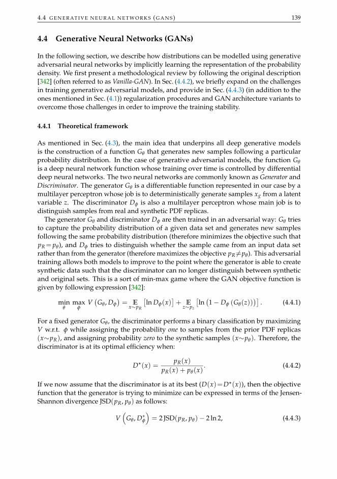
4.4 G E N E R AT I V E N E U R A L N E T W O R K S ( G A N S ) 139

4.4 Generative Neural Networks (GANs)

In the following section, we describe how distributions can be modelled using generativeadversarial neural networks by implicitly learning the representation of the probabilitydensity. We first present a methodological review by following the original description[342] (often referred to as Vanilla-GAN). In Sec. (4.4.2), we briefly expand on the challengesin training generative adversarial models, and provide in Sec. (4.4.3) (in addition to theones mentioned in Sec. (4.1)) regularization procedures and GAN architecture variants toovercome those challenges in order to improve the training stability.

4.4.1 Theoretical framework

As mentioned in Sec. (4.3), the main idea that underpins all deep generative modelsis the construction of a function Gθ that generates new samples following a particularprobability distribution. In the case of generative adversarial models, the function Gθ

is a deep neural network function whose training over time is controlled by differentialdeep neural networks. The two neural networks are commonly known as Generator andDiscriminator. The generator Gθ is a differentiable function represented in our case by amultilayer perceptron whose job is to deterministically generate samples xg from a latentvariable z. The discriminator Dφ is also a multilayer perceptron whose main job is todistinguish samples from real and synthetic PDF replicas.

The generator Gθ and discriminator Dφ are then trained in an adversarial way: Gθ triesto capture the probability distribution of a given data set and generates new samplesfollowing the same probability distribution (therefore minimizes the objective such thatpR= pθ), and Dφ tries to distinguish whether the sample came from an input data setrather than from the generator (therefore maximizes the objective pR 6=pθ). This adversarialtraining allows both models to improve to the point where the generator is able to createsynthetic data such that the discriminator can no longer distinguish between syntheticand original sets. This is a sort of min-max game where the GAN objective function isgiven by following expression [342]:

minθ

maxφ

V(Gθ , Dφ

)= E

x∼pR

[ln Dφ(x)

]+ E

z∼pz

[ln(1− Dφ (Gθ(z))

)]. (4.4.1)

For a fixed generator Gθ , the discriminator performs a binary classification by maximizingV w.r.t. φ while assigning the probability one to samples from the prior PDF replicas(x∼pR), and assigning probability zero to the synthetic samples (x∼pθ). Therefore, thediscriminator is at its optimal efficiency when:

D?(x) =pR(x)

pR(x) + pθ(x). (4.4.2)

If we now assume that the discriminator is at its best (D(x)=D?(x)), then the objectivefunction that the generator is trying to minimize can be expressed in terms of the Jensen-Shannon divergence JSD(pR, pθ) as follows:

V(

Gθ , D∗φ)= 2 JSD(pR, pθ)− 2 ln 2, (4.4.3)


x ∼ pR

z Gθ(z)xg ∼ pθ

Dφ(x)

Real

Fake

Figure 27 Diagrammatic structure of a generative adversarial neural network. Both neuralnetworks are represented in terms of deep convolutional neural networks (DCNNs). Thediscriminator is expressed by Dφ while the generator is expressed by Gθ . Both the trueinput data and the generated samples are fed into the discriminator which evaluateswhether or not the generated samples are similar to the true data.

where the Jensen-Shannon divergence satisfies all the properties of the Kullback-Leiblerdivergence and has the additional constraint that JSD(pR, pθ)=JSD(pθ , pR). We then seefrom Eqs. (4.4.1-4.4.3) that the best objective value we can achieve with optimal generatorand discriminator is (−2 ln 2).

The generator and discriminator are generally trained in the following way: the gener-ator generates a batch of synthetic samples that along with the samples from the inputdata sets are provided to the discriminator 1 (see Algorithm 1). Algorithm 1 is a typicalformulation of a generative-based adversarial strategy. The adversarial training of boththe discriminator and generator neural networks are described in Fig. 27. The traininggoes as follows. On the one hand, the generator takes as input a vector of random noisesand outputs fake data which then get fed into the discriminator. During the training of theGenerator, it is important that the discriminator is freezed, otherwise equilibrium mightnever be reached. On the other hand, the discriminator model takes as input both the trueand fake data. The model then outputs predictions as to whether the samples are realwith labels ones or fake with labels zeros. However, as we will discuss in the next section,working with such an implementation in practice is very challenging and often leads topoor results.

4.4.2 Challenges in training GANs

Training generative adversarial models can be very challenging due to the lack of stoppingcriteria that estimates when exactly GANs have finished training. Therefore, there isno guarantee that the equilibrium is reached. In addition, GANs have common failure

1 It is important that during the training of the generator, the discriminator is not trained. As it will be explainedlater, having an over-optimized discriminator leads to instabilities.

4.4 G E N E R AT I V E N E U R A L N E T W O R K S ( G A N S ) 141

Algorithm 1: Algorithm describing the stochastic gradient descent training of astandard generative adversarial networks [342].

for epochs 1, · · · , N dofor Discriminator steps 1, · · · , k do

- Sample minibatch of size m from the real sample: {x(1)r , · · · , x(m)r }

- Sample minibatch of size m from the latent space: {z(1), · · · , z(m)}- Perform gradient ascent on discriminator:

∇φV(Gθ , Dφ

)=

1m∇φ

m

∑i=1

ln Dφ

(x(i)r

)

+1m∇φ

m

∑i=1

ln(

1− Dφ

(Gθ

(z(i))))

endfor Generator steps 1, · · · , ` do

- Sample minibatch of size m from the latent space: {z(1), · · · , z(m)}- Perform gradient descent on generator:

∇θV(Gθ , Dφ

)=

1m∇θ

m

∑i=1

ln(

1− Dφ

(Gθ

(z(i))))

endend


modes due to inappropriate choices of network architecture, loss function or optimizationalgorithm. Several solutions have been proposed to address these issues which is still atopic subject to active research. For a review, we refer the reader to Refs. [343–345]. Inthis section, we briefly describe these challenges before providing some solutions in thenext section. The most encountered limitations of GANs in our case are: non-convergence,vanishing gradients, and mode collapse.

It is often the case that during optimization, the losses of generator and discriminatorcontinue to oscillate without converging to a clear stopping value. Although the existenceof an equilibrium (Nash Equilibrium) has been proved in the original GAN paper [342], thereis no guarantee that such an equilibrium will be reached in practice. This is mainly due tothe fact that the generator and discriminator are modelled in terms of neural networks,thus restricting the optimization procedures to the parameter space of the networks ratherthan learning directly from the probability distributions [344]. On the other hand, thisnon-convergence could happen even if the model has ventured near the equilibriumpoint. In this case, when the generated samples are far from the target distribution, thediscriminator pushes the generator towards the true data distribution while at the sametime increasing its slope. When the generated samples approaches the target distribution,the discriminator’s slope is the highest, pushing away the generator from the true datadistribution [346]. As a result, depending on the stopping criteria, the GAN optimizationmight not necessarily converge to a Nash equilibrium [342] in which the performance ofthe discriminator and generator cannot be improved further (i.e. optimal conditions). Insuch a scenario, the generated samples are just collections of random noise.

The vanishing gradients occur when the discriminator is over-optimized and does notprovide enough information to the generator to make substantial progress [343]. Duringbackpropagation, the gradient of the generator flows backward from the last layer to thefirst, getting smaller at each iteration. This raises some complications since, in practice, theobjective function of a discriminator close to optimal is not given by 2 JSD(pR, pθ)−2 ln 2as stated in Eq. (4.4.3), but rather close to zero. This then pushes the loss function to zero,providing little or no feedback to the generator. In such a case, the gradient does notchange the values of the weights in the initial layers, altering the training of the subsequentlayers.

Finally, the mode collapse occurs when the generator outputs samples of low diver-sity [347], i.e, the generator maps multiple distinct input to the same output. This is thecase where the generated samples from the GAN capture only a few of the modes of theinput data set. Mode collapse is a common pathology to all generative adversarial modelsas the cause is deeply rooted in the concept of GANs.

The challenges mentioned above contribute to the instabilities that arise in training GANmodels. What often complicates the situation is that these obstacles are linked with eachother and one might require a procedure that tackles all of them at the same time. As wewill briefly describe in the next section, there exist various regularization techniques, somespecific to the problem in question, that could influence the stability during the training.

4.4.3 Training stability & Regularization

Apart from the regularization procedures introduced in Sec. (4.1), there exists alternativeprocedures and techniques more suitable for generative adversarial models that can

4.5 S U M M A RY 143

alleviate the challenges described in Sec. (4.4.2). Whilst some of the procedures can beimposed on already defined GAN architecture, some are defined in terms of differentmodel variants. Here, we just list some of the most used and widespread techniques.

- Gradient Penalty:

One of the first line of defence against instabilities in training GANs is a techniqueknown as gradient penalty. This consists in imposing a penalty on the gradient of thediscriminator Dφ(x) in order to enhance its sensitivity in the regions Dφ(x)→ 0 andDφ(x)→ 1. The gradient penalty is applied to the logit of Dφ(x) as follows

Dφ(x) = ln(

Dφ(x)1− Dφ(x)

)−→ ∇Dφ(x) =

∇Dφ(x)Dφ(x)

(1− Dφ(x)

) . (4.4.4)

The penalty on the discriminator is applied in the regions where the predictionsare wrong, i.e. the discriminator assigning labels zero to true data, or converselyassigning labels one to fake data. The gradient penalty loss is therefore defined by

LGP = Ex∼pR

[(1− Dφ(x)

)2 |∇Dφ(x)|2]+ E

z∼pz

[Dφ (Gθ(z))

2 |∇Dφ(x)|2]

. (4.4.5)

In the case where the discriminator is perfectly well-trained the prefactors(1−Dφ(x)

)

and D2φ(x) vanish. The gradient penalty loss given in Eq. (4.4.5) can then be added to

the discriminator’s loss function LD=LD+λLGP with λ a properly chosen variable.

- Architecture variants:

In order to alleviate the challenges associated with the training of GANs, variousmodifications on the architecture (including loss function) have been proposed. Forinstance, it has been studied in Ref. [348, 349] that the generative capabilities of theGenerator is inherently bounded by the size of the discriminator’s architecture. Thishas motivated the use of large discriminator networks. On the other hand, the useof overparametrized discriminator may saturates the generator and hence ruin thetraining. However, this can be easily circumvented by restricting the weight updatesof the discriminator using for example the gradient penalty described above. Theseeventually led to the use of deep convolutional neural network to represent both thediscriminator and generator’s. There exists thus far various GAN variants, examplesare DCGAN [350, 351], INFOGAN [352], BIGGAN [353], et cetera. For the study ofPDFs, that will be presented in the next Chapter, we use a variant called WGAN [354].

- Hyperparameter Optimization:

One of the most robust ways to come up with stable networks that do not sufferfrom the issues mentioned before is the hyperparameter tuning in which a space ofparameter is scanned in order to find the optimal values given the metrics of interest.The choice of model (or variants) could even be regarded as a hyperparameter.Details on such a procedure are described in the next Chapter.

4.5 Summary

In this chapter, we reviewed the fundamentals of deep learning, explaining in details thevarious pieces that enter into the training of a deep neural network. We then provided a


brief description of what deep generative models are and how efficient they are in termsof modelling posterior distributions. In particular, we focused on generative adversarialneural networks, which differ from the other families of generative models in that GANsare likelihood-free. The challenges related to GANs were then discussed in details, as wellas the standard regularization procedures used to tackle them. Two possible applicationsof the GANs to parton densities are presented in the next chapter.

145

5

E F F I C I E N T C O M P R E S S I O N O F P D F S E T S U S I N G G A N S

It has been strongly emphasized in Chapter 1 that Parton Distribution Functions (PDFs) arecrucial ingredients for all predictions of physical observables that are of interest at hadroncolliders such as LHC, and efforts to make their determination accurate with smalleruncertainties have become increasingly relevant. In current phenomenology studies, apartfrom the theoretical uncertainties arising from missing higher-order corrections, they areone of the dominant sources of uncertainty in precision measurement. A striking exampleof such a limitation is the role that PDFs play in the extraction of the Higgs coupling fromdata [132]. It is therefore clear that for the sake of doing precision physics (an importantpath toward a deep understanding of the physics beyond the Standard Model), PDFs needto be accurate at a percent-level [4]. The road toward reaching such an accuracy manifestsat two distinct levels: (i) the determination of the PDFs through a fitting procedure, and(ii) the a posteriori treatment of the fitted results such as the reduction of the numberof Monte Carlo (MC) replicas (or number of eigenvectors in the case of Hessian PDFs).Recently, spectacular advancement has been seen at the level of the PDF determinationthanks to the inclusion of new (LHC) datasets and more importantly to the improvementin methodology, see Ref. [4] for ample details. In the following chapter, what we areinterested is the latter, specifically the compression of a Monte Carlo PDF replicas into asmaller set that replicates all the statistical properties of the starting PDF set (henceforthreferred to as prior).

Originally, the compression of Monte Carlo PDFs has been introduced in the contextof Combined PDF Sets. The idea consists in combining various PDF sets determinedby different PDF fitter groups that implement different methodologies. As mentionedbefore, to the present date, there exists various PDF fitter groups that implement differentmethodology and provide different estimation of the PDF errors [34–68, 68–73, 355, 356].As a consequence, even when benchmarking the different methodologies with the sameinput datasets, it has been shown that the resulting PDF sets still differ with a reasonableagreement [357]. Therefore, from the practical point of view, it seems reasonable to combinethe different PDF sets and evaluate the combined uncertainty in order to obtain estimatesof the PDF error that take into account the various methodologies.

Apart from its relevance for the combination of Monte Carlo PDF sets, the compressionmethodology is also useful for native Monte Carlo PDF. In the NNPDF fitting methodol-ogy where the PDFs are represented in terms of Monte Carlo replicas, a large number ofsuch replicas are required in order to give an accurate representation of the underlyingprobability distribution. Indeed, there has been considerable evidence that one mightrequire O(103) (or even O(104)) Monte Carlo replicas in order to converge to the asymp-totic result [358, 359]. Putting aside the practical limits that arise with the fitting of such

146 E F F I C I E N T C O M P R E S S I O N O F P D F S E T S U S I N G G A N S

a large ensemble of Monte Carlo replicas, dealing with a large PDF set when producingphenomenological studies or Monte Carlo simulations is not ideal. In order to circumventsuch issues, one could compress down the large sample of Monte Carlo replicas into asmaller set. However, when going from O(103) to say O(100), one has to make sure thatall the various statistical properties such as correlations between pairs of flavours arepreserved. This is where the compression approach comes into play as a mean to selecta subset of Monte Carlo replicas that provides an accurate representation of the priordistribution.

A compression methodology has been introduced in Ref. [358]. The basic conceptualidea of the compression lies on the search of a subset of replicas that reproduces best thestatistical features of the original Monte Carlo PDF set. It has been shown at the PDFlevel using NNPDF3.0 sets that a compressed set with Nc=100 replicas is reasonablyequivalent to a prior with Np=1000 replicas. We would like to propose a new compressionstrategy [360] that aims at providing a compressed set with an even smaller number ofreplicas when compared to the standard approach of Ref. [358], while providing a similarrepresentation of the original probability distribution. The framework we would liketo propose is based on the generative adversarial neural networks that was introducedin Sec. (4.4). The idea is to enhanced the statistics of a given input Monte Carlo PDF setby generating what we call synthetic replicas. These synthetic replicas are new replicasgenerated from the GANs and to some extent follow the same probability distribution asthe prior. The motivation behind this is based on the following observation: large samplesof Monte Carlo replicas contains fluctuations that average out to the an asymptotic limit;in the standard compression approach, the is idea is just to select samples that present lessfluctuations and contain the bulk of the statistical information present in the prior. Thissuggests that it should be possible to generate samples that contain less fluctuations andonce combined with the samples from the prior can lead to a more efficient compressedrepresentations of the full result.

This chapter is organized as follows. In Sec. (5.1), we review the mathematical frameworkof the compression methodology while at the same time introducing a new implemen-tation that is faster and most importantly can incorporate the GANs framework. TheGANPDFS framework is introduced in Sec. (5.2.1) in which we present the GAN architec-ture used in our implementation. We also comment on some regularization proceduresthat are specific to our problem in order to circumvent the issues related to the trainingstability described in Sec. (4.4.2). The concept of hyperparameter optimization is thenintroduced in order to fit the methodology by scanning the hyperparameter space. Theefficiency of the new framework is then assessed in Sec. (5.3) by comparing it against thestandard approach based on some statistical estimators. In Sec. (5.4), we further validateour methodology by producing phenomenological results for LHC observables both at thetotal inclusive and differential levels. In Sec. (5.5), we give an outlook on the potential ofusing the GANPDFS framework to tackle the issue of the finite size effect by by-passingthe need of fitting Monte Carlo replicas of O(104), or even beyond. Finally, in Sec. (5.6),we discuss why the GAN-based compression might not be relevant for NNPDF4.0 PDFsets and why that can be interpreted as an indication of the robustness of the NNPDF4.0methodology.

5.1 C O M P R E S S I O N : M E T H O D O L O G I C A L R E V I E W 147

5.1 Compression: methodological review

Let us briefly review the compression methodology for Monte Carlo PDF sets introducedin Ref. [358]. The following closely follows the description provided in the aforementionedreference. One can summarizes the main idea behind the compression of (combined)Monte Carlo PDFs as finding a subset of the original PDF set such that the statisticaldistance between the original and the compressed is minimal. This ensures that the loss ofstatistical information is as low as possible. In this sense, the compression methodology hasto rely on two main ingredients: a proper definition of the distance metric that quantify thedistinguishability between the prior and the compressed distributions, and an appropriateminimization algorithm that explores the space of possible combinations of PDF replicasthat leads to such a minima.

It was originally proposed in Ref. [358] that a suitable figure of merit to measure thedifference between two parton distribution functions is the error functio

ERF =1

NEST∑k

1Nk

∑i

(Ck(xi)− Pk(xi)

Pk(xi)

)2

, (5.1.1)

where k runs over a set of statistical estimators with Nk the associated normalizationfactor, Pk(xi) is the value of the estimator k computed at a given point i in the x-gridfor the prior set, and Ck(xi) is the corresponding value of the same estimator but for thecompressed distribution. Finally, NEST denotes the total number of statistical estimatorsinvolved in the minimization. The scale dependence is not explicit shown in Eq. (5.1.1)since the scale at which the the PDFs are evaluated is the same for all estimators. As in theoriginal compression methodology, we include as statistical estimators lower moments(such as mean and standard deviation) and standardized moments (such as Skewness andKurtosis). In addition, in order to preserve higher-moments and PDF-induced correlations,which are crucial for phenomenology studies, we also include the Kolmogorov-Smirnovdistance and the correlation between multiple PDF flavours. For each statistical estimator,the normalization factor has to be defined properly as it compensates for the variousorders of magnitude in different regions of (x, Q)-space that is mainly apparent in highermoments. Here, we rewrite their definitions:

Lower and higher moments:

Since the statistical properties of a PDF is mainly dominated by lower moments, theyshould be reproduced with higher accuracy in the compressed set. Let us denoteby Pr

i (xj) and Cri (xj) respectively the prior and compressed sets of replicas r for

a flavour i at the j-th position in the x-grid. The expression of the central value,standard deviation, Skewness, and Kurtosis for the prior are defined as

PCVi (xj, Q0) =

1NR

NR

∑r=1

Pri (xj, Q0) (5.1.2)

PSTDi (xj, Q0) =

√√√√ 1NR − 1

NR

∑r=1

(Pr

i (xj, Q0)− PCVi (xj, Q0)

)2 (5.1.3)


PSKEi (xj, Q0) =

1NR

NR

∑r=1

(Pr


PSTDi (xj, Q0)

)3

(5.1.4)

PKURi (xj, Q0) =

1NR

NR

∑r=1

(Pr


PSTDi (xj, Q0)

)4

(5.1.5)

where Q0 denotes the initial scale at which the prior PDF set is computed and NRrepresents the total number of replicas. The expressions for the compressed set canbe computed analogously by replacing P with C and changing the total numberof replicas to size of the compressed set. Notice that in the summation the centralreplicas r=0 is not considered. From these definitions, one can therefore define theerror function for the moment estimators. For each estimator k, the error function isdefined as

ERFk =1

Nk

n f

∑i=−n f

Nx

∑j=1

(Ck

i (xj, Q0)− Pki (xj, Q0)

Pki (xj, Q0)

)2

(5.1.6)

for k = CV, STD, SKE, KUR. The number of active flavour is denoted by n f whilethe size of the x-grid is denoted by Nx. The above equation is only valid if thedenominator is non-zero, hence we only consider the case where Pk

i (xj, Q0) 6= 0.The normalization factor Nk for a statistical estimator k is defined as the lower 68%confidence-level of Nrd random selections. This can be expressed as

Nk =1

Nrd

Nrd

∑t=1

n f

∑i=−n f

Nx

∑j=1

(Rt,k

i (xj, Q0)− Pki (xj, Q0)

Pki (xj, Q0)

)2

68%

(5.1.7)

where Rti(xj, Q0) represent the t-th random selection extracted from the prior and

contains the same number of replicas as the expected compressed set. This ensuresthat the value of the error function ERFk for an estimator k is below 1.

Kolmogorov-Smirnov distance:

Since PDFs are continuous probability distributions, despite the fact that they areonly available as an interpolation on the grid of x-points, the Kolmogorov-Smirnovtest [361] (or its refinement, the Anderson-Darling test [362]) is a sensible estimator.In the context of PDF compression, the Kolmogorov-Smirnov distance is computedas follows [358]: for the prior set (resp. compressed), we count the number of replicasthat falls within a given region and then normalize by the total number of replicasin the prior (resp. compressed). As in the original compression, we consider sixdifferent regions which are defined in terms of the standard deviation

[−∞,−2PSTD

i (xj),−PSTDi (xj), 0, PSTD

i (xj), 2PSTDi (xj),+∞

]. (5.1.8)

The contribution to the error function from the Kolmogorov-Smirnov can thereforebe defined in the following way

ERFKS =1

Nk

6

∑z=1

n f

∑i=−n f

Nx

∑j=1

(Cz

i (xj, Q0)− Pzi (xj, Q0)

Pzi (xj, Q0)

)2

, (5.1.9)

5.1 C O M P R E S S I O N : M E T H O D O L O G I C A L R E V I E W 149

Input PDF withshape (Np, nf , xLHA)

Reduced setof replicas

Total ERF GA/CMA

Converges

Stop pyCompressor

No

Yes

Figure 28 Flowchart describing the methodology for the compression of Monte Carlo PDFreplicas. It takes as input a prior PDF set constructed as a grid in (NR, n f , x)-space andadditional parameters such as the size of the compressed set and the choice of minimizationalgorithm. The output is a Monte Carlo replicas with a reduced size that follows theLHAPDF [5] grid format.

with z running through the six regions defined in Eq. (5.1.8). The normalizationfactor is then defined as

NKS =1

Nrd

6

∑z=1

Nrd

∑t=1

n f

∑i=−n f

Nx

∑j=1

(Rt,z

i (xj, Q0)− Pzi (xj, Q0)

Pzi (xj, Q0)

)2

, (5.1.10)

where all the remaining symbols carry the same meaning as for the moments.

Correlations between PDFs:

As mentioned previously, it is important that the compressed set preserve PDF-induced correlations in physical cross sections. They play an important role inphenomenological studies. As a matter of fact, one of the main differences betweena fit with 100 and 1000 replicas is that correlations between pairs of flavours arereproduced more accurately in the latter. In order to define the error function for thecorrelation, we introduce the correlation matrixM whose elements are defined as

Mij =NR

NR − 1〈ij〉 − 〈i〉〈j〉

ΣiΣj. (5.1.11)

The brackets in the above equation are defined as follows

〈i〉 = 1NR

NR

∑r=1

f ri (xi, Q0), 〈ij〉 = 1

NR

NR

∑r=1

f ri (xi, Q0) f r

j (xj, Q0) (5.1.12)

where f ri (xi, Q0) denotes the replicas r from either the prior or compressed set with

flavour i and computed at the j-th position in the x-grid. The Σi represents the


10 85 160 235 310 385 460 535 610 685 760 835 910 985Size of Compressed Sets Nc

0

10

20

30

40

50T

ime

(mn

)Compressor

pyCompressor

Figure 29 Speed benchmark comparing the old and new compression codes using the GAas the minimizer. The prior set is a NNPDF3.1 set with Np=1000 replicas. On the y-axisis shown the time (in minutes) that it takes to perform a compression while the x-axisrepresents the various size of compressed sets. For the purpose of these benchmarks, theparameters entering the Genetic Algorithm (GA) are chosen to be exactly the same acrossboth implementations.

standard deviation and its expression is exactly similar to Eq. (5.1.3). We can nowdefine the contribution of the correlation to the error function as

ERFCR =1

NCR

(c− p

p

)2(5.1.13)

with the prior and compressed components respectively defined as

p = Tr(P · P−1

), c = Tr

(C · P−1

), (5.1.14)

where P and C respectively represent the correlation matrix of the prior and com-pressed set computed according to Eq. (5.1.11) and P−1 the inverse of P . Thenormalization factor NCR is computed analogously to the previous definitions, i.e.computed from a certain number of random selection.

Once the set of statistical estimators and the target size of the compressed set are defined,the compression algorithm can start the minimization procedure by searching for thecombination of replicas that leads to the minimal value of the total error function definedin Eq. (5.1.1). In order to select the replicas entering into the compressed set, variousminimization algorithms can be implemented. However, due to the discrete nature of thecompression problem, it is convenient to use minimization based on Evolution Algorithm(EA) [363, 364] such as the Covariance Matrix Adaptation (CMA) strategy [365, 366] or

5.2 C O M P R E S S I N G P D F S E T S W I T H G A N S 151

the Genetica Algorithm (GA) [367–369]. It is important to emphasize that no matter thechoice of minimization algorithm is, one can never run into the risk of overfitting since theabsolute minimum always exists. In Fig. 28, we show a diagrammatic representation ofthe compression workflow. It goes as follows: we first compute a grid of the prior PDF setfor all replicas, flavours, and all points of the x-grid; then we choose a random subset fromthe prior in order to compute the value of the total error function; this process is repeatedfor a certain number of iterations making sure that the minimizer selects a better sampleat every next iteration. The x-grid is constructed such that the points are distributed inthe region where experimental data are available. That is, one choose x to lie within the[10−5, 0.9

]-region such that the points are logarithmically spaced between

[10−5, 10−1]

and linearly spaced in the[10−1, 0.9

]-region.

The methodology described above was first implemented in a C++ code [358] andlater revised in Ref. [360, 370] using state-of-the-art python development. The new imple-mentation was required in order to accommodate for the generative models as will bediscussed in the next section. Here and henceforth, we referred to the new implementationas PYCOMPRESSOR. An important benefit of the new implementation is also the gain inperformance. Indeed, we observed that the new implementation is significantly faster ascompared to the old one. In order to quantify such a gain, we compress a Monte Carlo PDFset with Np = 1000 replicas into various sets with smaller sizes using the GA minimizer.The tests were run on a consumer-grade CPU1 with 16 GB of memory. The results arepresented in Fig. 29: on the x-axis are shown the various sizes of compressed sets whilethe required time for both compression codes to complete the same compression is shownon the y-axis. We can see that the new implementation is up to six times faster than theold one. One can also notice that the speed gain depends on the size of the compressedset. Not surprisingly, the difference between the two implementations increases as the thesize of the compressed set gets bigger. This is due to the fact that PYCOMPRESSOR takesadvantage of the multicore capabilities of modern computers2.

5.2 Compressing PDF sets with GANs

This section is devoted to the description of our generative adversarial model, henceforthreferred to as GANPDFS, and its incorporation into the compression methodology. Inparticular, we address the issue of instability when generating synthetic replicas. Sec. (4.4.2)introduced the general complexities of building a generative adversarial model in whichwe also discussed about various regularization procedures that can be used to alleviatesuch issues. Here, we specifically describe regularization procedures that are specific toour problem.

5.2.1 The GANPDFS methodology

Let us first restate again what we are trying to achieve. The problem we are concernedwith is the following: suppose that the prior Monte Carlo PDF replicas follow a probability

1 AMD Ryzen 5 2600 with 12 threads boosted at 3.4 GHz.2 Notice that the gain in speed due to the parallelization comes at the expense of a slightly higher memory usage.

Although this is a very minor issue, this can become significant if the both he sizes of the prior and compressedsets are very large.


Figure 30 Illustration of non-convergence (left) and mode collapse (right) when generatingMonte Carlo PDF replica. Here, we show the PDF for the d-quark. The priors are rep-resented by the green curves while the synthetic replicas are represented by the orangecurves. The two plots we generated using the vanilla implementation of the generativeneural network.

distribution pR, we would like to generate synthetic replicas following a probabilitydistribution pθ such that pθ is as close as possible to pR. One way to achieve this is bydefining a latent variable z with a fixed probability distribution pz. The latent variable zcan then be passed as an input to a function Gθ : z→ xg which is generally defined to be aneural network in order to generate samples that follow a probability pθ . By optimizingthe parameter θ, one can modify the distribution pθ to approach the target distribution pR.Here, we propose to model the function Gθ in terms of a generative neural network andassess the goodness of the output using a discriminative neural network, hence the idea ofgenerative adversarial neural networks (GANs).

The GANPDFS framework & Regularization

By adopting the standard variation (Vanilla) GANs introduced in the previous section, itis very likely that one ends up with the problem of instabilities described in Sec. (4.4.2).For the generation of synthetic replicas, the most likely scenarios are the non-convergenceand mode collapse (see Fig. 30 for illustrations). Whilst the non-converging result mustdefinitely be disregarded, the mode-collapse could still provide replicas that can be usedfor compression. Ideally, one would like the samples of synthetic replicas to reproduce theoverall distribution of the prior, not only some part of it. It was argued in Sec. (4.4.2) thatone of the main causes leading to unstable optimization during the training of a GAN isthe low dimensional support of generated and target distribution. This means that thegenerator can only generate scarce samples from the input latent variable z and does notallow for any improvement at all. As suggested in Ref. [346], this could be overcome byproviding to the latent variable z additional information. That is, one needs to supplythe input latent variable with some relevant features from the real sample. In our case,this could be done by taking a linear combination of the input PDF replicas, adding on


top of it Gaussian noises, and using it as the input latent variable. This has been provedto improve significantly the stability of the GAN training and addresses the problem ofnon-convergence.

On the other hand, it was also discussed in Sec. (4.4.2) based on Refs. [371, 372] that theobjective function that the standard (original) GAN minimizes is not continuous w.r.t thegenerator’s parameters. One can immediately see the shortcoming of this. Indeed, thiscan lead to both vanishing gradients and mode collapse. Such shortcomings were alreadyperceived in the original GAN paper [342] where it was shown that the Jensen-Shannondivergence under idealized conditions contributes to oscillating behaviours. Severalresearch papers have devoted to finding a suitable objective function in order to circumventthese particular problems (See Refs. [343, 344, 346] for a review). In our implementation,we resort to a loss function that was briefly introduced in Sec. (4.4.2): the Wassersteinor Earth’s Mover (EM) distance. This objective function was subsequently implementedin Wasserstein GAN (WGAN) [354, 373, 374] as application to image generation and hasproved to not only yield more stability but also more variety in the generated sample. TheEM loss function is defined as follows

minθ

maxφ

V = Ex∼pR

[Dφ(x)

]− E

x∼pθ

[Dφ(xg)

], (5.2.1)

where we recall that xg = Gθ(z) with z following a probability distribution pz. TheEM is effective in solving vanishing gradients and model collapse as it is continuouslydifferentiable w.r.t the generator and discriminator’s parameters. That is, GAN-basedWasserstein models result in a discriminator function whose gradient w.r.t its inputs isbetter behaved than in the standard GAN approach. This means that the discriminatorcan be trained until optimality without worrying about vanishing gradients.

Despite the fact that the Wasserstein distance measure yields non-zero gradients every-where for the discriminator, the resulting GAN architecture can still be unstable whenthe gradients of the loss function are large. This can straightforwardly be addressed byclipping the weights of the discriminator to lie within a compact space defined by [−c, c]where c is just some finite not-so-large number. Based on all of this, the default GANPDFS

architecture is a modified version of a WGAN and is described in Algorithm 2. If the needsarise, the GANPDFS codes allow the users to straightforwardly define a new architecturefrom an input file.

The hyperparameter optimization

We have just described a possible architecture for our generative models that can alleviatethe issues related to stability during the training, however, there is still some arbitrarinessin choosing the parameter that each neural network (generator or discriminator) can take.Indeed, one of the main factors that influence the training of a GAN is the architecture ofthe neural networks. The choice of (hyper) parameters could scale up significantly theGAN’s performance. However, coming up with values for hyperparameters such as thesize of the network or the number of nodes in a given layer is particularly challenging as theparameter space is very large and obviously trying blindly various hyperparameters doesnot appear to be a suitable solution. A heuristic approach to tackle this problem–whichis widely regarded as the best option within the machine learning community–is knownas hyperparameter scan or hyperparameter optimization. This approach consists in searching


Algorithm 2: Default stochastic gradient descent training algorithm imple-mented in GANPDFS for the generation of synthetic replicas.

for epochs 1, · · · , N dofor discriminator steps 1, · · · , k do

- Sample minibatch of size m from the original input sample:{x(1)r , · · · , x(m)

r }- Sample minibatch of size m from the custom latent space: {z(1), · · · , z(m)}- Perform gradient ascent on discriminator:

∇φV(Gθ , Dφ

)=

1m∇φ

m

∑i=1

(Dφ

(x(i)r

)− Dφ

(x(i)g

))

- φ = φ + RMSProp(φ,∇φV)- Clip weights within [−c, c]

endfor generator steps 1, · · · , l do

- Sample minibatch of size m from the custom latent space: {z(1), · · · , z(m)}- Perform gradient descent on generator:

∇θV(Gθ , Dφ

)=

1m∇θ

m

∑i=1

Dφ

(x(i)g

)

- θ = θ − RMSProp(θ,∇θV)end

end


Input LatentSpace z

Input PDF(Np, nf , xLHA)

xr ∼ pr

GeneratorGθ(z)

Synthetic Repl.(Ns, nf , xGAN)

xg ∼ pθ

DiscriminatorDφ(xS , xR)

(Ns, nf , xGAN)

GAN

Enhanced PDF(Np + Ns, nf , xLHA)

Interpolation

Figure 31 Flowchart describing the GANPDFS framework. The discriminator receives asinput the prior PDF set computed as a grid in (Np, n f , xLHA)-points while the generatorreceives as input the latent variable constructed as Gaussian noise of linear combination ofthe prior set. In addition to the real sample, the output of the generator also goes throughthe discriminator. The simoultaneous training of both neural networks goes on until acertain number of epochs is reached. The final output is an enhanced PDF following theLHAPDF grid format.

the best set of hyperparameters through an iterative search of the parameter space. Inour implementation, we rely on the Tree-structured Parzen Estimator (TPE) [375] as anoptimization algorithm. The TPE consists in building a probability model of the objectivefunction and use it to select the most promising hyperparameters to evaluate the trueobjective function. Such a method outperforms by a significant amount any random search.The main challenge in performing such a hyperparameter optimization, however, is thedefinition of a figure of merit to hyper-optimize on. Indeed, there is no established figureof merit for generative models that can be used to assess the faithfulness of the generatedsamples. One possibility is to use one of the statistical estimators described in Sec. (5.1),but in doing so we restrict ourselves to only a particular feature of the distribution. In ourgenerative model, we decide to use the Frechet Inception Distance (FID) [376] as the figure


of merit to hyperoptimize on. For a target distribution with mean µr and covariance Σrand a synthetic distribution with mean µs and covariance Σs, the FID is defined as:

FID =1

2n f + 1

n f

∑i=−n f

∥∥∥µ(i)r − µ

(i)s

∥∥∥2+ Tr

(Σ(i)

r + Σ(i)s − 2

√Σ(i)

r Σ(i)s

)(5.2.2)

where the index i refers to the parton flavours. This suggests that the smaller the valueof the FID is, the closer the generated samples are to the target distributions. For theimplementation of the TPE hyperoptimization procedure in our GAN framework, we relyon a third party library called HYPEROPT [377].

We can now proceed to the description of our GANPDFS workflow. In Fig. 31 weshow a diagrammatic summary of the training. Let us first mention that our implemen-tation is based on the machine learning framework TENSORFLOW [378] using KERAS asa backend [379, 380]. Focusing now on Fig. 31, we see that in order to train, the GAN-PDFS receives as input a grid of shape (Np, n f , xLHA) where Np represents the numberof input replicas and xLHA denotes the size of the x-grid which corresponds exactly tothe internal LHAPDF-grid. The input grid is then passed to the discriminator and willbe used to assess the generated replicas from the generator. Separately, the generatortakes as input the latent variable z and outputs a grid of shape (Ns, n f , xGAN). Notice thatxGAN does not have to be the same as xLHA. This is because it has been observed that thegenerator trains better when provided with a large size of x-grid. In such a case, an inter-polation is required in order to produce a LHAPDF-like grid. By default, xGAN is a gridof Nx=500 points logarithmically spaced in the small-x region

[10−9, 10−1] and linearly

space in the large-x region[10−1, 1

]. The output of the GANPDFS is then a LHAPDF grid

with (Np + Ns)-replicas at a starting scale Q0=1.65 GeV which can then be evolved usingAPFEL [381]. Notice that physical constraints such as positivity of the PDFs or sum rulesare not enforced but rather inferred from the underlying distribution.

5.2.2 The GAN-enhanced compression methodology

Having separately introduced the concepts of compression and generative adversarialmodel for Monte Carlo PDF replicas, we now provide a description on how these twocomponents can be incorporated into one single framework. In Fig. 32, we present aschematic diagram describing how the two frameworks are interfaced together. Theworkflow goes as follows: the input PDF grid is computed for a given Monte Carlo PDFset containing Np replicas at fixed Q0 (which by default is set to Q0=1.65 GeV) and atsome value of the Bjorken x. If enhancing the statistics of the prior with the GAN is notrequired, then the reduction strategy follows the standard compression methodologyintroduced in Sec. (5.1). If, on the other hand, the GAN-enhancement is required, theGANPDFS is used to to generate Ns synthetic replicas. The synthetic replicas combinedwith the prior, which henceforth we call enhanced set, has now a total size NE=Np + Ns.As mentioned before, since the x-grid of the output of the GAN does not necessarily haveto be the same as for the prior, an interpolation might be required in order to combine thetwo. The enhanced (or combined) set is then passed to the PYCOMPRESSOR . It is crucialto emphasize that in the context of GAN-enhanced compression, the samples of replicasthat will end up in the compressed set are drawn from the enhanced set rather than from


Input PDF withshape (Np, nf , xLHA)

Enhance

Np + Ns

replicasNp

replicas

Reduced setof replicas

Total ERF GA/CMA

Converges

Stop pyCompressor

GAN

Yes No

No

Yes

Figure 32 Flowchart describing the combined GANPDFS-PYCOMPRESSOR framework. Theworkflow starts with the computation of the prior MC PDF as a grid of (Np, n f , xLHA). IfGAN-enhanced is required, the prior replicas are supplemented with synthetic replicas.If not, the compression follows the standard methodology. The output is always a com-pressed set containing smaller numbers of replicas.

the prior only. However, since the main goal is still to construct a compressed set thatreproduces the probability distribution of the prior, the minimization has to be performedw.r.t the input Monte Carlo PDF replicas. In this sense, the expression of the total errorfunction in Eq. (5.1.1) has to be modified such that the value of the estimator Ck for thecompressed set has to be computed using samples from the enhanced distribution. Westress that the expression of the normalization factors does not change, i.e. the randomsets of replicas have to be extracted from the prior.

Adiabatic minimization

Performing a compression from an enhanced set can be very challenging due to thelarge number of replicas to be considered. Indeed, the factorial growth of the numberof replicas can probe the limit of the minimization algorithm and may potentially spoilthe minimization procedure. In other words, the vast nature of the space of replicathat could be explored increases the odd of the compression to be stuck in some localminima. However, if results from the standard compression are already provided, thecompression code provides a more efficient compression procedure from the enhanced setwith the means of an adiabatic minimization. The adiabatic minimization for the enhancedcompression consists on taking as a starting point the space of replicas where the best fromthe standard compression was generated and start from there. Such a minimization not


Glorot Uniform Random UniformDisc. Kernel Initializer

1.0

1.5

2.0

2.5

3.0

3.5

FID

1000 1500 2000Nb. Epochs

FID

Glorot Uniform Random UniformGen. Kernel Initializer

FID

2 3 4Disc. Steps

FID

1 2 3Gen. Steps

FID

Figure 33 Graphical representation of an hyperparameter scan for a few selected param-eters. The results were produced with a certain number of trial searches using the TPEalgorithm. On the y-axis is represented the different values of the FID while the varioushyperparameters are represented on the x-axis. The violin plots represent the behaviourof the training for a given hyperparameter and violins with denser tails are consideredbetter choices due to their stability.

only yields faster convergence but also prevent the minimization algorithm to be trappedin some local minimum in case the generated replicas from the GAN contains fluctuations.

Hyperoptimized architecture

In this section, we present the GANPDFS architecture that has come out as the result ofan hyperparameter optimization. The setup in which we performed the hyperparameteroptimization is as follows: we considered as a prior a Monte Carlo PDF replicas withNp=1000 replicas fitted using the NNPDF3.1 methodology [49]. We then use the GAN-PDFS to generate Ns=2000 synthetic replicas for a total of NE=3000 enhanced replicas.This procedure is repeated for a certain number of iteration through the hyperparameterscan by minimizing the FID. In Fig. 33, we plot an example of a hyperparameter scan inwhich a few selected parameters are shown. These are results after performing a certainnumber of trials. For each hyperparameter, the values of the FID are plotted as a function ofthe different parameters. For the initialization of the discriminator’s weights, for instance,there are two choices, namely the Glorot Uniform and the Random Uniform. The values

5.3 E F F I C I E N C Y O F T H E N E W G A N - E N H A N C E D C O M P R E S S I O N 159

Generator DiscriminatorNetwork depth 3 2kernel initializer glorot uniform glorot uniformweight clipping - 0.01

optimizer None RMSpropactivation leakyrelu leakyrelu

steps 1 4batch size 70%

number of epochs 1000

Table 2 Parameters on which the hyper-parameter scan was performed are shown in thefirst column. The resulting best values are shown for both the generator and discriminatorin the second and third column respectively.

of the FIDs are represented by the gray points and the violin shapes represent the densityof gray points within a particular region. In this sense, the violin plots represent a visualillustration of how a given parameter behave during the training. That is, violins withdenser tails are considered better choices as they yield more stable training. For instance,we can see that 1000 epochs lead to a slightly more stable results as opposed to 1500 or2000. For a complete summary, the list of hyperparameters with the corresponding valuesare shown in Table 2.

5.3 Efficiency of the new GAN-enhanced compression

In the following sections, we quantify the performance of the GAN-enhanced frameworkover the standard approach by subjecting both methodologies on various statistical tests.As for the hyperparameter scan, all the analyses presented here were produced with the fol-lowing setup: the prior contains Np=1000 replicas fitted with the NNPDF3.1 methodologywhich then gets enhanced with the GANPDFS framework in order to generate NE=3000replicas (i.e. Ns=2000 replicas). The compression of the native prior and GAN-enhancedreplicas are both handled by the PYCOMPRESSOR.

5.3.1 Validation of the GAN methodology

First, we would like to see, for a given compression from the enhanced set, how manyreplicas are selected from the synthetic samples. In order to do so, we perform two typesof compression: one with the GAN-enhanced methodology and one with the standardapproach. In Fig. 34, we show the disparity between the standard and GAN-enhancedcompressed sets, i.e. the number of replicas that are present in the GAN-enhanced com-pressed sets (including synthetic replicas) but not in the standard sets. The results areshown for different sizes of the compressed sets. The green histograms represent thenumber of replicas that are not present in the final set of the standard approach but presentin the GAN-enhanced compressed sets. The orange histograms represent the numberof synthetic replicas out of that disparity. We can see that for smaller compressed sizes(smaller than Nc=200), the percentage of synthetic replicas that compose the compressed


30 40 50 60 70 80 90 100 200 300 400 500 600 700 800 900size of compressed set

0

10

20

30

40

50

60

70nu

mbe

r of r

eplic

as

1214

9

19

14

2624

42 4238 39

7276

55

61

44

97 7

11 10

1816

22 2325 25

4844 45 45

33

Disparity rates between Standard and Enhancedextra-replicassynthetic replicas

Figure 34 Histograms representing the number of disjoint replicas that are present in theGAN-enhanced compressed set but not in the standard. That is, the green histograms areconstructed by counting the number of replicas from the GAN-enhanced compression thatare not seen after the standard compression. Out of these numbers, the green histogramsrepresent the number of replicas that are coming from the synthetic replicas. The resultsare shown as a function of the size of the compressed set.

set exceeds 10% and this percentage decreases as the size of the compressed set increases.This is explained by the fact that as the size of the targeted compressed set approaches thesize of the prior Monte Carlo PDF replicas, the probability distribution of the reduced realsamples get closer to the prior such that fewer synthetics are required.

Now, we turn to the validation of the GAN-enhanced compression methodology by firstlooking at the PDF central values and luminosities. In Fig. 35 we show the absolute centralvalues resulting from the GAN-enhanced compression at an energy scale Q=1.65 GeV. Theresults are shown for various PDF flavours (g, s, d, s) and for different size of compressedsets (Nc=50, 70, 100). The results are normalized to the the central value of the prior MonteCarlo PDF replicas. In order to qualitatively assess whether or not compressed sets withsize Nc=50, 70, 100 are good representations of the prior probability distribution, we alsoplot the 68% and 1-sigma bands. We see that, for all the three sets, the PDF uncertaintiesare much larger than the fluctuations of the central values, indicating that a compressedset with Nc=50 captures the main statistical properties of the prior. In Fig. 36, we plotsthe luminosities for the g-g, d-u, and d-u combinations as a function of the invariant massof the parton pair Mx for two different sizes of compressed sets, namely Nc=50, 70, 100.As previously, the hatched bands represent the 68% confidence interval while the the 1-sigma bands are represented by the dashed lines. The compressed sets Nc=50, 70 slightlydeviate from the underlying probability distributions at lower values of Mx in whichPDFs are known to be non-Gaussian. However, one can notice that the deviations are


10 5 10 4 10 3 10 2 10 1 100

x

0.7

0.8

0.9

1.0

1.1

1.2

1.3Ra

tio to

Prio

rg at 1.6 GeV

Prior (68 c.l.+1 )GAN-enhanced Nc = 50GAN-enhanced Nc = 70GAN-enhanced Nc = 100Standard Nc = 100

10 5 10 4 10 3 10 2 10 1 100

x

0.7

0.8

0.9

1.0

1.1

1.2

1.3

Ratio

to P

rior

s at 1.6 GeVPrior (68 c.l.+1 )GAN-enhanced Nc = 50GAN-enhanced Nc = 70GAN-enhanced Nc = 100Standard Nc = 100

10 5 10 4 10 3 10 2 10 1 100

x

0.7

0.8

0.9

1.0

1.1

1.2

1.3

Ratio

to P

rior

d at 1.6 GeV


10 5 10 4 10 3 10 2 10 1 100

x

0.7

0.8

0.9

1.0

1.1

1.2

1.3

Ratio

to P

rior

d at 1.6 GeV


10 5 10 4 10 3 10 2 10 1 100

x

0.7

0.8

0.9

1.0

1.1

1.2

1.3

Ratio

to P

rior

u at 1.6 GeV


10 5 10 4 10 3 10 2 10 1 100

x

0.7

0.8

0.9

1.0

1.1

1.2

1.3

Ratio

to P

rior

u at 1.6 GeV


Figure 35 Comparison of the PDF central values resulting from the compression usingthe GAN-enhanced methodology for different values of Nc=50, 70, 100 and different PDFflavours (g, s, d, u, d). Results are normalized to the central value of the prior set. The 68%confidence interval is represented by the green hatched band whole the 1-sigma band isrepresented by the dashed green lines. The PDFs are computed at Q=1.65 GeV. Plotsproduced using REPORTENGINE-based VALIDPHYS [6] suite.

very small compared to the uncertainty bands. For Nc=100, we see very good agreementbetween the prior and the GAN-enhanced compressed set. These plots further strengthenthe observations made at the level of central values. The above results confirm thatcompressed sets constructed from the GANPDFS-PYCOMPRESSOR methodology fullypreserve the PDF central values and luminosities between pairs of PDFs. In particular, we


101 102 103

mX (GeV)

0.85

0.90

0.95

1.00

1.05

1.10

1.15Ra

tio to

Prio

rgg luminosity

s = 13 TeV

Prior (68 c.l.+1 )Nc = 50 (68 c.l.+1 )

101 102 103

mX (GeV)

0.85

0.90

0.95

1.00

1.05

1.10

1.15

Ratio

to P

rior

du luminositys = 13 TeV

Prior (68 c.l.+1 )Nc = 50 (68 c.l.+1 )

101 102 103

mX (GeV)

0.85

0.90

0.95

1.00

1.05

1.10

1.15

Ratio

to P

rior

gg luminositys = 13 TeV

Prior (68 c.l.+1 )Nc = 70 (68 c.l.+1 )

101 102 103

mX (GeV)

0.85

0.90

0.95

1.00

1.05

1.10

1.15

Ratio

to P

rior


Prior (68 c.l.+1 )Nc = 70 (68 c.l.+1 )

101 102 103

mX (GeV)

0.85

0.90

0.95

1.00

1.05

1.10

1.15

Ratio

to P

rior

gg luminositys = 13 TeV

Prior (68 c.l.+1 )Nc = 100 (68 c.l.+1 )

101 102 103

mX (GeV)

0.85

0.90

0.95

1.00

1.05

1.10

1.15

Ratio

to P

rior


Prior (68 c.l.+1 )Nc = 100 (68 c.l.+1 )

Figure 36 Comparison of the PDF luminosities between the prior and the GAN-enhancedcompressed sets at LHC with

√s=13 TeV. The results are shown for different sizes of

compressed sets, namely (Nc=50, 70, 100) and for different PDF luminosities (g-g, d-u,and d-u). The hatched error bands and the region envelopped with the dashed linesrepresent the 68% confidence level and 1-sigma deviation respectively. Plots producedusing REPORTENGINE-based VALIDPHYS [6].

conclude that about Nc=50 replicas sufficient enough to reproduce the main statisticalproperties of a prior Monte Carlo PDF with Np=1000 replicas. Next, we quantify howefficient is the generative-based compression methodology compared to the standardapproach of Ref. [358].


5.3.2 Performance of the generative-based compressor

In order to qualitatively quantify the performance of the new generative-based compres-sion methodology, we evaluate the compressed sets resulting from the new and standardmethodologies on various statistical estimators. We consider the same settings as in theprevious sections in which the results of the GAN-enhanced compression are compared tothe results from the standard approach where the samples of replicas are selected directlyfrom the prior Monte Carlo PDF.

Let us start by comparing the two methodologies at the level of the error functions.In Fig. 37, for each compressed set, we show the contribution of each of the statisticalestimator (see in Sec. (5.1) for details) that contribute to the total value of the ERF usingthe standard (green) and GAN-enhanced (orange) approach as a function of the size of thecompressed set. Notice that the ERFs shown in the plot are non-normalized. This is indeedirrelevant when comparing the two methodologies since the normalizations are the samein both approaches. For reference, we also show the mean (purple) and median (lightblue) computed by taking the average ERF values from NR=1000 random selections. Toprovide an estimate of how representative of the prior distribution a random compressedset is, the confidence intervals (50%, 68%, 90%) computed from the random selections arealso shown as error bars of varying colours.

First of all, as expected, we see that as the size of the compressed set increases, theERF values of all the estimators tend to zero. The fact that the correlation present somefluctuations support our claim that as opposed to the lower and higher moments, cor-relations are difficult to preserve. On the other hand, it is clear that both compressionmethodologies outperform quite significantly any random selection of replicas. But inaddition, by comparing the results from the standard and GAN-enhanced approach, weobserve that the estimators for the GAN-enhanced compression, are in all cases except fora very few, below those of the standard compression. Indeed, it could happen that theerror function for a given estimator for the standard approach is lower than the GAN whilethe total value of the error function is still lower for the latter. Overall, this suggests thatthe GAN-enhanced approach will result in a total value of the ERF that is much smallerthan the one from the standard compression methodology.

In terms of efficiency, these results imply that the new generative-based methodologyoutperforms the standard compression approach by providing a more adequate represen-tation of the probability distribution of the prior thanks to the synthetic replicas. This isparticularly illustrated in Fig. 38 in which we plot in solid black line the total value of theerror function for the standard compression as a function of the size of the compressedset. The vertical dashed lines represent the size of the compressed set Nc=70, 90, 100while the horizontal solid lines represent the respective ERF values for the GAN-enhancedcompressed sets. The intersection between vertical dashed lines and horizontal solidlines being below the black line strongly indicate that the generative-based compressionoutperforms the standard approach. For instance, we see that Nc=70 from the enhancedcompressed set is equivalent to about Nc=110 from the standard approach, and Nc=90from the enhanced set provides slightly more statistics that Nc=150 from the standardcompression methodology.

In addition to the above checks, one can also verify that correlations between PDFsare well preserved after the compression. It is important to emphasize that one of the


90080070060050040030020010090807060504030

10 9

10 7

10 5

10 3

10 1

NC

ERF correlation

90080070060050040030020010090807060504030

101

102

103

NC

ERF kolmogorov_smirnov

90080070060050040030020010090807060504030

101

102

103

104

105

NC

ERF mean

90080070060050040030020010090807060504030

10 1

100

101

NC

ERF stdev

90080070060050040030020010090807060504030

103

104

105

106

NC

ERF skewness

90080070060050040030020010090807060504030

100

101

102

NC

ERF kurtosis

Random Mean (1k)Random Median (1k)StandardEnhanced

Random 50% c.l. (1k)Random 68% c.l. (1k)Random 90% c.l. (1k)

Figure 37 Comparison of the best ERF values for the compression of a Monte Carlo PDFset with Np=1000 replicas for various sizes of the compressed sets. For each compressedset, we show the contribution of the statistical estimators (see Sec. (5.1)) that contribute tothe total error function using the standard compression (green) and the GAN-enhancedcompression (orange) methodology. Notice that the ERFs on the plot are non-normalized.For illustration purposes, the mean (purple) and median (light blue) resulting from theaverage of NR=1000 random selections are shown. The resulting confidence intervalsfrom the random selections are represented by the blue (50%), green (68%), and red (90%)error bars.

main differences between a fit with 100 and 1000 Monte Carlo replicas is that correlationsare reproduced more accurately in the latter [358]. This is one of the main reasons whythe compression methodology is important. Here, we show that for the same size ofcompressed set, the resulting compression from the GAN-enhanced methodology also


60 80 100 120 140 160 180 200Size of Compressed Set

0.14

0.15

0.16

0.17

0.18

0.19

ERF

compressor vs. pyCompressor performanceStandard ERFsSynth. Nc=70Synth. Nc=90Synth. Nc=100

Figure 38 Comparison of the performance of the new generative-based compression algo-rithm (GANPDFS) and the previous methodology (standard). The normalized ERF valuesof the standard compression are plotted as a function of the size Nc of the compressedset (solid black line). The dashed blue, orange, and green lines represent Nc=70, 90, 100respectively. The solid lines represent the corresponding ERF values of the enhancedcompression.

reproduces more accurately the correlations from the prior than the standard compression.One way of checking this is to plot the correlations between two given PDFs as a functionof the Bjorken variable x. In Fig. 39, we show the correlation between a few selectedpairs of PDFs (g-u, g-u, and d-u) for Nc=50, 100 at an energy scale Q=100 GeV. Theresults from the GAN-enhanced compression (orange) are compared to the ones fromthe standard approach (green). For illustration purposes, we also show PDF correlationsfrom sets of randomly chosen replicas (dashed blue lines). We see that both compressionmethodologies capture very well the PDF correlations of the prior distribution. Specifically,in the case Nc=100, we see small but noticeable differences between the old and newapproach, with the new approach approximating best the original Monte Carlo PDFreplicas. Although moderate, such a difference is also noticeable for compressed sets withNc=50 replicas.

An analogous way to verify that the compressed sets resulting from the GAN enhancedmethodology reproduce more accurately the correlations of the prior PDF replicas is tocompute the difference in correlation matrices. That is, compute the correlation matrixfor each set (prior, standard, enhanced) and then compute the difference between thecorrelation matrix of the prior and the standard (or enhanced respectively). Such studiesare shown in Fig. 40 where the matrices are defined in a logarithmic x grid with size Nx=70points for each of the n f =8 light partons. The first column represents the differencebetween the correlation matrix of the prior and the standard results while the secondcolumn represents the difference between the correlation matrix of the prior and theGAN-enhanced compressed results. The first, second, and third row shows the result forNc=50, Nc=70, and Nc=100 respectively. As we go from the top to bottom, we see that


10 5 10 4 10 3 10 2 10 1

x

0.6

0.4

0.2

0.0

0.2

0.4

0.6

0.8

Corre

latio

n Co

effic

ient

Gluon-Up correlation (Compression to 50 @ Q=100 GeV)

PriorRandomStandardEnhanced

10 5 10 4 10 3 10 2 10 1

x

0.6

0.4

0.2

0.0

0.2

0.4

0.6

0.8

Corre

latio

n Co

effic

ient

Gluon-Up correlation (Compression to 100 @ Q=100 GeV)


10 5 10 4 10 3 10 2 10 1

x

0.6

0.4

0.2

0.0

0.2

0.4

0.6

0.8

Corre

latio

n Co

effic

ient

Down-Antiup correlation (Compression to 50 @ Q=100 GeV)


10 5 10 4 10 3 10 2 10 1

x

0.4

0.2

0.0

0.2

0.4

0.6

0.8

1.0

Corre

latio

n Co

effic

ient

Down-Antiup correlation (Compression to 100 @ Q=100 GeV)


10 5 10 4 10 3 10 2 10 1

x

0.4

0.2

0.0

0.2

0.4

0.6

0.8

1.0

Corre

latio

n Co

effic

ient

Gluon-Antiup correlation (Compression to 50 @ Q=100 GeV)


10 5 10 4 10 3 10 2 10 1

x

0.2

0.0

0.2

0.4

0.6

0.8

1.0

Corre

latio

n Co

effic

ient

Gluon-Antiup correlation (Compression to 100 @ Q=100 GeV)


Figure 39 Comparison of the correlations between various pairs of flavours. The results areshown for different size of the compressed sets, namely Nc=50, 100. The energy scale Qhas been chosen to be Q=100 GeV. The correlation extracted from the results of the GAN-compressor (orange) is compared to the results from the standard compressor (green).For a comparison, the results from the random selection are also shown in purple. Plotsproduced using REPORTENGINE-based VALIDPHYS [6].

the correlation matrix is becoming lighter, indicating an increase in similarity betweenthe PDF correlations of the prior and the compressed sets. This feature is seen on bothcompression methodologies. However, as we look from left to right, we can also see thatthe correlation matrices on the right sides are lighter than the ones on the left. Althoughthis is barely seen in the case Nc=50, a minor difference can be seen at Nc=70 while the


s u d g d u s

s

u

d

g

d

u

s

Prior-Standard (50 @ Q=100 GeV)

0.20

0.15

0.10

0.05

0.00

0.05

0.10

0.15

0.20

s u d g d u s

s

u

d

g

d

u

s

Prior-Enhanced (50 @ Q=100 GeV)

0.20

0.15

0.10

0.05

0.00

0.05

0.10

0.15

0.20

s u d g d u s

s

u

d

g

d

u

s


0.20

0.15

0.10

0.05

0.00

0.05

0.10

0.15

0.20

s u d g d u s

s

u

d

g

d

u

s


0.20

0.15

0.10

0.05

0.00

0.05

0.10

0.15

0.20

s u d g d u s

s

u

d

g

d

u

s


0.20

0.15

0.10

0.05

0.00

0.05

0.10

0.15

0.20

s u d g d u s

s

u

d

g

d

u

s


0.20

0.15

0.10

0.05

0.00

0.05

0.10

0.15

0.20

Figure 40 Difference between the correlation matrices of the prior and the compressedset resulting from the standard (first row) or enhanced (second row) compression. Thecorrelation matrices are shown for different sizes of the compressed set.

difference is clearly significant for Nc=100. These confirm the results shown in Fig. 37 in


which it was shown that the values of the error function for the correlation are smaller inthe case of a GAN-enhanced compression.

5.4 Phenomenological implications

We have argued in the previous section based on various statistical estimators at thePDF level that the GAN-enhanced compression methodology outperforms the standardcompression approach. In the following section, we provide the implications of such aperformance for hadron collider phenomenology both at the level of the integrated anddifferential cross sections. Specifically, we consider the production of the Higgs bosonproduction through the VBF (Vector Boson Fusion), top-quark pair production, and DYproduction decaying into leptons. The enhanced Monte Carlo PDF replicas are generatedusing the exact same setting as in the previous sections. In particular, here, we primarilyfocus on compressed sets with size Nc=50 and Nc=70.

Description of the theory predictions

All the theory predictions presented in the following sections have been computed forproton-proton collision at a center-of-mass energy

√s = 13 TeV using next-to-leading

order theory generated using Monte Carlo Generators [120, 121, 123, 382] interfaced toAPPLGRID [126]. The APPLGRID grids are converted into a PINEAPPL [7] grid thatprovides more functionalities and flexibility. The theory predictions are then folded withthe parton densities (prior or compressed set) using again PINEAPPL. For completeness,we list below the values of the input parameters:

mW = 80.352GeV, ΓW = 2.084GeV, mt = 172.5GeV

mZ = 91.1535GeV, ΓZ = 2.4943GeV, Γt = 1.37758GeV

mH = 125.0GeV, ΓH = 4.07468× 10−3GeV

(5.4.1)

For the aforementioned processes, we first present results for the total cross-sections.As will be shown later, one observes that at the level of integrated cross sections, thedifference between a prior Monte Carlo PDF replicas and a compressed set (either be fromthe standard or GAN-enhanced approach) is extremely tiny. This is because, integratedcross sections are dominated by a specific region of the phase space where the bulk of thecontribution is coming from, making them sensitive to PDFs in a very specific range of xand Q. For this reason, we also present phenomenological results for differential distri-butions. Specifically, we consider distributions that are differential in rapidity (namely,rapidity of the Higgs boson, rapidity of the W boson, and rapidity of the top-quark). Thedifferent distributions used in the following sections are listed in Table 3 along with therange spanned by each distribution with the number of bins. Notice that no acceptancecuts are imposed for all distributions.

Integrated cross sections

Using the theoretical predictions constructed according to the procedure described above,we show in Fig. 41 the results of the integrated cross sections. The plots describe the total

5.4 P H E N O M E N O L O G I C A L I M P L I C AT I O N S 169

Process Nbin Rapidity Range

H-VBF 10 ηHmin = −2.5, ηH

max = 2.5

W 10 ηWmin = −4.0, ηW

max = 4.0

Z 10 ηZmin = −4.0, ηZ

max = 4.0

tt 10 ηtmin = −2.5, ηt

max = 2.5

Table 3 List of differential distributions for which the theory predictions are computed.The distributions are all differential in the rapidity of the final-state system. For eachdistribution, the rapidity range and the number of bins are also shown. All the processeshave been computed at the LHC energy, i.e. at a center-of-mass energy

√s=13 TeV.

LHC cross section at√

s=13 TeV for the W and Z boson production via DY mechanism(1st and 2nd row respectively), top-quark pair production (3rd row), and Higgs bosonproduced via VBF (4th row). The results are shown for two compressed sets Nc=50 (leftcolumn) and Nc=70 (right column). For each process and each size of the compressedset, we compare the integrated cross section resulting from the prior PDF (with Np=1000replicas) with the standard (CMC) and GAN-enhanced (GAN) compression methodologies.For comparisons, we also plot the 1-sigma (dark blue) and 2-sigma uncertainty bands ofthe prior. As a general comment, we observe that the compressed sets resulting from thetwo different methodologies yield excellent compatibility with the prior.

For the W production, we observe very good agreement between the three different PDFsets at the 1-sigma level with the central value of the GAN-enhanced compressed set beingcloser to the prior than the standard. This can be observed both for Nc=50 and Nc=70.Going from Nc=50 to Nc=70, we notice that there is significant decrease in uncertaintyfor all three PDF sets. Whilst similar observation can be made for the Z boson production,no reduction in the error bars are seen when going from Nc=50 to Nc=70. For top quarkpair production, there is basically no change between the results with Nc=50 and Nc=70.Notice that this pattern is the same across the three types of PDF sets. Finally, we turnto the case of the Higgs boson produced via the VBF mode. The same conclusions asfor the previous processes still hold, namely, the compressed set from the standard andGAN-enhanced methodology are both equally compatible with the prior. This is validboth at Nc=50 and Nc=70 where no obvious distinctions can be observed due to theperfect agreement.

While in some cases, compressed sets resulting from the GAN-enhanced methodologyare closer to the prior than the compressed sets resulting from the standard approach,these results suggest that integrated cross sections are not suitable quantities to assess thephenomenological implications of the new methodology. Indeed, as mentioned previously,the sensitivity of the integrated cross sections to the parton densities are only restricted toa narrow range of x and Q. In order to assess the impact of the PDFs in the phase spaceregion that does not provide the bulk of the result, in the next section, we look into thedifferential distributions shown in Table 3.


25400 25600 25800 26000σ[pb]

PRIOR

STD

GANpp→ W− → lνl + X for Nc = 50

25400 25600 25800 26000σ[pb]

PRIOR

CMC

GANpp→ W− → lνl + X for Nc = 70

2040 2060 2080 2100 2120σ[pb]

PRIOR

CMC

GANpp→ Z → ll + X for Nc = 50

2040 2060 2080 2100 2120σ[pb]

PRIOR

CMC

GANpp→ Z → ll + X for Nc = 70

640 650 660σ[pb]

PRIOR

CMC

GANpp→ tt + X for Nc = 50

640 650 660σ[pb]

PRIOR

CMC

GANpp→ tt + X for Nc = 70

2.50 2.55 2.60σ[pb]

PRIOR

CMC

GANpp→ Hjj + X for Nc = 50

2.50 2.55 2.60σ[pb]

PRIOR

CMC

GANpp→ Hjj + X for Nc = 70

Figure 41 Integrated LHC cross sections at√

s=13 TeV for W production (1st row), Zproduction (2nd row), top pair production (3rd row), and Higgs via VBF (4th row). Theleft column compares the prior with the Nc=50 compressed sets while the right columncompares the prior with the Nc=70 compressed sets. Plots produced using PINEAPPL [7]scripts.


Differential distributions

Let us turn to the differential cross sections of the processes discussed in the previoussection. For each process, we consider the NLO rapidity distribution with the rapidityrange defined as in Table 3. In Fig. 42, we show the results for the W and Z bosonproduction while results for the top pair and Higgs boson production are shown in Fig. 43.For each individual process, we show the results for a compressed set with size Nc=50 (leftcolumn) and Nc=70 (right column) using the standard (red line labelled CMC) and GAN-enhanced (orange line labelled GAN) methodology. Common to all plots, the top panelshow the absolute differential cross sections with the uncertainty bands computed usingseven-point scale variation. The middle panel compares the relative PDF uncertaintiesbetween the prior and the compressed Monte Carlo sets. Finally, the bottom panel showsthe pull in units of the PDF uncertainty between the result found using the prior MonteCarlo PDF set and the compressed sets generated using the old and new methodology.The pull is defined in terms of theory predictions as [4]

P(Σc,i, Σp,i

)=

Σ(0)c,i − Σ(0)

p,i√(δΣc,i)

2 +(δΣp,i

)2(5.4.2)

where Σp,i and Σc,i represent the central values of the theory predictions using the priorand compressed set respectively at the i-th bin (for i = 1, · · · , Nbin) and δΣp,i, δΣc,i thecorresponding PDF uncertainties. Let us now inspect each result starting with the Wproduction with a compressed set of size Nc=50 replicas (top-left plot in Fig. 42). Whilstit is difficult to distinguish between the various PDF sets from the absolute plots, no-ticeable differences can be seen at the relative PDF uncertainties. Indeed, we can seethat while discrepancy persists between the prior and the standard compressed set, goodagreement can be seen between the prior and the compressed set generated using the GAN-PDFS methodology. This is more marked for large rapidity bins (|ηW | > 2). Looking nowat the pull, we notice that pull with the GAN-enhanced compressed set is largely belowzero while the pull with the standard approach is always positive. For both compressionmethodologies, the largest pulls are observed for small rapidity bins. Going from Nc=50to Nc=70 (top-right plot), we can see that the same conclusion still holds but in a morepronounced way, i.e. compressed sets generated using the new methodology is closer tothe prior than compressed sets generated using the standard approach. For the Z bosonproduction, both at Nc=50 and Nc=70, the predictions from the standard compressionapproach is performing as good as the GAN-enhanced methodology. Similar to the Wboson case, the largest pulls appear for small rapidity bins for Nc=50 while for Nc=70the pulls are largely zero.

Let us now turn to the top pair production shown in the first row of Fig. 43. Looking atthe relative PDF uncertainties, we observe the same pattern as before, namely, the resultsfrom the GANPDFS approach is generally closer to the prior than the results from thestandard methodology. For both Nc=50 and Nc=70, the pulls with the standard and GANapproach exhibit inversely opposite behaviour, i.e. whilst the GAN result is closer to theprior in the large rapidity bins, the standard result is closer to the prior in the small rapiditybins. Finally, for the case of Higgs boson production via VBF mechanism, we observefor Nc=50 that the prediction from the standard compression approach is performing


1000

2000

3000

4000

dσ/dη W

[pb

GeV−

1 ]pp→ W− → lνl + X for Nc = 50

−3−2−1

0123

PDF

unce

rtai

nty

[%]

PRIORCMC

GAN

−4 −3 −2 −1 0 1 2 3 4ηW

−0.5

0.0

0.5

Pull

[σ]

PRIORCMC

GAN

1000

2000

3000

4000

dσ/dη W

[pb

GeV−

1 ]

pp→ W− → lνl + X for Nc = 70

−3−2−1

0123

PDF

unce

rtai

nty

[%]

PRIORCMC

GAN

−4 −3 −2 −1 0 1 2 3 4ηW

−0.5

0.0

0.5

Pull

[σ]

PRIORCMC

GAN

0

250

500

750

1000

dσ/dη Z

[pb

GeV−

1 ]

pp→ Z → ll + X for Nc = 50

−1.5−1.0−0.5

0.00.51.01.5

PDF

unce

rtai

nty

[%]

PRIORCMC

GAN

−4 −3 −2 −1 0 1 2 3 4ηZ

−0.5

0.0

0.5

Pull

[σ]

PRIORCMC

GAN

0

250

500

750

1000

dσ/dη Z

[pb

GeV−

1 ]

pp→ Z → ll + X for Nc = 70

−1.5−1.0−0.5

0.00.51.01.5

PDF

unce

rtai

nty

[%]

PRIORCMC

GAN

−4 −3 −2 −1 0 1 2 3 4ηZ

−0.5

0.0

0.5

Pull

[σ]

PRIORCMC

GAN

Figure 42 Differential distributions in rapidity ηX (where X=W, Z) during the productionof a W (top) and Z bosons (bottom). The heading in each plot represents the decay mode ofthe corresponding weak boson. As previously, the results are shown for Nc=50 (left) andNc=70 (right). The top panels show the absolute PDFs with the seven-point scale variationuncertainties, the middle panel show the relative uncertainties for all PDF sets, and thebottom panels show the pull defined in Eq. (5.4.2) between the prior and the compressedsets generated using the standard (red) and GAN-enhanced approach (orange). Plotsproduced using PINEAPPL [7] scripts.


20

40

60

80

100dσ/dη t

[pb

GeV−

1 ]pp→ tt + X for Nc = 50

−1.5−1.0−0.5

0.00.51.01.5

PDF

unce

rtai

nty

[%]

PRIORCMC

GAN

−2 −1 0 1 2ηt

−0.5

0.0

Pull

[σ]

PRIORCMC

GAN

20

40

60

80

100

dσ/dη t

[pb

GeV−

1 ]

pp→ tt + X for Nc = 70

−1.5−1.0−0.5

0.00.51.01.5

PDF

unce

rtai

nty

[%]

PRIORCMC

GAN

−2 −1 0 1 2ηt

−0.5

0.0

0.5

Pull

[σ]

PRIORCMC

GAN

0.2

0.3

0.4

0.5

dσ/dη H

[pb

GeV−

1 ]

pp→ Hjj + X for Nc = 50

−3−2−1

0123

PDF

unce

rtai

nty

[%]

PRIORCMC

GAN

−2 −1 0 1 2ηH

−0.5

0.0

0.5

Pull

[σ]

PRIORCMC

GAN

0.2

0.3

0.4

0.5

dσ/dη H

[pb

GeV−

1 ]

pp→ Hjj + X for Nc = 70

−3−2−1

0123

PDF

unce

rtai

nty

[%]

PRIORCMC

GAN

−2 −1 0 1 2ηH

−0.5

0.0

0.5

Pull

[σ]

PRIORCMC

GAN

Figure 43 Same as Fig. 42 but for top-quark pair production (top) and Higgs boson pro-duction via VBF (bottom). Similar as before, the results are shown for Nc=50 (left) andNc=70 (right)Plots produced using PINEAPPL [7] scripts.

as good as the prediction from the GANPDFS approach both at the level of the pull andrelative PDF uncertainties. For Nc=70, we see slightly better prediction from the newmethodology, especially in the small rapidity bins.


Gaussianity vs. Accuracy of the predictions

One of the advantages of representing PDF errors as an ensemble of Monte Carlo replicas isthe fact that one does not have to assume Gaussian approximation. Non-Gaussian featuresare important when experimental measurements are limited and PDF uncertainties aredriven by theoretical constraints. However, in the case where experimental measurementsare abundant and the distribution is dominated by Gaussian properties (such as mean andcentral value), it is convenient to use the Hessian representation of errors. In the particu-lar context of compression of Monte Carlo replicas, situations might happen where theGaussianity deteriorate in favour of the accuracy of the compression, or reciprocally, the ac-curacy of the compression is prioritized over the Gaussian behaviour. In the following, wequantify the Gaussianity of the new GAN-enhanced compressed results when comparedto the prior and the results from the standard compression approach. Here, we follow theapproach introduced in Ref. [383] that consists of two steps: first, transform the MonteCarlo samples into continuous probability distributions using the Kernel Density Estimate(KDE), and second compare the probability distribution of the prior with the Gaussianapproximation and with the compressed sets resulting from the two methodologies. Theformer is done by computing the Kullback-Leibler (KL) divergence. For two continuousprobability distributions, the KL-divergence is defined as

KL(P|C) =∫ ∞

−∞dx(

P(x)ln P(x)ln C(x)

), (5.4.3)

where P(x) and C(x) respectively represents the probability distribution of the prior andcompressed set. We emphasize that here we use the same prior and compressed setsinvestigated in the previous sections. For the computation of the cross sections, in additionto the integrated and rapidity distributions studied earlier, we also include azimuthal,missing energy, invariant mass, and transverse momentum distributions. Summary of allthe observables included in the following studies are shown in Table 4. For the computationof the cross sections, we use the SMPDF [384] package.

In Fig. 44, we show, for each class of observable, the KL distance between the priorMonte Carlo PDF with Np=1000 replicas and (a) Gaussian sets that have the same centralvalue and standard deviation as the prior (b) compressed sets from the old (green) andnew (orange) methodology for Nc=50 replicas. For reference, the Hessian representationof the prior (MCH) with N=50 eigenvectors is also shown in blue. We can see on thex-axis the KL divergence between the prior and its Gaussian approximation while they-axis represents the KL distance between the prior and the reduced sets (Hessian andMC compressed sets). Apart from the Higgs boson production, all the points are clusteredon the left-hand side of the plots, exhibiting Gaussian behaviours. It indeed appears thata significant fraction of the Higgs boson production cross sections are more sensitive tonon-Gaussian behaviour. By inspection of the Hessian results, it is clear that the loss ofaccuracy in the reduction is much bigger than the non-Gaussianity. This is more apparentin the case of W and Z boson production where the KL divergence fluctuates a lot. Thissuggests that a Hessian representation with N=50 eigenvectors is not ideal enough tocapture the underlying probability distribution of the prior when the distribution is notGaussian. In order to get a more accurate representation of the underlying probabilitydistribution, a moderate number of eigenvectors are required.


Process (via pp collision) Diff. In Nbin Range

W− + X → `v` + X

ηW 10 ηWmin = −4.0, ηW

max = 4.0η` 10 η`

min = −2.5, η`max = 2.5

φ 10 φmin = −1.0, φmax = 1.0pT,W 10 pT,W

min = 0, pT,Wmax = 200 (GeV)

pT,` 10 pT,`min = 0, pT,`

max = 200 (GeV)MT 10 MT

min = 0, MTmax = 200 (GeV)

Emiss 10 Emissmin = 0, Emiss

max = 200 (GeV)

Z + X → ` ¯ + X

ηZ 5 ηZmin = −4.0, ηW

max = 4.0η` 10 η`

min = −2.5, η`max = 2.5

η¯ 10 η

¯min = −2.5, η

¯max = 2.5

pT,` 10 pT,`min = 0, pT,`

max = 200 (GeV)

pT, ¯ 10 pT, ¯min = 0, pT, ¯

max = 200 (GeV)pT,Z 10 pT,Z

min = 0, pT,Zmax = 200 (GeV)

pT,` ¯ 10 pT,` ¯min = 0, pT,` ¯

max = 200 (GeV)M` ¯ 10 M` ¯

min = 0, M` ¯max = 130 (GeV)

tt + X

ηt 10 ηtmin = −2.5, ηt

max = 2.5η t 10 η t

min = −2.5, η tmax = 2.5

ηtt 12 ηttmin = −3.0, ηtt

max = 3.0pT,t 40 pT,t

min = 40, pT,tmax = 400 (GeV)

pT,t 10 pT,tmin = 40, pT,t

max = 400 (GeV)pT,tt 10 pT,tt

min = 20, pT,ttmax = 200 (GeV)

MT,tt 10 MT,ttmin = 300, MT,tt

max = 1000 (GeV)

gg + X → H + XηH 10 ηH

min = −2.5, ηHmax = 2.5

pT,H 10 pT,Hmin = 0, pT,H

max = 200 (GeV)

Htt + XηH 10 ηH

min = −2.5, ηHmax = 2.5


max = 200 (GeV)

VBF: Hjj + XηH 10 ηH

min = −2.5, ηHmax = 2.5


max = 200 (GeV)

HW + X → H`ν` + XηH 10 ηH

min = −2.5, ηHmax = 2.5


max = 200 (GeV)

HZ + X → H` ¯ + XηH 10 ηH

min = −2.5, ηHmax = 2.5


max = 200 (GeV)

Table 4 List of differential distributions for which the theory predictions for the Gaussianstudies are computed. The distributions are all differential in the azimuthal angle, invariantmass, missing energy, and transverse momentum.


10 2 10 1

KL(Prior|Gaussian)

10 3

10 2

10 1

100KL

(Prio

r|Red

uced

)KL Divergence (W production)

CMC Nc = 50GAN Nc = 50MCH NE = 50

10 2 10 1

KL(Prior|Gaussian)

10 3

10 2

10 1

100

KL(P

rior|R

educ

ed)

KL Divergence (Z production)CMC Nc = 50GAN Nc = 50MCH NE = 50

10 2 10 1

KL(Prior|Gaussian)

10 3

10 2

10 1

100

KL(P

rior|R

educ

ed)

KL Divergence (tt production)CMC Nc = 50GAN Nc = 50MCH NE = 50

10 2 10 1

KL(Prior|Gaussian)

10 3

10 2

10 1

100

KL(P

rior|R

educ

ed)

KL Divergence (Higgs production)CMC Nc = 50GAN Nc = 50MCH NE = 50

Figure 44 The KL distance as expressed in Eq. (5.4.3) between the prior Monte Carlo PDFreplicas and the compressed sets resulting from the standard (green) and GAN-enhanced(orange) approach. For reference, the KL distance between the prior and its Hessianrepresentation with N=50 eigenvectors (blue) is also shown. For each class of observables,the various production modes are detailed in Table 4.

Let us now compare the KL distances w.r.t the prior of the compressed sets using thestandard and GANPDFS methodology. While the results from the two methodologiesexhibit the same degree of Gaussianity, one can clearly see that the KL divergences betweenthe prior and the GAN-enhanced compressed set are generally lower. This can be seen inall the processes except for the Z boson production where a few green points lie belowthe orange ones. From this observation, we conclude that for all the observables we areconsidering, it is always more advantageous to use the GAN-enhanced compressed set.

In Fig. 45 where we show results for Nc=70 replicas, we can immediately see that thefluctuations mainly present in the W and Z boson productions have disappeared. Now,the points are mainly clustered on the diagonal. For the particular case of the Hessianconversion, we can see that while the Gaussian features are still present, the accuracy ofthe reduced set has improved significantly. By comparing the compressed sets from thetwo methodologies, the same conclusion as for Nc=50 still holds, namely, the compressedset resulting from the GAN-enhanced methodology outperforms the standard approachboth in terms of preserving the Gaussianity and the accuracy during the compression.

5.5 G A N S F O R F I N I T E S I Z E E F F E C T S 177

10 2 10 1

KL(Prior|Gaussian)

10 3

10 2

10 1

100KL

(Prio

r|Red

uced

)KL Divergence (W production)

CMC Nc = 70GAN Nc = 70MCH NE = 70

10 2 10 1

KL(Prior|Gaussian)

10 3

10 2

10 1

100

KL(P

rior|R

educ

ed)

KL Divergence (Z production)CMC Nc = 70GAN Nc = 70MCH NE = 70

10 2 10 1

KL(Prior|Gaussian)

10 3

10 2

10 1

100

KL(P

rior|R

educ

ed)

KL Divergence (tt production)CMC Nc = 70GAN Nc = 70MCH NE = 70

10 2 10 1

KL(Prior|Gaussian)

10 3

10 2

10 1

100

KL(P

rior|R

educ

ed)

KL Divergence (Higgs production)CMC Nc = 70GAN Nc = 70MCH NE = 70

Figure 45 Same as Fig. 44 but for compressed sets with Nc=70 replicas.

These results confirm at the cross section levels (both for integrated and differential crosssections) the conclusions that were drawn at the level of the parton densities describedin Sec. (5.3). Indeed, these results provide strong indications that a compression method-ology based on generative models (here in particular GAN) outperforms the standardcompression approach.

5.5 GANs for finite size effects

In the previous sections, we only focused on the roles that generative-based adversarialmodels play in the improvement of the compression methodology. It was shown that, forall the statistical estimators we considered (including lower and higher moments, variousdistance metrics, and correlations), the new generative-based approach outperforms thestandard compression. However, one main question persists as to whether the generativebased adversarial PDF model can be used to bypass the fitting of a large number of MonteCarlo PDF replicas. As mentioned before, in order to converge to the asymptotic thePDF is tending to, a large number of Monte Carlo replicas is required. Despite the factthat the new N3FIT methodology [385] greatly improves over the previous NNFIT, onecannot generate as many PDF replicas as one wants. As a matter of fact, even with the


0.0 0.1 0.2 0.3 0.4 0.5 0.6 0.7 0.8 0.9kin1

010 3

10 2

10 1

100

Obse

rvab

le V

alue

POSF2UPrior Np = 1000Synthetics Ns = 2000

0.0 0.1 0.2 0.3 0.4 0.5 0.6 0.7 0.8 0.9kin1

010 4

10 3

10 2

10 1

Obse

rvab

le V

alue

POSF2DWPrior Np = 1000Synthetics Ns = 2000

2 1 0 1 2kin1

0

10 2

10 1

100

Obse

rvab

le V

alue

POSDYD

Prior Np = 1000Synthetics Ns = 2000

2 1 0 1 2kin1

010 2

10 1

100

101

Obse

rvab

le V

alue

POSDYU

Prior Np = 1000Synthetics Ns = 2000

Figure 46 Positivity constraints for the prior (green) and synthetic (orange) Monte CarloPDF replicas. The constraints correspond to the positivity of a few selected observ-ables from Eq. (14) of Ref. [8], namely Fu

2 (x, Q2), Fd2 (x, Q2), dσ2

dd/dM2dy(x1, x2, Q2), anddσ2

uu/dM2dy(x1, x2, Q2).

current N3FIT methodology, generating more than 1000 replicas is still computationallyvery expensive. If the answer to the previous section turns out to be true, then one cangenerate a fit with N0=1000 and use the GANPDFS to generate a fit with say NE=5000synthetic replicas that contains the same statistical properties as a real fit.

Before proceeding to address the problem at hand, let us first have a closer look atthe synthetic replicas generated from the GAN. First, we verify that despite the factthat physical constraints such as sum rules and positivity of the PDFs are not enforcedwhen constructing the synthetic set, they are automatically inferred during the generation.In Fig. 46, we compare the positivity of the real and synthetic samples for four observables.Here, the prior is the same as before (containing Np=1000 replicas) while the syntheticset contains only GAN-generated sample with Ns=2000 replicas. We see from Fig. 46 thatnot only the positivity of the observables are satisfied but also the the results are closelysimilar to the prior. Similar observation can be made by looking at the results of the sumrules shown in Table 5.

Now, in an attempt to address the posed question above, we assess the goodness ofthe generated samples by comparing the results to a real fit. Such an evaluation couldbe done by considering: two disjoint sets of N fitted replicas (say S1 and S2), and a setof synthetic replicas (S3) with the same size but determined from GANPDFS using a

5.5 G A N S F O R F I N I T E S I Z E E F F E C T S 179

Prior mean standard deviation

momentum 0.9968 7.315× 10−4

uv 1.985 3.122× 10−2

dv 0.9888 3.764× 10−2

sv 3.249× 10−3 3.547× 10−2

Synthetic mean standard deviation

momentum 0.9954 1.907× 10−3

uv 1.992 3.788× 10−2

dv 0.9956 3.796× 10−2

sv 2.073× 10−4 4.833× 10−2

Table 5 Table comparing the values of the sum rules between the real Monte Carlo repli-cas (prior) with Np=1000 and the synthetic replicas with Ns=2000 generated using theGANPDFS . For each replicas sample, the results are shown for the central value and thestandard deviation for the various valence quarks.

starting set N0 (with N0 � N) of fitted replicas. Then, using various statistical estimatorsand distance metrics, one can measure the distance between S1 and S3 and compare theresult with the measure of the distance between S1 and S2. Ideally, the uncertainty fromsuch a measurement should be computed by repeating the exercise several time, eachtime picking different sets of replicas. However, not only this is computationally veryexpensive but also time consuming. As an alternative approach for the estimation ofthe uncertainty from such a study, we opt for two resampling strategies: the (delete-1)jackknifing [386–389] and the logically similar (non-parametric) bootstrapping [390–392].Both methods provide reliable estimates of the dispersion when the statistical model is notadequately known. More complete description of these techniques may be found in thefollowing references [393–397], here we summarize the methods in the context of partondensity functions:

Delete-1 Jackknife

As the name suggests, the delete-1 Jackknife resampling strategy consists in deletingone replicas from the entire PDF set. The remaining (N−1)-sized samples are called(delete-1) Jackknife samples. Hence, for a prior PDF with N-sized replicas, the i-thJackknife sample is given by the following set:

S[i]k ={

S(1)k , · · · , S(i−1)k , S(i+1)

k , · · · , S(N)k

}. (5.5.1)


We can then define the Jackknife replicate D(i) as the distance between two Jackknifesamples S[i]1 and S[i]2 (or S[i]3 for the synthetics). The delete-1 Jackknife standard errorcan then be written as:

SEJack-1 =

√√√√N − 1N

N

∑i=1

(D(i) −D(•))2, (5.5.2)

where D(•)= ∑Ni=1 D(i)/N denotes the empirical average of the Jackknife replicates.

Notice that in Eq. (5.5.2), there are N unique D(i) Jackknife samples.

Bootstrap

The bootstrap method also belongs to a class of non-parametric resampling strategiesfor estimating distribution of an estimator. As opposed to the delete-1 Jackknifemethod, the bootstrap resampling is done through independently sampling theoriginal sample for a certain number of times with replacement. In terms of resources,this results in a much more intensive computation.

As just mentioned above, the bootstrapping strategy consists in randomly samplingwith replacement the Monte Carlo PDF replicas, with each sample set being the iden-tical size as the original (in our case, N). The larger is the size of the random samplingor the bootstrap size, the more accurate our uncertainties are. For a given measurementof the distance D, the bootstrap statistical error is given by the following expression:

SEB =

√√√√ 1NB − 1

NB

∑i=1

(D(i) −D(•))2, (5.5.3)

where NB and D(i) respectively denote the bootstrap size and the distance betweenthe i-th resampled S1 and S2 (or S3 for the synthetics). The empirical average overthe bootstrap sampling is given by D(•)= ∑NB

i=1 D(i)/NB.

In the following studies, we consider two disjoint real fits generated using the NNFIT

methodology, each with size N=500 replicas. The synthetic PDF replicas, that is of thesame size as the real fits, were generated from a prior of N0=100 replicas using the GANmethodology. The results from the two resampling methodologies are shown in Fig. 47.The histograms are constructed by simply measuring the distance between the two realfits S1-S2 (green) and the real and synthetic fits S1-S3 (orange) based on the statisticalestimators we have introduced in Sec. (5.1). The error bars are computed either usingthe Jackknife resampling (see Eq. (5.5.2)) or the bootstrap method (see Eq. (5.5.3)). Byinspecting the Jackknife results (left), we first observe that for some of the statisticalestimators we considered, the synthetic PDF replicas yield lower values of the distances.Second, we see that all the error bars for the real and synthetic fits overlap except for thestandard deviation. The results from the bootstrap resampling confirm the observationsfrom the delete-1 Jackknife method, i.e. the error bars for the real and synthetic fits overlapin all but a few statistical estimators such as the standard deviation and Kurtosis.

The above results suggest that the probability distributions of the two sets of PDFs S2and S3 are closely similar, indicating that the GAN could potentially be used to bypass the

5.6 G A N P D F S F O R N N P D F 4 . 0 S E T S 181

mean stdev skewness/105 kurtosis kolmogorov correlationEstimators

10 2

100

102

104

Dist

ance

sDelete-1 Jackknife resampling at Q=1 GeV

RealsSynthetics

mean stdev skewness/105 kurtosis kolmogorov correlationEstimators

10 3

10 2

10 1

100

101

102

103

104

Dist

ance

s

Bootstrap sampling with size 100 at Q=1 GeVRealsSynthetics

Figure 47 Comparison of the real and synthetic fits for various statistical estimators. Thehistograms are constructed by computing the distance between the two subsets of realreplicas S1-S2 (green) and the distance between the synthetic replicas and one of theoriginal subsets S1-S3 (orange). The error bars are computed by performing the delete-1Jackknife (left) and the bootstrap (right). In the bootstrap resampling, the results havebeen evaluated by performing NB=100.

need of fitting a large sample of Monte Carlo PDF replicas. This is at least the case for asmaller sample of Monte Carlo replicas (here N=500). We therefore hypothesize that thiswould also be the case for larger sets. If true, the present framework could be used in anyof the ways proposed at the beginning of this section.

5.6 GANPDFS for NNPDF4.0 sets

It was shown in the previous section that the generative-based compression methodologysignificantly outperforms the standard approach when tested on a PDF set generatedusing the NNPDF3.1 methodology which besides of exhibiting non-Gaussian behaviourcontains fluctuations. In the following section, we test the GANPDFS approach on the newfitting machinery implemented in NNPDF4.0 [385]. Hereinafter, the new settings are asfollows: we consider as prior a Monte Carlo PDF with Np=1000 replicas generated usingthe NNPDF4.0 methodology, which is then enhanced using the GANPDFS to generateNs=2000 leading to an enhanced set with a total of NE=3000 replicas. Notice that thefollowing analyses were performed before the official releases of the NNPDF4.0 sets,hence slight differences are present w.r.t to the PDF sets available on LHAPDF [5]. Asbefore, both the compression using the standard and the GAN-enhanced approach arehandled by the PYCOMPRESSOR [360, 370] package.

In Fig. 48 we show the same error function plots as in Fig. 37. Similar to the previouscase, one can see that both the old and new methodologies still outperform by a significantamount any random selection. Whilst the value of the total error function of the GAN-enhanced methodology is always smaller than the standard approach, looking at theindividual contributions in Fig. 48 there are some instances in which the standard yieldsmaller errors. This is, for example, the case for the skewness estimator. In addition,it seems that the difference between the orange and green points are no longer thatsignificant. By inspection of the correlation plots, one can also observe similar patterns.


900800700600500400300200100908070605040302010

10 10

10 8

10 6

10 4

10 2

100

NC

ERF correlation

900800700600500400300200100908070605040302010101

102

103

104

NC

ERF kolmogorov_smirnov

900800700600500400300200100908070605040302010

10 2

10 1

100

101

102

NC

ERF mean

900800700600500400300200100908070605040302010

10 1

100

101

102

NC

ERF stdev

900800700600500400300200100908070605040302010

103

104

105

106

107

NC

ERF skewness

900800700600500400300200100908070605040302010

100

101

102

NC

ERF kurtosis

Random Mean (1k)Random Median (1k)StandardEnhanced

Random 50% c.l. (1k)Random 68% c.l. (1k)Random 90% c.l. (1k)

Figure 48 Same as Fig. 37 but using as a prior a Monte Carlo PDF set generated using theNNPDF4.0 methodology.

The differences in correlation matrix are shown in Fig. 49 where, as before, the resultsare shown for various sizes of compressed set (from top to bottom: Nc=50, Nc=70,and Nc=100) using the standard (left) and GAN-enhanced approach (right). While it isclear that the differences in correlation matrix between the prior and the GAN-enhancedcompressed sets are smaller (lighter) than the differences in correlation matrix betweenthe prior and the standard compressed sets, it is also evident that the difference betweenthe left and right plots are no longer that significant.

In order to add more clarification, we can look at the equivalence and disparity plotssimilar to Fig. 38 and Fig. 34 respectively. The results where the prior used was generatedusing the NNPDF4.0 are shown in Fig. 50. On the left plot, we compare the performance


s u d g d u s

s

u

d

g

d

u

s


0.20

0.15

0.10

0.05

0.00

0.05

0.10

0.15

0.20

s u d g d u s

s

u

d

g

d

u

s


0.20

0.15

0.10

0.05

0.00

0.05

0.10

0.15

0.20

s u d g d u s

s

u

d

g

d

u

s


0.20

0.15

0.10

0.05

0.00

0.05

0.10

0.15

0.20

s u d g d u s

s

u

d

g

d

u

s


0.20

0.15

0.10

0.05

0.00

0.05

0.10

0.15

0.20

s u d g d u s

s

u

d

g

d

u

s


0.20

0.15

0.10

0.05

0.00

0.05

0.10

0.15

0.20

s u d g d u s

s

u

d

g

d

u

s


0.20

0.15

0.10

0.05

0.00

0.05

0.10

0.15

0.20

Figure 49 Same as Fig. 40 but using as a prior a Monte Carlo PDF set generated using theNNPDF4.0 methodology.


0 25 50 75 100 125 150 175 200Size of Compressed Set

0.00

0.05

0.10

0.15

0.20

0.25ER

Fcompressor vs. pyCompressor performance

Standard ERFsSynth. Nc=70Synth. Nc=90Synth. Nc=100

20 30 40 50 60 70 80 90 100 200 300 400Size of Compressed Set

0

5

10

15

20

25

30

35

num

ber o

f rep

licas

45

89

8

1112

24

20

35

2120

34

67

67

8

1213

20

17

15

Disparity rates between Standard and Enhanced

extra-replicassynthetic replicas

Figure 50 The left plot compares the performance of the generative-based compressionalgorithm and the standard approach. The plot on the right represents the number ofdisjoint replicas that are present in the GAN-enhanced set but not in the standard. Theseplots are resepectively similar to Fig. 38 and Fig. 34 with the difference that the prior wasgenerated using the NNPDF4.0 methodology.

of the generative-based compression methodology with the standard approach for varioussizes of the compressed set. The description of each line is understood from Fig. 38. Incontrast to the previous results, now a GAN-enhanced compressed set with Nc=90 isequivalent to the standard compressed set with just under Nc=100; similarly, a GAN-enhanced compressed set with Nc=100 is only equivalent to a standard compressedset with Nc∼125 replicas. These comparisons clearly demonstrate that, in the case ofNNPDF4.0 set, the results from the generative-based compression model are not thatnotably different from the results from the standard compression. This is consistent withthe disparity plot where both the number of disjoint replicas (defined to be the numberof replicas that are present in the GAN-enhanced but not in standard) and the number ofsynthetic replicas ending up in the final compressed set are small.

The fact that the generative-based compression is not significantly impressive whencompared to the standard methodology for NNPDF4.0 Monte Carlo PDF set can beattributed to the quality of the fit. Indeed, the more stable and Gaussian are the MonteCarlo PDF replicas, the less synthetic replicas are needed. The degree of stability andGaussianity can be studied further by comparing the central value and the standarddeviation of each probability distribution at the level of the cross sections with respectivelythe median and the minimum 68% confidence interval [359]. The deviation of minimum68% confidence interval from the standard deviation is a measure of the presence of outlierswhile the deviation of the median from the central value is a measure of the asymmetry ofthe distribution. The deviations from the central value and standard deviation are definedaccording to Ref. [359] as follows

∆µ ≡Median− µ

Σ, ∆Σ ≡

R− ΣΣ

, (5.6.1)

where µ and Σ respectively denotes the central value and standard deviation respectively,and the minimum 68% confidence intervalR is defined as

R ≡ 12

min [xmin, xmax] where∫ xmax

xmin

dxP(x) ≡ 0.683. (5.6.2)


0.2 0.1 0.0 0.1 0.20.20

0.15

0.10

0.05

0.00

0.05

Higgs productiontt productionW productionZ production

0.00

0.02

0.04

0.06

0.08

0.10

KL(P

rior|G

auss

ian)

0.2 0.1 0.0 0.1 0.20.20

0.15

0.10

0.05

0.00

0.05

Higgs productiontt productionW productionZ production

0.00

0.02

0.04

0.06

0.08

0.10

KL(P

rior|G

auss

ian)

Figure 51 Measure of the degree of Gaussianity for all the differential distributions listedin Table 4. The x-axis represents the shifts between the central value and the medianas represented in Eq. (5.6.1) while the y-axis represents the shift between the standarddeviation and the 68% interval as represented in Eq. (5.6.1). The color map representsthe KL divergence between the priors (NNPDF3.1 top and NNPDF4.0 below) and theirrespective Gaussian approximations.

It is therefore clear from Eq. (5.6.1) that in the case of a Gaussian in the limit of infinitesample size, both deviations vanish. In the presence of outliers, instead, R ≤ Σ and∆Σ is negative. Fig. 51 plots the two deviations for a NNPDF3.1 (top) and NNPDF4.0(bottom) PDF set for all the differential distributions listed in Table 4. The shifts betweenthe central value and the median are plotted on the x-axis while the shifts between thestandard deviation and the minimum of the 68% confidence interval are plotted on the


y-axis. The density of colors represent the different values of KL divergence between thepriors (either NNPDF3.1 or NNPDF4.0) and their Gaussian approximations. Looking atthe results using the NNPDF3.1 PDF set, one can see that both the shifts in median andstandard deviation are strongly correlated to the degree of non-Gaussianity. Indeed, for afew fractions of the observables, the shifts and the non-Gaussianity are significantly large.This mainly happens for the production of Higgs boson, consistent with Fig. 45. Lookingat the results using the NNPDF4.0 instead, we see that not only the points are mainlyclustered around the center (0, 0) but also the KL distances are very small. This indicatesthat both the shifts in median and standard deviation are small. In addition, it is clear thatthe shift in median is not correlated with the degree of non-Gaussianity and the shift instandard deviation, and vice-versa.

5.7 Summary

In this chapter, we applied the generative adversarial neural networks to the problem ofcompression of Monte Carlo replicas. Conceptually, this approach consisted in enhancingthe statistics of a given PDF set prior to compression. This resulted in a compressionmethodology that is able to provide a compressed set with smaller number of replicasand a more adequate representation of the original probability distribution. For PDFsets of the family of NNPDF3.1, the efficiency of the new GAN-based compressionhas been extensively verified by comparing the results with the standard compressionmethodology. For Monte Carlo PDF sets generated using the NNPDF4.0 methodology,while the GANPDFS still provides better accuracies for smaller sets, the results were nolonger that impressive. This is mostly explained by the fact that the replicas in NNPDF4.0PDF sets present less fluctuations and exhibit more Gaussian features. We also entertainedthe idea of using the GANPDFS to address the issue of finite size effects. The analysesperformed in the present thesis seem to support the idea that the GANPDFS methodologycould be used to bypass the fitting of a large number of PDF replicas. However, morein-depth knowledge are required for this study to be fully conclusive.

187

C O N C L U S I O N S

The main theme of the present thesis centered around the theory of strong interactions,ranging from fixed and all-order perturbative computations of observables that are ofinterests at hadron colliders such as LHC, to its non-perturbative aspects such as thedetermination of parton density functions. In more specific terms, the unifying idea hasbeen to improve analytical and numerical computations aiming at providing accuratepredictions in QCD phenomenology. The following passage summarizes three distinct yetcomplementary areas studied in this thesis.

The first study focused on curing logarithmic divergences appearing in fixed-orderperturbative computations using techniques from resummation. In particular, we focusedon the resummation of logarithmic terms that are enhanced at small transverse momen-tum and at partonic threshold. The two resummations were then combined into a singleformalism in which small-pT logarithms are resummed up to NNLL while thresholdones are resummed up to NNLL*. The interest in providing results for such a combinedresummation was threefold. First, the results could provide a resummation of transversemomentum that is valid for the entire range of pT . Second, the results could be used to im-prove our understanding of the relation between soft and collinear divergences that drivethe transverse momentum spectra. And third, the expansion of the resummed expressionsin the running of the perturbative coupling αs may be used as a tool to approximatehigher-order corrections that are not accounted for. The formulation of this combinedresummation relied mainly on two ingredients: first, a modified transverse momentumresummation–referred to as soft-improved transverse momentum resummation–which leadsto the threshold resummed expression upon integration over the transverse momentum,and second, a combination of the improved transverse momentum resummation and thepure threshold expression using some profile matching function that takes into account allthe logarithmic enhanced terms in the soft limit for finite pT . Based on these formulations,one of the main results of this thesis was a detailed phenomenological studies assessingseparately the impacts of the improved and combined resummation on transverse mo-mentum distributions. As a test case, we studied the transverse momentum spectra ofthe Higgs boson produced in gluon fusion in the HEFT picture and the Z boson produc-tion via DY mechanism. It was shown that while the the soft-improved resummationimproves the convergence in the small-pT and reduces the effects of unjustified logarithmsin the medium pT regions, the inclusion of the pure threshold resummation improves theagreement with fixed-order calculations in the medium and large-pT regions. Whilst theseeffects are more pronounced in the case of Higgs boson production, which is known tohave slower perturbative convergence, small but yet noticeable improvements are seen inthe DY case.

Another main result from this thesis concerns the construction of an approximateNNLO transverse momentum distribution for the Higgs boson production in the infinitetop-quark mass limit. As a proof of concept, our studies focused only on the gluonpartonic channel which provides the main bulk of the contribution to the differentialcross section. Nevertheless, the procedure described here can be easily applied to other

188 C O N C L U S I O N S

(sub) partonic channels. The approximate expression relied on the combination of thethreshold and high-energy resummations in which the small-x logarithms are resummedto the leading-logarithmic (LLx) accuracy. The results of such an approximation seemedpromising, at the very least the procedure described here can be used as a robust method toestimate theoretical uncertainties associated with missing higher-order corrections. In thecontext of PDF determination, such an approximation can be applied to the study of DYprocesses in order to provide theoretical predictions that can be compared to experimentalmeasurements. In this case, all the partonic channels involved in the process have to betaken into account. These are currently ongoing works.

The last part of the thesis consisted in developing a machine learning framework that cancompress Monte Carlo PDF replicas with as little loss of accuracy as possible. The methodwe proposed here is based on generative adversarial networks (GANs). Conceptually, theidea was to enhance the statistics of a given Monte Carlo PDF by generating posteriordistributions that resemble the original PDF. Only then, the enhanced Monte Carlo PDFpasses through a compression procedure. This has proved to yield compressed sets withsmaller number of replicas and a more adequate representation of the original probabilitydistribution. Indeed, it was shown that with the same size of compressed set, the GAN-based methodology achieves a more accurate representation of the underlying probabilitydistribution than the standard compression. Whilst this is clearly the case for PDF setsof the family of NNPDF3.1, the results are less impressive with PDF sets generatedwith the NNPDF4.0 methodology. One possible application of the GANPDFS to PDFsis the problem of finite size effect. This has been briefly touched in this thesis wherewe compared replicas generated from GANPDFS to replicas generated from a fit usingvarious resampling strategies. Our studies showed that there is little difference betweenreplicas generated by the GAN and a fit. However, due to computational limitations, thestudies carried on here were done with a moderate number of Monte Carlo replicas. Thatis, in order to reduce statistical fluctuations, large samples of Monte Carlo replicas arerequired. This could be a topic for future studies. The exploration of this idea might leadto important insights into a better understanding of not only the probability distributionfunctions but also the generative capabilities of GANs.

190

B I B L I O G R A P H Y

[1] R. E. Cutkosky. Singularities and discontinuities of Feynman amplitudes. J. Math.Phys., 1:429–433, 1960.

[2] Gerard ’t Hooft and M. J. G. Veltman. DIAGRAMMAR. NATO Sci. Ser. B, 4:177–322,1974.

[3] M. J. G. Veltman. Unitarity and causality in a renormalizable field theory withunstable particles. Physica, 29:186–207, 1963.

[4] Richard D. Ball et al. The Path to Proton Structure at One-Percent Accuracy. 9 2021.

[5] Andy Buckley, James Ferrando, Stephen Lloyd, Karl Nordstrom, Ben Page, MartinRufenacht, Marek Schonherr, and Graeme Watt. LHAPDF6: parton density accessin the LHC precision era. Eur. Phys. J. C, 75:132, 2015.

[6] Zahari Kassabov. Reportengine: A framework for declarative data analysis, February2019.

[7] S. Carrazza, E. R. Nocera, C. Schwan, and M. Zaro. PineAPPL: combining EW andQCD corrections for fast evaluation of LHC processes. JHEP, 12:108, 2020.

[8] Richard D. Ball et al. Parton distributions for the LHC Run II. JHEP, 04:040, 2015.

[9] Charalampos Anastasiou and Kirill Melnikov. Higgs boson production at hadroncolliders in NNLO QCD. Nucl. Phys. B, 646:220–256, 2002.

[10] Charalampos Anastasiou, Claude Duhr, Falko Dulat, Elisabetta Furlan, ThomasGehrmann, Franz Herzog, Achilleas Lazopoulos, and Bernhard Mistlberger. Highprecision determination of the gluon fusion Higgs boson cross-section at the LHC.JHEP, 05:058, 2016.

[11] Charalampos Anastasiou, Claude Duhr, Falko Dulat, Franz Herzog, and BernhardMistlberger. Higgs Boson Gluon-Fusion Production in QCD at Three Loops. Phys.Rev. Lett., 114:212001, 2015.

[12] Claude Duhr, Falko Dulat, Valentin Hirschi, and Bernhard Mistlberger. Higgsproduction in bottom quark fusion: matching the 4- and 5-flavour schemes to thirdorder in the strong coupling. JHEP, 08(08):017, 2020.

[13] Andrea Banfi, Fabrizio Caola, Frederic A. Dreyer, Pier F. Monni, Gavin P. Salam,Giulia Zanderighi, and Falko Dulat. Jet-vetoed Higgs cross section in gluon fusionat N3LO+NNLL with small-R resummation. JHEP, 04:049, 2016.

[14] Johannes M. Henn and Bernhard Mistlberger. Four-Gluon Scattering at Three Loops,Infrared Structure, and the Regge Limit. Phys. Rev. Lett., 117(17):171601, 2016.

B I B L I O G R A P H Y 191

[15] Charalampos Anastasiou, Claude Duhr, Falko Dulat, Elisabetta Furlan, ThomasGehrmann, Franz Herzog, and Bernhard Mistlberger. Higgs Boson GluonFfusionProduction Beyond Threshold in N3LO QCD. JHEP, 03:091, 2015.

[16] Charalampos Anastasiou, Claude Duhr, Falko Dulat, Elisabetta Furlan, ThomasGehrmann, Franz Herzog, and Bernhard Mistlberger. Higgs boson gluon–fusionproduction at threshold in N3LO QCD. Phys. Lett. B, 737:325–328, 2014.

[17] Frederic A. Dreyer and Alexander Karlberg. Vector-Boson Fusion Higgs Pair Pro-duction at N3LO. Phys. Rev. D, 98(11):114016, 2018.

[18] R. Gauld, A. Gehrmann-De Ridder, E. W. N. Glover, A. Huss, and I. Majer. Precisepredictions for WH+jet production at the LHC. Phys. Lett. B, 817:136335, 2021.

[19] Claude Duhr, Falko Dulat, and Bernhard Mistlberger. Charged current Drell-Yanproduction at N3LO. JHEP, 11:143, 2020.

[20] Claude Duhr, Falko Dulat, and Bernhard Mistlberger. Drell-Yan Cross Section toThird Order in the Strong Coupling Constant. Phys. Rev. Lett., 125(17):172001, 2020.

[21] R. Gauld, A. Gehrmann-De Ridder, E. W. N. Glover, A. Huss, and I. Majer. Predic-tions for Z -Boson Production in Association with a b-Jet at O(α3

s ). Phys. Rev. Lett.,125(22):222002, 2020.

[22] Marco Bonvini, Simone Marzani, Claudio Muselli, and Luca Rottoli. On the Higgscross section at N3LO+N3LL and its uncertainty. JHEP, 08:105, 2016.

[23] Radja Boughezal, Christfried Focke, Walter Giele, Xiaohui Liu, and Frank Petriello.Higgs boson production in association with a jet at NNLO using jettiness subtraction.Phys. Lett. B, 748:5–8, 2015.

[24] Radja Boughezal, Fabrizio Caola, Kirill Melnikov, Frank Petriello, and MarkusSchulze. Higgs boson production in association with a jet at next-to-next-to-leadingorder. Phys. Rev. Lett., 115(8):082003, 2015.

[25] Fabrizio Caola, Kirill Melnikov, and Markus Schulze. Fiducial cross sections forHiggs boson production in association with a jet at next-to-next-to-leading order inQCD. Phys. Rev. D, 92(7):074032, 2015.

[26] X. Chen, J. Cruz-Martinez, T. Gehrmann, E. W. N. Glover, and M. Jaquier. NNLOQCD corrections to Higgs boson production at large transverse momentum. JHEP,10:066, 2016.

[27] Charalampos Anastasiou and Caterina Specchia. One-loop QCD contributions todifferential cross-sections for Higgs production at N3LO. JHEP, 05:080, 2019.

[28] Xuan Chen, Thomas Gehrmann, E. W. Nigel Glover, Alexander Huss, Ye Li, DuffNeill, Markus Schulze, Iain W. Stewart, and Hua Xing Zhu. Precise QCD Descriptionof the Higgs Boson Transverse Momentum Spectrum. Phys. Lett. B, 788:425–430,2019.

192 B I B L I O G R A P H Y

[29] Falko Dulat, Bernhard Mistlberger, and Andrea Pelloni. Precision predictionsat N3LO for the Higgs boson rapidity distribution at the LHC. Phys. Rev. D,99(3):034004, 2019.

[30] X. Chen, T. Gehrmann, E. W. N. Glover, A. Huss, B. Mistlberger, and A. Pelloni.Fully Differential Higgs Boson Production to Third Order in QCD. Phys. Rev. Lett.,127(7):072002, 2021.

[31] A. Gehrmann-De Ridder, T. Gehrmann, E. W. N. Glover, A. Huss, and J. Pires. TripleDifferential Dijet Cross Section at the LHC. Phys. Rev. Lett., 123(10):102001, 2019.

[32] Wojciech Bizon, Aude Gehrmann-De Ridder, Thomas Gehrmann, Nigel Glover,Alexander Huss, Pier Francesco Monni, Emanuele Re, Luca Rottoli, and Duncan M.Walker. The transverse momentum spectrum of weak gauge bosons at N 3 LL +NNLO. Eur. Phys. J. C, 79(10):868, 2019.

[33] Xuan Chen, Thomas Gehrmann, Nigel Glover, Alexander Huss, Tong-Zhi Yang, andHua Xing Zhu. Di-lepton Rapidity Distribution in Drell-Yan Production to ThirdOrder in QCD. 7 2021.

[34] A. M. Cooper-Sarkar. PDF Fits at HERA. PoS, EPS-HEP2011:320, 2011.

[35] Jan Kretzschmar. Measurement of F(2) at Medium Q**2 and the PDF Determinationusing H1 HERA I Data. In 17th International Workshop on Deep-Inelastic Scattering andRelated Subjects, 9 2009.

[36] Ada Solano. Diffractive PDF fits and factorisation tests at HERA. AIP Conf. Proc.,1350(1):43–46, 2011.

[37] Zhiqing Zhang. HERA Inclusive Neutral and Charged Current Cross Sections and aNew PDF Fit, HERAPDF 2.0. Acta Phys. Polon. Supp., 8:957, 2015.

[38] Radek Zlebcik. Diffractive PDF determination from HERA inclusive and jet data atNNLO QCD. PoS, DIS2019:059, 2019.

[39] Radek Zlebcik. Diffractive PDF determination from HERA inclusive and jet data atNNLO QCD. PoS, EPS-HEP2019:500, 2020.

[40] Richard D. Ball et al. Parton distributions for the LHC Run II. JHEP, 04:040, 2015.

[41] Joan Rojo, Luigi Del Debbio, Stefano Forte, Jose I. Latorre, and Andrea Piccione. TheNeural network approach to parton fitting. AIP Conf. Proc., 792(1):376–379, 2005.

[42] Luigi Del Debbio, Stefano Forte, Jose I. Latorre, Andrea Piccione, and Joan Rojo.Neural network determination of parton distributions: The Nonsinglet case. JHEP,03:039, 2007.

[43] Richard D. Ball, Luigi Del Debbio, Stefano Forte, Alberto Guffanti, Jose I. Latorre,Andrea Piccione, Juan Rojo, and Maria Ubiali. A Determination of parton distribu-tions with faithful uncertainty estimation. Nucl. Phys. B, 809:1–63, 2009. [Erratum:Nucl.Phys.B 816, 293 (2009)].


[44] Richard D. Ball, Luigi Del Debbio, Stefano Forte, Alberto Guffanti, Jose I. Latorre,Juan Rojo, and Maria Ubiali. Fitting Parton Distribution Data with MultiplicativeNormalization Uncertainties. JHEP, 05:075, 2010.

[45] Richard D. Ball, Valerio Bertone, Francesco Cerutti, Luigi Del Debbio, Stefano Forte,Alberto Guffanti, Jose I. Latorre, Juan Rojo, and Maria Ubiali. Unbiased globaldetermination of parton distributions and their uncertainties at NNLO and at LO.Nucl. Phys. B, 855:153–221, 2012.

[46] Richard D. Ball, Stefano Forte, Alberto Guffanti, Emanuele R. Nocera, GiovanniRidolfi, and Juan Rojo. Unbiased determination of polarized parton distributionsand their uncertainties. Nucl. Phys. B, 874:36–84, 2013.

[47] Richard D. Ball, Valerio Bertone, Stefano Carrazza, Luigi Del Debbio, Stefano Forte,Alberto Guffanti, Nathan P. Hartland, and Juan Rojo. Parton distributions with QEDcorrections. Nucl. Phys. B, 877:290–320, 2013.

[48] Emanuele R. Nocera, Richard D. Ball, Stefano Forte, Giovanni Ridolfi, and Juan Rojo.A first unbiased global determination of polarized PDFs and their uncertainties.Nucl. Phys. B, 887:276–308, 2014.

[49] Richard D. Ball et al. Parton distributions from high-precision collider data. Eur.Phys. J. C, 77(10):663, 2017.

[50] Valerio Bertone, Stefano Carrazza, Nathan P. Hartland, and Juan Rojo. Illuminatingthe photon content of the proton within a global PDF analysis. SciPost Phys., 5(1):008,2018.

[51] Richard D. Ball et al. Parton distributions from high-precision collider data. Eur.Phys. J. C, 77(10):663, 2017.

[52] Rabah Abdul Khalek et al. A first determination of parton distributions withtheoretical uncertainties. Eur. Phys. J., C:79:838, 2019.

[53] Rabah Abdul Khalek et al. Parton Distributions with Theory Uncertainties: GeneralFormalism and First Phenomenological Studies. Eur. Phys. J. C, 79(11):931, 2019.

[54] S. Alekhin, J. Blumlein, and S. Moch. The ABM parton distributions tuned to LHCdata. Phys. Rev. D, 89(5):054028, 2014.

[55] S. Alekhin, J. Blumlein, and S. Moch. PDF fit in the fixed-flavor-number scheme.Nucl. Phys. B Proc. Suppl., 222-224:41–51, 2012.

[56] Sergey Alekhin, Johannes Blumlein, Kristin Lohwasser, Lea Michaela Caminada,Katerina Lipka, Ringaile Placakyte, Sven-Olaf Moch, and Roberto Petti. NucleonPDF separation with the collider and fixed-target data. Nucl. Part. Phys. Proc., 273-275:1961–1966, 2016.

[57] A. Accardi et al. A Critical Appraisal and Evaluation of Modern PDFs. Eur. Phys. J.C, 76(8):471, 2016.


[58] Sergey Alekhin, Johannes Bluemlein, Sven-Olaf Moch, and Rengaile Placakyte. Thenew ABMP16 PDF. PoS, DIS2016:016, 2016.

[59] Jun Gao, Marco Guzzi, Joey Huston, Hung-Liang Lai, Zhao Li, Pavel Nadolsky, JonPumplin, Daniel Stump, and C. P. Yuan. CT10 next-to-next-to-leading order globalanalysis of QCD. Phys. Rev. D, 89(3):033009, 2014.

[60] Pavel Nadolsky, Jun Gao, Marco Guzzi, Joey Huston, Hung-Liang Lai, Zhao Li, JonPumplin, Dan Stump, and C. P. Yuan. Progress in CTEQ-TEA PDF Analysis. In 20thInternational Workshop on Deep-Inelastic Scattering and Related Subjects, 6 2012.

[61] Moh’d Hussein, Joshua Isaacson, and Joey Huston. A Study of the Role of the PDFUncertainty on the LHC W-Boson Mass Measurement. J. Phys. G, 46(9):095002, 2019.

[62] Orkash Amat et al. Impact of LHC top-quark pair measurements to CTEQ-TEA PDFanalysis. 8 2019.

[63] Marco Guzzi, Tie-Jiun Hou, Sayipjamal Dulat, Jun Gao, Joey Huston, Pavel Nadolsky,Carl Schmidt, Jan Winter, Keping Xie, and C. P. Yuan. CTEQ-TEA parton distributionfunctions with intrinsic charm. EPJ Web Conf., 192:00003, 2018.

[64] Tie-Jiun Hou, Sayipjamal Dulat, Jun Gao, Marco Guzzi, Joey Huston, Pavel Nadolsky,Carl Schmidt, Jan Winter, Keping Xie, and C. P. Yuan. CT14 Intrinsic Charm PartonDistribution Functions from CTEQ-TEA Global Analysis. JHEP, 02:059, 2018.

[65] Richard D. Ball et al. Parton Distribution Benchmarking with LHC Data. JHEP,04:125, 2013.

[66] Hung-Liang Lai, Marco Guzzi, Joey Huston, Zhao Li, Pavel M. Nadolsky, JonPumplin, and C. P. Yuan. New parton distributions for collider physics. Phys. Rev.D, 82:074024, 2010.

[67] Tie-Jiun Hou et al. New CTEQ global analysis of quantum chromodynamics withhigh-precision data from the LHC. Phys. Rev. D, 103(1):014013, 2021.

[68] Sayipjamal Dulat, Tie-Jiun Hou, Jun Gao, Marco Guzzi, Joey Huston, Pavel Nadolsky,Jon Pumplin, Carl Schmidt, Daniel Stump, and C. P. Yuan. New parton distribu-tion functions from a global analysis of quantum chromodynamics. Phys. Rev. D,93(3):033006, 2016.

[69] L. A. Harland-Lang, A. D. Martin, P. Motylinski, and R. S. Thorne. Parton distribu-tions in the LHC era: MMHT 2014 PDFs. Eur. Phys. J. C, 75(5):204, 2015.

[70] A. D. Martin, W. J. Stirling, R. S. Thorne, and G. Watt. Uncertainties on alpha(S) inglobal PDF analyses and implications for predicted hadronic cross sections. Eur.Phys. J. C, 64:653–680, 2009.

[71] R. S. Thorne and G. Watt. PDF dependence of Higgs cross sections at the Tevatronand LHC: Response to recent criticism. JHEP, 08:100, 2011.


[72] L. A. Harland-Lang, A. D. Martin, P. Motylinski, and R. S. Thorne. Uncertainties onαS in the MMHT2014 global PDF analysis and implications for SM predictions. Eur.Phys. J. C, 75(9):435, 2015.

[73] L. A. Harland-Lang, A. D. Martin, R. Nathvani, and R. S. Thorne. Ad Lucem: QEDParton Distribution Functions in the MMHT Framework. Eur. Phys. J. C, 79(10):811,2019.

[74] S. Bailey, T. Cridge, L. A. Harland-Lang, A. D. Martin, and R. S. Thorne. Partondistributions from LHC, HERA, Tevatron and fixed target data: MSHT20 PDFs. Eur.Phys. J. C, 81(4):341, 2021.

[75] T. Regge. Bound states, shadow states and Mandelstam representation. Nuovo Cim.,18:947–956, 1960.

[76] Walter T. Giele, Stephane A. Keller, and David A. Kosower. Parton DistributionFunction Uncertainties. 4 2001.

[77] Richard D. Ball et al. An open-source machine learning framework for globalanalyses of parton distributions. 9 2021.

[78] Felix Hekhorn, Giacomo Magni, Juan M. Cruz-Martinez, Alessandro Candido, andStefano Carrazza. N3pdf/eko: Nnlo, matching, backward evolution, 2021.

[79] Alessandro Candido, Felix Hekhorn, and Giacomo Magni. N3pdf/yadism: Intrinsiccharm, 2021.

[80] Matteo Cacciari and Nicolas Houdeau. Meaningful characterisation of perturbativetheoretical uncertainties. JHEP, 09:039, 2011.

[81] Emanuele Bagnaschi, Matteo Cacciari, Alberto Guffanti, and Laura Jenniches. Anextensive survey of the estimation of uncertainties from missing higher orders inperturbative calculations. JHEP, 02:133, 2015.

[82] Marco Bonvini. Probabilistic definition of the perturbative theoretical uncertaintyfrom missing higher orders. Eur. Phys. J. C, 80(10):989, 2020.

[83] Rutger Boels. Covariant representation theory of the Poincare algebra and some ofits extensions. JHEP, 01:010, 2010.

[84] Nima Arkani-Hamed, Tzu-Chen Huang, and Yu-tin Huang. Scattering AmplitudesFor All Masses and Spins. 9 2017.

[85] Johannes M. Henn and Jan C. Plefka. Scattering Amplitudes in Gauge Theories, volume883. Springer, Berlin, 2014.

[86] Freddy Cachazo and David Skinner. On the structure of scattering amplitudes inN=4 super Yang-Mills and N=8 supergravity. 1 2008.

[87] Henrik Johansson and Alexander Ochirov. Color-Kinematics Duality for QCDAmplitudes. JHEP, 01:170, 2016.


[88] Rutger H. Boels, Reinke Sven Isermann, Ricardo Monteiro, and Donal O’Connell.Colour-Kinematics Duality for One-Loop Rational Amplitudes. JHEP, 04:107, 2013.

[89] Marco Chiodaroli, Qingjun Jin, and Radu Roiban. Color/kinematics duality forgeneral abelian orbifolds of N=4 super Yang-Mills theory. JHEP, 01:152, 2014.

[90] Zvi Bern, Scott Davies, Tristan Dennen, Yu-tin Huang, and Josh Nohle. Color-Kinematics Duality for Pure Yang-Mills and Gravity at One and Two Loops. Phys.Rev. D, 92(4):045041, 2015.

[91] Josh Nohle. Color-Kinematics Duality in One-Loop Four-Gluon Amplitudes withMatter. Phys. Rev. D, 90(2):025020, 2014.

[92] Lance J. Dixon. Calculating scattering amplitudes efficiently. In Theoretical AdvancedStudy Institute in Elementary Particle Physics (TASI 95): QCD and Beyond, 1 1996.

[93] S. Moch, J. A. M. Vermaseren, and A. Vogt. The Three loop splitting functions inQCD: The Nonsinglet case. Nucl. Phys. B, 688:101–134, 2004.

[94] A. Vogt, S. Moch, and J. A. M. Vermaseren. The Three-loop splitting functions inQCD: The Singlet case. Nucl. Phys. B, 691:129–181, 2004.

[95] J. Davies, A. Vogt, B. Ruijl, T. Ueda, and J. A. M. Vermaseren. Large-n f contributionsto the four-loop splitting functions in QCD. Nucl. Phys. B, 915:335–362, 2017.

[96] S. Moch, B. Ruijl, T. Ueda, J. A. M. Vermaseren, and A. Vogt. Four-Loop Non-SingletSplitting Functions in the Planar Limit and Beyond. JHEP, 10:041, 2017.

[97] J. Ablinger, A. Behring, J. Blumlein, A. De Freitas, A. von Manteuffel, and C. Schnei-der. The three-loop splitting functions P(2)

qg and P(2,NF)gg . Nucl. Phys. B, 922:1–40,

2017.

[98] Marco Bonvini and Simone Marzani. Four-loop splitting functions at small x. JHEP,06:145, 2018.

[99] Toichiro Kinoshita and Alberto Sirlin. Radiative corrections to Fermi interactions.Phys. Rev., 113:1652–1660, 1959.

[100] T. Kinoshita. Mass singularities of Feynman amplitudes. J. Math. Phys., 3:650–677,1962.

[101] T. D. Lee and M. Nauenberg. Degenerate Systems and Mass Singularities. Phys. Rev.,133:B1549–B1562, 1964.

[102] George F. Sterman and Steven Weinberg. Jets from Quantum Chromodynamics.Phys. Rev. Lett., 39:1436, 1977.

[103] S. D. Ellis, J. Huston, K. Hatakeyama, P. Loch, and M. Tonnesmann. Jets in hadron-hadron collisions. Prog. Part. Nucl. Phys., 60:484–551, 2008.

[104] Gerald C. Blazey et al. Run II jet physics. In Physics at Run II: QCD and Weak BosonPhysics Workshop: Final General Meeting, pages 47–77, 5 2000.


[105] Gavin P. Salam. Towards Jetography. Eur. Phys. J. C, 67:637–686, 2010.

[106] G. Ballocchi and R. Odorico. The String Effect and Independent FragmentationModels: Lore and Facts. Nucl. Phys. B, 345:173–185, 1990.

[107] X. Artru and G. Mennessier. String model and multiproduction. Nucl. Phys. B,70:93–115, 1974.

[108] Torbjorn Sjostrand. The Lund Monte Carlo for Jet Fragmentation. Comput. Phys.Commun., 27:243, 1982.

[109] Torbjorn Sjostrand. The Lund Monte Carlo for Jet Fragmentation and e+ e- Physics:Jetset Version 6.2. Comput. Phys. Commun., 39:347–407, 1986.

[110] M. G. Bowler. e+ e- Production of Heavy Quarks in the String Model. Z. Phys. C,11:169, 1981.

[111] Richard D. Field and Stephen Wolfram. A QCD Model for e+ e- Annihilation. Nucl.Phys. B, 213:65–84, 1983.

[112] B. R. Webber. A QCD Model for Jet Fragmentation Including Soft Gluon Interference.Nucl. Phys. B, 238:492–528, 1984.

[113] Johannes Bellm et al. Herwig 7.0/Herwig++ 3.0 release note. Eur. Phys. J. C, 76(4):196,2016.

[114] Torbjorn Sjostrand, Stephen Mrenna, and Peter Z. Skands. PYTHIA 6.4 Physics andManual. JHEP, 05:026, 2006.

[115] Torbjorn Sjostrand, Stephen Mrenna, and Peter Z. Skands. A Brief Introduction toPYTHIA 8.1. Comput. Phys. Commun., 178:852–867, 2008.

[116] Enrico Bothmann et al. Event Generation with Sherpa 2.2. SciPost Phys., 7(3):034,2019.

[117] A. Vogt. Efficient evolution of unpolarized and polarized parton distributions withQCD-PEGASUS. Comput. Phys. Commun., 170:65–92, 2005.

[118] R. Keith Ellis, Z. Kunszt, and E. M. Levin. The Evolution of parton distributionsat small x. Nucl. Phys. B, 420:517–549, 1994. [Erratum: Nucl.Phys.B 433, 498–498(1995)].

[119] Johannes Blumlein and Andreas Vogt. The Evolution of unpolarized singlet structurefunctions at small x. Phys. Rev. D, 58:014020, 1998.

[120] J. Alwall, R. Frederix, S. Frixione, V. Hirschi, F. Maltoni, O. Mattelaer, H. S. Shao,T. Stelzer, P. Torrielli, and M. Zaro. The automated computation of tree-level andnext-to-leading order differential cross sections, and their matching to parton showersimulations. JHEP, 07:079, 2014.

[121] Zoltan Nagy. Three jet cross-sections in hadron hadron collisions at next-to-leadingorder. Phys. Rev. Lett., 88:122003, 2002.


[122] John M. Campbell, R. Keith Ellis, and Walter T. Giele. A Multi-Threaded Version ofMCFM. Eur. Phys. J. C, 75(6):246, 2015.

[123] Valerio Bertone, Rikkert Frederix, Stefano Frixione, Juan Rojo, and Mark Sutton.aMCfast: automation of fast NLO computations for PDF fits. JHEP, 08:166, 2014.

[124] T. Kluge, K. Rabbertz, and M. Wobisch. FastNLO: Fast pQCD calculations for PDFfits. In 14th International Workshop on Deep Inelastic Scattering, pages 483–486, 9 2006.

[125] M. Wobisch, D. Britzger, T. Kluge, K. Rabbertz, and F. Stober. Theory-Data Compar-isons for Jet Measurements in Hadron-Induced Processes. 9 2011.

[126] Tancredi Carli, Dan Clements, Amanda Cooper-Sarkar, Claire Gwenlan, Gavin P.Salam, Frank Siegert, Pavel Starovoitov, and Mark Sutton. A posteriori inclusion ofparton density functions in NLO QCD final-state calculations at hadron colliders:The APPLGRID Project. Eur. Phys. J. C, 66:503–524, 2010.

[127] N. Sato, C. Andres, J. J. Ethier, and W. Melnitchouk. Strange quark suppression froma simultaneous Monte Carlo analysis of parton distributions and fragmentationfunctions. Phys. Rev. D, 101(7):074020, 2020.

[128] Alessandro Candido, Stefano Forte, and Felix Hekhorn. Can MS parton distributionsbe negative? JHEP, 11:129, 2020.

[129] Emanuele R. Nocera, Maria Ubiali, and Cameron Voisey. Single Top Production inPDF fits. JHEP, 05:067, 2020.

[130] Rabah Abdul Khalek et al. Phenomenology of NNLO jet production at the LHC andits impact on parton distributions. Eur. Phys. J. C, 80(8):797, 2020.

[131] Ferran Faura, Shayan Iranipour, Emanuele R. Nocera, Juan Rojo, and Maria Ubiali.The Strangest Proton? Eur. Phys. J. C, 80(12):1168, 2020.

[132] M. Cepeda et al. Report from Working Group 2: Higgs Physics at the HL-LHC andHE-LHC. CERN Yellow Rep. Monogr., 7:221–584, 2019.

[133] Richard D. Ball, Marco Bonvini, Stefano Forte, Simone Marzani, and GiovanniRidolfi. Higgs production in gluon fusion beyond NNLO. Nucl. Phys. B, 874:746–772,2013.

[134] Ruth Britto, Freddy Cachazo, Bo Feng, and Edward Witten. Direct proof of tree-levelrecursion relation in Yang-Mills theory. Phys. Rev. Lett., 94:181602, 2005.

[135] Guido Altarelli and G. Parisi. Asymptotic Freedom in Parton Language. Nucl. Phys.B, 126:298–318, 1977.

[136] E. G. Floratos, D. A. Ross, and Christopher T. Sachrajda. Higher Order Effectsin Asymptotically Free Gauge Theories: The Anomalous Dimensions of WilsonOperators. Nucl. Phys. B, 129:66–88, 1977. [Erratum: Nucl.Phys.B 139, 545–546(1978)].


[137] E. G. Floratos, D. A. Ross, and Christopher T. Sachrajda. Higher Order Effectsin Asymptotically Free Gauge Theories. 2. Flavor Singlet Wilson Operators andCoefficient Functions. Nucl. Phys. B, 152:493–520, 1979.

[138] E. G. Floratos, R. Lacaze, and C. Kounnas. Space and Timelike Cut Vertices in QCDBeyond the Leading Order. 1. Nonsinglet Sector. Phys. Lett. B, 98:89–95, 1981.

[139] E. G. Floratos, R. Lacaze, and C. Kounnas. Space and Timelike Cut Vertices in QCDBeyond the Leading Order. 2. The Singlet Sector. Phys. Lett. B, 98:285–290, 1981.

[140] G. Curci, Mario Greco, and Y. Srivastava. QCD Jets From Coherent States. Nucl.Phys., B159:451–468, 1979.

[141] G. Curci, W. Furmanski, and R. Petronzio. Evolution of Parton Densities BeyondLeading Order: The Nonsinglet Case. Nucl. Phys. B, 175:27–92, 1980.

[142] G. Curci and Mario Greco. Soft Corrections to the Drell-Yan Process in QCD. Phys.Lett. B, 102:280–284, 1981.

[143] W. Furmanski and R. Petronzio. Singlet Parton Densities Beyond Leading Order.Phys. Lett. B, 97:437–442, 1980.

[144] Antonio Gonzalez-Arroyo and C. Lopez. Second Order Contributions to the Struc-ture Functions in Deep Inelastic Scattering. 3. The Singlet Case. Nucl. Phys. B,166:429–459, 1980.

[145] Johannes Blumlein and Stefan Kurth. Harmonic sums and Mellin transforms up totwo loop order. Phys. Rev. D, 60:014018, 1999.

[146] Johannes Blumlein. Analytic continuation of Mellin transforms up to two loop order.Comput. Phys. Commun., 133:76–104, 2000.

[147] Johannes Blumlein. Algebraic relations between harmonic sums and associatedquantities. Comput. Phys. Commun., 159:19–54, 2004.

[148] J. Blumlein and V. Ravindran. O (alpha**2(s)) Timelike Wilson Coefficients forParton-Fragmentation Functions in Mellin Space. Nucl. Phys. B, 749:1–24, 2006.

[149] Johannes Blumlein. Structural Relations of Harmonic Sums and Mellin Transformsup to Weight w = 5. Comput. Phys. Commun., 180:2218–2249, 2009.

[150] Marco Bonvini and Simone Marzani. Double resummation for Higgs production.Phys. Rev. Lett., 120(20):202003, 2018.

[151] Simone Marzani. Combining QT and small-x resummations. Phys. Rev. D,93(5):054047, 2016.

[152] Wojciech Bizon, Pier Francesco Monni, Emanuele Re, Luca Rottoli, and Paolo Tor-rielli. Momentum-space resummation for transverse observables and the Higgs p⊥at N3LL+NNLO. JHEP, 02:108, 2018.


[153] Wojciech Bizon, Xuan Chen, Aude Gehrmann-De Ridder, Thomas Gehrmann,Nigel Glover, Alexander Huss, Pier Francesco Monni, Emanuele Re, Luca Rot-toli, and Paolo Torrielli. Fiducial distributions in Higgs and Drell-Yan production atN3LL+NNLO. JHEP, 12:132, 2018.

[154] Markus A. Ebert, Johannes K.L. Michel, Iain W. Stewart, and Frank J. Tackmann.Drell-Yan qT Resummation of Fiducial Power Corrections at N3LL. 6 2020.

[155] Thomas Becher and Monika Hager. Event-Based Transverse Momentum Resumma-tion. Eur. Phys. J. C, 79(8):665, 2019.

[156] Ignazio Scimemi and Alexey Vladimirov. Non-perturbative structure of semi-inclusive deep-inelastic and Drell-Yan scattering at small transverse momentum.JHEP, 06:137, 2020.

[157] Stefan Kallweit, Emanuele Re, Luca Rottoli, and Marius Wiesemann. Accuratesingle- and double-differential resummation of colour-singlet processes with MA-TRIX+RadISH: W+W− production at the LHC. 4 2020.

[158] Marius Wiesemann, Luca Rottoli, and Paolo Torrielli. The Z γ transverse-momentumspectrum at NNLO+N3LL. 6 2020.

[159] Hsiang-nan Li. Unification of the k(T) and threshold resummations. Phys. Lett.,B454:328–334, 1999.

[160] Eric Laenen, George F. Sterman, and Werner Vogelsang. Recoil and thresholdcorrections in short distance cross-sections. Phys. Rev., D63:114018, 2001.

[161] Anna Kulesza, George F. Sterman, and Werner Vogelsang. Joint resummation forHiggs production. Phys. Rev., D69:014012, 2004.

[162] Anna Kulesza, George F. Sterman, and Werner Vogelsang. Joint resummation inelectroweak boson production. Phys. Rev. D, 66:014011, 2002.

[163] Simone Marzani and Vincent Theeuwes. Vector boson production in joint resumma-tion. JHEP, 02:127, 2017.

[164] Gillian Lustermans, Wouter J. Waalewijn, and Lisa Zeune. Joint transverse momen-tum and threshold resummation beyond NLL. Phys. Lett. B, 762:447–454, 2016.

[165] Claudio Muselli, Stefano Forte, and Giovanni Ridolfi. Combined threshold andtransverse momentum resummation for inclusive observables. JHEP, 03:106, 2017.

[166] John C. Collins, Davison E. Soper, and George F. Sterman. Transverse MomentumDistribution in Drell-Yan Pair and W and Z Boson Production. Nucl. Phys. B, 250:199–224, 1985.

[167] C. T. H. Davies and W. James Stirling. Nonleading Corrections to the Drell-YanCross-Section at Small Transverse Momentum. Nucl. Phys. B, 244:337–348, 1984.

[168] John C. Collins and Davison E. Soper. Back-To-Back Jets: Fourier Transform from Bto K-Transverse. Nucl. Phys. B, 197:446–476, 1982.


[169] John C. Collins and Davison E. Soper. Back-To-Back Jets in QCD. Nucl. Phys. B,193:381, 1981. [Erratum: Nucl.Phys.B 213, 545 (1983)].

[170] John C. Collins, Davison E. Soper, and George F. Sterman. Factorization for OneLoop Corrections in the Drell-Yan Process. Nucl. Phys. B, 223:381–421, 1983.

[171] Geoffrey T. Bodwin. Factorization of the Drell-Yan Cross-Section in PerturbationTheory. Phys. Rev. D, 31:2616, 1985. [Erratum: Phys.Rev.D 34, 3932 (1986)].

[172] Guido Altarelli, R. Keith Ellis, Mario Greco, and G. Martinelli. Vector Boson Produc-tion at Colliders: A Theoretical Reappraisal. Nucl. Phys. B, 246:12–44, 1984.

[173] Daniel de Florian and Massimiliano Grazzini. Next-to-next-to-leading logarithmiccorrections at small transverse momentum in hadronic collisions. Phys. Rev. Lett.,85:4678–4681, 2000.

[174] Dominik Kara. Higher-Order Corrections to Higgs Boson Amplitudes with Full QuarkMass Dependence in Quantum Chromodynamics. PhD thesis, Zurich U., 2018.

[175] C. T. H. Davies, B. R. Webber, and W. James Stirling. Drell-Yan Cross-Sections atSmall Transverse Momentum. Nucl. Phys. B, 256:413, 1985.

[176] C. Balazs, Edmond L. Berger, S. Mrenna, and C. P. Yuan. Photon pair productionwith soft gluon resummation in hadronic interactions. Phys. Rev. D, 57:6934–6947,1998.

[177] C. Balazs and C. P. Yuan. Soft gluon effects on lepton pairs at hadron colliders. Phys.Rev. D, 56:5558–5583, 1997.

[178] Jiro Kodaira and Luca Trentadue. Summing Soft Emission in QCD. Phys. Lett. B,112:66, 1982.

[179] Jiro Kodaira and Luca Trentadue. Single Logarithm Effects in electron-PositronAnnihilation. Phys. Lett. B, 123:335–338, 1983.

[180] S. Catani, E. D’Emilio, and L. Trentadue. The gluon form factor to higher orders:Gluon-gluon annihilation at small qt. Physics Letters B, 211(3):335–342, 1988.

[181] Daniel de Florian and Massimiliano Grazzini. Next-to-next-to-leading-order loga-rithmic corrections at small transverse momentum in hadronic collisions. Phys. Rev.Lett., 85:4678–4681, Nov 2000.

[182] S. Dawson. Radiative corrections to Higgs boson production. Nucl. Phys. B, 359:283–300, 1991.

[183] A. Djouadi, M. Spira, and P. M. Zerwas. Production of Higgs bosons in protoncolliders: QCD corrections. Phys. Lett. B, 264:440–446, 1991.

[184] Ye Li and Hua Xing Zhu. Bootstrapping Rapidity Anomalous Dimensions forTransverse-Momentum Resummation. Phys. Rev. Lett., 118(2):022004, 2017.


[185] F. Landry, R. Brock, Pavel M. Nadolsky, and C. P. Yuan. Tevatron Run-1 Z bosondata and Collins-Soper-Sterman resummation formalism. Phys. Rev. D, 67:073016,2003.

[186] Anton V. Konychev and Pavel M. Nadolsky. Universality of the Collins-Soper-Sterman nonperturbative function in gauge boson production. Phys. Lett. B, 633:710–714, 2006.

[187] G. A. Ladinsky and C.-P. Yuan. Nonperturbative regime in qcd resummation forgauge boson production at hadron colliders. Phys. Rev. D, 50:R4239–R4243, Oct 1994.

[188] Jian-wei Qiu and Xiao-fei Zhang. QCD prediction for heavy boson transversemomentum distributions. Phys. Rev. Lett., 86:2724–2727, 2001.

[189] R. Keith Ellis and Sinisa Veseli. W and Z transverse momentum distributions:Resummation in qT space. Nucl. Phys. B, 511:649–669, 1998.

[190] Stefano Frixione, Paolo Nason, and Giovanni Ridolfi. Problems in the resummationof soft gluon effects in the transverse momentum distributions of massive vectorbosons in hadronic collisions. Nucl. Phys. B, 542:311–328, 1999.

[191] Anna Kulesza and W. James Stirling. On the resummation of subleading logarithmsin the transverse momentum distribution of vector bosons produced at hadroncolliders. JHEP, 01:016, 2000.

[192] Markus A. Ebert and Frank J. Tackmann. Resummation of Transverse MomentumDistributions in Distribution Space. JHEP, 02:110, 2017.

[193] Pier Francesco Monni, Emanuele Re, and Paolo Torrielli. Higgs Transverse-Momentum Resummation in Direct Space. Phys. Rev. Lett., 116(24):242001, 2016.

[194] Marco Guzzi, Pavel M. Nadolsky, and Bowen Wang. Nonperturbative contribu-tions to a resummed leptonic angular distribution in inclusive neutral vector bosonproduction. Phys. Rev. D, 90(1):014030, 2014.

[195] Giuseppe Bozzi, Stefano Catani, Daniel de Florian, and Massimiliano Grazzini.Transverse-momentum resummation and the spectrum of the Higgs boson at theLHC. Nucl. Phys. B, 737:73–120, 2006.

[196] Stefano Catani, Daniel de Florian, and Massimiliano Grazzini. Universality ofnonleading logarithmic contributions in transverse momentum distributions. Nucl.Phys. B, 596:299–312, 2001.

[197] S. Catani and M. Grazzini. Higgs Boson Production at Hadron Colliders: Hard-Collinear Coefficients at the NNLO. Eur. Phys. J. C, 72:2013, 2012. [Erratum:Eur.Phys.J.C 72, 2132 (2012)].

[198] Stefano Catani, Leandro Cieri, Daniel de Florian, Giancarlo Ferrera, and Massimil-iano Grazzini. Universality of transverse-momentum resummation and hard factorsat the NNLO. Nucl. Phys. B, 881:414–443, 2014.


[199] Stefano Catani, Daniel de Florian, Giancarlo Ferrera, and Massimiliano Grazzini.Vector boson production at hadron colliders: transverse-momentum resummationand leptonic decay. JHEP, 12:047, 2015.

[200] G. Parisi and R. Petronzio. Small Transverse Momentum Distributions in HardProcesses. Nucl. Phys. B, 154:427–440, 1979.

[201] Stefano Catani, Leandro Cieri, Daniel de Florian, Giancarlo Ferrera, and Massi-miliano Grazzini. Vector boson production at hadron colliders: hard-collinearcoefficients at the NNLO. Eur. Phys. J. C, 72:2195, 2012.

[202] S. Catani, G. Turnock, B. R. Webber, and L. Trentadue. Thrust distribution in e+ e-annihilation. Phys. Lett. B, 263:491–497, 1991.

[203] S. Catani, L. Trentadue, G. Turnock, and B. R. Webber. Resummation of largelogarithms in e+ e- event shape distributions. Nucl. Phys. B, 407:3–42, 1993.

[204] Stefano Catani, Michelangelo L. Mangano, Paolo Nason, Carlo Oleari, and WernerVogelsang. Sudakov resummation effects in prompt photon hadroproduction. JHEP,03:025, 1999.

[205] Roberto Bonciani, Stefano Catani, Michelangelo L. Mangano, and Paolo Nason.NLL resummation of the heavy quark hadroproduction cross-section. Nucl. Phys. B,529:424–450, 1998. [Erratum: Nucl.Phys.B 803, 234 (2008)].

[206] Stefano Catani and Massimiliano Grazzini. QCD transverse-momentum resumma-tion in gluon fusion processes. Nucl. Phys. B, 845:297–323, 2011.

[207] M. Dasgupta and G. P. Salam. Resummation of the jet broadening in DIS. Eur. Phys.J. C, 24:213–236, 2002.

[208] George F. Sterman. Summation of Large Corrections to Short Distance HadronicCross-Sections. Nucl. Phys. B, 281:310–364, 1987.

[209] Roberto Bonciani, Stefano Catani, Michelangelo L. Mangano, and Paolo Nason.Sudakov resummation of multiparton QCD cross-sections. Phys. Lett. B, 575:268–278,2003.

[210] Nikolaos Kidonakis and George F. Sterman. Resummation for QCD hard scattering.Nucl. Phys. B, 505:321–348, 1997.

[211] Stefano Catani, Daniel de Florian, Massimiliano Grazzini, and Paolo Nason. Softgluon resummation for Higgs boson production at hadron colliders. JHEP, 07:028,2003.

[212] Valentin Ahrens, Thomas Becher, Matthias Neubert, and Li Lin Yang.Renormalization-Group Improved Prediction for Higgs Production at Hadron Col-liders. Eur. Phys. J. C, 62:333–353, 2009.

[213] Stefano Forte, Giovanni Ridolfi, and Simone Rota. Threshold resummation oftransverse momentum distributions beyond next-to-leading log. 6 2021.


[214] Pulak Banerjee, Goutam Das, Prasanna K. Dhani, and V. Ravindran. Thresholdresummation of the rapidity distribution for Drell-Yan production at NNLO+NNLL.Phys. Rev. D, 98(5):054018, 2018.

[215] Stefano Catani, Leandro Cieri, Daniel de Florian, Giancarlo Ferrera, and Massim-iliano Grazzini. Threshold resummation at N3LL accuracy and soft-virtual crosssections at N3LO. Nucl. Phys. B, 888:75–91, 2014.

[216] Marco Bonvini and Simone Marzani. Resummed Higgs cross section at N3LL. JHEP,09:007, 2014.

[217] Stefano Catani, Massimiliano Grazzini, and Alessandro Torre. Soft-gluon resumma-tion for single-particle inclusive hadroproduction at high transverse momentum.Nucl. Phys. B, 874:720–745, 2013.

[218] Michal Czakon, Alexander Mitov, and George F. Sterman. Threshold Resumma-tion for Top-Pair Hadroproduction to Next-to-Next-to-Leading Log. Phys. Rev. D,80:074017, 2009.

[219] Wim Beenakker, Tim Janssen, Susanne Lepoeter, Michael Kramer, Anna Kulesza,Eric Laenen, Irene Niessen, Silja Thewes, and Tom Van Daal. Towards NNLLresummation: hard matching coefficients for squark and gluino hadroproduction.JHEP, 10:120, 2013.

[220] G. Parisi. Summing Large Perturbative Corrections in QCD. Phys. Lett. B, 90:295–296,1980.

[221] D. Amati, A. Bassetto, M. Ciafaloni, G. Marchesini, and G. Veneziano. A Treatment ofHard Processes Sensitive to the Infrared Structure of QCD. Nucl. Phys. B, 173:429–455,1980.

[222] M. Ciafaloni and G. Curci. Exponentiation of large n singularities in qcd. PhysicsLetters B, 102(5):352–356, 1981.

[223] P. Chiappetta, T. Grandou, M. Le Bellac, and J. L. Meunier. The Role of Soft Gluonsin Lepton Pair Production. Nucl. Phys. B, 207:251, 1982.

[224] Stefano Forte and Giovanni Ridolfi. Renormalization group approach to soft gluonresummation. Nucl. Phys. B, 650:229–270, 2003.

[225] S. Catani and L. Trentadue. Comment on QCD exponentiation at large x. Nucl. Phys.B, 353:183–186, 1991.

[226] Stefano Catani, Michelangelo L. Mangano, Paolo Nason, and Luca Trentadue. TheResummation of soft gluons in hadronic collisions. Nucl. Phys. B, 478:273–310, 1996.

[227] D. de Florian, A. Kulesza, and W. Vogelsang. Threshold resummation for high-transverse-momentum Higgs production at the LHC. JHEP, 02:047, 2006.

[228] S. Moch, J. A. M. Vermaseren, and A. Vogt. Higher-order corrections in thresholdresummation. Nucl. Phys. B, 726:317–335, 2005.


[229] Marco Bonvini, Stefano Forte, Margherita Ghezzi, and Giovanni Ridolfi. ThresholdResummation in SCET vs. Perturbative QCD: An Analytic Comparison. Nucl. Phys.B, 861:337–360, 2012.

[230] Stefano Forte, Giovanni Ridolfi, Joan Rojo, and Maria Ubiali. Borel resummation ofsoft gluon radiation and higher twists. Phys. Lett. B, 635:313–319, 2006.

[231] Riccardo Abbate, Stefano Forte, and Giovanni Ridolfi. A New prescription for softgluon resummation. Phys. Lett. B, 657:55–63, 2007.

[232] Marco Bonvini, Stefano Forte, and Giovanni Ridolfi. Borel resummation of transversemomentum distributions. Nucl. Phys. B, 808:347–363, 2009.

[233] Marco Bonvini, Stefano Forte, and Giovanni Ridolfi. Soft gluon resummation ofDrell-Yan rapidity distributions: Theory and phenomenology. Nucl. Phys. B, 847:93–159, 2011.

[234] Marco Bonvini. Resummation of soft and hard gluon radiation in perturbative QCD. PhDthesis, Genoa U., 2012.

[235] Tanjona R. Rabemananjara. Phenomenology of combined resummation for Higgsand Drell-Yan. JHEP, 12:073, 2020.

[236] T. Huber and Daniel Maitre. HypExp: A Mathematica package for expanding hy-pergeometric functions around integer-valued parameters. Comput. Phys. Commun.,175:122–144, 2006.

[237] Tobias Huber and Daniel Maitre. HypExp 2, Expanding Hypergeometric Functionsabout Half-Integer Parameters. Comput. Phys. Commun., 178:755–776, 2008.

[238] Leonard Maximon. The dilogarithm function for complex argument. Proceedings ofThe Royal Society A: Mathematical, Physical and Engineering Sciences, 459:2807–2819, 112003.

[239] John R. Ellis, Mary K. Gaillard, and Dimitri V. Nanopoulos. A PhenomenologicalProfile of the Higgs Boson. Nucl. Phys. B, 106:292, 1976.

[240] Mikhail A. Shifman, A. I. Vainshtein, M. B. Voloshin, and Valentin I. Zakharov.Low-Energy Theorems for Higgs Boson Couplings to Photons. Sov. J. Nucl. Phys.,30:711–716, 1979.

[241] Richard J. Gonsalves, Jerzy Pawlowski, and Chung-Fai Wai. QCD Radiative Correc-tions to Electroweak Boson Production at Large Transverse Momentum in HadronCollisions. Phys. Rev. D, 40:2245, 1989.

[242] Giuseppe Bozzi, Stefano Catani, Giancarlo Ferrera, Daniel de Florian, and Massim-iliano Grazzini. Transverse-momentum resummation: A Perturbative study of Zproduction at the Tevatron. Nucl. Phys. B, 815:174–197, 2009.

[243] Giuseppe Bozzi, Stefano Catani, Giancarlo Ferrera, Daniel de Florian, and Massimil-iano Grazzini. Production of Drell-Yan lepton pairs in hadron collisions: Transverse-momentum resummation at next-to-next-to-leading logarithmic accuracy. Phys. Lett.B, 696:207–213, 2011.


[244] C. P. Yuan. Kinematics of the Higgs boson at hadron colliders: NLO QCD gluonresummation. Phys. Lett. B, 283:395–402, 1992.

[245] Yuri L. Dokshitzer, Dmitri Diakonov, and S. I. Troian. Hard Processes in QuantumChromodynamics. Phys. Rept., 58:269–395, 1980.

[246] John C. Collins, Davison E. Soper, and George F. Sterman. Factorization of HardProcesses in QCD. Adv. Ser. Direct. High Energy Phys., 5:1–91, 1989.

[247] S. Catani and L. Trentadue. Resummation of the QCD Perturbative Series for HardProcesses. Nucl. Phys., B327:323–352, 1989.

[248] Simon Albino and Richard D. Ball. Soft resummation of quark anomalous dimen-sions and coefficient functions in MS-bar factorization. Phys. Lett., B513:93–102,2001.

[249] Eric Laenen. Resummation for observables at TeV colliders. Pramana, 63:1225–1249,2004.

[250] Daniel de Florian, Giancarlo Ferrera, Massimiliano Grazzini, and Damiano Tom-masini. Transverse-momentum resummation: Higgs boson production at the Teva-tron and the LHC. JHEP, 11:064, 2011.

[251] Eric Laenen, George F. Sterman, and Werner Vogelsang. Higher order QCD correc-tions in prompt photon production. Phys. Rev. Lett., 84:4296–4299, 2000.

[252] S. Farid Khwaja and A. B. Olde Daalhuis. Uniform asymptotic expansions for hyper-geometric functions with large parameters IV. Analysis and Applications, 12(06):667–710, October 2014.

[253] Nico M Temme. Large parameter cases of the gauss hypergeometric function. Journalof Computational and Applied Mathematics, 153(1-2):441–462, April 2003.

[254] Tanjona Rabemananjara and Roy Stegeman. N3pdf/hpt-mon: Hpt-mon-v1.0.1, Jun2021.

[255] G. Bozzi, S. Catani, D. de Florian, and M. Grazzini. The q(T) spectrum of the Higgsboson at the LHC in QCD perturbation theory. Phys. Lett. B, 564:65–72, 2003.

[256] X. Chen, T. Gehrmann, E. W. N. Glover, and M. Jaquier. Precise QCD predictions forthe production of Higgs + jet final states. Phys. Lett. B, 740:147–150, 2015.

[257] A. Banfi, S. Redford, M. Vesterinen, P. Waller, and T. R. Wyatt. Optimisation of vari-ables for studying dilepton transverse momentum distributions at hadron colliders.Eur. Phys. J. C, 71:1600, 2011.

[258] T. Affolder et al. The transverse momentum and total cross section of e+e− pairs inthe Z boson region from pp collisions at

√s = 1.8 TeV. Phys. Rev. Lett., 84:845–850,

2000.

[259] V. M. Abazov et al. Measurement of the shape of the boson transverse momentumdistribution in pp→ Z/γ∗ → e+e− + X events produced at

√s=1.96-TeV. Phys. Rev.

Lett., 100:102002, 2008.


[260] Victor Mukhamedovich Abazov et al. Measurement of the Normalized Z/γ∗− >µ+µ− Transverse Momentum Distribution in pp Collisions at

√s = 1.96 TeV. Phys.

Lett. B, 693:522–530, 2010.

[261] Marco Bonvini, Stefano Forte, Giovanni Ridolfi, and Luca Rottoli. Resummationprescriptions and ambiguities in SCET vs. direct QCD: Higgs production as a casestudy. JHEP, 01:046, 2015.

[262] D. de Florian, M. Grazzini, and Z. Kunszt. Higgs production with large transversemomentum in hadronic collisions at next-to-leading order. Phys. Rev. Lett., 82:5209–5212, 1999.

[263] M. Spira, A. Djouadi, D. Graudenz, and P. M. Zerwas. Higgs boson production atthe LHC. Nucl. Phys. B, 453:17–82, 1995.

[264] V. Ravindran, J. Smith, and W. L. van Neerven. NNLO corrections to the totalcross-section for Higgs boson production in hadron hadron collisions. Nucl. Phys. B,665:325–366, 2003.

[265] Simone Marzani, Richard D. Ball, Vittorio Del Duca, Stefano Forte, and AlessandroVicini. Higgs production via gluon-gluon fusion with finite top mass beyond next-to-leading order. Nucl. Phys. B, 800:127–145, 2008.

[266] Robert V. Harlander and Kemal J. Ozeren. Top mass effects in Higgs production atnext-to-next-to-leading order QCD: Virtual corrections. Phys. Lett. B, 679:467–472,2009.

[267] Robert V. Harlander and Kemal J. Ozeren. Finite top mass effects for hadronic Higgsproduction at next-to-next-to-leading order. JHEP, 11:088, 2009.

[268] Robert V. Harlander, Hendrik Mantler, Simone Marzani, and Kemal J. Ozeren. Higgsproduction in gluon fusion at next-to-next-to-leading order QCD for finite top mass.Eur. Phys. J. C, 66:359–372, 2010.

[269] Alexey Pak, Mikhail Rogal, and Matthias Steinhauser. Virtual three-loop correctionsto Higgs boson production in gluon fusion for finite top quark mass. Phys. Lett. B,679:473–477, 2009.

[270] Alexey Pak, Mikhail Rogal, and Matthias Steinhauser. Finite top quark mass effectsin NNLO Higgs boson production at LHC. JHEP, 02:025, 2010.

[271] Bernhard Mistlberger. Higgs boson production at hadron colliders at N3LO in QCD.JHEP, 05:028, 2018.

[272] Thomas Becher and Tobias Neumann. Fiducial qT resummation of color-singletprocesses at N3LL+NNLO. JHEP, 03:199, 2021.

[273] Simone Alioli, Alessandro Broggio, Alessandro Gavardi, Stefan Kallweit, Matthew A.Lim, Riccardo Nagar, Davide Napoletano, Christian W. Bauer, and Luca Rottoli.Matching NNLO to parton shower using N3LL colour-singlet transverse momentumresummation in GENEVA. 2 2021.


[274] Emanuele Re, Luca Rottoli, and Paolo Torrielli. Fiducial Higgs and Drell-Yandistributions at N3LL′+NNLO with RadISH. 4 2021.

[275] Marco Bonvini, Stefano Forte, and Giovanni Ridolfi. The Threshold region for Higgsproduction in gluon fusion. Phys. Rev. Lett., 109:102002, 2012.

[276] Stefano Forte and Claudio Muselli. High energy resummation of transverse momen-tum distributions: Higgs in gluon fusion. JHEP, 03:122, 2016.

[277] Guido Altarelli, Richard D. Ball, and Stefano Forte. Small x Resummation withQuarks: Deep-Inelastic Scattering. Nucl. Phys. B, 799:199–240, 2008.

[278] Richard D. Ball. Resummation of Hadroproduction Cross-sections at High Energy.Nucl. Phys. B, 796:137–183, 2008.

[279] Christopher J. Glosser and Carl R. Schmidt. Next-to-leading corrections to the Higgsboson transverse momentum spectrum in gluon fusion. JHEP, 12:016, 2002.

[280] V. Ravindran, J. Smith, and W. L. Van Neerven. Next-to-leading order QCD cor-rections to differential distributions of Higgs boson production in hadron hadroncollisions. Nucl. Phys. B, 634:247–290, 2002.

[281] Taeksoo Kim, Moonsu Cha, Hyunsoo Kim, Jung Kwon Lee, and Jiwon Kim. Learningto discover cross-domain relations with generative adversarial networks. CoRR,abs/1703.05192, 2017.

[282] Zihan Ding, Xiao-Yang Liu, Miao Yin, Wei Liu, and Linghe Kong. TGAN: deeptensor generative adversarial nets for large image generation. CoRR, abs/1901.09953,2019.

[283] Jingwei Guan, Cheng Pan, Songnan Li, and Dahai Yu. SRDGAN: learning thenoise prior for super resolution with dual generative adversarial networks. CoRR,abs/1903.11821, 2019.

[284] Jyh-Jing Hwang, Sergei Azernikov, Alexei A. Efros, and Stella X. Yu. Learningbeyond human expertise with generative models for dental restorations. CoRR,abs/1804.00064, 2018.

[285] Matheus Gadelha, Subhransu Maji, and Rui Wang. 3d shape induction from 2dviews of multiple objects. CoRR, abs/1612.05872, 2016.

[286] Jiajun Wu, Chengkai Zhang, Tianfan Xue, William T. Freeman, and Joshua B. Tenen-baum. Learning a probabilistic latent space of object shapes via 3d generative-adversarial modeling. CoRR, abs/1610.07584, 2016.

[287] Kevin Lin, Dianqi Li, Xiaodong He, Zhengyou Zhang, and Ming-Ting Sun. Adver-sarial ranking for language generation. CoRR, abs/1705.11001, 2017.

[288] Chin-Cheng Hsu, Hsin-Te Hwang, Yi-Chiao Wu, Yu Tsao, and Hsin-Min Wang. Voiceconversion from unaligned corpora using variational autoencoding wassersteingenerative adversarial networks. CoRR, abs/1704.00849, 2017.


[289] Aidan N. Gomez, Sicong Huang, Ivan Zhang, Bryan M. Li, Muhammad Osama,and Lukasz Kaiser. Unsupervised cipher cracking using discrete gans. CoRR,abs/1801.04883, 2018.

[290] Martın Abadi and David G. Andersen. Learning to protect communications withadversarial neural cryptography. CoRR, abs/1610.06918, 2016.

[291] Denis Volkhonskiy, Ivan Nazarov, Boris Borisenko, and Evgeny Burnaev. Stegano-graphic generative adversarial networks. CoRR, abs/1703.05502, 2017.

[292] Haichao Shi, Jing Dong, Wei Wang, Yinlong Qian, and Xiaoyu Zhang. SSGAN: securesteganography based on generative adversarial networks. CoRR, abs/1707.01613,2017.

[293] Kevin Alex Zhang, Alfredo Cuesta-Infante, Lei Xu, and Kalyan Veeramachaneni.Steganogan: High capacity image steganography with gans. CoRR, abs/1901.03892,2019.

[294] Luke de Oliveira, Michela Paganini, and Benjamin Nachman. Learning ParticlePhysics by Example: Location-Aware Generative Adversarial Networks for PhysicsSynthesis. Comput. Softw. Big Sci., 1(1):4, 2017.

[295] Michela Paganini, Luke de Oliveira, and Benjamin Nachman. CaloGAN : Simulating3D high energy particle showers in multilayer electromagnetic calorimeters withgenerative adversarial networks. Phys. Rev. D, 97(1):014021, 2018.

[296] Michela Paganini, Luke de Oliveira, and Benjamin Nachman. Accelerating Sciencewith Generative Adversarial Networks: An Application to 3D Particle Showers inMultilayer Calorimeters. Phys. Rev. Lett., 120(4):042003, 2018.

[297] Anja Butter, Tilman Plehn, and Ramon Winterhalder. How to GAN LHC Events.SciPost Phys., 7(6):075, 2019.

[298] Anja Butter, Tilman Plehn, and Ramon Winterhalder. How to GAN Event Subtrac-tion. 12 2019.

[299] Anja Butter, Sascha Diefenbacher, Gregor Kasieczka, Benjamin Nachman, andTilman Plehn. GANplifying event samples. SciPost Phys., 10(6):139, 2021.

[300] Jesus Arjona Martınez, Thong Q. Nguyen, Maurizio Pierini, Maria Spiropulu, andJean-Roch Vlimant. Particle Generative Adversarial Networks for full-event sim-ulation at the LHC and their application to pileup description. J. Phys. Conf. Ser.,1525(1):012081, 2020.

[301] Marco Bellagente, Anja Butter, Gregor Kasieczka, Tilman Plehn, and Ramon Winter-halder. How to GAN away Detector Effects. SciPost Phys., 8(4):070, 2020.

[302] Sofia Vallecorsa, Federico Carminati, and Gulrukh Khattak. 3D convolutional GANfor fast simulation. EPJ Web Conf., 214:02010, 2019.

[303] C. Ahdida et al. Fast simulation of muons produced at the SHiP experiment usingGenerative Adversarial Networks. JINST, 14:P11028, 2019.


[304] Stefano Carrazza and Frederic A. Dreyer. Lund jet images from generative andcycle-consistent adversarial networks. Eur. Phys. J. C, 79(11):979, 2019.

[305] Joshua Lin, Wahid Bhimji, and Benjamin Nachman. Machine Learning Templatesfor QCD Factorization in the Search for Physics Beyond the Standard Model. JHEP,05:181, 2019.

[306] Riccardo Di Sipio, Michele Faucci Giannelli, Sana Ketabchi Haghighat, and SerenaPalazzo. DijetGAN: A Generative-Adversarial Network Approach for the Simulationof QCD Dijet Events at the LHC. JHEP, 08:110, 2019.

[307] Bobak Hashemi, Nick Amin, Kaustuv Datta, Dominick Olivito, and Maurizio Pierini.LHC analysis-specific datasets with Generative Adversarial Networks. 1 2019.

[308] Viktoria Chekalina, Elena Orlova, Fedor Ratnikov, Dmitry Ulyanov, AndreyUstyuzhanin, and Egor Zakharov. Generative Models for Fast Calorimeter Simula-tion: the LHCb case. EPJ Web Conf., 214:02034, 2019.

[309] Aishik Ghosh. Deep generative models for fast shower simulation in ATLAS. J. Phys.Conf. Ser., 1525(1):012077, 2020.

[310] F. Carminati, A. Gheata, G. Khattak, P. Mendez Lorenzo, S. Sharan, and S. Vallecorsa.Three dimensional Generative Adversarial Networks for fast simulation. J. Phys.Conf. Ser., 1085(3):032016, 2018.

[311] S. Vallecorsa. Generative models for fast simulation. J. Phys. Conf. Ser., 1085(2):022005,2018.

[312] Kaustuv Datta, Deepak Kar, and Debarati Roy. Unfolding with Generative Adver-sarial Networks. 6 2018.

[313] Pasquale Musella and Francesco Pandolfi. Fast and Accurate Simulation of ParticleDetectors Using Generative Adversarial Networks. Comput. Softw. Big Sci., 2(1):8,2018.

[314] Martin Erdmann, Lukas Geiger, Jonas Glombitza, and David Schmidt. Generat-ing and refining particle detector simulations using the Wasserstein distance inadversarial networks. Comput. Softw. Big Sci., 2(1):4, 2018.

[315] Kamil Deja, Tomasz Trzcinski, and Łukasz Graczykowski. Generative models for fastcluster simulations in the TPC for the ALICE experiment. EPJ Web Conf., 214:06003,2019.

[316] Martin Erdmann, Jonas Glombitza, and Thorben Quast. Precise simulation ofelectromagnetic calorimeter showers using a Wasserstein Generative AdversarialNetwork. Comput. Softw. Big Sci., 3(1):4, 2019.

[317] Jan M. Pawlowski and Julian M. Urban. Reducing Autocorrelation Times in LatticeSimulations with Generative Adversarial Networks. Mach. Learn. Sci. Tech., 1:045011,2020.


[318] Luke de Oliveira, Michela Paganini, and Benjamin Nachman. Controlling PhysicalAttributes in GAN-Accelerated Simulation of Electromagnetic Calorimeters. J. Phys.Conf. Ser., 1085(4):042017, 2018.

[319] Steven Farrell, Wahid Bhimji, Thorsten Kurth, Mustafa Mustafa, Deborah Bard,Zarija Lukic, Benjamin Nachman, and Harley Patton. Next Generation GenerativeNeural Networks for HEP. EPJ Web Conf., 214:09005, 2019.

[320] Dawit Belayneh et al. Calorimetry with deep learning: particle simulation andreconstruction for collider physics. Eur. Phys. J. C, 80(7):688, 2020.

[321] Erik Buhmann, Sascha Diefenbacher, Engin Eren, Frank Gaede, Gregor Kasieczka,Anatolii Korol, and Katja Kruger. Getting High: High Fidelity Simulation of HighGranularity Calorimeters with High Speed. Comput. Softw. Big Sci., 5(1):13, 2021.

[322] Y. Alanazi et al. AI-based Monte Carlo event generator for electron-proton scattering.8 2020.

[323] Sascha Diefenbacher, Engin Eren, Gregor Kasieczka, Anatolii Korol, Benjamin Nach-man, and David Shih. DCTRGAN: Improving the Precision of Generative Modelswith Reweighting. JINST, 15(11):P11004, 2020.

[324] Raghav Kansal, Javier Duarte, Breno Orzari, Thiago Tomei, Maurizio Pierini, MaryTouranakou, Jean-Roch Vlimant, and Dimitrios Gunopulos. Graph GenerativeAdversarial Networks for Sparse Data Generation in High Energy Physics. In 34thConference on Neural Information Processing Systems, 11 2020.

[325] A. Maevskiy, F. Ratnikov, A. Zinchenko, and V. Riabov. Simulating the time projec-tion chamber responses at the MPD detector using generative adversarial networks.Eur. Phys. J. C, 81(7):599, 2021.

[326] Yue Shi Lai, Duff Neill, Mateusz Płoskon, and Felix Ringer. Explainable machinelearning of the underlying physics of high-energy particle collisions. 12 2020.

[327] Suyong Choi and Jae Hoon Lim. A Data-driven Event Generator for Hadron Col-liders using Wasserstein Generative Adversarial Network. J. Korean Phys. Soc.,78(6):482–489, 2021.

[328] Florian Rehm, Sofia Vallecorsa, Vikram Saletore, Hans Pabst, Adel Chaibi, ValeriuCodreanu, Kerstin Borras, and Dirk Krucker. Reduced Precision Strategies for DeepLearning: A High Energy Physics Generative Adversarial Network Use Case. 32021.

[329] Florian Rehm, Sofia Vallecorsa, Kerstin Borras, and Dirk Krucker. Physics Validationof Novel Convolutional 2D Architectures for Speeding Up High Energy PhysicsSimulations. EPJ Web Conf., 251:03042, 2021.

[330] Thabang Lebese, Bruce Mellado, and Xifeng Ruan. The use of Generative AdversarialNetworks to characterise new physics in multi-lepton final states at the LHC. 5 2021.


[331] Raghav Kansal, Javier Duarte, Hao Su, Breno Orzari, Thiago Tomei, Maurizio Pierini,Mary Touranakou, Jean-Roch Vlimant, and Dimitrios Gunopulos. Particle CloudGeneration with Message Passing Generative Adversarial Networks. 6 2021.

[332] Ramon Winterhalder, Marco Bellagente, and Benjamin Nachman. Latent SpaceRefinement for Deep Generative Models. 6 2021.

[333] Florian Rehm, Sofia Vallecorsa, Kerstin Borras, and Dirk Krucker. Validation ofDeep Convolutional Generative Adversarial Networks for High Energy PhysicsCalorimeter Simulations. 3 2021.

[334] George Cybenko. Approximation by superpositions of a sigmoidal function. Mathe-matics of control, signals and systems, 2(4):303–314, 1989.

[335] Saiprasad Koturwar and Shabbir Merchant. Weight initialization of deep neuralnetworks(dnns) using data statistics. CoRR, abs/1710.10570, 2017.

[336] Diederik P. Kingma and Jimmy Ba. Adam: A method for stochastic optimization,2017.

[337] Amitabh Basu, Soham De, Anirbit Mukherjee, and Enayat Ullah. Convergence guar-antees for rmsprop and ADAM in non-convex optimization and their comparison tonesterov acceleration on autoencoders. CoRR, abs/1807.06766, 2018.

[338] John Duchi, Elad Hazan, and Yoram Singer. Adaptive subgradient methods foronline learning and stochastic optimization. J. Mach. Learn. Res., 12(null):2121–2159,July 2011.

[339] Sergey Ioffe and Christian Szegedy. Batch normalization: Accelerating deep networktraining by reducing internal covariate shift. CoRR, abs/1502.03167, 2015.

[340] Kaiming He, Xiangyu Zhang, Shaoqing Ren, and Jian Sun. Deep residual learningfor image recognition. CoRR, abs/1512.03385, 2015.

[341] Diederik P Kingma and Max Welling. Auto-encoding variational bayes. 2014.

[342] Ian J. Goodfellow, Jean Pouget-Abadie, Mehdi Mirza, Bing Xu, David Warde-Farley,Sherjil Ozair, Aaron Courville, and Yoshua Bengio. Generative adversarial networks.2014.

[343] Divya Saxena and Jiannong Cao. Generative adversarial networks (gans): Chal-lenges, solutions, and future directions. 2020.

[344] Maciej Wiatrak, Stefano V. Albrecht, and Andrew Nystrom. Stabilizing generativeadversarial networks: A survey. 2020.

[345] Z. Pan, W. Yu, X. Yi, A. Khan, F. Yuan, and Y. Zheng. Recent progress on generativeadversarial networks (gans): A survey. IEEE Access, 7:36322–36333, 2019.

[346] Lars Mescheder, Andreas Geiger, and Sebastian Nowozin. Which training methodsfor gans do actually converge? 2018.


[347] Duhyeon Bang and Hyunjung Shim. Mggan: Solving mode collapse using manifoldguided training. 2018.

[348] Sanjeev Arora and Yi Zhang. Do gans actually learn the distribution? an empiricalstudy. CoRR, abs/1706.08224, 2017.

[349] Sanjeev Arora, Rong Ge, Yingyu Liang, Tengyu Ma, and Yi Zhang. Generalizationand equilibrium in generative adversarial nets (gans). CoRR, abs/1703.00573, 2017.

[350] Mehdi Mirza and Simon Osindero. Conditional generative adversarial nets. CoRR,abs/1411.1784, 2014.

[351] Alec Radford, Luke Metz, and Soumith Chintala. Unsupervised representationlearning with deep convolutional generative adversarial networks. 2016.

[352] Xi Chen, Yan Duan, Rein Houthooft, John Schulman, Ilya Sutskever, and PieterAbbeel. Infogan: Interpretable representation learning by information maximizinggenerative adversarial nets. CoRR, abs/1606.03657, 2016.

[353] Andrew Brock, Jeff Donahue, and Karen Simonyan. Large scale GAN training forhigh fidelity natural image synthesis. CoRR, abs/1809.11096, 2018.

[354] Martin Arjovsky, Soumith Chintala, and Leon Bottou. Wasserstein gan. 2017.

[355] A. Accardi, W. Melnitchouk, J. F. Owens, M. E. Christy, C. E. Keppel, L. Zhu, andJ. G. Morfin. Uncertainties in determining parton distributions at large x. Phys. Rev.D, 84:014008, 2011.

[356] Pedro Jimenez-Delgado and Ewald Reya. Delineating parton distributions and thestrong coupling. Phys. Rev. D, 89(7):074049, 2014.

[357] Jon Butterworth et al. PDF4LHC recommendations for LHC Run II. J. Phys. G,43:023001, 2016.

[358] Stefano Carrazza, Jose I. Latorre, Juan Rojo, and Graeme Watt. A compressionalgorithm for the combination of pdf sets, 2015.

[359] J. R. Andersen et al. Les Houches 2015: Physics at TeV Colliders Standard ModelWorking Group Report. In 9th Les Houches Workshop on Physics at TeV Colliders, 52016.

[360] Stefano Carrazza, Juan M. Cruz-Martinez, and Tanjona R. Rabemananjara. Com-pressing PDF sets using generative adversarial networks. Eur. Phys. J. C, 81(6):530,2021.

[361] Frank J. Massey. The kolmogorov-smirnov test for goodness of fit. Journal of theAmerican Statistical Association, 46(253):68–78, 1951.

[362] Lloyd S. Nelson. The anderson-darling test for normality. Journal of Quality Technol-ogy, 30(3):298–299, 1998.


[363] Adam Slowik and Halina Kwasnicka. Evolutionary algorithms and their applica-tions to engineering problems. Neural Computing and Applications, 32:12363–12379,08 2020.

[364] Darrell Whitley, Soraya Rana, John Dzubera, and Keith E. Mathias. Evaluatingevolutionary algorithms. Artificial Intelligence, 85(1):245–276, 1996.

[365] Miftah Bedru Jamal, Fang Ming, and Jiang Zhengang. Solving constrained optimiza-tion problems by using covariance matrix adaptation evolutionary strategy withconstraint handling methods. In Proceedings of the 2nd International Conference onInnovation in Artificial Intelligence, ICIAI ’18, page 6–15, New York, NY, USA, 2018.Association for Computing Machinery.

[366] Christian Igel, Nikolaus Hansen, and Stefan Roth. Covariance Matrix Adaptationfor Multi-objective Optimization. Evolutionary Computation, 15(1):1–28, 03 2007.

[367] Scott M. Le Grand and K. Merz. The application of the genetic algorithm to theminimization of potential energy functions. Journal of Global Optimization, 3:49–66,1993.

[368] Sourabh Katoch, S. Chauhan, and Vijay Kumar. A review on genetic algorithm: past,present, and future. Multimedia Tools and Applications, pages 1 – 36, 2021.

[369] John McCall. Genetic algorithms for modelling and optimisation. Journal of Compu-tational and Applied Mathematics, 184(1):205–222, 2005. Special Issue on MathematicsApplied to Immunology.

[370] Tanjona R. Rabemananjara, Juan M. Cruz-Martinez, and Stefano Carrazza.N3pdf/pycompressor: pycompressor v1.1.0, 2020.

[371] Lars Mescheder, Sebastian Nowozin, and Andreas Geiger. Adversarial variationalbayes: Unifying variational autoencoders and generative adversarial networks.2018.

[372] Martin Arjovsky and Leon Bottou. Towards principled methods for training genera-tive adversarial networks. 2017.

[373] Thomas Pinetz, Daniel Soukup, and Thomas Pock. On the estimation of the wasser-stein distance in generative models. 2019.

[374] Ishaan Gulrajani, Faruk Ahmed, Martin Arjovsky, Vincent Dumoulin, and AaronCourville. Improved training of wasserstein gans. 2017.

[375] James Bergstra, R. Bardenet, Yoshua Bengio, and Balazs Kegl. Algorithms for Hyper-Parameter Optimization. In J. Shawe-Taylor, R.S. Zemel, P. Bartlett, F. Pereira, andK.Q. Weinberger, editors, 25th Annual Conference on Neural Information ProcessingSystems (NIPS 2011), volume 24 of Advances in Neural Information Processing Systems,Granada, Spain, December 2011. Neural Information Processing Systems Founda-tion.


[376] Martin Heusel, Hubert Ramsauer, Thomas Unterthiner, Bernhard Nessler, and SeppHochreiter. Gans trained by a two time-scale update rule converge to a local nashequilibrium. 2018.

[377] James Bergstra, Daniel Yamins, and David Cox. Making a science of model search:Hyperparameter optimization in hundreds of dimensions for vision architectures. InSanjoy Dasgupta and David McAllester, editors, Proceedings of the 30th InternationalConference on Machine Learning, volume 28 of Proceedings of Machine Learning Research,pages 115–123, Atlanta, Georgia, USA, 17–19 Jun 2013. PMLR.

[378] Martın Abadi, Ashish Agarwal, Paul Barham, Eugene Brevdo, Zhifeng Chen, CraigCitro, Greg S. Corrado, Andy Davis, Jeffrey Dean, Matthieu Devin, Sanjay Ghe-mawat, Ian Goodfellow, Andrew Harp, Geoffrey Irving, Michael Isard, YangqingJia, Rafal Jozefowicz, Lukasz Kaiser, Manjunath Kudlur, Josh Levenberg, Dan Mane,Rajat Monga, Sherry Moore, Derek Murray, Chris Olah, Mike Schuster, JonathonShlens, Benoit Steiner, Ilya Sutskever, Kunal Talwar, Paul Tucker, Vincent Vanhoucke,Vijay Vasudevan, Fernanda Viegas, Oriol Vinyals, Pete Warden, Martin Wattenberg,Martin Wicke, Yuan Yu, and Xiaoqiang Zheng. TensorFlow: Large-scale machinelearning on heterogeneous systems, 2015. Software available from tensorflow.org.

[379] Francois Chollet et al. Keras, 2015.

[380] Antonio Gulli and Sujit Pal. Deep learning with Keras. Packt Publishing Ltd, 2017.

[381] Valerio Bertone, Stefano Carrazza, and Juan Rojo. APFEL: A PDF Evolution Librarywith QED corrections. Comput. Phys. Commun., 185:1647–1668, 2014.

[382] John M. Campbell, R. Keith Ellis, and Francesco Tramontano. Single top productionand decay at next-to-leading order. Phys. Rev. D, 70:094012, 2004.

[383] J. R. Andersen et al. Les Houches 2015: Physics at TeV Colliders Standard ModelWorking Group Report. In 9th Les Houches Workshop on Physics at TeV Colliders, 52016.

[384] Stefano Carrazza, Stefano Forte, Zahari Kassabov, and Juan Rojo. Specializedminimal PDFs for optimized LHC calculations. Eur. Phys. J. C, 76(4):205, 2016.

[385] Stefano Carrazza and Juan Cruz-Martinez. Towards a new generation of partondensities with deep learning models. Eur. Phys. J. C, 79(8):676, 2019.

[386] D.W. BRADLEY, R.E. LANDRY, and C.T. COLLINS. The Use of Jackknife ConfidenceIntervals with the Richards Curve for Describing Avian Growth Patterns. 1984.

[387] A. Ralph Gibson, Allan J. Baker, and Abdul Moeed. Morphometric Variation inIntroduced Populations of the Common Myna (Acridotheres tristis): An Applicationof the Jackknife to Principal Component Analysis, 12 1984.

[388] Scott M. Lanyon. Molecular Perspective on Higher-Level Relationships in theTyrannoidea (Aves), 12 1985.

[389] Wesley E. Lanyon and Scott M. Lanyon. Generic Status of Euler’s Flycatcher: AMorphological and Biochemical Study, 04 1986.


[390] B. Efron. Bootstrap methods: Another look at the jackknife, 01 1979.

[391] Y. Hamamoto, S. Uchimura, and S. Tomita. A bootstrap technique for nearest neigh-bor classifier design. IEEE Transactions on Pattern Analysis and Machine Intelligence,19(1):73–79, 1997.

[392] Thomas J. Diciccio and Joseph P. Romano. A review of bootstrap confidence intervals,1988.

[393] M. H. Quenouille. Notes on bias in estimation, 1956.

[394] Rupert G. Miller. A trustworthy jackknife, 12 1964.

[395] William C. Parr and William R. Schucany. The jackknife: A bibliography, 1980.

[396] P Diaconis and B Efron. Computer-intensive methods in statistics, 6 1983.

[397] Bradley Efron and Gail Gong. A leisurely look at the bootstrap, the jackknife, andcross-validation, 1983.

217

L I S T O F P U B L I C A T I O N S

As of November 18th, 2021

Refereed publications

Compressing PDF sets using generative adversarial networksEur.Phys.J.C 81 (2021) 6, 530 - arXiv:2104.04535Stefano Carrazza, Tanjona R. Rabemananjara, Juan Cruz-Martinez

Phenomenology of combined resummation for Higgs and Drell-YanNucl.Part.Phys.Proc. 312-317 (2021) 27-31 - arXiv:2011.13842Tanjona R. Rabemananjara

Publications in preparation

NNNPDF3.0: Evidence for gluon shadowingRabah Abdul Khalek, Rhorry Gauld, Tommaso Giani, Emanuele R. Nocera, Tanjona R.Rabemananjara, Juan Rojo

Publications in conference proceedings

Small-pT and large-x regions for Higgs transverse momentum distributionsJournal of High Energy Physics 12 (2020) 073 - arXiv:2007.09164Tanjona R. Rabemananjara

https://doi.org/10.1140/epjc/s10052-021-09338-8

https://arxiv.org/abs/2104.04535

https://doi.org/10.1016/j.nuclphysbps.2021.05.007


https://doi.org/10.1007/JHEP12(2020)073


218

O P E N S O U R C E S O F T WA R E S

• CHAPTER 3:

HPT-MON: � github/N3PDF/HpT-MON

Stands for Higgs pT Distribution in Momentum and N space. As its name suggests, itcomputes the partonic and hadronic Higgs cross sections from a gluon fusion (in ppcollision) up to NLO both in the momentum x and Mellin N space.

HPT-N3LO: � github/N3PDF/HpT-N3LO

Implements the expansion of the small-pT and large-x resummation. Interfaced with HPT-MON, it approximates the NNLO higgs pT distribution by approximating the extra-orderwith the consistent matching of both resummations (will be extended to DY).

• CHAPTER 5:

GANPDFS: � github/N3PDF/GanPDFs

Given an input Monte Carlo PDF replicas, it can generate synthetic replicas that followthe same underlying probability distribition as the prior. It relies on machine learningtechniques based on adversarial generative models.

PYCOMPRESSOR: � github/N3PDF/pyCompressor

Given an input Monte Carlo PDF replicas, it extracts a smaller subsets that reprocudesbest the statistics of the prior. Interfaced with GANPDFS, it can enhances the statistics ofthe input Monte Carlo prior to compression.

https://github.com/N3PDF/HpT-MON

https://github.com/N3PDF/HpT-N3LO

https://github.com/N3PDF/GanPDFs

https://github.com/N3PDF/pyCompressor

219

A C K N O W L E D G M E N T S

Science is a field which grows continuously with ever expandingfrontiers. Furthermore, it is truly international in scope. Anyparticular advance has been preceded by the contributions ofthose from many lands who have set firm foundations forfurther developments . . . Further, science is a collaborative effort.The combined results of several people working together is oftenmuch more effective than could be that of an individual scientistworking alone.

John Bardeen’s speech at the Nobel Banquet in Stockholm,December 10, 1972

In these last pages, I would like to take the opportunity to thank the people that havehelped me during these past three years, both at a personal and professional level. Thiswork would not have been possible without the support of various people.

First and foremost, I would like to express my sincere gratitude to my supervisor, StefanoForte. It was a great pleasure and an honour for me to be part of your group. Not onlyyou gave me the opportunity to pursue a PhD in your group, but most importantly youintroduced me to numerous exciting physics’ topics. In particular, thanks for initiatingme to the field of Machine Learning and to the vast and complicated world of all-ordercomputations (aka resummation). I truly appreciate all the trust and freedom you grantedme from the start, let alone the useful advice and guidance you gave me throughout theyears that have helped me grow as an aspiring scientist. In addition to those, you havealso given me opportunities to explore the world of physics through schools, workshops,and conferences. Your door was always open no matter how busy you were–I would nothave wished for better supports. I also highly benefited from my co-supervisor, StefanoCarrazza. I am extremely indebted to you for the constant support, for being a guide inthe academic world, and for always inspiring me to pursue various research interests.

Particular thanks goes to Petra Dell’Arme for the vital and decisive role you had playedthroughout this journey. In literal terms, I would not have accomplished anything if it wasnot for your help, which started even before I arrived to Milan. Your impressive efficiencyin dealing with any kind of bureaucracy has made not only my life but I am sure also tothe rest of group infinitely easier and less cumbersome.

I would also like to express my sincere gratitude to the members of the Doctoral com-mittee for reviewing this thesis and providing vital comments and suggestions. In noparticular order, those are Marco Bonvini, Riccardo Torre, Juan Rojo, and Tilman Plehn. I

220 A C K N O W L E D G M E N T S

hereby extend my gratitude to Juan Rojo for the opportunity he is giving me to pursueresearch at his group.

I am deeply indebted to all the members of the N3PDF group. First, to those who startedthe journey at the same time as me: Christopher Schwan, Juan M. Cruz-Martinez, andJesus Urtasun Elizari. Christopher, I have always admired your meticulous attention todetails–no wonder why you are using GENTOO as a GNU/Linux distribution. Thanksfor proofreading all my papers, for all the wise and thoughtful advices–be they relatedto physics, coding, or life in general. Juan, you have taught me a lot about the art ofprogramming, most of the tools I am currently using were inspired by your workflow.I have learnt a lot from the way you approach a problem and your effectiveness incompleting a project. A very special thanks to both of you for playing such a vital role inmy learning process. Thanks to Jesus who shared with me the ups and downs of beinga PhD student in Theoretical Physics from the very beginning. Second, to the membersthat have joined later: Felix Hekhorn, Kirill Kudashkin, Alessandro Candido, and RoyStegeman. Despite the fact that we have only been interacting for a brief period (thanksto COVID-19), I have learnt a lot from each one of you. Felix, your kindness and ever-willingness to help has always been a source of inspiration in the often harsh academicworld. No matter the amount of work you have to do, you always manage to find time tohelp. I am also indebted to you for having proofread this thesis. Kirill, I have also benefiteda lot from you by learning how you approach difficult problems. Alessandro, I have alwaysadmired your vast knowledge of computer science and tools for programming. I haveno doubt that this will play a major role in your future endeavour. Last but not the least,Roy, with whom I spent most time with, countless hours on Zoom discussing (combined)resummation. Your calm and reassuring presence has always made a difference in thedarkest moment. Thanks for sharing with me this journey, it would have definitely beenmuch harder if you had not been part of it. Thanks to all of you for making the experienceso much worthwhile, in particular, for all the extra-activities (movie sessions and lateApperitivos). I have to admit that I really enjoyed those moments and I will definitelymiss your company a lot.

At the department, I have also benefited immeasurable supports–both at the professionaland logistic level–from Giancarlo Ferrera and Alessandro Vicini. In particular, I wouldlike to express my gratitude to the Giancarlo Ferrera for explaining to me various detailson transverse momentum resummation. I would also like to acknowledge the people whomade my daily life at the department a really exciting and enjoyable experience. Thosewho were present since the beginning: Narayan, Claudia, Francesco, Benedetta, MariaGiulia, Martina, Federico, Giulio, Mrunali; and those who joined later: Raoul Rontsch,Simone, Davide, Niccolo, and Andrea. The lunch time was one of the few moments inwhich we all come together. This was also an opportunity for me to learn more about theItalian culture (and cuisine). I am grateful to Claudia and Martina for inviting us to jointheir Astrophysics group that later on led to this amazing group.

I wish also to thank all the friends that I have met during winter and summer schoolsand all the people that I have interacted with in Milan. Particularly, I would like toexpress my sincere gratitude to Barbara & Davide for their hospitality and generosity. Youboth made me feel home away from home and made my life in Milan an unforgettableexperience.

A C K N O W L E D G M E N T S 221

I would like to close the acknowledgments by expressing my sincere gratitude to myfamily, who despite the distance are always the closest: my mother, my sister Niry, mybrother Hasimbola. Your support, understanding, and unconditional love have alwaysgiven me strengths to move on. A special thanks goes to my brother Ando, his wifeOny, and their daughter Vahatra for always supporting and guiding me throughout mydevelopment. Everything I have achieved was possible because of your help, support, andwise advice. Finally, I would like to thank Angela for always understanding me as no oneelse does and supporting me at every stage of my life. You have made me the person Ihave become today and these few words cannot really convey my gratitude. Thank you!

Three passions, simple but yet overwhelmingly strong, havegoverned my life: the longing for love, the search for knowledge,and unbearable pity for the suffering of mankind. Thesepassions, like great winds, have blown me hither and thither, ina wayward course, over a great ocean of anguish, reaching to thevery verge of despair.

From the Prologue of Bertran Russel’s Autobiography entitledThree Passions.

222 A C K N O W L E D G M E N T S

A C K N O W L E D G M E N T S 223

Machine Learning and Resummation Techniques towards ...

Documents

Transcript of Machine Learning and Resummation Techniques towards ...