11th AIAA/CEAS Aeroacoustics Conference (26th AIAA Aeroacoustics Conference), 23 - 25 May 2005, Monterey, California

Towards Accurate Flow and Acoustic Prediction

Techniques for Cavity Flow Noise Applications

W. De Roeck ∗ , G. Rubio, Y. Reymen, J. Meyers, M. Baelmans and W. Desmet

K.U.Leuven, Department of Mechanical Engineering, Leuven, Belgium

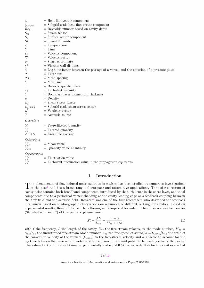
Nowadays a large variety of different hybrid approaches exist differing from each otherin the way the source region is modeled; in the way the equations are used to computethe propagation of acoustic waves in a non-quiescent medium; and in the way the couplingbetween source and acoustic propagation regions is made. This paper intends to makea comparison between some commonly used methods for aero-acoustic applications. Asapplication, the aerodynamically generated noise by a flow over a rectangular cavity isinvestigated. Two different cavities are studied. In the first cavity (L/D = 4, M = 0.5),the sound field is dominated by the wake mode of the cavity, originating from the period-ical vortex shedding at the cavity leading edge, and its higher harmonics. In the secondcavity (L/D = 2, M = 0.6), shear-layer modes, due to flow-acoustic interaction phenom-ena, generate the major components in the noise spectrum. Source domain modeling iscarried out using a second-order finite-volume Large-Eddy simulation (LES), where theeffect of subgrid scale modeling on the accuracy of the final acoustic results is investigated.Propagation equations, taking into account convection and refraction effects, based on ahigh-order finite-difference formulation of the linearized Euler equations (LEE) and acous-tic perturbation equations (APE) are compared with each other using different couplingmethods between source region and acoustic region. Conventional acoustic analogies andKirchhoffs method are rewritten for the different propagation equations and used to ob-tain near-field acoustic results. The accuracy of the different coupling methods and theirsensitivity to the size of the source region is investigated. In this way, this paper aims atgiving more insight in the accuracy and practical use of different hybrid CAA techniquesto predict the aerodynamically generated sound field by a flow over rectangular cavities.

Nomenclature

A = Van Driest damping factorCs = Smagorinsky constantc = Speed of soundcp = Specific heat at constant pressureD = Cavity depthe = Total energy per mass unitf = Frequencyfi = Force componentk = Ratio of the convection velocity of the vortices to the free-stream velocityL = Cavity lengthlη = Kolmogorov length scaleM = Mach numberm = Mode numbern = Normal wall coordinatePrt = Turbulent Prandtl numberp = Pressure

∗PhD. Student, K.U.Leuven, Department of Mechanical Engineering, Celestijnenlaan 300B, 3001 Leuven, Belgium. e-mail:wim.deroeck@mech.kuleuven.be, AIAA Member.

Copyright c© 2005 by the American Institute of Aeronautics and Astronautics, Inc. All rights reserved.

1 of 12

American Institute of Aeronautics and Astronautics Paper 2005-2978

11th AIAA/CEAS Aeroacoustics Conference (26th AIAA Aeroacoustics Conference)23 - 25 May 2005, Monterey, California

AIAA 2005-2978

Copyright © 2005 by the American Institute of Aeronautics and Astronautics, Inc. All rights reserved.

qi = Heat flux vector componentqi,SGS = Subgrid scale heat flux vector componentReD = Reynolds number based on cavity depthSij = Strain tensorSi = Surface vector componentSt = Strouhal numberT = Temperaturet = Timeui = Velocity component−→u = Velocity vectorxi = Space coordinatey+ = Viscous wall distanceα = Lag time factor between the passage of a vortex and the emission of a pressure pulse∆ = Filter size∆xi = Mesh spacingδ = Mesh sizeγ = Ratio of specific heatsµt = Turbulent viscosityθ = Boundary layer momentum thicknessρ = Densityτij = Shear stress tensorτij,SGS = Subgrid scale shear stress tensor−→ω = Vorticity vectorΦ = Acoustic source

Operators

(·) = Favre-filtered quantity

(·) = Filtered quantity< (·) > = Ensemble average

Subscripts

(·)o = Mean value(·)∞ = Quantity value at infinity

Superscripts

(·)′ = Fluctuation value(·)t = Turbulent fluctuation value in the propagation equations

I. Introduction

The phenomenon of flow-induced noise radiation in cavities has been studied by numerous investigationsin the past1 and has a broad range of aerospace and automotive applications. The noise spectrum of

cavity noise contains both broadband components, introduced by the turbulence in the shear layer, and tonalcomponents due to a periodical vortex shedding at the cavity leading edge or a feedback coupling betweenthe flow field and the acoustic field. Rossiter2 was one of the first researchers who described the feedbackmechanism based on shadowgraphic observations on a number of different rectangular cavities. Based onexperimental results, Rossiter derived the following semi-empirical formula for the dimensionless frequencies(Strouhal number, St) of this periodic phenomenon:

St =fL

U∞

=m− α

M∞ + 1/k(1)

with f the frequency, L the length of the cavity, U∞ the free-stream velocity, m the mode number, M∞ =U∞/c∞ the undisturbed free-stream Mach number, c∞ the free-speed of sound, k = Uconv/U∞ the ratio ofthe convection velocity of the vortices (Uconv) to the free-stream velocity and α a factor to account for thelag time between the passage of a vortex and the emission of a sound pulse at the trailing edge of the cavity.The values for k and α are obtained experimentally and equal 0.57 respectively 0.25 for the cavities studied

2 of 12

American Institute of Aeronautics and Astronautics Paper 2005-2978

in the present paper.The different cavities considered in this paper were previously computed using direct numerical simulation

of the Navier–Stokes equations (DNS) by Rowley.3 In the first cavity (4M5) (L/D = 4, with D the depth ofthe cavity and M = 0.5) the sound field is dominated by the wake mode of the cavity, originating from theperiodical vortex shedding at the cavity leading edge, and its higher harmonics. In the second cavity (2M6)(L/D = 2 and M = 0.6) shear-layer modes, due to flow-acoustic interaction phenomena, generate the majorcomponents in the noise spectrum. The Reynolds number of both computations based on the depth of thecavity is 1500 and the ratio L/θo, where θo is the boundary layer momentum thickness at the leading edgeof the cavity due to the initial conditions, is equal to 102 in the case 4M5 and to 52.8 for 2M6.

Although the sound field for this type of applications might be considered as 2D under certain circum-stances,4 the source region should be calculated with a 3D simulation in order not to neglect the inherent3D nature of turbulence. Nevertheless the source calculations in this paper are 2D Large-Eddy Simulations(LES). In this way the largest 2D eddies, which are responsible for the low frequency tonal components, canbe accurately modeled. Broadband components, on the other hand, are generated by the 3D turbulence andwill not be predicted in a precise way. Since the goal of the present paper is to study the accuracy of CAAcomputations with respect to the tonal prediction, a 2D approach is motivated. For the sake of conveniencethe terms LES and unresolved DNS, used in the following parts of the paper refer to the 2D unsteady flowcalculation respectively with and without subgrid scale model.

II. Source region modeling

A. Filtered compressible Navier-Stokes equations

The compressible LES equations for a viscous flow are obtained from a decomposition of the variables ofthe Navier-Stokes equations (ρ, ui) into a Favre-filtered part (ρ, ui) and an unresolved part (ρ′, u′

i) that hasto be modeled with a subgrid scale model (the detailed expressions for the filters and for the subgrid scaleterms can be found for example in Vreman5):

∂ρ

∂t+

∂ρui∂xi

= 0 (2)

∂ρui∂t

+∂ρuiuj∂xj

= − ∂p

∂xi+

∂(τij + τij,SGS)

∂xj(3)

∂ρe

∂t+

∂ρeui∂xi

= −∂uip

∂xi+

∂ui(τij + τij,SGS)

∂xj− ∂(qi + qi,SGS)

∂xi(4)

where ρ, ui and p are the resolved density, velocity components and pressure. For a perfect gas, the totalenergy per mass unit e is defined as p/(γ − 1)ρ+ (u2

1 + u22)/2 with γ the ratio of specific heats. The viscous

stress tensor τij is modeled as a Newtonian fluid, and the heat flux qi is modeled with Fourier’s law. Dynamicmolecular viscosity and molecular conductivity are kept constant.

The subgrid scale tensor τij,SGS , and the subgrid scale heat flux qi,SGS , reproduce the dissipative effectsof the unresolved scales by using a turbulent viscosity µt, and a turbulent Prandtl number Prt, the lastone taken equal to 0.5 for all calculations. The subgrid scale tensor and the heat flux are then modeled asτij,SGS = 2µtSij and qi,SGS = −(µtcp/Prt)∂T /∂xi, with T the temperature and Sij = (1/2)(∂ui/∂xj+∂uj/∂xi)

To determine the turbulent viscosity, a Smagorinsky model is used, where µt = ρ(Cs∆)2√

2Sij Sij . The

Smagorinsky constant Cs is set to 0.1 as suggested in,6 and the filter size ∆ is locally set to the cube root ofthe cell volume. To take into account the scale reduction that occurs near walls, the filter size ∆ is weightedwith the normal wall coordinate y+ in the way proposed by Van Driest: ∆′ = ∆(1 − exp(−y+/A)), withA = 25.

B. Numerical implementation

The filtered compressible Navier–Stokes equations are implemented in a finite-volume code. They are in-tegrated in time using a fourth-order explicit Runge–Kutta scheme. Convective and viscous terms arediscretized using central second-order schemes. On all solid walls, no-slip and no-penetration conditions are

3 of 12

American Institute of Aeronautics and Astronautics Paper 2005-2978

imposed, with ∂p/∂n = 0, n being the direction normal to the wall. At the upstream boundary, characteristicsoft inflow conditions, proposed by Kim and Lee,7 are applied. At the outlet, the subsonic non-reflectingoutflow condition of Poinsot and Lele,8 together with a sponge zone to dissipate vortical structures9 is im-plemented. The top boundary of the domain is located far enough from the cavity to assume that the meanflow values of the primitive variables do not change in the direction normal to this boundary. However, fromthe acoustic point of view, this boundary is too close to the cavity to suppose that the acoustic waves leavethe domain perpendicular to it, as is assumed by Poinsot and Lele,8 for their non-reflecting formulation ofthe boundaries to work properly. The non-perpendicularity of acoustic waves through the top boundary isspecially critical near the top corners of the computational domain. For this reasons, the derivatives of theprimitive variables are set to zero in the top boundary of the domain, and no non-reflecting treatment isapplied there.

C. Discussion of the results

Figure 1 shows the computational domain and indicates several system parameters.

Figure 1. Cavity configuration and computational domain.

A structured multi-block mesh is used for the LES computations. The dimensions of the mesh are700× 130 cells on top of the cavity and 200× 50 inside the cavity for the case 4M5, and 600× 130 cells ontop of the cavity and 100× 50 inside the cavity for the case 2M6 . The mesh is stretched towards the wallsand in the region of the mixing layer. The mesh is also progressively stretched before the outlet region tohelp dissipating vortical structures before they reach the outlet. The mesh size has to be taken sufficientlysmall due to the fact that second-order schemes are used to capture acoustic phenomena. Taking the cavitydepth, D, as the characteristic length of the bigger scales, the Kolmogorov length scale can be estimatedas10 :

D

lη∼ Re

3/4D

The mesh that is used in the present study is approximately of size δ ∼ 8lη. For DNS, the mesh size has tobe δ ≤ 2lη in the free-shear region and y+ ≤ 1 near the walls. The mesh used for the present calculationsis close to that limit, but still belongs to the LES range (LES computations start to be challenging whenδ ∼ 20lη or bigger), hence the subgrid scale model is used. The computations are started from a laminarflat-plate Blasius boundary layer spanning the cavity, and are run until a statistically steady-state is reached.

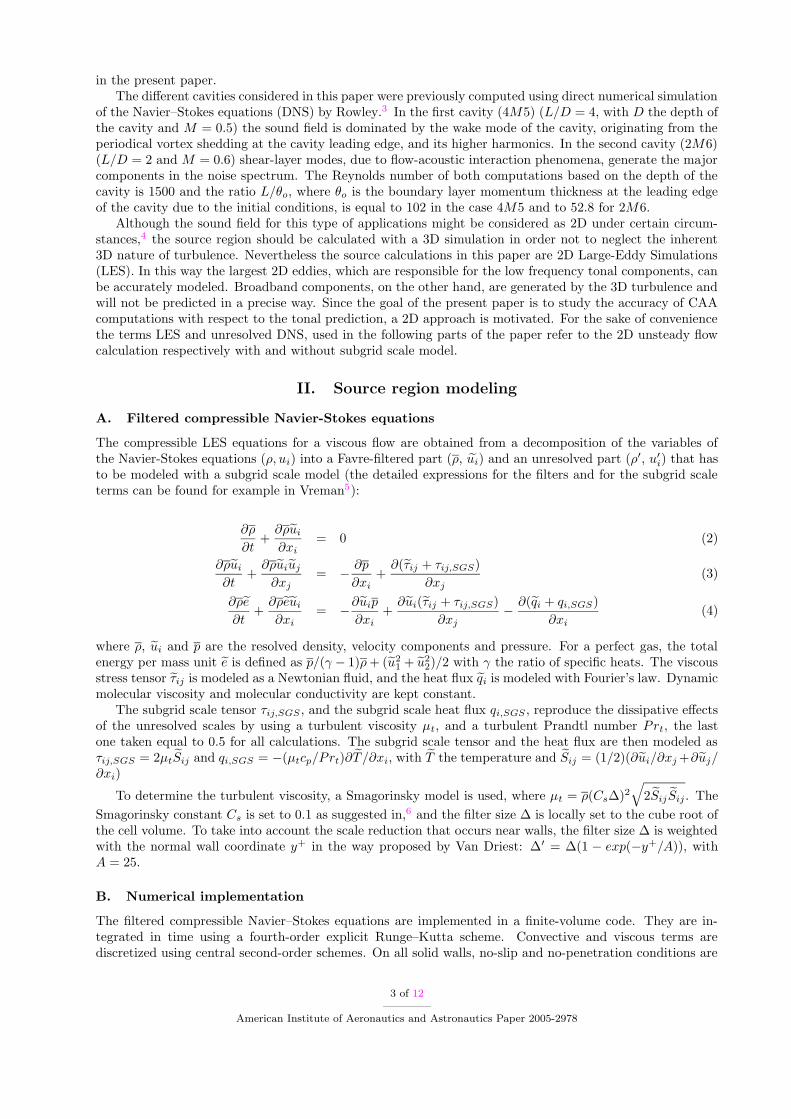
For the cavity oscillating in wake mode (4M5), two different computations have been performed. Oneusing the 2D LES compressible Navier–Stokes equations (2-4), and another one without any subgrid scalemodel (unresolved DNS). For the cavity oscillating in shear mode (2M6), one single computation using theLES equations has been done. Figure 2 shows time-averaged flows for both cavities using the subgrid scalemodel. The streamlines above the cavity are clearly deflected in the wake mode, whereas the shear-layermode shows mean flow streamlines nearly horizontal across the mouth of the cavity. The oscillations in wakemode have a significant impact on the mean flow outside the cavity. It is important to remark that theyaffect the pattern of this mean flow even in the upstream direction. Due to this, the momentum thickness at

4 of 12

American Institute of Aeronautics and Astronautics Paper 2005-2978

the leading edge that is imposed as initial condition is different from the one that is found in the statisticallyconverged flow.

x/D

y/D

-1 0 1 2 3-1

-0.5

0

0.5

1

(a) x/D

y/D

0 2 4-1

-0.5

0

0.5

1

1.5

(b)

Figure 2. Time averaged flow for (a) 2M6 (shear-layer mode) and (b) 4M5 (wake mode).

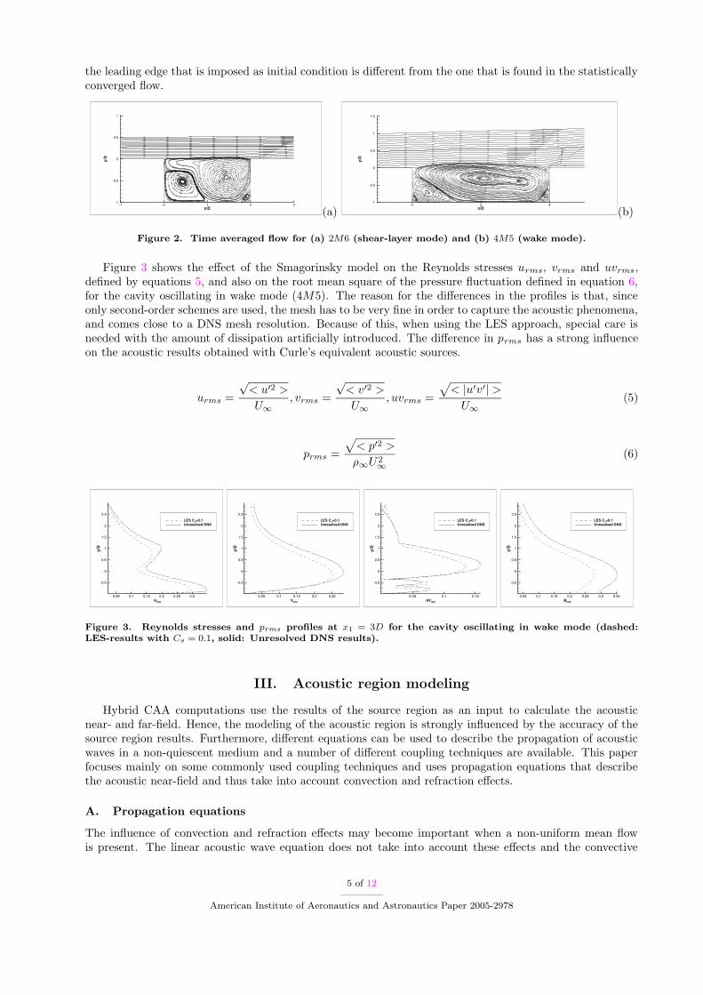
Figure 3 shows the effect of the Smagorinsky model on the Reynolds stresses urms, vrms and uvrms,defined by equations 5, and also on the root mean square of the pressure fluctuation defined in equation 6,for the cavity oscillating in wake mode (4M5). The reason for the differences in the profiles is that, sinceonly second-order schemes are used, the mesh has to be very fine in order to capture the acoustic phenomena,and comes close to a DNS mesh resolution. Because of this, when using the LES approach, special care isneeded with the amount of dissipation artificially introduced. The difference in prms has a strong influenceon the acoustic results obtained with Curle’s equivalent acoustic sources.

urms =

√< u′2 >

U∞

, vrms =

√< v′2 >

U∞

, uvrms =

√< |u′v′| >

U∞

(5)

prms =

√< p′2 >

ρ∞U2∞

(6)

urms

y/D

0.05 0.1 0.15 0.2 0.25 0.3

-0.5

0

0.5

1

1.5

2

2.5

LES Cs=0.1Unresolved DNS

vrms

y/D

0.05 0.1 0.15 0.2 0.25

-0.5

0

0.5

1

1.5

2

2.5

LES Cs=0.1Unresolved DNS

uvrms

y/D

0.05 0.1 0.15

-0.5

0

0.5

1

1.5

2

2.5

LES Cs=0.1Unresolved DNS

prms

y/D

0.05 0.1 0.15 0.2 0.25 0.3 0.35

-0.5

0

0.5

1

1.5

2

2.5

LES Cs=0.1Unresolved DNS

Figure 3. Reynolds stresses and prms profiles at x1 = 3D for the cavity oscillating in wake mode (dashed:LES-results with Cs = 0.1, solid: Unresolved DNS results).

III. Acoustic region modeling

Hybrid CAA computations use the results of the source region as an input to calculate the acousticnear- and far-field. Hence, the modeling of the acoustic region is strongly influenced by the accuracy of thesource region results. Furthermore, different equations can be used to describe the propagation of acousticwaves in a non-quiescent medium and a number of different coupling techniques are available. This paperfocuses mainly on some commonly used coupling techniques and uses propagation equations that describethe acoustic near-field and thus take into account convection and refraction effects.

A. Propagation equations

The influence of convection and refraction effects may become important when a non-uniform mean flowis present. The linear acoustic wave equation does not take into account these effects and the convective

5 of 12

American Institute of Aeronautics and Astronautics Paper 2005-2978

wave equation can only be used when a uniform or irrotational mean flow is present. For this reason, otherequations, based on a decomposition and simplification of the Navier–Stokes equations, are used to calculatethe acoustic near-field propagation. The most commonly used methods to compute the acoustic near-fieldin the presence of a non-uniform mean flow, are the linearized Euler equations (LEE)11 and the acousticperturbation equations (APE).12

The LEE are obtained by decomposing the flow variables (ρ, ui, p) of the Navier-Stokes equations intotheir mean values (ρ0, ui0, p0) and their fluctuating (acoustic) parts (ρ′, u′

i, p′) and by neglecting viscosity

and higher-order terms,

∂ρ′

∂t+

∂

∂xi(ρ′ui0 + ρ0u

′

i) = Φcont (7)

∂ρ0u′

i

∂t+

∂

∂xj(ρ0uj0u

′

i + p′δij) + (ρ′uj0 + ρ0u′

j)∂ui0∂xj

= Φmom,i (8)

∂p′

∂t+

∂

∂xi(ui0p

′ + γp0u′

i) + (γ − 1)(p′∂ui0∂xi

− u′

i

∂p0

∂xi) = Φener (9)

where Φcont,Φmom,i and Φener are the source terms for respectively the continuity, momentum and energyequation, which can contain non-linear, viscosity and temperature effects and can be calculated based ontime-dependent source domain results. The mean flow variables can be easily obtained by calculating theReynolds-Averaged Navies–Stokes equations (RANS).

A major disadvantage of the LEE is the fact that they describe the propagation of acoustic as well asvorticity and entropy waves. If these vorticity and entropy modes are excited by the source terms Φ, this maylead to unphysical or even unstable acoustic solutions for the LEE. For this reason, Ewert and Schroder12

proposed to filter the LEE in Fourier/Laplace space in such a way that the equations only describe thepropagation of acoustic waves. In this way, the APE are obtained, with c0 =

√γp0/ρ0 the mean speed of

sound:

∂p′

∂t+ c20

∂

∂xi[(p′ui0/c

20) + ρ0u

′

i] = Φcont (10)

∂u′

i

∂t+

∂

∂xj[uj0u

′

i + (p′/ρ0)δij ] = Φmom,i (11)

If the source vector Φ only excites only acoustic modes, LEE and APE give a similar solution. Next to thefact that APE only describes the propagation of acoustic waves, another advantage of APE over LEE is thefact that there is no explicit constitutive law equation. So in 2D, only 3 equations have to be solved for eachpoint in the computational domain instead of the 4 equations needed for the LEE

B. Coupling methods

There are two major techniques to couple the source region with the acoustical domain: the techniques usingequivalent aeroacoustic sources and those using acoustic boundary conditions.

1. Acoustic Analogies

There exists a variety of equivalent aeroacoustic source terms which can be calculated from a time-dependantsource region calculation. The different source term formulations are derived by rewriting the Navier–Stokesequations in such a way that the left-hand side contains the propagation equations, used to describe the acous-tic field. The remaining terms in the right-hand side of the equations are treated as equivalent aeroacousticsources Φ. This approach is appealing due to its simplicity and can be used to identify possible aeroa-coustic source phenomena. Furthermore, these methods require less accurate source calculations, since theyare based on aerodynamic fluctuations, and results obtained by incompressible computations or Reynolds-Averaged Navier–Stokes (RANS) calculations (when the turbulent field is stochastically reconstructed11) canbe used.

For low-Mach-number applications with negligible viscosity and temperature effects, the source terms forthe LEE are similar to those proposed by Lighthill,13where the index t refers to the turbulent fluctuating

6 of 12

American Institute of Aeronautics and Astronautics Paper 2005-2978

variables, which are obtained from a time-dependent source calculation:

Φcont = 0

Φmom,i = − ∂∂xj

(ρ0utiu

tj)

Φener = 0

(12)

When the APE are used for this kind of low-Mach-number applications the source terms based on the theoryof vortex sound of Mohring14 can be used as equivalent source:12

{Φcont = 0

Φmom,i = −(−→ω ×−→u )t(13)

The last type of acoustic analogy, used in this paper, is the one proposed by Curle15 to take into account theeffect of solid walls. These source terms are derived by supposing that the forces acting on the walls (whichappear in the right-hand side of the momentum equations) are the dominant sources of sound:

Φcont = 0

Φmom,i = f ti δ(g)

Φener = 0

(14)

with fi = pSi the force acting at the walls, g = 0 defines the solid walls and δ the one-dimensional deltafunction.

2. Acoustic Boundary Conditions

Another way of coupling the results, obtained inside the source region, with the propagation equations,is through the use of acoustic boundary conditions and setting all source terms Φ equal to zero. Thisimposes strong restrictions to the calculation of the source region. Commercial CFD-codes, which solveLES, calculate the flow field with lower-order fairly dissipative numerical schemes without avoiding spuriousreflections at the boundaries. If not taken care of properly, these numerical schemes and boundary conditionscan introduce numerical noise inside the computational domain. These errors can become of the same orderof magnitude as the acoustic variables necessary for this type of coupling.16 All these elements make themethod of acoustic boundary conditions more sensitive to the accuracy of the source region modeling thanthe equivalent sources method.

The acoustic variables that can be used as boundary conditions involve the acoustic pressure and theacoustic velocity. The problem that arises when using this type of acoustic boundary conditions is that thesurface on which the variables are calculated (the Kirchhoff surface), should be located far enough fromthe acoustic sources and no turbulent flow should pass the boundary, such that only acoustic variables canbe taken into account. If outflow occurs at the boundary, the velocity fluctuations may contain vorticitycomponents, and pressure fluctuations may contain hydrodynamic pressure fluctuations, which may excitethe vorticity and entropy modes of the propagation equations and can render unstable solutions. A way ofavoiding these problems is to carry out a filtering of the variables at the Kirchhoff surface in such a waythat only purely acoustic fluctuations are used as boundary conditions. Ovenden and Rienstra17 recentlydeveloped a method to match the flow variables with the acoustic modes of a slowly varying duct. Inthis way, only acoustic variables are taken into account in the propagation equations. Future research willinvestigate the possibility to obtain a more general formulation for this mode matching strategy withoutmaking assumptions on the acoustical duct modes.

The major advantage of the use of acoustic boundary conditions is that, when the boundary variablesonly contain acoustic fluctuations, this method can be seen as an acoustic continuation of the LES in theregions where no further noise sources are present. In this way, it can be assumed that this way of couplingrenders the most accurate results. For this reason, the results obtained with acoustic B.C. are used asreference values in the further part of this paper. Comparison with the DNS-results obtained by Rowley3

confirms these findings. Another advantage of using acoustic B.C. is the fact that the propagation regiondoes not contain the source region and thus a smaller propagation region is needed in which the propagationequations are solved.

7 of 12

American Institute of Aeronautics and Astronautics Paper 2005-2978

In this paper, acoustic pressure boundary conditions are used on a surface surrounding the source region.This may cause vorticity and entropy waves to be present behind the outflow B.C. of the source domain whichmay render in spurious acoustic results in this region. Due to the use of a 7-point stencil finite-differenceimplementation of the acoustic propagation equations, the acoustic pressure surface has a thickness of threepoints. In this way, some additional information about the directivity of the acoustic waves, propagatingthrough the acoustic boundaries, is taken into account.18

C. Numerical implementation

The propagation equations are discretized with a finite-difference method. The space derivatives are calcu-lated with the 4th-order (7-point stencil) dispersion-relation-preserving scheme (DRP).19 In order to filterout spurious high-frequency grid-to-grid oscillations, artificial selective damping20 is added to the equations.Time advancing is carried out with the 5-stage low dispersion-dissipation Runge–Kutta (LDDRK) schemeof Hu et al.21 It was shown in previous research22 that a combination of these numerical schemes gives (forCAA applications) an optimal combination between high accuracy, low dispersion and dissipation errors aswell as reasonable computational efforts.

Three different kinds of boundary conditions (B.C.) must be specified: wall B.C. at the cavity walls,radiation B.C. at the inflow and top boundaries and outflow B.C. at the outflow regions, where vorticity wavesleave the computational domain. The radiation (for acoustic waves that leave the computational domain) andthe outflow B.C. (for acoustic, vorticity and entropy waves that leave the computational domain), derivedby Tam and Dong23 as an asymptotic solution of the LEE, are used. At outflow boundaries a sponge zone9

is added to enhance the non-reflecting performance of this type of B.C.

D. Discussion of the results

The acoustic calculations are carried out on an equidistant Cartesian mesh, containing 321 × 241 nodesoutside the cavity. Inside the cavity respectively 41× 11 and 21× 11 nodes are used for the cavity 4M5 andthe cavity 2M6. The grid size ∆xi is taken equal to 0.1D in both directions. The calculations are carriedout over 11.000 time steps with a CFL-number equal to 1. The results of the last 10.000 time steps are usedto obtain results in the frequency domain. The source region, used for the propagation equation has a heightof 3D and a length of 10D, going from −2.3D to 7.7D with (0, 0) the coordinates at the leading edge of thecavity. In following discussion the Strouhal numbers are all based on the cavity depth.

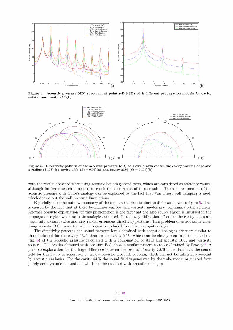
In figure 4 the acoustic pressure spectra are shown for both cavities in a point with coordinates (−D, 8.8D),which corresponds with the point at the angle of 120o shown in the different directivity patterns. The pres-sure spectrum of the cavity 4M5 shows the first resonance frequency due to the the cavity wake mode(St = 0.06) and its higher harmonics. The noise generated by cavity 2M6 is dominated by the shear layermode and results in a dominant first Rossiter mode at Strouhal-number 0.196 and its higher harmonics. TheRossiter frequency is slightly overestimated comparing to the experimental formula (eq.1) which results in aStrouhal number of 0.166 for the first modes. This patterns with similar resonance frequencies (St = 0.063for 4M5 and St = 0.205 for 2M6) are also observed by Rowley.3

1. Propagation Equations

Both LEE and APE give the same results when acoustic boundary conditions are used, due to the fact thatonly acoustic modes are excited. This is especially the case at the inflow and top boundaries since onlyacoustic waves travel through these boundaries, while also vorticity waves and entropy waves may be presentat the outflow boundaries. This explains the small difference observed at the lower angles (< 60o) in thedirectivity patterns of fig.5. The results (both in amplitude and directivity) differ much more when usingacoustic analogies. The main reason for this phenomenon is caused by the different source terms. Whenusing LEE with Lighthill source terms, vorticity and entropy modes may be excited, which are absent in thecase when vorticity based source terms are used in combination with APE.

2. Coupling Methods

Figure 4 compares the sound pressure spectra of the different coupling methods used in this paper for thetwo cavities. Equivalent aeroacoustic sources tend to overestimate the sound pressure levels, as was alreadyobserved in previous research.24 Only Curle’s analogy shows a fairly good agreement in front of the cavity

8 of 12

American Institute of Aeronautics and Astronautics Paper 2005-2978

0 0.05 0.1 0.15 0.2 0.25 0.3 0.35 0.4 0.45 0.50

20

40

60

80

100

120

140

Strouhal Number

Aco

ustic

Pre

ssur

e (d

B)

APE + Acoustic B.C.LEE + Acoustic B.C.APE + Mohring SourcesLEE + Lighthill SourcesAPE + Curle SourcesLEE + Curle Sources

(a)0 0.1 0.2 0.3 0.4 0.5 0.6 0.7

−60

−40

−20

0

20

40

60

80

100

120

Strouhal Number

Aco

ustic

Pre

ssur

e (d

B)

APE + Acoustic B.C.APE + Mohring SourcesAPE + Curle Sources

(b)

Figure 4. Acoustic pressure (dB) spectrum at point (-D,8.8D) with different propagation models for cavity4M5(a) and cavity 2M6(b)

50

100

150

30

60

90

120

150

180 0

APE + Acoustic B.CLEE + Acoustic B.C.APE + Mohring SourcesLEE + Lighthill SourcesAPE + Curle SourcesLEE + Curle Sources

(a)

50

100

150

30

60

90

120

150

180 0

APE + Acoustic B.C.APE + Mohring SourcesAPE + Curle Sources

(b)

Figure 5. Directivity pattern of the acoustic pressure (dB) at a circle with center the cavity trailing edge anda radius of 10D for cavity 4M5 (St = 0.06)(a) and cavity 2M6 (St = 0.196)(b)

with the results obtained when using acoustic boundary conditions, which are considered as reference values,although further research is needed to check the correctness of these results. The underestimation of theacoustic pressure with Curle’s analogy can be explained by the fact that Van Driest wall damping is used,which damps out the wall pressure fluctuations.

Especially near the outflow boundary of the domain the results start to differ as shown in figure 5. Thisis caused by the fact that at these boundaries entropy and vorticity modes may contaminate the solution.Another possible explanation for this phenomenon is the fact that the LES source region is included in thepropagation region when acoustic analogies are used. In this way diffraction effects at the cavity edges aretaken into account twice and may render erroneous directivity patterns. This problem does not occur whenusing acoustic B.C., since the source region is excluded from the propagation region.

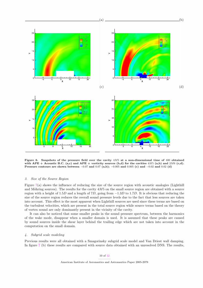
The directivity patterns and sound pressure levels obtained with acoustic analogies are more similar tothose obtained for the cavity 4M5 than for the cavity 2M6 which can be clearly seen from the snapshots(fig. 6) of the acoustic pressure calculated with a combination of APE and acoustic B.C. and vorticitysources. The results obtained with pressure B.C. show a similar pattern to those obtained by Rowley.3 Apossible explanation for the large difference between the results of cavity 2M6 is the fact that the soundfield for this cavity is generated by a flow-acoustic feedback coupling which can not be taken into accountby acoustic analogies. For the cavity 4M5 the sound field is generated by the wake mode, originated frompurely aerodynamic fluctuations which can be modeled with acoustic analogies.

9 of 12

American Institute of Aeronautics and Astronautics Paper 2005-2978

(a) (b)

(c) (d)

Figure 6. Snapshots of the pressure field over the cavity 4M5 at a non-dimensional time of 400 obtainedwith APE + Acoustic B.C. (a,c) and APE + vorticity sources (b,d) for the cavities 4M5 (a,b) and 2M6 (c,d).Pressure contours are shown between −0.07 and 0.07 (a,b); −0.005 and 0.005 (c) and −0.02 and 0.02 (d)

3. Size of the Source Region

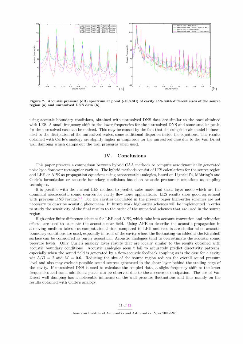
Figure 7(a) shows the influence of reducing the size of the source region with acoustic analogies (Lighthilland Mohring sources). The results for the cavity 4M5 on the small source region are obtained with a sourceregion with a height of 1.5D and a length of 7D, going from −1.3D to 1.7D. It is obvious that reducing thesize of the source region reduces the overall sound pressure levels due to the fact that less sources are takeninto account. This effect is the most apparent when Lighthill sources are used since these terms are based onthe turbulent velocities, which are present in the total source region while source terms based on the theoryof vortex sound are only dominantly present in the vicinity of the cavity.

It can also be noticed that some smaller peaks in the sound pressure spectrum, between the harmonicsof the wake mode, disappear when a smaller domain is used. It is assumed that these peaks are causedby sound sources inside the shear layer behind the trailing edge which are not taken into account in thecomputation on the small domain.

4. Subgrid scale modeling

Previous results were all obtained with a Smagorinsky subgrid scale model and Van Driest wall damping.In figure 7 (b) these results are compared with source data obtained with an unresolved DNS. The results,

10 of 12

American Institute of Aeronautics and Astronautics Paper 2005-2978

0 0.05 0.1 0.15 0.2 0.25 0.3 0.35 0.4 0.45 0.50

20

40

60

80

100

120

140

Strouhal Number

Aco

ustic

Pre

ssur

e (d

B)

Large Source Region: APE + Mohring SourcesSmall Source Region: APE + Mohring SourcesLarge Source Region: LEE + Lighthill SourcesSmall Source Region: LEE + Lighthill Sources

(a)0 0.1 0.2 0.3 0.4 0.5 0.6 0.7 0.8 0.9 1

−20

0

20

40

60

80

100

120

Strouhal Number

Aco

ustic

Pre

ssur

e (d

B)

LES + APE + Acoustic B.C.Unresolved DNS + APE + Acoustic B.C.LES + APE +Curle SourcesUnresolved DNS + APE + Curle Sources

(b)

Figure 7. Acoustic pressure (dB) spectrum at point (-D,8.8D) of cavity 4M5 with different sizes of the sourceregion (a) and unresolved DNS data (b)

using acoustic boundary conditions, obtained with unresolved DNS data are similar to the ones obtainedwith LES. A small frequency shift to the lower frequencies for the unresolved DNS and some smaller peaksfor the unresolved case can be noticed. This may be caused by the fact that the subgrid scale model induces,next to the dissipation of the unresolved scales, some additional disperion inside the equations. The resultsobtained with Curle’s analogy are slightly higher in amplitude for the unresolved case due to the Van Driestwall damping which damps out the wall pressures when used.

IV. Conclusions

This paper presents a comparison between hybrid CAA methods to compute aerodynamically generatednoise by a flow over rectangular cavities. The hybrid methods consist of LES calculations for the source regionand LEE or APE as propagation equations using aeroacoustic analogies, based on Lighthill’s, Mohring’s andCurle’s formulation or acoustic boundary conditions based on acoustic pressure fluctuations as couplingtechniques.

It is possible with the current LES method to predict wake mode and shear layer mode which are thedominant aeroacoustic sound sources for cavity flow noise applications. LES results show good agreementwith previous DNS results.3,6 For the cavities calculated in the present paper high-order schemes are notnecessary to describe acoustic phenomena. In future work high-order schemes will be implemented in orderto study the sensitivity of the final results to the order of the numerical schemes that are used in the sourceregion.

High-order finite difference schemes for LEE and APE, which take into account convection and refractioneffects, are used to calculate the acoustic near field. Using APE to describe the acoustic propagation ina moving medium takes less computational time compared to LEE and results are similar when acousticboundary conditions are used, especially in front of the cavity where the fluctuating variables at the Kirchhoffsurface can be considered as purely acoustical. Acoustic analogies tend to overestimate the acoustic soundpressure levels. Only Curle’s analogy gives results that are locally similar to the results obtained withacoustic boundary conditions. Acoustic analogies seem t fail to accurately predict directivity patterns,especially when the sound field is generated by a flow-acoustic feedback coupling as is the case for a cavitywit L/D = 2 and M = 0.6. Reducing the size of the source region reduces the overall sound pressurelevel and also may exclude possible sound sources generated in the shear layer behind the trailing edge ofthe cavity. If unresolved DNS is used to calculate the coupled data, a slight frequency shift to the lowerfrequencies and some additional peaks can be observed due to the absence of dissipation. The use of VanDriest wall damping has a noticeable influence on the wall pressure fluctuations and thus mainly on theresults obtained with Curle’s analogy.

11 of 12

American Institute of Aeronautics and Astronautics Paper 2005-2978

Acknowledgements

The research work of Wim De Roeck and Yves Reymen is financed by a scholarship of the Institute forthe Promotion of Innovation by Science and Technology in Flanders (IWT).

References

1Komerath, N. M., Ahuja, K. K., and Chambers, F. W., “Prediction and Measurement Flows over Cavities - a survey,”Aiaa-paper 82-022, 1987.

2Rossiter, J. E., “Wind Tunnel Experiments on the Flow over Rectangular Cavities at Subsonic and Transonic Speeds,”Royal aircraft establishment, techical report 64037, 1964.

3Rowley, C. W., Modeling, Simulation, and Control of Cavity Flow Oscillations, Ph.D. thesis, California Institute ofTechnology, Pasadena, California, 2002.

4Ahuja, K. K. and Mendoza, J., “Effects of Cavity Dimensions, Boundary Layer, and Temperature on Cavity Noise withEmphasis on Benchmark Data to Validate Computational Aeroacoustic Codes,” Nasa cr, techical report 4653, 1964.

5Vreman, B., Direct and Large-Eddy Simulation of the Compressible Turbulent Mixing Layer , Ph.D. thesis, Departmentof Applied Mathematics, University of Twente, Enschede, The Netherlands, 1995.

6Gloerfelt, X., Bogey, C., and Bailly, C., “Numerical Evidence of Mode Switching in the Flow-induced Oscillations by aCavity,” International Journal of Aeroacoustics, Vol. 2, 2003, pp. 99–124.

7Kim, J. W. and Lee, D. J., “Generalized Characteristic Boundary Conditions for Computational Aeroacoustics,” AIAAJournal , Vol. 38, 2000, pp. 2040–2049.

8Poinsot, T. J. and Lele, S. K., “Boundary Conditions for Direct Simulations of Compressible Viscous Flow,” Journal ofComputational Physics, Vol. 101, 1992, pp. 104–129.

9Colonius, T., Lele, S. K., and Moin, P., “Boundary Conditions for Direct Computation of Aerodynamic Sound,” AIAA-journal , Vol. 31, 1993, pp. 1574–1582.

10Pope, S. B., Turbulent Flows, Cambridge University Press, 2000.11Bailly, C. and Juve, D., “Numerical Solution of Acoustic Propagation Problems Using Linearized Euler Equations,”

AIAA-journal , Vol. 38, 2000, pp. 22–29.12Ewert, R. and Schroder, W., “Acoustic Perturbation Equations Based on Flow Decomposition via Source Filtering,”

Journal of Computational Physics, Vol. 188, 2003, pp. 365–398.13Lighthill, M. J., “On Sound Generated Aerodynamically; I. General Theory,” Proc. Roy. Soc. (London), Vol. 211, 1952,

pp. 564–587.14Mohring, W., “On Vortex Sound at Low Mach Number,” Journal of Fluid Mechanics, Vol. 85, 1978, pp. 685–691.15Curle, N., “The Influence of Solid Boundaries upon Aerodynamic Sound,” Proc. Roy. Soc. (London), Vol. 231, 1955,

pp. 505–514.16Tam, C. K. W., “Computational Aeroacoustics: Issues and Methods,” AIAA-Journal , Vol. 33, 1995, pp. 1788–1796.17Ovenden, N. C. and Rienstra, S., “Mode-Matching Stategies in Slowly Varying Engine Ducts,” AIAA-Journal , Vol. 42,

2004, pp. 1832–1840.18Terracol, M., Manoha, E., Herrero, C., and Sagaut, P., “Airfoil Noise Predictions Using Large Eddy Simulations, Euler

Equations and Kirchhoff,” Proceedings LES for Acoustics Conference, DGLR, Gottingen, Germany, 2002.19Tam, C. K. W. and Webb, J. C., “Dispersion-Relation-Preserving Schemes for Computational Aeroacoustics,” Proceedings

of 14th DGLR/AIAA Aeroacoustics Conference, DGLR/AIAA, Aachen, Germany, 1990.20Tam, C. K. W., Webb, J. C., and Dong, Z., “A Study of the Short Wave Components in Computational Acoustics,”

Journal of Computational Acoustics, Vol. 1, 1993, pp. 1–30.21Hu, F. Q., Hussaine, M. Y., and Manthey, J. L., “Low-Dissipation an Low Dispersion Runge-Kutta Schemes for Compu-

tational Aeroacoustics,” Journal of Computational Physics, Vol. 124, 1996, pp. 177–191.22De Roeck, W., Desmet, W., Baelmans, M., and Sas, P., “An Overview of High-Order Finite Difference Schemes for

Computational Aeroacoustics,” Proceedings of the International Conference on Sound and Vibration, ISMA 2004 , K.U. Leuven,Leuven, Belgium, 2004, pp. 353–368.

23Tam, C. K. W. and Dong, Z., “Radiation and Outflow Boundary Conditions for Direct Computation of Acoustic andFlow Disturbances in a Nonuniform Mean Flow,” Journal of Computational Acoustics, Vol. 4, 1996, pp. 175–201.

24De Roeck, W., Desmet, W., Baelmans, M., and Sas, P., “On the prediction of near-field cavity flow noise using differentCAA techniques,” Proceedings of the International Conference on Sound and Vibration, ISMA 2004 , K.U. Leuven, Leuven,Belgium, 2004, pp. 369–388.

12 of 12

American Institute of Aeronautics and Astronautics Paper 2005-2978