Machine Learning Techniques for Downscaling SMOSSatellite Soil Moisture Using MODIS Land SurfaceTemperature for Hydrological Application

Prashant K. Srivastava & Dawei Han & Miguel Rico Ramirez & Tanvir Islam

Received: 8 January 2013 /Accepted: 21 March 2013 /Published online: 18 April 2013# Springer Science+Business Media Dordrecht 2013

Abstract Many hydrologic phenomena and applications such as drought, flood, irrigationmanagement and scheduling needs high resolution satellite soil moisture data at a local/regionalscale. Downscaling is a very important process to convert a coarse domain satellite data to afiner spatial resolution. Three artificial intelligence techniques along with the generalized linearmodel (GLM) are used to improve the spatial resolution of Soil Moisture and Ocean Salinity(SMOS) derived soil moisture, which is currently available at a very coarse scale of ~40 Km.Artificial neural network (ANN), support vector machine, relevance vector machine andgeneralized linear models are chosen for this study to integrate the Moderate ResolutionImaging Spectroradiometer (MODIS) Land Surface Temperature (LST) with the SMOS de-rived soil moisture. Soil moisture deficit (SMD) derived from a hydrological model called PDM(Probability Distribution Model) is used for the downscaling performance evaluation. Thestatistical evaluation has also been made with the day-time and night-time MODIS LSTdifferences with the mean day and night-time PDM SMD data for the selection of effectiveMODIS products. The accuracy and robustness of all the downscaling algorithms are discussed interms of their assumptions and applicability. The statistical performance indices such as R2,%Biasand RMSE indicates that the ANN (R2=0.751, %Bias=−0.628 and RMSE=0.011), RVM(R2=0.691, %Bias=1.009 and RMSE=0.013), SVM (R2=0.698, %Bias=2.370 andRMSE=0.013) and GLM (R2=0.698, %Bias=1.009 and RMSE=0.013) algorithms on thewhole are relatively more skillful to downscale the variability of the soil moisture in comparisonto the non-downscaled data (R2=0.418 and RMSE=0.017) with the outperformance of ANNalgorithm. The other attempts related to growing and non-growing seasons have been used inthis study to reveal that season based downscaling is even better than continuous time serieswith fairly high performance statistics.

Keywords Soil moisture . SMOS . Soil moisture deficit . Artificial intelligence .

Support vector machine . Relevance vector machine . Artificial neural network .

Generalized linear models

Water Resour Manage (2013) 27:3127–3144DOI 10.1007/s11269-013-0337-9

P. K. Srivastava (*) : D. Han :M. R. Ramirez : T. IslamWater and Environment Management Research Centre, Department of Civil Engineering,University of Bristol, Bristol, BS8 1TR, UKe-mail: cepks@bristol.ac.uk

1 Introduction

Soil moisture in the top Earth’s surface has been widely recognised as a key variable innumerous environmental studies including meteorology, hydrology, agriculture, and climatechange (Mladenova et al. 2011; Jackson 1993). With the latest satellites, the retrieval of soilmoisture is now possible at a coarser spatial resolution. However, its accurate retrieval up toa finer spatial resolution by downscaling is very much important (Piles et al. 2011; Pancieraet al. 2008; Merlin et al. 2008). Soil moisture is very difficult to observe with in situmeasurements at large scales due to its large spatial and temporal variability, and its variationwithin the vertical soil profile (Al-Shrafany et al. 2012a; Al-Shrafany et al. 2012b). Wagneret al. (2007) indicates that remote sensing of surface soil moisture has the potential to helpfill this gap. In addition, Piles et al. (2011) shows that the downscaling of soil moisture isnecessary for finer spatial applications.

The European Space Agency Soil Moisture and Ocean Salinity (SMOS) mission and theforthcoming Soil Moisture Active Passive (SMAP) mission, to be launched in 2014, aredesigned to provide global measurements of the near-surface soil moisture. However, forregional applications, the downscaling of these data with other higher resolution data derivedfrom optical sensors could be used to bring it to a higher resolution for application over acatchment scale. Numerous researchers have used the optical sensors for soil moistureestimation in the past, since optical sensors provide a very high spatial resolution data.Some of the techniques like the Universal triangle method have been used in practicalexamples (Carlson 2007; Mallick et al. 2009; Sandholt et al. 2002). It has been proven thatthe abovementioned methods are based on atmospheric and terrestrial physics and quitesensitive to soil hydro-geo-environment. Previous studies have shown that the variation insoil moisture can be directly linked with land surface temperature and NDVI (Sandholt et al.2002; Goward et al. 2002). Hence, high resolution optical sensors based on MODIS landsurface temperature (LST) could be a suitable choice for downscaling experiments. In thisstudy, several attempts have been made to synergistically combine the SMOS soil moistureestimates and the MODIS LST data to downscale the SMOS soil moisture through theartificial intelligence (AI) techniques because there is a lack of information in the publishedliterature on such a study.

Artificial intelligence (AI) algorithms such as Support Vector Machine (SVM), RelevanceVector machine (RVM) and Artificial Neural Network (ANN) are used here to downscaleSMOS soil moisture. Generalized Linear Models (GLM) is also used, as it is a leastcomputationally demanding technique and provides useful results (Weichert and Bürger1998; Trigo and Palutikof 2001; Schoof and Pryor 2001). ANNs are one of the verypowerful mathematical tools and have been successfully used in hydrology for tacklingmany modelling problems like river level forecasting, rainfall runoff modelling, dailyevaporation, sedimentation yield, rainfall forecasting, ground water modelling, reservoirinflow, water quality prediction and water resources management (Han et al. 2007;Srivastava et al. 2012b; Islam et al. 2012). Conjunction models with ANNs are quite popularin the field of hydrology and earth sciences (Wu and Chau 2011; Ishak et al. 2013). TheANN is a reliable tool to improve the estimation of hydrological and meteorological vari-ables such as wind speed, net radiation, relative humidity, air temperature, precipitation ratesand atmospheric pressure (Wang et al. 2011). Another useful tool in hydrology from theMachine Learning community field is called a Support Vector Machine (SVM) and hasgained considerable attention in hydrology, meteorology and related fields (Han and Yang2001; Han and Cluckie 2004). Apart from SVM, a sparse Bayesian probabilistic learningframework based Relevance Vector machine (RVM) developed by Tipping (2001) is also

3128 P.K. Srivastava et al.

used in this study which is found to have some advantages over SVM (Foody 2008; Bishopand Tipping 2000; Ghosh and Mujumdar 2008; Tipping 2001). These artificial intelligencetechniques have many merits over traditional modelling techniques due to their better abilityto handle enormous amounts of noisy data from dynamic and non-linear systems (Remesanet al. 2009; Sivapragasam and Muttil 2005).

The foremost objective of this research is on the application of GLM, ANN and RVM forevaluating their downscaling capabilities of the SMOS soil moisture through the soilmoisture deficit derived from Probability Distribution Model (PDM) over the Brue catch-ment, Southwest of England measured at the time closest to SMOS overpass. The fourtechniques used will further elaborate the comparable performance GLM, SVM, RVM andANN towards downscaling of SMOS soil moisture. The other attempts have been made inthis study are based on downscaling of growing and non-growing season datasets. Details ofthe SMOS, MODIS, and ground-based data used in this study are presented in Section 2.The downscaling methodologies are also fully described in this section. Results and discus-sion of all the AI techniques used for the SMOS downscaling and season discriminateddatasets are provided in Section 3 along with the statistical performances.

2 Materials and Methodology

2.1 Study Area

The Brue catchment (135.5 Km2) is chosen as the study area which is located in the south-west of England, 51.11 °N and 2.47 °W. The major land use is pasture land on clay soil withsome patches of woodland in the higher eastern catchment. The land use/land cover of Brueis illustrated in Fig. 1 with the topography and ground station locations. It is a predominantlya pasture land with modest relief. The ground observed hourly data for this study areobtained from the NERC (Natural Environment Research Council) for the given period.The meteorological datasets are provided by the British Atmospheric Data Centre (BADC)that includes wind, net radiation, surface temperature and dew point and used for thereference Evapotranspiration estimation used as a input in PDM (Srivastava et al. 2013b).The observed hourly rain gauge and river flow data for this study are obtained from theEnvironment Agency (U.K.). The observations covers a total 12 months period fromFebruary 2011 to January 2012, from which the first 8 months are used for the calibrationand the remaining 4 months, are utilized for the validation purposes.

2.1.1 The MODIS and SMOS Products

The MODIS (Moderate Resolution Imaging Spectroradiometer) is a key instrument aboard theTerra and Aqua satellites. It has a viewing swath width of 2,330 km and views the entire surfaceof the Earth every one to two days. Its detectors measure 36 spectral bands between 0.405 and14.385 μm, and it acquires data at three spatial resolutions 250 m, 500 m, and 1,000 mrespectively while the high level MODIS Land Products distributed from LP DAAC areproduced at four nominal spatial resolutions including 5,600 m (0.05 degrees). MODIS hasbeen selected among other operational optical satellites for its suitable characteristics, mostly,due to its daily temporal resolution and free near real time data availability (Thakur et al. 2012).Both day-time and night-time passes are provided once per day at each grid box for cloud freepixels. TheMODIS Level 3 (~5.6 km) LST data are gridded uniformly across the globe. Hence,for the downscaling the MODIS land surface temperature (LST) level 3 product with a

Machine Learning Techniques for Downscaling SMOS 3129

multitude of SMOS soil moisture are used. In order to use the MODIS Terra level 3 LST day-time product, we averaged the data using the Brue boundary using ENVI ITT version 4.8 andthen determine the mean available MODIS observation over the Brue catchment. Attemptshave also been made to use ΔLST for the downscaling purposes (LSTday-LSTnight) but due to itspoor performance with the soil moisture deficit (SMD) in comparison to LSTday, the datasetshas not been considered for the downscaling (see Fig. 4b).

The SMOS mission is a joint program of the European Space Agency (ESA), the NationalCentre for Space Studies (CNES - Centre National d’Etudes Spatiales), and the IndustrialTechnological Development Centre (CDTI – Centro para el Desarrollo TechnológicoIndustrial). The MIRAS instrument in the SMOS satellite acquires data at the frequency of1.4 GHz (L-band) and is a dual polarized 2-D interferometer and is the first-ever, polar-orbiting,space-borne, 2-D interferometric radiometer designed to provide global information on surfacesoil moisture with an accuracy of 4 % (Kerr et al. 2001). In this study, Level 2 SMOS soilmoisture products are used. This L2 soil moisture product is based on an iterative approachwhich aims at minimizing a cost function. The end user Level 2 SM product contains soilmoisture, vegetation opacity, estimated dielectric constant and brightness temperature comput-ed at 42.5° (Kerr et al. 2012). More details of SMOS L2 products and algorithm are given inSMOS level 2 processor soil moisture algorithm theoretical basis document (ATBD) (Kerr et al.2006). The SMOS soil moisture products are defined on the ISEA 4H9 grid i.e. IcosahedralSnyder Equal Area projection with aperture 4, resolution 9 and its shape of cells as hexagon

Fig. 1 Geographical location of the study area with observation stations and land use/land cover overlaid overdigital elevation model

3130 P.K. Srivastava et al.

(Pinori et al. 2008). The radiometric resolution of the instrument is ~40 km with the soilmoisture retrieval unit in m3 m−3 (i.e. volumetric). The instrument provides records of bright-ness temperatures over incidence angles from 0° up to 55° across a 600 km swath (Pinori et al.2008). Each point (or node) of this grid is known as a DGG (Discrete Global Grid) with fixedcoordinates and is assigned with an identificator the “DGG Id”. For the comparison between thecatchment and SMOS soil moisture, the SMOS pixel with its centroid over the catchment isextracted and considered for the subsequent analysis. The Beam 4.9 package with SMOS 2.1.3plugin is used for the data extraction. The SMOS data is freely available and can be downloadedfrom the SMOS website free of cost with minimal formalities:

http://www.esa.int/Our_Activities/Observing_the_Earth/The_Living_Planet_Programme/Earth_Explorers/SMOS

2.2 Artificial Intelligence Techniques and GLM

The AI techniques and GLM used in this study are briefly explained in the subsections withtheir theoretical backgrounds. All the AI techniques and GLM are employed through Rprogramming language, an open source software developed for statistical computing andgraphics (RDevelopment 2010).

2.2.1 Support Vector Machine (SVM)

The SVMs for regression were first introduced by Vapnik et al. in (1997). SVMs can berepresented as two-layer networks (where the weights are non-linear in the first layer and linearin the second layer). Mathematically, a basic function for the statistical learning process is

y ¼ f ðxÞ ¼XM

i¼1aiϕiðxÞ ¼ wϕðxÞ ð1Þ

where the output is a linearly weighted sum ofM. The nonlinear transformation is carried out by8(x).

The decision function of SVM is represented as

y ¼ f ðxÞ ¼XN

i¼1aiK xi; xð Þ

n o� b ð2Þ

where K is the kernel function, αi and b are parameters, N is the number of training data, xiare vectors used in the training process and x is the independent vector. The parameters αi

and b are derived by maximising their objective function. The least squares approach is usedto choose the parameters (w, b) to minimise the sum of the squared deviations of the data.The approach called as ε -SV regression is used in this study. The role of the kernel functionsimplifies the learning process by changing the representation of the data. In this study, theradial based function has been used. The deviation between the target value and the functiondescribing the hypothesis found by the support vector machine is controlled by the ε parameter.The optimised values of cost function are discussed briefly in Section 3.1. The R “kernlab”package has been used in this study for SVM implementation (Karatzoglou et al. 2005).

2.2.2 Relevance Vector Machine

Tipping (2001) proposed the relevance vector machine (RVM) in a Bayesian context. FromBishop and Tipping (2000) and Tipping (2001), the RVMmodel is based on probabilistic theoryoperated by a set of hyperparameters associated with weights, whose most probable values are

Machine Learning Techniques for Downscaling SMOS 3131

iteratively estimated from the data. The training vectors associated with nonzero weights aretermed as relevance vectors. The most compelling feature of the RVM is that, while itsgeneralisation performance is comparable to an equivalent SVM, it typically utilizes dramaticallyfewer kernel functions. The mathematical background of RVM is presented briefly in (Tipping2001). The RVM model variable can be characterised by the equations depicted below.

y ¼ f ðxÞ þ "n where "n � N 0;σ2"n

� �ð3Þ

p y w;σ2"n

��� �¼ 2pσ2

"n

� ��l 2=exp � 1

2σ2"n

y� 6wk k2( )

ð4Þ

where, w ¼ w0;w1; . . . . . . ;wlð ÞT and 6 xið Þ ¼ 1;K xi; x1ð Þ;K xi; x2ð Þ; . . . :;K xi; xlð Þ½ �T . Max-imum likelihood estimation of w and σ2

"nis often associated with over fitting problem. To

overcome this problem, Tipping (2001) recommended the addition of a complex penalty tothe likelihood or error function.

In comparison to SVM, RVM doesn’t make unnecessarily liberal use of basis functions.The predictions of RVM are probabilistic, while SVM produces point estimates. There is nostraightforward method to estimate C and ε in SVM. Optimization for those variables isinefficient for both data and computation. The kernel function K(x,xi) must satisfy Mercer’scondition. In RVM, a fully probabilistic framework is adopted with a priori over the modelweights governed by a set of hyperparameters, associated with weights, whose most probablevalues are iteratively estimated from the data. Sparsity is achieved because in practice theposterior distributions of many of the weights are sharply (indeed infinitely) peaked aroundzero. In this study the Gaussian radial basis kernel function is adopted. The optimised values ofsigma hyperparameters are discussed briefly in Section 3.1. The R “kernlab” package has beenused in this study for RVM implementation (Karatzoglou et al. 2005).

2.2.3 Artificial Neural Network (ANN)

This study has adopted the artificial neural network with the Levenberg-Marquardt trainingwith the architecture 2-2-1 network. The activation function of the hidden layer is sigmoidand the output layer is purelin. There is an extra input assumed to have a constant value ofone and the weight that modifies this extra input is called the bias. The structure of the ANNemployed is shown in Fig. 2. For the output layer, a linear function is used with the relevantcalculations as follows (Anderson and Davis 1995):

Oa ¼ hhiddenXPp¼1

ia;pwa;p þ ba

!ð5Þ

where

hhiddenðxÞ ¼ 1

1þ e�xð6Þ

In the above equation, Oa is the output of the current hidden layer node a, P is the numberof nodes in the previous hidden layer, ia,p is an input to node a from either the previoushidden layer p or network input p, wa,p is the weight modifying the connection from either’rnode p to node a or from input p to node a, and ba is the bias. In the above equation, hhidden

3132 P.K. Srivastava et al.

(x) is the sigmoid activation function of the node (Ishak et al. 2013). In ANN, an appropriatenormalisation of the training data is essential to avoid saturating the activation function,which is done to restrict their ranges within the interval of −1 to 1. The following normaliseequation is used (Zhang et al. 1998):

znorm ¼ zo � z

zmax � zminð7Þ

where znorm = normalised value; z0 = original value; z = mean; zmax = maximum value; andzmin = minimum value. The best parameter values for decay rate, hidden layers and iterationsare discussed briefly in Section 3.1. The R “nnet” package has been used in this study forANN implementation (Ripley 2009).

2.2.4 Generalized Linear Model (GLM)

Generalized linear models (GLMs) are a large class of statistical models for relating re-sponses to linear combinations of predictor variables, including many commonly encoun-tered types of dependent variables and error structures as special cases (Lindsey 1997). Onevariable is considered to be an explanatory variable (xi), and the other is considered to be adependent variable (yi) (Johnson and Wichern 2002). They are represented as

yi ¼ xibþ ei; ð8Þwhere i=1, . . . , n,; yi is a dependent variable, xi is a vector of k independent predictors, b is avector of unknown parameters and the ei is stochastic disturbances. GLM models arecharacterized by stochastic component, systematic component and link between the random andsystematic components (McCullagh and Nelder 1989). For a normal linear model xib is an identityfunction of the mean parameter, while GLM is governed by some link function. The variance andlink function used in this study are all belongs to Gaussian family with link = “identity”.

2.3 Season Based Downscaling

Remote sensing studies have shown that plant canopy cover has an important impact onsatellite soil moisture remote sensing (Ridler et al. 2012; Legates et al. 2011). In this study, toexplore the influence of canopy cover, further data analysis is divided into growing and non-growing seasons. In the United Kingdom, the growing season starts when the temperature onfive consecutive days exceeds 5°C. Therefore, in this study the whole winter season

Fig. 2 Structure of the ANN used in this study (Input 1 and 2 are the MODIS LST and SMOS soil moisturevariables while Output is PDM SMD)

Machine Learning Techniques for Downscaling SMOS 3133

(December–February) is taken as the non-growing season (average temperature <5°C) andMarch to November is selected as the growing season (average temperature >5°C) (Source:http://www.metoffice.gov.uk/climate/uk/averages/ukmapavge.html). After separating thedatasets, the best model is applied (selected from algorithms performances) to downscalethe SMOS soil moisture using the LST. Later on, the two algorithms are merged together andtested with the final validation datasets.

2.4 Probability Distributed Model (PDM)

The PDM is a fairly general conceptual rainfall-runoff model which transforms rainfall andevaporation data to flow at the catchment outlet (Moore 2007; Liu and Han 2010). The PDMhas been widely applied throughout the United Kingdom and world, both for operational anddesign purposes (Moore 2007). In this study, the PDM is used for SMD estimation throughits moisture deficit routine. The SMD routine is based on (Moore 2007):

E0i

Ei¼ 1� Smax � SðtÞð Þ

Smax

� �be

ð9Þ

where E0i

Eiis the ratio of actual ET to potential ET; be is exponent in actual evaporation

function and Smax � SðtÞð Þ is Soil Moisture Deficit; Smax is the total available storage andS(t) is storage. The calibration and validation of PDM model and SMD are discussed brieflyby (Srivastava et al. 2012a; 2013a).

2.5 Statistical Parameters

In this study we compared the various downscaled values of soil moisture with the PDM soilmoisture deficit. The performances between two patterns are quantified in terms of the Nash-Sutcliffe Efficiency (R2), the Root Mean Square Error (RMSE) and the percentage of bias(%Bias). The percentage of bias measures the average tendency of the simulated values to belarger or smaller than their observed ones. The optimal value of %Bias is 0.0, with low-magnitude values indicating accurate model simulation (Eq. 10). Positive values indicateoverestimation bias, whereas negative values indicate model underestimation bias. The R2 isbased on the sum of the absolute squared differences between the simulated and observedvalues normalised by the variance of the observed values during the investigation period. R2 iscalculated using Eq. 11 while Root Mean Square Error (RMSE) can be calculated using Eq. 12.

%Bias ¼ 100 �X

yiðiÞ � xiðiÞð ÞX

xiðiÞð Þ.h i

ð10Þ

R2 ¼ 1�Pni¼1

yiðiÞ � xiðiÞ½ �2

Pni¼1

xiðiÞ � xi½ �2ð11Þ

RMSE ¼ffiffiffiffiffiffiffiffiffiffiffiffiffiffiffiffiffiffiffiffiffiffiffiffiffiffiffiffiffiffiffiffiffiffiffiffiffiffiffiffiffiffiffiffiffiffiffi1

n

Xni¼1

yiðiÞ � xiðiÞ½ �2 !vuut ð12Þ

where n is the number of observations; x is the Observed variable and y is the Simulated variable.

3134 P.K. Srivastava et al.

3 Results and Discussions

3.1 Optimisation of the AI Techniques

The AI techniques parameters need to be optimised for a stable result and thus requirea preliminary analysis of parameters before using it for computational downscaling. Inthis study, we began with a very small network and varied several parameters includingthe number of hidden layers, number of nodes in the hidden layer, and learningmomentum for obtaining the best parameters for downscaling. We consider modelselection of RVM and SVM, subsuming hyperparameter adaptation and feature selectionwith respect to different model selection criteria. This type of trial-and-error approach iscommonly employed for selection of best parameters for any artificial intelligencetechniques. In this work, automatic hyperparameter estimation has been done whichuses the heuristics in sigest module to calculate a good sigma value for the Gaussianradial based function. The “sigest” estimates the range of values for the sigma param-eter which would return good results (Caputo et al. 2002). The estimation is based uponthe 0.1 and 0.9 quantile of \|x−x′\|^2. Basically any value in between those two boundswill produce good results. More detail about “sigest” is given over RCran web (http://cran.r-project.org/web/packages/kernlab/kernlab.pdf). The hyperparameter sigma valuefor RVM is 0.494 with training error 0.000 are obtained. There are 22 relevance vectorsgenerated during the simulation. In case of SVM at epsilon = 0.1, the optimised costfunction C = 1 and hyperparameter sigma are found to be 1.22 with the training errorof 0.164 and objective function −46.95. The number of support vectors retrieved duringthe model simulation is recorded as 158 (Table 1). Neural network training is oftenperformed by trying to minimize the total error or, equivalently, the average error forthe training set, generally expressed as a function of the weights. Nevertheless, mini-mizing training error can lead to overfitting and thus poor generalization. A commonapproach to improve generalization error is regularization, which can be employed by

Table 1 SVM performance with different cost function (C)

C at epsilon = 0.1 Objective function Training error Sigma value #Support vectors

0.001 −0.17 1.12 1.89 218

0.01 −1.58 0.80 1.91 213

0.1 −8.64 0.25 1.26 167

1 −46.95 0.16 1.22 156

10 −371.84 0.16 1.02 155

Table 2 ANN performance withdifferent weight decay ratefunction

Decay rate RMSE (m)

5×10−5 0.011

5×10−4 0.011

5×10−3 0.012

0.05 0.019

0.5 0.046

5.0 0.112

Machine Learning Techniques for Downscaling SMOS 3135

using a weight decay function (Moody et al. 1995). For this reason to estimate thepromising value of decay function, its optimization is taken into consideration. InTables 2 and 3 the parameterisation of ANN with respect to weight decay rate showsthat 5×10−4 is sufficient for the architecture used in this study while the number ofiterations during the neural network simulations indicates that the performance of ANNgets saturated after 1,000 iterations, hence this can be used as an optimal value forANN simulations (Fig. 3). Previous research shows that increase in the number ofhidden layers has effect on the performance of ANN, however after 2 hidden layersperformance gets saturated (Zhang et al. 1996). Therefore 2 hidden layers are used inthis study. However, in case of computational speed problems one hidden layer is alsosufficient for the optimal performance of ANN (Gao 2008).

Table 3 ANN performancewith different iterations (hiddenlayers = 2)

Iterations RMSE (m)

10 0.065

100 0.012

1000 0.010

10000 0.010

100000 0.010

Fig. 3 Performance of ANN with different decay rate and iterations

3136 P.K. Srivastava et al.

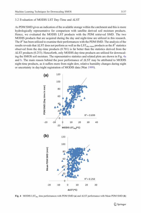
3.2 Evaluation of MODIS LST Day-Time and ΔLST

As PDMSMDgives an indication of the available storage within the catchment and this is morehydrologically representative for comparison with satellite derived soil moisture products.Hence, we evaluated the MODIS LST products with the PDM retrieved SMD. The twoMODIS products that are acquired during the day and night-time are utilized in this research.TheR2 has been utilized to examine their performances with the PDMSMD. The analysis of theresults reveals that ΔLST does not perform as well as the LSTday-time products as the R

2 statisticsobserved from the day-time products (0.701) is far better than the statistics derived from theΔLST products (0.253). Henceforth, only MODIS day-time products are utilized for downscal-ing the SMOS soil moisture. The representative statistics and related plots are shown in Fig. 4aand b. The main reason behind the poor performance of ΔLST may be attributed to MODISnight-time products, as it suffers more from night dew, relative humidity changes during nightor uncertainty in day/night registration of MODIS data (Wan 1999).

Fig. 4 MODIS LSTday time performances with PDM SMD (a) and ΔLST performance with Mean PDM SMD (b)

Machine Learning Techniques for Downscaling SMOS 3137

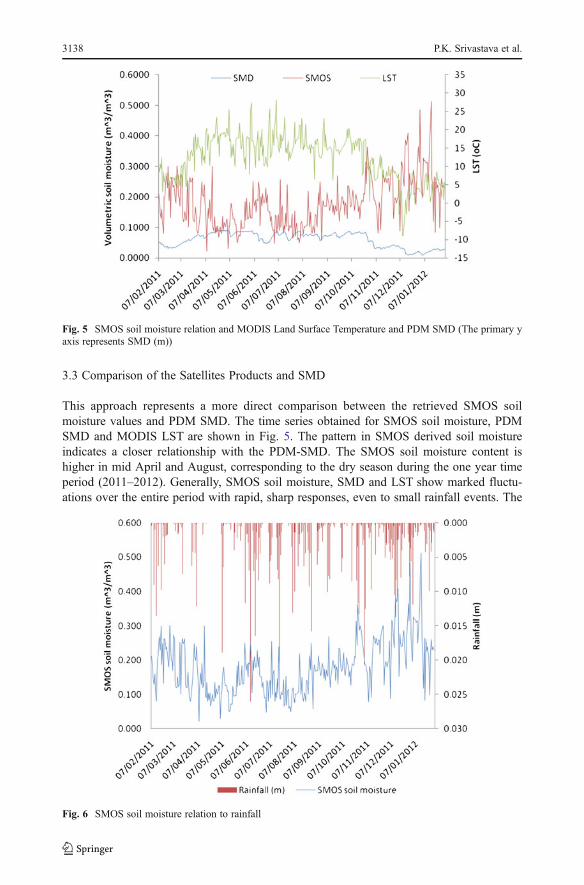
3.3 Comparison of the Satellites Products and SMD

This approach represents a more direct comparison between the retrieved SMOS soilmoisture values and PDM SMD. The time series obtained for SMOS soil moisture, PDMSMD and MODIS LST are shown in Fig. 5. The pattern in SMOS derived soil moistureindicates a closer relationship with the PDM-SMD. The SMOS soil moisture content ishigher in mid April and August, corresponding to the dry season during the one year timeperiod (2011–2012). Generally, SMOS soil moisture, SMD and LST show marked fluctu-ations over the entire period with rapid, sharp responses, even to small rainfall events. The

Fig. 5 SMOS soil moisture relation and MODIS Land Surface Temperature and PDM SMD (The primary yaxis represents SMD (m))

Fig. 6 SMOS soil moisture relation to rainfall

3138 P.K. Srivastava et al.

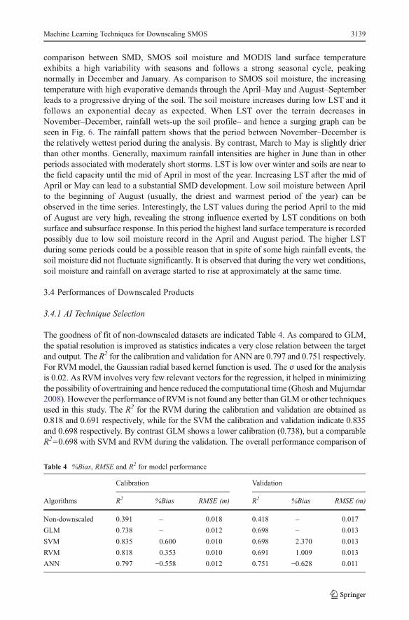
comparison between SMD, SMOS soil moisture and MODIS land surface temperatureexhibits a high variability with seasons and follows a strong seasonal cycle, peakingnormally in December and January. As comparison to SMOS soil moisture, the increasingtemperature with high evaporative demands through the April–May and August–Septemberleads to a progressive drying of the soil. The soil moisture increases during low LST and itfollows an exponential decay as expected. When LST over the terrain decreases inNovember–December, rainfall wets-up the soil profile– and hence a surging graph can beseen in Fig. 6. The rainfall pattern shows that the period between November–December isthe relatively wettest period during the analysis. By contrast, March to May is slightly drierthan other months. Generally, maximum rainfall intensities are higher in June than in otherperiods associated with moderately short storms. LST is low over winter and soils are near tothe field capacity until the mid of April in most of the year. Increasing LST after the mid ofApril or May can lead to a substantial SMD development. Low soil moisture between Aprilto the beginning of August (usually, the driest and warmest period of the year) can beobserved in the time series. Interestingly, the LST values during the period April to the midof August are very high, revealing the strong influence exerted by LST conditions on bothsurface and subsurface response. In this period the highest land surface temperature is recordedpossibly due to low soil moisture record in the April and August period. The higher LSTduring some periods could be a possible reason that in spite of some high rainfall events, thesoil moisture did not fluctuate significantly. It is observed that during the very wet conditions,soil moisture and rainfall on average started to rise at approximately at the same time.

3.4 Performances of Downscaled Products

3.4.1 AI Technique Selection

The goodness of fit of non-downscaled datasets are indicated Table 4. As compared to GLM,the spatial resolution is improved as statistics indicates a very close relation between the targetand output. The R2 for the calibration and validation for ANN are 0.797 and 0.751 respectively.For RVMmodel, the Gaussian radial based kernel function is used. The σ used for the analysisis 0.02. As RVM involves very few relevant vectors for the regression, it helped in minimizingthe possibility of overtraining and hence reduced the computational time (Ghosh andMujumdar2008). However the performance of RVM is not found any better than GLM or other techniquesused in this study. The R2 for the RVM during the calibration and validation are obtained as0.818 and 0.691 respectively, while for the SVM the calibration and validation indicate 0.835and 0.698 respectively. By contrast GLM shows a lower calibration (0.738), but a comparableR2=0.698 with SVM and RVM during the validation. The overall performance comparison of

Table 4 %Bias, RMSE and R2 for model performance

Calibration Validation

Algorithms R2 %Bias RMSE (m) R2 %Bias RMSE (m)

Non-downscaled 0.391 – 0.018 0.418 – 0.017

GLM 0.738 – 0.012 0.698 – 0.013

SVM 0.835 0.600 0.010 0.698 2.370 0.013

RVM 0.818 0.353 0.010 0.691 1.009 0.013

ANN 0.797 −0.558 0.012 0.751 −0.628 0.011

Machine Learning Techniques for Downscaling SMOS 3139

non-downscaled datasets with the GLM and other AI algorithms reveals that all techniques caneffectively downscale the SMOS soil moisture. It is evident from Table 4 that the ANN is moreefficient and highly skilful in downscaling the variability in the SMOS derived soil moisture.The overall observation indicates a low RMSE for ANN, imposing that the downscalingsubstantially improves the SMOS soil moisture. The SVM and RVM indicates a very high%Bias and comparable RMSE to GLM. The higher values of%Bias give an indication that it ismore sensitive to the significant over-prediction than the other schemes. The analysis of thedistribution of the %Bias and RMSE shows that the SMOS soil moisture is effectivelydownscaled with ANN techniques with low bias and RMSE. The overall performance ofGLM, ANN and RVM for SMOS downscaling shows that the downscaling of ANN are moreeffective than RVM (a probabilistic based approach) or kernel based algorithms like SVM. Thevalue of the%Bias and R2 are shown in Table 4. However, the main limitation with ANN is thatit takes more computational time than SVM or RVM. The application of GLM showscomparable performance and can be an alternative for downscaling in absence of AI techniques,as it is more basic and easy to implement.

3.4.2 Season Based Downscaling

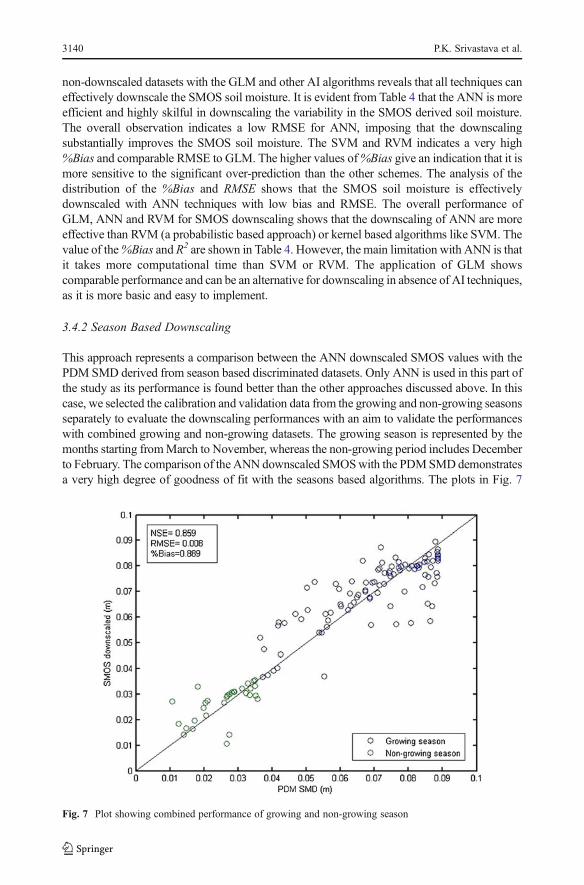
This approach represents a comparison between the ANN downscaled SMOS values with thePDM SMD derived from season based discriminated datasets. Only ANN is used in this part ofthe study as its performance is found better than the other approaches discussed above. In thiscase, we selected the calibration and validation data from the growing and non-growing seasonsseparately to evaluate the downscaling performances with an aim to validate the performanceswith combined growing and non-growing datasets. The growing season is represented by themonths starting fromMarch to November, whereas the non-growing period includes Decemberto February. The comparison of the ANN downscaled SMOSwith the PDMSMDdemonstratesa very high degree of goodness of fit with the seasons based algorithms. The plots in Fig. 7

Fig. 7 Plot showing combined performance of growing and non-growing season

3140 P.K. Srivastava et al.

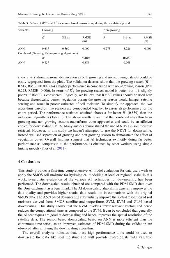
show a very strong seasonal demarcation as both growing and non-growing datasets could beeasily segregated from the plots. The validation datasets show that the growing season (R2=0.617, RMSE=0.009) has a higher performance in comparison with non-growing season (R2=0.273, RMSE=0.006). In terms of R2, the growing season model is better, but it is slightlypoorer if RMSE is considered. Logically, we believe that RMSE values should be used herebecause theoretically, denser vegetation during the growing season would hamper satellitesensing and result in poorer estimates of soil moisture. To simplify the approach, the twoalgorithms based on two seasons are compounded together to assess its performance for theentire period. The performance statistics obtained shows a far better R2 (0.859) than theindividual algorithms (Table 5). The above results reveal that the combined algorithm fromgrowing and non-growing seasons outperforms other approaches and could be an efficientchoice for downscaling SMOS. Many authors demonstrated the use of NDVI in soil moistureretrieval. However, in this study we haven’t attempted to use the NDVI for downscaling,instead we used separation of growing and non growing season to demonstrate the effect ofvegetation cover. Overall findings suggest that AI techniques explicitly doing far betterperformance as comparison to the performance as obtained by other workers using simplelinking models (Piles et al. 2011).

4 Conclusions

This study provides a first-time comprehensive AI model evaluation for data users wish toapply the SMOS soil moisture for hydrological modelling at local or regional scale. In thiswork, synergistic evaluation of the various AI techniques for downscaling has beenperformed. The downscaled results obtained are compared with the PDM SMD data overthe Brue catchment as a benchmark. The AI downscaling algorithms generally improves thedata quality and provides higher spatial data resolution in comparison with the originalSMOS data. The ANN based downscaling substantially improve the spatial resolution of soilmoisture derived from SMOS satellite and outperforms SVM, RVM and GLM baseddownscaling. This study shows that the RVM involves fewer relevant vectors and hencereduces the computational time as compared to the SVM. It can be concluded that generallythe AI techniques are good at downscaling and hence improves the spatial resolution of thesatellite data. The season based downscaling based on ANN is more efficient than thecontinuous time series, as an improved estimates of PDM SMD during the validation areobserved after applying the downscaling algorithm.

The overall analysis indicates that, these high performance tools could be used todownscale the data like soil moisture and will provide hydrologists with valuable

Table 5 %Bias, RMSE and R2 for season based downscaling during the validation period

Variables Growing Non-growing

R2 %Bias RMSE(m)

R2 %Bias RMSE(m)

ANN 0.617 0.560 0.009 0.273 3.726 0.006

Combined (Growing +Non-growing algorithms)

R2 %Bias RMSE

ANN 0.859 0.889 0.008

Machine Learning Techniques for Downscaling SMOS 3141

information on applicability of SMOS for SMD estimations. Further exploration of thispotentially valuable data source by the scientific community should be encouraged so thatuseful understanding and knowledge could be accumulated in the technical literaturedomain. Future research should also focus on the application of the above mentioned schemefor hydrological forecasting integrated with uncertainty analysis.

Acknowledgments The authors would like to thank the Commonwealth Scholarship Commission, BritishCouncil, United Kingdom and Ministry of Human Resource Development, Government of India for providingthe necessary support and funding for this research. The authors are highly thankful to the European SpaceAgency for providing the SMOS data. The authors would like to acknowledge the British Atmospheric DataCentre, United Kingdom for providing the ground observation datasets. The authors also acknowledge theAdvanced Computing Research Centre at University of Bristol for providing the access to supercomputerfacility (The Blue Crystal).

References

Al-Shrafany D, Rico-Ramirez M, Han D (2012a) Calibration of roughness parameters using rainfall runoffwater balance for satellite soil moisture retrieval. J Hydrol Eng 17:704–714. doi:10.1061/(ASCE)HE.1943-5584.0000508

Al-Shrafany D, Rico-Ramirez M, Han D, Bray M (2012b) Comparative assessment of soil moisture estima-tion from land surface model and satellite remote sensing based on catchment water balance. Met Apps.doi:10.1002/met.1357

Anderson JA, Davis J (1995) An introduction to neural networks, vol 1. MIT Press, Cambridge, MABishop CM, Tipping ME (2000) Variational relevance vector machines. Proceedings of the Sixteenth

conference on Uncertainty in artificial intelligence. Morgan Kaufmann Publishers IncCaputo B, Sim K, Furesjo F, Smola A (2002) Appearance-based Object Recognition using SVMs: which

Kernel Should I Use?. In Proc of NIPS workshop on Statistical methods for computational experiments invisual processing and computer vision, Whistler (Vol. 2002)

Carlson T (2007) An overview of the“ triangle method” for estimating surface evapotranspiration and soilmoisture from satellite imagery. Sensors 7(8):1612–1629

Foody G (2008) RVM–based multi–class classification of remotely sensed data. Int J Remote Sens29(6):1817–1823

Gao J (2008) Digital analysis of remotely sensed imagery. McGraw-Hill ProfessionalGhosh S, Mujumdar P (2008) Statistical downscaling of GCM simulations to streamflow using relevance

vector machine. Adv Water Resour 31(1):132–146Goward SN, Xue Y, Czajkowski KP (2002) Evaluating land surface moisture conditions from the remotely

sensed temperature/vegetation index measurements: an exploration with the simplified simple biospheremodel. Remote Sens Environ 79(2):225–242

Han D, Cluckie I (2004) Support vector machines identification for runoff modeling. In: pp 21–24Han D, Yang Z (2001) River flow modelling using support vector machines. In: pp 494–499Han D, Kwong T, Li S (2007) Uncertainties in real–time flood forecasting with neural networks. Hydrol

Process 21(2):223–228Ishak A, Remesan R, Srivastava P, Islam T, Han D (2013) Error correction modelling of wind speed through

hydro-meteorological parameters and mesoscale model: a hybrid approach. Water Resour Manag27(1):1–23. doi:10.1007/s11269-012-0130-1

Islam T, Rico-Ramirez MA, Han D, Srivastava PK (2012) Artificial intelligence techniques for clutteridentification with polarimetric radar signatures. Atmos Res 109–110:95–113. doi:10.1016/j.atmosres.2012.02.007

Jackson TJ (1993) III. Measuring surface soil moisture using passive microwave remote sensing. HydrolProcess 7(2):139–152

Johnson RA, Wichern DW (2002) Applied multivariate statistical analysis, vol 4. Prentice Hall, Upper SaddleRiver

Karatzoglou A, Smola A, Hornik K, Zeileis A (2005) Kernlab–kernel methods. R package, Version 0.6-2.http://epub.wu.ac.at/1048/

3142 P.K. Srivastava et al.

Kerr YH,Waldteufel P,Wigneron JP, Martinuzzi J, Font J, Berger M (2001) Soil moisture retrieval from space: theSoil Moisture and Ocean Salinity (SMOS) mission. IEEE Trans Geosci Rem Sens 39(8):1729–1735

Kerr Y, Waldteufel P, Richaume P, Davenport I, Ferrazzoli P, Wigneron J (2006) SMOS level 2 processor soilmoisture algorithm theoretical basis document (ATBD). SM-ESL (CBSA), CESBIO, Toulouse, SO-TN-ESL-SM-GS-0001, V5 a, 15/03

Kerr YH,Waldteufel P, Richaume P,Wigneron JP, Ferrazzoli P,Mahmoodi A, Al Bitar A, Cabot F, Gruhier C, JugleaSE (2012) The SMOS soil moisture retrieval algorithm. IEEE Trans Geosci Rem Sens 50(5):1384–1403

Legates DR, Mahmood R, Levia DF, DeLiberty TL, Quiring SM, Houser C, Nelson FE (2011) Soil moisture:a central and unifying theme in physical geography. Prog Phys Geogr 35(1):65–86

Lindsey JK (1997) Applying generalized linear models. Springer Verlag, New YorkLiu J, Han D (2010) Indices for calibration data selection of the rainfall-runoff model. Water Resour Res

46(4):W04512Mallick K, Bhattacharya BK, Patel N (2009) Estimating volumetric surface moisture content for cropped soils

using a soil wetness index based on surface temperature and NDVI. Agric For Meteorol 149(8):1327–1342McCullagh P, Nelder JA (1989) Generalized linear models. Chapman & Hall/CRCMerlin O, Walker JP, Chehbouni A, Kerr Y (2008) Towards deterministic downscaling of SMOS soil moisture

using MODIS derived soil evaporative efficiency. Remote Sens Environ 112(10):3935–3946Mladenova I, Lakshmi V, Jackson TJ, Walker JP, Merlin O, de Jeu RAM (2011) Validation of AMSR-E soil

moisture using L-band airborne radiometer data from National Airborne Field Experiment 2006. RemSens Environ 115(8):2096–2103

Moody J, Hanson S, Krogh A, Hertz JA (1995) A simple weight decay can improve generalization. AdvNeural Inform Process Syst 4:950–957

Moore R (2007) The PDM rainfall-runoff model. Hydrol Earth Syst Sci 11(1):483–499Panciera R, Walker JP, Kalma JD, Kim EJ, Hacker JM, Merlin O, Berger M, Skou N (2008) The NAFE’05/

CoSMOS data set: toward SMOS soil moisture retrieval, downscaling, and assimilation. IEEE TransGeosci Rem Sens 46(3):736–745

Piles M, Camps A, Vall-Llossera M, Corbella I, Panciera R, Rudiger C, Kerr YH, Walker J (2011)Downscaling SMOS-derived soil moisture using MODIS visible/infrared data. IEEE Trans Geosci RemSens 49(9):3156–3166

Pinori S, Crapolicchio R, Mecklenburg S (2008) Preparing the ESA-SMOS (Soil Moisture and OceanSalinity) mission-Overview of the user data products and data distribution strategy. Microwave Radiom-etry and Remote Sensing of the Environment, 2008. MICRORAD 2008. IEEE

RDevelopment C (2010) TEAM. 2006. R: a language and environment for statistical computing. R Founda-tion for Statistical Computing, Vienna, Austria. ISBN 3-900051-07-0, URL http://www.R-project.org

Remesan R, Shamim MA, Han D, Mathew J (2009) Runoff prediction using an integrated hybrid modellingscheme. J Hydrol 372(1–4):48–60

Ridler ME, Sandholt I, Butts M, Lerer S, Mougin E, Timouk F, Kergoat L, Madsen H (2012) Calibrating asoil–vegetation–atmosphere transfer model with remote sensing estimates of surface temperature and soilsurface moisture in a semi arid environment. J Hydrol 436–437:1–12

Ripley B (2009) Feed-forward neural networks and multinomial log-linear models. R-packageSandholt I, Rasmussen K, Andersen J (2002) A simple interpretation of the surface temperature/vegetation

index space for assessment of surface moisture status. Remote Sens Environ 79(2):213–224Schoof JT, Pryor S (2001) Downscaling temperature and precipitation: a comparison of regression–based

methods and artificial neural networks. Int J Climatol 21(7):773–790Sivapragasam C, Muttil N (2005) Discharge rating curve extension–a new approach. Water Resour Manag

19(5):505–520Srivastava PK, Han D, Rico-Ramirez MA (2012a) Assessment of SMOS satellite derived soil moisture for soil

moisture deficit stimation. Symposium on Prediction in Ungauged basin (PUBS) co-organized by DelftUniversity of Technology, Delft, Netherlands and International Association of Hydrological Sciences(IAHS) dated 22–25 October 2012:1

Srivastava PK, Han D, Rico-Ramirez MA, Bray M, Islam T (2012b) Selection of classification techniques forland use/land cover change investigation. Adv Space Res 50(9):1250–1265. doi:10.1016/j.asr.2012.06.032

Srivastava PK, Han D, Rico-Ramirez MA (2013a) Data fusion techniques for an improved soil moistureretrieval using SMOS and WRF-NOAH Land surface model SMOS land application workshop, ESA-ESRIN, Frascati, Italy 25–27 February 2013

Srivastava PK, Han D, Rico-Ramirez MA, Islam T (2013b) Comparative assessment of evapotranspirationderived from NCEP and ECMWF global datasets through Weather Research and Forecasting model.Atmos Sci Lett. doi:10.1002/asl.427

Machine Learning Techniques for Downscaling SMOS 3143

Thakur J, Srivastava PK, Singh SK, Vekerdy Z (2012) Ecological monitoring of wetlands in semi-arid regionof Konya closed Basin, Turkey. Reg Environ Chang 12(1):133–144. doi:10.1007/s10113-011-0241-x

Tipping ME (2001) Sparse Bayesian learning and the relevance vector machine. J Mach Learn Res 1:211–244Trigo RM, Palutikof JP (2001) Precipitation scenarios over Iberia: a comparison between direct GCM output

and different downscaling techniques. J Clim 14(23):4422–4446Vapnik V, Golowich SE, Smola A (1997) Support vector method for function approximation, regression

estimation, and signal processing. Adv Neural Inform Process Syst 9:281–287Wagner W, Naeimi V, Scipal K, de Jeu R, Martínez-Fernández J (2007) Soil moisture from operational

meteorological satellites. Hydrogeol J 15(1):121–131Wan Z (1999) MODIS land-surface temperature algorithm theoretical basis document (LST ATBD). Institute

for Computational Earth System Science, Santa Barbara, 75Wang YM, Traore S, Kerh T, Leu JM (2011) Modelling reference evapotranspiration using feed forward

backpropagation algorithm in arid regions of Africa. Irrig Drain 60(3):404–417Weichert A, Bürger G (1998) Linear versus nonlinear techniques in downscaling. Clim Res 10:83–93Wu C, Chau K (2011) Rainfall-runoff modeling using artificial neural network coupled with singular spectrum

analysis. J Hydrol 399(3):394–409Zhang Y, Ding X, Liu Y, Griffin P (1996) An artificial neural network approach to transformer fault diagnosis.

IEEE Trans Power Deliv 11(4):1836–1841Zhang G, Patuwo BE, Hu MY (1998) Forecasting with artificial neural networks: the state of the art. Int J

Forecast 14(1):35–62

3144 P.K. Srivastava et al.