7038 IEEE TRANSACTIONS ON GEOSCIENCE AND REMOTE SENSING, VOL. 52, NO. 11, NOVEMBER 2014

A Kurtosis-Based Approach to Detect RFI in SMOSImage Reconstruction Data Processor

Ali Khazâal, François Cabot, Eric Anterrieu, Member, IEEE, and Yan Soldo

Abstract—The Soil Moisture and Ocean Salinity (SMOS) mis-sion is a European Space Agency project aimed to observe twoimportant geophysical variables, i.e., soil moisture over land andocean salinity by L-band microwave imaging radiometry. Thiswork is concerned with the contamination of the SMOS data byradio-frequency interferences (RFIs), which degrades the perfor-mance of the mission. In this paper, we propose an approach thatdetects if a given snapshot is contaminated, or not, by RFI. Thisapproach is based on evaluating the kurtosis of each snapshot ordata set, using all interferometric measurements provided by theinstrument. The obtained kurtosis is considered as an indicator onhow much the snapshot is polluted by RFI, thus allowing the userto decide on whether to keep or discard it.

Index Terms—Kurtosis, radio-frequency interference (RFI),radiometry, remote sensing, synthetic aperture imaging.

I. INTRODUCTION

THE Soil Moisture and Ocean Salinity (SMOS) mission is aEuropean Space Agency’s (ESA) Earth Explorer Mission,

which was launched on November 2, 2009 and aimed to retrieveglobal measurements of soil moisture (SM) and ocean salinity(OS) [1]. These two parameters are key variables used inpredictive hydrological, oceanographic, and atmospheric mod-els [2], [3]. The instrument used onboard SMOS is the first2-D spaceborne Microwave Imaging Radiometer with ApertureSynthesis (MIRAS), which operates in the passive L-band [4].

The contamination of the SMOS measurements by radio-frequency interferences (RFIs) has been studied and consideredbefore the launch of the instrument, although it is operatingin the protected L-band [5]. However, many RFI sources weredetected during the commissioning phase in different regionsaround the world, thus degrading the quality of SMOS retrievals[6]. The observed RFI are mainly due to man-made emissionsfalling within the protected band. These emissions are either il-legal emissions inside the protected band or excessive unwantedemissions from systems operating in the adjacent bands.

The presence of RFI in the SMOS data has been widelyaddressed since the launch of the instrument. Many studies

Manuscript received May 6, 2013; revised July 29, 2013 and November 15,2013; accepted February 11, 2014. Date of publication March 5, 2014.

A. Khazâal, F. Cabot, and Y. Soldo are with the Center for the Study of theBIOsphere (CESBIO), Universitè de Toulouse, CNRS, CNES & IRD, 31401Toulouse, France (e-mail: ali.khazaal@cesbio.cnes.fr; francois.cabot@cesbio.cnes.fr; yan.soldo@cesbio.cnes.fr).

E. Anterrieu is with the Research Institute of Astrophysics and Planetology,Observatoire Midi-Pyrénées, 31400 Toulouse, France (e-mail: eric.anterrieu@irap.omp.eu).

Color versions of one or more of the figures in this paper are available onlineat http://ieeexplore.ieee.org.

Digital Object Identifier 10.1109/TGRS.2014.2306713

have been conducted in order to detect and localize the RFIsources and mitigate them if possible [8], [9]. This paper isonly concerned with the detection part. The results presentedhere are also compared to those obtained with the zero-baselinevisibility detection approach, which was proposed recently [7],and to be implemented in the SMOS image reconstruction dataprocessor. Here, we propose a kurtosis-based approach, usingall SMOS interferometric measurements or visibilities, to detectif a given snapshot is contaminated by RFI and also the degreeof this contamination.

The level-1 (L1) processor prototype in SMOS Data Process-ing Ground Segment (DPGS) is a software processing chainthat will convert all satellite data from raw products (level-0data) into geolocated brightness temperatures at different obser-vation angles (L1c data) through two more intermediate prod-ucts: calibrated visibilities or interferometric measurements(L1a data) and brightness-temperature Fourier components(L1b data) [10]. The RFI detection approach proposed hereafteris a snapshot-based method performed alongside the imagereconstruction procedure. It uses the interferometric measure-ments of each snapshot and transforms them into the spatialdomain before evaluating a kurtosis value to detect whether thesnapshot is contaminated by RFI, as well as the degree of thiscontamination.

The presence of RFI in the different L1 products is shown inSection II. The notion of kurtosis is introduced in Section III,as well as an explanation about its relationship with RFI. InSection IV, we propose an approach that extends the notion ofkurtosis to the case of SMOS. Finally, Section V is devotedto illustrate the performance of the proposed approach andcomparing it with the zero-baseline approach using L1a dataacquired from the SMOS DPGS.

II. RFI IN SMOS L1 DATA

The SMOS L1 processor is responsible for the reconstruc-tion of the brightness-temperature maps from the satellitedata. At first, it converts the calibrated visibilities (L1a data)into brightness-temperature Fourier components (L1b data)[10]. Then, the Fourier components are used to calculatethe brightness-temperature values (L1c data) anywhere in thespatial domain, by simply applying an inverse fast Fouriertransform to the retrieved L1b data.

Regarding the retrieval of SM and OS (level 2), they areobtained separately using L1c data (when processing an L1bproduct, we obtain two L1c products: one over land used in theretrieval of SM and the other over ocean used in the retrieval ofOS). As a consequence, RFI contamination in lower levels will

0196-2892 © 2014 IEEE. Personal use is permitted, but republication/redistribution requires IEEE permission.See http://www.ieee.org/publications_standards/publications/rights/index.html for more information.

KHAZÂAL et al.: KURTOSIS APPROACH TO DETECT RFI IN SMOS IMAGE RECONSTRUCTION DATA PROCESSOR 7039

Fig. 1. (Top) Variation of the average of the zero-baseline visibilities V (0)for an L1a orbit on July 11, 2010, in both (blue) X- and (red) Y -polarizations.(Bottom) Variation of the zero-frequency Fourier components T̂ (0) obtainedfrom its corresponding L1b orbit.

propagate, if not corrected or filtered, to higher levels and, insome cases, may prevent the retrieval of SM and OS [6].

The presence of RFI in L1 data products can be observedeasily. For L1a and L1b data, it can be seen respectively bysimply plotting the temporal variation of the visibilities or theFourier components for a specified baseline or spatial frequency(preferably the zero baseline/frequency associated to the au-tocorrelation of the three Noise Injection Radiometers (NIRs)of MIRAS since the signal-to-noise ratio (SNR) is inverselyproportional to the magnitude of the baseline/frequency [11],[12]). On the other hand, for L1c data, it can be seen in asnapshot basis by looking directly to the retrieved brightness-temperature maps.

To illustrate the presence of RFI in L1 data, we considerthe following descending orbit taken on July 11, 2010, whichpasses over the Arctic Ocean, Russia, the Middle East, theMediterranean Sea, Africa, the Southern Ocean, and Antarctica.For the corresponding L1a product, we show in Fig. 1 the tem-poral variation of the average of the zero-baseline visibilitiesacquired by the three NIRs. As shown in [7], these variationsshould be quite smooth, while here, a strange behavior can benoticed, far from smooth and reminds that of outliers, as weobserve between 15 h:51 m and 16 h:05 m.

The same behavior can be seen at the same time using thecorresponding L1b product, as also shown in Fig. 1, by plottingthe temporal variation of the zero-frequency Fourier compo-nents. This is quite natural since the relationship between thecalibrated visibilities and the brightness temperature is linear[13], [14].

For the L1c data, Fig. 2 shows the retrieved maps for twoconsecutive snapshots over Egypt in X- and Y -polarizations,respectively. At first, we should indicate that SMOS data atthe instrument level (X- and Y -polarizations) are linear com-binations of those at the earth level (H and V polarizations), asdemonstrated in [15] and [16]. Furthermore, the field of view(FOV) of MIRAS is the entire half-space in front of the instru-ment, which has the form of a unit circle in the antenna plane.However, because of the large spacing between the antennas of

Fig. 2. Example of presence of RFI sources in L1c data sets: retrievedbrightness temperature maps of two snapshots inside the EAFFOV in (left) X-and (right) Y -polarizations. The snapshots are taken from an orbit on July 11,2010 and showed for two different color scales: (bottom) real scale and (top)scale between 0 and 350 K.

MIRAS, the reconstructed FOV is a 2-D hexagon inside the unitcircle and subject to earth and sky aliasing [17]. Consequently,the reconstruction is only restricted to an Extended Alias-FreeFOV (EAFFOV) [2], where only sky aliasing is allowed sinceit can be corrected.

Back now to Fig. 2, we can distinguish many RFI sourceswith a brightness temperature up to 13 000 K. The effect ofeach source on the reconstruction is not necessarily local andimportant sidelobes appear in the retrieved maps and can bereferred as the tails of the RFI sources. We should also indicatethat, inside the wide FOV of MIRAS (unit circle), any RFIsource can be located in three different zones.

1) Inside the EAFFOV: the retrieved L1c brightness-temperature maps are here affected by the source itselfand its tails.

2) Outside the EAFFOV but inside the 2-D hexagon: TheL1c retrieved maps are here affected only by the tails ofthe source. The degree of contamination depends, in thiscase, on the intensity of the source.

3) Outside the 2-D hexagon: although the source is outsidethe reconstructed FOV (hexagon), one or two of its aliasesare inside the discarded aliased regions. Consequently,the retrieved L1c maps are affected by their tails.

III. KURTOSIS AND RFI

Kurtosis is a statistical measure used to describe the distri-bution of observed data around its mean. It is used generally tomeasure the degree of peakedness or flatness in a distribution.A high kurtosis portrays a distribution with important peaksand large tails, whereas a low kurtosis portrays a distribution

7040 IEEE TRANSACTIONS ON GEOSCIENCE AND REMOTE SENSING, VOL. 52, NO. 11, NOVEMBER 2014

Fig. 3. Density of probability ρ(P ) of a normal distribution or mesokurtic(kurtosis = 0), a leptokurtic distribution (positive kurtosis), and a platykurticdistribution (negative kurtosis).

mostly concentrated toward the mean. The kurtosis is a bettermeasure of the degree of heterogeneity than the variance; itgives more weight to the pixels, which contribute to the obviousheterogeneity in an image, as for outliers, or in our case, RFI.

According to [18], the kurtosis of a distribution P can bedefined as the fourth moment around the mean divided by thesquare of the variance of the probability distribution

K =E(P − μ)4

(E(P − μ)2)2=

μ4

σ4(1)

where μ is the mean, μ4 is the fourth moment around the mean,and σ is the standard deviation.

A normal distribution has a kurtosis of 3; thus, we oftenuse an excess of kurtosis K − 3, so that the reference normaldistribution has a kurtosis of zero. In this case, (1) becomes

K =E(P − μ)4

(E(P − μ)2)2− 3 =

μ4

σ4− 3. (2)

Given the last definition of kurtosis [see (2)], it has beenshowed in [18] and [19] and illustrated in Fig. 3 that

• Distributions with positive kurtosis or leptokurtic haveheavier tails and/or higher peaks than normal distributionsor mesokurtic (kurtosis equal to zero).

• Distributions with negative kurtosis or platykurtic havelighter tails and are flatter.

In the next section, an RFI detection approach based onevaluating the kurtosis of each data set is proposed using SMOSL1a data. For this approach, a negative kurtosis indicates thatthe data set in question is free from RFI contamination, whereasa positive kurtosis means that it is contaminated by RFI eitherbecause one or more sources are present or because of thepresence of heavy tails.

IV. RFI DETECTION APPROACH

Data degradation due to RFI is a major issue for SMOS users.The corrupted data need to be identified, corrected if possible,or discarded if not, before the level-2 product is delivered. Untilnow, there is no efficient approach to mitigate the contributionof RFI from SMOS data at any level. Therefore, efficient RFIdetection approaches are mostly needed to flag the contami-nated snapshots and allow the user to filter properly the databefore retrieving SM and OS.

Recently, a detection approach has been proposed that usesthe zero-baseline visibilities provided by the three reference

radiometers of SMOS (NIRs) [7]. A limitation of this approachis that spatially localized sources will have much lower signalamplitude in the visibility domain than in the spatial domainbecause a zero-baseline visibility describes the average bright-ness temperature of the overall observed scene [8]. Anotherlimitation is the saturation of the NIRs’ measurements forvery high and continuous RFI levels. Hereafter, we propose adifferent detection approach that uses all L1a measurements orvisibilities.

In fact, the image reconstruction processor takes the in-terferometric measurements and retrieves the correspondentbrightness-temperature Fourier components using a band-limited reconstruction approach [14]. Before the reconstruction,the interferometric measurements are corrected from contribu-tions coming from different foreign sources such as the sun, themoon, the sun glint, and the sky [10]. This approach should beapplied on the corrected visibilities V just before applying theimage reconstruction procedure and is defined as follows:

• Step 1: The visibilities V are defined in the Fourierdomain and are confined to a limited star-shaped windowover a hexagonally sampled grid (u, v) [4]. The first stepis to calculate I the inverse fast Fourier transform of Vover a spatial grid (ξ,η), which is the dual grid of (u, v).This grid (ξ, η) is defined over the 2-D hexagonal FOV ofMIRAS. That is

I(ξ, η) = T F−1ξ,η [V (u, v)] .

• Step 2: As mentioned earlier, we have aliased regions inthe 2-D hexagonal FOV of MIRAS due to the large spac-ing between the antennas. Therefore, the kurtosis, which isa statistical measure, cannot be calculated over the entirehexagon because of the contribution of the aliased regions.The solution is to discard, from I, all values outside theEAFFOV, as follows:

I = I(ξEAFFOV, ηEAFFOV).

• Step 3: Calculate, for each snapshot, a land/ocean maskinside the EAFFOV, and separate I into IL and IO, asfollows:

IL = I(ML == 1)

IO = I(MO == 1)

where ML and MO are two binary masks defined respec-tively over land and ocean, as follows:

ML =1 for Land pixels and 0 otherwiseMO =1 for Ocean pixels and 0 otherwise.

• Step 4: Using (2), calculate separately the kurtosis overland (KL) and ocean (KO).

• Step 5: If KL or KO have positive values, the snapshotin question is contaminated by RFI either because of thepresence of RFI sources in the EAFFOV or because ofthe presence of high tails/sidelobes due to sources outsidethe EAFFOV.

One question arises here. Why do we separate the land regionfrom the ocean region and calculate the kurtosis for each region

KHAZÂAL et al.: KURTOSIS APPROACH TO DETECT RFI IN SMOS IMAGE RECONSTRUCTION DATA PROCESSOR 7041

separately? In fact, when we calculate the inverse fast Fouriertransform of V , the contrast over land pixels of I is muchhigher than the contrast over ocean pixels. Consequently, thekurtosis, if calculated over both regions, may have positivevalues leading to many false alarms. As a solution, we proposeto separate land from ocean and calculate the kurtosis for eachregion. Taking also into consideration the Gibbs oscillationsnear the coasts, we consider that all ocean pixels within a40-km range from the coast are considered as land (using theMERIS uncertainty map for ESA’s mission ENVISAT withits coasts extended to 40 km [20]). We should also indicatethat inside the EAFFOV, we have a limited number of pixels(about 7000 pixels are inside the EAFFOV using the hexagonalgrids of MIRAS [14]). To minimize the uncertainty error thatmay arise from land or ocean regions with a small number ofpixels, we only calculate both kurtosis over land and ocean ifthe corresponding area is at least 20% of the overall surface.Otherwise, only one region is considered, and only one kurtosisvalue is obtained.

Another important question can be asked here. Can weconsider the zero kurtosis as a valid threshold even if thedistribution I is not Gaussian? It is essential to precise that, inour case, clean snapshots will not have a zero kurtosis sincethe distribution is not Gaussian. However, all results obtainedusing SMOS L1a measurements (see Section V) have shownthat clean snapshots always have a negative kurtosis, whereascontaminated snapshots have a positive kurtosis, which is anincreasing function of the intensity of RFI contamination. Weshould also indicate that a negative kurtosis does not meanthat the snapshot in question is flat, but it reflects the absenceof peakedness or heavy tails or, in our case, a snapshot freefrom RFI contamination. For those clean data sets, the varia-tion of kurtosis is smooth with values closer to −1 for morehomogeneous scenes and closer to zero for less homogeneousor heterogeneous scenes. As for contaminated snapshots, wehave found that the degree of contamination is an increasingfunction with the value of the kurtosis. Finally, to limit evenmore the number of false alarms, it has been proposed in [21]to calculate a standard error of kurtosis (SEK) and suppose thatdistributions with kurtosis higher than 2SEK are considered asleptokurtic. Many formulas have been given for SEK, but herewe consider a rough approximation given by [21] and defined as

SEK =√

24/n (3)

where n is the number of samples (here pixels) used tocalculate the kurtosis. In our case, n is equal to the number ofland or ocean pixels for each distribution.

V. RESULTS

The results presented hereafter are obtained using L1a datataken from the SMOS DPGS. The kurtosis detection approachis tested in the following cases.

• Using clean L1a data: to study its robustness versus falsealarms of presence of RFI. The results are compared tothose obtained using the zero-baseline visibility detectionapproach.

Fig. 4. Variation of the kurtosis KO over the Pacific Ocean for 300 snapshotsin each polarization [(top) X and (bottom) Y ] taken on January 28, 2011. Here,no data sets are detected as contaminated by RFI.

Fig. 5. Average brightness temperatures acquired by the three NIRs for 300data sets in each polarization [(top) X and (bottom) Y ] taken on January28, 2011, over the Pacific Ocean. The green dots correspond to snapshotscontaminated by RFI, as detected by the zero-baseline approach (two falsealarms in X-polarization and one in Y -polarization).

• Using contaminated L1a data: to see its capacity to dis-tinguish between clean and contaminated snapshots. Acomparison is also proposed here with the zero-baselineapproach.

• Using a subset of L1a data contaminated by low RFIsignals to study the sensitivity of this approach versus lowsources, which are the most difficult to detect.

• Using three days of L1a data: the objective is to obtain aglobal coverage of the contaminated snapshots over landand ocean.

A. Clean L1a Data

The kurtosis approach is applied first over 300 clean andconsecutive data sets in each polarization X and Y taken froman L1a ascending orbit over the Pacific Ocean on January 28,2011. Shown now in Fig. 4 is the variation of the kurtosis overthe ocean KO (KL = 0 since the EAFFOV is 100% ocean),which seems very smooth and always negative (no false alarms)with a mean value around −0.6 in X-polarization and −1 inY -polarization. These results are to be compared with thoseobtained by the zero-baseline visibility approach shown inFig. 5 and indicating that two data sets in X-polarization andone data set in Y -polarization are contaminated by RFI (falsealarms).

7042 IEEE TRANSACTIONS ON GEOSCIENCE AND REMOTE SENSING, VOL. 52, NO. 11, NOVEMBER 2014

Fig. 6. Variation of the kurtosis KL over Australia for 150 snapshots ineach polarization [(top) X and (bottom) Y ] taken on July 4, 2011. Here, foursnapshots are detected as contaminated by RFI (in green) in X-polarization(false alarms) and none in Y -polarization.

Fig. 7. Average brightness temperatures acquired by the three NIRs for 150L1a data sets in each polarization [(top) X and (bottom) Y ] taken on July 4,2011, over Australia. The green dots correspond to snapshots contaminatedby RFI, as detected by the zero-baseline approach (only one false alarm inX-polarization).

The same test is repeated over land, where we now considerthe data sets of 300 clean and consecutive snapshots (150 ineach polarization X and Y ) of an ascending L1a orbit takenover Australia on July 4, 2011. The variation of kurtosis KL

shown in Fig. 6 is smooth to a certain extent, taking intoconsideration the heterogeneity of the observed scenes. Fourfalse alarms are detected here in X-polarization (1.3% of thetotal number of snapshots) with a kurtosis up to 0.05 comparedto one false alarm with the zero-baseline approach, as shownin Fig. 7.

Although both approaches have detected only few falsealarms, we should insist that the number of false alarms isexpected to be higher for several reasons.

• Since the distribution I in the spatial domain is not Gaus-sian, natural phenomenon may appear in I as peaks dueto the heterogeneity of the scenes and leads to positivekurtosis and false alarms of presence of RFI.

• When the Southern Ocean enters in the EAFFOV, an icelayer will appear, thus pushing the kurtosis to positivevalues (False alarms), as shown hereafter.

• If the sun if not corrected or not well corrected in theL1 data processor, the kurtosis value will be positive,particularly over the ocean.

Fig. 8. Variation of the kurtosis KL over land for the L1a orbit on July 11,2010 described in Section II in (top) X- and (bottom) Y -polarizations. Thegreen dots correspond to snapshots contaminated by RFI, whereas the red/bluedots correspond to clean snapshots.

Fig. 9. Variation of the kurtosis KO over the ocean for the L1a orbit on July11, 2010 described in Section II in (top) X- and (bottom) Y -polarizations. Thegreen dots correspond to snapshots contaminated by RFI, whereas the red/bluedots correspond to clean snapshots.

However, the separation of the land region from the oceanregion helps to reduce the number of false alarms, as well astaking into consideration the standard error of kurtosis. Overall,the number of false alarms remains low, and the expectedsmooth temporal variation of the kurtosis for clean data enablesus to identify most of these false alarms.

B. Contaminated L1a Data

Here, the RFI detection approach is applied on data con-taminated by RFI. Considering the L1a orbit of July 11, 2010,which was described earlier in Section II, Figs. 8 and 9 showthe variation of kurtosis over land (KL) and ocean (KO),respectively. From these results, we can deduce the following:

• Over the Arctic Ocean (East Siberian Sea), the data setsare contaminated by RFI in X-polarization but not inY -polarization. This is possible if the RFI sources arepolarized, as radar sources. On the other hand, a high-level RFI source in X-polarization may have some leakagein the Y -polarization. Therefore, the negative kurtosisobtained in Y -polarization can also reflect the difficultyof the kurtosis approach to detect very low levels of RFIcontamination. On the other hand, a further investigationhas shown that these sources correspond to active radar

KHAZÂAL et al.: KURTOSIS APPROACH TO DETECT RFI IN SMOS IMAGE RECONSTRUCTION DATA PROCESSOR 7043

Fig. 10. Projection map of the whole FOV of MIRAS (green) and theEAFFOV (blue) for a snapshot over the Arctic Ocean from the descending L1aorbit on July 11, 2010. In addition, the active radar sources of the DEW line(red) and the latitude and the longitude of earth surface point in the snapshot’sboresight direction (magenta) for the L1a orbit are shown in this figure.

stations from the Distant Early Warning Line (DEW line)located in the far northern Arctic region of Canada, withstations along the North Coast, Alaska, Greenland, andIceland. Fig. 10 shows a projection map of the FOV andthe EAFFOV of MIRAS for one of the contaminatedsnapshots over the Arctic Ocean, as well as the active radarsources of the DEW line. As we can notice, these sourcesare outside the EAFFOV, but they contribute to the L1ameasurements, thus producing heavy tails or sidelobes inthe retrieved maps.

• Over parts of Russia, the Middle East, and NorthernAfrica, most of the data are contaminated by RFI. Thekurtosis here reaches values near 1000 over land and 400over ocean, which describes the high intensity of RFI inthese regions. An example of RFI contamination over theMiddle East was shown earlier in Fig. 2.

• The situation improves from Central Africa to Antarcticawith almost no RFI sources. However, somewhere overthe ocean, around a latitude of −53◦ and a longitude of11◦, where the FOV is almost 100% ocean, the kurtosissuddenly becomes positive (up to 5 in X-polarization and1 in Y -polarization) for a certain number of snapshotsbefore returning to an almost stable negative value. Afurther investigation has showed that, at the precise mo-ment where KO becomes positive, the Southern Ocean (orthe Antarctic Ocean) enters the EAFFOV, and a layer ofice begins to appear in the distribution. Fig. 11 illustratesthis phenomenon as we show the retrieved brightness-temperature maps of two consecutive snapshots in X- andY -polarizations. We can easily notice here the ice layer atthe edge of the EAFFOV, thus pushing the kurtosis to apositive value.

Fig. 11. Retrieved brightness temperature map of two consecutive snapshotsover the Southern Ocean, which is taken from the L1a orbit on July 11, 2010described in Section II, in (left) X- and (right) Y -polarizations. This is anexample of the beginning of formation of the ice layer in the EAFFOV, pushingthe kurtosis to a positive value: Kx

O = 7.7 and KyO = 0.5.

Fig. 12. Average brightness temperatures acquired by the three NIRs in X-and Y -polarizations for the L1a orbit on July 11, 2010 described in Section II.The green dots correspond to snapshots contaminated by RFI, as detected bythe zero-baseline approach.

The overall RFI detection over this orbit has shown thatalmost 40% of the data sets are contaminated by RFI versus25% if using the zero-baseline approach, as shown in Fig. 12.Comparing the two methods, we have found that the zero-baseline approach missed detecting almost half of the snapshotsover the Middle East and North Africa, whereas in reality,almost all of them are contaminated and well detected bythe kurtosis approach. On the other hand, the zero-baselineapproach is less sensitive to other heterogeneities, such as thebeginning of formation of ice, since the temporal variationof the NIR brightness temperature is not affected by suchphenomenon.

Another problem that faces the zero-baseline approach isthe saturation of the NIRs. In fact, over some areas, the RFIcontamination level is very high and may lead to a saturationof the NIRs, with almost constant values in time, that exceedsthe normal temperature of more than 100 K. As an example,consider the descending L1a orbit of July 1, 2010 that passesover China, which is one of the most contaminated areas.Fig. 13 shows the kurtosis values over land (KL) in X- andY -polarization (Here, we are only considering the land partto show the effect of the saturation of the NIRs over China).

7044 IEEE TRANSACTIONS ON GEOSCIENCE AND REMOTE SENSING, VOL. 52, NO. 11, NOVEMBER 2014

Fig. 13. Variation of the kurtosis KL over land for the L1a orbit on July 1,2010 that passes over China in (top) X- and (bottom) Y -polarizations. Thegreen dots correspond to snapshots contaminated by RFI, whereas the red/bluedots correspond to clean snapshots.

Fig. 14. Brightness temperatures acquired by one of the three NIRs only inX-polarization for the L1a orbit on July 1, 2010 that passes over China. Due tothe saturation of the NIRs (around 10 h and 50 min), the zero-baseline approachcould not be applied to any of the three NIRs’ values in Y -polarization. Thegreen dots correspond to snapshots contaminated by RFI, as detected by thezero-baseline approach.

These results are to be compared with the results obtained bythe zero-baseline approach showed in Fig. 14. However, dueto the saturation of the three NIRs, only one of them couldbe processed and only in X-polarization. As a consequence,the zero-baseline approach cannot produce the list of data setscontaminated by RFI in Y -polarization. In addition, it fails todetect any presence of RFI for the snapshots where the threeNIRs are saturated. On the other hand, the kurtosis approach isnot affected by this saturation since the detection is done in thespatial domain.

Another important comparison between the two methodsis the computational time needed to process a complete L1aorbit. Although the kurtosis approach is simple and easy toimplement, this comparison is in favor of the zero-baselineapproach, which is performed over the entire data sets of theL1a orbit before the image reconstruction procedure. As forthe kurtosis approach, it is a snapshot-based method performedalongside the image reconstruction procedure where, for eachsnapshot, it requires the computation of a land/ocean mask overthe EAFFOV and an inverse fast Fourier transform.

C. Low-Level RFI Signals

Low-level RFI signals are the most harmful and the hardestto detect since their energy is close to the energy of the retrievedscene. To test the kurtosis approach over such kind of RFI con-tamination, we have chosen a subset of the ascending L1a data(300 snapshots in X- and Y -polarizations) taken on November6, 2011, over the Iberian Peninsula. All the snapshots are

Fig. 15. Example of presence of low-level RFI sources in L1c data sets. Thesnapshots shown here are taken from an orbit on November 6, 2011, in (left) X-and (right) Y -polarizations, over the Iberian Peninsula. The obtained kurtosisover land KL is 1.72 and 1.92, in X- and Y -polarizations, respectively.

Fig. 16. Variation of the kurtosis over land KL in function of the maximumbrightness temperature of the retrieved L1c maps. The results correspond toa subset of the L1a orbit of 300 snapshots contaminated with low-level RFIsignals, in (blue) X- and (red) Y -polarizations, taken on November 6, 2011,over the Iberian Peninsula.

here contaminated by several low-level RFI sources, as theexample shown in Fig. 15. Fig. 16 shows the variation of thekurtosis over land KL in function of the maximum brightnesstemperature of the retrieved maps. From these results, we candeduce the following:

• For very low sources (maximum brightness temperatureless than 300 K), the kurtosis approach fails to detect allthe contaminated snapshots (only 41% of snapshots aredetected, for 36% with the zero-baseline approach).

• For a maximum brightness temperature between 300 and350 K, the percentage slightly improves, with 59% of thesnapshots using the kurtosis approach versus 40% usingthe zero-baseline approach.

• For a maximum brightness temperature higher than 350 K,94% of the snapshots are detected as contaminated usingthe kurtosis approach, for only 41% with the zero-baselineapproach.

These results clearly show that low-level RFI signals are veryhard to detect in both the spatial domain (kurtosis approach)and the frequency domain (zero-baseline approach); thus, manymissed detections are expected with both approaches.

D. Three Days of L1a Data

Here, we present global maps of the variation of kurtosisover all L1a orbits taken in a range of time of three days. Forthis test, we have chosen all L1a orbits on July 1–3, 2011.

KHAZÂAL et al.: KURTOSIS APPROACH TO DETECT RFI IN SMOS IMAGE RECONSTRUCTION DATA PROCESSOR 7045

Fig. 17. Global variation of the kurtosis K over (top) land and (bottom) ocean in (left) X- and (right) Y -polarizations, for all L1a ascending orbits from July 1to July 3, 2011.

Fig. 18. Global variation of the kurtosis K over (top) land and (bottom) ocean in (left) X- and (right) Y - polarizations, for all L1a descending orbits fromJuly 1 to July 3, 2011.

The results are shown in Figs. 17 and 18, for ascending anddescending orbits, respectively. At first, we should indicate thatthese global maps are plotted for each snapshot (or data set)at latitude and longitude values of earth surface point in thesnapshot’s boresight direction (ξ = 0 and η = 0). This meansthat each contaminated spot does not indicate necessarily thepresence of an RFI source in this particular point. In fact, theRFI source, as explained earlier, might be anywhere in the FOV(unit circle) and, in most cases, outside the EAFFOV with itstails affecting the retrieved maps. Therefore, it is importantto precise that these maps are not for RFI localization but

for detection of contaminated snapshots. Now, looking back atthese global maps, the following conclusions can be drawn:

• Over the ocean, most of the snapshots are free from RFIcontamination. Nevertheless, some regions are affected byRFI through sources located over land, due to the wideFOV of MIRAS. For example, the contamination over theArctic Ocean is due to one or more of the remaining activeradars of the DEW line, as mentioned earlier. Anotherexample is the contamination over the South Pacific Oceannear Australia, which is coming from sources located onthe island of Fiji, whereas over the South Pacific Ocean

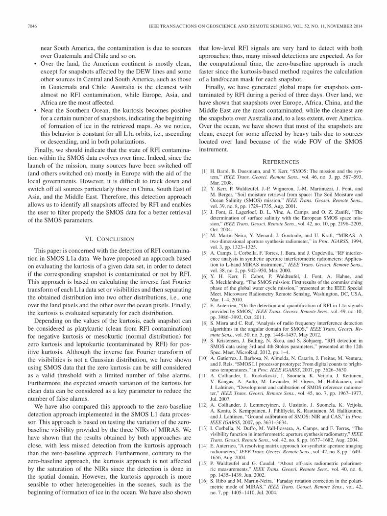
7046 IEEE TRANSACTIONS ON GEOSCIENCE AND REMOTE SENSING, VOL. 52, NO. 11, NOVEMBER 2014

near South America, the contamination is due to sourcesover Guatemala and Chile and so on.

• Over the land, the American continent is mostly clean,except for snapshots affected by the DEW lines and someother sources in Central and South America, such as thosein Guatemala and Chile. Australia is the cleanest withalmost no RFI contamination, while Europe, Asia, andAfrica are the most affected.

• Near the Southern Ocean, the kurtosis becomes positivefor a certain number of snapshots, indicating the beginningof formation of ice in the retrieved maps. As we notice,this behavior is constant for all L1a orbits, i.e., ascendingor descending, and in both polarizations.

Finally, we should indicate that the state of RFI contamina-tion within the SMOS data evolves over time. Indeed, since thelaunch of the mission, many sources have been switched off(and others switched on) mostly in Europe with the aid of thelocal governments. However, it is difficult to track down andswitch off all sources particularly those in China, South East ofAsia, and the Middle East. Therefore, this detection approachallows us to identify all snapshots affected by RFI and enablesthe user to filter properly the SMOS data for a better retrievalof the SMOS parameters.

VI. CONCLUSION

This paper is concerned with the detection of RFI contamina-tion in SMOS L1a data. We have proposed an approach basedon evaluating the kurtosis of a given data set, in order to detectif the corresponding snapshot is contaminated or not by RFI.This approach is based on calculating the inverse fast Fouriertransform of each L1a data set or visibilities and then separatingthe obtained distribution into two other distributions, i.e., oneover the land pixels and the other over the ocean pixels. Finally,the kurtosis is evaluated separately for each distribution.

Depending on the values of the kurtosis, each snapshot canbe considered as platykurtic (clean from RFI contamination)for negative kurtosis or mesokurtic (normal distribution) forzero kurtosis and leptokurtic (contaminated by RFI) for pos-itive kurtosis. Although the inverse fast Fourier transform ofthe visibilities is not a Gaussian distribution, we have shownusing SMOS data that the zero kurtosis can be still consideredas a valid threshold with a limited number of false alarms.Furthermore, the expected smooth variation of the kurtosis forclean data can be considered as a key parameter to reduce thenumber of false alarms.

We have also compared this approach to the zero-baselinedetection approach implemented in the SMOS L1 data proces-sor. This approach is based on testing the variation of the zero-baseline visibility provided by the three NIRs of MIRAS. Wehave shown that the results obtained by both approaches areclose, with less missed detection from the kurtosis approachthan the zero-baseline approach. Furthermore, contrary to thezero-baseline approach, the kurtosis approach is not affectedby the saturation of the NIRs since the detection is done inthe spatial domain. However, the kurtosis approach is moresensible to other heterogeneities in the scenes, such as thebeginning of formation of ice in the ocean. We have also shown

that low-level RFI signals are very hard to detect with bothapproaches; thus, many missed detections are expected. As forthe computational time, the zero-baseline approach is muchfaster since the kurtosis-based method requires the calculationof a land/ocean mask for each snapshot.

Finally, we have generated global maps for snapshots con-taminated by RFI during a period of three days. Over land, wehave shown that snapshots over Europe, Africa, China, and theMiddle East are the most contaminated, while the cleanest arethe snapshots over Australia and, to a less extent, over America.Over the ocean, we have shown that most of the snapshots areclean, except for some affected by heavy tails due to sourceslocated over land because of the wide FOV of the SMOSinstrument.

REFERENCES

[1] H. Barré, B. Duesmann, and Y. Kerr, “SMOS: The mission and the sys-tem,” IEEE Trans. Geosci. Remote Sens., vol. 46, no. 3, pp. 587–593,Mar. 2008.

[2] Y. Kerr, P. Waldteufel, J.-P. Wigneron, J.-M. Martinuzzi, J. Font, andM. Berger, “Soil moisture retrieval from space: The Soil Moisture andOcean Salinity (SMOS) mission,” IEEE Trans. Geosci. Remote Sens.,vol. 39, no. 8, pp. 1729–1735, Aug. 2001.

[3] J. Font, G. Lagerloef, D. L. Vine, A. Camps, and O. Z. Zanifé, “Thedetermination of surface salinity with the European SMOS space mis-sion,” IEEE Trans. Geosci. Remote Sens., vol. 42, no. 10, pp. 2196–2205,Oct. 2004.

[4] M. Martin-Neira, Y. Menard, J. Goutoule, and U. Kraft, “MIRAS: Atwo-dimensional aperture synthesis radiometer,” in Proc. IGARSS, 1994,vol. 3, pp. 1323–1325.

[5] A. Camps, I. Corbella, F. Torres, J. Bara, and J. Capdevila, “RF interfer-ence analysis in synthetic aperture interferometric radiometers: Applica-tion to L-band MIRAS instrument,” IEEE Trans. Geosci. Remote Sens.,vol. 38, no. 2, pp. 942–950, Mar. 2000.

[6] Y. H. Kerr, F. Cabot, P. Waldteufel, J. Font, A. Hahne, andS. Mecklenburg, “The SMOS mission: First results of the commissioningphase of the global water cycle mission,” presented at the IEEE SpecialMeet. Microwave Radiometry Remote Sensing, Washington, DC, USA,Mar. 1–4, 2010.

[7] E. Anterrieu, “On the detection and quantification of RFI in L1a signalsprovided by SMOS,” IEEE Trans. Geosci. Remote Sens., vol. 49, no. 10,pp. 3986–3992, Oct. 2011.

[8] S. Misra and C. Ruf, “Analysis of radio frequency interference detectionalgorithms in the angular domain for SMOS,” IEEE Trans. Geosci. Re-mote Sens., vol. 50, no. 5, pp. 1448–1457, May 2012.

[9] S. Kristensen, J. Balling, N. Skou, and S. Sobjaerg, “RFI detection inSMOS data using 3rd and 4th Stokes parameters,” presented at the 12thSpec. Meet. MicroRad, 2012, pp. 1–4.

[10] A. Gutierrez, J. Barbosa, N. Almeida, N. Catarin, J. Freitas, M. Ventura,and J. Reis, “SMOS L1 processor prototype: From digital counts to bright-ness temperatures,” in Proc. IEEE IGARSS, 2007, pp. 3626–3630.

[11] A. Colliander, L. Ruokokoski, J. Suomela, K. Veijola, J. Kettunen,V. Kangas, A. Aalto, M. Levander, H. Greus, M. Hallikainen, andJ. Lahtinen, “Development and calibration of SMOS reference radiome-ter,” IEEE Trans. Geosci. Remote Sens., vol. 45, no. 7, pp. 1967–1977,Jul. 2007.

[12] A. Colliander, J. Lemmetyinen, J. Uusitalo, J. Suomela, K. Veijola,A. Kontu, S. Kemppainen, J. Pihlflyckt, K. Rautiainen, M. Hallikainen,and J. Lahtinen, “Ground calibration of SMOS: NIR and CAS,” in Proc.IEEE IGARSS, 2007, pp. 3631–3634.

[13] I. Corbella, N. Duffo, M. Vall-llossera, A. Camps, and F. Torres, “Thevisibility function in interferometric aperture synthesis radiometry,” IEEETrans. Geosci. Remote Sens., vol. 42, no. 8, pp. 1677–1682, Aug. 2004.

[14] E. Anterrieu, “A resolving matrix approach for synthetic aperture imagingradiometers,” IEEE Trans. Geosci. Remote Sens., vol. 42, no. 8, pp. 1649–1656, Aug. 2004.

[15] P. Waldteufel and G. Caudal, “About off-axis radiometric polarimet-ric measurements,” IEEE Trans. Geosci. Remote Sens., vol. 40, no. 6,pp. 1435–1439, Jun. 2002.

[16] S. Ribo and M. Martin-Neira, “Faraday rotation correction in the polari-metric mode of MIRAS,” IEEE Trans. Geosci. Remote Sens., vol. 42,no. 7, pp. 1405–1410, Jul. 2004.

KHAZÂAL et al.: KURTOSIS APPROACH TO DETECT RFI IN SMOS IMAGE RECONSTRUCTION DATA PROCESSOR 7047

[17] P. Waldteufel, E. Anterrieu, J. Goutoule, and Y. Kerr, “Field of viewcharacteristics of a microwave 2D interferometric antenna as illustratedby the MIRAS concept,” in Proc. Microrad, 1999, pp. 477–483.

[18] L. DeCarlo, “On the meaning and use of kurtosis,” Radio Sci., vol. 2,no. 3, pp. 292–307, Sep. 1997.

[19] I. Kaplansky, “A common error concerning kurtosis,” J. Amer. Statist.Assoc., vol. 40, no. 230, pp. 259–263, 1945.

[20] J. Bezy, G. Gourmelon, R. B. G. Baudin, H. Sontag, and S. Weiss, “TheENVISAT Medium Resolution Imaging Spectrometer (MERIS),” in Proc.IEEE IGARSS, 1999, vol. 2, pp. 1432–1434.

[21] B. Tabachnick and L. Fidell, Using Multivariate Statistics, 3rd ed.New York, NY, USA: Harper Collins, 1996.

Ali Khazâal was born in Ansarieh, Lebanon,in 1981. He received the Engineer degree intelecommunication and computer science from TheLebanese University, Beirut, Lebanon, in 2003, theM.S. degree in signal, image, acoustic, and opti-mization from the Institut National Polytechnique,Toulouse, France, in 2006, and the Ph.D. degree insignal/image processing and optimization in 2009from the Paul Sabatier University, Toulouse, wherethe subject of his thesis was the image reconstructionalgorithms for the Soil Moisture and Ocean Salinity

(SMOS) mission, working with the Signal, Image and Instrumentation Group;Laboratoire d’Astrophysique de Toulouse-Tarbes; Observatoire Midi-Pyrénées.

Since October 2009, he has been a Research Scientist with the Center forthe Study of the BIOsphere (CESBIO), Universitè de Toulouse, CNRS, CNES& IRD, Toulouse. His current research interests include numerical analysisand signal and image processing, with direct application on European SpaceAgency’s SMOS mission.

François Cabot received the Ph.D. degree in opticalsciences from the University of Paris-Sud, Orsay,France, in 1995.

Between 1995 and 2004, he was with the CNESWide-Field-of-View Instrument Quality AssessmentDepartment, working on absolute and relative cali-bration of CNES-operated optical sensors over nat-ural terrestrial targets. In 2004, he joined the Centerfor the Study of the BIOsphere (CESBIO), Univer-sitè de Toulouse, CNRS, CNES & IRD, Toulouse,France, as an SMOS System Performance Engineer.

His research interests include radiative transfer both optical and microwave andremote sensing of terrestrial surfaces. He has been a Principal Investigator orCo-Investigator for various calibration studies for MSG, Terra, ENVISAT, andADEOS-II.

Eric Anterrieu (M’02) was born in Brive, France, in1965. He received the Engineer and M.S. degrees insolid-state physics from the Institut National des Sci-ences Appliquées, Toulouse, France, in 1988 and theM.S. and Ph.D. degrees in image reconstruction inastronomy, in 1989 and 1992, respectively, from thePaul Sabatier University, Toulouse, France, wherethe subject of his thesis was the image reconstructionalgorithms for multiple-aperture interferometry.

He is currently with the Signal, Image, and Instru-mentation Group; Research Institute of Astrophysics

and Planetology; Observatoire Midi-Pyrénées; Toulouse. Since 1993, he hasbeen an Engineer of research in computer science with the Centre Nationalde la Recherche Scientifique. His current research interests include numericalanalysis and image and signal processing, with particular emphasis on theSMOS project.

Yan Soldo received the Ph.D. degree in remote sensing in 2013 from the PaulSabatier University, Toulouse, France, where the subject of his thesis was theoptimization of the image reconstruction algorithms for SMOS and SMOSnext.

He is currently with the Center for the Study of the BIOsphere (CESBIO),Universitè de Toulouse, CNRS, CNES & IRD, Toulouse, France. His researchinterests include microwave and remote sensing, and he has also been interestedin the localization and mitigation of radio-frequency interferences in SMOSimages.