Receptive field formation in natural scene environments: comparison of

single cell learning rules

Brian S. Blais N. Intrator∗ H. Shouval Leon N Cooper

Brown University Physics Department and

Institute for Brain and Neural Systems

Brown University

Providence, RI 02912

{bblais,nin,hzs,lnc}@cns.brown.edu

February 23, 1998

Abstract

We study several statistically and biologically motivated learning rules using the same visual environment,

one made up of natural scenes, and the same single cell neuronal architecture. This allows us to concentrate on

the feature extraction and neuronal coding properties of these rules. Included in these rules are kurtosis and

skewness maximization, the quadratic form of the BCM learning rule, and single cell ICA. Using a structure

removal method, we demonstrate that receptive fields developed using these rules depend on a small portion

of the distribution. We find that the quadratic form of the BCM rule behaves in a manner similar to a

kurtosis maximization rule when the distribution contains kurtotic directions, although the BCM modification

equations are computationally simpler.

∗On leave, School of Mathematical Sciences, Tel-Aviv University.

1

1 Introduction

Recently several learning rules that develop simple cell-like receptive fields in a natural image environment have

been proposed (Law and Cooper, 1994; Olshausen and Field, 1996; Bell and Sejnowski, 1997). The details of

these rules are different as well as some of their computational reasoning, however they all depend on statistics

of order higher than two and they all produce sparse distributions.

In a sparse distribution most of the mass of the distribution is concentrated around zero, and the rest of the

distribution extends much farther out. In other words, a neuron that has sparse response, responds strongly to a

small subset of patterns in the input environment and weakly to all others. Bi-modal distributions, for which the

mode at zero has significantly more mass then the non-zero mode, and exponential distributions are examples of

sparse distributions, whereas Gaussian and uniform distributions are not considered sparse. It is known that many

projections of the distribution of natural images have long-tailed, or exponential, distributions (Daugman, 1988;

Field, 1994). It has further been argued that local linear transformations such as Gabor filters or center-surround

produce exponential-tailed histogram (Ruderman, 1994). Reasons given vary from the specific arrangements of

the Fourier phases of natural images (Field, 1994) to the existence of edges. Since the exponential distribution

is optimal from the view point of information theory under the assumption of positive and fixed average activity

(Ruderman, 1994; Levy and Baxter, 1996; Intrator, 1996; Baddeley, 1996), it is a natural candidate for detailed

study in conjunction with neuronal learning rules.

In what follows we investigate several specific modification functions that have the general properties of

BCM synaptic modification functions (Bienenstock et al., 1982) , and study their feature extraction properties

in a natural scene environment. BCM synaptic modification functions are characterized by a negative region

for small post-synaptic depolarization, a positive region for large post-synaptic depolarization, and a threshold

which moves and switches between the Hebbian and anti-Hebbian regions. Several of the rules we consider are

derived from standard statistical measures (Kendall and Stuart, 1977), such as skewness and kurtosis, based on

polynomial moments. We compare these with the quadratic form of BCM (Intrator and Cooper, 1992), though

one should note that this is not the only form that could be used. By subjecting all of the learning rules to the

same input statistics and retina/LGN preprocessing and by studying in detail the single neuron case, we eliminate

2

possible network/lateral interaction effects and can examine the properties of the learning rules themselves.

We start with a motivation for the learning rules used in this study, and then present the initial results.

We then explore some of the similarities and differences between the rules and the receptive fields they form .

Finally, we introduce a procedure for directly measuring the sparsity of the representation a neuron learns; this

gives us another way to compare the learning rules, and a more quantitative measure of the concept of sparse

representations.

2 Motivation

We use two methods for motivating the use of the particular rules. One comes from Projection Pursuit (Fried-

man, 1987), where we use an energy function to find directions where the projections of the data are non-

Gaussian(Huber, 1985, for review); the other is Independent Component Analysis (Comon, 1994), where one

seeks directions where the projections are statistically independent. These methods are related, as we shall see,

but they provide two different approaches for the current work.

2.1 Exploratory projection pursuit and feature extraction

Diaconis and Freedman (1984) show that for most high-dimensional clouds (of points), most low-dimensional

projections are approximately Gaussian. This finding suggests that important information in the data is conveyed

in those directions whose single dimensional projected distribution is far from Gaussian. There is, however,

some indication (Zetzsche, 1997) that for natural images, random local projections yield somewhat longer tailed

distributions than Gaussian. We can still justify this approach, because interesting structure can still be found

in non-random directions which yield projections that are farther from Gaussian.

Intrator (1990) has shown that a BCM neuron can find structure in the input distribution that exhibits

deviation from Gaussian distribution in the form of multi-modality in the projected distributions. This type

of deviation, which is measured by the first three moments of the distribution, is particularly useful for finding

clusters in high dimensional data through the search for multi-modality in the projected distribution rather than

3

in the original high dimensional space. It is thus useful for classification or recognition tasks. In the natural

scene environment, however, the structure does not seem to be contained in clusters: projection indices which

seek clusters never find them. In this work we show that the BCM neuron can still find interesting structure in

non-clustered data.

The most common measures for deviation from Gaussian distribution are skewness and kurtosis which are

functions of the first three and four moments of the distribution respectively. Rules based on these statistical

measures satisfy the BCM conditions proposed in Bienenstock et al. (1982), including a threshold-based stabi-

lization. The details of these rules and some of the qualitative features of the stabilization are different, however.

Some of these differences are seemingly important, while others seem not to affect the results significantly. In

addition, there are some learning rules, such as the ICA rule of Bell and Sejnowski (1997) and the sparse coding

algorithm of Olshausen and Field (1995), which have been used with natural scene inputs to produce oriented

receptive fields. We do not include these in our comparison because the learning is not based on the activity and

weights of a single neuron, and thus detract from our immediate goal of comparing rules with the same input

structure and neuronal architecture.

2.2 Independent Component Analysis

Recently it has been claimed that the independent components of natural scenes are the edges found in simple cells

(Bell and Sejnowski, 1997). This was achieved through the maximization of the mutual entropy of a set of mixed

signals. Others (Hyvarinen and Oja, 1997) have claimed that maximizing kurtosis, with the proper constraints,

can also lead to the separation of mixed signals into independent components. This alternate connection between

kurtosis and receptive fields leads us into a discussion of ICA.

Independent Component Analysis (ICA) is a statistical signal processing technique whose goal is to express

a set of random variables as linear combinations of statistically independent variables. We observe k scalar

variables (d1, d2, . . . , dk)T ≡ d which are assumed to be linear combinations of n unknown statistically independent

4

variables (s1, s2, . . . , sn)T. We can express this mixing of the sources s as

d = As (2.1)

where A is an unknown k×n mixing matrix. The problem of ICA is then to estimate both the mixing matrix A

and the sources s using only the observation of the mixtures di. Using the feature extraction properties of ICA,

the columns of A represent features, and si represent the amplitude of each feature in the observed mixtures d.

These are the features in which we are interested.

In order to perform ICA, we first make a linear transformation of the observed mixtures

c = Md (2.2)

These linearly transformed variables would be the outputs of the neurons, in a neural network implementation

and M, the unmixing matrix or matrix of features, would be the weights. Two recent methods for performing

ICA (Bell and Sejnowski, 1995; Amari et al., 1996) involve maximizing the entropy of a non-linear function of the

transformed mixtures, σ(c), and minimizing the mutual information of σ(c) with respect to the transformation

matrix, M, so that the components of σ(c) are independent. These methods are, by their definition, multi-neuron

algorithms and therefore do not fit well into the framework of this study.

The search for independent components relies on the fact that a linear mixture of two non-Gaussian

distributions will become more Gaussian than either of them. Thus, by seeking projections c = (d ·m) which

maximize deviations from Gaussian distribution, we recover the original (independent) signals. This explains the

connection of ICA to the framework of exploratory projection pursuit (Friedman and Tukey, 1974; Friedman,

1987). In particular it holds for the kurtosis projection index, since a linear mixture will be less kurtotic than its

original components.

Kurtosis and skewness, have also been used for ICA as approximations of the negative entropy (Jones

and Sibson, 1987). It remains to be seen if the basic assumption used in ICA, that the signals are made up of

independent sources, is valid. The fact that different ICA algorithms, such as kurtosis and skewness maximization,

5

yield different receptive fields could be an indication that the assumption is not completely valid.

3 Synaptic modification rules

In this section we outline the derivation for the learning rules in this study, using either the method from

projection pursuit or independent component analysis. Neural activity is assumed to be a positive quantity, so

for biological plausibility we denote by c the rectified activity σ(d ·m) and assume that the sigmoid is a smooth

monotone function with a positive output (a slight negative output is also allowed). σ′ denotes the derivative

of the sigmoidal. The rectification is required for all rules that depend on odd moments because these vanish

in a symmetric distribution such as natural scenes. We also demonstrate later that the rectification makes little

difference on learning rules that depend on even moments.

We study the following measures:

Skewness 1 This measures the deviation from symmetry (Kendall and Stuart, 1977, for review) and is of the

form:

S1 = E[c3]/E1.5[c2]. (3.3)

A maximization of this measure via gradient ascent gives

∇S1 =1

ΘM1.5E

[c(c−E[c3]/E[c2]

)σ′d]

=1

ΘM1.5E

[c(c−E[c3]/ΘM

)σ′d]

(3.4)

where Θm is defined as E[c2].

Skewness 2 Another skewness measure is given by

S2 = E[c3]−E1.5[c2]. (3.5)

6

This measure requires a stabilization mechanism, because it is not invariant under constant multiples of the

activity c. We stabilize the rule by requiring that the vector of weights, which is denoted by m, has a fixed norm,

say ‖m ‖= 1. The gradient of this measure is

∇S2 = 3E[c2 − c

√E[c2]

]= 3E

[c(c−

√ΘM

)σ′d], (3.6)

subject to the constraint ‖m ‖= 1.

Kurtosis 1 Kurtosis measures deviation from Gaussian distribution mainly in the tails of the distribution. It

has the form

K1 = E[c4]/E2[c2]− 3. (3.7)

This measure has a gradient of the form

∇K1 =1

ΘM2E[c(c2 −E[c4]/E[c2]

)σ′d]

=1

ΘM2E[c(c2 −E[c4]/ΘM

)σ′d]. (3.8)

Kurtosis 2 As before, there is a similar form which requires some stabilization:

K2 = E[c4]− 3E2[c2]. (3.9)

This measure has a gradient of the form

∇K2 = 4E[(c3 − 3cE[c2]

)σ′d]

= 4E[c(c2 − 3ΘM)σ′d

], ‖m ‖= 1. (3.10)

In all the above, the maximization of the measure can be used as a goal for projection seeking. The variable c

can be thought of as a (nonlinear) projection of the input distribution onto a certain vector of weights, and the

maximization then defines a learning rule for this vector of weights. The multiplicative forms of both kurtosis

7

and skewness do not require an extra stabilization constraint.

Kurtosis 2 and ICA It has been shown (Hyvarinen and Oja, 1996) that kurtosis, defined as

K2 = E[c4]− 3E2

[c2]

can be used for ICA. This can be seen by using the property of this kurtosis measure, K2(x1 + x2) = K2(x1) +

K2(x2) for independent variables, and defining z = ATm. We then get

K2(m · d) ≡ K2(mTd) = K2(mTAs) = K2(zTs) =n∑j=1

z4jK2(sj) (3.11)

The extremal points of Equation 3.11 with respect to z under the constraint E[(m · d)2

]= 1 occur when one

component zj of z is ±1 and all the rest are zero (Delfosse and Loubaton, 1995). In other words, finding the

extremal points of kurtosis leads to projections where m ·d ≡mTd = zTs equals, up to a sign, a single component

sj of s. Thus, finding the extrema of kurtosis of the projections enables the estimation of the independent

components individually, rather than all at once, as is done by other ICA rules. A full ICA code could be

developed by introducing a lateral inhibition network, for example, but we restrict ourselves to the single neuron

case here for simplicity.

Maximizing K2 under the constraint E[(m · d)2

]= 1, and defining the covariance matrix of the inputs

C = E[ddT

], yields the following learning rule

m =2λ

(C−1E

[d(m · d)3

]− 3m

). (3.12)

This equation leads to an iterative “fixed-point algorithm”, which converges very quickly and works both for

single cell and network implementations.

8

Quadratic BCM The Quadratic BCM (QBCM) measure as given in (Intrator and Cooper, 1992) is of the

form

QBCM =13E[c3]− 1

4E2[c2]. (3.13)

Maximizing this form using gradient ascent gives the learning rule:

∇QBCM = E[c2 − cE[c2]

]= E[c(c−ΘM)σ′d]. (3.14)

Unlike the measures S2 and K2 above, the Quadratic BCM rule does not require any additional stabilization. This

turns out to be an important property, since additional information can then be transmitted using the resulting

norm of the weight vector m (Intrator, 1996).

4 Methods

We use 13x13 circular patches from 12 images of natural scenes as the visual environment. Two different types

of preprocessing of the images are used for each of the learning rules. The first is a Difference of Gaussians

(DOG) filter, which is commonly used to model the processing done in the retina (Law and Cooper, 1994). The

second is a whitening filter, used to eliminate the second order correlations (Oja, 1995; Bell and Sejnowski, 1995).

Whitening the data in this way allows one to use learning rules which are dependent on higher moments of the

data, but are particularly sensitive to the second moment.

At each iteration of the learning, a patch is taken from the preprocessed (either DOGed or whitened)

images and presented to the neuron. The moments of the output, c, are calculated iteratively using

E[cn(t)] =1τ

∫ t

−∞cn(t′)e−(t−t′)/τdt′

In the cases where the learning rule is under-constrained (i.e. K2 and S2) we also normalize the weights at each

iteration.

9

For Oja’s fixed-point algorithm, the learning was done in batches of 1000 patterns over which the ex-

pectation values were performed. However, the covariance matrix was calculated over the entire set of input

patterns.

5 Results

5.1 Receptive Fields

The resulting receptive fields (RFs) formed are shown in Figures 1 and 2 for both the DOGed and whitened

images, respectively. Each RF shown was achieved using different random initial conditions for the weights.

Every learning rule developed oriented receptive fields, though some were more sensitive to the preprocessing

than others. The additive versions of kurtosis and skewness, K2 and S2 respectively, developed significantly

different RFs in the whitened environment compared with the DOGged environment. The RFs in the whitened

environment had higher spatial frequency and sampled from more orientations than the RFs in the DOGed

environment. This behavior, as well as the resemblance of the receptive fields in the DOGed environment to

those obtained from PCA (Shouval and Liu, 1996), suggest that these measures have a strong dependence on the

second moment.

The multiplicative versions of kurtosis and skewness, K1 and S1 respectively, as well as Quadratic BCM,

sampled from many orientations regardless of the preprocessing. The multiplicative skewness rule, S1, gives

receptive fields with lower spatial frequencies than either Quadratic BCM or the multiplicative kurtosis rule.

This also disappears with the whitened inputs, which implies that the spatial frequency of the receptive field is

related to the strength of the dependence of the learning rule on the second moment. Example receptive fields

using Oja’s fixed-point ICA algorithm are also shown in Figure 2, and not surprisingly look qualitatively similar

to those found using the stochastic maximization of additive kurtosis, K2.

The log of the output distributions for all of the rules have the double linear form, which implies a double

exponential distribution. This distribution is one which we would consider sparse, but it would be difficult to

compare the sparseness of the distributions merely on the appearance of the output distribution alone. In order

10

to determine the sparseness of the code, we introduce a method for measuring it directly.

Receptive Fields from Natural Scene Input: DOGed

DO

Ged

−10 0 100

5

10Output Distribution

BCM

−10 0 100

5

10K

1

−10 0 100

5

10K

2

−10 0 100

5

10S

1

−10 0 100

5

10S

2

Figure 1: Receptive fields using DOGed image input obtained from learning rules maximizing (from top to bottom)the Quadratic BCM objective function, Kurtosis (multiplicative), Kurtosis (additive), Skewness (multiplicative),and Skewness (additive). Shown are five examples (left to right) from each learning rule as well as the log of thenormalized output distribution, before the application of the rectifying sigmoid.

5.2 Structure Removal: Sensitivity to Outliers

Learning rules which are dependent on large polynomial moments, such as Quadratic BCM and kurtosis, tend

to be sensitive to the tails of the distribution. This property implies that neurons are highly responsive, and

sensitive, to the outliers, and consequently leads to a sparse coding of the input signal. One should note that

over-sensitivity to outliers is considered to be undesirable in the statistical literature. However, in the case of

a sparse code the outliers, or the rare and interesting events, are what is important. The degree to which the

neurons form a sparse code determines how much of the input distribution is required for maintaining the RF.

This can be done in a straightforward and systematic fashion.

The procedure involves simply eliminating from the environment those patterns for which the neuron

responds strongly. An example receptive field and some of the patterns which give that neuron strong responses

11

Receptive Fields from Natural Scene Input (Whitened)

Whi

tene

d

BCM

−0.1 0 0.10

5

10Output Distribution

K1

−0.1 0 0.10

5

10

K2

−0.1 0 0.10

5

10

S1

−0.1 0 0.10

5

10

S2

−0.1 0 0.10

5

10

Oja ICA using K2

−0.1 0 0.10

5

10

Figure 2: Receptive fields using whitened image input, obtained from learning rules maximizing (from top to bot-tom) the Quadratic BCM objective function, Kurtosis (multiplicative), Kurtosis (additive), Skew (multiplicative),Skewness (additive), and Oja’s ICA rule based on the additive kurtosis measure. Shown are five examples (leftto right) from each learning rule as well as the log of the normalized output distribution, before the applicationof the rectifying sigmoid.

is shown in Figure 3. These patterns tend to be the high contrast edges, and are thus the structure found in

the image. The percentage of patterns that needs to be removed in order to cause a change in the receptive

field gives a direct measure of the sparsity of the coding. The process of training a neuron, eliminating patterns

which yield high response, and retraining can be done recursively to sequentially remove structure from the input

environment, and to pick out the most salient features in the environment. The results of this are shown in

Figure 4.

For Quadratic BCM and kurtosis, one need only eliminate less than one half of a percent of the input

patterns to change the receptive field significantly. The changes which one can observe include orientation, phase

and spatial frequency changes. This is a very small percentage of the environment, which suggests that the neuron

12

Structure in the Image

Figure 3: Patterns which yield high responses of a model neuron. The example receptive field is shown on theleft. Some of the patterns which yield the strongest 1/2 percent of responses are labeled on the image on theright. These patterns are primarily the high contrast edges.

is coding the information in a very sparse manner. For the skewness maximization rule, more than five percent

are needed to alter the receptive field properties, which implies a far less sparse coding.

To make this more precise, we introduce a normalized difference measure between two different RFs. If we

take two weight vectors, m1 and m2, then the normalized difference between them is defined as

D ≡ 14

(m1 − m̄1

‖m1 ‖− m2 − m̄2

‖m2 ‖

)2

(5.15)

=12

(1− cosα) (5.16)

where α is the angle between the two vectors, and m̄i is the mean of the elements of the vector i. This measure

is not sensitive to scale differences, because the vectors are divided by their norm, and it is not sensitive to scalar

offset differences, because the mean of the vectors is subtracted. The measure has a value of zero for identical

vectors, and a maximum value of one for orthogonal vectors.

Shown in Figure 5 is the normalized difference as a function of the percentage eliminated, for the different

learning rules. Differences can be seen with as little as a tenth of a percent, but only changes of around half a

percent or above are visible as significant orientation, phase, or spatial frequency changes. Although both skewness

and Quadratic BCM depend primarily on the third moment, Quadratic BCM behaves more like kurtosis with

regards to projections from natural images.

Similar changes occur for both the BCM and kurtosis learning rules, and most likely occur under other

rules that seek kurtotic projections. It is important to note, however, that patterns must be eliminated from

13

both sides of the distribution for any rule that does not use the rectifying sigmoid because the strong negative

responses carry as much structure as the strong positive ones. Such responses are not biologically plausible, so

they wouldn’t be part of the encoding process in real neurons.

It is also interesting to observe that the RF found after structure removal is initially of the same orientation,

but of different spatial phase or possibly different position. Once enough input patterns are removed, the RF

becomes oriented in a different direction. If the process is continued, all of the orientations and spatial locations

would be obtained.

An objection may be made that the receptive fields formed are caused almost entirely by the application

of the rectifying sigmoid. For odd powered learning rules, the sigmoid is necessary to obtain oriented receptive

fields because the distributions are approximately symmetric. This sigmoid is not needed for rules dependent

only on the even powered moments, such as kurtosis. Figure 6 demonstrates that the removal of the sigmoid and

the removal of the mean from the moments calculations do not substantially affect the resulting receptive fields

of the kurtosis rules.

The choice of 13 by 13 pixel receptive fields was biologically motivated and computationally less demanding

than larger receptive fields formation. Figure 7 shows some 21 by 21 pixel receptive fields and it is clear that

little difference is observed. One may notice that the length of the receptive field is larger than the lengths of the

RFs found using Olshausen and Field’s or Bell and Sejnowski’s algorithms. It is likely that events causing such

elongated RF’s are very rare, and thus lead to higher kurtosis. When additional constraints are imposed such as

finding a complete code, one ends up with less specialized receptive fields and thus, less elongated RFs.

14

Structure Removal for BCM, Kurtosis, and Skew

BCM

K1

S1

Figure 4: Receptive fields resulting from structure removal using the Quadratic BCM rule, the rule maximizing

the multiplicative form of kurtosis and skewness. The RF on the far left for each rule was obtained in the normal

input environment. The next RF to the right was obtained in a reduced input environment, whose patterns were

deleted that yielded the strongest 1% of responses from the RF to the left. This process was continued for each

RF from left to right, yielding a final removal of about five percent of the input patterns.

Structure Removal for BCM, Kurtosis, and Skew

10−2

10−1

100

101

0

0.05

0.1

0.15

0.2

0.25

0.3

Nor

mal

ized

diff

eren

ce in

RF

Percent removed

BCM Kurtosis 1Skew 1

Figure 5: Normalized difference between RFs as a function of the percentage deleted in structure removal. The

RFs were normalized, and mean zero, in order to neglect magnitude and additive constant changes. The maximum

possible value of the difference is 1.

15

6 Discussion

This study attempts to compare several learning rules which have some statistical or biological motivation, or

both. For a related study discussing projection pursuit and BCM see (Press and Lee, 1996). We have used natural

scenes to gain some more insight about the statistics underlying natural images. There are several outcomes from

this study:

• All rules used, found kurtotic distributions. This should not come as a surprise as there are suggestions

that a large family of linear filters can find kurtotic distributions (Ruderman, 1994).

• The single cell ICA rule we considered, used the subtractive form of kurtosis as a measure for deviation

from Gaussian distributions, achieved receptive fields qualitatively similar to other rules discussed.

• The Quadratic BCM and the multiplicative version of kurtosis are less sensitive to the second moments of

the distribution and produce oriented receptive fields even when the data is not whitened. This is clear

from the results about DOG-processed vs. whitened inputs. The reduced sensitivity follows from the built

in second order normalization that these rules have, kurtosis via division and BCM via subtraction. The

subtractive version of kurtosis is sensitive and produces oriented RF only after sphering the data (Friedman,

1987; Field, 1994).

• Both Quadratic BCM and kurtosis are sensitive to the tails of the distribution. In fact, the RF changes due

to elimination of the upper 1/2% portion of the distribution (Figure 4). The change in RF is gradual; at

first, removal of some of the inputs results in RFs that have the same orientation but a different phase, once

more patterns from the upper portion of the distribution are removed, different RF orientations are found.

This finding gives some indication to the kind of inputs the cell is most selective to (values below its highest

99% selectivity), these are inputs with same orientation but with different phase (different locality of RF).

The sensitivity to small portions of the distribution represents the other side of the coin of sparse coding.

It should be further studied as it may reflect some fundamental instability of the kurtotic approaches.

• The skewness rules can also find oriented RF’s. Their sensitivity to the upper parts of the distribution is

not so dramatic and thus, the RFs do not change much when few percent of the upper distribution are

16

removed.

• Kurtotic rules can find high kurtosis in either symmetric or rectified distributions. This is not the case for

Quadratic BCM rule which requires rectified distributions.

• Quadratic BCM learning rule, which has been advocated as a projection index for finding multi-modality in

high dimensional distribution, can find projections emphasizing high kurtosis when no cluster structure is

present in the data. We have preliminary indications that the converse is not true, namely, kurtosis measure

does not perform well under distributions that are bi- or multi-modal. This will be shown elsewhere.

17

Exploring Modifications to the Kurtosis rules

−10 0 100

5

10Output Distribution

K1 with sigmoid

−10 0 100

5

10

K1 without sigmoid

−10 0 100

5

10

K1 without sigmoid and centered moments

−10 0 100

5

10

K2 with sigmoid

−10 0 100

5

10

K2 without sigmoid

−10 0 100

5

10

K2 without sigmoid and centered moments

Figure 6: Receptive fields using DOGed image input, obtained from learning rules maximizing (from top to

bottom) multiplicative form kurtosis with rectified outputs, non-rectified outputs, and non-rectified outputs with

centered moments respectively, and additive form kurtosis with rectified outputs, non-rectified outputs, and non-

rectified outputs with centered moments respectively. Shown are five examples (left to right) from each learning

rule and the corresponding output distribution.

18

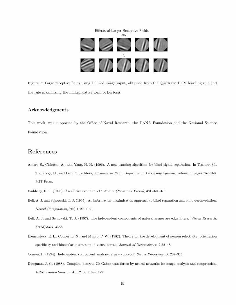
Effects of Larger Receptive Fields

BCM

K1

Figure 7: Large receptive fields using DOGed image input, obtained from the Quadratic BCM learning rule and

the rule maximizing the multiplicative form of kurtosis.

Acknowledgments

This work, was supported by the Office of Naval Research, the DANA Foundation and the National Science

Foundation.

References

Amari, S., Cichocki, A., and Yang, H. H. (1996). A new learning algorithm for blind signal separation. In Tesauro, G.,

Touretzky, D., and Leen, T., editors, Advances in Neural Information Processing Systems, volume 8, pages 757–763.

MIT Press.

Baddeley, R. J. (1996). An efficient code in v1? Nature (News and Views), 381:560–561.

Bell, A. J. and Sejnowski, T. J. (1995). An information-maximisation approach to blind separation and blind deconvolution.

Neural Computation, 7(6):1129–1159.

Bell, A. J. and Sejnowski, T. J. (1997). The independent components of natural scenes are edge filters. Vision Research,

37(23):3327–3338.

Bienenstock, E. L., Cooper, L. N., and Munro, P. W. (1982). Theory for the development of neuron selectivity: orientation

specificity and binocular interaction in visual cortex. Journal of Neuroscience, 2:32–48.

Comon, P. (1994). Independent component analysis, a new concept? Signal Processing, 36:287–314.

Daugman, J. G. (1988). Complete discrete 2D Gabor transforms by neural networks for image analysis and compression.

IEEE Transactions on ASSP, 36:1169–1179.

19

Delfosse, N. and Loubaton, P. (1995). Adaptive blind separation of independent sources: a deflation approach. Signal

Processing, 45:59–83.

Field, D. J. (1994). What is the goal of sensory coding. Neural Computation, 6:559–601.

Friedman, J. H. (1987). Exploratory projection pursuit. Journal of the American Statistical Association, 82:249–266.

Friedman, J. H. and Tukey, J. W. (1974). A projection pursuit algorithm for exploratory data analysis. IEEE Transactions

on Computers, C(23):881–889.

Huber, P. J. (1985). Projection pursuit. (with discussion). The Annals of Statistics, 13:435–475.

Hyvarinen, A. and Oja, E. (1996). A fast fixed-point algorithm for independent component analysis. Int. Journal of Neural

Systems, 7(6):671–687.

Hyvarinen, A. and Oja, E. (1997). A fast fixed-point algorithm for independent component analysis. Neural Computation,

9(7).

Intrator, N. (1990). A neural network for feature extraction. In Touretzky, D. S. and Lippmann, R. P., editors, Advances

in Neural Information Processing Systems, volume 2, pages 719–726. Morgan Kaufmann, San Mateo, CA.

Intrator, N. (1996). Neuronal goals: Efficient coding and coincidence detection. In Amari, S., Xu, L., Chan, L. W., King, I.,

and Leung, K. S., editors, Proceedings of ICONIP Hong Kong. Progress in Neural Information Processing, volume 1,

pages 29–34. Springer.

Intrator, N. and Cooper, L. N. (1992). Objective function formulation of the BCM theory of visual cortical plasticity:

Statistical connections, stability conditions. Neural Networks, 5:3–17.

Jones, M. C. and Sibson, R. (1987). What is projection pursuit? (with discussion). J. Roy. Statist. Soc., Ser. A(150):1–36.

Kendall, M. and Stuart, A. (1977). The Advanced Theory of Statistics, volume 1. MacMillan Publishing, New York.

Law, C. and Cooper, L. (1994). Formation of receptive fields according to the BCM theory in realistic visual environments.

Proceedings National Academy of Sciences, 91:7797–7801.

Levy, W. B. and Baxter, R. A. (1996). Energy efficient neural codes. Neural Computation, 8:531–543.

Oja, E. (1995). The nonlinear pca learning rule and signal separation - mathematical analysis. Technical Report A26,

Helsinki University, CS and Inf. Sci. Lab.

Olshausen, B. A. and Field, D. J. (1996). Emergence of simple cell receptive field properties by learning a sparse code for

natural images. Nature, 381:607–609.

20

Press, W. and Lee, C. W. (1996). Searching for optimal visual codes: Projection pursuit analysis of the statistical

structure in natural scenes. In The Neurobiology of Computation: Proceedings of the fifth annual Computation and

Neural Systems conference. Plenum Publishing Corporation.

Ruderman, D. L. (1994). The statistics of natural images. Network, 5(4):517–548.

Shouval, H. and Liu, Y. (1996). Principal component neurons in a realistic visual environment. Network, 7(3):501–515.

Zetzsche, C. (1997). Intrinsic dimensionality: how biological mechanisms exploit the statistical structure of natural images.

Talk given at the Natural Scene Statistics Meeting.

21