Micro-economics I BCM -121
117
Micro-economics I BCM - 121 Prepared by: Yordanos Gebremeskel
Transcript of Micro-economics I BCM -121

Micro-economics I BCM - 121
Prepared by: Yordanos Gebremeskel

Contents ------------------------------------------------------------ Page
UNIT ONE -------------------------------------------------------------------------------------------------------------------------- 2
FOUNDATION OF ECONOMICS------------------------------------------------------------------------------------------------ 2
INTRODUCTION ------------------------------------------------------------------------------------------------------------------- 2 1.1 Economics and Economic System --------------------------------------------------------------------------------- 3
1.1.1 What you study in Economics? ----------------------------------------------------------------------------------------- 3 1.1.2 Distinction between Macroeconomics and Microeconomics ---------------------------------------------------- 4 1.1.3 Microeconomics and Choice -------------------------------------------------------------------------------------------- 5 1.1.4 Economic Systems -------------------------------------------------------------------------------------------------------- 6 1.1.5 Kinds of economic system ----------------------------------------------------------------------------------------------- 6
1.2 Using Diagrams and models in Economics --------------------------------------------------------------------- 8 1.3 Scarcity, Choice and Opportunity cost --------------------------------------------------------------------------- 8 1.4 Rational choices ---------------------------------------------------------------------------------------------------- 10 1.5 The Production Possibility Curve -------------------------------------------------------------------------------- 11
Unit Summary ---------------------------------------------------------------------------------------------------------- 14 Unit Assignment-------------------------------------------------------------------------------------------------------- 15
UNIT TWO ------------------------------------------------------------------------------------------------------------------------ 16
MARKET, SUPPLY AND DEMAND ------------------------------------------------------------------------------------------- 16
INTRODUCTION ----------------------------------------------------------------------------------------------------------------- 16 2.1 Markets and Prices ------------------------------------------------------------------------------------------------ 17
2.1.1 Basic features of a market --------------------------------------------------------------------------------------------- 17 2.1.2 Addressing economic problems in a market system ------------------------------------------------------------- 18
2.2 Demand -------------------------------------------------------------------------------------------------------------- 19 2.2.1 Individual and Market Demand -------------------------------------------------------------------------------------- 19 2.2.2 The Law of Demand----------------------------------------------------------------------------------------------------- 19 2.2.3 The Demand Schedule ------------------------------------------------------------------------------------------------- 20 2.2.4 The Demand Curve------------------------------------------------------------------------------------------------------ 21 2.2.5 Exceptions to the Law of Demand ----------------------------------------------------------------------------------- 22 2.2.6 Determinants of Market Demand------------------------------------------------------------------------------------ 23 2.2.7 Movements along and shifts in the demand curve --------------------------------------------------------------- 25
2.3 Supply ----------------------------------------------------------------------------------------------------------------- 26 2.3.1 Market Supply ----------------------------------------------------------------------------------------------------------- 26 2.3.2 The Law of Supply ------------------------------------------------------------------------------------------------------- 27 2.3.3 The Supply Schedule ---------------------------------------------------------------------------------------------------- 28 2.3.4 The supply curve -------------------------------------------------------------------------------------------------------- 28 2.3.5 Other Determinants of Supply ---------------------------------------------------------------------------------------- 29 2.3.6 Movements along and shifts in the supply curve ----------------------------------------------------------------- 31
2.3 Equilibrium of Demand and Supply ---------------------------------------------------------------------------- 31 2.3.1 The Concept of Equilibrium ------------------------------------------------------------------------------------------- 32 2.3.2 Determination of market price --------------------------------------------------------------------------------------- 32 2.3.3 Shift in Demand or Supply Curve and Market Equilibrium ------------------------------------------------------ 33
2.3.3.1 Shift in Demand Curve and Market Equilibrium ------------------------------------------------------------ 34 2.3.3.2 Shift in the Supply Curve and Market Equilibrium --------------------------------------------------------- 34
2.3.4 Algebra of Demand, Supply and Equilibrium ---------------------------------------------------------------------- 35 2.3.4.1 Demand Function ------------------------------------------------------------------------------------------------- 35 2.3.4. 2 Supply function --------------------------------------------------------------------------------------------------- 36 2.3.4.3 Demand – Supply Equilibrium ---------------------------------------------------------------------------------- 37
Unit Summary ---------------------------------------------------------------------------------------------------------- 39 Unit Assignment-------------------------------------------------------------------------------------------------------- 40

Unit One
Foundation of economics
Introduction
Unit one of this module is an introductory unit to the study of
economics. Microeconomics being one branch of economics, it is useful
to start first by introducing what economics is all about. In this unit,
emphasis is also given to basic concepts and methodologies that are
significantly useful in the whole learning of economics.
Upon completion of this unit, you will be able to answer basic questions
like:
What is economics?
What is an economic system?
What is microeconomics and macroeconomics?
What is scarcity, choice and opportunity cost?

1.1 Economics and Economic System
1.1.1What you study in Economics?
Economics is concerned with addressing different economic questions that relate with
individuals, households, society and the economy in general. For instance, why students
like you decide to pursue additional education by paying fees? How does a given firm
(factory) decide what to produce, how much to produce and how to produce? How the
prices of copper and other minerals are determined in national and international markets?
How is the value of 1 Kwacha expressed with other currencies like Euro or USD? What
is the reason behind the 2008/2009 economic recession in most developed countries and
its impact on other developing countries? Economics addresses these and other questions
systematically and logically by analyzing economic units’ behavior.
Definitions of Economics
There is no universally accepted single definition of economics. Different
economists defined economics in different ways. Let us look at some of
the definitions made by prominent economists.
Economics is “an inquiry into the nature and causes of the wealth
of nations”
Adam Smith
“Economics is the science which studies human behavior as a
relationship between ends and scarce means which have
alternative uses”
Lionel Robbins
“Economics is the study of humankind in the ordinary business of
life; it examines that part of individual and social action which is
most closely connected with the attainment and with the use of the
material requisites of well being”
Alfred Marshall

“Economics is the study of how men and society choose, with or
without the use of money, to employ the scarce productive
resources which could have alternative uses, to produce various
commodities over time and distribute them for consumption now
and in the future amongst various people and groups of society”
Paul A. Samuelson
In general, economics is the study of the process and technique of
making choices and making allocation of resources aimed at maximizing
the gains. Economics also studies:
The total outcome of the economic activities of the people
participating in the economy.
The determination of national income, saving, investment and
growth of national income.
Trends in general price level, supply and demand of money and
their impact on the economy, public revenue and public
expenditure, economic policies and financial transactions, and
economic transactions among countries.
1.1.2 Distinction between Macroeconomics and Microeconomics
Economics is traditionally divided into two main branches called
Microeconomics and Macroeconomics. The prefixes, „micro‟ and „macro‟
have been derived from Greek words where „mikros = micro‟ means small
and „makros = macro‟ means big.
When an economic study deals with economic behavior of an individual
decision making unit (consumer and producer) or and economic variable
(price and quantity of a good) it is Microeconomics. And, when an
economic study deals with economic aggregates like national income,
general employment, aggregate consumption, savings and investment,

general price level and balance of payments position, etc is called
Macroeconomics.
There are a number of branches of economics under the umbrella of
microeconomics or macroeconomics. Some of these are Welfare
Economics, Resource Economics, Health Economics, Labor Economics
and International Economics.
1.1.3 Microeconomics and Choice
Because resources are scarce, choices have to be made by individuals,
groups or the government in order to address what is called the three
basic economic questions. Choices must be made in any society
regarding:
What and how much to produce. That is, what goods and services
are going to be produced and in what quantities, since there are
not enough resources to produce all the things people desire?
How to produce. That is, how are things going to be produced,
given that there is normally more than one way of producing
things? What resources are going to be used and in what
quantities? What techniques of production are going to be
adopted?
For whom to produce. That is, for whom are things going to be
produced? In other words, how will the nation‟s income be
distributed?
These three economic problems can be solved differently by the type of
economic system a given nation has.

1.1.4 Economic Systems
An economic system is a social organization through which people make
their living. It is constituted of all those individuals, households, farms,
firms, factories, banks and government which act and interact to
produce and consume goods and services.
1.1.5 Kinds of economic system
Depending on the degree of government control of the economy,
economies are generally classified as:
i. planned or command economy
ii. free-market economy
iii. mixed economy
(i) Planned or command economy
In this type of economic system all the economic decisions are taken by
the government. These economies are largely controlled, regulated and
managed by government agencies. It is usually associated with a socialist
or communist economic system, where land and capital are collectively
owned. The three basic economic questions are addressed by the state.
The state plans the allocation of resources between current
consumption and investment for the future.
At a micro level, it plans the output of each industry and firm, the
techniques that will be used, and the labor and other resources
required by each industry and firm.
It plans the distribution of output between consumers.
(ii)The free-market economy

In a free market, individuals are free to make their own economic
decisions. In this type of economy there is less government intervention
at all.
Consumers are free to decide what to buy with their incomes: free
to make demand decisions.
Firms are free to choose what to sell and what production methods
to use: free to make supply decision.
The demand and supply decisions of consumers and firms are
transmitted to each other through their effect on prices: through
price mechanism.
The prices that result are the prices that firms and consumers
have to accept.
(iii) The mixed economy
In practice, all economies are a mixture of both planned and free-
market system. Therefore, we can say it is the degree of government
intervention that distinguishes different economic systems in the
world.
In mixed market economies, the government may be involved in
affecting:
Relative prices of goods and inputs, by taxing or subsidizing
them or by direct price controls.
Relative incomes, by the use of income taxes, welfare payments
or direct controls over wages, profits etc.
The pattern of production and consumption, by the use of
legislation (e.g. making illegal the production of drugs (cocaine,
heroin), by direct provision of goods and services (e.g. education
and defense), by taxes and subsidies or by nationalization.

The macroeconomic problems of unemployment, inflation,
tradebalance (Import-Export), foreign exchange rate, by the use
of taxes and government expenditure, the control of bank
lendingand interest rates, the direct control of prices and the
control of the foreign exchange rate.
1.2 Using Diagrams and models in Economics
Economics discussion frequently uses diagrams. The reasons are:
- Diagrams are very useful for illustrating economic relationships.
- They show simplified pictures of reality.
- Ideas and arguments that might take long time to explain in words
can often be expressed clearly and simply in a diagram.
Economics also use models to make quantitative predictions. A model is
a mathematical representation, based on economic theory, of a firm, a
market or some other entity.
1.3 Scarcity, Choice and Opportunity cost
‘You can’t always get what you want’
Individuals, society and government have to make choices because of
certain basic facts of human life. These facts are related to human
beings‟ endless wants and the reality of there are only limited resources
in the world at any given time.
Human wants and desires are unlimited. The poor people as well as the
wealthiest people desire to consume more and better of different goods
and services. In general human wants are virtually unlimited.
The endless human wants are attributable to:

People have insatiable desire to raise their standard of living to a
level as high as possible.
Human nature is accumulative, i.e., people accumulate things
beyond their present need.
Human wants multiply with growth of human knowledge, science
and technology, which lead to production of new goods through
inventions and innovations.
Human wants are multiplicative. Introduction of a new commodity
create need for many others. For example, purchase of a car
creates demand for petrol, driver, parking place, spare parts,
insurance, etc.
Since resources (income) are not sufficient to satisfy all the wants
simultaneously, consumers have to make choice among their wants –
which wants to fulfill now and which want to fulfill later.
Resources are limited and scarce. While human wants are unlimited,
resources that are available to satisfy human wants are limited. At any
one time the world can only produce a limited amount of goods and
services. – The world only has limited amount of resources. These
resources (factors of production) are broadly classified as:
Human resource: the labor available both in number and skill at
any point of time is limited. Labor is limited by the size of
population.
Natural resource: land and raw materials are limited by the area of
a country.
Manufactured resource: The man-made resources like capital and
technology are limited by the scarcity of inputs that go into their
production, such as, Limited supplies of factories, machines,
transportation, telecommunication and other equipment. The
productivity of capital is also limited by the state of technology.
Furthermore, choice involves sacrifice. The more food you choose to buy,
the less money you will have to spend on other goods like fees for
education or buying a house. The more food a nation produces the fewer
resources will there be for producing other goods.
→The production and consumption of one thing involves the
sacrifice/ trade-off of other alternatives.
This sacrifice/ trade-off of alternatives in consumption or production of a
good or service is known as its opportunity cost.
→ The opportunity cost of any activity is the sacrifice made to do it.
It is the best thing that could have been done as an alternative.
→ It is the cost of the explicit and implicit resources that are
forgone when a decision is made.
Example: Assume the farmer can produce either 10,000 kgs of
wheat or 15,000 kgs of maize on his land. Thus, the opportunity
cost of producing 1 kg of wheat is 1.5 kgs of maize forgone. The
opportunity cost of overtime work could be the leisure (social affair)
you have sacrificed.
1.4 Rational choices
The assumption of rational choice is central for studying behavior of
economic units (individuals, firms, society and government). It simply

means, economic units weigh-up costs and benefits when they make
whatever economic decisions. For instance:
- Firms calculate costs and benefits when choosing what and how
much to produce
- Workers consider costs and benefits when choosing whether to
take a particular job or to work extra hours.
- Consumers do the same when they decide what to buy.
Particularly for consumers, a rational decision making refers choosing
those items that give you the best value for money, that is, the greatest
benefit relative to cost.
1.5The Production Possibility Curve
Production possibility curve is a curve that shows all the possible
combinations of two goods that a firm or for that matter a country can
produce within a specified time period with all its resources fully and
efficiently employed.
Example: Assume Zambia allocates all its resources (land, labor
and capital) for producing two goods, i.e., food and clothing.
Table 1.1 Maximum possible combinations of maize and copper that can
be produced in a given time period

From the above table you can see that, Zambia by allocating all its
resources for producing maize could produce 8 metric tons of maize but
no copper. Alternatively, by producing 6 metric tons of maize it could
release enough resources to produce 4 metric tons of copper in addition.
The information in the table can be translated into the following graph.
Units of maize
(in metric tons)
Units of copper
(in metric tons)
8 0
7 2
6 4
5 5
4 5.6
3 6
2 6.4
1 6.7
0 7

Figure 1.1 Production possibility curve for copper and maize
The above production possibilities curve (PPC) shows the maximum
combinations of output that the economy can produce using all
available resources. The curve displays a trade-off, that is, more of
maize production implies less of copper production (example point A).
The PPC shows the points at which the economy is producing
efficiently using the available resources and technologies. Points
above the PPC are unattainable points (example point D, because it
requires more resource than the economy has available).
Whereas, points inside the PPC (example point E) are attainable but
inefficient – since it indicates there are idle resources which can
increase production of both goods if used efficiently.
E
A
B
C
D
0
1
2
3
4
5
6
7
8
0 1 2 3 4 5 6 7 8 9
Co
pp
er
in m
etr
ic t
on
es
Maize (in metric tones)
production possibility curve

Unit Summary Economics is the study of the process and technique of making
choices and making allocation of resources aimed at maximizing
the gains among individuals, households, firms, societies,
countries and so forth.
Economics is divided into two main branches. These are
microeconomics and macroeconomics.
The study of microeconomics deals with economic behavior of an
individual decision making unit (consumer and producer) or and
economic variable (price and quantity of a good).
The study of macroeconomics deals with economic aggregates like
national income, general employment, aggregate consumption,
savings and investment, general price level and balance of
payments position, etc is called Macroeconomics.
Any economic system must address the three basic economic
questions of what to produce, how to produce and for whom to
produce.
Since resources are scarce every human being is forced to make
choices for every economic activity. Every choice entails
opportunity cost.
The assumption of rational choice is central for studying behavior
of economic units or economic agents.
Production possibility curve shows all the possible combinations of
two goods that a country can produce within a specified time
period with all its resources fully and efficiently employed.
Unit Review Questions 1. The study of economics generally lies in the endless wants and
scarcity of resources. Explain
2. Do you think the study of microeconomics and macroeconomics
are exclusively separated studies? Why?
3. What is the relationship between scarcity, rational choice and
opportunity cost?
4. How do you interpret the economic difference between developed
countries and resource abundant poor countries using the PPF
model?

Unit Two
Market, Supply and Demand
Introduction
In this unit you will learn about the functioning of a market economic
system and its basic problems. How the three economic problems are
addressed in the market economic system and the role of price in this
system will be discussed. Mathematical application of theory of demand
and supply is also attached as an annex. This will give you a chance to
refresh your high school mathematics knowledge and to alert you, there
will be some mathematical applications of microeconomics in subsequent
chapters.
Upon completion of this unit you will be able to:
Understand and discuss the meaning and features of a market
Understand and discuss the role of price in a market economic
system
Understand and define the concepts of demand, supply and
market equilibrium
Familiarize and discuss different factors that affect demand,
supply and market equilibrium
2.1 Markets and Prices
In economics a market means a system in which sellers and buyers of a
commodity interact to settle the price and the quantity to be bought and
sold. The sellers and buyers may be individuals, firms, factories, dealers
and agents.
2.1.1 Basic features of a market
A market need not be situated in a particular place or locality. The
size of the market stretches from a local fish or vegetable market to
a worldwide market for automobiles, copper or medicines.
Buyers and sellers need not always come in personal contact with
each other. The transaction can be conducted through agents,
telephone, fax, postal services and internet.
The word „market‟ refers to either a commodity or service (e.g., fish
market, automobile market, money market, entertainment market)
or a geographical area (e.g., Lusaka market, London market,
Europe market).
In economics markets are further distinguished on the basis of
(1) On the nature of goods and services, e.g., factor market and
commodity market / input market and output market.
(2) Number of firms and degree of competition, e.g., competitive
market, monopoly market, Oligopolistic market and monopolistic
competitive market.
In unit one you recall that, the way the three basic economic problems
are addressed depends on the nature of the economic system. There we
said, in a free market system, the problems are solved by the market

(price) mechanism. Now let us see how the price mechanism solves the
basic economic problems in a free market economy system.
2.1.2 Addressing economic problems in a market system
What to produce?
The goods and services that are produced in a market economy are
determined by consumer demand. Only those goods and services which
are demanded by the consumers or users are produced by the producers.
Therefore, every kwacha a consumer spends on a commodity is treated
as a vote for producing that commodity. Continuing demand is a
continuous process of voting.
How to produce?
It is the question of choice of technology, that is, the proportion of labor,
capital and raw material used to produce a commodity. The choice of
resource combination is also determined by the market forces of supply
and demand.
For whom to produce?
The market rule for this problem is – produce for those who have ability
and willingness to pay. That is, in a free market mechanism, goods and
services are produced for those who possess the ability to pay.
Market (price) mechanism is a process through which the market
economy functions. The market economy functions through the market
forces of demand and supply. The demand and supply forces interact to

determine the price of goods and services. Therefore, a price system is
generated. The system is operated by, what Adam Smith called „invisible
hands’, i.e., the market forces of demand and supply.
Prices perform two functions in the market system.
1. Prices serve as signals for the producers to decide „what to
produce‟ and for the consumers to decide „what to consume‟.
2. Prices force the demand and supply conditions to adjust
themselves to the prevailing prices.
2.2 Demand
Demand can be defined as the desire for a good for whose fulfillment a
person has sufficient resources and willingness to pay for the good. A
desire without sufficient money income is a simple desire, not demand. A
desire with resources but without willingness to pay is a potential
demand.
→ A desire accompanied by ability and willingness to pay makes
the Real or Effective Demand.
2.2.1 Individual and Market Demand
Individual Demand can be defined as the quantity of a commodity that a
person is willing to buy at a given price over a specified period of time –
per day, per week or per month. On the other hand, Market Demand is
the total quantity that all consumers of a commodity are willing to buy at
given price over a specific period of time.
→ Market demand is the sum of individual demands.
2.2.2 The Law of Demand

The Law of Demand states the relationship between the quantity
demanded and price of a commodity. The law of demand is generally
associated with price. This is because, price is the most and often the
only determinant in the short-run period. In fact, we have other factors
which also affect the quantity demand and we will discuss them shortly.
→ Law of demand:All other things remaining constant, the quantity
demanded of a commodity increases when its price decreases and it
decreases when its price increases.
The law implies that quantity and price changes are inversely related.
The law of demand can be easily discussed by using a demand schedule
and demand curve.
2.2.3 The Demand Schedule
Demand Schedule is a tabular presentation of a series of prices of a
commodity with the corresponding quantities demanded. Let us consider
the following example.
Table 2.1 Demand schedule for maize
Price per kg (in
kwacha)
2,000 1,800 1,600 1,400 1,200 1,000
Quantity demanded (in
kgs)
100 150 200 300 400 500
Table 2.1 clearly illustrates the law of demand. As the price of maize
decreases, we can see that the demand for maize increases. For instance,
when price of maize is 2,000k, 100 kgs of maize is demanded per day.

When price decreases by half, i.e., to 1,000k, the demand for maize
increases to 500 kgs per day.
2.2.4 The Demand Curve
A Demand Curve is a graphical representation of the law of demand. The
demand curve can be obtained by plotting the demand schedule on a two
dimension graph.
Figure 2.1 Demand curve for maize
The curve DD is the Demand curve. The curve reflects the law of demand
and it is a downward curve to the right. It has a negative slope. The
negative slope of a demand curve shows the inverse relationship between
D
B
A
D
0
1,000
2,000
3,000
4,000
5,000
6,000
7,000
8,000
9,000
0 20 40 60 80 100
Pri
ce o
f m
aiz
e (
in k
wach
a)
Quantity of maize (in kgs)

quantity demanded of maize and price of maize. It shows that demand
for maize increases as the price decreases and vice versa.
Why Demand Curve Slopes Downward to the Right?
The reasons behind the downward sloping demand curve or law of
demand are:
A. Income Effect: when the price of a commodity falls, the real income of
its consumers increases in terms of this commodity. In other words,
consumers‟ purchasing power increases since they are required to pay
less for the same quantity. Furthermore, increase in real income (or
purchasing power) increases demand for goods and services in general
and for the good with reduced price in particular. The increase in
demand due to an increase in income is called income effect.
B. Substitution Effect: when price of a commodity falls, it becomes
cheaper compared to its substitutes, other prices remaining constant, or,
the substitute becomes more costly. In general, consumers tend to
substitute cheaper goods for costly ones. The increase in demand on
account of this factor is called substitution effect.
2.2.5 Exceptions to the Law of Demand
The law of demand does not apply to the following cases:
I. Expectations regarding future prices: when consumers expect a
continuous increase in the price of a durable commodity, they buy
more of it despite increase in its price to avoid the burden of still
higher price in future. Similarly, sometimes consumers anticipate

a considerable decrease in the price in the future and they
postpone their purchases by waiting for the price to fall further.
II. Prestigious goods: the law of demand also does not apply to the
commodities which serve as a „status symbol‟ or display wealth
and richness. Example, gold, diamond, paintings and antiques.
These goods are still demanded by rich people despite their prices
increasing.
III. Giffen goods:the other exception to this law is the case of Giffen
goods named after Robert Giffen (1837 – 1910). A Giffen goods
does not mean any specific commodity. It may be any essential
commodity much cheaper than its substitutes, consumed mostly
by the poor households claiming a large part of their incomes. If
price of such goods increases (price of its substitute remaining
constant), its demand increases instead of decreasing.
2.2.6 Determinants of Market Demand
Until now we have discussed demand by holding everything constant
other than the price. But there are other factors than the price of a good
which influence demand. The following are the major demand affecting
factors in addition to price.
(i)Income
The consumer‟s income is the basic determinant of the quantity
demanded of a product. Because income affects the ability of consumers
to purchase a good, changes in income affect how much consumers will
buy at any price. That is why the people with higher disposable income
spend a larger amount of money on goods and services than those with
lower income.

In graphical terms, a change in income shifts the entire demand curve.
Whether an increase in income shifts the demand curve to the right or to
the left depends on the nature of consumer consumption pattern.
Accordingly, economists distinguish between two types of goods: normal
and inferior goods.
Normal goods
A good whose demand increases (a right shift in the demand curve)
when consumers‟ incomes rise is called a normal good. Food,
clothes, household furniture are some of the examples of this
category. As income goes up, consumers typically buy more of
these goods at any given price. Conversely, when consumers suffer
a decline in income, the demand for a normal good will decrease
(shift to the left).
Inferior goods
Sometimes, an increase in income reduces the demand for a good.
As income goes up, consumers typically consume less of these
goods at each price. But, you need to be careful for not interpreting
inferior goods as goods of poor quality. We use this term simply to
define products that consumers purchase less of it when their
incomes rise, and purchase more of it when their incomes fall.
(ii)The number and price of substitute goods (competitive goods)
Two commodities are considered to be substitutes for each other if a
change in the price of one affects the demand for the other in the same
direction. For example, tea and coffee, Pepsi and Coca cola, hamburger
and hot dog are common substitutes. The relation between demand for a
product and the price of its substitute is positive. When price of product
(say, tea) falls, then demand for its substitute (coffee) falls.
(iii) The number and price of complementary goods
Complementary goods are those that are consumed together. For
example, car and petrol, shoe and polish are common complimentary.
Technically, two goods are complement for one another if an increase in
the price of one causes a decrease in the demand for another. There is
aninverse relationship between the demand for a good and the price of its
complement. An increase in the price of petrol causes a decrease in the
demand for car, other things remaining the same.
(iv) Consumer‟s taste and preference
Consumer‟s taste and preferences play an important role in determining
the demand for a product. The more desirable people find the good, the
more they will demand. Taste and preferences depend, generally on the
social customs, values attached to a commodity, habits of the people, age
and sex of the consumers. For example, Zambians are highly attached to
their staple food Nshima. In today‟s modern world, tastes are also
affected by advertising, by fashion, by observing other consumers and by
considerations of health.
2.2.7 Movements along and shifts in the demand curve
The effect of a change in price on quantity demanded is simply a
movement along the demand curve. For example, in figure 2.1, a move
from point A to point B is caused by a change in price. In general we call
this change (move) a change in quantity demanded. In other words, any
change that arises from change in price is change in quantity demanded

and it is explained by movement along the same demand curve. Whereas
a change in other demand affecting factors than price leads to a change
in demand. If a change in one of the other determinants causes demand
to rise – say, income rises – the whole curve will shift to the right.
Generally, a change in demand is explained by a shift in the entire
demand curve.
A rightward shift in the demand curve is called an increase in demand,
since more of the good is demanded at each price. A leftward shift in the
demand curve is called a decreasein demand.
Figure 2.2 Movements along and shifts in demand curve
2.3 Supply
In a market economy, while buyers of a product constitute the demand
side of the market, sellers of that product make the supply side of the
market.
2.3.1 Market Supply

Supply means the quantity of a commodity which its producers or sellers
offer to sell at a given price, per unit of time. Market supply, like market
demand, is the sum of supplies of a commodity made by individual firms.
2.3.2 The Law of Supply
The supply of a commodity depends on its price and cost of production.
That is, supply is the function of price and production cost. The law of
supply is, however, expressed generally in terms of price-quantity
relationship. The law of supply can be stated as:
→ The supply of a product increases with the increase in its price
and decreases with decrease in its price, other things remaining
constant.
There are three reasons for this:
The higher the price of the good, the more profitable it becomes to
produce. That is, firms will be encouraged to produce more.
Given time, if the price of good remains high, new producers will
be encouraged to participate in production. Thus, total market
supply will increase.
As producers supply more, they are likely to find that beyond a
certain level of output, costs rise more and more rapidly. For
instance, costs are likely to rise as production increases because it
requires employing more workers, more payment for over time and
utilizing the machines to their maximum working capacity. If
higher output involves higher costs of producing each unit,
producers will need to get a higher price if they are to produce
additional output.

2.3.3 The Supply Schedule
The supply schedule is a tabular presentation of the law of supply. It
shows alternative price of a commodity and the corresponding quantity
that suppliers are willing to supply. Let us consider the following
example.
Table 2.2 Supply schedule for canned beef
Price
(in kwacha)
10,000 20,000 30,000 40,000 55,000 75,000
Supply (canned
beef in pcs)
10,000 35,000 50,000 60,000 75,000 80,000
From the table you can see that at price level of 10,000k per canned beef,
only 10 thousand canned beef are supplied per month. When prices
increase to 20,000, suppliers offer 35,000 canned beef and, when price
increased as much as 75,000 per canned beef, supply rises to 80
thousand canned beef.
2.3.4 The supply curve
The supply schedule can be represented graphically as a supply curve. In
figure 2.3 the curve SS is the Supply curve. The curve reflects the law of
supply and it is an upward curve to the right. In contrast to a demand
curve, a supply curve has a positive slope.

Figure 2.3 Supply curve for canned beefs
2.3.5 Other Determinants of Supply
Although price of a commodity is the most important determinant of
supply, there are also other factors that influence the supply of a
commodity.
(i) The costs of production
The higher the costs of production, the less profit will be made at any
price. As costs rise, firms will reduce production. The main reasons for a
change in costs are as follows:
S
A
B
C
S
0
10,000
20,000
30,000
40,000
50,000
60,000
70,000
80,000
90,000
0 20,000 40,000 60,000 80,000 100,000
Pri
ce (
in k
wach
a)
Quantity supplied (canned beef)

Change in input prices: costs of production will increase if payment
for labor, raw materials and capital increase.
Change in technology: Technological changes that reduce cost of
production or increase efficiency increase the product supply.
Organizational changes: A lot of cost can be saved by reorganizing
the production system.
Government policy: Firm‟s cost may increase (example due to
higher tax) or decrease (example by getting subsidy).
Labor productivity: Firms could enjoy efficiency in cost
minimization as they recruit the required proportionate amount of
skilled labor with other inputs (such as capital).
(ii)Price of alternative products (substitutes in supply)
In many kinds of production activities, it is possible to produce a
substitute product. If a product which is a substitute in supply becomes
more profitable to supply than before, producers are likely to switch from
the first good to this alternative. For example if a refrigerator price goes
up the company may decide to reduce the production of Air conditioners‟
production in order to produce more refrigerators.
(iii)Expectation of future price changes
If price is expected to rise, producers may temporarily reduce the amount
they sell. In order to gain more from future higher price, they tend to
keep the stocks.

(iv) Number of Suppliers.
If size of the industry increases due to new firms joining the industry, the
total supply will increase.
2.3.6 Movements along and shifts in the supply curve
The effect of a change in price on quantity supplied is simply a movement
along the supply curve. For example, in figure 2.3, a move from point A to
point B or from B to C is caused by a change in price. In general we call
this change (move) a change in quantity supplied. In other words, any
change that arises from change in price is change in quantity supplied
and it is explained by movement along the same supply curve. Whereas,
a change in other supply affecting factors than price leads to a change in
supply. Generally, a change in supply is explained by a shift in the entire
supply curve.
A rightward shift in the supply curve illustrates an increase in supply,
since more of the good is supplied at each price. A leftward shift in the
demand curve on the other hand illustrates a decreasein supply.
2.3 Equilibrium of Demand and Supply
In the previous sections, you have seen the demand and supply sides of
the market and how demand and supply behave in response to a change
in price and other factors. Now, we can combine the analysis of demand
and supply and see how they form a balance, how market attains
equilibrium, and how equilibrium price is determined in a free market
and competitive market.

2.3.1 The Concept of Equilibrium
The term equilibrium means the „state of rest‟ – a point where conflicting
interests are balanced. It indicates the condition where forces working in
opposite direction are in balance. In market context:
→ Equilibrium refers to a state of market in which the quantity
demanded of a commodity equals the quantity supplied of the
commodity. The equality of demand and supply produces an
equilibrium price and output.
In general, at equilibrium price, demand and supply are in equilibrium.
And, the equilibrium price is called market-clearing price because at this
point a market clears when supply matches demand, leaving no shortage
or surplus.
2.3.2 Determination of market price
The equilibrium price in a free market is determined by the market forces
of demand and supply. Let us consider the following example to
understand how the market forces bring the suppliers‟ plan in balance
with the buyers‟ plan.
Table 2.3 Demand and supply schedule for maize
Price
(per kg)
Demand
for maize
(in kgs)
Supply
of maize
(in kgs)
Market
position
Effect on
price
1,200 400 100 Shortage Rise
1,400 300 150 Shortage Rise
1,600 200 200 Equilibrium Stable
1,800 150 250 Surplus Fall
2,000 100 300 Surplus Fall

As the above table shows you, there is a single price, 1,600K, at which
the market is in equilibrium. At this point the quantity demanded and
the quantity supplied is equal at 200 kgs of maize. Other price levels
than this indicatedisequilibrium in the market price. That is, there is
either an excess of demand over supply or an excess of supply over
demand. At all prices below 1,600 K, demand exceeds supply showing
shortage of maize in the market. Again, at all prices above 1,600 K
supply exceeds demand showing surplus supply.
Figure 2.4 Market equilibrium
Price
D S
Pe
S D
Qe Quantity
Graphically, market equilibrium is attained at the intersection point of
the demand curve (DD) and the supply curve (SS) as shown above in
figure 2.4. At the point of intersection the market clears out at a price
level of Pe and quantity level of Qe.
2.3.3 Shift in Demand or Supply Curve and Market Equilibrium
The equilibrium price will remain unchanged as long as the demand and
supply curves remain unchanged. But, a shift in either demand or
supply curves (due to other factors than price), will cause for a new
equilibrium to be formed.
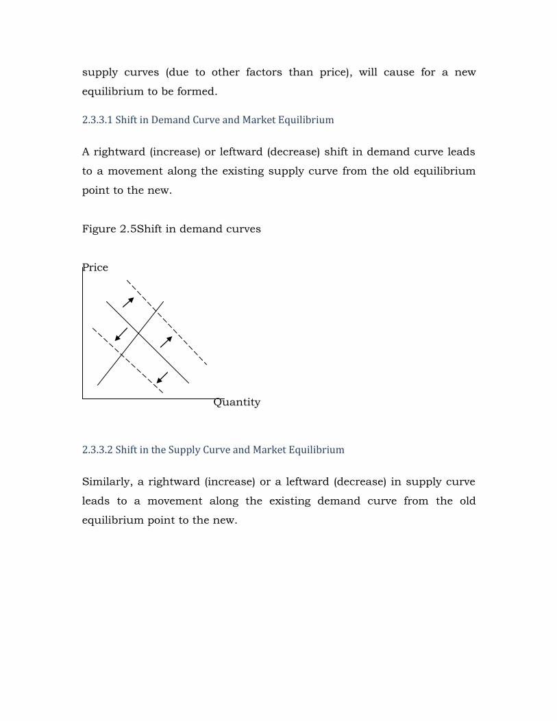
2.3.3.1 Shift in Demand Curve and Market Equilibrium
A rightward (increase) or leftward (decrease) shift in demand curve leads
to a movement along the existing supply curve from the old equilibrium
point to the new.
Figure 2.5Shift in demand curves
Price
Quantity
2.3.3.2 Shift in the Supply Curve and Market Equilibrium
Similarly, a rightward (increase) or a leftward (decrease) in supply curve
leads to a movement along the existing demand curve from the old
equilibrium point to the new.

Figure 2.6Shift in supply curves
Price
Quantity
2.3.4Algebra of Demand, Supply and Equilibrium
Beside graphical representation of demand, supply and equilibrium
analysis, economics often use algebraic representation for better clarity
and precision.
2.3.4.1Demand Function
Demand function represents the market demand for a good and the
determinants of demand in the form of equation.
The demand function for a commodity can take an equation form:
Qd = a – bP
Where, Qd is quantity demanded
P is price of the good
-b is slope of the demand curve (recall that quantity demand
and price are negatively related)
a is the constant term, which equals the quantity demanded
if price is zero.

This equation relates quantity demanded to price. In other words, the
equation assumed that all the other determinants of demand remain
constant (ceteris paribus). For example, the actual equation might be:
Qd = 100 – 5P
Now from this you can easily calculate a complete demand schedule and
demand curve by assigning a hypothetical price levels.
This simple equation can be expanded by incorporating other demand
affecting factors. For example demand function of the form:
Qd = a – bP + cY + dPs
describes that, the quantity demanded (Qd) is determined by price (P)
which is negatively related; level of consumer income(Y) which is
positively related; and price of the substitute good (Ps) which is positively
related.
2.3.4. 2Supply function
Likewise, supply function represents the market supply for a good and
the determinants of supply in the form of equation.
A supply function can take a form:
Qs = c + dP
Where, Qs is quantity supplied
P is the price f the good

d is slope of the supply curve (recall that quantity supplied
and price are positively related)
c is the constant term, which equals quantity supplied if
price is zero
This equation relates quantity supplied to price. In other words, the
equation assumed that all the other determinants of supply remain
constant (ceteris paribus). For example the actual equation might be:
Qs = 25P
Again by taking hypothetical values for price it is easy to construct both
supply schedule and supply curve.
More complex supply equations would relate supply to more than one
determinant. For instance:
Qs = 4 + 8P – 5Ps + 12Pc
This supply equation shows that, the quantity supplied (Qs) is
determined by price (P) which is positively related; price of substitute
goods(Ps) which is negatively related; and price of the complementary
good (Pc) which is positively related.
2.3.4.3Demand – Supply Equilibrium
Once we have the demand and supply functions it is easy to calculate
equilibrium price and equilibrium output levels.
Let us consider that supply and demand equation for a given market is
as follows:

Qd = a – bP (1)
Qs = c + dP (2)
Now we can find the market equilibrium price by setting the two
equations equal to each other – taking the fact that, equilibrium is a
situation where demand and supply are equal in the market.
c + dP = a – bP
Subtracting c form the left side and adding bP to both sides will give us:
dP + bP = a – c
(d + b)P = a – c
P = a – c
d + b (3)
For calculating equilibrium quantity (Q𝜖), we need to substitute equation
(3) in either the demand function - (1) or the supply function - (2).
Therefore, from equation (1)
Q𝜖 = a – b (a – c)
(d + b)
= a (d + b) – b(a – c)
d + b
= ad + ab – ba + bc
d + b
= ad + bc
d + b

or from equation (2)
Q𝜖= c + d (a – c)
(d + b)
= cd + cb + da − dc
d + b
= cb + da
d + b
Unit Summary Market is a system in which sellers and buyers of a commodity
interact to settle the price and the quantity to be bought and sold.
A market can be defined as a commodity or service, as a
geographical area, by the nature of goods and services or by the
number of firms and degree of competition.
While, Individual Demand refers to the quantity of a commodity
that a person is willing to buy at a given price over a specified
period of time; Market Demand is the total quantity that all
consumers of a commodity are willing to buy at given price over a
specific period of time.
The law of demand states that, the quantity demanded of a
commodity increases when its price decreases and it decreases
when its price increases holding other factors constant.
While Supply refers to the quantity of a commodity which its
producers or sellers offer to sell at a given price, per unit of time;
Market supply is the sum of supplies of a commodity made by
individual firms.
The law of supply states that, a product‟s supply increases with
the increase in its price and decreases with decrease in its price,
other factors remaining constant.

Equilibrium refers to a state of market in which the quantity
demanded of a commodity equals the quantity supplied of the
commodity.
Unit Review Questions 1. What is the difference among desire, effective demand and
potential demand?
2. What is the relationship between law of demand and the slope of a
demand curve?
3. Which demand factors cause a shift in the demand and supply
curves from their original positions?
4. Given the demand function Q= 30 – 5P, develop a demand
schedule and derive a demand curve?
5. From the demand function Qd = 100 – 15P and a supply function
Qs = 10P calculate,
(a) Equilibrium price
(b) Equilibrium quantity
(c) The gap between demand and supply at P=2 and P=6

Unit Three
Elasticity of Demand
Introduction
In this unit you will extend your knowledge of theory of demand to
understand a new concept known as elasticity of demand. As you recall,
the laws of demand and supply simply states the nature (not the extent)
of relationship between the changes in price and quantity demanded and
supplied respectively, at different price levels. But in most cases we want
to know by how much the quantity demanded or quantity supplied
changed for a given change in price.
Upon completion of this unit you will be able to
Define the concept of elasticity, price elasticity of demand and
income elasticity of demand.
Measure demand elasticity for changes in market price and
consumer‟s income.
Discuss the different uses of the concept of elasticity in economic
activities.

3.1 Price Elasticity of Demand
For certain types of goods, a given percentage change in price brings
about a small change in quantity demanded (quantity supplied),
whereas, for another good it will result in a big change. So, how much
are these small and big changes? This problem is addressed by the
measure of responsiveness of demand and supplyto change in price.
The price elasticity of demand is generally defined as the degree of
responsiveness or sensitiveness of demand for a commodity to the
changes in its price. That is, elasticity of demand is the percentage change
in the quantity demanded of a commodity as a result of a certain
percentage change in its price. We use percentage or proportionate
changes since price and quantity are measured in different units.
Price elasticity of demand is one of the most important concepts in
economics. For example, if we know the price elasticity of demand for a
product, we can easily predict the effect on price and quantity of a
change for an increase or decrease of supply.
3.1.1 Measuring the price elasticity of demand
In measuring price elasticity of demand our interest is in knowing the
size of change in quantity demanded with the size of the change in price.
The formula for the price elasticity of demand for a product is percentage
(or proportionate) change in quantity demanded divided by the
percentage (or proportionate) change in price.

A general formula for calculating coefficient of price-elasticity (PϵD) is:
PϵD = Percentage change in quantity demanded
Percentage change in price
=
𝑄1−𝑄0𝑄0
𝑃1−𝑃0𝑃0
= ∆Q
Qo÷
∆P
Po
We use the absolute value sign to avoid negative elasticity results
= ∆Q
Qo×
Po
∆P
Where Qo = original quantity demanded, Po = original price, ∆Q = change
in quantity demanded, and ∆P = change in price. We use the symbol 𝜖for
elasticity, and ∆ for a „change in‟.
Example: given original price (Po) = 10, new price (P1) = 20, original
quantity demanded (Qo) = 40, and new quantity (Q1) = 20
Thus, ∆P = (P1) − (Po) = 20 – 10 = 10 and
∆Q = (Q1) − (Qo) = 20 – 40 = −20
P𝜖D = ∆Q
Qo×
Po
∆P =
−20
40×
10
10 = −0.5 = 0.5
(Recall that the absolute value of any number is positive)

3.1.2 Interpreting elasticity figures
(i) The sign (positive or negative)
Demand curves are generally downward sloping. This means price and
quantity change in opposite direction. A rise in price (a positive figure)
will cause a fall in the quantity demanded (a negative figure). Likewise, a
fall in price will cause a rise in the quantity demanded. Therefore, our
final elasticity figure is negative and for convenience as we said above we
consider it as a positive value (but keeping in mind the inverse
relationship between price and quantity demanded).
(ii) The value (greater or less than 1)
As we have said, if we ignore the negative sign and concentrate on the
value of the figure, it tells us whether demand is elastic, inelastic or unit
elastic.
Elastic (𝜖> 1): This is where a change in price causes a
proportionately larger change in the quantity demanded. That is, a
case when 1 percentage change in price will brings about a more
than 1 percentage change in quantity demanded. The value of
elasticity will be greater than 1 since we are dividing a larger figure
by a smaller figure.
Inelastic (𝜖< 1): This is where a change in a price causes a
proportionately smaller change in the quantity demanded. That is,
a case when 1 percentage change in price will brings about a less
than 1 percentage change in quantity demanded. The value of
elasticity will be less than 1 since we are dividing a smaller figure
by a larger figure.

Unit elastic (𝜖 = 1): Unitary elasticity of demand occurs where price
and quantity demanded change by the same proportion. That is, a
case when 1 percentage change in price will brings about an equal
1 percentage change in quantity demanded. The value of elasticity
will be equal to 1 since we are dividing equal figures.
3.1.3 Determinants of price elasticity of demand
The elasticity of demand varies from commodity to commodity. While the
demand for some commodities is highly elastic, for some it is highly
inelastic. What determines price elasticity of demand?
i. Number and closeness of substitute goods: this is the most
important determinant. The more substitutes there are for a good,
and the closer they are, the greater will be the elasticity of demand
for a commodity. For instance, consider coffee and tea as close
substitutes for one another. If price of coffee increases, then tea
becomes relatively cheaper and consumers switch to the
consumption of more tea.
Beside closeness, the wider the range of the substitutes, the
greater will be the elasticity. For instance, soaps, toothpastes,
cigarettes are available in different brands, each brand being a
close substitute for the other.
ii. Nature of commodity: commodities can be in general grouped as
luxuries and necessities. Demand for luxury goods (cars, costly TV
sets, decoration items etc) is more elastic because consumption of
these goods can be postponed when their prices rise. On the other
hand demand for necessity goods (food, cloths, electricity, water
etc) cannot be postponed, and hence their demand is inelastic.

iii. The proportion of income spent on the good: if proportion of income
spent on a commodity is very small, its demand will be less elastic,
and vice versa. For instance salt and matches have a very low price
elasticity of demand. Part of the reason is that there are no close
substitutes. But part is that we spend a small fraction of our
income on these goods that we would find little difficulty in paying
a relatively large percentage increase in prices. On the other hand,
the higher the proportion of our income we spend on a good, the
more we will be forced to cut consumption when its price rises.
iv. Time factor: price elasticity of demand also depends on the time
consumers take to adjust to a new price – the longer the time
taken, the greater will be the elasticity. When price rises, people
may take time to adjust their consumption patterns and find
alternatives. For instance, if price of cars is decreased demand will
not immediately increase unless people possess strong purchasing
power.
3.1.4 Special cases in price elasticity of demand
i. Totally inelastic demand (P𝜖D = 0): No matter what happens to
price, quantity demanded remains the same.
ii. Infinitely elastic demand (P𝜖D = ∞): At any price above P1 demand is
zero. But at P1 (or any price below) demand is infinitely large.
iii. Unit elastic demand (P𝜖D = 1): this is where price and quantity
change in exactly the same proportion. Any rise in price will be
exactly offset by a fall in quantity.
3.2 Arc and point elasticities
The measure of elasticity of demand between two finite points on a
demand curve is known as arc elasticity. We use the name arc elasticity

when change in price is significantly high (different from zero). For
instance, when a price changes by 5%, 15% or more. It shows a
movement from one point on the demand curve to another point. The
formula we developed earlier is basically for measuring arc elasticity.
Note, however that, in most cases the elasticity will vary along the length
of a given demand curve. That is, the measurement refers to the
elasticity of a portion of the demand curve, not of the whole curve.
Sometimes, rather than measuring elasticity between two points on a
demand curve, we may want to measure it at a single point. In this case,
the point elasticity measure of elasticity at a finite point on a demand
curve will be an appropriate tool. Point elasticity may be defined as the
proportionate change in quantity demanded in response a very small
proportionate change in price.
The point elasticity (an infinitesimally small change) may be symbolically
expressed as:
dQ
dP×
P
Q
Where, dQ dP is the differential calculus term for the rate of change of
quantity with respect to a change in price. Conversely, dP/dQ is the rate
of change of price with respect to a change n quantity demanded. In fact,
at any point on the demand curve, dP/dQ is given by the slope of the
curve (its rate of change).
3.3 Cross-price elasticity of demand
The cross-price elasticity of demand measures the responsiveness of the
demand for a good to changes in the price of a related good (substitutes
and complementary). For instance, cross-price elasticity of demand for
tea (T) is the percentage in its quantity demanded with respect to the
change in the price of its substitute coffee (C).
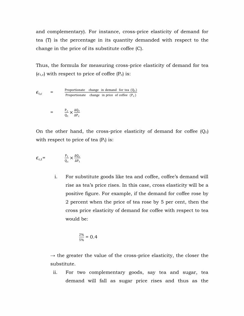
Thus, the formula for measuring cross-price elasticity of demand for tea
(𝜖t,c) with respect to price of coffee (Pc) is:
𝜖t,c = Proportionate change in demand for tea (Q t )
Proportionate change in price of coffee (Pc )
= Pc
Q t×
∆Q t
∆Pc
On the other hand, the cross-price elasticity of demand for coffee (Qc)
with respect to price of tea (Pt) is:
𝜖c,t= Pt
Qc×
∆Qc
∆Pt
i. For substitute goods like tea and coffee, coffee‟s demand will
rise as tea‟s price rises. In this case, cross elasticity will be a
positive figure. For example, if the demand for coffee rose by
2 percent when the price of tea rose by 5 per cent, then the
cross price elasticity of demand for coffee with respect to tea
would be:
2%
5% = 0.4
→ the greater the value of the cross-price elasticity, the closer the
substitute.
ii. For two complementary goods, say tea and sugar, tea
demand will fall as sugar price rises and thus as the

quantity of sugar demanded falls. In this case, cross price
elasticity of demand will be a negative figure. For example, if
a 4% rise in the price of sugar led to a 2% percent fall in
demand for tea, the cross elasticity of demand for tea with
respect to sugar would be:
2%
4% = - 0.5
→ the greater the value of negative cross-price elasticity, the higher
the degree of complementarity.

Some applications of cross-price elasticity For a given firm knowing the cross-price elasticity
of demand for its product is important during production plan. The firm must know the cross price elasticity of demand for their product when considering the effect on the demand for their product of a change in the price of rival’s product (substitute) or of a complementary good.
The other important application of this concept is
international trade. A nation must address the question, how does a change in the price of domestic goods affect the demand for imports? In most of the cases, if there is a high cross elasticity of demand for imports, and if prices at home rise due to inflation or other reasons, the demand for imports will rise substantially, and this will have a negative impact on the nation’s trade balance.

3.4 Income elasticity of demand
Apart from price of a product and related goods, another important
determinant of demand for a product is consumer‟s income. Thus,
income elasticity of demand (Y𝜖D) measures the responsiveness of
demand to a change in consumer incomes (Y). This measurement helps
us to predict how much the demand curve will shift for a given change in
income.
As you recall from earlier discussions, we said that, the relationship
between demand for normal goods and consumer‟s income is of positive
nature, unlike the negative price – demand relationship. That is, the
demand for normal goods and services increases with increase in
consumer‟s income and vice versa.
The formula for income-elasticity of demand for a product is: the
percentage (or proportionate) change in demand divided by the
percentage (or proportionate) change in income.
Y𝜖D = % ∆ QD
% ∆ Y
Thus, if a 2 percent rise in income caused a 5 percent rise in a product‟s
demand, then its income elasticity of demand would be:
5%
2% = 2.5
The major determinant of income elasticity of demand is the degree of
„necessity‟ of the good. When an economy develops, like the case for
developed countries, the demand for luxury goods expands rapidly as

people‟s incomes rise, whereas the demand for basic goods rises only a
little.
For instance, in most cases demand for vehicles, recreation and
entertainment have a high income elasticity of demand, whereas
items like vegetables have a low income elasticity of demand.
The other fact is, demand for some goods decreases as people‟s incomes
rise beyond a certain level. These are inferior goods. As people earn more,
they switch to a better quality of such inferior goods.

Some applications of income-elasticity The concept of income-elasticity can be used to
estimate future demand provided the rate of increase in income and income-elasticity of demand for the products are known. – Useful for firms in forecasting demand when changes in personal incomes are expected, holding other things constant.
It also can be used to define the ‘normal and ‘inferior’ goods. The goods whose income-elasticity is positive for all levels of income are termed as ‘normal goods’. On the other hand, the goods for which income elasticities are negative, beyond a certain level of income, are termed as ‘inferior goods’.

Unit Summary Elasticity describes the responsiveness of demand to changes in
price, income or other variables.
The value of the elasticity measure tells us whether the change is
elastic, unitary elastic or inelastic.
Number and closeness of substitute goods, nature of the
commodity, proportion of income spent on the good and time are
the major determinant factors of price elasticity of demand.
The cross-price elasticity of demand measures the responsiveness
of the demand for a good to changes in the price of a related good –
substitute or complementary good.
For substitute goods, demand will rise as price rises; but for
complementary goods demand will decrease as price rises.
Unit Review Questions 1. In a given demand curve there are different elasticity values
between different points. Explain.
2. Give an example of a good or a service that you know will have
totally elastic or infinitely inelastic demand nature.
3. Given the demand function Q= 30 – 2P,
(a) Calculate the elasticity and interpret the result for the fall in
price from 6 to 4
(b) Calculate the elasticity and interpret the result for the increase
in price from 8 to 10

Unit Four
Theory of Consumer Behavior
Introduction
This unit illustrates basic tools to understand the behavior of individuals
as consumers and the impact of alternative incentives on their decision.
The major focus will be on understanding how consumers behave in
market place. Again we use unit two‟s discussion of demand theory to
further analyze how a consumer decides how much of a good to buy at a
given price and why he/she buys more/less of a good when the price
changes. In general, you will understand how consumers respond to the
alternative choices that confront them.
Upon completion of this unit you will be able to
Discuss the different approaches to consumer behavior analysis.
Familiarize yourselves to different measurements of consumer
satisfaction (utility).
Understand and discuss consumer equilibrium in terms of utility
and indifference curve analysis.

4.1 Consumer Behavior
A consumer is an individual who purchases goods and services from
firms for the purpose of consumption. And, consumer behavior is about
how consumers decide on the basket of goods and services they
consume. It is essentially a decision-making behavior.
4.1.1 Approaches to consumer behavior analysis
We begin with an important axiom (assumption) that a consumer is a
utility maximizing entity. As a utility maximizing entity, the consumer
buys goods and services in such a way that he will generate maximum
utility from consumption. Utility refers to the power or property of a
commodity to satisfy human needs – a feeling of pleasure or a feeling of
satisfaction. A consumer who attempts to get the best value for the
money from his or her purchases is referred by economists as a rational
consumer.
4.1.2 Measuring utility
The question of measurability of utility is not a resolved concept among
economists. In one hand, economists hold that utility is quantitatively
measurable in absolute terms like weight and height of a person. On the
other hand, other groups of economists hold that utility is only ordinal
measurement – like high, higher, highest etc.
For our discussion we will ignore this unresolved problem and assume
that a person‟s utility can be measured in utils, where a util is one unit of
satisfaction.
4.2 Total and marginal utility

In order to understand more on the concept of utility we need to look at
the distinction between total utility and marginal utility.
4.2.1 Total utility (TU)
Total utility from a single commodity, may be defined as the sum of the
satisfaction derived from all the units consumed of the commodity within
a given time period. If a consumer consumes 4 units of apple a day, her
daily total utility from apple would be the satisfaction derived from those
apples. That is:
TU = U1 + U2 + U3 + U4
If she consumes n units, then total utility (TU) from n units is expressed
as:
TU𝑛 = U1 + U2 + U3 + … + U𝑛
And in case the number of commodities consumed is greater than one:
TU = Ua + Ub + Uc + … + U𝑛
Where subscripts a, b, c and n represent the consumption of different
commodities in a given period, say within a day.
4.2.2 Marginal utility (MU)
The marginal utility is the additional satisfaction gained from consuming
one extra unit within a given period of time. Thus from our example, we
might refer to the marginal utility that the consumer gains from her
second or fourth apple within a day.

→ Marginal utility is the change in the total utility resulting from
the change in the consumption. That is:
MU = ∆ TU
∆ C
Where ∆ TU = change in total utility, and ∆ C = change in consumption
Marginal utility (MU) can be also expressed as:
MU = MUn – (MUn−1)
4.3Law of diminishing marginal utility
This law states that as the quantity consumed of a commodity increase,
over a unit of time, the utility derived by the consumer from the successive
units goes on decreasing. Up to a certain level, the more of a commodity a
consumer consumes, the greater will be the total utility. However, as one
becomes more satisfied, each extra unit that the consumer consumes
will probably give a lesser additional utility than previous units. –
marginal utility falls, the more we consume a commodity within a given
time period.
For example, the second apple gives the consumer less additional
satisfaction than the first. The third and the fourth give less satisfaction
still. At some level of consumption, consumers‟ total utility will be at a
maximum. It will become hard to generate extra satisfaction by
consuming of further units within a given period of time. The sixth or
seventh unit of eating apple within an hour may result in zero marginal
utility. The tenth or eleventh unit of apple may give displeasure –
negative marginal utility.

The next table represents a numerical illustration of the law of
diminishing marginal utility. As you can see from the table, total utility
increases with increased in consumption of sausage, but at a decreasing
rate. This means, marginal utility decreases with increase in
consumption.
Table 4.1 Consumer‟s utility from consuming sausages per day
Units of sausage
consumed TU in utils MU in utils
0 0 0 – 0 = 0
1 15 15 – 0 = 15
2 25 25 – 15 = 10
3 30 30 – 25 = 5
4 32 32 – 30 = 2
5 30 30 – 32 = - 2
6 20 20 – 30 = - 10
The law of diminishing marginal utility is graphically illustrated in figure
4.1 and 4.2. The total utility and marginal utility curves have been
obtained by plotting the data given in table 4.1 above.
Figure 4.1 Total utility curve for sausage consumption

Figure 4.2 Marginal utility curve for sausage consumption
Note the following points from the total and marginal utility curves.
TU
0
5
10
15
20
25
30
35
0 2 4 6 8
To
tal u
tili
ty
Sausage consumed per unit of time
MU
-15
-10
-5
0
5
10
15
20
0 1 2 3 4 5 6 7
Marg
inal u
tili
ty
Sausages consumed per unit of time

The MU curve slopes downwards. This is due to the law of
diminishing marginal utility.
The TU curve starts at the origin. Zero consumption yields zero
utility.
TU reaches a peak when MU is zero. MU can be derived from the
TU curve since, MU = ∆ TU
∆ C
4.4 Consumer Equilibrium
As we said earlier, a consumer is assumed as a utility maximizer. A
consumer reaches equilibrium position, when she maximizes her total
utility given her income and prices of commodities she consumes.
Considering the consumer‟s money (payment to the commodity) will help
us to resolve the problem of measuring utils that we mentioned earlier.
Measuring utility with money means, utility becomes the value that a
rational consumer places on her consumption.
Marginal utility therefore becomes the amount of money a consumer
would pay to obtain one more unit, that is, what the extra unit is worth
to the consumer. Generally, analyzing consumer‟s equilibrium requires
answering the question as to how a consumer allocates her money
income among the various goods and services she consumes.
4.4.1 Consumer equilibrium – one commodity case
A utility maximizing consumer reaches her equilibrium position when
allocation of her expenditure is such that the last Kwacha spent on each
commodity yields the same utility. How does the consumer reach this
position?

Suppose that a consumer with a given level of money income consumes
only one commodity, X. Both money income and commodity X have
utility for the consumer. She has an option of either spend her money
income on commodity X or retain it with her.
If marginal utility of commodity X ( MUx) is greater than marginal utility
of money income (MUm), total utility can be increased by exchanging
money for the commodity. Therefore, a utility maximizing consumer
exchanges his money income for the commodity as long as MUx> MUm.
But the money a consumer spent on commodity X is equal to price of X
multiply by quantity of X consumed, i.e. Px (X). In terms of marginal
utility, it is equal to Px (MUm). Therefore, the consumer will exchange her
money income for commodity X so long as:
MUx > Px (MUm )
The utility maximizing consumer reaches her equilibrium with the level
of her maximum satisfaction where:
MUx = Px (MUm )
Alternatively, the consumer reaches equilibrium where,
MUx
Px (MUm ) = 1
4.4.2 Consumer Equilibrium: the general case (multiple commodities)
In reality a consumer consumes a large number of goods. This means the
MU derived from different commodities differ widely. This is

because,some commodities yield higher utility and some lower. And, MU
of some goods decreases more rapidly than that of others.
A rational and utility maximizing consumer consumes commodities in
the order of their utilities. She picks up a commodity which yields the
highest utility followed by the commodity yielding the second highest
utility and so on. She allocates her expenditure from one commodity to
the other until she reaches a stage where M of each commodity is the
same per unit of expenditure.
For the moment suppose that the consumer only consumes two
commodities X and Y, their prices being Px and Py respectively. Thus, the
consumer allocates her income between commodities X and Y in such a
way that:
MUx = Px (MUm )
and MUy = Py (MUm )
or alternatively, consumer is in equilibrium where:
MU x
Px (MU m ) = 1 (1)
MU y
Py (MU m ) = 1 (2)
Equation (1) and (2) can be written together and equilibrium condition
will be:
MU x
Px (MU m ) = 1 =
MU y
Py (MU m )
Or MU x
MU y =
Px (MU m )
Py (MU m )

Or MU x
MU y =
Px
Py
Or MU x
Px =
MU y
Py
This last equation leads to the conclusion that the consumer reaches her
equilibrium when the marginal utility derived from each penny spent on
the two commodities X and Y is the same.
The two commodities case can be expanded for generalized consumer‟s
equilibrium. In reality a consumer consumes a number of goods and
services given her income and at given prices. Thus, consumer
equilibrium condition may be expressed as:
MU a
Pa =
MU b
Pb=
MU c
Pc = … =
MU z
Pz
→ A utility maximizing consumer intends to equalize to reach her
equilibrium position is not the marginal utility of each commodity she
consumes, but the marginal utility of each unit of her money expenditure
on various goods and services.
4.5 Indifference analysis
In the preceding discussion of marginal utility theory we assumed that
utility can be measured in absolute terms. Though the theory has a
strong foundation and logic in explaining consumer choice, it still has
limitation from the dimension of assigning values for utility. In reality it
is a difficult task to assign a value for the level of satisfaction a consumer
derived from consuming a commodity.
Economists developed an alternative approach which is called
indifference analysis. Unlike marginal analysis, the indifference analysis
does not involve measuring the amount of utility a consumer achieves,
but rather it ranks various combinations of goods in order of preference.
It is an expression of the consumer‟s preference for one commodity over
another or a basket of goods over another.
Two axioms (assumptions) on the concept of indifference analysis
i. The indifference analysis states that it is easy for the consumer to
which of any two goods she prefers than expressing her utility in
quantitative terms. That is, it is always possible for the customer
to say she prefers chocolate than ice-cream, or cheese burger than
sausage, or a shirt than sweater.
ii. Based on the facts from (1), the consumer can order all the
commodities she consumes in the order of their preference.
4.5.1 Indifference curve
Thus, we can define indifference curve as a curve that shows all the
various combinations of two goods that give equal amount of satisfaction
or utility to a consumer. Since a different combination of two goods gives
the same utility to the consumer, she is indifferent between two goods
when it comes to making a choice between them.
Let us consider the following example to clearly understand the meaning
of indifference curve. Suppose that after a quick survey for a consumer
choice of different combinations of orange and banana she prefers from a
supermarket, it is found that the following combinations of the two
commodities will give her same level of satisfaction.
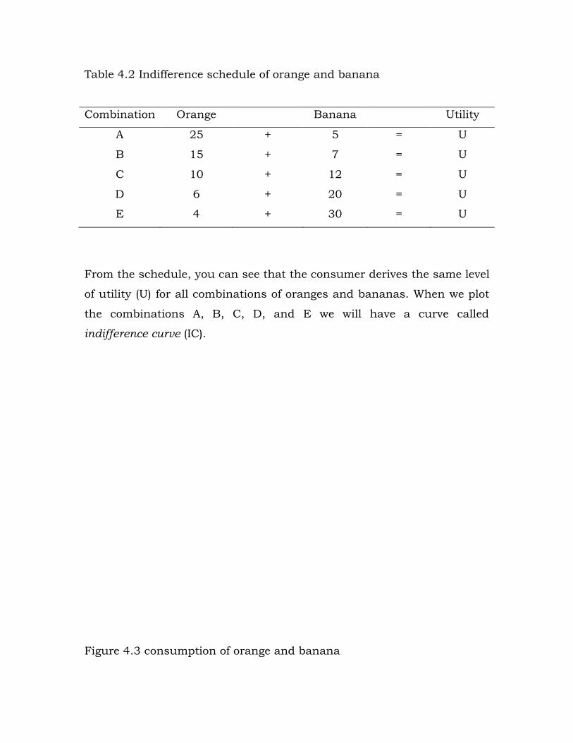
Table 4.2 Indifference schedule of orange and banana
Combination Orange Banana Utility
A 25 + 5 = U
B 15 + 7 = U
C 10 + 12 = U
D 6 + 20 = U
E 4 + 30 = U
From the schedule, you can see that the consumer derives the same level
of utility (U) for all combinations of oranges and bananas. When we plot
the combinations A, B, C, D, and E we will have a curve called
indifference curve (IC).
Figure 4.3 consumption of orange and banana

The indifference curve is a downward sloping and is convex (bowed in) to
the origin. This is due to the nature of different slope values along the IC.
The slope of the IC shows the rate at which the consumer is willing to
exchange one good to for the other for the same level of satisfaction. For
instance, a move from point A to point B means the consumer gives up
10 units of oranges and requires 2 units of bananas to compensate the
loss. Thus the slop of the IC is -10/2 = - 5.
Technically the slope of the IC is known as the marginal rate of
substitution (MRS). Ignoring the negative sign, the slope which is equal to
MRS for a move from point A to point B is 5.
The marginal rate of substitution decreases as we go down the curve
since the slope (steepness of the curve) gets less and less. For instance, a
move from point C to point D will result in MRS = 0.5. The MRS
diminishes because as a consumer give up orange for banana the stock
A
B
C
D
E
0
5
10
15
20
25
30
0 10 20 30 40
Banana
Ora
ng
e

of banana increases and that of orange decreases. This means it will
become difficult for the consumer to sacrifice more units of orange for a
given amount of banana.
4.5.2 Marginal Rate of Substitution and Marginal Utility
When a consumer moves from point A to point B she remains at the
same level of satisfaction with different combinations of orange and
banana. In other words the utility sacrificed by giving up 10 oranges
must be equal to the utility gained by consuming 2 more oranges. This
means, at this point of exchange, the marginal utility of a banana must
be five times as great as that of an orange.
Therefore, MUbanana / MUorange = 5. And this is equal to the marginal rate
of substitution. In general, for two goods X and Y with X plotted on the
horizontal axis and Y on the vertical axis, then:
MRS = MU x
MU y = slope of indifference curve
4.5.3 Indifference map
The consumer can have more than one indifference curves. Our
consumer can show another set of combinations of oranges and bananas
that all give her a higher (but equal) level of utility than the case we had
in table 4.2. Indifference curves further out to the right would show
combinations of the two goods that yield a higher utility, and curves
further into the left would show combinations yielding a lower utility.
Figure 4.4 Indifference map

IC3
Properties of Indifference curves
i. Indifference curves have a negative slope
ii. Indifference curves are convex to the origin
iii. Indifference curves do not intersect
iv. Between any two indifference curves the upper one implies a
higher level of satisfaction than the lower.
4.6 The budget constraint and the budget line
A utility maximizing consumer would prefer to reach the highest possible
indifference curve on her indifference map. But in reality the consumer
has a limited income. Limited income sets a limit to which a consumer
can maximize her utility.
The limitedness of income acts as a constraint on the utility maximizing
behavior of the consumer. This is known as the budget constraint.
Assuming a two commodity model, the budget constraint can be written
as:
Px × Qx + Py × Qy = M (3)
IC1
IC2
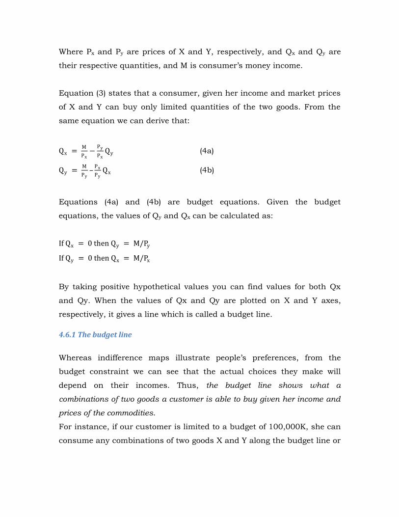
Where Px and Py are prices of X and Y, respectively, and Qx and Qy are
their respective quantities, and M is consumer‟s money income.
Equation (3) states that a consumer, given her income and market prices
of X and Y can buy only limited quantities of the two goods. From the
same equation we can derive that:
Qx = M
Px−
Py
PxQy (4a)
Qy = M
Py–
Px
PyQx (4b)
Equations (4a) and (4b) are budget equations. Given the budget
equations, the values of Qy and Qx can be calculated as:
If Qx = 0 then Qy = M/Py
If Qy = 0 then Qx = M/Px
By taking positive hypothetical values you can find values for both Qx
and Qy. When the values of Qx and Qy are plotted on X and Y axes,
respectively, it gives a line which is called a budget line.
4.6.1 The budget line
Whereas indifference maps illustrate people‟s preferences, from the
budget constraint we can see that the actual choices they make will
depend on their incomes. Thus, the budget line shows what a
combinations of two goods a customer is able to buy given her income and
prices of the commodities.
For instance, if our customer is limited to a budget of 100,000K, she can
consume any combinations of two goods X and Y along the budget line or

inside it (feasible area). She cannot afford to buy combinations that lie
outside it, the infeasible region for the given budget.
4.6.2 Shift in budget line
The budget line will shift inward or outward either due to change in
consumer‟s income or prices of the commodities.
If the consumer‟s income (hence budget) increases, the budget line
will shift outwards, but parallel to the old budget line. Assume the
consumer now has 150,000K but no change in the prices of X and
Y. This means the consumer can buy more now than the previous
period.
If income remaining (hence budget) the same, change in price
changes the position of the budget line. Assume prices of both
goods decline by 25%. This will cause an increase in the
purchasing power of the consumer.

Figure 4.5 Budget line
4.7 Equilibrium of the consumer
Now we developed the necessary tools of consumer analysis, and at this
level we can set the model for consumer‟s equilibrium. A consumer
attains her equilibrium when she eventually maximizes her total utility,
given her income and market prices of goods and services she consumes.
Technically, there are two conditions of consumer equilibrium:
i. Necessary condition
ii. Supplementary condition
The necessary condition of maximum satisfaction is that MRS must be
equal to the ratio of commodity prices. That is:
d
c
b
a
0
5
10
15
20
25
30
35
0 5 10 15 20
Un
it o
f g
oo
d Y
Unit of good X

MRSx,y = MUx
MUy =
Px
Py
Furthermore, the supplementary condition must be fulfilled at the
highest possible indifference curve.
Slope = ∆Y
∆X =
MUx
MUy =
Px
Py
Graphically consumer‟s equilibrium has been shown in fig … indifference
curves IC1, IC2 and IC3 represent indifference map of the consumer and
his budget line is given by the line AB. As you can see the budget line AB
is tangent to IC2 at point E. this point fulfills both the necessary and
supplementary conditions.
At point E the slopes of the indifference curve IC2 and the budget
line (AB) are equal. This fulfills the first order condition. That is,
the slope of the indifference curve: ∆Y
∆X =
MU x
MU y = MRSy,x ;
And the slope of the budget line is OA
OB =
Px
Py
Thus, at point E MRSy,x =Px
Py
The tangency of IC2 with the budget line, AB, indicates that IC2 is
the highest possible indifference curve which the consumer can
reach given her budget constraint and prices of the goods.

Figure 4.6 Consumer‟s Equilibrium
A
B
IC2 IC3
IC1

Some applications of indifference curve analysis Even if the indifference curve analysis has a number of limitations to apply to the real world economic problems, it has been used to analyze: Different government policies like taxation,
subsidy and rationing policies Gains from exchange of goods between individuals,
sectors and countries Derivation of labor supply curve International trade and welfare economics
Unit Summary A consumer buys goods and services in order to consume and
generate maximum utility.
Utility refers to a feeling of pleasure or a feeling of satisfaction.
Total utility from a single commodity, may be defined as the sum of
the satisfaction derived from all the units consumed of the
commodity within a given time period.
The law of diminishing returns states that as the quantity
consumed of a commodity increases, over a unit of time, the utility
derived by the consumer from the successive units goes on
decreasing.
Indifference analysis ranks various combinations of goods in order
of the consumer‟s preference.

Unit Review 1. Why does the marginal rate of substitution (MRS) diminish along
the indifference curve?
2. Using an indifference curve explain how the consumer equilibrium
is affected by a change in the consumer‟s income?
3. Explain why an MRS between two goods must equal the ratio of
the price of the goods for the consumer to achieve maximum
satisfaction?
4. Assume consumers in Lusaka pay twice as much for good X as
they do for good Y. However, goods X and Y have the same price in
Kabwe. If consumers in both towns maximize utility, will the
marginal rate of substitution of Y for X be the same for consumers
in both towns? If not, which is higher?

Unit Five
Theory of the Firm Production
Introduction
In this unit you will extend your knowledge of the theory of supply.
Supply is a result of production. Thus, in this chapter we will discuss the
different tools of production analysis, which are essential for
understanding the theory of production. You will further understand the
basic relationships between inputs (factors of production) and outputs
(the level of production).
Upon completion of this unit you should be able to answer the following
questions.
What combination of inputs will be used for producing a given
good?
What is the most efficient combination of inputs?
What are the conditions for optimum level of production and firm‟s
equilibrium?
What determines costs and revenue?
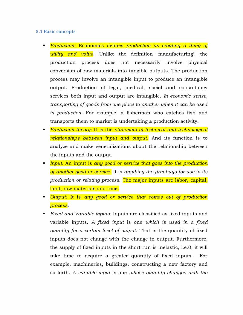
5.1 Basic concepts
Production: Economics defines production as creating a thing of
utility and value. Unlike the definition „manufacturing‟, the
production process does not necessarily involve physical
conversion of raw materials into tangible outputs. The production
process may involve an intangible input to produce an intangible
output. Production of legal, medical, social and consultancy
services both input and output are intangible. In economic sense,
transporting of goods from one place to another when it can be used
is production. For example, a fisherman who catches fish and
transports them to market is undertaking a production activity.
Production theory: It is the statement of technical and technological
relationships between input and output. And its function is to
analyze and make generalizations about the relationship between
the inputs and the output.
Input: An input is any good or service that goes into the production
of another good or service. It is anything the firm buys for use in its
production or relating process. The major inputs are labor, capital,
land, raw materials and time.
Output: It is any good or service that comes out of production
process.
Fixed and Variable inputs: Inputs are classified as fixed inputs and
variable inputs. A fixed input is one which is used in a fixed
quantity for a certain level of output. That is the quantity of fixed
inputs does not change with the change in output. Furthermore,
the supply of fixed inputs in the short run is inelastic, i.e.0, it will
take time to acquire a greater quantity of fixed inputs. For
example, machineries, buildings, constructing a new factory and
so forth. A variable input is one whose quantity changes with the

change in output, example, labor and raw materials. In short run,
the supply of variable input is elastic.
Short run and long run: In relation to variable and fixed inputs, we
also use two distinctions viz., short run and long run. The short-
run refers to a period of time in which the supply of certain inputs-
like buildings and machines are fixed or inelastic. Therefore, in the
short-run, production of a commodity can be increased only by
using more of variable inputs such as labor and raw materials. The
long-run refers to a period of time in which the supplies of all the
inputs are variable. That is, the supply response is elastic. That is,
in the long-run, availability of even the fixed factors increases. In
the long-run, therefore, production of a commodity can be
increased by using more of both, variable and fixed inputs.
Total, marginal and average product: In simple term total product
means total output at a given period of time. On the other hand,
marginal product is the marginal (last unit) addition to the total
output due to marginal (last unit) addition of a variable input.
It can be expressed as:
MP = ∆𝑄
∆𝐹𝑉
Where, ∆𝑄= change in total output, and ∆𝐹𝑉 = change in both fixed and
variable inputs. Assuming labor as the variable input, the marginal
product of labor (MPL ) is defined as change in output (Q) resulting from
change in labor employed. Thus,
MPL =∆𝑄
∆𝐿

Average product of labor can be defined as:
APL = 𝑄
𝐿
5.2 Production function
Production function shows us the relationship between inputs and
outputs. To illustrate the algebraic form of production function, let us
suppose that a copper mining employs only two inputs, i.e., capital (k)
and labor (L) in its copper production activity. The production function
could be:
Q = f K, L
Where Q = the quantity of copper produced per time unit, K = capital,
and L = labor.
The production function states that the quantity of copper produced is
the function of or depends on the quantity of capital (K) and labor (L)
used. It also implies the maximum quantity of copper that can be
produced given the total volume of capital and total number of workers
employed. Increasing copper production will require increase in the
inputs of K and L.
By definition (for simplicity) we said supply of capital is inelastic in the
short-run and elastic in the long-run. In the short-run, therefore, the firm
can increase copper production only by increasing labor, since the
supply of capital in the short run is fixed. In the long-run, however, the
firm can employ more of both capital and labor. Accordingly, the firm

would have two types of production function, i.e., short-run production
function and long-run production function.
5.2.1 Short-run production function
For an industry as a whole production is more of a function of variable
inputs, like labor, in the short-run. For the supply of capital is fixed and
inelastic in the short-run. The production can be increased by employing
more of the variable inputs.
The Laws of Diminishing Returns
When production is carried out with a given variable input factor and a
fixed amount of a fixed factor, the total output may increase first at
increasing rates, then at constant rates and eventually at a diminishing
rate. This relationship between the variable factor and the output is
called the Law of Diminishing Return.
In our example of copper production, the law can be stated as follows. As
more and more units of variable input, labor, is employed, with capital
held constant, the successive unit of labor may at first yield an
increasing return but will eventually yield diminishing returns. The total
output initially increase at increasing rates then increase at a decreasing
rate, remains constant or eventually even decrease.
To illustrate the Law of Diminishing Returns, let us assume that the
copper mining firm possess a set of mining machinery as its capital (K)
which is fixed in the short-run and that it can increase only the number
of mine workers to increase its copper production. Thus, the short-run
production function for the firm will be of the form

Q = f (L)
And also assume that the labor-output relationship is given as:
Q = -L3 + 10L2 + 20L
Given this production function, you can substitute different numerical
values for L in the function and generate a series of maximum quantity
of copper (Q) that can be produced with different number of workers. For
example, if we substitute 3 for L, the production function will be:
Q = -33 + 10 x 52 + 20 x 5 =123
Table 5.1 Production with one variable input
No of workers
(L)
Total output
(Q)
(tones)
Marginal
product
(MPL)
Average
product
(APL)
Stage
1 29 29 29
I 2 72 43 36
3 123 51 41
4 176 53 44
5 225 49 45
II 6 264 39 44
7 287 23 41
8 288 1 36
9 261 -27 29 III
10 200 -61 20
Where MPL= ∆Q/∆L; APL = Q/L

Table 5.1 shows array of output levels associated with different number
of workers 1 – 10 in copper production. From the total output we drive
the marginal product (MPL) and the average product (APL) of labor.
The information in the above table can be presented graphically as
follows.
Figure 5.1 Total product, average product and marginal product curves
TP
MPL
APL
-100
-50
0
50
100
150
200
250
300
350
0 2 4 6 8 10 12
To
tal o
utp
ut (t
on
es)
No. of workers

Table 5.1 and figure 5.1 present the three general stages in the operation
of the law of diminishing returns. In stage I, MPL continues to increase
making TPL increase at an increasing rate. In stage II, MPL starts falling
as TPL increases at a decreasing rate. In stage III, MPL becomes negative
and TPL starts falling. The reasons for increasing, and diminishing
returns are given as follows.
Stage I – Increasing Returns
Initially, given the fixed factor which is indivisible, a certain minimum
labor is required to make the optimum use of capital. If a smaller
number of workers are used, capital remains underutilized. When more
and more units of labor are used, capital gets more and more fully
utilized. It increases productivity of both labor and capital. This shows
the Law of Increasing Returns to Scale.
Stage II Diminishing Returns
A continuous increase of more and more labor after a certain point
means, workers get less and less capital to work with. As a result,
marginal productivity of labor decreases.
Stage III – Negative Returns
Technically employing more labor beyond the optimum capital-labor
combination means substitution of labor for capital. But there is limit to
which one factor can substitute another. The limit in our case is when
MPL = 0. Any addition of labor beyond this limit leads to overcrowding
and lower availability of tools and equipments which cause a fall in total
production.

5.2.2 The Long-run Production Function
We have seen the short-run production function in which one input,
labor, is variable, and the other, capital, is fixed. Now let us see the case
for long-run, for which both labor and capital are variable. The firm can
now produce its output in a variety of ways by combining different
amounts of labor and capital.Now, let us see the input-output
relationships under the condition that all the inputs (labor and capital)
are changed proportionately and simultaneously.
Isoquant
Let us examine the production function (technology) of a firm that uses
two inputs and can vary both inputs. Suppose the inputs are labor and
capital to produce copper. Below, the table shows the output achievable
for various combinations of inputs.
Table 5.2 Production of 50 tones of copper with two variable inputs
Alternative combinations (techniques) A B C D E
Labor 5 12 20 30 50
Captital 40 20 10 6 4
From the schedule, a firm can combine various units of capital and labor
to produce 50 tones of copper per week. For instance alternative A is a
capital-intensive technique, using 40 units of capital and only 5 workers.
As we move towards technique E, labor is substituted for capital. The
techniques become more labor intensive.

Figure 5.2 Isoquant curve
0
5
10
15
20
25
30
35
40
45
0 10 20 30 40 50 60
Cap
ital
Labor

The information in table 5.2 is presented graphically in figure 5.2. The
resulting curve is called Isoquant curve. An isoquant is a curve that
shows all the possible combinations of inputs that yield the same output.
Isoquant shows the flexibility that firms have when making production
decisions. Firms can obtain a particular level of output by substituting
one input for another.
Isoquant map
When a group of isoquants are combined in a single graph, this is called
an isoquant map. Figure 5.3 shows an isoquant map. An isoquant map is
another way of descriing a production function, just as an indifference
map is a way of describing a utility function.
Figure 5.3 Isoquant map

5.3 Optimal Combination of Inputs
Given the technology, a given output can be produced with different
input combinations. With two inputs, the slope of each isoquant
indicates how the quantity of one input can be traded off against the
quantity of the other, while output is held constant.
Ignoring the negative sign of the curve, we call the slope the marginal
rate of technical substitution (MRTS). The marginal rate of technical
substitution of labor for capital is the amount by which the input of
capital can be reduced when one extra unit of labor is used, so that the
output remains constant.
MRTS = - change in capital input/ change in labor input
= - ∆K/∆L for a fixed level of output.
Diminishing MRTS
The diminishing MRTS tells us that the productivity of any one input is
limited. As more and more labor is added to the production process in
place of capital, the productivity of labor falls. Similarly, when more
capital is added in place of labor, the productivity of capital falls. Efficient
production requires a balanced mix of both inputs.
Generally we can say MRTS is closely related to the marginal products of
labor MPL and capital MPK. Thus, the additional output resulting from
the increased labor input is equal to the additional output per unit of
additional labor (the marginal product of labor) times the number of
units of additional labor.
Additional output from increased use of labor = (MPL) (∆L)

Similarly, the decrease in output resulting from the reduction in capital
is the loss of output per unit reduction in capital (the marginal product
of capital) times the number of units of capital reduction.
Reduction in output from decreased use of capital = (MPK) (∆K)
In order to keep output constant by moving along an isoquant, the total
change in output must be zero. That is,
(MPL) (∆L) + (MPK) (∆K) = 0
Rearranging terms finally will give us
(MPL)/(MPK) = - (∆K/∆L) = MRTS
This final equation tells us that the marginal rate of technical substitution
between two inputs is equal to the ratio of the marginal products of the
inputs.
5.4 Returns to Scale
When all the inputs change proportionately, the scale of production (size
of firm) will change. The laws that exist to the input-output relationships
under the condition of changing scale of production are called the Laws
of Returns to Scale.
There are three laws of returns to scale. These are;
I. Increasing returns to scale: This happens when the rate of increase
in output is more than proportional to the increase in inputs and if
rate of increase goes on increasing with subsequent increase in
inputs. For example if inputs increase by 50% and output

increases by more than 50%, say 60%, it is an increasing returns
to scale.
II. Constant returns to scale: This is the case when increase in output
is proportional to increase in inputs. For example if inputs doubled
and output is also doubled, then the return to scale is constant.
III. Decreasing returns to scale: This happens when the rate of increase
in output is less than proportional to the increase inputs and it
goes on decreasing with subsequent increase in inputs. That is,
when inputs are doubled, output is less than doubled and so on.
Causes of Increasing, Constant and Diminishing returns to scale
(i) The returns to scale increase are because of economies of scale. A firm
experiences economies of scale if cost per unit of output falls as the scale
of production increases. At least three kinds of economies to scale make
plausible reasons for increasing returns to scale.
Technical and managerial indivisibilities: Certain inputs,
particularly mechanical equipment and managerial skills used in
the process of production are available in a given size. For
instance consider a combine harvester. A small scale farmer could
not make full use of one. There is not as such half combine
harvester, half tractor or hiring half a manager. Because of their
indivisibility, such factors have to be employed in a minimum
quantity even if scale of production is much less than their
capacity output. Thus, when scale of production is increased by
increasing all inputs, the productivity of indivisible factors
increases exponentially. This results in increasing returns to
scale.
Specialization and division of labor: Higher degree of specialization
can be achieved both from labor and machinery, which becomes

possible with increase in scale of production. The use of
specialized labor and machinery increases productivity per unit of
inputs. Their cumulative effects contribute to the increasing
returns to scale. Furthermore, managerial specialization
contributes a great deal in increasing production.
The ‘dimensional’ and ‘container’ principle: Increasing returns
could be a matter of dimensional returns. For example, when the
size of a room (15m x 10m = 150sq.mt) is doubled to 30mt x 20mt,
the area of the room is more than doubled, i.e., 30mt x 20mt =
600sq.mt. Furthermore, increasing returns can come from capital
equipment that contain things like oil tankers, pipes etc. When
the diameter of a pipe is doubled, the flow of water is more than
doubled.
(ii) The constant returns to scale attributes to the limits of the
economies of scale. With the expansion in the scale of production,
economies arise from such factors as indivisibility of certain factors,
greater possibility of specialization of capital and labor, use of labor-
saving techniques of production, etc. But there is a limit to the
economies of scale. When economies of scale disappear and
diseconomies are yet to begin, the returns to scale become constant.
The diseconomies arise mainly because of decreasing efficiency of
management and scarcity of certain inputs.
(iii) The decreasing returns to scale attribute to diseconomies of scale.
When firms get beyond a certain size, costs per unit of output may
start to increase. The reasons for diseconomies of scale are:
Management capacity of coordination may decrease as the firm
becomes larger and more complex, and as lines of
communication get longer.

Jobs become boring and repetitive for workers and they feel as
if they are insignificantly small part of a large organization.
Limitedness and exhaustibility of some factor inputs (natural
resources) leads to reduction of production.
Unit Summary Production function shows the relationship between inputs and
outputs. The law of diminishing returns states that, as more and
more units of variable input are employed while holding the fixed
input, the successive unit of variable input may at first yield an
increasing return and eventually yield diminishing returns.
An isoquant curve shows all the possible combinations of inputs
that yield the same output. The slope of an isoquant indicates how
the quantity of one input can be traded off against the quantity of
the other, while output is held constant.

The marginal rate of technical substitution (MRTS) of two inputs is
the amount by which one input can be reduced while using one
extra unit of the other input, so that the output remains constant.
Increasing returns to scale happens when the rate of increase in
output is more than proportional to the increase in inputs and if
rate of increase goes on increasing with subsequent increase in
inputs.
A constant return to scale is the case when increase in output is
proportional to increase in inputs.
Decreasing returns to scale happens when the rate of increase in
output is less than proportional to the increase inputs and it goes
on decreasing with subsequent increase in inputs.
The increasing return to scale is largely because of economies of
scale; the constant returns to scale attributes to the limits of the
economies of scale; and the decreasing returns to scale attribute to
diseconomies of scale.
Unit Review Questions 1. In order to keep output constant by moving along an isoquant, the
total change in output due to changes in one of the inputs must be
zero. Explain?
2. How does a short-run production function differ from the long-run
production function?
3. Why do firms experience diminishing returns for labor in the short-
run production?
4. Interpret the result MRTS of labor to capital = 3

5. Why does the MRTS decline as a firm continuously substitutes
labor for capital?
6. What kinds of returns to scale does a firm experience with the
following production functions?
(a) Q = 2L + 3K
(b) Q = 2L1/2 + 2K
(c) Q = L2 + 3L
Unit Six
Theory of the Firm’s Cost
Introduction

In the previous unit we stated the theory of production in terms of
physical quantities, like, labor as number of workers, capital as units of
machinery and output as measures of some unites e.g., tones of copper.
However, most decisions regarding price and production are taken on the
basis of money value of input and output rather than their physical
quantities. Thus, in this chapter we will discuss the relationship between
the output and cost of production.
Upon completion of this unit you should be able to
Identify the different types of firm‟s costs and how a firm‟s cost is
classified in terms of production time/technology.
Calculate and understand the different expressions of the firm
costs.
Discuss the relationship among certain cost expressions.
6.1 Basic concepts

Actual costs/ Accounting costs: are costs which are actually incurred by
the firm in the payment for labor, material, building, machinery, etc. The
total money expenses recorded in the books of accounts are the actual
costs. Generally it is the sum of actual expenses and depreciation
expenses for capital equipment.
Opportunity cost/ Economic cost: is the cost associated with opportunities
that are forgone by not using the firm‟s resources to their second best
alternative use. Alternatively, the opportunity cost equals the expected
returns from the second best use of the resources forgone to avail the
gains of their best use.
Fixed costs (FC): Are costs that are paid by a firm that is operating,
regardless of the level of output it produces. It is a cost that does not
vary over a certain level of output. Fixed costs include cost of (i)
managerial and administrative staff; (ii) depreciation of machinery,
building and other fixed assets; and (iii) maintenance of land, etc. The
concept of fixed cost is associated with short-run production periods.
Variable costs (VC): Are those which vary with the variation in the total
output. Variable costs are functions of the output. Variable costs include
cost of raw materials, running cost of fixed capital, direct labor cost
associated with the level of output, and the costs of all other inputs that
vary with output.
Total cost (TC): represents the value of the total resources used in the
production of goods and services. It refers to the total outlays of money
expenditure, on the resources used to produce a given output. It is
derived from the cost function for a given output.
TC = FC + VC

Average total cost (ATC): It is a result of mathematical operation than
being an actual cost. It is obtained by dividing the total cost (TC) by the
total output (Q).
ATC = TC/Q
ATC is classified into Average Fixed Cost (AFC = FC/Q) and Average
Variable Cost (AVC = VC/Q).
Marginal cost (MC): It is the addition to the total cost on account of
producing one additional unit of the product. Sometimes it is called
incremental cost. Because fixed cost does not change as the firm‟s level
of output changes (at least in the short-run), marginal cost is equal to
the increase in variable cost.
MC = ∆TC/∆Q = ∆VC/∆Q
Marginal cost tells us how much it will cost to expand output by one unit.
Short-run costs: Are the costs which vary with the variation of output, the
size of the firm remaining the same. In other words, short-run costs are
the same as variable cost.
Long-run costs: Are costs which are incurred on fixed assets, like building
and machinery. Long run costs are fixed costs. But, in the long-run even
the fixed costs become variable costs as the size of the firm or scale of
production increases.
Consider the following example for further understanding of how we can
calculate the different types of costs in the short-run given fixed and
variable costs for different levels of output. The total cost figures TFC and
TVC are given. Check by yourself how the TC, AFC, AVC, AC and MC
values are derived by using their respective definitions.

Table 6.1 Total, Average and Marginal Costs
Output
(Q)
Total costs Average and marginal costs
TFC TVC TC AFC AVC AC MC
1 50 30 80 50 30 80 80
2 50 50 100 25 25 50 20
3 50 60 110 17 20 37 10
4 50 65 115 12 16 29 5
5 50 75 125 10 15 25 10
6 50 100 150 8 17 25 25
7 50 145 195 7 21 28 45
8 50 225 275 6 28 34 80
6.2 Cost in the Short-run
The short-run total cost is composed of two major elements – total fixed
cost and total variable cost. That is,
TC = TFC + TVC
TFC remains fixed in the short-run, for a certain level of output, whereas
TVC varies with the variation in output. Any change in the short-run is
only attributable to changes in the variable costs. Thus,
∆TC = ∆TFC + ∆TVC, and in the short-run, ∆TFC = 0
∆TC = ∆TVC = MC why?
6.2.1 Output and Average and Marginal costs relations
As you can see from table 6.1,

Average fixed cost (AFC = TFC/Q) decreases throughout as output
increases, because TFC remains constant while Q increases.
Average variable cost (AVC = TVC/Q) first decreases and then
increases. This is because while output increases at a constant
rate of 1, TVC increases first at a diminishing rate then at an
increasing rate.
The Average cost (AC = TC/Q) first decrease till Q = 5, and then
begins to increase. AC falls over some level of output because of
increasing returns to the variable input. This property of cost-
output relations makes the AC curve U-shaped.
The marginal cost (MC = ∆TC/∆Q) decreases till certain level of
output (e.g., Q = 4), and then begins to rise at an increasing rate.
Given the TFC, the fall and rise in MC is determined by the
changes in TVC (i.e., ∆TVC). For, ∆TC is determined by ∆TVC.
6.2.2 Short-run cost curves
Below, figures 6.1 and 6.2 illustrate how various cost measures change
as output changes. Figure 6.1 shows the relationship between output
and TFC, TVC and TC. The TFC remains fixed for the whole range of
output, and takes the form of straight horizontal line. The TVC curve
shows that the total variable cost first increases at a decreasing rate and
then, at an increasing rate with the increase in the total output. The
pattern of change in TVC comes from the law of increasing and
diminishing returns to variable inputs.

Figure 6.1 Total cost, total variable cost and total fixed cost curves
Figure 6.2 clearly reflects the laws of returns to input in terms of cost of
production. In the initial stage of production, both AFC and AVC are
declining because of internal economies. Since AC = AFC + AVC, the AC
is also declining. This shows the operation of the law of increasing
returns. But beyond output of 5 units, while AFC continues to fall, AVC
starts increasing because of a faster marginal increase in the TVC.
The AC reaches its minimum when output increases from 4 to 5 units.
Beyond this level of output, AC starts increasing which shows the Law of
FC
VC
TC
0
50
100
150
200
250
300
0 1 2 3 4 5 6 7 8 9
Co
st
Output

Diminishing Returns coming into operation. The MC curve represents the
patterns of change in both the TVC and TC curves as output changes. A
downward trend in the MC shows increasing marginal productivity of the
variable input which is mainly because of internal economies resulting
from increase in production. Increase in the MC means no more internal
economies of the firm.
6.2 AFC, AVC, AC and MC curves
Relationship between AC and AVC
i. Since AC = AFC + AVC, AC falls so long as AFC and AVC fall.
ii. When AFC falls but AVC increases, change in AC depends on the
rate of change in AFC and AVC, on the following pattern:
If decrease in AFC > increase in AVC, AC falls;
AFC
AVC
AC
MC
0
10
20
30
40
50
60
70
80
90
0 1 2 3 4 5 6 7 8 9
Co
st
Output

If decrease in AFC = increase in AVC, AC remains constant;
and
If decrease in AFC < increase in AVC, AC begins to increase
Relationship between MC and AC
i. When MC falls, AC follows. But the rate of fall in MC is greater
than that of AC. For MC, the decreasing marginal cost is attributed
to a single marginal unit while, for AC, the decreasing marginal
cost is distributed over the whole output. As long as MC curve lies
below the AC curve, MC pulls AC downwards and when MC is
above AC, it pulls the latter upwards.
ii. When MC increases, AC also increases but at a lower rate for the
reason given above.
iii. MC intersects AC at its minimum point.
6.3 Cost in the Long-run
The major difference between the short-run and the long-run is that, in
the short-run some costs are fixed whereas in the long-run, all costs
become variable. Which means, in the long run, firms can employ labor
and capital freely. All inputs become variable.
Long-run cost curves
Long-run cost curves are the result of series of short-run curves. To
derive long-run cost curves, let us consider a period which consists three
consecutive short-run periods. In each of these three short-run periods,
the supply of some inputs (like capital and machineries) is fixed.

Long-run total cost
To derive long-run cost curves, suppose that, in the short-run production
function of a firm is such that it yields a short-run total cost curve
(STC1). Assume the firm adds another plant to its size in short-run – 2.
This causes increasing of the firm‟s output and total cost.
When costs of the second plant (STC2) are added to the first one, the total
cost (TC) will move upward. The process will repeat, when the firm adds
the third plant in short-run – 3 and a new STC3. Once the STCs are
drawn as STC1, STC2 and STC3, the long-run total cost (LTC) can be
obtained by drawing a curve tangential to the bottom of the STCs.
Figure 6.3 short-run and long-run curves
Cost
Output
LTC
STC2
STC3
STC1

Unit Summary The short-run total cost is composed of two major elements – total
fixed cost and total variable cost.
But, in the long-run all inputs in the production process, so as the
costs of the firm, are variable.
The average variable cost and average total cost curves are U-
shaped. The short-run marginal cost curve increases beyond a
certain point, and cuts both average cost curves from below at
their minimum points.
The long-run cost curve is the envelope of the firm‟s short-run cost
curves.
Unit Assignment 1. With labor as the only variable input in the short-run, if the
marginal cost of production is diminishing as more units of output
are produced, what can you say about the marginal product of
labor?
2. Explain the relationship between the average and marginal cost
curves
3. Assuming the marginal cost of production is increasing; will the
average variable cost increase or decrease?
4. Given the short-run cost function of TC = 2,000 + 25Q calculate,
a. Fixed cost
b. The average variable cost for Q = 1,000
c. Marginal cost of production
d. Average fixed cost
Unit Seven
Markets for Factors of Production
7.1 Nature of Factors Market
Why are factors of production (inputs) demanded?
Factors of production like land, labour, capital, etc, are demanded
because goods and services they can produce are demanded. Lecturers
are demanded because there is demand for education. Farm labour is
demanded because people demand maize, wheat, vegetables etc. When
demand for goods and services increases, i.e. when the economy grows,
demand for labor and other factors of production increases. Therefore,
we can say demand for factor of production is a derived demand.
Producers need factor inputs to produce any goods and services so that
production derives the demand for factor inputs.
The productivity of a factor can be expressed in two ways.
i. Physical productivity: productivity measured in terms of physical
quantity. Example, kilograms of maize, tones of copper, etc.
ii. Revenue productivity (marginal revenue productivity): money value
of physical productivity of a factor.

Marginal Revenue Productivity (MRP)
MRP can be defined as the addition to the total output as a result of
employing one additional unit of a variable factor (example, labor). That
is,
MRP = MPP × P
Where P is the price of the commodity the factor produces. MPP × P is
sometimes also termed as the Value of Marginal Product (VMP). It
measures the additional revenue from an incremental unit of labor.
Example
Variable
factor
Total
Production
MPP Price (P) MRP = MPP X P
1 20 20 5 100
2 38 18 5 90
3 52 14 5 70
4 58 6 5 30
5 58 0 5 0
Figure 1: MPP and MRP curves
MPP MRP
MPP curve MRP curve

Labor
Labor
Due to diminishing returns, both MPP and MRP curves are downward
sloping. The MRP curve is the demand curve factors of production.
7.2 Markets for Labor
Demand for Labor
Generally, the demand for a factor of production reflects the marginal
productivity of the input. This means, for instance, a given firm will
demand more labor as long as the marginal revenue of the labor is
greater than price (wage) of the labor input. This is with a fact that there
exists a relationship between the quantity of labor inputs and the
amount of output.
Marginal productivity of an input is determined by the available level of
technologies, education, training and so forth. These factors in turn
determine the quality of input and this further determines the general
price level of the input.
In the short-run time period (when there is at least one fixed input) the
demand for a variable input, say labor, depends on the marginal revenue

product of labor. Marginal Revenue Product of Labor (MRPL) is the
addition to revenue from an incremental unit of labor.
Marginal revenue product of the input, for instance MRPL, is measured
as the additional output obtained from the additional unit of that labor,
multiplied by the additional revenue from an extra unit of output.
- The additional output is the marginal product of labor MPL. That
is, MPL = ∆Q
∆L
- When the firm sells the output (Q) with market price level of the
product (P), the firm collects a total revenue that equals output (Q)
times price (P)
- The additional revenue is the marginal revenue MR =∆TR
∆Q
- Marginal revenue product is ∆TR
∆L
Where: ∆ is change; Q is total output; TRis total revenue
L is labor input
Therefore, MRPL = MR × MPL
The marginal revenue product tells us how much the firm should be
willing to pay to hire an additional unit of labor. Thus as long as the
MRPL is greater than the wage rate, the firm will hire more labor. If
the MRPL is less than the wage rate, the firm should lay off workers.
Therefore, the profit maximization of labor employment is when,
MRPL = wage rate (w)
The supply of labor

Labor supply refers to the number of hours that the population (active
labor force) desires to work in gainful activities. That is, people rather
than firms are making supply decisions.
Since people (the labor force) decide the labor supply, utility
maximization by workers determines how much hour to allocate for
work.
In order to easily understand supply (hours worked) let us divide 24
hours of a day into hours of work and hours of leisure. Leisure
describes any non-work (non-income generating) activities like
sleeping, eating, jogging etc. Work benefits the worker through the
income that it generates.
Suppose that wages rises continuously. To what extent this motivates
to increase labor hours?
The wage rate measures the price that the worker places on leisure
time, since his/her wage measures the amount of money that the
worker gives up to enjoy leisure. Thus, as the wage rate increases, the
price of leisure also increases.This price change brings about two
effects.
First, there is a substitution effect because the higher price of leisure
encourages workers to substitute work for leisure.
Second, an income effect occurs because the higher wage rate
increases the worker‟s purchasing power. With higher income, the
worker can buy more of many goods, one of which is leisure.
→ When there occurs a larger income effect than the substitution
effect, the result will be a backward bending supply curve.

Figure 2: Back-ward Bending Labor Supply Curve
Wage rate
S
S
Labor
Equilibrium in the Labor Market
The labor market will be in equilibrium when the price of the input
(wage) equates the quantity demanded to the quantity supplied.
Figure 3: Labor Market Equilibrium
Wage MRPL S
Wc -----------------
S MRPL
Labor
As you can see from the above figure, in a competitive labor market,
the equilibrium wage Wc is given by the intersection of the demand for
labor (MRPL) curve and the supply of labor curve.

7.3 Market for Land
Land is also an important factor of production for most business
activities. By its nature, the supply (quantity) of land is fixed. The
price of using land (and other fixed supply inputs) is called rent
(economic rent). Rent can be measured as kwacha per unit of time per
unit of land.
The Demand for Land
Like other factors of production, the demand for land is a derived
demand. For instance, farmers demand land to grow different
agricultural commodities.
The demand for land exhibits a down-ward sloping curve just like the
demand for most goods and services. Thus, as the rent for land
increases, the demand for it decreases.
The Supply of Land
When we say the quantity of land is fixed, it means the supply curve
of land is completely inelastic – that is, vertical curve. This means, for
any change in the price of land, the supply of land remains fixed.
Figure 4:Equilibrium in Land Market
Rent S
D
---------------------------

D
Land
Unit Review Questions
1. Explain the difference between markets for factors of production
and markets for finished goods and services.
2. Why the supply of land and capital is fixed? What is the
implication of fixed supply of a factor when there is a change in the
price (rent) level?
3. Explain the reason/s for a downward sloping for MPP or MRP
curve.


![[3802]-121 M.A. (Part - I) ENGLISH P530](https://static.fdokumen.com/doc/165x107/63316eee5696ca447302bfa6/3802-121-ma-part-i-english-p530.jpg)