STA 121 - School Drillers

Statistical Inference I

University of Ibadan Distance Learning CentreUniversity of Ibadan Distance Learning CentreUniversity of Ibadan Distance Learning CentreUniversity of Ibadan Distance Learning Centre

Open and Distance Learning Course Series DevelopmentOpen and Distance Learning Course Series DevelopmentOpen and Distance Learning Course Series DevelopmentOpen and Distance Learning Course Series Development

COURSE MANUAL

Statistical Inference I STA 121





2

Copyright © 2007, Revised in 2015 by Distance Learning Centre, University of Ibadan, Ibadan.

All rights reserved. No part of this publication may be reproduced, stored in a retrieval system, or transmitted in any form or by any means, electronic, mechanical, photocopying, recording or otherwise, without the prior permission of the copyright owner.

ISBN: 978-021-274-4 General Editor: Prof. Bayo Okunade

University of Ibadan Distance Learning Centre

University of Ibadan, Nigeria

Telex: 31128NG

Tel: +234 (80775935727) E-mail: [email protected]

Website: www.dlc.ui.edu.ng

3

Vice-Chancellor’s Message

The Distance Learning Centre is building on a solid tradition of over two decades of service in the provision of External Studies Programme and now Distance Learning Education in Nigeria and beyond. The Distance Learning mode to which we are committed is providing access to many deserving Nigerians in having access to higher education especially those who by the nature of their engagement do not have the luxury of full time education. Recently, it is contributing in no small measure to providing places for teeming Nigerian youths who for one reason or the other could not get admission into the conventional universities. These course materials have been written by writers specially trained in ODL course delivery. The writers have made great efforts to provide up to date information, knowledge and skills in the different disciplines and ensure that the materials are user-friendly. In addition to provision of course materials in print and e-format, a lot of Information Technology input has also gone into the deployment of course materials. Most of them can be downloaded from the DLC website and are available in audio format which you can also download into your mobile phones, IPod, MP3 among other devices to allow you listen to the audio study sessions. Some of the study session materials have been scripted and are being broadcast on the university’s Diamond Radio FM 101.1, while others have been delivered and captured in audio-visual format in a classroom environment for use by our students. Detailed information on availability and access is available on the website. We will continue in our efforts to provide and review course materials for our courses. However, for you to take advantage of these formats, you will need to improve on your I.T. skills and develop requisite distance learning Culture. It is well known that, for efficient and effective provision of Distance learning education, availability of appropriate and relevant course materials is a sine qua non. So also, is the availability of multiple plat form for the convenience of our students. It is in fulfilment of this, that series of course materials are being written to enable our students study at their own pace and convenience. It is our hope that you will put these course materials to the best use.

Prof. Abel Idowu Olayinka Vice-Chancellor

4

Foreword

As part of its vision of providing education for “Liberty and Development” for Nigerians and the International Community, the University of Ibadan, Distance Learning Centre has recently embarked on a vigorous repositioning agenda which aimed at embracing a holistic and all encompassing approach to the delivery of its Open Distance Learning (ODL) programmes. Thus we are committed to global best practices in distance learning provision. Apart from providing an efficient administrative and academic support for our students, we are committed to providing educational resource materials for the use of our students. We are convinced that, without an up-to-date, learner-friendly and distance learning compliant course materials, there cannot be any basis to lay claim to being a provider of distance learning education. Indeed, availability of appropriate course materials in multiple formats is the hub of any distance learning provision worldwide. In view of the above, we are vigorously pursuing as a matter of priority, the provision of credible, learner-friendly and interactive course materials for all our courses. We commissioned the authoring of, and review of course materials to teams of experts and their outputs were subjected to rigorous peer review to ensure standard. The approach not only emphasizes cognitive knowledge, but also skills and humane values which are at the core of education, even in an ICT age. The development of the materials which is on-going also had input from experienced editors and illustrators who have ensured that they are accurate, current and learner-friendly. They are specially written with distance learners in mind. This is very important because, distance learning involves non-residential students who can often feel isolated from the community of learners. It is important to note that, for a distance learner to excel there is the need to source and read relevant materials apart from this course material. Therefore, adequate supplementary reading materials as well as other information sources are suggested in the course materials. Apart from the responsibility for you to read this course material with others, you are also advised to seek assistance from your course facilitators especially academic advisors during your study even before the interactive session which is by design for revision. Your academic advisors will assist you using convenient technology including Google Hang Out, You Tube, Talk Fusion, etc. but you have to take advantage of these. It is also going to be of immense advantage if you complete assignments as at when due so as to have necessary feedbacks as a guide. The implication of the above is that, a distance learner has a responsibility to develop requisite distance learning culture which includes diligent and disciplined self-study, seeking available administrative and academic support and acquisition of basic information technology skills. This is why you are encouraged to develop your computer skills by availing yourself the opportunity of training that the Centre’s provide and put these into use.

5

In conclusion, it is envisaged that the course materials would also be useful for the regular students of tertiary institutions in Nigeria who are faced with a dearth of high quality textbooks. We are therefore, delighted to present these titles to both our distance learning students and the university’s regular students. We are confident that the materials will be an invaluable resource to all.

We would like to thank all our authors, reviewers and production staff for the high quality of work. Best wishes. Professor Bayo Okunade Director

6

Course Development Team Content Authoring Ojo, J.F Femi J. Ayoola Content Editor

Production Editor

Learning Design/Assessment Authoring

Managing Editor

General Editor

Prof. Remi Raji-Oyelade

Ogundele Olumuyiwa Caleb

SkulPortal Technology

Ogunmefun Oladele Abiodun

Prof. Bayo Okunade

7

Table of Contents

Course Introduction ................................................................................................................. 14

Study Session 1: Introduction to Statistical Inference ............................................................. 15

Introduction .......................................................................................................................... 15

Learning Outcomes for Study Session for Study Session 1 ................................................ 15

1.1 Definitions of Statistics .................................................................................................. 15

1.1.1 History of Statistics ................................................................................................. 16

1.2 Types of Statistics .......................................................................................................... 17

1.3 Population ...................................................................................................................... 19

1.3.1 Sample..................................................................................................................... 20

1.3.2 Advantages of sampling ........................................................................................ 20

1.3.3 Disadvantages of sampling ..................................................................................... 23

Summary .............................................................................................................................. 24

Self-Assessment Questions (SAQs) for study session 1 ...................................................... 24

SAQ 1.1 (Testing Learning Outcomes 1.1) ..................................................................... 24



References ............................................................................................................................ 25

Study Session 2: Elementary Idea of Sampling ....................................................................... 26

Introduction .......................................................................................................................... 26

Learning Outcomes for Study Session 2 .............................................................................. 26

2.1 Sampling Techniques ..................................................................................................... 26

2.2 Non-Probability Sampling Techniques .......................................................................... 28

2.2.1 Sampling with and without Replacement ............................................................... 28

2.2.3 Sampling Distributions ........................................................................................... 29

2.3 Sampling Concept .......................................................................................................... 31

Summary .............................................................................................................................. 36





References ............................................................................................................................ 38

Study Session 3: Large Sample Distribution of Means and Difference of Means .................. 39

Introduction .......................................................................................................................... 39


8

3.1 The Central Limit Theorem ........................................................................................... 39

3.1.1 The Mean of the Sampling Distribution of Means: Parameter Known .................. 40

3.2 The Variance of the Sampling Distribution of Means: Parameter Known .................... 41

In Text Question .............................................................................................................. 42

In Text Answer ................................................................................................................ 42

3.2.1 The Mean of the Sampling Distribution of Means: Parameter Unknown .............. 42

3.2.3 The Variance of the Sampling Distribution of Means: Parameter Unknown ........ 43

3.3 Large Sample Distribution of Means ............................................................................. 45

3.3.1 Large Sample distribution of difference of means .................................................. 46

Summary .............................................................................................................................. 47





References ............................................................................................................................ 49

Study Session 4: Large Sample Distribution of Proportion and Difference of Proportions .... 50

Introduction .......................................................................................................................... 50


4.1 Large Sample Distribution of Proportion ...................................................................... 50

4.1.1 Rule of Sample Proportions (Normal Approximation Method) ............................. 51

Solution .................................................................................................................................... 52

4.2 Large Sample Distribution of Difference of Proportions .............................................. 53

4.2.1 Difference Between Proportions: Theory ............................................................... 53

Summary .............................................................................................................................. 54




References ............................................................................................................................ 55

Study Session 5: Introduction to Estimation ........................................................................... 56

Introduction .......................................................................................................................... 56


5.1 Definition of Estimation ................................................................................................ 56

5.1.1 Unbiased Estimate .................................................................................................. 56

5.1.2 Efficient Estimate.................................................................................................... 57

5.1.3 Point Estimate ......................................................................................................... 57

5.2 Interval Estimate ............................................................................................................ 57

5.2.1 Interval Estimate of Population Parameter (Confidence interval) .......................... 58

9

5.2.2 Interpretation of Confidence intervals .................................................................... 59

5.2.3 Confidence Intervals for a Percentage or Proportion .............................................. 59

5.2.4 Interval Estimation .................................................................................................. 60

Summary .............................................................................................................................. 61




References ............................................................................................................................ 62

Study Session 6: Large Sample Interval Estimation for Means and Proportions .................... 63

Introduction .......................................................................................................................... 63


6.1 Large Sample Interval Estimation for Mean .................................................................. 63

Example 1 ............................................................................................................................ 64

6.2 Large Sample Estimation of a Population Mean ........................................................... 65

6.2.1 Large Sample Interval Estimation of Proportion .................................................... 68

Summary .............................................................................................................................. 68




References ............................................................................................................................ 69

Study Session 7: Large Sample Interval Estimation for Difference of Means and Proportions.................................................................................................................................................. 70

Introduction .......................................................................................................................... 70


7.1 Two Sample Test of Means ........................................................................................... 71

7.2 When to Use Two-Sample t-Tests ................................................................................. 72

7.3 Two – Sample Test of Proportions – Large Sample ...................................................... 74

Summary .............................................................................................................................. 76





References ............................................................................................................................ 77

Study Session 8: Tests of Hypothesis ...................................................................................... 78

Introduction .......................................................................................................................... 78


8.1 Hypothesis Testing......................................................................................................... 78

10

8.2 Hypothesis Testing (P-value approach) ......................................................................... 79

8.3 Null Hypothesis ............................................................................................................. 83

8.3.1 Alternative Hypothesis............................................................................................ 83

8.3.2 Level of Significance (α) ........................................................................................ 84

8.3.3 Test Statistic ............................................................................................................ 85

8.3.4 General Procedures for Testing a Statistical Hypothesis ........................................ 85

Summary .............................................................................................................................. 85





References ............................................................................................................................ 86

Study Session 9: One Sample Test of Mean and Proportion – Large Sample ......................... 87

Introduction .......................................................................................................................... 87


9.1 One and two sided tests of significance ......................................................................... 87

9.2 One – Sample Test of Mean – Large Sample ................................................................ 90

9.2.1 One Sample Test- Proportion- Large Sample ......................................................... 91

Summary .............................................................................................................................. 92




References ............................................................................................................................ 93

Study Session 10: Two Sample Test of Means and Proportions – Large Sample ................... 94

Introduction .......................................................................................................................... 94

Learning Outcomes for Study Session 10 ............................................................................ 94

10.1 Two-Sample t-Test for Equal Means ........................................................................... 94

10.1.1 Tests with Two Independent Samples .................................................................. 98

10.2 Test Statistics for Testing............................................................................................. 99

10.2.1 Two – Sample Test of Proportions – Large Sample ........................................... 105

Summary ............................................................................................................................ 106

Self-Assessment Questions (SAQs) for study session 10 .................................................. 107

SAQ 10.1 (Testing Learning Outcomes 10.1) ............................................................... 108


References .......................................................................................................................... 108

Study Session 11: Regression Analysis ................................................................................. 109

Introduction ........................................................................................................................ 109

11

Learning Outcomes for Study Session 11 .......................................................................... 109

11.1 Scatter Diagram ................................................................................................... 109

11.1.1 Type of Scatter Diagram ..................................................................................... 110

11.1.2 Scatter Diagram with No Correlation ................................................................. 112

11.1.3 Scatter Diagram with Moderate Correlation ....................................................... 112

11.1.4 Scatter Diagram with Strong Correlation ........................................................... 113

11.1.5 Scatter Diagram Base slope of trend of the Data Point ...................................... 113

11.1.6 Benefits of a Scatter Diagram ............................................................................. 115

11.1.7 Limitations of a Scatter Diagram ........................................................................ 116

11.1.8 Simple Bivariate Regression Model ................................................................... 116

11.2 Least Square Method ................................................................................................. 117

11.2.1 Breaking Down 'Least Squares Method' ............................................................. 118

Summary ............................................................................................................................ 119




Reference ........................................................................................................................... 120

Study Session 12: Correlation Analysis ................................................................................. 121

Introduction ........................................................................................................................ 121


12.2 Discuss Spear’s Ranking Order Correlation ............................................................... 121

12.1 Pearson Product Correlation ...................................................................................... 121

12.1.1 What values can the Pearson correlation coefficient take .................................. 122

12.1.2 How can we determine the strength of association based on the Pearson correlation coefficient .................................................................................................... 122

12.1.3 Guidelines to interpreting Pearson's correlation coefficient ............................... 123

12.1.4 Using any type of Variable for Pearson's Correlation Coefficient ..................... 123

12.1.5 Do the two variables have to be measured in the same units .............................. 123

12.1.6 What about dependent and independent variables .............................................. 124

12.1.7 The Pearson correlation coefficient indicate the slope of the line .................... 124

12.1.8 Assumptions of Pearson's correlation make....................................................... 125

12.1.9 How can you detect a linear relationship ............................................................ 125

12.2 Spear’s Ranking Order Correlation ........................................................................... 126

12.2.1 When should you use the Spearman's rank-order correlation ............................. 127

12.2.2 What are the assumptions of the test................................................................... 127

12.2.3 What is a monotonic relationship ....................................................................... 127

12.2.4 Why is a monotonic relationship important to Spearman's correlation .............. 128

12

12.2.5 How to rank data ................................................................................................. 128

12.2.6 What is the definition of Spearman's rank-order correlation? ............................ 129

Summary ............................................................................................................................ 132




Reference ........................................................................................................................... 133

Study Session 13: Introduction to Time Series Analysis ....................................................... 134

Introduction ........................................................................................................................ 134


13.1 Definition of a Time Series ........................................................................................ 134

13.1.1 Objectives of Time Series Analysis .................................................................... 135

13.2 Components of Time Series ....................................................................................... 135

13.2.1 Time series decomposition ................................................................................. 137

13.2.2 De-Seasonalizing a Time Series ......................................................................... 139

13.2.3 Seasonal Variation .............................................................................................. 139

13.2.4 Moving Average ................................................................................................. 140

13.2.5 Additive model.................................................................................................... 140

13.2.6 Multiplicative model ........................................................................................... 140

13.2.7 Using an additive model or a multiplicative model ............................................ 141

Summary ............................................................................................................................ 141




References .......................................................................................................................... 142

Study Session 14: Time Series Analysis - Estimation of Trends and Seasonal Variations ... 143

Introduction ........................................................................................................................ 143


14.1 Moving Average Method ........................................................................................... 144

14.2 Method of Least Squares ........................................................................................... 146

14.2.1 The Freehand Method ......................................................................................... 146

14.2.2 The Method of Semi Average ............................................................................. 146

14.2.3 The Method of Curve Fitting .............................................................................. 147

14.2.4 Estimation of Seasonal Variation........................................................................ 147

Summary ............................................................................................................................ 149



13


References .......................................................................................................................... 151

Study Session 15: Time Series Analysis - Seasonal Indices and Forecasting ....................... 152

Introduction ........................................................................................................................ 152

Learning Outcomes From Study Session 15 ...................................................................... 152

15.1 Define Forecasting ..................................................................................................... 152

15.1.1 Seasonal Indices .................................................................................................. 152

15.2 Elementary Forecasting ............................................................................................. 153

Summary ............................................................................................................................ 157




References .......................................................................................................................... 158

Notes on SAQ .................................................................................................................... 159

14

Course Introduction

The course covers the basic knowledge of statistical inference, which is the act of making deductive statement about the related population from the quantity obtained from its representative sample. This is carried out through estimation and test of hypothesis. Other aspects considered are regression and correlation analysis as well as elementary time series analysis.

Objectives of the Course The objectives of this course are to:

1. introduce you to statistical inference, which is a major division in the study of statistics as a course;

2. explain the basic principles/theories in statistical inference and its application in everyday usage; and

3. discuss basic statistical methods such as Regression and Correlation analysis as well as time series analysis.

At the end of the course, the you should:

1. have a working knowledge of statistical inference and its practical application in handling real life situation; and

2. see regression and correlation as well as time series analysis as a course of study and as an applied discipline, which is used in solving real life problems.

15

Study Session 1: Introduction to Statistical Inference

Introduction

Statistical inference means drawing conclusions based on data. There are a many contexts in

which inference is desirable, and there are many approaches to performing inference. One

important inferential context is parametric models. For example, if you have noisy (x; y) data

that you think follow the pattern y = 0 + 1x + error, then you might want to estimate 0, 1, and

the magnitude of the error.

The aim of this study session is to introduce you to the meaning of statistical inference. You

shall commence by giving the meaning and definition of statistics. Furthermore, you shall

also examine the components of statistical inference. The other branches of statistics, apart

from statistical inference, will also be treated.

Learning Outcomes for Study Session for Study Session 1

At the end of this study session, you should be able to:

1.1 Definition of Statistics

1.2 Explain Types of Statistics

1.3 Discuss on Population

1.1 Definitions of Statistics

Branch of mathematics concerned with collection, classification, analysis, and interpretation

of numerical facts, for drawing inferences on the basis of their quantifiable likelihood

(probability). Statistics can interpret aggregates of data too large to be intelligible by ordinary

observation because such data (unlike individual quantities) tend to behave in regular,

predictable manner.

16

1.1.1 History of Statistics

The origin of statistics may be traced to two areas of interest, which are very dissimilar:

games of chance and what we now call political science. In the middle of eighteenth century,

studies in probability (motivated in part by interest in games of chance) led to the

mathematical treatment of errors of measurement and the theory, which now forms the

foundation of statistics.

In the same century, interest in the description and analysis of political units led to the

development of methods, which have now come under the heading of descriptive statistics.

Statistics is a relatively new subject in the curricula of institutions of learning, but its use is as

old as history itself. The word ‘statistics’ originated from the Latin word “Status’ that is

“State”.

Its formalization as a teaching and practising discipline emanated from a realization of its

indispensability in decision-making processes in all areas of human endeavours. In everyday

life, we encounter problems that need scientific decisions or solution. Many of these

decisions may be quite simple, while some are so difficult that they need to be studied with

relevant information.

For instance, a lecturer may be late in arriving for his lectures; students are faced with the

decision to wait or not to wait for him.

1. If the lecturer does not usually come late for his lectures, you may decide to go away.

2. If he usually comes late, then you may decide to wait for him.

In both cases the students base their decision on a degree of rational belief called probability.

Decisions in social and management sciences, biological sciences, technology and medical

sciences to mention a few require quantitative information, and its analysis facilitates action

by ensuring our understanding of the mechanics of the underlying phenomena.

In its initial conception, statistics is the collection of the population and of socio-economic

information vital to the state. The state requires information on the number of taxable adults,

17

to allow for a projection of reliable total income. In this century, statistics has advanced far

beyond that narrower conception.

In general, the word “statistics” has three possible connotations, depending on the context of

the application: as a subject, as a piece of information and as a mathematical function.

Statistics, as a subject is defined as the scientific methodology which is concerned with the

planning, collection, summarization, presentation, analyzing and interpretation of data to

meet a lot of specified objectives.

As a piece of information, statistics is a piece of quantitative data such as graduates’ data,

export data, etc. As a mathematical entity, statistics is a function of observation. In a nutshell,

statistics can be defined as the study of the techniques and theory involved in the planning,

collection, summarizing, analyzing and interpretation of data and the subsequent utilization

of the results.

In Text Question

Branch of mathematics concerned with collection, classification, analysis, and interpretation

of numerical facts, for drawing inferences on the basis of their quantifiable likelihood is

called ___

(a) Strategy

(b) Statistics

(c) Inference

(d) Numerical

In Text Answer

The answers is (b) Statistics

1.2 Types of Statistics

Inferential Statistics. Inferential statistics, as the name suggests, involves drawing the right

conclusions from the statistical analysis that has been performed using descriptive statistics.

In the end, it is the inferences that make studies important and this aspect is dealt with in

inferential statistics.

Statistics can be divided into three parts namely:

18

� Descriptive Statistics

This has to do with the reduction of mass of data into few members, which are quantitative

expressions of the salient characteristics of the data. Also it summarizes and gives a

descriptive account of numerical information in form of reports, charts and diagrams.

Examples include all measures of central tendency, variation and partition and presentation in

tabular and diagrammatic forms.

It also Deals with the presentation and collection of data. This is usually the first part of a

statistical analysis. It is usually not as simple as it sounds, and the statistician needs to be

aware of designing experiments, choosing the right focus group and avoid biases that are so

easy to creep into the experiment.

Different areas of study require different kinds of analysis using descriptive statistics. For

example, a physicist studying turbulence in the laboratory needs the average quantities that

vary over small intervals of time. The nature of this problem requires that physical quantities

be averaged from a host of data collected through the experiment.

� Statistical Method

Statistical method is a device for classifying data and making clear relationship existing

between them as well as the use of statistical tools to bring out the salient points.

Mathematical concepts, formulas, models, techniques used in statistical analysis of random

data. In comparison, deterministic methods are used where the data is easily reproducible or

where its behavior is determined entirely by its initial stage and inputs.

� Statistical Inference

Although descriptive statistics is an important branch of statistics and it continues to be

widely used, statistical information usually arises from samples (from observations made on

only part of a large set of items), and this means that its analysis will require generalizations

which go beyond the data.

As a result, the most important feature of the recent growth of statistics has been a shift in

emphasis from methods, which merely describe to methods, which serve to make

19

generalizations; that is, a shift in emphasis from descriptive statistics to the methods of

statistical inference, or inductive statistics.

Since most of our everyday problems consist of decision making, and for a statistician a

decision is usually about a statistical population on the basis of evidence collected from a

sample taken from that population, the state of the population shall be called the state of

nature. It is the true state of things.

We may, by taking planned observation, be able to make some inference about the

population. If the state of nature is represented by a probability model, the inference made

about the state of nature on the evidence provided by the sample is called statistical inference.

In other words, statistical inference is the process of drawing inference about the population

from the sample.

In Text Question

There are three types of statistics they are Descriptive Statistics, statistical method and

statistics inference. True/False

In Text Answer

True

1.3 Population

Population is a collection of the individual items, whether of people or thing, that are to be

observed in a given problem situation. You can also use the word to describe a collection of

1 Human beings;

2 Animals, e.g. goats, cattle, birds and rats;

3 Inanimate objects, e.g. chairs, tables and farms;

4 Even a part of a given population like a class of students listening to a statistics

lecture.

A population can be finite or infinite, countable or uncountable. Closely related to a

population is a sample. Quite often, we cannot reach all the units of a population even if we

have all the resources in the world to do so. Whether we like it or not, we have to be satisfied

with a sample.

20

1. Finite Population: A population is said to be finite if it consists of a finite or fixed

number of elements (items, objects, and measurements or observations)

2. Infinite Population: A population is said to be infinite if there is (at least

hypothetically) no limit to the number of elements it can contain. For example, a

possible roll of a pair of dice is an infinite population for there is no limit to the

number of times they can be rolled.

Example 1

The population for a study of infant health might be all the children born in Nigeria in the

1980s. The sample might be all babies born on 7th May in any of the years.

1.3.1 Sample

A sample is a group of units selected from a larger group (the population). By studying the

sample, it is hoped to draw valid conclusions about the larger group. A sample is generally

selected for study because the population is too large to study in its entirety. The sample

should be representative of the general population.

This is often best achieved by random sampling. Also, before collecting the sample, it is

important that the researcher carefully and completely defines the population, including a

description of the members to be included.

1.3.2 Advantages of sampling

Sampling ensures convenience, collection of intensive and exhaustive data, suitability in

limited resources and better rapport. In addition to this, sampling has the following

advantages also.

1. Low cost of sampling

If data were to be collected for the entire population, the cost will be quite high. A sample is a

small proportion of a population. So, the cost will be lower if data is collected for a sample of

population which is a big advantage.

2. Less time consuming in sampling

Use of sampling takes less time also. It consumes less time than census technique.

Tabulation, analysis etc., take much less time in the case of a sample than in the case of a

21

population.

22

3. Scope of sampling is high

The investigator is concerned with the generalization of data. To study a whole population in

order to arrive at generalizations would be impractical. Some populations are so large that

their characteristics could not be measured. Before the measurement has been completed, the

population would have changed.

But the process of sampling makes it possible to arrive at generalizations by studying the

variables within a relatively small proportion of the population.

4. Accuracy of data is high

Having drawn a sample and computed the desired descriptive statistics, it is possible to

determine the stability of the obtained sample value.

A sample represents the population from which its is drawn. It permits a high degree of

accuracy due to a limited area of operations.

Moreover, careful execution of field work is possible. Ultimately, the results of sampling

studies turn out to be sufficiently accurate.

5. Organization of convenience

Organizational problems involved in sampling are very few. Since sample is of a small size,

vast facilities are not required. Sampling is therefore economical in respect of resources.

Study of samples involves less space and equipment.

6. Intensive and exhaustive data

In sample studies, measurements or observations are made of a limited number. So, intensive

and exhaustive data are collected.

7. Suitable in limited resources

The resources available within an organization may be limited. Studying the entire universe is

not viable. The population can be satisfactorily covered through sampling. Where limited

resources exist, use of sampling is an appropriate strategy while conducting marketing

research.

8. Better rapport

An effective research study requires a good rapport between the researcher and the

respondents. When the population of the study is large, the problem of rapport arises. But

manageable samples permit the researcher to establish adequate rapport with the respondents.

23

1.3.3 Disadvantages of sampling

The reliability of the sample depends upon the appropriateness of the sampling method used.

The purpose of sampling theory is to make sampling more efficient. But the real difficulties

lie in selection, estimation and administration of samples.

1. Chances of bias

The serious limitation of the sampling method is that it involves biased selection and thereby

leads us to draw erroneous conclusions. Bias arises when the method of selection of sample

employed is faulty. Relative small samples properly selected may be much more reliable than

large samples poorly selected.

2. Difficulties in selecting a truly representative sample

Difficulties in selecting a truly representative sample produce reliable and accurate results

only when they are representative of the whole group. Selection of a truly representative

sample is difficult when the phenomena under study are of a complex nature. Selecting good

samples is difficult.

3. Inadequate knowledge in the subject

Use of sampling method requires adequate subject specific knowledge in sampling technique.

Sampling involves statistical analysis and calculation of probable error. When the researcher

lacks specialized knowledge in sampling, he may commit serious mistakes. Consequently, the

results of the study will be misleading.

4. Changeability of units

When the units of the population are not in homogeneous, the sampling technique will be

unscientific. In sampling, though the number of cases is small, it is not always easy to stick to

the, selected cases. The units of sample may be widely dispersed.

Some of the cases of sample may not cooperate with the researcher and some others may be

inaccessible. Because of these problems, all the cases may not be taken up. The selected cases

may have to be replaced by other cases. Changeability of units stands in the way of results of

the study.

5. Impossibility of sampling

Deriving a representative sample is di6icult, when the universe is too small or too

heterogeneous. In this case, census study is the only alternative. Moreover, in studies

requiring a very high standard of accuracy, the sampling method may be unsuitable. There

will be chances of errors even if samples are drawn most carefully.

24

Summary

In this study session you have learnt about:

1. Statistics is a Branch of mathematics concerned with collection, classification,

analysis, and interpretation of numerical facts, for drawing inferences on the basis of

their quantifiable likelihood.

2. Types of Statistics

Inferential Statistics. Inferential statistics, as the name suggests, involves drawing the

right conclusions from the statistical analysis that has been performed using

descriptive statistics.

Statistics can be divided into three parts namely:


� Statistical Method

� Statistical Inference

3. Population

Population is a collection of the individual items, whether of people or thing, that are to

be observed in a given problem situation.

Self-Assessment Questions (SAQs) for study session 1

Now that you have completed this study session, you can assess how well you have achieved

its Learning outcomes by answering the following questions. Write your answers in your

study Diary and discuss them with your Tutor at the next study Support Meeting. You can

check your Define School answers with the Notes on the Self-Assessment questions at the

end of this Module.

SAQ 1.1 (Testing Learning Outcomes 1.1)

Define Statistics


Discuss Type of Statistics


Explain Population

25

References

Adamu, S. O. and Johnson, T. L.(1997) Statistics for Beginners. Ibadan: Book I SAAL

Publications

John, E. F.(1974). Modern Elementary Statistics, London: International Edition. Prentice

Hall.

Murray, R. S. (1972) Schaum’s Outline Series. Theory and Problems of Statistics. New

York: McGraw-Hill Book Company.

Olubusoye O. E. et all (2002) Statistics for Engineering, Physical and Biological Sciences.

Ibadan: A Divine Touch Publication

Shangodoyin, D. K. and Agunbiade D. A. (1999). Fundamentals of Statistics Ibadan: Rasmed

Publications

Shangodoyin D. K. et al (2002). Statistical Theory and Methods Ibadan: Joytal. Press.

26

Study Session 2: Elementary Idea of Sampling

Introduction

Sampling is concerned with the selection of a subset of individuals from within a statistical

population to estimate characteristics of the whole population. Each observation measures

one or more properties (such as weight, location, color) of observable bodies distinguished as

independent objects or individuals.

The aim of this study session is to introduce you to the idea of sampling. Probability and non-

probability sample will be discussed. Sampling with and without replacement will be

highlighted. Sampling distribution will be discussed. Finally, we shall work examples on

sampling distributions.

Learning Outcomes for Study Session 2


2.1 Explain the Sampling

2.2 Discuss Non-Probability Sampling Techniques

2.3 Highlight on Sampling Concept

2.1 Sampling Techniques

Sampling is a method of selecting a subset or part of a population that is representative of the

entire population. Various sampling designs and techniques have been developed in an

attempt to improve this representation.

There are two major categories:

A sample is called a probability sample or random sample if each elementary unit or member

of the population is being included in the

techniques are:

1. Simple random sampling:

equal chances of being included in the sample. This is achieved by use of the

a. Lottery method, or

b. Random number table.

2. Systematic Sampling:

intervals from the sampling frame; the list of all the elements in the population.

3. Stratified Sampling:

called strata and sample elements are selected using the simple random sampling from

each group. Each group should be as homogeneous as possible.

4. Cluster Sampling: Here the population is divided into groups and a random sample

of groups is selected. All t

commonly used, when there is no adequate list of elementary units called frame.

5. Multistage Sampling

more stages. For example, in a

state and local governments. The first stage could be a random selection of five states

27

There are two major categories:

Figure 2.1: Major Categories


of the population is being included in the sample. Some of the probability sampling

Simple random sampling: This is one where each member of the population has


Lottery method, or

Random number table.

Systematic Sampling: This is one where sample elements are selected at regular


This is a technique where the population is divided into groups

lled strata and sample elements are selected using the simple random sampling from

each group. Each group should be as homogeneous as possible.

Here the population is divided into groups and a random sample

of groups is selected. All the elements in the selected groups are investigated. It is


: This is one where, population elements are selected in two or

more stages. For example, in a two - stage sample, the whole country is divided into



sample. Some of the probability sampling

This is one where each member of the population has


This is one where sample elements are selected at regular


This is a technique where the population is divided into groups

lled strata and sample elements are selected using the simple random sampling from

Here the population is divided into groups and a random sample

he elements in the selected groups are investigated. It is


: This is one where, population elements are selected in two or

stage sample, the whole country is divided into


28

and the second stage could be the selection of local governments from the selected

states.

In Text Question

This is a technique where the population is divided into groups called _____

(a) Cluster Sampling

(b) Multistage Sampling

(c) Stratified

(d) Simple Random

In Text Answer

The answer is (c) stratified

2.2 Non-Probability Sampling Techniques

Some of the Non-probability sampling techniques are:

1. Quota Sampling: This is one where, although the population is divided into

identified groups, elements are selected from each group without recourse to

randomness. Here the interviewer is free to use his discretion to select the units to be

included in the sample. This method is commonly used in opinion poll, by the

journalist and in market research.

2. Judgmental or Purposive Sampling: This is a sample whose elementary units are

chosen according to the discretion of expert who is familiar with the relevant

characteristics of the population. These sampling units are selected judgmentally, and

there is a heavy possibility of biasness.

2.2.1 Sampling with and without Replacement

The sampling method, where each member of a population may be chosen more than once is

called sampling with replacement. However, if each member cannot be chosen more than

once, such a sampling method is called sampling without replacement.

Explain 1

To illustrate the notion of a random sample from a finite population, let us consider first a

finite population, consisting of 5 elements which we shall label a, b, c, d, e. This might be the

incomes of 5 professors, weights of 5 students and so on. To begin with, let us see how many

different samples of say, size 3, can be taken from this finite population.

29

Answer: There are !

!( )!n

r

n

r n rC

−= ways in which r objects can be selected from a set of

n objects. n = 5, and r = 3, 5C3 = 10 different samples namely abc, abd, abe, bcd, bce, cde,

acd, ace, ade, bde. If we select one of the 10 possible samples in such a way that each has the

same probability of being chosen, we say that we have a simple random sample.

Explain 2

Suppose we have a bowl of 100 unique numbers from 0 to 99. We want to select a random

sample of numbers from the bowl. After we pick a number from the bowl, we can put the

number aside or we can put it back into the bowl. If we put the number back in the bowl, it

may be selected more than once; if we put it aside, it can selected only one time.

When a population element can be selected more than one time, we are sampling with

replacement. When a population element can be selected only one time, we are sampling

without replacement.

2.2.3 Sampling Distributions

Sampling distribution concept ties in closely with the idea of chance variation or chance

fluctuations for measuring the variability of data. For random samples of size n from a

population having the mean µ and the standard deviationσ , the sampling distribution of x

has the mean xµ µ= and its standard deviation is given by 1

N nx Nn

σσ −=

− if sampling is

without replacement, and xn

σσ = if sampling is with replacement. It is customary to refer to

xσ , the standard deviation of the sampling distribution of the mean, as the standard error of

the mean. Its role in statistics is fundamental, as it measures the extent to which means

fluctuate, or vary, due to chance.

Example

Let the ages at last birthday of 5 children be 2, 3, 6, 8, and 11, suppose that two of the

children are selected at random with replacement. Calculate the following:

1. Mean and Standard deviation

2. List the possible sample of size 2

3. Using the result of part 2, construct a sampling distribution of the mean for random

30

samples of size two.

4. Calculate the mean and standard deviations of the probability distribution obtained in

part 3 and verify the result with the result in 1.

Solution

1.

5

1

2 3 6 8 116

5

ii

X

Nµ ==

+ + + +==

∑

52

2 1

2 2 2 2 2

(X )

(2 6) (3 6) (6 6) (8 6) (11 6)10.8

5

ii

N

µσ =

−=

− + − + − + − + −= =

∑

29.3=σ

2. There are 5(5) = 25 samples of size two which can be drawn with replacement as

follows:

(2, 2) (2, 3) (2, 6) (2, 8) (2, 11)

(3, 2) (3, 3) (3, 6) (3, 8) (3, 11)

(6, 2) (6, 3) (6, 6) (6, 8) (6, 11)

(8, 2) (8, 3) (8, 6) (8, 8) (8, 11)

(11, 2) (11, 3) (11, 6) (11, 8) (11, 11)

3.

S/N 1 2 3 4 5 6 7 8 9 10 11 12 13 14

x 2 2.5 3 4 4.5 5 5.5 6 6.5 7 8 8.5 9.5 11

Proba

bility 1/25 2/25 1/25 2/25 2/25 2/25 2/25 1/25 2/25 4/25 1/25 2/25 2/25 1/25

4.

(2 1 25) (2.5 2 25) (3.0 1 25) (4.0 2 25) (4.5 2 25) (5.0 2 25) .... (11 2 25)xµ = × + × + × + × + × + × + + ×

=150/25 = 6.0

31

Illustrating the fact that xµ µ=

25

1)0.611(............

25

1)0.60.2( 222 ×−++×−=xσ

40.525

1352 ==xσ

so that

32.240.5 ==xσ

This illustrates the fact that for sampling with replacement40.5

2

8.1022 ===

nx

σσ,

agreeing with the above.

2.3 Sampling Concept

The following are the sampling concept: a) Population The collection of all units of a specified type in a given region at a particular point or period

of time is termed as a population or universe. Thus, we may consider a population of persons,

families, farms, cattle in a region or a population of trees or birds in a forest or a population

of fish in a tank etc. depending on the nature of data required.

b) Sampling Unit

Elementary units or group of such units which besides being clearly defined, identifiable and

observable, are convenient for purpose of sampling are called sampling units. For instance, in

a family budget enquiry, usually a family is considered as the sampling unit since it is found

to be convenient for sampling and for ascertaining the required information. In a crop survey,

a farm or a group of farms owned or operated by a household may be considered as the

sampling unit.

c) Sampling Frame

A list of all the sampling units belonging to the population to be studied with their

identification particulars or a map showing the boundaries of the sampling units is known as

32

sampling frame. Examples of a frame are a list of farms and a list of suitable area segments

like villages in India or counties in the United States. The frame should be up to date and free

from errors of omission and duplication of sampling units.

d) Random Sample

One or more sampling units selected from a population according to some specified

procedures are said to constitute a sample. The sample will be considered as random or

probability sample, if its selection is governed by ascertainable laws of chance.

In other words, a random or probability sample is a sample drawn in such a manner that each

unit in the population has a predetermined probability of selection. For example, if a

population consists of the N sampling units U1, U2,…,Ui,…,UN then we may select a

sample of n units by selecting them unit by unit with equal probability for every unit at each

draw with or without replacing the sampling units selected in the previous draws.

e) Non-random sample

A sample selected by a non-random process is termed as non-random sample. A Non-random

sample, which is drawn using certain amount of judgment with a view to getting a

representative sample is termed as judgment or purposive sample. In purposive sampling

units are selected by considering the available auxiliary information more or less subjectively

with a view to ensuring a reflection of the population in the sample.

This type of sampling is seldom used in large-scale surveys mainly because it is not generally

possible to get strictly valid estimates of the population parameters under consideration and

of their sampling errors due to the risk of bias in subjective selection and the lack of

information on the probabilities of selection of the units.

f) Population parameters

Suppose a finite population consists of the N units U1, U2,…,UN and let Yi be the value of

the variable y, the characteristic under study, for the ith unit Ui, (i=1,2,…,N). For instance,

the unit may be a farm and the characteristic under study may be the area under a particular

crop.

33

Any function of the values of all the population units (or of all the observations constituting a

population) is known as a population parameter or simply a parameter. Some of the important

parameters usually required to be estimated in surveys are population total and

population mean

g) Statistic, Estimator and Estimate

Suppose a sample of n units is selected from a population of N units according to some

probability scheme and let the sample observations be denoted by y1,y2,…,yn. Any function

of these values which is free from unknown population parameters is called a statistic.

An estimator is a statistic obtained by a specified procedure for estimating a population

parameter. The estimator is a random variable and its value differs from sample to sample

and the samples are selected with specified probabilities. The particular value, which the

estimator takes for a given sample, is known as an estimate.

h) Sample design

A clear specification of all possible samples of a given type with their corresponding

probabilities is said to constitute a sample design.

For example, suppose we select a sample of n units with equal probability with replacement,

the sample design consists of N possible samples (taking into account the orders of selection

and repetitions of units in the sample) with 1/Nn as the probability of selection for each of

them, since in each of the n draws any one of the N units may get selected. Similarly, in

sampling n units with equal probability without replacement, the number of possible samples

(ignoring orders of selection of units) is and the probability of selecting each of the

samples is .

34

i) Unbiased Estimator

Let the probability of getting the i-th sample be Pi and let ti be the estimate, that is, the value

of an estimator t of the population parameter based on this sample (i=1,2,…,Mo), Mo

being the total number of possible samples for the specified probability scheme. The expected

value or the average of the estimator t is given by

An estimator t is said to be an unbiased estimator of the population parameter if its

expected value is equal to irrespective of the y-values. In case expected value of the

estimator is not equal to population parameter, the estimator t is said to be a biased estimator

of . The estimator t is said to be positively or negatively biased for population parameter

according as the value of the bias is positive or negative.

j) Measures of error

Since a sample design usually gives rise to different samples, the estimates based on the

sample observations will, in general, differ from sample to sample and also from the value of

the parameter under consideration.

The difference between the estimate ti based on the i-th sample and the parameter, namely

(ti - ), may be called the error of the estimate and this error varies from sample to sample.

An average measure of the divergence of the different estimates from the true value is given

by the expected value of the squared error, which is and this

is known as mean square error (MSE) of the estimator. The MSE may be considered to be a

measure of the accuracy with which the estimator t estimates the parameter.

The expected value of the squared deviation of the estimator from its expected value is

termed sampling variance. It is a measure of the divergence of the estimator from its expected

value and is given by

35

This measure of variability may be termed as the precision of the estimator t. The MSE of t

can be expressed as the sum of the sampling variance and the square of the bias. In case of

unbiased estimator, the MSE and the sampling variance are same.

The square root of the sampling variance σ(t) is termed as the standard error (SE) of the

estimator t. In practice, the actual value of σ(t) is not generally known and hence it is usually

estimated from the sample itself.

k) Confidence interval

The frequency distribution of the samples according to the values of the estimator t based on

the sample estimates is termed as the sampling distribution of the estimator t. It is important

to mention that though the population distribution may not be normal, the sampling

distribution of the estimator t is usually close to normal, provided the sample size is

sufficiently large.

If the estimator t is unbiased and is normally distributed, the interval is

expected to include the parameter in P% of the cases where P is the proportion of the area

between –K and +K of the distribution of standard normal variate. The interval considered is

said to be a confidence interval for the parameter with a confidence coefficient of P%

with the confidence limit t – K SE(t) and t + K SE(t).

For example, if a random sample of the records of batteries in routine use in a large factory

shows an average life t = 394 days, with a standard error SE(t) = 4.6 days, the chances are 99

in 100 that the average life in the population of batteries lies between

tL = 394 - (2.58)(4.6) = 382 days

tU = 394 + (2.58)(4.6) = 406 days

The limits, 382 days and 406 days are called lower and upper confidence limits of 99%

confidence interval for t. With a single estimate from a single survey, the statement “ lies

between 382 and 406 days” is not certain to be correct. The “99% confidence” figure implies

that if the same sampling plan were used may times in a population, a confidence statement

being made from each sample, about 99% of these statements would be correct and 1%

wrong.

36

In Text Question

The frequency distribution of the samples according to the values of the estimator based on

the sample estimates. True/False

In Text Answer

l) Sampling and Non-sampling error

The error arising due to drawing inferences about the population on the basis of observations

on a part (sample) of it is termed sampling error. The sampling error is non-existent in a

complete enumeration survey since the whole population is surveyed.

The errors other than sampling errors such as those arising through non-response, in-

completeness and inaccuracy of response are termed non-sampling errors and are likely to be

more wide-spread and important in a complete enumeration survey than in a sample survey.

Non-sampling errors arise due to various causes right from the beginning stage when the

survey is planned and designed to the final stage when the data are processed and analyzed.

The sampling error usually decreases with increase in sample size (number of units selected

in the sample) while the non-sampling error is likely to increase with increase in sample size.

As regards the non-sampling error, it is likely to be more in the case of a complete

enumeration survey than in the case of a sample survey since it is possible to reduce the non-

sampling error to a great extent by using better organization and suitably trained personnel at

the field and tabulation stages in the latter than in the former.

Summary


(1) Sampling is a method of selecting a subset or part of a population that is

representative of the entire population. Various sampling designs and techniques have

been developed in an attempt to improve this representation.

(2) Non-Probability Sampling Techniques:

� Quota Sampling: This is one where, although the population is divided into


randomness. Here the interviewer is free to use his discretion to select the units to

37

be included in the sample.

� Judgmental or Purposive Sampling: This is a sample whose elementary units

are chosen according to the discretion of expert who is familiar with the relevant

characteristics of the population.

Sampling Concept:

1. Population

2. Sampling Unit

3. Sampling Frame

4. Random Sample

5. Non-random sample

6. Population parameters

7. Statistic, Estimator and Estimate

8. Sample design

9. Measures of error

10. Confidence interval

11. Sampling and Non-sampling error






end of this Module.


Explain Sampling Techniques


Discuss non Probability Sampling


Discuss the following: � Population

� Unit Sampling

38

References

Adamu, S. O. and Johnson, T. L.(1997) Statistics for Beginners. Ibadan: Book I. SAAL

Publications


Hall.


York: McGraw-Hill Book Company

Olubusoye O. E. et al (2002) Statistics for Engineering, Physical and Biological Sciences.



Publications


39

Study Session 3: Large Sample Distribution of Means and

Difference of Means

Introduction

The aim of this study session is to introduce you to what large sample distribution of means

and difference of means are all about. Also we shall work examples on large sample

distribution of means and difference of means.



3.1 Discuss the Central Limit Theorem

3.2 Explain the Variance of the Sampling Distribution of Means: Parameter Known

3.3 Highlight on Large Sample Distribution of Means

3.1 The Central Limit Theorem

The Central Limit Theorem provides us with a shortcut to the information required for

constructing a sampling distribution.

By applying the Theorem we can obtain the descriptive values for a sampling distribution

(usually, the mean and the standard error, which is computed from the sampling variance)

and we can also obtain probabilities associated with any of the sample means in the sampling

distribution.

In other words, if n is large, the sampling distribution of the statistic x

xZ

σµ−=

can be approximated closely with the standard normal distribution. It is difficult to state

precisely how large n must be so that this theorem applies; unless the distribution of the

population has a very unusual shape. However, the approximation will be good even if n is

relatively small- certainly, if n is 30 or more.

40

Instead we will focus on its major principles.

They are summarized below:

If we randomly select all samples of some size N out of a population with some mean

M and some variance of ó 2 , then

� The mean of the sample means ( ) will equal M, the population mean;

� The sampling variance will be here (the population variance divided by N , the sample

size). The standard error will equal the square root of the sampling variance;

� The sampling distribution of sample means will more closely approximate the Normal

Distribution as N increases.

We’ll discuss each of these points separately in the following sections of this chapter. But

before we do, let us be sure to emphasize the three assumptions of the Central Limit

Theorem: we know what size sample (N) we would like to draw from the population, and,

more importantly, that we know the two population parameters M and ó 2.

3.1.1 The Mean of the Sampling Distribution of Means: Parameter Known

According to the Central Limit Theorem, the mean of the sampling distribution of means is

equal to the population mean. We have already observed this in the examples given in the

previous chapter.

Our population, consisting of the values 5, 6, 7, 8 and 9, has a mean of 7. When we took all

samples of N = 2 or N = 3 out of this population, the mean of all the resulting sample means

( ) in the two sampling distributions were both equal to 7.

Therefore, if we know the parameter mean, we can set the mean of the sampling distribution

equal to M .This allows us to avoid two massively difficult steps: (1) calculating sample

means for all possible samples that can be drawn from the population and (2) calculating the

sampling distribution mean from this mass of sample means.

In Text Question

By applying the Theorem we can obtain the descriptive values for a sampling frequency.

True\False

In Text Answer

False (distribution)

41

3.2 The Variance of the Sampling Distribution of Means: Parameter

Known

According to the Theorem, the variance of the sampling distribution of means equals the

population variance divided by N, the sample size. The population variance (ó) and the size

of the samples (N) drawn from that population have been identified in the preceding chapter

as the two key factors which influence the variability of the sample means.

As we saw in the examples in that chapter, the larger the variance of the values in the

population, the greater the range of values that the sample means can take on. We also saw

that the sample size was inversely related to the variability of Sampling, Measurement,

Distributions, and Descriptive Statistics sample means: the greater the sample size, the

narrower the range of sample means.

The effect of both factors is thus captured by computing the value of the sampling variance as

ó2/ N. If we know the variance of the population as well as the sample size, we can determine

the sampling variance and the standard error.

This aspect of the theorem can be illustrated by using our running example. As you can see in

Table3.1, the variance of the population equals 2.00. Applying the Central Limit Theorem to

sample sizes of N= 2 and N = 3 yields the sampling variances and standard errors shown in

Table 3.1. For N = 2 and N= 3,

Table 3.1 also shows the sampling variance and standard error for a sampling distribution

based on a sample size of N = 4 drawn from the same population. Had we calculated these

values from the set of 625 sample means, we would have obtained exactly the same results

for the variance and standard error.

But what do we do when the population parameters are unknown? For example, assume that

We are interested in studying the population of newly married couples. Specifically, we are

interested in the amount of time they spend talking to each other each week about their

relationship. It is highly unlikely that any parameters for this population would be available.

As we have already mentioned several times, the absence of known parameters is very

42

common in communication research. How are we to proceed under these conditions? In the

absence of known parameters we will have to make do with reliable estimates of these

parameters. Such reliable estimates can be obtained when we take random samples of

sufficient size from the population.

Suppose that we draw a random sample of N = 400 from this population. After measuring the

amount of time these newlyweds spend talking to one another about their relationship we

observe the mean to be 2 hours per week and the sample standard deviation is 1 hour per

week. You will use this information to estimate the mean, the variance and the standard error

or the sampling distribution.

In Text Question

Descriptive Statistics sample means: the greater the sample size, the narrower the range of

sample means. True/False

In Text Answer

True

3.2.1 The Mean of the Sampling Distribution of Means: Parameter Unknown

Since we have only a single sample mean, we can’t compute the mean of the means. But we

can make a simple assumption, based on probability that will allow us to work from the

results of this single sample.

You know that the most probable mean found in the sampling distribution is the true

population mean and that this mean is at the center

Table 3.1

43

of the sampling distribution. So if we have only one sample from a population, the

assumption that the value of the sample mean is the same as the value of the population mean

is more likely to be correct than any other assumption we could make. When we do this, we

place the center of the sampling distribution right at the sample mean.

That is, we arrange our sampling distribution around the computed value of our sample mean.

It is important to note that the sample mean of 2.0 is the best estimate of the unknown

population (or true) mean. But we have to realize that there is also the possibility that the true

population mean is somewhat higher or lower than that figure.

You can use the sampling distribution to describe how probable it is that the real population

means falls somewhere other than the computed sample mean.

3.2.3 The Variance of the Sampling Distribution of Means: Parameter Unknown

The sampling variance (and hence the standard error) can be estimated from the sample

variance if we are willing to make the following assumption.

If we are willing to assume about the population variance what we assumed about the

44

population mean, namely, that the most probable value for this unknown parameters is the

one which we have computed from our sample, we can again work with the results of our

single sample.

Sampling Variance= var /

N

= 1 / 400 = .0025

Table 3.2

You now have a complete description of the sampling distribution, constructed from the

information provided by a single random sample. Once the sampling distribution has been

identified, either by using known parameters, or by using estimates of these parameters

obtained from samples, we can now use this distribution to carry out the next important step:

computing the probabilities of the means in the sampling distribution.

You need these probabilities to be able to make statements about the likelihood of the truth or

falsity of our hypotheses, as we’ve already mentioned in the previous chapter. Whether the

sampling distribution was derived from known parameters or from estimates matters little in

45

terms of the remainder of the discussion in this chapter, as long as one condition is met: if

estimates are used, the sample from which the estimates are derived should be sufficiently

large.

A violation of this condition does not alter the logic, but requires some computational

adjustments. Any statistics text will show you how to carry out these adjustments whenever

small samples are encountered.

3.3 Large Sample Distribution of Means

Suppose a random sample of size nA from population A yield a mean AX ; we know that

provided nA is large and sampling is done from a finite population and it is done with replacement then 2~ ( , / )A A A AX N nµ σ and

A

A

AA

n

XZ

2σµ−=

which has the standard normal distribution; µ and σ being population mean and standard

deviation respectively. When the population variance 2σ is not known but n is sufficiently

large, we may use 2 2

1

1ˆ ( )

1

n

ii

s X Xn =

= −− ∑ in its place. The approximation is still good.

If sampling is done without replacement, the Z value becomes

)1

(2

−−

−=

N

nN

n

XZ

A

A

A

AA

σµ

Example 1 In a savings bank, the average deposit is N160.5 with a standard deviation of N17.5. What is

the probability that a group of 200 accounts taken will show an average deposit

1. of more than N165?

2. between 158.00 and 164.00

Solution

1. )165(1)165( ≤−=> XPXP

46

=2

165 160.51 ( )

17.5

200

P Z−

− ≤

=1- (3.6386)ϕ

=1-0.9999

=0.0001

2. )164158( ≤≤ XP

=2 2

158 160.5 164 160.5( )

17.5 17.5

200 200

P Z− −

≤ ≤

=164 160.5 158 160.5

( ) ( )1.24 1.24

ϕ ϕ− −−

= (2.830) ( 2.018)ϕ ϕ− −

= )018.2(1)830.2( φφ +− = 0.9977-1+0.978

Note

0.9977 is the value for 2.830 from the Z- normal table likewise 0.978 )(1)( ZZ φφ −=−

3.3.1 Large Sample distribution of difference of means

If a random sample of size nx taken from an X-population yields mean X and an independent

one of size nY from a Y-population yields mean Y ,we know that the sampling distribution of

the difference YX − is normal with mean X Y X Yµ µ µ− = − the difference of the population

means and variance 2 2

2 2 2 X YX Y X Y

X Yn nσ σσ σ σ− = + = + where 2

Xσ is the variance of X- population

and 2

Yσ is the variance of the Y-population. i.e. 2 2

~ , .X YX Y

X Y

X Y Nn n

σ σµ µ− − +

( )

2 2~ (0,1)X Y

X Y

X Y

X YN

n n

Zµ µ

σ σ

− − −

+

=

When 2

Xσ and 2

Yσ are not known, provided nx and nY are sufficiently large, they may be

estimated by

2 2

1

1ˆ ( )

Xn

XiX

s X Xn =

= −∑ , 2 2

1

1ˆ ( )

Yn

YiY

s X Xn =

= −∑

Example 2 The mean weight of an army is 70kg with a standard deviation of 5kg. What is the probability that 2 independent random groups of soldiers’ consisting of 36 and 45 from the army will differ in their mean weight by

47

1. 2kg or less

2. 1kg or more

Solution

Let 1 2,X X respectively denote the sample mean

(1) 1 2 2P X X− ≤

=P[ ]1 22 2X X− ≤ − ≤

1 2 1 2

2 2

1 2

1 2

( )

( )

X XZ

n n

µ µ

σ σ

− − −=

+

= 1 22 2

1 1 1 1 1 125( 25( 25( )

36 45 36 45 36 45

X XP

−−≤ ≤

+ + +

=2 2

1 1 1 125( 25( )

36 45 36 45

ϕ ϕ−

−+ +

=2

2 ( ) 11 1

25( )36 45

ϕ −+

=2 (1.78885) 1 0.9264ϕ − =

(2) 1 2 1 21 1 1P X X P X X− ≥ = − − <

=1 1

11 1 1 1

25( 25( )36 45 36 45

Z−

− < <+ +

= [ ]1 2 (0.8944) 1 0.3711ϕ− − =

Summary


1. The Central Limit Theorem

The Central Limit Theorem provides us with a shortcut to the information required for


48

2. The Variance of the Sampling Distribution of Means: Parameter Known

According to the Theorem, the variance of the sampling distribution of means equals

the population variance divided by N, the sample size.

The population variance (ó) and the size of the samples (N) drawn from that

population have been identified in the preceding chapter as the two key factors which

influence the variability of the sample means.

3. Large Sample Distribution of Means


provided nA is large and sampling is done from a finite population and it is done with

replacement






end of this Module.


Briefly Discuss on Central Limit Theorem


Enumerate the Variance of the Sampling Distribution of Means: Parameter Known


Explain Large Sample Distribution of Means

49

References

John, E. F.(1974). Modern Elementary Statistics, London: International Editions Prentice

Hall

Murray, R. S. (1972 ) Schaum’s Outline Series. Theory and Problems of Statistics. New


Olubusoye, O. E. et al (2002) Statistics for Engiineering, Pyhsical and Biological Sciences.

Ibadan: A Divine Touch Publication.


Publications

50

Study Session 4: Large Sample Distribution of Proportion and

Difference of Proportions

Introduction

The mean of the distribution of sample proportions is equal to the population proportion ( p ).

The standard deviation of the distribution of sample proportions is symbolized by S E ( p ^ )

and equals p ( 1 − p ) n ; this is known as the standard error of p ^ .

The aim of this study session is to introduce you to what large sample distribution of

proportion and difference of proportions are all about. You shall also work examples on large

sample distribution of proportion and its difference.


4.1 Explain large Sample Distribution of Proportion

4.2 Large Sample Distribution of Difference of Proportions

4.1 Large Sample Distribution of Proportion

What is the mean of the sampling distribution of the sample proportion?

The mean of the distribution of sample proportions is equal to the population proportion ,

p . If p is unknown, we estimate it using p ^ . The standard deviation of the distribution of

sample proportions is symbolized by S E ( p ^ ) and equals p ( 1 − p ) n ; this is the standard

error of p ^ .

Let p be the sample proportion obtained from a random sample of size n and p the population

proportion. Assume that the population is infinite or if it is finite assume that sampling is

done with replacement.

n

qp

pPZ

00

0−=

51

which has the standard normal distribution

Note: p0 +q0 = 1. If sampling is done without replacement Z becomes

)1

(00

0

−−

−=

N

nN

n

qp

pPZ

4.1.1 Rule of Sample Proportions (Normal Approximation Method)

If samples of the same size (n) are repeatedly randomly drawn from a population, and the

proportion of successes in each sample is recorded (pˆ), the distribution of the sample

proportions (i.e., the sampling distribution) can be approximated by a normal distribution

given that both n×p≥10 and n×(1−p)≥10.

This is known as the Rule of Sample Proportions. Note that some textbooks use a

minimum of 15 instead of 10.

The mean of the distribution of sample proportions is equal to the population proportion (p).

The standard deviation of the distribution of sample proportions is symbolized by SE(pˆ) and

equals p(1−p)n−−−−−√; this is known as the standard error of pˆ. The symbol σpˆ is also

used to signify the standard deviation of the distribution of sample proportions.

Table 4.1: Standard Error

The box below summarizes the rule of sample proportions:

52

Example 1

If David classifies his yams by weight as large and small and finds that 40% are large, find

the probability that in a random sample of 150 yams from David’s farm

i. more than 33% are large

ii. more than 30% but less than 40% are large

Solution

i. [ ] [ ]0.33 1 0.33P P P P> = − ≤

=0.4

10.4 0.6

150

P p PP

pq

n

− −− ≤

×

=0.33 0.4

10.4 0.6

150

p−

−×

=0.067

1 ( )0.04

ϕ −−

= [ ]1 1 (1.675)ϕ− −

= 0.9530

ii. (0.30 0.42)P p< <

53

=0.3 0.4 0.42 0.4

0.04 0.04P Z

− −< <

=0.42 0.4 0.3 0.4

( ) ( )0.04 0.04

ϕ ϕ− −−

)5.2(1)5.0( φφ +−=

= 0.6853


Statistics problems often involve comparisons between two independent sample proportions.

This lesson explains how to compute probabilities associated with differences between

proportions.

4.2.1 Difference Between Proportions: Theory

Suppose we have two populations with proportions equal to P1 and P2. Suppose further that

we take all possible samples of size n1 and n2. And finally, suppose that the following

assumptions are valid.

� The size of each population is large relative to the sample drawn from the population.

That is, N1 is large relative to n1, and N2 is large relative to n2. (In this context,

populations are considered to be large if they are at least 20 times bigger than their

sample.)

� The samples from each population are big enough to justify using a normal

distribution to model differences between proportions. The sample sizes will be big

enough when the following conditions are met: n1P1 > 10, n1(1 -P1) > 10, n2P2 > 10,

and n2(1 - P2) > 10.

(This criterion requires that at least 40 observations be sampled from each population.

When P1 or P1 is more extreme than 0.5, even more observations are required.)

� The samples are independent; that is, observations in population 1 are not affected by

observations in population 2, and vice versa.

54

Given these assumptions, we know the following:

� The set of differences between sample proportions will be normally distributed. We

know this from the central limit theorem.

� The expected value of the difference between all possible sample proportions is equal

to the difference between population proportions. Thus, E(p1 - p2) = P1 - P2.

� The standard deviation of the difference between sample proportions (σd) is

approximately equal to:

Example 2 A bag contains 60 ripe and 40 unripe bananas after two independent random samples; each of

50 bananas is drawn from the bag. Find the probability that the number of ripe banana in the

sample differs by more than 6.

Solution

≤−−=

>−50

61

50

6BABA PPPPPP

Using the Z statistic, we have

××

−

−××

−= )

50

4.06.0250

6

()

50

4.06.0250

6

(1 φφ

= [ ]2 1 (1.328) 0.1845ϕ− =

Summary


1. Large Sample Distribution of Proportion

What is the mean of the sampling distribution of the sample proportion?

The mean of the distribution of sample proportions is equal to the population proportion,

p . If p is unknown, we estimate it using p ^ . The standard deviation of the distribution of

sample proportions is symbolized by S E ( p ^ ) and equals p ( 1 − p ) n ; this is the

standard error of p ^

55

2. Large Sample Distribution of Difference of Proportions



proportions.






end of this Module.


Discuss on Large Sample Distribution of Proportion


Explain the Large Sample Distribution of Difference of Proportions

References

John, E. F.(1974). Modern Elementary Statistics, International. London: Editions Prentice

Hall

Murray, R. S. (1972 ) Schaum’s Outline Series. Theory and Problems of Statistics. McGraw-

Hill Book Company


Publications

Shangodoyin, D. K. et al (2002). Statistical Theory and Methods Ibadan: Joytal Press.

56

Study Session 5: Introduction to Estimation

Introduction

In actual applications, the values of the parameters will not be known. You turn your

attention now from probability to statistics. Statistics deals with the problem of estimating

parameters and making inference about the values of parameters based on data

The focus of this study session is on the theory of estimation. You will be introduces to

nature of estimates that are bound to be encountered in everyday usage. You will also be

exposed to confidence interval estimate of population parameters and confidence coefficient.



5.1 Define Estimation

5.2 Explain the Interval Estimate

5.1 Definition of Estimation

Estimation is a process by which a statistic (summary of a collection of numerical data e.g.

total, range, average, etc.) obtained from a sample is used to estimate the parameters of the

population from which the sample has been drawn. Its need arises in practically every

statistical decision-making in all spheres of life. The following are the nature of estimates we

are bound to encounter in everyday usage.

5.1.1 Unbiased Estimate

A statistic is called an unbiased estimator of a population parameter if the mean or

expectation of the statistic is equal to the parameter: ( )E X µ=

The corresponding value of the statistic is then called an unbiased estimate of the parameter.

57

5.1.2 Efficient Estimate

If the sampling distributions of two statistics have the same mean, the statistic with smaller

variance is called a more efficient estimator of the mean. The corresponding value of the

efficient statistic is then called an efficient estimate. Clearly in practice, the target is to have

estimates, which are both efficient and unbiased, though it is not always possible.

5.1.3 Point Estimate

This is an estimate of a population parameter, which is given by a single numerical value e.g.

mean, xi

xn

= ∑ is a point estimate for µ.

Point Estimates of Population Parameters

From the sample, a value is calculated which serves as a point estimate for the population parameter of interest. a) The best estimate of the population percentage, π , is the sample percentage, p.

b) The best estimate of the unknown population mean, µ , is the sample mean, n

xx

∑= .

This estimate of µ is often written µ̂ and referred to as 'mu hat'. c) The best estimate of the unknown population standard deviation, σ , is the sample

standard deviation s, where:

( )( )1n

xxs

2

−∑ −=

This is obtained from the 1n

Xσ − key on the calculator.

N.B. ( )

( )n

xxs

2∑ −=

from n

Xσ is not used as it underestimates the value of σ .

5.2 Interval Estimate

An estimate of a population parameter given by two numerical values between which the

parameter may be considered to lie with a given probability is called an interval estimate of

the parameter, that is ( )x error x errorµ− ≤ ≤ + is an interval estimate. For instance, with

95%, the population µ will be between 1.96xn

σ±

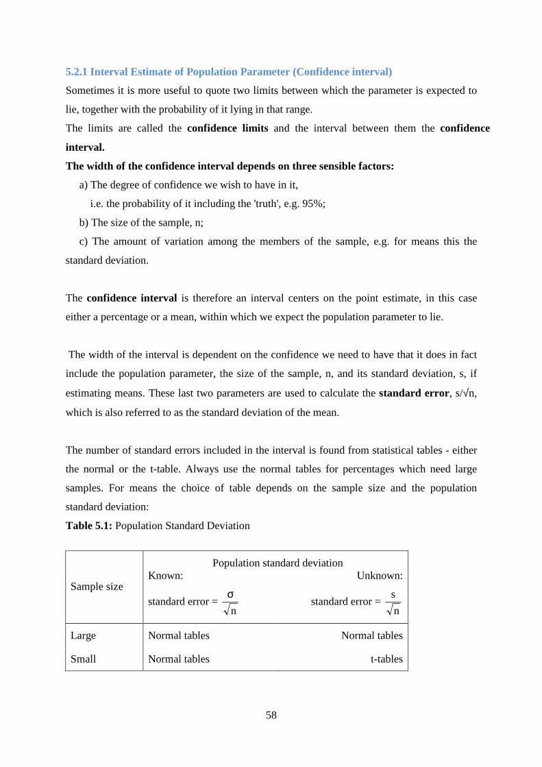
58

5.2.1 Interval Estimate of Population Parameter (Confidence interval)

Sometimes it is more useful to quote two limits between which the parameter is expected to

lie, together with the probability of it lying in that range.

The limits are called the confidence limits and the interval between them the confidence

interval.

The width of the confidence interval depends on three sensible factors:

a) The degree of confidence we wish to have in it,

i.e. the probability of it including the 'truth', e.g. 95%;

b) The size of the sample, n;

c) The amount of variation among the members of the sample, e.g. for means this the

standard deviation.

The confidence interval is therefore an interval centers on the point estimate, in this case

either a percentage or a mean, within which we expect the population parameter to lie.

The width of the interval is dependent on the confidence we need to have that it does in fact

include the population parameter, the size of the sample, n, and its standard deviation, s, if

estimating means. These last two parameters are used to calculate the standard error, s/√n,

which is also referred to as the standard deviation of the mean.

The number of standard errors included in the interval is found from statistical tables - either

the normal or the t-table. Always use the normal tables for percentages which need large

samples. For means the choice of table depends on the sample size and the population

standard deviation:

Table 5.1: Population Standard Deviation

Population standard deviation

Sample size Known:

standard error = n

σ

Unknown:

standard error = n

s

Large Normal tables Normal tables

Small Normal tables t-tables

59

5.2.2 Interpretation of Confidence intervals

How do we interpret a confidence interval? If 100 similar samples were taken and analyzed

then, for a 95% confidence interval, we are confident that 95 of the intervals calculated would

include the true population mean. In practice we tend to say that we are 95% confident that

our interval includes the true population value. Note that there is only one true value for the

population mean, it is the variation between samples which gives the range of confidence

intervals.

In Text Question

The confidence interval is therefore an interval centers on the vertical estimate. True/False

In Text Answer

False (Point)

5.2.3 Confidence Intervals for a Percentage or Proportion

The only difference between calculating the interval for percentages or for proportions is that

the former total 100 and the latter total 1. This difference is reflected in the formulae used,

otherwise the methods are identical. Percentages are probably the more commonly calculated

so in Example 2 we will estimate a population percentage.

The confidence interval for a population percentage or a proportion, π, is given by:

( )n

p100pzp

−±=π for a percentage or ( )

n

p1pzp

−±=π for a proportion

where: π is the unknown population percentage or proportion being estimated,

p is the sample percentage or proportion, i.e. the point estimate for π,

z is the appropriate value from the normal tables,

n is the sample size.

The formulae ( )

n

p100p − and

( )n

p1p − represent the standard errors of a percentage and

a proportion respectively.

The samples must be large, ( >30), so that the normal table may be used in the formula.

60

We therefore estimate the confidence limits as being at z standard errors either side of the

sample percentage or proportion.

The value of z, from the normal table, depends upon the degree of confidence, e.g. 95%,

required. We are prepared to be incorrect in our estimate 5% of the time and confidence

intervals are always symmetrical so, in the tables we look for Q to be 5%, two tails.

Example 1 If we say a distance is 5.15 metres, we are giving a point estimate. If, on the other hand, we

say that the distance is 5.15 ± 0.12 metres, i.e. the distance between 5.03 and 5.27 metres, we

are giving an interval estimate.

5.2.4 Interval Estimation

In this section, our aim is to estimate the interval to which the population parameter of

interest lies. Given the sample mean, X and variance S2, we intend to estimate the

corresponding population parameters, that is, µ and σ2.

Assume that µs and σs are the mean and standard deviation (error) of the sampling

distribution of a statistic S. Then, for the distribution to be normal, it is expected to lie in the

interval µs ± σs, µs ± 2σs, µs ± 3σs. This gives about 68.27%, 95.45% and 99.73% of the

time respectively.

Similarly, we can be confident of finding µs in the intervals S ± σs, S ± 2σs, S ± 3σs in about

68.27%, 95.45% and 99.73% of the time respectively. The respective intervals are called the

68.27%, 95.45% and 99.73% confidence intervals for estimating the population parameter, µs

(in the case of an unbiased S).

The end numbers of the interval are called the confidence limits. The percentage confidence

is called the confidence level. The numbers 1.0, 2.0, 3.0, 1.98, 2.58, etc in the confidence

limits are called the critical values (or confidence coefficients). Because of repeated use, we

are going to make use of certain areas under the standard normal curve, let us take a look at

them.

61

( 2 2 ) 0.9545T T TP T Tσ µ σ− ≤ ≤ + = and ( ) 0.6827T T TP T Tσ µ σ− ≤ ≤ + =

The statement 1 2( ) 1TP t tµ α≤ ≤ = − , say, means that we expect the interval [ ]1 2,t t to cover

Tµ , 100(1 )%α− of the time; which is to say that we are 100(1 )%α− confident that [ ]1 2,t t

covers Tµ . [ ]1 2,t t is called a confidence interval for estimating Tµ . The end points of the

interval are called confidence limits. The amount of confidence in any interval is called the

confidence coefficient.

Summary


1. Estimation

Estimation is a process by which a statistic (summary of a collection of numerical data e.g.


population from which the sample has been drawn.

2. Interval Estimate An estimate of a population parameter given by two numerical values between which the

parameter may be considered to lie with a given probability is called an interval estimate of

the parameter






end of this Module.


Define Estimation


Explain Confidence interval

62

References

John, E. F. (1974). Modern Elementary Statistics, International. London: Edition. Prentice

Hall.






Publications


63

Study Session 6: Large Sample Interval Estimation for Means

and Proportions

Introduction

A point estimate of a population parameter is a single value of a statistic. For example, the

sample mean x is a point estimate of the population mean µ. Similarly, the sample proportion

p is a point estimate of the population proportion P. Interval estimate.

The aim of this study session is to introduce you to large sample interval estimation of means

and proportions. You shall also work examples on large sample estimation of means and

proportions.



6.1 Large Sample Estimation of a Population Mean


6.1 Large Sample Interval Estimation for Mean

If the statistic S is the sample mean x , then 95% and 99% confidence level for estimation of

the population mean µ, are given by 1.96 xx σ± and 2.58 xx σ± respectively. Generally, the

confidence limits are given as xix Zσ± , where Zi is the level of confidence desired and can

be got from the table. The sample variance is then given as 2

n

σ. Thus, the confidence interval

for the population mean is then given as cx Zn

σ± .

This becomes ( , )c cX Z X Zn n

σ σ+ − and the confidence limit is without the brackets that is

64

,c cX Z X Zn n

σ σ+ − . This is where sampling is from an infinite population, or if it is with

replacement from a finite population. But if sampling is without replacement from a

population of size N, the confidence interval for the population mean is ( )1

c

N nX Z

Nn

σ −±

−

Note: If σ2 is not known provided n the sample size is sufficiently large for an infinite

population or when population is finite provided sampling is done with replacement we may

use ( )22 1

1iS X X

n= −

− ∑ in place of σ2, the approximation is still fair for the normal

distribution.

Example 1

The mean weight of a random sample of 80 yams from a farm is 3.75kg with a standard

deviation 0.85kg. Find (i) 95% (ii) (97.5%) (iii) 99% confidence interval for the population

mean of all yams on the farm.

Solution: 95% = 0.95, α = 0.05, Z1-α /2= Z0.975 = 1.96

The confidence interval is = 1.96 , 1.96x xn n

σ σ− +

The required C.I. for population mean is

i. = 1.961

Sx

n±

−

= 0.85

3.75 1.9679

x±

= (3.56, 3.94)

ii. We want 97.5% = 0.975 but α = 0.025, 2

α = 0.0125

Z1-α/2= Z0.9875 = 2.24

The required confidence interval is0.85 0.85

3.75 2.24 , 3.75 2.2479 79

x x− +

= (3.54, 3.96)

65

iii. 99% = 0.99, 0.01

,2 2

α= Z1 -α /2= Z0.995 = 2.58 The required C.I. is

= 0.85

3.75 2.5879

x±

= (3.50, 4.00)


The Central Limit Theorem says that, for large samples (samples of size n ≥ 30), when

viewed as a random variable the sample mean X−− is normally distributed with mean

µX−−=µ and standard deviation σX−−=σ/n−−√. The Empirical Rule says that we must go

about two standard deviations from the mean to capture 95% of the values of X−− generated

by sample after sample.

A more precise distance based on the normality of X−− is 1.960 standard deviations, which is

E=1.960σ/n−−√.

The key idea in the construction of the 95% confidence interval is this, as illustrated in Figure

"When Winged Dots Capture the Population Mean": because in sample after sample 95% of

the values of X−−lie in the interval [µ−E,µ+E], if we adjoin to each side of the point

estimate x−− a “wing” of length E, 95% of the intervals formed by the winged dots contain

µ.

The 95% confidence interval is thus x−−±1.960σ/n−−√. For a different level of confidence,

say 90% or 99%, the number 1.960 will change, but the idea is the same.

66

Figure 6.1: When Winged Dots Capture the Population Mean

"Computer Simulation of 40 95% Confidence Intervals for a Mean" shows the intervals

generated by a computer simulation of drawing 40 samples from a normally distributed

population and constructing the 95% confidence interval for each one. We expect that about

(0.05)(40)=2 of the intervals so constructed would fail to contain the population mean µ,

and in this simulation two of the intervals, shown in red, do.

It is standard practice to identify the level of confidence in terms of the area α in the two tails

of the distribution of X−− when the middle part specified by the level of confidence is taken

out.

This is shown in figure 6.2, drawn for the general situation, and in figure 6.2, drawn for 95%

confidence. Remember from Section 5.4.1 "Tails of the Standard Normal Distribution" in

study session 5 "Continuous Random Variables" that the z-value that a cut off a right tail of

area c is denoted zc. Thus the number 1.960 in the example is z.025, which is zα⁄2 for

α=1−0.95=0.05.

Figure 6.2: Normal Distribution For 100(1−α)% confidence the area

in each tail is α⁄2.

67

Figure 6.3: Normal Distribution For 95% confidence the area in each tail is

α⁄2=0.025.

The level of confidence can be any number between 0 and 100%, but the most common

values are probably 90% (α=0.10

), 95% (α=0.05), and 99% (α=0.01). Thus in general for a 100(1−α) % confidence interval,

E=zα⁄2(σ/n−−√), so the formula for the confidence interval is x−−±zα⁄2(σ/n−−√). While

sometimes the population standard deviation σ is known, typically it is not. If not, for n ≥ 30

it is generally safe to approximate σ by the sample standard deviation s.

Table 6.1: Table of Sample

As mentioned earlier, the number E=zα⁄2σ/n−−√ or E=zα⁄2s/n−−√ is called the margin of

error of the estimate.

68

6.2.1 Large Sample Interval Estimation of Proportion

If Tn =p, the proportion exhibiting a certain attribute in a sample of size n and the proportion

exhibiting the attribute in the population is p, the 100(1-α )% confidence interval for P is

given by 1

2

pqP Z

nα

−± , if sampling is from an infinite population or when it is from a finite

population but sampling is done with replacement. If sampling is without replacement from a

finite population of size N, the 100(1-α )% confidence interval is 1

2

( )1

pq N nP Z

n Nα−

−±−

where 1

2

Z α−

is the(1 )2

α− th quantile of the standard normal distribution

Example 1

A random of 1000 eligible voters in a country reveals that 575 of them would want the

National Anthem replaced. What is the 95% confidence limits for estimating the proportion

of eligible voters in the country who would want a new Anthem.

Solution

P= 575/1000=0.575

95% confidence limits are

12

pqP Z

nα

−± =

0.575 0.4250.575 1.96

1000

×±

that is 0.54436, 0.60564

Summary


1. Large Sample Interval Estimation for Mean


the population mean µ, are given by 1.96 xx σ± and 2.58 xx σ± respectively.

2. Large Sample Estimation of a Population Mean



µX−−=µ and standard deviation σX−−=σ/n−−√.

69






end of this Module.


Explain the Large Sample Interval Estimation for Mean


Discuss the Large Sample Estimation of a Population Mean

References

John, E. F.(1974). Modern Elementary Statistics, London. International Edition. Prentice

Hall.


York:McGraw-Hill Book Company




Publications

Shangodoyin D. K. et al (2002). Statistical Theory and Methods. Ibadan: Joytal Press.

70

Study Session 7: Large Sample Interval Estimation for Difference

of Means and Proportions

Introduction

Two-sample t-tests are among the most common statistical analyses performed to compare –

as the name implies – two samples comprised of continuous data satisfying parametric

assumptions. What are you actually doing, though, when you perform a t - test to compare

sample means?

Usually, you want to know if the samples are from the same population (i.e. are the means

statistically equal, based on your confidence level?) or from different populations (i.e. are the

means significantly different, based on your confidence level?). You perform a two-sample

t-test to help you make that decision.

The aim of this study session is to introduce you to large sample interval estimation of

difference of means and proportions. Furthermore, you shall work examples on large sample

estimation of difference of means and proportions.



7.1 Highlight on Two-Sample Test of Means

7.2 Explain When to Use Two-Sample t-Tests

7.3 Discuss on Two – Sample Test of Proportions – Large Sample

71

7.1 Two Sample Test of Means

When you perform a two-sample t- test, you are actually testing whether the difference

between the sample means is equal to zero. How does that work conceptually? Well, if two

samples were exactly the same, the difference in means would be equal to zero and the

distributions would be perfectly overlapping.

For samples with identical means,µ1–µ2= 0 The distributions for identical samples would be

perfectly overlapping. However, what happens as the samples begin to differ? Then, the

difference in means is not equal to zero, and you start to see a separation of means. As that

difference becomes greater, it becomes less and less likely that the two samples were taken

from the same population.

At a large enough difference (and also depending on the sample spread, of course), you may

decide that it is unlikely that the two samples are from the same population and you could

conclude that the samples are significantly different (or that the difference in means in

significantly different from zero).

For two-sample t-tests, the null and alternative hypotheses are as follows: H0 = Difference

between sample means is equal to zero (i.e., sample n means do not differ significantly) H1 =

Difference between sample means ≠ zero (i.e., sample means are significantly different)

Mathematically, how is the test statistic calculated (i.e., what is calculated to help you

determine whether the difference in means is sufficiently greater than zero to make you think

the samples are from different populations)?

Generally, the test statistic (t) is found as follows (with some variation based on equal sample

variances, paired versus unpaired data, etc.): != Where µ1 and µ2 are the sample means, SD 1

and SD2 are the corresponding sample standard deviations, and n1 and n2 are the

corresponding sample sizes. Calculating the test statistic (t) allows you to find the p-value, or

probability, of finding a difference that large or a more extreme difference given that the null

hypothesis is true.

72

In Text Question

When you perform a two-sample t- test, you are actually testing whether the difference

between the sample means is equal to

(a) Zero

(b) One

(c) Two

(d) Three.

In Text Answer

The answer is (a) Zero

7.2 When to Use Two-Sample t-Tests

You can use two-sample t-tests to determine whether two samples are likely or unlikely to

have been selected from the same population (i.e., to decide whether two samples differ

significantly based on the selected confidence level).Two- sample t-tests are, at times,

overused in place of other more appropriate statistical tests because they are very familiar to

many researchers.

However, be careful – there are specific types of data for which t-tests are appropriate, and

many for which they aren’t.

Two-sample t-tests are appropriate when:

• You are only comparing TWO samples (if > 2, consider ANOVA or other multi-

sample test to avoid increased likelihood of Type I error occurring)

• Samples are from normally distributed populations (see document re: tests for

normality)

• Samples are randomly selected and independent

• Sample data are at least interval or ratio level data (differences between values are

meaningful)

To perform two-sample t- tests, your samples do not need to:

• Have equal variances (Welch approximation)

• Have equal sample size

• Have a minimum sample size, so long as the assumptions hold (this is one of the

greatest things about a t-test) Paired versus Unpaired Data

73

When performing two-sample t-tests, it is important to know whether your data is paired or

unpaired.

In paired data, each data point in one sample is associated with (or related to) a single data

point in the second sample. The data sets cannot be analyzed as completely independent data

sets, because of the point-to-point associations between the sample data.

Examples of experiments with paired data are:

• Sample 1 taken at Time 0 days for 20 people (before treatment) to measure

cholesterol.

• Sample 2 taken at Time 30 days for the same 20 people (following treatment).

• A experiment with 30 sets of twins (one male, one female) to investigate sex-

dependent brain development.

Alternatively, unpaired data are data from samples where there is no relation or

association between a data point in one sample set and any data point in another

sample set.

Examples of experiments with unpaired data are:

• A comparison of blood sugar levels in diabetic patients versus non-diabetic patients

• An experiment in which 15 petri -plates of bacteria are treated with chlorine, and 15

are treated with EDTA

• Measuring zinc oxide concentrations in mussels from a shoreline in California and

from a shoreline in Oregon.

In Text Question

Two-sample t-tests are appropriate when Samples are randomly selected and independent.

True/False

In Text Answer

True

74

7.3 Two – Sample Test of Proportions – Large Sample

Confidence Intervals to Estimate the Difference between Two Population Proportions: p1−p2

Point estimate is the difference between the two sample proportions, written as:

p^1−p^2=y1n1−y2n2

The mean of its sampling distribution is p1−p2 and the standard deviation is given by:

p1^(1−p1^)n1+p2^(1−p2^)n2−−−−−−−−−−−−−−−−−−−√

When the observed number of successes and the observed number of failures are greater than

or equal to 5 for both populations, then the sampling distribution of p^1−p^2 is

approximately normal and we can use z-methods.

In the following, the formula of the confidence interval and the test statistic are given for

reference. You can use Minitab to perform the inference. It is more important to recognize

the problem and be able to use Minitab to draw a conclusion than to train yourself to use the

tedious formula. The 100(1−α) % confidence interval of p1−p2 is given by:

p^1−p^2±zα/2⋅s.e.(p^1−p^2) where

s.e.(p^1−p^2)=p1^(1−p1^)n1+p2^(1−p2^)n2−−−−−−−−−−−−−−√ when, again, the following

conditions are satisfied:

The number of successes and failures in both populations is larger than or equal to 5. We

will base this on the number of successes and failures in both samples. Why the samples? If

you recall in our discussion for the test of one proportion, this check of conditions used np0

and n(1−p0) where p0 was the assumed null hypothesis population proportion.

However, here where we are comparing two proportions, we do not know what the

population proportions are; but we are assuming that they are equal. For instance, the two

population proportions could be 0.65 or 0.30, etc. It doesn't matter as we are assuming they

are equal. As a result we do not have a fixed population value to use - thus substitute with

the sample proportions for each group.

Hypothesis Testing to Compare Two Population Proportions: p1,p2 When we want to check

whether two proportions are different or the same, the two-tailed test is appropriate. If we

want to see whether it is true that p1≠p2, that can be written as p1−p2≠0.

75

Note: To check whether it is true that that p1>p2 , that can be written as p1−p2>0. For

p1<p2, that can be written as p1−p2<0

.The test statistic is:

Z∗=p^1−p^2p∗(1−p∗)(1n1+1n2)−−−−−−−−−−−−−−−−√ where p∗=x1+x2n1+n2.

Note: In the denominator we assume that the two proportions have the same variances and

estimate that by the pooled estimate.

In other words, if the two population proportions are assumed equal, then we combine the

results from the two samples into one sample proportion: the total number of success in the

two samples divided by the total sample size of the two samples. This is what p∗ is

representing. In Minitab, you need to get into options and select "Use pooled estimate of p

for test." If you don't think that is reasonable to assume, then don't check the option.

Let p1 and p2 denote the proportions showing an attribute in populations 1 and 2. We wish to

compare the null hypothesis

0 1 2:H p p= with any one of the alternatives

,: 2111 ppH > ,: 2112 ppH < 2113 : ppH ≠

We have seen that the sample proportion p1, say if n is sufficiently large, has the normal

distribution with mean p1 and variance p1q1/n1. Similarly 2 2 2 2 2~ ( , / )p N p p q n so that

1 2

1 1 2 2

1 2

( )

p pZ

p q p q

n n

−=

+

Example 2

A sample poll of 240 registered voters’ from state A shows 60.3% favouring party A while

another poll of 200 registered voters taken at the same time from state B shows 53.5%. Using

a 0.01 size test, would you conclude that state A has more supporters for party A than state B

;:0 BA PPH = BA PPH >:1

P= (240x0.603+200x0.535)/440=0.572

0474.0=− BA PPσ

76

Z=(0.603-0.535)/0.0474=1.43

Decision Rule: Reject null hypothesis if Z>2.33. We cannot reject null hypothesis.

Summary


1. Two – Sample Test of Means

When you perform a two-sample t- test, you are actually testing whether the

difference between the sample means is equal to zero.

2. When to Use Two-Sample t-Tests

You use two-sample t-tests to determine whether two samples are likely or unlikely

to have been selected from the same population (i.e., to decide whether two samples

differ significantly based on the selected confidence level).Two- sample t-tests are, at

times, overused in place of other more appropriate statistical tests because they are

very familiar to many researchers.

3. Two – Sample Test of Proportions – Large Sample

Confidence Intervals to Estimate the Difference between Two Population Proportions: p1−p2

Point estimate is the difference between the two sample proportions, written as:

p^1−p^2=y1n1−y2n2

The mean of its sampling distribution is p1−p2 and the standard deviation is given by:

p1^(1−p1^)n1+p2^(1−p2^)n2−−−−−−−−−−−−−−−−−−−√

When the observed number of successes and the observed number of failures are greater than

or equal to 5 for both populations, then the sampling distribution of p^1−p^2 is

approximately normal and we can use z-methods.

77






end of this Module.


Briefly discuss Two – Sample Test of Means


Highlight on When to Use Two-Sample t-Tests


Discuss on Two – Sample Test of Proportions – Large Sample

References


Hall.




Publications


78

Study Session 8: Tests of Hypothesis

Introduction

A hypothesis test is a statistical test that is used to determine whether there is enough

evidence in a sample of data to infer that a certain condition is true for the entire population.

A hypothesis test examines two opposing hypotheses about a population: the null hypothesis

and the alternative hypothesis.

This study session presents tests of hypothesis. Null and alternative hypothesis will be

discussed. Test Statistic, Critical Region, Significance level and general procedure for testing

hypothesis will be discussed as well.



8.1 Highlight on the Hypothesis

8.2 Explain Hypothesis Testing (P-value approach)

8.3 Discuss Null Hypothesis

8.1 Hypothesis Testing

A statistical hypothesis is a statistical statement, which may or may not be true concerning

one or more populations. A test of hypothesis is a rule, which, on the basis of relevant

statistic, leads to a decision to accept or reject the null hypothesis.

The rejection of H0 when it is true is called a Type I error and the acceptance of H1 when it is

false is called a Type II error.

The hypothesis 20, 20θ θ≤ > are composite given that ~ ( , 25)X N θ whereas the hypothesis

20θ = is simple for it completely specifies that the distribution of X is N(20, 25)

79

8.2 Hypothesis Testing (P-value approach)

You are going to examine the P-Value Approach

P-value approach

The P-value approach involves determining "likely" or "unlikely" by determining the

probability assuming the null hypothesis were true of observing a more extreme test statistic

in the direction of the alternative hypothesis than the one observed. If the P-value is small,

say less than (or equal to) α, then it is "unlikely." And, if the P-value is large, say more than

α, then it is "likely."

If the P-value is less than (or equal to) α, then the null hypothesis is rejected in favor of the

alternative hypothesis. And, if the P-value is greater than α, then the null hypothesis is not

rejected.

Specifically, the four steps involved in using the P-value approach to conducting any

hypothesis test are:

1. Specify the null and alternative hypotheses.

2. Using the sample data and assuming the null hypothesis is true, calculate the value of

the test statistic. Again, to conduct the hypothesis test for the population mean µ, we

use the t-statistic t∗=x¯ −µs/n√ which follows a t-distribution with n - 1 degrees of

freedom.

2. Using the known distribution of the test statistic, calculate the P-value: "If the null

hypothesis is true, what is the probability that we'd observe a more extreme test

statistic in the direction of the alternative hypothesis than we did?" (Note how this

question is equivalent to the question answered in criminal trials:

"If the defendant is innocent, what is the chance that we'd observe such extreme

criminal evidence?")

3. Set the significance level, α, the probability of making a Type I error to be small —

0.01, 0.05, or 0.10. Compare the P-value to α. If the P-value is less than (or equal to)

80

α, reject the null hypothesis in favor of the alternative hypothesis. If the P-value is

greater than α, do not reject the null hypothesis.

In our example concerning the mean grade point average, suppose that our random sample of

n = 15 students majoring in mathematics yields a test statistic t* equaling 2.5. Since n = 15,

our test statistic t* has n - 1 = 14 degrees of freedom. Also, suppose we set our significance

level α at 0.05, so that we have only a 5% chance of making a Type I error.

The P-value for conducting the right-tailed test H0 : µ = 3 versus HA : µ > 3 is the probability

that we would observe a test statistic greater than t* = 2.5 if the population mean µ really

were 3. Recall that probability equals the area under the probability curve. The P-value is

therefore the area under a tn - 1 = t14 curve and to the right of the test statistic t* = 2.5. It can be

shown using statistical software that the P-value is 0.0127:

Figure 8.1: P-Value Hypothesis Test 1

The P-value, 0.0127, tells us it is "unlikely" that we would observe such an extreme test

statistic t* in the direction of HA if the null hypothesis were true. Therefore, our initial

assumption that the null hypothesis is true must be incorrect. That is, since the P-value,

0.0127, is less than α = 0.05, we reject the null hypothesis H0 : µ = 3 in favor of the

alternative hypothesis HA : µ > 3.

Note that we would not reject H0 : µ = 3 in favor of HA : µ > 3 if we lowered our willingness

to make a Type I error to α = 0.01 instead, as the P-value, 0.0127, is then greater than α =

0.01.

In our example concerning the mean grade point average, suppose that our random sample of

81

n = 15 students majoring in mathematics yields a test statistic t* instead equaling -2.5.

The P-value for conducting the left-tailed test H0 : µ = 3 versus HA : µ < 3 is the probability

that we would observe a test statistic less than t* = -2.5 if the population mean µ really were

3. The P-value is therefore the area under a tn - 1 = t14 curve and to the left of the test statistic

t* = -2.5. It can be shown using statistical software that the P-value is 0.0127:


The P-value, 0.0127, tells us it is "unlikely" that we would observe such an extreme test

statistic t* in the direction of HA if the null hypothesis were true. Therefore, our initial

assumption that the null hypothesis is true must be incorrect. That is, since the P-value,

0.0127, is less than α = 0.05, we reject the null hypothesis H0 : µ = 3 in favor of the

alternative hypothesis HA : µ < 3.

Note that we would not reject H0 : µ = 3 in favor of HA : µ < 3 if we lowered our willingness


0.01.

In our example concerning the mean grade point average, suppose again that our random

sample of n = 15 students majoring in mathematics yields a test statistic t* instead equaling -

2.5. The P-value for conducting the two-tailed test H0 : µ = 3 versus HA : µ ≠ 3 is the

probability that we would observe a test statistic less than -2.5 or greater than 2.5 if the

population mean µ really were 3.

82

That is, the two-tailed test requires taking into account the possibility that the test

statistic could fall into either tail (and hence the name "two-tailed" test). The P-value

is therefore the area under a tn - 1 = t14 curve to the left of -2.5 and to the right of the

2.5. It can be shown using statistical software that the P-value is 0.0127 + 0.0127, or

0.0254


Note that the P-value for a two-tailed test is always two times the P-value for either of the

one-tailed tests. The P-value, 0.0254, tells us it is "unlikely" that we would observe such an

extreme test statistic t* in the direction of HA if the null hypothesis were true.

Therefore, our initial assumption that the null hypothesis is true must be incorrect. That is,

since the P-value, 0.0254, is less than α = 0.05, we reject the null hypothesis H0 : µ = 3 in

favor of the alternative hypothesis HA : µ ≠ 3.

Note that we would not reject H0 : µ = 3 in favor of HA : µ ≠ 3 if we lowered our willingness


0.01.

83

Now that we have reviewed the critical value and P-value approach procedures for each of

three possible hypotheses, let's look at three new examples — one of a right-tailed test, one of

a left-tailed test, and one of a two-tailed test.

The good news is that, whenever possible, we will take advantage of the test statistics and P-

values reported in statistical software, such as Minitab, to conduct our hypothesis tests in this

course.

In Text Question

The P-value approach involves determining "likely" or "unlikely". True/False

In Text Answer

True

8.3 Null Hypothesis

A hypothesis is a speculation or theory based on insufficient evidence that lends itself to

further testing and experimentation. With further testing, a hypothesis can usually be proven

true or false. Let's look at an example. Little Susie speculates, or hypothesizes, that the

flowers she waters with club soda will grow faster than flowers she waters with plain water.

She waters each plant daily for a month (experiment) and proves her hypothesis true!

A null hypothesis is a hypothesis that says there is no statistical significance between the two

variables in the hypothesis. It is the hypothesis that the researcher is trying to disprove.

In the example, Susie's null hypothesis would be something like this: There is no statistically

significant relationship between the type of water I feed the flowers and growth of the

flowers. A researcher is challenged by the null hypothesis and usually wants to disprove it, to

demonstrate that there is a statistically-significant relationship between the two variables in

the hypothesis.

8.3.1 Alternative Hypothesis

An alternative hypothesis simply is the inverse, or opposite, of the null hypothesis. So, if we

continue with the above example, the alternative hypothesis would be that there IS indeed a

statistically-significant relationship between what type of water the flower plant is fed and

84

growth. More specifically, here would be the null and alternative hypotheses for Susie's

study:

Null: If one plant is fed club soda for one month and another plant is fed plain water, there

will be no difference in growth between the two plants.

Alternative: If one plant is fed club soda for one month and another plant is fed plain water,

the plant that is fed club soda will grow better than the plant that is fed plain water.

The hypothesis, H0 is called the Null hypothesis while H1 is called the Alternative

hypothesis. The former (H0) is a statement or an assumption, which we want to test or which

is accepted until the evidence proves otherwise, while the latter (H1) is a statement, which

states what we suppose will happen if the null hypothesis is not correct. Thus, H1 is usually

stated as:

H1 : θ ≠ θ1 or

θ < θ0 or

θ > θ0

We partitioned the sample space into two regions c and c* such that if the sample values fall

in c, we reject H0, but if it falls in c*, we do otherwise (accept H0). The region c is called the

critical region of the rest, and it is defined as the region that corresponds to the rejection of

the null hypothesis.

We can make a mistake of accepting H1, when H0 is true or accepting H0 when H1 is true;

such mistakes are called Type I and II errors respectively.

Table 8.1: Type I and II

Decision True False

Reject H0 Type I error Correct decision

Accept H0 Correct decision Type II error

8.3.2 Level of Significance (α)

In testing a given hypothesis, the maximum probability with which we would be willing to

risk a Type I error is called the level of significance of the test. The value α needs to be

specified before any sample is drawn so that results obtained will not influence our choice.

85

8.3.3 Test Statistic

This is the statistic formula whose value has to be computed from the available sample data

and, thus, determines the acceptance or rejection of that particular known hypothesis H0

under investigation. The text statistic may require Normal, t, X2 or F approach, as the case

may be.

8.3.4 General Procedures for Testing a Statistical Hypothesis

The following steps are summarized as procedures for test of hypothesis:

1. Formulate the Null and Alternate hypothesis.

2. Determine the appropriate test statistic, and compute its value.

3. Choose α, the level of significance.

4. Determine the critical region.

5. Make a statistical decision and

6. Conclude i.e. interpret your result.

Summary


1. Hypothesis Testing

A statistical hypothesis is a statistical statement, which may or may not be true

concerning one or more populations. A test of hypothesis is a rule, which, on the basis of

relevant statistic, leads to a decision to accept or reject the null hypothesis.

2. Hypothesis Testing (P-value approach) You are going to examine the P-Value Approach

The P-value approach involves determining "likely" or "unlikely" by determining the

probability assuming the null hypothesis were true of observing a more extreme test

statistic in the direction of the alternative hypothesis than the one observed.

3. Null Hypothesis

A hypothesis is a speculation or theory based on insufficient evidence that lends itself

to further testing and experimentation. With further testing, a hypothesis can usually

be proven true or false. Let's look at an example.

Little Susie speculates, or hypothesizes, that the flowers she waters with club soda

will grow faster than flowers she waters with plain water. She waters each plant daily

for a month (experiment) and proves her hypothesis true!

86






end of this Module.


Define Hypothesis Testing


Explain Hypothesis Testing (P-value approach)


Discuss Null Hypothesis

References

John, E. F. (1974). Modern Elementary Statistics, International Edition. London: Prentice

Hall. Murray, R. S. (1972)Schaum’s Outline Series. Theory and Problems of

Statistics. New York: McGraw-Hill Book Company


Publications

Shangodoyin D. K. et al (2002). Statistical Theory and Methods. Ibadan: Joytal: Press.

87

Study Session 9: One Sample Test of Mean and Proportion –

Large Sample

Introduction

In estimation your focused will be on explicitly on techniques for one and two samples and

talk on estimation for a specific parameter (e.g., the mean or proportion of a population), for

differences (e.g., difference in means, the risk difference) and ratios (e.g., the relative risk and

odds ratio). Here we will focus on procedures for one and two samples when the outcome is

either continuous (and we focus on means) or dichotomous (and we focus on proportions).

The aim of this study session is to introduce you to one test of mean and proportion for large

sample. You shall also work examples on large sample test of mean and proportion.



9.1 One and two sided tests of significance

9.2 One – Sample Test of Mean – Large Sample

9.1 One and two sided tests of significance

When we use a test of significance to compare two groups we usually start with the null

hypothesis that there is no difference between the populations from which the data come. If

this hypothesis is not true the alternative hypothesis must be true - that there is a difference.

Since the null hypothesis specifies no direction for the difference nor does the alternative

hypothesis, and so we have a two sided test. In a one sided test the alternative hypothesis

does specify a direction - for example, that an active treatment is better than a placebo.

88

This is sometimes justified by saying that we are not interested in the possibility that the

active treatment is worse than no treatment. This possibility is still part of the test; it is part of

the null hypothesis, which now states that the difference in the population is zero or in favour

of the placebo.

A one sided test is sometimes appropriate.

Box 9.1: Luthra et al Investigated:

The effects of laparoscopy and hydrotubation on the fertility of women presenting at an

infertility clinic.1 After some months laparoscopy was carried out on those who had still not

conceived. These women were then observed for several further months and some of these

women also conceived.

The conception rate in the period before laparoscopy was compared with that afterwards. The

less fertile a woman is the longer it is likely to take her to conceive. Hence, the women who

had the laparoscopy should have a lower conception rate (by an unknown amount) than the

larger group who entered the study, because the more fertile women had conceived before

their turn for laparoscopy came.

To see whether laparoscopy increased fertility, Luthra et al tested the null hypothesis that the

conception rate after laparoscopy was less than or equal to that before. The alternative

hypothesis was that the conception rate after laparoscopy was higher than that before. A two

sided test was inappropriate because if the laparoscopy had no effect on fertility the

conception rate after laparoscopy was expected to be lower.

One sided tests are not often used, and sometimes they are not justified. Consider the

following example. Twenty five patients with breast cancer were given radiotherapy

treatment of 50 Gy in fractions of 2 Gy over 5 weeks. 2 Lung function was measured

initially, at one week, at three months, and at one year. The aim of the study was to see

whether lung function was lowered following radiotherapy.

In Text Question

One sided tests are not often used, and sometimes they are not justified. True/False

89

In Text Answer

True Some of the results are shown in the table, the forced vital capacity being compared between

the initial and each subsequent visit using one sided tests. The direction of the one sided tests

was not specified, but it may appear reasonable to test the alternative hypothesis that forced

vital capacity decreases after radiotherapy, as there is no reason to suppose that damage to the

lungs would increase it.

The null hypothesis is that forced vital capacity does not change or increases. If the forced

vital capacity increases, this is consistent with the null hypothesis, and the more it increases

the more consistent the data are with the null hypothesis. Because the differences are not all

in the same direction, at least one P value should be greater than 0.5.

What has been done here is to test the null hypothesis that forced vital capacity does not

change or decreases from visit 1 to visit 2 (nine week), and to test the null hypothesis that it

does not change or increases from visit 1 to visit 3 (three months) or visit 4 (one year). These

authors seem to have carried out one sided tests in both directions for each visit and then

taken the smaller probability.

If there is no difference in the population the probability of getting a significant difference by

this approach is 10%, not 5% as it should be. The chance of a spurious significant difference

is doubled. Two sided tests should be used, which would give probabilities of 0.26, 0.064,

and 0.38, and no significant differences.

In general a one sided test is appropriate when a large difference in one direction would lead

to the same action as no difference at all. Expectation of a difference in a particular direction

is not adequate justification. In medicine, things do not always work out as expected, and

researchers may be surprised by their results.

For example 1:

Galloe et al found that oral magnesium significantly increased the risk of cardiac events,

rather than decreasing it as they had hoped.3 If a new treatment kills a lot of patients we

should not simply abandon it; we should ask why this happened.

90

Two sided tests should be used unless there is a very good reason for doing otherwise. If one

sided tests are to be used the direction of the test must be specified in advance. One sided

tests should never be used simply as a device to make a conventionally non-significant

difference significant.

Example 2

Let us consider a test of whether a coin is symmetric or not and consider the particular

hypotheses.

1. 01 11

1 1: , :

2 2H p H p= < - One tail test lower tail

2. 02 12

1 1: , :

2 2H p H p= > - One tail test Upper tail

3. 03 13

1 1: , : .

2 2H p H p= ≠ Two tail test

where p is the probability that the coin shows a head.With the coin in the dock accused of

being biased, we call for evidence, which is the number of heads in 10 heads of the coin.In

the first case, one would be inclined to reject H0 if X is equal to, say, 0, 1, or 2 and to accept

H0 for other values of X.

That is only values of X which are extremely less than 5 will lead to the rejection of H0.In the

second case, one would be inclined to reject H0 if X takes, say, any of the values 10, 9, 8, i.e.

only values of X, which are extremely larger than 5 will lead to the rejection of H0.In the

third case, values of X, which are either extremely larger than or extremely less than 5 seem

to qualify for the critical region.

9.2 One – Sample Test of Mean – Large Sample

A hypothesis about a population mean µ may be tested by obtaining the mean of a random

sample of size n from the population. Suppose a random sample of size nA from population A

yields a mean AX ; we know that provided nA is large and sampling is done from a finite

91

population and it is done with replacement then 2~ ( , / )A A A AX N nµ σ and the test statistic is

2

A A

A

A

XZ

n

µ

σ

−= which has the standard normal distribution; µ and σ being population mean

and standard deviation respectively. When the population variance 2σ is not known but n is

sufficiently large, we may use 2 2

1

1ˆ ( )

1

n

ii

s X Xn =

= −− ∑ in its place. The approximation is still

good.

Example 1

The mean weight of 64 men is 63kg. The mean weight for the population is 60kg, with a

standard deviation of 12kg. Is the mean weight of the sample greater than the population

mean weight at the 5% level?

Solution

Set up the hypothesis

Ho : Mean Weight = 60kg

H1 : Mean Weight ≠ 60kg

( ) 12 12Se 1.5

864x = = = kilos

. ( )

xZ

S E x

µ−=

63 60 3

1.5 1.5

−= = = 2.0

Comparing the calculated Z statistic at the 5% level tabulated Z value = 1.96

Decision: Since the calculated Z value of 2.0 lie outside -1.96 and +1.96 table value of Z at

5% level of significance, we reject the null hypothesis (H0) and conclude that the mean

weight of the sample is not 60kg. The result is said to be significant at the 5% level.

9.2.1 One Sample Test- Proportion- Large Sample

Example 2

In a recent poll 0.65 of the 91 registered voters polled favoured party A, whereas the

proportion that favoured the party at the last general election before the poll was 0.575.

92

Would this be a justification for claiming an improved popularity for party A at the 0.05 level

of significance?

Solution

575.0: 00 == pPH

575.0:1 >PH

45.1

91

425.0575.0(

)575.065.0( =×

−=

The critical level for a test of size 0.05 is for an upper tail, 1.645. Hence we cannot reject 0H

Summary


1. One and two sided tests of significance

When we use a test of significance to compare two groups we usually start with the null

hypothesis that there is no difference between the populations from which the data come. If

this hypothesis is not true the alternative hypothesis must be true - that there is a difference.

2. One – Sample Test of Mean – Large Sample

A hypothesis about a population mean µ may be tested by obtaining the mean of a random

sample of size n from the population. Suppose a random sample of size nA from population A

yields a mean AX ; we know that provided nA is large and sampling is done from a finite

population and it is done with replacement then 2~ ( , / )A A A AX N nµ σ and the test statistic is

2

A A

A

A

XZ

n

µ

σ

−= which has the standard normal distribution; µ and σ being population mean

and standard deviation respectively. When the population variance 2σ is not known but n is

sufficiently large, we may use 2 2

1

1ˆ ( )

1

n

ii

s X Xn =

= −− ∑ in its place. The approximation is still

good.

93






end of this Module.


Briefly explain One and two sided tests of significance


Discuss One Sample Test of Mean – Large Sample

References

John, E. F.(1974). Modern Elementary Statistics, International Edition. London: Prentice

Hall.




Publications


Lund MB, Myhre KI, Melsom H, Johansen B The effect on pulmonary function of tangential

field technique in radiotherapy for carcinoma of the breast. Br J Radiol 1991;64:520–3.

Luthra P, Bland JM, Stanton SL Incidence of pregnancy after laparoscopy and hydrotubation.

BMJ 1982;284:1013.

Galloe AM, Rasmussen HS, Jorgensen LN, Aurup P, Balslov S, Cintin C, Graudal N,

McNair P

Influence of oral magnesium supplementation on cardiac events among survivors of an acute

myocardial infarction. BMJ 1993;307:585–7.

94

Study Session 10: Two Sample Test of Means and Proportions –

Large Sample

Introduction

The process of hypothesis testing involves setting up two competing hypotheses, the null

hypothesis and the alternate hypothesis. One selects a random sample (or multiple samples

when there are more comparison groups), computes summary statistics and then assesses the

likelihood that the sample data support the research or alternative hypothesis.

Similar to estimation, the process of hypothesis testing is based on probability theory and the

Central Limit Theorem.



10.1 Explain Two-Sample t-Test for Equal Means 10.2 Discuss Test Statistics for Testing

10.1 Two-Sample t-Test for Equal Means

Purpose Test if two population means are equal:

The two-sample t-test is used to determine if two population means are equal. A

common application is to test if a new process or treatment is superior to a

current process or treatment.

There are several variations on this test:

1. The data may either be paired or not paired. By paired, we mean that

there is a one-to-one correspondence between the values in the two

samples. That is, if X1, X2, ..., Xn and Y1, Y2, ... , Yn are the two samples,

then Xi corresponds to Yi. For paired samples, the difference Xi - Yi is

usually calculated.

For unpaired samples, the sample sizes for the two samples may or may

95

not be equal. The formulas for paired data are somewhat simpler than

the formulas for unpaired data.

2. The variances of the two samples may be assumed to be equal or

unequal. Equal variances yields somewhat simpler formulas, although

with computers this is no longer a significant issue.

3. In some applications, you may want to adopt a new process or treatment

only if it exceeds the current treatment by some threshold. In this case,

we can state the null hypothesis in the form that the difference between

the two populations means is equal to some constant µ1−µ2=d0 where

the constant is the desired threshold.

Definition The two-sample t-test for unpaired data is defined as:

H0: µ1=µ2

Ha: µ1≠µ2

Test

Statistic:

T=Y1¯ −Y2 s̄21/N1+s22/N2√ where N1 and N2 are the sample

sizes, Y1¯ and Y2¯ are the sample means, and s21 and s22 are the

sample variances. If equal variances are assumed, then the

formula reduces to: T=Y1¯ −Y2 s̄p1/N1+1/N2√ where

s2p=(N1−1)s21+(N2−1)s22N1+N2−2

Significance

Level:

α.

Critical

Region:

Reject the null hypothesis that the two means are equal if

|T| > t1-α/2,ν where t1-α/2,ν is the critical value of the t

distribution with ν degrees of freedom where

υ=(s21/N1+s22/N2)2(s21/N1)2/(N1−1)+(s22/N2)2/(N2−1)

If equal variances are assumed, then ν = N1 + N2 - 2

Two Sample t- Test Example

The following two-sample t-test was generated for the auto83b.dat data set. The

data set contains miles per gallon for U.S. cars (sample 1) and for Japanese cars

(sample 2); the summary statistics for each sample are shown below.

96

SAMPLE 1: number of observations = 249 MEAN = 20.14458

Standard Deviation = 6.41470 Standard Error Of The Mean = 0.40652

SAMPLE 2:

Number Of Observations = 79

Mean = 30.48101

Standard Deviation = 6.10771

Standard Error Of The Mean = 0.68717 We are testing the hypothesis that the

population means are equal for the two samples. We assume that the variances

for the two samples are equal.

H0: µ1 = µ2

Ha: µ1 ≠ µ2 Test statistic: T = -12.62059 Pooled standard deviation: sp =

6.34260

Degrees of freedom: ν = 326

Significance level: α = 0.05 Critical value (upper tail): t1-α/2,ν = 1.9673

Critical region: Reject H0 if |T| > 1.9673

The absolute value of the test statistic for our example, 12.62059, is greater than

the critical value of 1.9673, so we reject the null hypothesis and conclude that

the two population means are different at the 0.05 significance level.

In general, there are three possible alternative hypotheses and rejection regions

for the one-sample t-test:

Alternative Hypothesis Rejection Region

Ha: µ1 ≠ µ2 |T| > t1-α/2,ν

Ha: µ1 > µ2 T > t1-α,ν

Ha: µ1 < µ2 T < tα,ν

Figure 10.1: Hypotheses and rejection regions for the one-sample t-test:

For our two-tailed t-test, the critical value is t1-α/2,ν = 1.9673, where α = 0.05 and

ν = 326. If we were to perform an upper, one-tailed test, the critical value would

97

be t1-α,ν = 1.6495. The rejection regions for three possible alternative hypotheses

using our example data are shown below.

If a random sample of size nx taken from an X-population yields mean X and an independent

one of size nY from a Y-population yields mean Y ,we know that the sampling distribution of

the difference YX − is normal with mean X Y X Yµ µ µ− = − the difference of the population

means and variance 2 2

2 2 2 X YX Y X Y

X Yn nσ σσ σ σ− = + = + where 2

Yσ is the variance of the Y-

population. i.e. 2 2

~ , .X YX Y

X Y

X Y Nn n

σ σµ µ− − +

( )

2 2~ (0,1)X Y

X Y

X Y

X YZ N

n n

µ µ

σ σ

− − −=

+

For testing the null hypothesis µX – µY = 0 or µX = µY against the alternative H1: µX ≠ µY, say,

the decision rule, is, for an α-size two-tail test:

Reject H0 if Z lies outside 2 21

( , )z zα α− :

Otherwise, do not reject it.

Observe that 2 2

( )

X Y

X Y

X Yz

n nσ σ

−=

+

when H0 holds, and it is assumed that 2

Xσ and 2

Yσ are

known.

When 2

Xσ and 2

Yσ are not known, provided nX and nY are sufficiently large, they may be

estimated by

∑=

−=Xn

iXX XX

ns

1

22 )(1

ˆ,

∑=

−=Yn

iYY XX

ns

1

22 )(1

ˆ

Example 1 The mean weight of 50 pigs raised on diet A is 68.2 k9, while that of 60 pigs raised on diet B

is 67.0 kg. Test the hypothesis that Diet A is superior to diet B if is known that the population

variance of the weights of pigs raised on A is 12.25 kg2 while that of pigs raised on B is 15.21

kg2.

Solution

Let Aµ and Bµ denote the population means of weights of pigs raised on A and B

respectively. The null hypothesis, then is

BAH µµ =:0 while the alternative is

98

BAH µµ >:1 which calls for an upper-tail test.

4985.0

60

21.15

50

25.12 =+=− BA XXσ

7.1

706.0

)0.672.68( =−=Z

Decision Rule: Reject 0H if 1.645Z ≥ for a 0.05 level of significance test.

We reject 0H on the basis of the evidence provided by the sample.

10.1.1 Tests with Two Independent Samples

There are many applications where it is of interest to compare two independent groups with

respect to their mean scores on a continuous outcome. Here we compare means between

groups, but rather than generating an estimate of the difference, we will test whether the

observed difference (increase, decrease or difference) is statistically significant or not.

Remember, that hypothesis testing gives an assessment of statistical significance, whereas

estimation gives an estimate of effect and both are important.

Here you discuss the comparison of means when the two comparison groups are independent

or physically separate. The two groups might be determined by a particular attribute (e.g.,

sex, diagnosis of cardiovascular disease) or might be set up by the investigator (e.g.,

participants assigned to receive an experimental treatment or placebo).

The first step in the analysis involves computing descriptive statistics on each of the two

samples. Specifically, we compute the sample size, mean and standard deviation in each

sample and we denote these summary statistics as follows:

for sample 1:

� n1

�

� s1

for sample 2:

� n2

99

�

� s2

The designation of sample 1 and sample 2 is arbitrary. In a clinical trial setting the

convention is to call the treatment group 1 and the control group 2. However, when

comparing men and women, for example, either group can be 1 or 2.

In the two independent samples application with a continuous outcome, the parameter of

interest in the test of hypothesis is the difference in population means, µ1-µ2. The null

hypothesis is always that there is no difference between groups with respect to means, i.e.,

The null hypothesis can also be written as follows: H0: µ1 = µ2. In the research hypothesis, an

investigator can hypothesize that the first mean is larger than the second (H1: µ1 > µ2 ), that

the first mean is smaller than the second (H1: µ1 < µ2 ), or that the means are different (H1: µ1

≠ µ2 ). The three different alternatives represent upper-, lower-, and two-tailed tests,

respectively. The following test statistics are used to test these hypotheses.

In Text Question

The designation of sample 1 and sample 2 is arbitrary. In a clinical trial setting the

convention is to call the treatment group 1 and the control group 2.True/False

In Text Answer

True

10.2 Test Statistics for Testing

The following are test of statistics of two sample mean of proportions:

H0: µ1 = µ2

� if n1 > 30 and n2 > 30

o

� if n1 < 30 or n2 < 30

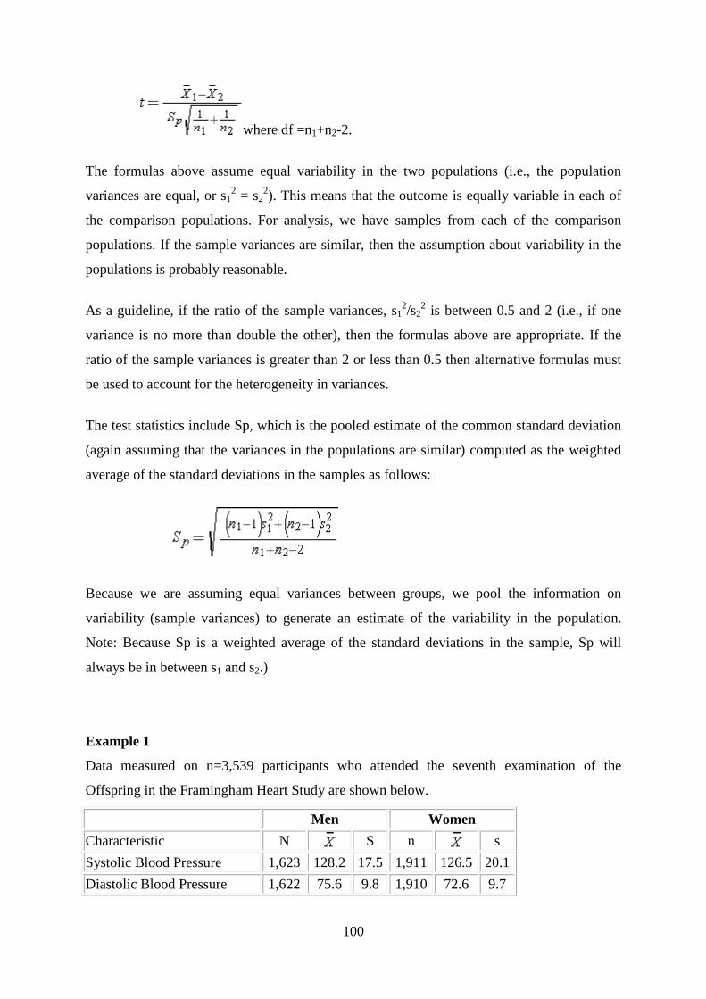
100

where df =n1+n2-2.

The formulas above assume equal variability in the two populations (i.e., the population

variances are equal, or s12 = s2

2). This means that the outcome is equally variable in each of

the comparison populations. For analysis, we have samples from each of the comparison

populations. If the sample variances are similar, then the assumption about variability in the

populations is probably reasonable.

As a guideline, if the ratio of the sample variances, s12/s2

2 is between 0.5 and 2 (i.e., if one

variance is no more than double the other), then the formulas above are appropriate. If the

ratio of the sample variances is greater than 2 or less than 0.5 then alternative formulas must

be used to account for the heterogeneity in variances.

The test statistics include Sp, which is the pooled estimate of the common standard deviation

(again assuming that the variances in the populations are similar) computed as the weighted

average of the standard deviations in the samples as follows:

Because we are assuming equal variances between groups, we pool the information on

variability (sample variances) to generate an estimate of the variability in the population.

Note: Because Sp is a weighted average of the standard deviations in the sample, Sp will

always be in between s1 and s2.)

Example 1

Data measured on n=3,539 participants who attended the seventh examination of the

Offspring in the Framingham Heart Study are shown below.

Men Women

Characteristic N

S n

s

Systolic Blood Pressure 1,623 128.2 17.5 1,911 126.5 20.1

Diastolic Blood Pressure 1,622 75.6 9.8 1,910 72.6 9.7

101

Total Serum Cholesterol 1,544 192.4 35.2 1,766 207.1 36.7

Weight 1,612 194.0 33.8 1,894 157.7 34.6

Height 1,545 68.9 2.7 1,781 63.4 2.5

Body Mass Index 1,545 28.8 4.6 1,781 27.6 5.9

Suppose we now wish to assess whether there is a statistically significant difference in mean

systolic blood pressures between men and women using a 5% level of significance.

• Step 1. Set up hypotheses and determine level of significance

H0: µ1 = µ2

H1: µ1 ≠ µ2 α=0.05

• Step 2. Select the appropriate test statistic.

Because both samples are large (> 30), we can use the Z test statistic as opposed to t. Note

that statistical computing packages use t throughout. Before implementing the formula, we

first check whether the assumption of equality of population variances is reasonable.

The guideline suggests investigating the ratio of the sample variances, s12/s2

2. Suppose we

call the men group 1 and the women group 2. Again, this is arbitrary; it only needs to be

noted when interpreting the results. The ratio of the sample variances is 17.52/20.12 = 0.76,

which falls between 0.5 and 2 suggesting that the assumption of equality of population

variances is reasonable. The appropriate test statistic is

.

• Step 3. Set up decision rule.

This is a two-tailed test, using a Z statistic and a 5% level of significance. Reject H0 if Z < -

1.960 or is Z > 1.960.

• Step 4. Compute the test statistic.

102

We now substitute the sample data into the formula for the test statistic identified in Step 2.

Before substituting, we will first compute Sp, the pooled estimate of the common standard

deviation.

Notice that the pooled estimate of the common standard deviation, Sp, falls in between the

standard deviations in the comparison groups (i.e., 17.5 and 20.1). Sp is slightly closer in

value to the standard deviation in the women (20.1) as there were slightly more women in the

sample. Recall, Sp is a weight average of the standard deviations in the comparison groups,

weighted by the respective sample sizes.

Now the test statistic:

• Step 5. Conclusion.

We reject H0 because 2.66 > 1.960. We have statistically significant evidence at α=0.05 to

show that there is a difference in mean systolic blood pressures between men and women.

The p-value is p < 0.010.

Here again we find that there is a statistically significant difference in mean systolic blood

pressures between men and women at p < 0.010. Notice that there is a very small difference

in the sample means (128.2-126.5 = 1.7 units), but this difference is beyond what would be

expected by chance. Is this a clinically meaningful difference? The large sample size in this

example is driving the statistical significance.

A 95% confidence interval for the difference in mean systolic blood pressures is: 1.7 + 1.26

or (0.44, 2.96). The confidence interval provides an assessment of the magnitude of the

103

difference between means whereas the test of hypothesis and p-value provide an assessment

of the statistical significance of the difference.

Above we performed a study to evaluate a new drug designed to lower total cholesterol. The

study involved one sample of patients, each patient took the new drug for 6 weeks and had

their cholesterol measured. As a means of evaluating the efficacy of the new drug, the mean

total cholesterol following 6 weeks of treatment was compared to the NCHS-reported mean

total cholesterol level in 2002 for all adults of 203.

At the end of the example, we discussed the appropriateness of the fixed comparator as well

as an alternative study design to evaluate the effect of the new drug involving two treatment

groups, where one group receives the new drug and the other does not. Here, we revisit the

example with a concurrent or parallel control group, which is very typical in randomized

controlled trials or clinical trials.

Example 2

A new drug is proposed to lower total cholesterol. A randomized controlled trial is designed

to evaluate the efficacy of the medication in lowering cholesterol. Thirty participants are

enrolled in the trial and are randomly assigned to receive either the new drug or a placebo.

The participants do not know which treatment they are assigned. Each participant is asked to

take the assigned treatment for 6 weeks. At the end of 6 weeks, each patient's total cholesterol

level is measured and the sample statistics are as follows.

Table 10.1 : Treatment Table

Treatment Sample

Size

Mean Standard

Deviation

New Drug 15 195.9 28.7

Placebo 15 217.4 30.3

Is there statistical evidence of a reduction in mean total cholesterol in patients taking the new

drug for 6 weeks as compared to participants taking placebo? We will run the test using the

five-step approach.

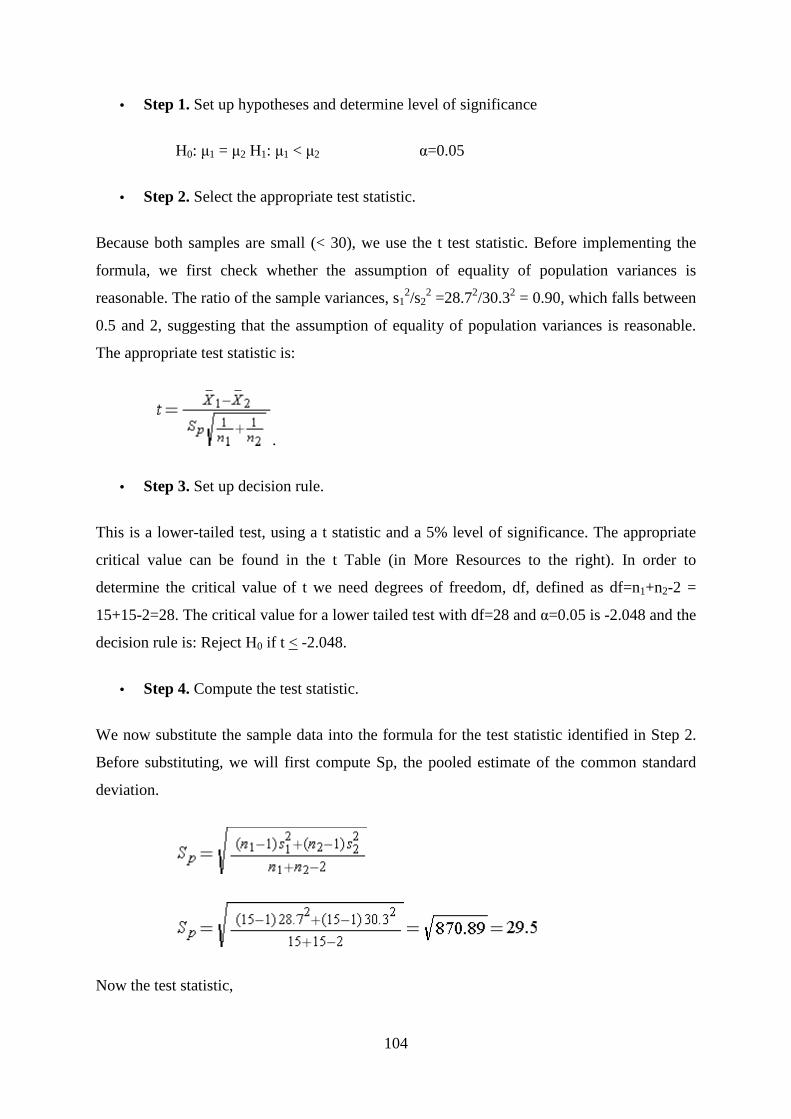
104

• Step 1. Set up hypotheses and determine level of significance

H0: µ1 = µ2 H1: µ1 < µ2 α=0.05

• Step 2. Select the appropriate test statistic.

Because both samples are small (< 30), we use the t test statistic. Before implementing the

formula, we first check whether the assumption of equality of population variances is

reasonable. The ratio of the sample variances, s12/s2

2 =28.72/30.32 = 0.90, which falls between

0.5 and 2, suggesting that the assumption of equality of population variances is reasonable.

The appropriate test statistic is:

.

• Step 3. Set up decision rule.

This is a lower-tailed test, using a t statistic and a 5% level of significance. The appropriate

critical value can be found in the t Table (in More Resources to the right). In order to

determine the critical value of t we need degrees of freedom, df, defined as df=n1+n2-2 =

15+15-2=28. The critical value for a lower tailed test with df=28 and α=0.05 is -2.048 and the

decision rule is: Reject H0 if t < -2.048.

• Step 4. Compute the test statistic.

We now substitute the sample data into the formula for the test statistic identified in Step 2.

Before substituting, we will first compute Sp, the pooled estimate of the common standard

deviation.

Now the test statistic,

105

• Step 5. Conclusion.

We reject H0 because -2.92 < -2.048. We have statistically significant evidence at α=0.05 to

show that the mean total cholesterol level is lower in patients taking the new drug for 6 weeks

as compared to patients taking placebo, p < 0.005.

The clinical trial in this example finds a statistically significant reduction in total cholesterol,

whereas in the previous example where we had a historical control (as opposed to a parallel

control group) we did not demonstrate efficacy of the new drug.

Notice that the mean total cholesterol level in patients taking placebo is 217.4 which is very

different from the mean cholesterol reported among all Americans in 2002 of 203 and used as

the comparator in the prior example. The historical control value may not have been the most

appropriate comparator as cholesterol levels have been increasing over time. In the next

section, we present another design that can be used to assess the efficacy of the new drug.

10.2.1 Two – Sample Test of Proportions – Large Sample

Let p1 and p2 denote the proportions showing an attribute in populations 1 and 2. We wish to

compare the null hypothesis

0 1 2:H p p= with any one of the alternatives

,: 2111 ppH > ,: 2112 ppH < 2113 : ppH ≠

We have seen that the sample proportion p1, say if n is sufficiently large, has the normal

distribution with mean p1 and variance p1q1/n1. Similarly 2 2 2 2 2~ ( , / )p N p p q n so that

1 2

1 1 2 2

1 2

( )

p pZ

p q p q

n n

−=

+

Example 1

A sample poll of 240 registered voters’ from state A shows 60.3% favouring party A while

106

another poll of 200 registered voters taken at the same time from state B shows 53.5%. Using

a 0.01 size test, would you conclude that state A has more supporters for party A than state B

;:0 BA PPH = BA PPH >:1

P= (240x0.603+200x0.535)/440=0.572

0474.0=− BA PPσ

Z=(0.603-0.535)/0.0474=1.43

Decision Rule: Reject null hypothesis if Z>2.33. We cannot reject null hypothesis.

Summary


(1) Two-Sample t-Test for Equal Means

The two-sample t-test is used to determine if two population means are equal. A common

application is to test if a new process or treatment is superior to a current process or

treatment.

There are several variations on this test:

1. The data may either be paired or not paired. By paired, we mean that there is a one-to-

one correspondence between the values in the two samples. That is, if X1, X2, ..., Xn

and Y1, Y2, ... , Yn are the two samples, then Xi corresponds to Yi. For paired samples,

the difference Xi - Yi is usually calculated.

For unpaired samples, the sample sizes for the two samples may or may not be equal.

The formulas for paired data are somewhat simpler than the formulas for unpaired

data.

2. The variances of the two samples may be assumed to be equal or unequal. Equal

variance yields somewhat simpler formulas, although with computers this is no longer

a significant issue.

107

3. In some applications, you may want to adopt a new process or treatment only if it

exceeds the current treatment by some threshold. In this case, we can state the null

hypothesis in the form that the difference between the two populations means is equal

to some constant µ1−µ2=d0 where the constant is the desired threshold.

(2) Test Statistics for Testing The following are test of statistics of two sample mean of proportions:

H0: µ1 = µ2

� if n1 > 30 and n2 > 30

o

� if n1 < 30 or n2 < 30

where df =n1+n2-2.

The formulas above assume equal variability in the two populations (i.e., the population

variances are equal, or s12 = s2

2). This means that the outcome is equally variable in each of

the comparison populations. For analysis, we have samples from each of the comparison

populations. If the sample variances are similar, then the assumption about variability in the

populations is probably reasonable.






end of this Module.

108


Lst Two-Sample t-Test for Equal Means


Explain Test Statistics for Testing

References


Hall.




Publications


109

Study Session 11: Regression Analysis

Introduction

Regression analysis is a statistical tool for the investigation of relationships between

variables. Usually, the investigator seeks to ascertain the causal effect of one variable upon

another the effect of a price increase upon demand, for example, or the effect of changes in

the money supply upon the inflation rate.

To explore such issues, the investigator assembles data on the underlying variables of interest

and employs regression to estimate the quantitative effect of the causal variables upon the

variable that they influence. The investigator also typically assesses the “statistical

significant” of the estimated relationships, that is, the degree of confidence that the true

relationship is close to the estimated relationship.

In this study session, you shall consider situations where two variables are observed on each

unit such data are, for instance, age, intelligence quotient data form, a bivariate data etc.

Scatter diagram will be discussed as well as least square line. We will fit least square line to

using a bivariate data.



11.1 Explain Scatter Diagram

11.2 Discuss Least Square

11.1 Scatter Diagram

Scatter graph method is a graphical technique of separating fixed and variable components of

mixed cost by plotting activity level along x-axis and corresponding total cost (mixed cost)

along y-axis. A regression line is then drawn on the graph by visual inspection.

110

The scatter diagram is known by many names, such as scatter plot, scatter graph, and

correlation chart. This diagram is drawn with two variables, usually the first variable is

independent and the second variable is dependent on the first variable.

Figure 11.1: Scatter Diagram

The scatter diagram is used to find the correlation between these two variables. This diagram

shows you how closely the two variables are related. After determining the correlation

between the variables, you can easily predict the behavior of the other variable. This chart is

very useful when one variable is easy to measure and the other is not.

For example, let’s say that you are analyzing the pattern of accidents on a highway. You

select the two variables motor speed and number of accidents, and draw the diagram.

Once the diagram is completed, you notice that as the speed of vehicle increases, the number

of accidents also goes up. This shows that there is a relation between the speed of vehicles

and accidents happening on the highway.

11.1.1 Type of Scatter Diagram

The scatter diagram can be categorized into several types of classifications; however, here I

will discuss two types of classifications that will cover most types of scatter diagrams. The

first classification is based on the type of correlation, and the second classification is based on

the slope of trend.

I am giving you two types of classifications because it will show you the same chart with two

different perspectives which will build a solid understanding for you regarding the scatter

diagram.

According to the type of c

categories:

Figure 11.2

The scatter diagram is “A correlation chart that uses a regression line to explain or to predict

how the change in an independent variable will

Scatter diagram helps you see the changes in the dependent variable if you make any change

to the independent variable. Since this diagram shows you the correlation between the

variables, it is also known as a correlation cha

Usually independent variable is plotted along the horizontal axis (x

variable is plotted on the vertical axis (y

control parameter because it influences the behavior of the depen

It is not necessary for one parameter to be a controlling parameter. You can draw the scatter

diagram with both variables independent to each other. In this case you can draw any variable

on any axis.

111

According to the type of correlation, scatter diagrams can be divided into following

Figure 11.2: Types of Scatter Diagram

he scatter diagram is “A correlation chart that uses a regression line to explain or to predict

how the change in an independent variable will change a dependent variable.”

catter diagram helps you see the changes in the dependent variable if you make any change


variables, it is also known as a correlation chart.

Usually independent variable is plotted along the horizontal axis (x-axis) and dependent

variable is plotted on the vertical axis (y-axis). The independent variable is also known as the

control parameter because it influences the behavior of the dependent variable.



orrelation, scatter diagrams can be divided into following

he scatter diagram is “A correlation chart that uses a regression line to explain or to predict

change a dependent variable.”

catter diagram helps you see the changes in the dependent variable if you make any change


axis) and dependent

axis). The independent variable is also known as the

dent variable.



112

Please note that the scatter diagram is different than the Ishikawa or fishbone diagram. With

the Ishikawa diagram you see the effect of a cause, and in the scatter diagram you analyze the

relationship between the two variables.

11.1.2 Scatter Diagram with No Correlation

This type of diagram is also known as “Scatter Diagram with Zero Degree of Correlation”.

Figure 11.3: Scatter Diagram with No Correlation

In this type of scatter diagram, data points are spread so randomly that you cannot draw any

line through them. In this case you can say that there is no relation between these two

variables.

11.1.3 Scatter Diagram with Moderate Correlation

This type of diagram is also known as “Scatter Diagram with Low Degree of Correlation”.

Figure 11.4: Scatter Diagram with Moderate Correlation

Here, the data points are little closer together and you can feel that some kind of relation

exists between these two variables.

11.1.4 Scatter Diagram with Strong Correlation

This type of diagram is also known as “Scatter Diagram with High Degree of Corre

In this diagram, data points are grouped very close to each other such that you can draw a line

by following their pattern.

Figure 11.5:

In this case you will say that the variables are

discussion on the first type of classification ends.

11.1.5 Scatter Diagram Base slope of trend of the Data Point

You can also divide the scatter diagram according to the slope of the trend of the data points, such as:

Figure 11.6: Scatter Diagram Base slope of trend of the Data Point

113

Scatter Diagram with Strong Correlation

This type of diagram is also known as “Scatter Diagram with High Degree of Corre


Figure 11.5: Scatter Diagram with Strong Correlation

In this case you will say that the variables are closely related to each other.

discussion on the first type of classification ends.

11.1.5 Scatter Diagram Base slope of trend of the Data Point

ou can also divide the scatter diagram according to the slope of the trend of the data points,

Scatter Diagram Base slope of trend of the Data Point

This type of diagram is also known as “Scatter Diagram with High Degree of Correlation”.


each other.Here the

ou can also divide the scatter diagram according to the slope of the trend of the data points,

Scatter Diagram Base slope of trend of the Data Point

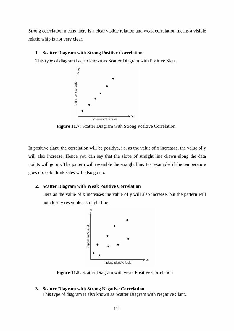
114

Strong correlation means there is a clear visible relation and weak correlation means a visible

relationship is not very clear.

1. Scatter Diagram with Strong Positive Correlation

This type of diagram is also known as Scatter Diagram with Positive Slant.

Figure 11.7: Scatter Diagram with Strong Positive Correlation

In positive slant, the correlation will be positive, i.e. as the value of x increases, the value of y

will also increase. Hence you can say that the slope of straight line drawn along the data

points will go up. The pattern will resemble the straight line. For example, if the temperature

goes up, cold drink sales will also go up.

2. Scatter Diagram with Weak Positive Correlation

Here as the value of x increases the value of y will also increase, but the pattern will

not closely resemble a straight line.

Figure 11.8: Scatter Diagram with weak Positive Correlation

3. Scatter Diagram with Strong Negative Correlation This type of diagram is also known as Scatter Diagram with Negative Slant.

115

Figure 11.9: Scatter Diagram with Strong Positive Correlation

In negative slant, the correlation will be negative, i.e. as the value of x increases, the value of

y will decrease. Here you can say that the slope of a straight line drawn along the data points

will go down. For example, if the temperature goes up, sales of entry tickets to the goes

down.

4. Scatter Diagram with Weak Negative Correlation

Here as the value of x increases the value of y will decrease, but the pattern will not resemble

a straight line.

Figure 11.10: Scatter Diagram with Weak Negative Correlation

11.1.6 Benefits of a Scatter Diagram

1. The following are a few advantages of a scatter diagram:

2. It shows the relationship between two variables.

3. It is the best method to show you a non-linear pattern.

4. The range of data flow, i.e. maximum and minimum value, can be easily determined.

116

5. Observation and reading is straightforward.

6. Plotting the diagram is relatively simple.

11.1.7 Limitations of a Scatter Diagram

The following are a few limitations of a scatter diagram:

� Scatter diagram is unable to give you the exact extent of correlation.

� Scatter diagram does not show you the quantitative measure of the relationship

between the variable. It only shows the quantitative expression of the quantitative

change.

� This chart does not show you the relationship for more than two variables.

11.1.8 Simple Bivariate Regression Model

A regression model may be simple (linear), multiple or linear. We shall consider the simple

Bivariate linear regression model, which is of the form:

exY ++= βα ……………………* Where

Y is the dependent variable

X is the independent variable α is the intercept

β is the slope of the line e is the error term

The equation * is referred to as Least Square Equation. However, both α and β are constants

and are determined by solving the simultaneous re-equations

∑∑ += xny βα…………………….(i)

∑ ∑ ∑+= 2xxxy βα………………(ii)

The two equations are the normal equations for the least square line. Solving the equations

simultaneously, the values of α andβ are obtained as: 2 2

ˆ( )

N xy x y

N x xβ

−=

−∑ ∑ ∑∑ ∑

, ˆˆ y xα β= −

Computationally, the slope could be calculated as 2 2ˆ

( )i i i i

i i

n x y x y

n x xβ

−=

−∑ ∑ ∑∑ ∑

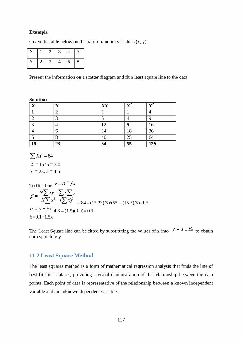
117

Example

Given the table below on the pair of random variables (x, y)

X 1 2 3 4 5

Y 2 3 4 6 8

Present the information on a scatter diagram and fit a least square line to the data Solution X Y XY X 2 Y2 1 2 2 1 4 2 3 6 4 9 3 4 12 9 16 4 6 24 18 36 5 8 40 25 64 15 23 84 55 129

∑ = 84XY

0.35/15 ==X 6.45/23 ==Y

To fit a line xy βα +=

∑ ∑∑ ∑ ∑

−−

=22 )( xxN

yxxyNβ

=(84 - (15.23)/5)/(55 – (15.5)/5)=1.5 xy βα −= 4.6 – (1.5)(3.0)= 0.1

Y=0.1+1.5x

The Least Square line can be fitted by substituting the values of x into xy βα += to obtain corresponding y

11.2 Least Square Method

The least squares method is a form of mathematical regression analysis that finds the line of

best fit for a dataset, providing a visual demonstration of the relationship between the data

points. Each point of data is representative of the relationship between a known independent

variable and an unknown dependent variable.

118

11.2.1 Breaking Down 'Least Squares Method'

The least squares method provides the overall rationale for the placement of the line of best

fit among the data points being studied.

The most common application of the least squares method, referred to as linear or ordinary,

aims to create a straight line that minimizes the sum of the squares of the errors generated by

the results of the associated equations, such as the squared residuals resulting from

differences in the observed value and the value anticipated based on the model.

This method of regression analysis begins with a set of data points to be graphed. An analyst

using the least squares method will be seeking a line of best fit that explains the potential

relationship between an independent variable and a dependent variable.

In regression analysis, dependent variables are designated on the vertical Y axis and

independent variables are designated on the horizontal X axis. These designations will form

the equation for the line of best fit, which is determined from the least squares method.

Example

The following are 8 data points that shows the relationship between the number of fishermen

and the amount of fish (in thousand pounds) they can catch a day.

Number of Fishermen Fish Caught

18 39

14 9

9 9

10 7

5 8

22 35

14 36

12 22

According to this data set, what is the function between the number of fishermen and the

amount of fish caught?

Hint: let the number of fisherman be x, and the amount of fish caught be y, and use LLS to

find the coefficients.

119

Answer

By the simple calculation and statistic knowledge, we can easily find out:

1. = 13

2. = 20.625, and 3. the following chart

X Y

18 39 5 18.375 91.875 25

14 9 1

1

9 9

46.5 16

10 7

40.875 9

5 8

101 64

22 35 9 14.375 129.375 81

14 36 1 15.375 15.375 1

12 22 1.375

1

Thus, we have , and , so the slope, a, = .

And last the intercept, b, = Therefore, the linear least-squares line is .The line of best fit

determined from the least squares method has an equation that tells the story of the

relationship between the data points.

Computer software models are used to determine the line of best fit equation, and these

software models include a summary of outputs for analysis. The least squares method can be

used for determining the line of best fit in any regression analysis. The coefficients and

summary outputs explain the dependence of the variables being tested.

Summary

In this study session you have learnt about: 1.Scatter Diagram

Scatter graph method is a graphical technique of separating fixed and variable components of

120

mixed cost by plotting activity level along x-axis and corresponding total cost (mixed cost)

along y-axis. A regression line is then drawn on the graph by visual inspection.

2.Least Square Method

The least squares method is a form of mathematical regression analysis that finds the line of

best fit for a dataset, providing a visual demonstration of the relationship between the data

points. Each point of data is representative of the relationship between a known independent

variable and an unknown dependent variable.






end of this Module.


Highlight on the Scatter Diagram Method


Discuss on the Least Square Method

Reference


Hall.




Publications

Shangodoyin D. K. et al (2002). Statistical Theory and Methods Ibadan: Joytal Press.

121

Study Session 12: Correlation Analysis

Introduction

Correlation is another way of assessing the relationship between variables. To be more

precise, it measures the extent of correspondence between the ordering of two

random variables. There is a large amount of resemblance between regression and

correlation but for their methods of interpretation of the relationship. For example, a

scatter diagram is of tremendous help when trying to describe the type of relationship existing

between two variables.

This study session introduces you to the concept of correlation. The definition and types of

correlation are highlighted. Interpretation of correlation coefficient is discussed. Examples

are given for the two types of correlation discussed.



12.1 Explain Pearson Product-Moment Correlation

12.2 Discuss Spear’s Ranking Order Correlation

12.1 Pearson Product Correlation

The Pearson product-moment correlation coefficient (or Pearson correlation coefficient, for

short) is a measure of the strength of a linear association between two variables and is

denoted by r. Basically, a Pearson product-moment correlation attempts to draw a line of best

fit through the data of two variables, and the Pearson correlation coefficient, r, indicates how

far away all these data points are to this line of best fit (i.e., how well the data points fit this

new model/line of best fit).

122

12.1.1 What values can the Pearson correlation coefficient take

The Pearson correlation coefficient, r, can take a range of values from +1 to -1. A value of 0

indicates that there is no association between the two variables. A value greater than 0

indicates a positive association; that is, as the value of one variable increases, so does the

value of the other variable. A value less than 0 indicates a negative association; that is, as the

value of one variable increases, the value of the other variable decreases. This is shown in the

diagram below:

Figure 12.1: Types of Pearson Correlation

12.1.2 How can we determine the strength of association based on the Pearson

correlation coefficient

The stronger the association of the two variables, the closer the Pearson correlation

coefficient, r, will be to either +1 or -1 depending on whether the relationship is positive or

negative, respectively. Achieving a value of +1 or -1 means that all your data points are

included on the line of best fit – there are no data points that show any variation away from

this line.

Values for r between +1 and -1 (for example, r = 0.8 or -0.4) indicate that there is variation

around the line of best fit. The closer the value of r to 0 the greater the variation around the

line of best fit. Different relationships and their correlation coefficients are shown in the

diagram below:

123

Figure 12.2: Pearson correlation coefficient

12.1.3 Guidelines to interpreting Pearson's correlation coefficient

Yes, the following guidelines have been proposed:

Coefficient, r

Strength of Association Positive Negative

Small .1 to .3 -0.1 to -0.3

Medium .3 to .5 -0.3 to -0.5

Large .5 to 1.0 -0.5 to -1.0

Remember that these values are guidelines and whether an association is strong or not will

also depend on what you are measuring.

12.1.4 Using any type of Variable for Pearson's Correlation Coefficient

No, the two variables have to be measured on either an interval or ratio scale. However, both

variables do not need to be measured on the same scale (e.g., one variable can be ratio and

one can be interval). Further information about types of variable can be found in our Types of

Variable guide. If you have ordinal data, you will want to use Spearman's rank-order

correlation or a Kendall's Tau Correlation instead of the Pearson product-moment correlation.

12.1.5 Do the two variables have to be measured in the same units

No, the two variables can be measured in entirely different units. For example, you could

correlate a person's age with their blood sugar levels. Here, the units are completely different;

age is measured in years and blood sugar level measured in mmol/L (a measure of

124

concentration).

Indeed, the calculations for Pearson's correlation coefficient were designed such that the units

of measurement do not affect the calculation. This allows the correlation coefficient to be

comparable and not influenced by the units of the variables used.

12.1.6 What about dependent and independent variables

The Pearson product-moment correlation does not take into consideration whether a variable

has been classified as a dependent or independent variable. It treats all variables equally. For

example, you might want to find out whether basketball performance is correlated to a

person's height. You might, therefore, plot a graph of performance against height and

calculate the Pearson correlation coefficient.

Lets say, for example, that r = .67. That is, as height increases so does basketball

performance. This makes sense. However, if we plotted the variables the other way around

and wanted to determine whether a person's height was determined by their basketball

performance (which makes no sense), we would still get r = .67.

This is because the Pearson correlation coefficient makes no account of any theory behind

why you chose the two variables to compare. This is illustrated below:

Figure 12.3: Comparison of Two Pearson Variables

12.1.7 The Pearson correlation coefficient indicate the slope of the line

It is important to realize that the Pearson correlation coefficient, r, does not represent the

slope of the line of best fit. Therefore, if you get a Pearson correlation coefficient of +1 this

125

does not mean that for every unit increase in one variable there is a unit increase in another. It

simply means that there is no variation between the data points and the line of best fit. This is

illustrated below:

Figure 12.4: Pearson correlation coefficient indicate the slope of the line

12.1.8 Assumptions of Pearson's correlation make

There are five assumptions that are made with respect to Pearson's correlation:

1. The variables must be either interval or ratio measurements (see our Types of

Variable guide for further details).

2. The variables must be approximately normally distributed (see our Testing for

Normality guide for further details).

3. There is a linear relationship between the two variables (but see note at bottom of

page). We discuss this later in this guide (jump to this section here).

4. Outliers are either kept to a minimum or are removed entirely. We also discuss this

later in this guide (jump to this section here).

5. There is homoscedasticity of the data. This is discussed later in this guide (jump to

this section here).

12.1.9 How can you detect a linear relationship

To test to see whether your two variables form a linear relationship you simply need to plot

them on a graph (a scatte rplot, for example) and visually inspect the graph's shape. In the

diagram below, you will find a few different examples of a linear relationship and some non-

linear relationships. It is not appropriate to analyse a non-linear relationship using a Pearson

product-moment correlation.

126

Figure 12.5: Pearson linear relationship

Note: Pearson's correlation determines the degree to which a relationship is linear. Put

another way, it determines whether there is a linear component of association between two

continuous variables. As such, linearity is not actually an assumption of Pearson's correlation.

However, you would not normally want to pursue a Pearson's correlation to determine the

strength and direction of a linear relationship when you already know the relationship

between your two variables is not linear.

Instead, the relationship between your two variables might be better described by another

statistical measure. For this reason, it is not uncommon to view the relationship between your

two variables in a scatter plot to see if running a Pearson's correlation is the best choice as a

measure of association or whether another measure would be better.

In Text Question

To test to see whether two variables form a linear relationship you simply need to plot them

on a table.True/False

In Text Answer

False (Graph)

12.2 Spear’s Ranking Order Correlation

In statistics, a rank correlation is any of several statistics that measure an ordinal association

the relationship between rankings of different ordinal variables or different rankings of the

same variable, where a "ranking" is the assignment of the labels "first", "second", "third", etc.

to different observations of a particular variable.

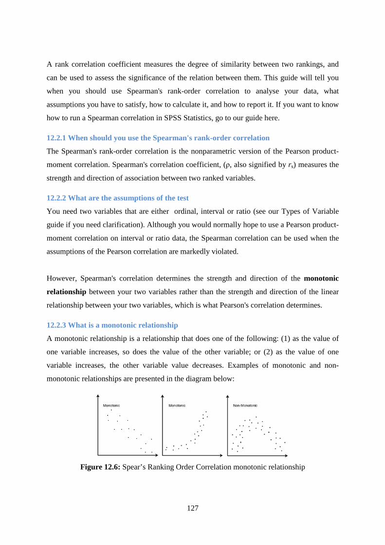
127

A rank correlation coefficient measures the degree of similarity between two rankings, and

can be used to assess the significance of the relation between them. This guide will tell you

when you should use Spearman's rank-order correlation to analyse your data, what

assumptions you have to satisfy, how to calculate it, and how to report it. If you want to know

how to run a Spearman correlation in SPSS Statistics, go to our guide here.

12.2.1 When should you use the Spearman's rank-order correlation

The Spearman's rank-order correlation is the nonparametric version of the Pearson product-

moment correlation. Spearman's correlation coefficient, (ρ, also signified by rs) measures the

strength and direction of association between two ranked variables.

12.2.2 What are the assumptions of the test

You need two variables that are either ordinal, interval or ratio (see our Types of Variable

guide if you need clarification). Although you would normally hope to use a Pearson product-

moment correlation on interval or ratio data, the Spearman correlation can be used when the

assumptions of the Pearson correlation are markedly violated.

However, Spearman's correlation determines the strength and direction of the monotonic

relationship between your two variables rather than the strength and direction of the linear

relationship between your two variables, which is what Pearson's correlation determines.

12.2.3 What is a monotonic relationship

A monotonic relationship is a relationship that does one of the following: (1) as the value of

one variable increases, so does the value of the other variable; or (2) as the value of one

variable increases, the other variable value decreases. Examples of monotonic and non-

monotonic relationships are presented in the diagram below:

Figure 12.6: Spear’s Ranking Order Correlation monotonic relationship

128

12.2.4 Why is a monotonic relationship important to Spearman's correlation

Spearman's correlation measures the strength and direction of monotonic association between

two variables. Monotonicity is "less restrictive" than that of a linear relationship. For

example, the middle image above shows a relationship that is monotonic, but not linear.

A monotonic relationship is not strictly an assumption of Spearman's correlation. That is, you

can run a Spearman's correlation on a non-monotonic relationship to determine if there is a

monotonic component to the association.

However, you would normally pick a measure of association, such as Spearman's correlation,

that fits the pattern of the observed data. That is, if a scatterplot shows that the relationship

between your two variables looks monotonic you would run a Spearman's correlation because

this will then measure the strength and direction of this monotonic relationship.

On the other hand if, for example, the relationship appears linear you would run a Pearson's

correlation because this will measure the strength and direction of any linear relationship.

You will not always be able to visually check whether you have a monotonic relationship, so

in this case, you might run a Spearman's correlation anyway.

12.2.5 How to rank data

In some cases your data might already be ranked, but often you will find that you need to

rank the data yourself. Thankfully, ranking data is not a difficult task and is easily achieved

by working through your data in a table. Let us consider the following example data

regarding the marks achieved in a maths and English exam:

Exam Marks

English 56 75 45 71 61 64 58 80 76 61

Maths 66 70 40 60 65 56 59 77 67 63

The procedure for ranking these scores is as follows:

First, create a table with four columns and label them as below:

English (mark) Maths (mark) Rank (English) Rank (maths) 56 66 9 4

75 70 3 2

45 40 10 10

129

English (mark) Maths (mark) Rank (English) Rank (maths) 71 60 4 7

61 65 6.5 5

64 56 5 9

58 59 8 8

80 77 1 1

76 67 2 3

61 63 6.5 6

You need to rank the scores for maths and English separately. The score with the highest

value should be labelled "1" and the lowest score should be labelled "10" (if your data set has

more than 10 cases then the lowest score will be how many cases you have). Look carefully

at the two individuals that scored 61 in the English exam (highlighted in bold).

Notice their joint rank of 6.5. This is because when you have two identical values in the data

(called a "tie"), you need to take the average of the ranks that they would have otherwise

occupied. We do this because, in this example, we have no way of knowing which score

should be put in rank 6 and which score should be ranked 7. Therefore, you will notice that

the ranks of 6 and 7 do not exist for English. These two ranks have been averaged ((6 + 7)/2

= 6.5) and assigned to each of these "tied" scores.

12.2.6 What is the definition of Spearman's rank-order correlation?

There are two methods to calculate Spearman's correlation depending on whether: (1) your

data does not have tied ranks or (2) your data has tied ranks. The formula for when there are

no tied ranks is:

where di = difference in paired ranks and n = number of cases. The formula to use when there

are tied ranks is:

130

where i = paired score.

It is denoted by

∑∑∑

−−

−=

))(( 2222 YnYXnX

YXnXYr

= -1 ≤ r ≤ 1

Example: The demand and price of a particular commodity are recorded as follows:

Demand (Y) 2 3 5 4 6

Price N(X) 1 2 3 4 5

Find the product moment correlation co-efficient of the data.

Solution

Y i X i X i Yi 2iX

Y2

2 1 2 1 4

3 2 6 4 9

5 3 15 9 25

4 4 16 16 16

6 5 30 25 36

20 15 96 55 90

∑∑∑

−−

−=

))(( 2222 YnYXnX

YXnXYr

= ( )[ ]( )[ ]23 4(590)3(555

)4)(3(590

−−

−

9.010

9

1010

9 ===x

r

The above result r = 0.9 implies a strong (or direct) relationship (Correlation between) the

price and demand for the commodity.

Interpretation of r

i. When r = 1, it indicates a perfect positive correlation.

ii. When r = -1, it indicates a perfect negative correlation.

131

iii. When –1 < r < -0.5, it indicates a strong negative correlation.

iv. When –0.5 < r < 0, it indicates a weak negative correlation.

v. When 0 < r < 0.5, it indicates a weak positive correlation.

vi. When 0.5 < r 1, it indicates a strong positive correlation.

Example

Suppose we are interested in seeing if there is a linear relationship between age and

height for children ages 3 to 9.

A random sample of children gave the following data

Age (x) Height (y) xy

3 38 114

3 31 93

4 37 148

6 40 240

6 49 294

7 45 315

9 51 459

38 291 1663

So

3 8 , 2 9 1 , 1 6 6 3x y x y= = =∑ ∑ ∑

Furthermore,

∑ = 2362x ,and ∑ = 124012y

Response variable (y) - the one we are primarily interested in.

Explanatory variable (x) - one that is thought to affect the response variable.

First, construct a scatter diagram (scatterplot) - a plot of the ordered pairs (x, y) with

the response variable, y, on the vertical axis.

Correlation coefficient - measures the strength and direction of the linear relationship

between two quantitative variables.

Notation: � = population correlation

r = sample correlation

132

( )( )( ) ( )∑ ∑∑ ∑

∑ ∑∑−−

−=

2222 yynxxn

yxxynr

So, for our data set,

( ) ( )( )( ) ( ) ( ) ( )2 2

7 1 6 6 3 3 8 2 9 10 . 8 7 7

7 2 3 6 3 8 7 1 2 4 0 1 2 9 1r

−= =

− −

Interpretation : There is a strong, positive linear relationship between age and height for

children ages 3 to 9.

Coefficient of determination = r2 = the proportion of variation in y that is explained by

its linear relationship with x.

1

Interpretation : 76.9% of the variation in height can be explained by its linear

relationship with age.

Summary

In this study session you have learnt about: 1. Pearson Product Correlation

The Pearson product-moment correlation coefficient (or Pearson correlation coefficient, for

short) is a measure of the strength of a linear association between two variables and is

denoted by r.

Basically, a Pearson product-moment correlation attempts to draw a line of best fit through

the data of two variables, and the Pearson correlation coefficient, r, indicates how far away

all these data points are to this line of best fit (i.e., how well the data points fit this new

model/line of best fit).

133

1. Spear’s Ranking Order Correlation In statistics, a rank correlation is any of several statistics that measure an ordinal association

the relationship between rankings of different ordinal variables or different rankings of the

same variable, where a "ranking" is the assignment of the labels "first", "second", "third", etc.

to different observations of a particular variable.






end of this Module.


Highlight on Pearson Product Correlation


Discuss Spear‘s Ranking order Correlation

Reference

John, E. F.(1974). Modern Elementary Statistics, International Editions London: Prentice

Hall

Murray, R. S. (1972) Schaum’s Outline Series. Theory and Problems of Statistics. New York:

McGraw-Hill Book Company.


Publications.

134

Study Session 13: Introduction to Time Series Analysis

Introduction

A time series plays a significant role in the analysis of socio-economic data. These are mostly

data on finance, insurance, marketing, population, etc. It is also very useful in forecasting

because the objective of a time series is to forecast future values to enable us make good

plans for the future.

A time series is a series of data points indexed (or listed or graphed) in time order. Most

commonly, a time series is a sequence taken at successive equally spaced points in time. ...

Time series forecasting is the use of a model to predict future values based on previously

observed values.

The concept of Time Series is covered in this study session. It introduces you to the definition

of Time Series, objectives of a Time Series, component of a Time Series and models of Time

Series.



13.1 Define Time Series

13.2 Component of Time Series

13.1 Definition of a Time Series

A time series consists of a set of chronological observation (continuous or discrete) taken at a

specified time, usually at equal intervals. We denote a time series by (Xt) where (Xt) is the

observed value in time.

A time series may be represented graphically as a plot, that is, the plot of observation Xt

against time (t) so as to observe the inherent characteristics of the time series data. The basic

idea of time series is that given a set of data, one should be able to estimate or forecast Xt+1,

Xt+2, etc.

135

13.1.1 Objectives of Time Series Analysis

It would be incomplete to approach the fundamentals of time series analysis without

discussing the main reasons for analyzing time series. The objectives of time series analysis

may be broadly classified into four major types of investigation.

The first exploration of time series data is the plot of the series over time (Time Plot), then a

sample descriptive measures of the main properties of the series could be obtained. In this,

we intend to look at outliers, troughs, presence of turning points etc that may be pronounced

on the time plot.

1. In order to have a deeper understanding of the mechanism, which generates a given

time series, we make use of the variation in one time series to explain the variation in

another time series. The analysis of linear systems provides more information.

2. An important task in time series analysis is to predict the future. Given an observed

time series, one may want to predict the future values of the series. If one can forecast

that a manufacturing process is going to move off target, then an appropriate

corrective action could be taken.

3. When a time series generated measures the quality of a manufacturing process, the

aim of the analysis may be to control the process. The procedures on these are of

several kinds, ranging from charts to inspection models. A stochastic model is fitted

to the series, and the future values of the series are provided and then the input

process variables are adjusted so as to keep the process on target.

13.2 Components of Time Series

The factors that are responsible to bring about changes in a time series, also called the

components of time series, are as follows:

Figure 13.1:

1.Secular Trend

The secular trend is the main component of a time series which results from long term effect

of socio-economic and political factors. This trend may show the growth or decline in a time

series over a long period. This is the type of tendency which continues to persist for a

long period. Prices, export and imports data, for example, reflect obviously increasing

tendencies over time.

2.Seasonal Trend

These are short term movements occurring in a data due to seasonal factors. The short term is

generally considered as a period in which changes occur in a time series with variations in

weather or festivities. For example, it is commonly observed that the consumption of ice

cream during summer us generally high and hence sales of an ice

higher in some months of the year while relatively lower during winter months.

Employment, output, export etc. are subjected to change due to variation in weather.

Similarly sales of garments, umbrella, greeting cards and fire

variation during festivals like Valentine’s Day, Eid, Christmas, New Year etc. These types of

variation in a time series are isolated only when the series is provided bi

monthly.

136

Figure 13.1:Component of Time Series

is the main component of a time series which results from long term effect

economic and political factors. This trend may show the growth or decline in a time

series over a long period. This is the type of tendency which continues to persist for a



riod in which changes occur in a time series with variations in

weather or festivities. For example, it is commonly observed that the consumption of ice

cream during summer us generally high and hence sales of an ice-cream dealer would be

onths of the year while relatively lower during winter months.


Similarly sales of garments, umbrella, greeting cards and fire-work are subjected to large

g festivals like Valentine’s Day, Eid, Christmas, New Year etc. These types of

variation in a time series are isolated only when the series is provided biannually, quarterly or

is the main component of a time series which results from long term effect

economic and political factors. This trend may show the growth or decline in a time

series over a long period. This is the type of tendency which continues to persist for a very



riod in which changes occur in a time series with variations in

weather or festivities. For example, it is commonly observed that the consumption of ice-

cream dealer would be

onths of the year while relatively lower during winter months.


work are subjected to large

g festivals like Valentine’s Day, Eid, Christmas, New Year etc. These types of

annually, quarterly or

137

3.Cyclic Movements

These are long term oscillation occurring in a time series. These oscillations are mostly

observed in economics data and the periods of such oscillations are generally extended from

five to twelve years or more. These oscillations are associated to the well known business

cycles. These cyclic movements can be studied provided a long series of measurements, free

from irregular fluctuations is available.

4.Irregular Fluctuations

These are sudden changes occurring in a time series which are unlikely to be repeated, it is

that component of a time series which cannot be explained by trend, seasonal or cyclic

movements .It is because of this fact these variations some-times called residual or random

component.

These variations though accidental in nature, can cause a continual change in the trend,

seasonal and cyclical oscillations during the forthcoming period. Floods, fires, earthquakes,

revolutions, epidemics and strikes etc,. are the root cause of such irregularities.

In Text Question

The short term is generally considered as a period in which changes occur in a time series

with variations in weather or festivities.

(a) Irregular

(b) Cyclic Movement

(c) Seasonal Trend

(d) Secular Trend

In Text Answer

The answer is (c) seasonal Trend

13.2.1 Time series decomposition

We shall think of the time series ytyt as comprising three components: a seasonal component,

a trend-cycle component (containing both trend and cycle), and a remainder component

(containing anything else in the time series). For example, if we assume an additive model,

then we can write

138

yt=St+Tt+Et,yt=St+Tt+Et,

where ytyt is the data at period tt, StSt is the seasonal component at period tt, TtTt is the

trend-cycle component at period tt and EtEt is the remainder (or irregular or error)

component at period tt. Alternatively, a multiplicative model would be written as

yt=St×Tt×Et.yt=St×Tt×Et.

The additive model is most appropriate if the magnitude of the seasonal fluctuations or the

variation around the trend-cycle does not vary with the level of the time series. When the

variation in the seasonal pattern, or the variation around the trend-cycle, appears to be

proportional to the level of the time series, then a multiplicative model is more appropriate.

With economic time series, multiplicative models are common.

An alternative to using a multiplicative model, is to first transform the data until the variation

in the series appears to be stable over time, and then use an additive model.

Sometimes, the trend-cycle component is simply called the “trend” component, even though

it may contain cyclic behaviour as well.

The data have been adjusted by working days and normalized so a value of 100 corresponds

to 2005.

Figure 13.2: Time series Decomposition 1

139

13.2.2 De-Seasonalizing a Time Series

Seasonality in a time series can be identified by regularly spaced peaks and troughs which

have a consistent direction and approximately the same magnitude every year, relative to the

trend. The graph below, that of a retailer, shows a strongly seasonal series. In the fourth

quarter each year, sales increase due to holiday shopping. In this example, the magnitude of

the seasonal component increases over time, as does the trend.

Figure 13.3: Time series Decomposition 2

A time series can be de-seasonalized when only a seasonal component is present, or when

both seasonal and trend components are present. This is a two-step process:

1.Compute seasonal/irregular indexes and use them to de-seasonalize the data;

2.Use regression analysis on the remaining trend data if a trend is apparent in

13.2.3 Seasonal Variation

In statistics, many time series exhibit cyclic variation known as seasonality, seasonal

variation, periodic variation, or periodic fluctuations. This variation can be either regular or

semi-regular. Seasonal variation is a component of a time series which is defined as the

repetitive and predictable movement around the trend line in one year or less.

It is detected by measuring the quantity of interest for small time intervals, such as days,

weeks, months or quarters. Organizations facing seasonal variations, like the motor vehicle

140

industry, are often interested in knowing their performance relative to the normal seasonal

variation.

The same applies to the ministry of employment which expects unemployment to increase in

June because recent graduates are just arriving into the job market and schools have also been

given a vacation for the summer. That unemployment increased as predicted is a moot point;

the relevant factor is whether the increase is more or less than expected.

13.2.4 Moving Average

A widely used indicator in technical analysis that helps smooth out price action by filtering

out the “noise” from random price fluctuations. A moving average (MA) is a trend-following

or lagging indicator because it is based on past prices.

The two basic and commonly used MAs are the simple moving average (SMA), which is the

simple average of a security over a defined number of time periods, and the exponential

moving average (EMA), which gives bigger weight to more recent prices.

The most common applications of MAs are to identify the trend direction and to determine

support and resistance levels. While MAs are useful enough on their own, they also form the

basis for other indicators such as the Moving Average Convergence Divergence (MACD).

13.2.5 Additive model

A data model in which the effects of individual factors are differentiated and added together

to model the data. They occur in several Minitab commands:

• An additive model is optional for Decomposition procedures and for Winters' method.

• An additive model is optional for two-way ANOVA procedures. Choose this option to

omit the interaction term from the model.

13.2.6 Multiplicative model

This model assumes that as the data increase, so does the seasonal pattern. Most time series

plots exhibit such a pattern. In this model, the trend and seasonal components are multiplied

and then added to the error component.

141

13.2.7 Using an additive model or a multiplicative model

Choose the multiplicative model when the magnitude of the seasonal pattern in the data

depends on the magnitude of the data. In other words, the magnitude of the seasonal pattern

increases as the data values increase, and decreases as the data values decrease.

Choose the additive model when the magnitude of the seasonal pattern in the data does not

depend on the magnitude of the data. In other words, the magnitude of the seasonal pattern

does not change as the series goes up or down.

If the pattern in the data is not very obvious, and you have trouble choosing between the

additive and multiplicative procedures, you can try both and choose the one with smaller

accuracy measures.

Time Series Models

In the light of the above components of a time series {Xt}, we can represent a series in two

convenient models as some functions of the component. The standard forms are the

following:

1. Xt = Tt + Ct + St + It. called the additive model an

2. Xt = Tt . Ct . St . It. called the multiplicative model.

The logarithmic transformation of (1) leads to (2), and where the cyclic variation is not

pronounced, the two models reduce to Xt = Tt . Ct . It. and Tt + Ct + It respectively.

Summary

In this study session you have learnt about: 1. Definition of a Time Series

A time series consists of a set of chronological observation (continuous or discrete) taken at a

specified time, usually at equal intervals. We denote a time series by (Xt) where (Xt) is the

observed value in time. A time series may be represented graphically as a plot, that is, the

plot of observation Xt against time (t) so as to observe the inherent characteristics of the time

series data.

2.Component of Time Series

� Secular Trend

� Seasonal Trend

142

� Cyclic Movements

� Irregular Fluctuations






end of this Module.


Explain Time Series


Discuss the Component of Time Series

References


Publications.

Shangodoyin D. K. and Ojo, J. F. (200). Elements of Time Series Analysis Ibadan: Rasmed

Publications.

Shangodoyin D. K. et al (2002). Statistical Theory and Methods Ibadan: Joytal Printing Press.

143

Study Session 14: Time Series Analysis - Estimation of Trends

and Seasonal Variations

Introduction

Trend estimation is a statistical technique to aid interpretation of data. When a series of

measurements of a process are treated as a time series, trend estimation can be used to make

and justify statements about tendencies in the data, by relating the measurements to the times

at which they occurred.

The objective of time series analysis is to identify the direction and magnitude of any trend

present in the data. To achieve this objective, many methods are available in practice for the

estimation of trend in a series. We shall examine some of these methods

Figure 14.1: Estimation Trend

This study session will introduce you to estimation of trends and seasonal variation in time

series analysis.

144



14.1 Highlight on Moving Average Method

14.2 Explain The Least Square Method

14.1 Moving Average Method

The technique of using the moving average method is to replace a particular measurement by

the arithmetic mean of a series of measurements of which it is the center. When an odd

number is chosen, the moving average is centred as an observed measurement.

But where an even number of measurement is chosen, the moving average is centred between

two observed measurements and must be re-centred before comparisons can be made

between the average and the measurement.

Suppose we are given X1, X2, ….,XN on {Xt}, the n-point moving average are:

Y1 = X1+ X2+ ….+ XN

n

Y2 = X1+ X2+ ….+ XN

n

. .

YN-n = XN-n + XN-n + ….+ XN

n

For illustration, consider the hypothetical observations X1, X2,…,X12 given on {Xt}. Suppose

our interest is on 4pt-moving average, we shall make use of the routine displayed in the table

below:

DATA 4-POINT TOTAL

4-POINT AVERAGE CENTRED 4-POINT MOVING AVERAGE

X1 4

145

X2

X3

X4

X5

X6

X7

X8

X9

X10

X11

X12

∑ Xi = T1 i=1

5

∑ Xi = T2 i=2

6

∑ Xi = T3 i=3

7

∑ Xi = T4 i=4

8

∑ Xi = T5 i=5

9

∑ Xi = T6 i=6

10

∑ Xi = T7 i=7

11

∑ Xi = T8 i=8

12

∑ Xi = T9 i=9

T1/4 = V1

T2/4 = V2

T3/4 = V3

T4/4 = V4

T5/4 = V5

T6/4 = V6

T7/4 = V7

T8/4 = V8

T9/4 = V9

V1 + V2 = M1

V2 + V3 = M2

V3 + V4 = M3

V4 + V5 = M4

V5 + V6 = M5

V6 + V7 = M6

V7 + V8 = M7

V8 + V9 = M8

The advantage is that it gives the true nature of the trend, that is, a simple description of the

underlying trend, particularly, when the trend is small. Although, this method loses the

extreme values, it should be noted that one can generalize the moving average trend for the

series to any point in time.

146

14.2 Method of Least Squares

This method can be used to find the equation of an appropriate trend line and the trend values

Tt can be computed from the equation using the least squares approach of regression analysis.

The normal equations for the trend line are:

∑∑==

+=n

t

n

tt tbnaX

11

∑∑∑===

+=n

t

n

t

n

tt tbtatX

1

2

11

The least squares estimate of a and b are the solution to the normal equations which can

be determined by solving the equations simultaneously. The estimates are then given as

tbXa t −=ˆ

∑ ∑

∑ ∑∑

−

−=

n

tt

n

XttX

b

tt

22 )(

))((

Thus the trend line equation is then

tbaTtˆˆ +=

One disadvantage of this method is that a linear trend may be fitted into a series which is not

exactly linear.

14.2.1 The Freehand Method

This consists of fitting a trend line or curve by looking at the graph. If the type of equation of

this curve is known, it is possible to obtain the constants in the equation by choosing as many

points on the curve in a straight line; two points are necessary. The disadvantage of this

method is that different observers will obtain different curves and equations.

14.2.2 The Method of Semi Average

This consists of separating the data into two equal parts and averaging the data in each part,

thus obtaining two points on the graph of the time series. A trend line is then drawn between

147

these two points, and trend values can be determined. The demerit of this method is that it

may lead to poor results when used indiscriminately. Also, it is applicable only where the

trend is linear.

14.2.3 The Method of Curve Fitting

This approach is particularly adequate when the series is non-seasonal and has trend. The

various curves that can be fitted are Gompertz, Logistic and Polynomial.

1.Elimination of Trend

A special way of eliminating trend is through filtering (which is particularly useful for

removing a trend). This is done to make a series stationary, the approach is by differencing

the data based on the nature of the curve.For non-seasonal data, first-order differencing is

sufficient to attain stationary, so that a new series is generated. Suppose we have a linear

curve given as:

xt = a + bt

To remove trend we make use of the first difference defined as:

Yt = ∆ xt = xt – xt-1

= a + bt – (a + bt – b)

= b. Constant and independent of time.

Thus in general to eliminate the nth order polynomial trend we use

n xt

14.2.4 Estimation of Seasonal Variation

A. Multiplicative Model

Suppose we assume a multiplicative model of the form

Xt = Tt . St . Ct . It or

Xt = Tt(Ct) . St . It

Having estimated the trend, the seasonal variation at time t is

St = Xt / Tt

B. Additive Model

Suppose a series Xt has an additive relationship with the time series components, that is,

Xt = Tt + St + Ct + It or

148

Xt = Tt(Ct) + St + It

Then the seasonal variation at time t is

St = Xt - Tt

Example 1

The time series shown below shows the cost of production of Associated Matches Industry

for a four-year period, spanning 1988 - 1992.

cost of production (_’000s) of ami

Year I

II

III

IV

1988

55.8

53.6

1989

55.5

57.5

57.2

54.6

1990

56.3

56

55.4

50.4

1991

56.1

57.5

53.9

53.4

1992

60.1

63

By using the method of moving averages, calculate the trend of the production cost. Plot both

sets of figures on a graph.

Solution

Year

Quarter

(i) Costs

(ii) 4-quarter Totals

(iii) 4-quarter total in pairs

(iv) Trend (iii�8)

1988

1989

1990

III

IV

I

II

III

IV

I

II

55.8

53.6

55.5

57.5

57.2

54.6

56.3

56

222.4

223.8

224.8

225.6

224.1

222.3

218.1

446.2

448.6

450.4

449.7

446.4

440.4

55.8

56.1

56.3

56.2

55.8

55.1

149

1991

1992

III

IV

I

II

III

IV

I

II

55.4

50.4

56.1

57.5

53.9

53.4

60.1

63

217.9

219.4

217.9

220.9

224.9

230.4

436

437.3

437.3

438.8

445.8

455.3

54.5

54.7

54.7

54.9

55.7

56.9

Fig. 1-1: Graph of cost of production of AMI (1988 - 1992) and its corresponding trend

values using moving averages method

Summary


1. Moving Average Method

The technique of using the moving average method is to replace a particular

measurement by the arithmetic mean of a series of measurements of which it is the

center. When an odd number is chosen, the moving average is centred as an observed

measurement.

But where an even number of measurement is chosen, the moving average is centred

50

52

54

56

58

60

62

64

88:3 89:1 89:3 90:1 90:3 91:1 91:3 92:1

COST

150

between two observed measurements and must be re-centred before comparisons can

be made between the average and the measurement.

2. Method of Least Squares

This method can be used to find the equation of an appropriate trend line and the trend

values Tt can be computed from the equation using the least squares approach of

regression analysis. The normal equations for the trend line are:

∑∑==

+=n

t

n

tt tbnaX

11

∑∑∑===

+=n

t

n

t

n

tt tbtatX

1

2

11

The least squares estimate of a and b are the solution to the normal equations which can

be determined by solving the equations simultaneously. The estimates are then given as

tbXa t −=ˆ

∑ ∑

∑ ∑∑

−

−=

n

tt

n

XttX

b

tt

22 )(

))((






end of this Module.


Explain moving average Method


Discuss Least Square Method

151

References

John, E. F.(1974). Modern Elementary Statistics. International Edition. London: Prentice

Hall

Murray, R. S. (1972 ) Schaum’s Outline Series. Theory and Problems of Statistics. New



Publications.

Shangodoyin D. K. and Ojo, J. F. (200). Elements of Time Series Analysis Ibadan: Rasmed

Publications.

152

Study Session 15: Time Series Analysis - Seasonal Indices and

Forecasting

Introduction

A seasonal index is a measure of how a particular season compares with the average season.

Seasonal indices are calculated so that their average is 1. This means that the sum of the

seasonal indices equals the number of seasons. To calculate de-seasonalised data, each entry

is divided by its seasonal index as follows.

Learning Outcomes From Study Session 15

15.1 Define Forecasting

15.2 Explain Elementary Forecasting

15.1 Define Forecasting

A planning tool that helps management in its attempts to cope with the uncertainty of the

future, relying mainly on data from the past and present and analysis of trends. Forecasting

starts with certain assumptions based on the management experience, knowledge, and

judgment.

These estimates are projected in the coming months or years using one or more techniques

such as Box-Jenkins models, Delphi method, exponential smoothing, moving averages,

regression analysis, and trend projection. Since any error in the assumptions will result in a

similar or magnified error in forecasting, the technique of sensitivity analysis is used which

assigns a range of values to the uncertain factors (variables).

15.1.1 Seasonal Indices

This is a set of numbers that shows the relative values of a variable during the months of the

year or quarters of a year. A suitable method is the Average Percentage Method; this method

153

involves the expression of the data as percentages of the total for the period. The percentages

for the corresponding months (quarters) of different years are then averaged, using either a

mean or median (If the mean is used, it helps to avoid extreme values, which may occur).

The resulting 12(4) percentages give the seasonal index. Depending on the model used, the

resulting total should be 1200% or 0% for multiplicative model, and 400% for additive

model. But if this is not so, a suitable factor should be used to adjust.

Consider the hypothetical figure (Xij) on quarterly sales in a company for four years:

Quarter YEAR 1 2 3 4

1997

1998

1999

2000

TOTAL

Average

X11 (S1)

X21 (S5)

X31 (S9)

X41 (S13)

S1+S5+S9+S13= ST1

ST1 x 100 = SI1

4

X12 (S2)

X22 (S6)

X32 (S10)

X42 (S14)

S2+S6+S10+S14 =ST2

ST2 x 100 = SI2

4

X13 (S3)

X23 (S7)

X33 (S11)

X43 (S15)

S3+S7+S11+S15 = ST3

ST3 x 100 = SI3

4

X14 (S4)

X24 (S8)

X34 (S12)

X44 (S16)

S4+S8+S12+S16 = ST4

ST4 x 100 = SI4

4

15.2 Elementary Forecasting

Very often, we have a series of measurements, which are affected by the same time series

components, such as trend and seasonal variation; these are accounted for in forecasting. Any

change in the more sensitive series will anticipate the corresponding change in the

components therein, and can be used as a forecasting indicator.

Generally, the forecasting for period p is

Xp = Tp x SIp and

Xp = Tp + SIp for both the multiplication and additive models respectively.

154

Example 1 The following information has been supplied by the sales department

1990

1991

Value of sales

First

8

20

40

Second

30

50

62

Third

60

80

92

Fourth

24

20

40

a. Using an additive model, find the centred moving average trend.

b. Find the average seasonal variation for each quarter.

c. Predict sales for the last quarter of 1992 and the first quarter of 1993

Solution 1.

Year

Quarter

(i)

Sales

(ii)

4-point

Moving

Average

(iii)

Centred

Moving

Average

(iv)

(i) - (iii)

1989

4

24

1990

1

8

30.5

2

30

30

0

29.5

3

60

31

29

32.5

4

20

35

-15

155

37.5

1991

1

20

40

-20

42.5

2

50

45

5

47.5

3

80

50

30

52.5

4

40

54

-14

55.5

1992

1

40

57

-17

58.5

2

62

3

92

2. The difference between the actual sales and the trend is in column (iv) of the table. By

averaging the appropriate quarterly values, an estimate of the ‘seasonal’ factors may

be obtained.

Quarter 1 ½(-20+(-17)) = -18.5

Quarter 2 ½(0+5) = 2.5

Quarter 3 ½(29+30) = 29.5

Quarter 4 ½(-15+(-14)) = -14.5

As these four values do not sum to zero (as they should using an additive model), they

may be corrected by adding 0.25 to each value to give:

-18.25; 2.75; 29.75; -14.25

3. An upward trend in the data is obvious and to predict future sales, this trend must be

extrapolated. The trend does not seem to be completely regular and without more

complicated analysis (e.g. fitting a linear trend to the data by a process of least

156

squares), the average quarterly increase in the trend seems to be approximately

4. On the basis of the last trend value (57) the predicted trend should be:

1992 - Quarter 4: 57 + 3 x 4 = 69

1993 - Quarter 1: 57 + 4 x 4 = 73

This gives actual sales estimates of:

69 - 14.25 = 54.75 i.e 55

and 73 - 18.25 = 54.75 i.e. 55

Example 2 The following data are the production of coca (‘000 tons) in Nigeria for the year 1988 to 2002:

YEAR 1988 1989 1990 1991 1992 1993 1994

Production (‘000) 4 3 4 5 9 9 15

YEAR 1996 1997 1998 1999 2000 2001 2002

Production (‘000) 10 26 17 18 35 24 40

a. Using the least square method, fit the linear trend

Y = a + bT, where T = t - 8

b. Calculate the trend value for each year.

c. Predict the production for 2003, using the fitted trend.

Solution a.

T -7 -6 -5 -4 -3 -2 -1 0 1 2 3 4 5 6 7

Production(Y) (‘000)

4 3 4 5 9 9 15 10 26 17 18 31 35 24 40

T2 49 36 25 16 9 4 1 0 1 4 9 16 25 36 49

TY -28 -18 -20 -20 -27 -18 15 0 26 34 54 124 175 144 280

∑ T = 0, ∑ Y=260, ∑ T2=280, ∑ TY=751 â = 260/15 = 17.30, b = 751/280 = 2.68

The required equation is

Y = 17.3 + 2.7T

= -4.3 + 2.7t

b. The trend values are

Year Trend Values

157

1988 -1.6

1989 1.1

1990 3.8

1991 6.5

1992 9.2

1993 11.9

1994 14.6

1995 17.3

1996 20.0

1997 22.7

1998 25.4

1999 28.1

2000 30.8

2001 33.5

2002 36.2

c. Production at t = 16, 2003 is Y = 49.7 tons.

Summary

In this study session you have learnt about: 1. Define Forecasting

A planning tool that helps management in its attempts to cope with the uncertainty of

the future, relying mainlly on data from the past and present and analysis of trends.

Forecasting starts with certain assumptions based on the management's experience,

knowledge, and judgment.

2. Elementary Forecasting

Very often, we have a series of measurements, which are affected by the same time

series components, such as trend and seasonal variation; these are accounted for in

forecasting. Any change in the more sensitive series will anticipate the corresponding

change in the components therein, and can be used as a forecasting indicator.

Generally, the forecasting for period p is

a. Xp = Tp x SIp and

b. Xp = Tp + SIp for both the multiplication and additive models

respectively.

158






end of this Module.


What is forecasting


Explain Elementary Forecasting

References


Hall




Publications.

Shangodoyin, D. K. and Ojo, J. F. (200). Elements of Time Series Analysis Ibadan: Rasmed

Publications.

http://www.businessdictionary.com/definition/forecasting.html

159

Notes on SAQ

Study Session 1

1.1 Branches of mathematics concerned with collection, classification, analysis, and

interpretation of numerical facts, for drawing inferences on the basis of their quantifiable

likelihood

1.2 Types of Statistics


� Statistics method

� Statistical inference

1.3 Population: Population is a collection of the individual items, whether of people or

thing, that are to be observed in a given problem situation.

Study Session 2

2.1 Sampling is a method of selecting a subset or part of a population that is

representative of the entire population.

2.2 Some of the Non-probability sampling techniques are:

1. Quota Sampling: This is one where, although the population is divided into


randomness. Here the interviewer is free to use his discretion to select the units to be

included in the sample. This method is commonly used in opinion poll, by the

journalist and in market research.

2. Judgmental or Purposive Sampling: This is a sample whose elementary

units are chosen according to the discretion of expert who is familiar with the relevant

characteristics of the population. These sampling units are selected judgmentally, and

there is a heavy possibility of biasness.

2.3 (a) Population The collection of all units of a specified type in a given region at a particular point or period

of time is termed as a population or universe. Thus, we may consider a population of persons,

families, farms, cattle in a region or a population of trees or birds in a forest or a population

of fish in a tank etc. depending on the nature of data required.

(b) Sampling Unit

160

Elementary units or group of such units which besides being clearly defined, identifiable and

observable, are convenient for purpose of sampling are called sampling units. For instance, in

a family budget enquiry, usually a family is considered as the sampling unit since it is found

to be convenient for sampling and for ascertaining the required information. In a crop survey,

a farm or a group of farms owned or operated by a household may be considered as the

sampling unit.

Study Session 3

3.1 The Central Limit Theorem provides us with a shortcut to the information required for


By applying the Theorem we can obtain the descriptive values for a sampling distribution

(usually, the mean and the standard error, which is computed from the sampling variance)

and we can also obtain probabilities associated with any of the sample means in the sampling

distribution.

3.2 The Variance of the Sampling Distribution of Means: Parameter Known

According to the Theorem, the variance of the sampling distribution of means equals the

population variance divided by N, the sample size. The population variance (ó) and the size

of the samples (N) drawn from that population have been identified in the preceding chapter

as the two key factors which influence the variability of the sample means.

3.3 Large Sample Distribution of Means


provided nA is large and sampling is done from a finite population and it is done with

replacement then 2~ ( , / )A A A AX N nµ σ and

A

A

AA

n

XZ

2σµ−=

which has the standard normal distribution; µ and σ being population mean and standard

deviation respectively. When the population variance 2σ is not known but n is sufficiently

large, we may use 2 2

1

1ˆ ( )

1

n

ii

s X Xn =

= −− ∑ in its place.

Study Session 4

4.1 Large Sample Distribution of Proportion

The mean of the distribution of sample proportions is equal to the population proportion, p .

161

If p is unknown, we estimate it using p ^ .




proportions.

Study Session 5

5.1 Definitions of Estimation

Estimation is a process by which a statistic (summary of a collection of numerical data, e.g.


population from which the sample has been drawn. Its need arises in practically every

statistical decision-making in all spheres of life. The following are the nature of estimates, we

are bound to encounter in everyday usage.

5.2 Confidence Interval

The only difference between calculating the interval for percentages or for proportions is that

the former total 100 and the latter total 1. This difference is reflected in the formulae used,

otherwise the methods are identical.

Study Session 6

6.1 Large Sample Interval Estimation for Mean


the population mean µ, are given by 1.96 xx σ± and 2.58 xx σ± respectively. Generally, the

confidence limits are given as xix Zσ± , where Zi is the level of confidence desired and can

be got from the table. The sample variance is then given as 2

n

σ. Thus, the confidence interval

for the population mean is then given as cx Zn

σ± .




µX−−=µ and standard deviation σX−−=σ/n−−√. The Empirical Rule says that we must go

about two standard deviations from the mean to capture 95% of the values of X−− generated

by sample after sample.

STA 121 - School Drillers

Documents

Transcript of STA 121 - School Drillers