Global Warming Pattern Formation: Sea Surface Temperature and Rainfall*
Upload
independentCategory
view
0download
0
804 IEEE TRANSACTIONS ON GEOSCIENCE AND REMOTE SENSING, VOL. 42, NO. 4, APRIL 2004
The WISE 2000 and 2001 Field Experiments inSupport of the SMOS Mission: Sea Surface L-Band
Brightness Temperature Observations and TheirApplication to Sea Surface Salinity Retrieval
Adriano Camps, Senior Member, IEEE, Jordi Font, Mercè Vall-llossera, Member, IEEE, Carolina Gabarró,Ignasi Corbella, Member, IEEE, Núria Duffo, Member, IEEE, Francesc Torres, Sebastián Blanch, Albert Aguasca,
Ramón Villarino, Luis Enrique, Jorge José Miranda, Juan José Arenas, Agustí Julià, Jacqueline Etcheto,Vicente Caselles, Alain Weill, Jacqueline Boutin, Stéphanie Contardo, Raquel Niclós, Raúl Rivas,
Steven C. Reising, Member, IEEE, P. Wursteisen, Michael Berger, and Manuel Martín-Neira, Member, IEEE
Abstract—Soil Moisture and Ocean Salinity (SMOS) is anEarth Explorer Opportunity Mission from the European SpaceAgency with a launch date in 2007. Its goal is to produce globalmaps of soil moisture and ocean salinity variables for climaticstudies using a new dual-polarization L-band (1400–1427 MHz)radiometer Microwave Imaging Radiometer by Aperture Synthesis(MIRAS). SMOS will have multiangular observation capabilityand can be optionally operated in full-polarimetric mode. At thisfrequency the sensitivity of the brightness temperature ( ) tothe sea surface salinity (SSS) is low: 0.5 K/psu for a sea surfacetemperature (SST) of 20 C, decreasing to 0.25 K/psu for a SST of0 C. Since other variables than SSS influence the signal (seasurface temperature, surface roughness and foam), the accuracy ofthe SSS measurement will degrade unless these effects are properlyaccounted for. The main objective of the ESA-sponsored Windand Salinity Experiment (WISE) field experiments has been theimprovement of our understanding of the sea state effects on atdifferent incidence angles and polarizations. This understandingwill help to develop and improve sea surface emissivity modelsto be used in the SMOS SSS retrieval algorithms. This papersummarizes the main results of the WISE field experiments on seasurface emissivity at L-band and its application to a performancestudy of multiangular sea surface salinity retrieval algorithms.The processing of the data reveals a sensitivity of to windspeed extrapolated at nadir of 0.23–0.25 K/(m/s), increasing at
Manuscript received March 24, 2003; revised September 4, 2003. WISE fieldexperiments were supported by the European Space Agency under ESTEC Con-tract 14188/00/NL/DC, with contributions from the Spanish R +D Nationalplan under grants CICYT TIC2002-04451-C02-01 and ESP2001-4523-PE. TheUPC L-band radiometer was implemented by the Spanish government undergrant CICYT TIC99-1050-C03-01.
A. Camps, M. Vall-llossera, I. Corbella, N. Duffo, F. Torres, S. Blanch,A. Aguasca, R. Villarino, L. Enrique, J. J. Miranda, and J. J. Arenas are withthe Universitat Politècnica de Catalunya, Campus Nord, D4, 08034 Barcelona,Spain (e-mail: [email protected]).
J. Font, C. Gabarró, and A. Julià are with the Institut de Ciències del Mar,CMIMA—CSIC, 08003 Barcelona, Spain.
J. Etcheto, J. Boutin, and S. Contardo are with the LODYC, UPMC, 75252Paris Cedex 05, France.
V. Caselles, R. Niclós, and R. Rivas are with the Dartimento Termodinàmica,Facultat de Física, Universitat de València, 46100 Burjassot, Spain.
A. Weill is with the CETP, 78140 Vélizy, France.S. C. Reising is with the Microwave Remote Sensing Laboratory, University
Massachusetts at Amherst, Amherst, MA 01003 USA.P. Wursteisen, M. Berger, and M. Martín-Neira are with the European Space
Research and Technology Centre, European Space Agency (ESA-ESTEC),2200 AG Noordwijk, The Netherlands.
Digital Object Identifier 10.1109/TGRS.2003.819444
horizonal (H) polarization up to 0.5 K/(m/s), and decreasing atvertical (V) polarization down to 0.2 K/(m/s) at 65 incidenceangle. The sensitivity of to significant wave height extrapolatedto nadir is 1 K/m, increasing at H-polarization up to 1.5 K/m,and decreasing at V-polarization down to 0.5 K/m at 65 . Amodulation of the instantaneous brightness temperature ( ) isfound to be correlated with the measured sea surface slope spectra.Peaks in ( ) are due to foam, which has allowed estimates of thefoam brightness temperature and, taking into account the frac-tional foam coverage, the foam impact on the sea surface brightnesstemperature. It is suspected that a small azimuthal modulation
0.2–0.3 K exists for low to moderate wind speeds. However, muchlarger values (4–5 K peak-to-peak) were registered during a strongstorm, which could be due to increased foam. These sensitivities aresatisfactorily compared to numerical models, and multiangulardata have been successfully used to retrieve sea surface salinity.
Index Terms—Foam, L-band, radiometry, sea salinity retrieval,sea spectrum, waves, wind.
I. INTRODUCTION
SEA SURFACE salinity is a key parameter to understandthe global ocean circulation and the role of the ocean in the
earth’s climate. The measurement principles have been knownfor a long time; however, unlike other oceanographic param-eters (surface temperature, ocean color, sea surface height,surface winds) no dedicated space mission has been launchedup to now to measure salinity. The main reasons for this are thetechnological challenges that have to be solved to build and flyan instrument which meets the stringent accuracy requirements,and also achieve a reasonable spatial resolution. Sea surfacesalinity can be measured by using passive microwave remotesensing at L-band, in the astronomical protected frequencyband of 1.400–1.427 MHz. However, this is a compromisebetween the sensitivity of the brightness temperature to thesalinity, small atmospheric perturbations, and reasonablespatial resolution [1]. To provide global observations of oceansurface salinity and soil moisture with a three-day revisit timethe European Space Agency (ESA) selected the Soil Moistureand Ocean Salinity (SMOS) mission as the second EarthExplorer Opportunity Mission in May 1999 to be launchedin 2007 [2]. Its payload is Microwave Imaging Radiometer
0196-2892/04$20.00 © 2004 IEEE

CAMPS et al.: WISE 2000 AND 2001 FIELD EXPERIMENTS 805
by Aperture Synthesis (MIRAS), a new polarimetric two-di-mensional (2-D) synthetic aperture interferometric radiometerbased on the techniques used in radio-astronomy to obtain highangular resolution and avoiding large antenna structures [3].The radiometer measures the brightness temperature emittedby the earth’s ocean surface, which is not isotropic (varieswith incidence angle) and which depends on polarization, seasurface salinity and temperature, and surface roughness. Thenew challenges of SSS retrieval from L-band radiometry andof the SMOS imaging configuration are as follows:
1) low sensitivity to SSS, approximately 0.25–0.5 K/psu;2) 2-D imaging of the scene, with varying incidence angles
from 0 to 60 approximately, and varying spatial resolu-tion within the alias-free field of view;
3) open issues concerning the dependence of the brightnesstemperature due to wind speed and swell (sea roughness);
4) sea foam emissivity at L-band;5) polarization mixing between vertical and horizontal po-
larizations due to Faraday rotation and to the relative ori-entation between the antenna frame and the pixel’s localreference frame.
The 2-D imaging capabilities of MIRAS allows the observa-tion under a wide range of incidence angles, from 0 at nadir toapproximately 60 , which corresponds to a brightness tempera-ture range over the ocean at vertical and horizontal polarizationsfrom 50–150 K, with a small dependence on sea salinity andwind speed. Sea surface salinity observations are then obtainedindirectly from brightness temperature measurements, providedthe perturbing effects can be corrected. The scientific require-ments of the sea surface salinity measurement (accuracy, spa-tial resolution, and revisit time) for a number of oceanographicapplications have been determined by an international scientificpanel [4] and dedicated SMOS studies [5] and can be summa-rized as follows:
1) barrier layer effects on tropical Pacific heat flux: 0.2 psu,100 km, and 30 days;
2) halosteric adjustment of heat storage from sea level:0.2 psu, 200 km, and 7 days;
3) North Atlantic thermohaline circulation: 0.1 psu, 100 km,and 30 days;
4) surface freshwater flux balance: 0.1 psu, 300 km, and 30days.
The wind-induced roughness and, to a less extent, the seafoam coverage modify the brightness temperatures. They aremajor error sources in the sea surface salinity retrieval. Thedetermination of the L-band brightness temperatures sensitiv-ities to ocean surface roughness have been addressed throughtwo ESA-sponsored joint experimental field experiments calledWISE involving six research teams from Spain (the UniversitatPolitècnica de Catalunya, prime contractor, the Institut de Cièn-cies del Mar CMIMA-CSIC, and the Universitat de València),France (the Laboratoire d’Océanographie Dynamique et Clima-tologique, and the Centre d’Études Terrestres et Planétaires),and the United States (the MIRSL, University of Massachusetts,as a guest institution during WISE 2000) in autumn 2000 and2001 [6]. This paper describes the results of these field exper-iments and will introduce the results of a subsequent study as-
sessing sea surface salinity retrievals from multiangular bright-ness temperature data.
A. Field Experiment and Instruments Description
The WISE 2000 and 2001 field experiments took place at theRepsol’s Casablanca oil rig, located at 40 43.02’N, 1 21.50’E,40 km away from the Ebro river mouth at the coast of Catalonia,Spain. The sea depth is 165 m, and the sea conditions are repre-sentative of the Mediterranean shelf/slope region with periodicinfluence of the Ebro river fresh water plume. The WISE 2000data acquisition was from November 25, 2000 to December 18,2000 and from January 8, 2001 to January 15, 2001, and WISE2001 from October 23, 2001 to November 22, 2001.
The following instruments were deployed: a fully polari-metric L-band radiometer (UPC, Fig. 1(a), a fully polarimetricKa-band radiometer (UMass, Fig. 1(b), only in WISE 2000),four oceanographic and meteorological buoys from ICM andLODYC [Fig. 1(c)–(f)], a portable meteorological station(UPC), a stereo-camera from CETP [Fig. 1(g)] to provide seasurface topography and foam coverage, a video camera fromUPC mounted on the antenna pedestal [Fig. 1(a)] to provideinstantaneous sea surface foam coverage in the radiometer’sfield of view, a CIMEL infrared radiometer from UV to provideSST estimates, and a subsurface temperature and conductivitysensor hanging from the platform. Additionally, satelliteimagery and water samples were acquired.
Fig. 2(a) and (b) shows the location of the instrumentationduring WISE 2000 and WISE 2001, respectively. In WISE 2000,the radiometers and stereo-cameras were pointed to the north, inthe direction of the dominant winds. However, to avoid radio-frequency interference (RFI) coming from Tarragona city andprobably the Barcelona airport, in WISE 2001, the instrumenta-tion was pointed most of the time to the west, except in the lateafternoon–early evening when it was pointed to the northeastto avoid Sun reflections. The microwave radiometers and videocamera were mounted on a special terrace built to install the ra-diometers at the 32-m deck that allowed azimuth scans from 80W to 40 E and elevation scans from about 25 incidence angleto an elevation of 55 over the horizontal, used for sky calibra-tion. The zenith direction was blocked by the upper floors andthe helipad. The IR radiometer was mounted on the radiometerpedestal during WISE 2000, and on a handrail at the 28-m deckpointing to the west during WISE 2001. The stereo-cameraswere mounted on a handrail at the 28-m deck. The control roomwas at the 28-m deck. Fig. 2(c) shows a picture of the north sideof the Casablanca oil rig indicating with a circle the positionof the radiometer. The instrumentation which was deployed isbriefly described below:
• The L-Band Automatic Radiometer (LAURA): LAURA is afully-polarimetric radiometer designed and implementedat the Department of Signal Theory and Communicationsof the Technical University of Catalonia (UPC) [7]. Theantenna is 4 4 microstrip patch square array, with ahalf-power beamwidth of 20 , measured1 side lobe levels
1Antenna pattern measurements performed at the UPC-Department of SignalTheory and Communications Anechoic Chamber: http://www-tsc.upc.es/eef/re-search_lines/antennas/anechoic_chamber/default.htm

806 IEEE TRANSACTIONS ON GEOSCIENCE AND REMOTE SENSING, VOL. 42, NO. 4, APRIL 2004
(a) (b) (c)
(d) (e) (f)
(g) (h)
Fig. 1. Instrumentation deployed during WISE 2000 and 2001. (a) L-band polarimetric radiometric (UPC), video camera (UPC) and IR radiometer IR (UV),(b) Ka-band polarimetric radiometer (UMass, only in WISE 2000), (c) EMS (buoy 1, ICM CMIMA/CSIC), (d) Clearwater SVP buoy (buoy 4, LODYC),(e) Aanderaa CMB3280 (buoy 2, ICM CMIMA/CSIC), (f) Datawell wave buoy (buoy 3, LODYC), (g) pair of stereo-cameras (CETP), and (h) underwater viewof the CT recorder in buoy 1 to sample near-surface salinity.
at E- and H-planes of 19 dB and 25 dB, respectively[Fig. 3(a)], a cross-polarization less than 35 dB over thewhole pattern, and less than 40 dB in the main beam[Fig. 3(b)], and a main beam efficiency (MBE) of 96.5%defined at 2.5 the half-power beamwidth. The antennapedestal was oriented by computer-controlled step-motors and gear-reductions, and the antenna elevationwas measured by means of a Seika inclinometer mountedon its back with a resolution 0.01 with a 80 angularrange. The radiometer architecture is based on 2 L-bandDicke radiometers with down-conversion (Fig. 4).Radiometer’s radiometric sensitivity is 0.2 K for 1 s in-tegration time. Receiver inputs can be switched betweenthree inputs: 1) the Horizontal (H) and Vertical (V) an-tenna ports; 2) two matched loads; or 3) a common noisesource. The Dicke radiometers are formed by switching
receivers’ inputs from positions 1) and 2), and performinga synchronous demodulation. The in-phase componentsof both channels are connected to two power detectors.The third and fourth Stokes parameters are measured witha complex one bit digital correlator.
• Meteorological Stations: Rain rate, atmospheric pressure,relative humidity, and air temperature at 32-m height weremeasured by the meteorological station of UPC connectedto the same computer used by the radiometer. These datawere used in the numerical models to estimate the down-welling atmospheric temperature. In addition, an auto-matic meteorological station installed on the top of thecommunications tower, 69 m above the sea level, includedthe following sensors: wind speed, wind direction, air tem-perature, air pressure, and relative humidity. These datawere recorded and used only as backup information due

CAMPS et al.: WISE 2000 AND 2001 FIELD EXPERIMENTS 807
(a)
(b)
(c)
Fig. 2. Instrumentation and buoy location during (a) WISE 2000 and (b) WISE2001. (c) North side of the Casablanca oil rig indicating the position of theradiometer.
to the lower resolution and temporal sampling (15 min).However, they were of crucial importance in the data pro-cessing of the last week of WISE 2001 due to the lossand fatal damage of the buoys’ sensors in the storm onNovember 15, 2001.
(a)
(b)
Fig. 3. Measured L-band radiometer antenna pattern. (a) E- and H-plane cuts(SLL = �19 dB, SLL = �25 dB). (b) 45 cross-polar cut(< �40 dB in the main beam, < �35 dB in the whole pattern).
• Oceanographic Buoys: Four buoys were moored by theoceanographic vessel García del Cid of ICM CMIMA-CSIC at about 300–500 m away from the Casablanca oilrig, outside the radiometer’s field of view, but inside thesafety area forbidden to navigation [Fig. 2(a) and (b)]:
BUOY 1: Buoy 1 [Fig. 1(c)] is a floating systemholding a conductivity and temperature sensor (SBE37MicroCAT from Sea-Bird Instruments) placed at 20 cmbelow the sea surface [Fig. 1(h)], programmed fora sampling rate of 2 min, plus a Doppler ultrasonicanemometer model 5010–0005 from USONIC (UK)in WISE 2001. Data was stored in a local data storageunit and sent via radio every 30 min to the oil rig datalogger.BUOY 2: Buoy 2 is a CMB 3280 (Coastal Moni-toring Buoy), from Aanderaa Instruments [Fig. 1(e)],moored also on the restricted navigation zone, close

808 IEEE TRANSACTIONS ON GEOSCIENCE AND REMOTE SENSING, VOL. 42, NO. 4, APRIL 2004
Fig. 4. LAURA’s radiometer architecture. Dual-polarization antenna outputs are connected to two Dicke radiometers to estimate the first two modified Stokesparameters (T and T ) and to a one-bit/two-level complex digital correlator to estimate the third and fourth Stokes parameters (U; V ).
to the oil platform and BUOY 1. It is a solar-pow-ered autonomous buoy that measures meteorologicaland oceanographic parameters storing the data andconveying it simultaneously to the platform via a realtime radio link. The wind speed, wind direction, airtemperature, solar radiation, relative humidity (arm at2.6 m above the sea surface), wave height , andwave period sensors were also programmed also for asampling rate of 2 min.BUOY 3: Buoy 3 is a SPEAR-F buoy based ona Datawell accelerometer installed in a waverider70-cm-diameter sphere [Fig. 1(f)]. Omnidirectionalwave buoy measurements are made every 3 h. Duringthe three hours, eight different 200-s records areFourier transformed and averaged (lowest frequency
0.025 Hz). At the end of the 3-h period, the in-formation is transmitted via the ARGOS system.The information was compressed for transmission tosatellite in 14 frequency bands containing a predefinedfraction of the variance.BUOY 4: Buoy 4 is an SVP Clearwater drifter (16.63-kgbuoyancy) that measures water conductivity and tem-perature, and at about 20-cm depth (depending on thewaves) using an FSI conductivity sensor placed onthe lower part of the sphere [see buoy and sensors inFig. 1(d)]. The measurements are performed once perhour. Data were transmitted via the ARGOS system.In WISE 2001, it was attached to buoy 2 for securityreasons (in 2000, the small buoy 4 mooring was losttwo weeks after deployment).
In WISE 2000, buoy 3 was damaged during thedeployment and could not further be used. A newSpear-F buoy was moored during WISE 2001, whichremained operational for the whole field experiment.During November 15, 2001, a very strong storm hit the
Catalan coast. The buoy 4 link to buoy 2 broke, andbuoy 4 started drifting to the south. It was recoveredby a Spanish Coast Guard vessel on November 29.Thus, the conductivity sensor could be recalibratedafter the field experiment, and this calibration was usedto process the data. The SSS measurements of buoys1 and 4 agreed by less than 0.07 psu at all times whenthey measured simultaneously. On November 15, 2001,buoys 1 and 2 also suffered serious damage and, somedata were lost, particularly the accurate wind speedmeasurements.
• Stereo Camera: The system consists of two digital videocameras Canon Powershot 600 (832 624 pixels), spaced4 m and located at 28 m over the sea surface, just belowthe radiometers terrace [Fig. 1(g)]. The stereo-cameraprovides sea foam coverage estimates and sea surface to-pography, by observing the sea surface from an incidenceangle under two different views. During WISE 2000,they were pointed to the north, where the radiometersshould point most of the time (upwind direction of dom-inant winds). However, during WISE 2001, they werepointed to the west, as was the radiometer. To avoid sunreflections with this orientation, measurements with thestereo-camera were restricted to the morning.2 System-atic measurements coincident with the radiometer wereperformed every day from 9 A.M. to 10 A.M. to comparethe evolution of with sea state and foam.
• Video Camera: A video camera (8.5 mm lens, auto-iris,resolution 512 582 pixels, field of view: 35.6 in hori-zontal and 25.2 in vertical) was mounted in the antennapedestal [Fig. 1(a)] to provide an instantaneous view ofthe sea surface being measured by the radiometer. Imageswere stored every second. The analysis of the images re-
2The L-band radiometer cannot make measurements in this direction in theafternoon/evening either.

CAMPS et al.: WISE 2000 AND 2001 FIELD EXPERIMENTS 809
stricted to a 20 field of view (coincident with the an-tenna beamwidth) has been used to evaluate the sea foamcoverage as a function of wind speed (by analysis of theimage histograms). By this, sea foam emissivity could beestimated by comparing the instantaneous sea foam cov-erage and the instantaneous brightness temperatures (and ), and erroneous measurements could be identified,e.g., when the security vessel that made circles around theplatform or even when whales passed through the antennabeam.
• Infrared Radiometer: The CIMEL CE 312 thermal-in-frared radiometer is a four-band radiometer covering8–13 m, 11.5–12.5 m, 10.5–11.5 m, and 8.2–9.2 m,with radiometric sensitivities 0.008, 0.05, 0.05, and0.05 K; and radiometric accuracies 0.10 K, 0.12 K,
0.09 K, and 0.14 K, at 20 C, with a field of view of10 . It has been used to provide sea surface temperatureestimates, simultaneous with LAURA’s measurements.During WISE 2000, the CE 312 was mounted on theLAURA pedestal to observe the sea surface with identicalconditions (zenith and azimuth angles). However, sincethe CE 312 read-outs are brightness temperatures, thesedata have to be corrected for atmospheric and sea emis-sivity effects, before being compared to SST estimatesderived from the AVHRR imagery and the oceanographicbuoys. To overcome this conflict, and taking into accountthat the best SST estimates were found for the lowestobservation angles, in WISE 2001 the IR radiometerwas mounted alone on a handrail pointing to the sea(west direction) with an observation angle of 25 , andthe downwelling sky radiance was simulated using theMODTRAN 4 radiative transfer code.
• Additional Oceanographic Data: To monitor the top layervertical stratification, a second SBE37 MicroCAT was in-stalled at 5 m, hanging in a cable from the gas torch ofthe platform. During WISE 2000 an acoustic Doppler cur-rent meter (Aanderaa RCM9) was also hung at 2 m, forair–sea speed comparison, but in 2001 it was removed asthe data were of no use. To check for possible drifts in theconductivity sensors, water samples were taken when de-ploying and recovering the buoys for later salinity deter-mination with a Guildline Autosal salinometer. These in-struments, when used under strictly controlled room con-ditions, can provide very accurate salinity estimates bycomparing the relative conductivity of the sample to a ref-erence standard water of 35.0000 psu. The absolute accu-racy is given to 0.002 psu and the resolution 0.0002 psu.No drifts were detected.
II. RADIOMETRIC DATA ACQUISITION AND CALIBRATION
To avoid picking up radiation from the upper decks, the he-liport or the radiometers’ terrace, the angular scans were lim-ited in elevation from 25 (limited by the terrace) to 145 (lim-ited by the heliport), and in azimuth from 260 and 20 referredto the north, clockwise (limited by the oil rig). Taking into ac-count these limitations, three different types of measurementswere performed: incidence angle scans, azimuth angle scans,and fixed positions.
• Incidence angle scans: Scans were performed in the rangeof azimuth angles from 290 to 20 from the north atfive or ten incidence angles: , 35 , 45 , 55and 65 , 20 min/position or , 30 , 35 , 40 ,45 , 50 , 55 , 60 and 65 , 5 min/position. Data acquisi-tion started with a calibration sequence (see below), afterwhich measurements started at 1-s sampling rate. At theend of the sequence a second full calibration was made tocheck system’s stability.
• Azimuth angle scans: Scans were performed in the rangeof incidence angles from 25 to 65 at different azimuthalpositions: , 290 , 320 , 350 , and 20 , withrespect to north, 5 min/position. Calibrations were per-formed at the beginning and at the end of each completescan.
• Fixed position: The radiometer was pointed toand (north) or 270 (west), during WISE 2000and 2001, respectively. In these positions, the antennafootprint and that of the stereo-camera were coincident.The measurement process was the same than in the formertwo cases: calibration, 1 h of measurements, and newcalibration. In this type of scans, measurements were notaveraged.
Radiometric calibration is the process to pass frommeasurements (millivolts and correlator counts) to Stokesparameters (Kelvin). The full calibration process iscarried out at the beginning and at the end of each scanor fixed position measurement. Voltage samples used forcalibration and measurements are first visually inspectedto eliminate high peaks, evident sign of potential RFI.The interference-free samples are then averaged to reducenoise variance. The vertical and horizontal brightnesstemperatures are measured with the dual-polarizationDicke radiometer. The third and fourth Stokes parametersare measured with a digital complex cross correlator as
and Im . The calibrationof the Dicke radiometer and the cross correlator aredescribed below.
• Calibration of Dicke radiometers: In the Dicke radiome-ters (horizontal and vertical channels), the relationship be-tween the output voltage and the antenna temper-ature is a straight line ,determined from—at least—two points: a hot and a coldload. The higher their temperature difference and havingthem cover the measurement antenna temperature range,the smaller the error. In WISE, the sky was used as coldload ( K, or even higher if pointing tothe galaxy), and a microwave absorber at ambient temper-ature as “hot load” . Since it was notpossible to point the antenna directly to zenith due to ra-diation from upper decks, it was then oriented toelevation angle and during 4 min. wascomputed integrating the resulting brightness temperaturecontributions (atmospheric, cosmic, and galactic noises),weighted by the antenna pattern. The cosmic noise is con-stant, and its value is 2.7 K. The galactic noise was com-puted taking into account the geographic position of the

810 IEEE TRANSACTIONS ON GEOSCIENCE AND REMOTE SENSING, VOL. 42, NO. 4, APRIL 2004
rig, the date, and time, the antenna orientation, the antennapattern, and the 1420-MHz galactic noise map [8], [9]. At-mospheric noise was accounted for using a low-frequencyapproximation of Liebe’s atmospheric propagation model[10] that takes into account the atmospheric pressure, tem-perature, and relative humidity as input parameters. The“hot load” is a 90 90 cm microwave absorber 45 cmthick, with return losses at L-band 30 dB, enclosed inan hermetically closed polystyrene box at ambient temper-ature, measured by two temperature sensors. “Hot load”measurements last 4 min. The radiometer was stable to
0.1 K in 100 min.• Calibration of the One-Bit/Two-Level complex corre-
lator: The calibration of a complex correlation ra-diometer used is described in [11]. Offset calibrationwas performed by switching receivers’ front-end to amatched load. The measured correlation values were thensubtracted from subsequent measurements. In-phase cali-bration was performed by switching receivers’ front-endto a common noise source and measuring the phaseof the complex correlation. Due to technical problemsin WISE 2001, the correlator block was disconnected.Therefore, and measurements are only available forWISE 2000 data. It was found [12] that the amplitudeof is rather small 0.5 K peak to peak, and that ofis negligible.3
Correction of other perturbing factors is required to ob-tain the Stokes parameters from the sea surface from themeasured Stokes parameters:
• Downwelling radiation scattered by the sea surface: Thetotal downwelling temperature is computed applyingthe same procedure as for the cold load calibration.This is an important term, since the galactic noise con-tribution averaged by LAURA’s antenna pattern canvary as much as 3–4 K during a scan depending of thetime and/or direction where the antenna is pointing.Then, a sea surface reflection coefficient is computedas SST, SSS , where isthe 10-m height wind speed, and it is assumed thatall the downwelling radiation comes from the direc-tion of specular reflection. The scattered temperature
is then subtracted from the cal-ibrated brightness temperatures. Strictly speaking, sincedownwelling radiation from all directions is collectedby the antenna, more complex models must be used tocompute the bistatic scattering coefficients, and then thescattered temperature, however differences are minor.Taking into account the radiometer height, no furtheratmospheric corrections need to be applied.
• Antenna finite beamwidth effects: LAURA’s antenna half-power beam-width is 20 . The spatial averaging caused bythe finite antenna beamwidth makes the measured Stokesparameters to be a linear combination of thetrue ones .
3In spaceborne systems, Faraday rotation could be corrected from the mea-sured value ofU , which almost completely due to the rotation of the polarizationplanes, since U � 0
TABLE INUMBER OF DATA POINTS FOR EACH INCIDENCE ANGLE
AND POLARIZATION IN WISE 2000
III. SEA SURFACE L-BAND BRIGHTNESS
TEMPERATURE OBSERVATIONS
The main goal of the WISE field experiments was to deter-mine the brightness temperature sensitivity to wind speed at dif-ferent incidence angles. During WISE 2000 atmospheric condi-tions were mostly stable and most data was acquired under lowto moderate wind conditions. Data files were read, data pointssorted, screened, and points farther away from from thelinear regression were suspected to be wrong or corrupted byRFI and were eliminated.
• Brightness temperature sensitivity to wind speed: To de-rive the brightness temperature sensitivity to the 10-mheight wind speed , a brightness temperature vari-ation is computed from the flat surface emis-sivity model
SST SSS SST SSS
(1)
where
SST SSS SST SST SSS (2)
is the brightness temperature of a flat sea surface and
SST SSS SST SSS (3)
is the emissivity computed from the Fresnel field reflec-tion coefficient at -polarization using the Klein and Swiftmodel [13].4 The linear regression of thepoints versus at each incidence angle and polarizationwas obtained. The slope of this linear regression is thesensitivity to wind speed.
Unfortunately, due to the high RFI encountered during WISE2000, the number of remaining data points is not large (Table I)and the associated error bars are large. As it can be appreciated,the number of data points is much smaller at horizontal polar-ization because of the RFI, and decreases dramatically at higherincidence angles, which induces larger uncertainties in the esti-mation of the wind speed sensitivity. Part of the error bars aredue to the uncertainty in the wind speed estimation, its natural
4New measurements of the dielectric constant at L-band have been performedduring the spring–summer 2002 using a water-filled waveguide [15]. For ex-ample, the water dielectric constant at 35 psu and at 5 C, 15 C, and 25 Cis 75:52 + j41:76, 72:03 + j53:95, and 69:24 + j66:83 using the Ellisonet al. model [14], 75:84 + j51:95, 73:57 + j61:28, and 70:68 + j72:30using the Klein and Swift model, and 76:46 + j53:75, 73:93 + j63:61, and71:17 + j75:26 using the Blanch and Aguasca model. The new Blanch andAguasca model is in closer agreement with the Klein and Swift model, thanthe Ellison et al. one, and it exhibits a more linear trend versus temperaturethan the Klein and Swift one. The authors believe that part of the residual error�T = (� ; 0) 6= 0 may be partially due to an incorrect estimation ofthe term T (� ; SST; SSS).

CAMPS et al.: WISE 2000 AND 2001 FIELD EXPERIMENTS 811
Fig. 5. Main oceanographic and meteorological parameters during WISE 2001. Significant wave height is defined as the average of the highest third of the waves.Air temperature measured by buoy (until day of year 311, light gray) and by meteorological station at 32-m deck (until day of year 327, dark gray) Note the unstableatmospheric conditions from November 10–16, 2001 (days of year: 314–320).
variability and the errors in computingand : – m/s.
Results shown in Fig. 13 from [16] are in reasonable agree-ment with Hollinger [17] and Swift [18] measurements, withreduced error bars, and give an extrapolated sensitivity at nadirof 0.22 K/(m/s). The sensitivity to with incidence angleincreases at horizontal polarization, while it decreases at ver-tical polarization, and around , the brightness tempera-ture at vertical polarization becomes insensitive to wind speed.However, the fact that at low incidence angles, the sensitivity of
to wind speed is larger than that of —although within theerror bars—is a behavior that is neither predicted by models norpresent in Hollinger’s [17] measurements.
During WISE 2001, the meteorological and oceanographicconditions reached the most extreme values ever recorded onthe platform in 20 years. Fig. 5 shows a summary of the mainoceanographic and meteorological parameters. During morethan one third of the field experiment wind speed exceeded 10m/s, reaching more than 25 m/s, during the strongest storm.Peak waves were larger than 12 m and destroyed the 7-m deckof the oil rig. In this storm, the memory of buoy 2 and theultrasonic anemometer on buoy 1 were destroyed, and from thisdate to the end of the field experiment, the only available windspeed data was from the oil rig meteorological station.The measured sea surface salinity was very stable during thewhole field experiment, around 38 psu, except on November18 due to an intense rain event. The sea surface temperatureshowed the start of the cooling from the warm summer value
TABLE IINUMBER OF DATA POINTS FOR EACH INCIDENCE ANGLE AND
POLARIZATION IN WISE 2001
22 C down to 16 C. At the beginning of the field experiment,the atmosphere was stable, but quickly changed to unstableconditions ( 6 C to 12 C). Since wind speedmeasurements have to be referred from 2.6 or 69 m ( onlywind data from November 15–22, 2001) to 10-m height, andthe atmospheric conditions were quite unstable, atmosphericinstability corrections were applied [19].5
The derivation of the brightness temperature sensitivity towind speed follows the same steps as for WISE 2000, but thenumber of data points is much larger (Table II), since incidenceangles at 30 , 40 , 50 , and 60 , corresponding to the after-noon-evening measurements pointing to the northeast, are alsoavailable. Results are presented in Fig. 6(a) and (b). It showsthe plots of the brightness temperatures deviation due to wind
at horizontal (upper row) and vertical (centralrow) polarizations versus the wind speed at 10 m, for incidenceangles from 25 to 65 , in 5 steps. The solid line in each plotrepresents the regression line and the dashed ones the 50
5When both U and U data were available the correlation between themwas 0.88. After November 15, 2001 wind speed was lower than 10 m/s, andatmospheric instability corrections should be lower.

812 IEEE TRANSACTIONS ON GEOSCIENCE AND REMOTE SENSING, VOL. 42, NO. 4, APRIL 2004
Fig. 6. Derivation of the brightness temperature sensitivity to wind speed. (a) �T and (b) �T scatter plots, (solid line) linear fit, and (dashedlines) percentile 50% as a function of wind speed for incidence angles from 25 to 65 . (c) Derived T sensitivity to wind speed as a function of (solid line)polarization and incidence angle, associated �1� error bars, and (dashed lines) linear fit . All data points used.
percentile ones. Each point is the result of averaging the in-stantaneous measurements s during 5 min. Note thatfor m/s, is positive at 30 , 35 , and 60 ,and negative at 45 and 50 , which can be due to a calibrationerror and/or inaccuracies in the dielectric constant model used tocompute SST SSS . The solid line in Fig. 6(c)shows the plot of the slope of each regression line [solid linesin Fig. 6(a) and (b)] as a function of the incidence angle, whichcorresponds to the average sensitivity to wind speed in Kelvinper (meter per second) [K/(m/s)] at horizontal and vertical po-larizations. The dashed lines in Fig. 6(a) and (b) are the 50%percentile lines, from which the -error bars in Fig. 6(c)have been computed. A linear fit of these values (Fig. 6(c),dashed line) leads to the following relationships and correlationcoefficients:
(4)
The extrapolated sensitivity at nadir is
K/(m/s) (5)
If [19] is used to try to correct for atmospheric instabilitywhen estimating the 10-m wind speed from 69- or 2.6-m heightwind speed measurements, the resulting brightness temperaturesensitivity to wind speed at nadir is slightly higher, and the cor-relation coefficients of the linear fits increase
K/(m/s) (6)
At this point, it should be noted that the incidence angles 30 ,40 , 50 , and 60 have fewer points and less scatter because theywere measured pointing only to the northeast. Measurements atincidence angles 25 , 35 , 45 , 55 , and 65 have more pointsand larger scatter because they were measured pointing at allazimuth angles, and these measurements may be more affectedby wave reflections in the structure of the platform.
Since there are different numerical models, different seasurface roughness characterizations, and different sea foamemission and coverage models [20], the interpretation ofthese results with numerical models is not straightforward. Toillustrate this issue, Fig. 7 shows the brightness temperaturesensitivity to wind speed as a function of wind speed andincidence angle computed with the small slope approximation(SSA) method for two different sea spectra: Durden andVesecky [21] and Elfouhaily et al. [22], both of them multipliedby two [20]. There is no physical foundation to the fact thatthe sea spectrum needs to be multiplied by two, specially forthe Elfouhaily et al.spectrum, the only one satisfying the Coxand Munk [23] measured sea surface slopes pdf. However, thepredicted sensitivities [20] using the spectra as defined in [21]and [22] are a factor of two lower than the measured ones, inagreement with other observations at 19 and 37 GHz, whichsuggests that the extra factor of two is correct. In Fig. 7, thefollowing differences can be appreciated.
• The sensitivity using the Durden and Vesecky spectrum islower than using the one by Elfouhaily et al.
• The sensitivity computed using the Elfouhaily et al.spectrum exhibits an anomalous behavior: very high atlow wind speeds (and high incidence angles), decreasingvery quickly with wind and becoming negative up to mid-incidence angles, then increasing and stabilizing above7–8 m/s. On the other hand, the sensitivity computed

CAMPS et al.: WISE 2000 AND 2001 FIELD EXPERIMENTS 813
(a) (b)
(c) (d)
Fig. 7. Predicted wind speed sensitivity using the SSA method and (a), (b) Durden and Vesecky’s spectrum times two [21] or (c), (d) Elfouhaily et al.’s spectrumtimes two [22] at (a), (c), horizontal and (b), (d), vertical polarizations.
using Durden and Vesecky spectrum is more monotonic,and although it does exhibit a small decrease at low windspeeds, it never becomes negative.
• At vertical polarization, the sensitivity computed withDurden and Vesecky’s spectrum exhibits a larger variationwith incidence angle than using Elfouhaily et al.’s spec-trum, in better agreement with experimental evidence.
The intercomparison of Figs. 6 and 7 requires first theweighting of the predicted sensitivities (Fig. 7) by the his-togram of measured during WISE 2001. Unfortunately,this intercomparison does not show a good agreement. Part ofthe disagreement seems to be due more to the lack of accuracyof the sea spectra model, specially at low wind speeds (highlynonmonotonic sensitivities at low wind speeds, Fig. 7), thanto the numerical method used SSA (see study with othernumerical methods in [20]). Since 45% of the measurementswere performed with wind speeds in the range 0–5 m/s, 34% inthe range 5–10 m/s, and only 21% in the range 10 m/s, it isclear that an error in the computed sensitivities at low winds hasa very large impact in the weighted average. Fig. 8 shows theweighted average of the brightness temperatures sensitivities[H- and V-polarizations, no foam (solid line), with WISE foamemissivity (dashed line)] to wind speed by the WISE 2001 windspeed histogram m/s for the Durden and Veseckyspectrum times two, and the Elfouhaily et al. spectrum timestwo. In both cases, the behavior of the brightness temperaturesensitivities to wind speed agrees with the measured one. To
check this point, WISE 2001 data was reprocessed retainingonly data points corresponding to 10-m wind speeds largerthan 2 m/s (with atmospheric instability correction). The linearinterpolation of the estimated slopes is
for m/s (7)
The extrapolated sensitivity at nadir is 0.25 K/(m/s), slightlylarger than in (5) and the same as in (6), although the modelpredicts a more constant behavior with the incidence angle.
• Instantaneous brightness temperature: Inspection of thebrightness temperature time series revealed that the am-plitude of increases with wind speed. Fig. 9(a) and(b) shows the brightness temperature standard deviationof each measurement at H- and V-polarizations as a func-tion of wind speed for incidence angles from 25 to 65 .For better intercomparison, all plots have been drawn withthe same axis, and in some it may happen that some datapoints lie outside the plot. The solid lines represent thelinear fit of the cloud of points, and the dashed lines the50% percentile ones. Fig. 9(c) shows the slope of eachlinear fit of these clouds of points [solid lines in Fig. 9(a)and (b)] versus incidence angle (solid line), which indicatethe sensitivity of the modulation due to wind speed,
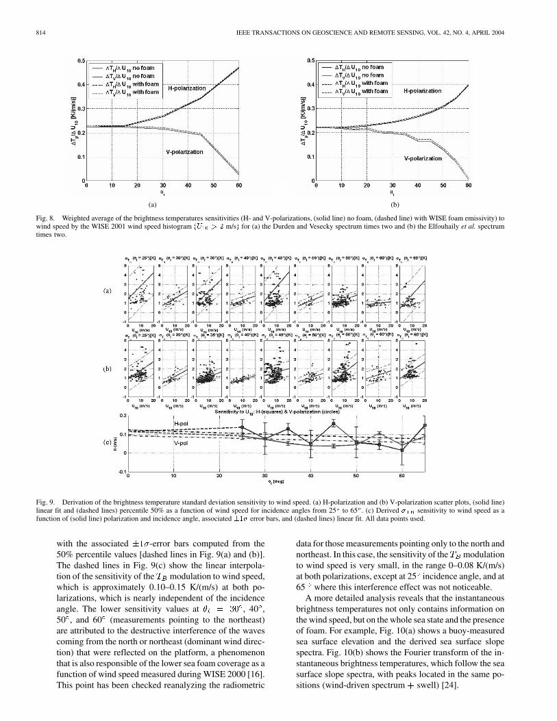
814 IEEE TRANSACTIONS ON GEOSCIENCE AND REMOTE SENSING, VOL. 42, NO. 4, APRIL 2004
(a) (b)
Fig. 8. Weighted average of the brightness temperatures sensitivities (H- and V-polarizations, (solid line) no foam, (dashed line) with WISE foam emissivity) towind speed by the WISE 2001 wind speed histogram (U > 2 m/s) for (a) the Durden and Vesecky spectrum times two and (b) the Elfouhaily et al. spectrumtimes two.
Fig. 9. Derivation of the brightness temperature standard deviation sensitivity to wind speed. (a) H-polarization and (b) V-polarization scatter plots, (solid line)linear fit and (dashed lines) percentile 50% as a function of wind speed for incidence angles from 25 to 65 . (c) Derived � sensitivity to wind speed as afunction of (solid line) polarization and incidence angle, associated �1� error bars, and (dashed lines) linear fit. All data points used.
with the associated -error bars computed from the50% percentile values [dashed lines in Fig. 9(a) and (b)].The dashed lines in Fig. 9(c) show the linear interpola-tion of the sensitivity of the modulation to wind speed,which is approximately 0.10–0.15 K/(m/s) at both po-larizations, which is nearly independent of the incidenceangle. The lower sensitivity values at , 40 ,50 , and 60 (measurements pointing to the northeast)are attributed to the destructive interference of the wavescoming from the north or northeast (dominant wind direc-tion) that were reflected on the platform, a phenomenonthat is also responsible of the lower sea foam coverage as afunction of wind speed measured during WISE 2000 [16].This point has been checked reanalyzing the radiometric
data for those measurements pointing only to the north andnortheast. In this case, the sensitivity of the modulationto wind speed is very small, in the range 0–0.08 K/(m/s)at both polarizations, except at 25 incidence angle, and at65 where this interference effect was not noticeable.
A more detailed analysis reveals that the instantaneousbrightness temperatures not only contains information onthe wind speed, but on the whole sea state and the presenceof foam. For example, Fig. 10(a) shows a buoy-measuredsea surface elevation and the derived sea surface slopespectra. Fig. 10(b) shows the Fourier transform of the in-stantaneous brightness temperatures, which follow the seasurface slope spectra, with peaks located in the same po-sitions (wind-driven spectrum swell) [24].

CAMPS et al.: WISE 2000 AND 2001 FIELD EXPERIMENTS 815
(a) (b)
Fig. 10. (a) (Solid line) Sample sea surface slope spectrum derived from (dashed line) Waverider buoy-measured sea surface height spectrum, and (b) corre-sponding instantaneous brightness temperature power spectra [(solid line curve) V-polarization and (dashed line) H-polarization]. Brightness temperature spectraderived from Fourier transformation of the instantaneous brightness temperature samples and transformation of frequencies to wave numbers using the deep-watersdispersion relationship.
Fig. 11. Brightness temperature increase versus incidence angle and polariza-tion for a 100% foam-covered sea surface [24].
A correlation has also been found between the peaksin and the instantaneous foam coverage time se-ries. It is estimated that, as compared to a foam-free seaspot, the presence of a 100% foam-covered spot will pro-duce a brightness temperature increase from 10–15 K atV-polarization, and nearly constant and about 6 K at H-po-larization, in the whole range of incidence angles from25 to 65 (see Fig. 11 and [24]). These values, togetherwith the fractional foam coverage estimated as a func-tion of wind speed can be used to estimate the global im-pact on the brightness temperatures. However, it shouldbe noted that this relationship depends on many other pa-rameters rather than wind speed [24]–[26], such as the at-mospheric instability, the salinity, the fetch, etc., and the
variations for the same wind speed value can be signifi-cant. During WISE 2000 and 2001, approximately 20 000and 63 000 different photograms were analyzed. The frac-tional surface foam coverage (all types of foam included)was found to beand , respectively.Note that the wind exponent is approximately the samein both field experiments ( 3.5). Howerver, its impactof the brightness temperatures issmall, and only above 15 m/s is it larger than K.
• Brightness temperature sensitivity to the significant waveheight: To derive the brightness temperature sensitivity tothe significant wave height 6 (SWH), a brightness temper-ature deviation from the flat surface model is computedfrom
SST SSS SWH SST, SSS
SWH (8)
where SST SSS is defined in (2) and cor-responds to the emissivity computed from the Fresnel fieldreflection coefficient at -polarization. Fig. 12 shows theplots of the brightness temperatures deviation due to thesignificant wave height at horizontal (upperrow) and vertical (central row) polarizations versus theSWH, for incidence angles from 25 to 65 , in 5 steps.The solid line in each plot represents the regression lineand the dashed ones the 50% percentile ones. The plotat the lower part of Fig. 12 shows the slope of each re-gression line as a function of the incidence angle, whichcorresponds to the average sensitivity to SWH in Kelvinsper meter at H- and V-polarizations. A linear fit of these
6Significant wave height as used in (8) is the average of the highest third ofthe waves.

816 IEEE TRANSACTIONS ON GEOSCIENCE AND REMOTE SENSING, VOL. 42, NO. 4, APRIL 2004
Fig. 12. Derivation of the brightness temperature sensitivity to SWH (a) �T and (b) �T scatter plots, (solid line) linear fit and (dashed lines)percentile 50% as a function of the SWH for incidence angles from 25 to 65 . (c) Derived SWH sensitivity as a function of (solid line) polarization and incidenceangle associated �1� error bars, and (dashed lines) linear fit.
values leads to the following relationships and correlationcoefficients:
SWH
SWH (9)
The extrapolated sensitivity at nadir is then
K/m (10)
Equation (9) has also successfully been used in sea surfacesalinity retrieval algorithms and has proved to be morerobust than (4), when satellite-derived wind speed is used[27] (Section IV).
• Brightness temperature azimuthal angle signature: Wemust distinguish two different regimes: low to moderateand strong wind conditions. The first one was dominantduring all WISE 2000 and part of WISE 2001. In thisregime, the azimuthal signature is very weak—almostinexistent—and difficult to identify. In the strong-windconditions that happened during the first half of November2001, the brightness temperature azimuthal signature isquite clear, reaching a few Kelvin.
Camps et al. [16, Fig. 11] shows typical measurements(5-min averaging) of azimuth scans at horizontal (left) andvertical (right) polarizations for three different low to moderatewind speeds and incidence angles: (a) and (b) ,
m/s, (c) and (d) , m/s, and(e) and (f) , m/s. Even though there arevery few data points covering about one third of a full 360scan, a small 0.1–0.2 K difference is suspected. At L-band,
TABLE IIICOMPUTED T =T PEAK-TO-PEAK AZIMUTHAL MODULATION OF THE
BRIGHTNESS TEMPERATURE FOR DIFFERENT WIND SPEEDS USING
THE SSA METHOD AND ELFOUHAILY et al.’s SEA SPECTRUM.OTHER PARAMETERS: SSS = 38 psu, SST = 20 C
the azimuthal signature computed with two-scale methodsstrongly depends on the spectrum spreading function [5], [20].Table III summarizes the peak-to-peak variations at differentwind speeds and incidence angles computed with the SSAmethod and Elfouhaily et al.’s sea spectrum.
On November 10 and 15, 2001, the two strongest stormswere recorded on the platform. Meteorological and oceano-graphic conditions were similar in both storms, except for thewind direction: northwest on November 10 and northeast onNovember 15. Only measurements corresponding to November10 are available, since the radiometer control was lost onNovember 15, around 11 A.M.
Fig. 13(a) shows a time series of consecutive measurements(one sample per second) at vertical and horizontal polarizationsfor various azimuth angles at 45 incidence angle, while thestorm was becoming more and more intense. Average windspeed at 10 m is just 11.0 m/s, but the significant wave heightcorresponds to the highest peak in Fig. 5. The large standarddeviation of the measurements—several Kelvin—is due to thebrightness temperature modulation produced by the waves [24],and the highest brightness temperature peaks correspond to wave

CAMPS et al.: WISE 2000 AND 2001 FIELD EXPERIMENTS 817
(a) (c)
(b) (d)
Fig. 13. (a) Series of samples acquired during an azimuth scan at 45 incidence angle. November 10, 2001, 19 h. U = 11:0 m/s, (b) Average values andaverage values plus minus one standard deviation for each azimuth angle (with respect to the north) corresponding to (a). (c) Series of samples acquired during anazimuth scan at 55 incidence angle. November 10, 2001, 20 h, U = 12:4 m/s. (d) Average values and average values plus minus one standard deviation foreach azimuth angle corresponding to Fig. 13(c).
breaking events, when foam is produced. Note also the correla-tion between the values averaged at each azimuth angle and theazimuth angle. The linear trend observed on is probably dueto the fact that the storm was becoming more and more intense.Fig. 13(b) shows the average value (crosses) and the averagevalue plus minus one standard deviation (triangles) of the valuesshown in Fig. 13(a), plotted versus the azimuth angle with respectto the south. Fig. 13(c) and (d) shows another azimuth scan at55 incidence angle. As in the former case, the and signalshave a standard deviation larger than instruments radiometricsensitivity, but the average values are correlated to the azimuthangle. As can be appreciated in Fig. 13(d), the amplitude of theazimuthal signal is smaller in than in the former case, since thesensitivity to wind speed vanishes around 55 incidence angle.
It should be pointed out that the measured amplitude modula-tions are too large as compared to model predictions (Table III),even if Elfouhaily et al.’s sea spectrum were multiplied by two.Further research is needed to understand its origin, peakierwaves due to nonfully developed sea, wave foam emission andasymmetric foam distribution, etc.
IV. APPLICATION TO MULTIANGULAR SEA
SURFACE SALINITY RETRIEVAL
The empirical models developed in the Section III are nowapplied to the performance study of sea surface salinity retrievalalgorithms, including the impact of errors in the ancillary data(wind speed and sea surface temperature). The algorithm usedhere to retrieve the salinity from brightness temperature data isa recurrent least squares fit called Levenberg–Marquardt [28]. Ithas been chosen for its easy implementation and computationalefficiency. The brightness temperatures are computed setting aninitial guess for sea salinity, temperature, and wind speed (orsignificant wave height) into the direct emissivity model [(1)and (9)] using the Klein and Swift’s dielectric constant model[13]. This value is compared with the brightness temperaturesmeasured by the radiometer, and then an increment SSS isadded to the initial salinity. An increment can also be addedto the wind speed, which is found to be a critical parameter.It happens that the actual wind speed is not representative ofthe actual sea state, and an “effective” wind speed can be found

818 IEEE TRANSACTIONS ON GEOSCIENCE AND REMOTE SENSING, VOL. 42, NO. 4, APRIL 2004
Fig. 14. SSS retrieval errors as function of the number of measurements(incidence angles + polarizations).
by the SSS retrieval algorithm that best fits the measurements.This recursive method is stopped when the difference betweenthe measured and the computed is smaller than a specifiedthreshold. Fig. 14 shows the retrieval error in 25 different caseswhen using different number of available measurements (inci-dence angles and polarizations). It is, however, surprising thefast decrease of SSS with the number of available measure-ments. Wind speed and sea surface temperature data have beentaken from buoy measurements. Only scans with 12 or moredata points (different incidence angles and polarizations) havebeen used. It is clear that the SSS retrieval quality increases withthe number of measurements.
In the SMOS case, the salinity retrieval problem requiresthe knowledge of other variables (wind speed or significantwave height and sea surface temperature) as close as possibleboth in time and space to the radiometric measurements. Errorsin these parameters translate into sea surface salinity errors.During WISE field experiments, QUIKSCAT and AVHRRsatellite measurements were acquired, as well as data from theARPEGE numerical weather model.
QUIKSCAT Wind speed data: In this study, wind speedproducts of the NASA satellite-borne QUIKSCAT scat-terometer with 2-m/s accuracy and 25-km spatial reso-lution were used. They are colocated with the platformusing a radius of 0.27 latitude and 0.37 longitude. DuringWISE 2000 and 2001, 196 and 74 datasets were available,respectively. Since the scatterometer cannot measure closerthan 50 km from the coast, there were no measurementscoincident with the platform: they were mostly southeast,the closest 3 km away from the platform, the farther 40 kmaway. These wind speed data were averaged for each satel-lite pass, and the resulting averages were compared with1-h average of the in situ measurements. During WISE2000, when compared to the oil rig meteorological sta-tion measurements brought at 10-m height in neutral at-mosphere, the average difference is 0.44 m/s, with 2.8-m/sstandard deviation of the difference. During WISE 2001,there were not enough data to make the comparison with areasonable statistical significance.
AVHRR SST data: LAC images of the AVHRR instru-ment at a spatial resolution of 1.1 km were recordedand processed by the Service d’Archivage et de Traite-ment Meteorologique des Observations Spatiales,Méteo-France/CNRS (SATMOS) data center. Manyimages were cloudy. AVHRR SST estimates have anuncertainty up to 0.1 C in clear sky conditions, and0.3 C otherwise. During WISE 2000, the Ebro fresh andusually colder plume was observed and even reached theCasablanca oil rig, but not during WISE 2001.ARPEGE wind speed data: Surface wind speeds fromthe analyzed surface fields of ARPEGE, Méteo-France’smeteorological model, have been colocated with theCasablanca Platform. The resolution of the model is 25km, 6 h, and the uncertainty is 2.15 m/s. The colocationradius is the same as for QUIKSCAT, i.e., 0.27 latitudeand 0.37 longitude, resulting in nine grid points colocatedfor each field. The data are from October 1 to November30, 2001.
Fig. 15(a) shows the errors on the retrieved salinity for fourdifferent sources of wind speed: 1) wind measured in situ bythe buoy anemometer ( SSS psu, psu);2) wind from QUIKSCAT satellite ( SSS psu,
psu);7 3) wind from ARPEGE model( SSS psu, psu); and 4) leaving thewind as an unknown parameter within the range of the mea-sured value plus or minus the measurement error, and allowingthe retrieval algorithm to derive the values of salinity and an“effective” wind speed ( SSS psu, psu;and WS m/s, m/s).
It can be appreciated that when the measured wind haslarge errors, the retrieved salinity values also have large errors
2 psu . In this case, the option of leaving the wind as afree parameter seems to improve significantly the retrievedsalinity as compared to case of having the wind speed valuefixed. Fig. 15(b) shows the retrieved salinity error and error barwhen using the buoy-measured SST plus 0.3 C random errorto simulate AVHRR-derived SST.8 As expected from the lowsensitivity to sea surface temperature, in these cases there is nosignificant difference among them.
Finally, Fig. 16 plots the retrieved salinity error as a func-tion of the wind speed and the significant wave height. It canbe appreciated that the salinity retrieval error increases withboth wind speed and significant wave height. This effect is notfully understood, but may be probably due to limited fetch andfoam effects not directly included in the models.9 Since thefoam coverage increases with wind speed, and it increases thebrightness temperature, the retrieval algorithm tends to decreasethe retrieved salinity to compensate for the brightness tempera-ture increment. The same happens when considering the signif-icant wave height, which is strongly correlated to wind speed,except in a few situations of swell. Then mean salinity error
7In datasets 10–12, QuikSCAT wind speed is much higher than the one ob-served by the buoys.
8Most days were cloudy, and AVHRR SST was not available.9Note that in the derivation of (1) and (9), the larger number of data points
corresponds to wind speeds smaller than 10 m/s, where the foam fraction cov-erage is negligible.

CAMPS et al.: WISE 2000 AND 2001 FIELD EXPERIMENTS 819
(a) (b)
Fig. 15. Sea surface salinity retrieval error (absolute value) using (a) four different sources of wind speed: measured by the buoy, measured by QUIKSCAT,ARPEGE model, and left as a free parameter (with constraints) in the retrieval algorithm and (b) buoy-measured STT plus 0.3 C random error to simulatedAVHRR-derived SST.
(a)
(b)
Fig. 16. Sea surface salinity retrieval error dependence with (a) wind speed and (b) significant wave height.
and standard deviation when using wind speed and significantwave height are SSS psu, psu, and
SSS psu, psu, respectively. Despitethe worse results of using the significant wave height informa-tion, further analyses are required to determine its potential ad-vantage, since the significant wave height dependence is lessvariable than the wind speed, and that it includes other surfaceroughness effects not due to local winds.
V. CONCLUSION
The results of the L-band radiometric data acquisition andprocessing of WISE 2000 and 2001 field experiments have beenpresented. During WISE 2000, much data were corrupted by
RFI, and derived brightness temperatures sensitivities to windspeed were in agreement with previous [1] measurements, butthe associated error bounds were large. In WISE 2001, the sit-uation improved dramatically, mainly because the 2000 drillingactivities in the platform had already finished. The processingof the data reveals the following.
• A sensitivity to wind speed extrapolated at nadir of0.23 K/(m/s), or a little bit higher 0.25 K/(m/s)
when the atmospheric instability or only the measure-ments corresponding to m/s are accountedfor. This sensitivity increases at H-polarization up to
0.5 K/(m/s) at 65 , and decreases at V-polarizationdown to 0.2 K/(m/s) at 65 , with a zero-crossingaround 55 to 60 . These results are in agreement

820 IEEE TRANSACTIONS ON GEOSCIENCE AND REMOTE SENSING, VOL. 42, NO. 4, APRIL 2004
with the SSA method using Durden and Vesecky’s andElfouhaily et al.’s sea spectra times two. It is very likelythat the computed wind speed sensitivities below 2 m/sare erroneous.
• A modulation of the instantaneous brightness tempera-tures due to wave slopes (and also foam), which makes thestandard deviation of this modulation increase with windspeed at a rate of 0.1–0.15 K/(m/s), depending on polar-ization, and very weakly on incidence angle.
• A sensitivity to significant wave height extrapolated tonadir of 1 K/m, increasing at H-polarization up to1.5 K/m at 65 , and decreasing at V-polarization down to
0.5 K/m at 65 .• A small azimuthal modulation 0.2–0.3 K for low to mod-
erate wind speeds, in reasonable agreement with numer-ical models. However, a large peak-to-peak modulation of4–5 K was measured during a strong storm recorded onNovember 10, 2001.
The brightness temperature sensitivity to wind speed and sig-nificant wave height has been obtained and compared satisfacto-rily to numerical models. Multiangular brightness temperaturedata has been successfully used to retrieve sea surface salinitywith a 0.52-psu bias and 0.12-psu rms error using the derivedwind speed sensitivities. This work is a step forward to the de-velopment of operational sea salinity retrieval algorithms fromspace for the SMOS mission.
ACKNOWLEDGMENT
The WISE 2000 and 2001 field experiments were sponsoredby ESA. The French moorings were supported by the CNES,and the buoy data handling by Méteo-France, with specialthanks to P. Blouch. The radiometric data processing, fieldexperiment logistics, and salinity retrieval studies were spon-sored by the Spanish grants MCYT TIC 2002-04451-C02-01and PNE 009/2001-C-02. Last, but not least, the authors verymuch appreciate all the cooperation and help provided bythe personnel of Repsol Investigaciones Petrolíferas—BaseTarragona—Plataforma Casablanca for the organization ofthe field experiment, without whose help WISE could nothave been performed. The authors are very grateful to fouranonymous reviewers whose detailed and careful review hashelped to increase the clarity of this work.
REFERENCES
[1] C. T. Swift and R. E. McIntosh, “Considerations fro microwave remotesensing of ocena-surface salinity,” IEEE Trans. Geosci. Electron., vol.GE-21, no. 4, pp. 480–491, Oct. 1983.
[2] P. Silvestrin, M. Berger, Y. Kerr, and J. Font, “ESA’s second Earth Ex-plorer Opportunity Mission: The Soil Moisture and Ocean Salinity mis-sion—SMOS,” IEEE Geosci. Remote Sensing Newslett., no. 118, pp.11–14, Mar. 2001.
[3] M. Martín-Neira and J. M. Goutoule, “A two-dimensional aperture-syn-thesis radiometer for soil moisture and ocean salinity observations,” ESABull., no. 92, pp. 95–104, Nov. 1997.
[4] G. S. E. Lagerloef, “Report of the 3rd Workshop, SalinitySea Ice Working Group,” Earth and Space Res., Seattle, WA,http://www.esr.org/ssiwg3/SSIWG_3.html, 2000.
[5] J. Johannessen et al., “Scientific requirements and impact of space ob-servations of ocean salinity for modeling and climate studies,”, ESAcontract 14 273/00/NL/DC, 2002.
[6] A. Camps, J. Font, J. Etcheto, V. Caselles, and A. Weill, “WISE 2000and 2001: Campaign description and executive summary,” in Proc. Eu-roSTARSS, WISE, LOSAC Workshop, 2003, ESA SP-525, pp. 17–26.
[7] R. Villarino, L. Enrique, A. Camps, I. Corbella, and S. Blanch, “Design,implementation and test of the UPC L-band automatic radiometer,” inProc. URSI Commission-F 2002 Open Symp., Garmisch-Partenkirchen,Germany, Feb. 2002.
[8] W. Reich, “A radio continuum survey of the northern sky at 1420MHz—Part I,” Astron. Astrophys. Suppl. Ser., vol. 48, pp. 219–297,1982.
[9] P. Reich and W. Reich, “A radio continuum survey of the northern skyat 1420 MHZ—Part II,” Astron. Astrophys. Suppl. Ser., vol. 63, pp.205–292, 1986.
[10] H. J. Liebe, “MPM—An atmospheric millimeter wave propagationmodel,” Int. J. Inf. Millim. Waves, vol. 10, no. 6, pp. 631–650, 1989.
[11] A. Camps, F. Torres, I. Corbella, J. Bará, and X. Soler, “Calibration andexperimental results of a two-dimensional interferometric radiometerlaboratory prototype,” Radio Sci., vol. 32, no. 5, pp. 1821–1832,Sept.–Oct. 1997.
[12] A. Camps, I. Corbella, M. Vall-llossera, N. Duffo, F. Torres, R. Villarino,L. Enrique, J. Miranda, F. Julbé, J. Font, A. Julià, C. Gabarro’, J. Etch-etto, J. Boutin, A. Weill, V. Caselles, E. Rubio, P. Wursteisen, M. Berger,and M. Martín-Neira, “L-band sea surface emissivity: Preliminary re-sults of the WISE-2000 campaign and its application to salinity retrievalin the SMOS mission,” Radio Sci., vol. 38, no. 4, p. 8071.
[13] L. A. Kelin and C. T. Swift, “An improved model for the dielectric con-stant of sea water at microwave frequencies,” IEEE J. Oceanic Eng., vol.OE-2, no. 1, pp. 104–111, 1977.
[14] W. Ellison, A. Balana, G. Delbos, K. Lamkaouchi, L. Eymard, C.Guillou, and C. Prigent, “New permittivity measurements of sea water,”Radio Sci., vol. 33, no. 3, pp. 639–648, May–June 1998.
[15] S. Blanch and A. Aguasca, “Sea water dielectric permittivity models:Review and impact on the brightness temperature at L-band,” inProc. EuroSTARSS, WISE, LOSAC Workshop, 2003, ESA SP-525, pp.137–142.
[16] A. Camps, J. Font, J. Etcheto, V. Caselles, A. Weill, I. Corbella, M.Vall-llossera, N. Duffo, F. Torres, R. Villarino, L. Enrique, A. Julià, C.Gabarró, J. Boutin, E. Rubio, S. C. Reising, P. Wursteisen, M. Berger,and M. Martín-Neira, “Sea surface emissivity observations at L-band:First results of the wind and salinity experiment WISE 2000,” IEEETrans. Geosci. Remote Sensing, vol. 40, pp. 2117–2130, Oct. 2002.
[17] J. P. Hollinger, “Passive microwave measurements of sea surface rough-ness,” IEEE Trans. Geosci. Electron., vol. GE-9, no. 3, pp. 165–169,1971.
[18] C. T. Swift, “Microwave radiometer measurements of the cape codcanal,” Radio Sci., vol. 9, no. 7, pp. 641–653, 1974.
[19] A. Guissard, Atmospheric Instability Above the Ocean and Implicationsfor Scatterometry, Dec. 2001, submitted for publication.
[20] M. Vall-llossera, J. Miranda, A. Camps, and R. Villarino, “Sea surfaceemissivity modeling at L-band: An inter-comparison study,” in Proc. Eu-roSTARSS, WISE, LOSAC Workshop, 2003, ESA SP-525, pp. 143–154.
[21] S. L. Durden and J. F. Vesecky, “A physical radar cross-section modelfor a wind-driven sea with swell,” IEEE J. Oceanic Eng., vol. OE-10,pp. 445–451, 1985.
[22] T. Elfouhaily, B. Chapron, K. Katsaros, and D. Vandermark, “A unifieddirectional spectrum for long and short wind-driven waves,” J. Geophys.Res., vol. 102, pp. 15 781–15 796, 1997.
[23] C. Cox and W. Munk, “Measurements of the roughness of the sea surfacefrom photographs of the sun’s glitter,” J. Opt. Soc. Amer., vol. 44, pp.838–850, 1954.
[24] R. Villarino, A. Camps, M. Vall-llossera, J. Miranda, and J. Arenas, “Seafoam and sea state effects on the instantaneous brightness temperaturesat L-band,” in Proc. EuroSTARSS, WISE, LOSAC Workshop, 2003, ESASP-525, pp. 95–104.
[25] E. Monahan and I. Muircheartaigh, “Whitecaps and the passive remotesensing of the ocean surface,” Int. J. Remote Sens., vol. 7, no. 5, pp.627–642, 1986.
[26] E. Monahan and M. Lu, “Acoustically relevant bubble asemblages andtheir dependence on meteorological parameters,” IEEE J. Oceanic Eng.,vol. 15, Oct. 1990.
[27] C. Gabarró, J. Font, A. Camps, and M. Vall-llossera, “Retrieved seasurface salinity and wind speed from L-band measurements for WISEand EUROSTARRS campaigns,” in Proc. EuroSTARSS, WISE, LOSACWorkshop, 2003, ESA SP-525, pp. 163–172.
[28] W. Press, S. Teukolsky, W. Vetterling, and B. Flannery, NumericalRecipes in C. The Art of Scientific Computing, 2nd ed. Cambridge,U.K.: Cambridge Univ. Press, 1992.

CAMPS et al.: WISE 2000 AND 2001 FIELD EXPERIMENTS 821
Adriano Camps (S’91–A’97–M’00–SM’02) wasborn in Barcelona, Spain, in 1969. He received theTelecommunications Engineering degree and thePh.D. degree in telecommunications engineering in1992 and 1996, respectively, both from the Poly-technic University of Catalonia (UPC), Barcelona,Spain.
From 1991 to 1992, he was with the ENS des Télé-communications de Bretagne, Bretagne, France, withan Erasmus Fellowship. In 1993, he joined the Elec-tromagnetics and Photonics Engineering group, at the
Department of Signal Theory and Communications, UPC, as an Assistant Pro-fessor, and since 1997 as an Associate Professor. In 1999, he was on sabbaticalleave at the Microwave Remote Sensing Laboratory, University of Massachu-setts, Amherst. His research interests are microwave remote sensing, with spe-cial emphasis in microwave radiometry by aperture synthesis techniques. Hehas performed numerous studies within the frame of European Space AgencySMOS Earth Explorer Mission. He is an Associate Editor of Radio Science.
Dr. Camps received the second national award of university studies in1993, the INDRA award of the Spanish Association of TelecommunicationEngineering to the best Ph.D. in 1997, the extraordinary Ph.D. award at theUniversitat Politècnica de Catalunya in 1999, the First Duran Farell Awardand the Ciudad de Barcelona Award, in 2000 and 2001, respectively, both forTechnology Transfer; and in 2002, the Research Distinction of the Generalitatde Catalunya for contributions to microwave passive remote sensing. He wasChair of Cal ’01. He is editor of the IEEE Geoscience and Remote SensingNewsletter and President-Founder of the IEEE Geoscience and Remote SensingSociety Spain Chapter.
Jordi Font received the Licenciado and Ph.D. de-grees in physics from the Universitat de Barcelona,Barcelona, Spain, in 1973 and 1986, respectively.
He is currently a Senior Researcher at the Institutde Ciéncies del Mar (CSIC), Barcelona, Spain,since 1991, and is responsible for the PhysicalOceanography Group since 1987. He is the authorand coauthor of 170 communications to scientificsymposia and 70 published papers. He is Adviser ofseven Ph.D. theses. He is a Principal Investigator forseveral Spanish and European research contracts.
His main research activities are physical oceanography; the study of the marinecirculation in the western Mediterranean from hydrographic, current-meter(vessel mounted, moored, and drifting), and satellite measurements; variabilityand dynamics of the ocean surface layer, and shelf-slope exchange processes;and the use of remote sensing of the oceans in studying the marine circulationand dynamics. He is currently Co-Lead Investigator and responsible for oceansalinity in the European Space Agency SMOS mission.
Dr. Font is a member of several international societies and committees andhas participated in 41 oceanographic campaigns.
Mercè Vall-llossera (M’99) received the Senior Telecommunication Engineerand the Doctor Telecommunication Engineering degrees in 1990 and 1994, re-spectively, both from the Polytechnic University of Catalonia (UPC), Barcelona,Spain.
She has been lecturing and doing research at the Department of Signal Theoryand Communications, UPC from 1990 until 1997 as an Assistant Professor andfrom 1997 until present as an Associate Professor. She spent a sabbatical year inMontreal with the scholarship of the “Programme Québécois de Bourses d’ex-cellence” (1996–1997): “Stages de Formation postdoctorale au Québec pour je-unes diplômés étrangers.” Her research interests include numerical methods inelectromagnetism, microwave radiometry, antenna analysis, and design. Cur-rently, her research is mainly related to the study of numerical methods ap-plied to the sea surface emissivity and their characterization at L-band and theMIRAS/SMOS project.
Dr. Vall-llossera, along with the other member of the radiometry group atUPC, was awarded the “Primer Premio Duran Farell de Investigación Tec-nológica” in 2002, and the “Primer Premio Ciutat de Barcelona d’InvestigacióTecnològica” in 2001.
Carolina Gabarró received the degree of telecom-munications engineering from the PolytechnicalUniversity of Catalonia (UPC), Barcelona, Spain,in 1998. She is currently pursuing the Ph.D. degreein microwave remote sensing at the Institute ofMarine Sciences (Institut de Ciéncies del Mar, ICM),Barcelona, Spain.
In 1999–2000, she joined the European SpaceAgency, ESTEC, Noordwijk, The Netherlands,working in ocean color remote sensing.
Ignasi Corbella (M’99) received the Telecom-munications Engineering and Doctor Engineeringdegrees, both from Universitat Politècnica deCatalunya (UPC), Barcelona, Spain, in 1977 and1983, respectively.
In 1976, he joined the School of Telecommuni-cation Engineering in UPC as a Research Assistantin the Microwave Laboratory, were he workedon passive microwave integrated circuit designand characterization. During 1979, he workedat Thomson-CSF, Paris, France, on microwave
oscillators design. In 1982, he became an Assistant Professor at UPC, anAssociate Professor in 1986, and a Full Professor in 1993. He is currentlyteaching microwaves at the undergraduate level in UPC and has designed andtaught graduate courses on nonlinear microwave circuits. During the schoolyear 1998–1999, he worked at NOAA/Environmental Technology Laboratory,Boulder, CO, as a Guest Researcher, developing methods for radiometercalibration and data analysis. His research work in the Department of SignalTheory and Communications, UPC includes microwave airborne and satelliteradiometry and microwave system design.
Núria Duffo (S’91–M’99) received the Telecom-munication Engineer degree from the PolytechnicUniversity of Catalonia (UPC), Barcelona, Spain,and the Doctor in Telecommunication Engineeringfrom UPC, in 1990 and 1996, respectively.
Since 1997, she has been an Associate Professorat UPC. Her current research interests are numericalmethods in electromagnetics, microwave radiometry,antenna analysis, and design.
Francesc Torres received the Ingeniero and Doctor Ingeniero degrees intelecommunication engineering from the Polytechnic University of Catalonia(UPC), Barcelona, Spain, in 1988 and 1992, respectively
In 1988–1989, he was a Research Assistant in the RF System Division, Euro-pean Space Agency, Noordwijk, The Netherlands, devoted to microwave devicetesting and characterization. In 1989, he joined the Antenna-Microwave-Radargroup, UPC, where he is currently an Associate Professor. His main researchinterests are focused on the design and testing of microwave systems and sub-systems. He is currently engaged in research on interferometric radiometers de-voted to earth observation.
Sebastián Blanch was born in Barcelona, Spain, in 1961. He received the In-geniero and Doctor Ingeniero degrees in telecommunication engineering fromthe Polytechnic University of Catalonia (UPC), Barcelona, Spain, in 1989 and1996, respectively.
In 1989, he joined the Electromagnetic and Photonics Engineering Group ,Signal Theory and Communications Department, UPC. He is currently an As-sociate Professor at UPC. His research interests are antenna near-field measure-ments, antenna diagnostics, and antenna design.
Albert Aguasca, photograph and biography not available at the time ofpublication.

822 IEEE TRANSACTIONS ON GEOSCIENCE AND REMOTE SENSING, VOL. 42, NO. 4, APRIL 2004
Ramón Villarino received the degree of telecommunications engineer from thePolytechnic University of Catalonia (UPC), Barcelona Spain, in 2000. He iscurrently pursuing the Ph.D. degree.
He has participated in the development and construction of an L-band ra-diometer in the two WISE (Wind and Salinity Experiment) field experimentssponsored by ESA from 2000 until 2002, and the FROG 2003 field experimentto determine the emissivity of foam at L-band.
Luis Enrique, photograph and biography not available at the time ofpublication.
Jorge José Miranda was born in Las Palmas deGran Canaria, Canary Islands, Spain, in 1973.He received the Telecommunication TechnicalEngineering degree from Las Palmas de GranCanaria University (ULPGC), Spain, and the SeniorTelecommunication Engineering degree fromthe Polytechnic University of Catalonia (UPC),Barcelona, Spain, in 1996 and 2001, respectively. Heis currently pursuing the Ph.D. degree in telecom-munication engineering from UPC. His Ph.D. thesisis focused on the sea surface emissivity at L-band.
It includes the development of new models for determining the sea surfaceroughness and the comparison and improvement of existing emissivity models.
From 1996 to 1999, he was with the Remote Sensing and Radar Laboratory(EUITT-ULPGC), where collaborated in satellite image processing. In 1999, hejoined the Signal Theory and Communications Department, UPC. Since 2002,he has been an Assistant Professor at the UPC.
Juan José Arenas, photograph and biography not available at the time ofpublication.
Agustí Julià studied physics and received theInd.Eng. degree in 1973.
He is currently an electronics engineer. Since1962, he is devoted to physical, biological, andchemical oceanographic instrumentation devel-opment and maintenance. He has participated innumerous sea field experiments performing hydro-graphic, current-meter (vessel mounted, moored,and drifting) and satellite measurements. He is alsointerested in radio and satellite telemetry.
Jacqueline Etcheto was born in Meknes, Morocco,in 1943. She received the Agregation de Physique de-gree and the Docteur es Sciences Physiques degreefor her thesis in space plasma physics in 1965 and1972, respectively, both from the Ecole Normale Su-perieure de Jeunes Filles, Paris, France.
She became a Full-Time Scientist in Centre Na-tional de la Recherche Scientifique in 1965. She ispresently appointed to Laboratoire d’OceanographieDynamique et de Climatologie, Paris, France, asDirecteur de Recherches. From 1965 to 1987, she has
been working on space plasma physics, focusing on studies of propagation andgeneration of waves in the magnetosphere. She was responsible for relaxationsounders onboard GEOS1 (ESA, 1977), GEOS2 (ESA, 1978), and ISEE1(ESA/NASA, 1977), including instrument definition, provision of hardware,data handling, and scientific use of data. In 1988, she became interested inoceanography, using the synergy between remotely sensed measurements andin situ data to study the air–sea CO2 exchange at large scale. Her researchactivity is multiyear estimation of air–sea CO2 flux at regional scale usingboth satellite (wind speed, SST, ocean color) and in situ (PCO2 and relatedparameters, including launching CARIOCA buoys) data. Since 1999, she isinvolved in the preparation of the SMOS satellite (ESA, 2007) intended atdetermining sea surface salinity using L-band radiometry. She is interested inthe development and validation of sea surface emissivity models at L-band,including validation campaigns. She is coordinating the group of Frenchscientists involved in the ocean part of the SMOS project. She has published77 papers in the open literature.
Vicente Caselles received the B.Sc., M.Sc., and Ph.D. degrees in physics fromthe University of Valencia, Valencia, Spain, in 1979, 1980, and 1983, respec-tively.
He is currently Professor of physics of the earth and Head of the ThermalRemote Sensing Group, University of Valencia, Valencia, Spain. He has an 25years expertise in the physical processes involved in the temperature measure-ment using remote sensing techniques, which has been documented through 20books, 15 doctoral theses, 150 papers in international journals, 60 conferencepapers, and 30 reports. He has collaborated with the European Space Agencyas member of the Advisory Group for the Land-Surface Processes and Inter-actions Mission. He is the Manager of the Spanish Atmosphere and ClimateProgramme.
Dr. Caselles is the Chairman of the Spanish Remote Sensing Society.
Alain Weill received the Ph.D. degree in atmospheric sciences from the Uni-versity of Paris VI, Paris, France, in 1971.
He has been with the Laboratoire de Meteorologie Dynamique du CNRS until1975, CNET until 1991, and then at CETP/IPSL/CNRS Vélizy as a Senior Sci-entist. His research activity is devoted to continental and marine atmosphericboundary layer. His current research field involves particularly micrometeoro-logical processes and related remote sensing instruments development and anal-ysis. In complement to his research activity, he was Deputy Head of Environ-ment programme at CNRS and now president of PRIMEQUAL, the French pro-gram on air quality at the Ministry of the Environment (MEDD). He is authorand coauthor of more than 70 papers in refereed international journals.
Dr. Weill is a member of ASA and was nominated as “outstanding member”of ISARS (International Society for Acoustic Remote Sensing) in 1998.
Jacqueline Boutin received the Ph.D. degree in physical methods in remotesensing from the University Paris VII, Paris, France, in 1990.
She is currently a Research Scientist at Laboratoire d’Océanographie Dy-namique et de Climatologie/CNRS, Paris, since 1992. She has widely studiedthe validity of remotely sensed wind speeds and the ocean/atmosphere exchangeof CO at large scale using both satellite (wind speed, SST, ocean color) and insitu data. Since 1999, she has been involved in the preparation of the Soil Mois-ture and Ocean Salinity (SMOS) mission and has focused on the retrieval ofocean salinity from L-band measurements. She is a Principal Investigator onseveral satellite projects [ENVISAT(ESA); ADEOS2(NASA/NASDA); CoI onSMOS (ESA)].

CAMPS et al.: WISE 2000 AND 2001 FIELD EXPERIMENTS 823
Stéphanie Contardo was born in Paimpol, France, in 1977. She received theB.Sc. degree in physics from the University of Rennes, Rennes, France, in1999, and the M.Sc. degree in remote sensing from the University of Toulouse,Toulouse, France, in 2000.
She is currently a Research Assistant at the LODYC, Paris, where she workson the SMOS project.
Raquel Niclós received the B.Sc. and M.Sc. degrees in physics from the Uni-versity of Valencia, Valencia, Spain, in 2000, and 2002, respectively.
Since then, she is a Research Fellow of the Remote Sensing Unit, Thermo-dynamics Department, University of Valencia. Her current thesis research is fo-cused on sa surface temperature (SST) determination within the SMOS Missionof the European Space Agency. She has taken part in all these unit last projectsand field experiments to determine the surface temperature and develop preciseand reliable surface temperature retrieval methodologies: as in WISE-2000 andWISE-2001 (Wind and Salinity Experiment, SMOS Mission), with a method-ology to obtain a high-accuracy SST; SIFLEX-2002 (Solar Induced and Fluo-rescence Experiment of ESA), measuring the surface temperature over a canopyboreal forest target; and the ENVISAT-AATSR (Advanced Along Track Scan-ning Radiometer) Validation Campaign.
Raúl Rivas is currently pursuing the Ph.D. degree at the University of Valencia,Valencia, Spain.
He is currently a Researcher at the Institute of Hydrology of Plains (Commis-sion of Scientific Researches), Buenos Aires, Argentina. He has experience inthe use of remote sensing in hydrology. He is developing his Ph.D. thesis on theestimation of the evapotranspiration with remote sensing data.
Steven C. Reising (S’93–M’98) received the B.S.and M.S. degrees in electrical engineering fromWashington University, St. Louis, MO, in 1989and 1991, respectively. He received the Ph.D.degree from Stanford University, Stanford, CA, in1998, where his dissertation research focused onlow-frequency remote sensing of lightning and itsenergetic coupling to the ionosphere, producingchemical changes and optical emissions.
Since 1998, he has been an Assistant Professor ofelectrical and computer engineering at the Univer-
sity of Massachusetts, Amherst. His technical interests include microwave/mil-limeterwave remote sensing, particularly of the ocean and atmosphere, as wellas radiometer design and miniaturization using MMIC architectures. During1999 and 2000, he was a Navy-ASEE Summer Faculty Fellow at the NavalResearch Laboratory, Washington, DC, and he currently serves as a member ofthe WindSat Science Team. He is the current Editor and past Associate Editorof the IEEE Geoscience and Remote Sensing Society (GRS-S) Newsletter.
Dr. Reising received the URSI/USNC Best Student Paper Prize at the Na-tional Radio Science Meeting in Boulder, CO, in 1998. In 2000, he won anOffice of Naval Research Young Investigator Award (YIP). He was awardeda Lilly Teaching Fellowship in 2001–2002. He is an ex-officio member of theGRS-S AdCom (without vote). He serves as Chair of the Springfield, MA, JointChapter of the IEEE AP, GRS, ED, MTT, and LEOS societies. He is a Memberof URSI Commissions F, G, and H, and is the Commission F Co-Chair of theInternational URSI Working Group on Solar Power Satellites. He is a memberof the American Meteorological Society, the American Geophysical Union, TauBeta Pi, and Eta Kappa Nu.
P. Wursteisen, photograph and biography not available at the time ofpublication.
Michael Berger received the M.S. degree ingeophysics and the Ph.D. degree in remote sensingfrom the Ludwig-Maximilians University, Munich,Germany, in 1989 and 1996, respectively.
He has been a Scientist with the GermanAerospace Research Establishment (DLR), theGeo-Research Center Potsdam (GFZ), and has beenwith the National Remote Sensing Facility in Harare,Zimbabwe as a long-term expert for the GermanTechnical Cooperation (GTZ). Since 1998, he hasbeen a Project Scientist with the Land Unit of the
Mission Experts Division, European Space Research and Technology Centre(ESTEC), European Space Agency (ESA), Noordwijk, The Netherlands. Hismain responsibility is the scientific definition and preparation of the SoilMoisture and Ocean Salinity (SMOS) mission, ESA’s second Earth ExplorerOpportunity mission, scheduled for launch early 2007.
Manuel Martín-Neira (M’96) received the M.S.and Ph.D. degrees in telecommunication engineeringin 1986 and 1996, respectively, from the Schoolof Telecommunication Engineering, PolytechnicalUniversity of Catalonia, Catalonia, Spain.
From 1989 to 1992, he was was with GMV, aSpanish firm, where he was responsible for severalprojects for the European Space Agency (ESA)related to global positioning satellite navigationwith applications to precise landing and attitudedetermination. Since 1992, with ESA, he has been
in charge of the radiometer activities within the Payload, Equipment, andTechnology Section. During this period, he has been responsible for thetechnology activities related to the Microwave Imaging Radiometer withAperture Synthesis (MIRAS) project.
Dr. Martín-Neira was awarded a Fellowship to work on radiometry at Euro-pean Space Research and Technology Center (ESTEC), Noordwijk, The Nether-lands, in 1988.
Copyright © 2022 FDOKUMEN