Observed variations in convective precipitation fraction and

stratiform area with sea surface temperature

Roberto Rondanelli1,2 and Richard S. Lindzen1

Received 4 March 2008; revised 8 May 2008; accepted 6 June 2008; published 29 August 2008.

[1] This paper focuses on the relation between local sea surface temperature (SST) andconvective precipitation fraction and stratiform rainfall area from radar observations ofprecipitation, using data from the Kwajalein atoll ground-based radar as well as theprecipitation radar on board the TRMM satellite. We find that the fraction of convectiveprecipitation increases with SST at a rate of about 6 to 12%/K and the area of stratiformrainfall normalized by total precipitation decreases with SST at rates between �5 and�28%/K. These relations are observed to hold for different regions over the tropicaloceans and also for different periods of time. Correlations are robust to outliers and toundersampled precipitation regions. Kwajalein results are relatively insensitive to theparameters in the stratiform-convective classification algorithm. Quantitative differencesbetween the results obtained using the two different radars could be explained by thesmoothing in the reflectivity of convective regions due to the relatively large pixel size ofthe TRMM precipitation radar compared to the size of the convective clouds. Although adependence on temperature such as the one documented is consistent with an increase inthe efficiency of convective precipitation (and therefore consistent with one of themechanisms invoked to explain the original Iris effect observations) this is but one step instudying the possibility of a climate feedback. Further work is required to clarify theparticular mechanism involved.

Citation: Rondanelli, R., and R. S. Lindzen (2008), Observed variations in convective precipitation fraction and stratiform area with

sea surface temperature, J. Geophys. Res., 113, D16119, doi:10.1029/2008JD010064.

1. Introduction

[2] The effect of microphysical processes in deep con-vective clouds remains a major source of uncertainty inunderstanding tropical cloud feedbacks on climate. Severalstudies have suggested on the basis of radiative convectiveequilibrium simulations [Sun and Lindzen, 1993; Renno etal., 1994; Emanuel and Pierrehumbert, 1996] and also onobservational grounds [Lindzen et al., 2001; Lau and Wu,2003; Del Genio and Kovari, 2002; Del Genio et al., 2005]that the temperature dependence of microphysical processesin deep convective clouds could result in climate feedbacks.In the context of the model presented by Renno et al. [1994]for instance, a low efficiency of precipitation resulted inwarm and moist climates due to a strong water vaporfeedback. Recently, Clement and Soden [2005] studied thesensitivity of the tropical mean radiative budget in a globalclimate model (GCM) to changes in the circulation andmicrophysics. They found a relatively large sensitivity tochanges in the fraction of cloud that is converted toprecipitation in deep convection compared to changes in

the strength of the Hadley circulation. Also using a GCM,Lau et al. [2005] found that an increased autoconversionrate in the parameterization of warm convective cloudsleads to a stronger hydrological cycle, a reduction in upperlevel cloudiness, and an increase in the overall fraction ofconvective precipitation.[3] Motivated by the previous work, we use radar obser-

vations to study the relation between sea surface tempera-ture (SST) and the fraction of convective precipitation aswell as the stratiform area normalized by precipitation inconvective systems that develop over tropical oceans.Although our motivation for this study arises from theexpectation that precipitation efficiency can control thewater budget in convective systems thus ultimately actingas a climate feedback, we focus exclusively on the obser-vational relation between convective fractions and strati-form area and SST, as opposed to the speculative attributionof a mechanism or the climate implications. We use datafrom the Kwajalein atoll ground-based radar (hereinafterreferred to as KR) and the precipitation radar of the TRMMinstrument (hereinafter referred to as PR), and we relyheavily on the algorithms that classify rainfall pixels intoconvective and stratiform. We realize that besides SST,other properties of the environment in which convectionis growing will have an effect on the water budget of theconvective systems, namely large-scale wind shear, rela-tive humidity of the free troposphere, magnitude of theconvective updrafts, etc. [see, e.g., Ferrier et al., 1996;

JOURNAL OF GEOPHYSICAL RESEARCH, VOL. 113, D16119, doi:10.1029/2008JD010064, 2008ClickHere

for

FullArticle

1Department of Earth, Atmospheric, and Planetary Sciences, Massa-chusetts Institute of Technology, Cambridge, Massachusetts, USA.

2On leave from Department of Geophysics, University of Chile,Santiago, Chile.

Copyright 2008 by the American Geophysical Union.0148-0227/08/2008JD010064$09.00

D16119 1 of 17

Schumacher and Houze, 2006]. All these processes couldprovide plausible mechanisms for the relations betweenSST and detrainment properties documented in the litera-ture. Not only can the local variation of SST be confoundedby other processes that might bias the results but also somemethodological provisions have to be made to account forthe normalization of the results by a measure of convection.These provisions have been frequently overlooked whenanalyzing the climate implications of changes in the area ofdetrainment of convective systems.[4] Notwithstanding these difficulties, there are theoreti-

cal reasons to suppose that a relation between SST and theefficiency of precipitation that is valid for the current andalso for different climates may exist. On the basis of thesetheoretical arguments Lindzen et al. [2001] hypothesizedthat the observed reduction in the normalized area of highcirrus clouds with SST could be primarily associated withan increase in cloud liquid water with SST. As cloud liquidwater increases, the formation of rainfall in convectiveclouds would become more efficient and therefore lesscondensate would be available for detrainment to form thincirrus clouds in the upper troposphere. This is in essence theIris hypothesis. In this paper, we deal, and only indirectly,with one aspect of the hypothesis, namely the possibilitythat an increase in precipitation efficiency with SST man-ifests itself as modifying the partition between the conden-sate that is rained out of the convective regions and thecondensate that is transported to the stratiform anvil. In thisregard, several observational studies, using a combinationof satellite data, have recently provided evidence for anincrease in the efficiency of precipitation with temperatureover the tropical oceans [Del Genio and Kovari, 2002; Lauand Wu, 2003; Del Genio et al., 2005; Lin et al., 2006]. Anincrease in the precipitation efficiency with temperature isof course only one aspect of the problem. Related studieshave dealt with several other aspects of the more generalquestion of whether a negative feedback mediated by thincirrus clouds does indeed exist. Using CERES and MODISdata, Choi and Ho [2006] estimated that about 60% of thetropical cirrus clouds have a positive cloud radiative forcingand therefore variations in their fraction with climate (cur-rently covering �27% of the area of the tropics) couldpotentially induce strong feedbacks. Spencer et al. [2007]found a decrease in the ice tropical clouds during the warmphase of the tropical intraseasonal oscillation associated witha subsequent cooling of the troposphere. Su et al. [2008],however, studied the dependence of high cloud fraction onSST and found only a very small decrease in the cirrus areanormalized by precipitation (similar to the absence of a signaldocumented by Rapp et al. [2005]) and a net positive cloudradiative forcing associated with these clouds. Methodolog-ical limitations related to the choice of the fraction of highcloud, to the choice of the normalization variable used tomeasure the amount of convection, and to the instrumentalsampling in relation to the sampling of the evolution of aconvective system can have a large effect on the quantitativeresults obtained as we will argue in the following sections.Some of these limitations may play a role in the absence ofcorrelation between normalized high cloud and SST found byRapp et al. [2005] and Su et al. [2008].[5] In this paper we focus on the relation between

convective precipitation fraction and stratiform area with

SST over the tropical oceans using two different instrumen-tal data sets. We argue in section 2 that to the extent that thestratiform precipitation region is primarily controlled by thedetrainment of water from the convective regions, thepartition between convective and stratiform precipitationcan be regarded as a useful, although admittedly rough,observable of the water budget in these systems. Section 3presents results using the Kwajalein radar data set. Insection 4 we attempt to extend the analysis to the rest ofthe tropical oceans and we discuss the origin of some of thedifferences found between the two different data sets, inparticular differences in the pixel size, in the stratiform-convective separation algorithm and in sampling. Finally, insection 5 we offer some discussion and conclusions.Appendices A and B deal with the sensitivity of theKwajalein results to the parameters of the stratiform andconvective separation and with the statistical significance ofthe Kwajalein results.

2. Data and Methods

2.1. Stratiform Convective Separation

[6] There are physical as well as observational reasons forseparating the precipitation produced by tropical mesoscaleconvective systems into stratiform and convective. Here wegive a very brief account of these two precipitation typesand the reader is referred to Houze [1993, 1997] for anextensive treatment of the terminology, physics, and obser-vational aspects of the classification. The convective pre-cipitation refers to the regions of the convective system inwhich vertical motion is strong (w > 1 ms�1) and theformation of precipitation occurs mainly through the col-lection of cloud particles (coalescence or riming). On theother hand, stratiform precipitation regions are characterizedby a slow ascent (less than about 1 ms�1) and the growth ofthe precipitation size particles occurs mainly by vapordiffusion on the surface of ice particles that were detrainedfrom the convective region [Rutledge and Houze, 1987;Houze, 1997].[7] From an observational perspective, the weak horizon-

tal gradients of reflectivity in the stratiform regions can bedistinguished from the peakedness of the reflectivity in themost vigorous convective regions, giving the basis for thealgorithms to distinguish between convective and stratiformregions [Steiner et al., 1995]. The two types of precipitationare not independent of each other since the balance of waterin each of the two regions of the system is coupled by thetransport of condensate and water vapor from the convec-tive region to the stratiform region [Houze, 1993]. However,besides detrainment of condensate from the convectiveregions, significant in situ condensation can also occurprovided that there is a source of water vapor in thestratiform region. Observations of mesoscale convectivesystems in the tropics show the existence of a slantwiselayer of ascent originating as a gravity wave response to theconvective heating [Houze, 2004]. This mean ascent in themidtroposphere, with magnitudes of about 0.1 to 1.0 ms�1

[Cotton et al., 1995] provides a supplementary source ofwater vapor to the stratiform region. The relative importanceof each of these two sources of condensate, that is the in situcondensate production and the detrainment from activeconvective regions in observed mesoscale systems, is large-

D16119 RONDANELLI AND LINDZEN: CONVECTIVE PRECIPITATION WITH SST

2 of 17

D16119

ly unknown. However, Gamache and Houze [1983] esti-mated that the transport from the convective updrafts is themost important source of condensate in the stratiform region(about 1.5 to 3 times larger than in situ condensation in thestratiform region). Even if a significant fraction of thecondensate is produced in situ, detrainment from the activeconvective towers seems to be a prerequisite for theexistence of stratiform rainfall.[8] As a consequence of this causal relation between the

condensate produced in the convective elements and thestratiform precipitation, in the early stages of the life cycleof a mesoscale convective system, the precipitation will bemostly convective, whereas in the dissipating stages of thesystem, when detrainment has been efficient in producing acloud anvil and active convective elements have decayed,the precipitation will be mostly stratiform. From theseconsiderations we can expect that the partition betweenstratiform and convective precipitation can change widely ifperiods of time much smaller than the lifetime of the systemare considered. Therefore, in order to assess a possiblechange in the partition of the precipitation between thesetwo categories and SST, there is an essential need for anintegral measure over the life cycle of the system. We define�c as,

�c ¼R t

c tð ÞdtR tc tð Þ þ s tð Þð Þdt

; ð1Þ

where c and s are the total convective and stratiformprecipitation in the mesoscale convective system and t is atimescale sufficiently long to encompass the entire evolu-tion of the system. We also define a measure of the area ofstratiform rainfall to the total precipitation of the system as aproxy for the spatial extent of the detrainment normalizedby a measure of convection,

As ¼R t

as tð ÞdtR tc tð Þ þ s tð Þð Þdt

; ð2Þ

where as(t) is the area of stratiform rainfall at each time overthe life cycle of the system. In estimating the dependence ofthe distributions of �c and As on SST, we ideally would liketo follow a large number of mesoscale convective systemsover their complete life cycle. This would require a hightemporal sampling over an area of a size at least comparableto the size of the largest mesoscale convective systems(a few hundred kilometers).

2.2. Kwajalein Radar

[9] The observational setting described in the previoussection is most nearly found at the Kwajalein ground-basedradar (KR). The KR is located on the Kwajalein atoll in theRepublic of the Marshall Islands (8.7�N, 167.7�E). Theinstrument covers an annular region of 17 km of internalradius and 150 km of external radius, which is enough tocompletely observe most of the mesoscale convectivesystems (about 1% of the systems can have cloud shieldslarger than the area covered by the radar [Houze, 1993]). Thearea covered by the radar is almost completely oceanic. Theradar operates in the S band at a frequency of 2.8 GHz. Inthis work we make use of the University of Washington

Kwajalein data set, in particular the 2A53UWand 2A54UWproducts of the TRMM database, which correspond to thesurface precipitation and the rain type classification, respec-tively. The temporal resolution of the data is about 10 min.We have used the full data set available to date; it comprises49 months between the years 1999 and 2003.[10] The main uncertainties in the estimation of the

average monthly area rainfall measured by the Kwajaleinradar have been identified and quantified by Houze et al.[2004]. All of these uncertainties are also relevant to thestratiform convective separation. The most important un-certainty which accounts for fluctuations of ±30% of themonthly mean value of rainfall is the calibration uncertainty.A calibration of the Kwajalein radar is performed bymatching the areas of radar echo with reflectivity largerthan 17 dBZ at the 6-km level with similar observationsperformed by the precipitation radar on board of theTropical Rainfall Measuring Mission (TRMM) satellite.Other uncertainties include the extrapolation of surfacereflectivity values made from the reflectivity at a higherlevel and the assumed Z-R relationship based on observeddistributions of rain droplet sizes.[11] The classification of echoes into stratiform and

convective is made from reflectivity measurements at thelowest level measured by the radar, following the proceduredeveloped by Churchill and Houze [1984] and furtherrefined by Steiner et al. [1995] and Yuter and Houze [1997].

2.3. SST

[12] We use the Pathfinder Version 5.0 SST data set,which is retrieved using the five channels of the AdvancedVery High Resolution Radiometer (AVHRR). The dailymaps of SST are averaged into 8-day and monthly periods.We use the 8-day period data to construct three time seriesof average SST, one over the region covered by theKwajalein radar and the other two in regions of 5� � 5�and 10� � 10� centered at Kwajalein. Since SST is notestimated over pixels covered by clouds, significant gapscan occur over cloudy periods or regions. We use these tworegions that are larger than the region that is sampled by theradar, in order to increase the accuracy of the average SSTand also to account for the possibility that some detrainingclouds could have originated from convection occurringoutside the Kwajalein radar region.

2.4. Radiosonde Data

[13] Here we use 12-hourly operational soundings atKwajalein (taken at 00Z and 12Z) of temperature and dewpoint from all reported pressure levels for the period 1999–2003. The data were obtained from the NOAA RadiosondeDatabase access Web site (http://raob.fsl.noaa.gov/). Thesoundings were linearly interpolated from the reportedpressure levels to 100 mb intervals from 1000 mb to300 mb and checked for obvious errors (missing data,unphysical values).

3. Kwajalein Radar

3.1. Results

[14] The variables �c and As are calculated for varyingperiods of 8, 16, and 30 days, within the 5 years of availableradar data. Periods in which less than 70% of valid data are

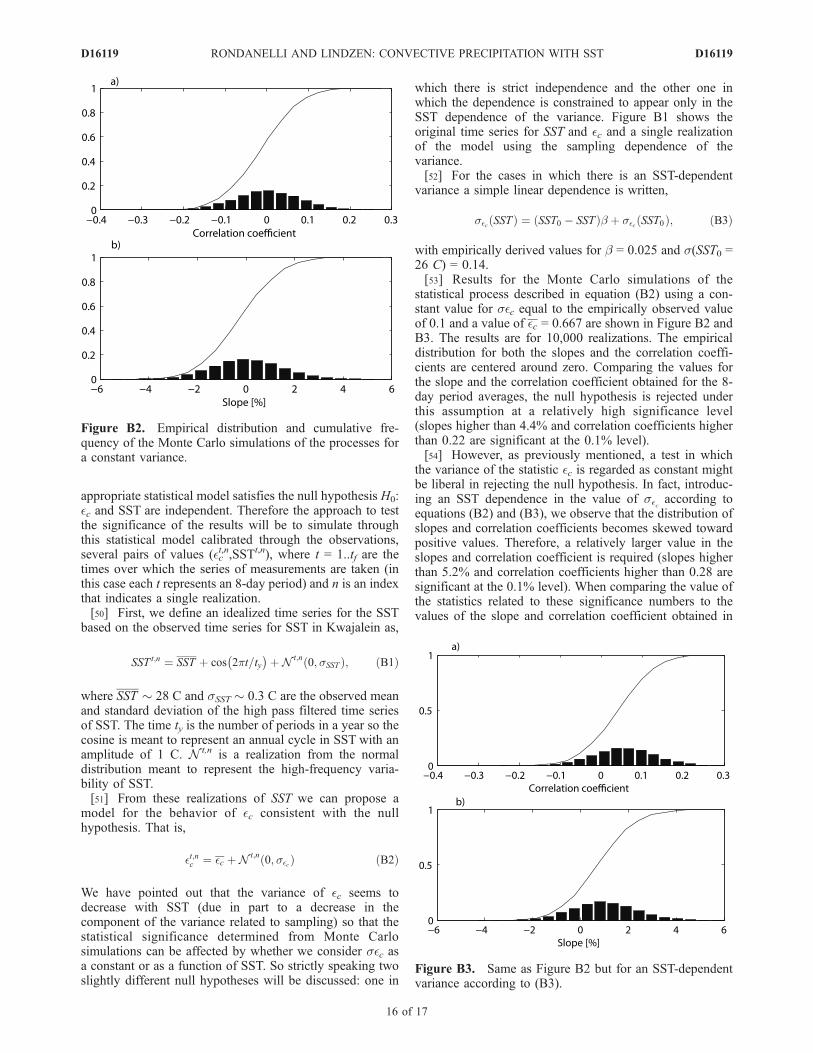
D16119 RONDANELLI AND LINDZEN: CONVECTIVE PRECIPITATION WITH SST

3 of 17

D16119

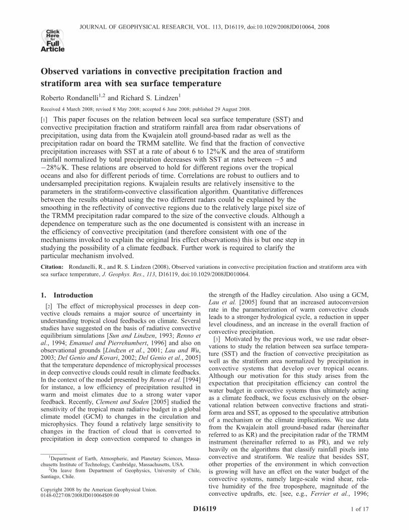
available are discarded from further analysis. Least squareslinear regressions are performed and the slope of the regres-sion (expressed as percentage increase per degree Kelvin) aswell as the correlation coefficient r are shown in Table 1. Thescatter diagram for the period of 8 days using the average SSTover the 10� � 10� is shown in Figure 1.[15] Correlations between �c and SST are positive over the

three different timescales considered and over the differentregions over which the SST is averaged. The values for theslope of the linear regression are between 8%/K and 12%/K.Correlation coefficients are low and explain a relatively smallfraction of the variance of the data (15 to 25%). However, the

scatter is reduced as larger areas and longer periods of timeare considered for the averages. As seen in Figure 1a thevariance of the data seems to decrease with SST. Thebehavior of the variance might be expected given the lowfrequency of rainfall associated with colder SSTs and hencethe temperature dependence of the sampling. We expect alarger scatter at relatively lower rainfall rates and areduction of the difference in variance over the range ofSST as we average over longer periods. This reduction ofthe variance is indeed observed when longer integrationtimes are considered.[16] The normalized stratiform area As has a negative

correlation with SST and the value of the slope rangesbetween �22 and �28%/K. The correlation coefficients areslightly larger than in the case of the correlations between �cand SST. We also notice the relatively large scatter partic-ularly between 27�C and 28�C. When the distribution of theresiduals is calculated some outliers in the correlations areevident (the points that have �c < 0.3 in Figure 1a).Removing these outliers produces an insignificant changein the slopes (from �27.5%/K to �27%/K for As).[17] In order to evaluate the conjecture that the mecha-

nism for the increase in the fraction of convective precip-itation acts through the specific humidity of the airparticipating in convection, we have looked at how corre-lations differ when instead of using SST we use the averagespecific humidity at the surface as measured by the opera-tional soundings at Kwajalein. The rows labeled ‘‘Surfaceq’’ in Table 1 show the results for the linear regression ofspecific humidity q and �c and As. We see that the values ofr are slightly larger than for SST (r is 0.58 for t = 30 daysso they explain up to 35% (r2) of the variance). This is asurprising result given the local nature of the radiosondeobservations compared to the broader spatial extent of theremotely sensed SST. Figures 2a and 2b show the regressionof �c and As against the average q at the surface for a periodof integration of 8 days. In Figure 2c we show a regression

Figure 1. Linear regression between (a) convective fraction �c and (b) stratiform area per unitprecipitation As with respect to the average sea surface temperature (SST) of a region of 10� � 10�around Kwajalein. The period of integration is t = 8 days. The units of As are KR/[mm h�1], where KR isthe area covered by the Kwajalein radar.

Table 1. Percentage Change (%/�K) and Correlation Coefficient

(r) for the Linear Regression Between the Variables �c and As With

Respect to SSTa

�c As

t = 8 t = 16 t = 30 t = 8 t = 16 t = 30

%/�KKR 10.1 8.37 9.37 �24.4 �23.3 �22.5

5� � 5� 11.4 9.3 10.13 �27.0 �25.6 �24.110� � 10� 11.8 10.0 10.21 �27.5 �26.0 �24.4Surface q 9.2 9.0 9.5 �26.3 �25.7 �26.0

rKR 0.39 0.38 0.46 �0.44 �0.48 �0.49

5� � 5� 0.41 0.40 0.47 �0.48 �0.52 �0.5310� � 10� 0.42 0.42 0.48 �0.49 �0.53 �0.53Surface q 0.46 0.49 0.58 �0.53 �0.59 �0.64

aHere t is measured in days. The correlations are for the total of 5 yearsof ground-based radar data and for different periods of integration t of 8,16, and 30 days (the number of observations for the correlations is 162, 76,and 41, respectively, for each of the periods). Only periods in which validdata are available more than 70% of the time are considered. KR (Kwajaleinradar), 5� � 5� and 10� � 10� refer to the areas over which SST data isaveraged, centered at Kwajalein. The row labeled ‘‘surface q’’ shows theresults for the linear regression using the surface q averaged over thecorresponding period instead of SST.

D16119 RONDANELLI AND LINDZEN: CONVECTIVE PRECIPITATION WITH SST

4 of 17

D16119

between the mean SST over the Kwajalein region and thespecific humidity q at the surface. At least two effectscontribute to the scatter. The first is that the measurementsare not completely comparable since the SST is averaged inspace over the entire radar region, whereas q is a localvalue. The second effect and probably the most important isthat the relative humidity is not constant from one period toanother and therefore different values of specific humidityare associated with a single SST. Besides the linear regres-sion, we also plot in Figure 2c the curves corresponding to0.75, 0.80, and 0.85 relative humidity according to theClausius-Clapeyron relationship. We see that most of thedata is contained within the 0.75 and 0.85 curves and thatover the time scale of 8 days only about 40% of the variancein q (r = 0.64) is explained purely by changes in SST.

[18] In Figure 3 we show the result of the regressionbetween �c and specific humidity in the vertical from theradiosonde measurements at Kwajalein. We see that corre-lations (r � 0.4–0.5) and slopes are positive and relativelyconstant up to about 850 mb. The scatter increases above800 mb for all the time scales considered. We see thatmidtropospheric humidity is also positively correlated with�c; however, slopes and scatter are consistently smallerabove the 800 mb level. This is the behavior than onewould expect if the main control of �c would reside in theboundary layer. However, it is also possible that a singlesounding site is less adequate to make inferences in themidtroposphere than in the boundary layer since the vari-ability of specific humidity may be larger (due to episodicevaporative downdrafts and horizontal advection) than in

Figure 2. Linear regression of (a) �c, (b) As and (c) SST averaged over the Kwajalein region on theaverage specific humidity at the surface as measured by the operational soundings at Kwajalein. Theperiod of integration is t = 8 days. (c) Dashed lines show the 0.75, 0.80, and 0.85 relative humiditycurves as calculated from the Clausius-Clapeyron relation for the corresponding SST.

Figure 3. (a) Slope of the regression and (b) correlation coefficient between the convective fraction �cand the specific humidity as measured at different pressure levels by the radiosondes at Kwajalein.Correlations are shown for the three different integration periods.

D16119 RONDANELLI AND LINDZEN: CONVECTIVE PRECIPITATION WITH SST

5 of 17

D16119

the boundary layer where the specific humidity is relativelyclose to 80% of the saturation value at SST.[19] We finally present the regressions using the results

for the period of 8 days in which the sample has beendivided into three similar subsamples according to the totalrainfall observed during the period (Figure 4). The correla-tion coefficients in each of these regressions are smaller(r � 0.2–0.3) than the ones in which the original sample isused, so inferences have to be made with even greatercaution. To the extent that inferences can be made withthese reduced samples, the results suggest that the regres-sions are somewhat dependent on the rainfall amount. Thelargest slopes are found for the lower rainfall category thatcontain some outliers from the original regression. Thismight indicate that some of the original numbers for theslopes of the regression might be overestimated. It mightalso indicate that the linear regression is not adequate in thiscase. For the medium and the higher rainfall categories theslopes appear to be similar, between 4%/K and 6%/K for theincrease of �c and around �10%/K for As (significantlysmaller than the number estimated using the totality of thedata). The fact that at least the two larger rainfall categoriesshow similar regressions might be interpreted as evidencethat midtropospheric humidity variations, that are expected

to be related to the total rainfall over the region, are not adominant factor in the correlations.

4. TRMM Precipitation Radar

[20] Although the KR provides a high temporal andspatial resolution data set of stratiform and convectiverainfall, the data set only represents a very small area ofthe tropical ocean. The obvious choice to extend theanalysis to the rest of the tropical oceans is to use datafrom the precipitation radar on the TRMM satellite (PR).The PR instrument provides estimations for the rainfall andclassification for each rainfall pixel [Awaka et al., 1997;Iguchi et al., 2000; TRMM Precipitation Radar Team, 2005](products 2A23 and 2A25A, version 6). The TRMMsatellite orbits the Earth at a height of about 350 km andwith an inclination of about 35�. The precipitation radar(PR) on board TRMMmeasures at a frequency of 13.8 GHz.Significant attenuation occurs at this frequency primarily byrainfall and has to be corrected before producing theprecipitation product [Iguchi et al., 2000]. The data isgathered over a swath width of 215 km with a horizontalresolution of 4.3 km at nadir (for data before August 2001)and a vertical resolution of 250 m. The instrument is sensitive

Figure 4. Linear regression between (a) �c and (b) As with respect to SST and (c) �c and (d) As withrespect to q at the surface. The colors represent the lower (yellow), medium (blue), and upper (red) tercileof the distribution of rainfall over the period.

D16119 RONDANELLI AND LINDZEN: CONVECTIVE PRECIPITATION WITH SST

6 of 17

D16119

to echoes with reflectivity higher than about 18 dBZ (formore details, see, e.g., Kummerow et al. [1998]).[21] The immediate extension of the Kwajalein analysis

using the PR data is not free of limitations. Perhaps the mostimportant limitation is the inability to resolve mesoscaleconvective systems due to the low temporal resolution ofthe PR orbits. A region of the size of the area covered by theKR will be, on average, completely covered by the footprintof the PR once in about 3 days compared to the 10 min timeresolution provided by the KR. A strategy to use the PRdata has to balance the need to use a sufficiently long periodof time to minimize the sampling error and a sufficientlyshort period of time so that the SST measured over thatperiod is not significantly different from the SST relevant tothe convective timescale.

4.1. Estimating TRMM Sampling Error Using theKwajalein Data Set

[22] In this section we will estimate the sampling errormade by the PR in monthly accumulations of orbital data byusing resampling over the more frequent KR data. We canform synthetic months by taking a piece of the original5 year series long enough so that is larger than thedecorrelation time for the the particular variable observed.In the case of average rainfall, and for this particular grid

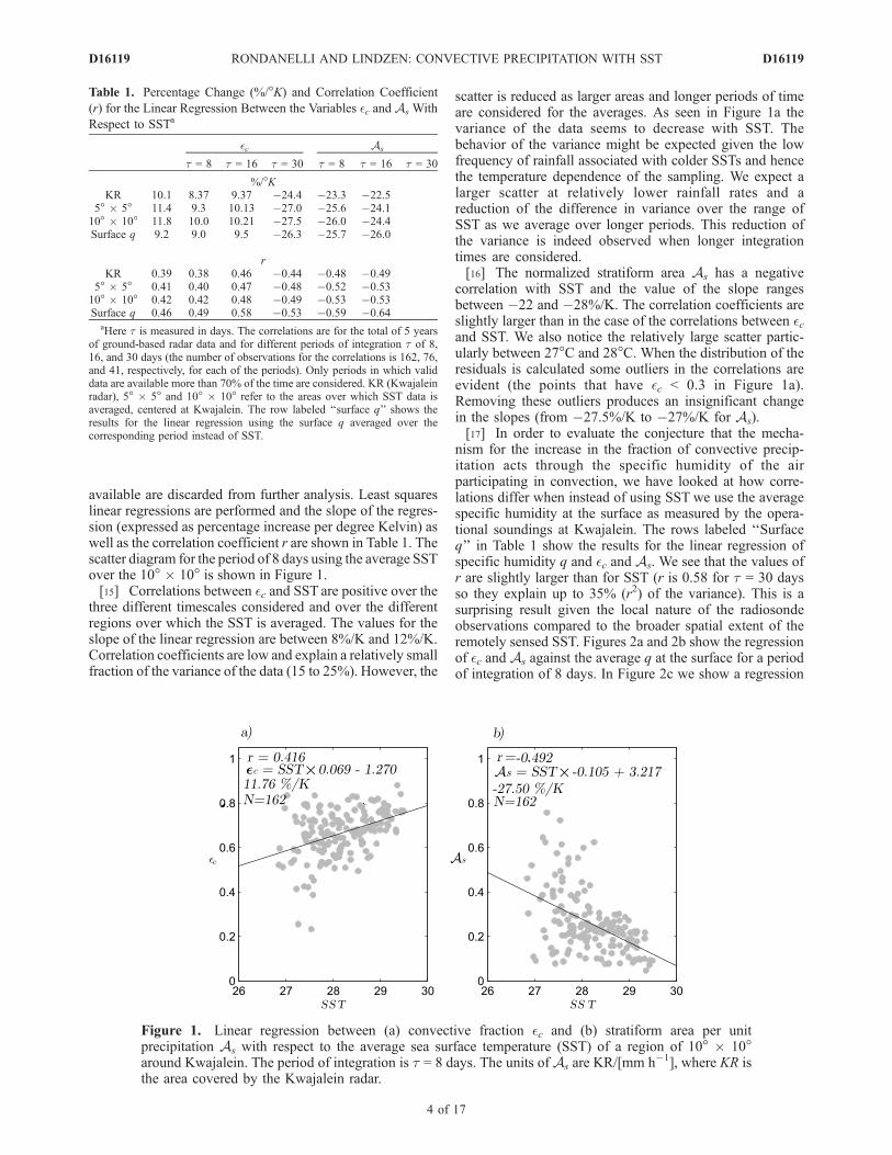
size, the decorrelation time is about 5 days, so we arbitrarilychoose the length to be 10 days. We create 1000 syntheticmonths out of the Kwajalein data and at the same time wepreserve the statistical characteristics of the time series forthe shorter scales. A similar methodology was suggested byBell and Kundu [2000].[23] Figure 5 shows the dependence of the relative root

mean squared error with rainfall for the three variables, �c,As, and R. The curves are least squares fitting of power lawsfor each of the variables. We see that the relative error forrainfall is between 20% and 50% for the revisit time of theTRMM instrument, whereas the sampling error for As isbetween 20% and 30% and the error for �c is only about10%. This behavior seems consistent with the idea of arelatively longer decorrelation timescale for �c and As thanfor R itself as the relative sampling error is inverselyproportional to the decorrelation time. The dependence ofthe sampling error on rainfall is similar to other observa-tional estimates and also to the theoretical model presentedby Bell and Kundu [2000] that predicts a R�1

2 dependence ofthe relative error of rainfall and a sampling error ofmagnitude inversely proportional to the decorrelation time-scale. The power law dependence for the relative samplingerror of rainfall in our case seems to be closer to R�1

5.

Figure 5. Relative sampling error estimated for TRMM revisit times using resampling of the Kwajaleinradar data. The curves are the least squares fitting of a power law for the three variables, �c (dash-dottedline), As (dotted line), and total rainfall R (solid line). The fitting is done for the average value of therelative sampling error binned according to rainfall in mm h�1.

D16119 RONDANELLI AND LINDZEN: CONVECTIVE PRECIPITATION WITH SST

7 of 17

D16119

However a R�12 curve that fits the data is within the standard

deviation of the average of the errors depicted in Figure 5.[24] The existence of the sampling error does not a priori

precludes the possibility of observing a signal in the TRMMdata. The sampling error, if uniform over the range oftemperatures, will only decrease the confidence of theestimation of the parameters of the regression to the extentof the magnitude of the error. Since the scatter of theregression not only depends on the error but also on theproportion of the variance of the error to the variance of thedependent variable, the detection of the signal is madedifficult both by the sampling and also by the relativelysmall range of temperatures over which deep convectionoccurs.

4.2. PR Convective-Stratiform Classification

[25] The classification of echoes among two broad cate-gories is done using both the vertical and horizontalvariability of the reflectivity in TRMM [Awaka et al.,1997; TRMM Precipitation Radar Team, 2005]. Given therelatively high vertical resolution of TRMM of 250 m, abright band (that is, a region of a few hundred meters in thevertical of enhanced reflectivity due to melting of icehydrometeors [Doviak and Zrnic, 1993]) can be determinedproviding a complementary method to the horizontal texture

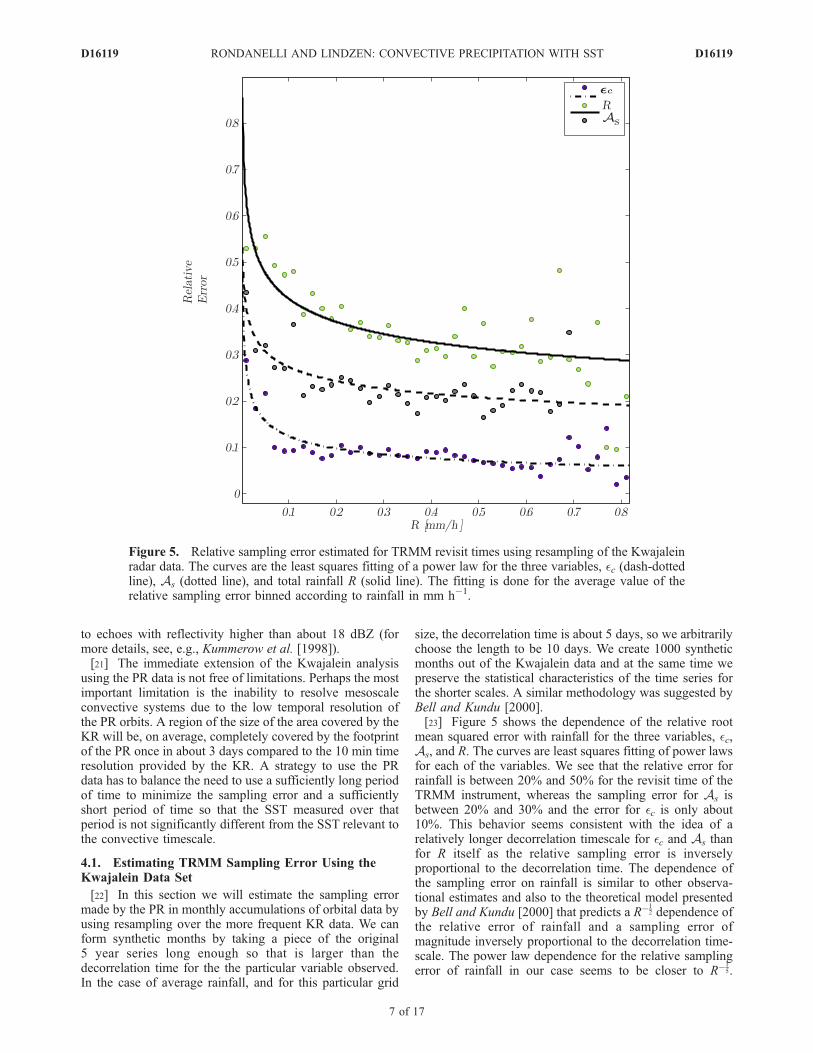
classification algorithms [e.g., Steiner et al., 1995]. Usingthe height of the storm top (the maximum height at whichsignificant echo is observed) a shallow and nonshallowclassification is performed. Also all rainy pixels are classi-fied as isolated or nonisolated, depending on whether theyare surrounded by other rainy pixels.[26] We show in Figure 6 the geographical distribution of

rainfall separated in four broad categories constructed bymerging some of the original categories in the 2A23 productas indicated in Figure 7 for the month of April 2001. We seethat convective and stratiform rainfall pixels are constrainedto the ITCZ regions in the Atlantic and Eastern Pacific(where there is a hint of a double ITCZ) and they are morewidespread in the Indian Ocean and in the Western Pacific.Figure 6d shows the distribution of shallow isolated pixels;these are usually called cumulus congestus and they areprecipitating clouds capped by an inversion layer near thefreezing level as described by Johnson et al. [1999].Although these clouds are convective in nature as arguedby Schumacher and Houze [2003], they are not necessarilyassociated with detraining mesoscale convective systems.Shallow isolated rainfall is more prevalent in subtropical(the Eastern coasts of South America and Australia close to20�S in this particular month), in which no correspondingstratiform or deep convective precipitation is observed.

Figure 6. Rainfall intensity for different categories according to TRMM-PR for April 2001. (a) Seasurface temperature. (b) Convective rainfall (200–240). (c) Stratiform rainfall (100–170). (d) Shallowisolated rainfall (251, 261, 271, 281, 291). (e) Shallow nonisolated rainfall (252, 262, 272, 282).

D16119 RONDANELLI AND LINDZEN: CONVECTIVE PRECIPITATION WITH SST

8 of 17

D16119

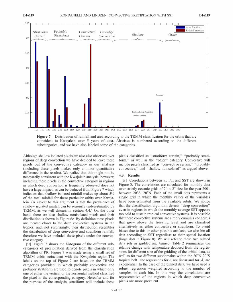
Although shallow isolated pixels are also also observed overregions of deep convection we have decided to leave thesepixels out of the convective category in our analysis(including these pixels makes only a minor quantitativedifference in the results). We realize that this might not benecessarily consistent with the Kwajalein analysis; however,including these pixels in the convective category in regionsin which deep convection is frequently observed does nothave a large impact, as can be deduced from Figure 7 whichindicates that shallow isolated rainfall makes up about 5%of the total rainfall for these particular orbits over Kwaja-lein. (A caveat to this argument is that the prevalence ofshallow isolated rainfall can be seriously underestimated byTRMM, as we will discuss in section 4.4.) On the otherhand, there are also shallow nonisolated pixels and theirdistribution is shown in Figure 6e. By definition these pixelsare located closer to the deep convective systems in thetropics, and, not surprisingly, their distribution resemblesthe distribution of deep convective and stratiform rainfall;therefore we have included these pixels under the convec-tive category.[27] Figure 7 shows the histogram of the different sub-

categories of precipitation derived from the classificationalgorithm of PR. Figure 7 was made using a small set ofTRMM orbits coincident with the Kwajalein region.Thelabels on the top of Figure 7 are based on the TRMMcategories provided, in which probably convective andprobably stratiform are used to denote pixels in which onlyone of either the vertical or the horizontal method classifiedthe pixel in the corresponding category. Hereafter and forthe purpose of the analysis, stratiform will include those

pixels classified as ‘‘stratiform certain,’’ ‘‘probably strati-form,’’ as well as the ‘‘other’’ category. Convective willinclude pixels classified as ‘‘convective certain,’’ ‘‘probablyconvective,’’ and ‘‘shallow nonisolated’’ as argued above.

4.3. Results

[28] Correlations between �c, As, and SST are shown inFigure 8. The correlations are calculated for monthly dataover strictly oceanic grids of 2� � 2� size for the year 2001between 20�S–20�N. Each of the small dots represents asingle grid in which the monthly values of the variableshave been estimated from the available orbits. We noticethat the classification algorithm detects ‘‘deep convection’’even in regions in which the monthly average SST appearstoo cold to sustain tropical convective systems. It is possiblethat these convective systems are simply cumulus congestusthat grow above the freezing level and are classifiedalternatively as either convective or stratiform. To avoidbiases due to this or other possible artifacts, we also bin alldata according to SST regardless to their spatial location(large dots in Figure 8). We will refer to these two relateddata sets as gridded and binned. Table 2 summarizes therelative change with temperature deduced from the regres-sions for different size of the gridding of the orbital data, aswell as for two different subdomains within the 20�N 20�Stropical belt. The regressions for �c are linear and for As areexponential. In the case of the binned data, we have used arobust regression weighted according to the number ofsamples in each bin. In this way the correlations arerepresentative of the regions in which deep convectivepixels are more prevalent.

Figure 7. Distribution of rainfall and area according to the TRMM classification for the orbits that arecoincident to Kwajalein over 5 years of data. Abscissa is numbered according to the differentsubcategories, and we have also labeled some of the categories.

D16119 RONDANELLI AND LINDZEN: CONVECTIVE PRECIPITATION WITH SST

9 of 17

D16119

[29] The gridded data shows a relatively large scatter (r2 isabout 0.25 for both variables). When the regression is takenon the binned data, the scatter and the magnitude of the slopeof the regression are reduced. As shown in section 4.2, thesampling error has a rainfall dependence; on the other hand,rainfall has a positive dependence on temperature over thetropical oceans. Therefore, it is expected only on the basisof the nature of the sampling error that the variance of thegridded data will also show a SST dependence. Consistentwith the sampling error being larger for relatively coldSSTs, the difference between the gridded and binnedregression is largest in the colder regions specially for As

as shown in Figure 8.[30] Table 2 also shows the results for two subdomains;

the Western Pacific (WP) is defined as the region between140�E and 150�W, whereas the EP is the region between150�W and 80�W. Correlations in the EP region have asmaller scatter (for instance, for �c, r

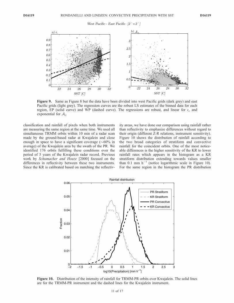
2 = 0.16 in the WPcompared to r2 = 0.28 in the EP) and also a larger slope forthe correlation. Correlations are positive for each regionseparately suggesting that the correlation is universal.Figure 9 shows the regressions for the EP and WP regions.The regression in both figures are the robust regressions forthe binned data sets in each of the regions. In general itseems that for the same SST the EP shows a higher value of�c and a smaller value of As. This seems in apparentcontradiction with observations that indicate a higher pro-portion of stratiform rainfall in the EP than in the WP [e.g.,Berg et al., 2002; Schumacher and Houze, 2003]. However,given the larger proportion of relatively colder SSTs overthe EP, at least for the year 2001 the overall fraction ofconvective precipitation is smaller in the EP than in the WPregion.[31] We notice that �c is smaller for Kwajalein than what

is observed with the PR. However in terms of the relativechange with temperature, PR results seem to agree quanti-

tatively with the range between 8 to 12%/K increase for �cobtained from the Kwajalein observations. In the case of As,PR correlations are smaller than those obtained for KR,specially over the Western Pacific where the relative changein As can be about �5.5%/K, compared to �22%/K forKwajalein. We also notice that the rate of change of As withtemperature seems closer to zero for temperatures higherthan about 28.5 C (Figure 8b), so even an exponentialdecrease does not seem to be an appropriate fit for this partof the curve. This flattening toward higher temperaturesmight be a consequence of the instrument resolution as wewill discuss in section 4.4. However, we can anticipate thatto the extent that PR errors can be reduced by binning thedata with SST, and considering some of the differences inthe instruments as well as in the classification methods, PRand KR seem to agree in the magnitude and sign of thevariation with SST of �c and As.

4.4. Kwajalein and PR Radar Comparison

[32] In order to discuss the differences between theKwajalein and TRMM results, it is useful to compare the

Table 2. Relative Increase in �c and Astr With SST Estimated

From the Regression of the Data From the Precipitation Radar on

Board the TRMM Satellitea

Data Type

2� � 2� 10� � 10�

All WP EP All

�c (%/K) gridded 13.9 13.1 17.8 12.4binned 6.47 6.7 10.7 6.98

As(%/K) gridded �21.8 �15.9 �17.7 �18.9binned �15.6 �5.5 �12.6 �10.2

aThe results are given in (%/�C) at 27�C. ‘‘All’’ refers to the calculationsincluding all oceanic regions. WP and EP stand for western Pacific andeastern Pacific, respectively. All calculations are between 20�S and 20�N,except for the column indicated as 10�S and 10�N.

Figure 8. Regression of the variables (a) �c and (b) As with respect to SST obtained from the TRMMdata set for the year 2001, when the pixel data were aggregated monthly in time and in grids of size 2� �2� in space. Light gray dots are monthly 2� � 2� observations, whereas dark gray circles are obtainedafter adding all data for a given SST range (binned data). The curves in Figures 8a and 8b are differentversions of the least squares fitting (LS) of the data, in linear LS of all the data (dash-dotted line), thelinear LS of all binned data (dashed line), and robust linear LS of the binned data (solid line) in Figure 8a.In Figure 8b the curves are the exponential LS of all data (dash-dotted line), the exponential LS of thebinned data (dashed line), and the robust exponential LS of the binned data (solid line).

D16119 RONDANELLI AND LINDZEN: CONVECTIVE PRECIPITATION WITH SST

10 of 17

D16119

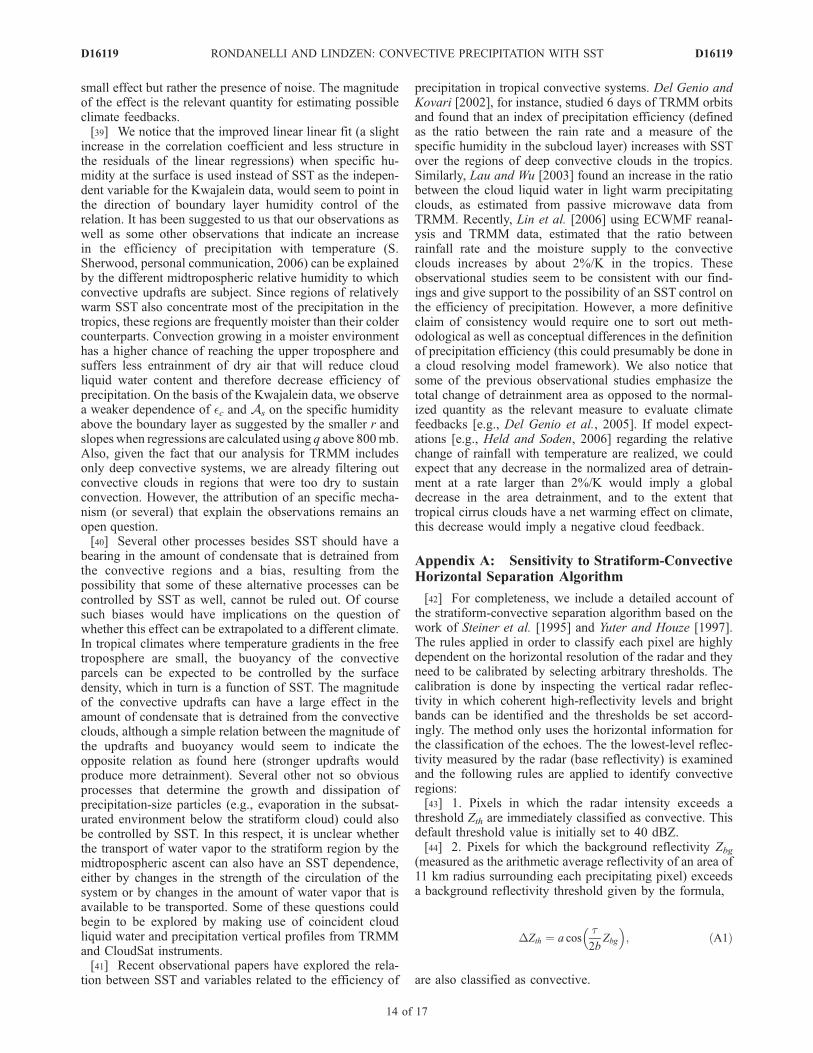
classification and rainfall of pixels when both instrumentsare measuring the same region at the same time. We used allsimultaneous TRMM orbits within 10 min of a radar scanmade by the ground-based radar at Kwajalein and closeenough in space to have a significant coverage (�60% inaverage) of the Kwajalein area by the swath of the PR. Weidentified 176 orbits fulfilling these conditions over theperiod of 5 years of the Kwajalein radar record. Previouswork by Schumacher and Houze [2000] focused on thedifferences in reflectivity between these two instruments.Since the KR is calibrated based on matching the reflectiv-

ity areas, we have done our comparison using rainfall ratherthan reflectivity to emphasize differences without regard totheir origin (different Z-R relations, instrument sensitivity).Figure 10 shows the distribution of rainfall according tothe two broad categories of stratiform and convectiverainfall for the coincident orbits. One of the most notice-able differences is the higher sensitivity of the KR to lowerrainfall rates which appears in the histogram as a KRstratiform distribution extending towards values smallerthan 0.1 mm h�1 (notice logarithmic scale in Figure 10).For the same region in the histogram the PR distribution

Figure 9. Same as Figure 8 but the data have been divided into west Pacific grids (dark grey) and eastPacific grids (light grey). The regression curves are the robust LS estimates of the binned data for eachregion, EP (solid curve) and WP (dashed curve). The regressions are robust, and linear for �c andexponential for As.

Figure 10. Distribution of the intensity of rainfall for TRMM-PR orbits over Kwajalein. The solid linesare for the TRMM-PR instrument and the dashed lines for the Kwajalein instrument.

D16119 RONDANELLI AND LINDZEN: CONVECTIVE PRECIPITATION WITH SST

11 of 17

D16119

begins abruptly at about 0.2 mm h�1 coincident with thelower threshold in reflectivity of the TRMM-PR instrumentof about 17 dBZ. Also, the mode of the convectiveprecipitation distribution is located at a lower rainfall ratefor TRMM probably a consequence of the larger pixel sizein the PR (4.3 km compared to 2 km for KR). For the samereason the KR has a higher frequency of high rainfall ratesthan TRMM.[33] The convective stratiform algorithm is applied to the

reflectivity data before it has been corrected for attenuation,this might result in a misclassification of some convectiveechoes into stratiform. Heymsfield et al. [2000] showcalculations for a bell-shaped reflectivity distributionintended to mimic a single convective cloud. For instanceif we consider a cloud of 1.2 km in diameter (which is themedian diameter of convective updrafts reported over theKwajalein region between 5 and 9 km height [Anderson etal., 2005]) that is centered along the PR beam, the maxi-mum reflectivity is reduced from 50 dBZ to 45 dBZ. For theextreme case in which the convective cloud is located in acorner of the PR footprint, reflectivity is further reduced toless than 10 dBZ, so in this case not only the cloud wouldbe misclassified but it would be undetected by the PR. Boththe misclassification and the nondetection of convectiveclouds due to beam filtering point in the same direction,toward a negative bias in the value of �c and a positive biasof As toward higher convective fractions. Since we havedocumented a convective fraction dependence on SST, thisvery dependence implies a bias with temperature; as ahigher proportion of convective cores are present in thesample there will be a larger amount of those coresmisclassified or missed by the instrument. Rough estimatesusing a 20% of misclassified convective cores and 10%missing cores can explain a 10%/K difference in the valueof the relative change of As. A more precise estimation ofthis effect could be made observationally by comparingTRMM data before and after the satellite’s boost maneuverwhen pixel size increased from 4.3 to 5.0 km (for the smallset of coincident orbits over Kwajalein, the previous numb-ers for the percentage of missing and misclassified coresseems reasonable). From cloud physics considerations, andassuming that correlations are primarily controlled by thespecific humidity of the boundary layer, one could alterna-tively argue that the flattening of the correlations towardhigher temperatures is due to a saturation effect on thechange of the cloud liquid water with temperature ratherthan an instrumental effect. However, the change over theobserved range of temperatures would be too small toexplain the flattening. Additionally, an instrumental effectis favored by the fact that in the higher-resolution data ofKwajalein the flattening is less evident.

4.5. Comparison Between Radar and Infrared CloudAreas

[34] The stratiform rainfall area is one of several observ-ables connected to the detrainment from convective clouds.Lindzen et al. [2001] for instance, used the area of cloudsbetween 220 and 260 K as a proxy for the area ofdetrainment in deep convective regions. Since the area ofprecipitation in a convective system is smaller than the areacovered by clouds, the use of the stratiform rainfall areaminimizes the possibility of an error in which size of the

grid over which the statistics are being taken influences thecorrelations (through the higher rainfall frequency andcoverage of the grids at higher SSTs as discussed by DelGenio and Kovari [2002]). In fact our results do not show astrong dependence on the size of the grids (Table 2). Relatedto this advantage is the fact that precipitation detrained fromthe convective region is short-lived with respect to theclouds, and therefore the error which one incurs by trun-cating the life cycle of the system either in time or in spaceis minimized (in other words, the convective towers inwhich detrainment originates are ‘‘closer’’ in time and spaceto the stratiform rainfall area than to the thin cirrus area).Figure 11 shows the lagged correlation coefficient betweenthe area of stratiform precipitation and the area of the cloudshield over the radar region as measured by the 11 mminfrared satellite brightness temperature. In Figure 11 theinfrared area excludes regions colder than 220 K andincludes regions colder than a certain temperature BT, sowe denote this area by A(BT-220). Lag correlations aremaximized along the solid line in Figure 11 with a lag ofabout 3 h for A(235–220) and a lag of about 10 h forA(275–220). The relatively large values of the correlationcoefficient (�0.6) indicate good correspondence betweenthe rainfall area and the cloud area as measured by theinfrared satellite. Moreover, the increase in the time lag inwhich correlations are maximized for warmer temperaturessuggest that even instantaneous measurements as thosemade by the PR instrument stratiform area capture someinformation on the time evolution of the detrainment(possibly because the sample includes clouds at varioustimes in their evolution).

5. Discussion

[35] We have presented an observational analysis of thedependence of the convective fraction and stratiform area(normalized by total precipitation) on SST. Our motivationfor this analysis, as in other previous work, is to explorewhether we can obtain constraints on observables that arerelated to the water budget of deep convective systems inthe tropics. The declared or undeclared purpose of suchstudies (including ours) is not limited to the characterizationof the natural variability of convective system in the currentclimate, but usually there is the expectation that the currentvariability provided by SST variation in the tropics canserve as a proxy for the changes that can be brought aboutby climate variability on various scales. There are a numberof reasons why a relation between local SST and cloudproperties might exist; however, the present study does notdepend on these assumptions though it occasionally reflectson them. For instance model simulations and theoreticalarguments as well as observations of the present climateindicate that relative humidity remains approximately con-stant with temperature in the tropical boundary layer [e.g.,Held and Soden, 2000]. A simple line of reasoning thatfollows from this indicates that in a warmer climate, thecloud liquid water will increase in a proportion equal to therelative change in the moist adiabatic lapse rate in the lowerpart of the cloud (about 2%/K at 300 K) [e.g., Betts andHarshvardan, 1987], whereas higher up in the cloud, the rateof change will approach the surface Clausius-Clapeyron rateof change (about 6%/K at 300 K, if no precipitation is

D16119 RONDANELLI AND LINDZEN: CONVECTIVE PRECIPITATION WITH SST

12 of 17

D16119

allowed to remove cloud water). Local changes in SSToccurring within the present climate can therefore be likenedto changes that will occur in a different climate as long as theyare uniquely related to changes in specific humidity in thetropical boundary layer. An increase in the liquid watercontent of the clouds will in turn produce an increase in thetime that it takes for precipitation to grow, and simple modelsas well as sophisticated parameterizations of the microphys-ics of clouds have incorporated this behavior.[36] In this paper we focused on the variation with SST of

two observables derived from radar data over the tropicaloceans: �c, the fraction of convective precipitation, and As,the area of stratiform precipitation normalized by totalprecipitation. The normalization is a necessary conditionto obtain a meaningful result since to the first order the SSTdistribution organizes the spatial variation of convection inthe tropics. Cloud properties such as the area of detrain-ment, total rainfall, and cloud radiative effects can beconsidered extensive with respect to the amount of convec-tion. The normalization simply takes into account the factthat the amount of convection in a region of a giventemperature is not indicative of the amount of convectionin a climate with the same temperature, since the globalamount of convection is determined by global energybalance considerations. It remains an open question whethertotal precipitation, mass convective flux, or some othermeasure of convection is the most adequate normalizationfactor with regard to climate effects.[37] Our results show an increase in the fraction of

convective precipitation with SST together with a decreaseof the area of stratiform precipitation per unit of totalrainfall. Results for both instruments indicate an increase

in the fraction of convective precipitation of about 6–12%Kand an decrease in the normalized stratiform area of about5–28%/K. Furthermore, the observations seem to be inde-pendent of the particular geographical area chosen for theanalysis, as long as the range of temperatures is sufficientlylarge.[38] Although observations are presented here without

regard to a specific mechanism, they are in agreement withan increase in precipitation efficiency with temperaturerequired in the functioning of the Iris mechanism [Lindzenet al., 2001]. SST explain a small percentage of the variancefor both �c and As, but this does not invalidate the existenceof a signal. For instance, established correlations such as thecorrelation between SST and q shown in Figure 2c showsubstantial scatter, in part due to the reduced range oftemperatures in which a signal can be measured. If physicalrelations between �c, As, and SST exist, and especially ifthese relations are related mechanistically to variations inthe boundary layer relative humidity, the scatter betweenSST and boundary layer specific humidity represents alower estimate (however, we notice that our observationalestimate for this scatter in Figure 2c must be at least in partexplained by sampling). Confidence in the physical realityof the signals (i.e., as opposed to noise or instrumentalartifacts) is also based upon the generalization of theKwajalein results to the rest of the tropical oceans usingthe PR instrument. Additionally, we have tested the sensi-tivity of the relation to the stratiform-convective separationalgorithm (see Appendix A) and the significance of thecorrelations using a Monte Carlo method (see Appendix B).Furthermore, we emphasize that small values of the regres-sion coefficients as the ones we observe do not imply a

Figure 11. Lagged correlation coefficient between the time series of area of cloud warmer than 220 Kfrom geostationary brightness temperature data and the area of stratiform precipitation as measured by theKwajalein radar over a period of 3 months. Solid line indicates the region for which correlations aremaximized.

D16119 RONDANELLI AND LINDZEN: CONVECTIVE PRECIPITATION WITH SST

13 of 17

D16119

small effect but rather the presence of noise. The magnitudeof the effect is the relevant quantity for estimating possibleclimate feedbacks.[39] We notice that the improved linear linear fit (a slight

increase in the correlation coefficient and less structure inthe residuals of the linear regressions) when specific hu-midity at the surface is used instead of SST as the indepen-dent variable for the Kwajalein data, would seem to point inthe direction of boundary layer humidity control of therelation. It has been suggested to us that our observations aswell as some other observations that indicate an increasein the efficiency of precipitation with temperature (S.Sherwood, personal communication, 2006) can be explainedby the different midtropospheric relative humidity to whichconvective updrafts are subject. Since regions of relativelywarm SST also concentrate most of the precipitation in thetropics, these regions are frequently moister than their coldercounterparts. Convection growing in a moister environmenthas a higher chance of reaching the upper troposphere andsuffers less entrainment of dry air that will reduce cloudliquid water content and therefore decrease efficiency ofprecipitation. On the basis of the Kwajalein data, we observea weaker dependence of �c and As on the specific humidityabove the boundary layer as suggested by the smaller r andslopes when regressions are calculated using q above 800mb.Also, given the fact that our analysis for TRMM includesonly deep convective systems, we are already filtering outconvective clouds in regions that were too dry to sustainconvection. However, the attribution of an specific mecha-nism (or several) that explain the observations remains anopen question.[40] Several other processes besides SST should have a

bearing in the amount of condensate that is detrained fromthe convective regions and a bias, resulting from thepossibility that some of these alternative processes can becontrolled by SST as well, cannot be ruled out. Of coursesuch biases would have implications on the question ofwhether this effect can be extrapolated to a different climate.In tropical climates where temperature gradients in the freetroposphere are small, the buoyancy of the convectiveparcels can be expected to be controlled by the surfacedensity, which in turn is a function of SST. The magnitudeof the convective updrafts can have a large effect in theamount of condensate that is detrained from the convectiveclouds, although a simple relation between the magnitude ofthe updrafts and buoyancy would seem to indicate theopposite relation as found here (stronger updrafts wouldproduce more detrainment). Several other not so obviousprocesses that determine the growth and dissipation ofprecipitation-size particles (e.g., evaporation in the subsat-urated environment below the stratiform cloud) could alsobe controlled by SST. In this respect, it is unclear whetherthe transport of water vapor to the stratiform region by themidtropospheric ascent can also have an SST dependence,either by changes in the strength of the circulation of thesystem or by changes in the amount of water vapor that isavailable to be transported. Some of these questions couldbegin to be explored by making use of coincident cloudliquid water and precipitation vertical profiles from TRMMand CloudSat instruments.[41] Recent observational papers have explored the rela-

tion between SST and variables related to the efficiency of

precipitation in tropical convective systems. Del Genio andKovari [2002], for instance, studied 6 days of TRMM orbitsand found that an index of precipitation efficiency (definedas the ratio between the rain rate and a measure of thespecific humidity in the subcloud layer) increases with SSTover the regions of deep convective clouds in the tropics.Similarly, Lau and Wu [2003] found an increase in the ratiobetween the cloud liquid water in light warm precipitatingclouds, as estimated from passive microwave data fromTRMM. Recently, Lin et al. [2006] using ECWMF reanal-ysis and TRMM data, estimated that the ratio betweenrainfall rate and the moisture supply to the convectiveclouds increases by about 2%/K in the tropics. Theseobservational studies seem to be consistent with our find-ings and give support to the possibility of an SST control onthe efficiency of precipitation. However, a more definitiveclaim of consistency would require one to sort out meth-odological as well as conceptual differences in the definitionof precipitation efficiency (this could presumably be done ina cloud resolving model framework). We also notice thatsome of the previous observational studies emphasize thetotal change of detrainment area as opposed to the normal-ized quantity as the relevant measure to evaluate climatefeedbacks [e.g., Del Genio et al., 2005]. If model expect-ations [e.g., Held and Soden, 2006] regarding the relativechange of rainfall with temperature are realized, we couldexpect that any decrease in the normalized area of detrain-ment at a rate larger than 2%/K would imply a globaldecrease in the area detrainment, and to the extent thattropical cirrus clouds have a net warming effect on climate,this decrease would imply a negative cloud feedback.

Appendix A: Sensitivity to Stratiform-ConvectiveHorizontal Separation Algorithm

[42] For completeness, we include a detailed account ofthe stratiform-convective separation algorithm based on thework of Steiner et al. [1995] and Yuter and Houze [1997].The rules applied in order to classify each pixel are highlydependent on the horizontal resolution of the radar and theyneed to be calibrated by selecting arbitrary thresholds. Thecalibration is done by inspecting the vertical radar reflec-tivity in which coherent high-reflectivity levels and brightbands can be identified and the thresholds be set accord-ingly. The method only uses the horizontal information forthe classification of the echoes. The the lowest-level reflec-tivity measured by the radar (base reflectivity) is examinedand the following rules are applied to identify convectiveregions:[43] 1. Pixels in which the radar intensity exceeds a

threshold Zth are immediately classified as convective. Thisdefault threshold value is initially set to 40 dBZ.[44] 2. Pixels for which the background reflectivity Zbg

(measured as the arithmetic average reflectivity of an area of11 km radius surrounding each precipitating pixel) exceedsa background reflectivity threshold given by the formula,

DZth ¼ a cost2b

Zbg

� �; ðA1Þ

are also classified as convective.

D16119 RONDANELLI AND LINDZEN: CONVECTIVE PRECIPITATION WITH SST

14 of 17

D16119

[45] 3. Finally, after the two previous rules have beenapplied the algorithm selects a region around each convec-tive pixel in which pixels will be classified as convective.The radius of this region is designed to be a function of themean background reflectivity Zbg, under the premise that abrighter background region will indicate a more active andlarger convective region.[46] The technique has many degrees of freedom and

therefore requires calibration against some independent dataset, usually the vertical profile of reflectivity from which abright band can be identified [Steiner et al., 1995]. Here weexplore the sensitivity of the Kwajalein results to the designparameters of the algorithm.[47] We have performed a sensitivity study using the base

reflectivity data for the complete period of 1999–2003.Once the algorithm is applied and a classification betweenstratiform and convective echoes is achieved, the surface

rainfall is recalculated applying the calibration and correc-tions described by Houze et al. [2004]. Table A1 summa-rizes the results of the sensitivity tests using the differentparameters the stratiform convective for the particularperiod. The rows labeled from 1a to 4 refer to the resultsof the sensitivity to the parameters. The row 1a attempts tosimulate the classification found in the original data set withminor differences.[48] Correlations between As and SST are relatively

insensitive to the parameters of the classification, whereasa more significant variation (from 3% to 23%) is observedin the change of �c with respect to the classificationsparameters. Both correlations are relatively insensitive tochanges in the reflectivity threshold Zth (compare case 1a tocases 3a and 3b), presumably because pixels that are left outof the convective classification by a stronger threshold (asin case 3a) will still be considered convective by one of theother two criteria. On the other hand, a larger sensitivity isobtained, especially for the slope of the regression with �c,by changing the parameter a (cases 2a and 2b) which isrelated to the area surrounding a particularly intense reflec-tivity region that is considered convective. We conclude thatto the extent that the algorithm parameters are modifiedwithin reasonable values from those used for calibrating thealgorithm, the correlations are not significantly modified. Itis also clear that critical for an accurate quantification of thevariation of �c with SST is accuracy on the detection of thesize of the convective region.

Appendix B: Statistical Significance of theKwajalein Results

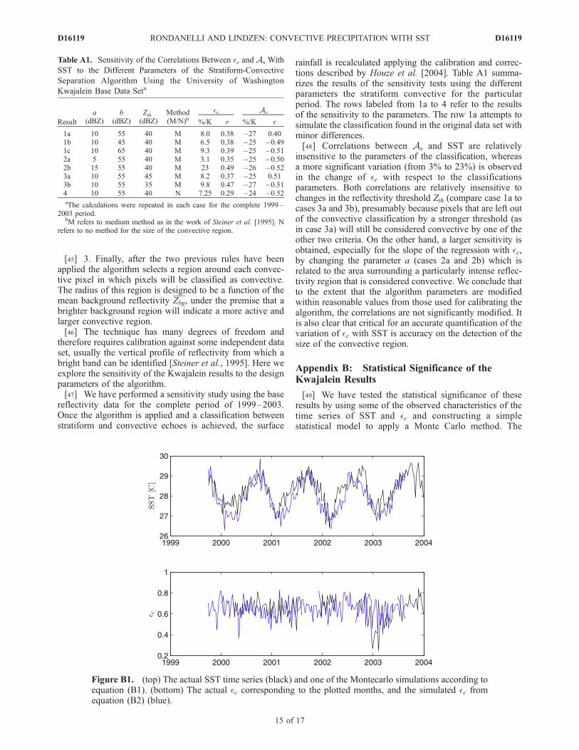
[49] We have tested the statistical significance of theseresults by using some of the observed characteristics of thetime series of SST and �c and constructing a simplestatistical model to apply a Monte Carlo method. The

Table A1. Sensitivity of the Correlations Between �c and As With

SST to the Different Parameters of the Stratiform-Convective

Separation Algorithm Using the University of Washington

Kwajalein Base Data Seta

Result

a(dBZ)

b(dBZ)

Zth(dBZ)

Method(M/N)b

�c As

%/K r %/K r

1a 10 55 40 M 8.0 0.38 �27 0.401b 10 45 40 M 6.5 0.38 �25 �0.491c 10 65 40 M 9.3 0.39 �25 �0.512a 5 55 40 M 3.1 0.35 �25 �0.502b 15 55 40 M 23 0.49 �26 �0.523a 10 55 45 M 8.2 0.37 �25 0.513b 10 55 35 M 9.8 0.47 �27 �0.514 10 55 40 N 7.25 0.29 �24 �0.52aThe calculations were repeated in each case for the complete 1999–

2003 period.bM refers to medium method as in the work of Steiner et al. [1995]. N

refers to no method for the size of the convective region.

Figure B1. (top) The actual SST time series (black) and one of the Montecarlo simulations according toequation (B1). (bottom) The actual �c corresponding to the plotted months, and the simulated �c fromequation (B2) (blue).

D16119 RONDANELLI AND LINDZEN: CONVECTIVE PRECIPITATION WITH SST

15 of 17

D16119

appropriate statistical model satisfies the null hypothesis H0:�c and SST are independent. Therefore the approach to testthe significance of the results will be to simulate throughthis statistical model calibrated through the observations,several pairs of values (�c

t,n,SSTt,n), where t = 1..tf are thetimes over which the series of measurements are taken (inthis case each t represents an 8-day period) and n is an indexthat indicates a single realization.[50] First, we define an idealized time series for the SST

based on the observed time series for SST in Kwajalein as,

SSTt;n ¼ SST þ cos 2pt=ty� �

þN t;n0;sSSTð Þ; ðB1Þ

where SST � 28 C and sSST � 0.3 C are the observed meanand standard deviation of the high pass filtered time seriesof SST. The time ty is the number of periods in a year so thecosine is meant to represent an annual cycle in SST with anamplitude of 1 C. N t,n is a realization from the normaldistribution meant to represent the high-frequency varia-bility of SST.[51] From these realizations of SST we can propose a

model for the behavior of �c consistent with the nullhypothesis. That is,

�t;nc ¼ �c þN t;n0; s�cð Þ ðB2Þ

We have pointed out that the variance of �c seems todecrease with SST (due in part to a decrease in thecomponent of the variance related to sampling) so that thestatistical significance determined from Monte Carlosimulations can be affected by whether we consider s�c asa constant or as a function of SST. So strictly speaking twoslightly different null hypotheses will be discussed: one in

which there is strict independence and the other one inwhich the dependence is constrained to appear only in theSST dependence of the variance. Figure B1 shows theoriginal time series for SST and �c and a single realizationof the model using the sampling dependence of thevariance.[52] For the cases in which there is an SST-dependent

variance a simple linear dependence is written,

s�c SSTð Þ ¼ SST0 � SSTð Þb þ s�c SST0ð Þ; ðB3Þ

with empirically derived values for b = 0.025 and s(SST0 =26 C) = 0.14.[53] Results for the Monte Carlo simulations of the

statistical process described in equation (B2) using a con-stant value for s�c equal to the empirically observed valueof 0.1 and a value of �c = 0.667 are shown in Figure B2 andB3. The results are for 10,000 realizations. The empiricaldistribution for both the slopes and the correlation coeffi-cients are centered around zero. Comparing the values forthe slope and the correlation coefficient obtained for the 8-day period averages, the null hypothesis is rejected underthis assumption at a relatively high significance level(slopes higher than 4.4% and correlation coefficients higherthan 0.22 are significant at the 0.1% level).[54] However, as previously mentioned, a test in which

the variance of the statistic �c is regarded as constant mightbe liberal in rejecting the null hypothesis. In fact, introduc-ing an SST dependence in the value of s�c according toequations (B2) and (B3), we observe that the distribution ofslopes and correlation coefficients becomes skewed towardpositive values. Therefore, a relatively larger value in theslopes and correlation coefficient is required (slopes higherthan 5.2% and correlation coefficients higher than 0.28 aresignificant at the 0.1% level). When comparing the value ofthe statistics related to these significance numbers to thevalues of the slope and correlation coefficient obtained in

Figure B2. Empirical distribution and cumulative fre-quency of the Monte Carlo simulations of the processes fora constant variance.

Figure B3. Same as Figure B2 but for an SST-dependentvariance according to (B3).

D16119 RONDANELLI AND LINDZEN: CONVECTIVE PRECIPITATION WITH SST

16 of 17

D16119

the corresponding observations (i.e., r = 0.42 and slope11.8%) we conclude that even in this case the nullhypothesis is rejected with a high confidence level. Similaranalyses performed for As show that the decrease with SSTis also statistically significant.

[55] Acknowledgments. The data used in this study were acquired aspart of the Tropical Rainfall Measuring Mission (TRMM). The algorithmswere developed by the TRMM Science Team. The data were processed bythe TRMM Science Data and Information System (TSDIS) and the TRMMOffice; they are archived and distributed by the Goddard Distributed ActiveArchive Center. TRMM is an international project jointly sponsored by theJapan National Space Development Agency (NASDA) and the U.S.National Aeronautics and Space Administration (NASA) Office of EarthSciences. This work was supported by DOE grant DE-FG02-01ER63257.We thank two anonymous reviewers for critically reading the manuscriptand making several useful remarks.

ReferencesAnderson, N., C. Grainger, and J. Stith (2005), Characteristics of strongupdrafts in precipitation systems over the central tropical Pacific Oceanand in the Amazon, J. Appl. Meteorol., 44(5), 731–738.

Awaka, J., T. Iguchi, H. Kumagai, and K. Okamoto (1997), Rain typeclassification algorithm for TRMM precipitation radar, IEEE Trans.Geosci. Remote Sens., 4, 1633–1635.

Bell, T., and P. Kundu (2000), Dependence of satellite sampling error onmonthly averaged rain rates: Comparison of simple models and recentstudies, J. Clim., 13(2), 449–462.

Berg, W., C. Kummerow, and C. Morales (2002), Differences between eastand west Pacific rainfall systems, J. Clim., 15(24), 3659–3672.

Betts, A. and Harshvardan (1987), Thermodynamic constraint on the cloudliquid water feedback in climate models, J. Geophys. Res., 92(D7),8483–8485.

Choi, Y.-S., and C.-H. Ho (2006), Radiative effect of Cirrus with differentoptical properties over the tropics in MODIS and CERES observations,Geophys. Res. Lett., 33, L21811, doi:10.1029/2006GL027403.

Churchill, D. D., and R. A. Houze (1984), Development and structure ofwinter monsoon cloud clusters on 10 December 1978, J. Atmos. Sci.,41(6), 933–960.

Clement, A., and B. Soden (2005), The sensitivity of the tropical-meanradiation budget, J. Clim., 18(16), 3189–3203.

Cotton, W., G. Alexander, R. Hertenstein, R. Walko, R. McAnelly, andM. Nicholls (1995), Cloud venting-A review and some new global annualestimates, Earth Sci. Rev., 39(3–4), 169–206.

Del Genio, A., and W. Kovari (2002), Climatic properties of tropical pre-cipitating convection under varying environmental conditions, J. Clim.,15(18), 2597–2615.

Del Genio, A. D., W. Kovari, M.-S. Yao, and J. Jonas (2005), Cumulusmicrophysics and climate sensitivity, J. Clim., 18(13), 2376–2387.

Doviak, R. J., and D. S. Zrnic (1993), Doppler Radar and Weather Ob-servations, 2nd ed., Academic, San Diego, Calif.

Emanuel, K. A., and R. T. Pierrehumbert (1996), Microphysical and dyna-mical control of tropospheric water vapor, in Clouds, Chemistry andClimate, vol. 135, edited by V. Ramanathan, pp. 17–28, Springer, Berlin.

Ferrier, B., J. Simpson, and W. Tao (1996), Factors responsible for preci-pitation efficiencies in midlatitude and tropical squall simulations, Mon.Weather Rev., 124(10), 2100–2125.

Gamache, J. F., and R. A. Houze (1983), Water budget of a mesoscaleconvective system in the tropics, J. Atmos. Sci., 40(7), 1835–1850.

Held, I., and B. Soden (2000), Water vapor feedback and global warming,Annu. Rev. Energy Environ., 25, 441–475.

Held, I., and B. Soden (2006), Robust responses of the hydrological cycleto global warming, J. Clim., 19(21), 5686–5699.

Heymsfield, G., B. Geerts, and L. Tian (2000), TRMM precipitation radarreflectivity profiles as comparedwith high-resolution airborne and ground-based radar measurements, J. Appl. Meteorol., 39(12), 2080–2102.

Houze, R. A. (1993), Cloud Dynamics, vol. 53, Academic, San Diego,Calif.

Houze, R. A. (1997), Stratiform precipitation in regions of convection: Ameteorological paradox?, Bull. Am. Meteorol. Soc., 78(10), 2179–2196.

Houze, R. A., Jr. (2004), Mesoscale convective systems, Rev. Geophys., 42,RG4003, doi:10.1029/2004RG000150.

Houze, R. A., S. Brodzik, C. Schumacher, S. E. Yuter, and C. R. Williams(2004), Uncertainties in oceanic radar rain maps at Kwajalein and im-plications for satellite validation, J. Appl. Meteorol., 43(8), 1114–1132.

Iguchi, T., T. Kozu, R. Meneghini, and J. Awaka (2000), Rain-profilingalgorithm for the TRMM precipitation radar, J. Appl. Meteorol., 39(12),2038–2052.

Johnson, R., T. Rickenbach, S. Rutledge, P. Ciesielski, and W. Schubert(1999), Trimodal characteristics of tropical convection, J. Clim., 12(8),2397–2418.

Kummerow, C., W. Barnes, T. Kozu, J. Shiue, and J. Simpson (1998), Thetropical rainfall measuring mission TRMM sensor package, J. Atmos.Oceanic Technol., 15, 809–817.

Lau, K., and H. Wu (2003), Warm rain processes over tropical oceans andclimate implications, Geophys. Res. Lett., 30(24), 2290, doi:10.1029/2003GL018567.

Lau, K., H. Wu, Y. Sud, and G. Walker (2005), Effects of cloud micro-physics on tropical atmospheric hydrologic processes and intraseasonalvariability, J. Clim., 18(22), 4731–4751.

Lin, B., B. A. Wielicki, P. Minnis, L. Chambers, K. M. Xu, Y. X. Hu, andA. Fan (2006), The effect of environmental conditions on tropical deepconvective systems observed from the TRMM satellite, J. Clim., 19(22),5745–5761.

Lindzen, R. S., M.-D. Chou, and A. Y. Hou (2001), Does the Earth have anadaptive infrared iris?, Bull. Am. Meteorol. Soc., 82(3), 417–432.

Rapp, A., C. Kummerow, W. Berg, and B. Griffith (2005), An evaluation ofthe proposed mechanism of the adaptive infrared iris hypothesis usingTRMM VIRS and PR measurements, J. Clim., 18(20), 4185–4194.

Renno, N., K. Emanuel, and P. Stone (1994), Radiative-convective modelwith an explicit hydrologic cycle: 1. Formulation and sensitivity to modelparameters, J. Geophys. Res., 99, 14,429 – 14,442, doi:10.1029/94JD00020.

Rutledge, S. A., and R. A. Houze (1987), A diagnostic modeling study ofthe trailing stratiform region of a midlatitude squall line, J. Atmos. Sci.,44(18), 2640–2656.

Schumacher, C., and R. A. Houze (2000), Comparison of radar data fromthe trmm satellite and kwajalein oceanic validation site, J. Appl. Meteorol.,39(12), 2151–2164.

Schumacher, C., and R. Houze (2003), Stratiform rain in the tropics as seenby the TRMM precipitation radar, J. Clim., 16(11), 1739–1756.

Schumacher, C., and R. Houze (2006), Stratiform precipitation productionover sub-Saharan Africa and the tropical East Atlantic as observed byTRMM, Q. J. R. Meteorol. Soc., 132(620), 2235–2255.

Spencer, R., W. Braswell, J. Christy, and J. Hnilo (2007), Cloud and radia-tion budget changes associated with tropical intraseasonal oscillations,Geophys. Res. Lett., 34, L11104, doi:10.1029/2007GL029844.

Steiner, M., R. A. Houze, and S. E. Yuter (1995), Climatological character-ization of three-dimensional storm structure from operational radar andrain gauge data, J. Appl. Meteorol., 34(9), 1978–2007.

Su, H., J. H. Jiang, Y. Gu, J. D. Neelin, J. W. Waters, B. H. Kahn, N. J.Livesey, and M. L. Santee (2008), Variations of tropical upper tropo-spheric clouds with sea surface temperature and implications for radiativeeffects, J. Geophys. Res., 113, D10211, doi:10.1029/2007JD009624.

Sun, D., and R. S. Lindzen (1993), Distribution of tropical troposphericwater vapor, J. Atmos. Sci., 50(12), 1643–1660.

TRMM Precipitation Radar Team (2005), Tropical Rainfall Measuring Mis-sion (TRMM) precipitation radar algorithm: Instruction manual for ver-sion 6, Jpn. Aerosp. Explor. Agency Natl. Aeronaut. and Space Admin.,Tokyo.

Yuter, S. E., and R. A. Houze (1997), Measurements of raindrop sizedistributions over the Pacific warm pool and implications for Z-R rela-tions, J. Appl. Meteorol., 36(7), 847–867.

�����������������������R. S. Lindzen and R. Rondanelli, Program in Atmosphere, Oceans, and

Climate, Massachusetts Institute of Technology, 54-1717, 77 MassachusettsAvenue, Cambridge, MA 02139, USA. (rrondane@mit.edu)

D16119 RONDANELLI AND LINDZEN: CONVECTIVE PRECIPITATION WITH SST

17 of 17

D16119