arX

iv:0

911.

3941

v1 [

phys

ics.

ao-p

h] 2

0 N

ov 2

009

I. INTRODUCTION

The importance of a reliable statistical definition of rain event resides in the possibility

of creating viable models for a great variety of hydrological applications: e.g. catchment

run-off, soil erosion and canopy losses [1]. Ecohydrologic studies rely on rain event modelling

to study the influence of the precipitation pulse dynamics on the vegetation architecture,

plant species interactions, and the cycling of organic matter and nutrients in arid and semi-

arid ecosystems [2, 3]. In spite of the widespread adoption of the rain event concept, a

proper non arbitrary statistical definition of rain event is still an open issue. The word

“event” has been used to indicate different things in different contexts, and a great variety

of techniques have been used for its definition. The most common criterion to define a rain

event is the Minimum Intra event Time (MIT): the MIT value separating two events ranges

from 15 min to 24 hours [1]. In many cases, the choice of a particular MIT is not related to

observed dynamical properties of the rainfall phenomenon but to a particular time scale of

the hydrological process considered: e.g. Lloyd et al. [4] use 3 h as MIT because it is the

estimated time for the canopy to dry, Bracken et al. [5] use MIT=12 h so that the ground

could dry between rain off events, while Aryal et al. [6] use 8 h as MIT because it is the

estimated time for highway surface depression to dry.

Recently, an alternative definition of rain event [7, 8, 9] has gained some recognition in

hydrological literature [10, 11, 12, 13, 14, 15, 16]. According to this new proposal a rain event

is identified by the occurrences of consecutive adjacent wet time intervals (the time intervals

being equal in duration to the instrument time resolution). We will refer to this method as

the Adjacent Wet Intervals (AWI) method. The adoption of this definition of rain event plays

a central role in what is the main claim of Peters et al. [7, 8, 9]: a dynamical “equivalence”

between the occurrence of rain events and that of avalanches in sand pile models. In this

case rain would have the same dynamical properties of self-organizing systems [17]. These

dynamical properties are commonly referred to, by the scientific community, with the term

Self Organized Criticality (SOC).

The MIT and AWI methods appear to be very different: the MIT method looks for the

lack of rain for a suitable interval of time, while the AWI method looks for time intervals

with a “continuous” presence of rain. We will compare both the MIT and AWI methods and

provide theoretical arguments to show that the two methods are “equivalent” and therefore

1

subject to the same arbitrariness: the choice of a minimum rainless interval in the MIT case,

and a particular time resolution of the instrument in the AWI case.

As a way out from the issue of arbitrariness, we propose here to focus on the dynamical

properties of the rainfall phenomenon and see if a particular time scale exists which could be

adopted as a physically meaningful (and thus not arbitrary) rainless period (time resolution)

in the MIT (AWI) case. There are two kinds of precipitation regimes: stratiform and

convective [18, 19]. The words stratiform and convective do not refer to the process of cloud

formation but to two distinct dynamical mechanisms of drop formation 1) stratiform: drops

are formed via condensation which is predominant in the case of small (<2m/s) updraft

velocity, and 2) convective: drops are formed via coalescence which is predominant in the

case of large (>2m/s) updraft velocity. The occurrence of convective precipitation at mid

latitudes is restricted to thunderstorm activity (isolated summer thunderstorm or Mesoscale

Convective Systems (MCS)), while both types of precipitation occur between the tropics in

spite of the fact that convection is the only mechanism of cloud formation, e.g.: [19].

Since physics laws are independent from the particular location on Earth, one expects that

two stratiform (convective) events must have some common statistical properties since the

rain drops were generated by the same physical mechanism. Note that the similarities we are

referring to are not similarity in the duration or depth of showers, although they might exists,

but similiraties in the statistical properties of inter drop time intervals and drop diameters.

In other words, it is not “how much” or“ how long” it rains which is similar (since orographic

condition and other particular meteorological factors may be relevant) but “how” it rains.

Newton’s law ~f=m~a tells us that body’s acceralation is always proportional to the applied

force, but the trajectory of a body will depend on the the peculiar force applied. Eventual

similar statistical properties of inter drop time intervals and drop diameters would be more

easily detected by direct study rather than through the observation of rainfall rates at a

given time resolution where things are complicated by the integration of the cube of the

drop diameters over an arbitrary time interval (time resolution). Ignaccolo et al. [20] have

shown that invariant statistical properties can be obtained for the inter drop time intervals

and drop diameters in the case of stratiform precipitation. We will use these properties

to propose a non arbitrary definition of rain event for the case of stratiform rain, and to

describe the internal variability of rain events.

In this manuscript, we use data from a Joss-Waldvogel (JW) disdrometer located at

2

Chilbolton, UK for which the precipitation is almost exclusively of stratiform kind. Our data

span a period of ∼2 years and are divided in 8 separate intervals of continuous observation

(all data details are in the Appendix A). In Section II, we review the properties of the

sequences of inter drop time intervals and drop diameters which are relevant to our purposes.

In Section III, we compare the MIT- and AWI-based definitions of event and show they are

“equivalent”. A non arbitrary criterion to define rain events is introduced in Section IV.

Moreover, we describe the intra event dynamical variability using the concepts of active and

quiescent phases. Finally, we draw our conclusions in Section V.

II. DROP-LIKE NATURE OF RAIN AND THE STATISTICAL PROPERTIES OF

STRATIFORM RAIN

Rainfall is discrete process being a collection of drops. Considering a small portion

of Earth’s surface, such as the collecting area of disdrometer or a rain gauge, rain can

be described mathematically as a sequence of couples (dj,τj), j=1,2,3,. . . . The symbol dj

indicates the diameter of the j-th drop, while τj is the time interval (inter drop time interval)

between the j-th and (j+1)-th drop. However, every instrument designed to detect rainfall

has a time resolution ∆>0: the instrument integration time. As a consequence, all inter drop

time intervals of duration τ<∆ are lost, and all inter drop time intervals of duration τ>∆

are detected as dry intervals, drought, of duration [τ/∆]×∆ or ([τ/∆]−1)×∆ ([.] indicates

the integer part) [20].

Let us consider as example ∆=1s. All inter drop time intervals τ<1s cannot be detected,

and the subsequent drops will “wet” the time intervals of duration ∆=1s containing them.

An inter drop time interval τ=1.3 s has 30% probability of resulting in a single dry interval

(drought of duration 1 s), and 70% probability of not being detected with the subsequent

drop wetting the time interval containing it. A value of τ=3.6 s will generate 3 consecutive

dry intervals (drought of 3 s) in 60% of the cases, and 2 consecutive dry intervals (drought 2 s)

in the remaining 40% of the cases. The above limitations are common to the great majority

of rainfall measuring instruments. The only exceptions are instruments with high temporal

resolutions (∼1 ms) such as the video disdrometer [21, 22, 23]. Thus, given a rainfall time

series one is able to calculate, in most cases, only the probability P (l∆) of observing l

consecutive dry intervals at resolution ∆. A better statistical accuracy is obtained using

3

the “survival” probability P (l∆): the probability of observing l or more consecutive dry

intervals at resolution ∆.

Neverthenless, it is possible to investigate the statistical properties of the inter drop

intervals also using data with a time resolution much larger than the one offered by video

disdrometer or particle spectrometer (∆≫1ms) such as the time resolution of our data ∆=10

s. In fact, it is possible to derive a formula describing the dependance of the probablity P (l∆)

on the probability density function ψ(τ) of having an inter drop time interval τ [20]. In the

limit τ≫∆ (l≫1), this dependence is rather simple:

P (l∆) ∝τ≫∆

ψ(l∆) ⇔ P (l∆) ∝τ≫∆

Ψ(l∆), (1)

where the symbol Ψ(τ) indicates the probability of having an inter drop time interval ≥τ

(survival probability).

A. Statistical properties of stratifrom rain

In the following, we briefly report some statistical properties of the sequence of couples

(dj,τj) in the case of stratiform rain derived in [20] to which we refer the reader for a detailed

discussion. The statistical properties relevant for the purposes of the present manuscript

are:

1) Drop diameters and inter drop time intervals are not independent as “large” inter

drop time intervals separate drops of “small” diameter. This conclusion was derived from

the observation of the conditional frequencies for a drop diameter given a specific value of

the preceeding inter drop time intervals. In particular, inter drop time intervals &10 s are

followed in >95% of the cases by a drop which diameter is ≤0.6 mm.

2) Large inter drop time intervals (τ>10s) are preceded/followed either by another large

inter drop time interval or by a sequence of few small (τ<10s) inter drop time intervals. In

this second case, the occurrence of 5 or less drops in the 10 seconds (a rate 0.5 drops per s)

following a large inter drop time interval is higly probable (≥95%).

3) Two different dynamical regimes of the rainfall phenomenon can be observed. These are

the quiescent and active phases. The contribution to the total cumulated flux of quiescent

phases is negligible (they are time intervals of sparse precipitation), while non quiescent

regions carry the bulk of the precipitated volume, hence they are “active”. Fig. 1 is a ∼3

4

days extract from our Chilbolton data showing the alternance of quiescent and active phases.

Note that the quiescent phase is not just what is commonly referred as a dry spell or drought

(e.g.: 5 days without precipitation are obviously a quiescent time interval) but it is a more

dynamically reach concept. For example, consider the time interval 15-25 h as depicted in

panel(b) of Fig. 1. If one hour resolution is adopted, the time interval 15-25 h will result in

a sequence of 10 consecutive wet intervals which could be considered as an event. However,

panel (b) of Fig. 1 shows that such a sequence of wet time intervals is constituted by two

quiescent phases (almost null flux increase) and an active phase in between (19-20 h) in

which a sharp increase of the cumulated flux occurs . The presence of quiescence and active

phases is a direct consequence of properties 1) and 2). Property 2) indicates the occurence

of time intervals of sparse precipitation since large inter drop time intervals are preceded

and followed by the occurrence of small rainfall rates ( ≤0.5 per second). While property

1) indicates the arrival of drops of small diameter (d≤0.6 mm) after large inter drop time

intervals genarating a negligible cumulated flux. As a matter of fact, one can use property 1)

and 2) to be label as quiescent all regions with a drop arrival rate ≤0.5 per second, and with

an average drop diameter ≤0.6 mm (see [20] for the detail implementation of this procedure).

The results of this filtering process is shown in Fig. 2. We see how the described filtering

procedure correctly indentifies the regions of null or almost null increase of the cumulated

flux: quiescent phases.

4) The probability density function of inter drop time intervals ψ(τ) has an inverse power

law regime in a certain range. We will define the borders of this interval in the next Section.

Note that using 1), 2) and 3), we can conclude that the inverse power law regime for the

frequency of inter drop time intervals is a dynamical charateristc of the quiescent phase.

III. ARBITRARY DEFINITIONS OF RAIN EVENT

Even if a physical identification of rain events based on meteorological considerations

accounting for atmospheric circulation and storm dynamics is preferable [4], a statistical

identification based on threshold criteria is widely used in hydrologic Literature for its sim-

plicity in applications.

5

A. The Minimum Inter event Time (MIT)

According to the MIT criterion, a rain event is the time interval in between the occurrence

of a dry period equal or larger in duration to a specific threshold: the minimum intra event

time or MIT. The range of MIT used in Literature is [15 min, 24 h]. The choice of a particular

MIT value influences the number of rain events, the distributions of event duration, depth,

and rain rate. Dunkerley [1] calculates empirical formulas linking the number of rain events,

the geometric mean event duration, the geometric mean event volume, the geometric mean

event rain rate, and the geometric mean inter event time to the MIT values. Hereby, we

plot in Figs. 3 and 4 the survival probabilities PMIT(θ), the probability of observing a rain

event of duration ≥θ, and PMIT(w), the probability of observing a rain event depth ≥w for

different MIT values T . The shapes of the probabilities PMIT(θ) and PMIT(w) heavily depend

on the particular value T .

B. Adjacent Wet Intervals (AWI)

According to the proposal of Peters et al. [7, 8, 9], a rain event is a sequence of consecutive

“wet” (precipitation occurred) time intervals of duration ∆: the instrument resolution.

Note however that given a rainfall time series with time resolution ∆, one can build the

corresponding time series for resolutions which are multiple of the time resolution (2∆, 3∆,

. . . ). As for the MIT case, we plot in Figs. 3 and 4 the survival probabilities P AWI(θ) and

P AWI(w) relative to the rain event duration and rain event depth. Also in this case, we notice

a marked dependence on the time resolution ∆. The dependence on the time resolution ∆

observed in Figs. 3 and 4 for the survival probabilities P AWI(θ) and P AWI(w) casts doubts

on the claims that a proper theoretical framework for the rainfall phenomenon is the Self

Organized Criticality [9]. In fact the claim is based on the observed inverse power law for the

survival probability of observing a depth of duration w, in the case ∆=1min. This behavior

is typical of self organizing systems such as Earth’s crust under stress and deformation which

is why Peters et al. refer to the inverse power law behavior of rain event depths as rain’s

Gutenberg-Richter law [24]. Fig. 4 shows that one could fit an inverse power law function

to the survival probability P AWI(w) relative to the resolutions ∆=10 s and ∆=1 min and

obtain (in the range [0.001,1] mm) two rather different exponents : µ=0.48 and µ=0.33

6

respectively. The exponents of the probability density function ψ(τ) are obtained adding 1

to the exponent of the survival probability Ψ(τ). Moreover, for larger time resolutions the

inverse power law character of the survival probability P AWI(w) becomes less evident and

the eventual exponent gets closer to zero: µ=0.14, µ=0.09, and µ=0.08 for ∆=10 min, 1 h,

and 3 h (the range [0.001,0.1]mm was used for these three last fits).

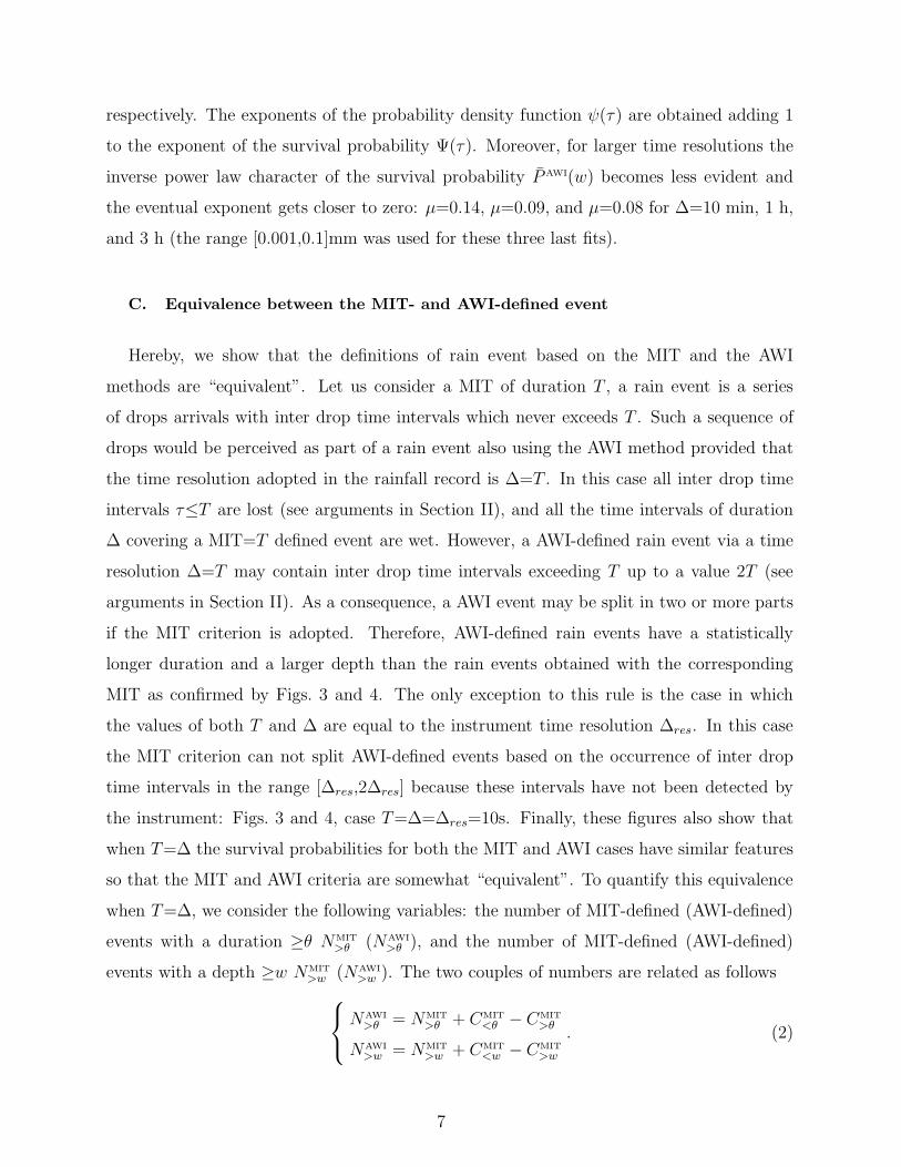
C. Equivalence between the MIT- and AWI-defined event

Hereby, we show that the definitions of rain event based on the MIT and the AWI

methods are “equivalent”. Let us consider a MIT of duration T , a rain event is a series

of drops arrivals with inter drop time intervals which never exceeds T . Such a sequence of

drops would be perceived as part of a rain event also using the AWI method provided that

the time resolution adopted in the rainfall record is ∆=T . In this case all inter drop time

intervals τ≤T are lost (see arguments in Section II), and all the time intervals of duration

∆ covering a MIT=T defined event are wet. However, a AWI-defined rain event via a time

resolution ∆=T may contain inter drop time intervals exceeding T up to a value 2T (see

arguments in Section II). As a consequence, a AWI event may be split in two or more parts

if the MIT criterion is adopted. Therefore, AWI-defined rain events have a statistically

longer duration and a larger depth than the rain events obtained with the corresponding

MIT as confirmed by Figs. 3 and 4. The only exception to this rule is the case in which

the values of both T and ∆ are equal to the instrument time resolution ∆res. In this case

the MIT criterion can not split AWI-defined events based on the occurrence of inter drop

time intervals in the range [∆res,2∆res] because these intervals have not been detected by

the instrument: Figs. 3 and 4, case T=∆=∆res=10s. Finally, these figures also show that

when T=∆ the survival probabilities for both the MIT and AWI cases have similar features

so that the MIT and AWI criteria are somewhat “equivalent”. To quantify this equivalence

when T=∆, we consider the following variables: the number of MIT-defined (AWI-defined)

events with a duration ≥θ NMIT

>θ (NAWI

>θ ), and the number of MIT-defined (AWI-defined)

events with a depth ≥w NMIT

>w (NAWI

>w ). The two couples of numbers are related as follows

NAWI

>θ = NMIT

>θ + CMIT

<θ − CMIT

>θ

NAWI

>w = NMIT

>w + CMIT

<w − CMIT

>w

. (2)

7

The symbol CMIT

<θ (CMIT

<w ) in Eq. (2) is the number of events gained via connection of two

or more MIT events which singularly have all a duration (depth) <θ (<w). Similarly, CMIT

>θ

(CMIT

>w ) is the number of events lost via connection of two or more MIT events which singularly

had already a duration (depth) ≥θ (≥w). The two relations in Eq. (2) can be transformed

in relations among the corresponding survival probabilities if the r.h.s. and l.h.s of both

relations are multiplied by the constant factor NAWI

E /(NMIT

E NAWI

E ), where NMIT

E (NAWI

E ) is the

total number of MIT (AWI) events. After some algebra, we obtain

P AWI(θ) =NMIT

E

NAWI

E

(

PMIT(θ) + cMIT

<θ − cMIT

>θ

)

P AWI(w) =NMIT

E

NAWI

E

(

PMIT(w) + cMIT

<w − cMIT

>w

)

. (3)

The symbol cMIT

<θ (cMIT

>θ ,cMIT

>w , cMIT

<w ) is the number CMIT

<θ (CMIT

>θ , CMIT

<w , CMIT

>w ) divided by the total

number of MIT events NMIT

E . Eq. (3) shows that if we disregard the correction terms cMIT

<θ ,

cMIT

>θ , cMIT

>w , and cMIT

<w the AWI survival probabilities P AWI(θ) and P AWI(w) are proportional

to the MIT survival probabilities PMIT(θ) and PMIT(w). Thus in a log-log plot the two

kind of distributions will differ by a constant factor which explains the “similitude” between

MIT and AWI statistics observed in Figs. 3 and 4. To further test this conjecture we

plot in Figs. 5 and 6 the survival probability P AWI(θ) (P AWI(w)) with the rescaled survival

probability (NMIT

E /NAWI

E )PMIT(θ) ((NMIT

E /NAWI

E )PMIT(w)). Figs. 5 and 6 confirm that the

statistical properties of MIT- and AWI-defined events are “equivalent”: the correction terms

in Eq. (3) do no alter dramatically the shape of the survival probability functions.

IV. A NON ARBITRARY DEFINITION OF RAIN EVENT

In his review work [1], Dunkerley shows the great variability in the MIT value used to

define an event, and also how in many cases events are defined but the criteria are not

reported. Another issue related to the particular value of MIT adopted is the intra event

“variability”: namely the fact that an event is not characterized by the continuous presence

of rain, but it is mostly rainless. About 75% of the event duration is found to be rainless by

[25]. Hereby, we show how to address these important questions it is necessary to focus on

the dynamical properties of the rainfall phenomenon.

In Section II and Section IIA, we have discussed the properties of the sequence of the

couples (dj,τj) and shown that two phases of rainfall phenomenon can be identified: a quies-

8

cent one and an active one. These findings and Eq. (1) allow us a dynamically interpretation

of the survival probability P (l∆)

Let us consider the extreme values of the inter drop time intervals (τ→∞). The shape

of the survival probability P (l∆) for extreme values (l≫1) is a signature of the particular

meteorological condition of the location in which data are gathered (e.g.: arid/non arid

region). Thus we refer to this region as the meteorological region. The problem of a “proper”

choice of MIT (or time interval ∆ in the AWI case) is related to where to locate the left

border of the meteorological region. As we move from +∞ to smaller values of inter drop

time interval, we cross the border between the inter-storm dynamics (meteorological region)

and the intra-storm dynamics (different showers belonging to the same synoptic event).

Where to locate this border? We think that the emergence of a power law regime for the

inter drop time intervals suggests a clear (non-arbitrary) “dynamical” choice.

We adopt the following operational method for locating this border. We fit with an inverse

power law function the survival probability P (l∆) in the range [>3 min, 1 h], corresponding

a range [>18, 360] for l, given the resolution ∆=∆res=10 s of our data. The notation >3

min (>18) indicates that the left border is taken to be 3 min or more: we consider 3 min

as the minimum value for which Eq. (1) is satisfied. However, there are cases for which the

survival probability P (l∆) cannot be yet consider to have an inverse power law behavior

(no approximate straight line in a log-log plot) for l=18 and larger values of l (∼30-40) are

chosen since fit accuracy is dependent on a proper choice for the minimum value for which

the inverse power law holds [26]. Moreover, we choose l=360 (1 hour) for the right border

of the fitting region, a value that is smaller of what is the expected (by visual inspection)

limit of validity of the power law behavior. Once the fit is performed, we consider a ±10%

difference from the value of the fitting curve as an indication of departure from the inverse

power law regime. Thus, we look at values of l>360 and seek the occurrence of at least 5

consecutive data points outside the 10% error bar to declare as “over” the inverse power law

regime. With this method the power law regime for the survival probability P (l∆) relative

to the time interval of continuous observation from 04/01/2003 to 11/03/2003 occurs in the

[3 min, 2 h] range as shown in Fig. 7. Finally, we check if the calculation of the inverse

power law range may be affected by lack of statistics. If N droughts are present in a raifall

record, which is the maximum value lmax for the survival probability P (l∆) to be statistically

reasonable? With N samples the smallest “probability” detectable is 1/N . However one

9

TABLE I: The range of validity of the inverse power law regime, the number N of droughts, and

the values lmax∆ denoting the limit up to which the survival probability P (l∆) can be considered

statistically sound for all the 8 intervals of continuous observation in our data.

Time interval of observation Range N lmax×∆

04/01/03 – 11/03/03 3 min - 2 h 118417 69.4 h

11/05/03 – 01/05/04 6 min - 1.5 h 17879 22.2 h

01/08/04 – 01/20/04 6 min - 32 min 10875 32 min

01/24/04 – 05/11/04 6 min - 4 h 40781 24.2 h

05/14/04 – 07/17/04 3 min - 2,77 h 15519 2.77 h

07/19/04 – 08/02/04 3 min - 1.61 h 2857 1.61 h

08/04/04 – 08/19/04 3 min - 53 min 4612 53 min

12/10/04 – 02/28/05 6 min - 1 h 4401 2.55 h

cannot define lmax as the values for which the following equality P (lmax∆)=1/N holds: this

is equivalent to say that all values of the survival probability are statistically sound. A

more realistic and reasonable assumption can be done using the law of large numbers and

in particular the Chebyshev’s inequality [27]. Let us consider an integer K<N and the

corresponding value lK for which the theoretical expected probability of having droughts

equal or larger in value than lk∆ is K/N . According to the Chebyshev’s inequality,

Pr

P (lK∆) >= 2K

N

≤1

K

(

1 −K

N

)

. (4)

The value 1/K(1-K/N)≃1/K if K≪N is the maximum possible value for the probability

(Pr) of observing, due to the finiteness of the sample (N<∞), a value of the survival prob-

ability P (lK∆) which is at least the double (2K/N) of the expected one. If we consider

K=10≪N and the corresponding l10, Eq. (4) says that the survival probability P (l10∆) can

be considered reasonably close to the expected theoretical value. In fact, there is probability

=10% that the observed value of P (l10∆) is wrong by a factor 2 or more. Thus we set

lmax=l10: the dashed box in Fig. 7 indicates the region of “poor” statistics in the case of

the time interval from 04/01/2003 to 11/03/2003. Table 1 reports the values of lmax∆ for

all 8 time intervals of continuous observation available to us together with the number N

of droughts in the interval and the estimated range of validity of the inverse power law.

Of the 8 time intervals of continuous observation only 3 (04/01/03 – 11/03/03, 11/05/03

10

– 01/05/04/, and 01/24/04 – 05/11/04) have an accuracy (value of lmax∆) for the survival

probability which is well above 20 h. The remaining intervals have an accuracy which does

not permit to accurately locate the end of the power law regime. Considering the only 3

intervals with reasonable accuracy, we have for the limit of validity of the inverse power law

regime the following values: 1.5, 2, and 4 h with an average value of 2.5 h.

Crossing, from right to left, the mark indicating the end of the inverse power law regime,

we move from the meteorological region into the intra-storm quiescent region which from

now on we will refer simply as the quiescent region. Moving to even smaller values of inter

drop time intervals, we reach the intra-storm active region, from now on simply the active

region. This transition cannot be observed with our data since the instrument resolution

is ∆res=10 s. However, we know that active regions are characterized by a drop arrival

rate ≫0.5 per second (Section 2.1). A drop arrival rate of 5 per second translates into an

average inter drop time interval of 0.2 s. Moreover, we know (Section 2.1) that inter drop

time intervals ∼10s belong to quiescent phases. Therefore, an educated guess for the time

interval where to locate the transition from the quiescent phase into the active phase is [∼1,

∼10] s. This guess is confirmed by the plot of the probability density function ψ(τ) of inter

drop time interval in Lavergnat et al. [21, 22] (obtained with an optic disdrometer which

time resolution is ∆res=1 ms). The plot shows an inverse power law regime to emerge for

inter drop time intervals τ&5 s. Fig. 8 shows the three dynamical regions together with

the probability P∆(l∆) which is proportional, Eq. (1), to the survival probability of inter

drop time intervals Ψ(τ). The vertical lines indicate the range [1.5, 4] h. The other solid

lines indicate “qualitatively” the probability for a given inter drop time interval to belong

to a given dynamical region. A more “quantitative” description of these curves cannot

be achieved with the data at our disposal: 1) for the transition between quiescent and

meteorological region we need the synoptic information for the period of observation, 2) for

the transition between the active and quiescent region we need a better instrument’s time

resolution.

A. Intra event variability: active and quiescent phases

Each event is composed by a non overlapping sequence of quiescent and active phases

(Fig. 2). To describe the intra event dynamical variability, we decide to calculate for each

11

event which percentage of its duration and depth is due to active phases. We consider

MIT=3h and all the 8 time intervals of continuous observation at our disposal (Appendix

A) for a total of 262 events. The identification of quiescent and active phases inside each

event is done using the same quiescent filter procedure used in [20]. For each event, we

calculate the percentage %dur of the event duration which is covered by active phases, and

the percentage %dep of the event depth which is due to active phases. Then we calculate

the number n(%dep,%dur) of events with a given %dur and %dep, and the number n(%dur)

(n(%dep)) of events with a given %dur (%dep). The results are shown in panels (a) and

(b) of Fig. 9 respectively. The distribution of the number n(%dep,%dur) of events with a

given %dur and %dep is roughly concentrated, panel (a), on a L-shaped region (the region

of small values of %dur and the region of large values of %dep). This is confirmed by the

plot of the numbers n(%dur) and n(%dep) of events with a given %dur and %dep, panel (b).

Of the 262 events available, 62 have 0 active %dep and %dur: black square in (0,0) in panel

(a), and left peak of the number n(%dep) in panel (b). These events are produced by two

different kinds of sequential ordering of inter drop time intervals τ : 1) a τ>MIT followed by

a τ<MIT followed by a τ>MIT or 2) a τ>MIT followed by a quiescent phase followed by a

τ>MIT. The first kind of sequence generates events constituted by a single drop, the second

kind generates events composed by a single quiescent phase with negligible depth. The great

majority of the remaining events (172 of 200) have an active %dep>80% and a %dur which

is mostly (151 of 172) less than 40%, as indicated by the plot of n(%dur) and n(%dep) in

panel (b). The left peak of n(%dur), panel (b), is given by the 62 events with 0 active

%dep and %dur, and by the events with %dur≤5% and variable %dep (one of the arms

of the L-shaped region formed by the gray scale squares in panel (a)). Finally, the region

of the (%dur,%dep) plane defined by the condition %dep≥80% (right peak of n(%dep) in

panel (b)) is the region where all the “relevant” events (event depth &1mm) are located as

revealed by the plot of the event depth versus the %dur and %dep variables (vertical lines on

panel (a)). Note how the depth of the event with %dur≤5% and %dep≤80% is so negligible

that they are not resolved by the adopted scale for the z-axis in panel (a).

12

V. CONCLUSIONS

The question of “what a rain event is” has not been a simple one to answer in a statistical

way. A plethora of methods have been proposed all of which affected by a degree of arbitrari-

ness [1]. We compare two methods for defining rain events: 1) the MIT method, the most

common [1], is based on defining a minimum rainless time interval T separating two events.

2) The AWI method which is based on the occurrence of consecutive wet intervals of equal

duration ∆. The statistical properties of the rain event duration and rain event depth are

highly dependent from the particular value of T (MIT-events) and ∆ (AWI-events) chosen

as shown by the plots of the survival probabilities (Figs. 3 and 4 in Section 3.1 and 3.2). If

for a given value of the parameter T (∆) one could say that an inverse power law beahvior

with scaling parameter µ exists for the survival probability of rain event duration and/or

rain event depth, the same is not true for a different value of the parameter T (∆): either

the scaling parameter µ is sensibly different or there is no inverse power law regime. Conse-

quently, claims made using survival probabilities (and/or probability density functions) for

a particular value of T (∆) should be considered void or doubtful at best. E.g., we doubt

the conclusion reached by Peters et al. [9]: inverse power law behavior for the probability

of observing a rain event with depth w, in the case ∆=1min, ⇒ Gutenberg-Richter law for

rainfall ⇒ rainfall is an example of SOC.

Moreover, we show that the MIT and the AWI methods are equivalent (if T=∆) since the

corresponding survival probabilities for the rain event duration and depth have similar be-

havior (Eq. (2), Eq. (3), and Figs. 5 and 6 of Section 3.3). This is so because the occurrence

of adjacent wet intervals at time resolution ∆ is related to the NOT occurrence of inter drop

time intervals >∆ (Section II). It is worth noting that the equivalence between the MIT and

AWI methods is not perceived as such in literature: the AWI method is presented as alter-

native method reflecting the “burst”-like and scaling properties of the rainfall phenomenon,

e.g. [13, 15]. This misconception is paired, in our opinion, with a lack of recognition of the

drop-like nature of the rainfall phenomenon which result in the absence of detailed studies

about the properties of the sequence of couples (dj ,τj), drop diameter and inter drop time

interval: [20, 21, 22] being, to the best of our knowledge, the only exceptions.

Yet, the statistical properties of the sequence of inter drop time interval and drop diameter

(properties 1), 2), 3), and 4) of Section IIA) play a fundamental role also in answering the

13

important question of what constitutes a rain event. We propose to use the ending time

of the inverse power law regime present in the probability density function of inter drop

time intervals ψ(τ) as the time T (resolution ∆) to adopt in the MIT (AWI) method. With

the data at our disposal, we estimate (table 1) the ending time of the inverse power law

regime to be in the range [1.5,4]h. Some considerations about this proposal are in order. 1)

The proposal takes in account only the dynamics of the rainfall phenomenon and completely

ignores, as it should be, any particular time scale relative to any other hydrological processes,

e.g. catchment/runoff or canopy losses, which do not have any relevance for the occurrence

of rain. This is not a limitation for the possible application of the proposed method. On

the contrary, it is a strength: considering only the time scale of the particular hydrological

application, while ignoring those relative to the rain and the possible complicated interplay

of both, is not a recipe for success. 2) We consider this proposal valid only for stratiform

rain. The term stratiform has to be intended as in [19]: updraft velocity in the clouds are

typically less than 2 m/s leading to drop formation via condensation. This is the typical rain

regime for Chilbolton, UK, and in general the predominant one at mid-latitudes. 3) We deem

this proposal to be non arbitrary because the inverse power law regime for the probability

density function of inter drop time interval is a genuine dynamical properties of stratiform

rain. In fact the inverse power law regime is observed in all 8 time intervals of continuous

observation, spanning almost 2 years, at Chilbolton (see [20]) but also in other mid-latitude

locations: Germany, France and Italy ([20] and references therein). 4) The criterion hereby

discussed for a non arbitrary definition of rain event in the case of stratiform rain may have

also some applicability in the case of convective rain, since stratiform precipitation occurrs

inside “dying” cell of convective storms [19].

Finally in Section 4.1, we use the concepts of quiescent and active phases to describe the

internal dynamical variability of a rain event. Rain events are mostly occupied by quiescent

phases which precedes and/or follows “showers” responsible for the bulk of the event depth

(active phases). There are many possible of ways of describing the rain events propeties and

varability, e.g. quaterly volumes. A detailed comparison between our description of rain

events in terms of quiescent and active phases and other metodology is beyond the scope of

the present manuscript.

14

APPENDIX A: CHILBOLTON DATA

The data used in this manuscript are collected at Chilbolton (UK) using a Joss-Waldvogel

impact disdrometer RD-69 [28], and provided by the British Atmospheric Data Centre. Pre-

cipitation at this location was monitored for a time interval of ∼2 years. However, some

values are indicated as missing, and the data were carefully inspected to remove chunks were

no value was reported. After this inspection, 8 different time intervals of continuous observa-

tion were identified: from 04/01/2003 to 11/03/2003, from 11/05/2003 to 01/05/2004, from

01/08/2004 to 01/20/2004, from 01/24/2004 to 05/11/2004, from 05/14/2004 to 07/17/2004,

from 07/19/2004 to 08/02/2004, from 08/04/2004 to 08/19/2004, and from 12/10/2004 to

02/28/2005. The instrument has a collecting area A=50cm2 and provides every ∆=10s

the drop diameter count for 127 different diameter classes (channels). The lower limit of a

diameter class is defined by the following relation [29],

dci=

[

10(1−α(127−i))

γ

]β

, (A1)

where i is the diameter class index, dcithe lower boundary of the i-th class, α=0.014253,

β=0.6803, and γ=0.94. Thus, the range of observed diameters is [0.3mm,5mm]. Eq. (A1)

makes the diameter classes uniformly spaced in a logarithmic scale so that small drops are

classified through finer classes than those used for large drops. The interested reader can find

a detailed discussion on impact disdrometers and their limitations in [28, 30, 31, 32, 33],while

more detailed information about the instrument at Chilbolton can be found in [29].

15

0123

01

10100

15

25125

0 10 20 30 40 50 60 70 0

10

20d– (m

m)

ln

(a)

Cum

ulat

ed fl

ux (m

m)

0123

01

10100

15

25125

0 5 10 15 20 25 30 0

2

4

6

d– (mm

)l

n

(b)

Cum

ulat

ed fl

ux (m

m)

0123

01

10100

15

25125

30 40 50 5

15

25

time (hours)

d– (mm

)l

n

(c)

Cum

ulat

ed fl

ux (m

m)

FIG. 1: A ∼3 days extract from our data set. For each time interval ∆=10 s (instrument resolution),

we plot the number n of drops fallen, and the average drop diameter d in the interval. Moreover,

we plot the number l of consecutive dry intervals (droughts of duration l∆). A drought of duration

100∆ is represented by a horizontal bar of 100 data points at the “100” level. Each wet interval

(interval occupied at least by one drop) is represented as a drought of null duration: “0” level.

Finally the continuous line represents the cumulated flux. Panel (a) shows the above mentioned

quantities for the entire duration of the extract (70 hours), panel (b) zooms on the first 30 hours,

and panel (c) zooms on the 30 to 52 hours range. Note how the properties 1) and 2) described in

Section IIA create extended regions in which precipitation occurs without a detectable increase of

16

01230123

0 10 20 30 40 50 60 70 0

10

20

d– (mm

)(a)

Cum

ulat

ed fl

ux (m

m)

01230123

0 5 10 15 20 25 30 0

2

4

6

d– (mm

)

(b)

Cum

ulat

ed fl

ux (m

m)

01230123

30 40 50 5

15

25

time (hours)

d– (mm

)

(c)

Cum

ulat

ed fl

ux (m

m)

FIG. 2: The average diameter d in a time interval of duration ∆=10s and the cumulated flux

before (bottom half dots and solid line) and after (upper half dots and dashed line) removing

the quiescent phases as a function of time. The gray shaded areas provide visual aid highlighting

quiescent regions. Panel (a), the entire 70 hours of observation, panel(b) zooms in to the first 30

hours, and panel (c) zooms on the 30 to 52 hours range.

17

10-6

10-5

10-4

10-3

10-2

10-1

1 10 100 1000 10000 100000

P_ MIT(θ

), P_ A

WI (θ

)

θ (unit of 10s)

1 min 1 hour 1 day

T=∆=10s

T=∆=1min

T=∆=5min

T=∆=10min

T=∆=1h

T=∆=3h

1

FIG. 3: The survival probabilities PMIT(θ) (squares) and P

AWI(θ) (solid lines) for different values of

T (MIT method) and time interval ∆ (AWI method) respectively. The time interval of continuous

observation used for this figure is the one from 01/24/2004 to 05/11/2004.

18

10-6

10-5

10-4

10-3

10-2

10-1

0.0001 0.001 0.01 0.1 1 10 100

P_ MIT(w

), P_ A

WI (w

)

w (mm)

1

T=∆=10s

T=∆=1min

T=∆=5min

T=∆=10min

T=∆=1h

T=∆=3h

FIG. 4: The survival probabilities PMIT(w) (squares) and P

AWI(w) (solid lines) for different values of

T (MIT method) and time interval ∆ (AWI method) respectively. The time interval of continuous

observation used for this figure is the one from 01/24/2004 to 05/11/2004.

19

10-6

10-5

10-4

10-3

10-2

10-1

1 10 100 1000 10000 100000

(NM

IT E /

NA

WI

E )

P_ MIT(θ

), P_ A

WI (θ

)

θ (unit of 10s)

1 min 1 hour 1 day

1

T=∆=1min

T=∆=5min

T=∆=10min

T=∆=1h

T=∆=3h

FIG. 5: The survival probability PAWI(θ) (squares) and the function (NMIT

E /NAWI

E ) PMIT(θ) (solid

lines) for different values of T (MIT method) and time interval ∆ (AWI method) respectively.

The time interval of continuous observation used for this figure is the one from 01/24/2004 to

05/11/2004.

20

10-5

10-4

10-3

10-2

10-1

0.0001 0.001 0.01 0.1 1 10 100

(NM

IT E /

NA

WI

E )

P_ MIT(w

), P_ A

WI (w

)

w (mm)

1

T=∆=1min

T=∆=5min

T=∆=10min

T=∆=1h

T=∆=3h

FIG. 6: The survival probability PAWI(w) (squares) and the function (NMIT

E /NAWI

E ) PMIT(w) (solid

lines) for different values of T (MIT method) and time interval ∆ (AWI method) respectively.

The time interval of continuous observation used for this figure is the one from 01/24/2004 to

05/11/2004.

21

10-5

10-4

10-3

10-2

10-1

1 10 100 1000 10000 100000

P_ MIT(l∆

)

l∆ (unit of 10s)

±1

3 min 1 hour

poor statistics

10% curve

FIG. 7: Log-log plot of the survival probability P (l∆) for the time interval of continuous observation

that goes from 04/01/2003 to 11/03/2003 (squares). The solid lines are indicate an error barof

±10% with respect to the inverse power law fitting curve in the range 3 min - 1 h. Finally the box

in the bottom right corner (dashed lines) indicate he region of poor statistics, see Eq. (4).

22

10-5

10-4

10-3

10-2

10-1

10-3 10-2 10-1 10+0 10+1 10+2 10+3 10+4 10+5 10+6 10+7

P_ (l∆)

l∆ (s)

1

active quiescent meteo

1 min 1 hour 1 day

FIG. 8: Log-log plot of the survival probability P (l∆) for the time interval of continuous observation

that goes from 04/01/2003 to 11/03/2003 (squares). The vertical lines indicate the proposed range

for the “proper” choice of MIT. The other solid lines indicate qualitatively the probability (not

normalized for better clarity) for an inter drop time interval τ to belong to each of the three

dynamical phases of the rainfall phenomenon.

23

0 20 40 60 80 100 0 20 40 60 80 100

0 15 30 45 60

even

t dep

th (

mm

)

%dep %dur

n(%dep,%dur)

(a)

even

t dep

th (

mm

)

0 10 20 30 40 50 60 70

0 20 40 60 80

100 120 140

0 20 40 60 80 100

n(%

dur)

, n(%

dep)

%dur, %dep

(b)

0 10 20 30 40 50 60 70

FIG. 9: panel (a). The number n(%dep,%dur) of events for which the active phases cover %dur of

the total duration and %dep of the total depth (gray scale squares) calculated using a 5% bin for

both %dep and %dur. The depth of an event versus the percentage of duration %dur and depth

%dep due to active phases (vertical lines). Panel(b) The plot of the number of events n(%dur)

with a given %dur value (dashed line), and the number n(%dep) of events with a given %dep value

(solid lines).

24

[1] D. Dunkerley, Identifying individual rain events from pluviograph records: a review with

analysis of data from an Australian dryland site, Hydrological Processes 22 (26) (2008) 5024–

5036. doi:10.1002/hyp.7122.

[2] S. L. Collins, R. L. Sinsabaugh, C. Crenshaw, L. Green, A. Porras-Alfaro, M. Stursova, L. H.

Zeglin, Pulse dynamics and microbial processes in aridland ecosystem, Journal of Ecology

96 (3) (2008) 413–420.

[3] S. Schwinning, O. E. Sala, M. E. Loik, E. J. R., Thresholds, memory, and seasonality: under-

standing pulse dynamics in arid/semi-arid ecosystems, Oecologia 141 (2004) 191–193.

[4] C. Lloyd, The temporal distribution of Amazonian rainfall and its implications for forest

interception, Quarterly Journal of the Royal Meteorological Society 116 (496) (1990) 1487–

1494.

[5] L. Bracken, N. Coxi, J. Shannon, The relationship between rainfall inputs and flood generation

in south-east Spain, Hydrological Processes 22 (5) (2008) 683–696. doi:10.1002/hyp.6641.

[6] H. Aryal, R. K.and Furumai, F. Nakajima, H. K. P. K. Jinadasa, The role of inter-event time

definition and recovery of initial/depression loss for theaccuracy in quantitative simulations

of highway runoff, Urban Water Journal 4 (207) 53–58.

[7] O. Peters, C. Hertlein, K. Christensen, A complexity view of rainfall, Physical Review Letters

88 (1) (2002) 1–4.

[8] O. Peters, K. Christensen, Rain: Relaxations in the sky, Physical Review E 66 (3).

[9] O. Peters, K. Christensen, Rain viewed as relaxational events, Journal of Hydrology 328 (1-2)

(2006) 46–55.

[10] R. Andrade, Exact solution for the self-organized critical rainfall model, Brazilian Journal of

Physics 33 (3) (2003) 437–442.

[11] C. M. Aegerter, A sandpile model for the distribution of rainfall?, Physica A 319 (2003) 1–10.

[12] R. Dickman, Fractal rain distributions and chaotic advection, Brazilian Journal of Physics

34 (2A, Sp. Iss. SI) (2004) 337–346.

[13] L. Telesca, G. Colangelo, V. Lapenna, M. Macchiato, On the scaling behavior of rain event

sequence recorded in Basilicata region (Southern Italy), JOURNAL OF HYDROLOGY 296 (1-

4) (2004) 234–240.

25

[14] R. Bove, V. Pelino, L. De Leonibus, MComplexity in rainfall phenomena, Communications in

Nonlinear Science and Numerical Simulation 11 (2006) 678–684.

[15] L. Telesca, V. Lapenna, E. Scalcione, D. Summa, Searching for time-scaling fea-

tures in rainfall sequences, CHAOS SOLITONS & FRACTALS 32 (1) (2007) 35–41.

doi:10.1016/j.chaos.2005.10.078.

[16] A. P. Garcia-Marin, F. J. Jimenez-Hornero, J. L. Ayuso-Munoz, Multifractal analysis as a tool

for validating a rainfall model, HYDROLOGICAL PROCESSES 22 (14) (2008) 2672–2688.

doi:10.1002/hyp.6864.

[17] P. Bak, C. Tang, K. Wiesenfeld, Self-organized criticality: an explanation of 1/f noise, Physical

Review Letters 59 (1987) 381–284.

[18] R. A. Houze, Cloud dynamics, Academic Press, San Diego, 1993.

[19] R. A. Houze, Stratiform precipitation in regions of convection: a meteorological paradox?,

Bulletin of the Ameraican Meteorological Society 78 (10) (1997) 2179–2196.

[20] M. Ignaccolo, C. De Michele, S. Bianco, The Droplike Nature of Rain and Its

Invariant Statistical Properties, Journal of Hydrometeorology 10 (1) (2009) 79–95.

doi:10.1175/2008JHM975.1.

[21] J. Lavergnat, P. Gole, A stochastic raindrop time distribution model, Journal of Applied

Meteorology 37 (8) (1998) 805–818.

[22] J. Lavergnat, P. Gole, A stochastic model of raindrop release: Application to the simulation

of point rain observations, Journal of Hydrology 328 (1-2) (2006) 8–19.

[23] A. Kruger, W. F. Krajewski, Two-dimensional video disdrometer: A description, Journal of

Atmospheric and Oceanic Technology 19 (2002) 609–617.

[24] B. Gutenberg, C. F. Richter, Seismicity of the Earth and associated phenomena, Princeton

Press, Princeton, NJ (USA), 1954.

[25] D. Powell, A. Khan, N. Aziz, J. Raiford, Dimensionless rainfall patterns for South Carolina,

Journal of Hydrologic Engineering 12 (1) (2007) 130–133.

[26] A. Clauset, C. R. Shalizi, M. E. J. Newman, Power-law distributions in empirical data, SIAM

Review 51 (4) (2009) 661–703.

[27] G. Grimmett, D. Stirzaker, Probability and Random Processes, 3rd ed., Oxford Press, Oxford,

2001.

[28] J. Joss, A. Waldvogel, A raindrop spectrograph with automatic analysis, Pure Applied Geo-

26

physics 68 (1967) 240–246.

[29] M. Montopoli, F. S. Marzano, G. Vulpiani, Analysis and Synthesis of Raindrop Size Distri-

bution Time Series From Disdrometer Data, IEEE Transactions on Geoscience and Remote

Sensing 46 (2) (2008) 466–478.

[30] B. E. Sheppard, Effect of Irregularities in the Diameter Classification of Raindrops by the

Joss-Waldvogel Disdrometer, Journal of Atmospheric and Oceanic Technology 7 (1) (1990)

180–183.

[31] B. E. Sheppard, P. I. Joe, Comparison of Raindrop Size Distribution Measurements by a Joss

Waldvogel Disdrometer, a PMS 2DG Spectrometer, and a Poss Doppler Radar, Journal of

Atmospheric and Oceanic Technology 11 (4) (1994) 874–887, part 1.

[32] G. M. McFarquhar, R. List, The Effect of Curve Fits for the Disdrometer Calibration on

Raindrop Spectra, Rainfall Rate, and Radar Reflectivity, Journal of Applied Meteorology

32 (4) (1993) 774–782.

[33] H. Sauvageot, J. P. Lacaux, The Shape of Averaged Drop Size Distributions, Journal of the

Atmospheric Sciences 52 (8) (1995) 1070–1083.

27