This article was downloaded by: [Wageningen UR Library]On: 18 November 2012, At: 23:47Publisher: Taylor & FrancisInforma Ltd Registered in England and Wales Registered Number: 1072954 Registeredoffice: Mortimer House, 37-41 Mortimer Street, London W1T 3JH, UK

Remote Sensing LettersPublication details, including instructions for authors andsubscription information:http://www.tandfonline.com/loi/trsl20

Bias in lidar-based canopy gap fractionestimatesSimone Vaccari a , Martin van Leeuwen b , Kim Calders a , NicholasC. Coops b & Martin Herold aa Laboratory of Geo-Information Science and Remote Sensing,Wageningen University, 6708PB, Wageningen, The Netherlandsb Forest Resources Management, University of British Columbia,Vancouver, BC, V6T 1Z4, CanadaVersion of record first published: 12 Nov 2012.

To cite this article: Simone Vaccari, Martin van Leeuwen, Kim Calders, Nicholas C. Coops & MartinHerold (2013): Bias in lidar-based canopy gap fraction estimates, Remote Sensing Letters, 4:4,391-399

To link to this article: http://dx.doi.org/10.1080/2150704X.2012.742211

PLEASE SCROLL DOWN FOR ARTICLE

Full terms and conditions of use: http://www.tandfonline.com/page/terms-and-conditions

This article may be used for research, teaching, and private study purposes. Anysubstantial or systematic reproduction, redistribution, reselling, loan, sub-licensing,systematic supply, or distribution in any form to anyone is expressly forbidden.

The publisher does not give any warranty express or implied or make any representationthat the contents will be complete or accurate or up to date. The accuracy of anyinstructions, formulae, and drug doses should be independently verified with primarysources. The publisher shall not be liable for any loss, actions, claims, proceedings,demand, or costs or damages whatsoever or howsoever caused arising directly orindirectly in connection with or arising out of the use of this material.

Remote Sensing LettersVol. 4, No. 4, April 2013, 391–399

Bias in lidar-based canopy gap fraction estimates

SIMONE VACCARI*†, MARTIN VAN LEEUWEN‡, KIM CALDERS†,NICHOLAS C. COOPS‡ and MARTIN HEROLD†

†Laboratory of Geo-Information Science and Remote Sensing, Wageningen University,6708PB, Wageningen, The Netherlands

‡Forest Resources Management, University of British Columbia, Vancouver, BC,V6T 1Z4, Canada

(Received 13 July 2012; in final form 15 October 2012)

Leaf area index and canopy gap fraction (GF) provide important information toforest managers regarding the ecological functioning and productivity of forestresources. Traditional measurements such as those obtained from hemisphericalphotography (HP) measure solar irradiation, penetrating the forest canopy, butdo not provide information regarding the three-dimensional canopy structure.Terrestrial laser scanning (TLS) is an active sensor technology able to describestructural forest attributes by measuring interceptions of emitted laser pulses withthe canopy and is able to record the spatial distribution of the foliage in threedimensions. However, due to the beam area of the laser, interceptions are detectedmore frequently than using conventional HP, and GF is typically underestimated.This study investigates the effects of laser beam area on the retrieval of GF byusing morphological image processing to describe estimation bias as a function ofcanopy perimeters. The results show that, using canopy perimeter, improvementsin correlation between HP and TLS can be achieved with an increase in the coeffi-cient of determination R2 up to 28% (from an original R2 of 0.66 to an adjusted R2

of 0.85).

1. Introduction

Canopy structural information is used in modelling to predict growth, yield andcarbon sequestration as well as the cycling of nutrients and water resources (Waringand Running 2007). Leaf area index (LAI) is defined as the total one-sided leaf areaper unit ground surface (m2 m−2), and it is an important parameter to describeecosystems and their productivity (Martens et al. 1993, Jonckheere et al. 2004,Leblanc et al. 2005). Other studied parameters include the canopy gap fraction (GF;Danson et al. 2007), the clumping index (Warren 1960, Demarez et al. 2008) and thevertical foliage profile (Lovell et al. 2003).

Traditional methods for estimating GF and LAI rely on measuring the penetra-tion of the light through the canopy. These include the LAI-2000 analyser (LI-COR,Lincoln, NE, USA; LI-COR 1992, Visscher Von et al. 2007), Tracing Radiation andArchitecture of Canopies (TRAC; Leblanc 2002) and hemispherical photography(HP; Guevara-Escobar et al. 2005, Jonckheere et al. 2005). LAI-2000 equipment

*Corresponding author. Email: simone.vaccari@wur.nl

Remote Sensing LettersISSN 2150-704X print/ISSN 2150-7058 online © 2012 Taylor & Francis

http://www.tandfonline.comhttp://dx.doi.org/10.1080/2150704X.2012.742211

Dow

nloa

ded

by [

Wag

enin

gen

UR

Lib

rary

] at

23:

47 1

8 N

ovem

ber

2012

392 S. Vaccari et al.

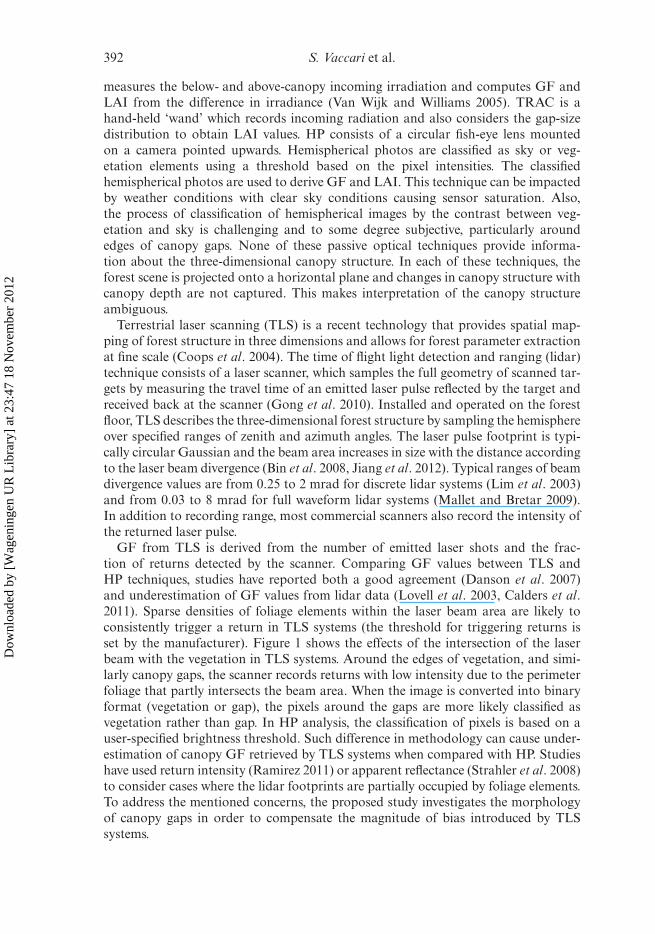
measures the below- and above-canopy incoming irradiation and computes GF andLAI from the difference in irradiance (Van Wijk and Williams 2005). TRAC is ahand-held ‘wand’ which records incoming radiation and also considers the gap-sizedistribution to obtain LAI values. HP consists of a circular fish-eye lens mountedon a camera pointed upwards. Hemispherical photos are classified as sky or veg-etation elements using a threshold based on the pixel intensities. The classifiedhemispherical photos are used to derive GF and LAI. This technique can be impactedby weather conditions with clear sky conditions causing sensor saturation. Also,the process of classification of hemispherical images by the contrast between veg-etation and sky is challenging and to some degree subjective, particularly aroundedges of canopy gaps. None of these passive optical techniques provide informa-tion about the three-dimensional canopy structure. In each of these techniques, theforest scene is projected onto a horizontal plane and changes in canopy structure withcanopy depth are not captured. This makes interpretation of the canopy structureambiguous.

Terrestrial laser scanning (TLS) is a recent technology that provides spatial map-ping of forest structure in three dimensions and allows for forest parameter extractionat fine scale (Coops et al. 2004). The time of flight light detection and ranging (lidar)technique consists of a laser scanner, which samples the full geometry of scanned tar-gets by measuring the travel time of an emitted laser pulse reflected by the target andreceived back at the scanner (Gong et al. 2010). Installed and operated on the forestfloor, TLS describes the three-dimensional forest structure by sampling the hemisphereover specified ranges of zenith and azimuth angles. The laser pulse footprint is typi-cally circular Gaussian and the beam area increases in size with the distance accordingto the laser beam divergence (Bin et al. 2008, Jiang et al. 2012). Typical ranges of beamdivergence values are from 0.25 to 2 mrad for discrete lidar systems (Lim et al. 2003)and from 0.03 to 8 mrad for full waveform lidar systems (Mallet and Bretar 2009).In addition to recording range, most commercial scanners also record the intensity ofthe returned laser pulse.

GF from TLS is derived from the number of emitted laser shots and the frac-tion of returns detected by the scanner. Comparing GF values between TLS andHP techniques, studies have reported both a good agreement (Danson et al. 2007)and underestimation of GF values from lidar data (Lovell et al. 2003, Calders et al.2011). Sparse densities of foliage elements within the laser beam area are likely toconsistently trigger a return in TLS systems (the threshold for triggering returns isset by the manufacturer). Figure 1 shows the effects of the intersection of the laserbeam with the vegetation in TLS systems. Around the edges of vegetation, and simi-larly canopy gaps, the scanner records returns with low intensity due to the perimeterfoliage that partly intersects the beam area. When the image is converted into binaryformat (vegetation or gap), the pixels around the gaps are more likely classified asvegetation rather than gap. In HP analysis, the classification of pixels is based on auser-specified brightness threshold. Such difference in methodology can cause under-estimation of canopy GF retrieved by TLS systems when compared with HP. Studieshave used return intensity (Ramirez 2011) or apparent reflectance (Strahler et al. 2008)to consider cases where the lidar footprints are partially occupied by foliage elements.To address the mentioned concerns, the proposed study investigates the morphologyof canopy gaps in order to compensate the magnitude of bias introduced by TLSsystems.

Dow

nloa

ded

by [

Wag

enin

gen

UR

Lib

rary

] at

23:

47 1

8 N

ovem

ber

2012

Bias in lidar-based canopy gap fraction estimates 393

Figure 1. TLS panoramic image (a) showing intensity values in terms of reflectance. Bluecolour represents absence of signal return and red colour represents high value of reflectance.Tree stems therefore tend to be displayed in red. (b) Zoomed-in tile of 1(a). Around each stema line of pixels with lower intensity (i.e. colour range between blue and red) is visible, denotinga situation in which part of the laser beam is reflected by vegetative material. When the imageis converted into binary format (i.e. distinguishing between canopy gap and vegetation), suchpixels are more likely classified as ‘vegetation’ rather than ‘gap’, leading to underestiomation ofGF. This pattern is repeated for the whole scene and for each scan.

2. Methods

2.1 Study area, instrument settings and data acquisition

The study area is located near the Loobos forest (De Hoge Veluwe National Park, theNetherlands) flux tower site. The forest is dominated by Scots Pine (Pinus sylvestris)with a sparse understory. Four homogeneous plots of 50 m × 50 m with varying treedensity (table 1) were established, and TLS and HP data were collected in September2011. Each plot was sampled at nine locations using a 25 m × 25 m regular squaresampling pattern.

Terrestrial lidar data were collected with an RIEGL VZ-400 terrestrial laser scanner(RIEGL Laser Measurement Systems GmbH, Horn, Austria, www.riegl.com), witha zenith and azimuth resolution of 1.05 mrad and beam divergence of 0.3 mrad.

Table 1. Statistical results per plot, sorted in order of tree density. For each of the three columns(Original, WP model correction and BP model correction), the statistics R2 and STD valueswere computed by averaging each of the nine scans in a plot. In the Original column, RMSEdescribes the original residual between GF values. In the WP and BP model correction columns,

the PRESSR statistic describes the residuals after the model correction.

Original WP model correction BP model correction

Plot

Tree density(no. perhectare) RMSE R2 STD PRESSR R2 STD PRESSR R2 STD

4 347 0.10 0.83 0.07 0.07 0.86 0.06 0.13 0.86 0.082 662 0.16 0.75 0.12 0.07 0.84 0.06 0.07 0.85 0.061 811 0.16 0.77 0.08 0.07 0.84 0.06 0.07 0.85 0.063 971 0.21 0.66 0.12 0.06 0.85 0.05 0.12 0.85 0.05

Dow

nloa

ded

by [

Wag

enin

gen

UR

Lib

rary

] at

23:

47 1

8 N

ovem

ber

2012

394 S. Vaccari et al.

Hemispherical photographs were made with a Nikon Coolpix 8700 camera, fitted withan FC-E9 Fisheye lens (180◦ field of view, Nikon, http://nikon.com/products/index.htm). The hemispherical camera was levelled horizontally using a bubble water leveland the scanner was visually levelled horizontally. For both instruments, GF analysiswas performed at full azimuth and at the zenith angle ranging from 30◦ to 90◦. Thezenith range was then divided into 120 zenith rings of 0.5◦ width. GF values werecomputed for each zenith ring.

2.2 Data analysis

The VZ-400 laser scanner records up to four returns per emitted laser beam. Onlyfirst returns are used for GF analysis in this study. The lidar dataset was projectedonto a panoramic coordinate frame and subsequently projected onto a polar projec-tion, in such a way, it could be compared against hemispherical photographs. In thiscase, azimuth and zenith resolutions were set slightly coarser (1.4 mrad) than the scanresolution settings (1.05 mrad), in order to ensure each solid angle of the hemispherescanned corresponded to an image pixel and to avoid empty pixels due to aliasing.Each pixel of the TLS and HP hemispherical images is described with an azimuthand zenith coordinate. TLS and HP polar images were converted into binary formatbased on the classification of each image pixel. Each pixel of the TLS data were classi-fied into canopy gap and canopy material based on whether returns were registered forlaser emissions under the respective angles. To classify the hemispherical photographs,the software Gap Light Analyser (Millbrook, NY, USA; Frazer et al. 1999) was used.For both TLS and HP binary images, canopy material and canopy gaps were labelledas 1 and 0, respectively.

GF was computed as the ratio of the number of pixels classified as canopy gap (pgap)to the total number of pixels (ptot) for each zenith ring, defined by a specific theta angleinterval ϑ:

GF(ϑ) = pgap(ϑ)/ptot(ϑ) (1)

Residuals between TLS- and HP-derived GF values were calculated for every sam-pling location and every zenith ring individually. To study the explanatory power ofgap morphology on the observed residuals, the single measure canopy perimeter wasdefined by pixel count on the TLS binary images. Canopy perimeters were obtainedusing a binary erosion operation (Maragos 1989). Binary erosion is a morphologi-cal image processing technique (Newnham et al. 2012) that analyses an image with apre-defined structuring element. In our case, a 3 × 3 pixel square window was usedas structuring element. Pixels with a value of 1 (canopy pixels) were eroded (i.e. setto 0) if the central pixel had a value of 0 (canopy gap). Due to the small dimension ofthe structuring element, erosion only occurs around canopy gaps. By subtracting twoimages, canopy perimeters were extracted.

Residuals between original TLS- and HP-derived GF values were calculated andplotted against canopy perimeter. To examine the stability of the relationship betweenGF residuals and canopy perimeter, models were created within plots (WPs) andbetween plots (BPs). For analysis WPs, one scan was left out at a time and theremaining eight scans were used as training set to create the model. For analysisBPs, the relationship between the two variables was determined from three plots and

Dow

nloa

ded

by [

Wag

enin

gen

UR

Lib

rary

] at

23:

47 1

8 N

ovem

ber

2012

Bias in lidar-based canopy gap fraction estimates 395

corrections were applied to the fourth. GF values of the test scan were adjusted basedon equation 2:

GFTLScorr (ϑ) = (GF)TLSorig (ϑ) + mmodel × cperimeter(ϑ) + qmodel (2)

For each model, the relationship between GF residuals and canopy perimeters wasassessed in terms of linear regression. The coefficients of such regression line (i.e. slope(mmodel and intercept (qmodel)), together with canopy perimeter information (cperimeter),contributed to adjust the original GF values retrieved by TLS (GFTLSorig ), in thedirection ϑ.

Linear correlation between TLS and HP GF estimates was used to assess the modelefficiency. Model performance was evaluated by the calculation of the coefficient ofdetermination R2, the standard deviation (STD), the root mean square error (RMSE)and the RMSE of the predicted sum of squares (PRESSR; Kozan and Gokce 2009).PRESSR values are calculated similar to RMSE values, but after the correction modelhas been applied. Therefore, the comparison between RMSE and PRESSR is a reliableindication of the effects of the model. PRESSR values smaller than RMSE valuesdenote an improvement in TLS-derived GF estimation.

3. Results

Canopy perimeters were computed from the TLS binary images by applying mor-phological erosion and subsequently by counting the eroded pixels (figure 2). Whenplotting the regression lines of GF residuals against canopy perimeter during themodel-creation procedure (figure 3), higher correlation is seen in forested areas withhigh tree density (plot 3). By averaging the R2 values of the single lines per plot, theR2 averaged (hereafter referred to as R2) value can be obtained. In plot 3, the highestR2 value was observed (R2 = 0.76), which is the plot with highest tree density. In con-trast, very low correlation was observed in plot 4. Plot 1 and plot 2 showed similar

Figure 2. Morphology erosion operation effects to compute canopy perimeter on TLS binaryimages. (a) Polar representation of a TLS scan, colour coded by intensity. Canopy gaps areassociated with light blue in the figure. (b) Binary image of 2(a). Canopy gaps are coloured inlight blue and vegetation is represented in dark blue. Canopy perimeter (in yellow) has beenextracted by eroding canopy pixels around canopy gaps.

Dow

nloa

ded

by [

Wag

enin

gen

UR

Lib

rary

] at

23:

47 1

8 N

ovem

ber

2012

396 S. Vaccari et al.

Figure 3. Regression lines of original GF residuals between TLS and HP, plotted per scanagainst canopy perimeter. The average of R2 values of each regression line is also displayed.(a) Plot 1, (b) plot 2, (c) plot 3 and (d) plot 4. Each plot was sampled at nine different locationsfollowing a square grid of 25 m × 25 m. Scan 5 is the centre plot.

results (R2 = 0.40 and 0.43, respectively) due to homogeneity in tree density and plotmorphology.

The corrective model was applied to each scan at WP and BP scale to test the effectsof gap morphology consideration in retrieval of GF values from TLS and HP. Thescatter plots showing improvements of GF values estimation at WP and BP scale com-pared to original GF values are displayed in figure 4. Statistics of each scatter plotare reported in table 1. PRESSR values of WP analysis significantly decrease com-pared to original RMSE values. Extreme values of RMSE and PRESSR comparisonimprovements are observed for plot 3 (RMSE = 0.21 and PRESSR = 0.06) and forplot 4 (RMSE = 0.10 and PRESSR = 0.07). When the model was generated with BP

Figure 4. Original, WP- and BP-corrected gap fraction values in comparison with the 1:1 line.(a) Plot 1, (b) plot 2, (c) plot 3 and (d) plot 4. When compared with original data, correctedregression lines are consistently closer to the 1:1 line, especially those related to the WP approachdue to the homogeneity of data used to create the model.

Dow

nloa

ded

by [

Wag

enin

gen

UR

Lib

rary

] at

23:

47 1

8 N

ovem

ber

2012

Bias in lidar-based canopy gap fraction estimates 397

approach, PRESSR values improved for every plot except plot 4 (RMSE = 0.10 andPRESSR = 0.13). Likewise, the standard deviation consistently decreased after themodel was applied, except for BP approach in plot 4.

Additionally, also R2 values and slopes of the regression lines of the scatter plotsbetween TLS- and HP-derived GF (figure 4) confirm the hypothesis of adjusting TLS-derived GF values using gap morphology. R2 of corrected GF values increases up to28% with both models for plot 3, where the results are improved the most. The leastimprovement, due to initial best GF estimation, is in plot 4. Comparing the slopesof the regression lines, the WP model (in red) leads to regression lines closer to the1:1 line in all the four plots. With the BP model (in yellow), the adjusted regressionlines also improve by approaching the 1:1 line, but they do not match as well as in WPmodel cases.

4. Discussion

The bias introduced by lidar in retrieving GF at the edges of canopy perimetershas major effect in dense forest canopies compared to open areas. This explains theregression lines of GF residuals plotted against canopy perimeter (figure 3), whichshow the highest and the lowest correlation in plot 3 and plot 4 (i.e. high and low den-sity forest), respectively. The bias effect is also indicated by the RMSE (table 1), whichis computed between original GF values estimated by TLS and HP. Low RMSE valuesindicate low difference between GF values retrieved by the two techniques. In contrast,a high RMSE is registered in high density forest, where the original difference of GFvalues is bigger due to the bias (plot 3). PRESSR values approach zero at both WPand BP scales, for all the plots except for plot 4, and are lower than RMSE values. Thisdenotes successful results of the model because it alleviates the original GF residualsbetween the two techniques. An improvement has not been achieved in plot 4 (in BPanalysis), because in this case, the model was created with plots which GF residualswere bigger (i.e. plot 1, plot 2 and plot 3) than those registered in plot 4 itself. Thus,the correction has negatively influenced the GF estimation. In figure 4, the model per-formances in WP and BP approaches are compared with original data. Both modelshad more influence where the original GF residuals were bigger (e.g. plot 3). In thiscase, R2 improved up to 28% (table 1).

Summarizing, the best improvements have been achieved in plot 3 due to the majoradjustment effect of the model in cases of dense canopies. In contrast, in cases of opencanopy structure (i.e. plot 4), TLS-derived GF is already well estimated and has agood agreement with HP (R2 = 0.83). This was observed as well by Danson et al.2007, who found a good fit between GF values estimated by TLS and HP withoutapplying any correctional methods. Future studies should investigate a potential treedensity threshold, above which the model is suggested to be applied and below whichthe TLS-derived GF values already reliably match the GF values obtained from HP.To further improve GF estimates from TLS, the analysis of gap morphology presentedherein may be combined with the use of return intensity (Ramirez 2011) to improveon the distinction between foliage and canopy gaps and to provide for a sub-pixelassessment of foliage densities.

5. Conclusion

The retrieval of canopy GF from TLS data is biased by sensitivity of the lidar instru-ment to record hits rather than gaps. This study investigates the distribution and

Dow

nloa

ded

by [

Wag

enin

gen

UR

Lib

rary

] at

23:

47 1

8 N

ovem

ber

2012

398 S. Vaccari et al.

length of the canopy perimeters that delineates the boundary between canopy gapsand foliage and uses length to correct biases in GF estimates. In dense forest canopies,the correction model presented herein improves estimates up to 28% compared to HP.In more open canopies, where canopy perimeters are generally shorter, improvementsin GF estimation are smaller.

AcknowledgementsThe authors acknowledge the Wageningen University Environmental ScienceDepartment and the Geo-information Science and Remote Sensing chair group fortheir support and the acquisition and processing of the terrestrial lidar data. Theauthors also thank Philip Wenting, Steisianasari Mileiva and Roberto Chávez for theircontribution during the data collection in September 2011. They also acknowledge thereviewers for their constructive feedback on the manuscript review.

ReferencesBIN, X., FANGFEI, L., KESHU, Z. and ZONGJIAN, L., 2008, Laser footprint size and

pointing precision analysis for LiDAR systems. The International Archives of thePhotogrammetry, Remote Sensing and Spatial Information Sciences, 37, pp. 331–336.

CALDERS, K., VERBESSELT, J., BARTHOLOMEUS, H. and HEROLD, M., 2011, Applying terrestrialLiDAR to derive gap fraction distribution time series during bud break. In Proceedingsof SilviLaser 2011, 11th International LiDAR Forest Applications Conference, 16–20October 2011, Hobart, Tasmania.

COOPS, N.C., WULDER, M.A., CULVENOR, D.S. and ST-ONGE, B., 2004, Comparison of for-est attributes extracted from fine spatial resolution multispectral and LiDAR data.Canadian Journal of Remote Sensing, 30, pp. 855–866.

DANSON, F.M., HETHERINGTON, D., MORSDORF, F., KOETZ, B. and ALLGÖWER, B., 2007,Forest canopy gap fraction from terrestrial laser scanning. IEEE Geoscience and RemoteSensing Letters, 4, pp. 157–160.

DEMAREZ, V., DUTHOIT, S., BARET, F., WEISS, M. and DEDIEU, G., 2008, Estimation of leafarea and clumping indexes of crops with hemispherical photographs. Agricultural andForest Meteorology, 148, pp. 644–655.

FRAZER, G.W., CANHAM, C.D. and LERTZMAN, K.P., 1999, Gap Light Analyser (GLA),Version 2.0: Imaging software to extract canopy structure and gap light transmissionindices from true-color fisheye photographs. Users manual and program documen-tation. Version 2.0. Copyright ©1999: Simon Fraser University, Burnaby, BritishColumbia, and the Institute of Ecosystem Studies, Millbrook, New York.

GONG, X., WEI, D. and ZHOU, G., 2010, Extracting trees and structure parameters via inte-gration of LiDAR data and ground imagery. In International Geoscience and RemoteSensing Symposium (IGARSS), Honolulu, HI, pp. 2703–2706.

GUEVARA-ESCOBAR, A., TELLEZ, J. and GONZALEZ-SOSA, E., 2005, Use of digital photographyfor analysis of canopy closure. Agroforestry Systems, 65, pp. 175–185.

JIANG, L.F., LAN, T., GU, M.X. and NI, G.Q., 2012, Effects of laser beam divergence angle onairborne LIDAR positioning errors. Journal of Beijing Institute of Technology (EnglishEdition), 21, pp. 278–284.

JONCKHEERE, I., FLECK, S., NACKAERTS, K., MUYS, B., COPPIN, P., WEISS, M. and BARET, F.,2004, Review of methods for in situ leaf area index determination Part I. Theories,sensors and hemispherical photography. Agricultural and Forest Meteorology, 121,pp. 19–35.

JONCKHEERE, I., NACKAERTS, K., MUYS, B. and COPPIN, P., 2005, Assessment of automaticgap fraction estimation of forests from digital hemispherical photography. Agriculturaland Forest Meteorology, 132, pp. 96–114.

Dow

nloa

ded

by [

Wag

enin

gen

UR

Lib

rary

] at

23:

47 1

8 N

ovem

ber

2012

Bias in lidar-based canopy gap fraction estimates 399

KOZAN, R. and GOKCE, M., 2009, Two-stage engine mapping for the calibration of carbonmonoxide emission. Modern Applied Science, 3, pp. 30–36.

LEBLANC, S.G., 2002, Correction to the plant canopy gap-size analysis theory used bythe tracing radiation and architecture of canopies instrument. Applied Optics, 41,pp. 7667–7670.

LEBLANC, S.G., CHEN, J.M., FERNANDES, R., DEERING, D.W. and CONLEY, A., 2005,Methodology comparison for canopy structure parameters extraction from digitalhemispherical photography in boreal forests. Agricultural and Forest Meteorology, 129,pp. 187–207.

LI-COR, 1992, LAI-2000 Plant Canopy Analyzer. Operating Manual (Lincoln, NE: LI-COR).LIM, K., TREITZ, P., WULDER, M., ST-ONGÉ, B. and FLOOD, M., 2003, LiDAR remote sensing

of forest structure. Progress in Physical Geography, 27, pp. 88–106.LOVELL, J.L., JUPP, D.L.B., CULVENOR, D.S. and COOPS, N.C., 2003, Using airborne and

ground-based ranging LiDAR to measure canopy structure in Australian forests.Canadian Journal of Remote Sensing, 29, pp. 607–622.

MALLET, C. and BRETAR, F., 2009, Full-waveform topographic LiDAR: state-of-the-art.ISPRS Journal of Photogrammetry and Remote Sensing, 64, pp. 1–16.

MARAGOS, P., 1989, A representation theory for morphological image and signal processing.IEEE Transactions on Pattern Analysis and Machine Intelligence, 11, pp. 586–599.

MARTENS, S.N., USTIN, S.L. and ROUSSEAU, R.A., 1993, Estimation of tree canopy leaf areaindex by gap fraction analysis. Forest Ecology and Management, 61, pp. 91–108.

NEWNHAM, G.J., SIGGINS, A.S., BLANCHI, R.M., CULVENOR, D.S., LEONARD, J.E. andMASHFORD, J.S., 2012, Exploiting three dimensional vegetation structure to mapwildland extent. Remote Sensing of Environment, 123, pp. 155–162.

RAMIREZ, F.A., 2011, Terrestrial laser scanning measurements to characterize temporalchanges in forest canopies. Unpublished PhD thesis, University of Salford, UK.

STRAHLER, A.H., JUPP, D.L.B., WOODCOCK, C.E., SCHAAF, C.B., YAO, T., ZHAO, F., YANG, X.,LOVELL, J., CULVENOR, D., NEWNHAM, G., NI-MIESTER, W. and BOYKIN-MORRIS, W.,2008, Retrieval of forest structural parameters using a ground-based LiDAR instrument(Echidna®). Canadian Journal of Remote Sensing, 34, pp. S426–S440.

VAN WIJK, M.T. and WILLIAMS, M., 2005, Optical instruments for measuring leaf areaindex in low vegetation: application in arctic ecosystems. Ecological Applications, 15,pp. 1462–1470.

VISSCHER VON, A.A., HUBER, S., KNEUBÜHLER, M. and ITTEN, K. 2007. Leaf area index esti-mates obtained for mixed forest using hemispherical photography and HYMAP data.In Proceedings of 10th ISPMSRS, 12–14 March 2007 (Davos, Switzerland: RemoteSensing Laboratories).

WARING, R.H. and RUNNING, S.W., 2007, Forest Ecosystems: Analysis at Multiple Scales,3rd ed. (Amsterdam: Elsevier).

WARREN, W.J., 1960, Analysis of the spatial distribution of foliage by two-dimensional pointquadrats. New Phytologist, 58, pp. 92–99.

Dow

nloa

ded

by [

Wag

enin

gen

UR

Lib

rary

] at

23:

47 1

8 N

ovem

ber

2012