SilviLaser 2011, Oct. 16-20, 2011 – Hobart, Australia

1

Applying terrestrial LiDAR to derive gap fraction distribution time series during bud break

Kim Calders1, Jan Verbesselt1, Harm Bartholomeus1 & Martin Herold1

1Laboratory of Geo-Information Science and Remote Sensing, Wageningen University, P.O. box 47, 6700 AA Wageningen (NL); kim.calders@wur.nl

Abstract The scientific community is witnessing a significant increase in the availability of different global satellite derived biophysical data sets. However, the use of such data is currently not supported by accurate in-situ biophysical measurement (e.g. canopy structure) in both a research and operational context for the monitoring of forest and land dynamics. Consequently, there is an urgent need for methods to measure in-situ canopy structure accurately and better integrate with improved and innovative remote sensing approaches. This paper explores the use of a ground-based, upward looking LiDAR instrument, combined with a fully automated analysis method to retrieve the gap fraction distribution. Traditional inventory methods for the assessment of forest structure are less objective or based on a 2D approach. We compare the seasonal dynamics of gap fraction distribution from hemispherical photographs and terrestrial LiDAR measurement during bud break. Preliminary analysis shows that gap fraction distributions derived from terrestrial LiDAR were consistently lower than the values obtained from hemispherical photography. This might indicate that the LiDAR scans at the centre position of the plot are not representing the plot scale variation. However, the LiDAR based methodology is fully automated, requires no operator interference and is more objective, whereas the analysis of hemispherical photographs requires a large number of operator decisions (e.g. thresholding). Further improvements of this LiDAR-based method can still be achieved by (i) a better understanding of scanner settings and data resolution on the derived gap fraction and (ii) integration of target intensity in the analysis. This paper highlighted the high potential and need for a robust method to derive gap fraction distributions to monitor seasonal dynamics in forests. Keywords: Terrestrial LiDAR, forestry, canopy structure, gap fraction, seasonal dynamics 1. Introduction Forested areas play an important role in today’s society and serve as a source for the production of paper products, lumber and fuel wood. In addition, forests produce freshwater from mountain watersheds, purify the air, offer habitat to wildlife and offer recreational opportunities. To keep these production, ecological and recreational functions balanced, accurate and precise information about forest structure and its biophysical parameters is needed (Warning & Running, 2007). Forest structure closely relates to several biological and physical processes. For example, respiration, transpiration, photosynthesis, carbon and nutrient cycle and rainfall interception heavily depend on the structural arrangement within the forest. Additionally, the terrestrial biosphere acts as a large sink for carbon dioxide (CO2). In times where global warming is an important issue, accurate and precise measurements of forest variables are needed for the observations of Essential Climate Variables (ECVs) and for reducing emissions from deforestation and forest degradation (REDD). Remote sensing methods are useful tools to obtain this structural and biophysical information and they can be applied over extensive and inaccessible areas.

SilviLaser 2011, Oct. 16-20, 2011 – Hobart, Australia

2

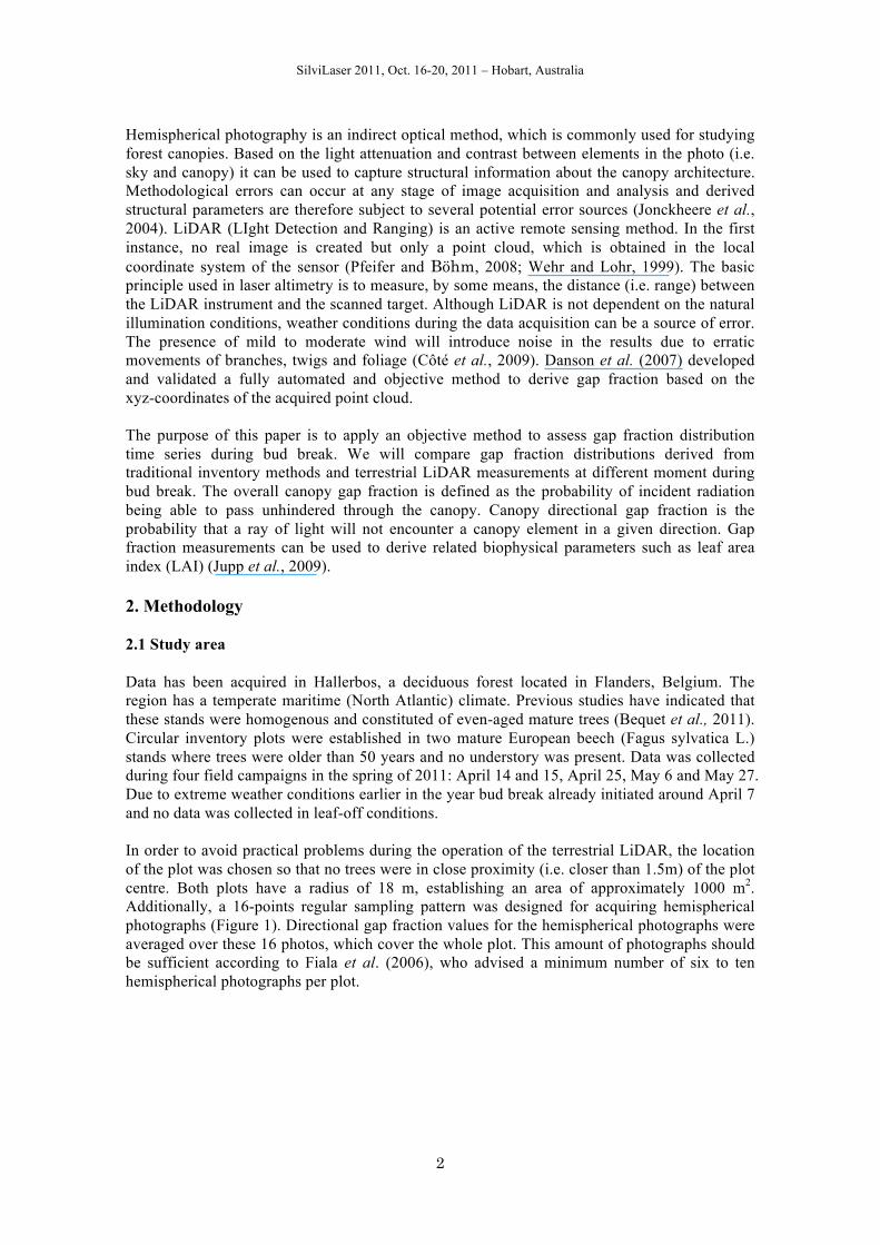
Hemispherical photography is an indirect optical method, which is commonly used for studying forest canopies. Based on the light attenuation and contrast between elements in the photo (i.e. sky and canopy) it can be used to capture structural information about the canopy architecture. Methodological errors can occur at any stage of image acquisition and analysis and derived structural parameters are therefore subject to several potential error sources (Jonckheere et al., 2004). LiDAR (LIght Detection and Ranging) is an active remote sensing method. In the first instance, no real image is created but only a point cloud, which is obtained in the local coordinate system of the sensor (Pfeifer and Böhm, 2008; Wehr and Lohr, 1999). The basic principle used in laser altimetry is to measure, by some means, the distance (i.e. range) between the LiDAR instrument and the scanned target. Although LiDAR is not dependent on the natural illumination conditions, weather conditions during the data acquisition can be a source of error. The presence of mild to moderate wind will introduce noise in the results due to erratic movements of branches, twigs and foliage (Côté et al., 2009). Danson et al. (2007) developed and validated a fully automated and objective method to derive gap fraction based on the xyz-coordinates of the acquired point cloud. The purpose of this paper is to apply an objective method to assess gap fraction distribution time series during bud break. We will compare gap fraction distributions derived from traditional inventory methods and terrestrial LiDAR measurements at different moment during bud break. The overall canopy gap fraction is defined as the probability of incident radiation being able to pass unhindered through the canopy. Canopy directional gap fraction is the probability that a ray of light will not encounter a canopy element in a given direction. Gap fraction measurements can be used to derive related biophysical parameters such as leaf area index (LAI) (Jupp et al., 2009). 2. Methodology 2.1 Study area Data has been acquired in Hallerbos, a deciduous forest located in Flanders, Belgium. The region has a temperate maritime (North Atlantic) climate. Previous studies have indicated that these stands were homogenous and constituted of even-aged mature trees (Bequet et al., 2011). Circular inventory plots were established in two mature European beech (Fagus sylvatica L.) stands where trees were older than 50 years and no understory was present. Data was collected during four field campaigns in the spring of 2011: April 14 and 15, April 25, May 6 and May 27. Due to extreme weather conditions earlier in the year bud break already initiated around April 7 and no data was collected in leaf-off conditions. In order to avoid practical problems during the operation of the terrestrial LiDAR, the location of the plot was chosen so that no trees were in close proximity (i.e. closer than 1.5m) of the plot centre. Both plots have a radius of 18 m, establishing an area of approximately 1000 m2. Additionally, a 16-points regular sampling pattern was designed for acquiring hemispherical photographs (Figure 1). Directional gap fraction values for the hemispherical photographs were averaged over these 16 photos, which cover the whole plot. This amount of photographs should be sufficient according to Fiala et al. (2006), who advised a minimum number of six to ten hemispherical photographs per plot.

SilviLaser 2011, Oct. 16-20, 2011 – Hobart, Australia

3

Figure 1: Schematic plot overview. LiDAR measurements were performed at location X using 2 different configurations. Hemispherical photographs were taken at each location on the 16-points regular grid. 2.2 Hemispherical photography In this study a Nikon Coolpix 8700 (8 megapixels) fitted with an FC-E9 Fisheye lens (180 degrees field of view) was used. The camera was fixed on a pole and the position of the lens was levelled in the horizontal and vertical direction using a water level. The top of the lens was pointed towards the sky and located at 1.3 m above the ground surface. Pictures were taken at the highest resolution and quality with a fixed ISO at 200. Weather conditions during the different field campaigns varied but in general the photographs were taken in overcast sky conditions. For the processing of the hemispherical photographs, the Hemisfer software (Swiss Federal Institute for Forest, Snow and Landscape Research WSL) was used (Schleppi et al., 2007). Only the blue channel of the image was chosen to be included in the analysis since it gives the maximum contrast between leaf and sky (Zhao et al., 2011) and the lens parameters were set to match those of the Nikon FC-E9. Thresholding is a crucial step in processing the hemispherical photos, which affects all further calculations. Manual thresholding is a subjective task and hard to reproduce consistently. A comparison study by Jonckheere et al. (2005) found that the method of Ridler & Calvard (1978) was most optimal and robust for a wide range of light and canopy structure conditions. Therefore this clustering-based automatic threshold method was applied to classify the pixels either as black (canopy) or as white (sky). This method was based on finding the midpoint between two clusters by iteratively estimating the average of two cluster means. The hemisphere was divided in 18 rings of 5 degrees and the directional gap fraction for each of those zenith rings was calculated. In the first step, gap fraction was derived within the defined rings based on the number of black and white pixels. These values were then corrected for non-linearity within the rings and ground slope (Schleppi et al., 2007). Results were calculated for the weighted means of all zenith angles within a ring since there are more pixels along the outer border of a ring than along the inner border. 2.3 LiDAR measurements The RIEGL VZ-400 3D terrestrial laser scanner was used to acquire terrestrial LiDAR data in the study area. This type of scanner uses a line scanning mechanism that is based upon a fast rotating multi-facet polygonal mirror. This leads to fully linear, unidirectional and parallel scan lines. The instruments operates in the infrared (1550 nm) and has a range up to 600 m. Due to

SilviLaser 2011, Oct. 16-20, 2011 – Hobart, Australia

4

the on-board online waveform processing, the scanner is able to record multiple target echoes (RIEGL laser measurement systems, 2011). LiDAR data was acquired at the centre location of the plot (Figure 1). The scanner was mounted on a tripod and tilted 90°. At the scan position two orthogonal scans were made. We consistently orientated the scanner so that the hemisphere was scanned in the East-West-direction by the first scan and the North-South-direction by the second scan. The frame scan angle was set to 180° (i.e. the upper hemisphere) and the line scan angle to 100°. Both frame and line resolutions were 0.04° (Table 1).

Table 1: RIEGL VZ-400 settings for the data acquisition

Frame scan angle 180°

Line scan angle 100°

Frame resolution 0.04°

Line resolution 0.04°

Inclination angle 90°

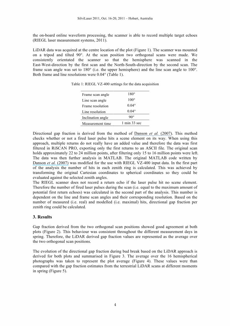
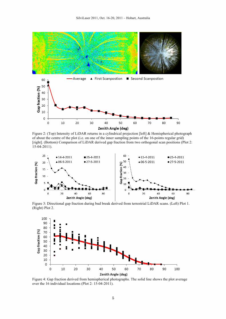
Measurement time 1 min 33 sec Directional gap fraction is derived from the method of Danson et al. (2007). This method checks whether or not a fired laser pulse hits a scene element on its way. When using this approach, multiple returns do not really have an added value and therefore the data was first filtered in RiSCAN PRO, exporting only the first returns to an ASCII file. The original scan holds approximately 22 to 24 million points, after filtering only 15 to 16 million points were left. The data was then further analysis in MATLAB. The original MATLAB code written by Danson et al. (2007) was modified for the use with RIEGL VZ-400 input data. In the first part of the analysis the number of hits in each zenith ring is calculated. This was achieved by transforming the original Cartesian coordinates to spherical coordinates so they could be evaluated against the selected zenith angles. The RIEGL scanner does not record a return echo if the laser pulse hit no scene element. Therefore the number of fired laser pulses during the scan (i.e. equal to the maximum amount of potential first return echoes) was calculated in the second part of the analysis. This number is dependent on the line and frame scan angles and their corresponding resolution. Based on the number of measured (i.e. real) and modelled (i.e. maximal) hits, directional gap fraction per zenith ring could be calculated. 3. Results Gap fraction derived from the two orthogonal scan positions showed good agreement at both plots (Figure 2). This behaviour was consistent throughout the different measurement days in spring. Therefore, the LiDAR derived gap fraction values are represented as the average over the two orthogonal scan positions. The evolution of the directional gap fraction during bud break based on the LiDAR approach is derived for both plots and summarised in Figure 3. The average over the 16 hemispherical photographs was taken to represent the plot average (Figure 4). These values were than compared with the gap fraction estimates from the terrestrial LiDAR scans at different moments in spring (Figure 5).

SilviLaser 2011, Oct. 16-20, 2011 – Hobart, Australia

5

Figure 2: (Top) Intensity of LiDAR returns in a cylindrical projection [left] & Hemispherical photograph of about the centre of the plot (i.e. on one of the inner sampling points of the 16-points regular grid) [right]. (Bottom) Comparison of LiDAR derived gap fraction from two orthogonal scan positions (Plot 2: 15-04-2011).

Figure 3: Directional gap fraction during bud break derived from terrestrial LiDAR scans. (Left) Plot 1. (Right) Plot 2.

Figure 4: Gap fraction derived from hemispherical photographs. The solid line shows the plot average over the 16 individual locations (Plot 2: 15-04-2011).

SilviLaser 2011, Oct. 16-20, 2011 – Hobart, Australia

6

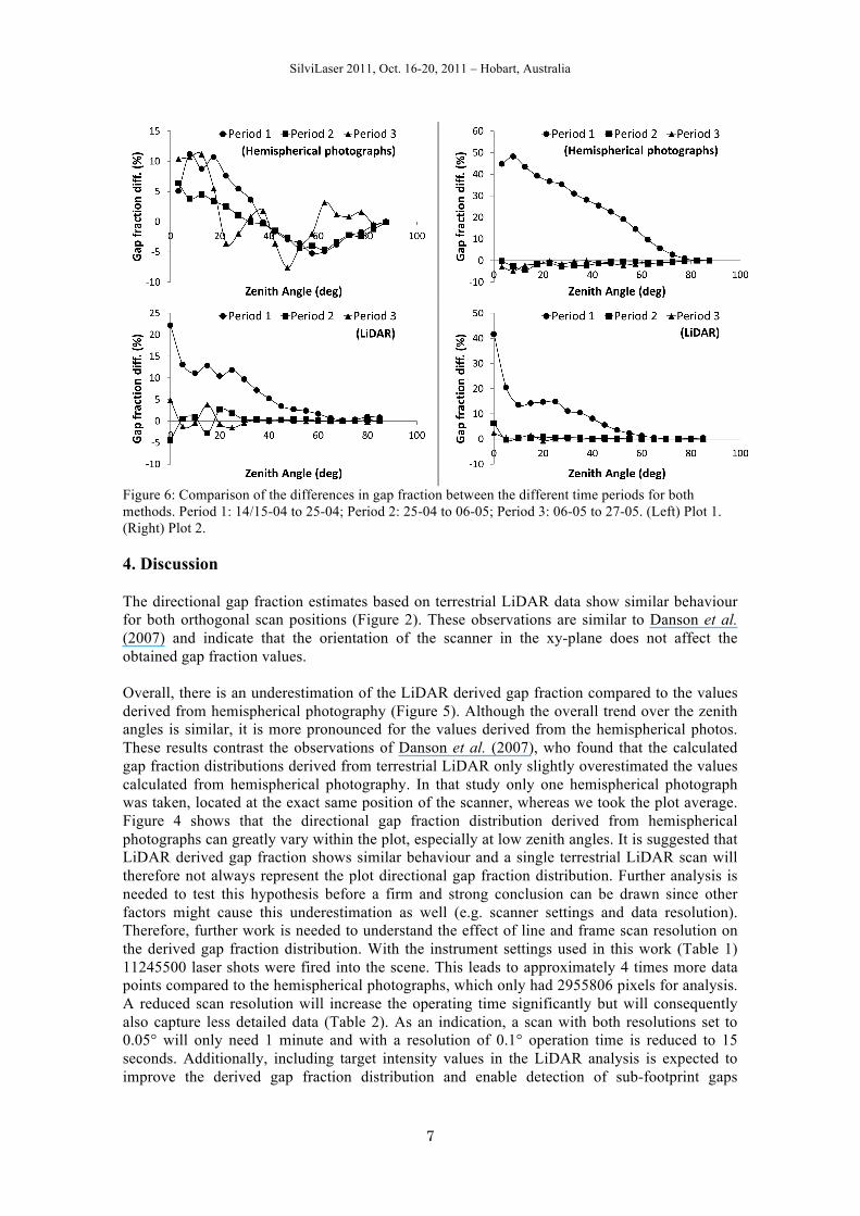
Finally, the relative differences between the four points in time were calculated for both methods (Figure 6). Period 1 represent the changes in gap fraction distribution between April 14/15 and April 25, period 2 represents the changes between April 25 and May 6 and the third period represents the changes between May 6 and May 27. Values from the later date are subtracted from the earlier date.

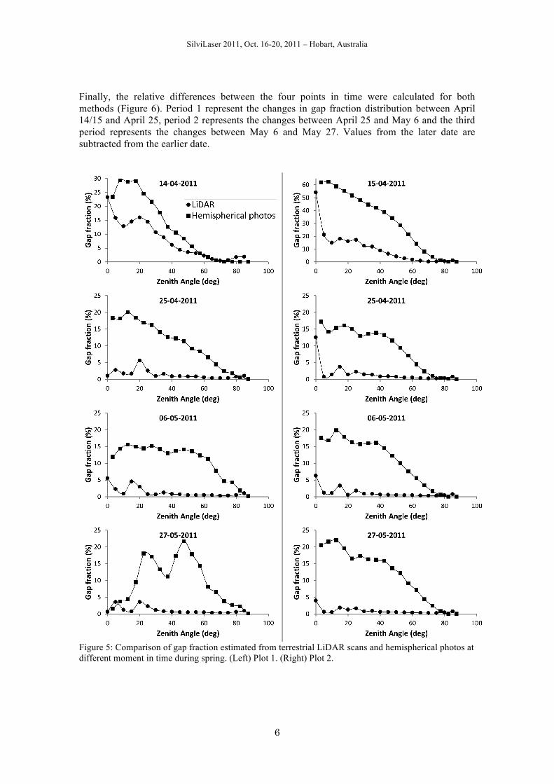
Figure 5: Comparison of gap fraction estimated from terrestrial LiDAR scans and hemispherical photos at different moment in time during spring. (Left) Plot 1. (Right) Plot 2.

SilviLaser 2011, Oct. 16-20, 2011 – Hobart, Australia

7

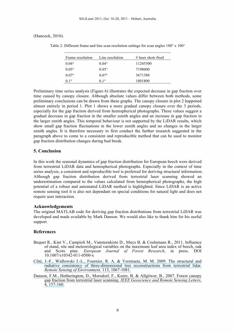
Figure 6: Comparison of the differences in gap fraction between the different time periods for both methods. Period 1: 14/15-04 to 25-04; Period 2: 25-04 to 06-05; Period 3: 06-05 to 27-05. (Left) Plot 1. (Right) Plot 2. 4. Discussion The directional gap fraction estimates based on terrestrial LiDAR data show similar behaviour for both orthogonal scan positions (Figure 2). These observations are similar to Danson et al. (2007) and indicate that the orientation of the scanner in the xy-plane does not affect the obtained gap fraction values. Overall, there is an underestimation of the LiDAR derived gap fraction compared to the values derived from hemispherical photography (Figure 5). Although the overall trend over the zenith angles is similar, it is more pronounced for the values derived from the hemispherical photos. These results contrast the observations of Danson et al. (2007), who found that the calculated gap fraction distributions derived from terrestrial LiDAR only slightly overestimated the values calculated from hemispherical photography. In that study only one hemispherical photograph was taken, located at the exact same position of the scanner, whereas we took the plot average. Figure 4 shows that the directional gap fraction distribution derived from hemispherical photographs can greatly vary within the plot, especially at low zenith angles. It is suggested that LiDAR derived gap fraction shows similar behaviour and a single terrestrial LiDAR scan will therefore not always represent the plot directional gap fraction distribution. Further analysis is needed to test this hypothesis before a firm and strong conclusion can be drawn since other factors might cause this underestimation as well (e.g. scanner settings and data resolution). Therefore, further work is needed to understand the effect of line and frame scan resolution on the derived gap fraction distribution. With the instrument settings used in this work (Table 1) 11245500 laser shots were fired into the scene. This leads to approximately 4 times more data points compared to the hemispherical photographs, which only had 2955806 pixels for analysis. A reduced scan resolution will increase the operating time significantly but will consequently also capture less detailed data (Table 2). As an indication, a scan with both resolutions set to 0.05° will only need 1 minute and with a resolution of 0.1° operation time is reduced to 15 seconds. Additionally, including target intensity values in the LiDAR analysis is expected to improve the derived gap fraction distribution and enable detection of sub-footprint gaps

SilviLaser 2011, Oct. 16-20, 2011 – Hobart, Australia

8

(Hancock, 2010).

Table 2: Different frame and line scan resolution settings for scan angles 180° x 100°

Frame resolution Line resolution # laser shots fired 0.04° 0.04° 11245500 0.05° 0.05° 7198000 0.07° 0.07° 3671388 0.1° 0.1° 1801800

Preliminary time series analysis (Figure 6) illustrates the expected decrease in gap fraction over time caused by canopy closure. Although absolute values differ between both methods, some preliminary conclusions can be drawn from these graphs. The canopy closure in plot 2 happened almost entirely in period 1. Plot 1 shows a more gradual canopy closure over the 3 periods, especially for the gap fraction derived from hemispherical photographs. These values suggest a gradual decrease in gap fraction in the smaller zenith angles and an increase in gap fraction in the larger zenith angles. This temporal behaviour is not supported by the LiDAR results, which show small gap fraction fluctuations in the lower zenith angles and no changes in the larger zenith angles. It is therefore necessary to first conduct the further research suggested in the paragraph above to come to a consistent and reproducible method that can be used to monitor gap fraction distribution changes during bud break. 5. Conclusion In this work the seasonal dynamics of gap fraction distribution for European beech were derived from terrestrial LiDAR data and hemispherical photographs. Especially in the context of time series analysis, a consistent and reproducible tool is preferred for deriving structural information. Although gap fraction distribution derived from terrestrial laser scanning showed an underestimation compared to the values calculated from hemispherical photographs, the high potential of a robust and automated LiDAR method is highlighted. Since LiDAR is an active remote sensing tool it is also not dependant on special conditions for natural light and does not require user interaction. Acknowledgements The original MATLAB code for deriving gap fraction distributions from terrestrial LiDAR was developed and made available by Mark Danson. We would also like to thank him for his useful support. References Bequet R., Kint V., Campioli M., Vansteenkiste D., Muys B. & Ceulemans R., 2011. Influence

of stand, site and meteorological variables on the maximum leaf area index of beech, oak and Scots pine. European Journal of Forest Research, in press. DOI 10.1007/s10342-011-0500-x

Côté, J.-F., Widlowski J.-L., Fournier, R. A. & Verstraete, M. M. 2009. The structural and radiative consistency of three-dimensional tree reconstructions from terrestrial lidar. Remote Sensing of Environment, 113, 1067-1081.

Danson, F.M., Hetherington, D., Morsdorf, F., Koetz, B. & Allgöwer, B., 2007. Forest canopy gap fraction from terrestrial laser scanning. IEEE Geoscience and Remote Sensing Letters, 4, 157-160.

SilviLaser 2011, Oct. 16-20, 2011 – Hobart, Australia

9

Fiala, A. C. S., Garman, S. L., & Gray, A. N., 2006. Comparison of five canopy cover estimation techniques in the western Oregon Cascades. Forest ecology and management, 232, 188-197.

Hancock, S., 2010. Understanding the measurement of forests with waveform lidar. PhD thesis, UCL Geography

Jonckheere, I., Nackaerts, K., Muys, B. & Coppin, P., 2005. Assessment of automatic gap fraction estimation of forests from digital hemispherical photography. Agricultural and Forest Meteorology, 132, 96-114.

Jonckheere, I., Fleck, S., Nackaerts, K., Muys, B., Coppin, P., Weiss, M. & Baret, F., 2004. Review of methods for in situ leaf area index determination Part I. Theories, sensors and hemispherical photography. Agricultural and Forest Meteorology, 121, 19-35.

Jupp, D.L.B., Culvenor, D.S., Lovell, J.L., Newnham, G.J., Strahler, A.H. & Woodcock, C.E., 2009. Estimating forest LAI profiles and structural parameters using a ground-based laser called Echidna®. Tree physiology, 29, 171-181.

Pfeifer, N. & Böhm, J., 2008. Early stages of LiDAR data processing. In Advances in photogrammetry, remote sensing and spatial information sciences: 2008 ISPRS congress book

Ridler W. & Calvard S., 1978. Picture thresholding using an iterative selection method. IEEE Trans. Syst. Man Cyber., 8, 260-263.

RIEGL laser measurement systems, 2011, www.riegl.com, accessed 4th June 2011 Schleppi P., Conedera M., Sedivy I., Thimonier A., 2007. Correcting non-linearity and slope

effects in the estimation of the leaf area index of forests from hemispherical photographs. Agric. Forest Meteorol., 144, 236–242.

Warning, R. H. & Running, S. W., 2007. Forest ecosystems analysis at multiple scales, 3rd edn, Elsevier, 420p.

Wehr, A., U. Lohr. 1999. Airborne laser scanning - An introduction and overview. ISPRS Journal of Photogrammetry and Remote Sensing, 54, 68-82.

Zhao, F., Yang, X., Schull, M.A., Román-Colón, M.O., Yao, T., Wang, Z., Zhang, Q., Jupp, D.L.B., Lovell, J.L., Culvenor, D.S., Newnham, G.J., Richardson, A.D., Ni-Meister, W., Schaaf, C.L., Woodcock, C.E. & Strahler, A.H., 2011. Measuring effective leaf area index, foliage profile, and stand height in New England forest stands using a full-waveform ground-based lidar. Remote Sensing of Environment, in press. DOI 10.1016/j.rse.2010.08.030