ORIGINAL PAPER

Grapevine bud break prediction for cool winter climates

Claas Nendel

Received: 15 June 2009 /Revised: 8 September 2009 /Accepted: 16 September 2009# ISB 2009

Abstract Statistical analysis of bud break data for grape-vine (Vitis vinifera L. cvs. Riesling and Müller-Thurgau) at13 sites along the northern boundary of commercial grape-vine production in Europe revealed that, for all investigatedsites, the heat summation method for bud break predictioncan be improved if the starting date for the accumulation ofheat units is specifically determined. Using the coefficientof variance as a criterion, a global minimum for each sitecan be identified, marking the optimum starting date. Fur-thermore, it was shown that the application of a thresholdtemperature for the heat summation method does not lead toan improved prediction of bud break. Using site-specificparameters, bud break of grapevine can be predicted withan accuracy of ± 2.5 days. Using average parameters, theprediction accuracy is reduced to ± 4.5 days, highlightingthe sensitivity of the heat summation method to the qualityand the representativeness of the driving temperature data.

Keywords Grapevine . Phenology .Modelling .

Heat unit accumulation

Introduction

Modelling crop growth of grapevine is a precondition forall dynamic simulations studies concerned with nutrient orwater cycling in vineyards or the impact of climate changeon wine production. One of the key processes to be under-stood is how phenology of the perennial crop is controlled.The different stages of development, beginning with bud

burst in spring, govern many processes related to thegrowth of different plant organs, the overall yield and thequality performance of the crop. Grapevine is neither sownnor transplanted at the beginning of the season, so asimulation model needs to be able to determine the start ofgrapevine development from available input data, such aslocal climate. Bud burst is calculated quite differently indifferent crop growth models available for grapevine (Bindiet al. 1997; Gutierrez et al. 1985; Nendel and Kersebaum2004; Wermelinger et al. 1991; Williams et al. 1985). How-ever, all approaches used are based on the heat accumula-tion method and are thus categorised as statistical models inthe sense referred to by Chuine et al. (2003). The heataccumulation method dates from early investigations as farback as the eighteenth century (de Réaumur 1735) and hasbeen used throughout the following centuries (Burckhardt1860; Magoon and Culpepper 1932). Lindsey and Newman(1956) first proposed a detailed methodology of the time–temperature concept after having worked out the temperatureinfluence on early or late flowering of different plants. Themethod was later tested against phenology data of JapaneseCherry (Prunus serrulata; Lindsey 1963). The concept wasrefined in many subsequent works (Abrami 1972; Allen1976; Arnold 1960; Baskerville and Emin 1969) andtransferred to other biological systems (e.g. Eckenrode andChapman 1972; Gilbert and Gutierrez 1973; Sevacherianet al. 1977).

The development of Vitis vinifera was found to bemainly temperature driven (Alleweldt 1960; Christiansen1969; May 1964; Peyer and Koblet 1966; Winkler 1962).However, the proposed methods for phenological date cal-culation still differ in many details: Besselat et al. (1995)and Alleweldt and Hofäcker (1975) accumulate dailymaximum temperatures; for flowering date forecast, Caloet al. (1994) found the sum of daily mean temperatures onlymarginally less successful than the sum of daily maximum

C. Nendel (*)Leibniz-Centre for Agricultural Landscape Research,Institute for Landscape System Analysis,Eberswalder Straße 84,15374 Müncheberg, Germanye-mail: nendel@zalf.de

Int J BiometeorolDOI 10.1007/s00484-009-0274-8

temperatures, while Peyer and Koblet (1966) suggest usingonly day temperatures above 15°C. Later, Pouget (1988)considered only the temperature range between 5 and 25°Cas valid for bud burst prediction. McIntyre et al. (1987)criticised the use of daily temperatures, since the intra-dailytemperature dynamics would also considerably influencethe process of bud burst.

However, above all it is the choice of threshold tem-perature and the starting date for heat unit accumulationthat is decisive for the predictive quality of statisticalmodels (Wielgolaski 1999). There is consensus regardingplant growth ceasing below a certain temperature threshold,for which reason Lindsey and Newman (1956) introduced aphysiological threshold temperature to their heat sum ap-proach. For grapevine, a threshold temperature of 8°C(Alleweldt and Hofäcker 1975) or 10°C (Buttrose and Hale1973; Horney 1966; Williams et al. 1985) is proposed.However, threshold temperatures for bud break calculationof many wood species in Northern Europe have been foundto be much lower, even below zero (Wielgolaski 1999).From growth studies with Vitis vinifera cultivars grown inAustralia, Moncur et al. (1989) suggested employingthreshold temperatures below 4°C. Lopes et al. (2008) used3.5°C for their study on bud break of Portuguese cultivars.

By calculative optimisation, Besselat et al. (1995) found1 January to be the optimum date to start heat unit accu-mulation, while Williams et al. (1985) found this date to be20 February. Horney (1966) went for 1 January in yearswithout frost. However, he made a crucial remark on thereversion of the vertical soil temperature gradient reallybeing the optimum starting date in spring (see also Hickinand Vittum 1976; Wolfart et al. 1988). Isothermy between50 and 100 cm soil depth practically coincides with the saprising in the vines in spring. At Geisenheim, Germany, thisdate fell on 17 March as the mean of the years 1946–1965(Horney 1966). Alleweldt and Hofäcker (1975) used 15March as their starting date; however, they did not justifytheir choice.

The present study was carried out to investigate whichthreshold temperature and which starting date for heat unitaccumulation for predictive bud-break simulation is opti-mum for northern European vineyards by using a simpleoptimisation procedure. The result serves a bud-breakprediction algorithm in state-of-the-art crop growth model-ling in viticulture.

Material and methods

Starting date for heat unit accumulation

To determine the optimum starting date for heat unit accu-mulation in degree-days, historical bud break data were

used with corresponding data on daily air temperatures. Forcalculation of degree-days, the single triangle algorithm(Zalom et al. 1983) was used.

D ¼0 for T0 � Tmax

Tmax�T02

� �Tmax�T0Tmax�Tmin

� �for Tmin < T0 < Tmax

Tm � T0 for T0 � Tmin

8<

:

ð1Þwith Tmax, Tm, Tmin being the daily maximum, mean, andminimum temperature and T0 being the threshold tem-perature for vine growth. The degree-days, D, were summeduntil the respective bud-break date, beginning with 1January. The resulting heat sum, H1, was compared to otheryears and the coefficient of variation (CV—the standarddeviation divided by the mean) was computed. Subsequent-ly, the starting date for heat summation was reduced by1 day, putting 2 January into starting position for calculatingH2. This iteration was conducted up until 31 March.

Hd ¼X90

i¼d

Dið Þ ð2Þ

with Hd being the heat sum for a specific starting date d(1 January = 1). The mean heat sum and standard deviationfor the respective number of years were calculated accord-ing to

Hd ¼Pa

i¼1Hdð Þa

ð3Þ

s Hdð Þ ¼ffiffiffiffiffiffiffiffiffiffiffiffiffiffiffiffiffiffiffiffiffiffiffiffiffiffiffiffiffiffiffiffiffiffiffiffiffiffiffiffiffiffiffiffiffiffiffiffi1

a� 1�Xa

i¼1

Hi;d � Hd

� �2s

ð4Þ

with a being the number of years considered.A calculation routine is given with a parameter vector

Φ = (d, T0). The criterion L(Φ) for the parameter estimationproblem is the CV, calculated by dividing the standarddeviation of the heat sum Hd for all years by the mean heatsum Hd for a specific starting date d.

L 6ð Þ ¼ s Hdð ÞHd

� �ð5Þ

The optimisation problem is to find a parameter vector Φsuch that

L 6̂� �

¼ minΦ2U

L 6ð Þ ð6Þ

where U denotes the admissible parameter space for Φ,which is d ∈ [1, 90] and T0 ∈ [0, 12°C] (see Fig. 1).

Int J Biometeorol

Threshold temperature for heat unit accumulation

To determine the threshold temperature to be used for heatunit accumulation, CV was calculated for threshold temper-atures T0 ranging from 0.0 to 12.0°C, beginning with heatunit accumulation at the optimum date found in the pre-vious procedure. Plotting CV against T0 yields a curve withan almost linear pattern at both ends. By fitting two linearmodels to the data points in the range T0,low = [0; 3°C] andT0,up = [7; 12°C] two lines are obtained, whose intersectionmarks the desired threshold temperature T0. This approachwas chosen in order to employ a mathematically sound androbust method for the determination of T0, as demonstratedfor data from Neustadt an der Weinstraße in Fig. 2.

Phenological and weather data

For this investigation, data sets of 13 vineyards in northernEurope were available: Bad Kreuznach (49°51′ N, 7°49′ E),Bernkastel-Kues (49°55′ N, 7°04′ E), Lahr (48°02′ N,7°38′ E), Neustadt an der Weinstraße (49°23′ N, 8°11′ E),Oppenheim (49°52′ N, 8°20′ E), Stuttgart-Schnarrenberg(48°49′ N, 9°12′ E), Trier (49°44′ N, 6°39′ E), Veitshöchheim(49°50′ N, 9°52′ E) and Weinsberg (49°09′ N, 9°17′ E) inGermany, Angers (47°07′ N, 0° 07′ E) in France, Dvory nadŽitavou (48°00′ N, 18°16′ E) in Slovakia, Velké Žernoseky(50°32′ N, 14°04′ E) in the Czech Republic and Remich(49°32′ N, 6°22′ E) in Luxemburg (Fig. 3). The grapevarieties considered are Riesling as a late-, and Müller-Thurgau as an early-developing variety. Phenology wasdescribed according to the Biologische Bundesanstalt,Bundessortenamt, Chemische Industrie (BBCH) scale, in

which crop development is classified in macro-stages(Lorenz et al. 1994). For grapevine, the stages are termedbud break, leaf development, emergence of inflorescences,bloom, fruit development, fruit maturity and dormancy. Sub-stages are used to further classify important indications ofphenological development. In this investigation bud breakwas determined according to the developmental stage BBCH09 (green tips clearly visible; Lorenz et al. 1994), alsodescribed as 50% of the shoots being 2 cm long. For Angers,Dvory nad Žitavou, Stuttgart-Schnarrenberg and VelkéŽernoseky, only BBCH 07 (green tips start to show; Lorenzet al. 1994) was available. For these sites, BBCH 09 wasassumed to occur on average 2 days later. Temperature datafor Trier have been adjusted to the lower altitude of thephenological station, which is located 88 m beneath theweather station at a distance of 600 m. A gradient of 0.65°Cper 100 m was applied for this purpose.

Data analysis revealed that, within the data sets, a fewyears significantly compromise the calculation of a low CV.Possible reasons for this effect are manifold and arediscussed below. In order to achieve a stable model, theseyears were excluded from the data set (see annotation inTable 1 for details).

Bud break date prediction

The mean accumulated heat sum for optimum prediction iscalled the degree-day target HT. The prediction algorithmsums up the degree-days D as calculated above (Eq. 1),starting from the determined optimum starting date dopt untilthe degree-day target HT is reached (Table 1). The degree-

Fig. 2 Coefficient of variation of accumulated daily mean temper-atures from 25 February (determined optimum starting date) untilgrapevine bud-break plotted against threshold temperatures atNeustadt an der Weinstraße. Two linear functions were fitted to the[0°C, 3°C] and [7°C, 12°C] intervals, respectively. The intersectionof these two lines marks the threshold temperature for the heatsummation algorithm

Fig. 1 Coefficient of variation (CV) of accumulated daily meantemperatures until grapevine bud break for different starting dates andthreshold temperatures at Neustadt an der Weinstraße, Germany

Int J Biometeorol

day target is adjusted on a daily basis by subtracting 0.5Dfrom HT to account for high values of D by far exceeding thetarget, and thus the predicted bud break date by 1 day.

Cross validation

A cross validation was carried out in order to test thepredictive quality of the model. Due to the small size of thedata set the leave-one-out method (Lachenbruch andMickey 1968) was used. Given the number of data sets n,the bud break dates of one data set were predicted usingmodel parameters (threshold temperature, starting date andaccumulated heat sum) derived from all but this (n−1) dataset. Applied to all data sets, this method finally provided nindependent data sets for testing. From the predictions of alldata sets, an average mean bias error of prediction and astandard deviation was computed.

Results

Threshold temperature and starting date for heatunit accumulation

The results for the optimisation procedure are summarisedfor Riesling and Müller-Thurgau (Table 1), giving theoptimum starting date for heat unit accumulation and themean accumulated heat sum until bud break. The given CVis calculated for the threshold temperature derived from thecurve fitting procedure. For Riesling, the earliest startingdate—14 February—for accumulating heat was found forStuttgart-Schnarrenberg; the latest date—12 March—wasfound for Weinsberg and Veitshöchheim. The meanoptimum starting date would be 1 March, with a standard

deviation of 8 days. The calculated threshold temperaturesrange from 5.2°C (Veitshöchheim) to 6.5°C (Trier), with amean of 5.9±0.4°C. If the respective threshold temperatureis considered, the highest heat sum [242.3 degree-days (°d)]was accumulated at Bad Kreuznach before bud break, whileat Schnarrenberg the buds burst already after accumulating166.3°d. Mean heat sum to bud break is 186.1±24.7°d.

The mean optimum starting date of heat accumulationfor Müller-Thurgau grapes is 1 March, with a standarddeviation of 9 days. The calculated threshold temperaturesrange from 5.1°C (Velké Žernoseky) to 6.9°C (Lahr andDvory nad Žitavou), with a mean of 5.9±0.7°C. Consideringthe respective threshold temperature, the highest heat sum(226.3°d) was accumulated at Bad Kreuznach before budbreak, the lowest (130.8°d) at Dvory nad Žitavou. Mean heatsum for the Müller-Thurgau variety is 180.3±31.1°d.

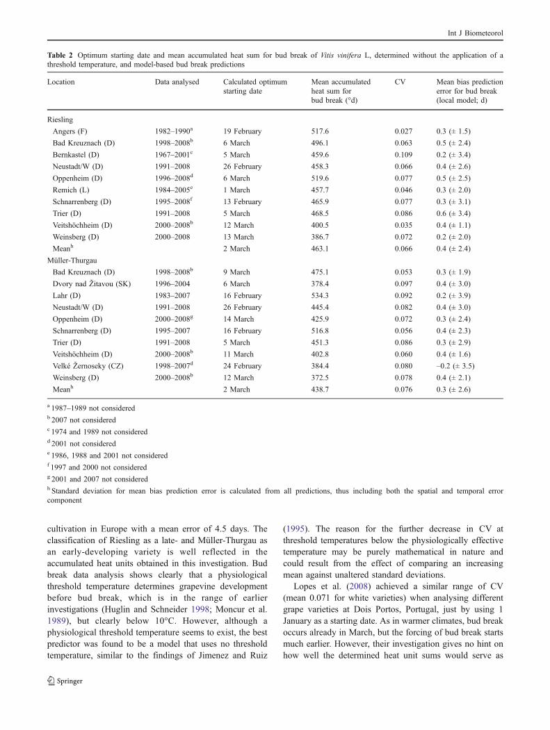
Although the pattern in Fig. 1 confirms that modelsusing degree-days with threshold temperatures lower than5°C will not predict bud break with much higher accuracy,it is evident that CV can be improved slightly by usinglower threshold temperatures. For this reason, optimumstarting date and heat sum were once again determined for amodel using no threshold temperature (Table 2). Here, themean optimum starting date was 2 March for both varieties,including an error of ± 9 days for Riesling and ± 10 daysfor Müller-Thurgau, respectively, and the mean heat sumaccumulated until bud break was 463.1±43.6°d for Rieslingand 438.7±57.0°d for Müller-Thurgau, respectively.

Predicting bud break with local and generalised parameters

In a cross validation, a general model using the thresholdtemperature and the mean parameters obtained from thisinvestigation would predict bud break of Riesling grapevine

Fig. 3 Locations of phenologi-cal observations for grapevineand main areas of viticulture inEurope (grey)

Int J Biometeorol

at all sites on average 0.6 days later than observed, with astandard error of ± 4.6 days (Table 3). Using site-specificparameters, the model would improve to a prediction of budbreak 0.6 days later than observed, with ± 2.6 days accuracy(Table 1). For Müller-Thurgau grapevines, a general modelwould predict average bud break 0.1 days too early,accepting an error of ± 4.6 days (Table 3). The local modelwould yield an accuracy of ± 3.2 days when predictingaverage bud break 0.5 days later than observed (Table 1).

Using the general model without the threshold temper-ature revealed only a marginal improvement for Rieslingbud break prediction at all sites, reducing the error by

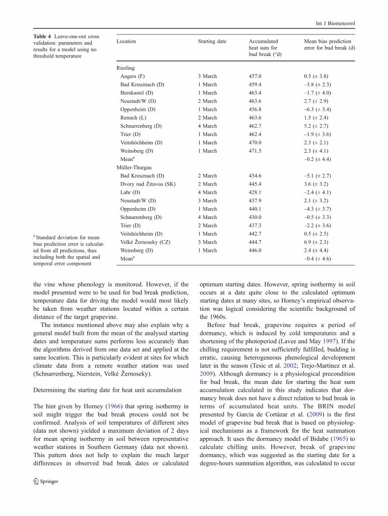
0.1 days. For Müller-Thurgau, no further improvement wasachieved (Table 4). Applying local parameters, an improve-ment of prediction accuracy by 0.2 days for Riesling and0.6 days for Müller-Thurgau was achieved (Table 2).

Discussion

Predicting bud break

The presented approach enables determining bud break ofV. vinifera at different sites at the northern boundary of vine

Table 1 Threshold temperature, optimum starting date, mean accumulated heat sum and model-based predictions for bud break of Vitis viniferaL. °d Degree days, CV Coefficient of variation, F France, D Germany, L Luxemburg, SK Slovakia, CZ Czech Republic

Location Data analysed Calculatedthresholdtemperature (°C)

Calculatedoptimumstarting date

Mean accumulatedheat sum forbud break (°d)

CV Mean dateobserved forbud break

Mean biasprediction errorfor bud break(local model; d)

Riesling

Angers (F) 1982–1990a 6.0 3 March 173.2 0.021 23 April 0.5 (± 0.8)

Bad Kreuznach (D) 1998–2008b 5.4 22 February 242.3 0.085 1 May 0.8 (± 2.7)

Bernkastel (D) 1967–2001c 6.2 27 February 170.3 0.125 29 April 0.4 (± 4.0)

Neustadt/W (D) 1991–2008 5.8 25 February 185.0 0.086 21 April 0.8 (± 2.9)

Oppenheim (D) 1996–2008d 6.1 6 March 218.1 0.117 30 April 1.0 (± 3.3)

Remich (L) 1984–2005e 5.9 28 February 177.1 0.123 27 April 0.9 (± 4.0)

Schnarrenberg (D) 1995–2008f 5.9 14 February 166.3 0.110 25 April 0.3 (± 2.8)

Trier (D) 1991–2008 6.5 5 March 169.4 0.111 26 April 0.6 (± 3.0)

Veitshöchheim (D) 2000–2008b 5.2 12 March 185.4 0.085 28 April 0.5 (± 2.0)

Weinsberg (D) 2000–2008 5.7 12 March 174.1 0.141 24 April 0.4 (± 2.8)

Meanh 5.9 1 March 186.1 0.100 0.6 (± 2.6)

Müller-Thurgau

Bad Kreuznach (D) 1998–2008b 5.2 9 March 226.3 0.086 29 April 0.4 (± 2.4)

Dvory nad Žitavou (SK) 1996–2004 6.9 6 March 130.8 0.117 21 April 0.6 (± 2.5)

Lahr (D) 1983–2007 6.9 16 February 174.6 0.132 24 April 0.6 (± 4.7)

Neustadt/W (D) 1991–2008 6.1 25 February 165.2 0.112 20 April 1.0 (± 3.2)

Oppenheim (D) 1997–2008g 5.5 2 March 219.7 0.132 24 April 0.9 (± 3.0)

Schnarrenberg (D) 1995–2007 5.6 16 February 215.2 0.117 23 April 0.6 (± 3.0)

Trier (D) 1991–2008 6.6 5 March 156.7 0.102 25 April 0.2 (± 2.7)

Veitshöchheim (D) 2000–2008b 5.2 11 March 186.1 0.120 27 April 0.6 (± 3.2)

Velké Žernoseky (CZ) 1998–2007d 5.1 24 February 165.7 0.143 26 April –0.1 (± 4.7)

Weinsberg (D) 2000–2008b 5.6 12 March 162.3 0.162 22 April 0.5 (± 3.3)

Meanh 5.9 1 March 180.3 0.122 0.5 (± 3.2)

a 1987–1989 not consideredb 2007 not consideredc 1974 and 1989 not consideredd 2001 not considerede 1986, 1988 and 2001 not consideredf 1997 and 2000 not consideredg 2001 and 2007 not consideredh Standard deviation for mean bias prediction error is calculated from all predictions, thus including both the spatial and temporal error component

Int J Biometeorol

cultivation in Europe with a mean error of 4.5 days. Theclassification of Riesling as a late- and Müller-Thurgau asan early-developing variety is well reflected in theaccumulated heat units obtained in this investigation. Budbreak data analysis shows clearly that a physiologicalthreshold temperature determines grapevine developmentbefore bud break, which is in the range of earlierinvestigations (Huglin and Schneider 1998; Moncur et al.1989), but clearly below 10°C. However, although aphysiological threshold temperature seems to exist, the bestpredictor was found to be a model that uses no thresholdtemperature, similar to the findings of Jimenez and Ruiz

(1995). The reason for the further decrease in CV atthreshold temperatures below the physiologically effectivetemperature may be purely mathematical in nature andcould result from the effect of comparing an increasingmean against unaltered standard deviations.

Lopes et al. (2008) achieved a similar range of CV(mean 0.071 for white varieties) when analysing differentgrape varieties at Dois Portos, Portugal, just by using 1January as a starting date. As in warmer climates, bud breakoccurs already in March, but the forcing of bud break startsmuch earlier. However, their investigation gives no hint onhow well the determined heat unit sums would serve as

Table 2 Optimum starting date and mean accumulated heat sum for bud break of Vitis vinifera L, determined without the application of athreshold temperature, and model-based bud break predictions

Location Data analysed Calculated optimumstarting date

Mean accumulatedheat sum forbud break (°d)

CV Mean bias predictionerror for bud break(local model; d)

Riesling

Angers (F) 1982–1990a 19 February 517.6 0.027 0.3 (± 1.5)

Bad Kreuznach (D) 1998–2008b 6 March 496.1 0.063 0.5 (± 2.4)

Bernkastel (D) 1967–2001c 5 March 459.6 0.109 0.2 (± 3.4)

Neustadt/W (D) 1991–2008 26 February 458.3 0.066 0.4 (± 2.6)

Oppenheim (D) 1996–2008d 6 March 519.6 0.077 0.5 (± 2.5)

Remich (L) 1984–2005e 1 March 457.7 0.046 0.3 (± 2.0)

Schnarrenberg (D) 1995–2008f 13 February 465.9 0.077 0.3 (± 3.1)

Trier (D) 1991–2008 5 March 468.5 0.086 0.6 (± 3.4)

Veitshöchheim (D) 2000–2008b 12 March 400.5 0.035 0.4 (± 1.1)

Weinsberg (D) 2000–2008 13 March 386.7 0.072 0.2 (± 2.0)

Meanh 2 March 463.1 0.066 0.4 (± 2.4)

Müller-Thurgau

Bad Kreuznach (D) 1998–2008b 9 March 475.1 0.053 0.3 (± 1.9)

Dvory nad Žitavou (SK) 1996–2004 6 March 378.4 0.097 0.4 (± 3.0)

Lahr (D) 1983–2007 16 February 534.3 0.092 0.2 (± 3.9)

Neustadt/W (D) 1991–2008 26 February 445.4 0.082 0.4 (± 3.0)

Oppenheim (D) 2000–2008g 14 March 425.9 0.072 0.3 (± 2.4)

Schnarrenberg (D) 1995–2007 16 February 516.8 0.056 0.4 (± 2.3)

Trier (D) 1991–2008 5 March 451.3 0.086 0.3 (± 2.9)

Veitshöchheim (D) 2000–2008b 11 March 402.8 0.060 0.4 (± 1.6)

Velké Žernoseky (CZ) 1998–2007d 24 February 384.4 0.080 –0.2 (± 3.5)

Weinsberg (D) 2000–2008b 12 March 372.5 0.078 0.4 (± 2.1)

Meanh 2 March 438.7 0.076 0.3 (± 2.6)

a 1987–1989 not consideredb 2007 not consideredc 1974 and 1989 not consideredd 2001 not considerede 1986, 1988 and 2001 not consideredf 1997 and 2000 not consideredg 2001 and 2007 not consideredh Standard deviation for mean bias prediction error is calculated from all predictions, thus including both the spatial and temporal errorcomponent

Int J Biometeorol

predictors at other locations. Since no data from warmerclimates were analysed for the present study, the result atthis stage is considered valid only for climates with coolwinters, providing temperatures cold enough for grapevinedormancy.

Physiological implications of the results

Although a satisfying degree of accuracy was achieved, themodel still does not help to clarify if any factor other thantemperature influences bud break. The analysis indicatesthat there is a period of time in late winter during whicheven longer periods of temperatures above assumed thresh-olds would have no impact on bud break. From theopposite perspective, applying the heat sum approach witha starting date of 15 March as proposed by Alleweldt andHofäcker (1975) would ignore degree-days significantlyimportant for bud break calculation at some sites. Astatistical analysis of long-term average climatic parameterssuch as radiation, precipitation, minimum and maximumtemperatures, and the local water balance (data not shown)revealed no significant influence of any of these parameterson bud break. Consideration of humidity data, as suggested

by Due et al. (1993), also did not yield any improvementsin prediction (data not shown).

However, the facts that (1) the heat sum approach yieldsa difference of more than 5 days in predicting bud break atsites within 60 km distance, and (2) a standard error of 9 ̄–10 days for the optimum starting date was found, indicatesthat more information than just temperature is required toexplain bud break.

One possible explanation could be that the weather datagenerally was not recorded directly adjacent to the vinewhose phenology was observed. The weather stations areoften located up to a few hundred metres away and maystand a little higher or lower in altitude. Indeed, for somesites weather data had to be obtained from weather stationsa few kilometres away. This explanation is supported by thefact that the analysis carried out to determine the optimumstarting date was very sensitive to weather stations beingrelocated during the record. In such cases, the iterationwould not yield a significant minimum and therefore thedata sets were truncated for analysis. Consequently, the dataobtained in this investigation would not allow anyhypothesis on grapevine physiology to be tested. For thispurpose, the temperature needs to be recorded directly at

Location Thresholdtemperature (°C)

Starting date Accumulatedheat sum forbud break (°d)

Mean biasprediction errorfor bud break (d)

Riesling

Angers (F) 5.9 1 March 187.6 1.7 (± 1.2)

Bad Kreuznach (D) 5.8 2 March 179.9 –3.7 (± 3.3)

Bernkastel (D) 5.9 1 March 187.9 0.8 (± 3.8)

Neustadt/W (D) 5.9 1 March 186.2 2.6 (± 3.5)

Oppenheim (D) 5.9 28 February 182.6 –6.6 (± 2.8)

Remich (L) 5.9 1 March 187.1 3.0 (± 4.6)

Schnarrenberg (D) 5.9 3 March 188.3 4.9 (± 3.0)

Trier (D) 5.8 1 March 188.0 –1.3 (± 3.3)

Veitshöchheim (D) 5.9 28 February 186.2 2.3 (± 2.6)

Weinsberg (D) 5.9 28 February 187.5 1.1 (± 3.9)

Meana 0.6 (± 4.6)

Müller-Thurgau

Bad Kreuznach (D) 5.9 28 February 175.1 –4.5 (± 3.0)

Dvory nad Žitavou (SK) 5.8 28 February 185.8 2.3 (± 3.3)

Lahr (D) 5.8 2 March 180.9 –2.7 (± 4.0)

Neustadt/W (D) 5.8 1 March 181.9 2.4 (± 3.6)

Oppenheim (D) 5.9 1 March 175.9 –3.3 (± 3.5)

Schnarrenberg (D) 5.9 1 March 176.4 –1.5 (± 4.4)

Trier (D) 5.8 2 March 182.9 –0.8 (± 2.7)

Veitshöchheim (D) 5.9 28 February 179.6 1.6 (± 3.5)

Velké Žernoseky (CZ) 6.0 2 March 181.9 7.1 (± 3.0)

Weinsberg (D) 5.9 28 February 182.3 2.6 (± 3.7)

Meana –0.1 (± 4.6)

Table 3 Leave-one-out crossvalidation: parameters andresults for a model using athreshold temperature

a Standard deviation for meanbias prediction error is calculat-ed from all predictions, thusincluding both the spatial andtemporal error component

Int J Biometeorol

the vine whose phenology is monitored. However, if themodel presented were to be used for bud break prediction,temperature data for driving the model would most likelybe taken from weather stations located within a certaindistance of the target grapevine.

The instance mentioned above may also explain why ageneral model built from the mean of the analysed startingdates and temperature sums performs less accurately thanthe algorithms derived from one data set and applied at thesame location. This is particularly evident at sites for whichclimate data from a remote weather station was used(Schnarrenberg, Nierstein, Velké Žernoseky).

Determining the starting date for heat unit accumulation

The hint given by Horney (1966) that spring isothermy insoil might trigger the bud break process could not beconfirmed. Analysis of soil temperatures of different sites(data not shown) yielded a maximum deviation of 2 daysfor mean spring isothermy in soil between representativeweather stations in Southern Germany (data not shown).This pattern does not help to explain the much largerdifferences in observed bud break dates or calculated

optimum starting dates. However, spring isothermy in soiloccurs at a date quite close to the calculated optimumstarting dates at many sites, so Horney’s empirical observa-tion was logical considering the scientific background ofthe 1960s.

Before bud break, grapevine requires a period ofdormancy, which is induced by cold temperatures and ashortening of the photoperiod (Lavee and May 1997). If thechilling requirement is not sufficiently fulfilled, budding iserratic, causing heterogeneous phenological developmentlater in the season (Tesic et al. 2002; Trejo-Martínez et al.2009). Although dormancy is a physiological preconditionfor bud break, the mean date for starting the heat sumaccumulation calculated in this study indicates that dor-mancy break does not have a direct relation to bud break interms of accumulated heat units. The BRIN modelpresented by García de Cortázar et al. (2009) is the firstmodel of grapevine bud break that is based on physiolog-ical mechanisms as a framework for the heat summationapproach. It uses the dormancy model of Bidabe (1965) tocalculate chilling units. However, break of grapevinedormancy, which was suggested as the starting date for adegree-hours summation algorithm, was calculated to occur

Location Starting date Accumulatedheat sum forbud break (°d)

Mean bias predictionerror for bud break (d)

Riesling

Angers (F) 3 March 457.0 0.5 (± 3.8)

Bad Kreuznach (D) 1 March 459.4 –3.8 (± 2.3)

Bernkastel (D) 1 March 463.4 –1.7 (± 4.0)

Neustadt/W (D) 2 March 463.6 2.7 (± 2.9)

Oppenheim (D) 1 March 456.8 –6.3 (± 3.4)

Remich (L) 2 March 463.6 1.5 (± 2.4)

Schnarrenberg (D) 4 March 462.7 5.2 (± 2.7)

Trier (D) 1 March 462.4 –1.9 (± 3.6)

Veitshöchheim (D) 1 March 470.0 2.3 (± 2.1)

Weinsberg (D) 1 March 471.5 2.3 (± 4.1)

Meana –0.2 (± 4.4)

Müller-Thurgau

Bad Kreuznach (D) 2 March 434.6 –5.1 (± 2.7)

Dvory nad Žitavou (SK) 2 March 445.4 3.6 (± 3.2)

Lahr (D) 4 March 428.1 –2.4 (± 4.1)

Neustadt/W (D) 3 March 437.9 2.1 (± 3.2)

Oppenheim (D) 1 March 440.1 –4.3 (± 3.7)

Schnarrenberg (D) 4 March 430.0 –0.5 (± 3.3)

Trier (D) 2 March 437.3 –2.2 (± 3.6)

Veitshöchheim (D) 1 March 442.7 0.5 (± 2.5)

Velké Žernoseky (CZ) 3 March 444.7 6.9 (± 2.3)

Weinsberg (D) 1 March 446.0 2.4 (± 4.4)

Meana –0.4 (± 4.6)

Table 4 Leave-one-out crossvalidation: parameters andresults for a model using nothreshold temperature

a Standard deviation for meanbias prediction error is calculat-ed from all predictions, thusincluding both the spatial andtemporal error component

Int J Biometeorol

as early as in December and for this reason did not improvethe predictive quality of the regular degree-day model usedin this investigation. The chilling unit accumulationalgorithms of Cannell and Smith (1983) or Cesaraccio etal. (2004) also did not lead to any better results.

A photoperiodic trigger for bud break initiation, similarto the day-length requirement of annual plants, is imagin-able (Imaizumi and Kay 2006; Tisserand 1875). Such anapproach is applied in some phenological models for annualspecies (Robertson 1968) and for trees (Kramer 1994).Experiments with grapevine shoots revealed that dormancyis induced by low temperatures or a shortening photoperiodor a combination of both factors, depending on the variety(Fennell and Hoover 1991; Schnabel and Wample 1987).Furthermore, bud break quantity is influenced by chillingintensity (Dokoozlian 1999). Beyond this, large numbers ofday-length experiments with grapevine were conducted inthe 1960s (Alleweldt 1967); however, they all concentratedon the impact of day-length on vegetative growth orinduction of dormancy. To the best of the author'sknowledge, no experiment in which the photoperiod wastested for its impact on grapevine post-dormancy has beenconducted.

What happens in the years excluded?

A clear minimum of CV during the iteration was sometimesmasked by data from one or more years in the respectivedata set. As mentioned above, relocation of a weatherstation during the record period causes such an effect. Butmistakes made during the observation of grapevine phe-nology could also impair the suitability of that year’s data.In some years, where bud break lasts over several days, theexact day when green tips are clearly visible at, on average,

every second vine is hard to determine. The year 2007 wasan exceptional year, with an unusually warm winter(Fig. 4). At several locations, the 2007 data masked theglobal CV minimum in the iterative procedure for determi-nation of the optimum starting date and thus had to beexcluded (Table 5). This raises the question of how thepost-dormancy period of the grapevine was affected in thisparticular winter.

As shown for the Müller-Thurgau variety (Table 3), in2007 grapevines accumulated significantly fewer heat unitsfrom the locally determined starting point to bud break,using the local model without threshold temperature. Thisseems to contradict the assumptions made for those modelsthat include dormancy break, in which the amount of heatunits to be accumulated for bud break is reduced when thepreceding winter has been very cold (Cannell and Smith1983), or in which the accumulation of heat units does notstart until the chilling requirement is fulfilled (Hänninen1990). In the present case, the accumulation of heat unitswas apparently triggered earlier in 2007 than in other years.The triggering event itself cannot be isolated here.However, the observed effect contradicts the notion ofphotoperiod as a single trigger.

Applicability of the model in climate change scenarios

One may ask if years that are warmer than usual wouldgenerally outflank a statistical model like this and if, in thiscase, such a model becomes useless in a warming climate?The answer is yes and no. Yes, because if, in warm winters,

Fig. 4 Accumulated heat sums from 1 August of the previous year atVeitshöchheim for the years 2000 to 2008. Year 2007 is highlightedfor its temperature anomaly

Table 5 Bud break of V. vinifera cv. Müller-Thurgau recordedbetween 2000 and 2008, and heat sums accumulated until bud breakat those sites where the 2007 data had to be excluded in order toidentify the starting date for heat unit accumulation

Year Budbreak

Heat suma

Veitshoechheim BadKreuznach

Weinsberg Oppenheim

Julianday

d

2000 116 394.3 451.2 337.1 366.5

2001 122 423.8 484.6 366.7 458.4

2002 118 406.1 466.0 322.4 455.0

2003 117 394.7 435.3 421.7 450.6

2004 117 390.3 504.0 368.4 422.7

2005 115 408.3 466.9 360.4 418.2

2006 122 408.2 459.3 376.4 430.6

2007 106 321.6b 368.7b 246.8b 282.9b

2008 122 378.1 425.6 369.1 477.5

a Threshold temperature = 0°C, local starting dateb Significant outlier; Grubbs’ test, α = 0.05

Int J Biometeorol

a physiological mechanism applies that is not sufficientlyreflected by using the heat summation approach with afixed starting date, any mechanistic model would bepreferable to the statistic approach; and no, because theheat units to be accumulated for grapevine until bud breakshowed no significant trend in the years investigated.However, until now there has been no mechanistic modelavailable for physiological processes occurring in a dor-mant bud, and the crucial processes during the differentphases of bud dormancy are even now not yet fully under-stood (Lavee and May 1997). Semi-mechanistic modelsusing a chilling requirement to explain the observed budbreak data do reach the predictive quality of the heatsummation model with optimised but fixed starting date, aswas shown by Kwon et al. (2008). However, the algorithmused by these authors for their investigation in Korea(Cesaraccio et al. 2005) requires experimentally derivedparameters, which are not yet available for Europe.

Conclusions

The predictive quality of a statistical model for grapevinebud break depends largely on the representativeness of theavailable climate data for the grapevine production area.Effectively, the sensitivity of the heat accumulation ap-proach hampers its application as a general model forgrapevine bud break prediction on a continental scale.Nevertheless, when applied to Northern European produc-tion areas, an average error of 4.5 days for prediction isfound. However, determination of bud break is a precon-dition for the simulation of subsequent stages of grapevinephenology. As such, the presented phenology model ismore accurate in predicting bud break than any otherapproach currently available and can, with caution, be usedfor simulating future growth scenarios of Northern Euro-pean grapevine. Improved understanding of the physiolog-ical processes triggered during the post-dormancy period,and their sensitivity to environmental factors, will mostlikely lead to better algorithms that allow regional methodsto be applied to climate data and the consideration ofmicrometeorology effects, thus leading to a more accurateprediction of bud break.

Acknowledgements The author gratefully acknowledges the contri-bution of the German Viticulture Research facilities in Bad Kreuznach(E. Müller), Bernkastel-Kues (M. Maixner), Freiburg (H.J. Stuecklin),Oppenheim (J. Wagenitz), Neustadt a.d.W. (B. Ziegler), Trier (E.Kohl), Veitshöchheim (H. Hofmann) and Weinsberg (D. Rupp), of theInstitute for Physics and Meteorology at Hohenheim University,Germany (I. Henning-Müller), of the Viticulture Research Instituteof Remich, Luxemburg (S. Fischer), of the Slovak HydrometeorologicalInstitute at Bratislava (P. Nejedlik), of the Czech HydrometerologicalInstitute at Ústí nad Labem (L. Hájková) and of INRA-Agroclim, France

(I. Garcia de Cortazar). Furthermore, many thanks are expressed to F.-M.Chmielewski (Humboldt-University of Berlin) and to I. Garcia deCortazar for valuable comments on the chosen approach.

References

Abrami G (1972) Optimum mean temperature for plant growthcalculated by a new method of summation. Ecology 53:893–900

Allen JC (1976) Modified sine wave method for calculating degreedays. Environ Entomol 5:388–396

Alleweldt G (1960) Untersuchungen über denAustrieb derWinterknospenvon Reben. Vitis 2:134–152

Alleweldt G (1967) Grapevine physiology. Research results 1961–1964. Vitis 6:63–81

Alleweldt G, Hofäcker W (1975) Einfluß von Umweltfaktoren aufAustrieb, Blüte, Fruchtbarkeit und Triebwachstum bei der Rebe.Vitis 14:103–115

Arnold CY (1960) Maximum-minimum temperatures as a basis forcomputing heat units. Proc Am Soc Hortic Sci 74:430–445

Baskerville GL, Emin P (1969) Rapid estimation of heat accumulationfrom maximum and minimum temperatures. Ecology 50:514–517

Besselat B, Drouet G, Palagos B (1995) Méthodologie pourdéterminer le besoin thermique nécessaire au départ de lafloraison de la vigne. J Int Sci Vigne Vin 29:171–182

Bidabe B (1965) Contrôle de l'époque de floraison du pommier parune nouvelle conception de l'action de températures. C R AcadAgric Fr 49:934–945

Bindi M, Miglietta F, Gozzini B, Orlandini S, Seghi L (1997) Asimple model for simulation of growth and development ingrapevine (Vitis vinifera L.). I. Model description. Vitis 36:67–71

Burckhardt F (1860) Über die Bestimmung des Vegetationsnullpunktes.Verh Naturforsch Ges Basel 2:47–62

Buttrose MS, Hale CR (1973) Effect of temperature on developmentof the grapevine inflorescence after bud burst. Am J Enol Vitic24:14–16

Calo A, Zomasi D, Costacurta A, Biscaro S, Aldighiere R (1994) Theeffect of temperature thresholds on grapevine (Vitis spec.) bloom.An interpretative model. Riv Vitic Enol 47:3–14

Cannell MGR, Smith RI (1983) Thermal time, chill days andprediction of budburst in Picea sitchensis. J Appl Ecol 20:951–963

Cesaraccio C, Spano D, Snyder RL, Duce P (2004) Chilling andforcing model to predict bud-burst of crop and forest species.Agric For Meteorol 126:1–13

Cesaraccio C, Spano D, Snyder RL, Duce P (2005) Chilling andforcing model to predict bud-burst of crop and forest species(corrigendum to vol 126, 1–13, 2004). Agric For Meteorol129:211–211

Christiansen P (1969) Seasonal changes and distribution of nutritionalelements in Thompson Seedless grapevines. Am J Enol Vitic20:176–190

Chuine I, Kramer K, Hänninen H (2003) Plant development models.In: Schwartz MD (ed) Phenology: an integrative environmentalscience. Kluwer, Dordrecht, pp 217–235

de Réaumur RAF (1735) Observations du thermomètre, faites à Parispendant l'annee 1735, comparées avec celles qui ont été faitessous la ligne, á l'isle de France. á Alger et quelques unes des nosisles de l'Amérique. Memoires de l'Académie des Sciences deParis

Dokoozlian NK (1999) Chilling temperature and duration interact onthe budbreak of 'Perlette' grapevine cuttings. Hortscience34:1054–1056

Int J Biometeorol

Due G, Morris M, Pattison S, Coombe BG (1993) Modelinggrapevine phenology against weather—considerations based ona large data set. Agric For Metorol 65:91–106

Eckenrode CJ, Chapman RK (1972) Seasonal adult Cabbage MaggotDiptera-Anthomyiidae populations in field in relation to thermalunit accumulations. Ann Entomol Soc Am 65:151–156

Fennell A, Hoover E (1991) Photoperiod influences growth, buddormancy, and cold acclimation in Vitis labruscana and V.riparia. J Am Soc Hortic Sci 116:270–273

García de Cortázar I, Brisson N, Gaudillere JP (2009) Performance ofseveral models for predicting bud burst date of grapevine (Vitisvinifera L.). Int J Biometeorol 53:317–326

Gilbert N, Gutierrez AP (1973) Plant-aphid-parasite relationship. JAnim Ecol 42:323–337

Gutierrez AP, Williams DW, Kido H (1985) A model of grape growthand development: the mathematical structure and biologicalconsiderations. Crop Sci 25:721–728

Hänninen H (1990) Modelling bud dormancy release in trees fromcool and temperate regions. Acta For Fenn 213:1–47

Hickin RP, Vittum MT (1976) Importance of soil and air temperaturein spring phenoclimatic modeling. Int J Biometeorol 20:200–206

Horney G (1966) Die Vorhersage des Blühtermins der Reben.Weinberg Keller 13:263–273

Huglin P, Schneider C (1998) Biologie et écologie de la vigne. 2.Auflage. Lavoisier, Paris

Imaizumi T, Kay SA (2006) Photoperiodic control of flowering: notonly by coincidence. Trends Plant Sci 11:550–558

Jimenez J, Ruiz V (1995) Phenological development of Vitis viniferaL. in Castilla - La Mancha (Spain)—a study of 21 cultivars (10red and 11 white cultivars). Acta Hortic 388:105–110

Kramer K (1994) Selecting a model to predict the onset of growth ofFagus Sylvatica. J Appl Ecol 31:172–181

Kwon EY, Jung JE, Chung U, Yun JI, Park HS (2008) Using thermaltime to simulate dormancy depth and bud-burst of vineyards inKorea for the twentieth century. J Appl Meteorol Climatol47:1792–1801

Lachenbruch PA, Mickey MR (1968) Estimation of error rates indiscriminant analysis. Technometrics 10:1–11

Lavee S, May P (1997) Dormancy of grapevine buds—facts andspeculation. Aust J Grape Wine Res 3:31–46

Lindsey AA (1963) Accuracy of duration temperature summing andits use for Prunus Serrulata. Ecology 44:149–151

Lindsey AA, Newman JE (1956) Use of official weather data in springtime—temperature analysis of an Indiana phenological record.Ecology 37:812–823

Lopes J, Eiras-Dias JE, Abreu F, Climaco P, Cunha JP, Silvestre J(2008) Thermal requirements, duration and precocity of pheno-logical stages of grapevine cultivars of the Portuguese collection.Cienc Tec Vitiv 23:61–71

Lorenz DH, Eichhorn KW, Bleiholder H, Klose R, Meier U, Weber E(1994) Phänologische Entwicklungsstadien der Weinrebe (Vitisvinifera L. ssp. vinifera). Vitic Enol Sci 49:66–70

Magoon CA, Culpepper CW (1932): Response of sweet corn tovarying temperatures from time of planting to canning maturity.US Dep Agric Tech Bull 312

May P (1964) Über die Knospen- und Infloreszenzentwicklung derRebe. Wein-Wiss 19:457–485

McIntyre GN, Kliewer WM, Lider LA (1987) Some limitations of thedegree-day system as used in viticulture in California. Am J EnolVitic 38:128–132

Moncur MW, Rattigan K, Mackenzie DH, McIntyre GN (1989) Basetemperatures for budbreak and leaf appearance of grapevines.Am J Enol Vitic 40:21–26

Nendel C, Kersebaum KC (2004) A simple model approach to simulatenitrogen dynamics in vineyard soils. Ecol Model 177:1–15

Peyer E, Koblet W (1966) Der Einfluss der Temperatur und derSonnenstunden auf den Blütezeitpunkt der Reben. Schweiz. Z.Obst-Weinbau 10:250–255

Pouget R (1988) Le débourrement des bourgeons de la vigne:méthode de prévision et principes d´établissement d´une échellede précocité de débourrement. Connais Vigne Vin 22:105–123

Robertson GW (1968) A bio-meteorological time scale for a cerealcrop involving day and night temperatures and photoperiod. Int JBiometeorol 12:191–223

Schnabel BJ, Wample RL (1987) Dormancy and cold hardiness inVitis vinifera L. cv. White Riesling as influenced by photoperiodand temperature. Am J Enol Vitic 38:265–272

Sevacherian V, Stern VM, Mueller AJ (1977) Heat accumulation fortiming Lygus (Hemiptera-(Heteroptera)-Miridae) control mea-sures in a safflower-cotton complex. J Econ Entomol 70:399–402

Tesic D, Woolley DJ, Hewett EW, Martin DJ (2002) Environmentaleffects on cv Cabernet Sauvignon (Vitis vinifera L.) grown inHawke's Bay, New Zealand. 1. Phenology and characterisation ofviticultural environments. Aust J Grape Wine Res 8:15–26

Tisserand E (1875) Mémoire sur la végétation dans les hauteslatitudes. Mémoires de la Société Central d'Agriculture Bouchard-Huzard, Paris, p 271

Trejo-Martínez MA, Orozco JA, Maguer-Vargas G, Carvajal-Millan E,Gardea AA (2009) Metabolic activity of low chilling grapevinebuds forced to break. Thermochim Acta 481:28–31

Wermelinger B, Baumgärtner J, Gutierrez AP (1991) A demographicmodel of assimilation and allocation of carbon and nitrogen ingrapevines. Ecol Model 53:1–26

Wielgolaski FE (1999) Starting dates and basic temperatures inphenological observations of plants. Int J Biometeorol 42:158–168

Williams DW, Andris HL, Beede RH, Luvisi DA, Norton MVK,Williams LE (1985) Validation of a model for the growth anddevelopment of the Thompson Seedless grapevine. II. Phenology.Am J Enol Vitic 36:283–289

Winkler AJ (1962) General viticulture. University of California Press,Berkeley

Wolfart A, Bogenrieder A, Becker N (1988) Climate and vinephenology—evaluation of a long-term series of observations atthree locations near Freiburg in Breisgau. Mitt Klosterneuburg38:108–119

Zalom FG, Goodell PB, Wilson LT, Barnett WW, Bentley WJ (1983)Degree-days: the calculation and use of heat units in pestmanagement. Division Agriculture and Natural Resources,University of California, Berkeley

Int J Biometeorol