Mapping nitrate in the global ocean using remotely sensed sea surface

temperature

Anna C. Switzer, Daniel Kamykowski, and Sara-Joan ZentaraDepartment of Marine, Earth and Atmospheric Sciences, North Carolina State University, Raleigh, North Carolina, USA

Received 17 May 2000; revised 18 July 2002; accepted 15 April 2003; published 27 August 2003.

[1] Nitrogen is the most broadly limiting factor for marine phytoplankton on ecologicaltimescales. Nitrate, as the most oxidized inorganic species, plays a significant role innitrogen availability based on nutrient flux to the euphotic zone from deeper waters, andis a major determinant of new production. Increased new production relates to highertrophic level abundance and to carbon dioxide drawdown from the atmosphere. Thepresent work is the first stage in the development of a technique to generate a scaled indexof nitrate availability in the surface waters of the global ocean using satellite-derivedtemperature data. The technique currently involves a fixed matrix of nitrate depletiontemperatures (NDT) and remotely-sensed sea surface temperature (SST) from themonthly-averaged AVHRR Pathfinder series. The magnitude of the difference betweenthese two temperatures at a given location indicates the degree of nitrate presence orabsence. Graded monthly nitrate presence/absence maps over a 10-year period werecreated based on the size of the difference between these two temperatures. A 10-yearaverage of these differences exhibits major nitrate distribution features similar to thoseobserved in maps based on National Oceanic Data Center archived measurements. Incontrast, monthly nitrate maps provide a unique and dynamic representation of nitrateavailability in the global ocean. This nutrient monitoring capability based on remotelysensed data can contribute to the estimation of new production in the global ocean,improving management of various world fisheries and improving estimation of theatmospheric draw down of carbon dioxide, a major greenhouse gas. INDEX TERMS: 4275

Oceanography: General: Remote sensing and electromagnetic processes (0689); 4845 Oceanography:

Biological and Chemical: Nutrients and nutrient cycling; KEYWORDS: nitrate availability, remote sensing,

nutrient depletion temperature, mapping

Citation: Switzer, A. C., D. Kamykowski, and S.-J. Zentara, Mapping nitrate in the global ocean using remotely sensed sea surface

temperature, J. Geophys. Res., 108(C8), 3280, doi:10.1029/2000JC000444, 2003.

1. Introduction

1.1. Background

[2] Nitrogen is one of the key elements in the biogeo-chemistry of the oceans [Harrison, 1992]. Nitrate, the mostoxidized form of nitrogen, is critical to our present under-standing of oceanic and atmospheric processes because itprovides the largest inorganic oceanic reservoir of thislimiting nutrient for most marine phytoplankton [Levituset al., 1993]. Phytoplankton growth supported by externalnitrogen sources like nitrate has been termed ‘‘new’’ pro-duction, whereas growth supported by recycled nitrogenprimarily in the form of ammonium, has been termed‘‘regenerated’’ production [Dugdale and Goering, 1967].Nitrate concentration can thus be indicative of the potentialfor nitrate-supported new production in surface waters[Levitus et al., 1993]. Although concepts related to upperocean food webs are undergoing revision [Legendre andRassoulzadegan, 1995; Azam, 1998], new production

remains in many ways the more anthropocentrically inter-esting fraction of total primary production. It is the portionthat supports higher trophic levels in the harvestable sizeclasses, and also indicates the amount of atmosphericcarbon dioxide that will be used for phytoplankton growth,thus eventually becoming available for burial on the sea-floor [Eppley and Peterson, 1979].[3] The temporal and spatial variation of nitrate concen-

tration in the oceans is large [Garside and Garside, 1995].Present sampling techniques used on board research vesselsor even at moored stations are inadequate when comparedto existing scales of fluctuation. In order to understand andeventually quantify the role of nitrate in the world’sbiogeochemistry, more representative methods for estimat-ing nitrate on ocean basin scales needs to be developed[Garside and Garside, 1995].[4] The connections between physical and biological

processes in the ocean have been a focus of recent marineresearch [Kamykowski, 1986]. As the understanding of theseconnections matures, technologies designed for a particularoceanographic discipline find applications in other relateddisciplines. Specifically, sea surface temperature (SST),

JOURNAL OF GEOPHYSICAL RESEARCH, VOL. 108, NO. C8, 3280, doi:10.1029/2000JC000444, 2003

Copyright 2003 by the American Geophysical Union.0148-0227/03/2000JC000444$09.00

36 - 1

which is a physical property of the ocean and primarilyruled by physical processes, can be detected by satellite-based sensors. Owing to the physical-biological link in theocean, SST can relate to biological and/or chemical pro-cesses [Kamykowski and Zentara, 1986]. For example, aportion of the solar radiation that heats the water and raisesits temperature is also used by phytoplankton to fuelphotosynthesis. Through photosynthesis, phytoplanktonutilize nutrients such as nitrate, phosphate, and silicate[Kamykowski, 1987; Minas and Codispoti, 1993]. Theobservation that nutrient concentration decreases as temper-ature increases suggests that these two processes are tightlycoupled in the upper ocean. Strickland [1967] first identifiedthis coupling using data collected off coastal California. Hefound that one could predict nitrate concentrations almost towithin experimental accuracy from a knowledge of temper-ature [Strickland, 1967]. Traganza et al. [1980] were the firstto apply this relationship to remotely sensed temperaturedata. They confirmed the inverse relationship of nutrientswith temperature via in situ measurements and then identi-fied the temperature and derived nutrient patterns associatedwith an area of upwelling off the coast of California viaremote sensing. Dugdale et al. [1989], Babin et al. [1991],Haldron and Probyn [1992], and Morin et al. [1993]reconfirmed the applicability of nutrient-temperature rela-tionships in remote sensing as applied to upwelling andtidally driven areas. Nutrient-temperature relationships canprovide information about the chemical structure of largeareas of the world ocean on temporal and spatial scales thatare otherwise unattainable [Kamykowski and Zentara, 1986].More recently, Carder et al. [1999] combined nutrient-temperature relationships and remote sensing to define bio-optical domains for chlorophyll-a algorithms.

1.2. Nitrate Depletion Temperatures

[5] Historical data collected at various locations in theworld ocean show the relationship between nitrate con-centration and temperature to be inverse [Zentara andKamykowski, 1977; Minas and Codispoti, 1993]. Whilethere is some scatter in any individual plot, there also aredefinite, regionally specific correlations between the twovariables. A generic version of these plots is shown inFigure 1. Specific plots at various latitudes are given byZentara and Kamykowski [1977].[6] Graphs of nitrate versus temperature have two fea-

tures that can be utilized in conjunction with remotelysensed SST to yield real-time information about the avail-ability of nitrate. The intercept at the temperature axis iscalled the nitrate depletion temperature (NDT), due to thefact that above this temperature, nitrate concentration is zeroas measured by traditional chemical methods [Parsons etal., 1984]. Below the NDT, the slope of the relationshipbecomes important as it can be used to calculate the specificconcentration of available nitrate at a certain SST. Althoughthis relationship holds throughout the upper ocean, thenitrate concentrations predicted with this satellite-basedtechnique only apply at the surface due to the fact thatpresent remote sensors can only sense sea surface temper-ature [Schluessel et al., 1990].[7] The slope and NDT vary with location. Latitude is

primary among the reasons for this variation [Kamykowski,1987] (but see Minas and Codispoti [1993] for additional

insight), due to the global gradient of solar radiation actingwith a phytoplankton growth capability that spans thenatural temperature range in the ocean [Eppley, 1972]. Inequatorial waters, there is relatively consistent heatingthroughout the year [Kirk, 1986], so the water temperaturethrough a relatively thick upper water column is high, withan upper limit primarily determined by evaporation rate[Pickard, 1963]. Nitrate that becomes available via upwell-ing events occurs in relatively high temperature water that isfurther heated as it nears the surface; therefore the NDTs inthis area occur at high temperatures. The opposite occurs inthe polar regions where sunlight is absent or very weakduring winter but almost continuous in summer [Kirk,1986]. The nitrate that is available here occurs in relativelycold water, but this water will also warm as it nears thesurface. Thus NDTs in these latitudes occur at lowertemperatures. The temperate latitudes experience tempera-ture ranges between these two extremes.[8] Longitudinal perturbations to the underlying latitudinal

dependence of the NDTs also occur. Typical ocean basincirculation can be considered to move water with aspecific nutrient-temperature relationship from one latitudeto another, as such the NDT can be used as a water masstracer similar to the use of temperature and salinity [Brown etal., 1989]. For example, in the northern Atlantic the GulfStream carries water from the tropics (high NDT) intolatitudes with lower inherent NDT. Conversely, the Califor-nia current in the northern Pacific brings water with a lowNDT into a higher NDT region. Therefore across a middlelatitude section of an ocean basin, the NDT typically is higheralong the western boundary than the eastern boundary.[9] NDT also is affected by vertical considerations. In

the normal vertical water column, nitrate concentrationsincrease with depth due to gravitational settling, while solarheating decreases with depth due to differential attenuationof the solar spectrum [Kirk, 1986]. Thus the nutrient-temperature relationship can vary as a result of the changingamount of energy available to heat a given water parcel perunit nitrate as depth increases. Consider two separate windevents, one yielding vertical mixing and the other yielding ahorizontal upwelling plume. Wind events that cause mixingin the upper layer cycle nutrients to the surface and backdown to depth. Thus, on average, a water parcel experiencesan attenuated version of the solar spectrum. In an upwellingwind event, where a nutrient-rich water parcel is horizon-tally drawn out at the surface and is thus exposed to abroader spectrum of solar radiation, the result is a greaterincrease in temperature rise per unit nitrate than in thevertical mixing event [Simpson and Dickey, 1981; Paulsonand Simpson, 1977]. Hence the temperature of this samenutrient-rich water rises more quickly on the surface asnutrients are utilized than in the vertically mixed case. Thisdifferential heating can lower the slope of the nutrient(y)-temperature(x) relationship and can shift the NDT to ahigher temperature in the upwelling plume case. Since theNDTs used here are based on all available data at a givenlocation, these two representative cases, namely the windmixed water column and local upwelling-like events, maybe blended in a single number representing the location.[10] Three instances in which the nutrient-temperature

relationship breaks down must also be considered. First,there are oxidation state preferences for nitrogen uptake by

36 - 2 SWITZER ET AL.: INTERANNUAL NITRATE AVAILABILITY MAPPING

phytoplankton [Harrison, 1992]. They prefer to use ammo-nium resulting from nitrogen cycling within the food web astheir nitrogen source when it is available [McCarthy, 1981].Ammonium is a recycled form of nitrogen that requires lessenergy to metabolize than nitrate. Therefore, in areas wherethere is a significant amount of ammonium available for useby phytoplankton, the nitrate-temperature relationship maychange in presently unpredictable ways [Harrison, 1992].The water will be heated with incoming solar energy, butnitrate may be utilized at a slower rate because of apreference for ammonium. Noting that the ultimate sourceof ammonium is often previously used nitrate, there may betime lags in the generation of significant amounts ofammonium during which nitrate will be the dominantnitrogen source.[11] A second consideration in the nitrate case is iron

availability, since the rate of nitrate utilization is iron depen-dent [Chisholm, 1995; de Baar, 1994]. The nitrate-temper-ature relationship may change slope with iron availability.The potential for iron limitation is documented in definedregions of the global ocean, specifically the Southern Ocean,equatorial Pacific, and subarctic Pacific [Hutchins andBruland, 1998; Takeda, 1998; Pondhaven et al., 1999].[12] Third, uncoupling occurs at the site of large fresh-

water plumes, such as the mouths of the Amazon andColumbia Rivers. Here freshwater provides an independentsource of nitrate that cannot be accounted for via a temper-ature indicator associated with the vertical water column.Therefore satellite remote sensing of salinity [Goodberlet etal., 1997] may be required before nitrate predictionbecomes feasible in areas influenced by river run-off.[13] Despite the limitations that may confound the inter-

pretation of the nitrate-temperature relationship, the globalsurvey [Kamykowski, 1986] demonstrates a broad utility.The present paper will first use the physical-biologicalconnection between temperature and nitrate, representedby the NDT, to create global maps of nitrate availability

based on satellite-derived SST. Second, the significance ofthe patterns will be examined by comparison with the nitratemaps provided by NODC archived measurements. Third,qualitative comparisons between the seasonal global nitratepatterns and seasonal global phytoplankton pigment patternswill be made.

2. Methods

2.1. Extending the Existing Matrix of Nitrate DepletionTemperatures (NDT)

[14] Previous work by Zentara and Kamykowski [1977]and Kamykowski and Zentara [1986] provided the precursorto the present matrix. This included the creation of scatter-plots of nitrate(y) versus temperature(x) for 10� latitude by10� longitude squares (hereinafter referred to as ten-square)in the global ocean based on availability of data from theNational Oceanic Data Center (NODC) archive. Acknowl-edging the curvilinear shape of the nitrate versus tempera-ture relationships in the upper kilometer of the world ocean,cubic regressions of these scatterplots were calculated.Percentiles (25th, 50th, and 75th) also were determinedfor each scatterplot for the temperatures at which nitrate wasless than 5 uM in each ten-square.[15] In order to quantify nitrate depletion temperatures

(NDT), a subset of real roots [Selby, 1965], where nitrateconcentration along the trend of the scatterplot first equaledzero, were calculated for the cubic regressions. However,this data set left major portions of the world ocean basinsunrepresented (Figure 2a). To fill in the gaps, an appropriatepercentile for each ten-square was selected based on acomparison with cubic regression roots where both co-occurred. Where the regression roots were missing, thepercentile closest to the intercept on the x axis of thescatterplot was chosen to represent the NDT. These semi-quantitative determinations provided the coarse scale NDTsseen in Figure 2b. Table 1 gives the statistical characteristicsof the ten-square percentile and cubic regression analysis forthe NDTs used here (see Kamykowski and Zentara [1986]for further discussion). The coarse NDT matrix interpolatedto 0.5� resolution became the working matrix of NDTsas applied to satellite data of sea surface temperature(Figure 2c). Note that since the cubic analysis did notproduce slope values to complement the NDT values, onlyrelative presence/absence rather than actual nitrate concen-trations are provided here. This difference will becomesignificant in later comparisons.

2.2. Obtaining Matrices of Sea Surface Temperature

[16] These data were obtained from the NASA PhysicalOceanography Distributed Active Archive Center at the JetPropulsion Laboratory, California Institute of Technology.Specifically, they were a mixture of ‘‘Best’’ and ‘‘All’’ (peryearly availability), ascending, and at 54 km resolution.

2.3. Matching Grid Nodes

[17] One additional step was necessary to match thenodes of the NDT and SST matrices. The SST values fromAVHRR are presented at the centers of the 0.5� squareswhile the NDT matrix presented values at the corners. To fixthis discrepancy, the NDT matrix was actually interpolatedto a resolution of 0.25�, which gave values at the centers aswell as the corners. From this array, every other point in

Figure 1. Generic nitrate-temperature relationship. Whensubtracting the NDT from the SST, a negative numberindicates nitrate presence, and zero or a positive numberindicates nitrate absence.

SWITZER ET AL.: INTERANNUAL NITRATE AVAILABILITY MAPPING 36 - 3

Figure 2. (a) Cubic regression roots in the range of the data from the nitrate-temperature scatterplots at10� latitude/longitude resolution for the world oceans. (b) Nitrate depletion temperatures at 10� latitude/longitude resolution contoured at approximately 2.5� Celsius intervals to show the general trend of thedata. (c) Nutrient depletion temperatures at 0.5� latitude/longitude resolution contoured at 2.5� Celsiusintervals.

36 - 4 SWITZER ET AL.: INTERANNUAL NITRATE AVAILABILITY MAPPING

both the latitudinal and longitudinal directions wasextracted to finalize a matrix which matched the SST arraysin scale and location. This interpolation and extractionprocess was accomplished via triangulation with linearinterpolation using the Surfer software package.

2.4. Subtracting the Two Matrices and MappingResults

[18] Utilizing Interactive Data Language (IDL), a simplematrix subtraction was made. SST-NDT yielded a resultantmatrix in units of temperature (�C) which had three possibletypes of numbers (refer to Figure 1): (1) If SST was less

than the NDT (negative result), then nitrate was available;(2) if SST was greater than or equal to the NDT (positiveresult or zero), then nitrate was depleted; and (3) in the caseof land or a missing value due to cloud cover in the SSTdata set, a dummy value was assigned.[19] Contoured images were created to show the degree to

which nitrate was either present or absent. Essentially, as theSST-NDT difference increased, nitrate was either moreavailable (increased negative number) or more depleted(increased positive number). Specific values of both nega-tive and positive differences were then contoured to derive ascaled index of nitrate availability in all of the ocean basins.

2.5. ‘‘Groundtruthing’’ the Images With HistoricalData

[20] A decadal average was computed to support aqualitative comparison of the nitrate availability mapscreated with this technique. After all of the months fromJanuary 1987 through December 1996 were contoured asdescribed above, an average of these 120 maps was com-puted. All positive differences between SST and NDT werefirst set equal to zero. This pretreatment rescaled nitrateabsence values to zero in the SST-NDT matrix to match thenitrate scale, which had no negative values.[21] This average map of contoured SST-NDT (Figure 3a)

was then compared to a global historic picture provided bythe Ocean Atlas, which is a continuation of the Climato-logical Atlas of the World Ocean [Levitus et al., 1994]available through the NODC website. This presentation ofhistoric nutrient values was created by averaging datacollected on cruises from 1900 through March 1993. Thedata, representing a range of techniques and varying tem-poral coverage, provide a global view on a 1� scale. Sincethe nitrate map exhibited some irregularities (Figure 3d), anitrate proxy map (Figure 3c) was derived from the phos-phate map which had more complete coverage. As arepresentative approximation, phosphate was multiplied by

Table 1. Statistical Characteristics of the 10� Latitude by 10�Longitude Percentile and Cubic Regression Analyses Described by

Kamykowski [1986] for 17 Latitudinal Bandsa

Lat AvMed Range Error

85 �0.91 0.58 3.0875 0.66 1.86 2.7565 3.75 3.49 3.3255 6.67 2.50 6.1945 10.99 7.44 5.3035 17.43 3.77 4.1325 22.34 4.41 4.0315 25.94 2.69 4.425 27.10 1.83 3.49�5 26.02 2.05 3.53�15 24.07 3.86 3.54�25 19.25 3.93 3.14�35 16.05 3.22 2.73�45 10.62 2.67 3.69�55 6.09 0.80 3.65�65 �0.41 0.26 4.09�75 �0.89 0.24 4.10

aLat is the center of the latitudinal band, AvMed is the average median(50th percentile), Range is the average difference between the 25th and 75thpercentiles, and Error is the average error of the data points around the bestfit cubic regression curves. Positive latitudes are north; negative latitudesare south.

Figure 3. (a) Average nitrate availability for January 1987 through December 1996 based on 120monthly determinations. (b) Difference between Figures 3a and 3c after normalizing each and rescalingfrom 1–100. (c) Phosphate concentration map from World Ocean Atlas multiplied by 15 to becomenitrate proxy map. (d) Nitrate concentration maps from Levitus et al. [1993]. Green areas show where thedifference lies between ±33%. Nitrate proxy values exceeding the NDT-based values by more than 33%are shown in orange, and the converse in blue.

SWITZER ET AL.: INTERANNUAL NITRATE AVAILABILITY MAPPING 36 - 5

15 as defined by the Redfield ratio of phosphate:nitrate inseawater [Redfield, 1958].[22] To make a direct comparison, the Ocean Atlas nitrate

proxy map was scaled to 0.5� to parallel the NDT-derivedmap. Recall that the Ocean Atlas map has units of M nitrate-nitrogen, while the NDT map, as a difference of the SST andthe NDT, has units of �C. Bothmaps were normalized by theirmaximum values to a scale of 0 to 100%. Once normalized,the difference at each locationwas then calculated (Figure 3b).

2.6. Obtaining Ocean Color Data

[23] Ocean color data were provided by the SeaWiFSProject, NASA/Goddard Space Flight Center and ORB-IMAGE (http://seawifs.gsfc.nasa.gov/cgibrs/level3.pl). Notethat global maps obtained from this web site were notmanipulated before printing.

3. Results

3.1. Monthly Maps of Sea Surface Nitrate

[24] The NDT matrix was subtracted from each of themonthly averaged SST matrices for January 1987 throughDecember 1996 to produce 120 nitrate availability maps.Thirty-six of these (January 1987 through December 1989)are displayed in Figure 4. This particular time span waschosen to include both El Nino and La Nina conditions, asmeasured with NOAA’s Multivariate El Nino SouthernOscillation Index (MEI). The maps show whether the SSTis less than (green = SST < NDT) or greater than (blue =SST > NDT) the NDT by virtue of color, and also how far agiven SST is from the NDT at that location by virtue of thecolor shade within the green or blue codes. An arbitrary cut-off value of ±20�C on either side of the NDT was used toeliminate extreme values.[25] Though the main division in the nitrate availability

maps is between nitrate presence and absence, a moredetailed and interesting story is given by the contour levelswithin the presence and absence categories. On the positiveside of SST-NDT, or where nitrate is depleted, a morepositive value indicates a higher degree of water columnstratification. A lighter blue color (small positive SST-NDT)indicates this water has been heated less intensely than waterof darker blue color (large positive SST-NDT). In general, thedarker blue region lies over a water column that has a strongertemperature gradient between the sea surface and the deepnutrient pool, and would require a stronger wind event tobring nutrients from depth. On the negative side of SST-NDT,or where nitrate is available, a more negative value indicates arelatively higher nitrate concentration. The relative nature isdue to the unspecified but generally negative slope in mostnitrate-temperature plots as represented in Figure 1.[26] Note that there are areas within all of the maps that

need to be disregarded due to either a lack of NDT data and/or to the presence of a non-oceanic salinity value. The latterlist includes Hudson Bay, the Great Lakes region, the BalticSea, sections of the Mediterranean Sea, the Black Sea, theRed Sea, the Caspian Sea, and the Persian Gulf.

3.2. Validation of SST-NDT Approach

[27] In order to discern if the nitrate availability asdetermined by satellite SST is realistic, the SST-NDTpatterns are compared with actual nitrate values. A visual

comparison between a 10-year average of the NDT-basedmaps (Figure 3a) and the Levitus et al. [1994] nitrate(Figure 3d) and nitrate proxy maps (Figure 3c) showsgeneral agreement. The high-latitude regions, the largeequatorial upwelling region off northwestern South Amer-ica, and the most northwestern portions of the two majoroceans appear darkest green (high nitrate) in these maps.However, the Levitus-based nitrate map displays someunusual patterns. Specifically, there is a strip of ocean inthe central/western Pacific with anomalously high nitrate.Also, there are many unrepresented regions. These issuesare mostly eliminated in the nitrate proxy map (Figure 3c).In order to directly compare the nitrate proxy map and thesatellite-based map, each was normalized as previouslydescribed. By subtracting the two normalized versions andmapping the result, areas of major difference can be seen(Figure 3b). The majority of the global ocean falls within adifference range of ±33% (green color). Geographic areaswhere Levitus values exceed the NDT-based values by>33% can be seen in orange, and those where the NDT-based values exceed the Levitus values by >33% in blue.The total area covered by these latter large differences issmall, justifying the conclusion that the NDT-based mapsrepresent nitrate distributions well. The areas which havethe greatest differences lie mainly in coastal regions andregions of upwelling. Some of the discrepancy may be dueto the fact that the Levitus proxy nitrate map and theAVHRR-derived average nitrate availability map span dif-ferent years. Note that these time-averaged maps depict aview of the world ocean that rarely exists. As such, theycould be looked at as portraying boreal spring/australautumn or boreal autumn/austral spring in an average year.[28] The Multivariate ENSO Index (MEI) which is based

on sea level pressure, zonal and meridional components ofsurface wind, sea surface temperature, surface air tempera-ture, and total cloudiness fraction of the sky [Wolter andTimlin, 1998], provides a second test of SST-derived nitratepatterns. The MEI indicates that conditions of June 1986through April of 1988 approximately define an El Ninoperiod. The portion of that period shown in Figure 4includes January 1987 through April 1988. Specifically,1987 begins with an MEI value of 1.2, peaks in April of1987 with a value of 2.1, and then generally declines untilApril 1988 when it is 0.1. In May 1988, the MEI valuedeclines to �0.6, indicating La Nina conditions. Thestrength of the La Nina signal increases to a peak value of�1.6 in August 1988, and then drops in strength throughOctober of 1989, when it is �0.1. The last 2 months of 1989show a weak, but positive MEI, completing the cycle toincipient El Nino conditions.[29] El Nino is known to have many effects in the oceans

and atmosphere. For example, the rich Peruvian upwellingplume and contiguous equatorial upwelling plume arediminished. Upwelling still brings water from below, butbecause the east-west tilt of the thermocline decreases andthe mixed layer in the east becomes deeper, this upwelledwater is warmer and less rich in nutrients [Mann and Lazier,1996]. This phenomenon is clearly seen in the comparisonof the months of October through December of 1987 versusthe same months of 1988.[30] Several other global scale characteristics of these

maps (Figure 4) are noteworthy. A distinct boreal winter/

36 - 6 SWITZER ET AL.: INTERANNUAL NITRATE AVAILABILITY MAPPING

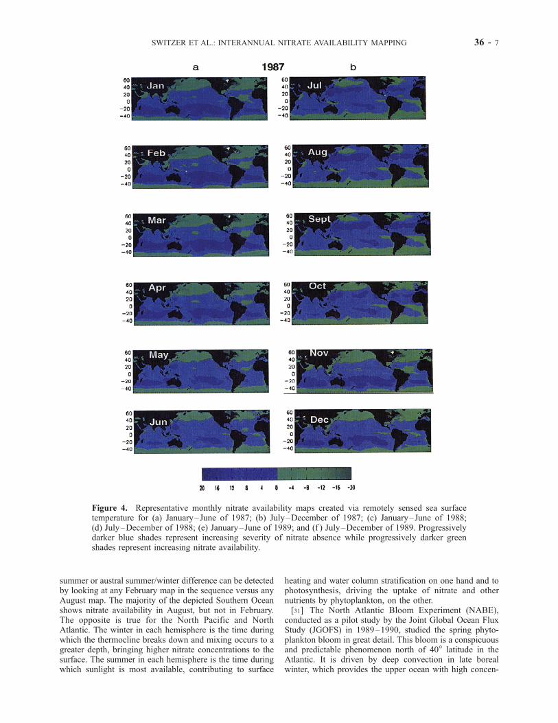
summer or austral summer/winter difference can be detectedby looking at any February map in the sequence versus anyAugust map. The majority of the depicted Southern Oceanshows nitrate availability in August, but not in February.The opposite is true for the North Pacific and NorthAtlantic. The winter in each hemisphere is the time duringwhich the thermocline breaks down and mixing occurs to agreater depth, bringing higher nitrate concentrations to thesurface. The summer in each hemisphere is the time duringwhich sunlight is most available, contributing to surface

heating and water column stratification on one hand and tophotosynthesis, driving the uptake of nitrate and othernutrients by phytoplankton, on the other.[31] The North Atlantic Bloom Experiment (NABE),

conducted as a pilot study by the Joint Global Ocean FluxStudy (JGOFS) in 1989–1990, studied the spring phyto-plankton bloom in great detail. This bloom is a conspicuousand predictable phenomenon north of 40� latitude in theAtlantic. It is driven by deep convection in late borealwinter, which provides the upper ocean with high concen-

Figure 4. Representative monthly nitrate availability maps created via remotely sensed sea surfacetemperature for (a) January–June of 1987; (b) July–December of 1987; (c) January–June of 1988;(d) July–December of 1988; (e) January–June of 1989; and (f ) July–December of 1989. Progressivelydarker blue shades represent increasing severity of nitrate absence while progressively darker greenshades represent increasing nitrate availability.

SWITZER ET AL.: INTERANNUAL NITRATE AVAILABILITY MAPPING 36 - 7

trations of nitrate. The nitrate in turn supports new produc-tion following restratification in April and May [Ducklowand Harris, 1993]. In the series of maps shown here, theeffect of these blooms can be seen as a distinct disappear-ance of nitrate in the North Atlantic in June and July ascompared to earlier boreal spring months.[32] Another area of note is the northern Indian Ocean.

Emphasizing only wind effects here, the northeast monsoon,which occurs during the boreal winter months, is charac-terized by wind that originates due to high pressure overland and thus blows toward the sea [Tchernia, 1980]. Thesewinds cause areas of upwelling in the northern Arabian Seaand Bay of Bengal. Ocean currents are influenced by thesesame offshore winds and the Coriolis force, thus the nitrate-rich areas are in the northwestern sections of these basins.

These defined upwelling zones can be seen in the Decemberthrough February months shown in Figure 4. Similarly, thesouthwest monsoon occurs in boreal summer when inten-sive warming of southern Eurasia and northern Africacreates a low pressure over land. The resulting pressuregradient is directed from sea to land, causing strong onshorewind. This southwest wind is stronger over the Arabian Seathan over the Bay of Bengal [Tchernia, 1980]. The resultantupwelling is visible in the months June–August in theArabian Sea in all 3 years in Figure 4.[33] Another prominent feature apparent in the maps are

coastal upwelling areas associated with the major boundarycurrents [Smith, 1995], specifically the California, Peru,Canary, and Benguela currents. The upwelling off Californiaoccurs in the boreal winter months and moves north through

Figure 4. (continued)

36 - 8 SWITZER ET AL.: INTERANNUAL NITRATE AVAILABILITY MAPPING

the summer in the series in Figure 4. The Peru upwelling canbe seen April–December, except in 1987 due to effects of ElNino, as already discussed. The northwest Africa upwellingcan be seen most strongly in January–May. The southwestAfrica upwelling occurs virtually year-round but is mostsignificant in the months June–November.

4. Discussion

[34] Since oceanic nitrogen is one of the most basicbuilding blocks for marine phytoplankton, these nitrate mapscan be logically related to global views of phytoplanktonchlorophyll-a provided by SeaWiFs ocean color. Thesechlorophyll-a images are created by virtue of the scatter-ing/absorption characteristics of phytoplankton in the surfacewaters [Kirk, 1986]. The nitrate availability maps created in

this study and ocean color maps should correspond to somedegree, based on the cause and effect relationship. To checkthe extent of this relationship, two averaged maps of chloro-phyll-a concentration were compared to the correspondingnitrate availability maps (Figure 5) generated using SST datafor the same time period.[35] In both February and August of 1999, there is good

agreement between nitrate availability and chlorophyll-a.The maps show that the central gyres of the Atlantic andPacific contained low values of each. There is also agree-ment of some large productive areas such as the northwest-ern North Atlantic, the southeastern tip of South America,the southwestern tip of Africa, and the Arabian Sea. How-ever, there are areas that do not seem to match well, such asthe subarctic Pacific in February. In this month, there appearsto be plenty of nitrate but low pigment, possibly due to

Figure 4. (continued)

SWITZER ET AL.: INTERANNUAL NITRATE AVAILABILITY MAPPING 36 - 9

critical depth arguments [Lalli and Parsons, 1993] and/oriron limitation [Denman and Pena, 1999]. Also, in bothmonths, there is a band of nitrate in the equatorial region ofthe Pacific which varies in strength and surface area but isdefinitely noticeable, while there is only a very smallcorresponding chlorophyll-a band. This may be attributableto the effect of low iron availability as has been studiedextensively [Archer and Johnson, 2000; Takeda, 1998;Mann and Lazier, 1996; Chisholm, 1995].[36] The view of nitrate in the world ocean, which this

remote-sensing based technique provides, is vastly differentthan the views previously available. In situ data do not exist

on large spatial and small temporal scales simultaneously.Therefore, using the Ocean Atlas [Levitus et al., 1994] maps(Figures 3d and 3c) as an example, only average conditionshave been depicted when looking at the global scale.Exploiting current remote-sensing technology and extend-ing its use based on the connections between physical andbiological processes in the ocean, the dynamic nature ofnutrients in the ocean can be illustrated.[37] Another benefit to this approach is that nutrients for

which depletion temperatures can be calculated, includingeventually nitrate, phosphate, and silicate, can be mappedon the same scale as other satellite-derived data. Much

Figure 5. Seasonally averaged nitrate availability maps and CZCS ocean color maps. The former are1987–1996 averages and the latter are 1978–1986. Note the effect in the landmasses when makingcomparisons. (left) Darkening green represents increasing nitrate availability. (right) Violet represents lowphytoplankton pigment while red represents high phytoplankton pigment. (a) January–March and April–June; (b) July–September and October–December.

36 - 10 SWITZER ET AL.: INTERANNUAL NITRATE AVAILABILITY MAPPING

discussion of nutrient limitation interactions in marineecosystems presently exists in the literature. For example,in the North Atlantic, silicate is depleted in late spring priorto nitrate, leading to a silicate limitation of diatom growth[Pondhaven et al., 1999]. Examples of locations which maybe considered phosphate limiting are listed by Gonzales-Gil[1998], including the central gyre of the North Pacific andestuaries in Australia. Kamykowski et al. [2002] provide amore complete picture of ocean fertilization by iron fromabove as well as by nitrate, phosphate, and silicate frombelow in relation to chlorophyll-a concentration andinferred phytoplankton community composition.[38] With frequently obtainable, global scale views of

nutrient availability, some of the larger-scale questionsrelated to upper ocean biogeochemical processes can beapproached in a new way. For example, the US JGOFSArabian Sea Expedition was designed to provide a carbonbudget for that area which exhibits some of the mostextreme concentrations of plant biomass observed anywherein the world ocean [Smith et al., 1998]. Nitrate concen-trations in the surface waters were collected as part of theeffort to model the carbon cycle, circulation, and biologicalproperties of the basin. However, these nitrate concentra-tions were only available along the actual cruise tracks.By utilizing the satellite-derived technique for predictingnitrate, the cruise tracks could be placed in spatial andtemporal nutrient availability context.[39] Over the last decade, much activity has been directed

toward computing new production in the ocean on largehorizontal scales. Because new production is that portion oftotal primary production in excess of local communitymetabolism [Sathyendranath et al., 1991], changes in thisquantity have a strong influence on the ability of the oceansto remove carbon from the atmosphere and deposit it on theseafloor [Watts et al., 1999] and on the upper limits ofsustainable fisheries harvest [Falkowski et al., 1998]. Exam-ples of recent efforts to compute new production fromsatellite data include those of Dugdale et al. [1989],Sathyendranath et al. [1991], Carder et al. [1999], andWatts et al. [1999]. While these models differ to variousdegrees in their approach to calculating new productionvalues, one common feature is that they would benefit fromocean color data that are supplemented with nutrient infor-mation on a scale only possible with remote sensingtechnology.[40] Areas of high fishery production, namely upwelling,

can be identified and quantified according to rate andduration using the maps created via this remote sensingtechnique. According to Wyatt [1980], upwelling rate deter-mines algal cell size while upwelling duration determinesthe amount of primary production. Locations with moderaterate and long duration produce large fisheries. In terms ofthe carbon cycle, areas of new production correspond toareas where a high percentage of carbon dioxide is drawndown from the atmosphere. Carbon dioxide is very solublein seawater and is bound with water to form carbonate andbicarbonate [Lalli and Parsons, 1993]. As this carbon isused by larger nitrate-utilizing phytoplankton, it has ahigher probability of sinking below the euphotic zone. Asthese phytoplankton are eaten by larger zooplankton, thecarbon also can be defecated as fecal pellets, followed byaccelerated sinking. Hence the uptake by phytoplankton and

the ensuing delivery to the seafloor becomes a significant‘‘sink’’ for atmospheric carbon dioxide, an important‘‘greenhouse’’ gas.

[41] Acknowledgments. We thank John Morrison, Lundie Spence,and Francesco Bignami for their help in this research. The work wassupported by NASA grant NAG56586. We would also like to acknowledgeour usage of sea surface temperature provided by the NASA PhysicalOceanography Distributed Active Archive Center at the Jet PropulsionLaboratory, California Institute of Technology as well as the ocean colordata provided by the SeaWiFS Project, NASA/Goddard Space FlightCenter, and ORBIMAGE.

ReferencesArcher, D. E., and K. Johnson, A model of the iron cycle in the ocean,Global Biogeochem. Cycles, 14, 269–279, 2000.

Azam, F., Microbial control of oceanic carbon flux: The plot thickens,Science, 280, 694–696, 1998.

Babin, M., J.-C. Thierrault, and L. Legendre, Potential utilization of tem-perature in estimating primary production from remote sensing data incoastal and estuarine waters, Estuarine Coastal Shelf Sci., 33, 559–579,1991.

Brown, J., A. Colling, D. Park, J. Phillips, D. Rothery, and J. Wright,Seawater: Its Composition, Properties and Behaviour, Pergamon, NewYork, 1989.

Carder, K. L., F. R. Chen, Z. P. Lee, S. K. Hawes, and D. Kamykowski,Semianalytic moderate-resolution imaging spectrometer algorithms forchlorophyll a and absorption with bio-optical domains based on nitrate-depletion temperatures, J. Geophys. Res., 104(C3), 5403–5421, 1999.

Chisholm, S. W., The iron hypothesis: Basic research meets environmentalpolicy, Rev. Geophys., 33, Suppl., 1277–1286, 1995.

de Baar, H. J. W., von Liebig’s law of the minimum and plankton ecology,Prog. Oceanogr., 34, 347–386, 1994.

Denman, K. L., and M. A. Pena, A coupled 1-D biological/physical modelof the northeast subarctic Pacific Ocean with iron limitation, Deep SeaRes., Part II, 46(11/12), 2877–2908, 1999.

Ducklow, H. W., and R. P. Harris, Introduction to the JGOFS North AtlanticBloom Experiment, Deep Sea Res., Part II, 40(1/2), 1–8, 1993.

Dugdale, R. C., and J. J. Goering, Uptake of new and regenerated forms ofnitrogen in primary productivity, Limnol. Oceanogr., 12, 196–206, 1967.

Dugdale, R. C., A. Morel, A. Bricaud, and F. P. Wilkerson, Modeling newproduction in upwelling centers: A case study of modeling new produc-tion from remotely-sensed temperature and color, J. Geophys. Res.,94(C12), 18,119–18,132, 1989.

Eppley, R. W., Temperature and phytoplankton growth in the sea, Fish.Bull., 70, 1063–1086, 1972.

Eppley, R. W., and B. J. Peterson, Particulate organic matter flux andplanktonic new production in the deep ocean, Nature, 282, 677–680,1979.

Falkowski, P. G., R. T. Barber, and V. Smetacek, Biogeochemical controlsand feedbacks on ocean primary production, Science, 281, 200–206,1998.

Garside, C., and J. C. Garside, Euphotic-zone algorithms for the NABE andEqPac study sites, Deep Sea Res., Part II, 42(7), 335–347, 1995.

Gonzales-Gil, S., B. A. Keafer, R. V. M. Jovine, A. Aguilera, and D. M.Anderson, Detection and quantification of alkaline phosphates in singlecells of phosphorus-starved marine phytoplankton, Mar. Ecol. Prog. Ser.,163, 21–35, 1998.

Goodberlet, M. A., C. T. Swift, K. P. Kiley, J. L. Miller, and J. B. Zaitzeff,Microwave remote sensing of coastal zone salinity, J. Coastal Res., 13(2),363–872, 1997.

Haldron, H. N., and T. A. Probyn, Nitrate supply and potential new produc-tion in the Benguela upwelling system, S. Afr. J. Mar. Sci., 12, 29–39,1992.

Harrison, W. G., Regeneration of nutrients, in Primary Productivity andBiogeochemical Cycles in the Sea, edited by P. Falkowski and W. Head,pp. 385–407, Plenum, New York, 1992.

Hutchins, D. A., and K. W. Bruland, Iron-limited diatom growth and Si:Nuptake ratios in a coastal upwelling regime, Nature, 393, 561–564, 1998.

Kamykowski, D., Some perspectives on ecological modeling focused onupper ocean processes, in Dynamic Processes in the Chemistry of theUpper Ocean, pp. 197–213, Plenum, New York, 1986.

Kamykowski, D., A preliminary biophysical model of the relationshipbetween temperature and plant nutrients in the upper ocean, Deep SeaRes., 34(7), 1067–1079, 1987.

Kamykowski, D., and S.-J. Zentara, Predicting plant nutrient concentrationsfrom temperature and sigma-t in the upper kilometer of the world ocean,Deep Sea Res., 33(1), 89–105, 1986.

SWITZER ET AL.: INTERANNUAL NITRATE AVAILABILITY MAPPING 36 - 11

Kamykowski, D., S.-J. Zentara, J. M. Morrison, and A. C. Switzer,Dynamic global patterns of nitrate, phosphate, silicate, and iron availabilityand phytoplankton community composition from remote sensing data,Global Biogeochem. Cycles, 16(4), 1077, doi:10.1029/2001GB001640,2002.

Kirk, J. T. O., Light and Photosynthesis in Aquatic Ecosystems, CambridgeUniv. Press, New York, 1986.

Lalli, C. M., and T. M. Parsons, Biological Oceanography: An Introduction,Pergamon, New York, 1993.

Legendre, L., and F. Rassoulzadegan, Plankton and nutrient dynamics inmarine waters, Ophelia, 41, 153–172, 1995.

Levitus, S., M. E. Conkright, J. L. Reid, R. G. Najjar, and A. Mantyla,Distribution of nitrate, phosphate and silicate in the world oceans, Prog.Oceanogr., 31, 245–273, 1993.

Levitus, S., R. Burgett, and T. Boyer, World Ocean Atlas 1994, vol. 3,Salinity, NOAA Atlas NESDIS 3, Natl. Oceanic and Atmos. Admin.,Silver Spring, Md., 1994.

Mann, K. H., and J. R. N. Lazier, Dynamics of Marine Ecosystems: Bio-logical-Physical Interactions in the Oceans, 2nd ed., Blackwell Sci.,Malden, Mass., 1996.

McCarthy, J. J., The kinetics of nutrient utilization, in Physiological Basesof Phytoplankton Ecology, edited by T. Platt, Can. Bull. Fish. Aquat. Sci.,210, 211–233, 1981.

Minas, H. J., and L. A. Codispoti, Estimation of primary production byobservation of changes in the mesoscale nitrate field, ICES Mar. Sci.Symp., 197, 215–235, 1993.

Morin, P., M. V. M. Wafer, and P. L. Corre, Estimation of nitrate flux in atidal front from satellite-derived temperature data, J. Geophys. Res.,98(C3), 4689–4695, 1993.

Parsons, T. R.,Y. Maita, and C. M. Lalli, A Manual of Chemical andBiological Methods for Seawater Analysis, Pergamon, New York, 1984.

Paulson, C. A., and J. J. Simpson, Irradiance measurements in the upperocean, J. Phys. Oceanogr., 7, 952–956, 1977.

Pickard, G. L., Descriptive Physical Oceanography, Pergamon, New York,1963.

Pondhaven, P., D. Ruiz-Pino, J. N. Druon, C. Fravalo, and P. Treguer,Factors controlling silicon and nitrogen biogeochemical cycles in highnutrient, low chlorophyll systems (the Southern Ocean and the NorthPacific): Comparison with a mesotrophic system (the North Atlantic),Deep Sea Res., Part I, 46, 1923–1968, 1999.

Redfield, A. C., The biological control of chemical factors in the environ-ment, Am. Sci., 46, 205–221, 1958.

Sathyendranath, S., T. Platt, E. P. W. Horne, W. G. Harrison, O. Ulloa,R. Outerbridge, and N. Hoepffner, Estimation of new production in theocean by compound remote sensing, Nature, 353, 129–133, 1991.

Schluessel, P., W. J. Emery, H. Grassl, and T. Mammen, On the skin-bulktemperature difference and its impact on satellite remote sensing of seasurface temperature, J. Geophys. Res., 95(C8), 13,341–13,356, 1990.

Selby, S. M., Standard Mathematical Tables, CRC, Boca Raton, Fla., 1965.Simpson, J. J., and T. D. Dickey, Alternative parameterizations of down-ward irradiance and their dynamical significance, J. Phys. Oceanogr., 11,876–882, 1981.

Smith, R. L., The physical processes of coastal upwelling systems, inUpwelling in the Ocean: Modern Processes and Ancient Records, editedby C. P. Summerhayes et al., pp. 39–64, John Wiley, 1995.

Smith, S. L., L. A. Codispoti, J. M. Morrison, and R. T. Barber, The 1994–1996 Arabian Sea Expedition: An integrated, interdisciplinary investiga-tion of the response of the northwestern Indian Ocean to monsoonalforcing, Deep Sea Res., Part II, 45(10/11), 1905–1915, 1998.

Strickland, J. D. H., (Ed.), The Ecology of the Plankton off La Jolla,California, in the Period April Through September, 1967, Univ. of Calif.Press, Berkeley, Calif., 1967.

Takeda, S., Influence of iron availability on nutrient consumption ratio ofdiatoms in oceanic waters, Nature, 393, 774–777, 1998.

Tchernia, P., Descriptive Regional Oceanography, Pergamon, New York,1980.

Traganza, E. D., D. A. Nestor, and A. K. McDonald, Satellite observationsof a nutrients upwelling off the coast of California, J. Geophys. Res.,85(C7), 4101–4106, 1980.

Watts, L. J., S. Sathyendranath, C. Caverhill, H. Maass, T. Platt, and N. J. P.Owens, Modeling new production in the northwest Indian Ocean region,Mar. Ecol. Prog. Ser., 183, 1–12, 1999.

Wolter, K., and M. S. Timlin, Measuring the strength of ENSO: How does1997/98 rank?, Weather, 53, 315–324, 1998.

Wyatt, T., The growth season in the sea, J. Plankton Res., 2, 81–97, 1980.Zentara, S.-J., and D. Kamykowski, Latitudinal relationships among tem-perature and selected plant nutrients along the west coast of North andSouth America, J. Mar. Res., 35(2), 321–337, 1977.

�����������������������D. Kamykowski, A. C. Switzer, and S.-J. Zentara, Department of Marine,

Earth and Atmospheric Sciences, North Carolina State University, Box1108, 1125 Jordan Hall, Raleigh, NC 27695, USA. (Dan_kamykowski@ncsu.edu; acswitze@unity.ncsu.edu)

36 - 12 SWITZER ET AL.: INTERANNUAL NITRATE AVAILABILITY MAPPING