Ar

Ya

b

c

d

a

ARA

KLLS

1

taorot1ig2aasrf

R

0d

International Journal of Applied Earth Observation and Geoinformation 17 (2012) 76–84

Contents lists available at SciVerse ScienceDirect

International Journal of Applied Earth Observation andGeoinformation

jo u rn al hom epage: www.elsev ier .com/ locate / jag

revised surface resistance parameterisation for estimating latent heat flux fromemotely sensed data

i Songa,b,∗, Jiemin Wanga, Kun Yangc, Mingguo Maa, Xin Lia, Zhihui Zhanga,d, Xufeng Wanga,d

Cold and Arid Regions Environmental and Engineering Research Institute, Chinese Academy of Sciences, Lanzhou 730000, ChinaInstitute of Earth Environment, Chinese Academy of Sciences, Xi’an 710075, ChinaInstitute of Tibetan Plateau Research, Chinese Academy of Sciences, Beijing 100085, ChinaGraduate University of Chinese Academy of Sciences, Beijing 100049, China

r t i c l e i n f o

rticle history:eceived 25 October 2010ccepted 22 October 2011

eywords:atent heat fluxandsat TM and ETM+urface resistance

a b s t r a c t

Estimating evapotranspiration (ET) is required for many environmental studies. Remote sensing providesthe ability to spatially map latent heat flux. Many studies have developed approaches to derive spatiallydistributed surface energy fluxes from various satellite sensors with the help of field observations.

In this study, remote-sensing-based �E mapping was conducted using a Landsat Thematic Mapper (TM)image and an Enhanced Thematic Mapper Plus (ETM+) image. The remotely sensed data and field obser-vations employed in this study were obtained from Watershed Allied Telemetry Experimental Research(WATER). A biophysics-based surface resistance model was revised to account for water stress and tem-perature constraints. The precision of the results was validated using ‘ground truth’ data obtained by

eddy covariance (EC) system.

Scale effects play an important role, especially for parameter optimisation and validation of the latentheat flux (�E). After considering the footprint of EC, the �E derived from the remote sensing data wascomparable to the EC measured value during the satellite’s passage. The results showed that the revisedsurface resistance parameterisation scheme was useful for estimating the latent heat flux over croplandin arid regions.

. Introduction

Evapotranspiration (ET) governs the water cycle and energyransport among the biosphere, atmosphere and hydrosphere as

controlling factor. It plays an important role in hydrology, mete-rology, and agriculture, such as in prediction and estimation ofegional-scale surface runoff and underground water, in simulationf large-scale atmospheric circulation and global climate change, inhe scheduling of field-scale field irrigations and tillage (Idso et al.,975; Z.L. Li et al., 2009; Su, 2002). Understanding the variability

n water cycle processes requires a spatially detailed analysis oflobal land surface processes (Fisher et al., 2008; Running et al.,000). Latent heat flux (�E) at a small scale can be monitored usingn eddy covariance (EC) system. However, in situ measurementsre limited for use over larger areas. Remotely sensed data from

atellites provide temporally and spatially continuous informationelated to the properties of the land surfaces, such as land sur-ace temperature (LST), leaf area index (LAI), vegetation indices

∗ Corresponding author at: Cold and Arid Regions Environmental and Engineeringesearch Institute, Chinese Academy of Sciences, Lanzhou 730000, China.

E-mail address: songyi05@sohu.com (Y. Song).

303-2434/$ – see front matter © 2011 Elsevier B.V. All rights reserved.oi:10.1016/j.jag.2011.10.011

© 2011 Elsevier B.V. All rights reserved.

and vegetation type (Huete et al., 2002; Myneni et al., 2002; Wanet al., 2002). These biophysical properties can be obtained fromimages acquired by the NOAA Advanced Very High ResolutionRadiometer (AVHRR), the MODerate Resolution Imaging Spectro-radiometer (MODIS), the Landsat Thematic Mapper (TM) and theEnhanced Thematic Mapper Plus (ETM+). There have been consid-erable efforts by the scientific community to use these remotelysensed data to estimate spatially and temporally distributed evap-oration rates, with the help of field observations (Leuning et al.,2008).

Compared with other methods of estimation based on remotelysensed data, the Penman–Monteith (P–M) equation (Monteith,1964) has been proven effective at both the point scale and kilo-metre scale (Cleugh et al., 2007; Leuning et al., 2008; Mu et al.,2007; Zhang et al., 2008). Many algorithms based on the P–M equa-tion have been developed to estimate ET at the global scale usingremotely sensed data. Cleugh et al. (2007) evaluated two models,the aerodynamic resistance–surface energy balance model and theP–M equation. The results showed that the P–M model performed

well when gridded meteorological data at coarser spatial (0.05◦)and temporal (daily) resolutions were substituted for locally mea-sured inputs. However, Cleugh et al.’s algorithm (2007) had twoproblems when it was applied to some dry or cold regions. First,

rth Ob

tria2tcoicr(ipdtrtaitita

teianHatiSomsetbtnpco

2

tisob

2

i

i�7a

ments from the heat-plate to calculate G, there was still the issueof how to estimate the soil thermal conductivity. The temperatureprediction–correction method (TDEC) presented by Yang and Wang(2008) was used to estimate G at the point scale from profiles of soil

Y. Song et al. / International Journal of Applied Ea

he model assumes that surface resistance is equal to the canopyesistance and that soil evaporation is small enough to be neglectedn comparison to transpiration from plants, but these assumptionsre only occasionally justified (Bethenod et al., 2000; Hsiao and Xu,005; Villalobos and Fereres, 1990; Wilson et al., 2000). Second,here was no water stress or temperature constraint on the canopyonductance in the algorithm, which can result in large biases in dryr cold seasons. Mu et al. (2007) developed a global remote sens-ng ET algorithm based on Cleugh et al.’s research. Their algorithmonsidered both the surface energy partitioning process and envi-onmental constraints on ET. However, the effect of soil moistureespecially the soil moisture at the rooting depth) on ET was ignoredn this algorithm. Leuning et al. (2008) introduced a simple bio-hysical model for surface conductance using remotely sensed LAIata to calculate the daily average evaporation at a kilometre spa-ial resolution. They also confirmed that the P–M equation provideseliable estimates of evaporation rates from land surfaces at dailyime scales and kilometre space scales. However, the calculation oferodynamic resistance is restricted for neutral stability conditionsn which temperature, atmospheric pressure, and wind velocity dis-ributions follow nearly adiabatic conditions. When predicting ETn the well-watered reference surface, heat exchange is small, andherefore, stability correction is normally not required. For mostrid and semi-arid regions, stability correction is needed.

Considering the limits of the above algorithms, the objective ofhis research was to improve the surface resistance model (Leuningt al., 2008) in order to estimate regional �E using Landsat TMmages at a regional scale. Two issues were addressed in our study,ccurate estimation and reasonable validation. Accurate estimationeeds an algorithm with good logic and reliable biophysical base.owever, without a reasonable validation strategy, an inequitablessessment would be made for the estimation. Therefore, both thewo issues are important in our study. The first half of this paperntroduced a revised surface resistance parameterisation we used.ubsequently, a convincing validation scheme was discussed. Inrder to show the errors in each intermediate procedure, the inter-ediate results such as the net absorbed radiation (Rn) and the

oil heat flux (G) were validated at first. In most studies, only thestimate of one pixel where the EC was located was involved inhe validation of �E. However, this validation strategy may note sufficient because the source area could cover several pixels ofhe images used for the remote-sensing-based estimation. A ratio-al validation strategy considering the source area of the EC couldrovide an equitable assessment of the estimation. Therefore, weonclude by examining the influence of two validation strategiesn the validation of the estimation.

. Data

The remotely sensed data and field observations employed inhis study were derived from Watershed Allied Telemetry Exper-mental Research (WATER). WATER is a simultaneous airborne,atellite-borne, and ground-based remote sensing experimentccurring in the Heihe River Basin, the second largest inland riverasin in the arid regions of northwest China (X. Li et al., 2009).

.1. Satellite images

The study used remotely sensed data, including a Landsat TMmage, an ETM+ image, and MODIS LAI products.

In detail, two images, including a Landsat TM image and an ETM+

mage, were involved in the remote-sensing-based estimation ofE. The Landsat TM image was acquired at 11:42 am (Beijing time),th July 2008, and the passing time of the ETM+ image was 11:45m (Beijing time), 29th June 2008. Two additional ETM+ images

servation and Geoinformation 17 (2012) 76–84 77

were involved in the estimation for this study. We had hoped touse the validation method at more time points; however, this wasprevented by the striping noise of the ETM+ images.

These two images were pre-processed using radiative, atmo-spheric and geometric correlations. For the TM and ETM+ images,the bias and gain values for each band are generally in the headerfile. For thermal bands, it is possible to convert these digital num-bers (DNs) to degrees Kelvin using a two-step process. The first stepconverts the DNs to radiance values using the bias and gain valuesspecific to the individual scene you are working with (Markham andBarker, 1986). The second step converts the radiance data to Kelvin(Schott and Volchok, 1985). Atmospheric correlation was carriedout using ENVI FLAASH. Initial visibility was 33.86 km obtained bya sun photometer (CE318).

The eight-day standard MODIS LAI products (MOD15A2), witha spatial resolution of 1 km × 1 km (Myneni et al., 2002), were usedto calculate the surface resistance.

2.2. Field observations

WATER contains 6 key stations that include an Automatic Mete-orological Station (AMS) and a Soil Moisture and TemperatureMeasuring System (SMTMS). There are an additional 6 super-stations that observe the same parameters as the key stations plusenergy and CO2 fluxes. The field observations in this study wereobtained from the Yingke (YK) oasis super-station, which includesan AMS, an EC system and a SMTMS (X. Li et al., 2009). The underly-ing surface around the YK oasis super-station is a typical irrigatedfarmland. The primary crop is seed corn (see Fig. 1). Data from1st June to 9th July were involved in parameter optimisation. Theobservations included wind speed (3 m and 10 m), air temperature(3 m and 10 m), humidity (3 m), air pressure, four components ofradiation (3 m), soil temperature and moisture profiles (measuredat depths of 10 cm, 20 cm, 40 cm, 80 cm, 120 cm, and 160 cm), andturbulent fluxes (measured at 2.81 m above the ground by the ECsystem). The four components of radiation indicate the total solarradiation, the reflective shortwave radiation, the land surface longwave radiation, and the atmospheric long wave radiation.

Measurements of soil heat flux at 15 cm depth were obtainedby a heat-plate. G can be calculated by integrating soil heat flux at15 cm depth to the surface. However, when we used the measure-

Fig. 1. Picture of environment around the Yingke station on June 2008.

78 Y. Song et al. / International Journal of Applied Earth Ob

-50

0

50

100

2008 0629 20080 70820080705

G a

t 15

cm d

epth

(W m

-2)

Date

15cm- TDEC 15cm-heat pl ate

200807 02

FJ

mtpMiTrdu

paocMpf(e(wp

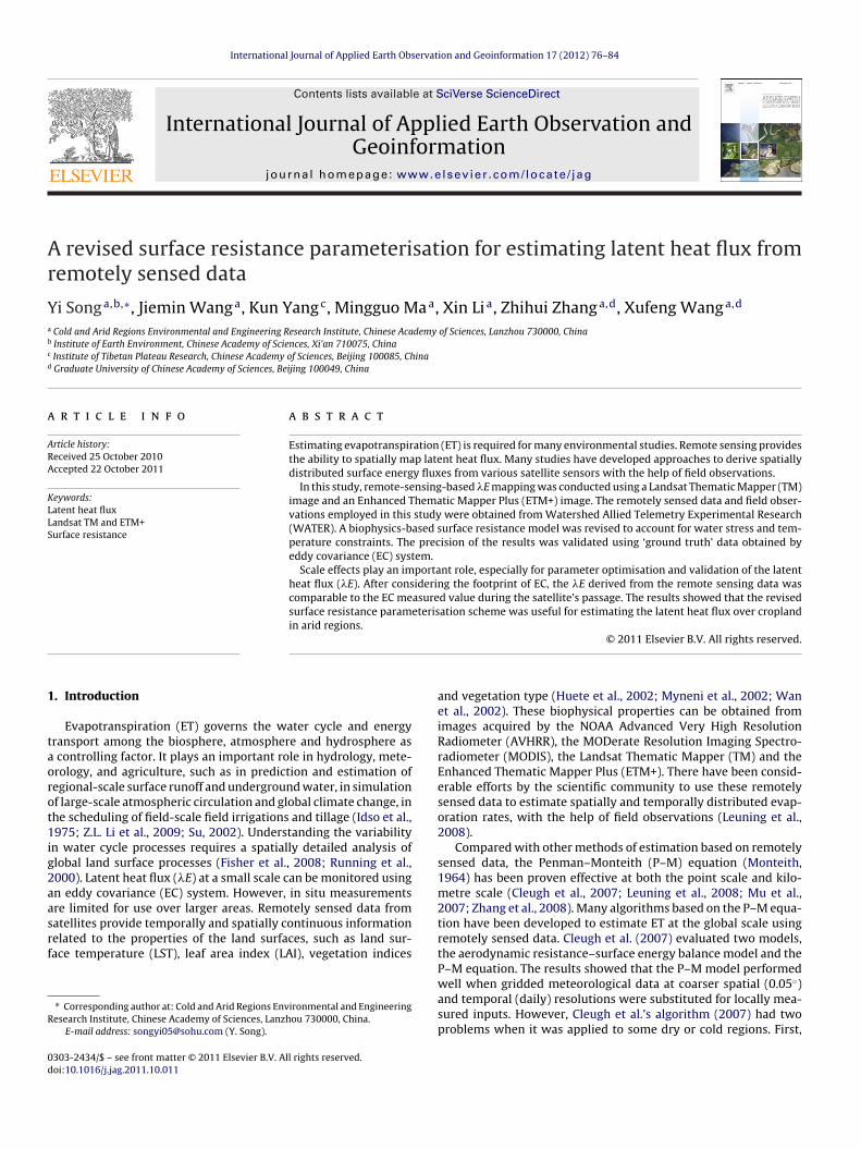
ig. 2. Observed and calculated heat flux at 15 cm depth at Yingke station from 29thune to 9th July 2008.

oisture and temperature. This method does not require accuratehermal conductivity and is not sensitive to the availability of tem-erature data in the topsoil. The profile of soil flux was obtained.easurements from the heat-plate at 15 cm were then used to val-

date the estimates using the TDEC at the same depth (see Fig. 2).he TDEC method was able to calculate the G with reliable accu-acy. Therefore, the results of the TDEC were used as ‘ground truth’ata to validate the estimate of the G from remote sensing and weresed to analyse the energy balance closure, as described below.

The raw high frequency (10 Hz) data from EC was processed toroduce half-hourly fluxes of CO2, water vapour and sensible heatbove the canopy by using post-processing software EdiRe (devel-ped by Edinburgh University, UK). The turbulent flux data werealculated from EC measurements after de-spiking (Vickers andahrt, 1997), tilt correction (Wilczak et al., 2001), sonic virtual tem-

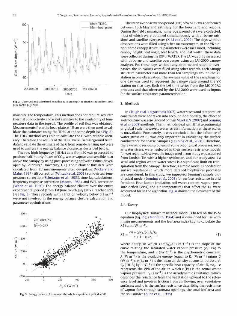
erature correction (Schotanus et al., 1983), time-lag calculations,requency response correction (Moore, 1986), and WPL correctionWebb et al., 1980). The energy balance closure over the entirexperimental period (from 1st June to 9th July) at YK reached 89%

see Fig. 3). Those records with a friction velocity below 0.1 m s−1

ere not involved in the energy balance closure calculation andarameter optimisations.

-20 0 0 20 0 40 0 60 0 80 0-20 0

0

200

400

600

800

LE+H

(W m

-2)

Rn-G (W m-2)

y=0. 889 75xR2=0.962

Fig. 3. Energy balance closure over the whole experiment period at YK.

servation and Geoinformation 17 (2012) 76–84

The intensive observation period (IOP) of WATER was performedbetween 15th May and 22th July, for the forest and arid regions.During the field campaigns, numerous ground data were collected,most of which were obtained simultaneously with airborne mis-sions and satellite overpasses (X. Li et al., 2009). The days withoutobservations were filled using other measurements. At the YK sta-tion, some canopy structure parameters were measured, includingcanopy height, leaf angle, leaf length, and leaf width; these datawere collected during the IOP of WATER. The LAI was only measuredwith airborne and satellite overpasses using an LAI-2000 canopyanalyser. For those days without any airborne and satellite over-passes, the LAI values were filled using other records. Each canopystructure parameter had more than ten samplings around the YKstation in one observation. The average value of the samplings forone day was used to represent the canopy state around the YKstation on that day. Both the LAI time series from the MOD15A2products and that observed by the LAI-2000 were used as inputsfor the surface resistance parameterisation.

3. Methods

In Cleugh et al.’s algorithm (2007), water stress and temperatureconstraints were not taken into account. Additionally, the effect ofsoil moisture was also ignored both in Mu et al.’s (2007) and Leuninget al.’s (2008) methods. Their methods deal with ET at a continentalor global scale; however, water stress information at these scalesis unavailable. Fortunately, it was concluded that the influence ofwater stress on ET was only important in calculating the surfaceconductance for sparse canopies (Leuning et al., 2008). Therefore,there were no serious problems if some biophysical processes, suchas water stress, were neglected in their surface resistance modelsfor wet regions. However, the image used in our study was acquiredfrom Landsat TM with a higher resolution, and our study area is asemi-arid region where water stress is a significant limit on tran-spiration from the canopy. Therefore, a simple model is needed forsurface resistance in which more detailed biophysical processesare considered. In this study, we improved Leuning’s simple bio-physical model (Leuning et al., 2008) for surface resistance in aridfarmland. Four factors (radiation, soil water content, vapour pres-sure deficit (VPD) and air temperature) that affect the ET wereaccounted for in the algorithm. Fig. 4 showed the flowchart of themodel.

3.1. Theory

Our biophysical surface resistance model is based on the P–Mequation (Eq. (1)) (Monteith, 1964) and is developed for use within situ measurements and the leaf area index (Lai) to calculate the�E (unit: W m−2).

�E = εA + (�cp/�)Da/ra

ε + 1 + rs/ra, (1)

where ε = s/� , in which s = d(e0)/dT (Pa ◦C−1) is the slope of thecurve relating the saturated water vapour pressure (e0: Pa) tothe temperature, and � (Pa ◦C−1) is the psychometric constant;A (W m−2) is the available energy (equal to Rn (W m−2) minus G(W m−2)); � (kg m−3) is the mean air density at constant pressure;Cp (1013 J kg−1 ◦C−1) is the specific heat capacity of air; Da = e0 − erepresents the VPD of the air, in which e (Pa) is the actual watervapour pressure; ra (s m−1) is the aerodynamic resistance, whichdescribes the resistance from the vegetation upward to the refer-

ence level and involves friction from air flowing over vegetativesurfaces; and rs is the surface resistance describing the resistanceof vapour flow through stomata openings, the total leaf area andthe soil surface (Allen et al., 1998).

Y. Song et al. / International Journal of Applied Earth Observation and Geoinformation 17 (2012) 76–84 79

g the s

t

�

eatesBts(tm�(ets

�

wifs

�

wf

R

Fig. 4. Flowchart showin

Total �E is the sum of the �Ec from the canopy and the �Es fromhe soil:

E = �Ec + �Es. (2)

The total available energy A is divided into Ac, which is thenergy absorbed by the canopy, and As, which is the energybsorbed by the soil. Evaporation from the soil occurs at a frac-ion of the equilibrium rate at the soil’s surface, εAs/(1 + ε) (Leuningt al., 2008). This fraction varies with the moisture content of theoil near the surface. Based on the complementary hypothesis ofouchet (1963), surface moisture status is linked to and reflectshe evaporative demand of the atmosphere. The assumption is thatoil moisture is reflected in the adjacent atmospheric moistureBouchet, 1963). Under convective conditions, atmospheric mois-ure has strongest link with soil moisture because of strong vertical

ixing and the influence of surface conditions on the atmosphere.Es is constrained by fSM, which is an index of the soil water deficitsee Eq. (3)) (Fisher et al., 2008). It has been proven that over largenough spatial scales, the surface tends to be in equilibrium withhe overlying atmosphere, and fSM is a good indication of surfaceoil moisture (Fisher et al., 2008):

Es = εAs

ε + 1a[fwet + fSM(1 − fwet)], (3)

here a = 1.26 (Priestley and Taylor, 1972); fwet = RH4, indicat-ng a relative surface wetness; RH is the relative humidity; andSM = RHDa/b, with b = 1000 Pa, which expresses a soil moisture con-traint.

Eq. (1) can be written as follows:

E = εAc + (�cp/�)Da/ra

ε + 1 + rc/ra+ εAs

ε + 1˛[fwet + fSM(1 − fwet)], (4)

here rc is the canopy resistance. The budget of the net radiationrom the soil and the canopy can be calculated using Beer’s law:

ns = Rn × �, (5-a)

urface resistance model.

where � is the transmissivity of the canopy estimated by the fol-lowing equation:

� = exp(

−kA × Lai

cos �

), (5-b)

where kA is an extinction coefficient for Rn related to the canopystructure, which was given a constant value during the study timeperiod; � is the solar zenith angle; Ac is equal to Rnc; and As is thedifference between Rns and G. The input of G for the surface resis-tance model was calculated from soil moisture and temperatureprofiles using the method presented by Yang and Wang (2008).

The transfer of heat and water vapour from the evaporating sur-face into the air above the canopy depends on the aerodynamicresistance as follows:

ra = [ln(z − d/zom) − �m(z − d/L)][ln(z − d/zoh) − �h(z − d/L)]k2uz

,

(7)

where z is the height of the wind and humidity measurements (m);d is the zero-plane displacement height (m); Zom is the roughnesslength governing momentum transfer (m); Zoh is the roughnesslength governing the transfer of heat and vapour (m); �m and �h arethe stability correction functions for momentum and heat respec-tively; L is the Monin–Obukhov length (m); k is the von Karman’sconstant (0.41); and uz (m s−1) is the wind speed at height z; d, Zom

and Zoh are estimated using the relations d = 2h/3, Zom = 0.123h andZoh = 0.1Zom, where h is the canopy height (Allen et al., 1998).

Under unstable conditions, the stability correction functions �m

and �h can be written as follows (Paulson, 1970):

�m = 2 ln[

1 + X]

+ ln

[1 + X2

]− 2 arctan X + 0.5, (8-a)

2 2

�h = 2 ln

[1 + X2

2

], (8-b)

80 Y. Song et al. / International Journal of Applied Earth Ob

Table 1Two groups of optimised parameters using different LAI inputs.

kA rc min (s m−1) Cv F

MODIS 1.6176 36.6431 0.0108 0.1297

N

wt

�

wm

a(

r

a

F

w

f

wtra

t

F

ws0tcea

I

F

wv

TV

Nie

LAI-2000 1.2407 96.7647 0.0103 0.1072

ote: F is the value of the cost function according to Eq. (14).

here X = [1 − 16(z − d)/L]1/4. Under stable conditions, �m is equalo �h (Webb, 1970):

m = �h = −5(z − d)L

, (8-c)

here the stability function (z − d)/L is solved using Businger’sethod (1988).The canopy resistance (rc) depends both on atmospheric factors

nd on the available water content in the soil. Noilhan and Planton1989) calculated rc as follows:

c = rc min

LaiF−1

1 F−12 F−1

3 F−44 . (9)

The factor F1 describes the influence of the photosyntheticallyctive radiation (Sellers et al., 1986) as follows:

1 = 1 + f

f + (rc min/rc max), (10-a)

ith

= 0.55R↓

s

R↓sl

× 2Lai

, (10-b)

here rc min and rc max are the minimum and maximal values ofhe canopy resistance, respectively; R↓

s is the downward shortwaveadiation; and R↓

slis a limit value of 100 W m−2 for crops (Noilhan

nd Planton, 1989).The factor F2 takes into account the effect of the water stress on

he rc (Thompson et al., 1981). F2 is given by the following:

2 =

⎧⎨⎩

1 w > wcrw − wwilt

wcr − wwiltwwilt ≤ w ≤ wcr

0 w < wwilt

, (11)

here w is the soil volumetric water content at 10 cm below theurface (m3 m−3); wcr is the field capacity, which is approximately.75 times the soil’s porosity (Thompson et al., 1981); and wwilt ishe soil moisture at a permanent wilting point of −1.5 MPa, which isommon for many herbaceous species (Lambers et al., 2008). How-ver, wwilt is higher in clay than it is in sandy soils. The wwilt valueround Yingke station was set at 0.08 m3 m−3.

The factor F3 addresses the effects of the VPD in the atmosphere.t was proposed by Jarvis (1976) and Sellers et al. (1986) as follows:

3 = 1 − Cv × VPD, (12)

here Cv is a species-dependent empirical parameter. Larger VPDalues produce smaller F3 and bigger rc values.

able 2alidation for LST, Rn and G.

ETM+ 20080629 11:45(Beijing time)

LST (K)

Rn (W m−2)

G (W m−2)

TM 20080707 11:42(Beijing time)

LST (K)

Rn (W m−2)

G (W m−2)

ote: on 29th June, we only had one LST measurement calculated using four componentsn the validation. One was calculated using four components of radiation. The other wasxperiment.

servation and Geoinformation 17 (2012) 76–84

The factor F4 represents the temperature constraint in rc. It wasproposed by Dickinson (1984) as follows:

F4 = 1 − 0.0016 × (298 − Ta)2, (13)

where Ta is the air temperature at 3 m. Because the constant isset to 298 K, which is the optimal temperature for the growth ofmany crops, F4 decreases and rc increases when the temperaturedeparts from 298 K. In addition, all transpiration ceases when thetemperature decreases below 273 K because water freezes at thistemperature.

3.2. Parameter optimisation

We obtained the optimal parameters kA, rc min and Cv in the sur-face resistance model by minimising the cost function Fcost (Eq. (14))as follows:

Fcost =∑N

j=1(�Emeas.j − �Ees.j)2

∑Nj=1(�Emeas.j − �Emeas)

2, (14)

where �Emeas.j is the jth observation of the latent heat flux measuredby the EC system at the Yingke station; �Ees.j is the jth latent heatflux estimate; �Emeas is the arithmetic mean of the measurements;and N is the number of samples. The meteorological inputs wereobtained from the Yingke AMS. The EC measurements and datapre-processing were briefly introduced in Section 2.2. The surfaceresistance was then parameterised.

3.3. Remote-sensing-based estimation

Regional net radiation (Rn) is derived from the radiation balanceequation at the thermal infrared band. It is given by the following:

Rn = (1 − ˛)R↓S + εR↓

L − εT4S , (15)

where Rn is the net radiation (W m−2); ̨ is the surface albedo esti-mated using the reflectance of bands 1, 3, 4, 5 and 7 of the LandsatTM image (Liang, 2000); R↓

S and R↓L are the downward short-wave

and long-wave radiation flux densities, respectively, measured bythe four-component net radiation sensor at the YK oasis super-station; ε, is the land surface emissivity calculated using an NDVIthreshold method (Sobrino et al., 2001); is the Stefan–Boltzmannconstant; and TS is the LST calculated using the thermal band radi-ance values from the Landsat TM based on the mono-windowalgorithm developed by Qin and Karnieli (2001). The average errorwas within 2 K (see Table 2). Here, the LAI was calculated using theTM image based on the method introduced by Ross (1976) becausethe spatial resolution of the MODIS LAI products did not match thatof the Landsat TM and ETM+.

G in our study region was calculated by the method presentedby Su (2002):

G = Rn × [�c + (1 − fc) × (�s − �c)]. (16)

Ground truth Estimate (one pixel)

299.7 298.5696 69389 98

301.4/300.9 299.6/299.1656 65446 58

of radiation. However, on 7th July 2008, two different LST observing was involved observed by a thermal infrared radiometer. Instrument was calibrated before the

Y. Song et al. / International Journal of Applied Earth Observation and Geoinformation 17 (2012) 76–84 81

0

1

2

3

4

5

6

2008070 82008062 8200806182008060 8

LAI-200 0 MODIS Landsat TM

LAI

20080529

Tf1i

FM

Dat e

Fig. 5. Comparison of MODIS LAI and observations derived from LAI-2000.

he ratios between the soil heat flux and the net radiation for theull vegetation canopy (� c) and bare soil (� s) were 0.05 (Monteith,973) and 0.315 (Kustas and Daughtry, 1989), respectively. An

nterpolation was then performed between these extreme cases

0 10 0 20 0 30 0 40 0 50 0 60 0 70 00

100

200

300

400

500

600

700a

b

LE_ca l (MOD -LA I) Linea r Fit of LE_ca l

LE_c

al (M

OD

-LA

I) (W

m-2)

LE_o bs (W m-2)

Equation y = a + b*xAdj. R-Squ 0.97748LE_cal Inter cep t 0

Slop e 0. 980

0 10 0 200 300 40 0 500 60 0 70 00

100

200

300

400

500

600

700

LE_ca l (L AI-200 0) Linea r Fit of LE_cal

LE_c

al (L

AI-

2000

) (W

m-2

)

LE_ob s (W m-2)

Equation y = a + b*xAdj. R-Squa 0.98038LE_cal Inter cep t 0

Slop e 0.998

ig. 6. Scatter plots of measurements versus estimates of �E calculated using (a)ODIS LAI and (b) observations derived from LAI-2000.

Fig. 7. Map of the �E values around the YK station at 11:42 am (Beijing time), 7thJuly 2008.

using the fractional canopy coverage, fc. The �E was then estimatedusing Rn, G and the surface resistance.

4. Results and validation

The two LAI time series (MOD15A2 products and measurementsfrom LAI-2000) have large differences (see Fig. 5). The LAI of onepixel is the average of the values for the area represented by thispixel. MOD15A2 products have a resolution of 1 km × 1 km. There-fore; MODIS would underestimate the LAI, especially in areas witha large heterogeneity of land cover types. However, the in situ mea-surements were always performed on farmland, which ignores theeffect of bare soil.

Different LAI inputs led to different optimised parameters (seeTable 1). Two groups of optimised parameters were used to esti-mate �E. As stated above, MODIS LAI has a resolution of 1 km × 1 km,which does not match the scale of the in situ observations. Thus, theparameters that were optimised using the LAI input derived fromLAI-2000 led to a better estimate (see Fig. 6).

The LAI calculated using the TM and ETM+ images has a reso-lution of 30 m × 30 m. A scale effect would exist regardless of thegroup of optimised parameters involved in a remote-sensing-basedestimation. However, the LAI value obtained by LAI-2000 and thedata from the YK AMS had the comparable scale. Therefore, an LAIinput from LAI-2000 provides a group of optimised parameterswith higher accuracy. The spatial variability of the soil moistureat 10 cm below the surface was not available. We assumed thatthe soil water content over a certain area would be homogeneousseveral days after irrigation because of lateral seepage. This hypoth-

esis was proposed based on numerous soil moisture data obtainedsimultaneously with airborne missions and satellite overpasses bya drying–weighing method. The �E around the YK station at middayreached approximately 400 W m−2 (see Fig. 7). The maximal and

82 Y. Song et al. / International Journal of Applied Earth Observation and Geoinformation 17 (2012) 76–84

Table 3Validation for �E using different methods (unit: W m−2).

Time Ground truth (EC) Estimate (one pixel) Estimate (footprint)

20080629 11:45 (Beijing time) 448

20080707 11:42 (Beijing time) 407

Fig. 8. The source area of the EC measurements of the YK station at the passing timeof (a) ETM+ and (b) TM.

479 441476 396

minimal values of the �E were 623 W m−2 and 47 W m−2, respec-tively. A large, triangular bare soil with a �E lower than 100 W m−2

was in the western area of the Yingke station. Areas with a regu-lar shape, which also had low �E, were villages. Additionally, roads(straight lines in the figure) also had low �E. Farmlands covered bymore crops had higher �E.

First, a separate validation strategy was used to validate theresults for LST, Rn and G (see Table 2). For both the TM and ETM+images, the accuracy of the estimates of LST and Rn is acceptable.However, G was overestimated. This overestimation would lead toan underestimation of A and �E in the final result.

The temporal observation of the EC represents a weighted aver-age over a source area, which is defined as the area upwind of themeasurement site contributing to the measured flux. If the spatialresolution of the estimation is 250 m × 250 m, or even lower, thesize of a pixel is larger than the source area of the EC. Validatingsuch results using direct observations of EC might be a reasonablemethod. However, to validate our estimates with a higher reso-lution of 30 m × 30 m using the above method was not sufficientbecause the source area of the EC covers several pixels at this reso-lution. It has been suggested that all pixels within the source area ofthe EC should be involved in the validation. Thus, at the beginningof the validation, calculating the footprint and source weight of anEC is necessary. Schmid’s FSAM model (Schmid, 1994) was usedto determine the source area and to calculate the source weightof the EC measurement at the time the two images were acquired(see Fig. 8). More than 80% of the areas within the source area ofthe EC were covered with seed corn. The source area was constantlychanging both in size and position, depending on the wind directionand speed and other qualities of the flow.

Table 3 provides the results of the validation using the two meth-ods. The EC measured value were 448 W m−2 and 407 W m−2 whenthe ETM+ and TM images were acquired, respectively. The esti-mates of the pixel where the EC was located were 479 W m−2 and476 W m−2. However, after considering the footprint of the EC, theweighted averages of the �E within the source area were 441 W m−2

and 396 W m−2, which were an obvious improvement. The overes-timation of G was one of the reasons for the underestimation of the�E. This result coincided with our deduction mentioned above.

5. Discussion and conclusions

Many algorithms focusing on ET estimation at a global scaleusing MODIS or AVHRR images ignored the effect of soil moisture(Cleugh et al., 2007; Leuning et al., 2008; Mu et al., 2007). In ourstudy, the resolution of the TM or ETM+ images was higher thanthat of the MODIS and AVHRR data. The simple biophysical modelfor surface resistance used in this paper, which accounts for radia-tion, soil water content, VPD and air temperature, can be used on apoint or regional scale.

Because a scale effect exists, it has been suggested that canopystructure parameters involved in the surface resistance parame-terisation should be taken at a similar observational scale with thesource area of the EC. In this study, we forced the field observations,

including canopy height and the LAI measured by the LAI-2000canopy analyser to have similar observational scales with the datathat were derived from the YK oasis station, such as air temperature,wind speed, turbulent fluxes and so on. As a result, we obtained

rth Ob

mr

vrvFiu

eto5MTos3ialidhoSowitbuwm

vebecdtapitaws(tabinwAt

tuG�ta

Y. Song et al. / International Journal of Applied Ea

ore reasonable optimised parameters to estimate the �E using aemotely sensed method.

However, it should be noted that two spatially heterogeneousariables were treated as constants in the estimations based onemotely sensed data. One was the aerodynamic resistance, whicharies according to the fluctuation in the canopy height (Colin andaivre, 2010). Some studies have examined the spatial heterogene-ty of the aerodynamic roughness length in the Heihe River Basinsing LIDAR measurements (Colin and Faivre, 2010).

Soil moisture is another spatially heterogeneous variable (Grantt al., 2010) and varies with evaporation, irrigation and precipita-ion rates. The soil moisture content of the top few centimetresf soil could be retrieved at a spatial resolution of approximately0 km (Njoku et al., 2003) using the data from the Advancedicrowave Scanning radiometer (AMSR-E) from the EOS Aqua and

erra satellites. This is considerably larger than the spatial res-lution of TM or ETM+. However, it is difficult to obtain spatialoil moisture (10 cm below the surface) with a high resolution of0 m × 30 m. In this study, the remote-sensing estimation method

s based on the hypothesis that the soil water content in a certainrea will be homogeneous several days after irrigation because ofateral seepage. This hypothesis was used because the probabil-ty distribution function of the soil moisture was undiscovered. Toesign a more practical scheme that could account for the spatialeterogeneity of soil moisture, more effective observation meth-ds for soil moisture are expected. Field observation arrays withMTMS will be set up in the Babao River Basin, a sub-watershedf the Heihe River Basin. Intensive observations of soil moistureill be carried out in the Heihe Watershed Allied Telemetry Exper-

mental Research (HiWATER), which is the follow-up experimento WATER. We anticipate that the spatial distribution or the proba-ility distribution function of the soil moisture will be determinedsing data from HiWATER. In the future, a more practical schemeill be designed to account for the spatial heterogeneity of soiloisture.During validation, we also examined the scale effect. The obser-

ation of EC represents a weighted average in a source area. Thus,stimating the footprint and source weight of EC measurementsefore validation is indispensable. A good coincidence betweenstimates of the �E and the EC measured value was obtained afteronsidering the source area of the EC. The source area of the ECepends on the wind direction and speed, and other qualities ofhe flow. The source area at the time that the ETM+ image wascquired (11:45 am, 29th June 2008) was larger than that at theassing time of the TM (11:42 am, 7th July 2008). After consider-

ng the source area of the EC, validation of the �E at the passingime of the TM improved more than when the ETM+ image wascquired. It was concluded that the larger source area of the ECould produce a larger scale effect on the validation of �E. This

tudy agreed with the results of Cleugh et al. (2007), Mu et al.2007) and Leuning et al. (2008), who suggested that the P–M equa-ion is useful for estimating evaporation at regional spatial scalesnd daily time scales. However, differences in the temporal scaleetween the estimates and the EC measured value were ignored

n our validation. A certain averaging period (normally 30 min) iseeded in data post-processing for EC observations (Foken, 2008),hereas the remotely sensed estimate is an instantaneous value.

spatially scaled match could be solved through the calculation ofhe footprint; a temporally scaled match is more difficult to obtain.

We concluded that the ignored heterogeneity of the soil mois-ure and the roughness length was one of the reasons for thencertainty in the remotely sensed estimate. The overestimation of

using the parameterised method led to the underestimation of theE. The scale effect played an important role in parameter optimisa-ion, remote-sensing-based estimation and validation. If the sourcerea of the EC was not considered in the validation, an inequitable

servation and Geoinformation 17 (2012) 76–84 83

assessment would be made for the remote-sensing-based estima-tion. Of course, research into the uncertainty of estimation based onremotely sensed data has not been thoroughly analysed. However,we demonstrated that this revised parameterisation for surfaceresistance is useful over small scales. The results of this study showthat the method proposed is reliable and can be used to estimatelatent heat flux over cropland in arid regions.

Acknowledgements

This work was supported by the CAS Action Plan for West Devel-opment Project “Watershed Airborne Telemetry ExperimentalResearch (WATER)” (Grant No. KZCX2-XB2-09-03), the KnowledgeInnovation Program of the Chinese Academy of Sciences (GrantNo. KZCX2-EW-312), National Natural Science Foundation of China(Grant No. 40875006) and the Chinese State Key Basic ResearchProject (Grant No. 2009CB421305). We also thank the editors andreviewers for their generous help in revising the paper.

References

Allen, R.G., Pereira, L., Raes, S., Smith, D., 1998. Crop Evapotranspiration – Guidelinesfor Computing Crop Water Requirements, Irrigation and Drainage Paper 61. FAO,Rome.

Bethenod, O., Katerji, N., Goujet, R., Bertolini, J.M., Rana, G., 2000. Determinationand validation of corn crop transpiration by sap flow measurement under fieldconditions. Theoretical and Applied Climatology 67, 153–160.

Bouchet, R.J., 1963. Evapotranspiration reelle et potentielle, signification climatique.International Association of Hydrological Sciences 62, 134–142.

Businger, J.A., 1988. A note on the Businger–Dyer profiles. Boundary-Layer Meteor42, 145–151.

Cleugh, H.A., Leuning, R., Mu, Q.Z., Running, S.W., 2007. Regional evaporation esti-mates from flux tower and MODIS satellite data. Remote Sensing of Environment106, 285–304.

Colin, J., Faivre, R., 2010. Aerodynamic roughness length estimation from very high-resolution imaging LIDAR observations over the Heihe basin in China. Hydrologyand Earth System Sciences 14, 2661–2669.

Dickinson, R.E., 1984. Modeling evapotranspiration for three dimensional globalclimate models. Climate Processes and Climate Sensitivity. Geophysical Mono-graph 29, 58–72.

Fisher, J.B., Tu, K.P., Baldocchi, D.D., 2008. Global estimates of the land–atmospherewater flux based on monthly AVHRR and ISLSCP-II data, validated at 16 FLUXNETsites. Remote Sensing of Environment 112, 901–919.

Foken, T., 2008. Micrometeorology. Springer, Berlin/Heidelberg, p. 308.Grant, J.P., Van de Griend, A.A., Wigneron, J.-P., Saleh, K., Panciera, R., Walker, J.P.,

2010. Influence of forest cover fraction on L-band soil moisture retrievals fromheterogeneous pixels using multi-angular observations. Remote Sensing of Envi-ronment 114, 1026–1037.

Hsiao, T., Xu, L., 2005. Evapotranspiration and Relative Contribution by the Soil andthe Plant. California Water Plan Update 2005. UC Davis.

Huete, A., Didan, K., Miura, T., Rodriguez, E.P., Gao, X., Ferreira, L.G., 2002. Overview ofthe radiometric and biophysical performance of the MODIS vegetation indices.Remote Sensing of Environment 83, 195–213.

Idso, S.B., Jackson, R.D., Reginato, R.J., 1975. Estimating evaporation: a techniqueadaptable to remote sensing. Science 189, 991–992.

Jarvis, P.G., 1976. The interpretation of the variations in leaf water potential andstomatal conductance found in canopies in the field. Philosophical Transactionsof the Royal Society B 273, 593–610.

Kustas, W.P., Daughtry, C.S.T., 1989. Estimation of the soil heat flux/net radiationratio from spectral data. Agricultural and Forest Meteorology 49, 205–223.

Lambers, H., Stuart Chapin III, F., Pons, T.L., 2008. Plant Physiological Ecology, 2ndedition. Springer Science, Business Media, LLC, New York, USA, p. 604.

Leuning, R., Zhang, Y.Q., Rajaud, A., Cleugh, H., Tu, K., 2008. A simple surface con-ductance model to estimate regional evaporation using MODIS leaf area indexand the Penman–Monteith equation. Water Resources Research 44, W10419,doi:10.1029/2007WR006562.

Li, X., Li, X.W., Li, Z.Y., Ma, M.G., Wang, J., Xiao, Q., Liu, Q., Che, T., Chen, E.X., Yan,G.J., Hu, Z.Y., Zhang, L.X., Chu, R.Z., Su, P.X., Liu, Q.H., Liu, S.M., Wang, J.D., Niu, Z.,Chen, Y., Jin, R., Wang, W.Z., Ran, Y.H., Xin, X.Z., Ren, H.Z., 2009. Watershed alliedtelemetry experimental research. Journal of Geophysical Research 114, D22103,doi:10.1029/2008JD011590.

Li, Z.L., Tang, R.L., Wan, Z.M., Bi, Y.Y., Zhou, C.H., Tang, B.H., Yan, G.J., Zhang, X.Y., 2009.A review of current methodologies for regional evapotranspiration estimationfrom remotely sensed data. Sensors 9, 3801–3853.

Liang, S.L., 2000. Narrowband to broadband conversions of land surface albedo: I

algorithms. Remote Sensing of Environment 76, 213–238.

Markham, B.L., Barker, J.L., 1986. Landsat-MSS and TM Post Calibration DynamicRanges, Atmospheric Reflectance and At-satellite Temperature. EOSAT LandsatTechnical Notes 1. Earth Observation Satellite Company, Lanham, Maryland, pp.3–8.

8 rth Ob

M

M

M

M

M

N

N

P

P

Q

R

R

S

S

4 Y. Song et al. / International Journal of Applied Ea

onteith, J.L.,1964. Evaporation and environment. The state and movement of waterin living organisms. In: Symposium of the Society of Experimental Biology, vol.19. Cambridge University Press, Cambridge, pp. 205–234.

onteith, J.L., 1973. Principles of Environmental Physics. Edward Arnold, London, p.241.

oore, C.J., 1986. Frequency response corrections for eddy correlation systems.Boundary-Layer Meteorology 37, 17–35.

u, Q.Z., Heinsch, F.A., Zhao, M.S., Running, S.W., 2007. Development of a globalevapotranspiration algorithm based on MODIS and global meteorology data.Remote Sensing of Environment 111, 519–536.

yneni, R.B., Hoffman, S., Knyazikhin, Y., Privette, J.L., Glassy, J., Tian, Y., Wang, Y.,Song, X., Zhang, Y., Smith, G.R., Lotsch, A., Friedl, M., Morisette, J.T., Votava,P., Nemani, R.R., Running, S.W., 2002. Global products of vegetation leaf areaand fraction absorbed PAR from year one of MODIS data. Remote Sensing ofEnvironment 83, 214–231.

oilhan, J., Planton, S., 1989. A simple parameterization of land surface processesfor meteorological models. Monthly Weather Review 117, 536–549.

joku, E.G., Jackson, T.J., Lakshmi, V., Chan, T.K., Nghiem, S.V., 2003. Soil moistureretrieval from AMSR-E. IEEE Transactions on Geoscience and Remote Sensing41, 215–229.

aulson, C.A., 1970. The mat hematic representation of wind speed and temperatureprofiles in the unstable atmospheric surface layer. Journal of the MeteorologicalSociety of Japan 9, 856–861.

riestley, C.H.B., Taylor, R.J., 1972. On the assessment of surface heat flux and evap-oration using large scale parameters. Monthly Weather Review 100, 81–92.

in, Z., Karnieli, A., 2001. A mono-window algorithm for retrieving land surfacetemperature from Landsat TM data and its application to the Israel-Egypt borderregion. International Journal of Remote Sensing 22 (18), 3719–3746.

unning, S.W., Thornton, P.E., Nemani, R.R., Glassy, J.M., 2000. Global terrestrial grossand net primary productivity from the Earth Observing System. In: Sala, O.E.,Jackson, R.B., Mooney, H.A., Howarth, R.W. (Eds.), Methods in Ecosystem Science.Springer-Verlag, New York.

oss, J., 1976. Radiative Transfer in Plant Communities. Vegetation and the Atmo-sphere, vol. 1. Academic Press, London, pp. 13–55.

chmid, H.P., 1994. Source areas for scalars and scalar fluxes. Boundary-Layer Mete-orology 67, 293–318.

chotanus, P., Nieuwstadt, F.T.M., DeBruin, H.A.R., 1983. Temperature measurementwith a sonic anemometer and its application to heat and moisture fluctuations.Boundary-Layer Meteorology 26, 81–93.

servation and Geoinformation 17 (2012) 76–84

Schott, J.R., Volchok, W.J., 1985. Thematic Mapper thermal infrared calibration. Pho-togrammetric Engineering and Remote Sensing 51, 1351–1357.

Sellers, P.J., Mintz, Y., Sud, Y.C., Dalcher, A., 1986. A simple biosphere model (SiB) foruse within general circulation models. Journal of the Atmospheric Sciences 43,505–531.

Sobrino, J.A., Raissouni, N., Li, Z.L., 2001. A comparative study of land surface emis-sivity retrieval from NOAA data. Remote Sensing of Environment 75, 256–266.

Su, Z.B., 2002. The Surface Energy Balance System (SEBS) for estimationof turbulent heat fluxes. Hydrology and Earth System Sciences 6 (1),85–99.

Thompson, N., Barrie, Ayles, M., 1981. The meteorological office rainfall andevaporation calculation system: MORECS. Hydrological Memorandum 45,27–306.

Vickers, D., Mahrt, L., 1997. Quality control and flux sampling problems fortower and aircraft data. Journal of Atmospheric and Oceanic Technology 14,512–526.

Villalobos, F.J., Fereres, E., 1990. Evaporation measurements beneath corn, cotton,and sunflower canopies. Agronomy Journal 82, 1153–1159.

Wan, Z., Zhang, Y., Zhang, Q., Li, Z.L., 2002. Validation of the landsurface temperatureproducts retrieved from Terra Moderate Resolution Imaging Spectroradiometerdata. Remote Sensing of Environment 83 (1–2), 163–180.

Webb, E.K., 1970. Profile relationships: the log-liner range and extension tostrong stability. Quarterly Journal of the Royal Meteorological Society 96,67–90.

Webb, E.K., Pearman, G.I., Leuning, R., 1980. Correction of the flux measurements fordensity effects due to heat and water vapour transfer. Quarterly Journal of theRoyal Meteorological Society 106, 85–100.

Wilczak, J.M., Oncley, S.P., Stage, S.A., 2001. Sonic anemometer tilt correction algo-rithms. Boundary-Layer Meteorology 99, 127–150.

Wilson, K.B., Hansonb, P.J., Baldocchi, D.D., 2000. Factors controlling evaporation andenergy partitioning beneath a deciduous forest over an annual cycle. Agriculturaland Forest Meteorology 102, 83–103.

Yang, K., Wang, J.M., 2008. A temperature prediction–correction method for esti-mating surface soil heat flux from soil temperature and moisture data. Science

in China Series D: Earth Sciences 51 (5), 721–729.

Zhang, Y.Q., Chiew, F.H.S., Zhang, L., Leuning, R., Cleugh, H.A., 2008. Estimat-ing catchment evaporation and runoff using MODIS leaf area index andthe Penman–Monteith equation. Water Resources Research 44, W10420,doi:10.1029/2007WR006563.