Super-resolution target identification from remotely sensed images using a Hopfield neural network

IEEE TRANSACTIONS ON GEOSCIENCE AND REMOTE SENSING, VOL. 39, NO. 4, APRIL 2001 781

Super-Resolution Target Identification from RemotelySensed Images Using a Hopfield Neural Network

Andrew J. Tatem, Hugh G. Lewis, Peter M. Atkinson, and Mark S. Nixon

Abstract—Fuzzy classification techniques have been developedrecently to estimate the class composition of image pixels, but theiroutput provides no indication of how these classes are distributedspatially within the instantaneous field of view represented by thepixel. As such, while the accuracy of land cover target identificationhas been improved using fuzzy classification, it remains for robusttechniques that provide better spatial representation of land coverto be developed. Such techniques could provide more accurate landcover metrics for determining social or environmental policy, forexample. The use of a Hopfield neural network to map the spa-tial distribution of classes more reliably using prior informationof pixel composition determined from fuzzy classification was in-vestigated. An approach was adopted that used the output from afuzzy classification to constrain a Hopfield neural network formu-lated as an energy minimization tool. The network converges to aminimum of an energy function, defined as a goal and several con-straints. Extracting the spatial distribution of target class compo-nents within each pixel was, therefore, formulated as a constraintsatisfaction problem with an optimal solution determined by theminimum of the energy function. This energy minimum representsa “best guess” map of the spatial distribution of class componentsin each pixel. The technique was applied to both synthetic and sim-ulated Landsat TM imagery, and the resultant maps provided anaccurate and improved representation of the land covers studied,with root mean square errors (RMSEs) for Landsat imagery of theorder of 0.09 pixels in the new fine resolution image recorded. Assuch, we show how, by using a Hopfield neural network, more accu-rate measures of land cover targets can be obtained compared withthose determined using the proportion images alone. The Hopfieldneural network used in this way represents a simple, robust, andefficient technique, and results suggest that it is a useful tool foridentifying land cover targets from remotely sensed imagery at thesubpixel scale.

Index Terms—Fuzzy image classification, Hopfield networks,image resolution, land cover, optimization methods, super-resolu-tion object detection.

I. INTRODUCTION

I NFORMATION on land cover features is required for man-agement and understanding of the environment. Accurate

identification and extraction of target land cover features is avital procedure for many areas of work, e.g., military intelli-gence, agricultural planning, and water resource management.Remote sensing has the potential to provide this information.Imagery derived from aircraft and satellite-mounted sensors

Manuscript received December 19, 1999; revised July 10, 2000. This workwas supported by EPSRC studentship 98 321 498.

A. J. Tatem, H. G. Lewis, and M. S. Nixon are with the Department of Elec-tronics and Computer Science, University of Southampton, Southampton, U.K.(e-mail: [email protected]).

P. M. Atkinson is with the Department of Geography, University ofSouthampton, Southampton, U.K.

Publisher Item Identifier S 0196-2892(01)02140-4.

have attributes that make remote sensing suitable for targetidentification, and the short orbit times of many sensors (of theorder of 3 h to 16 days) means a temporal sequence of imagescan be acquired, aiding the monitoring of specific features.Also, the large spatial coverage that can be obtained with im-agery from satellite sensors (e.g., of the order of 110 km )provides an advantage over costly and time-consuming groundsurvey. Many remote sensors measure ground reflectance ata fine spectral resolution and for most target identificationapplications, this provides sufficient information to identifyaccurately features of interest. Finally, remote sensing has thepotential to provide land cover target information at a varietyof scales (e.g., from 1 m to 1 km). These aspects maketarget identification from remotely sensed imagery attractive.However, there exist several practical limitations.

Perhaps the biggest drawback of target identification from re-motely sensed images relates to that of scale. Spatial scale is akey factor in the interpretation of remotely sensed land coverdata [1], and the information obtainable from such imagery canvary greatly depending on the spatial variation in the observedland cover and the specific terrain characteristics under consid-eration. There also exist practical limits to the level of detail thatcan be identified by each remote sensor and these limits are de-fined by the resolutions of the remote sensing system. One ofthe commonest measures of image characteristic used is spa-tial resolution, which determines the level of spatial detail de-picted in an image. This measure is a function of the instan-taneous field-of-view (IFOV) of a sensor, defined as the coneangle within which incident energy is focused on the detec-tors [2]. In turn, the IFOV leads to a ground resolution element(GRE) on the surface of the Earth (this GRE should not be con-fused with the pixel, which is the output product to which a ra-diance value is assigned).

The pixel represents the smallest element of a digital imageand has, therefore, traditionally represented a limit to the spa-tial detail obtainable in target feature extractions from remotelysensed imagery. Within remotely sensed images, a significantproportion of pixels is often of mixed land cover class composi-tion, and their presence can adversely affect the performance ofimage analysis operations [3]. The solution to the mixed pixelproblem typically centres on fuzzy classification. Subpixel classcomposition is estimated through the use of techniques suchas spectral mixture modeling [4], multilayer perceptrons [5],nearest neighbor classifiers [6], and support vector machines[7]. These approaches allow proportions of each pixel to be par-titioned between classes, and the output of these techniques gen-erally takes the form of a set of proportion images, each dis-playing the proportion of a certain class within each pixel. In

0196–2892/01$10.00 © 2001 IEEE

Authorized licensed use limited to: UNIVERSITY OF SOUTHAMPTON. Downloaded on July 1, 2009 at 09:12 from IEEE Xplore. Restrictions apply.

782 IEEE TRANSACTIONS ON GEOSCIENCE AND REMOTE SENSING, VOL. 39, NO. 4, APRIL 2001

most cases, this results in a more appropriate and informativerepresentation of targets than that produced using a hard, oneclass per-pixel classification. However, while the class compo-sition of every pixel is estimated, the spatial distribution of theseclass components within the pixel remains unknown.

The work in this paper, along with other work in the litera-ture, demonstrates that it is possible to identify land cover tar-gets at the subpixel scale (super-resolution). Fisher [3] arguesthat within remotely sensed images, the pixel can only be subdi-vided by creating repetitive information and Fig. 1 demonstratesthis argument, with the spatial resolution of a 22 pixel imagecontaining four classes (A, B, C and D) being increased to a 4

4 pixel image. The finer resolution means that all new pixelsfit within the old pixels and take the same value. However, thetechnique described in this paper suggests that the use of priorinformation allows greater precision. Such a land cover targetidentification technique potentially leads to several useful ap-plications.

1) To identify land cover targets at a fine spatial reso-lution from any remote sensing system.While sensorson satellites such as IKONOS (up to 1 m spatial resolu-tion) can provide sufficient spatial detail for accurate landcover target extraction, the cost and availability of suchdata may prohibit its use in many areas of work. By ap-plying the developed technique to cheaper, more readilyavailable data, for example SPOT HRV (up to 10 m spatialresolution) data, similar levels of accuracy for land covertarget extraction might be achieved.

2) To apply such a technique to obtain more accurateland cover metrics from remotely sensed imagery.By increasing the spatial resolution of land cover targetmaps derived from medium-resolution sensors such asthe Landsat thematic mapper (TM) or the SPOT high res-olution visible sensor, the potential exists to, for example,more accurately locate field boundaries or define areasof semi-natural vegetation. Such information would beof use in determining environmental or social policy, forexample.

3) For fine detail urban target identification. With the ad-vent of satellites such as IKONOS and Orbview, and themore common use of airborne remote sensing, imagery ofspatial resolution less than 5 m is becoming widely avail-able. Application of a technique to produce super-reso-lution maps of land cover targets from these source datawould allow urban land cover target extraction and map-ping of an unprecedented fine detail from remotely sensedimagery.

4) To simulate fine spatial resolution imagery from im-agery of a coarser spatial resolution.Such an approachcould aid decision making on future choices of imagery.

A. Previous Work

Only recently has research been undertaken on the subject ofidentifying land cover targets from remotely sensed images atthe subpixel scale. Schneider [8] introduced a knowledge-basedanalysis technique for the automatic localization of field bound-aries with subpixel accuracy. The technique relies on knowledge

Fig. 1. Example of Fisher’s argument.

of straight boundary features within Landsat TM scenes, andserves as a preprocessing step prior to automatic pixel-by-pixelland cover classification. With knowledge of pure pixel valueseither side of a boundary, a model is defined for each 3 by 3block of pixels, the model then uses parameters such as purepixel values, boundary angle, and distance of boundary fromthe centre pixel. Using least squares adjustment, the most ap-propriate parameters are chosen to locate a subpixel boundarythat divides mixed pixels into their respective pure components.Improvements on this technique were described in [9] whichused a neural network to speed up processing and [10], [11] and[12] put forward algorithmic improvements, along with the ad-dition of a vector segmentation step. The technique representsa successful, automated and simplistic pre-processing step forincreasing the spatial resolution of satellite imagery. However,its application is limited to features with straight boundaries ata certain spatial resolution and the models used still have prob-lems resolving image pixels containing more than two classes[13].

Flack et al. [14] also concentrated on super-resolution targetidentification at the borders of agricultural fields, where pixelsof mixed class composition occur. Edge detection and segmen-tation techniques were used to identify field boundaries and theHough transform [15] was applied to identify the straight, sub-pixel boundaries. These vector boundaries were superimposedon a subsampled version of the image, and the mixed pixels werereassigned each side of the boundaries. By altering the imagesubsampling, the degree to which the spatial resolution was in-creased could be controlled. However, no validation or furtherwork was carried out, and so the success of the technique re-mains unclear.

Aplin et al. [16] also made use of subpixel scale vectorboundary information, along with fine resolution satellitesensor imagery to identify land cover targets. By utilizing Ord-nance Survey land line vector data and undertaking per-fieldrather than the traditional per-pixel land cover classification,target identification at a subpixel scale was demonstrated. As-sessments suggested that the per-field classification techniquewas generally more accurate than the per-pixel classification.However, in most cases around the world, accurate vector datasets with which to apply the approach will rarely be available.

The techniques described so far are based on direct pro-cessing of the raw imagery. Other work has focused on usinga preprocessing step where fuzzy classification of the imageryis undertaken, and an attempt to map the location of classcomponents within the pixels is made.


TATEM et al.: SUPER-RESOLUTION TARGET IDENTIFICATION 783

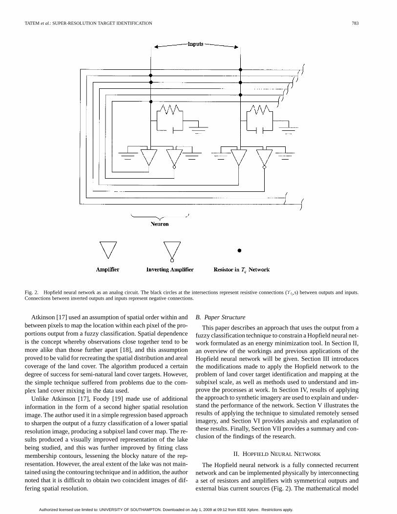
Fig. 2. Hopfield neural network as an analog circuit. The black circles at the intersections represent resistive connections (T s) between outputs and inputs.Connections between inverted outputs and inputs represent negative connections.

Atkinson [17] used an assumption of spatial order within andbetween pixels to map the location within each pixel of the pro-portions output from a fuzzy classification. Spatial dependenceis the concept whereby observations close together tend to bemore alike than those further apart [18], and this assumptionproved to be valid for recreating the spatial distribution and arealcoverage of the land cover. The algorithm produced a certaindegree of success for semi-natural land cover targets. However,the simple technique suffered from problems due to the com-plex land cover mixing in the data used.

Unlike Atkinson [17], Foody [19] made use of additionalinformation in the form of a second higher spatial resolutionimage. The author used it in a simple regression based approachto sharpen the output of a fuzzy classification of a lower spatialresolution image, producing a subpixel land cover map. The re-sults produced a visually improved representation of the lakebeing studied, and this was further improved by fitting classmembership contours, lessening the blocky nature of the rep-resentation. However, the areal extent of the lake was not main-tained using the contouring technique and in addition, the authornoted that it is difficult to obtain two coincident images of dif-fering spatial resolution.

B. Paper Structure

This paper describes an approach that uses the output from afuzzy classification technique to constrain a Hopfield neural net-work formulated as an energy minimization tool. In Section II,an overview of the workings and previous applications of theHopfield neural network will be given. Section III introducesthe modifications made to apply the Hopfield network to theproblem of land cover target identification and mapping at thesubpixel scale, as well as methods used to understand and im-prove the processes at work. In Section IV, results of applyingthe approach to synthetic imagery are used to explain and under-stand the performance of the network. Section V illustrates theresults of applying the technique to simulated remotely sensedimagery, and Section VI provides analysis and explanation ofthese results. Finally, Section VII provides a summary and con-clusion of the findings of the research.

II. HOPFIELD NEURAL NETWORK

The Hopfield neural network is a fully connected recurrentnetwork and can be implemented physically by interconnectinga set of resistors and amplifiers with symmetrical outputs andexternal bias current sources (Fig. 2). The mathematical model



describing the behavior of such an array of electronic compo-nents can be derived from Kirchoff’s current law [20], [21]

(1)

where

(2)

is the resistance between the output of amplifierand inputof amplifier, is the number of amplifiers, 0 is thecapacitance of amplifier, is the internal voltage of amplifier, and is the external bias on amplifier. is the conductance

from amplifier to amplifier , where

(3)

and is the output voltage of amplifier. is thenonlinear activation function, defined as

(4)

where determines the steepness of the function.Hopfield [22] shows how (1) can be written in a neural con-

text for ease of interpretation, where, in this case the nonlinearamplifiers correspond to neurons

(5)

wheretime constant for neuron;total weighted input at neuron ;number of neurons in the network;neural output which is a function of the input;external bias on neuron;weight from neuron to neuron .

which corresponds to the conductance in (1).The set of differential equations described so far defines the

time evolution of the network. Thus, from a set of initial neuronoutputs, the state of the network varies with time until con-vergence to a stable state, where neuron output stops varyingwith time. Weights and biases determine the neural outputs atthis stable state.

Hopfield [22] showed that using symmetric weights with noself connection, i.e., and 0 is sufficient to guar-antee convergence to such a stable state. Therefore, indepen-dent of its initial status, a Hopfield neural network will alwaysreach an equilibrium state where no output variation occurs andit was also demonstrated that for high values of the gain,, theactivation function (4) approaches a step function. The

stable states of the network consequently correspond to the localminima of the following energy function [21]:

(6)

where is the energy calculated over the whole network. Forneurons where 0 and with high values of , the last termbecomes small and can be neglected, such that

(7)

From (5) and (7), the equation describing the dynamics, i.e., therate of change of neuron input of the Hopfield network can bewritten as

(8)

or

(9)

The Hopfield network can therefore be used for energy mini-mization problems if the weights and biases are arranged suchthat they describe an energy function, with the minimum of en-ergy occurring at the stable state of the network [20]. By speci-fying different values for the weights and biases, any hypothet-ical energy minimization problem can be simulated.

Many real world problems can be formulated as the mini-mization of an energy function, and this is central to the designof a Hopfield neural network formulated as an optimization tool.The energy function used must represent the problem correctly,and reach a minimum at the solution of the problem. Once thisfunction is designed, the weights and biases can be set, and thenetwork is built around these.

Most real world problems contain built-in constraints in ad-dition to a goal that must be considered. These constraints forma cost added to the objective within the energy function, whichcan then be defined as

Energy Goal Constraints (10)

If the energy function is arranged in this particular way, the con-straints become part of the minimization process, which meansthat the constraints do not need to be treated separately, justweighted by their importance to the problem. The Hopfield net-work process then finds the minimum energy that represents acompromise between the goal and the constraints.

The Hopfield network has been used within the field of re-mote sensing for ice mapping, cloud motion, and ocean currenttracking [23], [24]. These demonstrate the utility of the Hop-field network for feature tracking, the basic principle of which



Fig. 3. (a) 2� 2 pixel image,p andq represent the image dimensions,x andy represent the image pixel coordinates. (b) Representation of the Hopfield networkfor the image in (a).i andj represent the neuron coordinates (int = integer value).

is to match common features in a sequence of images. In addi-tion, more general feature matching problems have been tackledusing a Hopfield network [25]–[27], as well as applications suchas recognition or classification [28], [29].

Hopfield and Tank [20] also used the network’s energyminimization capability and demonstrated solutions to com-plex combinatorial problems such as the traveling salesmanproblem. Hopfield and Tank formulated the problem as theminimization of an energy function, and for a ten-city problem,achieved convergence to a valid tour with an 80% success rate.Later, work in [30] and [31] eliminated the presence of localminima in the energy functions where constraints were notsatisfied by setting various constants in a certain arrangement,and this guaranteed convergence to a valid solution.

III. U SING THE HOPFIELD NEURAL NETWORK FORTARGET

IDENTIFICATION AT THE SUBPIXEL SCALE

The input data for the research described in this paper werederived from aerial photography, whereby targets were identi-fied and extracted accurately from the photographs by hand,using field survey for verification. By degrading these verifi-cation images of clearly defined land cover targets to the spatialresolution of Landsat TM data using a square mean filter, ac-curate class proportion estimates were obtained for each pixel.These provided the input to the network, but in practice, thisinput could come from automated fuzzy classification methodssuch as the multilayer perceptron. However, for the research inthis paper, the aim was to understand and test the capabilities ofthe Hopfield network technique, so any error introduced to theinput data by an automated fuzzy classification method wouldbe detrimental to this aim.

Mapping the spatial distribution of the class componentswithin each pixel was formulated as a constraint satisfactionproblem, and an optimal solution to this problem was de-termined by the minimum of an energy function coded intoa Hopfield neural network. The network architecture wasarranged to represent a finer spatial resolution image, andconstraints within the energy function determined the spatiallayout of binary neuron activations within this arrangement.The Hopfield neural network was used to find the minimum ofthe energy function, which corresponded to a bipolar map ofclass components within each pixel and this method is outlinedin detail in the following sections.

A. Network Architecture

In many papers, on the use of Hopfield neural networksfor optimization, the spatial relations between neurons areconsidered irrelevant. However, for this paper, the nature ofthe problem and the proposed solution requires the networkneurons to be considered as being arranged in a regular grid,with positioning within this grid being of significance to thenetwork design for this task (Fig. 3). Therefore, neurons will bereferred to by coordinate notation, for example, neuronrefers to a neuron in row and column of the grid and hasan input voltage of and an output voltage of . The zoomfactor determines the increase in spatial resolution from theoriginal satellite sensor image to the new high-resolution imageand after convergence to a stable state, the neurons representa bipolar classification of the land cover targetat the higherspatial resolution. Fig. 3 shows the notation used in this paperand how coordinates are transformed linearly from the imagespace to the network neuron space, for example, the pixel ()in the satellite image is represented by neurons centredat coordinates [ int int ], whereint is theinteger value.

B. Network Initialization

Each neuron is initialized with a starting value , and twostrategies for initializing the network exist.

1) Each set of neurons representing a pixel in the low-res-olution image is identified and a proportion of this setis randomly given an output of 0.55. This pro-portion is equal to the actual area proportion of the classwithin the image pixel and the remaining neurons of theset are given an output of 0.45. The values of 0.55and 0.45 were chosen as the initial on and off outputs tospeed up processing time and avoid unnecessary bias to-ward certain energy minimization paths. In [20] and manyother papers related to the use of the Hopfield networkfor solving the traveling salesman problem, neurons areinitialized with a random value close to the central statevalue (0.5). This choice is justified by the fact that no ini-tial preference should be given to any path. The small dif-ference between the two values also enables the networkto “push” neuron outputs to 1 or 0 to represent a bipolar



classification faster than if, for example, a neuron was ini-tially given an output of 0 and had to be pushed to 1 toproduce an optimal solution.

2) The completely random initialization of neuron outputswithin the range [0.45, 0.55]. This allows perfor-mance comparison with the class proportion-defined ini-tialization, and does not introduce any possible unneces-sary bias into the result, which may occur using 1), shouldestimated class proportions be inaccurate.

C. Implementation

When implemented on a digital computer, sets of biases andweights do not need to be determined, as the network is simu-lated via its equation of motion (9) using the Euler method

(11)

where is the time step of the iterative method and the functionis measured using . Equation (8) shows the

correspondence between the two functions, and is de-termined using the goals and constraint of the super-resolutiontarget identification task. Equation (11) is run until

, where is a sufficiently small value, andthe equations of motion were defined as

(12)

Each component of (12) is described in the subsequent sections.

D. The Energy Function

The goal and constraints of the subpixel mapping task weredefined such that the network energy function was

(13)

whereand constants weighting the various energy pa-

rameters;and output values for neuron of the two

objective (or goal) functions (see Sec-tion III-D1), and these correspond to thequadratic term in (5);output value for neuron of the propor-tion constraint (see Section III-D1), whichcorresponds to the linear term in (7).

1) Goal Functions: The goal (objective) functions werebased upon an assumption of spatial order [18]. Almost allnatural and human-made phenomena exhibit spatial continuityat some scale, such that points near to each other are more alikethan those further apart, and the degree of dissimilarity dependson both the environment and the nature of our observations[32]. These observations can be the pixels in remotely sensedimages, and the assumption of spatial order can be used to inferrelationships between these pixels. By focusing within thisresearch on discrete land cover targets, which all exhibit spatialorder to some degree, the assumption of spatial order becomes

particularly relevant. Therefore, by devising simple measuresof spatial order and incorporating each as objective functionswithin the Hopfield network, to map the spatial distribution ofclass components within a pixel, this real world phenomenonwas modeled.

In this case, the aim of the goal was to make the output ofa neuron similar to that of its neighboring neurons. Therefore,if the output of neuron ( ) was similar to the average outputof the eight neighboring neurons, then a low energy is given.If it is different, then this represents an undesirable situation interms of the aim of spatial order, and a high energy is produced.However, to produce a bipolar image, a function that just drivesa neuron output to be similar to the surrounding neuron outputis insufficient. Consequently, two objective functions were in-troduced, one to increase neuron output toward a value of 1 andanother to decrease neuron output to 0, each dependent on theaverage output of the eight neighboring neurons.

The first function aimed to increase the output of the centreneuron to 1 if the average output of the surrounding eightneurons was greater than 0.5

(14)

where is a gain which controls the steepness of thetanhfunc-tion. The tanh function controls the effect of the neighboringneurons. If the averaged output of the neighboring neurons isless than 0.5, then (14) evaluates to 0, and the function has no ef-fect on the energy function (13). If the averaged output is greaterthan 0.5, (14) evaluates to 1, and the function controlsthe magnitude of the negative gradient output, with onlyproducing a zero gradient. A negative gradient is required to in-crease neuron output.

The second goal function aimed to decrease the output of thecentre neuron to 0, given that the average output ofthe surrounding eight neurons was

less than 0.5

(15)

This time, thetanh function evaluates to 0 if the averagedoutput of the neighboring neurons is more than 0.5. If it isless than 0.5, the function evaluates to 1 and the center neuronoutput controls the magnitude of the positive gradientoutput, with only 0 producing a zero gradient. A positivegradient is required to decrease neuron output only when1 and , or 0 and

0.5 is the energy gradient equal

to zero, and 0. This satisfies the objective of



recreating spatial order, while also forcing neuron output toeither 1 or 0 to produce a bipolar image.

2) Proportion Constraint: While the goal functions providethe enforcement of spatial order, the sole use of these func-tions would result in all neuron outputs taking the values 1 or 0.Therefore, a method of constraining the effect of those functionsto the correct image areas was required. The proportion con-straint aimed at retaining the pixel class proportions outputfrom the fuzzy classification. This was achieved by adding inthe constraint that the total output from the set of neurons rep-resenting each coarse resolution image pixel should be equal tothe predicted class proportion for that pixel. An area proportionestimate representing the proportion of neurons with an outputof 0.55 or higher was calculated for all the neurons representingpixel

Area Proportion Estimate

(16)

The use of thetanh function ensures that if a neuron output isabove 0.55, it is counted as having an output of 1 within theestimation of class area per pixel. Below an output of 0.55, theneuron is not counted within the estimation, which simplifies thearea proportion estimation procedure and ensures that neuronoutput must exceed the random initial assignment output of 0.55in order to be counted within the calculations.

To ensure that the class proportions per pixel output from thefuzzy classification were maintained, the proportion target perpixel was subtracted from the area proportion estimate (16)

(17)

If the area proportion estimate for pixel is lower thanthe target area, a negative gradient is produced that correspondsto an increase in neuron output to counteract this problem. Anoverestimation of class area results in a positive gradient, pro-ducing a decrease in neuron output. Only when the area propor-tion estimate is identical to the target area proportion for eachpixel does a zero gradient occur, corresponding to 0 inthe energy function (13).

E. Technique Advantages

The approach described in this paper holds several strategicadvantages over those techniques mentioned in Section I-A.

• The option to choose the level of spatial resolution in-crease. This is essential if simulation of higher spatial res-olution imagery is the aim.

• The Hopfield network technique has the ability to simulateany shape rather than being restricted to straight bound-aries.

• The ease with which any additional information can beincorporated within the framework to aid the target identi-fication. Any prior information about the land cover targetdepicted in the input imagery can be coded easily into the

Hopfield network as an extra constraint to increase accu-racy.

• The design of the Hopfield network as an optimizationtool means that all constraints are satisfied simultaneously,rather than employing a multistage operation.

• The effect that each one of these constraints has onthe final prediction image can be controlled simply viaweightings.

• While the incorporation of prior information on each landcover target may increase map accuracy, the Hopfield net-work technique has the benefit of being able to produce ac-curate, super-resolution land cover target maps from justclass proportions. There is therefore no reliance on theavailability of finer spatial resolution imagery or land linevector data.

IV. I NTERPRETATION

To understand and illustrate the workings of the Hopfieldnetwork set up in this way, several synthetic images werecreated. Traditionally, within the remote sensing community,there has been a reluctance to use synthetic imagery, with theapplication of techniques directly to real imagery being pre-ferred. However, by breaking down the elements of real-worldimagery into simplified representations, understanding animage processing technique and, in turn, making improvementsto it becomes easier.

The spatial order exhibited in all natural and human-madelandscapes is demonstrated by the fact that scenes within re-motely sensed imagery are composed of various shapes, for ex-ample, fields, roads and houses. The variety of the spatial orderof shapes can be characterized using compactness and circu-larity. Compactness is defined as

(18)

where is the perimeter length, andis the area of the shape.Circularity is defined as

(19)

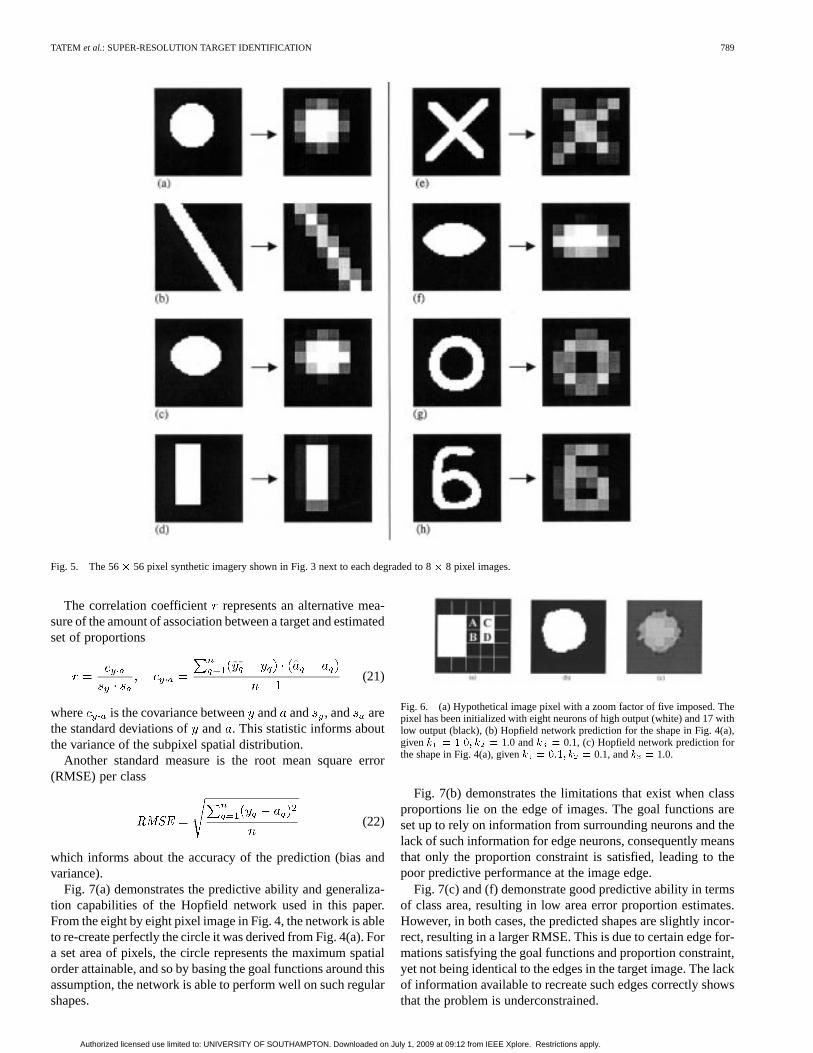
where is the area of the shape, and max is the maximum dis-tance from the shape centre to the perimeter. Fig. 4 shows eight,56 56 pixel, synthetic images of differing shapes, with theirrespective compactness and circularity measures. The shapesrepresent extremes of spatial order as well as possible landcover targets, for example (b) a road and (d) a field. In addition,the shapes cover a wide range of compactness and circularityvalues, providing a useful test of the generalization capabilitiesof the Hopfield network. Fig. 5 shows each synthetic imagesubsampled (using a 7 7 mean filter) to generate an 8 8pixel image, which causes mixing of the two classes (whiteand black) at the shape boundaries, producing eight proportionimages and imitating the effect of class mixing within remotelysensed imagery. By using these eight proportion images asinputs to the Hopfield network and setting a zoom factor of 7,it should be possible to test the capabilities of the network byapproximating the eight images each was derived from.



Fig. 4. Synthetic images and the features of the shapes depicted in each.

A. Setting the Constraint Weightings

To attempt to make predictions from the synthetic imagery,optimum values of goal and constraint weightings and

should be used, as these constants are of great importancebecause they control the direction of the optimization process.For this paper, equal weightings of 1.0 were chosen and thejustification for this decision becomes clear with the followingexamples.

Fig. 6(a) shows a hypothetical situation of an image pixel witha zoom factor of five. It should be noted that for this example,the effect of proportions within surrounding pixels is ignored forsimplicity, but in practice, the distribution of class proportionswithin the surrounding pixels may have a significant effect onthe resulting neuron activations predicted.

The target class proportion is 8/25, and using the constrainedrandom initialization method, this is satisfied immediately (ofthe 25 neurons, eight are activated). While the proportion con-straint value is zero, the goal function values for this arrange-ment and are large due to the isolated outputs of neuronsC and D. To minimize 1 and 2 and keep the target propor-tion of 8/25, neurons A and B should have an increased output,while the outputs of C and D should be reduced.

If the proportion constraint is strongly weighted, then the ar-rangement of neural outputs displayed in Fig. 6(a) remains, asis minimized, and the goal functions are not weighted stronglyenough to have an effect, i.e., .

If the goal functions are strongly weighted, then neurons Aand B display increased output, neurons C and D stay at a highoutput, and other neurons around these also increase in output.In such a case, the proportion constraint is not sufficiently strongto maintain target class proportions, i.e., .

The effect of such biased weightings is demonstrated by run-ning the network with a zoom factor of 7, for 10 000 iterationson the synthetic image in Fig. 5(a). Fig. 6(b) demonstrates thatthe predicted shape is too large and irregular without the pro-portion constraint to control the positive activation effect of thegoal functions. Giving a large weight means that maintainingtarget class proportions becomes a priority, and the goal func-tions have little effect, such that the image in Fig. 6(c) is pro-duced with a range of outputs.

By weighting the goal functions and proportion constraintequally, i.e., , each affects and controls the other tominimize the overall energy of the network, and this is demon-strated in the following examples.

B. Predictive Ability and Limitations

The results of the Hopfield network predictions from the syn-thetic imagery after 10 000 iterations, using values of 1.0 for

and are shown in Fig. 7. Three measures of accuracywere calculated to assess the difference between each networkprediction and the target images. One of the simplest measuresof agreement between a set of known proportions, and a set ofestimated proportions is the area error proportion (AEP) perclass

AEP (20)

where is the total number of neurons. This statistic informsabout bias in the prediction, and as it is based solely on areapredictions, it represents a measure of the success of the pro-portion constraint in maintaining the target proportions.



Fig. 5. The 56� 56 pixel synthetic imagery shown in Fig. 3 next to each degraded to 8� 8 pixel images.

The correlation coefficient represents an alternative mea-sure of the amount of association between a target and estimatedset of proportions

(21)

where is the covariance betweenand and , and arethe standard deviations ofand . This statistic informs aboutthe variance of the subpixel spatial distribution.

Another standard measure is the root mean square error(RMSE) per class

RMSE (22)

which informs about the accuracy of the prediction (bias andvariance).

Fig. 7(a) demonstrates the predictive ability and generaliza-tion capabilities of the Hopfield network used in this paper.From the eight by eight pixel image in Fig. 4, the network is ableto re-create perfectly the circle it was derived from Fig. 4(a). Fora set area of pixels, the circle represents the maximum spatialorder attainable, and so by basing the goal functions around thisassumption, the network is able to perform well on such regularshapes.

Fig. 6. (a) Hypothetical image pixel with a zoom factor of five imposed. Thepixel has been initialized with eight neurons of high output (white) and 17 withlow output (black), (b) Hopfield network prediction for the shape in Fig. 4(a),givenk = 1:0; k = 1.0 andk = 0.1, (c) Hopfield network prediction forthe shape in Fig. 4(a), givenk = 0:1; k = 0.1, andk = 1.0.

Fig. 7(b) demonstrates the limitations that exist when classproportions lie on the edge of images. The goal functions areset up to rely on information from surrounding neurons and thelack of such information for edge neurons, consequently meansthat only the proportion constraint is satisfied, leading to thepoor predictive performance at the image edge.

Fig. 7(c) and (f) demonstrate good predictive ability in termsof class area, resulting in low area error proportion estimates.However, in both cases, the predicted shapes are slightly incor-rect, resulting in a larger RMSE. This is due to certain edge for-mations satisfying the goal functions and proportion constraint,yet not being identical to the edges in the target image. The lackof information available to recreate such edges correctly showsthat the problem is underconstrained.



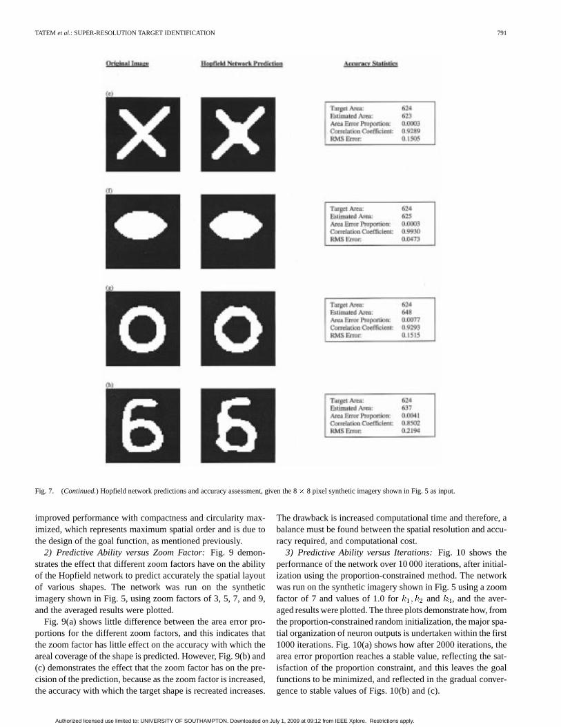
Fig. 7. Hopfield network predictions and accuracy assessment, given the 8� 8 pixel synthetic imagery shown in Fig. 5 as input.

Fig. 7(d) reflects this problem further because, as describedpreviously, the use of spatial order as the basis for the goal func-tions, means that the network will almost always converge tocurved rather than sharp corners. Unless prior knowledge existson the type of shapes that the network is aiming to recreate, thisproblem will remain.

Finally, Figs. 7(e), (g), and (h) demonstrate the ability of thenetwork to cope with more complex shapes. Comparison of,for example, Figs. 7(e) with (f) shows identical area error pro-portion values of 0.0003, demonstrating how the class area hasbeen predicted accurately. However, the correlation coefficientsand RMS errors are significantly different, representing the dif-ficulty in predicting the spatial distribution of class componentsfor a complex shape such as that in Fig. 7(e). While the propor-tion constraint has ensured that class area is maintained, withoutprior information on the shape depicted in the input proportions,the goal functions on their own are insufficient to recreate accu-rately the spatial layout of the cross.

By repeating the network run on the more complex input pro-portions in Figs. 7(e), (g), and (h), slightly different predictionsare produced each time. The use of an initialization techniquebased on random neuron output, constrained by target class pro-portions, means that starting neuron arrangements from certainnetwork runs produce lower energy than others. This results indifferent paths of convergence along the energy surface of thenetwork, and in turn, for the more complex shapes, this resultsin slightly different predictions each time, again indicating theunderconstrained nature of the problem.

1) Predictive Ability versus Shape Type:Relationships canbe drawn between the shape characteristics and the predictiveability of the network. These have the potential to be used toobtain a network performance prediction, providing that a cer-tain degree of knowledge about the input land cover shapes isknown.

Figs. 8(a) and (b) show the relationship between the var-ious shape characteristics and the RMSE. The plots suggest



Fig. 7. (Continued.) Hopfield network predictions and accuracy assessment, given the 8� 8 pixel synthetic imagery shown in Fig. 5 as input.

improved performance with compactness and circularity max-imized, which represents maximum spatial order and is due tothe design of the goal function, as mentioned previously.

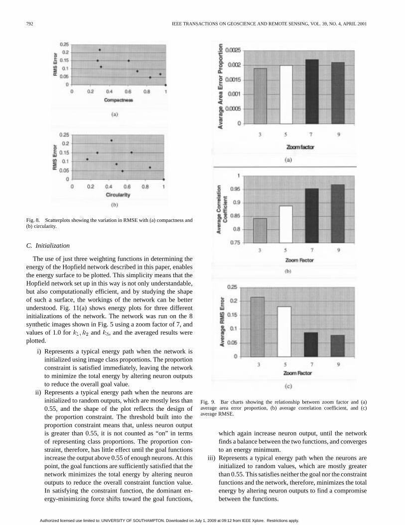
2) Predictive Ability versus Zoom Factor:Fig. 9 demon-strates the effect that different zoom factors have on the abilityof the Hopfield network to predict accurately the spatial layoutof various shapes. The network was run on the syntheticimagery shown in Fig. 5, using zoom factors of 3, 5, 7, and 9,and the averaged results were plotted.

Fig. 9(a) shows little difference between the area error pro-portions for the different zoom factors, and this indicates thatthe zoom factor has little effect on the accuracy with which theareal coverage of the shape is predicted. However, Fig. 9(b) and(c) demonstrates the effect that the zoom factor has on the pre-cision of the prediction, because as the zoom factor is increased,the accuracy with which the target shape is recreated increases.

The drawback is increased computational time and therefore, abalance must be found between the spatial resolution and accu-racy required, and computational cost.

3) Predictive Ability versus Iterations:Fig. 10 shows theperformance of the network over 10 000 iterations, after initial-ization using the proportion-constrained method. The networkwas run on the synthetic imagery shown in Fig. 5 using a zoomfactor of 7 and values of 1.0 for and , and the aver-aged results were plotted. The three plots demonstrate how, fromthe proportion-constrained random initialization, the major spa-tial organization of neuron outputs is undertaken within the first1000 iterations. Fig. 10(a) shows how after 2000 iterations, thearea error proportion reaches a stable value, reflecting the sat-isfaction of the proportion constraint, and this leaves the goalfunctions to be minimized, and reflected in the gradual conver-gence to stable values of Figs. 10(b) and (c).



Fig. 8. Scatterplots showing the variation in RMSE with (a) compactness and(b) circularity.

C. Initialization

The use of just three weighting functions in determining theenergy of the Hopfield network described in this paper, enablesthe energy surface to be plotted. This simplicity means that theHopfield network set up in this way is not only understandable,but also computationally efficient, and by studying the shapeof such a surface, the workings of the network can be betterunderstood. Fig. 11(a) shows energy plots for three differentinitializations of the network. The network was run on the 8synthetic images shown in Fig. 5 using a zoom factor of 7, andvalues of 1.0 for and , and the averaged results wereplotted.

i) Represents a typical energy path when the network isinitialized using image class proportions. The proportionconstraint is satisfied immediately, leaving the networkto minimize the total energy by altering neuron outputsto reduce the overall goal value.

ii) Represents a typical energy path when the neurons areinitialized to random outputs, which are mostly less than0.55, and the shape of the plot reflects the design ofthe proportion constraint. The threshold built into theproportion constraint means that, unless neuron outputis greater than 0.55, it is not counted as “on” in termsof representing class proportions. The proportion con-straint, therefore, has little effect until the goal functionsincrease the output above 0.55 of enough neurons. At thispoint, the goal functions are sufficiently satisfied that thenetwork minimizes the total energy by altering neuronoutputs to reduce the overall constraint function value.In satisfying the constraint function, the dominant en-ergy-minimizing force shifts toward the goal functions,

Fig. 9. Bar charts showing the relationship between zoom factor and (a)average area error proportion, (b) average correlation coefficient, and (c)average RMSE.

which again increase neuron output, until the networkfinds a balance between the two functions, and convergesto an energy minimum.

iii) Represents a typical energy path when the neurons areinitialized to random values, which are mostly greaterthan 0.55. This satisfies neither the goal nor the constraintfunctions and the network, therefore, minimizes the totalenergy by altering neuron outputs to find a compromisebetween the functions.



Fig. 10. Graphs showing the relationship between number of iterations and(a) average area error proportion, (b) average correlation coefficient, and (c)average RMSE.

Fig. 11(b) displays a close-up of the convergence of the threeenergy plots in Fig. 11(a) and shows the three plots reachingapproximately the same point, demonstrating the effectivenessof the network at converging to similar energy minima, givenany initialization. Of the three runs depicted in Fig. 11(a), (i)reached the energy minimum quickest (approximately 5000 it-erations), followed by (ii) (approximately 8000 iterations), then(iii) (approximately 9000 iterations).

D. Performance Predictions

This section has revealed several features about the workingsof the Hopfield network that can be used to generate predictionson its performance.

• The technique will produce a more accurate prediction ifthe shape depicted in the input class proportions is com-pact and circular.

• The technique will produce a more accurate prediction ifa high zoom factor is used.

• The technique will produce a more accurate prediction ifthe network is allowed to run for at least 1000 iterations.

Fig. 11. (a) Hopfield network energy plots for three different initializationsettings: (i), (ii), and (iii) and b) close up of the convergence of the three plotsshown in (a).

• The network will converge to an accurate prediction infewer iterations if a proportion-constrained initializationis used.

V. RESULTS

Results were produced using the Hopfield network run on aP2-350 computer. The network was used to identify land covertargets at the subpixel scale from simulated remotely sensed im-agery. Landsat TM imagery was acquired over an agriculturalarea east of Leicester (Stoughton), U.K., and seven wavebandsat a spatial resolution of 30 m. Within the imagery, attentionwas focused on a wheat field and a section of airstrip, whichprovided clearly defined targets with which to evaluate the tech-nique.

Figs. 12 and 13 show the various data used to initialize thenetwork and evaluate the results produced. The verification datashown in Figs. 12(b) and 13(b) were derived by field survey andhand from the 0.5 m spatial resolution digital aerial photographs



Fig. 12. (a) Digital aerial photograph (1 km grid overlaid), (b) verification data derived from aerial photography and ground survey, (c) 24� 24 pixel LandsatTM band 4 image, and (d) wheat class proportions.

Fig. 13. (a) Digital aerial photograph (1 km grid overlaid), (b) Verification data derived from aerial photography and ground survey, (c) 24� 24 pixel LandsatTM band 4 image, and (d) asphalt class proportions.

shown in Figs. 12(a) and 13(a). The class proportion estimatesshown in Figs. 12(d) and 13(d) were calculated from the verifi-cation data using a square mean filter that avoided the potentialproblems of incorporating error from the process of fuzzy clas-sification of the imagery in Figs. 12(c) and 13(c).

The network was initialized using the wheat and asphalt pro-portion images shown in Figs. 12(d) and 13(d). The propor-tion-constrained initialization method was used with values for

and of 1.0, and zoom factors of 5 and 7 were used forcomparison.

After 10 000 iterations of the network at zoom factor 5(approximately 10 min running time), prediction images wereproduced [Figs. 14(a) and (c)] with spatial resolutions fivetimes higher than that of the input class proportion images inFigs. 12(d) and 13(d). In addition, after 10 000 iterations ofthe network at zoom factor 7 (approximately 20 min runningtime), prediction images were produced [Figs. 14(b) and (d)]with spatial resolutions seven times finer than that of the inputclass proportion images in Figs. 12(d) and 13(d). The samemeasures of accuracy used in Section IV were calculated toassess the difference between each network prediction and theverification data.

VI. DISCUSSION

The high accuracies shown for the results in Fig. 14 indicatethat the Hopfield network has the potential to locate accuratelytarget class proportions within pixels from remotely sensed im-agery.

The regularity and discrete nature of the wheat field enabledthe network to perform well on this particular land cover target.In Fig. 14(a) and (b), the network maintained the areal coverage

of the field in its prediction, while accurately predicting the fieldshape also, and in both cases, the nature of the goal functionsmeant that the network predicted rounder corners than that ofthe actual field. With a zoom factor of seven, there was a lesspronounced rounding effect due to the finer scale that the goalfunctions were working on, resulting in greater accuracy. Thiscorner-rounding problem represents the under-constrained na-ture of the problem, and prior information about the field shapeat its corners could potentially be built into the network as a con-straint to avoid this problem.

The more complex shape of the airfield, as expected, pro-duced results of lower accuracy than those for the wheat field.However, the statistics in Figs. 14(c) and (d) demonstrate that forboth cases, the shape was predicted accurately, with an RMSEas low as 0.094 pixels using a zoom factor of seven. As pre-dicted in Section IV-D, more accurate results were again pro-duced using the higher zoom factor. Again, both predictions pro-duced rounder corners than those of the actual land cover target,but by using a zoom factor of seven, the network was able tomodel more accurately these corners than when it was run witha zoom factor of 5.

VII. CONCLUSION

This study has shown that a Hopfield neural network can beused to estimate the location of the class proportions withinpixels and produce a land cover target map of subpixel geo-metric precision. The Hopfield network represents a robust, effi-cient, and simple technique, and results from synthetic and sim-ulated remotely sensed data show good performance, suggestingthat it has the potential to identify accurately land cover targetsat the subpixel scale.



Fig. 14. Hopfield network predictions and accuracy assessment, given the class proportion images shown in Figs. 11 and 12 as input.

Further work could be undertaken, examining the per-formance of the technique on imagery of differing spatialresolutions to provide a measure of the applicability of thetechnique to imagery from sensors other than the LandsatTM. The findings from this paper suggest that the problemsthat do exist with the Hopfield network technique are due tothe underconstrained nature of the problem, and additionalfuture work may focus on incorporating various forms of priorinformation about the imagery to be processed as constraintsin the network.

ACKNOWLEDGMENT

The authors would like to thank the E.U. FLIERS Project(ENV4-CT96-0305) for providing the imagery, and would alsolike to thank Drs. L. Bastin and M. Edwards, University of Le-icester, Leicester, U.K.

REFERENCES

[1] C. E. Woodcock and A. H. Strahler, “The factor of scale in remotesensing,”Remote Sens. Environ., vol. 21, pp. 311–332, 1987.

[2] J. B. Campbell,Introduction to Remote Sensing, 2nd ed. New York:Taylor and Francis.

[3] P. Fisher, “The pixel: A snare and a delusion,”Int. J. Remote Sensing,vol. 18, pp. 679–685, 1997.

[4] F. J. Garcia-Haro, M. A. Gilabert, and J. Melia, “Linear spectral mixturemodeling to estimate vegetation amount from optical spectral data,”Int.J. Remote Sensing, vol. 17, pp. 3373–3400, 1996.

[5] P. M. Atkinson, M. E. J. Cutler, and H. Lewis, “Mapping subpixel pro-portional land cover with AVHRR imagery,”Int. J. Remote Sensing, vol.18, pp. 917–935, 1997.

[6] R. A. Schowengerdt,Remote Sensing: Models and Methods for ImageProcessing. San Diego, CA: Academic, 1997.

[7] M. Brown, S. R. Gunn, and H. G. Lewis, “Support vector machines foroptimal classification and spectral unmixing,”Ecol. Modeling, vol. 120,pp. 167–179, 1999.

[8] W. Schneider, “Land use mapping with subpixel accuracy from landsatTM image data,” inProc. 25th Int. Symp. Remote Sensing and GlobalEnvironmental Change, Ann Arbor, MI, 1993, pp. 155–161.

[9] J. Steinwendner and W. Schneider, “A neural net approach to spatial sub-pixel analysis in remote sensing,” inProc. 21st Workshop of the AustrianAssociation for Pattern Recognition, Halstatt, Austria, 1997.

[10] , “Algorithmic improvements in spatial subpixel analysis of remotesensing images,” inProc. 22nd Workshop of the Austrian Association ofPattern Recognition, Illmitz, Austria, 1998, pp. 205–213.

[11] J. Steinwendner, W. Schneider, and F. Suppan, “Vector segmentationusing spatial subpixel analysis for object extraction,”Int. Arch. Pho-togramm. Remote Sensing, vol. 32, pp. 265–271, 1998.

[12] J. Steinwendner, “From satellite images to scene description using ad-vanced image processing techniques,” inProc. 25th Remote SensingSoc. Conf., , U.K., 1999, pp. 865–872.

[13] W. Schneider, “Land cover mapping from optical satellite images em-ploying subpixel segmentation and radiometric calibration,” inMachineVision and Advanced Image Processing in Remote Sensing, I. Kanel-lopoulos, G. Wilkinson, and T. Moons, Eds. Heidelberg, Germany:Springer-Verlag, 1999, pp. 229–237.



[14] J. Flack, M. Gahegan, and G. West, “The use of subpixel measures to im-prove the classification of remotely sensed imagery of agricultural land,”in Proc. 7th Australasian Remote Sensing Conf., Melbourne, Australia,1994, pp. 531–541.

[15] V. F. Leavers, “Which Hough transform,”CVGIP—Image Under-standing, vol. 58, pp. 250–264, 1993.

[16] P. Aplin, P. M. Atkinson, and P. J. Curran, “Fine spatial resolution simu-lated satellite imagery for land cover mapping in the United Kingdom,”Remote Sens. Environ., vol. 68, pp. 206–216, 1999.

[17] P. M. Atkinson, “Mapping subpixel boundaries from remotely sensedimages,” inInnovations in GIS IV, Z. Kemp, Ed. London, U.K.: Taylorand Francis, 1997, pp. 166–180.

[18] G. Matheron,Les variables régionalisées et leur estimation, Paris:Masson.

[19] G. M. Foody, “Sharpening fuzzy classification output to refine the rep-resentation of sub-pixel land cover distribution,”Int. J. Remote Sensing,vol. 19, pp. 2593–2599, 1998.

[20] J. Hopfield and D. W. Tank, “Neural computation of decisions in opti-mization problems,”Biol. Cybern., vol. 52, pp. 141–152, 1985.

[21] A. Cichocki and R. Unbehauen,Neural Networks for Optimization andSignal Processing. Stuttgart, Germany: Wiley.

[22] J. J. Hopfield, “Neurons with graded response have collective compu-tational properties like those of two-state neurons,” inProc. NationalAcademy of Sciences, vol. 81, 1984, pp. 3088–3092.

[23] S. Côté and A. R. L. Tatnall, “The Hopfield neural network as a toolfor feature tracking and recognition from satellite sensor images,”Int.J. Remote Sensing, vol. 18, pp. 871–885, 1997.

[24] H. G. Lewis, “The Use of Shape, Appearance and the Dynamicsof Clouds for Satellite Image Interpretation,” Ph.D. Thesis, Univ.Southampton, Southampton, 1998.

[25] N. M. Nasrabadi and C. Y. Choo, “Hopfield network for stereo visioncorrespondence,”IEEE Trans. Neural Networks, vol. 3, pp. 5–13, Jan.1992.

[26] P. Forte and G. A. Jones, “Posing structural matching in remote sensingas an optimization problem,” presented at the Machine Vision andAdvanced Image Processing in Remote Sensing, I. Kanellopoulos, G.Wilkinson, and T. Moons, Eds., London, U.K., 1999.

[27] R. Li, W. Wang, and H. Tseng, “Detection and location of objects frommobile mapping image sequences by Hopfield neural networks,”Pho-togramm. Eng. Remote Sensing, vol. 65, pp. 1199–1205, 1999.

[28] P. P. Raghu and B. Yegnanarayana, “Segmentation of Gabor-filtered tex-tures using deterministic relaxation,”IEEE Trans. Image Processing,vol. 5, pp. 1625–1636, 1996.

[29] P. Campadelli, D. Medici, and R. Schettini, “Color image segmentationusing Hopfield networks,”Image and Vision Computing, vol. 15, pp.161–166, 1997.

[30] S. V. B. Aiyer, M. Niranjan, and F. Fallside, “A theoretical investigationinto the performance of the Hopfield model,”IEEE Trans. Neural Net-works, vol. 1, pp. 204–215, 1990.

[31] S. Abe, “Global convergence and suppression of spurious states of theHopfield neural networks,”IEEE Trans. Circuits Syst., vol. 40, pp.246–257, 1993.

[32] P. J. Curran and P. M. Atkinson, “Geostatistics and remote sensing,”Progress Phys. Geogr., vol. 22, pp. 61–78, 1998.

Andrew J. Tatem received the B.Sc. degree from the University ofSouthampton, Southampton, U.K., in 1998. He is currently pursuing thePh.D. degree in the Departments of Geography and Electronics, University ofSouthampton.

His research interests focus on land cover mapping at the subpixel scale fromremotely sensed images.

Hugh G. Lewis received the B.Eng. (Hons.) and M.Sc. degrees in control engi-neering and control systems, respectively, in 1992 and 1993, from The Univer-sity of Sheffield, Sheffield, U.K., and the Ph.D. degree from the University ofSouthampton, Southampton, U.K., in 1999 for remote sensing image analysisusing neural networks.

Between 1997 and 1999, he investigated neural networks and empiricalmodels for land area estimation from remote sensing data in the Departmentof Aeronautics and Astronautics, and the Department of Electronics andComputer Science, University of Southampton. In October 1999, he joinedthe School of Engineering Sciences to research the long-term evolution of thespace debris environment of the Earth.

Peter M. Atkinson received the B.Sc. degree from the University of Not-tingham, Nottingham, U.K., and the Ph.D. degree from the University ofSheffield, Sheffield, U.K., in 1986 and 1990, respectively.

He is currently a Reader in physical geography with the University ofSouthampton, Southampton, U.K. He teaches physical geography and GISat undergraduate levels and has supervised eight Ph.D. students. Between1989 and 1990, he worked at Logica U.K. Ltd., and from 1990 and 1993, hewas a Postdoctoral Researcher with the University of Bristol, Bristol, fundedby the Leverhulme Trust. He has been Principal Investigator or Co-PrincipalInvestigator on several grants and contracts. He has published widely inrefereed journals and has edited numerous books and special issues of journalson topics relating to geostatistics and remote sensing. His primary researchinterests are geostatistics, spatial statistics, and remote sensing.

Dr. Atkinson has sat on the Council of, and is a Fellow of, the Remote Sensingand Photography Society (RSPS) and founded the RSPS Models and AdvancedTechniques Special Interest Group (MATSIG).

Mark S. Nixon is a Reader in the Department of Electronics and Computer Sci-ence, University of Southampton, Southampton, U.K. He has helped to developnew techniques for static and moving shape extraction (both parametric andnonparametric), which have found application in automatic face and gait recog-nition, in medical image analysis, and in remotely sensed image analysis. Hewas the Principal Investigator for the University of Southampton’s part of theEU Fuzzy Land Information from Environmental Remote Sensing (FLIERS)Programme. He has a new textbook on feature extraction in computer visionforthcoming with Butterworth Heinmann, U.K. His research interests includeimage processing and computer vision.

Dr. Nixon chaired the Ninth British Machine Vision Conference BMVC’98.


Super-resolution target identification from remotely sensed images using a Hopfield neural network

Documents

Transcript of Super-resolution target identification from remotely sensed images using a Hopfield neural network