Fuzzification of a Crisp Near-Real-Time Operational Automatic Spectral-Rule-Based Decision-Tree...

IEEE TRANSACTIONS ON GEOSCIENCE AND REMOTE SENSING, VOL. 49, NO. 6, JUNE 2011 2113

Fuzzification of a Crisp Near-Real-Time OperationalAutomatic Spectral-Rule-Based Decision-Tree

Preliminary Classifier of Multisource MultispectralRemotely Sensed Images

Andrea Baraldi

Abstract—Proposed in recent literature, a novel two-stagestratified hierarchical hybrid remote-sensing image understand-ing system (RS-IUS) architecture comprises the following:1) a first-stage pixel-based application-independent top-down(physical-model-driven and prior-knowledge-based) preliminaryclassifier and 2) a second-stage battery of stratified hierarchicalcontext-sensitive application-dependent modules for class-specificfeature extraction and classification. The first-stage preliminaryclassifier is implemented as an operational automatic near-real-time per-pixel multisource multiresolution application-indepen-dent spectral-rule-based decision-tree classifier (SRC). To thebest of the author’s knowledge, SRC provides the first opera-tional example of an automatic multisensor multiresolution Earth-observation (EO) system of systems envisaged under ongoinginternational research programs such as the Global Earth Obser-vation System of Systems (GEOSS) and the Global Monitoring forthe Environment and Security (GMES). For the sake of simplicity,the original SRC formulation adopts crisp (hard) membershipfunctions unsuitable for dealing with component cover classes ofmixed pixels (class mixture). In this paper, the crisp (hierarchical)SRC first stage of a two-stage hybrid RS-IUS is replaced by a fuzzy(horizontal) SRC. In operational terms, a relative comparisonof the fuzzy SRC against its crisp counterpart reveals that theformer features the following: 1) the same degree of automationwhich cannot be surpassed, i.e., they are both “fully automatic”;2) a superior map information/knowledge representation wherecomponent cover classes of mixed pixels are modeled; 3) the samerobustness to changes in the input multispectral imagery acquiredacross time, space, and sensors; 4) a superior maintainability/scalability/reusability guaranteed by an internal horizontal (flat)modular structure independent of hierarchy; and 5) a computa-tion time increased by 30% in a single-process single-thread im-plementation. This computation overload would reduce to zero ina single-process multithread implementation. In line with theory,the conclusion of this work is that the operational qualities of thefuzzy and crisp SRCs differ, but both SRCs are suitable for thedevelopment of operational automatic near-real-time multisensorsatellite-based measurement systems such as those conceived asa visionary goal by the ongoing GEOSS and GMES researchinitiatives.

Manuscript received September 22, 2009; revised May 25, 2010,September 1, 2010, and October 19, 2010; accepted October 31, 2010. Dateof publication January 5, 2011; date of current version May 20, 2011.

The author was with the European Commission Joint Research Centre(EC-JRC), 21020 Ispra (Va), Italy. He is now with the Department of Geo-graphy, University of Maryland, College Park, MD 20740 USA (e-mail: [email protected]).

Color versions of one or more of the figures in this paper are available onlineat http://ieeexplore.ieee.org.

Digital Object Identifier 10.1109/TGRS.2010.2091137

Index Terms—Decision-tree classifier, fuzzy-rule-based system,image classification, prior knowledge, radiometric calibration,remote sensing (RS).

I. INTRODUCTION

IN RECENT years, cost-free access to large-scale low-spatial-resolution (SR) (above 40 m) and medium-SR (from

40 to 20 m) spaceborne image databases has become a reality[1]–[3]. In parallel, the demand for high-SR (between 20 and5 m) and very high SR (VHR, below 5 m) commercial satelliteimagery has continued to increase in terms of data quantity andquality, which has boosted the rapid growth of the commercialVHR satellite industry [2].

These multiple drivers make urgent the need to developoperational satellite-based measurement systems suitable forautomating the quantitative analysis of large-scale spacebornemultisource multiresolution image databases [1]. This ambi-tious objective has been traditionally pursued by the remote-sensing (RS) community involved with global land cover (LC)and LC change programs [1, pp. 451, 452]. The same objectiveis currently envisaged under ongoing international programssuch as the Global Earth Observation System of Systems(GEOSS), conceived by the Group on Earth Observations(GEO) [3], and the Global Monitoring for the Environment andSecurity (GMES), an initiative led by the European Union inpartnership with the European Space Agency (ESA) [4].

Unfortunately, the automatic or semiautomatic transforma-tion of huge amounts of multisource multiresolution RS im-agery into information still remains far more problematic thanmight be reasonably expected [5]. This well-known opinion byZamperoni may explain why, to date, the percentage of datadownloaded by stakeholders from the ESA Earth-observation(EO) databases is estimated at about 10% or less.

If productivity in terms of quality, quantity, and value ofhigh-level output products generated from input EO imageryis low, this is tantamount to saying that existing scientific andcommercial RS image understanding (classification) systems(RS-IUSs), e.g., [6]–[8], score poorly in operational contexts.This inference would also apply to two-stage segment-basedRS-IUSs [6], [8], which have recently gained widespread pop-ularity and whose conceptual foundation is well known inliterature as (2-D) object-based image analysis [9].

0196-2892/$26.00 © 2011 IEEE

2114 IEEE TRANSACTIONS ON GEOSCIENCE AND REMOTE SENSING, VOL. 49, NO. 6, JUNE 2011

Fig. 1. Novel hybrid two-stage stratified hierarchical RS-IUS architecture. This data flow diagram shows processing blocks as rectangles and sensor-derived dataproducts as circles [26]. In this example, a SPOT-5 MS image is adopted as input. The panchromatic image can be generated from the MS image. The MS imageis input to the preliminary classification first stage and, if useful, to the second-stage class-specific classification modules. The panchromatic image is exclusivelyemployed as input to second-stage stratified class-specific context-sensitive classification modules, where color information is dealt with by stratification. Forexample, stratified texture detection is computed in the panchromatic image domain, which reduces computation time.

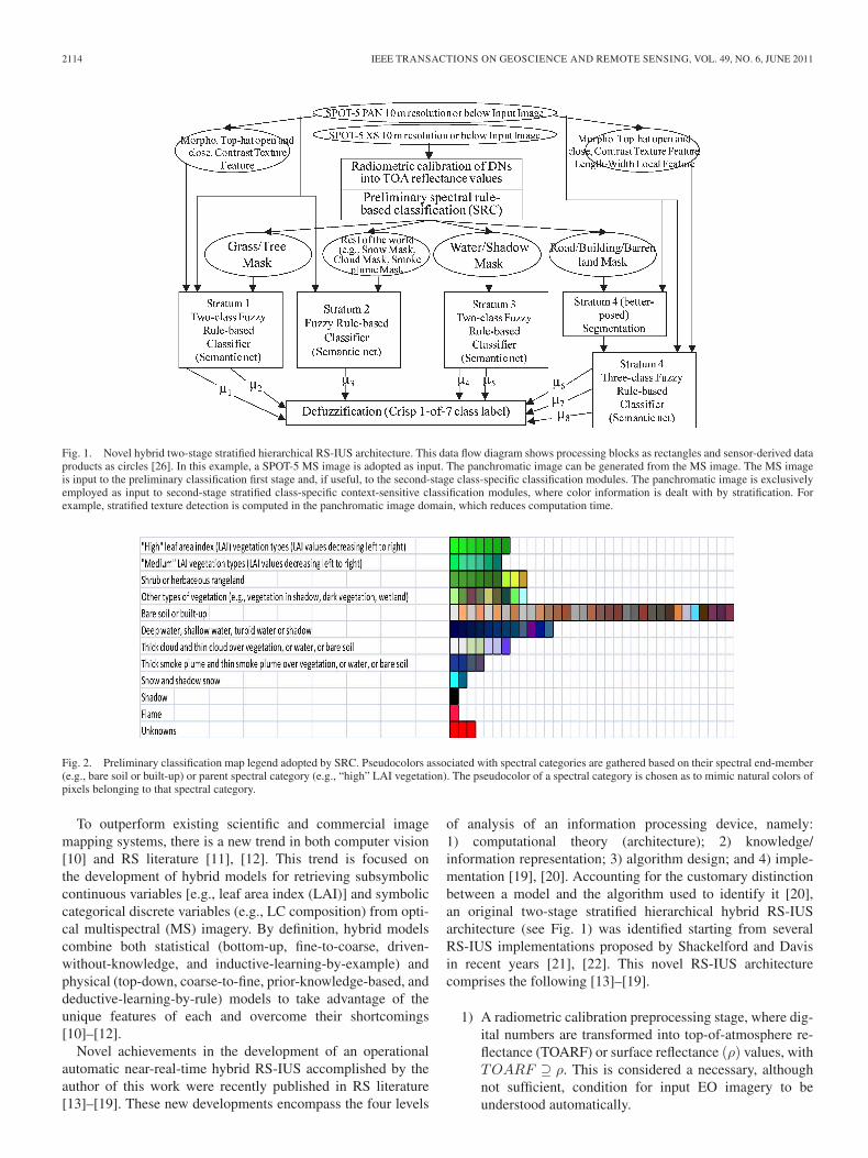
Fig. 2. Preliminary classification map legend adopted by SRC. Pseudocolors associated with spectral categories are gathered based on their spectral end-member(e.g., bare soil or built-up) or parent spectral category (e.g., “high” LAI vegetation). The pseudocolor of a spectral category is chosen as to mimic natural colors ofpixels belonging to that spectral category.

To outperform existing scientific and commercial imagemapping systems, there is a new trend in both computer vision[10] and RS literature [11], [12]. This trend is focused onthe development of hybrid models for retrieving subsymboliccontinuous variables [e.g., leaf area index (LAI)] and symboliccategorical discrete variables (e.g., LC composition) from opti-cal multispectral (MS) imagery. By definition, hybrid modelscombine both statistical (bottom-up, fine-to-coarse, driven-without-knowledge, and inductive-learning-by-example) andphysical (top-down, coarse-to-fine, prior-knowledge-based, anddeductive-learning-by-rule) models to take advantage of theunique features of each and overcome their shortcomings[10]–[12].

Novel achievements in the development of an operationalautomatic near-real-time hybrid RS-IUS accomplished by theauthor of this work were recently published in RS literature[13]–[19]. These new developments encompass the four levels

of analysis of an information processing device, namely:1) computational theory (architecture); 2) knowledge/information representation; 3) algorithm design; and 4) imple-mentation [19], [20]. Accounting for the customary distinctionbetween a model and the algorithm used to identify it [20],an original two-stage stratified hierarchical hybrid RS-IUSarchitecture (see Fig. 1) was identified starting from severalRS-IUS implementations proposed by Shackelford and Davisin recent years [21], [22]. This novel RS-IUS architecturecomprises the following [13]–[19].

1) A radiometric calibration preprocessing stage, where dig-ital numbers are transformed into top-of-atmosphere re-flectance (TOARF) or surface reflectance (ρ) values, withTOARF ⊇ ρ. This is considered a necessary, althoughnot sufficient, condition for input EO imagery to beunderstood automatically.

BARALDI: FUZZIFICATION OF SPECTRAL-RULE-BASED DECISION-TREE PRELIMINARY CLASSIFIER 2115

Fig. 3. (a) Four-band GMES-IMAGE2006 Coverage 1 mosaic, consisting of approximately 2000 four-band IRS-1C/-1D/-P6 LISS-III, SPOT-4 HRVIR, andSPOT-5 HRG images, mostly acquired during the year 2006, depicted in false colors: (Red) Band 4 (short-wave infrared), (green) Band 3 (NIR), and (blue) Band 1(visible green). Downscaled SR: 25 m. (b) Preliminary classification map automatically generated by SSRC from the mosaic shown in (a). Output spectralcategories are depicted in pseudocolors. Map legend is shown in Fig. 2. This result was achieved at the European Commission-Joint Research Center in October2008 and published in [13] and [16]. To the best of the author’s knowledge, this is the first example of such a high-level product automatically generated atcontinental scale at both the European Commission-Joint Research Center facility and elsewhere.

Fig. 4. (a) (Left) Web-enabled Landsat Data Project (http://landsat.usgs.gov/WELD.php). This is a joint NASA and USGS project providing seamless consistentmosaics of fused Landsat-7 ETM+ and MODIS data radiometrically calibrated into TOARF and surface reflectance. These mosaics are made freely availableto the user community. Each consists of 663 fixed location tiles. SR: 30 m. Area coverage: Continental U.S. and Alaska. Period coverage: Seven years. Producttime coverage: Weekly, monthly, seasonal, and annual composites. (b) (Right) Preliminary classification map automatically generated by LSRC from the 2008annual Web-enabled Landsat Data mosaic shown in (a). Output spectral categories are depicted in pseudocolors. Map legend is shown in Fig. 2. LSRC was run byL. Boschetti (University of Maryland) and Junchang Ju and D. Roy (University of South Dakota) in October 2010. To the best of the author’s knowledge, this isthe first example of such a high-level product automatically generated at continental scale at both the NASA and USGS.

2) A first-stage application-independent per-pixel (noncon-textual) top-down (prior-knowledge-based) preliminaryclassifier in the Marr sense [20].

3) A second-stage battery of stratified hierarchical context-sensitive application-dependent modules for class-specific feature extraction and classification.

The first-stage pixel-based preliminary classifier was de-signed and implemented as an original operational auto-matic near-real-time per-pixel multisource multiresolutionapplication-independent spectral-rule-based decision-tree clas-sifier (SRC). In [13]–[19], the coauthors worked independently

of the present author to provide an SRC with an independentscientific scrutiny for validation over a wide range of spatialconditions, time periods, optical imaging sensors, and geo-graphic extents ranging from local to regional and continentalscales, e.g., see Figs. 2–4.

To the best of the author’s knowledge, no unifying au-tomatic multisensor multiresolution RS image classificationcross-platform alternative to SRC can be found in existingliterature. For this reason, this work adopts SRC as a benchmark(reference) classifier and tries to answer the following question:How can the reference SRC first stage of a two-stage hybridRS-IUS be improved in operational contexts?


To answer this question, it is noteworthy that, for the sakeof simplicity, i.e., to reduce its number of free parameters,the original SRC decision-tree formulation adopts crisp (hard)membership functions (MFs) in combination with a hierarchi-cal modular structure to generate as output a sorted set of so-called spectral categories (equivalent to leaves of the decisiontree) [14], [15]. In terms of machine learning [23], the crispSRC decision tree belongs to the family of nonadaptive binarydecision trees. In general, nonadaptive decision trees are, first,prespecified, where intuition, domain expertise, and evidencefrom data are combined by a human expert in an ad hocprocess to come up with a final mapping of data [23, p. 391],and second, inherently sensitive to changes in hierarchy[23, p. 157].

The well-known conceptual foundation of fuzzy logic [24]appears as a valuable tool capable of improving the oper-ational quality indicators (QIs) (refer to Section II-C) of acrisp SRC decision tree. In particular, the replacement of acrisp SRC with a fuzzy SRC as the first stage of a two-stagestratified hierarchical hybrid RS-IUS is expected to achievethe following operational advantages based on theoreticalconsiderations.

1) Provide the first-stage preliminary classification outputmap (known as primal sketch in the Marr sense [20])with a superior information/knowledge representation[25], where component cover classes of mixed pixels(class mixture) are modeled (to be properly dealt with atthe second stage of the proposed two-stage hybrid RS-IUS architecture). In the words of Wang, “if knowledgerepresentation is poor, even sophisticated algorithms canproduce inferior outputs. On the contrary, improvementin representation might achieve twice the benefit with halfthe effort.”

2) Transform the crisp (hierarchical) SRC decision-treestructure into a fuzzy horizontal (flat) SRC system de-sign independent of hierarchy [23, pp. 157, 390]. Inoperational terms, a crisp-to-fuzzy SRC design trans-formation means that the fuzzy SRC software featuresenhanced maintainability/scalability/reusability (refer toSection II-C) [26], [27].

To counterbalance the expected advantages 1) and 2) afore-mentioned, it is noteworthy that a sequential (single-processsingle-thread) implementation of the inherently parallel fuzzySRC is expected to be computationally more intensive thana sequential implementation of the inherently sequential crispSRC decision tree (where every pixel-based MS data vectoractivates a single leaf of the decision tree). Fortunately, thecomputational overload of the fuzzy SRC versus the crisp SRCwould reduce to zero if parallel computation (single-processmultithread) is adopted instead.

Based on these theoretical considerations, the objective ofthis work is to replace the crisp pixel-based preliminary SRC(hierarchical) decision-tree first stage of a two-stage stratifiedhierarchical hybrid RS-IUS instantiation (see Fig. 1) with afuzzy (horizontal) SRC.

To better pose the fuzzy SRC system development projectand, at the same time, make it more ambitious, this work adopts

additional system requirements. In particular, the fuzzy SRCsystem is required not to lose any of the operational qualitiesof the crisp SRC decision tree. Since the crisp SRC performs“well” in operational contexts [13]–[19], then, in addition tomodeling class mixture, which is its added value, the fuzzy SRCis required to perform like the crisp SRC in terms of degree ofautomation, accuracy, robustness, and scalability.

These project requirements provide a set of necessary con-ditions for validation of the fuzzy SRC. They also mean that,in this work, no absolute accuracy measure of the fuzzy SRCis mandatory. Rather, a relative performance assessment of thefuzzy SRC in comparison with the crisp SRC, employed asa benchmark classifier, is necessary. The interested reader isreferred to existing literature for validation of the crisp SRCin the mapping of RS images acquired across time, space, andsensors [13]–[19].

The rest of this paper is organized as follows. In Section II,basic concepts and definitions employed in this work are madeexplicit. SRC-specific concepts and SRC-related works arereviewed in Section III. In Section IV, the fuzzy SRC systemimplementation strategy is sketched. An experimental sessionis selected in Section V. Experimental results are discussed inSection VI. Conclusions are reported in Section VII.

II. BASIC CONCEPTS AND DEFINITIONS

In Section I, the goal of this work is defined as the trans-formation of an operational automatic nonadaptive (predefined)crisp binary SRC (hierarchical) decision tree into a nonadaptivefuzzy (horizontal) SRC capable of losing none of the opera-tional qualities of the former.

In general, basic concepts and definitions adopted in thiswork are not community-agreed and/or tend to be ignored inRS common practice. In this section, they are made explicit toreduce their potential degree of ambiguity and thus contributeto making this paper self-contained.

A. S- and Z-MFs

In the traditional field of artificial intelligence [23], systemsof fuzzy IF–THEN rules consist of a set of simultaneousunivariate premises (conditions on scalar input variables) andan output consequence (action), e.g., IF (temperature is low)AND (pressure is high) THEN (ignition value is 0.7). Linguisticterms specifying input and output values are fuzzy sets (FSs)with MFs. FSs in the antecedent (IF) part are called input FSs,and FSs in the consequent (THEN) part of fuzzy rules arecalled output FSs. By definition [14], an FSL is an orderedpair FSL(xn) = {(xn, μL(xn))|μL(xn) ∈ [0, 1], xn ∈ �, n ∈{1, N}}, where N is the sample set size and μL(xn) is anMF associated with a linguistic label L (e.g., low, medium, andhigh). An MF maps the scalar input space of real numbers � tothe bounded nonnegative real membership space [0, 1]. In thiscase, the IF–THEN rule is termed fuzzy. In practice, an FSL isa class-specific and linguistic label L-specific set of value pairs,(xn, μL(xn)), possessing a continuum of membership grades,i.e., there is no sharp boundary among xn elements that belongto this class and those that do not [24]. If the membership space


consists of only two discrete values, equivalent to zero and one,then the IF–THEN rule is not termed fuzzy but is hard or crisp.

Typical examples of fuzzy MFs are the 1-D Gaussian MFsand the S- and Z-MFs. A typical implementation of a fuzzyS-function is the following [28]:

μL,S(xn)

= S (xn; a, b, c : a < (b = (a+ c)/2) < c)

=

⎧⎪⎨⎪⎩

0, xn≤a2 {(xn − a)/(c− a)}2 , a<xn≤b, c>a1− 2 {(xn − c)/(c− a)}2 , b<xn≤c, c>a1, xn>c.

(1)

This S-function is controlled by the two free parameters a and c.The derived variable b = (a+ c)/2 denotes the crossover point,where μL,S(b) = 0.5. The bandwidth parameter Δb of theS-function is defined as 0 < Δb = b− a = c− b. The Z-function is derived from the S-function as follows:

μL,Z(xn) =Z(xn; a, b, c)

= 1− S (xn; a, b, c : a<b=(a+ c)/2<c) . (2)

In the crisp instantiation of the S- and Z-functions, param-eters a and c of (1) and (2) tend to coincide, i.e., a → b =[(a+ c)/2] = Th → c, then Δb → 0. In this case, the crispversion of (1) becomes μL,S(xn) = S(xn;Th) = {(0 if xn ≤Th) OR (1 if xn > Th)}.

B. Absolute Radiometric Calibration Into TOARF Values

As reported in Section I, SRC requires as input an MS imageradiometrically calibrated into TOARF or surface reflectance(ρ) values, the latter being an ideal (atmospheric noise-free)case of the former, i.e., TOARF ⊇ ρ [13]–[19]. This allowsSRC to consider the inherently ill-posed atmospheric correc-tion preprocessing of an input MS image optional rather thancompulsory. It also means that SRC must employ as input MSimagery provided with radiometric calibration metadata files.

Table I reports on the relationship existing between com-mercial RS-IUSs and the radiometric calibration constraintconsidered mandatory by the international Quality AssuranceFramework for EO (QA4EO) [38] delivered by the WorkingGroup on Calibration and Validation of the Committee of EarthObservations (CEOS), the space arm of GEO [3]. Table Ishows that, first, no existing commercial RS-IUS software,except for the ERDAS ATCOR3 software module [7], requiresradiometric calibration preprocessing. In recent papers, thepresent author highlighted the fact that by making RS data wellbehaved and well understood, radiometric calibration not onlyensures the harmonization and interoperability of multisourceobservational data according to the QA4EO guidelines [38]but is also a necessary, although insufficient, condition forautomating the quantitative analysis of EO data [13]–[19]. Thisnecessary condition for automatic EO data interpretation agreeswith common sense, summarized by the expression “garbagein, garbage out.” In the terminology of machine learning and

TABLE IEXISTING COMMERCIAL RS-IUSs AND THEIR DEGREE OF MATCH WITH

THE INTERNATIONAL QA4EO GUIDELINES

computer vision, the radiometric calibration constraint aug-ments the degree of prior knowledge of an RS-IUS requiredto complement the intrinsic insufficiency (ill-posedness) of(2-D) image features, i.e., radiometric calibration makes theinherently ill-posed computer vision problem better posed.

To summarize, in disagreement with the QA4EO guidelines,most existing scientific and commercial RS-IUSs, such as thoselisted in Table I, do not require RS images to be radiometricallycalibrated and validated. As a consequence, according to theaforementioned necessary condition for automating the quan-titative analysis of EO data, these RS-IUSs are semiautomaticand/or site specific (since one scene may represent, for example,apples, while any other scene, even if contiguous or overlap-ping, may represent, for example, oranges) (refer to Table I).Second, Table I shows that, unlike SRC, the ERDAS ATCOR3requires as input an MS image radiometrically calibrated intosurface reflectance ρ values exclusively. This implies that theERDAS ATCOR3 software considers mandatory the inher-ently ill-posed and difficult-to-solve MS image atmosphericcorrection preprocessing stage which requires user interventionto make it better posed [7]. Thus, unlike SRC, the ERDASATCOR3 satisfies the necessary condition for automating thequantitative analysis of EO data, but is insufficient to provide anRS image classification problem with an automatic workflowrequiring no empirical parameter to be user defined based onheuristic criteria.


C. Operational QIs of an RS-IUS

In operational contexts, an RS-IUS is defined as a lowperformer if at least one among several operational QIs1 scoreslow. Typical operational qualities of an RS-IUS encompass thefollowing [26], [27].

1) Degree of automation. For example, a data processingsystem is automatic when it requires no user-definedparameter to run; therefore, its user-friendliness cannotbe surpassed. When a data processing system requiresneither user-defined parameters nor reference data sam-ples to run, then it is termed “fully automatic” [35].Section II-B reports that radiometric calibration is a nec-essary, although insufficient, condition for automating thequantitative analysis of EO data [13]–[19].

2) Effectiveness, e.g., classification accuracy.3) Efficiency, e.g., computation time, memory

occupation, etc.4) Economy (costs). For example, open-source solutions are

welcome to reduce costs of software licenses.5) Robustness to changes in the input data set, e.g., changes

due to noise in the data.6) Robustness to changes in input parameters, if any.7) Maintainability/scalability/reusability to keep up with

changes in users’ needs and sensor properties.8) Timeliness, defined as the time span between data acqui-

sition and product delivery to the end user. It increasesmonotonically with manpower, e.g., the manpower re-quired to collect site-specific training samples.

The aforementioned list of operational QIs is neither irrel-evant nor obvious. For example, a low score in operationalQIs may explain why the literally hundreds of so-called novellow-level (subsymbolic) and high-level (symbolic) image pro-cessing algorithms presented each year in scientific literaturetypically have a negligible impact on commercial RS imageprocessing software [5]. This conjecture is consistent with thefact that most works published in RS literature assess andcompare spaceborne image classification algorithms in termsof mapping accuracy exclusively, which corresponds to thesole operational performance indicator 2) listed earlier. More-over, these classification accuracy estimates are rarely providedwith a degree of uncertainty in measurement [as a negativeexample not to be imitated (see [36])]. This violates well-known laws of sample statistics [29], [30], [37], together with

1Any evaluation measure is inherently noninjective [17]. For example, inclassification-map accuracy assessment and comparison, different classificationmaps may produce the same confusion matrix while different confusion matri-ces may generate the same confusion matrix accuracy measure, such as theoverall accuracy (OA). These observations suggest that no single universallyacceptable measure of quality, but instead a variety of quality indices, shouldbe employed in practice [29], [30]. To date, this general conclusion is neitherobvious nor community-agreed. For example, in computer vision and RS, thisconclusion implies that when a test image and a reference (original) imagepair is given, common attempts to identify a unique (universal) reliable imagequality index, such as the relative dimensionless global error ERGAS proposedin [31], the universal image quality index Q [32], the global image qualitymeasure Q4 [33], and the quality index with no reference QNR [34], areinherently undermined as contradictions in terms.

common sense envisaged under the international guidelines ofthe QA4EO. In particular, the QA4EO guidelines require thatevery sensor-derived data product, generated across a satellite-based measurement system’s processing chain, be providedwith metrological/statistically based QIs featuring a degree ofuncertainty in measurement [38].

To summarize, the operational quality assessment of manyRS-IUSs presented in literature does not satisfy the interna-tional QA4EO recommendations. In practice, operational qual-ities of published RS-IUSs remain largely unknown. Based onthe evidence that these RS-IUSs have had a negligible impacton commercial and scientific RS image processing softwaretoolboxes, the conclusion is that these RS-IUSs are expectedto score poorly in operational contexts.

D. Crisp Classification Accuracy Measures andConfidence Interval

Section II-C mentions that, in violation of common sense andsample statistics envisaged under the GEO-CEOS internationalQA4EO guidelines, most works published in RS literatureassess and compare alternative spaceborne image classificationalgorithms exclusively in terms of mapping accuracy providedwith no confidence interval.

According to sample statistics, it is well known that anyclassification OA probability estimate pOA ∈ [0, 1] is a randomvariable (sample statistic) with a confidence interval (errortolerance) ±δ associated with it, where 0 < δ < pOA ≤ 1 [29],[30], [37]. In other words, pOA ± δ is a function of the specifictest data set used for its estimation and vice versa [37]. Forexample, given a target classification accuracy probability pOA

and a test sample set size Mtest comprising independent andidentically distributed reference samples (in RS common prac-tice, this hypothesis is often violated due to spatial autocorrela-tion between neighboring pixels selected as reference samples),the half width δ of the error tolerance ±δ at a desired confidencelevel (e.g., if confidence level = 95%, then the critical value is1.96) can be computed as follows [29], [37], [39]:

δ =

√(1.96)2 · pOA · (1− pOA)

Mtest. (3)

For each cth class simultaneously involved in the classificationprocess, with c = 1, . . . , C, where C is the total number ofclasses, it is possible to prove that (refer to [42, p. 294])

δc =

√χ2(1,1−α/C) · pOA,c · (1− pOA,c)

mtest,c, c = 1, . . . , C

(4)

where α is the desired level of significance, i.e., the risk that theactual error is larger than δc (e.g., α = 0.07), (1− α/C) is thelevel of confidence, and χ2

(1,1−α/C) is the upper (1− α/C) ∗100th percentile of the chi-square distribution with 1 DOF. Forexample, if α = 0.04 and C = 4, then the level of confidence is(1− 0.04/4) = 0.99, and then, χ2

(1,0.99) = 6.63.


Starting from (4), the class-specific training data set cardi-nality, mtest,c, with c = 1, . . . , C, required for target δc, pOA,c,and α parameters becomes

mtest,c =χ2(1,1−α/C) · pOA,c · (1− pOA,c)

δ2c,

c = 1, . . . , C. (5)

Typical values of classification accuracy and confidence in-terval are employed as a benchmark by the RS community.The target OA pOA ∈ [0, 1]± δ = (3) is fixed at 0.85 ± 2%,in agreement with the U.S. Geological Survey (USGS) classifi-cation system constraints [40]. The class-specific classificationaccuracies pOA,c ∈ [0, 1]± δc = (4), c = 1, . . . , C, should beabout equal to, and never below, 70% [31], whereas a reason-able reference standard for δc is about 5%.

In this paper (see Section V-D), the test data set consists ofreference samples belonging to four target spectral categories(equivalent to LC class sets; refer to Section III below and [15]),namely, “either woody vegetation or cropland or grassland,”“rangeland,” “either bare soil or built-up,” and “water”;thus, C = 4 (refer to Section V-D). Since C = 4, if α = 0.04,then (1− α/C) = 0.99, and χ2

(1,0.99) = 6.63 (refer to previousdiscussion). If δc is set equal to 5% and the target pOA,c = 85%,then the required cardinality of class-specific reference samplesbecomes mtest,c = (5) ≈ 340, c = 1, . . . , 4.

E. Fuzzy Classification Accuracy Measures

One additional advantage of using “soft” classifiers, as op-posed to “hard” ones, is that the former provide the possibilityof using many measures for accuracy assessment of a classifi-cation beyond the standard pOA ∈ [0, 1] and confusion matrix[29], [39]. A number of approaches are available, e.g., fuzzyoperators [41], fuzzy distances and the Shannon entropy [42],the index of fuzziness [43], the fuzzy OA (FOA) [44], severalmeasures of fuzzy similarity [45], and the fuzzy error matrix,which is a generalization of the standard confusion matrix andprovides several indicators of classification accuracy such asthe FOA and, for each category, the producer’s accuracy andthe user’s accuracy [44].

In this paper, the fuzzy output of the proposed fuzzy SRC isnot evaluated by any of the fuzzy accuracy measures mentionedabove before “hardening” occurs. The reason is that no pixel-based ground-truth contribution of each category in the selectedset of test images was available (see Section V-D). As a matterof fact, class mixture information would be very tedious, expen-sive, and difficult to acquire based on field sites, existing maps,and tabular data; indeed, class mixture ground truth is almostnever available in practice.

Considering that this paper is focused on a relative as-sessment of the fuzzy SRC in comparison to the crisp SRCrather than on an absolute validation of the former (referto Section I), the absence of a reference data set providingground-truth contributions to mixed pixels can be overcome bythe comparison of the reference crisp SRC output map withthe “hardened” (defuzzified) version of the fuzzy SRC outputmap, where “multiple winners” (see Section IV-F) are resolved(defuzzified), i.e., they are assigned to one of the best matchingspectral categories.

III. SRC-SPECIFIC CONCEPTS AND SRC-RELATED

WORKS IN RS IMAGE CLASSIFICATION

As stated in Section I, this work aims at improving theoperational QIs of the first automatic multisensor multireso-lution hybrid RS-IUS proposed in [13]–[19]. A well-knownbook on the development of hybrid RS-IUS is, for example,[11]. In RS journals, aside from classic publications such as[25], [46], and [47], few recent papers deal with the machinelearning algorithms of potential interest to this work, such asthe following.

1) Adaptive decision trees, such as the well-known clas-sification and regression binary decision-tree algorithmCART, taken from machine learning [23].

2) Nonadaptive decision trees, like SRC [13]–[19].3) Adaptive fuzzy-rule-based systems [48], which require a

reference data set which is typically scene specific, ex-pensive, tedious, and difficult or impossible to collect [1].

4) Nonadaptive fuzzy-rule-based systems [21], [22], [49],[50], whose tuning is accomplished by a human expertrelying on his/her intuition, domain expertise, and evi-dence from data observation [23]. For example, in [50],FSs employed in fuzzy rules model the size and contrastof image structures investigated via the multiscale differ-ential morphological profile [51].

5) Semantic nets, either directed or nonoriented, eithercyclic or acyclic, consisting of nodes (representing con-cepts, i.e., classes of objects in the world) linked byedges (representing relations, e.g., PART-OF, A-KIND-OF, spatial relations, temporal transitions, etc.) betweennodes [11], [52]–[54].

Semantic nets deal with the attentive vision phase [55]–[58]; as a consequence, they cope with the artificial and in-trinsic insufficiency of (2-D) image informational primitivesextracted by preattentional vision2 [11], [15]–[17]. In otherwords, in semantic nets, there is no attempt to reduce the part ofill-posedness of the computer vision problem due to the artifi-cial insufficiency of image primitives (rather, this reduction is

2The main role of a biological or artificial visual system is to backprojectthe information in the (2-D) image domain to that in the (3-D) scene domain[11]. In greater detail, the goal of a visual system is to provide plausible(multiple) symbolic description(s) of the scene depicted in an image by findingassociations between subsymbolic (2-D) image features with symbolic (3-D)objects (concepts) in the scene (e.g., a building, a road, etc.). Subsymbolic (2-D)image features are either points or regions or, vice versa, region boundaries, i.e.,edges, provided with no semantic meaning. In literature, (2-D) image regionsare also called segments, (2-D) objects, patches, parcels, or blobs.

There is a well-known information gap between symbolic information inthe (3-D) scene and subsymbolic information in the (2-D) image (e.g., dueto dimensionality reduction and occlusion phenomena). This is called theintrinsic insufficiency of image features. It means that the problem of imageunderstanding is inherently ill-posed and, consequently, very difficult to solve[11], [15].

In functional terms, biological vision combines preattentive (low-level)visual perception with an attentive (high-level) vision mechanism [55]–[57].

1) Preattentive (low-level) vision extracts picture primitives based ongeneral-purpose image processing criteria independent of the scene underanalysis. It acts in parallel on the entire image as a rapid (< 50 ms) scanningsystem to detect variations in simple visual properties. It is known that thehuman visual system employs at least four spatial scales of analysis [58].

2) Attentive (high-level) vision operates as a careful scanning systememploying a focus of attention mechanism. Scene subsets, corresponding toa narrow aperture of attention, are looked at in sequence and each step isexamined quickly (20–80 ms).


exactly the objective of the SRC first stage in a two-stage hybridRS-IUS [15]–[17]). To date, semantic nets lack flexibility andscalability, i.e., they are unsuitable for commercial RS imageprocessing software toolboxes and remain limited to scientificapplications.

About SRC, it is noteworthy that, although it belongs tothe class of nonadaptive decision trees (see earlier discussion),it was not conceived as a stand-alone classifier; rather, SRCis to be employed as the first stage of a two-stage stratifiedhierarchical hybrid RS-IUS. As stated in Section I, the degreeof novelty of a two-stage stratified hierarchical hybrid RS-IUS provided with a first-stage operational automatic SRCdecision tree [13]–[19] (see Fig. 1) encompasses the four levelsof analysis of an RS-IUS [19], [20]. Original SRC-specificconcepts, definitions, and properties to be recalled in the designSection IV and experiment Section V are summarized hereafter.

The core definition introduced by SRC is that of spectral-based semiconcept or spectral category or LC class set orspectral end member [15]. A spectral category is equivalent to asemantic conjecture based exclusively on spectral (i.e., chro-matic and achromatic) properties. Spectral properties are inher-ently noncontextual, i.e., pixel based. For example, one pixel isred like a brick no matter what the colors of its neighboring pix-els are. From a spaceborne MS image employed as input, SRCautomatically generates as output a preliminary map or primalsketch in the Marr sense (refer to Section I) [20]. A preliminarySRC map consists of six spectral supercategories (spectral endmembers), namely: 1) “clouds” (CL); 2) “either snow or ice”(SN); 3) “either water or shadow” (WASH); 4) “vegetation”(V), equivalent to “either woody vegetation or cropland orgrassland or (shrub and brush) rangeland”; 5) “either bare soilor built-up” (BB); and 6) “outliers.”3 Spectral supercategoriesare mutually exclusive and totally exhaustive, in line with theCongalton definition of a classification scheme [29]. Spectralsupercategories can split into several subcategories [14]. In thewords of Di Gregorio and Jansen [60], although it generates alarge number of spectral subcategories, SRC consists of a smallnumber of classification modules of spectral supercategories.

SRC is an operational automatic system of systems, in linewith the visionary goal of a GEOSS [3]. It comprises a masterseven-band Landsat-like SRC (LSRC) [14] plus five down-scaled LSRC subsystems whose spectral resolution overlapswith, but is inferior to, Landsat’s [15]. These downscaledLSRC subsystems are identified as follows: 1) the four-bandSPOT-like SRC (SSRC); 2) the four-band Advanced VeryHigh Resolution Radiometer (AVHRR)-like SRC (AVSRC);3) the five-band ENVISAT Advanced Along-Track ScanningRadiometer-like SRC (AASRC); 4) the four-band IKONOS-like SRC (ISRC); and 5) the three-band Disaster MonitoringConstellation-like SRC (DSRC). As input, SRC requires aradiometrically calibrated MS image acquired by almost any ofthe ongoing or future planned satellite optical missions (refer toTable II).

3The adopted LC nomenclature is based on the USGS classification hierarchy[59], the Coordination of Information on the Environment, the Food andAgriculture Organization of the United Nations (FAO) Land Cover Classifica-tion System [60], and the International Geosphere–Biosphere Programme LCunits [49].

For a complete discussion of these subjects, the interestedreader is referred to [13]–[19].

IV. PROPOSED CRISP-TO-FUZZY SRCSYSTEM ADAPTATION

Starting from the problem and opportunity recognition pro-posed in Section I, namely, the fuzzification of the original SRCsystem of systems presented in [14] and [15], the goal of thispaper can be reformulated in mathematical terms.

A. Fuzzy SRC MF

The original SRC, employed as a reference (see Section I),adopts crisp S- and Z-functions parameterized by a crispthreshold Th ∈ �+

0 found in [14, Tab. III] (see Section II-A).These crisp MFs should be replaced by fuzzy S- and Z-MFs,namely, (4) and (5), respectively, controlled by the parameterpair a < c, such that a = f1(Th) < b = [(a+ c)/2] = Th ∈�+

0 < c = f2(Th), with f1(·) = f2(·), where b = Th is thecrossover point such that μL,S(Th) = 0.5, with bandwidth 0 <Δb = b− a = c− b (see Section II-A). Obviously, if the fuzzyS- and Z-function bandwidth Δb → 0, i.e., if a → b = Th → c,then the fuzzy and the crisp SRC are expected to perform in thesame way. This simple observation provides a useful criterionin validating the fuzzy SRC implementation against theory.

B. Fuzzy SRC Data Coding

The bounded nonnegative real membership space [0, 1] isbyte coded, i.e., it is discretized into range {0, 255} to reducedynamic/hard-disk memory occupation of membership valueswhose discretization error is 1/255 = 0.4%.

C. Fuzzy SRC Operators

In [14, Tab. VII], where a hierarchy of logical expressionsgenerates a set of Boolean spectral categories, the Boolean-AND operator is replaced by the fuzzy-AND (minimum), theBoolean-OR operator is replaced by the fuzzy-OR (maximum),and the unary Boolean-NOT(x) operator of the Boolean vari-able x ∈ {0, 1} is replaced by operator (255-X), with byte-coded membership value X ∈ {0, 255}. For more details aboutinformation combination operators, refer to [66].

D. Fuzzy SRC Software Architecture

1) In line with the Congalton definition of a classificationscheme [29], the crisp SRC decision tree provides a mutu-ally exclusive and totally exhaustive mapping of the inputimage into a discrete and finite set of spectral categoriesincluding class “unknown” (outliers) [14], [40] (refer toSection III). In the original (L)SRC decision tree pro-posed in [14], mutual exclusiveness of spectral categoriesis guaranteed by a combination of (crisp) MFs with theirorder of presentation. The prior knowledge of this orderof presentation is embedded in the hierarchical structureof a decision tree [23], [61]. This modular hierarchy


TABLE IISRC SYSTEM OF SYSTEMS: LIST OF SPACEBORNE OPTICAL IMAGING SENSORS ELIGIBLE FOR USE

of crisp MFs is flattened in a fuzzy-rule-based systemindependent of hierarchy [23], called fuzzy SRC, wherefirst, fuzzy MFs are computed in parallel (horizontally,with the same level of priority) and, second, membership

values are defuzzified (refer to Section I and the followingdiscussion).

2) In the crisp SRC implementation, input data vectors thatfall outside the (hyperdimensional) domain of activation


of every spectral category are assigned to class “un-known” [14]. In the fuzzy SRC instantiation, outliers aredetected when the membership value of the winning spec-tral category falls below a system threshold parameter tobe user defined based on heuristics. Since this thresholdidentifies the minimum normalized membership valueconsidered acceptable by the user, this threshold parame-ter features an intuitive physical meaning. Therefore, it iseasy to select (by default, it is set equal to 0.2, i.e., pixelswhose maximum membership is below 0.2 are assignedto class “unknown”).

3) A defuzzification stage is built (e.g., in Fig. 1, a de-fuzzification stage is visible at the output of the secondstage of the two-stage hybrid RS-IUS). For every pixel,the winning spectral category is the one featuring thehighest membership value (i.e., defuzzification adoptsa fuzzy OR operator). If multiple winners exist for agiven pixel, then an empirical strategy can be chosen toselect one winning category among eligible cowinners(see following discussions).

E. Fuzzy SRC-Specific Output Products

To deal with mixed pixels featuring a class mixture, threeoriginal output products are generated by the fuzzy SRC inaddition to those generated by the crisp SRC.

1) The first fuzzy SRC-specific output product is a con-tinuous maximum membership (MMB) value image inrange [0, 1] discretized into byte-coded values {0, 255}.The fuzzy membership value of pixels belonging to class“outliers” (unknown) is conventionally set to zero in theMMB output image.

2) The second fuzzy SRC-specific output product is an inte-ger image, called multiple winner counter (MWC), withMWC ≥ 1. It provides the number of winners pertainingto any pixel such that, at the end of the classificationprocess, MWC ≥ 1 is image-wide; in fact, since SRCprovides a totally exhaustive mapping of the input image(see Section III), then each pixel is mapped onto at leastone spectral category, including class “unknown.” Pixelsfeaturing multiple winners, such that (MWC > 1), canbe mapped onto a special binary mask to be consideredwith special attention. For example, each pixel featuring(MWC > 1) can be defuzzified, i.e., assigned to onespectral category selected from its list of multiple win-ners, based on arbitrary user-defined application-specificcriteria. Since symbolic spectral categories [e.g., “vege-tation,” “clouds,” etc., (refer to Section III)] are easy tounderstand by both RS experts and nonexpert users whoare naturally familiar with symbolic reasoning, empiricaldefuzzification criteria for pixels featuring (MWC >1) are easy (intuitive) to define. For example, a mixedpixel belonging to a (3-D) LC class wetland, featuresmultiple winners at primal sketch, for example, spectralcategories “vegetation” and “either water or shadow”;between these two winning spectral categories, that pixelis arbitrarily assigned to the former by the defuzzificationstrategy.

3) The third fuzzy SRC-specific output product is a bi-nary map called mixed pixel mask (MPM) ∈ {0, 1} ={False,True}, where False = 0 and True = 1. It iden-tifies pixels for which the difference between the bestmembership and the second best membership is smallerthan a given threshold α ∈ [0, 1] (by default, α = 0.2).These are pixels whose second best membership valueis considered “close enough” to the winning (largest)membership value to be considered mixed pixels. Thesemixed pixels include pixels affected by multiple winners,i.e., (MPM EQ True) ⊇ (MWC > 1) ∀ α ≥ 0. If α =0, then relationship (MPM EQ True) == (MWC > 1)must hold. These two relationships provide a useful de-bugging tool in verifying the adequacy of the fuzzy SRCimplementation against theory (refer to Section V-C1).

F. Adopted Terminology

For the sake of simplicity, the following terminology isadopted. Pixels belonging to the binary mask (MWC > 1) arecalled multiple winners. Pixels belonging to the binary mask(MPM EQ True) are identified as “mixed pixels,” such that(MPM EQ True) ⊇ (MWC > 1).

To summarize, at the second stage of a two-stage strati-fied hierarchical hybrid RS-IUS whose pixel-based preliminaryclassification first stage is the fuzzy SRC (see Fig. 1), multiplewinners, for which condition (MWC > 1) holds, should behandled with special attention. They represent the worst casewithin the set of mixed pixels (MPM EQ True) ⊇ (MWC >1) ∀ α ≥ 0.

V. EXPERIMENTAL SESSION DESIGN

To provide a quantitative validation of the novel fuzzy SRC,the Prechelt test session criteria [62] are integrated with exper-imental constraints found in [17] and [63]. These experimentalsession design criteria are summarized next.

1) To test the robustness of a novel approach to changes inthe input data set, select at least two real and/or standard/appropriate data sets. For example, a typical standard/appropriate data set is a synthetic data set of standardquality whose signal-to-noise ratio is known and con-trolled by the user.

2) Based on [63], a set of RS images suitable for comparingthe performance of alternative algorithms should have thefollowing characteristics: 1) consistent with the aim oftesting; 2) as realistic as possible, i.e., each member ofthe set should reflect a given type of images encounteredin practice; and 3) mutually uncorrelated, to reduce thecardinality of the test data set.

3) Employ a battery of measures of success [QIs (refer toSection II-C)] capable of dealing with the well-knownnoninjective property of any quality index (refer to foot-note 1) [17].

4) For comparison purposes, select at least one alternativeexisting well-known approach as a benchmark, e.g., inour case, the crisp SRC is employed as a reference (seeSection I).


The aforementioned experimental session quality criteria aresatisfied as described next.

A. Selection of Competing Classifiers

The four fuzzy LSRC, SSRC, AVSRC, and ISRC subsys-tems of the integrated fuzzy SRC system of systems (referto Section III) are quantitatively compared against their crispcounterparts employed as a reference (refer to Section I). Inthis comparison, the SRC subsystems AASRC and DSRC areomitted to reduce the paper length without losing any meaning-ful information. AASRC and DSRC differ from AVSRC andISRC, respectively, by a single band in the visible portion of theelectromagnetic spectrum (see Table II). However, SRC assignsslight importance (low weight) to evidence collected fromvisible bands in its multiple-criteria decision-making process(so as not to be very sensitive to haze and atmospheric effects[14]–[17]). This means that output maps of AASRC and DSRCare very similar to (i.e., highly correlated with) those of AVSRCand ISRC, respectively (typically, these map pair correlationvalues are greater than 0.9 when synthetic images are employedas input).

B. Selection of the Test Image Set

Three real-world Landsat images are selected to depict avariety of natural and anthropogenic landscapes at differentgeographic footprints and acquisition times. Next, the selectedLandsat images are radiometrically calibrated into TOARFvalues [13]–[19]. Finally, to make result assessment and com-parison easier for a domain expert, one test subimage is selectedfrom each radiometrically calibrated seven-band Landsat im-age. The three test subimages are as follows: 1) a Landsat-7Enhanced TM Plus (ETM+) subimage of the city area ofBologna, Italy, 434 (lines) × 400 (columns) pixels in size, path:192, row: 029, acquisition date: June 20, 2000 [see Fig. 5(a)];2) a Landsat-7 ETM+ subimage of a seaside area in Sicily, Italy,400 × 400 pixels in size, path: 188, row: 034, acquisition date:September 26, 1999 (see Fig. 9); and 3) a Landsat-7 ETM+subimage of a mountainous snow-covered area in NorthernItaly, 400 × 400 pixels in size, path: 193, row: 028, acquisitiondate: September 13, 1999 (see Fig. 10).

These three radiometrically calibrated seven-band Landsat-7ETM+ subimages are suitable for comparing the novel fuzzyLSRC against the original crisp LSRC proposed in [14] (referto Section III).

To test the fuzzy SSRC, AVSRC, and ISRC subsystemsagainst their crisp counterparts (refer to Section V-A) [15],synthetic sensor-specific radiometrically calibrated MS imagesare generated from the three test seven-band Landsat subimagesshown in Figs. 5(a), 9, and 10. The synthetic subimages aregenerated as follows.

1) SSRC requires as input a four-band (G, R, near-IR (NIR),MIR1) SPOT-like imagery. Thus, the Landsat bands B,MIR2, and TIR are removed from the three test Landsatsubimages (see Table II).

2) AVSRC requires as input a four-band (R, NIR, MIR1,TIR) AVHRR-like imagery. Thus, the Landsat bands B,

G, and MIR2 are removed from the three test Landsatsubimages (see Table II).

3) ISRC requires as input a four-band (B, G, R, NIR)IKONOS-like imagery. Thus, the Landsat bands MIR1,MIR2, and TIR are removed from the three test Landsatsubimages (see Table II).

The proposed MS image selection/generation strategy allowssensitivity analysis of the fuzzy LSRC, SSRC, AVSRC, andISRC systems [16], [19]. Differences in performance amongthese classifiers are exclusively due to differences in spectralresolution of the given set of test images (sharing the samegeographic footprint, time of acquisition, sensor calibration,and SR).

It is noteworthy that, according to some reviewers, “thegeneration of these “synthetic” images appears to be critical.Synthetic bands are selected on the basis of their wavelengthrange exclusively, while optical sensor parameters such as SR,spectral response functions, swath width, incident angle, etc.,are ignored. Thus, the use of synthetic images seems interestingin regard to missing spectral information, but not in regard tothe transferability of the approach to other sensor sources.” Thisskepticism is reasonable, but not justified. It is obvious to saythat synthetic and real-world images are complementary and byno means alternative for testing [62], [63]. For example, say thatSRC is capable of detecting spectral signatures typical of redapples, yellow bananas, and orange oranges. At a given SR, leta picture of apples and bananas be taken. If a pixel is a mixtureof red apples and yellow bananas, then that pixel looks orange.Since SRC is assumed to be provided with an orange objectmodel, it labels that mixed pixel as orange like an orange. Thispixel mapping (for example, that pixel looks like an orange) isstrictly correct, although SRC fails to provide any informationabout pixel unmixing. If the same picture of apples and bananasis taken at a finer SR capable of reducing the presence ofmixed pixels to null, then the SRC orange detector would neverfire and all image pixels would be labeled by SRC as eitherred (like an apple) or yellow (like a banana). To conclude, ifthe spatial/spectral resolution of an MS image varies, then thebehavior of the SRC must vary, but remain consistent with thevarying image information content.

C. Fuzzy SRC System Consistency Checks and ModelSelection Criteria

1) Consistency Checks: The following consistency checksare scheduled to verify the adequacy of the fuzzy SRCversion against both theory and the reference crisp SRCimplementation.

1) Relationship (MPM EQ True) ⊇ (MWC > 1) holds∀ α ≥ 0. As a special case, if α = 0, then equality(MPM EQ True) == (MWC > 1) must hold (refer toSection IV-E).

2) If the fuzzy S- and Z-function bandwidth parameter 0 <Δb = b− a = c− b tends to zero, i.e., if Δb → 0, thena → b = Th → c. In practice, if Δb → 0, then the fuzzySRC adopts crisp S- and Z-functions (see Section II-A).If Δb → 0, the fuzzy SRC consistency checks can betwofold.


Fig. 5. (a) Zoomed image of the city of Bologna, Italy, extracted from a Landsat 7 ETM+ image (path: 192, row: 029, acquisition date: June 20, 2000),radiometrically calibrated into TOARF values and depicted in false colors (R: band TM5 = MIR1, G: band TM4 = NIR, B: band TM1 = B). (b) Preliminaryclassification map, depicted in pseudocolors, automatically generated by the crisp LSRC from the radiometrically calibrated image shown in (a). Map legendis shown in Fig. 2. The association of symbolic spectral categories with pseudocolors found in nature allows an intuitive (qualitative, visual) assessment of thepreliminary classification map accuracy in comparison with the input image depicted in false colors, as shown in (a). (c) Preliminary classification map, depictedin pseudocolors, generated by the fuzzy LSRC from the radiometrically calibrated image shown in (a), with bandwidth Δb = 0. Map legend is shown in Fig. 2.Multiple winners, i.e., pixels featuring (MWC > 1), are depicted in black. They are due to the fact that the hierarchical structure of the crisp (L)SRC has beenreplaced by a flat modular organization of the fuzzy SRC. In line with theory, the fuzzy LSRC with Δb = 0 looks the same as (b) aside from the multiple winnersdepicted in black. (d) Preliminary classification map, depicted in pseudocolors, generated by the fuzzy LSRC from the radiometrically calibrated image shown in(a), with b = Th and bandwidth Δb = b− a = c− b = 5. Map legend is shown in Fig. 2. Multiple winners, i.e., pixels featuring (MWC > 1), are depictedin black. In (d), the occurrence of black labels is inferior to that in (c), but pseudocolors appear shifted from those visible in (b), although no major semantic shiftoccurs. For example, comparing (b) with (d) reveals an intensity reduction of green pseudocolors in the latter. This corresponds to a reduction of the LAI associatedwith spectral categories belonging to the same spectral supercategory “vegetation.” (e) Preliminary classification map, depicted in pseudocolors, generated by thefuzzy LSRC from the radiometrically calibrated image shown in (a), with b = Th and full bandwidth ΔB = c− a = 0.10× Th. Map legend is shown in Fig. 2.Multiple winners, i.e., pixels featuring (MWC > 1), are depicted in black. The occurrence of black labels is inferior to (better than) that in (d), and pseudocolorsare the same as those visible in (b). (f) Continuous MMB image, with MMB values in range [0, 1] transformed into {0, 255}. MMB values are depicted in graytones ranging from black, corresponding to (MMB == 0), to white, corresponding to (MMB == 255). (g) Discrete MWC image, with MWC values ≥ 1.Multiple winners, i.e., pixels featuring (MWC > 1), are depicted in gray tones; otherwise, if (MWC == 1), pixels are depicted in black. For curiosity, in thisimage, max(MWC) = 5. (h) Binary MPM map with α = 0.2, where mixed pixels include multiple winners, i.e., (MPM EQ True) ⊇ (MWC > 1) ∀ α ≥ 0.If (MPM EQ True), then pixels are depicted in white; otherwise, they are black. It is interesting to note that, in line with theoretical expectations, mixed pixelslargely correspond to boundary pixels, i.e., pixels lying across (2-D) object boundaries.


a) In the special case of Δb → 0, it must hold true thatthe classification maps generated by the crisp SRCand the fuzzy SRC look the same (see Section I)aside from multiple winners identified by the fuzzySRC, where (MWC > 1) (refer to Section IV-F). Toreplicate the crisp SRC output map with the fuzzySRC where Δb → 0, then multiple winners must bedefuzzified (hardened) in line with the order of presen-tation of the sorted set of spectral categories adoptedby the crisp SRC [14]–[17].

b) The fuzzy MMB output image must become equalto 255 image-wide, except where pixels are assignedto spectral category “outliers,” corresponding to theconventional MMB value equal to zero (refer toSection IV-E).

2) Fuzzy SRC System QIs: The purpose of SRC fuzzifi-cation is to keep the novel fuzzy SRC consistent with itsbenchmark, the crisp SRC, unless mixed pixels are detected bythe former (refer to Section IV-E), which is its added value (seeSection I). To achieve this objective, the following fuzzy SRCsystem QIs should be optimized simultaneously.

1) To maximize interspectral category separability, the num-ber of multiple winners, where (MWC > 1) (refer toSection IV-E), should be minimized image-wide. Byparadoxical reasoning, if the number of multiple winnersis maximized, i.e., becomes equal to image size, whichmeans that every pixel is a “multiple winner,” then thediscrimination capability of the classifier reduces to zero.

2) To maximize interspectral category separability, the num-ber of mixed pixels, where (MPM EQ True) (refer toSection IV-E), should be minimized image-wide, referto point 1). It is noteworthy that the goal of minimizingthe number of mixed pixels is less relevant than theminimization of multiple winners representing the “worstcase,” such that (MWC > 1) ⊆ (MPM EQ True) ( referto Section IV-F).

3) Semantic differences between the crisp (master) and thefuzzy (slave) SRC map should be minimized in terms ofthe following.a) Major semantic differences, also called semantic

shifts. For example, if the same pixel is labeled as“vegetation” in one preliminary classification mapand, for example, “either bare soil or built-up” inthe other map (refer to Section III), this semanticdifference is relevant and must be straightened out,i.e., either one of the two classification maps is wrongor both are wrong.

b) Minor semantic differences, i.e., changes in subcate-gories belonging to the same spectral supercategory(refer to Section III). For example, if the same pixelis labeled as “strong vegetation” in one preliminaryclassification map and labeled as “average vegetation”in the other map [14], there is no semantic shift, but aminor semantic difference to be straightened out, i.e.,either one of the two classification maps is wrong orboth are wrong.

It is noteworthy that the introduction of semantic-based QIs,such as those proposed in the aforementioned points 3a) and3b), in combination with traditional metrological/statistically

based QIs, related to subsymbolic continuous variables, suchas QIs in points 1) and 2), is one of the advantages introducedby the proposed two-stage stratified hierarchical hybrid RS-IUSarchitecture comprising a pixel-based preliminary classificationfirst stage [13]–[19].

D. Selection of the Reference Data Set

The following four spectral categories [where spectral cat-egory means LC class set (refer to Section III and [15]–[17])] are selected: 1) “either woody vegetation or croplandor grassland,” identified as “vegetation” (V); 2) (shrub andbrush) “rangeland” (R); 3) “either bare soil or built-up” (BB);and 4) “water” (W). According to Section II-D, the requiredcardinality of reference samples per target spectral category isset equal to mtest,c = 350, c = 1, . . . , C, where C = 4.

To begin with, reference samples are selected for the testimage shown in Fig. 5(a) (refer to Section VI-A1b). Theyconsist of “pure” pixels manually selected in the test imageby the author, who acts as domain expert. In other words,in the selection of the reference data set, boundary pixels intransitional areas are avoided, which is a typical choice inmachine learning applications to RS data classification. Thesereference samples are validated on a VHR spaceborne imageprovided by a commercial 3-D Earth viewer [e.g., Google Earth(see Fig. 11)].

It is noteworthy that, in Fig. 5(a), only 50 pure pixels be-longing to class W are identified manually image-wide. Thus,for class W, if (4) is applied where mc = 50 and pOA,c = 85%,then δc = 13%.

Since Mtest = 350× 3 + 50 = 1100 and the target overallclassification accuracy probability pOA = 85% at a confidencelevel = 95%, then the half width δ of the error tolerance ±δ be-comes δ = (1) = sqrt(((1.96)2 × 0.85× 0.15)/1100) = 2%.

VI. DISCUSSION OF EXPERIMENTAL RESULTS

The four fuzzy LSRC, SSRC, AVSRC, and ISRC subsys-tems of the integrated fuzzy SRC system of systems (referto Section III) are quantitatively compared against their crispcounterparts (refer to Section V-A) in three classification ex-periments. In these experiments, the test data set consists of theLandsat image shown in Fig. 5(a), 9, and 10, respectively (referto Section V-B).

A. Crisp to Fuzzy LSRC Transformation

1) First Test Image: City Area of Bologna, Italy: The fuzzyLSRC is compared against the crisp LSRC when the seven-band Landsat image shown in Fig. 5(a) is employed as input.Generated from Fig. 5(a), the crisp LSRC map, shown inFig. 5(b), represents the reference (master) map.

a) Optimization of the bandwidth parameter Δb by thedomain expert based on evidence from data:

1) Δb → 0The first consistency check proposed in Section V-C1

is tested when the bandwidth parameter Δb → 0 andthe input image is that shown in Fig. 5(a). In line with


expectations, the fuzzy LSRC map, shown in Fig. 5(c),coincides with Fig. 5(b) aside from multiple winners, i.e.,pixels where (MWC > 1), depicted in black in Fig. 5(c).

2) Nonadaptive Δb > 0When a nonzero bandwidth parameter Δb > 0 is fixed

image-wide, e.g., Δb = 5, such that parameters b = Th,a = Th− 5, and c = Th+ 5 in (1) and (2), then thefuzzy LSRC (slave) map becomes the one shown inFig. 5(d). In Fig. 5(d), the occurrence of multiple winners,depicted in black, featuring (MWC > 1), decreases [im-proves (refer to Section V-C2)] with respect to that inFig. 5(c). However, the comparison of Fig. 5(d) withFig. 5(b) reveals an undesirable reduction of intensity ofgreen pseudocolors in the slave map with respect to themaster map. This corresponds to minor semantic shiftsamong subcategories belonging to spectral supercategory“vegetation” (see Section III). Fortunately, no major se-mantic shift (refer to Section V-C2) appears to occur inFig. 5(d) with respect to Fig. 5(b).

3) Adaptive Δb = f(Th) > 0In place of a bandwidth parameter Δb fixed image-

wide, a bandwidth Δb value adaptive to the crisp thresh-old value b = Th is tested. The simplest kind of adaptivebandwidth Δb value is computed as a fixed percentageP (%, with P > 0) of the crisp Th value. Percentage Pvalues ranging from 10% to 150% of the Th value, in10% steps, are tested for the so-called full bandwidth pa-rameter ΔB. This is defined as ΔB = 2×Δb = c− b+b− a = c− a, with a < b = Th < c, such that ΔB >0. Therefore, by definition, if ΔB = P × Th, then a =[(1− 0.5× P )× Th] and c = [(1 + 0.5× P )× Th].

In Fig. 5(e), where ΔB = 0.10× Th, the occurrence ofmultiple winners, where (MWC > 1), is inferior to (betterthan) the number of multiple winners in Fig. 5(d). In addition,no semantic shift occurs in comparison with Fig. 5(b).

When ΔB = 1.30× Th, the occurrence of pixels featuring(MWC > 1) is inferior to (better than) that in Fig. 5(e) and nosemantic shift occurs in comparison with Fig. 5(b). In practice,this fuzzy LSRC output map appears almost indistinguishablefrom Fig. 5(b); thus, it is not shown in this paper.

The conclusion of the aforementioned experiments 1)–3) isthat the choice ΔB = 1.30× Th is preferred to ΔB = 0.10×Th. In the case of ΔB = 1.30× Th, the three fuzzy SRC-specific output products, namely, MMB, MWC, and MPM(refer to Section IV-E), are those shown in Figs. 5(f)–(h).In line with theory, Figs. 5(g) and (h) satisfy the constraint(MPM EQ True) ⊇ (MWC > 1), with α = 0.2 (refer toSection V-C1). In addition, it is interesting to note that, inline with theoretical expectations, mixed pixels where (MPMEQ True), shown in Fig. 5(h), largely correspond to boundarypixels, i.e., pixels lying across (2-D) object boundaries.

According to Section V-C2, multiple winners should beminimized with the highest priority while mixed pixels shouldbe minimized with lower priority. Fig. 6 shows curves of theimage-wide numbers of multiple winners, where (MWC >1), and mixed pixels, where (MPM EQ True) ⊇ (MWC >1), ∀ α ≥ 0 (refer to Section IV-F), as functions of the

Fig. 6. Fuzzy LSRC. Multiple winners, where (MWC > 1), and mixedpixels, where (MPM EQ True), versus fuzzy membership full bandwidth values,where ΔB = c− a = P × Th, with P ranging from 0% to 150% with 10%steps while Th is fixed according to [14, Tab. III]. Input seven-band Landsatimage shown in Fig. 5(a). The number of multiple winners is minimizedwhen ΔB = 1.3× Th while the number of mixed pixels is minimized whenΔB = 0.4× Th.

TABLE IIICONFUSION MATRIX OF BOTH THE CRISP SRC AND THE “HARDENED”

FUZZY SRC WHEN THE TEST IMAGE IS THAT SHOWN IN FIG. 5(a)

varying percentage P ranging from 10% to 150% in 10%steps, such that ΔB = P × Th (see earlier discussion). Inline with Section V-C1, Fig. 6 shows that relationship(MPM EQ True) ⊇ (MWC > 1), with α = 0.2, holds true∀ P ∈ {0, 0.1, . . . , 1.5}. Fig. 6 also shows that the numberof pixels featuring (MWC > 1) is minimized when ΔB =1.30× Th while the number of pixels featuring (MPM EQTrue) is minimized when ΔB = 0.40× Th. According toSection V-C2, the former minimization criterion overcomes thelatter. To conclude, ΔB = 1.30× Th is the favorite choice inthis first experiment where the fuzzy LSRC is input with theseven-band Landsat image shown in Fig. 5(a).

b) Classification accuracy: Table III shows the confu-sion matrix holding for both the crisp and the fuzzy LSRCwith respect to the four-class reference data set selected inSection V-D. The OA probability estimate pOA = 100%± 2%is neither surprising nor very significant. It means that, inline with theoretical expectations and results found in previouspapers [13]–[19], the crisp and fuzzy LSRCs are both accu-rate in the recognition of spectral signatures of pure pixelsbelonging to different spectral categories (not to be confusedwith traditional LC classes [15]–[17]). Similar considerationshold for the crisp and fuzzy SRCs applied across the selectedtest images and sensors [LSRC, SSRC, AVSRC, and ISRC(refer to Section V-A)]. Therefore, these additional sample errormatrices are not reported in the rest of this paper.

To investigate image-wide differences between the crisp andfuzzy LSRCs, Table IV shows the error matrix of the hardenedfuzzy LSRC map [where multiple winners are defuzzified (refer


TABLE IVCONFUSION MATRIX OF THE “HARDENED” FUZZY SRC MAP WITH RESPECT TO THE CRISP SRC MAP EMPLOYED AS THE GROUND TRUTH WHEN THE

TEST IMAGE IS THAT SHOWN IN FIG. 5(a). THE MOST RELEVANT SEMANTIC TRANSITIONS ARE HIGHLIGHTED IN LIGHT AND DARK GRAY

Fig. 7. Two regions of interest. Min, max, mean, and mean ± Stdev curves are depicted (taken from ENVI). x-axis: Spectral band index (TM1 = 1, . . . ,TM5 =5,TM7 = 6). Y-axis: TOARF values in [0, 1] rescaled into {0, 255}.

to Section V-C1)] in comparison with the crisp LSRC mapemployed as ground truth. In this image-wide error matrix,the spectral categories are as follows: 1) “either woody veg-etation or cropland or grassland,” identified as “vegetation”(V); 2) (shrub and brush) “rangeland” (R); 3) “weak range-land” (WR); 4) “either bare soil or built-up” (BB); 5) “eitherwater or shadow” (WASH); 6) “clouds” (CL); 7) “thin clouds”(TNCL); and 8) “either snow or ice” (SN) [14]. According toSection V-C2, semantic differences between the crisp and hard-ened fuzzy SRC map should be as few as possible.

Table IV reveals that, in this experiment, the most frequentsemantic transitions occur between crisp R into the hardenedfuzzy BB, identified as (crR ⇒ fzBB), and crisp WR into thehardened fuzzy BB, identified as (crWR ⇒ fzBB). The firstcase, where (crR ⇒ fzBB), is examined as follows: Two sets ofisolated pixels scattered throughout the test image are selectedsuch that (crR ⇒ fzBB) in the first set and (crR ⇒ fzR) in thesecond set. It is found that all these reference pixels belong tothe set of multiple winners, which means that these pixels areamong those difficult to label. Spectral signatures in TOARFvalues of the two sets (crR ⇒ fzBB) and (crR ⇒ fzR) areshown in Fig. 7. The spectral signature of (crR ⇒ fzR) on theright of Fig. 7 shows two spectral properties typical of vege-tation, namely: 1) the (Band 4/Band 3) ratio (proportional to

canopy chlorophyll absorption [15], [40]) is superior to that inthe left case (crR ⇒ fzBB) and 2) Band 5 reflects (slightly) lessthan Band 4 (due to canopy water absorption [32], [40]). Theconclusion is that the fuzzy SRC is correct in the discriminationbetween the two sets of pixels (crR ⇒ fzBB) and (crR ⇒ fzR)considered indistinguishable by the crisp SRC.

The same procedure is adopted to investigate semantic tran-sitions occurring between crisp WR into the hardened fuzzyBB, i.e., (crWR ⇒ fzBB). Two sets of isolated pixels scatteredthroughout the test image are selected such that (crWR ⇒fzBB) in the first set and (crWR ⇒ fzWR) in the second set.Their spectral signatures in TOARF values are shown in Fig. 8.According to observations similar to those found in the previousparagraph, the comparison of these two spectral signaturesreveals that the fuzzy SRC is correct in the discriminationbetween the two sets of pixels (crWR ⇒ fzBB) and (crWR ⇒fzWR) considered indistinguishable by the crisp SRC.

It is noteworthy that the main difference between the spectralsignatures of spectral category fzR, shown in Fig. 7 on theright, and the spectral signatures of spectral category fzWR,shown in Fig. 8 on the right, is that the former features aslightly superior (Band 4/Band 3) ratio (proportional to canopychlorophyll absorption [15], [40]). This is additional evidenceof the high accuracy and sensitivity of the fuzzy SRC.


Fig. 8. Two regions of interest. Min, max, mean, and mean ± Stdev curves are depicted (taken from ENVI). x-axis: Spectral band index (TM1 = 1, . . . ,TM5 =5,TM7 = 6). Y-axis: TOARF values in [0, 1] rescaled into {0, 255}.

Fig. 9. (a) Zoomed image of Sicily, Italy, extracted from a Landsat 7 ETM+ image (path: 188, row: 034, acquisition date: September 26, 1999), radiometricallycalibrated into TOARF values and depicted in false colors (R: band TM5 = MIR1, G: band TM4 = NIR, B: band TM1 = B). (b) Preliminary classification map,depicted in pseudocolors, automatically generated by the crisp LSRC from the radiometrically calibrated image shown in (a). Map legend shown in Fig. 2.

2) Second Test Image: Coastal Area of Sicily, Italy:a) Optimization of the bandwidth parameter Δb by the

domain expert based on evidence from data: The referencecrisp LSRC classification map, automatically generated fromthe second test Landsat subimage of Sicily, shown in Fig. 9(a),is shown in Fig. 9(b).

The same type of graph shown in Fig. 6 is generated whenthe fuzzy LSRC is input with the second test Landsat subimageshown in Fig. 9. In this new graph (omitted to reduce paperlength), relationship (MPM EQ True) ⊇ (MWC > 1), withα = 0.2, holds ∀ P ∈ {0, 0.1, . . . , 1.5}, in line with theoreticalexpectations (see Section V-C1). In addition, this graph shows aminimum in the number of multiple winners, where (MWC >1), when ΔB = 1.30× Th while the number of mixed pixels,where (MPM EQ True), is minimized when ΔB = 0.40× Th.

To conclude, ΔB = 1.30× Th is the favorite choice in thissecond experiment where the fuzzy LSRC is input with theseven-band Landsat image shown in Fig. 9(a).

b) Classification accuracy: Table V reveals that, in thisexperiment, the most relevant semantic transitions occur be-tween crisp R into the hardened fuzzy BB (crR ⇒ fzBB) andcrisp WR into the hardened fuzzy BB (crWR ⇒ fzBB). Thesame conclusions reported in Section VI-A1b hold here in favorof the fuzzy SRC discrimination capability.

3) Third Test Image: Mountainous Area in Northern Italy:a) Optimization of the bandwidth parameter Δb by the

domain expert based on evidence from data: The referencecrisp LSRC classification map, shown in Fig. 10(b), is automat-ically generated from the third test Landsat subimage of North-ern Italy shown in Fig. 10(a). Next, this third test subimage isinput to the fuzzy LSRC to generate as output the same type ofgraph shown in Fig. 6. In this new graph (omitted to reduce pa-per length), relationship (MPM EQ True)⊇(MWC>1), withα=0.2, holds ∀ P ∈{0, 0.1, . . . , 1.5}, in line with theoreticalexpectations (see Section V-C1). In addition, this graph showsa minimum in the number of pixels featuring (MWC>1)


TABLE VCONFUSION MATRIX OF THE HARDENED FUZZY SRC MAP WITH RESPECT TO THE CRISP SRC MAP EMPLOYED AS THE GROUND TRUTH WHEN THE

TEST IMAGE IS THAT SHOWN IN FIG. 9. THE MOST RELEVANT SEMANTIC TRANSITIONS ARE HIGHLIGHTED IN LIGHT AND DARK GRAY

Fig. 10. (a) Zoomed image of Northern Italy, extracted from a Landsat 7 ETM+ image (path: 193, row: 028, acquisition date: September 13, 1999),radiometrically calibrated into TOARF values, and depicted in false colors (R: band TM5 = MIR1, G: band TM4 = NIR, B: band TM1 = B). (b) Preliminaryclassification map, depicted in pseudocolors, automatically generated by the crisp LSRC from the radiometrically calibrated image shown in (a). Map legendshown in Fig. 2.

when ΔB = 1.20× Th, while the number of pixels featuring(MPM EQ True) is minimized when ΔB = 0.40× Th.

To conclude, ΔB = 1.20× Th is the favorite choice in thisthird experiment where the fuzzy LSRC is input with the seven-band Landsat image shown in Fig. 10(a).

b) Classification accuracy: Table VI reveals, that in thisexperiment, the most relevant semantic transitions occur be-tween crisp R into the hardened fuzzy BB (crR ⇒ fzBB), crispWR into the hardened fuzzy BB (crWR ⇒ fzBB), and crispTNCL into the hardened fuzzy BB (crTNCL ⇒ fzBB). For thefirst two semantic transitions, the same conclusions reported inSection VI-A1b hold. About the third transition (crTNCL ⇒fzBB), it is not surprising because, per se, spectral categoryTNCL is rather called “either thin clouds over water or dark-toned bare soils in mountainous areas.” By visual interpretationof the target image shown in Fig. 10, pixels labeled as crTNCLappear to belong to a dark-toned bare soil whose detectionis made more explicit by the fuzzy SRC through label fzBB.This conclusion is in favor of the fuzzy SRC discriminationcapability.

These fuzzy LSRC accuracy results hold for the downscaledLSRC subsystems being tested, namely, SSRC, AVSRC, and

ISRC. Therefore, no additional classification accuracy is re-ported in the rest of this paper.

4) Computation Time: In terms of computation time, thecrisp and fuzzy LSRC algorithms implemented in the C++programming language require 5′50′′ and 7′50′′, respectively, togenerate the map shown in Fig. 11 from a full Landsat-7 ETM+scene (path: 192, row: 029, acquisition date: June 20, 2000,8065 × 7000 pixels in size) in a single-process single-threadrun on a standard desktop computer provided with a Dual CorePentium processor. Thus, the fuzzy LSRC version takes 31%more time to run than the crisp LSRC version.

B. Crisp to Fuzzy SSRC Transformation

The fuzzy SSRC S- and Z-MFs’ full bandwidth parameterΔB = P × Th (refer to Section VI-A1a) is optimized acrossthe four-band SPOT-like images synthesized from the seven-band Landsat subimages shown in Figs. 5(a), 9, and 10 (referto Section V-B). Three graphs, similar to that shown in Fig. 6,are generated from these three fuzzy SSRC experiments. Inthese three graphs (omitted to reduce paper length), the numberof multiple winners is minimized when ΔB = 1, 50× Th for


TABLE VICONFUSION MATRIX OF THE HARDENED FUZZY SRC MAP WITH RESPECT TO THE CRISP SRC MAP EMPLOYED AS THE GROUND TRUTH WHEN THE

TEST IMAGE IS THAT SHOWN IN FIG. 11. THE MOST RELEVANT SEMANTIC TRANSITIONS ARE HIGHLIGHTED IN LIGHT AND DARK GRAY

Fig. 11. Preliminary spectral map, depicted in pseudocolors, generated byLSRC from a Landsat 7 ETM+ image of the city area of Bologna, Italy (acqui-sition date: June 20, 2000, SR: 30 m, path = 192, row = 029), radiometricallycalibrated into TOA reflectance. The test image shown in Fig. 5(a) is extractedfrom this Landsat image. The LSRC map is transformed into the kml dataformat and loaded as a thematic layer in a commercial 3-D earth viewer (e.g.,Google Earth).

all test images. As a secondary consideration, the number ofmixed pixels is minimized at ΔB = 0.80× Th [first synthetictest image generated from Fig. 5(a)], ΔB = 0.60× Th (sec-ond synthetic test image generated from Fig. 9), and ΔB =0.90× Th (third synthetic test image generated from Fig. 10),respectively.

To summarize, ΔB = 1.50× Th is the favorite choice in thethree experiments where the fuzzy SSRC is tested.

C. Crisp to Fuzzy AVSRC Transformation

The fuzzy AVSRC S- and Z-MFs’ full bandwidth parameterΔB = P × Th (refer to Section VI-A1a) is optimized acrossthe four-band AVHRR-like images synthesized from the seven-band Landsat subimages shown in Figs. 5(a), 9, and 10 (referto Section V-B). Three graphs, similar to that shown in Fig. 6,are generated from these three fuzzy AVSRC experiments.In these three graphs (omitted to reduce paper length), thenumber of multiple winners is minimized at ΔB = 1.30× Th[first synthetic test image generated from Fig. 5(a)], ΔB =1.40× Th (second synthetic test image generated from Fig. 9),

and ΔB = 0.80× Th (third synthetic test image generatedfrom Fig. 10), respectively. As a secondary consideration, thenumber of mixed pixels is minimized at ΔB = 0.40× Th [firstsynthetic test image generated from Fig. 5(a)], ΔB = 0.70×Th (second synthetic test image generated from Fig. 9), andΔB = 0.40× Th (third synthetic test image generated fromFig. 10), respectively.

To summarize, there is no unique best value of P , such thatΔB = P × Th, across the three experiments where the fuzzyAVSRC is tested.

D. Crisp to Fuzzy ISRC Transformation

The fuzzy ISRC S- and Z-MFs’ full bandwidth parameterΔB = P × Th is optimized across the four-band IKONOS-like images synthesized from the seven-band Landsat subim-ages shown in Figs. 5(a), 9, and 10 (refer to Section V-B). Threegraphs, similar to that shown in Fig. 6, are generated from thesethree fuzzy ISRC experiments. In these three graphs (omit-ted to reduce paper length), the number of multiple winnersis minimized at ΔB = 1.00× Th [first synthetic test imagegenerated from Fig. 5(a)], ΔB = 1.10× Th (second synthetictest image generated from Fig. 9), and ΔB = 1.50× Th (thirdsynthetic test image generated from Fig. 10), respectively. Asa secondary consideration, the number of mixed pixels is mini-mized at ΔB = 0.40× Th [first synthetic test image generatedfrom Fig. 5(a)], ΔB = 0.00× Th (second synthetic test imagegenerated from Fig. 9), and ΔB = 0.50× Th (third synthetictest image generated from Fig. 10), respectively.

To summarize, there is no unique best value of P , such thatΔB = P × Th, across the three experiments where the fuzzyISRC is tested.

E. Comments

To minimize the number of multiple winners or the numberof mixed pixels according to the fuzzy SRC quality criteria pro-posed in Section V-C2, the fuzzy S- and Z-MFs’ full bandwidthparameter ΔB = P × Th clearly depends on the MS imageand optical imaging sensor at hand. However, if we accept thatthe percentage of multiple winners and mixed pixels can rangeup to 20% above their minima, then the domain of change ofthe fixed percentage P of the crisp threshold value Th acrossimages and sensors becomes P ∈ [1.10, 1.40] to minimize


TABLE VIITOLERANCE INTERVAL ACROSS IMAGES AND SENSORS OF THE PERCENTAGE PARAMETER P , SUCH THAT ΔB = P × TH ,

BECOMES P ∈ [1.10, 1.40] TO MINIMIZE THE NUMBER OF MULTIPLE WINNERS UP TO 20% ABOVE THE MINIMUM

AND P ∈ [0.4, 0.5] TO MINIMIZE THE NUMBER OF MIXED PIXELS UP TO 20% ABOVE THE MINIMUM

multiple winners and P ∈ [0.40, 0.50] to minimize mixed pix-els (see Table VII). Within these ranges of choice, reasonablevalues of P are those at which the highest frequency of y-axis minima occurs in the graphs collected in Sections VI-A–Dfor the fuzzy LSRC (see Fig. 6), SSRC, AVSRC, and ISRCsubsystems. These values are P = 1.40 to minimize multiplewinners and P = 0.50 to minimize mixed pixels, respectively.According to Section V-C2, the former optimization value,P = 1.40, overcomes the latter.

To summarize, the final conclusion of this experimentalwork is that, based on evidence from data, the fuzzy SRCsystems of systems adopts a predefined full bandwidth ΔBparameter of the fuzzy S- and Z-MFs equal to ΔB = 1.40×Th, where parameter Th is found in [14, Tab. III]. Since,by definition of full bandwidth (refer to Section VI-A1), 0 <ΔB = (2×Δb) = (c− b+ b− a) = (c− a), with a = [(1−0.5× P )× Th] < b = Th < c = [(1 + 0.5× P )× Th] in (1)and (2), then parameters a and b of the fuzzy S- and Z-MFsbecome a = (0.3× Th) and c = (1.7× Th).

This final choice is a compromise between the following:1) the time required to develop and tune a physical-model-basedsystem, such as the fuzzy SRC, which is typically very long[12], [23]; 2) the optimization across images and sensors of thefuzzy SRC system QIs (proposed in Section V-C2); and 3) thesatisfaction of operational requirements proposed in Section I.In particular, this final choice implies that, like its crisp SRCcounterpart, the novel fuzzy SRC is fully automatic [35], i.e., itrequires neither user-defined parameters nor reference samplesto run.

VII. SUMMARY AND CONCLUSIONS

In his well-known work on supervised fuzzy classifica-tion, Fangiu Wang states that “if knowledge representationis poor, even sophisticated algorithms can produce inferioroutputs” [25].

Motivated by Wang’s words about the importance of knowl-edge representation in an information processing device, thispaper aims to enhance an innovative operational fully auto-mated near-real-time SRC system of systems eligible for use asthe pixel-based preliminary classification first stage of a two-stage stratified hierarchical hybrid RS-IUS architecture. As in-put, SRC requires an MS image radiometrically calibrated intoTOARF or surface reflectance ρ values, the latter being an ideal(atmospheric noise-free) case of the former, i.e., TOARF ⊇ρ. This radiometrically calibrated MS image can be acquiredby all existing and future planned spaceborne optical imagingsensors provided with calibration metadata files in agreementwith the QA4EO guidelines.

For the sake of simplicity, i.e., to reduce the number ofsystem free parameters to be learnt by a human expert basedon intuition, domain expertise, and evidence from data obser-vation, the original presentation of SRC adopts crisp (hard)MFs unsuitable for dealing with component cover classes ofmixed pixels (class mixture). To overcome this limitation, anovel fuzzy SRC system of systems is selected, designed,implemented, and compared against the crisp SRC, employedas a reference, in the preliminary classification of three testimages acquired across time, space, and four sensors (one realand three synthesized).


Twelve experiments show that the proposed fuzzy SRCimplementation, in which the full bandwidth parameter ΔB iscomputed as ΔB(Th) = 1.4× Th, with the crisp threshold Thfixed according to [14, Tab. III], features the following.

1) It maintains the same degree of automation as the crispSRC which is “fully automatic” (refer to Section I).Since both the crisp and fuzzy SRCs require neither user-defined parameters nor reference samples to run, theirdegree of automation cannot be surpassed by alternativeapproaches.

2) On the average, it provides the best minimization of thenumber of multiple winners (refer to Section IV-F), i.e.,it guarantees the best average separability between fuzzyMFs (refer to Section V-C2).

3) Its output classification map is the same as that of itscrisp counterpart excluding multiple winners, i.e., itsrobustness to changes in the input data set is the sameas that of the crisp SRC.

4) In addition to those generated by the crisp SRC, it pro-vides as output three original products to model compo-nent cover classes of mixed pixels (refer to Section IV-E).This enhances the operational qualities of the fuzzy SRCwith respect to the crisp SRC’s (refer to Section I).

5) It replaces the hierarchical modular design of the crispSRC decision tree with a flat (parallel horizontal) modularstructure. The latter is easier to maintain and scale tochanging users’ needs and sensor properties. This en-hances the operational qualities of the fuzzy SRC withrespect to the crisp SRC’s (refer to Section I).

6) Point 5) means that the fuzzy SRC is single process andmultithread while the crisp SRC decision tree is singleprocess and single thread. As a consequence, in line withtheory, to map a seven-band Landsat scene (8065 × 7000pixels in size) on a standard desktop computer providedwith a Dual Core Pentium processor, a sequential imple-mentation of the fuzzy SRC employs 30% more com-putation time than its crisp counterpart, which requiresapproximately 6 min to run. The fuzzy SRC computa-tional overload would reduce to zero in parallel comput-ing (single process and multithread). It is noteworthy thatthe time interval between two consecutive spaceborneimage acquisitions is not less than approximately 15 min(for the Meteosat Second Generation). This means thatboth the crisp and the fuzzy SRC can be considered nearreal time.

The conclusion is that, in line with theory, operational quali-ties of the fuzzy and crisp SRCs are different, but both SRCs aresuitable for the development of operational automatic near-real-time satellite-based measurement systems. This would open upnew interdisciplinary research and market opportunities such asthose listed below [15].

1) Integration into a complete desktop RS image process-ing software of the two-stage stratified hierarchical RS-IUS software toolbox employing SRC as its pixel-basedpreliminary classification first stage. This complete desk-top RS image processing software would consist of anautomatic, unifying (at the first stage), and standardized(e.g., based on RS data calibrated into physical radio-

metric units of measure), but incremental (at the secondstage) software platform. It would make spaceborne op-tical image applications simple, reliable, and providedwith traditional metrological/statistically based QIs aswell as novel semantic-based QIs to achieve seamlessintercomparison with alternative pertinent results. Basedon experimental results collected in operational contexts[13]–[19], this complete desktop RS image processingsoftware is expected to outperform existing scientific andcommercial RS-IUSs such as those listed in Table I.

2) Seamless integration of RS imagery with GeographicInformation Systems (GIS). In RS common practice,SRC provides an automatic tool for the transformationof subsymbolic raster RS imagery into symbolic vectorgeospatial information managed by GIS.

3) Integration of Internet-based satellite mapping on de-mand with virtual Earth geobrowsers such as the hugelypopular Google Earth, NASA’s World Wind, and Mi-crosoft Virtual Earth (see Fig. 11).

4) Development of operational satellite-based measurementsystems such as those envisaged under the ongoing inter-national research programs GEOSS and GMES.

5) Development of semantic querying systems of large-scalemultisource RS image databases where SRC can be ex-ploited as an automatic source of reference classificationmaps. This would represent a dramatic improvement overnonsemantic query modes currently available in imagedatabase retrieval systems based on text-driven querystrategies and query by either an image, object, or multi-object example [64].

6) Development of so-called fourth-generation future intel-ligent EO satellites [65] where the operational automaticnear-real-time RS-IUS software proposed herein can bemounted onboard. The same consideration holds forground receiving station which could be provided with anoperational automatic “intelligent” data processing chain.

7) Dissemination of advanced EO expertise, science, andtechnology capacity in developing countries and emerg-ing countries. Automatic EO image understanding tech-nologies are “democratic” in nature, i.e., eligible for useby all. In other words, EO researchers and institutionsshould perceive SRC as a novel technical opportunity topursue ethical issues.

ACKNOWLEDGMENT

The author would like to thank the Editor-in-Chief, theAssociate Editor, and the anonymous reviewers for their helpfulcomments and their patience in reviewing this paper, as well astheir competence and willingness to help.

REFERENCES

[1] G. Gutman, A. C. Janetos, C. O. Justice, E. F. Moran, J. F. Mustard,R. R. Rindfuss, D. Skole, B. L. Turner, II, M. A. Cochrane et al., Eds.,Land Change Science. Dordrecht, The Netherlands: Kluwer, 2004.

[2] O. Sjahputera, C. H. Davis, B. Claywell, N. J. Hudson, J. M. Keller,M. G. Vincent, Y. Li, M. Klaric, and C. R. Shyu, “GeoCDX: An automatedchange detection and exploitation system for high resolution satelliteimagery,” in Proc. IGARSS, Boston, MA, Jul. 6–11, 2008, pp. V-467–V-470, Paper FR4.101.1.


[3] GEO, The Global Earth Observation System of Systems (GEOSS)10-Year Implementation Plan, adopted Feb. 16, 2005. [Online]. Available:http://www.earthobservations.org/docs/10-Year%20Implementation%20Plan.pdf

[4] [Online]. Available: http://www.gmes.info[5] P. Zamperoni, “Plus ça va, moins ça va,” Pattern Recognit. Lett., vol. 17,

no. 7, pp. 671–677, Jun. 1996.[6] eCognition User Guide 4, Definiens Imaging GmbH, Munich, 2004.[7] R. Richter, Atmospheric/Topographic Correction for Satellite Imagery—

ATCOR-2/3 User Guide, Wessling, Germany: DLR2006. [Online].Available: http://www.geog.umontreal.ca/donnees/geo6333/atcor23_manual.pdf

[8] T. Esch, M. Thiel, M. Bock, A. Roth, and S. Dech, “Improvement of im-age segmentation accuracy based on multiscale optimization procedure,”IEEE Geosci. Remote Sens. Lett., vol. 5, no. 3, pp. 463–467, Jul. 2008.

[9] G. J. Hay and G. Castilla, “Object-based image analysis: Strengths, weak-nesses, opportunities and threats (SWOT),” in Proc. 1st Int. Conf. OBIA,2006. [Online]. Available: http://www.isprs.org/proceedings/XXXVI/4-C42/Papers/01_Opening%20Session/OBIA2006_Hay_Castilla.pdf

[10] T. F. Cootes and C. J. Taylor, Statistical Models of Appearancefor Computer Vision, Imaging Science and Biomedical Engineering.Manchester, U.K.: Univ. Manchester, Mar. 8, 2004.

[11] T. Matsuyama and V. S.-S. Hwang, SIGMA—A Knowledge-Based AerialImage Understanding System. New York: Plenum, 1990.

[12] S. Liang, Quantitative Remote Sensing of Land Surfaces. Hoboken, NJ:Wiley, 2004.

[13] A. Baraldi, “Impact of radiometric calibration and specifications of space-borne optical imaging sensors on the development of operational auto-matic remote sensing image understanding systems,” IEEE J. Sel. TopicsAppl. Earth Obs. Remote Sens., vol. 2, no. 2, pp. 104–134, Jun. 2009.

[14] A. Baraldi, V. Puzzolo, P. Blonda, L. Bruzzone, and C. Tarantino, “Auto-matic spectral rule-based preliminary mapping of calibrated Landsat TMand ETM+images,” IEEE Trans. Geosci. Remote Sens., vol. 44, no. 9,pp. 2563–2586, Sep. 2006.

[15] A. Baraldi, L. Durieux, D. Simonetti, G. Conchedda, F. Holecz, andP. Blonda, “Automatic spectral rule-based preliminary classificationof radiometrically calibrated SPOT-4/-5/IRS, AVHRR/MSG, AATSR,IKONOS/QuickBird/OrbView/GeoEye and DMC/SPOT-1/-2 imagery—Part I: System design and implementation,” IEEE Trans. Geosci. RemoteSens., vol. 48, no. 3, pp. 1299–1325, Mar. 2010.

[16] A. Baraldi, L. Durieux, D. Simonetti, G. Conchedda, F. Holecz, andP. Blonda, “Automatic spectral rule-based preliminary classificationof radiometrically calibrated SPOT-4/-5/IRS, AVHRR/MSG, AATSR,IKONOS/QuickBird/OrbView/GeoEye and DMC/SPOT-1/-2 imagery—Part II: Classification accuracy assessment,” IEEE Trans. Geosci. RemoteSens., vol. 48, no. 3, pp. 1326–1354, Mar. 2010.

[17] A. Baraldi, L. Durieux, D. Simonetti, G. Conchedda, F. Holecz, andP. Blonda, “Corrections to ‘Automatic spectral rule-based pre-liminary classification of radiometrically calibrated SPOT-4/-5/IRS,AVHRR/MSG, AATSR, IKONOS/QuickBird/OrbView/GeoEye, andDMC/SPOT-1/-2 imagery’,” IEEE Trans. Geosci. Remote Sens., vol. 48,no. 3, p. 1635, Mar. 2010.

[18] A. Baraldi, M. Gironda, and D. Simonetti, “Operational two-stage strati-fied topographic correction of spaceborne multi-spectral imagery employ-ing an automatic spectral rule-based decision-tree preliminary classifier,”IEEE Trans. Geosci. Remote Sens., vol. 48, no. 1, pp. 112–146, Jan. 2010.

[19] A. Baraldi, T. Wassenaar, and S. Kay, “Operational performance of anautomatic preliminary spectral rule-based decision-tree classifier of space-borne very high resolution optical images,” IEEE Trans. Geosci. RemoteSens., vol. 48, no. 9, pp. 3482–3502, Sep. 2010.

[20] D. Marr, Vision. New York: Freeman, 1982.[21] A. K. Shackelford and C. H. Davis, “A hierarchical fuzzy classification

approach for high-resolution multispectral data over urban areas,” IEEETrans. Geosci. Remote Sens., vol. 41, no. 9, pp. 1920–1932, Sep. 2003.

[22] K. Shackelford and C. H. Davis, “A combined fuzzy pixel-based andobject-based approach for classification of high-resolution multispectraldata over urban areas,” IEEE Trans. Geosci. Remote Sens., vol. 41, no. 10,pp. 2354–2363, Oct. 2003.

[23] V. Cherkassky and F. Mulier, Learning From Data: Concepts, Theory, andMethods. New York: Wiley, 1998.

[24] L. A. Zadeh, “Fuzzy sets,” Inf. Control, vol. 8, pp. 338–353, 1965.[25] F. Wang, “Fuzzy supervised classification of remote sensing images,”

IEEE Trans. Geosci. Remote Sens., vol. 28, no. 2, pp. 194–201, Mar. 1990.[26] M. Page-Jones, The Practical Guide to Structured Systems Design. En-

glewood Cliffs, NJ: Prentice-Hall, 1988.[27] W. Kaydos, Operational Performance Measurement: Increasing Total

Productivity. Boca Raton, FL: CRC Press, 1999.

[28] O. J. Tobias and R. Seara, “Image segmentation by histogram thresholdingusing fuzzy sets,” IEEE Trans. Image Process., vol. 11, no. 12, pp. 1457–1465, Dec. 2002.

[29] R. G. Congalton and K. Green, Assessing the Accuracy of RemotelySensed Data. Boca Raton, FL: Lewis Publishers, 1999.

[30] G. M. Foody, “Status of land cover classification accuracy assessment,”Remote Sens. Environ., vol. 80, no. 1, pp. 185–201, Apr. 2002.

[31] L. Wald, T. Ranchin, and M. Mangolini, “Fusion of satellite images ofdifferent spatial resolutions: Assessing the quality of resulting images,”Photogramm. Eng. Remote Sens., vol. 63, no. 6, pp. 691–699, Jun. 1997.

[32] Z. Wang and A. C. Bovik, “A universal image quality index,” IEEE SignalProcess. Lett., vol. 9, no. 3, pp. 81–84, Mar. 2002.

[33] L. Alparone, S. Baronti, A. Garzelli, and F. Nencini, “A global qualitymeasurement of pan-sharpened multispectral imagery,” IEEE Geosci. Re-mote Sens. Lett., vol. 1, no. 4, pp. 313–317, Oct. 2004.

[34] L. Alparone, B. Aiazzi, S. Baronti, A. Garzelli, and F. Nencini, “A newmethod for MS+Pan image fusion assessment without reference,” in Proc.IEEE IGARSS, Denver, CO, Jul. 31–Aug. 4, 2006, pp. 3802–3805.

[35] Q. Yu and D. A. Clausi, “SAR sea-ice image analysis based on iterativeregion growing using semantics,” IEEE Trans. Geosci. Remote Sens.,vol. 45, no. 12, pp. 3919–3931, Dec. 2007.

[36] Y. V. Venkatesh and S. Kumar Raja, “On the classification of multispec-tral satellite images using the multilayer perceptron,” Pattern Recognit.,vol. 36, no. 9, pp. 2161–2175, Sep. 2003.

[37] A. K. Jain, R. Duin, and J. Mao, “Statistical pattern recognition: A review,”IEEE Trans. Pattern Anal. Mach. Intell., vol. 22, no. 1, pp. 4–37, Jan. 2000.

[38] GEO/CEOSS, A Quality Assurance Framework for Earth Obser-vation, Sep. 2008. [Online]. Available: http://qa4eo.org/docs/QA4EO_Principles_v4.0.pdf

[39] E. Lunetta and C. Elvidge, Remote Sensing Change Detection: Environ-mental Monitoring Methods and Applications. London, U.K.: Taylor &Francis, 1999.

[40] P. H. Swain and S. M. Davis, Remote Sensing: The Quantitative Approach.New York: McGraw-Hill, 1978.

[41] S. Gopal and C. Woodcock, “Theory and methods for accuracy assessmentof thematic maps using fuzzy sets,” Photogramm. Eng. Remote Sens.,vol. 60, no. 2, pp. 181–188, Feb. 1994.

[42] G. M. Foody, “Approaches for the production and evaluation of fuzzy landcover classifications from remotely-sensed data,” Int. J. Remote Sens.,vol. 17, no. 7, pp. 1317–1340, May 1996.

[43] G. J. Klir and T. A. Folger, Fuzzy Sets, Uncertainty, and Information.Englewood Cliffs, NJ: Prentice-Hall, 1988.

[44] E. Binaghi, P. Brivio, P. Ghezzi, and A. Rampini, “A fuzzy set-based ac-curacy assessment of soft classification,” Pattern Recognit. Lett., vol. 20,no. 9, pp. 935–948, Sep. 1999.

[45] G. Jäger and U. Benz, “Measures of classification accuracy based on fuzzysimilarity,” IEEE Trans. Geosci. Remote Sens., vol. 38, no. 3, pp. 1462–1467, May 2000.

[46] D. M. McKeown, W. A. Harvey, and J. McDermott, “Rule-based inter-pretation of aerial imagery,” IEEE Trans. Pattern Anal. Mach. Intell.,vol. PAMI-7, no. 5, pp. 570–585, Sep. 1985.

[47] J. Ton, J. Sticklen, and A. K. Jain, “Knowledge-based segmentation ofLandsat images,” IEEE Trans. Geosci. Remote Sens., vol. 29, no. 2,pp. 222–231, Mar. 1991.

[48] A. Laha, N. R. Pal, and J. Das, “Land cover classification using fuzzyrules and aggregation of contextual information through evidence theory,”IEEE Trans. Geosci. Remote Sens., vol. 44, no. 6, pp. 1633–1641, 2006.

[49] MODIS Science Team, A. Strahler, D. Muchoney, J. Borak, M. Friedl,S. Gopal, E. Lambin, and A. Moody, Modis Land Cover ProductAlgorithm Theoretical Basis Document (ATBD). [Online]. Available:http://modis.gsfc.nasa.gov/data/atbd/atbd_mod12.pdf

[50] J. Chanussot, J. A. Benediktsson, and M. Fauvel, “Classification of remotesensing images from urban areas using a fuzzy possibilistic model,” IEEEGeosci. Remote Sens. Lett. , vol. 3, no. 1, pp. 40–44, Jan. 2006.

[51] M. Pesaresi and J. A. Benediktsson, “A new approach for the morpho-logical segmentation of high-resolution satellite imagery,” IEEE Trans.Geosci. Remote Sens., vol. 39, no. 2, pp. 309–320, Feb. 2001.

[52] C. Hudelot, J. Atif, and I. Bloch, “Fuzzy spatial relation ontology forimage interpretation,” Fuzzy Sets Syst., vol. 159, no. 15, pp. 1929–1951,Aug. 2008.

[53] G. Sagerer and H. Niemann, “Semantic networks for understandingscenes,” in Advances in Computer Vision and Machine Intelligence.New York: Plenum, 1997.

[54] InterIMAGE Operation Guide, (beta version 0.09). [Online]. Available:http://www.lvc.ele.puc-rio.br/projects/interimage/documentation/

[55] C. Mason and E. R. Kandel, “Central visual pathways,” in Principles ofNeural Science, E. Kandel and J. Schwartz, Eds. Norwalk, CT: Appletonand Lange, 1991, pp. 420–439.


[56] P. Gouras, “Color vision,” in Principles of Neural Science, E. Kandeland J. Schwartz, Eds. Norwalk, CT: Appleton and Lange, 1991,pp. 467–479.

[57] E. R. Kandel, “Perception of motion, depth and form,” in Principles ofNeural Science, E. Kandel and J. Schwartz, Eds. Norwalk, CT: Appletonand Lange, 1991, pp. 441–466.

[58] H. R. Wilson and J. R. Bergen, “A four mechanism model for thresholdspatial vision,” Vis. Res., vol. 19, no. 1, pp. 19–32, 1979.

[59] T. Lillesand and R. Kiefer, Remote Sensing and Image Interpretation.New York: Wiley, 1994.

[60] A. Di Gregorio and L. Jansen, “Land Cover Classification System(LCCS): Classification Concepts and User Manual,” FAO Corporate Doc-ument Repository. [Online]. Available: http://www.fao.org/DOCREP/003/X0596E/X0596e00.htm.

[61] P. Mather, Computer Processing of Remotely-Sensed Images—AnIntroduction. Chichester, U.K.: Wiley, 1994.

[62] L. Prechelt, “A quantitative study of experimental evaluations of neuralnetwork learning algorithms: Current research practice,” Neural Netw.,vol. 9, no. 3, pp. 457–462, Apr. 1996.

[63] L. Delves, R. Wilkinson, C. Oliver, and R. White, “Comparing the per-formance of SAR image segmentation algorithms,” Int. J. Remote Sens.,vol. 13, no. 11, pp. 2121–2149, 1992.

[64] C.-R. Shyu, M. Klaric, G. J. Scott, A. S. Barb, C. H. Davis, andK. Palaniappan, “GeoIRIS: Geospatial information retrieval and indexingsystem—Content mining, semantics modeling, and complex queries,”IEEE Trans. Geosci. Remote Sens., vol. 45, no. 4, pp. 839–852, Apr. 2007.

[65] G. Zhou, O. Baysal, and M. Kafatos, Eds., Future Intelligent Earth Ob-serving Satellites: Hierophantes Press, ISBN: 0-9727940-0-x, 2002, ch. 1,pp. 1–18.

[66] I. Bloch, “Information combination operators for data fusion: A compara-tive review with classification,” IEEE Trans. Syst., Man, Cybern. A, Syst.,Humans, vol. 26, no. 1, pp. 52–67, Jan. 1996.

Andrea Baraldi was born in Modena, Italy, in1963. He received the Laurea (M.S.) degree in elec-tronic engineering from the University of Bologna,Bologna, Italy, in 1989. His master’s thesis focusedon the development of segmentation and classifica-tion algorithms for remotely sensed optical imagery.

From 1989 to 1990, he was a Research Asso-ciate with the Centro di Studio per l’InterazioneOperatore-Calcolatore, National Research Council(CNR), Bologna, and served in the army with theIstituto Geografico Militare, Florence, Italy, working

on satellite image classifiers and geographic information systems (GISs). Asa Consultant with the European Space Research Institute, European SpaceAgency, Frascati, Italy, he worked on object-oriented applications for GISfrom 1991 to 1993. From December 1997 to June 1999, he was assignedwith a postdoctoral fellowship in Artificial Intelligence at the InternationalComputer Science Institute, Berkeley, CA. From 2000 to 2002, as a PostdocResearcher, he joined the Global Vegetation Monitoring unit of the Institute forEnvironment and Sustainability (IES), European Commission Joint ResearchCentre (JRC), Ispra, Italy, in the development and validation of algorithms forforest classification of radar mosaics at continental scale. From 2005 to 2009,at the IES—Spatial Data Infrastructure, JRC, he was involved with satelliteoptical image calibration, classification, and mosaicking at continental scale.Since his master’s thesis, he has continued his collaboration with the Istituto diScienze dell’Atmosfera e del Clima, CNR, Bologna, and the Istituto di Studidi Sistemi Intelligenti per l’Automazione, CNR, Bari, Italy. He is currently aResearch Associate Professor with the Department of Geography, Universityof Maryland, College Park, MD. His main interests center on image under-standing, with special emphasis on the development of operational automatichierarchical multisource multiresolution spaceborne image understanding sys-tems consistent with biological vision. From 2001 to 2006, he served as anAssociate Editor of the IEEE TRANSACTIONS ON NEURAL NETWORKS.

Fuzzification of a Crisp Near-Real-Time Operational Automatic Spectral-Rule-Based Decision-Tree...

Documents

Transcript of Fuzzification of a Crisp Near-Real-Time Operational Automatic Spectral-Rule-Based Decision-Tree...