This article was downloaded by: [University of Connecticut]On: 18 November 2014, At: 13:06Publisher: Taylor & FrancisInforma Ltd Registered in England and Wales Registered Number: 1072954 Registered office: Mortimer House,37-41 Mortimer Street, London W1T 3JH, UK

Annals of GISPublication details, including instructions for authors and subscription information:http://www.tandfonline.com/loi/tagi20

An explorative study on the proximity of buildings togreen spaces in urban areas using remotely sensedimageryXiaojiang Liab, Qingyan Menga, Weidong Lib, Chuanrong Zhangb, Tamas Jancsoc & SébastienMavromatisd

a State Key Laboratory of Remote Sensing Science, Jointly Sponsored by the Institute ofRemote Sensing Applications of Chinese Academy of Sciences and Beijing Normal University,Beijing 100010, Chinab Department of Geography & Center for Environmental Sciences and Engineering,University of Connecticut, Storrs, Mansfield, CT 06269, USAc Faculty of Geoinformatics, University of West Hungary, Szekesfehervar H-8000, Hungaryd LSIS Laboratory (SimGraph Group), Aix-Marseille University, Marseille, FrancePublished online: 14 Aug 2014.

To cite this article: Xiaojiang Li, Qingyan Meng, Weidong Li, Chuanrong Zhang, Tamas Jancso & Sébastien Mavromatis (2014)An explorative study on the proximity of buildings to green spaces in urban areas using remotely sensed imagery, Annals ofGIS, 20:3, 193-203, DOI: 10.1080/19475683.2014.945482

To link to this article: http://dx.doi.org/10.1080/19475683.2014.945482

PLEASE SCROLL DOWN FOR ARTICLE

Taylor & Francis makes every effort to ensure the accuracy of all the information (the “Content”) containedin the publications on our platform. However, Taylor & Francis, our agents, and our licensors make norepresentations or warranties whatsoever as to the accuracy, completeness, or suitability for any purpose of theContent. Any opinions and views expressed in this publication are the opinions and views of the authors, andare not the views of or endorsed by Taylor & Francis. The accuracy of the Content should not be relied upon andshould be independently verified with primary sources of information. Taylor and Francis shall not be liable forany losses, actions, claims, proceedings, demands, costs, expenses, damages, and other liabilities whatsoeveror howsoever caused arising directly or indirectly in connection with, in relation to or arising out of the use ofthe Content.

This article may be used for research, teaching, and private study purposes. Any substantial or systematicreproduction, redistribution, reselling, loan, sub-licensing, systematic supply, or distribution in anyform to anyone is expressly forbidden. Terms & Conditions of access and use can be found at http://www.tandfonline.com/page/terms-and-conditions

An explorative study on the proximity of buildings to green spaces in urban areas using remotelysensed imagery

Xiaojiang Lia,b, Qingyan Menga, Weidong Lib, Chuanrong Zhangb*, Tamas Jancsoc and Sébastien Mavromatisd

aState Key Laboratory of Remote Sensing Science, Jointly Sponsored by the Institute of Remote Sensing Applications of ChineseAcademy of Sciences and Beijing Normal University, Beijing 100010, China; bDepartment of Geography & Center for EnvironmentalSciences and Engineering, University of Connecticut, Storrs, Mansfield, CT 06269, USA; cFaculty of Geoinformatics, University of West

Hungary, Szekesfehervar H-8000, Hungary; dLSIS Laboratory (SimGraph Group), Aix-Marseille University, Marseille, France

(Received 5 March 2014; accepted 15 April 2014)

Urban areas are major places where intensive interactions between human and the natural system occur. Urban vegetation isa major component of the urban ecosystem, and urban residents benefit substantially from urban green spaces. To measureurban green spaces, remote sensing is an established tool due to its capability of monitoring urban vegetation quickly andcontinuously. In this study: (1) a Building’s Proximity to Green spaces Index (BPGI) was proposed as a measure ofbuilding’s neighbouring green spaces; (2) LiDAR data and multispectral remotely sensed imagery were used to auto-matically extract information regarding urban buildings and vegetation; (3) BPGI values for all buildings were calculatedbased on the extracted data and the proximity and adjacency of buildings to green spaces; and (4) two districts were selectedin the study area to examine the relationships between the BPGI and different urban environments. Results showed that theBPGI could be used to evaluate the proximity of residents to green spaces at building level, and there was an obviousdisparity of BPGI values and distribution of BPGI values between the two districts due to their different urban functions(i.e., downtown area and residential area). Since buildings are the major places for residents to live, work and entertain, thisindex may provide an objective tool for evaluating the proximity of residents to neighbouring green spaces. However, it wassuggested that proving correlations between the proposed index and human health or environmental amenity would beimportant in future research for the index to be useful in urban planning.

Keywords: greenness; proximity; building’s neighbouring green spaces; Building’s Proximity to Green spaces Index (BPGI)

1. Introduction

More than 50% of the global population currently livesin urban areas (Grimm et al. 2008). This situationmeans that it is crucial to study the urban environment(Pickett et al. 2011). Urban ecosystem is a foundationfor human survival in cities. Costanza et al. (1997)named the benefits humankind derives directly or indir-ectly from ecosystem functions as ecosystem services.Bolund and Hunhammar (1999) identified seven urbanecosystems (i.e., street trees, lawns/parks, urban forests,cultivated lands, wetlands, lakes/sea and streams) andsummarized six local and direct ecosystem services (i.e.,air filtration, micro-climate regulation, noise reduction,rainwater drainage, sewage treatment, and recreationaland cultural values). In these urban ecosystems, vegeta-tion plays a major role because it converts carbon diox-ide to oxygen, reduces noise and has an aestheticalvalue (McPherson et al. 1997; Westphal 2003; Yang,Bao, and Zhu 2011). Vegetation also reduces the occur-rences of floods after a heavy rainfall. In addition,

planting of vegetation is one of the main strategies tomitigate the urban heat island effect (Wong et al. 2007).Rose and Levinson (2013) analysed the effects of urbantrees on the residential albedo, which corresponds withurban heat island. Myint et al. (2010) used multipleregression models to correlate the vegetation fractionand impervious surface with the maximum air tempera-ture for the entire Phoenix metropolitan area in Arizona.It is widely known that exposure to a green and naturalenvironment has a close correlation with human health(Maas et al. 2006; van Dillen et al. 2012). This may beexplained by human physical activities in green spacesand opportunities of social interactions provided bygreen spaces (Gidlow, Ellis, and Bostock 2012), aswell as spiritual comfort resulting from seeing greenvegetation or scenery.

Generally, lawns/parks, urban forests, cultivated landsand wetlands can all be classified as urban vegetation orgreen spaces in urban areas. Realizing the importance ofgreen spaces in urban ecosystems, considerable work has

*Corresponding author. Email: chuanrong.zhang@uconn.edu

Annals of GIS, 2014Vol. 20, No. 3, 193–203, http://dx.doi.org/10.1080/19475683.2014.945482

© 2014 Taylor & Francis

Dow

nloa

ded

by [

Uni

vers

ity o

f C

onne

ctic

ut]

at 1

3:06

18

Nov

embe

r 20

14

been done to map and study different aspects of urbangreen spaces in literature. Remotely sensed satellite ima-gery has been applied as important data sources for quan-titative and qualitative analysis and mapping of urbangreen spaces at different scales (Weng, Lu, andSchubring 2004; Song 2005; Chen et al. 2006; Powellet al. 2007, 2008; Yuan and Bauer 2007). For example,Ries et al. (2002) mapped urban green spaces based onhigh-resolution air-photographs using a manual interpreta-tion method; van Delm and Gulinck (2011) investigatedhow the high-resolution IKONOS data could be used fordetection and quantification of urban green spaces;Schöpfer, Lang, and Blaschke (2004) tried to map urbangreen spaces at a coarser scale using ASTER satellite data;and Zhou and Wang (2011) employed medium-resolutionLandsat 5 Thematic Mapper (TM) imagery, Landsat 7Enhanced Thematic Mapper Plus (ETM+) imagery andSysteme Probatoire d’Observation dela Tarre (SPOT 4)imagery to quantify urban green space pattern changes indifferent parts of a city.

Different methods and tools have been developed toquantify and study urban green spaces. Nowak et al.(1996) reviewed several methods of determining urbangreen covers from aerial photographs. Buyantuyev, Wu,and Gries (2010) quantified the urban green cover changein Phoenix, Arizona, from 1985 to 2005 using landscapemetrics computed from Landsat-derived maps. Liu andLiu (2008) estimated the distribution of green spacesusing ecological niche modelling techniques. Severalstudies (e.g., Sugiyama et al. 2008; Tilt, Unfried, andRoca 2007) employed the perceived self-report methodbased on survey questions for measuring neighbourhoodgreenness. Leslie et al. (2010) examined the agreementbetween residents’ perceived measures of greenness iden-tified by survey questions and the level of objectivegreenness, as measured by a Normalized DifferenceVegetation Index (NDVI) derived from satellite imagery.Recently, Gidlow, Ellis, and Bostock (2012) developed asimple neighbourhood green space tool to characterizethe quality of neighbourhood green spaces. In addition,other methods such as GIS methods (Hillsdon et al.2008; Groenewegen et al. 2006; Maas et al. 2006;Wendel-Vos et al. 2004; Witten et al. 2008; M’Ikiugu,Kinoshita, and Tashiro 2012) and audit measures(Ellaway, Macintyre, and Bonnefoy 2005; Hoehneret al. 2005; Giles-Corti et al. 2005) have also beenapplied to identify and quantitatively analyse urbangreen areas. Vegetation indices, especially the NDVIderived from the spectral values of the multispectralimages, are often used for differentiating vegetationareas from non-vegetation areas (e.g., Greenhillet al. 2003; Yuan and Bauer 2007). Other indices, suchas the canopy cover (Scott, McPherson, and Simpson1998), total leaf biomass (Nowak and Crane 2002), leafarea index (Jensen and Hardin 2007), leaf area density

(Kenney 2000) and green plot ratio (Ong 2003), havealso been used to evaluate the various instrumental func-tions of urban forests.

To overcome the limitations of the aforementionedvegetation indices, recently a variety of green indiceswere proposed to quantitatively measure urban greenspaces. Schöpfer, Lang, and Blaschke (2004) developeda Green Index by combining image processing, GIS andspatial analysis tools to quantify urban structures interms of greenness. The distribution of the GreenIndex was aggregated on 100 × 100-m raster cells inthat study. Schöpfer and Lang (2006) developed aWeighted Green Index by integrating informationabout the type of a green space being observed andhow people feel about it using the remote sensinganalysis and socio-geographic survey methods. TheWeighted Green Index was calculated for a mosaic of50 × 50-m raster cells. Yang et al. (2009) developed theGreen View Index to quantify the amount of greenerythat people can see on the ground at different locationsusing field surveys and photography. Recently, Guptaet al. (2012) developed the Urban NeighbourhoodGreen Index (UNGI) to measure urban green spaces atneighbourhood level using remote sensing and GIStechnologies. To derive the various parameters to mea-sure the quality of neighbourhood green spaces, Indianremote sensing satellite IRS P6 LISS IV (which is amultispectral high-resolution sensor with a spatial reso-lution of 5.8 m at nadir) data were used as base data forquantifying the amount of vegetation and broad charac-terization of vegetation in that study. Comparing withthe green indices that measure the overall percentage ofgreen areas, the advantage of the UNGI is that it mea-sures the importance of the distribution of green areas inspecific neighbourhoods.

Although the aforementioned green indices are ableto consider the proximity and spatial arrangement ofgreen spaces within an areal unit, to the best of ourknowledge, there is no study to evaluate the proximityof residents to urban green spaces at building level inliterature, and so far there is also no study to developurban green indices using the new sensor technology –LiDAR data – which can detect buildings and theirapproximate outlines accurately by using the verydense point clouds generated by airborne laser scanners.This study made new contributions in two aspects: (1)evaluating the proximity of residents to urban greenspaces at building level by analysing the building’sneighbouring green spaces and (2) integrating high-resolution LiDAR data, other high-resolution multispec-tral digital imagery and GIS analysis to perform theevaluation.

Building’s neighbouring green spaces are the greenspaces adjacent to a building, and they are composed oflawn/parks, private gardens, street trees, stand-alone

194 X. Li et al.

Dow

nloa

ded

by [

Uni

vers

ity o

f C

onne

ctic

ut]

at 1

3:06

18

Nov

embe

r 20

14

trees and other kinds of green areas. Building’s neigh-bouring green spaces provide ecological services moredirectly to adjacent buildings and consequently evaluat-ing building’s neighbouring green spaces may help toquantify the potential benefits from them. Therefore,this study carried out an explorative study on the proxi-mity of buildings to green spaces in urban environ-ments. An object-based method was first used toautomatically extract buildings and vegetation from thehigh-resolution multispectral imagery and LiDAR datain a study area. The ‘Building’s Proximity to Greenspaces Index’ (BPGI) was then suggested to measurethe greenness at building level based on the extractedbuilding and vegetation maps. Such an index may pro-vide an objective method for evaluating the proximityof residents to nearby green spaces.

2. Research area and data

2.1. Research area

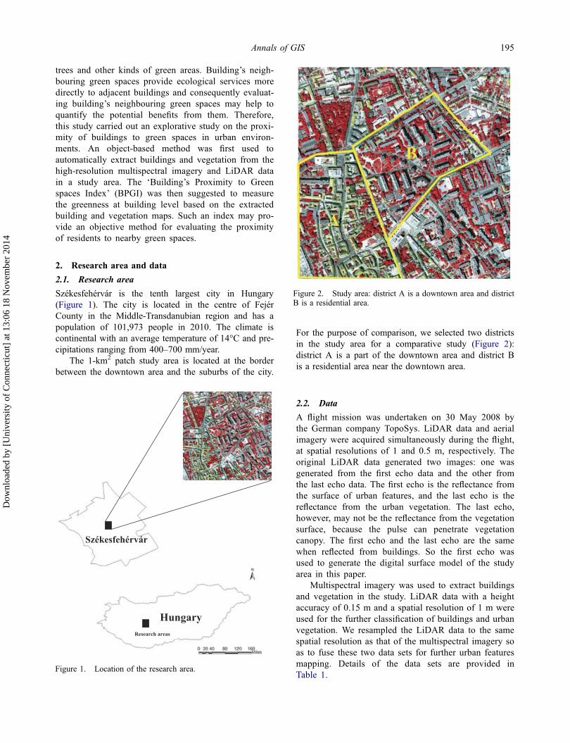
Székesfehérvár is the tenth largest city in Hungary(Figure 1). The city is located in the centre of FejérCounty in the Middle-Transdanubian region and has apopulation of 101,973 people in 2010. The climate iscontinental with an average temperature of 14°C and pre-cipitations ranging from 400–700 mm/year.

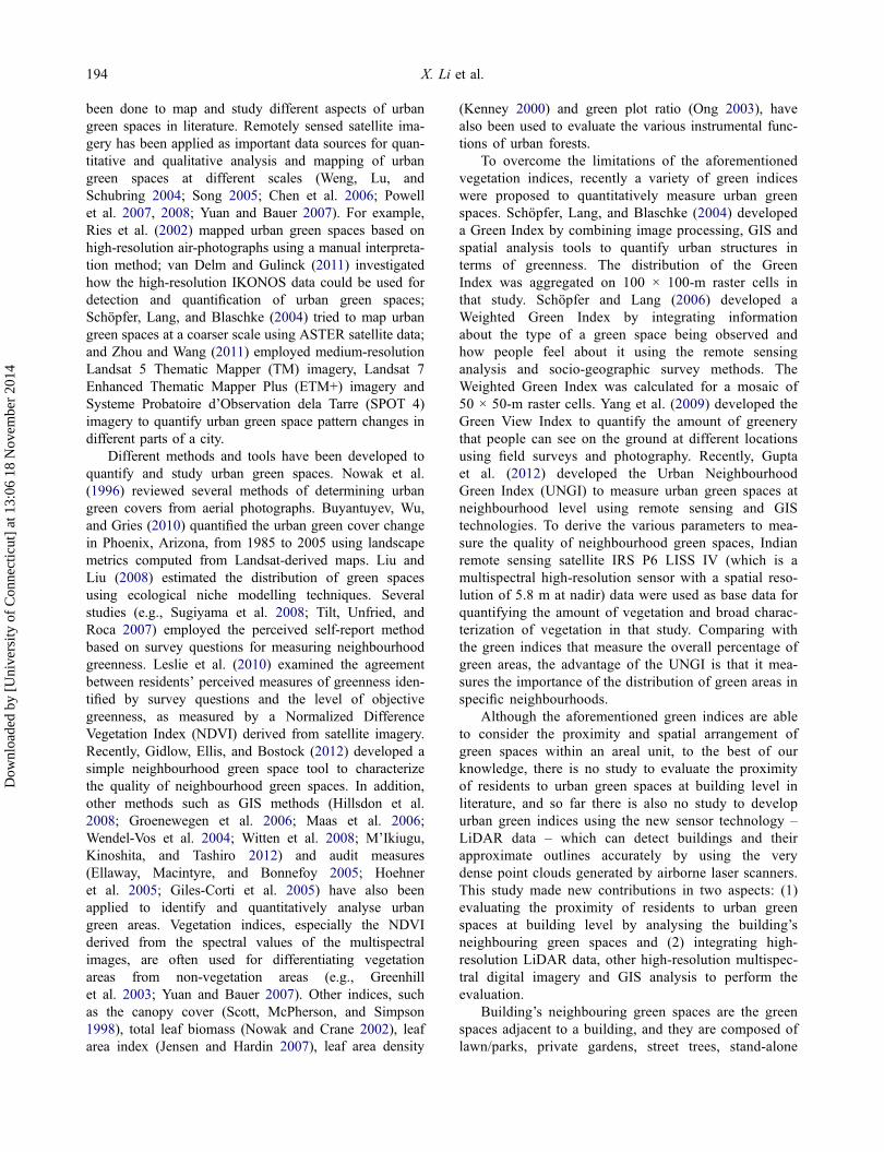
The 1-km2 patch study area is located at the borderbetween the downtown area and the suburbs of the city.

For the purpose of comparison, we selected two districtsin the study area for a comparative study (Figure 2):district A is a part of the downtown area and district Bis a residential area near the downtown area.

2.2. Data

A flight mission was undertaken on 30 May 2008 bythe German company TopoSys. LiDAR data and aerialimagery were acquired simultaneously during the flight,at spatial resolutions of 1 and 0.5 m, respectively. Theoriginal LiDAR data generated two images: one wasgenerated from the first echo data and the other fromthe last echo data. The first echo is the reflectance fromthe surface of urban features, and the last echo is thereflectance from the urban vegetation. The last echo,however, may not be the reflectance from the vegetationsurface, because the pulse can penetrate vegetationcanopy. The first echo and the last echo are the samewhen reflected from buildings. So the first echo wasused to generate the digital surface model of the studyarea in this paper.

Multispectral imagery was used to extract buildingsand vegetation in the study. LiDAR data with a heightaccuracy of 0.15 m and a spatial resolution of 1 m wereused for the further classification of buildings and urbanvegetation. We resampled the LiDAR data to the samespatial resolution as that of the multispectral imagery soas to fuse these two data sets for further urban featuresmapping. Details of the data sets are provided inTable 1.

HungaryResearch areas

Székesfehérvár

Figure 1. Location of the research area.

Figure 2. Study area: district A is a downtown area and districtB is a residential area.

Annals of GIS 195

Dow

nloa

ded

by [

Uni

vers

ity o

f C

onne

ctic

ut]

at 1

3:06

18

Nov

embe

r 20

14

3. Methodology

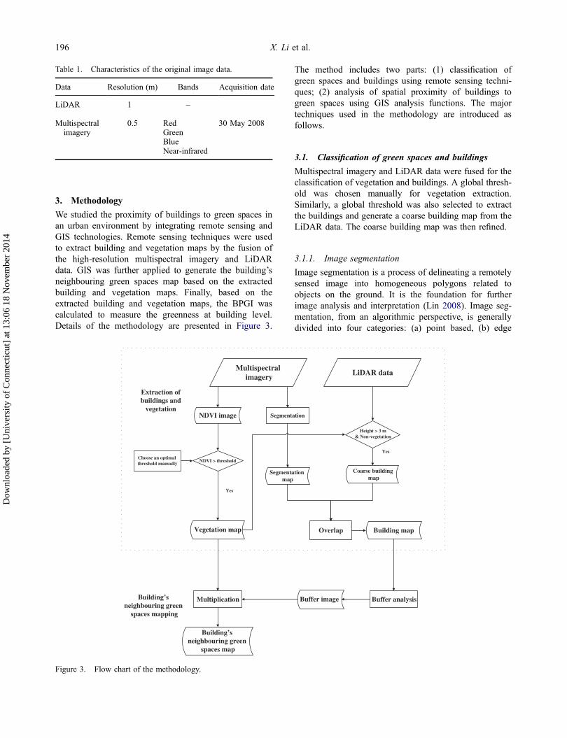
We studied the proximity of buildings to green spaces inan urban environment by integrating remote sensing andGIS technologies. Remote sensing techniques were usedto extract building and vegetation maps by the fusion ofthe high-resolution multispectral imagery and LiDARdata. GIS was further applied to generate the building’sneighbouring green spaces map based on the extractedbuilding and vegetation maps. Finally, based on theextracted building and vegetation maps, the BPGI wascalculated to measure the greenness at building level.Details of the methodology are presented in Figure 3.

The method includes two parts: (1) classification ofgreen spaces and buildings using remote sensing techni-ques; (2) analysis of spatial proximity of buildings togreen spaces using GIS analysis functions. The majortechniques used in the methodology are introduced asfollows.

3.1. Classification of green spaces and buildings

Multispectral imagery and LiDAR data were fused for theclassification of vegetation and buildings. A global thresh-old was chosen manually for vegetation extraction.Similarly, a global threshold was also selected to extractthe buildings and generate a coarse building map from theLiDAR data. The coarse building map was then refined.

3.1.1. Image segmentation

Image segmentation is a process of delineating a remotelysensed image into homogeneous polygons related toobjects on the ground. It is the foundation for furtherimage analysis and interpretation (Lin 2008). Image seg-mentation, from an algorithmic perspective, is generallydivided into four categories: (a) point based, (b) edge

Table 1. Characteristics of the original image data.

Data Resolution (m) Bands Acquisition date

LiDAR 1 –

Multispectralimagery

0.5 Red 30 May 2008GreenBlueNear-infrared

Building’s neighbouring green

spaces mapping

Multispectral imagery

LiDAR data

Coarse building map

Segmentation

Building map

NDVI image

Vegetation map

Height > 3 m& Non-vegetation

Choose an optimal threshold manually NDVI > threshold

Yes

Yes

Overlap

Buffer analysisBuffer imageMultiplication

Building’s neighbouring green

spaces map

Extraction of buildings and

vegetation

Segmentation map

Figure 3. Flow chart of the methodology.

196 X. Li et al.

Dow

nloa

ded

by [

Uni

vers

ity o

f C

onne

ctic

ut]

at 1

3:06

18

Nov

embe

r 20

14

based, (c) region based and (d) combined (Schiewe 2002).A region-based morphological tool for image segmenta-tion – the watershed transform (Vincent and Soille 1991) –was used in this study. Gradient magnitudes wereemployed prior to the watershed transform to preventover-segmentation (González, Woods, and Eddins 2009).Ideally, a watershed transform would result in a watershedridgeline or a segment line along the edge of an object.This characteristic allows the gradient-based watershedsegmentation method to correctly segment buildings withsharp contrasts at their edges.

The image segmentation procedure includes the fol-lowing steps: a gradient feature (i.e., root mean squarevalues of the horizontal and vertical grayscale gradientscalculated using a 3 × 3 Sobel operator) map was firstcalculated (Li et al. 2013). Then, it was segmented usinga moving threshold algorithm to obtain a marker image(Hill, Canagarajah, and Bull 2003), which was used todeal with the problem of over-segmentation. After trialand error, the optimum threshold was set to 5, becausethe segmentation result with this threshold coincidesvisually with the boundaries of urban features in theremotely sensed imagery. Before the watershed trans-form, the marker image was further used to reconstructthe gradient feature through a morphological method.The final step is to use the watershed algorithm revisedby Vincent and Soille (1991) to get the segmentationresult.

3.1.2. Green space extraction

The NDVI is the most widely used vegetation index. Itcan enhance the difference between vegetated and non-vegetated areas, due to the fact that vegetation displayshigh reflectance in the near-infrared band but has lowreflectance and high absorption in the red band. NDVI iscalculated as

NDVI ¼ NIR� RED

NIRþ RED(1)

where NIR is the reflectance in the near-infrared band andRED is the reflectance in the red band. In urban areas, theuse of NDVI can eliminate shadow effects and identifyshaded vegetation. Therefore, we did not consider shadowproblems when extracting vegetation.

Vegetation produces high values in an NDVI image,but non-vegetated areas have low values. An optimumthreshold of 0.23 was chosen manually after trial anderror for differentiating vegetated areas from non-vege-tated areas in the imagery. Vegetation density was notincluded in the classification process. The vegetationmap obtained by a pixel-based classification methodusually has a large number of ‘pepper and salt’ points.Based on empirical knowledge and field work, those

isolated vegetated areas with fewer than four pixels wereconsidered as misclassified locations and thus conse-quently were further classified into non-vegetated areas.In this study, because the spatial resolution of the vegeta-tion map is 0.5 m, the smallest area of vegetation that canbe delineated is 2 m2, which provides the ability to deline-ate a row of trees in a dense urban area. Although theneglect of vegetated areas smaller than four pixels maymiss some vegetation areas that still can provide ecologi-cal benefits, this effect should be negligible because suchsmall vegetation patches seldom occur near buildings.

3.1.3. Building extraction

Building roofs share the same spectral characteristics asroads and other impervious urban surfaces. It is, therefore,difficult to differentiate buildings from roads when usingonly multispectral imagery. The use of LiDAR data is anefficient way to extract buildings in urban areas. A thresholdof 3 m was used to extract high objects; that is, any featurewith a height below 3 m was not considered as a building.

A threshold method based on height cannot effec-tively differentiate urban buildings from trees. A vegeta-tion map was thus used to screen the green areas.Finally, the segmentation result was overlaid with thecoarse building map and a voting method was used todetermine the class of each object. We considered thewhole object to be a building if the percentage ofbuilding areas in an object was higher than 50%. Theupper part of Figure 3 shows the procedure of buildingextraction in detail.

3.2. Spatial proximity of buildings to green spaces

3.2.1. Generation of the building’s neighbouring greenspaces map

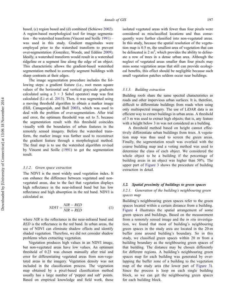
Building’s neighbouring green spaces refer to the greenspaces located within a certain distance from a building.Figure 4 illustrates the spatial arrangement of somegreen spaces and buildings. Based on the measurementfrom a remotely sensed image and the in situ investiga-tion, we found that most of building’s neighbouringgreen spaces in the study area are located in the 20-mbuffer zone around building’s boundary. So in thisstudy, we classified green spaces within 20 m from abuilding boundary as the neighbouring green spaces ofthat building. The distance may be chosen differentlyfor different regions. A building’s neighbouring greenspaces map for each building was generated by over-lapping the buffer zone of a building to the vegetationmap of the study area (the lower part of Figure 3).Since the process is loop on each single buildingblock, so we can get the neighbouring green spacesfor each building block.

Annals of GIS 197

Dow

nloa

ded

by [

Uni

vers

ity o

f C

onne

ctic

ut]

at 1

3:06

18

Nov

embe

r 20

14

3.2.2. The BPGI

Whitford, Ennos, and Handley (2001) pointed out thatthe greatest influence on ecological performance camefrom the percentage of green spaces. Therefore, in thisstudy, the BPGI is defined here as the ratio of theneighbouring green spaces area to the whole buffer area(excluding building area) of a building. Such a ratio isessentially a percentage (i.e., the percentage of the neigh-bouring green spaces accounting for the whole bufferarea of a building).

The BPGI for a building is calculated as

BPGIi ¼ BNGS areaiNon building areai

(2)

where BNGS_areai is the building’s neighbouring greenspaces area of the ith building (where i = 1 to n, and n is

the number of buildings in the research area), andNon_building_areai is the buffer area (excluding buildingarea) of the ith building. The upper and lower limits ofBPGI are 1.0 and 0, respectively. When there are noneighbouring green spaces in the buffer zone of a build-ing, its BPGI value is 0; on the contrary, when the bufferzone is fully filled with green spaces, the BPGI value ofthe building becomes 1.0. The higher the BPGI value is,the more proximity to nearby green spaces the build-ing has.

Such an index like the BPGI not only can measure thegreen spaces at the building level, but also may be used toassess the green spaces at the district or even city level.The mean or variance values of the BPGI in a specificdistrict or city may be used to indicate the greenness of theurban district or the whole city.

4. Results

4.1. Classification results

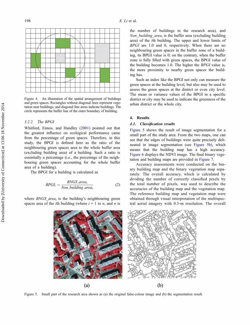
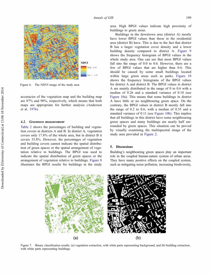
Figure 5 shows the result of image segmentation for asmall part of the study area. From the two maps, one cansee that the edges of buildings were quite precisely deli-neated in image segmentation (see Figure 5b), whichmeans that the building map has a high accuracy.Figure 6 displays the NDVI image. The final binary vege-tation and building maps are provided in Figure 7.

Accuracy assessments were conducted on the bin-ary building map and the binary vegetation map sepa-rately. The overall accuracy, which is calculated bydividing the number of correctly classified pixels bythe total number of pixels, was used to describe theaccuracies of the building map and the vegetation map.The reference building map and vegetation map wereobtained through visual interpretation of the multispec-tral aerial imagery with 0.5-m resolution. The overall

Figure 5. Small part of the research area shown as (a) the original false-colour image and (b) the segmentation result.

Figure 4. An illustration of the spatial arrangement of buildingsand green spaces. Rectangles without diagonal lines represent vege-tation near buildings, and diagonal line areas indicate buildings. Thecircle represents the buffer line of the outer boundary of building.

198 X. Li et al.

Dow

nloa

ded

by [

Uni

vers

ity o

f C

onne

ctic

ut]

at 1

3:06

18

Nov

embe

r 20

14

accuracies of the vegetation map and the building mapare 87% and 90%, respectively, which means that bothmaps are appropriate for further analysis (Andersonet al. 1976).

4.2. Greenness measurement

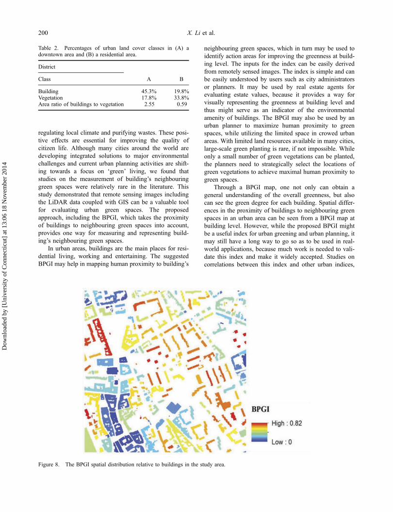
Table 2 shows the percentages of building and vegeta-tion covers in districts A and B. In district A, vegetationcovers only 17.8% of the whole area, but in district B itcovers 33.8%. However, the percentages of vegetationand building covers cannot indicate the spatial distribu-tion of green spaces or the spatial arrangement of vege-tation relative to buildings. The BPGI was used toindicate the spatial distribution of green spaces or thearrangement of vegetation relative to buildings. Figure 8illustrates the BPGI results for buildings in the study

area. High BPGI values indicate high proximity ofbuildings to green areas.

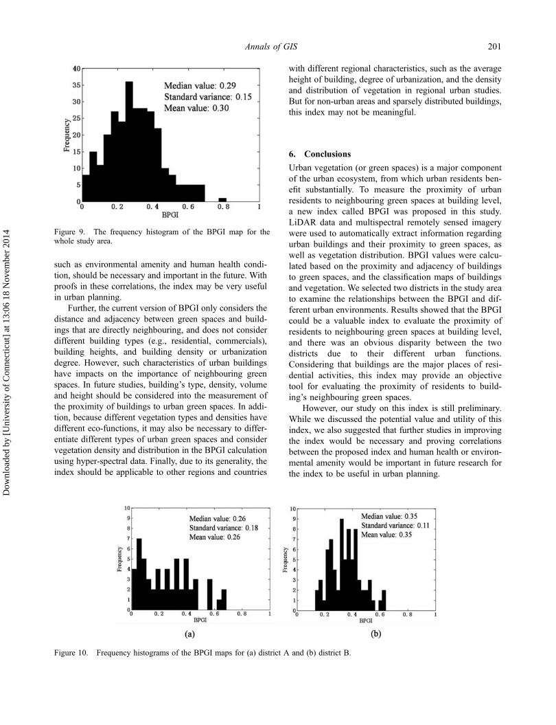
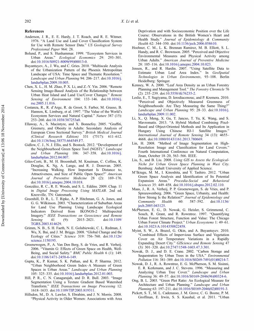
Buildings in the downtown area (district A) mostlyhave lower BPGI values than those in the residentialarea (district B) have. This is due to the fact that districtB has a larger vegetation cover density and a lowerbuilding density compared to district A. Figure 9shows the frequency histogram of BPGI values in thewhole study area. One can see that most BPGI valuesfall into the range of 0.0 to 0.6. However, there are afew of BPGI values that are higher than 0.6. Thisshould be caused by some small buildings locatedwithin large green areas such as parks. Figure 10shows the frequency histograms of the BPGI valuesfor district A and district B. The BPGI values in districtA are mainly distributed in the range of 0 to 0.6 with amedian of 0.26 and a standard variance of 0.18 (seeFigure 10a). This means that some buildings in districtA have little or no neighbouring green space. On thecontrary, the BPGI values in district B mostly fall intothe range of 0.2 to 0.6, with a median of 0.35 and astandard variance of 0.11 (see Figure 10b). This impliesthat all buildings in this district have some neighbouringgreen spaces and many buildings are nearly half sur-rounded by green spaces. This situation can be provedby visually examining the multispectral image of thestudy area provided in Figure 2.

5. Discussions

Building’s neighbouring green spaces play an importantrole in the coupled human-nature system of urban areas.They have many positive effects on the coupled system,such as mitigating noise pollution, increasing biodiversity,

Figure 6. The NDVI image of the study area.

Figure 7. Binary classification results: (a) vegetation extraction, with white parts representing background, and (b) building extraction,with white parts representing buildings.

Annals of GIS 199

Dow

nloa

ded

by [

Uni

vers

ity o

f C

onne

ctic

ut]

at 1

3:06

18

Nov

embe

r 20

14

regulating local climate and purifying wastes. These posi-tive effects are essential for improving the quality ofcitizen life. Although many cities around the world aredeveloping integrated solutions to major environmentalchallenges and current urban planning activities are shift-ing towards a focus on ‘green’ living, we found thatstudies on the measurement of building’s neighbouringgreen spaces were relatively rare in the literature. Thisstudy demonstrated that remote sensing images includingthe LiDAR data coupled with GIS can be a valuable toolfor evaluating urban green spaces. The proposedapproach, including the BPGI, which takes the proximityof buildings to neighbouring green spaces into account,provides one way for measuring and representing build-ing’s neighbouring green spaces.

In urban areas, buildings are the main places for resi-dential living, working and entertaining. The suggestedBPGI may help in mapping human proximity to building’s

neighbouring green spaces, which in turn may be used toidentify action areas for improving the greenness at build-ing level. The inputs for the index can be easily derivedfrom remotely sensed images. The index is simple and canbe easily understood by users such as city administratorsor planners. It may be used by real estate agents forevaluating estate values, because it provides a way forvisually representing the greenness at building level andthus might serve as an indicator of the environmentalamenity of buildings. The BPGI may also be used by anurban planner to maximize human proximity to greenspaces, while utilizing the limited space in crowed urbanareas. With limited land resources available in many cities,large-scale green planting is rare, if not impossible. Whileonly a small number of green vegetations can be planted,the planners need to strategically select the locations ofgreen vegetations to achieve maximal human proximity togreen spaces.

Through a BPGI map, one not only can obtain ageneral understanding of the overall greenness, but alsocan see the green degree for each building. Spatial differ-ences in the proximity of buildings to neighbouring greenspaces in an urban area can be seen from a BPGI map atbuilding level. However, while the proposed BPGI mightbe a useful index for urban greening and urban planning, itmay still have a long way to go so as to be used in real-world applications, because much work is needed to vali-date this index and make it widely accepted. Studies oncorrelations between this index and other urban indices,

Table 2. Percentages of urban land cover classes in (A) adowntown area and (B) a residential area.

District

A BClass

Building 45.3% 19.8%Vegetation 17.8% 33.8%Area ratio of buildings to vegetation 2.55 0.59

Figure 8. The BPGI spatial distribution relative to buildings in the study area.

200 X. Li et al.

Dow

nloa

ded

by [

Uni

vers

ity o

f C

onne

ctic

ut]

at 1

3:06

18

Nov

embe

r 20

14

such as environmental amenity and human health condi-tion, should be necessary and important in the future. Withproofs in these correlations, the index may be very usefulin urban planning.

Further, the current version of BPGI only considers thedistance and adjacency between green spaces and build-ings that are directly neighbouring, and does not considerdifferent building types (e.g., residential, commercials),building heights, and building density or urbanizationdegree. However, such characteristics of urban buildingshave impacts on the importance of neighbouring greenspaces. In future studies, building’s type, density, volumeand height should be considered into the measurement ofthe proximity of buildings to urban green spaces. In addi-tion, because different vegetation types and densities havedifferent eco-functions, it may also be necessary to differ-entiate different types of urban green spaces and considervegetation density and distribution in the BPGI calculationusing hyper-spectral data. Finally, due to its generality, theindex should be applicable to other regions and countries

with different regional characteristics, such as the averageheight of building, degree of urbanization, and the densityand distribution of vegetation in regional urban studies.But for non-urban areas and sparsely distributed buildings,this index may not be meaningful.

6. Conclusions

Urban vegetation (or green spaces) is a major componentof the urban ecosystem, from which urban residents ben-efit substantially. To measure the proximity of urbanresidents to neighbouring green spaces at building level,a new index called BPGI was proposed in this study.LiDAR data and multispectral remotely sensed imagerywere used to automatically extract information regardingurban buildings and their proximity to green spaces, aswell as vegetation distribution. BPGI values were calcu-lated based on the proximity and adjacency of buildingsto green spaces, and the classification maps of buildingsand vegetation. We selected two districts in the study areato examine the relationships between the BPGI and dif-ferent urban environments. Results showed that the BPGIcould be a valuable index to evaluate the proximity ofresidents to neighbouring green spaces at building level,and there was an obvious disparity between the twodistricts due to their different urban functions.Considering that buildings are the major places of resi-dential activities, this index may provide an objectivetool for evaluating the proximity of residents to build-ing’s neighbouring green spaces.

However, our study on this index is still preliminary.While we discussed the potential value and utility of thisindex, we also suggested that further studies in improvingthe index would be necessary and proving correlationsbetween the proposed index and human health or environ-mental amenity would be important in future research forthe index to be useful in urban planning.

Figure 9. The frequency histogram of the BPGI map for thewhole study area.

Figure 10. Frequency histograms of the BPGI maps for (a) district A and (b) district B.

Annals of GIS 201

Dow

nloa

ded

by [

Uni

vers

ity o

f C

onne

ctic

ut]

at 1

3:06

18

Nov

embe

r 20

14

ReferencesAnderson, J. R., E. E. Hardy, J. T. Roach, and R. E. Witmer.

1976. “A Land Use and Land Cover Classification Systemfor Use with Remote Sensor Data.” US Geological SurveyProfessional Paper 964: 28.

Bolund, P., and S. Hunhammar. 1999. “Ecosystem Services inUrban Areas.” Ecological Economics 29: 293–301.doi:10.1016/S0921-8009(99)00013-0.

Buyantuyev, A., J. Wu, and C. Gries. 2010. “Multiscale Analysisof the Urbanization Pattern of the Phoenix MetropolitanLandscape of USA: Time Space and Thematic Resolution.”Landscape and Urban Planning 94: 206–217. doi:10.1016/j.landurbplan.2009.10.005.

Chen, X. L., H. M. Zhao, P. X. Li, and Z.-Y. Yin. 2006. “RemoteSensing Image-Based Analysis of the Relationship betweenUrban Heat Island and Land Use/Cover Changes.” RemoteSensing of Environment 104: 133–146. doi:10.1016/j.rse.2005.11.016.

Costanza, R., R. d’Arge, R. de Groot, S. Farber, M. Grasso, B.Hannon, K. Limburg, et al. 1997. “The Value of the World’sEcosystem Services and Natural Capital.” Nature 387 (15):253–260. doi:10.1038/387253a0.

Ellaway, A., S. Macintyre, and X. Bonnefoy. 2005. “Graffiti,Greenery, and Obesity in Adults: Secondary Analysis ofEuropean Cross Sectional Survey.” British Medical Journal(Clinical Research Edition) 331 (7517): 611–612.doi:10.1136/bmj.38575.664549.F7.

Gidlow, C. J., N. J. Ellis, and S. Bostock. 2012. “Development ofthe Neighbourhood Green Space Tool (NGST).” Landscapeand Urban Planning 106: 347–358. doi:10.1016/j.landurbplan.2012.04.007.

Giles-Corti, B., M. H. Broomhall, M. Knuiman, C. Collins, K.Douglas, K. Ng, A. Lange, and R. J. Donovan. 2005.“Increasing Walking. How Important Is Distance to,Attractiveness, and Size of Public Open Space?” AmericanJournal of Preventive Medicine 28 (2): 169–176.doi:10.1016/j.amepre.2004.10.018.

González, R. C., R. E. Woods, and S. L. Eddins. 2009. Chap. 11in Digital Image Processing Using MATLAB. 2nd ed.Knoxville, TN: Gatesmark.

Greenhill, D. R., L. T. Ripke, A. P. Hitchman, G. A. Jones, andG. G. Wilkinson. 2003. “Characterization of Suburban Areasfor Land Use Planning Using Landscape EcologicalIndicators Derived from IKONOS-2 MultispectralImagery.” IEEE Transactions on Geoscience and RemoteSensing 41 (9): 2015–2021. doi:10.1109/TGRS.2003.814629.

Grimm, N. B., S. H. Faeth, N. E. Golubiewski, C. L. Redman, J.Wu, X. Bai, and J. M. Briggs. 2008. “Global Change and theEcology of Cities.” Science 319: 756–760. doi:10.1126/science.1150195.

Groenewegen, P., A. Van Den Berg, S. de Vries, and R. Verheij.2006. “Vitamin G: Effects of Green Space on Health, Well-Being, and Social Safety.” BMC Public Health 6 (1): 149.doi:10.1186/1471-2458-6-149.

Gupta, K., P. Kumar, S. K. Pathan, and K. P. Sharma. 2012.“Urban Neighborhood Green Index–A Measure of GreenSpaces in Urban Areas.” Landscape and Urban Planning105: 325–335. doi:10.1016/j.landurbplan.2012.01.003.

Hill, P. R., C. N. Canagarajah, and D. R. Bull. 2003. “ImageSegmentation Using a Texture Gradient Based WatershedTransform.” IEEE Transactions on Image Processing 12:1618–1633. doi:10.1109/TIP.2003.819311.

Hillsdon, M., D. A. Lawlor, S. Ebrahim, and J. N. Morris. 2008.“Physical Activity in Older Women: Associations with Area

Deprivation and with Socioeconomic Position over the LifeCourse: Observations in the British Women’s Heart andHealth Study.” Journal of Epidemiology & CommunityHealth 62: 344–350. doi:10.1136/jech.2006.058610.

Hoehner, C. M., L. K. Brennan Ramirez, M. B. Elliott, S. L.Handy, and R. C. Brownson. 2005. “Perceived and ObjectiveEnvironmental Measures and Physical Activity amongUrban Adults.” American Journal of Preventive Medicine28: 105–116. doi:10.1016/j.amepre.2004.10.023.

Jensen, R., and R. Hardin. 2007. “Using Satellite Data toEstimate Urban Leaf Area Index.” In GeoSpatialTechnologies in Urban Environments, 93–108. BerlinHeidelberg: Springer.

Kenney, W. A. 2000. “Leaf Area Density as an Urban ForestryPlanning and Management Tool.” The Forestry Chronicle 76(2): 235–239. doi:10.5558/tfc76235-2.

Leslie, E., T. Sugiyama, D. Ierodiaconouc, and P. Kremera. 2010.“Perceived and Objectively Measured Greenness ofNeighbourhoods: Are They Measuring the Same Thing?”Landscape and Urban Planning 95: 28–33. doi:10.1016/j.landurbplan.2009.11.002.

Li, X., Q. Meng, X. Gu, T. Jancso, T. Yu, K. Wang, and S.Mavromatis. 2013. “A Hybrid Method Combining Pixel-Based and Object-Oriented Methods and Its Application inHungary Using Chinese HJ-1 Satellite Images.”International Journal of Remote Sensing 34 (13): 4655–4668. doi:10.1080/01431161.2013.780669.

Lin, H. 2008. “Method of Image Segmentation on High-Resolution Image and Classification for Land Covers.”Fourth International Conference on Natural Computation,Jinan, October 18–20, 563–566. IEEE.

Liu, S., and B. Liu. 2008. Using GIS to Assess the Ecological-Niche for Urban Green Space Planning in Wuxi City.Bernburg: Anhalt University of Applied Science.

M’Ikiugu, M. M., I. Kinoshita, and Y. Tashiro. 2012. “UrbanGreen Space Analysis and Identification of Its PotentialExpansion Areas.” Procedia-Social and BehavioralSciences 35: 449–458. doi:10.1016/j.sbspro.2012.02.110.

Maas, J., R. A. Verheij, P. P. Groenewegen, S. de Vries, and P.Spreeuwenberg. 2006. “Green Space, Urbanity, and Health:How Strong Is the Relation?” Journal of Epidemiology andCommunity Health 60: 587–592. doi:10.1136/jech.2005.043125.

McPherson, E. G., D. Nowak, G. Heisler, S. Grimmond, C.Souch, R. Grant, and R. Rowntree. 1997. “QuantifyingUrban Forest Structure, Function and Value: The ChicagoUrban Forest Climate Project.” Urban Ecosystems 1: 49–61.doi:10.1023/A:1014350822458.

Myint, S. W., A. Brazel, G. Okin, and A. Buyantuyev. 2010.“Combined Effects of Impervious Surface and VegetationCover on Air Temperature Variations in a RapidlyExpanding Desert City.” GIScience and Remote Sensing 47(3): 301–320. doi:10.2747/1548-1603.47.3.301.

Nowak, D. J., and D. E. Crane. 2002. “Carbon Storage andSequestration by Urban Trees in the USA.” EnvironmentalPollution 116: 381–389. doi:10.1016/S0269-7491(01)00214-7.

Nowak, D. J., R. A. Rowntree, E. G. McPherson, S. M. Sisinni,E. R. Kerkmann, and J. C. Stevens. 1996. “Measuring andAnalyzing Urban Tree Cover.” Landscape and UrbanPlanning 36: 49–57. doi:10.1016/S0169-2046(96)00324-6.

Ong, B. L. 2003. “Green Plot Ratio: An Ecological Measure forArchitecture and Urban Planning.” Landscape and UrbanPlanning 63: 197–211. doi:10.1016/S0169-2046(02)00191-3.

Pickett, S. T., M. L. Cadenasso, J. M. Grove, C. G. Boone, P. M.Groffman, E. Irwin, S. S. Kaushal, et al. 2011. “Urban

202 X. Li et al.

Dow

nloa

ded

by [

Uni

vers

ity o

f C

onne

ctic

ut]

at 1

3:06

18

Nov

embe

r 20

14

Ecological Systems: Scientific Foundations and a Decade ofProgress.” Journal of Environmental Management 92: 331–362. doi:10.1016/j.jenvman.2010.08.022.

Powell, R., D. Roberts, P. Dennison, and L. Hess. 2007. “Sub-Pixel Mapping of Urban Land Cover Using MultipleEndmember Spectral Mixture Analysis: Manaus, Brazil.”Remote Sensing of Environment 106: 253–267.doi:10.1016/j.rse.2006.09.005.

Powell, S., W. Cohen, Z. Yang, J. Pierce, and M. Alberti. 2008.“Quantification of Impervious Surface in the SnohomishWaterResource Inventory Area of Western Washington from 1972–2006.” Remote Sensing of Environment 112: 1895–1908.

Ries, C., W. Pillmann, K. Kellner, and P. Stadler. 2002. “UrbanGreen Space Management Information Processing and Useof Remote Sensing Images and Scanner Data.” InProceedings of “Environmental Informatics” 2002, Part 1,503–510. Vienna: IGU/ISEP.

Rose, L. S., and R. Levinson. 2013. “Analysis of the Effect ofVegetation on Albedo in Residential Areas: Case Studies inSuburban Sacramento and Los Angeles, CA.” GIScience &Remote Sensing 50 (1): 64–77.

Schiewe, J. 2002. “Segmentation of High Resolution RemotelySensed Data Concepts, Applications and Problems.” In JointISPRS Commission IV Symposium: Geospatial Theory,Processing and Applications, July 9–12. CDROM.

Schöpfer, E., and S. Lang. 2006. “Finding the Right Shades ofUrban Greenery.” Accessed December 27, 2011. http://spie.org/x8749.xml

Schöpfer, E., S. Lang, and T. Blaschke. 2004. “A Green IndexIncorporating Remote Sensing and Citizen’s Perception ofGreen Space.” http://citeseerx.ist.psu.edu/viewdoc/sum-mary?doi=10.1.1.136.3035

Scott, K. I., E. G. McPherson, and J. R. Simpson. 1998. “AirPollutant Uptake by Sacramentos Urban Forest.” Journal ofArboriculture 24: 224–234.

Song, C. 2005. “Spectral Mixture Analysis for SubpixelVegetation Fractions in the Urban Environment: How toIncorporate Endmember Variability?” Remote Sensing ofEnvironment 95: 248–263. doi:10.1016/j.rse.2005.01.002.

Sugiyama, T., E. Leslie, B. Giles-Corti, and N. Owen. 2008.“Associations of Neighborhood Greenness with Physicaland Mental Health: Do Walking, Social Coherence andLocal Social Interaction Explain the Relationships?”Journal of Epidemiology and Community Health 62 (5), e9.

Tilt, J. H., T. M. Unfried, and B. Roca. 2007. “Using Objectiveand Subjective Measures of Neighborhood Greenness andAccessible Destinations for Understanding Walking Tripsand BMI in Seattle, Washington.” American Journal ofHealth Promotion 21 (4s): 371–379. doi:10.4278/0890-1171-21.4s.371.

van Delm, A., and H. Gulinck. 2011. “Classification andQuantification of Green in the Expanding Urban and Semi-Urban Complex: Application of Detailed Field Data andIKONOS-Imagery.” Ecological Indicators 11 (1): 52–60.doi:10.1016/j.ecolind.2009.06.004.

van Dillen, S. M. E., S. de Vries, P. P. Groenewegen, and P.Spreeuwenberg. 2012. “Greenspace in UrbanNeighbourhoods and Residents’ Health: Adding Quality toQuantity.” Journal of Epidemiology and Community Health66: e8–e8. doi:10.1136/jech.2009.104695.

Vincent, L., and P. Soille. 1991. “Watersheds in Digital Spaces:An Efficient Algorithm Based on Immersion Simulations.”IEEE Transactions on Pattern Analysis and MachineIntelligence 13: 583–598. doi:10.1109/34.87344.

Wendel-Vos, G. C. W., A. J. Schuit, R. de Niet, H. C.Boshuizen, W. H. M. Saris, and D. Kromhout. 2004.“Factors of the Physical Environment Associated withWalking and Bicycling.” Medicine and Science in Sportsand Exercise 36: 725–730. doi:10.1249/01.MSS.0000121955.03461.0A.

Weng, Q., D. Lu, and J. Schubring. 2004. “Estimation ofLand Surface Temperature–Vegetation AbundanceRelationship for Urban Heat Island Studies.” RemoteSensing of Environment 89: 467–483. doi:10.1016/j.rse.2003.11.005.

Westphal, L. M. 2003. “Social Aspects of Urban Forestry; UrbanGreening and Social Benefits: A Study of EmpowermentOutcomes.” Journal of Arboriculture 29: 137–147.

Whitford, V., A. R. Ennos, and J. F. Handley. 2001. “City Formand Natural Processes: Indicators for the EcologicalPerformance of Urban Areas and Their Application toMerseyside, UK.” Landscape Urban Planning 57 (2): 91–103. doi:10.1016/S0169-2046(01)00192-X.

Witten, K., R. Hiscock, J. Pearce, and T. Blakely. 2008.“Neighbourhood Access to Open Spaces and the PhysicalActivity of Residents: A National Study.” PreventiveMedicine 47: 299–303. doi:10.1016/j.ypmed.2008.04.010.

Wong, N. H., S. K. Jusuf, A. A. La Win, K. H. Thu, S. T.Negara, and W. Xuchao. 2007. “Environmental Study ofthe Impact of Greenery in an Institutional Campus in theTropics.” Building and Environment 42: 2949–2970.doi:10.1016/j.buildenv.2006.06.004.

Yang, F., Z. Y. Bao, and Z. J. Zhu. 2011. “An Assessment ofPsychological Noise Reduction by Landscape Plants.”International Journal of Environmental Research and PublicHealth 8: 1032–1048. doi:10.3390/ijerph8041032.

Yang, J., L. Zhao, J. Mcbride, and P. Gong. 2009. “Can You SeeGreen? Assessing the Visibility of Urban Forests in Cities.”Landscape and Urban Planning 91: 97–104. doi:10.1016/j.landurbplan.2008.12.004.

Yuan, F., and M. Bauer. 2007. “Comparison of ImperviousSurface Area and Normalized Difference Vegetation Indexas Indicators of Surface Urban Heat Island Effects in LandsatImagery.” Remote Sensing of Environment 106: 375–386.doi:10.1016/j.rse.2006.09.003.

Zhou, X., and Y. C. Wang. 2011. “Spatial–TemporalDynamics of Urban Green Space in Response to RapidUrbanization and Greening Policies.” Landscape andUrban Planning 100: 268–277. doi:10.1016/j.landurbplan.2010.12.013.

Annals of GIS 203

Dow

nloa

ded

by [

Uni

vers

ity o

f C

onne

ctic

ut]

at 1

3:06

18

Nov

embe

r 20

14