IEEE TGRS-2012-00997

1

Abstract— A Geophysical Model Function (GMF), denoted

XMOD2, is developed to retrieve sea surface wind field from X-band TerraSAR-X/TanDEM-X (TS-X/TD-X) data. In contrast to the previously developed XMOD1, XMOD2 consists of a nonlinear GMF, and thus, it depicts the difference between upwind and downwind of the sea surface backscatter in X-band SAR imagery. By exploiting 371 collocations with in situ buoy measurements which are used as the tuning dataset together with analysis wind model results, the retrieved TS-X/TD-X sea surface wind speed using XMOD2 shows a close agreement with buoy measurements with a bias of -0.32 m/s, an RMSE of 1.44 m/s and a scatter index (SI) of 16.0%. Further validation using an independent dataset of 52 cases shows a bias of -0.17 m/s, an RMSE of 1.48 m/s, and SI of 17.0% comparing with buoy measurements. To apply XMOD2 to TS-X/TD-X data acquired at HH polarisation, we validate three X-band SAR Polarisation Ratio (PR) models that were tuned using TS-X dual polarisation data by comparing the retrieved sea surface wind speed with buoy measurements.

Index Terms—Algorithm development, X-band SAR, sea surface wind

I. INTRODUCTION

HE spaceborne active microwave instruments of Scatterometer and Synthetic Aperture Radar (SAR) have

provided important marine-meteo parameters of the air-sea interface, particularly the sea surface wind speed at 10 m height ( 10U ) and the wind direction in high spatial resolution

and global coverage. Spaceborne SAR has a unique advantage to measure sea surface wind in spatial resolution higher than 1 km. This is especially important over coastal zones, where the sea surface wind field often exhibits significant spatial variation caused by coastal orography and man-made objects such as offshore wind turbines.

The general methodology to derive the sea surface wind field from SAR is to apply an empirical Geophysical Model Function (GMF) to the calibrated SAR image using wind direction from external sources or wind streaks visible in SAR imagery. The GMF relates the Normalized Radar Cross Section (NRCS, 0 ) to sea surface wind speed, wind direction

Manuscript received September 29, 2012; revised February 26, and April

21, 2013; accepted June 4, 2013. This work was supported in part by the EU-FP7 project “DOLPHIN” and in part by the German Federal Ministry of Education and Research (BMBF) project “MaMo” under grant of 03G0733A.

X.- M. Li and S. Lehner are with Remote Sensing Technology Institute of German Aerospace Center (DLR), Oberpfaffenhofen, 82234, Wessling, Germany (e-mail: Xiao.Li@dlr.de; Susanne.Lehner@dlr.de).

and incidence angle of radar. C-band (5.3 GHz) GMF families, e.g., the widely used CMOD4 [1], CMOD_IFR [2], CMOD5 [3] and CMOD5.N [4], are developed for the ERS Active Microwave Instrument (AMI) Scatterometer and the Advanced SCATterometer (ASCAT) to derive sea surface wind vectors over large swath with a spatial resolution of 25 km or 12.5 km. As scatterometers scan sea surface with fore-, mid- and aft- beams, a triple measurement depending only on wind speed and wind direction at a given node with known incidence angles is obtained. By collocating a large amount of reanalysis sea surface wind field data and/or in situ buoy measurements with scatterometer measurements, transfer functions in the GMF are subsequently derived, e.g., as presented in [5].

Since the ERS/SAR and ENVISAT/ASAR also operated in C-band, the CMOD functions are adapted to the C-band SAR data to map the sea surface wind field in high spatial resolution for different applications, e.g., meso-scale wind [6], katabatic wind [7], Bora events [8], coastal upwelling [9], and offshore wind farming [10]. As the CMOD functions are only available for radar data acquired at vertical polarisation (VV), to retrieve sea surface field from C-band SAR data at horizontal polarisation (HH), Polarisation Ratio (PR) models are proposed, e.g., by fitting airborne experimental data ([11] and [12]) or based on sea surface backscatter theory [13]. The sea surface backscatter in HH polarisation HH

0 is converted to VV0 by using PR models, and then the CMOD functions are

applied to retrieve sea surface wind. These PR models are further verified or adjusted by comparing the retrieved RADARSAT-1 SAR sea surface wind speed with scatterometer and/or in situ buoy measurements ([14] – [16]). Apart from these models which consider only the effect of incidence angle on polarisation ratios, PR models including additional influences of wind direction ([12]) and wind speed ([17]) on polarisation ratios are also proposed, which yield a better conversion of HH

0 to VV0 .

The CMOD functions are shown to be suitable for retrieving sea surface wind field from C-band SAR sensors. However, a new GMF has to be developed when SAR operates at different microwave frequencies, such as the ALOS/PALSAR in L-band (1.2 GHz), the TerraSAR-X/Tandem-X (TS-X/TD-X) and the Cosmo-Skymed in X-band (9.6 GHz). As a SAR has one antenna instead of several ones like for scatterometers, a feasible approach of deriving a suitable GMF is to match up SAR measurements with externally derived wind vectors, e.g. presented in [18] for an L-band GMF to retrieve sea surface wind from ALOS/PALSAR.

Algorithm for sea surface wind retrieval from TerraSAR-X and TanDEM-X data

Xiao-Ming Li, and Susanne Lehner, Member, IEEE

T

brought to you by COREView metadata, citation and similar papers at core.ac.uk

provided by Institute of Transport Research:Publications

IEEE TGRS-2012-00997

2

Recently, more attention is being brought to the use of TS-X/TD-X and Cosmo-SkyMed data for coastal monitoring as they can provide observations with high spatial resolution, as well in a constellation configuration. Further, retrieval of sea surface wind field is one promising application of SAR for operational weather services. Therefore, in the present study, we focus on algorithm development of sea surface wind retrieval from TS-X and TD-X data.

Our first algorithm, called XMOD1 [19], was developed using a linear GMF to retrieve sea surface wind from X-band SAR data, which was tuned using the SIR-X SAR data. The PR models describing the dependence of PR on incidence angle proposed by Thompson et al. [11] and Elfhouhaily et al. [13] were retuned using TS-X dual-polarisation data [20]. Additionally, in the study of [20], an exponential type of PR model called X-PR, which is similar with the model given by Mouche et al. [12], is proposed to retrieve sea surface wind speed from the TS-X/TD-X data at HH polarisation. Thompson et al. [21] also propose an empirical algorithm by interpolating the NRCS values between C-band and Ku-band to X-band for retrieving sea surface wind speed from TS-X data at both VV and HH polarisations.

Following the Introduction, in Section II, the dataset used in the present study is briefly described. The methodology to develop the GMF, called XMOD2 hereafter, for sea surface wind field retrieval from TS-X/TD-X data at VV polarisation is described in detail in Section III. In Section IV, we present simulation and validation of XMOD2. Following that, application of XMOD2 on TS-X/TD-X data at HH polarisation using the three tuned PR models is described in Section V. Discussion and Conclusions are given in the last section.

II. DATA SET

A. TS-X and TD-X data

The TS-X and TD-X satellites can image in Spotlight, Stripmap and ScanSAR modes as well as in multiple combinations of polarisations. In the present study, we used the Stripmap and ScanSAR mode data acquired at co-polarisation (VV or HH) to retrieve sea surface wind. Stripmap data have a pixel size of 2.5 m and a swath of around 30 km, and the ScanSAR mode can provide images at large coverage of 100 km with a pixel size of 8.25 m.

TS-X/TD-X Stripmap data constitute a majority of the dataset used for the tuning of XMOD2. In addition, there are a few ScanSAR data are included in the tuning dataset. For Stripmap data, an absolute radiometric calibration accuracy of 0.31 dB was achieved during the commissioning phase [22]. After two years of its launch, the recalibration results [23] show that TS-X still works very successfully with an absolute radiometric accuracy of 0.34 dB. The Noise Equivalent Sigma Zero (NESZ) of TS-X and TD-X data lies between -19 dB and -26 dB, depending on the variation of incidence angles (i.e., the antenna beam pattern), and the average value is approximately −21 dB [24].

B. In situ buoy measurements

1) Correction of buoy wind speed For tuning and validation of XMOD2, in situ buoy

measurements are accessed from the National Data Buoy Center (NDBC), USA and the Integrated Science Data Management (ISDM), Canada. The continuous wind data of the NDBC buoys are available every 10 minutes, while the accessed wind measurements of the Canadian buoys are available hourly. Anemometers on most buoys are mounted at 5 m height above the sea surface. However, wind measurements derived from microwave sensors, e.g., scatterometry, radiometry and SAR, are at a standard height of 10 m above the sea surface. Therefore, wind speed measured by anemometers at different heights is corrected to the reference level of 10 m height for comparisons with satellite measurements. In this work, we used two methods for wind speed corrections. The first method of correcting the wind speed mzU at a height of mz measured by buoy to the wind

speed at 10 m height zU is to use a simple logarithmical varying wind profile, as given in (1).

00 lnln zzzzzUzU mm (1)

Where 0z is the roughness length, which has a typical value of

1.52 × 10-4 [25]. This expression is derived using a mixing length approach assuming neutral stability [25], i.e., neglecting the effect of differences in atmospheric stability, which, therefore, may lead to errors when atmospheric conditions are different from neutral stability. The corrected wind speed to 10 m height using this method is called LOGU

hereafter. The second method is to correct the buoy measured wind

speed to the equivalent neutral wind at 10 m height using the LKB method proposed in [26]. In the LKB method, the buoy measured wind speed is transformed to surface stress by taking into account the atmospheric stability between buoy observation height and the sea surface. Then the equivalent neutral wind is obtained by transforming the surface stress back to 10 m height without considering the stability effects. Thus, such winds are considered to be measurements of wind stress expressed in units of wind speed. The corrected buoy wind speed using this method is called LKBU hereafter.

Both scatterometer and SAR transmit pulses to the sea surface and therefore respond directly to the sea surface roughness rather than the 10 m wind, which is closely associated with the wind stress. Therefore, the LKB method is considered to be more reasonable to correct buoy measurements, as it provides a wind speed for a given wind stress that would be observed at a height of 10 m assuming a neutrally stable atmosphere. This method has been widely used to correct buoy wind measurements to 10 m height for comparison with satellite-derived wind measurements, e.g., from the radiometer of SSM/I [27] and the scatterometers of NSCAT and QuikSCAT [28].

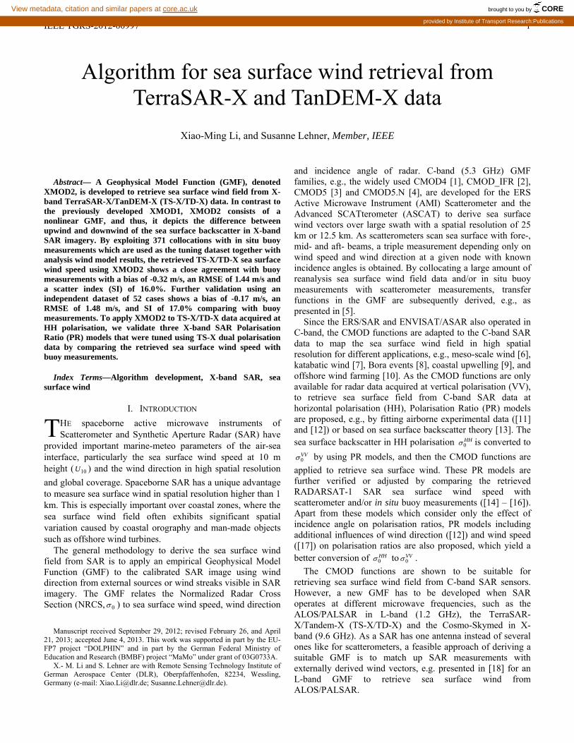
In Fig. 1, we show the comparison between the corrected wind speed using the two methods described above. The comparison indicates that LKBU is slightly higher than LOGU

by 0.21 m/s, which is consistent with the finding in [27].

IEEE TGRS-2012-00997

3

Fig.1. Comparison of corrected wind speed at 10 m height using the LOG and LKB methods.

2) Matchup of TS-X/TD-X data with buoy measurements

TS-X/TD-X acquisitions are spatially and temporally

matched up to in situ buoy measurements. At the locations of the buoys, the mean sea surface backscatter 0 and the local

incidence angle are extracted from TS-X/TD-X subscenes with coverage of 2 km × 2 km, which are subsequently collocated with buoy measurements.

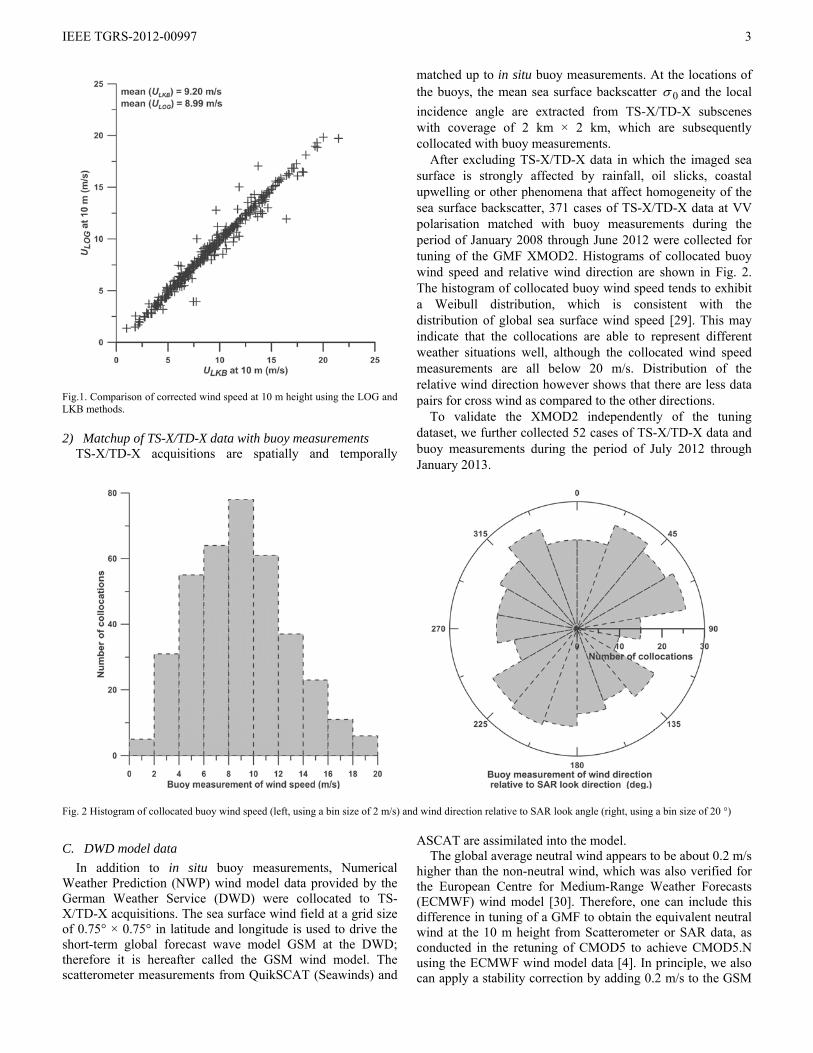
After excluding TS-X/TD-X data in which the imaged sea surface is strongly affected by rainfall, oil slicks, coastal upwelling or other phenomena that affect homogeneity of the sea surface backscatter, 371 cases of TS-X/TD-X data at VV polarisation matched with buoy measurements during the period of January 2008 through June 2012 were collected for tuning of the GMF XMOD2. Histograms of collocated buoy wind speed and relative wind direction are shown in Fig. 2. The histogram of collocated buoy wind speed tends to exhibit a Weibull distribution, which is consistent with the distribution of global sea surface wind speed [29]. This may indicate that the collocations are able to represent different weather situations well, although the collocated wind speed measurements are all below 20 m/s. Distribution of the relative wind direction however shows that there are less data pairs for cross wind as compared to the other directions.

To validate the XMOD2 independently of the tuning dataset, we further collected 52 cases of TS-X/TD-X data and buoy measurements during the period of July 2012 through January 2013.

Fig. 2 Histogram of collocated buoy wind speed (left, using a bin size of 2 m/s) and wind direction relative to SAR look angle (right, using a bin size of 20 °)

C. DWD model data

In addition to in situ buoy measurements, Numerical Weather Prediction (NWP) wind model data provided by the German Weather Service (DWD) were collocated to TS-X/TD-X acquisitions. The sea surface wind field at a grid size of 0.75° × 0.75° in latitude and longitude is used to drive the short-term global forecast wave model GSM at the DWD; therefore it is hereafter called the GSM wind model. The scatterometer measurements from QuikSCAT (Seawinds) and

ASCAT are assimilated into the model. The global average neutral wind appears to be about 0.2 m/s

higher than the non-neutral wind, which was also verified for the European Centre for Medium-Range Weather Forecasts (ECMWF) wind model [30]. Therefore, one can include this difference in tuning of a GMF to obtain the equivalent neutral wind at the 10 m height from Scatterometer or SAR data, as conducted in the retuning of CMOD5 to achieve CMOD5.N using the ECMWF wind model data [4]. In principle, we also can apply a stability correction by adding 0.2 m/s to the GSM

IEEE TGRS-2012-00997

4

wind data to tune a neutral wind GMF for X-band SAR data. However, sea surface temperature, sea level pressure, humidity and air temperature are not provided in the GSM wind model, it is not possible to verify whether the differences (0.2 m/s) is also applicable for the GSM model. Therefore, in this work, we use the GSM real wind at 10 m height and the corrected buoy measurements LOGU to tune XMOD2.

III. METHODOLOGY

Following the description of dataset used in this study, development of the GMF XMOD2 is presented in detail.

A. Comparison of the sea surface backscatter in X-, C- and Ku-band

The microwave frequency of X-band TS-X/TD-X is 9.65 GHz, which lies between C-band (5.33 GHz) and Ku-band (13.99 GHz). Therefore, it is considered that 0 in X-band

data should be close to that in both C-band and Ku-band data, which is also the principle of [21] to empirically derive an X-band GMF by interpolating the C-band and Ku-band NRCS. Therefore, in this work, we first compare the 0 measured by

TS-X/TD-X, denoted TSX0 , with the simulated one using the

GMF of CMOD5.N and NSCAT1 [31] for C-band and Ku-band radar at VV polarisation, which is denoted CSim _

0 andKuSim _

0 , respectively. Buoy measurements of wind direction,

corrected wind speed at 10 m height (i.e., equivalent neutral wind speed LKBU ) and local incidence angles of the TS-X/TD-X subscenes at buoy locations are input to the two GMFs to obtain a simultaneous measurement of NRCS in C- and Ku-

band with X-band observation. The comparisons are shown in Fig. 3. The red dashed curves in Fig. 3 are polynomial fitting between the observed X-band NRCS and simulated C-band or Ku-band NRCS.

Since radar backscatter of the sea surface is dominated by the Bragg resonant scattering, the discrepancy of simultaneous NRCS in C-, X-, and Ku-band should be comparable as microwave frequency of X-band is in the middle of C- and Ku-band. However, it is surprising that the difference between

TSX0 and KuSim _

0 is only -0.02 dB, which is much smaller than

the difference of 0.89 dB between TSX0 and CSim _

0 .

The other interesting finding in the two comparisons is the variation of agreement between the polynomial fitting and the identity line. Referring to NRCS measurements of TS-X/TD-X, measured TSX

0 is higher than both CSim _0 and KuSim _

0 in

the range of around -22.5 dB and -12.5 dB. For NRCS of TS-X/TD-X varies between -12.5 dB and -5 dB, TSX

0 is slightly

higher than CSim _0 , while it is slightly lower than KuSim _

0 . If

NRCS is above -5 dB, TSX0 is still larger than CSim _

0 and the

difference shows a tendency of increasing with NRCS. However, in the same range, TSX

0 is nearly equal to KuSim _0 .

Since the primary goal of the present study is to develop a GMF for X-band TS-X/TD-X to retrieve sea surface wind, these findings remain our further investigations, in particular by classifying them to difference wind speed, wind direction and incidence angle after acquiring more collocations of TS-X/TD-X with in situ buoy measurements.

Fig.3 Comparisons of 0 measured by TS-X/TD-X with that simulated for C- (left) and Ku-band (right) radars.

B. Development of the GMF XMOD2 for TS-X/TD-X data

1) Derivation of XMOD2 As the currently available TS-X/TD-X collocations with

other datasets, such as in situ buoy measurements and scatterometer measurements, are not sufficient to derive transfer functions independently by fitting the observed TSX

0

to measured sea surface wind speed and wind direction. To

IEEE TGRS-2012-00997

5

overcome this problem, we introduce a practical approach to develop a GMF for TS-X and TD-X data.

The comparisons shown in Fig. 3 indicate that 0 observed

by X-band radar is in close agreement with that by both C- and Ku-band radars, particularly with Ku-band. However, a twofold consideration leads us to adopt the model functions of CMOD5 to X-band SAR data. The C-band GMF has been widely used for retrieving the sea surface wind field from C-band SAR data; on the other hand, CMOD5 is particularly developed for a good retrieval of the sea surface wind field in both low and high wind speed. Although the current tuning dataset for X-band GMF includes only a few cases acquired in high wind speed (above 20 m/s), the adoption of CMOD5 to X-band SAR gives a possibility for further tuning of X-band GMF for high wind speed.

The CMOD5 is written as:

2cos,cos,1,,, 210 vBvBvBvz p (2)

where ,0B ,1B and 2B are functions of incidence angle and

the sea surface wind speed v at 10 m height. Relative direction is the angle between wind direction and radar look direction , i.e. . p is a constant with value of 0.625. In CMOD5, the isotropic term 0B , the

upwind/downwind amplitude 1B and upwind/crosswind amplitude 2B are all the functions of wind speed and incidence angle.

In GMFs, the 0B and 2B terms dominate the relation

between sea surface backscatter with wind vector and incidence angle. Therefore, in the proposed GMF XMOD2 for X-band SAR, transfer functions used to depict 0B and 2B are

adopted from CMOD5, while a second-order polynomial function is used to describe the dependence of 1B on the sea surface wind speed and incidence angle as given in (3).

2

0

2

01

j i

jiij vaB (3)

2) Tuning Approach A stepwise regression is used in the tuning approach. First,

it is assumed that the observed sea surface backscatter TSX0 is

only related to the sea surface wind speed and incidence angle, i.e.

,00 vB pTSX (4)

Coefficients in 0B are tuned by minimizing the following

cost function:

N

iii

pTSXi vBBJ

1000cost , (5)

Neglecting the difference of the upwind and downwind onTSX0 , i.e. only considering the difference in upwind and

crosswind, TSX0 approximates to be,

2cos,1, 200 vBvB pTSX (6)

As the coefficients of 0B have been determined via (5), (6)

is rewritten as,

2cos,1, 2000 vBvB pTSX (7)

Again, the least mean square method (5) is used to determine the coefficients for the transfer functions in 2B . Consequently, the coefficients for the functions in 1B are determined as well when the difference of upwind and downwind on sea surface backscatter in X-band SAR image is considered.

As shown in Fig. 2, the collocated buoy measurements are irregularly distributed, particularly for wind direction. However, the TS-X/TD-X data over buoys are acquired individually and are the all available collocations at this time since the starting of operational phase of TS-X in December 2007. Therefore, while acquiring future data, for now, we have to consider additional collocations to further consolidate the tuning dataset.

In the tuning approach described above, coefficients in the GMF for X-band data are preliminary determined by collocations of TS-X/TD-X data and buoy measurements. The preliminary GMF is called XMOD_internal. By applying the XMOD_internal to collocations of TS-X/TD-X data and the GSM wind model results, one obtains a simulated sea surface backscatter which is denoted DWDsim _

0 . If the difference

between the DWDsim _0 and the SAR measurements TSX

0 is less

than an empirical threshold of 2 dB, the collocations are then selected for fine tuning of XMOD2. The threshold is set to exclude some spurious model data which may induce significant discrepancies between the simulated 0 and the

SAR measurements. After this procedure, there are 639 collocated pairs of the TS-X/TD-X and DWD model results that are selected for further tuning. 95% of the collocated GSM wind model data are 100 km away from the coast. Finally, a total of 1010 collocations of TS-X/TD-X data with in situ buoy measurements and the GSM model results are used as the tuning dataset. Fig. 4 shows the histograms of wind speed and wind direction of the tuning dataset. Comparing Fig. 4 to Fig. 2, one can find that adding collocations the GSM wind model results overcomes the problem of irregular sampling to some extent.

Coefficients in XMOD2 are determined by repeating the steps given in (4) – (7) using the mixed tuning dataset, which are listed in Appendix. XMOD2 is applicable for X-band SAR data acquired with incidence angles between 20° and 45° and at VV polarisation. Note that the tuned XMOD2 does not yield the equivalent neutral winds, but the real winds at 10 m height.

IV. SIMULATION AND VALIDATION OF THE XMOD2

A. Simulation

Fig. 5 shows the simulated 0 using XMOD2 against

relative wind direction in the sea surface wind speed of 10 m/s for incidence angles of 20°, 30° and 40°, respectively. The simulation shows that XMOD2 can represent properly the anisotropic effect of wind direction on the sea surface backscatter. Moreover, the incidence angle effect on the difference between upwind and crosswind, as well as on that

IEEE TGRS-2012-00997

6

between upwind and downwind, are also distinct. One can find that the higher the incidence angle, the more sensitive 0 is on

the sea surface wind direction.

Fig. 4 Histogram of collocated buoy measurements and GSM model wind speed (left, using a bin size of 2 m/s) and wind direction relative to SAR look angle (right, using a bin size of 20°)

Fig. 5 Simulated sea surface backscatter using XMOD2 against relative wind direction for incidence angles of 20°, 30° and 40°, respectively, in the sea surface wind speed of 10m/s. The red lines present the same simulations but using CMOD5 for C-band radar data.

Fig. 6 (a) and (b) show the simulated sea surface

backscatter using XMOD2 for incidence angles of 20°, 30° and 40° in upwind and crosswind. In both Fig.5 and Fig.6, the same simulations for C-band radar using CMOD5 are also presented for comparison with. With respect to Fig. 5, the simulation shows that the difference between X- and C-band increases with incidence angle, particularly for upwind and cross wind. In Fig. 6, it is interesting to notice that, for

upwind, the transition of the difference between X-band and C-band 0 shows a dependence on the sea surface wind

speed. For incidence of 20°, 30°, and 40°, the transition appears at around 8 m/s, 6 m/s and 4 m/s, respectively. However, in cross wind, the simulated X-band 0 is generally

larger than that of C-band without independence on the sea surface wind speed.

Another issue that we investigate is the usability of XMOD2 to retrieve low wind speed from TS-X/TD-X data. NESZ is a measurement of the sensitivity of a radar system to areas of low backscatter, which is an important parameter to assess quality of the SAR data. The NESZ of TS-X/TD-X data used in the tuning dataset is derived from the XML file, which is shown as a function of incidence angle in Fig. 7. Note that the NESZ in one TS-X/TD-X scene varies along with incidence angle. Considering that variation of incidence angle of TS-X/TD-X Stripmap data is relative small (about 2.5°), we use the averaged NESZ and incidence angle over one scene for representation. The overall NESZ of TS-X/TD-X data used in the tuning dataset is -22.06 dB. The simulated TS-X/TD-X 0 under wind speeds of 1 m/s, 2 m/s and 5 m/s in

crosswind is shown as well in the figure. For the sea surface wind speed above 2 m/s, the simulated 0 is higher than the

NESZ for all incidence angles. Only when incidence angle is steeper than 30°, the simulated 0 for a sea surface wind speed

of 1 m/s is larger than the NESZ. This indicates that 2 m/s is the minimum wind speed that one can retrieve using XMOD2 for incidence angles between 20° and 45°. If the incidence angle is steeper than 30°, a lower sea surface wind speed of 1 m/s can be retrieved as well.

IEEE TGRS-2012-00997

7

(a) (b)

Fig.6 Simulated sea surface backscatter using XMOD2 for incidence angles of 20°, 30° and 40° against the sea surface wind speed in upwind (a) and crosswind (b). The red lines present the same simulations but using CMOD5 for C-band radar data.

Fig. 7. Comparison of the NESZ derived from the TS-X/TD-X data used in

the tuning dataset with the simulated 0 using XMOD2 in cross wind for a

wind speed of 1 m/s, 2 m/s and 5 m/s, respectively.

B. Validation

In the validation exercises, we focus on the comparison of the retrieved TS-X/TD-X sea surface wind speed with in situ buoy measurements. To retrieve the SAR sea surface wind speed using GMFs, accurate information of wind direction has to be obtained as a priori. In other words, it is difficult to verify GMFs if errors of the retrieved wind speed are additionally induced by uncertainty of wind direction. Therefore, buoy measured wind direction, which is considered to be the best observations close to ground truth, is used as input to XMOD2 to derive the TS-X/TD-X wind speed for validating XMOD2.

It is no doubt that the larger the amount of accurate measurements is used, such as derived from in situ buoys, the better XMOD2 can be tuned. However, if all the available

buoy collocations are already used for tuning, validation will lack an important dataset, thus one has to consider the trade-off between the tuning and validation dataset. As the primary goal of the present study is to construct a suitable GMF to retrieve the sea surface wind field from TS-X/TD-X data, we use all the collocations with buoy measurements from starting of the operational phase of TS-X in December, 2007 till June, 2012 for tuning XMOD2. On the other hand, in order to reduce irregular distributions of wind speed and wind direction in the tuning dataset, a large amount of GSM wind model results, which is nearly twice that of the collocations with buoy measurements, is further added to the tuning dataset. Therefore, comparison of the retrieved sea surface wind speeds to buoy measurements is still necessary to verify XMOD2. The comparison in Fig. 8 shows that the retrieved TS-X/TD-X wind speed is in good agreement with buoy measurements with a bias of -0.32 m/s, a RMSE of 1.47 m/s and a Scatter Index (SI) of 16.0% for the sea surface wind speed in the range of 2 m/s to 20 m/s. Note that a centered RMSE [32] is used for evaluating quality of the retrieved sea surface wind speed in this study, though it is still called RMSE hereafter.

Parallel with the development of XMOD2, we also obtained TS-X/TD-X acquisitions over NDBC and Canadian buoys to get an independent dataset to validate XMOD2. Fig. 9 shows the comparison of the retrieved sea surface wind speed from TS-X/TD-X data acquired during July 2012 through January 2013 with in situ buoy measurements. This comparison using an independent dataset shows a bias of -0.17 m/s, an RMSE of 1.48 m/s and a SI of 17.0%, which are all consistent with those achieved in the comparison using the tuning dataset.

Development and validation of XMOD2 for TS-X/TD-X data at VV polarisation are described above. Its application on TS-X/TD-X data at HH polarisation is presented in the next section.

IEEE TGRS-2012-00997

8

Fig. 8. Comparison of the retrieved TS-X/TD-X sea surface wind speed using XMOD2 against in situ buoy measurements that are used in the tuning dataset (December 2007 to June 2012).

Fig. 9. Comparison of the retrieved TS-X/TD-X sea surface wind speed using XMOD2 against in situ buoy measurements that not included in the tuning dataset (July 2012 to January 2013).

V. APPLICATION OF XMOD2 ON TS-X/TD-X DATA AT HH

POLARISATION

In a recent study, we develop three models [19] depicting the dependence of TS-/TD-X Polarisation Ratio (PR) on incidence angle. The PR models are used to convert NRCS of HH polarisation ( HH

0 ) data to that of VV polarisation data (VV0 ) in order to retrieve the sea surface wind speed from TS-

X/TD-X data at HH polarisation using the developed GMF dedicated for VV polarisation data. Among the three models, two (i.e., the Thompson Model [11] and the Elfouhaily Model [13], denoted T-PR and E-PR, respectively) are based on the

models which are originally proposed for C-band SAR data and the third one (X-PR) is derived according to the GMF for X-band airborne scatterometer [33]. Coefficients of the three PR models are determined using TS-X dual-polarisation data. The T-PR and the exponential X-PR models are given in (8) and (9), respectively.

22

22

0

0

)tan1(

)tan21(T_PR

HH

VV (8)

)exp(X_PR 10 XX (9)

Coefficients of for (8), and 10, XX for (9) tuned using TS-

X dual polarisation data are given in [20]. They are also listed in Table I for reference.

TABLE I

COEFFICIENTS OF THE PR MODELS TUNED FOR TS-X/TD-X

PR models Coefficients

T-PR model 1.65

X-PR model 0X 0.61

1X 0.02

The E_PR model is based on the Extended Kirchhoff

Approximation (EKA) model [13]. We find that the E_PR model does not fit for the TS-X dual polarisation data in the

original format 022

220

)tan21(

)sin21(VVHH

; therefore, we modify

the coefficient in it by fitting the PR derived from the TS-X dual polarisation data [20], which has the following format:

22

22

0

0

)sin65.21(

)tan21(

HH

VVPRE (10)

60 TS-X/TD-X SAR images acquired between 2008 and 2012 at HH polarisation are collected and matched up to the in situ buoy measurements. We use the three proposed PR models and XMOD2 to retrieve the TS-X/TD-X sea surface wind speed and compare them with in situ buoy measurements, as shown in Fig.10. Overall, the three PR models yield bias larger than 0.5 m/s and RMSE larger than 2.0 m/s. The T_PR yields the best bias of -0.64 m/s, but the largest RMSE and SI. The modified E_PR shows the largest bias of -0.93 m/s. Although the bias (-0.88 m/s) achieved by using the X_PR model is slightly larger than that using the T_PR model, the X_PR model yields the best RMSE and SI, with value of 2.03 m/s and 22.4%, respectively. Therefore, we preliminarily conclude that the proposed X_PR model performs best among the three PR models.

In Fig.11, we show an example of the sea surface wind field retrieved using XMOD2 and X_PR model for a TS-X dual-polarisation (VV and HH) acquired over the Diamond Shoals, USA. A cell size of 2 km × 2 km is used for the retrieval, which is consistent with that used for tuning of XMOD2. The sea surface wind direction is derived from the visible streaks in the TS-X image using a FFT method and the 180° ambiguity of wind direction is removed depending on a shadow behind the coast. The black dot on the coast indicates

IEEE TGRS-2012-00997

9

the weather station HCGN7 (35.208°N/75.703°W). The in situ measurement of wind direction and wind speed at the station is 332° (coming from) and 8.40 m/s at a height of 9 m. Using the method described in Section II, the LOGU for the station is

8.48 m/s. Wind speed derived from HH and VV data at the nearest grid to the station is 7.95 m/s and 6.50 m/s, which

shows that the wind speed derived from the VV polarisation data is close to in situ measurement, while the result of HH polaisation underestimates the sea surface wind speed. The major discrepancy between the retrievals of VV and HH polarisition mainly appears in the area where the sea surface wind speed is above 8 m/s.

(a) (b) (c)

Fig. 10. Comparisons of the retrieved sea surface wind speed from the TS-X/TD-X data at HH polarisations using (a) T-PR, (b) modified E-PR and (c) X-PR models with in situ buoy measurements.

(a) (b)

Fig. 11 TS-X dual-polarisation (VV (a) and HH (b) ) image acquired on July 25, 2012 at 11:06 UTC and the retrieved sea surface wind field using XMOD2 and X-PR model over the Diamond Shoals

Both the statistical analysis and case study indicate that the

effect of wind speed in addition to incidence angle in the polarisation ratio of X-band SAR data should be considered in

the future studies.

VI. DISCUSSION AND CONCLUSIONS

Development of the GMF XMOD2 to retrieve the sea surface wind field from the X-band TS-X/TD-X is described in this paper. Compared to the previous linear GMF XMOD1, the XMOD2 relates nonlinearly the sea surface wind vector with radar backscatter 0 for X-band SAR images. The

difference of upwind and downwind in the sea surface backscatter is depicted as well in the new GMF.

The small difference between the NRCS observed by TS-X/TD-X and the one simulated for C-band radar data inspires us to tune a GMF for X-band SAR data to retrieve the sea surface wind field by adopting the available C-band GMF, which partly overcomes the difficulty of lacking of a large amount of dataset needed for an independent tuning. Considering that the sea surface backscatter intensity of SAR data is mainly determined by the isotropic term 0B and the

upwind/crosswind amplitude 2B , transfer functions used in CMOD5 for 0B and 2B are adopted for XMOD2, while a

second-order polynomial function is chosen for the upwind/downwind amplitude 1B . The 33 coefficients in the functions of 0B , 1B and 2B are determined using a mixed

dataset consists of collocations with buoy measurements and the GSM wind model results. We realize that the amount of dataset (1010 cases, which are all ordered individually) used to tune the 33 coefficients in XMOD2 is not comparable with that used for tuning of CMOD functions. Therefore, we use a stepwise regression method, i.e., tuning 0B , 1B and 2B ,

respectively, which significantly reduces the number of coefficients to be determined in one process and yields a

IEEE TGRS-2012-00997

10

stable result. Nevertheless, it can be anticipated that the coefficients of XMOD2 will be refined when more TS-X/TD-X data are acquired for tuning, and therefore, it is appropriate to consider the present XMOD2 a preliminary development for X-band GMF to retrieve the sea surface wind field.

Since the amount of the GSM model data used in the tuning dataset is twice that of the buoy measurements, we firstly conduct a comparison of the retrieved sea surface wind speed with in situ buoy measurements which are used in the tuning dataset. A good agreement with a bias of -0.32 m/s, an RMSE of 1.47 m/s and a SI of 16.0% are achieved for the 371 collocations. Parallel with the development of XMOD2, we further acquire 52 cases of TS-X/TD-X data collocated with in situ buoy measurements from July 2012 to January 2013, which are not included in the tuning dataset, to validate XMOD2 independently. Similar with the comparison using the tuning dataset, the comparison using this independent dataset shows as well a close agreement with buoy measurements with a bias of -0.17 m/s, an RMSE of 1.48 m/s

and a SI of 17.0%. Both comparisons indicate that the XMOD2 performs well to retrieve the sea surface wind speed from TS-X/TD-X data at VV polarisation.

To apply XMOD2 to TS-X/TD-X data acquired at HH polarisation, we further verify three PR models, i.e., the T_PR, E_PR and X_PR models, which only consider the effect of incidence angle on PR, tuned using TS-X dual-polarisation data. 60 collocations of TS-X/TD-X HH polarisation data with buoy measurements are collected for comparison. It is found that the retrieved wind speed by using the three PR models yield biases larger than 0.5 m/s, which is not as good as that achieved in the validations for data at VV polarisations. Based on overall consideration of the three statistical parameters (bias, RMSE and SI), the exponential model X_PR yields a better retrieval than using the other two PR models. The major issue needs future study is to include the effect of sea surface wind field on PR of X-band SAR data like studies have been conducted on C-band SAR [12] and [17] data.

(a) (b)

Fig. 12 (a) TS-X ScanSAR image (VV polarisation) acquired on Feb.4, 2012 at 5:10 UTC over eastern side of the Adriatic Sea to observe the strong Bora wind. (b) The retrieved sea surface wind field (spatial resolution of 500 m) using XMOD2.

In section IV, we investigate that the lowest wind speed that

can be retrieved from TS-X/TD-X data at VV polarisation using XMOD2 is 2 m/s for incidence angles in the range of 20° to 45°. However, in this work, the performance of XMOD2 for a wind speed above 20 m/s is not validated due to

the lack of a compatible dataset. In some cases, the sea surface wind speed can exceed 20 m/s, such as an example of Bora over the Adriatic Sea taken by the TS-X ScanSAR image shown in Fig. 12 (a). The TS-X image exhibits alternative jets and wakes induced by interaction of the local orography with

IEEE TGRS-2012-00997

11

Bora. The retrieved sea surface wind field using XMOD2 shown in Fig.12 (b) represents well the terrain-induced jet and wake patterns with wind speed varying significantly from lower than 2 m/s to higher than 25 m/s. Over such area with complex local topography, it is difficult to compare the scatterometer measurements with SAR retrieval due to its limited spatial resolution. Our future study will investigate this by comparing TS-/TD-X retrieval with high resolution regional models, e.g., the WRF model, for validation. Another possibility to validate the performance of XMOD2 for high wind speeds is in tropical cyclones, where some in situ measurements of winds from airborne instruments, such as the Stepped-Frequency Microwave Radiometer (SFMR) are possible to access.

SAR is often called a weather independent sensor. However, SAR images may be significantly affected in the occurrence of rainfall, which is more evident at higher microwave frequency (shorter wavelength) [34]. Therefore, the effect of rainfall on X-band SAR images over the sea surface also remains further investigation.

In summary, the proposed XMOD2 is applicable to X-band TS-X/TD-X data at co-polarisation (VV and HH) for incidence angle between 20° and 45° to retrieve the sea surface wind speed in the range of 2 m/s to 20 m/s.

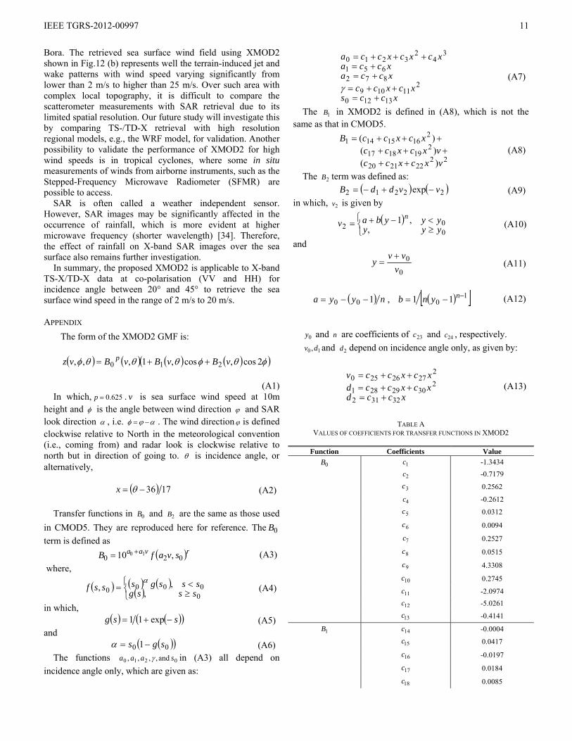
APPENDIX

The form of the XMOD2 GMF is:

2cos,cos,1,,, 210 vBvBvBvz p

(A1) In which, 625.0p . v is sea surface wind speed at 10m

height and is the angle between wind direction and SAR look direction , i.e. . The wind direction is defined clockwise relative to North in the meteorological convention (i.e., coming from) and radar look is clockwise relative to north but in direction of going to. is incidence angle, or alternatively,

1736 x (A2)

Transfer functions in 0B and 2B are the same as those used

in CMOD5. They are reproduced here for reference. The 0B

term is defined as

rvaa svafB 020 ,10 10 (A3) where,

00000 ,

,,sssgsssgsssf

(A4)

in which, ssg exp11 (A5)

and 00 1 sgs (A6)

The functions 0210 and,,,, saaa in (A3) all depend on

incidence angle only, which are given as:

xccsxcxcc

xccaxcca

xcxcxcca

13120

211109

872651

34

23210

(A7)

The 1B in XMOD2 is defined in (A8), which is not the same as that in CMOD5.

22222120

2191817

21615141

)( )( )(

vxcxccvxcxcc

xcxccB

(A8)

The 2B term was defined as:

22212 exp vvddB (A9) in which, 2v is given by

002 ,

,1yyyyyybav

n (A10)

and

0

0

v

vvy

(A11)

nyya 100 , 1

0 11 nynb (A12)

0y and n are coefficients of 23c and 24c , respectively.

10,dv and 2d depend on incidence angle only, as given by:

xccdxcxccdxcxccv

32312

23029281

22726250

(A13)

TABLE A

VALUES OF COEFFICIENTS FOR TRANSFER FUNCTIONS IN XMOD2

Function Coefficients Value

0B 1c -1.3434

2c -0.7179

3c 0.2562

4c -0.2612

5c 0.0312

6c 0.0094

7c 0.2527

8c 0.0515

9c 4.3308

10c 0.2745

11c -2.0974

12c -5.0261

13c -0.4141

1B 14c -0.0004

15c 0.0417

16c -0.0197

17c 0.0184

18c 0.0085

IEEE TGRS-2012-00997

12

19c -0.0145

20c -0.0009

21c -0.0004

22c 0.0011

2B 23c 7.4878

24c 0.8279

25c 19.6282

26c -14.6501

27c 14.4326

28c -0.0314

29c 0.1610

30c 0.1393

31c 0.6362

32c -0.0291

ACKNOWLEDGMENT

The TS-X/TD-X data were kindly provided by DLR via the AO proposals of OCE1044 and OCE1669. We acknowledge that buoy measurements were accessed from the NOAA/NDBC and Environment Canada networks, among which the data of buoy 48400 were provided kindly by Dr. Meghan Cronin at NOAA. We thank Dr. Thomas Bruns at DWD for providing the GSM model data. We especially thank Mr. Miguel Bruck for great help on ordering TS-X/TD-X data at buoy locations.

REFERENCES [1] A. Stoffelen, and D. Anderson, “Scatterometer data interpretation:

Estimation and validation of the transfer function CMOD4,” J. Geophys. Res., vol.102, no. C3, pp. 5767-5780, Mar.1997.

[2] Y. Quilfen, B. Chapron, T. Elfouhaily, K. Katsaros, and J. Tournadre, “Observation of tropical cyclones by high-resolution scatterometry,” J. Geophys. Res., vol.103, no.C4, pp.7767–7786, Apr.1998.

[3] H. Hersbach, A. Stoffelen and S. de Haan, “An Improved C-band scatterometer ocean geophysical model function: CMOD5”, J. Geophys. Res., 2007, vol.112, C03006, Mar.2007, doi:10.1029/2006JC003743.

[4] H. Hersbach, “CMOD5.N: A C-band geophysical model function for equivalent neutral wind,” ECMWF Tech. Memo. 554, ECMWF, Reading, U. K, 2008.

[5] A. Stoffelen, and D. Anderson, “Scatterometer Data Interpretation: Measurement Space and Inversion.” J. Atmos. Oceanic Technol., vol.14, no.6, pp.1298–1313, Dec.1997.

[6] S. Lehner, J. Horstmann, W. Koch, and W. Rosenthal, “Mesoscale wind measurements using recalibrated ERS SAR images”, J. Geophys. Res., vol.103, no. C4, pp. 7847–7856, Apr. 1998.

[7] X.-F. Li, W. Zheng, W.G. Pichel, C.-Z. Zou, and P.C. Clemente-Colon, “Coastal katabatic winds imaged by SAR”, Geophys Res. Lett., 34: L03804, doi:10.1029/2006GL028055, Feb. 2007.

[8] R. P. Signell, J. Chiggiato, J. Horstmann, J. Pullen, and F. Askari, “High-resolution mapping of Bora winds in the northern Adriatic sea using synthetic aperture radar” J. Geophys. Res, vol. 115, C04020, doi: 1029/2009JC005524, Apr.2010.

[9] X.-M. Li, X.-F. Li, and M.-X. HE, “Coastal upwelling observed by multi-satellite sensors,” Sci. China Ser. D-Earth Sci., vol. 52, no.7, pp. 1030-1038, doi: 10.1007/s11430-009-0088-x, Jul.2009.

[10] M. B. Christiansen and C. B. Hasager, “Wake effects of large offshore wind farms identified from satellite SAR”, Remote Sens. Environ., vol.98, no. 2–3, pp.251-268, Oct. 2005.

[11] D. R. Thompson, T.M. Elfouhaily, and B. Chapron, “Polarisation ratio for microwave backscattering from the ocean surface at low to moderate incidence angles”, Geoscience and Remote Sensing Symposium Proceedings, 1998, vol.3, pp.1671-1673, Jul. 1998.

[12] A. A. Mouche, D. Hauser, J.-F. Daloze, C. Guerin, “Dual-polarisation measurements at C-band over the ocean: results from airborne radar observations and comparison with ENVISAT ASAR data”, IEEE Trans. Geosci. Remote Sens., vol.43, no.4, pp. 753- 769, Apr. 2005.

[13] T. Elfouhaily, “Physical modeling of electromagnetic backscatter from the ocean surface; Application to retrieval of wind fields and wind stress by remote sensing of the marine atmospheric boundary layer, Ph.D. diss., Univ. Paris VII, Paris, France, 1996.

[14] J. Horstmann, W. Koch, S. Lehner, and R. Tonboe, “Wind retrieval over the ocean using synthetic aperture radar with C‐band HH polarisation”, IEEE Trans. Geosci. Remote Sens., vol.38, no. 5, pp. 2122–2131, doi:10.1109/36.868871, Sep.2000.

[15] Vachon, P. W., and F. Dobson, “Wind retrieval from RADDARSAT SAR images: Selection of a suitable C‐band HH polarisation wind retrieval model”, Can. J. Rem. Sens., vol. 26, pp. 306–313, Jan.2000.

[16] F. M. Monaldo, D. R. Thompson, W. G. Pichel, and P. Clemente‐Colon, “Comparison of SAR‐derived wind speed with model predictions and ocean buoy measurements”, IEEE Trans. Geosci. Remote Sens., vol.39, no.12, pp.2587–2600, doi:10.1109/36.974994, Dec.2001.

[17] B. Zhang, W. Perrie, and Y. He, “Wind speed retrieval from RADARSAT-2 quad-polarisation images using a new polarisation ratio model”, J. Geophys. Res., 116, C08008, doi:10.1029/2010JC006522, Aug.2011.

[18] O. Isoguchi and M. Shimada, “An L-band ocean geophysical model function derived from PALSAR,” IEEE Trans. Geosci. Remote Sens., vol. 47, no. 7, pp. 1925–1936, Jul. 2009.

[19] Y.-Z. Ren, S. Lehner, S. Brusch, X.-M. Li, and M.-X. He, “An algorithm for the retrieval of sea surface wind fields using X-band TerraSAR-X data”, Int. J. Remote Sens., vol.33, no.23, pp. 7310–7336, Dec.2012.

[20] W.-Z. Shao, X.-M. Li, S. Lehner, C.-L. Guan, “Development of polarisation model for TerraSAR-X to retrieve sea surface wind field”, Int. J. Remote Sens., in revision, 2013.

[21] D.R. Thompson, J. Horstmann, A. Mouche, N. S. Winstead, R. Sterner, and F. M. Monaldo, “Comparison of high-resolution wind fields extracted from TerraSAR-X SAR imagery with predictions from the WRF mesoscale model”, J. Geophys. Res., vol. 117, C02035, doi:10.1029/2011JC007526, Feb.2012.

[22] M. Schwerdt, B. Brautigam, M. Bachmann, B. Doring, D. Schrank, and J. Hueso Gonzalez, “Final TerraSAR-X calibration results based on novel efficient methods,” IEEE Trans. Geosci. Remote Sens., vol. 48, no. 2, pp. 677–689, Feb. 2010.

[23] M. Schwerdt, D. Schrank, M. Bachmann, J. H. Gonzalez, B. J. Doring, T.-R. Nuria, and A. J. Walter, “Calibration of the TerraSAR-X and the TanDEM-X satellite for the TerraSAR-X mission”, 9th European Conference on Synthetic Aperture Radar, EUSAR, pp.56-59, 23-26 April 2012.

[24] M. Eineder, T. Fritz, J.Mittermayer, A. Roth, E. Borner, and H. Breit, “Terrasar-x ground segment. basic product specification document.” DLR, TX-GS-DD-3302, issue 1.7, 2010.

[25] J. P. Peixoto, and A. H. Oort, “Physics of Climate”, Am. Inst. of Phys., Woodbury, N.Y., 1992.

[26] W. T. Liu, and W. Tang, “Equivalent neutral wind”, JPL Publ., 96-17, Jet Propul. Lab., Pasadena, Calif., 1996.

[27] C. A. Mears, D. K. Smith, and F. J. Wentz, “Comparison of Special Sensor Microwave Imager and buoy-measured wind speeds from 1987 to 1997”, J. Geophys. Res., 106(C6), pp. 2156 – 2202, doi: 10.1029/1999JC000097, June 2001.

[28] D. B. Chelton and M. H. Freilich, “Scatterometer-based assessment of 10-m wind analyses from the operational ECMWF and NCEP numerical weather prediction models,” Mon. Weather Rev., vol. 133, no. 2, pp. 409–429, Feb. 2005.

[29] A. H. Monahan, “The probability distribution of sea surface wind speeds. Part I: Theory and SeaWinds observations”, J. Climate, vol.19, pp. 497–520, Feb.2006.

[30] M. Portabella and A. Stoffelen, “On scatterometer ocean stress,” J. Atmos. Ocean. Technol., vol. 26, no. 2, pp. 368–382, Feb. 2009.

[31] F. J. Wentz and D. K. Smith, “A model function for the ocean normalized cross section at 14 GHz derived from NSCAT observations”, J. Geophys. Res., vol.104, no.c5, pp. 11499–11514, May 1999.

[32] T.-Y. Koh, S. Wang, B. C. Bhatt, “A diagnostic suite to assess NWP performance”, J. Geophys. Res., vol. 117 (D13), Jul. 2012.

[33] H. Masuko, K. Okamoto , M. Shimada and S. Niwa, “Measurement of microwave backscattering signatures of the ocean surface using X band and Ka band airborne scatterometers”, J. Geophys. Res., vol. 91, no. c11, pp.13605 -13083, Nov.1986.

IEEE TGRS-2012-00997

13

[34] C. Melsheimer, W. Alpers, and M. Gade, “Investigation of multifrequency/multipolarisation radar signatures of rain cells over the ocean using SIR-C/X-SAR data,” J. Geophys. Res., vol. 103, pp.18 851–18 866, Aug. 1998.

Xiao-Ming Li received the B.S. degree in electronic and information engineering from Xi’an Communication College, People’s Liberation Army, Xi’an, China, in 2002, the (equivalent) M.S. degree, with work focusing on satellite ocean remote sensing, from the Ocean University of China, Qingdao, China, in 2006, and the Ph.D. degree in geophysics from the

University of Hamburg, Hamburg, Germany, in 2010. Since 2006, he has been with the Remote Sensing Technology Institute, German Aerospace Center (DLR), Wessling, Germany. His research interests include synthetic aperture radar ocean wave algorithm development, investigation of extremely oceanic weather, and observation of ocean dynamics using spaceborne multisensors.

Susanne Lehner (M’01) received the M.Sc. degree in applied mathematics from Brunel University, Uxbridge, U.K., in 1979 and the Ph.D. degree in geophysics from the University of Hamburg, Hamburg, Germany, in 1984. She was a Research Scientist with Max-Planck Institute for Meteorology, Hamburg. In 1996, she joined the German

Remote Sensing Data Center, German Aerospace Center (DLR), Wessling, Germany. She is currently the Head of the SAR oceanography team with the Remote Sensing Technology Institute, DLR, working on the development of algorithms determining marine parameters from synthetic aperture radar.