The 183-WSL fast rain rate retrieval algorithm. Part I: Retrieval design

Sante Laviola *, and Vincenzo Levizzani

ISAC-CNR, Bologna, Italy

*Corresponding author: ISAC-CNR, via Gobetti 101, I-40129 Bologna, Italy. Tel: +39-051-6398019. Fax: +39-051-6399658. E-mail address: s.laviola@isac.cnr.it.

Manuscript submitted to Atmospheric Research

ARTICLE

1

ABSTRACT

The Water vapour Strong Lines at 183 GHz (183-WSL) fast retrieval method retrieves rain

rates and classifies precipitation types for applications in nowcasting and weather monitoring.

The retrieval scheme consists of two fast algorithms, over land and over ocean, that use the water

vapour absorption lines at 183.31 GHz corresponding to the channels 3 (183.31±1 GHz), 4

(183.31±3 GHz) and 5 (183.31±7 GHz) of the Advanced Microwave Sounding Unit module B

(AMSU-B) and of the Microwave Humidity Sounder (MHS) flying on NOAA-15-18 and Metop-

A satellite series, respectively.

The method retrieves rain rates by exploiting the extinction of radiation due to rain drops

following four subsequent steps. After ingesting the satellite data stream, the window channels at

89 and 150 GHz are used to compute scattering-based thresholds and the 183-WSLW module for

rainfall area discrimination and precipitation type classification as stratiform or convective on the

basis of the thresholds calculated for land/mixed and sea surfaces. The thresholds are based on

the brightness temperature difference Δwin = TB89 – TB150 and are different over land (L) and over

sea (S): cloud droplets and water vapour (Δwin < 3 K L; Δwin < 0 K S), stratiform rain (3 K < Δwin

< 10 K L; 0 K < Δwin < 10 K S), and convective rain (> 10 K L and S). The thresholds, initially

empirically derived from observations, are corroborated by the simulations of the RTTOV

radiative transfer model applied to 20000 ECMWF atmospheric profiles at midlatitudes and the

use of data from the Nimrod radar network. A snow cover mask and a digital elevation model are

used to eliminate false rain area attribution, especially over elevated terrain. A probability of

detection logistic function is also applied in the transition region from no-rain to rain adjacent to

the clouds to avoid ensure continuity of the rainfall field. Finally, the last step is dedicated to the

2

rain rate retrieval with the modules 183-WSLS (stratiform) and 183WSLC (convective), and the

module 183-WSL for total rainfall intensity derivation.

A comparison with rainfall retrievals from the Goddard Profiling (GPROF) TRMM 2A12

algorithm is done with good results on a stratiform and a hurricane case studies. A comparison is

also conducted with the MSG-based Precipitation Index (PI) and the Scattering Index (SI) for a

convective-stratiform event showing good agreement with the 183-WSLC retrieval. A complete

validation of the product is the subject of Part II of the paper.

Keywords: Hydrology, meteorology, microwave radiometry, precipitation, rain rate, remote

sensing, weather satellite.

3

1. Introduction and physical basis

The increased sensitivity of the last generation of passive microwave (PMW) sensors has

considerably enhanced the capabilities of atmospheric sounding from satellite with an

unprecedented level of accuracy. Microwave radiometry for space observations over the last

decade has developed along two parallel pathways: a) increase of the radiometers’ spatial

resolution with new opportunities for observing small scale events, and b) expansion of the

frequency range to higher frequencies with increased sensitivity to small size hydrometeors.

AMSU-B is the high frequency and high spatial resolution module of the Advanced

Microwave Sounding Unit (AMSU). It is a cross-track scanning instrument covering the

sounding angles ± 48.5° with a nominal field of view of 1.1° (≈ 15 km at nadir) (Saunders et al.,

1995). Its five-channels range from 90 to 190 GHz; the first two channels, the so-called window

channels, are centred on two atmospheric windows at 89 and 150 GHz, respectively, particularly

employed for surface emissivity studies (e.g., Felde and Pickle, 1995) and cloud ice particle

detection.

The absorption frequencies at 183.31 GHz are located in a strong water vapour absorption

band (e.g., Chen, 2004; Leslie and Staelin, 2004). They have been generally employed to retrieve

the amount of total precipitable water or the water vapour profiles (Rosenkranz, 2001) also in dry

or very dry atmospheric conditions (Staelin et al., 1976).

1.1. The window channels at 89 and 150 GHz

The absorption and scattering properties of the atmospheric water column are governed by

particle phase, size distribution, aggregate density, shape, and dielectric constant (e.g., Bauer et

4

al., 2005; Bennartz and Petty, 2001; Kummerow and Weinman, 1988; Mugnai et al., 1993; Petty,

2001; Skofronick-Jackson et al., 2002; Wilheit et al., 1982; Wu and Weinman, 1984).

The window channel at 89 GHz can be considered as the PMW analog to the 11 µm

channel in the thermal infrared (IR) (Muller et al., 1994). The main difference is that PMW

channels can partially penetrate clouds thus being very sensitive to the cloud microphysical

composition. Over an ocean background the window channels contribute information on

precipitation via their sensitivity to the warm emission signature of precipitating clouds and their

sensitivity to scattering. Algorithms were first designed based on AMSU window channels

(Grody et al., 2000; Weng et al., 2003) with quality comparable to that of the products that make

use of conical scanners such the Special Sensor Microwave/Imager (SSM/I) and with the high

resolution typical of the AMSU sensor.

The idea of using high frequencies to retrieve rainrates was to dwell on the scattering from

ice hydrometeors, which is applicable over land as well as over ocean (Grody et al., 2000). The

brightness temperature (TB) depression at 150 GHz is a measure of the scattering of ice particles

growing to precipitation size and thus provides an opportunity for an indirect measurement of

precipitation. As noted by several authors (Bennartz and Bauer, 2003; Chen and Staelin, 2003;

Ferraro et al., 2000), the 150 GHz channel is sensitive to smaller size particles with respect to the

89 GHz channel and also provides a more physical link with the density and size of ice particles

associated with precipitation. Ice crystal shape has also a significant influence (Evans and

Stephens, 1995a, b). Their use thus improves precipitation area delineation and contributes to a

better quantification of stratiform rain. Scattering index (SI) approaches are adopted to estimate

the probability associated to the surface rain intensities (Bennartz et al., 2002; Ferraro et al.,

2005; Grody et al., 2000). SI methods dwell on the values of the TB difference at window

5

frequencies (Δwin = TB89 - TB150) to define precipitation intensity classes and classify surface rain

into a number of categories via a calibration with ground data. For example, a simultaneous

derivation of the cloud ice water path (IWP) and ice particle effective diameters is conducted

from the AMSU channels at 89 and 150 GHz (Zhao and Weng, 2002; Ferraro et al., 2005); the

IWP is then converted into the surface rain rates through an IWP - rainfall rate relationship

developed from cloud model results (Weng et al., 2003).

1.2. The 183.31 GHz AMSU-B channels

The other three AMSU-B channels were selected within the strong water vapour absorption

band at 183.31 GHz. They are centred at 183±1, 183±3 and 183±7 GHz and commonly defined

as the 184, 186 and 190 GHz channels. Along the same line of thought mentioned for

introducing the 89 GHz-11 µm analogy, the 183 GHz channels can be thought as the PMW

analogs of the IR 6.3 µm water vapour band. In fact, they were originally designed and dedicated

to the profiling of the atmospheric water vapour (Kakar, 1983; Lambrigtsen and Kakar, 1985;

Wang and Chang, 1990; Wilheit, 1990) or to the retrieval of the total precipitable water (Wang

and Wilheit, 1989). However, several studies have demonstrated the sensitivity of these channels

to rain drops and ice crystals (Bennartz and Bauer, 2003; Burns et al., 1997; Greenwald and

Christopher, 2002; Isaacs and Deblonde, 1987; Surussavadee and Staelin, 2006). The water

vapour absorption lines at these wavelengths ideally complement the window channels for clouds

and precipitation observations (Deeter and Vivekanandan, 2005; English, 1995; English et al.,

1994; Leslie and Staelin, 2004; Racette et al., 1996) and modelling (DiMichele and Bauer, 2006;

Hong et al., 2005).

6

Due to their weighting functions peaking between 2 and 8 km altitude, low-level clouds

have little effect on the signal in the moisture channels around 183.31 GHz. On the other hand,

cloud formations higher than 2 km largely contribute to the radiation extinction because of the

combination of absorption by large rain drops and scattering by ice crystals. The magnitude of

the signal extinction depends both on the height of the scattering hydrometeors and on the

channel wavelength: cold and thick clouds mostly depress the signal at frequencies farther from

the centre of the band with respect to the closer ones. Additionally, all these channels, including

the one at 150 GHz, are influenced by ice particles in thick cirrus clouds (Buehler et al., 2007;

Hong et al., 2005).

Of interest for precipitation estimation is the influence of liquid and ice cloud hydrometeors

on upwelling radiation at these wavelengths: water drops attenuate upwelling radiances by

absorbing and re-emitting radiation while ice crystals depress the incoming signal through

multiple scattering. The latter effect can be observed in Fig. 1, which refers to convective cells

rapidly forming during an intense storm over northern Italy on 1 June 2007. Note that large ice

aggregates, typically > 20 µm, appear to scatter radiation at 190 GHz (Fig. 1c) located at the

wings of the absorption band where scattering by ice crystals is less masked by the water vapour

aloft with respect to the other two frequencies. Sensitivity studies for deep convection show that

the water vapour surrounding or inside the cloud significantly absorbs the incident radiation at

190 GHz (influence is to be detected also on the window channels) above 5 km (Hong et al.,

2005) sometimes attenuating the scattering due to the ice hydrometeors beneath; below 5 km the

sensitivity is much less or virtually non-existent. It was found that the  sensitivity  to  graupels  at  

all   channels   is   stronger   than   that   to   cloud   ice   and   snow   (Hong et al., 2005);   the  190  GHz  

channel  has  a  stronger  sensitivity  than  the  other  channels  to  frozen  hydrometeors.    At  the  

7

channels   closer   to   the  water  vapour  absorption   line,   the   sensitivity   is   strongest   to   frozen  

hydrometeors  at  high  altitudes.    The  TBs  at  the  three  water  vapour  absorption  channels  are  

mainly   sensitive   to   frozen   hydrometeors   above   7   km.     The   183.3   ±   1   GHz   channel   has  

virtually  no  sensitivity  to  frozen  hydrometeors  below  7  km.    The  TB  difference  between  the  

184  GHz  channel  and  the  190  GHz  channel  is  generally  sensitive  to  liquid  water  above  5  km  

and   frozen   hydrometeors   above   7   km.     While   moving towards the central peak of the

absorption band a very small scattering signature can be observed except when intense updrafts

drag frozen aggregates up to the top of the troposphere as in Fig 1a.

The opacity of atmosphere at the three absorption channels around 183.31 GHz

significantly masks variations due to changes of surface emissivity thus paving the way to

successful soundings over any surfaces. Only in very dry atmospheric conditions and in presence

of low temperature profiles these frequencies start sensing surface effects. An example of this

fact stems out by examining Fig. 2 where the scattering of snow over the Alps at 184-190 GHz

during the month of February 2004 is shown. Note that the TB depression in Fig. 2c, due to the

snow over the Alps and the Balkans, is quite similar to a scattering signal by frozen hydrometeors

as is the case of the structure in the centre of Fig. 2b and 2c.

However, since the peaks of the weighting functions vary from 2 to 8 km, the advantage of

sounding in any emissivity condition could rather reveal a disadvantage while observing shallow

precipitation forming within lower atmospheric layers, which cannot be sensed altogether.

Modifications of cloud emission temperatures and liquid water content affect all opaque

frequencies according to their weighting function distributions. Therefore, the 190 GHz

frequency, whose weighting function peaks closer to the surface, is more affected by low level

clouds (around 2 km) than by higher level clouds. On the other hand, the central band frequency

8

at 184 GHz becomes significantly sensitive to the cloud bulk above 6 km. Low level liquid

clouds are completely transparent to this frequency.

In the case of ice clouds (hailstones, snowflakes) the scattering by ice hydrometeors

extinguishes radiation two to three orders of magnitude more than in the case of pure emission.

This is observed in Fig. 1c where a TB depression due to ice aggregates close to 70 K is measured

at 190 GHz.

The 183.31 GHz spectral band can thus be clearly identified as a powerful tool for the

observation of precipitation regimes formed in warm rain, mixed phase and ice cloud conditions.

1.3. Scattering- and emission-based PMW precipitation estimation algorithms

Scattering and emission properties of precipitation in the microwaves were first identified

at the end of the 70s by means of the Electrically Scanning Microwave Radiometer (EMSR; see

for example Barrett and Martin, 1981; Weinman and Guetter, 1977; Wilheit et al., 1977) on board

Nimbus 5 and 6. Starting soon after, algorithms were proposed based on an increasing number of

microwave spectral channels that helped identifying clouds and precipitation features over the sea

(e.g., Wilheit et al., 1982) and over land (e.g., Spencer, 1984). A range of algorithms based on a

variety of different approaches were subsequently developed. The following algorithm

categories can be roughly separated: polarization corrected temperature thresholds (PCT; Spencer

et al., 1989; Kidd, 1998), radiative transfer and columnar model retrievals (Aonashi et al., 1996;

Bauer, 2001; Bauer et al., 2001; Liu and Curry, 1992; Wentz, 1997), statistical-physical retrievals

(Kummerow and Giglio, 1994a, b; Kummerow et al., 2001; Mugnai et al., 1993; Olson, 1989;

Petty, 1994a, b; Smith et al., 1992; Surussavadee and Staelin, 2008a, b), Bayesian retrievals

(Evans et al., 1995; Kummerow et al., 1996), thresholding and scattering/emission-based

9

retrievals (Ferraro, 1997; Ferraro and Marks, 1995; Ferraro et al., 2005; Kongoli et al., 2007;

McCollum and Ferraro, 2003; Prabhakara et al., 1999; Prabhakara et al., 2000; Weng et al.,

2003), neural network-based retrievals (Staelin and Chen, 2000). For a general overview of

satellite rainfall estimation methods, including PMW methods, the reader is referred to recent

books and reviews (Levizzani et al., 2007; Kidd et al., 2009a, b; Michaelides et al., 2009).

In particular, several approaches to precipitation estimation using both window and opaque

channels onboard AMSU-A and B were adopted in the recent past. Global operational

algorithms that make use of absorption channels for the operational production of rainfall maps

are the Microwave Surface and Precipitation Products System (MSPPS) (Ferraro et al., 2005) of

the National Oceanic and Atmospheric Administration (NOAA), and the Global Satellite

Mapping of Precipitation (GSMaP) Project (Aonashi et al., 2009; Kubota et al., 2007) for which

an over-ocean retrieval algorithm for PMW sounders was conceived (Shige et al., 2009). A

global algorithm was conceived by Staelin and Chen (2000) using a neural network and a

NEXRAD radar database and successively expanded to use more channels (Chen and Staelin,

2003); the algorithm was successively modified using a cloud-resolving numerical weather

prediction model to produce the training database (Surussavadee and Staelin, 2007, 2008a, b).

Note that the success of any PMW rain retrieval algorithm critically depends on the

rain/no-rain screening methodology (e.g., Ferraro et al., 1998; Kida et al., 2009; Seto et al., 2005,

2008), which is unavoidable over land where also surface type classification is crucial (e.g.,

Basist et al., 1998; Grody, 1991; Neale et al., 1990).

10

1.4. Structure of the paper

A fast PMW algorithm, the Water vapour Strong Lines at 183 GHZ (183-WSL), is

proposed for the estimation of rainfall rates on the basis of measurements in the resonant water

vapour band at 183.31 GHz of the AMSU-B sensor flying on board the NOAA spacecrafts series.

The physical approach of the 183-WSL algorithm is mainly based on the absorption-emission

processes of radiation at 183.31 GHz, as already preliminarily introduced by Laviola and

Levizzani (2008, 2009) and based on previous studies by Laviola (2006a, b). The retrieval

method differs from that of the other algorithms in that it is entirely based on window and

absorption frequencies of the cross track sounders. The product has thus the highest spatial

resolution among the PMW-based ones and is suited for operational applications using the

constellation of NOAA and Metop satellites.

In the following section the description of the algorithm and its modules will be given. In

section III retrieval examples will be discussed together with a comparison with the Goddard

Profiling algorithm (GPROF) (Kummerow et al., 2001) and the MSG-based Precipitation Index

(MSG-PI, Thoss et al., 2001) and the Scattering Index (SI, Bennartz et al., 2002) for three case

studies: stratiform, midlatitudes mixed type, and tropical cyclonic. A discussion of these first

results will be provided in section IV.

2. The 183-WSL Algorithm

In Fig. 3 a flow chart of the 183-WSL algorithm is shown in its present working

configuration. In the following a detailed description of the steps 1-4 of the algorithm and of the

various modules is provided. Note that the present version of the algorithm is designed to work

11

only on liquid precipitation while the snowfall detection and estimation is in advanced study

state. However, this latter will be discussed in future papers.

The first step is dedicated to ingesting and processing the satellite data stream. All relevant

information, namely TBs, surface type (land/sea/mixed), satellite local zenith angles, and

topography, are separated from the data stream and arranged for input into the 183-WSL

processing chain. Pixel data are limb-corrected according to the sensor scanning geometry. The

second step consists of land/sea/other pixel detection that classifies all sounded pixels; at this

stage a water vapour and snow cover filter is also applied. The third step is dedicated to the

estimation of the convective and stratiform components of rainfall and the last step computes the

total rainrates as a sum of the convective and stratiform intensities.

2.1. Window frequencies: rain/no-rain identification and convective-stratiform rain

classification

A sensitivity study on the behaviour of the 89 and 150 GHz AMSU-B channels in clear-sky

and rainy conditions was conducted by Laviola (2006b) using a synthetic dataset. The dataset

was generated using RTTOVSCATT (Burlaud et al., 2007; O’Keeffe et al., 2004), a version of

the radiative transfer model RTTOV (Eyre, 1991; Matricardi et al., 2004; Saunders et al., 2009)

that handles the scattering of radiation by hydrometeors through the delta-Eddington

approximation (Kummerow, 1993; Wu and Weinman, 1984). The Eddington approach to

scattering approximates the radiance vector and the phase function to the first order so that only

one angle is required for the scattering calculations. The Marshall-Palmer size distribution

(Marshall and Palmer, 1948) function for rain droplets and a modified gamma for ice crystals

(Evans and Stephens, 1995a, b) are assumed. RTTOVSCAT was applied to 20000 atmospheric

12

profiles in clear and rainy conditions from the model of the European Centre for Medium-Range

Weather Forecasts (ECMWF).

As  an  example,  Figure  4  shows  the  scatter  plots  of  the  89  and  150  GHz  synthetic  data  

of   rainy   versus   clear   sky   conditions   over   the   ocean   (note   that   a   subset   of   9500   ECMWF  

atmospheric   profiles   was   used);   the   “rainy”   profiles   refer   to   atmospheric   columns  

containing  cloud  droplets,  cloud  ice,  and  liquid  and  solid  precipitation  hydrometeors.    The  

atmospheric   columns   associated   with   rainy   conditions   significantly   absorb   the   89   GHz  

radiation  increasing  the  TBs  of  about  40  K  with  respect  to  the  clear  sky  conditions.    At  150  

GHz  the  scattering  from  precipitation  hydrometeors  depresses  the  TBs  of  about  30  K.  

The radiation at 89 GHz is markedly extinguished by increasing water content. Cloud

liquid water or low-layered clouds absorb the upwelling radiation generally increasing the

outgoing signal when the surface emissivity ε is low (Bennartz et al., 2002). On warmer surfaces

(ε > 0.90) the opposite situation will usually be observed. In a very humid atmosphere the 150

GHz frequency behaves more like a “low-level” water vapour channel than as a window channel

with its weighting function peaking higher up around 850 hPa (Bennartz and Bauer, 2003). In

the case of drier profiles the channel goes back to its quasi-transparency.

These facts suggest a way to exploit the effects of cloud liquid water amount variations and

cloud positioning in the frequency range 89-150 GHz (Bennartz and Bauer, 2003; Muller et al.,

1994). Liquid water clouds, corresponding to low rain rate intensities, generally tend to suppress

the effect of surface emissivity, particularly at 89 GHz, whereas higher clouds influence more the

150 GHz signal (Laviola, 2006a). For example, a 1 km-thick cloud located at 2-3 km over land

absorbs radiation near 89 GHz resulting in a slight decrease of TBs while it attenuates the signal

down by ≈ 60 K more in the case of colder clouds at 10 km height. At 150 GHz low clouds

13

impact a few K less than the nominal (clear sky) channel value and the extinction by colder

clouds depresses the signal drastically more than 30 K in dependence of cloud altitude.

It is thus conceivable that, by appropriately combining the radiometric features of the 89

and 150 GHz channels, precipitating areas can be delineated both over land and over water

surfaces on the basis of absorption and scattering induced by different hydrometeor states. An

example is given in Fig. 5d where the Δwin = TB89 – TB150 is shown in occasion of a Saharan dust

transport towards Greece, the Balkans and reaching Bulgaria. The dust plume is spotted by the

Meteosat Second Generation (MSG) Spinning Enhanced Visible and InfraRed Imager (SEVIRI)

(Schmetz et al., 2002); the multispectral image (MSG day microphysical; Kerkmann et al., 2006;

Rosenfeld and Lensky, 1998) in Fig. 5a shows the plume as pale yellow. The bright orange area

are clouds tops characterized by small ice crystals, probably due to strong updrafts. Much larger

ice crystals are detected over Italy (red). In the occasion, a “red rain” phenomenon was

registered over Bulgaria. Only optically thick clouds contrast with the cold background with a TB

> 0 K. The reasons can be found in the microphysics of the observed clouds. The cloud system

over the Black Sea is located into the first atmospheric layers and mostly formed by liquid drops

thus absorbing more at 89 GHz than scattering at 150 GHz. On the contrary, in correspondence

of the deep convection over Central Italy scattering by ice particles is more pronounced at 150

GHz than the absorption at 89 GHz. In both cases the net balance results is an increase of the

Δwin values. The presence of ice aggregates aloft, evidenced at 150 GHz where the signal is

attenuated by about 50 K, is less evident at 89 GHz with respect to other low-scattering clouds.

This is due to the presence of a layer of saturated water vapour above the clouds, which screens

the radiation scattered by ice. Conversely, the absorbing liquid water large drops are well

detected.

14

The SI approach (Bennartz et al., 2002) and the successive modification by Laviola (2006a,

b) is the basis of the 183-WSLW (the final W standing for water vapour) screening module,

which discriminates between rainy and non-rainy clouds on the basis of a rainfall dataset at 5 km

resolution of the UK MetOffice Nimrod radar network (http://badc.nerc.ac.uk/data/nimrod/). The

thresholds are reported in Table 1. It is found that over land, when Δwin < 3 K the observed pixels

are classified as non rainy and therefore removed from the computation. Over open water, where

the impact of the atmospheric parameters is greater than over land, the previous threshold is

reduced to 0 K. An example of the effects of applying the 183-WSLW module is visible in Fig. 6

where a generalized false attribution of low rainrates is done by the algorithm when the rain/no-

rain screening is not adopted. Note that all false rainfall signatures are associated with

substantially low rain intensity values as it is to be expected.

The SI approach based on Δwin is also applied to differentiate between convective and

stratiform rain types. The strong scattering by growing ice hydrometeors, which typically

characterize convective cell formations, induces a clear signature at 150 GHz depressing the

TB150 of several K with respect to what happens to TB89. These different sensitivities to the

presence of ice has been exploited to calculate a fixed threshold value based on the Nimrod radar

database. Generally, Δwin < 10 K values are associated with stratiform precipitation whereas

values higher than these can be correlated to the more scattering convective cells. Table 1 details

the various empirical thresholds over land and sea for the two categories. Fig. 5e and 5f report

the performance of the modules 183-WSLC (convective) and 183-WSLS (stratiform),

respectively. Additional evidence is provided for a stratiform and a mixed/convective system in

Section 3.1 and 3.2, respectively.

15

Note that, due to the presence of ice into the cloud cores, just the borders of precipitating

clouds are “warmer” and thus recognized as stratiform rain. In fact, in these areas the

coexistence of large amount of droplets, typically of a few microns size, with drops associated

with light-rain stratiform clouds of comparable dimensions is crucial to distinguishing rain from

no-rain pixels. Moreover, being the estimation of rainfall based on the 183.31 GHz frequencies

(see next sub-section), which sense the water vapour distribution variations, the strong absorption

by water vapour molecules could reveal indistinguishable from the absorption due to raindrops,

thus inducing strong overestimations.

In addition, tests carried out during the winter reveal that the scattering signal at 190 GHz

relative to the snow cover on mountain tops is analogous to the ice signature on convective cloud

tops. Therefore, a snow threshold as a combination of Δwin values over land and topographic

information from a digital elevation model (DEM) is applied to further remove false rain signals

from the 183-WSL estimations.

The derived thresholds may not be valid for climate regions characterized by low

temperature profiles and possible frozen soil. At very high latitudes, for example, the sounding at

89 and 150 GHz is strongly influenced by the high variability of surface emissivity except for the

open waters scenario (Mathew et al., 2006; Todini et al., 2009).

The Microwave Humidity Sounder (MHS) onboard the Metop series has slightly different

channels at 89 and 157 GHz, thus different from those of AMSU-B. Sensitivity tests have shown

that the rain/no-rain screening of the 183-WSL method does not show appreciable differences

when using these other channels. The water vapour absorption at lower levels would tend to

increase, but this does not show differences in the performances of the algorithm.

16

2.2. Rainrate estimation

The fast algorithm 183-WSL is based on a linear combination of the AMSU-B opaque

channels at 183.31 GHz and is the result of a multiple linear regression between the TBs of the

183.31 GHz channels of the AMSU-B radiometer and the radar-derived rainfall rates of the

Nimrod network (Laviola, 2006a, b). A data convolution was necessary to match the different

resolution of the radar data (5 km) and that of AMSU-B (15 km at nadir). The effect of limb

darkening of the instrument has been considered through the use of the cosine of the zenith angle.

Rain rates are retrieved in mm h-1 both over land and sea by sounding cloud features from

1-2 km up to the top of the troposphere according to the channel weighting function.

Rain rate values between 0.1 and 20 mm h-1, representing the 183-WSL sensitivity to

different rain types, are employed to infer the precipitation amount for the latitude range ± 60

degrees. However, further investigations have demonstrated a possible variation of the threshold

values when the 183-WSL is applied over regions where atmospheric conditions such as

temperature lapse rate and humidity profiles are extremely variable, e.g. over tropical areas where

rain rates up to 30 mm h---111 are observed. On the other hand, over regions located at latitudes

above 60 degrees, characterized by low temperatures especially closer to the surface, when the

latitude becomes > 70 degrees, the estimation of rainfall intensities < 2 mm h-1 becomes crucial.

The land algorithm is as follows

( ) 186184190 BBBl CTTTBARR +−×+= (1)

where A= 19.12475, B= -0.206044 and C= -0.0565935 are coefficients of the multiple regression

analysis. The following adjustment is used to improve estimations with equation (1):

17

6972.0−= ll RRRR (2)

The sea algorithm has the following form

( ) 186184190 BBBs FTTTEDRR +−×+= (3)

where D= 9.6653, E= -0.3826 and F= -0.01316 are coefficients of the multiple regression

analysis. Again, two adjustments are applied to improve the algorithm in 3:

( ) 3510.15.04 −×+= ss RRRR (4)

Equations (2) and (4) represent an adjustment of the first calibration of the retrieval

algorithm derived using an independent radar dataset over the same area of the initial calibration.

2.3. Application of a Probability Of Rain Detection Function (PORDF)

A further improvement for a better delineation of the rain areas is introduced. The basic

concept is that more pixels associated with high values of condensed water vapour, particularly

during light rain events, can be associated with clouds in a growing stage depending on their

water vapour amount. With increasing drop size the freshly nucleated droplets can develop into

light stratiform rain. To describe this process a Probability Of Rain Development Function

(PORDF) has been conceived.

18

The PORDF stems from the concept of an evolutional logistic model (Hilbe, 2009) where

the starting element of the population are pixels associated with rain rate values > 2 mm h-1, as

shown in Fig. 7. The coefficients of the PORDF model were previously calculated using an ad

hoc model, which links rain clouds observed in the IR (200 < TB < 253 K) and the 183-WSLW-

retrieved values (Fig. 8).

The PORDF is activated when discarded pixels, classified as cloud droplets (i.e., non

rainy), correspond to rain rates > 2 mm h-1. This limit value is considered as a crucial threshold

between cloud droplets (non precipitating) and the beginning of stratiform rain development

(light precipitation). The 2 mm h-1 threshold is considered valid at mid-latitude and tropics (e.g.,

Adler and Negri, 1988). At higher latitudes (> 50°), characterized by light or very-light rainfall

(often < 2-3 mm h-1), the use of PORDF can induce underestimations.

The effects of the application of the PORDF on the 183-WSL rainfall retrievals are

documented for two events: 18 January 2007 and 23-24 March 2008 (Fig. 9). Note the

discontinuity of the rainfall field in the areas of low rainrates due to obvious underestimation

where the 183-WSLW module discards cloud areas deemed non-precipitating, but that are in

reality characterized by low rain intensities. The overall result is visually appreciated as a better

continuity of the systems from the centre to the borders.

2.4. Liquid water path

As a side product of the 183-WSL algorithm the liquid water path (LWP) is computed for

the clouds over the open sea that are identified as non-precipitating by applying the -20 < Δwin < 0

K interval. The synthetic dataset already mentioned in section 2.1 was used by Laviola (2006a)

to derive the Δwin – LWP relationship described by Fig. 10. The Δwin values all below 0 K denote

19

the cloud type, i.e. non-precipitating clouds over the open sea. Moreover, the shape of the

scattergram is that of the water vapour continuum as it is to be expected.

The LWP values increase from the outermost boundaries of the cloud towards the interior

where the cloud gradually becomes precipitating. On the border between the non-precipitating

section of the cloud and the low-intensity rainfall sector the LWP retrieved value is around 0.5 ×

103 g m-2 (Karstens et al., 1994).

An example of rainfall and LWP retrieval of the 183-WSL is shown in Fig. 11 for

stratiform rain system over Belgium on 17 January 2007.

3. Case studies and comparison with other algorithms

Three case studies are presented hereafter with the scope first to evaluate the 183-WSL

performances from a qualitative point of view and second to compare the 183-WSL outcomes

with rain products from the GPROF algorithm (Kummerow et al., 2001) applied to the Tropical

Rainfall Measuring Mission (TRMM) Microwave Imager (TMI) (Kummerow et al., 1998) and to

the Advanced Microwave Scanning Radiometer-E (AMSR-E) (Kawanishi et al., 2003). A

stratiform rain event characterized by very low rain intensities and where a large amount of water

vapour coexists with raindrops is first treated. The second case study refers to mixed and

convective precipitation. Finally, the extreme conditions of the hurricane Dean are examined.

3.1. Stratiform rain

The 183-WSL algorithm detects convective precipitation elements embedded in stratified

clouds by using the sensitivity to ice crystals at 150 GHz. At the same time, the stratiform rain

20

developing alongside is sensed from “warmer” rain clouds developing either pure warm rain or

rainfall due to the melting of small size ice hydrometeors.

Stratiform rain from a North Atlantic front on 17 January 2007 falls over Belgium (see also

Fig. 11 when the system was still over the ocean). The system is stratified and mostly

constrained to the first 3 km with a large amount of water vapour and cold non-rainy clouds as

shown by the comparison of the IR image and the 183-WSLW retrieval (Fig. 12a and 12f,

respectively). The scatter plot in Fig. 12l shows the 183-WSLW retrieval vs the MSG 11 µm IR

TBs; the water vapour signature is not univocally associated with the TB in the interval between

220 K (usually related to rainy areas) and 285 K (typically ascribed to the thermal emission of

clear cold background).

This is confirmed by Table 2 (based on two days of satellite data), which shows that around

79% of the total number of pixels subject to retrieval are classified as water droplets by the 183-

WSLW module, and only 21% of them are flagged rainy. Note that in absence of the Δwin

screening these pixels would be retained in the computational procedure thus determining a large

number of false alarms caused by strong water vapour absorption at these frequencies.

The formation of stratiform precipitation is characterized by relatively slow processes,

which begin with diffusion of water vapour molecules around ice crystals and continue with

melting of ice aggregates producing liquid or solid rainfall in the end. Light and persistent

rainfall is observed and the outputs of the 183-WSL (Fig. 12c) and 183-WSLS (Fig. 12d)

modules are in fact almost identical, except for the colder cloud core regions, where the accretion

of ice particles is more advanced and the scattering is consequently higher.

Moreover, as reported in the scatter plot of Fig. 12h, the maximum value of the stratiform

rain rate, similar to that from the 183-WSL (Fig. 12g), is about 6 mm h-1 corresponding to a TB =

21

220 K in the IR. The matching is supported by the 63% of the total rainy dataset classified as

stratiform with an average cumulative rainfall value of 12.69 mm h-1 as shown in Table 2.

However, the stable and uniform character of these systems can be perturbed by a local

increase of the vertical velocity in correspondence of embedded convective regions. This is seen

by comparing the 183-WSL (Fig. 12c) and the 183-WSLC (Fig. 12e) modules with the AMSU-B

SI (Bennartz et al., 2002) (Fig. 12b), which correlates the scattering by frozen hydrometeors and

the probability of their conversion into rain drops. The 183-WSL appears very sensitive both to

the scattering signals by solid/liquid hydrometeors and to the absorption by liquid raindrops with

respect to the SI, which senses only the scattered radiation by ice aggregates in the cloud cores.

The similarity between the 183-WSLC (Fig. 12e) and the SI (Fig. 12b) products and their

high correlation (0.776, Fig. 12i) hint to the correct foundations of the 183-WSLC module in

detecting rain intensity classes seen by the SI technique. Rain rates retrieved by the 183-WSLC

range from very light to moderate precipitation with a mean SI = 17 K corresponding to a mean

rain rate of 4.2 mm h-1. The apparent disagreement between convective clouds and rain rates > 5

mm h-1 is justifiable on one hand by the presence of the ice crystals, which highly scatter the

incoming radiation, and on the other by the production of liquid or solid light precipitation.

Finally, Table 2 also reports that the average rain rate retrieved by the convective module

183-WSLC during the two days of the event is about 30 mm h-1, i.e. double the amount of the

average rain retrieved by the stratiform module 183-WSLS.

3.2. Mid-latitude mixed and convective precipitation

The algorithm is now tested on severe storms between 10 and 12 June 2007 during a

midlatitude intense, persistent and flood-producing precipitation episode over Italy. The analysis

22

of another case on 2-4 June 2007 is reported in Table 3 (retrievals not shown in the figures). An

Atlantic system mixes with an African warm and humid air mass inducing the formation of

widespread nimbostratus with embedded persistent thunderstorms. The rain type classification

indicates that the precipitation is not predominantly convective nor stratiform. However, several

days are characterized by flash floods mainly due to vigorous convection organized either as

mesoscale structures or as distributed small cells embedded in stratiform systems.

In Table 3 the products of the 183-WSLC, 183-WSLS and 183-WSLW modules are

detailed, assuming that convection is light when the 183-WSLC retrieved rainfall intensities are <

3 mm h-1, strong in the 3-5 mm h-1 range, and very strong above 5 mm h-1. The percent

differences between the number of pixels ascribed to water droplets and water vapour as detected

by the 183-WSLW module and those of the 183-WSLS module are reported in Table 4.

When the event is classified as stratiform and convective rain intensity is high, the

percentage of water droplet pixels is lower than the corresponding number of stratiform ones

showing a discrepancy value of -4. With increasing convection intensity the number of pixels

labelled as water droplets considerably decrease with differences up to -22 most probably due to

the dynamics of convective cloud development. Since towering cumulus processes evolve

rapidly the surrounding water drops do not grow enough when dragged inside the clouds.

This is more evident when stratiform and convective precipitation coexist in almost the

same amount (mixed rainfall) and where the “fluctuation” of convection intensity seems to

regulate the concentration of water droplets. The difference in the last column of Table 4

oscillates between 3, associated with light convection and indicating a more relevant quantity of

vapour with respect to stratiform rain drops, and -22, related to very strong convection and

representing the advent of drier conditions around the cloud.

23

Figure 13 shows a comparisons between the 183-WSL products and two MSG-based

precipitation indexes: the SI and a new precipitation index (MSG-PI) is introduced by modifying

the one developed originally developed for the Advanced Very High Resolution Radiometer

(AVHRR) by Thoss et al. (2001) and here adapted to the MSG SEVIRI channels. The MSG-PI

algorithm is based on a combination of thermal IR and visible wavelengths and can thus be used

to observe areas classified as rainy and regions associated with low precipitation probability.

A match up of the 183-WSL product values with those of the MSG-PI shows that this latter

largely overestimates rainy areas with an index magnitude in the range 50 to 100 K. Only the

MSG-PI values > 70 K can be realistically associated with precipitation while values around 70

K can be attributed to lighter rainfall. The scatter plots in the left column of Fig. 14 compare the

183-WSLS and the MSG-PI products. The result is similar when the 183-WSLW is used instead

of the 183-WSLS probably due to the impossibility of the MSG-PI to fine discriminate light rain

from no-rain pixels. On the contrary, the comparison with the 183-WSL rainfall product induces

a more organized distribution showing that high rain rate values, normally associated with intense

or convective rain, are correlated with higher values of the MSG-PI.

The 183-WSLC rain intensities are then compared with the SI values. Note that both

rainfall estimators are highly sensitive to ice particles and therefore to well developed convection.

As expected, the scatter plots of the 183-WSLC vs the SI product in the right column of Fig. 14

show a low dispersion with correlation coefficients ranging between 0.75 and 0.86.

24

3.3. Hurricane Dean

The 183-WSL algorithm were also tested on an Atlantic hurricane with the scope to verify

the skills of the algorithm in the detection of the stages of evolution of the hurricane and in the

computation of rainfall rates against the TRMM-2A12 rain product (Kummerow et al., 2001).

The tropical storm Dean starts as a classic seasonal tropical system forming over the Cape

Verde islands, passes close to Jamaica and transforms in a category 5 hurricane pouring rain on

the coast of the Yucatan peninsula in the last decade of August 2007. Wind speeds and

consequently hurricane strength are reported increasing from 13 to 21 August with peak levels

reached on the 18, as described in Fig. 15 where comparisons between the 183-WSL and

TRMM-2A12 rainfall rates are shown.

Even if the agreement with the TRMM-TMI rain product confirms the robustness of the

183-WSL retrievals, especially in the qualitative detection of the cyclone body, the delay in the

overpass time between the two satellites largely affects the comparison. The comparison

between the second and the last column in Table 5 shows that the values of the correlation

coefficient decrease with increasing overpass time displacement until a complete lack of

correlation is found when the delay is over 3 h. Furthermore, note that this kind of events rapidly

evolve in time and space so that the observed scene often changes in a few tens of a minute.

When the time delay between the two satellite overpasses is minimum the correlation

coefficient is close to 0.70. As expected, when deep convection is observed the retrievals of both

techniques considerably overlap since the increase of bulk ice hydrometeors “blocks” the emitted

radiation from the liquid drops below and the signal is essentially due to the ice scattering. In

these conditions the 183-WSL algorithm works more in scattering than absorption-emission

25

mode, particularly for the frequencies located farther from the centre of the absorption band (i.e.,

190 GHz) that perform more like the highly scattering frequency at 150 GHz.

4. Discussion and future work

The above results demonstrate the potential of the 183-WSL PMW satellite rainfall

estimation method for the retrieval of rainfall rates over various surfaces and in different

meteorological conditions. The algorithm proves effective in improving the observation of light

rain usually associated with stratiform clouds. The case study of a widespread stratified system

over north-western Europe discussed in Fig. 12 is a clear example of these capabilities.

On the other hand, the classification of convective cells by the module 183-WSLC, based

on the sensitivity of the Δwin threshold to scattering by ice hydrometeors, shows a high correlation

with other techniques that are based on the scattering approach (see Fig. 13 and Table 3). Intense

convective precipitation and low water droplet number in correspondence of developing

precipitation regions are realistically correlated, and can be almost overlapped to convective

cores as detected by the scattering index method.

The pixels discarded by the rain-no rain screening and by the 183-WSLW module, i.e.

those associated with non-precipitating cloud droplets, were demonstrated to affect the 183-WSL

estimations inducing intense perturbations on the retrieval performances. The examination of the

removed fake rain pixels unveils an intrinsic rain signature connected with absorption by small

rain drops that can induce low intensity precipitation. In other instances a region of precipitation

development surrounding the cloud was delineated where these recently nucleated droplets are

located and can develop up to rain drop dimensions. The application of a logistic function

26

(PORDF) to these areas reduces the discontinuities created by the 183-WSLW, especially at the

boundary between rain and no rain areas.

These first results encourage the application of the method to precipitating episodes

characterized by diverse stratiform and convective components and by different amounts of water

vapour for a more quantitative inspection of the algorithm performances. A validation campaign

using ground radar data is being conducted and the results will be presented in Part II.

An improvement of rain delineation can stem from the planned application of the 183-WSL

algorithm at latitudes higher than 60° where opaque frequencies are more affected by surface

emissivity than at mid-latitudes and a more thorough investigation of surface conditions is

needed. Improvements of the retrieval scheme are being studied for the reduction of known

weaknesses that drastically cut out rain areas when large amounts of water droplets are found. In

particular, the attention is focused on light and very light precipitation where cloud droplets and

light stratiform rain coexist.

Future experiments with the improved version of the 183-WSL will include an

investigation of warm rain processes. Theoretically, by using the emission approach of the 183-

WSL algorithm it should be possible to observe precipitation generated predominantly by

collision and coalescence mechanisms, which are typically observed in the tropics both as

extended cloud sheets and as a consequence of convective tower dissipation.

Conversely, above 70° latitude, where solid precipitation is present in the form of falling

aggregates, an upgraded version of the 183-WSL with a new module for the retrieval of snowfall

rates is being conceived.

27

Acknowledgments

The work was supported by Progetto Strategico della Regione Puglia “Nowcasting avanzato con

l’uso di tecnologie GRID e GIS”, by EUMETSAT’s “Satellite Application Facility on support to

Hydrology and Operational Water Management”, by Agenzia Spaziale Italiana Progetto Pilota

“Protezione dalle Alluvioni: Il Nowcasting”, and by the Progetto FIRB “Studio degli effetti

diretti e indiretti di aerosol e nubi sul clima (AEROCLOUDS)”. Discussions with F. J. Turk of

NASA-JPL and with R. R. Ferraro of NOAA-NESDIS were very helpful and highly appreciated.

28

5. References

Adler, R. F., Negri, A. J., 1988. A satellite infrared technique to estimate tropical convective and stratiform rainfall. J. Appl. Meteor. 27, 30-51.

Aonashi, K., Shibata, A., Liu, G., 1996. An over-ocean precipitation retrieval using SSM/I multichannel brightness temperatures. J. Meteor. Soc. Japan 74, 617-637.

Aonashi, K., Awaka, J., Hirose, M., Kozu, T., Kubota, T., Liu, G., Shige, S., Kida, S., Seto, S., Takahashi, N., Takayabu, T. N., 2009. GSMaP passive microwave precipitation retrieval algorithm: Algorithm description and validation. J. Meteor. Soc. Japan 87A, 119-136.

Barrett, E. C., Martin, D. W., 1981. The use of satellite data in rainfall monitoring. Academic Press, London, p. 340.

Basist, A., Grody, N. C., Peterson, T. C., Williams, C. N., 1998. Using the Special Sensor Microwave/Imager to monitor land surface temperatures, wetness, and snow cover. J. Appl. Meteor. 37, 888-911.

Bauer, P., 2001. Over-ocean rainfall retrieval from multisensor data of the Tropical Rainfall Measuring Mission. Part I: Design and evaluation of inversion databases. J. Atmos. Oceanic Technol. 18, 1315-1330.

Bauer, P., Moreau, E., Michele, S. D., 2005. Hydrometeor retrieval accuracy using microwave window and sounding channel observations. J. Appl. Meteor. 44, 1016-1032.

Bauer, P., Amayenc, P., Kummerow, C. D., Smith, E. A., 2001. Over-ocean rainfall retrieval from multisensor data of the Tropical Rainfall Measuring Mission. Part II: Algorithm implementation. J. Atmos. Oceanic. Technol. 18, 1838-1855.

Bennartz, R., Petty, G. W., 2001. The sensitivity of microwave remote sensing observations of precipitation to ice particle size distributions. J. Appl. Meteor. 40, 345-364.

Bennartz, R., Bauer, P., 2003. Sensitivity of microwave radiances at 85–183 GHz to precipitating ice particles. Radio Sci. 38, 8075, doi:8010.1029/2002RS002626.

Bennartz, R., Thoss, A., Dybbroe, A., Michelson, D., 2002. Precipitation analysis using the Advanced Microwave Sounding Unit in support of nowcasting applications. Meteor. Appl. 9, 177-189.

Buehler, S. A., Jimenez, C., Evans, K. F., Eriksson, P., Rydberg, B., Heymsfield, A. J., Stubenrauch, C. J., Lohmann, U., Emde, C., John, V. O., Sreerekha, T. R., Davis, C. P., 2007. A concept for a satellite mission to measure cloud ice water path, ice particle size, and cloud altitude. Quart. J. Roy. Meteor. Soc. 133, 109–128.

Burlaud, C., Deblonde, G., Mahfouf, J.-F., 2007. Simulation of satellite passive-microwave observations in rainy atmospheres at the Meteorological Service of Canada. IEEE Trans. Geosci. Remote Sens. 45, 2276-2286.

Burns, B. A., Wu, X., Diak, G. R., 1997. Effects of precipitation and cloud ice on brightness temperatures in AMSU moisture channels. IEEE Geosci. Remote Sensing Lett. 35, 1429-1437.

Chen, F. W., 2004. Global estimation of precipitation using opaque microwave bands. PhD Thesis, Dept. Electrical Engineering and Computer Science, MIT, p. 125.

Chen, F. W., Staelin, D. H., 2003. AIRS/AMSU/HSB precipitation estimates. IEEE Trans. Geosci. Remote Sens. 41, 410-417.

Deeter, M. N., Vivekanandan, J., 2005. AMSU-B observations of mixed-phase clouds over land. J. Appl. Meteor. 44, 72-85.

29

DiMichele, S., Bauer, P., 2006. Passive microwave radiometer channel selection based on cloud and precipitation information content. Quart. J. Roy. Meteor. Soc. 132, 1299–1323.

English, S. J., 1995. Airborne radiometric observations of cloud liquid-water emission at 89 and 157 GHz: Application to retrieval of liquid-water path. Quart. J. Roy. Meteor. Soc. 121, 1501-1524.

English, S. J., Guillou, C., Prigent, C., Jones, D. C., 1994. Aircraft measurements of water vapour continuum absorption at millimetre wavelengths. Quart. J. Roy. Meteor. Soc. 120, 603-625.

Evans, F., Turk, J., Wong, T., Stephens, G., 1995. A Bayesian approach to microwave precipitation retrieval. J. Appl. Meteor. 34, 260–279.

Evans, K. F., Stephens, G. L., 1995a. Microwave radiative transfer through clouds composed of realistically shaped ice crystals. Part II: Remote sensing of ice clouds. J. Atmos. Sci. 52, 2058-2072.

Evans, K. F., Stephens, G. L., 1995b. Microwave radiative transfer through clouds composed of realistically shaped ice crystals. Part I: Single scattering properties. J. Atmos. Sci. 52, 2041-2057.

Eyre, J., 1991. A fast radiative transfer model for satellite sounding systems. Tech. Mem., 176, ECMWF, Reading, p. 28.

Felde, G. W., Pickle, J. D., 1995. Retrieval of 91 and 150 GHz Earth surface emissivities. J. Geophys. Res. 100, 20855-20866.

Ferraro, R., Smith, E. A., Berg, W., Huffman, G. J., 1998. A screening methodology for passive microwave precipitation retrieval algorithms. J. Atmos. Sci. 55, 1583-1600.

Ferraro, R. R., 1997. Special sensor microwave imager derived global rainfall estimates for climatological applications. J. Geophys. Res. 102, 16715-16735.

Ferraro, R. R., Marks, G. F., 1995. The development of SSM/I rain-rate retrieval algorithms using ground-based radar measurements. J. Atmos. Oceanic Technol. 12, 755–770.

Ferraro, R. R., Weng, F., Grody, N. C., Zhao, L., 2000. Precipitation characteristics over land from the NOAA-15 AMSU sensor. Geophys. Res. Lett. 27, 2669-2672.

Ferraro, R. R., Weng, F., Grody, N. C., Zhao, L., Meng, H., Kongoli, C., Pellegrino, P., Qiu, S., Dean, C., 2005. NOAA operational hydrological products derived from the Advanced Microwave Sounding Unit. IEEE Trans. Geosci. Remote Sens. 43, 1036-1049.

Greenwald, T. J., Christopher, S. A., 2002. Effect of cold clouds on satellite measurements near 183 GHz. J. Geophys. Res. 107, D134170, doi:134110.131029/132000JD000258.

Grody, N., Weng, F., Ferraro, R., 2000. Application of AMSU for obtaining hydrological parameters. In: P. Pampaloni and S. Paloscia, Editors, Microwave Radiometry Remote Sensing of the Earth's Surface and Atmosphere, VSP Int Sci. Publ., Utrecht, 339-352.

Grody, N. C., 1991. Classification of snow cover and precipitation using the Special Sensor Microwave/Imager (SSM/I). J. Geophys. Res. 96, 7423–7435.

Hilbe, J. M., 2009. Logistic regression models. CRC Press, New York, p. Hong, G., Heygster, G., Miao, J., Kunzi, K., 2005. Sensitivity of microwave brightness

temperatures to hydrometeors in a tropical deep convective cloud system at 89–190 GHz. Radio Sci. 40, RS4003, doi:4010.1029/2004RS003129.

Isaacs, R. G., Deblonde, G., 1987. Millimeter wave moisture sounding: The effect of clouds. Radio Sci. 22, 367-377.

Kakar, R. K., 1983. Retrieval of clear sky moisture profiles using the 183 GHz water vapor line. J. Clim. Appl. Meteorol. 22, 1282-1289.

30

Karstens, U., Simmer, C., Ruprecht, E., 1994. Remote sensing of cloud liquid water. Meteor. Atmos. Phys. 54, 157-171.

Kawanishi, T., Sezai, T., Ito, Y., Imaoka, K., Takeshima, T., Ishido, Y., Shibata, A., Miura, M., Inahata, H., Spencer, R. W., 2003. The Advanced Microwave Scanning Radiometer for the Earth Observing System (AMSR-E), NASDA’s contribution to the EOS for global energy and water cycle studies. IEEE Trans. Geosci. Remote Sens. 41, 184-194.

Kerkmann, J., Lutz, H. J., König, M., Prieto, J., Pylkko, P., Roesli, H. P., Rosenfeld, D., Schmetz, J., Zwatz-Meise, V., Schipper, J., Georgiev, C., Santurette, P., 2006. MSG interpretation guide version 1.1. EUMETSAT, Darmstadt, p.

Kida, S., Shige, S., Kubota, T., Aonashi, K., Okamoto, K., 2009. Improvement of rain/no-rain classification methods for microwave radiometer observations over the ocean using a 37 GHz emission signature. J. Meteor. Soc. Japan 87A, 165-181.

Kidd, C., 1998. On rainfall retrieval using polarization-corrected temperatures. Int. J. Remote Sensing 19, 981-996.

Kidd, C., Levizzani, V., Bauer, P., 2009a. A review of satellite meteorology and climatology at the start of the twenty-first century. Progr. Phys. Geog. 33, 474-489.

Kidd, C., Levizzani, V., Turk, F. J., Ferraro, R. R., 2009b. Satellite precipitation measurements for water resource monitoring. J. Amer. Water Resour. Ass. 45, 567-579.

Kongoli, C., Ferraro, R. R., Pellegrino, P., Meng, H., Dean, C., 2007. Utilization of the AMSU high frequency measurements for improved coastal rain retrievals. Geophys. Res. Lett. 34, L17809, doi:17810.11029/12007GL029940,doi:10.1029/2007GL029940.

Kubota, T., Shige, S., Hashizume, H., K. Aonashi, Takahashi, N., Seto, S., Hirose, M., Takayabu, Y. N., Ushio, T., Nakagawa, K., Iwanami, K., Kachi, M., Okamoto, K., 2007. Global precipitation map using satellite-borne microwave radiometers by the GSMaP Project: Production and validation. IEEE Trans. Geosci. Remote Sens. 45, 2259-2275.

Kummerow, C., Barnes, W., Kozu, T., Shiue, J., Simpson, J., 1998. The Tropical Rainfall Measuring Mission (TRMM) sensor package. J. Atmos. Oceanic Technol. 15, 809-817.

Kummerow, C. D., 1993. On the accuracy of the Eddington approximation for radiative transfer in the microwave frequencies. J. Geophys. Res. 98, 2757-2765.

Kummerow, C. D., Weinman, J. A., 1988. Radiative properties of deformed hydrometeors for commonly used passive microwave frequencies. IEEE Trans. Geosci. Remote Sens. 26, 629-638.

Kummerow, C. D., Giglio, L., 1994a. A passive microwave technique for estimating rainfall and vertical structure information from space. Part II: Applications to SSM/I data. J. Appl. Meteor. 33, 19–34.

Kummerow, C. D., Giglio, L., 1994b. A passive microwave technique for estimating rainfall and vertical structure information from space. Part I: Algorithm description. J. Appl. Meteor. 33, 3–18.

Kummerow, C. D., Olson, W. S., Giglio, L., 1996. A simplified scheme for obtaining precipitation and vertical hydrometeor profiles from passive microwave sensors. IEEE Trans. Geosci. Remote Sens. 34, 1213-1232.

Kummerow, C. D., Hong, Y., Olson, W. S., Yang, S., Adler, R. F., McCollum, J., Ferraro, R., Petty, G., Shin, D.-B., Wilheit, T. T., 2001. The evolution of the Goddard Profiling Algorithm (GPROF) for rainfall estimation from passive microwave sensors. J. Appl. Meteor. 40, 1801-1820.

31

Lambrigtsen, B. H., Kakar, R. K., 1985. Estimation of atmospheric moisture content from microwave radiometric measurements during CCOPE. J. Clim. Appl. Meteor. 24, 266-274.

Laviola, S., 2006a. Extraction of optical and microphysical parameters from satellite imagery of cloud systems. PhD Thesis (in Italian), Dept. Engineering and Environmental Physics, Univ. of Basilicata, p. 98.

Laviola, S., 2006b. Rain rate detection using scattering index approach. A quantitative comparison of two techniques and an improvement of Bennartz algorithm. EUMETSAT SAF-NWP Tech. Rep., Met. Office, Exeter, p. 22.

Laviola, S., Levizzani, V., 2008. Rain retrieval using the 183 GHz absorption lines. IEEE Proc. MicroRad 2008 doi:10.1109/MICRAD.2008.4579505.

Laviola, S., Levizzani, V., 2009. Observing precipitation by means of water vapor absorption lines: A first check of the retrieval p capabilities of the 183-WSL rain retrieval method. Italian J. Remote Sens. 41, 39-49.

Leslie, R. V., Staelin, D. H., 2004. NPOESS Aircraft Sounder Testbed-Microwave: Observations of clouds and precipitation at 54, 118, 183, and 425 GHz. IEEE Trans. Geosci. Remote Sens. 42, 2240-2247.

Levizzani, V., Bauer, P., Turk, F. J., Editors, 2007. Measuring precipitation from space - EURAINSAT and the future, Springer, Dordrecht, p. 722.

Liu, G., Curry, J. A., 1992. Retrieval of precipitation from satellite microwave measurement using both emission and scattering. J. Geophys. Res. 97 9959-9974.

Marshall, J. S., Palmer, W. M., 1948. The distribution of raindrops with size. J. Meteorol. 5, 165-166.

Mathew, N., Heygster, G., Rosenkranz, P. W., 2006. Retrieval of emissivity and temperature profile in polar regions. Proc. 1st Workshop on Remote Sensing and Surface Properties, Paris, p.

Matricardi, M., Chevallier, F., Kelly, G., Thépaut, J.-N., 2004. An improved general fast radiative transfer model for the assimilation of radiance observations. Quart. J. Roy. Meteor. Soc. 130, 153-173.

McCollum, J. R., Ferraro, R. R., 2003. Next generation of NOAA/NESDIS TMI, SSM/I, and AMSR-E microwave land rainfall algorithms. J. Geophys. Res. 108, D8, 8382, doi:8310.1029/2001JD001512.

Michaelides, S., Levizzani, V., Anagnostou, E. N., Bauer, P., Kasparis, T., Lane, J. E., 2009. Precipitation: Measurement, remote sensing, climatology and modeling. Atmos. Res. 94, 512-533.

Mugnai, A., Smith, E. A., Tripoli, G. J., 1993. Foundations for statistical-physical precipitation retrieval from passive microwave satellite measurements. Part II: Emission-source and generalized weighting-function properties of a time-dependent cloud-radiation model. J. Appl. Meteor. 32, 17-39.

Muller, B. M., Fuelberg, H. E., Xiang, X., 1994. Simulations of the effects of water vapor, cloud liquid water, and ice on AMSU moisture channel brightness temperatures. J. Appl. Meteor. 33, 1133-1154.

Neale, C. M. U., McFarland, M. J., Chang, K., 1990. Land-surface-type classification using microwave brightness temperatures from the Special Sensor Microwave/Imager. IEEE Trans. Geosci. Remote Sens. 28, 829-838.

32

O’Keeffe, U., Doherty, A., English, S., 2004. Comparison of RTTOVSCATT with observations and ARTS at AMSU frequencies. Proc. 2nd IPWG Workshop, EUMETSAT, Monterey, p. 327-334 [available at http://www.isac.cnr.it/~ipwg/meetings/monterey/mry2004-proc.html].

Olson, W. S., 1989. Physical retrieval of rainfall rates over the ocean by multispectral microwave radiometry: Application to tropical cyclones. J. Geophys. Res. 94, 2267-2280.

Petty, G. W., 1994a. Physical retrievals of over-ocean rain rate from multichannel microwave imaging. Part II: Algorithm implementation. Meteor. Atmos. Phys. 54, 101–121.

Petty, G. W., 1994b. Physical retrievals of over-ocean rain rate from multichannel microwave imaging. Part I: Theoretical characteristics of normalized polarization and scattering indices. Meteor. Atmos. Phys. 54, 79–100.

Petty, G. W., 2001. Physical and microwave radiative properties of precipitating clouds. Part II: A parametric 1D rain-cloud model for use in microwave radiative transfer simulations. J. Appl. Meteor. 40, 2115-2129.

Prabhakara, C., Iacovazzi, R., Oki, R., Weinman, J. A., 1999. A microwave radiometer rain retrieval method applicable to land areas. J. Meteor. Soc. Japan 77, 859-871.

Prabhakara, C., Iacovazzi, R., Weinman, J. A., Dalu, G., 2000. A TRMM microwave radiometer rain rates estimation method with convective and stratiform discrimination. J. Meteor. Soc. Japan 78, 241-258.

Racette, P., Adler, R. F., Wang, J. R., Gasiewski, A. J., Jakson, D. M., Zacharias, D. S., 1996. An airborne millimeter-wave imaging radiometer for cloud, precipitation and atmospheric water vapor studies. J. Atmos. Oceanic Technol. 13, 610-619.

Rosenfeld, D., Lensky, I. M., 1998. Satellite–based insights into precipitation formation processes in continental and maritime convective clouds. Bull. Amer. Meteor. Soc. 79, 2457–2476.

Rosenkranz, P. W., 2001. Retrieval of temperature and moisture profiles from AMSU-A and AMSU-B measurements. IEEE Trans. Geosci. Remote Sens. 39, 2429-2435.

Saunders, R., Matricardi, M., Geer, A., 2009. RTTOV9.1 Users guide. Doc., NWPSAF-MO-UD-016, NWP SAF, Exeter, p. 57.

Saunders, R. W., Hewison, T. J., Stringer, S. J., Atkinson, N. C., 1995. The radiometric characterization of AMSU-B. IEEE Trans. Microwave Theory and Tech. 43, 760-771.

Schmetz, J., Pili, P., Tjemkes, S., Just, D., Kerkmann, J., Rota, S., Ratier, A., 2002. An introduction to Meteosat Second Generation (MSG). Bull. Amer. Meteor. Soc. 83, 977-992.

Seto, S., Takahashi, N., Iguchi, T., 2005. Rain/no-rain classification methods for microwave radiometer observations over land using statistical information for brightness temperatures under no-rain conditions. J. Appl. Meteor. 44, 1243-1259.

Seto, S., Kubota, T., Takahashi, N., Iguchi, T., Oki, T., 2008. Advanced rain/no-rain classification methods for microwave radiometer observations over land. J. Appl. Meteor. Climatol. 47, 3016-3029.

Shige, S., Yamamoto, T., Tsukiyama, T., Kida, S., Ashiwake, H., Kubota, T., Seto, S., Aonashi, K., Okamoto, K., 2009. The GSMaP precipitation retrieval algorithm for microwave sounders—Part I: over-ocean algorithm. IEEE Trans. Geosci. Remote Sens. 47, 3084-3097.

33

Skofronick-Jackson, G. M., Gasiewski, A. J., Wang, J. R., 2002. Influence of microphysical cloud parameterizations on microwave brightness temperatures. IEEE Trans. Geosci. Remote Sens. 40, 187-196.

Smith, E. A., Mugnai, A., Cooper, H. J., Tripoli, G. J., Xiang, X., 1992. Foundations for statistical-physical precipitation retrieval from passive microwave satellite measurements. Part I: Brightness-temperature properties of a time-dependent cloud-radiation model. J. Appl. Meteor. 31, 506-531.

Spencer, R. W., 1984. Satellite passive microwave rain rate measurement over croplands during spring, summer and fall. J. Clim. Appl. Meteor. 23, 1553-1562.

Spencer, R. W., Goodman, H. M., Hood, R. E., 1989. Precipitation retrieval over land and ocean with SSM/I. Part I: Identification and characteristics of the scattering signal. J. Atmos. Oceanic Technol. 6, 254-273.

Staelin, D. H., Chen, F. W., 2000. Precipitation observations near 54 and 183 GHz using the NOAA-15 satellite. IEEE Trans. Geosci. Remote Sens. 38, 2322-2332.

Staelin, D. H., Kunzi, K. F., Pettyjohn, R. L., Poon, R. K. L., Wilcox, R. W., 1976. Remote sensing of atmospheric water vapor and liquid water with the Nimbus 5 microwave spectrometer. J. Appl. Meteor. 15, 1204-1214.

Surussavadee, C., Staelin, D. H., 2006. Comparison of AMSU millimeter-wave satellite observations, MM5/TBSCAT predicted radiances, and electromagnetic models for hydrometeors. IEEE Trans. Geosci. Remote Sens. 44, 2667-2678.

Surussavadee, C., Staelin, D. H., 2007. Millimeter-wave precipitation retrievals and observed-versus-simulated radiance distributions: Sensitivity to assumptions. J. Atmos. Sci. 64, 3808-3826.

Surussavadee, C., Staelin, D. H., 2008a. Global millimeter-wave precipitation retrievals trained with a cloud-resolving numerical weather prediction model, Part I: Retrieval design. IEEE Trans. Geosci. Remote Sens. 46, 99-108.

Surussavadee, C., Staelin, D. H., 2008b. Global millimeter-wave precipitation retrievals trained with a cloud-resolving numerical weather prediction model, Part II: Performance evaluation. IEEE Trans. Geosci. Remote Sens. 46, 109-118.

Thoss, A., Dybbroe, A., Bennartz, R., 2001. The Nowcasting SAF precipitating clouds product. Proc. 2001 EUMETSAT Satellite Data Users’ Conf., EUMETSAT, Antalya, p. 399-406.

Todini, G., Rizzi, R., Todini, E., 2009. Detecting precipitating clouds over snow and ice using a multiple sensors approach. J. Appl. Meteor. Climatol. 48, 1858-1867.

Wang, J. R., Wilheit, T. T., 1989. Retrieval of total precipitable water using radiometric measurements near 92 and 183 GHz. J. Appl. Meteor. 28, 146-154.

Wang, J. R., Chang, L. A., 1990. Retrieval of water vapor profiles from microwave radiometric measurements near 90 and 183 GHz. J. Appl. Meteor. 29, 1005-1013.

Weinman, J. A., Guetter, P. J., 1977. Determination of rainfall distributions from microwave radiation measured by the Numbus-7 ESMR. J. Appl. Meteor. 16, 437 -442.

Weng, F., Zhao, L., Ferraro, R. R., Poe, G., Li, X., Grody, N. C., 2003. Advanced microwave sounding unit cloud and precipitation algorithms. Radio Sci. 38, 8068,doi:10.1029/2002RS002679.

Wentz, F., 1997. A well-calibrated ocean algorithm for Special Sensor Microwave/Imager. J. Geophys. Res. 102, 8703–8718.

34

Wilheit, T. T., 1990. An algorithm for retrieving water vapor profiles in clear and cloudy atmospheres from 183 GHz radiometric measurements: Simulation studies. J. Appl. Meteor. 29, 508-515.

Wilheit, T. T., Chang, A. T. C., Rao, M. S. V., Rodgers, E. B., Theon, J. S., 1977. A satellite technique for quantitatively mapping rainfall rates over the oceans. J. Appl. Meteor. 16, 551–560.

Wilheit, T. T., Chang, A. T. C., King, J. L., Rodgers, E. B., Nieman, R. A., Krupp, B. M., Milman, A. S., Stratigos, J. S., Siddalingaiah, H., 1982. Microwave radiometric observations near 19.35, 92 and 183 GHz of precipitation in Tropical Storm Cora. J. Appl. Meteor. 21, 1137-1145.

Wu, R., Weinman, J. A., 1984. Microwave radiances from precipitating clouds containing aspherical ice, combined phase, and liquid hydrometeors. J. Geophys. Res. 89, 7170-7178.

Zhao, L., Weng, F., 2002. Retrieval of ice cloud parameters using the Advanced Microwave Sounding Unit. J. Appl. Meteor. 41, 384-395.

35

Figure captions

Fig.1. 1 June 2007, 1550 UTC. NOAA-15/AMSU-B imagery at 183.31± 1 GHz (a), 183.31± 3

GHz (b) and 183.31± 7 GHz (c) of severe storms over Italy. The volume scattering of ice

particles affects particularly the 190 GHz channel whose TBs were depressed of about 70 K with

respect to the nominal values. Moreover, considering the peak of the weighting function of these

channels it appears that the convective tower extended up to 8 km.

Fig. 2. 24 February 2004, 0140 UTC. NOAA-16/AMSU-B TB maps at 183.31± 1 GHz (a),

183.31± 3 GHz (b) and 183.31± 7 GHz (c). The cold and dry atmosphere allows for

discriminating snow covered surfaces on the Alps, the Apennines and the Balkans. The bright

and rough surface scatters the signal at 190 GHz by depressing TBs down by 70 K and at the

adjacent frequency at 186 GHz where the reduction is quite modest especially on the lower

mountain tops. Note the similarity with Fig. 1 where ice hydrometeors induce the same

brightness temperature depression at 190 GHz that is caused in this case by the snow cover on the

ground.

Fig 3. Flow chart of the 183-WSL algorithm: 1) Ingestion, processing, land/sea discrimination;

2) Module 183-WSLWV for water vapour and snow cover filtering; 3) Modules 183-WSLC and

183-WSLS for convective and stratiform rain classification, respectively; 4) Module 183-WSL

for total rain rate estimation.

36

Fig. 4. Scatter plot of rainy vs clear sky TBs over the ocean using RTTOVSCAT for 9500

ECMWF different atmospheric profiles: a) 89 , and b) 150 GHz.

Fig. 5. 23 March 2008, 1001 UTC. a) MSG RGB scene classification with the day microphysics

RGB composite; b) NOAA-18/AMSU-B TBs (K) at 89 GHz and c) 150 GHz; d) Δwin (K), and e)

convective and f) stratiform rainfall retrievals (mm h-1). During this intense Saharan dust

transport deep convective towers formed and the presence of large ice crystals in the clouds over

Italy more than over the Black Sea are spotted through the TB150 depression down by about 50 K

with respect to its nominal value.

Fig. 6. 14 June 2007, 1535 UTC, severe storm over eastern France. Comparison between the

183-WSL product without (a) and with (b) the 183-WSLW module. Without the water vapour

module several areas are flagged as precipitating, but the attribution is fake.

Fig. 7. Evolutional logistic function PORDF. When the rainfall intensity from the 183-WSLW

module is < 2 mm h-1, PORDF is not activated.

Fig. 8. 10 June, 2007. Distribution of MSG SEVIRI TBs at 10.8 µm vs the 183-WSLW rain rate

values. The dots are the observed values while the four lines represent the best fits. The time is

that of the MSG-SEVIRI scan over the area.

37

Fig. 9. 183-WSL rain rate retrievals (in mm h-1). Left column: without the application of the

PORDF function to the low rain rate end of the scale. Right column: with the application of the

PORDF.

Fig. 10. Δwin as a function of liquid water path for the non-precipitating clouds over open sea as

derived from the simulations of Laviola (2006b).

Fig. 11. 17 January 2007 1041 UTC. Stratiform rain over the open sea (English Channel and

North Sea): a) 183-WSL rainfall retrieval (mm h-1), and b) 183-WSL LWP retrieval (103 g m-2).

Note the increasing LWP values from the outer part of the cloud systems towards the centre

where stratiform rain starts in correspondence of the LWP threshold value of 0.5 × 103 g m-2.

Fig. 12. 17 January 2007 1415 UTC, stratiform rain over Belgium; rain intensity is in mm h-1. a)

SEVIRI TB at 11µm (MSG-TB11), b) Scattering Index (SI), c) 183-WSL, d) 183-WSLS, e) 183-

WSLC, f) 183-WSLW, g) scatter plot 183-WSL vs rain products the MSG-TB11, h) 183-WSLS

vs MSG-TB11, i) 183-WSLC vs SI, l) 183-WSLW vs MSG-TB11. Since the event is classified

as quasi-stratiform the comparison between the 183-WSL and 183-WSLS rain maps shows a

strong similarity. The large amount of water vapour sensed by the 183-WSLW module is

correctly removed by the final retrieval.

Fig. 13. Severe storms over Italy, 10 and 12 June 2007. First four rows refer to the output of the

183-WSL and its modules (in mm h-1). The last two are the output of the MSG Precipitation

Index (PI) and of the Scattering Index (SI) (in K). Note that the retrieval of the 183-WSLW

38

module in mm h-1, but refers to pixels that are discarded in the final rainfall computation; some of

them are retained by the PORDF application (see text for details).

Fig 14. Scatter plots for the three case studies of Fig. 13, one per row: a) and b) 10 June2007

1427 UTC; c) and d) 12 June 20071557 UTC; e) and f) 12 June 2007 2042 UTC. The scatter

plots on the left of each case study show the comparison between the 183-WSL (black dots) and

183-WSLS (empty dots) retrievals vs the MSG Precipitation Index (PI). The scatter plots on the

right column compare the 183-WSLC retrievals vs the Scattering Index (SI) values.

Fig. 15. August 2007, tropical cyclone Dean. Rain retrievals (in mm h-1) of the 183-WSL (row

a), and the nearest corresponding TRMM-2A12 products (row b). The scatter plots in row c)

compare the two retrievals. The time difference between the two sets of retrievals ranges

between ½ h and 3.5 h. This partially explains the large dispersion of the scatter plots since the

cyclone structure changes considerably due to the rapid evolution of the depression.

39

Table captions

Table 1. Classification thresholds based on the window channel differences Δwin = TB89 – TB150.

Table 2. 183-WSL rain product characterization for the stratiform precipitation case study.

Underlined: totals.

Table 3. 183-WSL rain product characterization for convective and mixed precipitation during

June 2007 (the 2-4 June case is not shown in the figures, while the 10-12 June case is shown in

Fig. 13-14). Plain text: light convection (183-WSLC< 3 mm h-1). Italic: strong convection (3

mm h-1 < 183-WSLC < 5 mm h-1). Bold face: very strong convection (183-WSLC > 5 mm h-1).

Underlined: totals.

Table 4. Variability of water droplet and water vapour amount as retrieved by the 183-WSLW

module.

Table 5. 183-WSL rain product compared with TRMM 2A12 rain rates for the cyclone Dean

case study.

Table 1. Classification thresholds based on the window channel differences Δwin = TB89 – TB150.

Classification Land (K) Sea (K)

cloud liquid water < 3 < 0

stratiform rain 3 - 10 0 - 10

convective rain > 10 > 10

Table 2. 183-WSL rain product characterization for the stratiform precipitation case study. Underlined: totals.

Day January 2007

Time (UTC)

183-WSL

no. pixels

183-WSL

mean rain rates

(mm h-1)

183-WSLS

no. pixels

183-WSLS

mean rain rates

(mm h-1)

183-WSLC no. pixels

183-WSLC

mean rain rates

(mm h-1)

183-WSLW

no. pixels

17-0427 111 4.29 45 2.24 66 5.70 1779

17-1057 353 2.53 229 1.89 124 3.72 1412

17-1412 364 2.54 227 2.03 137 3.58 1869

18-0412 674 3.08 399 1.99 275 4.66 2683

18-1042 866 1.88 590 1.20 276 3.31 1506

18-1412 416 2.99 269 1.96 147 4.83 1574

18-1542 337 2.61 196 1.38 141 4.07 932

3121 (21%) 19.92 1955 (63%) 12.69 1166 (37%) 29.87 11755 (79%)

Table 3. 183-WSL rain product characterization for convective and mixed precipitation during June 2007 (the 2-4 June case is not shown in the figures, while the 10-12 June case is shown in Fig. 13-14). Plain text: light convection (183-WSLC< 3 mm h-1). Italic: strong convection (3 mm h-1 < 183-WSLC < 5 mm h-1). Bold face: very strong convection (183-WSLC > 5 mm h-1). Underlined: totals.

Day June

2007 - Time

(UTC)

183-WSL

no. pixels

183-WSL

mean rain rates

(mm h-1)

183-WSLS

no. pixels

183-WSLS

mean rainrates

(mm h-1)

183-WSLC

no. pixels

183-WSLC

mean rain rates

(mm h-1)

183-WSLW

no. pixels

2-0513 253 2.30 154 0.99 99 4.33 446 2-1000 406 2.30 253 1.39 153 3.80 643 2-1044 941 2.71 530 1.40 411 4.39 959 2-1257 790 3.25 477 1.77 313 5.50 2028 2-1413 788 1.73 462 0.95 326 2.83 278 2-1900 263 1.73 190 0.91 73 3.86 172

3441 (44%) 14.02 2066 (60%) 7.41 1375 (40%) 24.71 4526 (56%) 4-0145 316 1.33 259 0.98 57 1.29 1707 4-0424 231 4.71 113 2.34 118 3.10 524 4-0910 390 4.20 193 1.85 197 2.51 491 4-1023 947 3.55 497 1.42 450 2.99 515 4-1247 978 4.34 482 1.97 496 2.73 1094 4-1443 798 3.65 380 1.49 418 3.24 533 4-1932 396 3.27 214 1.58 182 2.50 355

4056 (44%) 25.05 2138 (53%) 11.63 1918 (47%) 18.36 5219 (56%) 10-0227 189 3.99 88 1.47 101 3.38 143 10-0427 268 4.31 133 2.31 135 2.66 591 10-0528 286 3.14 155 1.53 131 2.71 177 10-1325 835 3.05 539 1.74 296 3.00 672 10-1401 692 2.96 321 1.05 371 2.90 101 10-1542 282 4.38 104 1.52 178 3.44 174 10-1853 302 2.99 169 1.20 133 3.22 129 10-2034 322 5.43 115 1.26 207 4.46 84

3176 (60%) 30.25 1624 (51%) 12.08 1552 (49%) 25.77 2071 (40%) 11-0415 164 2.67 90 1.37 74 4.24 587 11-0504 200 2.51 113 0.93 87 4.56 69 11-0958 223 1.58 151 0.84 72 3.12 77 11-1051 583 1.99 342 0.92 241 3.52 124 11-1308 633 2.96 418 1.54 215 5.70 501 11-1844 187 2.96 107 1.16 80 5.37 29 11-2011 120 5.23 45 1.27 75 7.60 24

2110 (60%) 19.9 1266 (60%) 8.03 844 (40%) 34.11 1411 (40%) 12-0433 153 2.26 73 0.86 80 3.54 95 12-0927 258 1.90 191 1.07 67 4.27 147 12-1041 697 2.07 444 0.97 253 4.00 124 12-1254 695 2.97 451 1.70 244 5.32 694 12-1452 442 3.99 191 1.15 251 6.15 185 12-1948 216 4.72 84 1.64 132 6.68 131

2461 (64%) 17.91 1434 (58%) 7.39 1027 (42%) 29.96 1376 (36%)

Table 4. Variability of water droplet and water vapour amount as retrieved by the 183-WSLW module.

Day

June 2007

Classification Convection strength Diff. between water vapour and

stratiform pixels (%)

2 stratiform strong -4

4 stratiform light 3

10 mixed light/strong -11

11 stratiform strong/very-strong -20

12 stratiform strong/very-strong -22

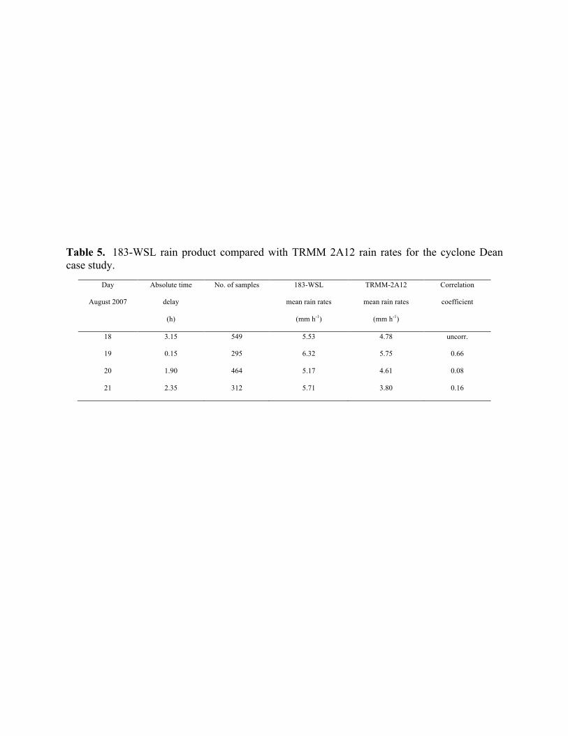
Table 5. 183-WSL rain product compared with TRMM 2A12 rain rates for the cyclone Dean case study.

Day

August 2007

Absolute time

delay

(h)

No. of samples 183-WSL

mean rain rates

(mm h-1)

TRMM-2A12

mean rain rates

(mm h-1)

Correlation

coefficient

18 3.15 549 5.53 4.78 uncorr.

19 0.15 295 6.32 5.75 0.66

20 1.90 464 5.17 4.61 0.08

21 2.35 312 5.71 3.80 0.16

Fig.1. 1 June 2007, 1550 UTC. NOAA-15/AMSU-B imagery at 183.31± 1 GHz (a), 183.31± 3 GHz (b) and 183.31± 7 GHz (c) of severe storms over Italy. The volume scattering of ice particles affects particularly the 190 GHz channel whose TBs were depressed of about 70 K with respect to the nominal values. Moreover, considering the peak of the weighting function of these channels it appears that the convective tower extended up to 8 km.

Fig. 2. 24 February 2004, 0140 UTC. NOAA-16/AMSU-B TB maps at 183.31± 1 GHz (a), 183.31± 3 GHz (b) and 183.31± 7 GHz (c). The cold and dry atmosphere allows for discriminating snow covered surfaces on the Alps, the Apennines and the Balkans. The bright and rough surface scatters the signal at 190 GHz by depressing TBs down by 70 K and at the adjacent frequency at 186 GHz where the reduction is quite modest especially on the lower mountain tops. Note the similarity with Fig. 1 where ice hydrometeors induce the same brightness temperature depression at 190 GHz that is caused in this case by the snow cover on the ground.

Fig 3. Flow chart of the 183-WSL algorithm: 1) Ingestion, processing, land/sea discrimination; 2) Module 183-WSLWV for water vapour and snow cover filtering; 3) Modules 183-WSLC and 183-WSLS for convective and stratiform rain classification, respectively; 4) Module 183-WSL for total rain rate estimation.

Fig. 4. Scatter plot of rainy vs clear sky TBs over the ocean using RTTOVSCAT for 9500 ECMWF different atmospheric profiles: a) 89, and b) 150 GHz.

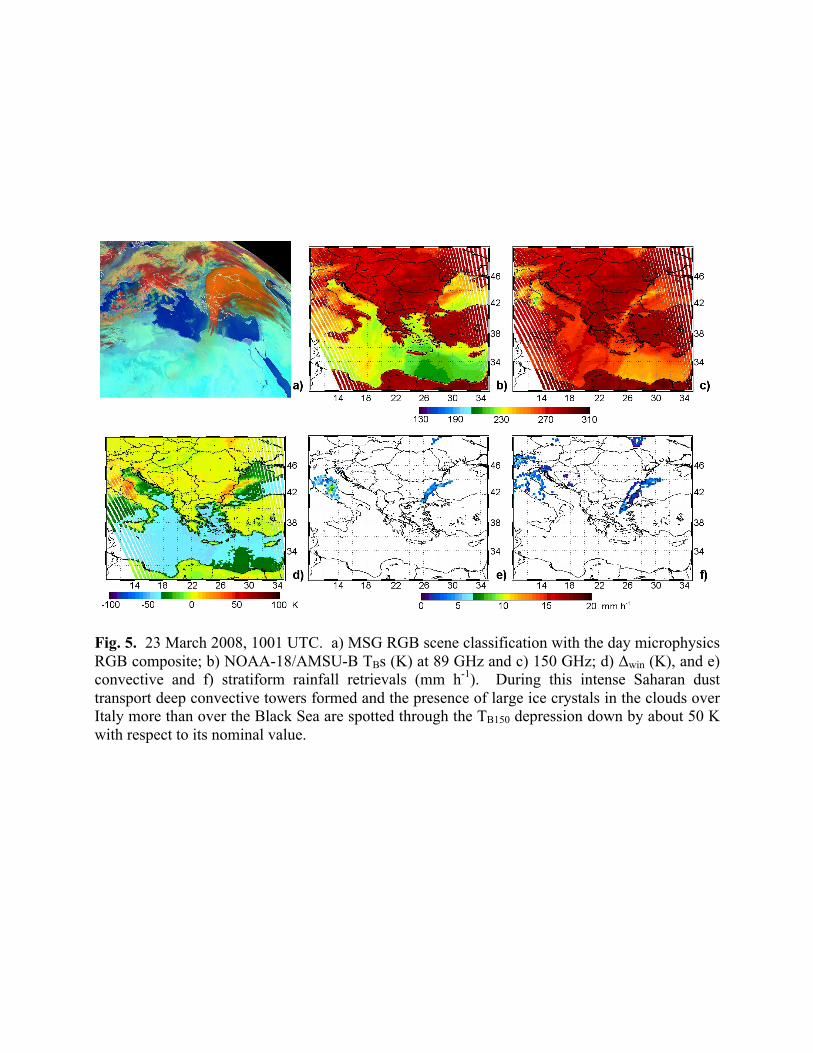
Fig. 5. 23 March 2008, 1001 UTC. a) MSG RGB scene classification with the day microphysics RGB composite; b) NOAA-18/AMSU-B TBs (K) at 89 GHz and c) 150 GHz; d) Δwin (K), and e) convective and f) stratiform rainfall retrievals (mm h-1). During this intense Saharan dust transport deep convective towers formed and the presence of large ice crystals in the clouds over Italy more than over the Black Sea are spotted through the TB150 depression down by about 50 K with respect to its nominal value.

Fig. 6. 14 June 2007, 1535 UTC, severe storm over eastern France. Comparison between the 183-WSL product without (a) and with (b) the 183-WSLW module. Without the water vapour module several areas are flagged as precipitating, but the attribution is fake.

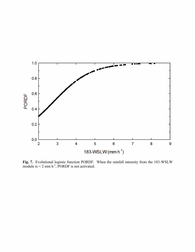
Fig. 7. Evolutional logistic function PORDF. When the rainfall intensity from the 183-WSLW module is < 2 mm h-1, PORDF is not activated.

Fig. 8. 10 June, 2007. Distribution of MSG SEVIRI TBs at 10.8 µm vs the 183-WSLW rain rate values. The dots are the observed values while the four lines represent the best fits. The time is that of the MSG-SEVIRI scan over the area.

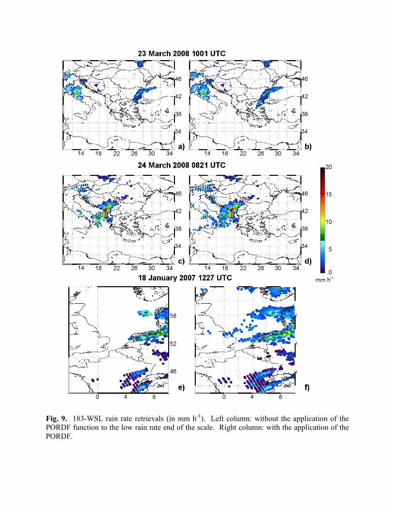
Fig. 9. 183-WSL rain rate retrievals (in mm h-1). Left column: without the application of the PORDF function to the low rain rate end of the scale. Right column: with the application of the PORDF.

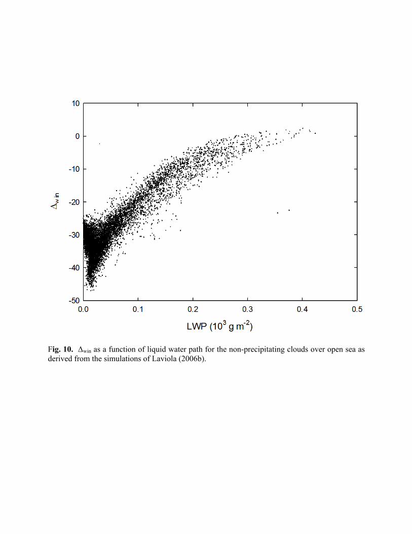
Fig. 10. Δwin as a function of liquid water path for the non-precipitating clouds over open sea as derived from the simulations of Laviola (2006b).

Fig. 11. 17 January 2007 1041 UTC. Stratiform rain over the open sea (English Channel and North Sea): a) 183-WSL rainfall retrieval (mm h-1), and b) 183-WSL LWP retrieval (103 g m-2). Note the increasing LWP values from the outer part of the cloud systems towards the centre where stratiform rain starts in correspondence of the LWP threshold value of 0.5 × 103 g m-2.

Fig. 12. 17 January 2007 1415 UTC, stratiform rain over Belgium; rain intensity is in mm h-1. a) SEVIRI TB at 11µm (MSG-TB11), b) Scattering Index (SI), c) 183-WSL, d) 183-WSLS, e) 183-WSLC, f) 183-WSLW, g) scatter plot 183-WSL vs rain products the MSG-TB11, h) 183-WSLS vs MSG-TB11, i) 183-WSLC vs SI, l) 183-WSLW vs MSG-TB11. Since the event is classified as quasi-stratiform the comparison between the 183-WSL and 183-WSLS rain maps shows a strong similarity. The large amount of water vapour sensed by the 183-WSLW module is correctly removed by the final retrieval.

Fig. 13. Severe storms over Italy, 10 and 12 June 2007. First four rows refer to the output of the 183-WSL and its modules (in mm h-1). The last two are the output of the MSG Precipitation Index (PI) and of the Scattering Index (SI) (in K). Note that the retrieval of the 183-WSLW module in mm h-1, but refers to pixels that are discarded in the final rainfall computation; some of them are retained by the PORDF application (see text for details).

Fig 14. Scatter plots for the three case studies of Fig. 13, one per row: a) and b) 10 June2007 1427 UTC; c) and d) 12 June 20071557 UTC; e) and f) 12 June 2007 2042 UTC. The scatter plots on the left of each case study show the comparison between the 183-WSL (black dots) and 183-WSLS (empty dots) retrievals vs the MSG Precipitation Index (PI). The scatter plots on the right column compare the 183-WSLC retrievals vs the Scattering Index (SI) values.

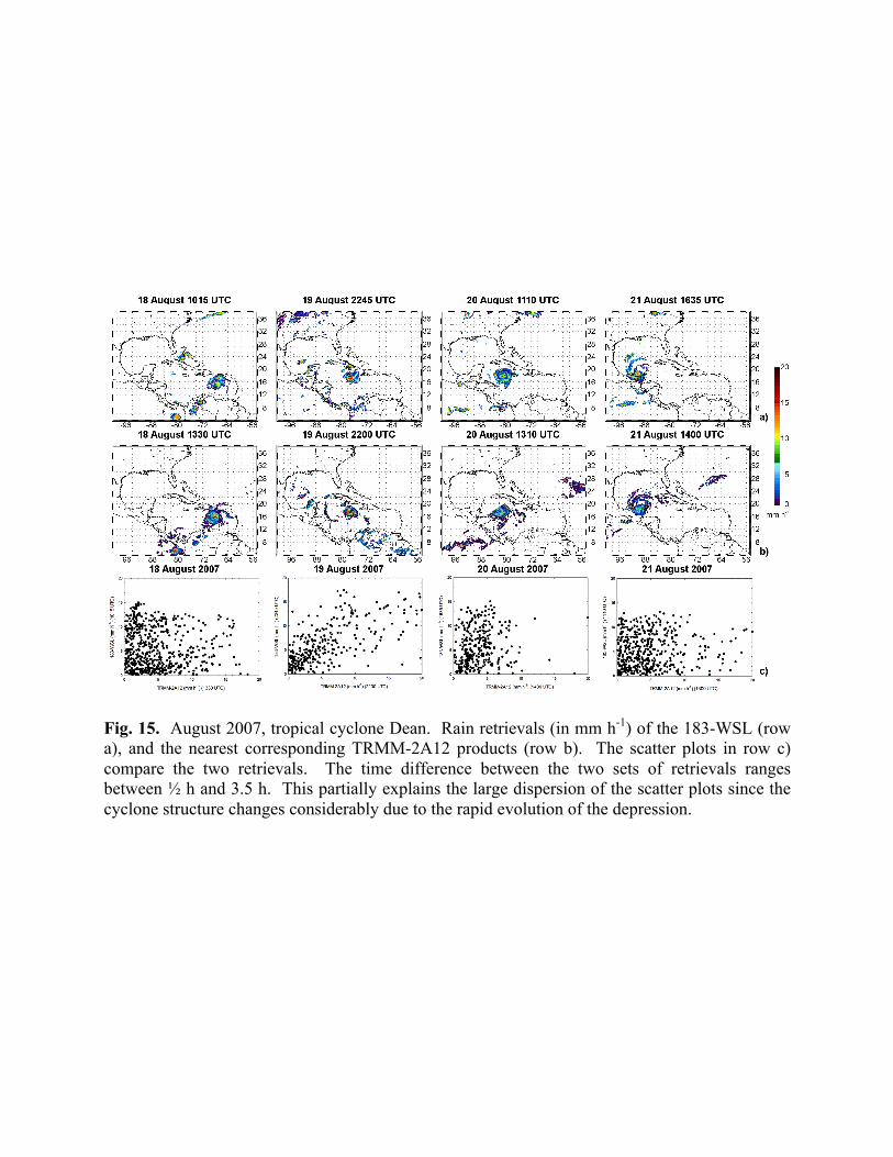
Fig. 15. August 2007, tropical cyclone Dean. Rain retrievals (in mm h-1) of the 183-WSL (row a), and the nearest corresponding TRMM-2A12 products (row b). The scatter plots in row c) compare the two retrievals. The time difference between the two sets of retrievals ranges between ½ h and 3.5 h. This partially explains the large dispersion of the scatter plots since the cyclone structure changes considerably due to the rapid evolution of the depression.