Development and application of a multisite rainfall stochastic downscaling framework for climate...

ClickHere

for

FullArticle

Development and Application of a Multisite Rainfall StochasticDownscaling Framework for Climate Change Impact Assessment

R. Mehrotra1 and Ashish Sharma1

Received 23 July 2009; revised 17 December 2009; accepted 26 February 2010; published 22 July 2010.

[1] The coarse resolution of general circulation models (GCMs) necessitates use ofdownscaling approaches for transfer of GCM output to finer spatial resolutions for climatechange impact assessment studies. This paper presents a stochastic downscaling frameworkfor simulation of multisite daily rainfall occurrences and amounts that strive to maintainpersistence attributes that are consistent with the observed record. At site, rainfalloccurrences are modeled using a modified Markov model that modifies the transitionprobabilities of an assumed Markov order 1 rainfall occurrence process using exogenousatmospheric variables and aggregated rainfall attributes designed to provide longer‐termpersistence. At site rainfall amounts on wet days are modeled using a nonparametric kerneldensity simulator conditional on previous time step rainfall and selected atmosphericvariables. The spatial dependence across the rainfall occurrence and amounts is maintainedthrough spatially correlated random numbers and atmospheric variables that are commonacross the stations used. The proposed framework is developed using the current climate(years 1960–2002) reanalysis data and rainfall records at a network of 45 rain gauges nearSydney, Australia, while atmospheric variable simulations of the CSIRO Mk3.0 GCM(corresponding to Intergovernmental Panel on Climate Change (IPCC) Special Report onEmission Scenarios (SRES) B1, A1B and A2 emission scenarios) are used for downscalingof rainfall for the current and future (year 2070) climate conditions. Results of the studyindicate wetter autumn and summer and drier spring and winter conditions over theregion in a warmer climate. The best estimates of annual rainfall project little change inthe number of wet days and slight increase (2% in 2070) in the rainfall amount. An increase(about 4%) in daily rainfall intensity (rain per wet day) is estimated in year 2070. Changesin rainfall intensity, wet and dry spells, and rainfall amount in wet spells suggest that thefuture rainfall regime will have longer dry spells interrupted by heavier rainfall events.

Citation: Mehrotra, R., and A. Sharma (2010), Development and Application of a Multisite Rainfall Stochastic DownscalingFramework for Climate Change Impact Assessment, Water Resour. Res., 46, W07526, doi:10.1029/2009WR008423.

1. Introduction

[2] General circulation models (GCMs) are widely used tosimulate the present and future climates under assumedgreenhouse gas emission scenarios, both in space and time[e.g., IPCC, 2007; Bergström et al., 2001; Varis et al. 2004].One of the key limitations of GCM simulations is the coarsegrid resolution at which they are run. As a result, they areincapable of representing local subgrid‐scale features anddynamics that are often required for impact studies, especiallyat a catchment scale [IPCC, 2007; Charles et al., 2004;Vicuna et al., 2007]. Consequently, techniques have beendeveloped to transfer the GCM output from coarse spatialscales to local or regional scales by means of downscaling.These downscaling techniques can be classified into twocategories: “dynamical downscaling” that uses regional cli-mate models (RCMs) to simulate finer‐scale physical pro-cesses [e.g., Giorgi et al., 2001; Mearns et al., 2001, 2004;

Fowler et al., 2007] and “statistical downscaling” that is basedon developing statistical relationships between the regionalclimate and preidentified large‐scale parameters [e.g., Wilbyet al., 2004; Mehrotra and Sharma, 2005; Vrac and Naveau,2007]. A diverse range of statistical downscaling techniqueshas been developed over the past few years, with mostfalling into a category where the responses (precipitation)are related to predictors (coarse scale atmospheric and localscale time‐lagged variables) or into a category where theresponses are related to a discrete or continuous state, whichis modeled as a function of the atmospheric and local scalepredictors [Hewitson and Crane, 1996; Wilby and Wigley,1997; Hughes et al., 1999; Charles et al., 2004; Bartholyet al., 1995; Stehlík and Bárdossy, 2002; Mehrotra andSharma, 2005; Vrac and Naveau, 2007]. There are limita-tions and assumptions involved in both techniques that con-tribute to the uncertainty of results [see also Yarnal et al.,2001; Fowler et al., 2007]. Yarnal et al. [2001], Charleset al. [2004], IPCC [2007], and Fowler et al. [2007] pro-vide good reviews and discussions of various downscalingtechniques.[3] In general, GCMs (and hence the resulting downscaled

outputs to some extent) tend to undersimulate year‐to‐year

1Water Research Center, School of Civil and EnvironmentalEngineering, University of New South Wales, Sydney, Australia.

Copyright 2010 by the American Geophysical Union.0043‐1397/10/2009WR008423

WATER RESOURCES RESEARCH, VOL. 46, W07526, doi:10.1029/2009WR008423, 2010

W07526 1 of 17

http://dx.doi.org/10.1029/2009WR008423

(low‐frequency) variability in rainfall and poorly representextreme events, when compared to the historical climaterecord [Ines and Hansen, 2006; Knutti, 2008], implying thatthe probability of sustained droughts or periods of high flowsalso are likely to be underestimated in future climate pro-jections. This has significant implications in water resourceplanning and design, with undersimulation of sustaineddroughts resulting in significantly overestimated reservoiryields, artificially enhancing the reliability associated withour existing water supply infrastructure to sustain futuredemands [Milly et al., 2008]. Similarly, undersimulatedpersistence in rainfall also implies reduced variations incatchment conditions prior to design rainfall events, leadingto floods that do not exhibit the low‐frequency multidecadalvariability often observed in Australian records [Micevskiet al., 2006], increasing the uncertainty associated with thespecification of a design flood for future infrastructuredevelopments. There is a need to address this limitation in thedownscaled rainfall outputs for them to be of use in a waterresources context.[4] Commonly used approaches to match the observed

variability in the downscaled climate variables include vari-ance inflation, expanded downscaling, and randomization.Variance inflation [Karl et al., 1990] increases the variabilityby multiplying the downscaled simulations by a suitablefactor, however, is of limited use in case of daily rainfallowing to large number of zeros in the rainfall record. Also, themethod assumes that all climate variability is related to thelarge‐scale predictor fields. Another approach is of “ran-domization” where additional variability is added in the formof white noise [von Storch, 1999].Kyselý [2002] reports goodresults in the reproduction of 20 to 50 year return periodvalues of central European surface temperature using thisprocedure. The “expanded downscaling” approach is devel-oped by Burger [1996] and has been used by Huth [1999],Dehn et al. [2000], and Muller‐Wohlfeil et al. [2000]. Acomparison of the three methods notes that each presentsdifferent problems [Burger and Chen, 2005]. Varianceinflation poorly simulates spatial correlations, while ran-domization performs well for control climate simulations butis unable to reproduce changes in variability, which may limitthe use of the approach for climate change impact studies.Expanded downscaling is sensitive to the choice of statisticalprocess (a variant of canonical correlation analysis) used inits formulation.[5] Recently, there have been many studies assessing the

ability of RCMs to reproduce more plausible climate changescenarios for extreme events and climate variability at theregional scale [e.g., Christensen et al., 2007; Fowler et al.,2005; Frei et al., 2006; Schmidli et al., 2007], but we focuson stochastic downscaling in this study.[6] The use of statistical/stochastic downscaling to repro-

duce short‐ as well as long‐term frequency components inthe downscaled rainfall has been attempted in the past byemploying combinations of rapidly varying and slowly vary-ing atmospheric circulation variables or by conditioning dailyweather generator parameters on indices of atmospheric cir-culation [Cavazos, 1997;Wang andConnor, 1996;Wilby et al.,2002; Woolhiser et al., 1993]. For example, Cavazos [1997]uses the Pacific North American, El Niño–Southern Oscil-lation (ENSO) index and 1000–500 hPa thickness indices tomodel monthly rainfall totals in NE Mexico. Woodhouse[1997] considers six large‐scale climate indices to model

winter rain days and maximum temperatures at multiplestations in the United States. Wilby et al. [2002] comparethree downscaling models using daily precipitation data ofUnited Kingdom for sites located in the regions of strongestNorth Atlantic forcing. The parameters of first model areimplicitly conditioned by three regional airflow indices;while the parameters of the second model are explicitly con-ditioned by either the North Atlantic Oscillation (NAO)index or sea surface temperature (SST) anomalies and dailyvorticity; and finally, the parameters of the last model areunconditional. They conclude that the conditional modelsdisplay greater skill for monthly rainfall statistics relative tounconditional model, and explicit conditioning offers addi-tional advantages for the chosen sites and seasons of greatestforcing. Similarly, Katz and Parlange [1993, 1996] use twodiscrete states of monthly mean sea level pressure to con-dition the January daily precipitation parameters and reportthat the conditional model reproduces the variance of totalmonthly precipitation. Kiely et al. [1998] condition theoccurrence and intensity parameters of a daily precipitationmodel on the multistate indices of mean monthly sea levelpressure and geostrophic wind directions at Valentia, Ire-land, and find improved estimates of the site’s standarddeviation of monthly precipitation in relation to the uncon-ditional model. Wilby [1998] reports encouraging results indownscaled monthly precipitation diagnostics for two sitesin the United Kingdom by using the NAO index and SSTanomalies to continuously condition the parameters of astochastic rainfall model. However, the improvements arelimited to specific seasons and locations according to thechoice of low‐frequency predictor(s).[7] The performance of downscaling methods varies

across seasons, locations, GCMs, and depends strongly onbiases inherited from the driving GCM and the presence andstrength of regional scale features such as orography, prox-imity to sea, and land use and vegetation. In general, statis-tical downscaling methods are more appropriate where pointvalues of extremes are needed for impact studies. Consider-ation of these analyses suggests that, at least for present‐dayclimates, dynamical downscaling methods provide littleadvantage over statistical techniques [Fowler et al., 2007].[8] This paper presents a stochastic downscaling frame-

work for simulation ofmultisite daily rainfall occurrences andamounts, which is capable of maintaining persistence attri-butes that are consistent with the observed record. Theframework operates in two stages: (1) the downscaling ofrainfall occurrences (whether rain or no rain) and (2) down-scaling of rainfall amounts on days simulated as wet in thefirst stage. The rainfall occurrence downscaling model is avariation of the stochastic generation‐modified Markovmodel (MMM) [Mehrotra and Sharma, 2007b], facilitatingthe use of exogenous atmospheric predictors and local low‐frequency variability indicators so as to simulate properly thesustained extreme events and year‐to‐year variations in thedownscaled rainfall occurrence field. At site rainfall amountson wet days are simulated using a kernel density estimation‐based approach (hereafter referred to as KDE) that also allowsproper representation of temporal dependence attributes.Spatial dependence in rainfall occurrence and amounts fieldsis maintained by making use of random innovations that arespatially correlated yet serially independent in nature [Wilks,1998]. The smooth transition from one season to anotheras well as estimation of transition probabilities, conditional

MEHROTRA AND SHARMA: A MULTISITE RAINFALL STOCHASTIC DOWNSCALING W07526W07526

2 of 17

densities, spatial correlations, skewness, and other variablesfor each day is achieved by using the concept of a movingwindow [Harrold et al., 2003;Mehrotra and Sharma, 2005].[9] The rainfall occurrence downscaling model MMM

proposed here departs from the commonly used weathergenerators in a sense that transition probabilities or theparameters of the model are updated at each time step on thebasis of the past rainfall behavior and the current time stepvalues of the atmospheric variables. Thus, providing a morelogical and refined way of incorporating the low‐frequencyvariability and the influence of atmospheric variables in thedownscaled results. Rather than using mixture of discretestochastic processes [Katz and Parlange, 1993, 1996] orcontinuous regression relationship [Wilby, 1998;Wilby et al.,2002], the proposed approach explicitly considers the com-bined effect of atmospheric variables influencing the climateand of the longer‐term wetness state characterizing the low‐frequency variability. We expect that owing to the parameterupdating procedure at each time step, it should adapt better tothe changes that are expected to occur in the future. It alsodeviates from the logic of weather state‐based models likenonhomogeneous hidden Markov model, NHMM [Hughesand Guttorp, 1994] and nonparametric nonhomogeneoushidden Markov model, NNHMM [Mehrotra and Sharma,2005] and weather state downscaling model of Vrac andNaveau [2007] as rainfall occurrences are considereddirectly conditional upon the atmospheric variables, thereby,evading the use of discrete or continuous weather states.Additionally, the model provides a better representation ofthe observed low‐frequency variability and spell extremes byincorporating the behavior of the climate over the recent pastperiods.[10] The downscaling framework comprising of the MMM

rainfall occurrence simulator and the KDE rainfall amountsimulator, is referred hereafter as MMM‐KDE. This frame-work is initially calibrated using reanalysis atmospheric dataand observed daily rainfall (1960–2002) at 45 rain gaugeslocated around Sydney, Australia, and subsequently validatedusing current climate GCM data. The model performance isevaluated on the basis of reproduction of a few importantrainfall attributes representing at site temporal and across sitespatial dependencies. We also demonstrate the improvementsoffered by including the aggregated wetness state predictor inthe rainfall occurrence downscaling model. Finally, themodel is applied to downscale daily rainfall for year 2070 andchanges in rainfall behavior evaluated.

[11] The paper is organized as follows. The methodologyand the models used are discussed and described in section 2.Details on the application of models considered, data, andstudy region used are presented in section 3. This is followedby a description of the downscaled results obtained for cur-rent and future climates, in section 4. We conclude the paper

by presenting the summary and conclusions drawn from theresults, in section 5.

2. Methodology

[12] In the discussions that follow, all multivariable vectorsor matrices are expressed as bold and single variables orparameters using nonbold characters or symbols. We denoterainfall occurrence at a location k and time t as Rt(k) and at thepth time step before the current as Rt–p(k). Also, a ns‐siterainfall occurrence vector at time t is denoted as Rt and avector of predictor variables (consisting of atmosphericand/or other relevant indicators) as Zt. Unless explicitlyspecified, hereafter, the term rainfall represents rainfallamount. The following subsections describe the rainfalloccurrence and amount models and the procedure that wasused to incorporate the spatial dependence in the downscaledoccurrence and amount series.

2.1. Downscaling of Rainfall Occurrence Using MMM

[13] The general structure of the rainfall occurrencedownscaling model (MMM) is presented in the study ofMehrotra and Sharma [2007b] in a stochastic generationcontext and is described here in the context of downscaling.In general, the rainfall downscaling problem could be ex-pressed as the conditional simulation of Rt(k)∣Zt(k), whereZt(k) represents a vector of conditioning variables at a loca-tion k and at time t, that consists of atmospheric predictorvariables, lagged rainfall to assign daily or short‐term per-sistence, and derived rainfall indicators selected to impactspecific characteristics of interests. If Zt(k) comprises ofRt − 1(k) alone, then MMM reduces to a simple Markov order1 model, whereas addition of variables representing longertime scale persistence also, would reduce it to the stochasticrainfall generator presented in the study of Mehrotra andSharma [2007b].[14] In the following discussions, we present the parame-

terization ofRt(k)∣Zt(k) as a modulation of theMarkov order 1(or higher) transition probability representation by the impactof nondiscrete exogenous predictors. For brevity, site notationsare dropped in the subsequent discussions. The parameters (ortransition probabilities) of the Markov order 1 rainfall occur-rence process are represented as P(Rt∣Rt − 1). Inclusion ofnondiscrete predictors Xt in the conditioning vector Zt mod-ifies the transition probabilities to P(Rt∣Rt − 1, Xt), which canbe expressed as

The first term in (1) defines the transition probabilitiesP(Rt∣Rt − 1) of a first‐orderMarkovmodel (representing order 1dependence), while the second term signifies the effect ofinclusion of predictor set Xt in the conditioning vector Zt.If Xt consists of derived measures (typically linear combina-tions) of atmospheric variables and/or summation of number

P Rt ¼ 1 Rt�1 ¼ i;Xtjð Þ ¼ P Rt ¼ 1;Rt�1 ¼ i;Xtð ÞP Rt�1 ¼ i;Xtð Þ ¼ f Xt Rt ¼ 1;Rt�1 ¼ ijð Þ � P Rt ¼ 1;Rt�1 ¼ ið Þ

f Xt Rt�1 ¼ ijð Þ � P Rt�1 ¼ ið Þ

¼ P Rt ¼ 1;Rt�1 ¼ ið ÞP Rt�1 ¼ ið Þ � f Xt Rt ¼ 1;Rt�1 ¼ ijð Þ

f Xt Rt ¼ 1;Rt�1 ¼ ijð ÞP Rt ¼ 1 Rt�1 ¼ ijð Þ½ � þ f Xt Rt ¼ 0;Rt�1 ¼ ijð ÞP Rt ¼ 0 Rt�1 ¼ ijð Þ½ � ð1Þ


3 of 17

of wet days in prespecified aggregation time periods (asexplained later), one could approximate the associated con-ditional probability density f(Xt∣Rt = 1, Rt − 1 = i) using amultivariate normal distribution. Consequently, the condi-tional probability density f(Xt∣Rt = 1) as specified in (1) canbe expressed as a mixture of two multivariate normals. Thisleads to the following simplification:

where the m1,i represent the mean vector E(X∣Rt = 1, Rt − 1 = i)andV1,i is the corresponding variance‐covariance matrix, andsimilarly, m0,i and V0,i represent the mean vector and thevariance‐covariance matrix ofXwhen (Rt − 1 = i) and (Rt = 0),respectively. The parameters p1i represent the baseline tran-sition probabilities of the first‐order Markov model definedby P(Rt = 1∣Rt − 1 = i.) with p0i equaling (1 − p1i). The det()represents the determinant operation and T represents thetranspose operator. While the assumption of a multivariatenormal distribution simplifies the specification of the condi-tional probabilities in (2), this assumption may be inappro-priate for variables that are known to have skewed or othernon‐Gaussian traits. In such situations, use of some appro-priate transformation to convert the data back to normal maybe useful. However, it may be noted that most common datatransformation technique are developed for univariate casesonly while data set X as described here is multivariate, andtherefore, univariate normal transformation may not neces-sarily translate into multivariate normal. Alternatively, theconditional multivariate probabilities f(Xt∣Rt = 1, Rt − 1 = i)and f(Xt∣Rt = 0, Rt − 1 = i) of (1) may be estimated using anonparametric kernel density estimation procedure asdescribed next.[15] For a d‐dimensional multivariate Gaussian kernel, the

conditional multivariate density f(Xt∣Rt, Rt − 1) at a time step tcan be written as:

f Xt Rtj ¼ j;Rt�1 ¼ ið Þ ¼ 1

N

XNk¼1

1

2�ð Þd=2�d det Sð Þ1=2

� exp � Xt � Xkð ÞS�1 Xt � Xkð Þ2�2

� �; ð3Þ

where Xk is kth multivariate data point of X under thecondition that (Rt = j (0 or 1), Rt − 1 = i) and N is number ofsuch data points. f(Xt∣Rt, Rt − 1) is the estimated conditionalmultivariate probability density expressed as a weightedsum of N Gaussian density functions each with a mean Xk

and covariance l2S, where, S is a sample covariance of dataset X when (Rt = j (0 or 1), Rt − 1 = i), and l is a smoothingparameter, known as the bandwidth of the kernel densityestimate.[16] A simplistic choice of bandwidth, the Gaussian ref-

erence bandwidth [Scott, 1992] is considered as appropriate

and optimal if the underlying probability density is Gaussian.However, when modeling variables exhibiting significantskewness, assuming aGaussian distribution and assuming thevariance associated with each kernel (or each observation) tobe the same, may not be appropriate. In such situations,varying the bandwidth depending on the associated obser-vation helps characterizing the probability more meaning-

fully, especially in regions where there may be many ob-servations (requiring a smaller bandwidth) or where theremay be few (requiring a larger bandwidth). The local Gammabandwidth lXk

for the kth data point of the individual vari-ables inX series is written as [Mehrotra and Sharma, 2007a]:

�Xk ¼1

2ffiffiffi�

pf Xkð Þ �2 � 2� � � 1ð Þ

Xkþ � � 1ð Þ � � 2ð Þ

X 2k

� �20BBB@

1CCCA

1= dþ4ð Þ

� N �1= dþ4ð Þð Þ; ð4Þ

where f(Xk) is the Gamma density at Xk, g and h, respectively,are the scale and shape parameters of the Gamma distributionfor the variable being modeled (resulting in different localbandwidths associated with individual variables in X), N isagain the number of observations in X when (Rt = j (0 or 1),Rt − 1 = i), d is the number of predictor variables, and lXk

beingequivalent to l of equation (3). Further details on the deri-vation of equation (4) are given by Mehrotra and Sharma[2007a] while derivation of equation (3) and further discus-sions related to the kernel density procedure are given bySharma and O’Neill [2002] and Mehrotra and Sharma[2007a, 2007b].[17] In the present application, we consider the nondiscrete

conditioning vector X (for rainfall occurrence downscaling)as consisting of variables representing selected atmosphericvariables and long‐term persistence indicators formulated asaggregate wet days preceding the current time step. Param-eters of MMM are estimated on a daily basis using either (2)or (3) depending on the joint distribution of predictor vari-ables inX. In order to save computer time, the switching fromparametric to nonparametric multivariate density estimation(which requires significantly greater computational effortsthan the parametric case) at each time step is decided on thebasis of average skewness of the data set X. If the averageskewness is less than 0.3 then the parametric approximationis used; otherwise, the nonparametric procedure is used toestimate the conditional multivariate density.

2.2. Formation of Aggregated Wetness State

[18] A vector of aggregated rainfall Xrt representing thewetness over the recent past can be expressed as [following

P Rt Rt�1j ;Xtð Þ ¼ p1i

1

det V1;i

� �1=2 exp � 1

2Xt � �1;i

� �V�1

1;i Xt � �1;i

� �T

1

det V1;i

� �1=2 exp � 1

2Xt � �1;i

� �V�1

1;i Xt � �1;i

� �T p1i

" #þ 1

det V0;i

� �1=2 exp � 1

2Xt � �0;i

� �V�1

0;i Xt � �0;i

� �T p0iÞ

" # ;

ð2Þ


4 of 17

Harrold et al., 2003; Sharma and O’Neill, 2002; Mehrotraand Sharma, 2007a, 2007b]:

Xrt 2 Xrj1 ;t;Xrj2;t; . . . ::;Xrjm ;t� �

; Xrji ;t ¼1

ji

Xjil¼1

Rt�l ; ð5Þ

where m is the number of such predictors and Xrji,t describeshow wet it has been over the preceding ji days with Rt − 1

representing rainfall occurrence. This aggregated wetnessstate, by formulation, assumes values between 0 and 1 that areincreasingly continuous as the aggregation period ji increases.Please note that the aggregated wetness state is calculatedseparately for each station.

2.3. Downscaling of Rainfall Amounts

[19] A nonzero rainfall amount (with a rainy day definedusing a threshold of 0.3 mm/d followingHarrold et al. [2003]andMehrotra et al. [2004]) must be simulated for each day ateach location that the MMM occurrence downscaling modelsimulates as wet. Additionally, the downscaled rainfallamount series (for the current climate) should representaccurately the spatial and temporal dependence present in theobserved rainfall record. The downscaling of rainfall amountis based on the kernel density procedure similar to what hasbeen described in section 2.1. The amounts model down-scales the rainfall at individual stations conditional on theselected atmospheric variables as well as the previous days’rainfall. As rainfall amounts are downscaled independently ateach location, observed spatial dependence across the stationsis not directly reproduced. This is introduced by making useof spatially correlated random numbers as described insection 2.4. In addition to this, a local wetness fraction (asdefined later in section 3.2) is used to enforce smooth spatialcontinuity across the realizations. The use of rainfall amounts

on the previous day as a conditioning variable provides aMarkov order 1 dependence to the downscaled series. Furtherdetails on the general structure of the KDE model are avail-able in Mehrotra and Sharma [2007a, 2007b].

2.4. Modeling Spatial Dependences in RainfallOccurrence and Amounts

[20] As discussed in the above sections, stochastic down-scaling of rainfall occurrences or amounts for a given locationproceeds through simulation from the associated conditionalprobability (or transition probability) distribution indepen-dently. The method used to incorporate spatial dependencein such simulations over many point locations involves usinguniform random variates that are independent in time butexhibit a strong dependence across the multiple point loca-tions considered. Denote ut as a vector of uniform [0,1]variates of length ns at time step t, with ns being the numberof stations. The vector ut (≡ ut (1), ut (2),……ut (ns)) isdefined such that for locations k and l, corr[ut(k), ut + 1(k)] = 0(or, random numbers are independent across time) butcorr[ut(k), ut(l)] ≠ 0 (or, random numbers are correlated acrossspace). As a result, there is spatial dependence between indi-vidual elements of the vector ut, this dependence being intro-duced to induce observed spatial dependence in the responsevariables they are used to simulate. More details on thisapproach are given byWilks [1998] andMehrotra et al. [2006].

3. Application of Downscaling Model

[21] This section presents the details on the data and thestudy area and the selection of model parameters for down-scaling framework.

3.1. Data sets, Study Area, and Variables

3.1.1. Study Area[22] The study region is located around Sydney, eastern

Australia spanning between 149°E–152°E longitude and32°S–36°S latitude (Figure 1). The physiogeographicalconditions near Sydney cause large climatic gradients evenover short distances, e.g., from lowland areas to mountainregions and from the coast to the inland. Most significantrainfall events in winter in this region involve air masses thathave been brought over from the east coast low‐pressuresystems. Orographic uplift of these air masses when theystrike coastal ranges or the great dividing range often pro-duces very heavy rain. Several of the most severe floodsexperienced east of the great dividing range have resultedfrom east coast low‐pressure systems. In summer, tropicaldepressions moving southward from Queensland into NewSouth Wales bring warm, cloudy, and drizzly weather tocoastal regions of eastern Australia. These conditions canresult in heavy rainfall if some means of lifting is available.3.1.2. Rainfall[23] For this study, a 43‐year continuous record (from

1960 to 2002) of daily rainfall at 45 stations around Sydney(Figure 1) is used. The study area therefore has both thepreconditions to develop stochastic downscaling models andthe need to apply them, adding value to the coarse climatescenarios provided by global climate models.3.1.3. Large Scale Observed Atmospheric Variables[24] The required observed atmospheric variables for

25 grid points over the study area are extracted from the

Figure 1. Reanalysis and CSIRO GCM data grids andstudy region.


5 of 17

National Center for Environmental Prediction (NCEP)reanalysis data provided by the NOAA‐Cooperative Institutefor Research in Environmental Sciences, Climate DiagnosticsCenter, Boulder, Colo, from theirWeb site at http://www.cdc.noaa.gov/. These variables are available on 2.5° latitude ×2.5° longitude grids on a daily basis for the same period as therainfall record (Figure 1). As an observed rainfall valuerepresents the total rainfall over a 24 hour period ending at0900 hours (local time, LT) in the morning, the availableatmospheric measurements on the preceding day are con-sidered as representative of current day’s rainfall. Thesedata are regridded from the 25 NCEP grids (2.5° latitude ×2.5° longitude) to the 9 CSIRO climate model grids(3.73° latitude × 3.75° longitude) prior to the predictoridentification and model fitting exercises as the output fromthe CSIRO global climate model forms the basis whenstatistical downscaling is applied to produce local climatescenarios for current (1960–2002) and future conditions(2061–2080) (Figure 1). For defining a grid‐averaged valueand North–South and East–West gradients, all 9 grid pointvalues are used to smoothen out the bias and spatial shifts,if any, at an individual grid point values.3.1.4. Large‐Scale GCM Variables[25] Runs of Commonwealth Scientific and Industrial

Research Organization (CSIRO), Australia Mark3 GCM[Gordon et al. 2002] for the three emission scenarios SRESB1, A1B, and A2 [IPCC 2007] are considered in the presentstudy. The required information about atmospheric variablesfor current and future climates, as an output of Mark3 GCM,is provided by the Atmospheric Research Division of theCSIRO. The atmospheric component of the CSIRO Mark3coupled model has a horizontal resolution of T63 (approxi-mately 1.875° longitude × 1.875° latitude) and 18 verticallevels. A detailed description of the physical representationsin the CSIRO Mark3 is given by Gordon et al. [2002].[26] GCM data sets of atmospheric variables for the base-

line (covering a 43 year period between 1960 and 2002 andrepresenting the current climate) and the future climate by2070 (2061–2080) periods are considered in the analysis.For mean sea level pressure, single daily observations at0000 hours GMT while for the remaining variables twice‐daily observations at 0000 hours and 1200 hours GMT areavailable. These variables are extracted from a single con-tinuous (transient) run (corresponding to each of the threeSRES emission scenarios) for the grid nodes over the studyregion. Again, as an observed rainfall value represents thetotal rainfall over a 24 hour period ending at 0900 hours (localtime, LT) in the morning, similar to the reanalysis data, theavailable atmospheric measurements on the preceding day areconsidered as representative of current day’s rainfall. Formeansea level pressure, observation at 0000 hours GMT while forother variables average of 0000 hours and 1200 hours GMTvalues on the preceding day is adopted.[27] The climate change studies commonly focus on the

years 2030, 2050, 2070, or even 2100 for assessing theimpacts of climate change in the future. It is argued thatthe climate projections too far into the future may not berealistic, at least with the models available at the present timepartly because population projections and related develop-ments have generally been made (which are somewhat reli-able) only until year 2050 (year 2025, in most cases), whichalso forms an important basis for future emission scenarios;and the IPCC [2007] considers mostly year 2030 (perhaps a

possible “change point”) in their assessment of climatechange impacts for Australia (and also New Zealand), espe-cially for water resources and agriculture. However, on otherhand, it is believed that the most GCMs show large uncer-tainties in the projected regional climate changes for 2030mostly due to differences between the results of the climatemodels rather than the different emission scenarios [Hennessyet al., 2008]. In the present study, results reported later arederived for year 2070 only under the assumption that theresults for 2070 are much more strongly affected by emis-sions rather than model uncertainties.3.1.5. Adjustment of GCM Data[28] A preliminary comparison of current climate GCM

and corresponding reanalysis atmospheric fields (1960–2002) on the basis of calendar day means (average across allyears), standard deviations, and distribution plots suggestsubtle differences in these characteristics. This necessitatessome scaling to be carried out on the GCM data in order toremove the regional bias in the data. We adjust the GCMdata for the baseline (1960–2002) and future climate period(2061–2080) by adopting a two‐stage adjustment procedure.In the first stage, the GCM series (current and future climates)is corrected for bias in the mean by subtracting the mean ofthe baseline period GCM data and adding the mean of thebaseline period reanalysis data. In the second stage, themean‐corrected GCM series (for current and future climates) isrescaled to correct for bias in standard deviation withoutaffecting the mean. This is achieved by first subtracting themean (of the mean‐corrected series) and then rescaling theresulting data series by the ratio of the standard deviations ofthe reanalysis data and baseline period GCM data, with thefinal step being the readdition of the mean (of the mean‐corrected series) thereafter. This ensures that any biases in theGCM atmospheric fields are removed before their use fordownscaling while the mean shift from current to future cli-mate is maintained. Means and standard deviations for thestandardization procedure are estimated on a daily basis byconsidering a moving window of 31 days centered on thecurrent day. The daily time scale is found to provide a betteragreement of various spatial and temporal attributes ofobserved and downscaled rainfall in comparison to monthlyor seasonal scale. The standardization procedure helpsremoving the mean bias from the raw data and reducing thedifferences in the first two moments of the reanalysis and thealtered GCM series.3.1.6. Identification of Significant Predictors[29] There is little consensus on the most appropriate

choice of predictor variables. Atmospheric circulationstrongly influences the local climate. Nevertheless, the abilityof circulation indices alone to account for long‐term ordecadal variability for temperature and also for precipitation,varies with time [Hanssen‐Bauer and Forland, 2000;Benestad, 2001]. Additional predictors therefore have to beincluded not only to project a possible future climate changebut also to describe climate development in the past. Whenthe downscaled response is precipitation, inclusion of a pre-dictor variable representing atmospheric moisture is foundto provide better results [Yarnal et al., 2001, Charles et al.1999]. Trenberth et al. [2003] argue that the main changesin rainfall to be experienced in future will be due to betteravailability of moisture in the atmosphere, leading to higherrainfall rates and greater intervals between rain events.Harpham andWilby [2005] found specific humidity, whereas


6 of 17

Martin et al. [1997] and Easterling [1999] found relativehumidity as a good indicator of precipitation. Buishand et al.[2004] suggested using relative humidity for precipitationoccurrence and specific humidity for precipitation amounts asrepresentatives of atmospheric moisture.Charles et al. [1999]suggest using difference of air and dew point temperatures asa predictor for rainfall occurrences because it is an indicatorof relative moisture rather than absolute moisture. Similarly,Evans et al. [2004] advocate using difference of equivalentpotential temperatures at different pressure levels as one ofthe predictor to capture the instability of the atmosphere. Itmay, however, be noted that GCMs provide less accuratesimulations of moisture than of sea level pressure and geo-potential heights [Yarnal et al. 2001; Cavazos and Hewitson,2005].[30] On the basis of above discussions and the results of

earlier downscaling studies, we picked a large set of atmo-spheric predictors comprising of atmospheric circulation andmoisture variables at various levels and their horizontal andvertical gradients as the potential predictors. The predictoridentification exercise is carried out at daily time step for eachseason (MAM, JJA, SON, DJF). To simplify the procedure,area‐averaged wetness fraction (average of rainfall occur-rences (0, 1) at all stations on a given day) for rainfalloccurrence and area‐averaged rainfall for rainfall amountprocesses is considered as a solo predictand in the predictoridentification exercise adopted here. As some of these pre-dictors might be highly correlated among themselves, aninitial screening is carried out to exclude the highly correlatedpredictors (having correlation higher than 0.90). This leads toonly a handful of potential atmospheric predictors. Finally, anonparametric stepwise predictor identification analysisbased on partial mutual information [Sharma, 2000] is carriedout to identify sets of significant atmospheric predictors foreach season and for the occurrence and amounts models.To account for the short‐term persistence in the rainfalloccurrence/amount downscaling process, the previous dayarea‐averaged wetness fraction/rainfall is included as a pre-identified predictor in the conditioning vector for each sea-son before carrying out the predictor identification exercise.For rainfall occurrence process, one additional preidentified

predictor, namely, the previous 365 days’ area‐averagedwetness state is also included. This predictor is identifiedbased on a sensitivity analysis and is found to improvesignificantly the representation of low‐frequency variabilityin the simulated rainfall [Mehrotra and Sharma, 2007b].Table 1 provides the list of atmospheric predictors identifiedas significant for occurrence and amount processes and forall seasons.

3.2. Selection of Model Parameters

[31] For rainfall occurrence downscaling model (MMM),we consider individual at site Markov order 1 models con-ditional on preidentified atmospheric variables (commonacross all stations) and the previous 365 days’ wetness state(for each site). To improve the representation of area averagedwetness fraction, the previous day’s area‐averaged localwetness fraction (ascertained using an inverse distancesquared weighting) is also included as a conditioning vari-able. Thus, the short‐term persistence in the downscaledrainfall is maintained through an order 1 Markovian structureand the localized previous day’s wetness fraction, while thelonger‐time scale persistence is introduced through the pre-vious 365 days’ wetness state, apart from the effect of theatmospheric predictors used. As the distribution of the localarea averaged previous day’s wetness fraction is found to behighly skewed rather than attempting a transformation, thetwo conditional probabilities of equation (1) for this variable,are estimated empirically, and an assumption made that thisvariable is independent of the remaining predictors. Therelationship between the correlations of the series of normallydistributed random numbers and corresponding simulatedrainfall occurrence and amounts at a station pair is ascertainedon a daily basis based on the observations that fall within amoving window of length 31 days centered on the currentday.[32] For rainfall amounts, it is observed that as the proce-

dure incorporating spatial dependence considers the corre-lations of rainfall amounts for each station pair with bothstations being wet, the distribution of downscaled rainfallamounts on occasions when only one station (of a stationpair) is wet, does not correspond well with observations. This

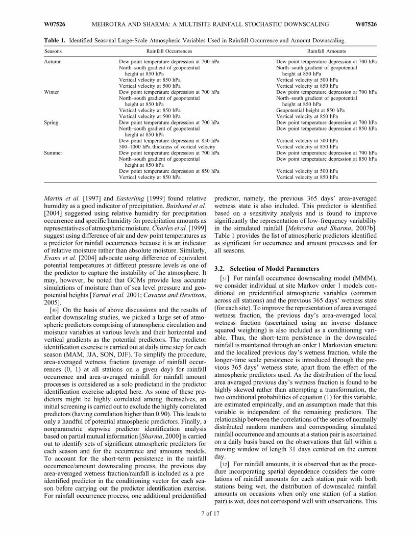
Table 1. Identified Seasonal Large‐Scale Atmospheric Variables Used in Rainfall Occurrence and Amount Downscaling

Seasons Rainfall Occurrences Rainfall Amounts

Autumn Dew point temperature depression at 700 hPa Dew point temperature depression at 700 hPaNorth–south gradient of geopotential

height at 850 hPaNorth–south gradient of geopotential

height at 850 hPaVertical velocity at 850 hPa Vertical velocity at 500 hPaVertical velocity at 500 hPa Vertical velocity at 850 hPa

Winter Dew point temperature depression at 700 hPa Dew point temperature depression at 700 hPaNorth–south gradient of geopotential

height at 850 hPaNorth–south gradient of geopotential

height at 850 hPaVertical velocity at 850 hPa Geopotential height at 850 hPaVertical velocity at 500 hPa Vertical velocity at 850 hPa

Spring Dew point temperature depression at 700 hPa Dew point temperature depression at 700 hPaNorth–south gradient of geopotential

height at 850 hPaDew point temperature depression at 850 hPa

Dew point temperature depression at 850 hPa Vertical velocity at 500 hPa500–1000 hPa thickness of vertical velocity Vertical velocity at 850 hPa

Summer Dew point temperature depression at 700 hPa Dew point temperature depression at 700 hPaNorth–south gradient of geopotential

height at 850 hPaDew point temperature depression at 850 hPa

Dew point temperature depression at 850 hPa Vertical velocity at 500 hPaVertical velocity at 850 hPa Vertical velocity at 850 hPa


7 of 17

situation occurs when a wet station lies close to the boundaryof a wet region. Neighboring dry stations tend to influencethe rainfall amount at the wet station being lesser than thevalue otherwise obtained had both stations were wet. Weaddress the influence of neighboring stations on the down-scaled rainfall amount at a station by incorporating an addi-tional variable in the predictor set, representing the ratio ofthe number of wet stations to the total number of stations inthe neighborhood (again applying a weighting factor pro-portional to the inverse interstation distance). The condition-ing vector considered for downscaling of rainfall amount ata station thus includes preidentified atmospheric variables foreach season, previous day rainfall, and a variable definingthe local wetness fraction.

4. Model Results

[33] In all the results that follow, the statistics reported areascertained by generating 100 realizations of the downscaledrainfall from the model. The individual statistics from theserealizations are ranked, and 5th, 50th, and 95th percentilevalues are extracted. The best estimate refers to the 50thpercentile value (median) while 5th and 95th percentile va-lues are used to form the confidence bands around the medianestimate. As all emission scenarios exhibit similar perfor-mances for the baseline period, results of only one emissionscenario are presented for the current climate and these arementioned hereafter as “GCM current climate.” The perfor-mance of the downscaling framework, MMM‐KDE, isevaluated on a daily, seasonal, and annual basis for its abilityto simulate various observed spatial and temporal character-istics of rainfall including those of importance in waterresource management. This assessment is performed for thebaseline period (1960–2002) during both calibration (usingreanalysis) and evaluation (using GCM current climate data)stages. In the subsequent discussions, reanalysis or GCMrainfall implies the downscaled rainfall using either reanaly-sis or GCM derived atmospheric variables. In addition tostatistics, such as means and standard deviations over definedperiods (daily, seasonal, and annual), the comparison alsoassesses various low‐frequency and extreme rainfall attri-butes such as year‐to‐year rainfall dependence attributes,number of instances when daily rainfall is greater than aprespecified threshold, extended periods of wet and dry

spells, and associated rainfall in the wet spells. Quite a fewof our results are presented in the form of contour plotsexhibiting the spatial distribution of rainfall attributes overthe study region. This is followed by the application ofdownscaling framework to simulate rainfall for year 2070using the B1, A1B, and A2 emission scenario runs and resultscompared with those for the GCM current climate and con-clusions drawn.

4.1. Model Calibration and Evaluation Overthe Baseline Period

4.1.1. Number of Wet Days and Rainfall Totals[34] For reservoir operation and flood management appli-

cations, it is important that the downscaling model accuratelyreproduces number of wet days and rainfall amounts in thedownscaled simulations. One of the strengths of the MMM‐KDE downscaling approach presented here is that the rainfalloccurrence and amounts series are simulated individually ateach station. That is, the model used for each station works inisolation, and therefore, it allows the desired properties of theindividual station rainfall to be included in the downscalingalgorithmwithout introducing additional complexities. Table 2compares the observed and downscaled (5th, median, and 95thpercentile estimates) seasonal and annual wet days and rainfalltotals over the study region. The model adequately reproducesthese rainfall occurrences and amounts attributes over the studyarea for all seasons and year during calibration (usingreanalysis data) and evaluation (using GCM current climatedata) stages. The model also captures the observed high andlow rainfall regions, for example, more wet days over theinland region in comparison to coastal during winter, morerainfall in the northern part of the region in comparisonto the southern on an annual basis, and more rainfall innorthern coastal region during summer (results not included).4.1.2. Distribution of Area‐Averaged Annual Wet Daysand Rainfall Totals[35] For efficient design and management of water

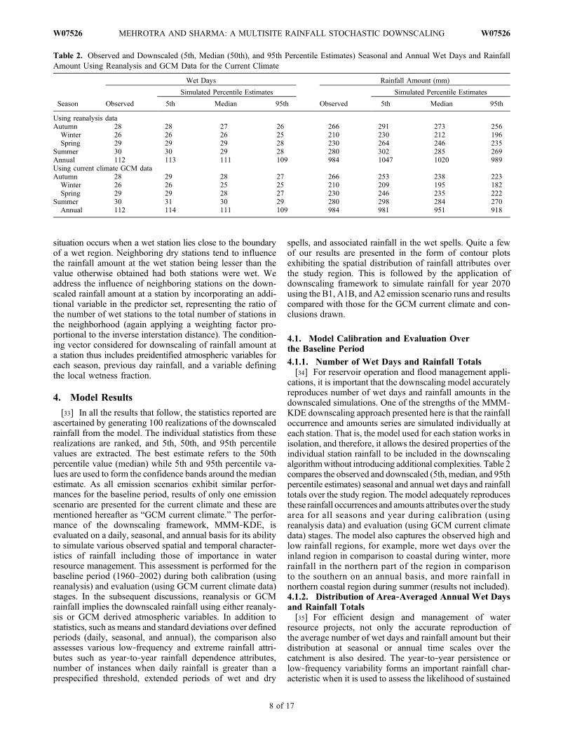
resource projects, not only the accurate reproduction ofthe average number of wet days and rainfall amount but theirdistribution at seasonal or annual time scales over thecatchment is also desired. The year‐to‐year persistence orlow‐frequency variability forms an important rainfall char-acteristic when it is used to assess the likelihood of sustained

Table 2. Observed and Downscaled (5th, Median (50th), and 95th Percentile Estimates) Seasonal and Annual Wet Days and RainfallAmount Using Reanalysis and GCM Data for the Current Climate

Season

Wet Days Rainfall Amount (mm)

Observed

Simulated Percentile Estimates

Observed

Simulated Percentile Estimates

5th Median 95th 5th Median 95th

Using reanalysis dataAutumn 28 28 27 26 266 291 273 256

Winter 26 26 26 25 210 230 212 196Spring 29 29 29 28 230 264 246 235

Summer 30 30 29 28 280 302 285 269Annual 112 113 111 109 984 1047 1020 989Using current climate GCM dataAutumn 28 29 28 27 266 253 238 223

Winter 26 26 25 25 210 209 195 182Spring 29 29 28 27 230 246 235 222

Summer 30 31 30 29 280 298 284 270Annual 112 114 111 109 984 981 951 918


8 of 17

droughts or flood regimes. Figure 2 presents the year‐to‐yeardistribution of area‐averaged wet days and rainfall amountsobtained using the reanalysis and GCM data sets. The yearlyarea‐averaged time series is formed by averaging across thestations individual station values of annual wet days andannual rainfall. Ranking of this area‐averaged series providesan indication of the over‐the‐year distribution of annualrainfall or wet days over the study region. On this figure,percentiles of the model‐simulated values are shown ascontinuous lines while the observed values are superimposedas circles. The downscaling model successfully reproducesthe distribution of observed area‐averaged annual rainfalloccurrences and amounts in the downscaled sequences, usingboth the reanalysis as well as GCM data. The good fit of thesimulated statistic indicates that the downscaling model iscapable of reproducing the observed occurrences of dry andwet years successfully over the study region. The modelperforms equally well at a majority of individual stations(results not included).4.1.3. Extreme Rainfall Characteristics[36] Sustained periods of wet and dry spells form the basis

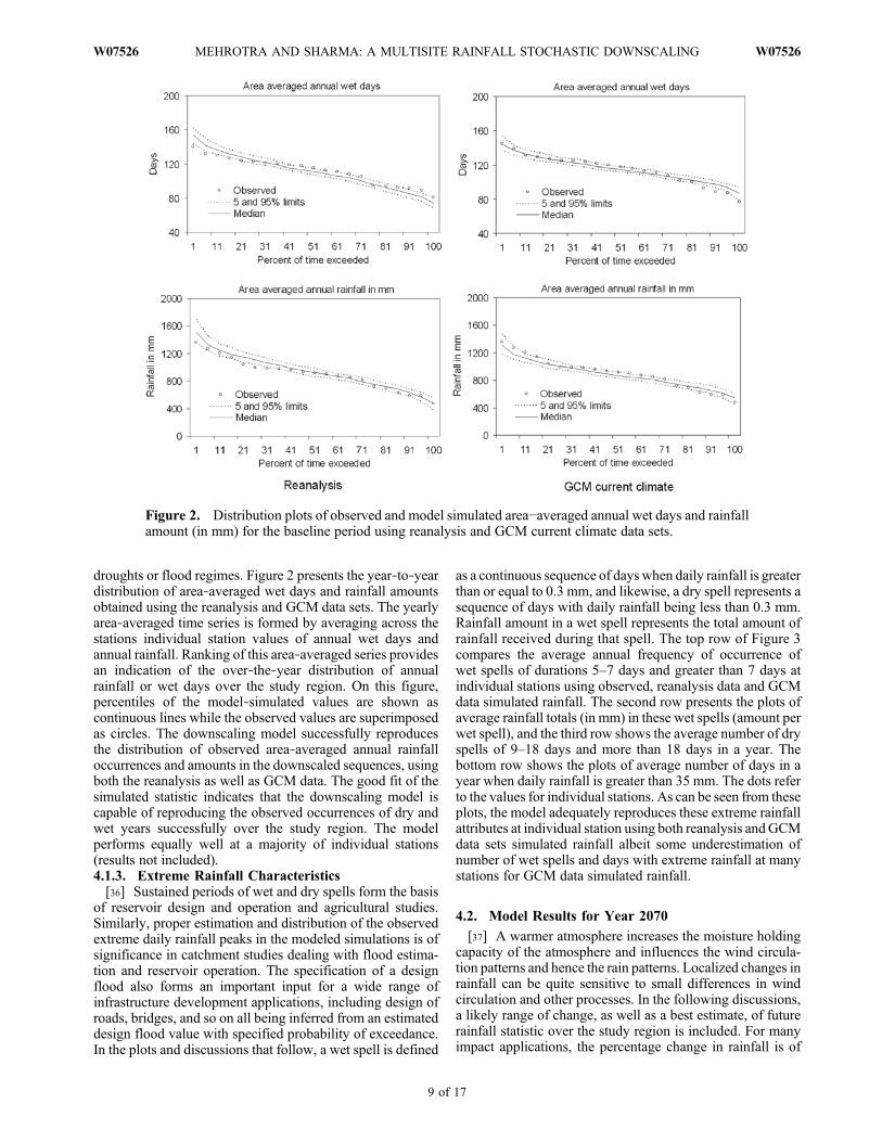
of reservoir design and operation and agricultural studies.Similarly, proper estimation and distribution of the observedextreme daily rainfall peaks in the modeled simulations is ofsignificance in catchment studies dealing with flood estima-tion and reservoir operation. The specification of a designflood also forms an important input for a wide range ofinfrastructure development applications, including design ofroads, bridges, and so on all being inferred from an estimateddesign flood value with specified probability of exceedance.In the plots and discussions that follow, a wet spell is defined

as a continuous sequence of days when daily rainfall is greaterthan or equal to 0.3 mm, and likewise, a dry spell represents asequence of days with daily rainfall being less than 0.3 mm.Rainfall amount in a wet spell represents the total amount ofrainfall received during that spell. The top row of Figure 3compares the average annual frequency of occurrence ofwet spells of durations 5–7 days and greater than 7 days atindividual stations using observed, reanalysis data and GCMdata simulated rainfall. The second row presents the plots ofaverage rainfall totals (in mm) in these wet spells (amount perwet spell), and the third row shows the average number of dryspells of 9–18 days and more than 18 days in a year. Thebottom row shows the plots of average number of days in ayear when daily rainfall is greater than 35 mm. The dots referto the values for individual stations. As can be seen from theseplots, the model adequately reproduces these extreme rainfallattributes at individual station using both reanalysis andGCMdata sets simulated rainfall albeit some underestimation ofnumber of wet spells and days with extreme rainfall at manystations for GCM data simulated rainfall.

4.2. Model Results for Year 2070

[37] A warmer atmosphere increases the moisture holdingcapacity of the atmosphere and influences the wind circula-tion patterns and hence the rain patterns. Localized changes inrainfall can be quite sensitive to small differences in windcirculation and other processes. In the following discussions,a likely range of change, as well as a best estimate, of futurerainfall statistic over the study region is included. For manyimpact applications, the percentage change in rainfall is of

Figure 2. Distribution plots of observed and model simulated area−averaged annual wet days and rainfallamount (in mm) for the baseline period using reanalysis and GCM current climate data sets.


9 of 17

Figure 3. Observed and models simulated (a) number of wet spells of 5–7 and >7 days in a year, (b) aver-age total rainfall (in mm) in these wet spells, (c) number of dry spells of 9–18 and >18 days in a year, and(d) number of days with daily rainfall >35 mm in a year.


10 of 17

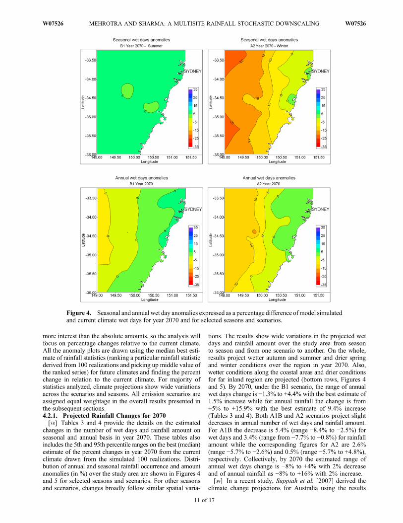
more interest than the absolute amounts, so the analysis willfocus on percentage changes relative to the current climate.All the anomaly plots are drawn using the median best esti-mate of rainfall statistics (ranking a particular rainfall statisticderived from 100 realizations and picking up middle value ofthe ranked series) for future climates and finding the percentchange in relation to the current climate. For majority ofstatistics analyzed, climate projections show wide variationsacross the scenarios and seasons. All emission scenarios areassigned equal weightage in the overall results presented inthe subsequent sections.4.2.1. Projected Rainfall Changes for 2070[38] Tables 3 and 4 provide the details on the estimated

changes in the number of wet days and rainfall amount onseasonal and annual basis in year 2070. These tables alsoincludes the 5th and 95th percentile ranges on the best (median)estimate of the percent changes in year 2070 from the currentclimate drawn from the simulated 100 realizations. Distri-bution of annual and seasonal rainfall occurrence and amountanomalies (in %) over the study area are shown in Figures 4and 5 for selected seasons and scenarios. For other seasonsand scenarios, changes broadly follow similar spatial varia-

tions. The results show wide variations in the projected wetdays and rainfall amount over the study area from seasonto season and from one scenario to another. On the whole,results project wetter autumn and summer and drier springand winter conditions over the region in year 2070. Also,wetter conditions along the coastal areas and drier conditionsfor far inland region are projected (bottom rows, Figures 4and 5). By 2070, under the B1 scenario, the range of annualwet days change is −1.3% to +4.4% with the best estimate of1.5% increase while for annual rainfall the change is from+5% to +15.9% with the best estimate of 9.4% increase(Tables 3 and 4). Both A1B and A2 scenarios project slightdecreases in annual number of wet days and rainfall amount.For A1B the decrease is 5.4% (range −8.4% to −2.5%) forwet days and 3.4% (range from −7.7% to +0.8%) for rainfallamount while the corresponding figures for A2 are 2.6%(range −5.7% to −2.6%) and 0.5% (range −5.7% to +4.8%),respectively. Collectively, by 2070 the estimated range ofannual wet days change is −8% to +4% with 2% decreaseand of annual rainfall as −8% to +16% with 2% increase.[39] In a recent study, Suppiah et al. [2007] derived the

climate change projections for Australia using the results

Figure 4. Seasonal and annual wet day anomalies expressed as a percentage difference ofmodel simulatedand current climate wet days for year 2070 and for selected seasons and scenarios.


11 of 17

from 15 best climate models simulations performed for theIPCC Fourth Assessment Report. In the study, changes inrainfall are reported for high (3.77°C by 2070), mid (2.47°Cby 2070), and low (1.17°C by 2070) global warming sce-narios, with the midscenario being close to the A2 emissionscenario. The results of the study point out increases of about10%–20% in summer and 0%–5% in autumn rainfall and

decreases of about 10% to 20% in winter and 0% to 5% inspring for midscenario. Our median estimates (Table 4,scenario A2) of 11% increase in summer, 2% increase inautumn, 9% decrease in winter, and 6% decrease in springfollow these projections fairly closely.[40] It is interesting to note that the significant increases in

the rainfall amount (25% in autumn and 16% in summer

Figure 5. Seasonal and annual rainfall anomalies expressed as a percentage difference of model simulatedand current climate rainfall for year 2070 and for selected seasons and scenarios.

Table 3. Percent Changes in Seasonal and Annual Number of Wet Days and Rainfall Amounts in 2070

Season

Current ClimateNumber ofWet Days

Scenario

B1 A1B A2

Median Estimateof Number ofWet Days

Percent Changein Median, 5th,

and 95th PercentileValues







Autumn 28 32 +13 (+18 to +9) 30 +7 (+12 to +2) 29 +3 (+7 to −2)Winter 25 23 −11 (−6 to −15) 23 −10 (−6 to −14 23 −9 (−4 to −13)Spring 28 28 −2 (+3 to −6) 26 −8 (−4 to −13) 26 −7 (−2 to −11)Summer 30 32 +6 (+11 to +2) 28 −7 (−3 to −12) 31 +3 (+7 to −1)Annual 111 113 +2 (+4 to −1) 106 −5 (−3 to −8) 109 −3 (0 to −6)

aPercent changes in number of wet days in 2070.


12 of 17

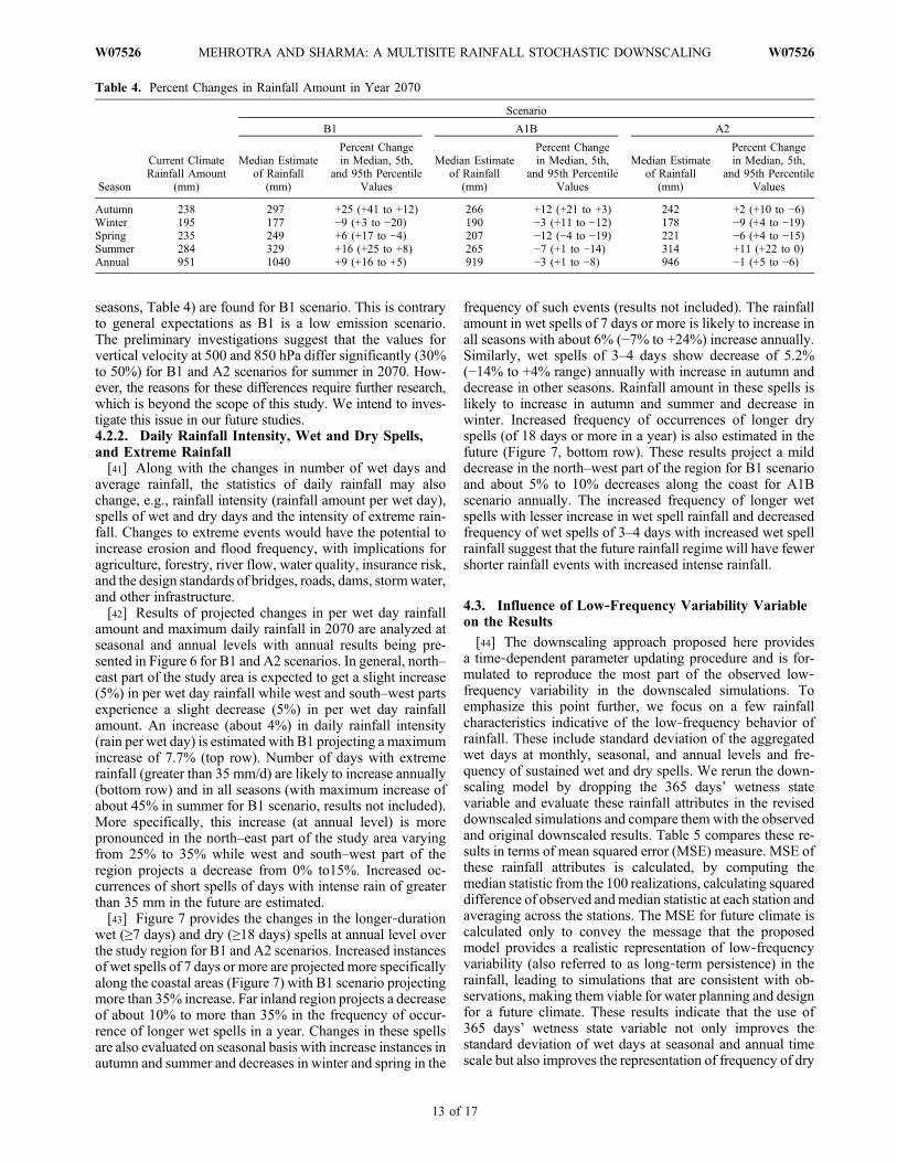
seasons, Table 4) are found for B1 scenario. This is contraryto general expectations as B1 is a low emission scenario.The preliminary investigations suggest that the values forvertical velocity at 500 and 850 hPa differ significantly (30%to 50%) for B1 and A2 scenarios for summer in 2070. How-ever, the reasons for these differences require further research,which is beyond the scope of this study. We intend to inves-tigate this issue in our future studies.4.2.2. Daily Rainfall Intensity, Wet and Dry Spells,and Extreme Rainfall[41] Along with the changes in number of wet days and

average rainfall, the statistics of daily rainfall may alsochange, e.g., rainfall intensity (rainfall amount per wet day),spells of wet and dry days and the intensity of extreme rain-fall. Changes to extreme events would have the potential toincrease erosion and flood frequency, with implications foragriculture, forestry, river flow, water quality, insurance risk,and the design standards of bridges, roads, dams, stormwater,and other infrastructure.[42] Results of projected changes in per wet day rainfall

amount and maximum daily rainfall in 2070 are analyzed atseasonal and annual levels with annual results being pre-sented in Figure 6 for B1 and A2 scenarios. In general, north–east part of the study area is expected to get a slight increase(5%) in per wet day rainfall while west and south–west partsexperience a slight decrease (5%) in per wet day rainfallamount. An increase (about 4%) in daily rainfall intensity(rain per wet day) is estimated with B1 projecting a maximumincrease of 7.7% (top row). Number of days with extremerainfall (greater than 35 mm/d) are likely to increase annually(bottom row) and in all seasons (with maximum increase ofabout 45% in summer for B1 scenario, results not included).More specifically, this increase (at annual level) is morepronounced in the north–east part of the study area varyingfrom 25% to 35% while west and south–west part of theregion projects a decrease from 0% to15%. Increased oc-currences of short spells of days with intense rain of greaterthan 35 mm in the future are estimated.[43] Figure 7 provides the changes in the longer‐duration

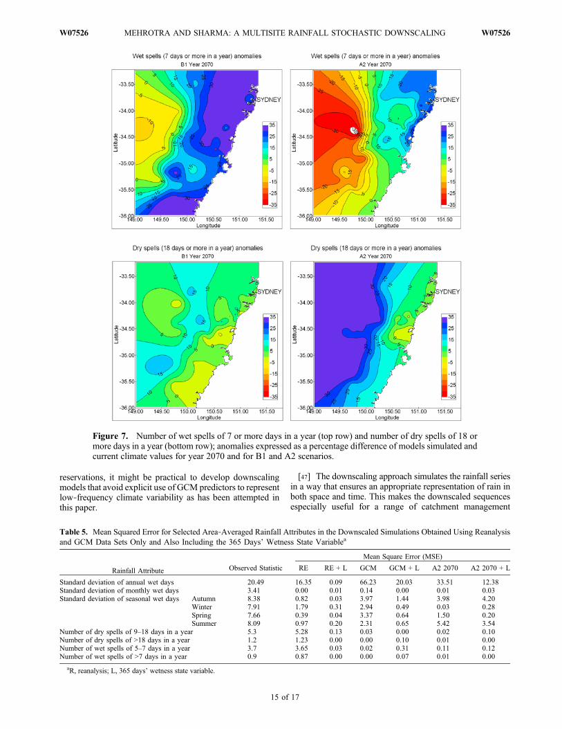
wet (≥7 days) and dry (≥18 days) spells at annual level overthe study region for B1 and A2 scenarios. Increased instancesof wet spells of 7 days or more are projected more specificallyalong the coastal areas (Figure 7) with B1 scenario projectingmore than 35% increase. Far inland region projects a decreaseof about 10% to more than 35% in the frequency of occur-rence of longer wet spells in a year. Changes in these spellsare also evaluated on seasonal basis with increase instances inautumn and summer and decreases in winter and spring in the

frequency of such events (results not included). The rainfallamount in wet spells of 7 days or more is likely to increase inall seasons with about 6% (−7% to +24%) increase annually.Similarly, wet spells of 3–4 days show decrease of 5.2%(−14% to +4% range) annually with increase in autumn anddecrease in other seasons. Rainfall amount in these spells islikely to increase in autumn and summer and decrease inwinter. Increased frequency of occurrences of longer dryspells (of 18 days or more in a year) is also estimated in thefuture (Figure 7, bottom row). These results project a milddecrease in the north–west part of the region for B1 scenarioand about 5% to 10% decreases along the coast for A1Bscenario annually. The increased frequency of longer wetspells with lesser increase in wet spell rainfall and decreasedfrequency of wet spells of 3–4 days with increased wet spellrainfall suggest that the future rainfall regime will have fewershorter rainfall events with increased intense rainfall.

4.3. Influence of Low‐Frequency Variability Variableon the Results

[44] The downscaling approach proposed here providesa time‐dependent parameter updating procedure and is for-mulated to reproduce the most part of the observed low‐frequency variability in the downscaled simulations. Toemphasize this point further, we focus on a few rainfallcharacteristics indicative of the low‐frequency behavior ofrainfall. These include standard deviation of the aggregatedwet days at monthly, seasonal, and annual levels and fre-quency of sustained wet and dry spells. We rerun the down-scaling model by dropping the 365 days’ wetness statevariable and evaluate these rainfall attributes in the reviseddownscaled simulations and compare them with the observedand original downscaled results. Table 5 compares these re-sults in terms of mean squared error (MSE) measure. MSE ofthese rainfall attributes is calculated, by computing themedian statistic from the 100 realizations, calculating squareddifference of observed andmedian statistic at each station andaveraging across the stations. The MSE for future climate iscalculated only to convey the message that the proposedmodel provides a realistic representation of low‐frequencyvariability (also referred to as long‐term persistence) in therainfall, leading to simulations that are consistent with ob-servations, making them viable for water planning and designfor a future climate. These results indicate that the use of365 days’ wetness state variable not only improves thestandard deviation of wet days at seasonal and annual timescale but also improves the representation of frequency of dry

Table 4. Percent Changes in Rainfall Amount in Year 2070

Season

Current ClimateRainfall Amount

(mm)

Scenario

B1 A1B A2

Median Estimateof Rainfall

(mm)




(mm)




(mm)



Autumn 238 297 +25 (+41 to +12) 266 +12 (+21 to +3) 242 +2 (+10 to −6)Winter 195 177 −9 (+3 to −20) 190 −3 (+11 to −12) 178 −9 (+4 to −19)Spring 235 249 +6 (+17 to −4) 207 −12 (−4 to −19) 221 −6 (+4 to −15)Summer 284 329 +16 (+25 to +8) 265 −7 (+1 to −14) 314 +11 (+22 to 0)Annual 951 1040 +9 (+16 to +5) 919 −3 (+1 to −8) 946 −1 (+5 to −6)


13 of 17

spells in the downscaled sequences specifically when usingGCM data set.

5. Summary and Conclusions

[45] This paper has demonstrated the calibration, evalua-tion, and application of a stochastic downscaling frameworkfor multisite rainfall simulation using current and futureclimate atmospheric information. The approach downscalesrainfall occurrences at multiple stations using a parametricmodified Markov model (MMM) while rainfall amounts forthe stations specified as wet on a given day by the occurrencemodel, are downscaled using conditional kernel densityestimation procedure (KDE) with spatially dependent forcingof uniform random numbers. The novelty of the downscalingapproach proposed here lies in its capability of providing atime‐dependent parameter updating procedure and reprodu-cing the observed low‐frequency variability in the down-scaled simulations. The approach modifies the day‐to‐daytransition probability of rainfall occurrences incorporatingthe changes in the values of atmospheric variables and low‐

frequency variability indicator. Similarly, rainfall amounts onthe wet days are simulated conditional on the atmosphericvariables using a nonparametric approach. Thus, the methodis capable of taking into account the variability of the climateunder the assumption that the parent distribution of atmo-spheric variables remains the same in current as well as infuture conditions. Additionally, the approach allows rainfallsimulations at individual locations independently and there-fore the restriction of spatial (in)dependence is not strictlyimposed. The only assumption involved is that given a storm,its spatial distribution across locations remains the same incurrent and future climates.[46] The selection of appropriate downscaling predictors to

represent the low‐frequency components of precipitation atpoint locations is not a straightforward task. The capabilityof GCMs to represent continental‐scale processes govern-ing low‐frequency variations in rainfall (such as El Niño–Southern Oscillation, Indian Pacific Oscillation, or similarclimatic anomalies), and the significance of future projec-tions of such mechanisms remain indecisive [e.g., Trenberthand Hoar, 1997, Wilby et al., 2002]. Acknowledging these

Figure 6. Annual “rainfall per wet day” (top row) and number of days in a year with daily rainfall greaterthan 35 mm (bottom row); anomalies expressed as a percentage difference of models simulated and currentclimate values for year 2070 and for B1 and A2 scenarios.


14 of 17

reservations, it might be practical to develop downscalingmodels that avoid explicit use of GCM predictors to representlow‐frequency climate variability as has been attempted inthis paper.

[47] The downscaling approach simulates the rainfall seriesin a way that ensures an appropriate representation of rain inboth space and time. This makes the downscaled sequencesespecially useful for a range of catchment management

Table 5. Mean Squared Error for Selected Area‐Averaged Rainfall Attributes in the Downscaled Simulations Obtained Using Reanalysisand GCM Data Sets Only and Also Including the 365 Days’ Wetness State Variablea

Rainfall Attribute Observed Statistic

Mean Square Error (MSE)

RE RE + L GCM GCM + L A2 2070 A2 2070 + L

Standard deviation of annual wet days 20.49 16.35 0.09 66.23 20.03 33.51 12.38Standard deviation of monthly wet days 3.41 0.00 0.01 0.14 0.00 0.01 0.03Standard deviation of seasonal wet days Autumn 8.38 0.82 0.03 3.97 1.44 3.98 4.20

Winter 7.91 1.79 0.31 2.94 0.49 0.03 0.28Spring 7.66 0.39 0.04 3.37 0.64 1.50 0.20Summer 8.09 0.97 0.20 2.31 0.65 5.42 3.54

Number of dry spells of 9–18 days in a year 5.3 5.28 0.13 0.03 0.00 0.02 0.10Number of dry spells of >18 days in a year 1.2 1.23 0.00 0.00 0.10 0.01 0.00Number of wet spells of 5–7 days in a year 3.7 3.65 0.03 0.02 0.31 0.11 0.12Number of wet spells of >7 days in a year 0.9 0.87 0.00 0.00 0.07 0.01 0.00

aR, reanalysis; L, 365 days’ wetness state variable.

Figure 7. Number of wet spells of 7 or more days in a year (top row) and number of dry spells of 18 ormore days in a year (bottom row); anomalies expressed as a percentage difference of models simulated andcurrent climate values for year 2070 and for B1 and A2 scenarios.


15 of 17

applications. Additionally, attributes such as the distributionof wet and dry spells, number of wet days, and rainfall amountsat individual stations have a significant impact in crop sim-ulation studies and drought management applications. Suchspatiotemporal rainfall attributes assume even more impor-tance when the downscaling procedure is applied for inves-tigating possible changes that might be experienced byhydrological, agricultural, and ecological systems in futureclimates. The substantial topographic and spatiotemporalrainfall variations of the study region provide a challengingsetting to evaluate the downscaling model.[48] The model calibration and evaluation results for the

baseline period (1960–2002) indicate that the downscalingmodel proposed here simulates fairly accurately not only thestandard rainfall attributes such as the average number of wetdays and rainfall amounts but also maximum daily rainfallamount, extended periods of wet and dry spells, and thelonger time scale variations. The scheme of updating oftransition probabilities of the at site rainfall occurrence modeland the logic of providing separate treatments for rainfalloccurrence and amounts at individual locations, providesconsiderable improvements in the representation of char-acteristics of interest in hydrologic studies for current andfuture climates and therefore offers a convenient tool for usein climate change impact assessment studies.[49] The utility of the proposed downscaling framework is

subsequently demonstrated by estimating the plausiblechanges in rainfall in year 2070. Downscaled results for 2070show variations across the seasons and emission scenarios. Ingeneral, wetter autumn and summer and drier winter andspring with coastal region getting wetter and inland regionbecoming drier are estimated. Increased instances of longerdry and wet spells with lighter rain are expected to occur inthe future.[50] The present study makes use of three emission sce-

narios runs simulated using a single GCM (CSIRO Mk3.0)only. While this not the main focus of the paper, this rep-resents a limitation of the work presented here. Use of addi-tional GCMs with multiple ensemble members are likely tocontribute to a more appropriate reflection of the uncertaintyassociated with the rainfall projections for the future. Itshould, however, be noted, that while there are significantinconsistencies across GCMs in their simulation of variablessuch as rainfall or flow for a future climate, these incon-sistencies are generally lower for the atmospheric predictorsthe downscaling application has utilized. For instance, in astudy across Australia, Johnson and Sharma [2009] report avariable convergence score having a range of 0 to 100 (with100 representing uniformity in GCM simulations for a futureclimate for the variable), which associates high skills formonthly simulations of the predictors that have been usedin the downscaling model (averaged skills for the grid celllocations used in the downscaling model for surface pressure,geopotential heights (700 hPa) and dew point temperaturedepression (700 hPa) being 97, 89, and 53, respectively, incontrast to precipitation, which has a skill of 14. Skill scoresfor vertical velocity are not available. Consequently, we arguethat if downscaling models are formulated using predictorsthat are deemed to be more skillful across GCMs in their si-mulations for a future climate, the consequences of usingfewer GCMs in a downscaling assessment are likely to belower.

[51] Acknowledgments. The work described in this paper is partiallyfunded by the Australian Research Council, Sydney Catchment Authorityand Department of Environment, Climate Change and Water, New SouthWales, Australia. We are also thankful to three anonymous referees for theirconstructive comments.

ReferencesBartholy, J., I. Bogardi, and I. Matyasovszky (1995), Effect of climatechange on regional precipitation in lake Balaton watershed, Theor Appl.Climatol., 51, 237–250.

Benestad, R. E. (2001), The cause of warming over Norway in theECHAM4/OPYC3 GHG integration, Int. J. Climatol., 21, 1645–1668.

Bergstrom, S., B. Carlsson, M. Gardelin, G. Lindstrom, A. Pettersson,and M. Rummukainen, (2001), Climate change impacts on runoff inSweden—assessments by global climate models, dynamical downscalingand hydrological modeling, Clim. Res., 16, 101–112.

Buishand, T. A., M. V. Shabalova, and T. Brandsma (2004), On the choiceof the temporal aggregation level for statistical downscaling of precipita-tion, J. Clim., 17(9), 1816–1827.

Burger, G. (1996), Expanded downscaling for generating local weatherscenarios, Clim. Res., 7, 111–128.

Burger, G., and Y. Chen (2005), Regression‐based downscaling of spatialvariability for hydrologic applications, J. Hydrol., 311, 299–317.

Cavazos, T. (1997), Downscaling large‐scale circulation to local winterrainfall in N.E. Mexico, Int. J. Climatol., 17, 1069–1082.

Cavazos, T., and B. C. Hewitson (2005), Performance of NCEP‐NCARreanalysis variables in statistical downscaling of daily precipitation,Clim. Res., 28, 95–107.

Charles, S. P., B. C. Bates, and J. P. Hughes (1999), A spatiotemporalmodel for downscaling precipitation occurrence and amounts, J. Geophys.Res., 104(D24), 31,657–31,669.

Charles, S. P., B. C. Bates, I. N. Smith, and J. P. Hughes (2004), Statisticaldownscaling of daily precipitation from observed and modeled atmosphericfields, Hydrol. Processes, 18, 1373–1394.

Christensen, J. H., T. R. Carter, M. Rummukainen, and G. Amanatidis(2007), Evaluating the performance and utility of regional climate mod-els: the PRUDENCE project, Clim. Change, 81(Suppl.), 1–6.

Dehn, M., G. Bürger, J. Buma, and P. Gasparetto (2000), Impact of climatechange on slope stability using expanded downscaling, Eng. Geol., 55,193–204.

Easterling, D. (1999), Development of regional climate change scenariosusing a downscaling approach, Clim. Change, 41, 615–634.

Evans, J. P., B. S. Ronald, and J. O. Robert (2004), Middle east climatesimulation and dominant precipitation processes, Int. J. Climatol., 24,1671–1694.

Fowler, H. J., M. Ekström, C. G. Kilsby, and P. D. Jones (2005), Newestimates of future changes in extreme rainfall across the UK usingregional climate model integrations: 1. Assessment of control climate,J. Hydrol., 300, 212–233.

Fowler, H. J., S. Blenkinsop, and C. Tebaldi (2007), Linking climatechange modeling to impacts studies: recent advances in downscalingtechniques for hydrological modeling, Int. J. Climatol., 27(12), 1547–1578.

Frei, C., R. Schöll, S. Fukutome, J. Schmidli, and P. L. Vidale (2006),Future change of precipitation extremes in Europe: an intercomparisonof scenarios from regional climate models, J. Geophys. Res., 111,D06105, doi:10.1029/2005JD005965.

Giorgi, F., B. Hewitson, J. Christensen, M. Hulme, H. Von Storch,P.Whetton, R. Jones, L.Mearns, andC. Fu (2001), Regional climate infor-mation: evaluation and projections (chapter 10), in Climate Change 2001:The Scientific Basis, Contribution of Working Group I to the Third Assess-ment Report of the IPCC, edited by J. T. Houghton et al., pp. 739–768,Cambridge Univ. Press, Cambridge.

Gordon, H. B., et al. (2002), The CSIRO Mk3 Climate System Model(Electronic publication). Aspendale: CSIRO Atmospheric Research.(CSIRO Atmospheric Research technical paper, no. 60), 130 pp.(http://www.dar.csiro.au/publications/gordon_2002a.pdf).

Hanssen‐Bauer, I., and E. J. Forland (2000), Temperature and precipitationvariations in Norway 1900–1994 and their links to atmospheric circula-tion, Int. J. Climatol., 20(14), 1963–1708.

Harpham, C., and R. L. Wilby (2005), Multi‐site downscaling of heavydaily precipitation occurrence and amounts, J. Hydrol., 312, 1–21.

Harrold, T. I., A. Sharma, and S. J. Sheather (2003), A nonparametricmodel for stochastic generation of daily rainfall occurrence, WaterResour. Res., 39(12), 1343, doi:10.1029/2003WR002570.


16 of 17

Hennessy, K., et al. (2008), An assessment of the impact of climate changeon the nature and frequency of exceptional climatic events, report,CSIRO and the Bureau of Meteorology to the Australian Govern-ment. Commonwealth of Australia, Canberra, (http://www.daff.gov.au/agriculture‐food/drought/national_review_of_drought_policy/climatic_assessment).

Hewitson, B. C., and R. G. Crane (1996), Climate downscaling: techniquesand application, Clim. Res., 7, 85–95.

Hughes, J. P., and P. Guttorp (1994), A class of stochastic models for relat-ing synoptic atmospheric patterns to regional hydrologic phenomena,Water Resour. Res., 30, 1535–1546.

Hughes, J. P., P. Guttorp and S. P. Charles (1999), A non‐homogeneoushidden Markov model for precipitation occurrence, Appl. Stat., 48(1),15–30.

Huth, R. (1999), Statistical downscaling in central Europe: evaluation ofmethods and potential predictors, Clim. Res., 13, 91–101.

Ines, A. V. M. and J. W. Hansen (2006), Bias correction of daily GCMrainfall for crop simulation studies, Agricultural and Forest Meteorol-ogy, 138(1–4), 44–53.

IPCC (2007), Climate Change 2007: The Physical Science Basis. Contribu-tion of Working Group I to the Fourth Assessment Report of the Inter-governmental Panel on Climate Change, edited by S. Solomon et al.,Cambridge Univ. Press, Cambridge, United Kingdom and New York,NY, USA.

Johnson, F. and A. Sharma (2009), Measurement of GCM skill in predict-ing variables relevant for hydroclimatological assessments, J. Clim.,22(16), 4373–4382.

Karl, T. R., W. C. Wang, M. E. Schlesinger, R. W. Knight, and D. Portman(1990), A method of relating general circulation model simulated climateto observed local climate, Part I: seasonal statistics, J. Clim., 3, 1053–1079.

Katz, R. W., and M. B. Parlange (1993), Effects of an index of atmosphericcirculation on stochastic properties of precipitation, Water. Resour. Res.,29, 2335–2344.

Katz, R. W., and M. B. Parlange (1996), Mixtures of stochastic processes:application to statistical downscaling, Clim. Res., 7, 185–193.

Kiely, G., J. D. Albertson, M. B. Parlange, and R. W. Katz (1998), Condi-tioning stochastic properties of daily precipitation on indices of atmo-spheric circulation, Meteorol. Appl., 5, 75–87.

Knutti, R. (2008), Should we believe model predictions of future climatechange?, Philos. Trans. R. Soc. London, Ser. A, 366(1885), 4647–4664.

Kyselý, J. (2002), Comparison of extremes in GCM‐simulated, downscaledand observed central‐European temperature series, Clim. Res., 20, 211–222.

Martin, E., B. Timbal and E. Brun, (1997), Downscaling of general circu-lation model outputs: simulation of the snow climatology of the FrenchAlps and sensitivity to climate change, Clim. Dyn., 13, 45–56.

Mearns, L. O., M. Hulme, T. R. Carter, R. Leemans, M. Lal, and P. Whetton,(2001), Climate Scenario Development (Chapter 13), in Climate Change2001: The Scientific Basis, 36 Contribution of Working Group I to theThird Assessment Report of the IPCC, edited by J. T. Houghton,pp. 583–638, Cambridge Univ. Press, Cambridge.

Mearns, L. O., F. Giorgi, P. Whetton, D. Pabon, M. Hulme, and M. Lal(2004), Guidelines for use of climate scenarios developed from regionalclimate model experiments, Tech. Rep., Data Distribution Center of theIPCC.

Mehrotra, R. and A. Sharma (2005), A nonparametric nonhomogeneoushidden Markov model for downscaling of multi‐site daily rainfall occur-rences, J. Geophys. Res., 110, D16108, doi:10.1029/2004JD005677.

Mehrotra, R., and A. Sharma (2007a), A semi‐parametric model for sto-chastic generation of multi‐site daily rainfall exhibiting low frequencyvariability, J. Hydrol., 335, 180–193, doi:10.1016/j.jhydrol.2006.11.011.

Mehrotra, R., and A. Sharma (2007b), Preserving low‐frequency variabilityin generated daily rainfall sequences, J. Hydrol., 345, 102–120,doi:10.1016/j.jhydrol.2007.08.003.

Mehrotra, R., A. Sharma, and I. Cordery (2004), Comparison of twoapproaches for downscaling synoptic atmospheric patterns to multisiteprecipitation occurrence, J. Geophys. Res., 109, D14107, doi:10.1029/2004JD004823.

Mehrotra, R., R. Srikanthan, and A. Sharma (2006), A comparison of threestochastic multi‐site precipitation occurrence generators, J. Hydrol., 331,280–292, doi:10.1016/j.jhydrol.2006.05.016.

Micevski, T., S. Franks, and G. Kuczera (2006), Multidecadal variability incoastal eastern Australian flood data, J. Hydrol., 327, 219–225.

Milly, P. C. D., J. Betancourt, M. Falkenmark, R. M. Hirsch, Z. W.Kundzewicz, D. P. Lettenmeier, and R. J. Stouffer (2008), Climatechange—stationarity is dead: Whither water management?, Science,319(5863), 573–574.

Muller‐Wohlfeil, D. I., G. Bürger, and W. Lahmer (2000), Response of ariver catchment to climate change: application of expanded downscalingto northern Germany, Clim. Change, 47, 61–89.

Schmidli, J., C. M. Goodess, C. Frei, M. R. Haylock, Y. Hundecha,J. Ribalaygua, and T. Schmith (2007), Statistical and dynamical down-scaling of precipitation: An evaluation and comparison of scenarios forthe European Alps, J. Geophys. Res., 112, D04105, doi:10.1029/2005JD007026.

Scott, D. W. (1992), Multivariate density estimation: Theory, practice andvisualization, John Wiley, New York.

Sharma, A. (2000), Seasonal to interannual rainfall probabilistic forecastsfor improved water supply management: Part 3—A nonparametric prob-abilistic forecast model, J. Hydrol., 239, 249–258.

Sharma, A., and R. O’Neill (2002), A nonparametric approach for repre-senting interannual dependence in monthly streamflow sequences, WaterResour. Res., 38(7), 1000, doi:10.1029/2001WR000953.

Stehlík, J., and A. Bárdossy (2002), Multivariate stochastic downscalingmodel for generating daily precipitation series based on atmosphericcirculation, J. Hydrol., 256, 120–14.

Suppiah, R., K. J. Hennessy, P. H. Whetton, K. McInnes, I. Macadam,J. Bathols, J. Ricketts, and C. M. Page, 2007, Australian climate changeprojections derived from simulations performed for the IPCC 4th Assess-ment Report, Aust. Meterol. Mag., 56, 131–152.

Trenberth, K. E., and T. J. Hoar (1997), El Nino and climate change,Geophys. Res. Lett., 24, 3057–3060.

Trenberth, K. E., A. Dai, R. M. Rasmussen, and D. B. Parsons (2003), Thechanging character of precipitation, Bull. Am. Meteorol. Soc., 1205–1217, doi:10.1175/BAMS-84-9-1205.

Varis, O., T. Kajander, and R. Lemmelä (2004), Climate and water: fromclimate models to water resources management and vice versa, Clim.Change, 66, 321–344.

Vicuna, S., P. E. Murer, B. Joyce, J. A. Dracup, and D. Purkey (2007), Thesensitivity of California water resources to climate change scenarios,Water Resour. Assoc., 43, 482–499.

von Storch, H. (1999), On the Use of “Inflation” in Statistical Downscaling,J. Clim., 12, 3505–3506.

Vrac, M., and P. Naveau (2007), Stochastic downscaling of precipitation:from dry to heavy rainfalls, Water Resour. Res., 43, W07402,doi:10.1029/2006WR005308.

Wang, Y. P., and D. J. Connor (1996), Simulation of optimal developmentfor spring wheat at two locations in southern Australia under present andchanged climate conditions, Agr. Forest Meteorol., 79, 9–28.

Wilby, R. L. (1998), Statistical downscaling of daily precipitation usingdaily airflow and seasonal teleconnection indices,Clim. Res., 10, 163–178.

Wilby, R. L., and T. M. L. Wigley (1997), Downscaling general circulationmodel output: a review of methods and limitations, Prog. Phys. Geogr.,21, 530–548.

Wilby, R. L., D. Conway, and P. D. Jones (2002), Prospects for downscal-ing seasonal precipitation variability using conditioned weather generatorparameters, Hydrol. Process., 16, 1215–1234.

Wilby, R. L., S. P. Charles, E. Zorita, B. Timbal, P. Whetton, and L. O.Mearns (2004), Guidelines for use of climate scenarios developed fromstatistical downscaling methods, Tech. Rep., Data Distribution Center ofthe IPCC.

Wilks, D. S. (1998), Multisite generalization of a daily stochastic precipi-tation generation model, J. Hydrol., 210, 178–191.

Woodhouse, C. A. (1997), Winter climate and atmospheric circulation pat-terns in the Sonoran desert region, USA, Int. J. Climatol., 17, 859–873.

Woolhiser, D. A., T. O. Keefer, and K. T. Redmond (1993), SouthernOscillation effects on daily precipitation in the southwestern UnitedStates, Water Resour. Res., 29, 1287–1295.

Yarnal, B., A. C. Comrie, B. Frakes, and D. P. Brown (2001), Develop-ments and prospects in synoptic climatology, Int. J. Climatol., 21,1923–1950.

R. Mehrotra and A. Sharma, Water Research Center, School of Civil andEnvironmental Engineering, University of New South Wales, Sydney,NSW 2052, Australia. ([email protected])


17 of 17

Development and application of a multisite rainfall stochastic downscaling framework for climate...

Documents

Transcript of Development and application of a multisite rainfall stochastic downscaling framework for climate...