HAL Id: hal-00831459https://hal.archives-ouvertes.fr/hal-00831459

Submitted on 7 Jun 2013

HAL is a multi-disciplinary open accessarchive for the deposit and dissemination of sci-entific research documents, whether they are pub-lished or not. The documents may come fromteaching and research institutions in France orabroad, or from public or private research centers.

L’archive ouverte pluridisciplinaire HAL, estdestinée au dépôt et à la diffusion de documentsscientifiques de niveau recherche, publiés ou non,émanant des établissements d’enseignement et derecherche français ou étrangers, des laboratoirespublics ou privés.

Robust formation-tracking control of mobile robots in aspanning-tree topologyJanset Dasdemir, Antonio Loria

To cite this version:Janset Dasdemir, Antonio Loria. Robust formation-tracking control of mobile robots in a spanning-tree topology. International Journal of Control, Taylor & Francis, 2014, 87 (9), pp.1822-1832. �hal-00831459�

Robust formation-tracking control of mobile

robots in a spanning-tree topology

Janset Dasdemira and Antonio Loriab∗

aYildiz Technical University, TurkeybCNRS, L2S-Supelec, 3 Rue Joliot Curie, Gif sur Yvette France.

Abstract. We solve the formation-tracking control problem for mobile robots via linear control, under theassumption that each agent communicates only with one “leader” robot and with one follower. As in the classicaltracking control problem for nonholonomic systems, the swarm is driven by a fictitious robot which moves aboutfreely and which is leader to one robot only. For a spanning-tree topology we show that persistency of excitationon the velocity of the virtual leader is sufficient and necessary to achieve consensus tracking. Furthermore, weestablish uniform global exponential stability for the error system which implies robustness with respect toadditive bounded disturbances. From a graph viewpoint, our main result corroborates that the existence of aspanning tree is necessary and sufficient for consensus as opposed to the usual but restrictive assumption ofall-to-all undirected communication.

Keywords: Mobile robots, formation control, tracking control, consensus.

1 Introduction

It is clear in a vast number of scenarios that a group of robots may accomplish certain tasks withgreater efficiency, flexibility, robustness and safety than a single robot. However, coordinatedmotion requires in general more complex control schemes as well as path planning. For instance,it may be achieved through local individual tracking control on each robot provided that allagents communicate with each other; this is an assumption commonly made in the literature.Furthermore, in many applications such as search & rescue, surveillance or transportation, agroup of mobile robots is supposed to follow a predefined trajectory while maintaining a desiredformation shape. It is also often assumed that all robots in the swarm know the reference tra-jectory. Under such circumstances, the problem of formation control ressembles that of trackingcontrol repeated for each individual. Beyond the particular problem of trajectory tracking thereare a number of challenging problems such as path-planning and path-following, fault detection,obstacle avoidance, etc. In this paper we focuss on formation tracking control.

There are various formation-control methods proposed in the literature. According to the be-havior approach of Balch and Arkin (1998), Lawton et al. (2003), desired behaviors such asobstacle avoidance or target seeking, are assigned to each vehicle and formation control action isdetermined by a weighted average of all desired behaviors. This approach is useful when agentshave multiple competing objectives however, it typically relies on an all-to-all communicationamong agents and from an analysis viewpoint, it is generally mathematically complex. Followingthe virtual structure method Lewis and Tan (1997), Yoshioko and Namerikawa (2008) the entireformation is treated as a single body which can evolve in a given direction and orientation tobuild a predefined time-invariant formation shape. Although it is rather easy to prescribe thecoordinated behavior and it has certain robustness to perturbations on robots, trajectories aregenerated in a centralized fashion leading to a virtual rigid structure; this may result in a pointof failure for the whole swarm of agents. In the recent article Sadowska et al. (2011), so-called

∗Corresponding author. E-mail: loria@lss.supelec.fr

1

mutual coupling terms are added to the controller to cope with tracking and time-varying forma-tions under perturbations however, the desired trajectories of each robot depend on the trajectoryof the virtual structure and it relies on the assumption that the topology graph is undirectedand may present communication constraints. The graph-theory approach as in Fax and Murray(2004), Olfati-Saber and Murray (2002), Ren and Sorensen (2008) relies on the definition ofLaplacian matrices to describe communication links and stability of the system is ensured bystability of each individual system and the connectivity of the graph. It is important to mentionthat the papers mentioned above are restricted to linear systems. On the other hand, in Donget al. (2006) the graph theory approach is used in order to design controller for nonholonomicmobile agents.

The leader-follower approach as in Desai et al. (2001), Fierro et al. (2001) is reminiscent ofmaster-slave synchronization. Extended to the case of more than two agents, one or more vehiclesmay be considered as leader and the rest of the robots are considered followers as they are requiredto track their leaders’ trajectories with a predefined formation shape. In the context of mobilerobots, a virtual reference vehicle is assumed as a leader over all the rest. From a graph viewpoint,it is the reference vehicle which plays the role of a root node. Leaders are children of the rootnode that is, robots which “know” the reference trajectory. All other nodes are either followersand leaders simultaneously (intermediate nodes in the graph topology) or they are followers(leaves, nodes without children in the graph topology). Besides being easy to understand and toimplement, the method is scalable for any number of agents. There is no explicit feedback fromfollowers to leaders (the graph is directed) but followers require full state information of theirleaders.

In Guo et al. (2010), an adaptive leader-follower based formation control without the need ofleaders’ velocity information is proposed. It is assumed that two robots act as leaders hence, theyknow the prescribed reference velocity, while the others are considered to be followers, with singleintegrator dynamics. A stability analysis shows that the triangular formation is asymptoticallystable while the co-linear one is not. In Shao et al. (2007), the authors present a three-levelhybrid control architecture based on feedback linearization; the analysis relies on graph theory.It shows that position error system is asymptotically stable with a bounded orientation error. InGhommam et al. (2011), a virtual vehicle is designed to eliminate velocity measurement of theleader then using backstepping and Lyapunov’s direct method position tracking control problemof the follower is solved. The proposed method guarantees asymptotic stability of the closed looperror system dynamic. Another asymptotic stability result is presented in Consolini et al. (2008).The proposed control strategy ensures the follower position to vary in proper circle arcs centeredat the leader’s reference frame, satisfying suitable input constraints.

In Soorki et al. (2011) and LIU et al. (2007), feedback linearization and sliding-mode-basedcontrol is employed for two robots in a leader-follower formation. They exhibit robustness tobounded disturbances and unmodeled dynamics with asymptotically stable closed-loop system.In Sira-Ramírez and Castro-Linares (2010), the leader’s influence on the trajectory tracking errordynamics is taken as an unknown but bounded, observable disturbance and eliminated by thelocal controllers of followers. Trajectory errors asymptotically converge to a small vicinity of theorigin. In the presence of unknown internal dynamics, an optimal formation control problem issolved in Dierks et al. (2012). Using adaptive dynamic programming with NN, it is showed thatthe kinematic tracking error, the velocity tracking error and the parameter estimation errorsare all uniformly ultimately bounded. In Gamage et al. (2010), three different formation controlmethods are addressed. Two of them are solved by using virtual robot path tracking techniques,one of which is based on approximate linearization of the unicycle dynamics and the other isformed using Lyapunov-based nonlinear time varying design. The third controller is developedthrough dynamic feedback linearization. A comparative study by means of stability and forma-tion success of the proposed methods and an existing fourth static feedback linearization basedformation controller is presented. In ZHANG (2010), consensus protocols under directed com-munication topology are designed using time-varying consensus gains to reduce the noise effects.

2

Asymptotic mean square convergence of the tracking errors is provided through algebraic graphtheory and stochastic analysis.

In this paper, we follow a leader-follower approach; we assume that the swarm of n vehicleshas only one leader which communicates with the virtual reference vehicle that is, only one robotknows the reference trajectory. The formation is ensured via a one-to-one unilateral communi-cation that is, each robot except for the leader (root agent) and the last follower (tail agent),communicates only with one follower and with one leader. To the former the robot gives informa-tion of its full state, from the latter it receives full state information which is taken by the localcontroller as a reference. The communication graph is directed that is, there exist no feedbackfrom followers to leaders. We solve the problem for both models available in the literature: thevelociy-controlled kinematics-only model and the force-controlled dynamic model (with an addedintegrator).

Our controllers are inspired by similar controllers previously reported for tracking control ofa single robot. The control design and therefore the stability analysis problems, are dividedinto the tracking control for the translation variables and tracking of the heading angle. Thisseparation-principle approach leads to fairly simple controllers, linear time-varying. The analysisrelies on the ability to study the behavior of the translational errors and heading errors separately.For the former, it is established that a sufficient and necessary condition is that the referenceangular trajectory of the virtual leader robot have the property of persistency of excitation, forthe heading angles, a simple proportional feedback is enough. The analysis of the over-all closedloop system relies on tracking theorems tailored for so-called cascaded (time-varying) systems.The significance of the proof method relies in the circumvention of graph theory, eigen-valueanalysis and other tools difficult to extend to the realm of nonlinear systems. This makes ourmethod particularly fitted for non-trivial extensions such as to the case of time-varying and state-dependent interconnections (for instance, in the case that the dynamics of the communicationchannel is considered).

The rest of the paper is organized as follows. In Section 2 we recall the kinematic model of themobile robot and formulate the formation tracking control problem. In Section 3, we present ourmain results. In Section 4 we present some illustrative simulation results and we conclude withsome remarks in Section 5.

2 Problem formulation and its solution

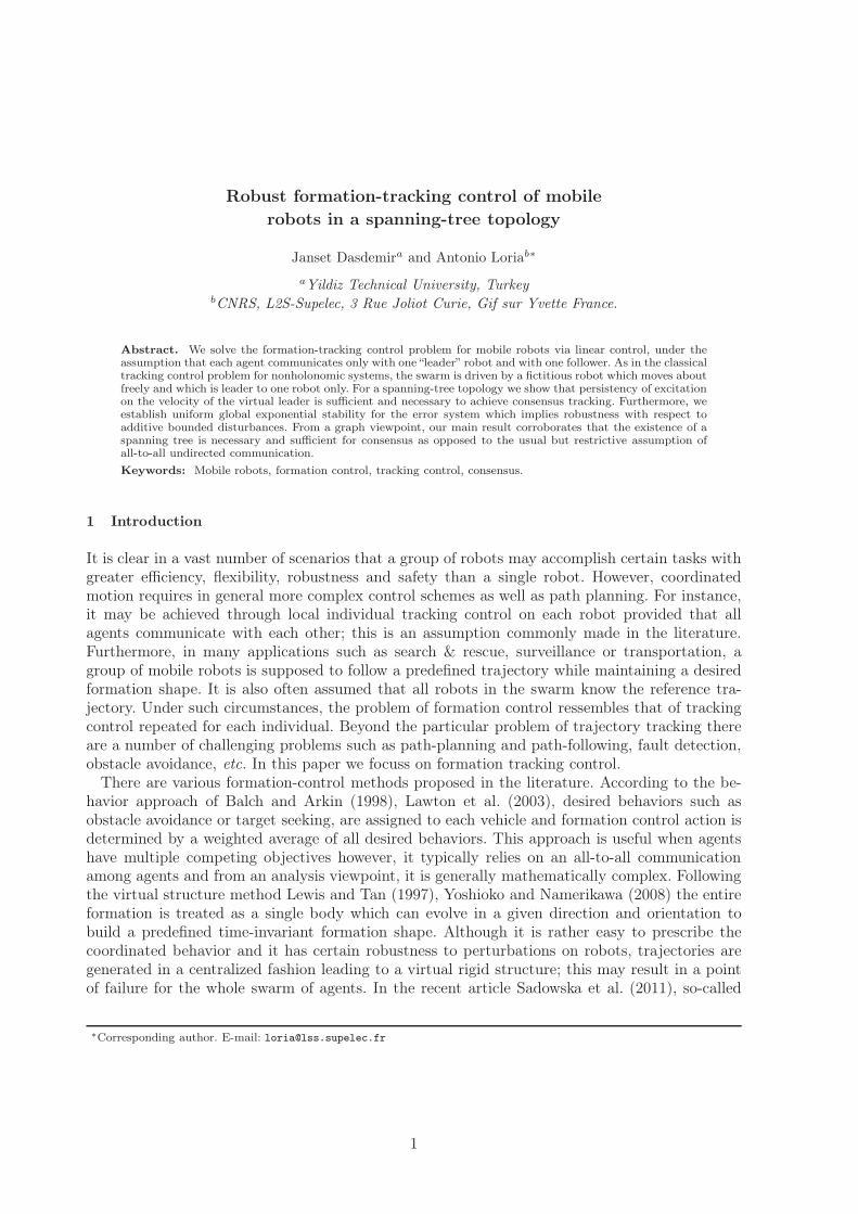
Figure 1. Generic representation of a leader-follower configuration. For a swarm of n vehicles, any geometric topology maybe easily defined by determining the position of each vehicle relative to its leader. This does not affect the kinematic model.

3

Consider a group of n mobile robots, whose kinematic models are given by

xi = vi cos (θi) (1a)

yi = vi sin (θi) (1b)

θi = wi, i ∈ [1, n] (1c)

where the coordinates xi and yi represent the center of the i th mobile robot with respect toa globally-fixed frame and θi is the heading angle –see Figure 1 and the linear and angularvelocities of the i th robot are denoted respectively vi and wi. In the case that each vehicle isvelocity-controlled the decentralized control inputs are vi and wi.

The control objective is to make the n robots take specific postures determined by the topologydesigner, and to make the swarm follow a path determined by a virtual reference vehicle labeledR0. Any physically feasible geometrical configuration may be achieved and one can choose anypoint in the Cartesian plane to follow the virtual reference vehicle. The swarm has only one‘leader’ robot tagged R1 whose local controller uses knowledge of the reference trajectory gener-ated by the virtual leader; in the communications graph, R1 is the child of the root-node robotR0. The other robots are intermediate robots labeled R2 to Rn−1 that is, Ri acts as leader forRi+1 and follows Ri−1. The last robot in the communication topology is denoted Rn and hasno followers that is, it constitutes the tail node of the spanning tree –see Figure 2. We remarkthat the notation Ri−1 refers to the graph topology as illustrated in Figure 2 but it does notdetermine a physical formation.

Figure 2. Communication topology: a spanning directed tree with permanent communication between Ri and Ri+1 forall i ∈ [0, n− 1] .

The reference vehicle describes the reference trajectory defined by

x0 = v0 cos (θ0)

y0 = v0 sin (θ0)

θ0 = w0

that is, v0 and w0 are respectively, the desired linear and angular velocities communicated to theleader robot R1 only.

After the seminal paper Kanayama et al. (1990) we introduce error variables to denote thedifference between the leader and follower states, in the present context these are the virtualreference vehicle R0 and the swarm leader R1, then

p1x = x0 − x1

p1y = y0 − y1

p1θ = θ0 − θ1.

Next, we transform the error coordinates [p1x, p1y, p1θ] of the leader robot from the global

4

coordinate frame to local coordinates fixed on the robot that is,

e1xe1ye1θ

=

cos θ1 sin θ1 0− sin θ1 cos θ1 0

0 0 1

p1xp1yp1θ

. (2)

In the new coordinates, the error dynamics between the reference vehicle and the leader of theswarm becomes

e1x = w1e1y − v1 + v0 cos e1θ (3a)

e1y = −w1e1x + v0 sin e1θ (3b)

e1θ = w0 − w1 (3c)

and we proceed with the obvious modifications to express the “tracking” errors between anyleader-follower couple of robots. Therefore, we may approach the formation control problemunder a spanning-tree topology as a sequential leader-follower tracking problem. As it is observedin a large body of literature that followed Kanayama et al. (1990), the leader-follower trackingcontrol problem boils down to the stabilization of the origin of (3) –see e.g. Lefeber (2000) andthe references therein.

In Panteley et al. (1998) cascaded-based control is used to design linear controllers that stabilizethe origin of (3); tools from linear adaptive control systems theory are used to establish stability.In this paper we extend this approach to the case of formation tracking control of several mobilerobots interacting as it is explained above. Before presenting our main results it is convenient toexplain the rationale of the control design and stability analysis methods that we employ.

2.1 Cascaded-based tracking control

Cascaded-based control relies on the ability to design controllers so that the closed-loop systemhas a cascaded structure,

x1 = f1 (t, x1) + g (t, x) (4a)

x2 = f2 (t, x2) (4b)

where x1 ∈ Rn1 , x2 ∈ R

n2 . Note that the lower dynamics (4b) is independent of the variable x1and the dynamic equation corresponding to the latter is “perturbed” by x2 through the intercon-nection term g (t, x), hence the term cascade. Stability of the origin of the cascaded system maybe asserted by relying on (Panteley and Loría 2001, Lemma 3), which establishes that the originof a cascaded system is uniformly globally asymptotically stable if so are the respective origins ofthe disconnected subsystems that is, when the interconnection g ≡ 0 and if the solutions of theperturbed dynamics (7) remain bounded. In the appendix we present a concrete stability theoremwhose conditions serve as guidelines for control design and fits the purposes of this paper.

In that regard, it is important to stress that the error dynamics (3) already possesses a cascadedstructure, with x2 = e1θ; indeed, the latter may be regarded as an input generating a perturbationto the translational dynamics equations (3a), (3b). With this in mind, we follow the approachoriginally proposed in Panteley et al. (1998), where uniform global exponential stability wasfirst established for the tracking control problem with linear control and under persistency of

5

excitation conditions1. Define

v1 = v0(t) + c2e1x (5a)

w1 = w0(t) + c1e1θ (5b)

then, the closed loop error dynamics can be obtained as follows

e1x = [w0e1y − c2e1x] + [c1e1θe1y+v0(cos e1θ − 1)] (6a)

e1y = [−w0e1x] + [−c1e1θe1x + v0 sin e1θ] (6b)

e1θ = −c1e1θ. (6c)

Note that the third equation is decoupled so the closed-loop system (6) conserves a cascadedstructure. For the purpose of analysis we may re-write the first two equations in the compactform

e1xy = f1(t, e1xy) + g(t, e1xy , eθ) (7)

where e1xy := [e1x, e1y]⊤, e1xy = f1(t, e1xy) corresponds to

[

e1xe1y

]

=

[

−c2 w0 (t)−w0 (t) 0

] [

e1xe1y

]

(8)

and

g(t, e1xy , eθ) :=

[

c1e1θe1y+v0(t)[cos e1θ − 1]−c1e1θe1x + v0(t) sin e1θ

]

.

The rationale to establish exponential stability of the origin of (6) based on cascades systemstheory –see Loría and Panteley (2005) is roughly speaking, the following. Under the conditionthat c1 > 0 the origin of (6c) is exponentially stable, in particular, eθ → 0. Furthermore, notethat g(t, e1x, 0) = 0 therefore, stability of the overall system may be ensured if the origin ofsystem (7) subject to e1θ = 0 that is, the system (8), is exponentially stable and if the solutionsof the perturbed system (7) are bounded. The latter may be easily verified; it is implied bythe linear growth in e1x of g for each t and x2 –see Theorem 6.1 in the Appendix. Exponentialstability of the origin of (8) is established relying on adaptive control theory –see e.g. Narendraand Annaswamy (1989),

Theorem 2.1 : For the system

[

e

θ

]

=

[

A B(t)−C(t)⊤ 0

] [

eθ

]

(9)

Let A be Hurwitz, let P = P⊤ > 0 be such that A⊤P +PA = −Q is negative definite and PB =C⊤. Assume that B is uniformly bounded and has a continuous uniformly bounded derivative.Then, the origin is uniformly globally exponentially stable if and only if B is persistently excitingthat is, if there exist positive constants µ and T such that

µ1I ≤∫ t+T

t

B(τ)⊤B(τ)dτ ∀t ≥ 0. (10)

1See Lefeber (2000) for several extensions inspired by the main results in Panteley et al. (1998).

6

Therefore, the origin of (8) is uniformly globally exponentially stable if w0 is uniformly bounded,globally Lipschitz and

µ ≤∫ t+T

t

|w0(τ)|2 dτ ∀t ≥ 0. (11)

Persistency of excitation may be roughly explained as the property that a signal may becomenull over intervals of time but of certain maximal length. In other words, a signal is persistentlyexciting if it is positive in an averaged sense. In summary, it may be established that the controller(5) ensures the global exponential tracking of a mobile robot provided that the reference angularvelocity is “rich” (not equivalently equal to zero).

Our main results establish that this reasoning used in tracking control for the first time inPanteley et al. (1998), may be applied to solve the problem of formation control. We show thatthe controller (5) may be used locally on each robot where the reference velocities are replacedby those of the leader vehicle. Our first main result implies that consensus tracking that is,

limt→∞

eix(t) = 0 limt→∞

eiy(t) = 0 limt→∞

eiθ(t) = 0 (12)

is achieved by virtue of local controllers. Now, since in the context of formation control eachrobot acts as a leader to the following agent in the spanning tree, it might be conjecturedthat the condition to solve the formation tracking control is that the angular trajectory of eachrobot is persistently exciting. Remarkably, we show that as for the classical tracking controlproblem, for consensus tracking it suffices that the virtual vehicle’s reference angular velocity w0

be persistently exciting. We recall that this reference is unknown to all but the robot R1.

3 Main results

We solve the formation tracking control problem using cascades-based control. Our main resultsapply to the general “dynamic” model in which it is assumed that the robot is force-controlled.However, for clarity of exposition we present first, a result for the kinematic case. To the best ofour knowledge, under the assumptions used here, both results are novel.

3.1 Formation control based on the kinematic model

We start by writing the error dynamics between any pair leader-follower robots starting with theleader R1. The errors are generally defined by

pix = x(i−1) − xi − dx(i−1),i (13a)

piy = y(i−1) − yi − dy(i−1),i (13b)

piθ = θ(i−1) − θi − dθ(i−1),i i ∈ {2, ..., n} (13c)

where dx(i−1),i and dy(i−1),i denote the desired distances between any two points on each mobilerobot frame; for simplicity but without loss of generality these points are taken to be the originsof the local coordinate frames attached to each robot. Note that any formation topology may bedefined by determining the values of dixy. In addition, one may define differences in the headingangles that is dθ(i−1),i. See Figure 1.

7

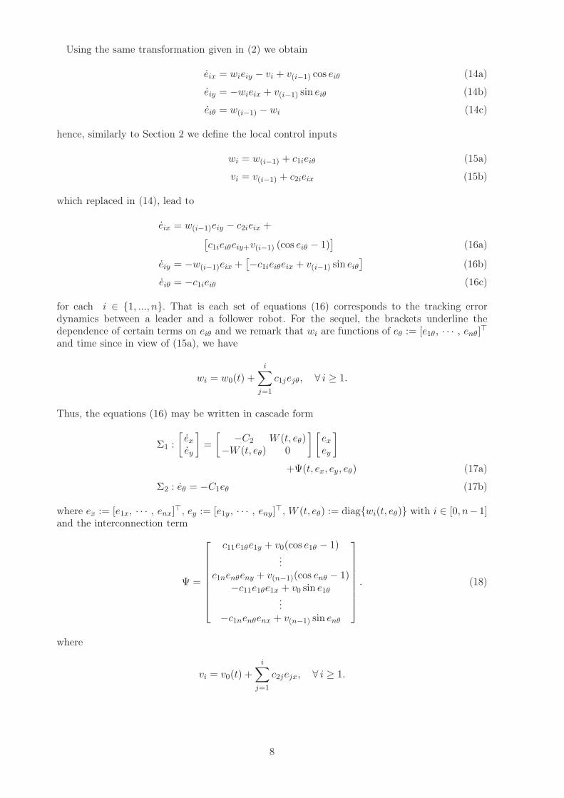
Using the same transformation given in (2) we obtain

eix = wieiy − vi + v(i−1) cos eiθ (14a)

eiy = −wieix + v(i−1) sin eiθ (14b)

eiθ = w(i−1) − wi (14c)

hence, similarly to Section 2 we define the local control inputs

wi = w(i−1) + c1ieiθ (15a)

vi = v(i−1) + c2ieix (15b)

which replaced in (14), lead to

eix = w(i−1)eiy − c2ieix +[

c1ieiθeiy+v(i−1) (cos eiθ − 1)]

(16a)

eiy = −w(i−1)eix +[

−c1ieiθeix + v(i−1) sin eiθ]

(16b)

eiθ = −c1ieiθ (16c)

for each i ∈ {1, ..., n}. That is each set of equations (16) corresponds to the tracking errordynamics between a leader and a follower robot. For the sequel, the brackets underline thedependence of certain terms on eiθ and we remark that wi are functions of eθ := [e1θ, · · · , enθ]⊤and time since in view of (15a), we have

wi = w0(t) +

i∑

j=1

c1jejθ, ∀ i ≥ 1.

Thus, the equations (16) may be written in cascade form

Σ1 :

[

exey

]

=

[

−C2 W (t, eθ)−W (t, eθ) 0

] [

exey

]

+Ψ(t, ex, ey, eθ) (17a)

Σ2 : eθ = −C1eθ (17b)

where ex := [e1x, · · · , enx]⊤, ey := [e1y , · · · , eny]⊤, W (t, eθ) := diag{wi(t, eθ)} with i ∈ [0, n−1]and the interconnection term

Ψ =

c11e1θe1y + v0(cos e1θ − 1)...

c1nenθeny + v(n−1)(cos enθ − 1)−c11e1θe1x + v0 sin e1θ

...−c1nenθenx + v(n−1) sin enθ

. (18)

where

vi = v0(t) +

i∑

j=1

c2jejx, ∀ i ≥ 1.

8

Note that Ψ(t, ex, ey, 0) ≡ 0.We are ready to present our first result.

Proposition 3.1: Consider the system (14) in closed loop with the controllers (15) with i ∈{1, ...n} where c1i, c2i > 0 and assume that

max{supt≥0

|v0(t)| , supt≥0

|w0(t)| , supt≥0

|w0(t)|} ≤ bµ (19)

for some bµ > 0. Then, the origin of the closed-loop system is uniformly globally exponentiallystable if and only if w0 is persistently exciting.

Proof The closed loop dynamics is given by (17) therefore, we must show that the origin of thesystem is uniformly globally exponentially stable and that persistency of excitation of w0 is anecessary condition. We proceed by invoking Theorem 6.1 from the Appendix.

Let x1 := [ex, ey ]⊤, x2 := eθ,

f1(t, x) :=

[

−C2 W (t, 0)−W (t, 0) 0

] [

exey

]

(20)

where W (t, 0) := w0(t)I, C1 := diag {c1i} , C2 := diag {c2i},

g(t, x) = Ψ(t, ex, ey, eθ) +[

0 W (t, eθ)−W (t, 0)−W (t, eθ) +W (t, 0) 0

] [

exey

]

and f2(t, x2) := −C1eθ. That is, the closed-loop dynamics (17) has the form (4). It is clear thatthe regularity assumptions on f1 and f2 (see the Appendix) hold in view of (19). Now, uniformglobal exponential stability of the origin of x1 = f1(t, x1) follows from Theorem 2.1 under theconditions of the proposition. On the other hand, uniform global exponential stability of theorigin of (17b) is evident since C1 is diagonal positive definite.

It remains to show that Assumptions A1 and A2 of Theorem 6.1 in the Appendix hold. As-sumption A1 holds with

V (t, x1) =1

2

[

|ex|2 + |ey|2]

, (21)

c1 = 2 and c2 = 1 = η = 1. The total time-derivative of V along the trajectories of x1 = f1(t, x1)where f1 is defined in (20), yields

V (t, x1) = −e⊤xC2ex ≤ 0.

Finally, Assumption A2 holds in view of the fact that x2 = 0 implies that g = 0 for any t ≥ 0and x1 ∈ R

2n and both Ψ and W (t, eθ)−W (t, 0) are both linear in [ex ey] and uniformly boundedin t, the latter comes from (19). �

9

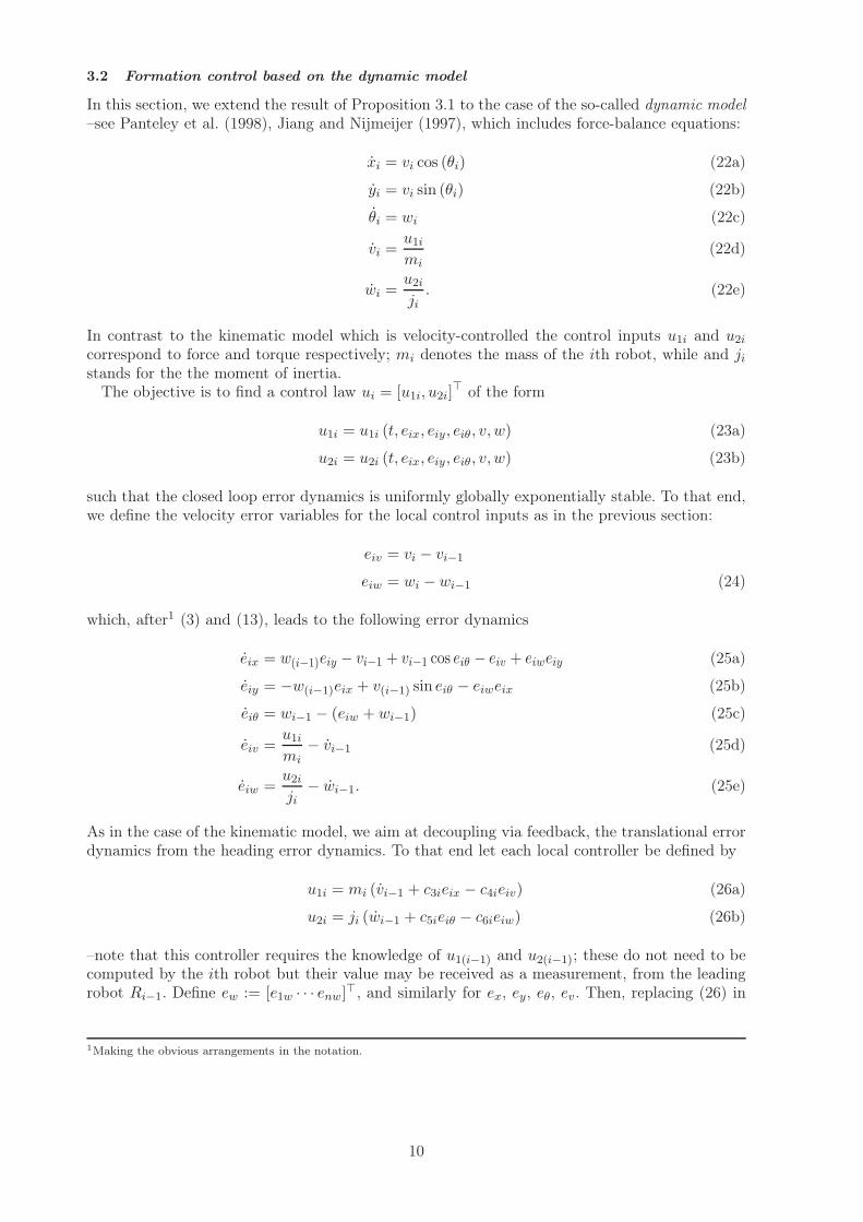
3.2 Formation control based on the dynamic model

In this section, we extend the result of Proposition 3.1 to the case of the so-called dynamic model–see Panteley et al. (1998), Jiang and Nijmeijer (1997), which includes force-balance equations:

xi = vi cos (θi) (22a)

yi = vi sin (θi) (22b)

θi = wi (22c)

vi =u1imi

(22d)

wi =u2iji

. (22e)

In contrast to the kinematic model which is velocity-controlled the control inputs u1i and u2icorrespond to force and torque respectively; mi denotes the mass of the ith robot, while and jistands for the the moment of inertia.

The objective is to find a control law ui = [u1i, u2i]⊤ of the form

u1i = u1i (t, eix, eiy, eiθ, v, w) (23a)

u2i = u2i (t, eix, eiy, eiθ, v, w) (23b)

such that the closed loop error dynamics is uniformly globally exponentially stable. To that end,we define the velocity error variables for the local control inputs as in the previous section:

eiv = vi − vi−1

eiw = wi − wi−1 (24)

which, after1 (3) and (13), leads to the following error dynamics

eix = w(i−1)eiy − vi−1 + vi−1 cos eiθ − eiv + eiweiy (25a)

eiy = −w(i−1)eix + v(i−1) sin eiθ − eiweix (25b)

eiθ = wi−1 − (eiw + wi−1) (25c)

eiv =u1imi

− vi−1 (25d)

eiw =u2iji

− wi−1. (25e)

As in the case of the kinematic model, we aim at decoupling via feedback, the translational errordynamics from the heading error dynamics. To that end let each local controller be defined by

u1i = mi (vi−1 + c3ieix − c4ieiv) (26a)

u2i = ji (wi−1 + c5ieiθ − c6ieiw) (26b)

–note that this controller requires the knowledge of u1(i−1) and u2(i−1); these do not need to becomputed by the ith robot but their value may be received as a measurement, from the leadingrobot Ri−1. Define ew := [e1w · · · enw]⊤, and similarly for ex, ey, eθ, ev. Then, replacing (26) in

1Making the obvious arrangements in the notation.

10

(25) and using wi−1 = wi − eiw we obtain by direct computation,

eix = wi(t, ew)eiy − eiv + vi−1[cos eiθ − 1] (27a)

eiy = −wi(t, ew)eix + v(i−1) sin eiθ (27b)

eiθ = −eiw (27c)

eiv = c3ieix − c4ieiv (27d)

eiw = c5ieiθ − c6ieiw. (27e)

We stress that for any i, wi is a function of ew and time, indeed in view of (24) we have w1 =e1w +w0(t), w2 = e2w + e1w + w0(t) and

wi = eiw + e(i−1)w + · · ·+ e1w + w0(t), ∀ i ≥ 3.

The system (27) has a cascades structure reminiscent of (17) in which the translation errordynamics is decoupled from the heading error dynamics. To see this, we first remark that thetranslation error dynamics may be rewritten in the compact form

exevey

=

0 −I W (t, ew)C3 −C4 0

−W (t, ew) 0 0

exevey

+Ψ2 (t, ev, eθ) (28)

where W (t, ew) = diag{wi(t, ew)}, C3 := diag{c3i}, C4 := diag{c4i} and the interconnection termis given by

Ψ2=

(Coseθ − I)vSineθv0n×1

(29)

where v := [v0 · · · vn−1]⊤, Coseθ := diag{cos eiθ} and Sineθ := diag{sin eiθ} and note that each

vi = eiv + e(i−1)v + · · ·+ e1v + v0(t), ∀ i ≥ 3

hence v is a function of t and ev. We also remark that Ψ2(t, ev , 0) ≡ 0. Finally, the heading errordynamics given by equations (27c) and (27e), become

[

eθew

]

=

[

0 −IC5 −C6

] [

eθew

]

(30)

where C5 := diag{c5i} and C6 := diag{c6i}. We recognize the desired cascaded structure; we areready to present our second result.

Proposition 3.2: Consider the system (22) in closed loop with the controllers (26) with i ∈{1, ...n} where c3i, c4i, c5i, c6i > 0 and the references v0 and w0 satisfy (19). Then, the origin ofthe closed-loop system is uniformly globally exponentially stable if and only if (11) holds.

Proof The closed loop dynamics is given by (28), (30) therefore, we must show that the originof this system is uniformly globally exponentially stable and that persistency of excitation of w0

is a necessary condition. As for Proposition 3.1 we rely on Theorem 6.1 from the Appendix. Let

11

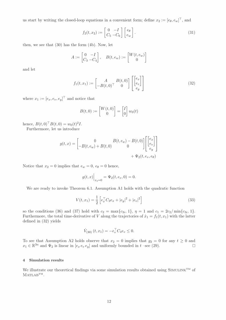
us start by writing the closed-loop equations in a convenient form; define x2 := [eθ, ew]⊤, and

f2(t, x2) :=

[

0 −IC5 −C6

] [

eθew

]

. (31)

then, we see that (30) has the form (4b). Now, let

A :=

[

0 −IC3 −C4

]

, B(t, ew) :=

[

W (t, ew)0

]

and let

f1(t, x1) :=

[

A B(t, 0)−B(t, 0)⊤ 0

]

[

exev

]

ey

(32)

where x1 := [ex, ev, ey]⊤ and notice that

B(t, 0) :=

[

W (t, 0)0

]

=

[

I0

]

w0(t)

hence, B(t, 0)⊤B(t, 0) = w0(t)2I.

Furthermore, let us introduce

g(t, x) =

[

0 B(t, ew)−B(t, 0)−B(t, ew) +B(t, 0) 0

]

[

exev

]

ey

+Ψ2(t, ev , eθ)

Notice that x2 = 0 implies that ew = 0, eθ = 0 hence,

g(t, x)∣

∣

∣

x2=0= Ψ2(t, ev , 0) = 0.

We are ready to invoke Theorem 6.1. Assumption A1 holds with the quadratic function

V (t, x1) =1

2

[

e⊤xC3ex + |ey|2 + |ev|2]

(33)

so the conditions (36) and (37) hold with c2 = max{c3i, 1}, η = 1 and c1 = 2c2/min{c3i, 1}.Furthermore, the total time-derivative of V along the trajectories of x1 = f1(t, x1) with the latterdefined in (32) yields

V(30) (t, x1) = −e⊤v C4ev ≤ 0.

To see that Assumption A2 holds observe that x2 = 0 implies that g2 = 0 for any t ≥ 0 andx1 ∈ R

3n and Ψ2 is linear in [ex ev ey] and uniformly bounded in t –see (29). �

4 Simulation results

We illustrate our theoretical findings via some simulation results obtained using SimulinkTM ofMatlab

TM.

12

−8 −6 −4 −2 0 2 4 6−2

0

2

4

6

8

10

12

t=0

t=10

t=70

x (m)

y (m

)

R3

R4

R1

R5

R2

(a) Triangular formation

−5 0 5

−2

0

2

4

6

8

10

12

t=70

t=80

t=90

t=100

x (m)

y (m

)

(b) Alined formation

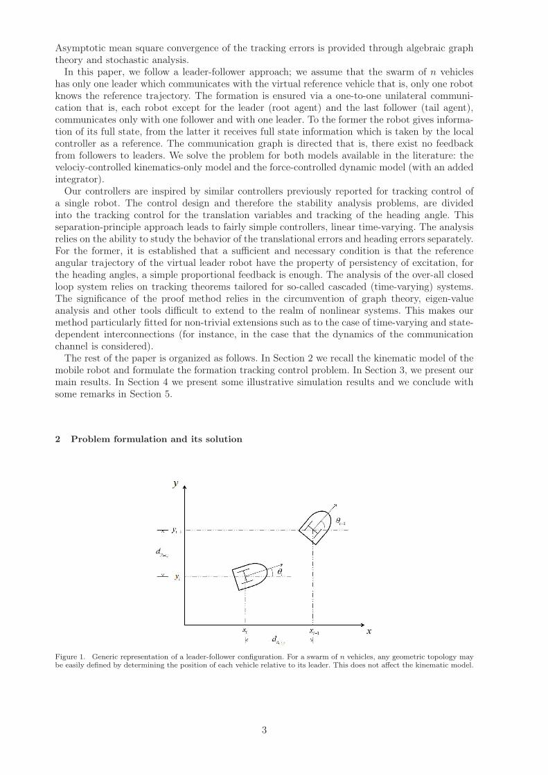
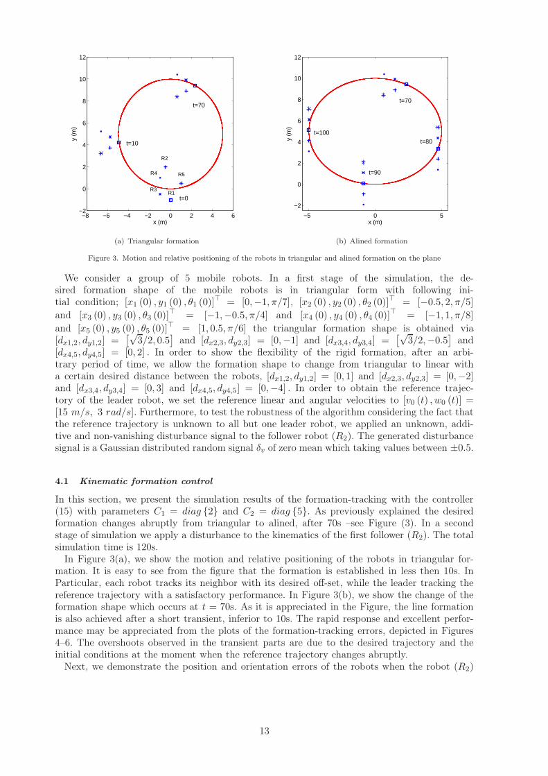
Figure 3. Motion and relative positioning of the robots in triangular and alined formation on the plane

We consider a group of 5 mobile robots. In a first stage of the simulation, the de-sired formation shape of the mobile robots is in triangular form with following ini-tial condition; [x1 (0) , y1 (0) , θ1 (0)]

⊤ = [0,−1, π/7], [x2 (0) , y2 (0) , θ2 (0)]⊤ = [−0.5, 2, π/5]

and [x3 (0) , y3 (0) , θ3 (0)]⊤ = [−1,−0.5, π/4] and [x4 (0) , y4 (0) , θ4 (0)]

⊤ = [−1, 1, π/8]

and [x5 (0) , y5 (0) , θ5 (0)]⊤ = [1, 0.5, π/6] the triangular formation shape is obtained via

[dx1,2, dy1,2] =[√

3/2, 0.5]

and [dx2,3, dy2,3] = [0,−1] and [dx3,4, dy3,4] =[√

3/2,−0.5]

and[dx4,5, dy4,5] = [0, 2] . In order to show the flexibility of the rigid formation, after an arbi-trary period of time, we allow the formation shape to change from triangular to linear witha certain desired distance between the robots, [dx1,2, dy1,2] = [0, 1] and [dx2,3, dy2,3] = [0,−2]and [dx3,4, dy3,4] = [0, 3] and [dx4,5, dy4,5] = [0,−4] . In order to obtain the reference trajec-tory of the leader robot, we set the reference linear and angular velocities to [v0 (t) , w0 (t)] =[15 m/s, 3 rad/s]. Furthermore, to test the robustness of the algorithm considering the fact thatthe reference trajectory is unknown to all but one leader robot, we applied an unknown, addi-tive and non-vanishing disturbance signal to the follower robot (R2). The generated disturbancesignal is a Gaussian distributed random signal δv of zero mean which taking values between ±0.5.

4.1 Kinematic formation control

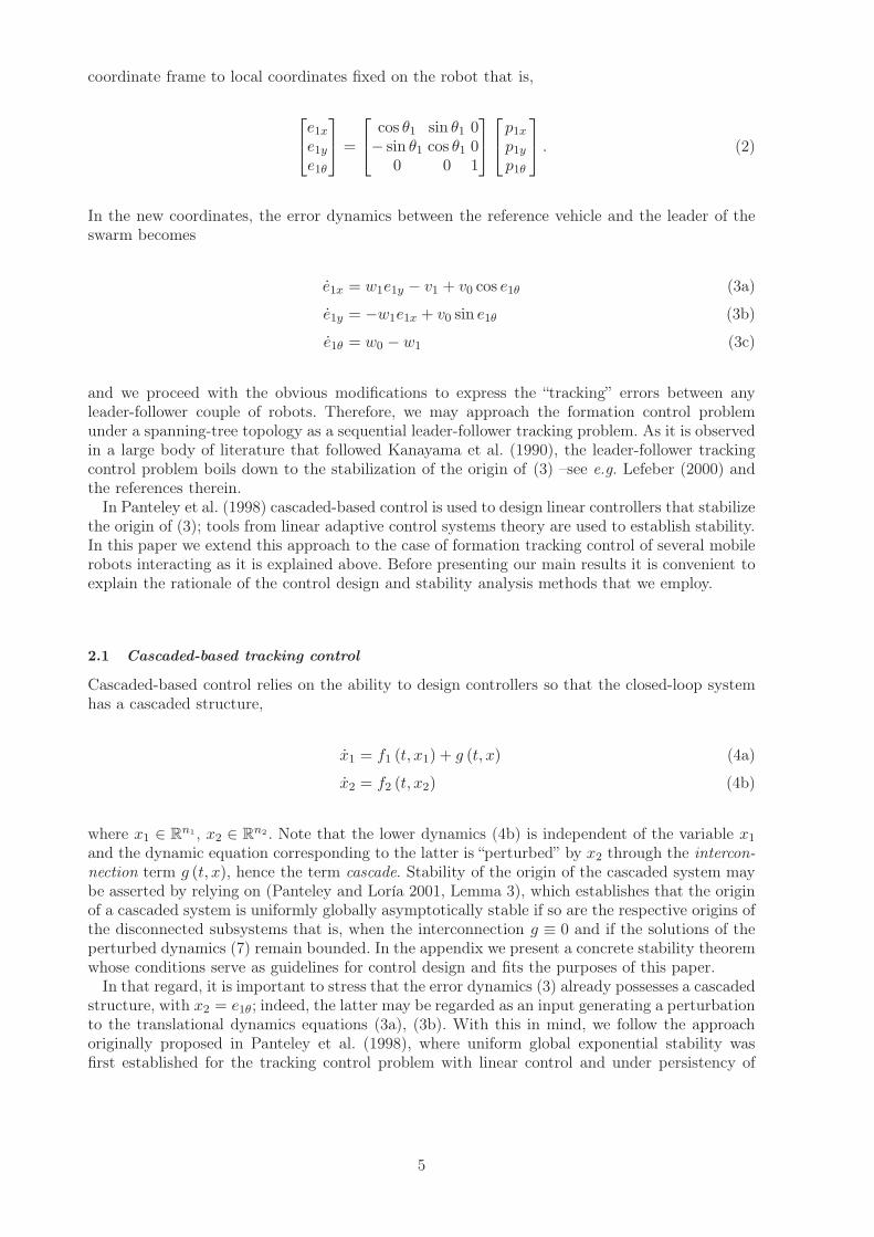
In this section, we present the simulation results of the formation-tracking with the controller(15) with parameters C1 = diag {2} and C2 = diag {5}. As previously explained the desiredformation changes abruptly from triangular to alined, after 70s –see Figure (3). In a secondstage of simulation we apply a disturbance to the kinematics of the first follower (R2). The totalsimulation time is 120s.

In Figure 3(a), we show the motion and relative positioning of the robots in triangular for-mation. It is easy to see from the figure that the formation is established in less then 10s. InParticular, each robot tracks its neighbor with its desired off-set, while the leader tracking thereference trajectory with a satisfactory performance. In Figure 3(b), we show the change of theformation shape which occurs at t = 70s. As it is appreciated in the Figure, the line formationis also achieved after a short transient, inferior to 10s. The rapid response and excellent perfor-mance may be appreciated from the plots of the formation-tracking errors, depicted in Figures4–6. The overshoots observed in the transient parts are due to the desired trajectory and theinitial conditions at the moment when the reference trajectory changes abruptly.

Next, we demonstrate the position and orientation errors of the robots when the robot (R2)

13

0 20 40 60 80 100 120−3

−2

−1

0

1

2

3

t (sec)

e 1x(t

), e

2x(t

), e

3x(t

),e 4x

(t),

e5x

(t)

Position errors in x coordinate

e1x

(t)

e2x

(t)

e3x

(t)

e4x

(t)

e5x

(t)

Figure 4. Position errors in x coordinates with kinematic control algorithm.

0 20 40 60 80 100 120−6

−4

−2

0

2

4

t (sec)

e 1y(t

), e

2y(t

), e

3y(t

),e 4y

(t),

e5y

(t)

Position errors in y coordinate

e

1y(t)

e2y

(t)

e3y

(t)

e4y

(t)

e5y

(t)

Figure 5. Position errors in y coordinates with kinematic control algorithm.

0 20 40 60 80 100 120−0.5

−0.4

−0.3

−0.2

−0.1

0

0.1

0.2

0.3

0.4

t (sec)

e 1θ(t

), e

2θ(t

), e

3θ(t

),

e 4θ(t

), e

5θ(t

)

Heading errors

e1θ

(t)

e2θ

(t)

e3θ

(t)

e4θ

(t)

e5θ

(t)

Figure 6. Heading errors with kinematic control algorithm.

is subjected to an additive, non-vanishing disturbance with their zoom in on the transient partof their responses. As it may be appreciated from Figures 7–8 the controlled system is robust inthe sense that the steady-state error is kept considerably small. The effect of the disturbances onthe orientation error is null and therefore it is not showed. As expected from the communicationtopology (spanning tree) and from our main result, the response of the global leader does notchange. Because the position errors of the follower robot (R2) converge to a small neighborhoodof the origin, the performance of the latter robots are very satisfactory.

14

0 20 40 60 80 100 120−3

−2

−1

0

1

2

3

t (sec)

e 1x(t

), e

2x(t

), e

3x(t

),

e 4x(t

), e

5x(t

)

Position errors in x coordinate

100 110 120

−0.01

0

0.01

20 25 30 35 40

−0.01

0

0.01

e1x

(t)

e2x

(t)

e3x

(t)

e4x

(t)

e5x

(t)

Figure 7. Position errors in x coordinates with kinematic control algorithm under disturbance.

0 20 40 60 80 100 120−6

−4

−2

0

2

4

t (sec)

e 1y(t

), e

2y(t

), e

3y(t

),

e 4y(t

), e

5y(t

)

Position errors in y coordinate

100 110 120

−0.01

0

0.01

20 30 40

−0.01

0

0.01

e1y

(t)

e2y

(t)

e3y

(t)

e4y

(t)

e5y

(t)

Figure 8. Position errors in y coordinates with kinematic control algorithm under disturbance.

4.2 Dynamic formation control

Now we present numerical simulation results on formation-tracking for systems modelled by(22), under the controller (26). The controller gains are fixed to C3 = diag {12, 17, 17, 17, 17},C4 = diag {5} and C5 = C6 = diag {10}. For the sake of consistency, we repeat the previousscenario: the desired triangular formation changes to aline-formation after 70s then, we apply adisturbance δv to the robot (R2).

0 20 40 60 80 100 120−5

−4

−3

−2

−1

0

1

2

3

4

t (sec)

e 1x(t

), e

2x(t

), e

3x(t

),

e 4x(t

), e

5x(t

)

Position errors in x coordinate

e

1x(t)

e2x

(t)

e3x

(t)

e4x

(t)

e5x

(t)

Figure 9. Position errors in x coordinates with dynamic control algorithm.

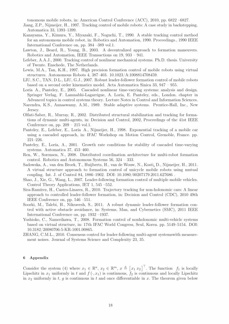
The simulation results are depicted in Figures 9–13. In Figures 9–11 one may appreciate thefast response and the exponential convergence of the errors in the absence of disturbances. Inthe last two figures we illustrate the robustness of the controlled system, subject to the effect

15

0 20 40 60 80 100 120−6

−4

−2

0

2

4

t (sec)

e 1y(t

), e

2y(t

), e

3y(t

),

e 4y(t

), e

5y(t

)

Position errors in y coordinate

e1y

(t)

e2y

(t)

e3y

(t)

e4y

(t)

e5y

(t)

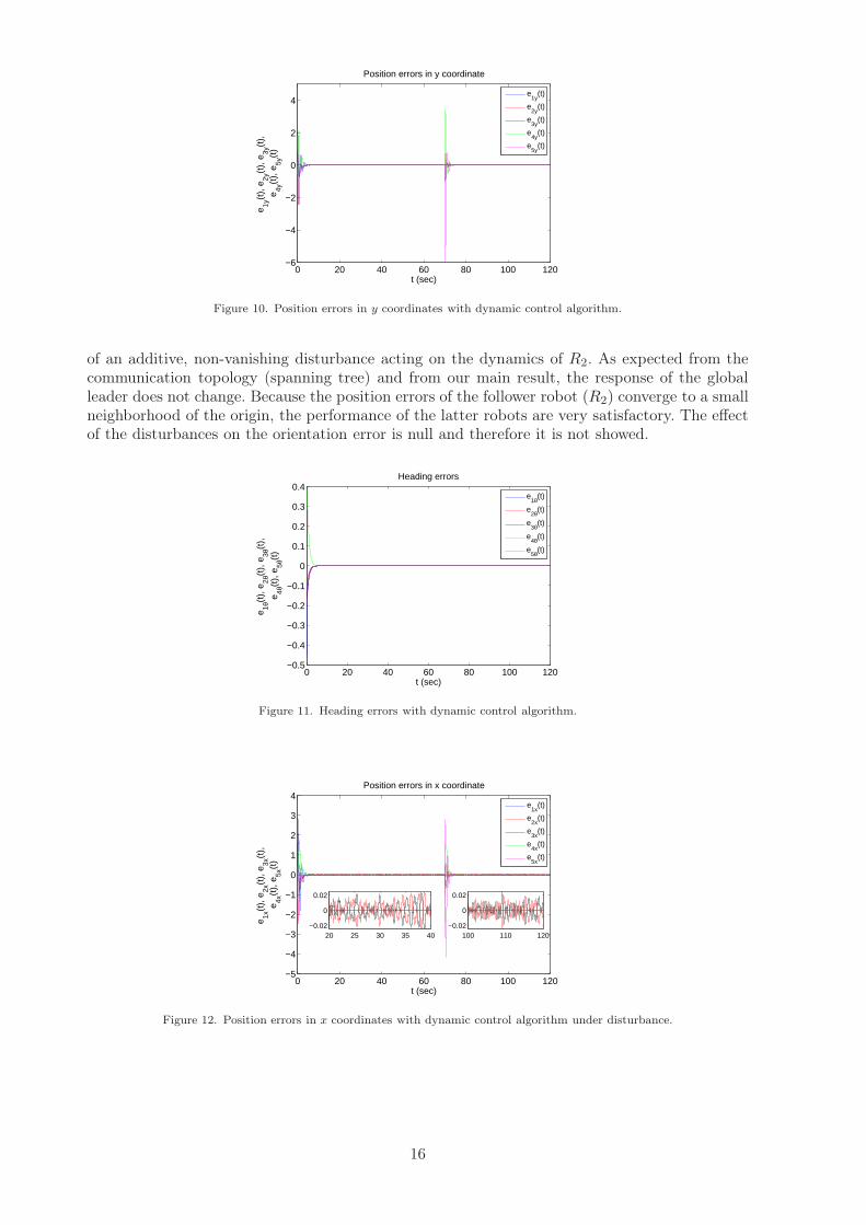
Figure 10. Position errors in y coordinates with dynamic control algorithm.

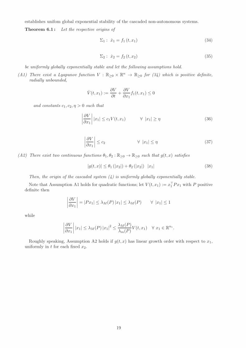
of an additive, non-vanishing disturbance acting on the dynamics of R2. As expected from thecommunication topology (spanning tree) and from our main result, the response of the globalleader does not change. Because the position errors of the follower robot (R2) converge to a smallneighborhood of the origin, the performance of the latter robots are very satisfactory. The effectof the disturbances on the orientation error is null and therefore it is not showed.

0 20 40 60 80 100 120−0.5

−0.4

−0.3

−0.2

−0.1

0

0.1

0.2

0.3

0.4

t (sec)

e 1θ(t

), e

2θ(t

), e

3θ(t

),

e 4θ(t

), e

5θ(t

)

Heading errors

e1θ

(t)

e2θ

(t)

e3θ

(t)

e4θ

(t)

e5θ

(t)

Figure 11. Heading errors with dynamic control algorithm.

0 20 40 60 80 100 120−5

−4

−3

−2

−1

0

1

2

3

4

t (sec)

e 1x(t

), e

2x(t

), e

3x(t

),

e 4x(t

), e

5x(t

)

Position errors in x coordinate

100 110 120−0.02

0

0.02

20 25 30 35 40−0.02

0

0.02

e1x

(t)

e2x

(t)

e3x

(t)

e4x

(t)

e5x

(t)

Figure 12. Position errors in x coordinates with dynamic control algorithm under disturbance.

16

0 20 40 60 80 100 120−6

−4

−2

0

2

4

t (sec)

e 1y(t

), e

2y(t

), e

3y(t

),

e 4y(t

), e

5y(t

)

Position errors in y coordinate

100 110 120−0.02

0

0.02

20 25 30 35 40−0.02

0

0.02

e1y

(t)

e2y

(t)

e3y

(t)

e4y

(t)

e5y

(t)

Figure 13. Position errors in y coordinates with dynamic control algorithm under disturbance.

5 Conclusion

We have presented a simple linear controller for formation tracking of a swarm of nonholonomicrobots interconnected in a spanning-tree communication configuration. The formation topologyis arbitrary and the main assumption is that the angular velocity is persistently exciting. Currentwork is carried out to extend ourresults to the case of time-varying topology that is, consideringthat the interconnections are not constant but time-varying or even state-dependent.

Acknowledgements

The work of the first author was supported by the Scientific and Technological Research Councilof Turkey (TUBITAK) BIDEB under the programme 2219 and was realized while she was onleave at L2S, Supelec, France.

References

Balch, T., Arkin, R., 1998. Behavior-based formation control for multirobot teams. Roboticsand Automation, IEEE Transactions on 14, 926 –939.

Consolini, L., Morbidi, F., Prattichizzo, D., Tosques, M., 2008. Leader–follower formation controlof nonholonomic mobile robots with input constraints. Automatica 44, 1343 – 1349.

Desai, J., Ostrowski, J., Kumar, V., 2001. Modeling and control of formations of nonholonomicmobile robots. Robotics and Automation, IEEE Transactions on 17, 905 –908.

Dierks, T., Brenner, B., Jagannathan, S., 2012. Neural network-based optimal control of mobilerobot formations with reduced information exchange. Control Systems Technology, IEEETransactions on PP, 1.

Dong, W., Guo, Y., Farrell, J., 2006. Formation control of nonholonomic mobile robots, in:American Control Conference, 2006, p. 6 pp.

Fax, J., Murray, R., 2004. Information flow and cooperative control of vehicle formations. Auto-matic Control, IEEE Transactions on 49, 1465 – 1476.

Fierro, R., Das, A., Kumar, V., Ostrowski, J., 2001. Hybrid control of formations of robots, in:Robotics and Automation, 2001. Proceedings 2001 ICRA. IEEE International Conference on,pp. 157 – 162 vol.1.

Gamage, G., Mann, G., Gosine, R., 2010. Leader follower based formation control strategies fornonholonomic mobile robots: Design, implementation and experimental validation, in: Ameri-can Control Conference (ACC), 2010, pp. 224 –229.

Ghommam, J., Mehrjerdi, H., Saad, M., 2011. Leader-follower based formation control of non-holonomic robots using the virtual vehicle approach, in: Mechatronics (ICM), 2011 IEEE In-ternational Conference on, pp. 516 –521.

Guo, J., Lin, Z., Cao, M., Yan, G., 2010. Adaptive leader-follower formation control for au-

17

tonomous mobile robots, in: American Control Conference (ACC), 2010, pp. 6822 –6827.Jiang, Z.P., Nijmeijer, H., 1997. Tracking control of mobile robots: A case study in backstepping.

Automatica 33, 1393–1399.Kanayama, Y., Kimura, Y., Miyazaki, F., Noguchi, T., 1990. A stable tracking control method

for an autonomous mobile robot, in: Robotics and Automation, 1990. Proceedings., 1990 IEEEInternational Conference on, pp. 384 –389 vol.1.

Lawton, J., Beard, R., Young, B., 2003. A decentralized approach to formation maneuvers.Robotics and Automation, IEEE Transactions on 19, 933 – 941.

Lefeber, A.A.J., 2000. Tracking control of nonlinear mechanical systems. Ph.D. thesis. Universityof Twente. Enschede, The Netherlands.

Lewis, M.A., Tan, K.H., 1997. High precision formation control of mobile robots using virtualstructures. Autonomous Robots 4, 387–403. 10.1023/A:1008814708459.

LIU, S.C., TAN, D.L., LIU, G.J., 2007. Robust leader-follower formation control of mobile robotsbased on a second order kinematics model. Acta Automatica Sinica 33, 947 – 955.

Loría A., Panteley, E., 2005. Cascaded nonlinear time-varying systems: analysis and design.Springer Verlag, F. Lamnabhi-Lagarrigue, A. Loría, E. Panteley, eds., London. chapter inAdvanced topics in control systems theory. Lecture Notes in Control and Information Sciences.

Narendra, K.S., Annaswamy, A.M., 1989. Stable adaptive systems. Prentice-Hall, Inc., NewJersey.

Olfati-Saber, R., Murray, R., 2002. Distributed structural stabilization and tracking for forma-tions of dynamic multi-agents, in: Decision and Control, 2002, Proceedings of the 41st IEEEConference on, pp. 209 – 215 vol.1.

Panteley, E., Lefeber, E., Loría A., Nijmeijer, H., 1998. Exponential tracking of a mobile carusing a cascaded approach, in: IFAC Workshop on Motion Control, Grenoble, France. pp.221–226.

Panteley, E., Loría, A., 2001. Growth rate conditions for stability of cascaded time-varyingsystems. Automatica 37, 453–460.

Ren, W., Sorensen, N., 2008. Distributed coordination architecture for multi-robot formationcontrol. Robotics and Autonomous Systems 56, 324 – 333.

Sadowska, A., van den Broek, T., Huijberts, H., van de Wouw, N., Kosti, D., Nijmeijer, H., 2011.A virtual structure approach to formation control of unicycle mobile robots using mutualcoupling. Int. J. of Control 84, 1886–1902. DOI: 10.1080/00207179.2011.627686 .

Shao, J., Xie, G., Wang, L., 2007. Leader-following formation control of multiple mobile vehicles.Control Theory Applications, IET 1, 545 –552.

Sira-Ramírez, H., Castro-Linares, R., 2010. Trajectory tracking for non-holonomic cars: A linearapproach to controlled leader-follower formation, in: Decision and Control (CDC), 2010 49thIEEE Conference on, pp. 546 –551.

Soorki, M., Talebi, H., Nikravesh, S., 2011. A robust dynamic leader-follower formation con-trol with active obstacle avoidance, in: Systems, Man, and Cybernetics (SMC), 2011 IEEEInternational Conference on, pp. 1932 –1937.

Yoshioko, C., Namerikawa, T., 2008. Formation control of nonholonomic multi-vehicle systemsbased on virtual structure, in: 17th IFAC World Congress, Seul, Korea. pp. 5149–5154. DOI:10.3182/20080706-5-KR-1001.00865.

ZHANG, C.M.L., 2010. Consensus control for leader-following multi-agent systemswith measure-ment noises. Journal of Systems Science and Complexity 23, 35.

6 Appendix

Consider the system (4) where x1 ∈ Rn, x2 ∈ R

m, x ,[

x1 x2]⊤

. The function f1 is locallyLipschitz in x1 uniformly in t and f (·, x1) is continuous, f2 is continuous and locally Lipschitzin x2 uniformly in t, g is continuous in t and once differentiable in x. The theorem given below

18

establishes unifom global exponential stability of the cascaded non-autonomous systems.

Theorem 6.1 : Let the respective origins of

Σ1 : x1 = f1 (t, x1) (34)

Σ2 : x2 = f2 (t, x2) (35)

be uniformly globally exponentially stable and let the following assumptions hold.

(A1) There exist a Lyapunov function V : R≥0 × Rn → R≥0 for (34) which is positive definite,

radially unbounded,

V (t, x1) :=∂V

∂t+

∂V

∂x1f1(t, x1) ≤ 0

and constants c1, c2, η > 0 such that

∣

∣

∣

∣

∂V

∂x1

∣

∣

∣

∣

|x1| ≤ c1V (t, x1) ∀ |x1| ≥ η (36)

∣

∣

∣

∣

∂V

∂x1

∣

∣

∣

∣

≤ c2 ∀ |x1| ≤ η (37)

(A2) There exist two continuous functions θ1, θ2 : R≥0 → R≥0 such that g(t, x) satisfies

|g(t, x)| ≤ θ1 (|x2|) + θ2 (|x2|) |x1| (38)

Then, the origin of the cascaded system (4) is uniformly globally exponentially stable.

Note that Assumption A1 holds for quadratic functions; let V (t, x1) := x⊤1 Px1 with P positivedefinite then

∣

∣

∣

∣

∂V

∂x1

∣

∣

∣

∣

= |Px1| ≤ λM (P ) |x1| ≤ λM (P ) ∀ |x1| ≤ 1

while

∣

∣

∣

∣

∂V

∂x1

∣

∣

∣

∣

|x1| ≤ λM (P ) |x1|2 ≤λM (P )

λm(P )V (t, x1) ∀ x1 ∈ R

n1 .

Roughly speaking, Assumption A2 holds if g(t, x) has linear growth order with respect to x1,uniformly in t for each fixed x2.

19