Abstract— A major issue in the field of mobile robotics today is the detection and tracking of moving objects (DATMO) from a moving observer. In dynamic and highly populated environments, this problem presents a complex and computationally demanding task. It can be divided in sub-problems such as robot’s relative motion compensation, feature extraction, measurement clustering, data association and targets’ state vector estimation. In this paper we present an innovative approach that addresses all these issues exploiting various probabilistic and deterministic techniques. The algorithm utilizes real laser-scanner data to dynamically extract moving objects from their background environment, using a time-fading grid map method, and tracks the identified targets employing a Joint Probabilistic Data Association with Interacting Multiple Model (JPDA-IMM) algorithm. The resulting technique presents a computationally efficient approach to already existing target-tracking research for real time application scenarios.

I. INTRODUCTION OR mobile robot applications that require to operate in dynamic and highly populated environments (e.g. museums, hospitals, etc.), it is imperative to identify and

track the trajectories of moving objects. Predicting environmental dynamics, using target tracking techniques, provides important information for navigational algorithms and improves robot responses to dynamic changes. Many previous approaches, which utilize 2D laser range scanner measurements, have dealt with the DATMO problem assuming that previous knowledge on the background and the targets is provided to the algorithm. In [1], a system for tracking pedestrians is described, using multiple stationary and sparsely-placed laser range scanners. A background is obtained beforehand and subtracted from each measurement frame in order to extract possible moving objects. A Kalman filter (KF) is implemented to track the extracted targets. In a different trail of thought, the authors in [2], [3] develop a feature detection system for real-time identification of geometric shapes such as lines, circles and legs from laser data and apply a KF for tracking. A similar but more sophisticated method can be found in [4]. Geometric profiles This work is supported by the FP6-Information Society Technologies program, European Commission INDIGO research project (Contract No. IST-045388).

are created on raw laser measurements, based on fourteen conditions. A classifier trained on these profiles, searches for specified patterns that can be categorized as legs. Grid-map approaches that employ laser data and particle filters for moving-object tracking can be found in [5], [6]. In both papers, a similar method is obtained that utilizes a series of occupancy grids for extracting moving objects in a dynamic environment. The authors introduce the sample-based Joint Probabilistic Data Association Filter (SJPDAF), which is an adapted version of JPDA algorithm suited for particle filter applications. Although both publications demonstrate effective usage of this technique, maintaining two consecutive probabilistic grid maps of robot’s space and additionally generating one map for every detected feature each time, is a process and memory expensive architecture. A grid map-free approach in presented in [7]. In this method, laser scanner measurements are either connected together in a closed polygon shape representing the free space, or as point samples of object surfaces. If such points are detected inside any previous polygon of free space, they are marked as moving object points. Odometry is employed to compensate the robot’s relative movement. Furthermore, statistical hypotheses are propagated using a gradient ascent method to track moving targets. The technique is tested with only one available moving target in space, thus its efficiency in multi-target tracking scenarios is unknown. Finally, a method for outdoor mobile robot applications is presented in [8]. It combines Simultaneous Localization and Mapping (SLAM) with DATMO to detect, categorize and track multiple moving targets in urban environments. This paper presents a new approach to DATMO problem framework. It blends the hybrid JPDA-IMM data association and tracking algorithm with an innovative occupancy-grid based approach for moving object detection. To extract and verify moving targets from stationary background, the proposed model follows a number of consecutive steps. Initially, a single occupancy-grid map is created. Every individual grid-cell accumulates a counter, which increases linearly when a laser measurement falls inside its occupancy area. Grid-cells with values above a dynamic threshold level are selected as stationary background. Moreover, all cells containing values above zero decrease linearly with time. A certain background is obtained and subtracted (utilizing

A Multi-Target Tracking Technique for Mobile Robots using a Laser Range Scanner

Polychronis Kondaxakis, Stathis Kasderidis, Panos Trahanias Institute of Computer Science

Foundation for Research and Technology – Hellas (FORTH) E-mail:{konda, stathis, trahania}@ics.forth.gr

F

2008 IEEE/RSJ International Conference on Intelligent Robots and SystemsAcropolis Convention CenterNice, France, Sept, 22-26, 2008

978-1-4244-2058-2/08/$25.00 ©2008 IEEE. 3370

covariance information) from every laser data frame leaving only the measurements that represent possible moving targets. The remaining measurements are clustered into groups and a centre of gravity is assigned to each one. Finally, the JPDA-IMM initiates and allocates tracks to clusters that exceed a certain velocity level. The resulting technique provides a processing and memory-efficient architecture and handles grid-map related problems such as map-size and transformation resolution.

II. STATIONARY BACKGROUND ATTENUATION

A. Laser Data Collection This research was conducted using a SICK LMS200 Laser

Range Scanner adjusted onboard a PIONEER 3-AT mobile robot platform. The scanner has an angular resolution of 0.5˚ and a span of 180˚ thus delivering 361 range readings per frame. Optimally, it can provide 25 frames per second at a maximum range of 60m with a resolution of ±5cm. Due to local wireless network limitations the scanner delivers about five measurement frames per second. Moreover, as a result of the indoor operational specifications in our experiments, the laser was adjusted to detect obstacles at a maximum of 9.6m distance. Measurements above 9.6m were ignored as outliers. We represent a measurement frame at time index k by a vector ( ) ( ) ( ) ( ){ }kkkklaser 36121 ,,, zzzZ K= , where ( )klz with

3611K=l , is a vector composed by distance and bearing readings, ( ) ( ) ( )[ ]Tlll kkrk ϕ,=z .

B. Mobile Robot’s Relative Movement Compensation Currently, there are large numbers of available publications in the field of real-time multi-object tracking techniques. However, the existing research publications decrease dramatically if the observer is also moving. In mobile robotic applications, relative movement compensation could be achieved by either synchronizing pure odometry readings with laser scanner measurements [7] or combining a SLAM algorithm with a DATMO system in a single framework, thus estimating at the same time both moving objects in the environment and robot’s trajectory [8]. This research utilizes an asynchronous distributed architecture where a number of subsystems (Localization module, Path-Planning module, DATMO module etc.) operate in parallel to obtain, upon request, the robot’s higher functionalities. It is well known that a vehicle with skid-steer drive configuration such as the PIONEER 3-AT is prompt to odometric errors. For that reason, the DATMO does not solidly utilize robot’s odometry. It rather exploits state and error covariance estimations, acquired from the localization algorithm [9], in order to compensate relative movement. The estimated state vector is composed by position (x, y) and orientation θ components, ( ) ( ) ( ) ( )[ ]TRRRR kkkkykkxkk θ̂,ˆ,ˆˆ =X .

Its associated estimated state error covariance matrix is given

by ( )kkRP . It has been assumed that an estimated state vector

is acquired simultaneously with every laser measurement frame, ( )klaserZ . Therefore, at discrete time index k, the robot’s state and laser measurement readings are bundled into a duple of vectors ( ) ( ) ( ){ }kkkkk RRlaser PXZ ,ˆ, . The algorithm

is configured to collect samples at approximately constant periodicity. The scan points are transformed in robot’s coordinate frame as follows:

( ) ( )( )

( ) ( ) ( )( ) ( )( ) ( ) ( )( ) ( )⎥⎥⎦

⎤

⎢⎢⎣

⎡

++++

=⎥⎦

⎤⎢⎣

⎡=

kkykkkkrkkxkkkkr

kykx

kRRll

RRll

l

ll ˆˆsin

ˆˆcos*

**

θϕθϕ

z (1)

with 3611K=l and ( ) ( ) ( ) ( ){ }kkkklaser*361

*2

*1

* ,,, zzzZ K= .

C. Occupancy Grid Map In DATMO research, a very popular method for isolating moving objects in dynamic environments, utilizes multiple occupancy grid maps [5], [6], [8]. Our novel approach employs a single accumulative occupancy grid for stationary feature extraction. This grid-map is dynamically updated for every laser measurement frame, ( )klaser

*Z . When new laser data become locally available to the robot, at a discrete time instant k with Ν∈k , they are translated in egocentric grid-map coordinates and assigned to cells. Every individual cell in the map maintains a counter, which increases linearly when a laser measurement vector, ( )kl

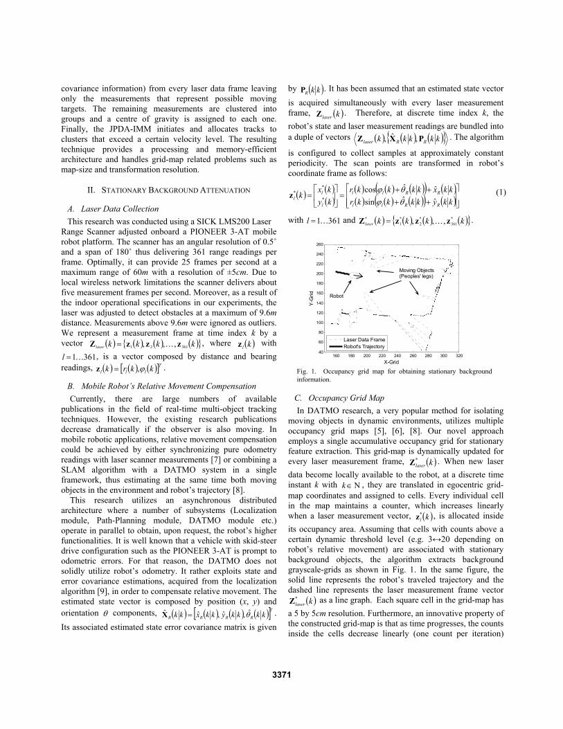
*z , is allocated inside its occupancy area. Assuming that cells with counts above a certain dynamic threshold level (e.g. 3↔20 depending on robot’s relative movement) are associated with stationary background objects, the algorithm extracts background grayscale-grids as shown in Fig. 1. In the same figure, the solid line represents the robot’s traveled trajectory and the dashed line represents the laser measurement frame vector

( )klaser*Z as a line graph. Each square cell in the grid-map has

a 5 by 5cm resolution. Furthermore, an innovative property of the constructed grid-map is that as time progresses, the counts inside the cells decrease linearly (one count per iteration)

X-Grid

Y-G

rid

160 180 200 220 240 260 280 300 32040

60

80

100

120

140

160

180

200

220

240

260

Laser Data FrameRobot's Trajectory

Moving Objects(Peoples' legs)

Robot

Fig. 1. Occupancy grid map for obtaining stationary background information.

3371

until they reach a zero value. In other words, if there is no positive laser measurement hits, grid counts tend to decrease at a constant rate. This technique dynamically updates the stationary background knowledge, limiting at the same time the required memory usage and processing power-consumption by the grid-map algorithm. Finally, the obtained background points are transformed back to robot’s local coordinate frame and supplied to the tracking algorithm for further processing. They are represented by vector

( ) ( ) ( ){ }kkk mbackground ρρV ,,1 K= ; where ( )koρ with mo K1= , is also a vector composed by x and y-stationary point components, ( ) ( ) ( )[ ]T

ooo kykxk ,=ρ . Fig 2. demonstrates the extracted background points in robot’s local coordinate axis.

D. Moving Target Detection To facilitate the detection of possible moving objects’ in

robot’s dynamic environment, the method deducts the background vector ( )kbackgroundV from a laser measurement frame ( )klaser

*Z , both obtained for time index k. Three major issues regarding the correct alignment of background and laser measurements are presented as follows: (i) The positional error and thus the relative error covariance estimates, increase as the mobile robot moves in space. (ii) The time required by this technique to readjust the dynamic background, increases as the robot moves. (iii) The laser measurement frame and dynamic background vectors are composed by different number of vector-points; hence one-to-one linear subtraction becomes prohibited. To resolve these issues, the proposed algorithm employs the following innovations.

Firstly, a dynamic threshold was introduced. It filters out possible moving targets from stationary objects by altering its condition according to robot’s state. If the robot is on the move, the threshold level decreases linearly with time until it reaches a minimum value (e.g. 3). Therefore, the dynamic background vector ( ( )kbackgroundV ), becomes more susceptible to rapid environmental changes. The opposite happens, when the mobile robot remains stationary. In that case, the

threshold level increases linearly with time until it reaches a maximum value (e.g. 20), thus rendering the background vector less sensitive to changes.

To counteract additional translation and rotation point-set differences between vectors ( )klaser

*Z and ( )kbackgroundV , an Iterative Closest Point (ICP) algorithm is employed. ICP is attractive because of its simplicity and its performance. Given two point sets A and B in R it minimizes a geometric distance function ( )BTAf ,+ , over all translations T. The algorithm starts with an arbitrary translation that aligns A to B, and then repeatedly performs local improvements that keep re-aligning A to B, while decreasing the distance function until a convergence is reached. Although the initial estimate does need to be reasonably good, the algorithm converges relatively quickly. A closed-form solution to the ICP algorithm can be found in [10]. However, our experimental results indicate that in many cases, discarding the ICP algorithm and running only with the dynamic threshold, provides the same or even better results. This is due to ICP’s inefficiency on large transformational changes. Finally, the tracking algorithm removes the measurement points from ( )klaser

*Z that are associated with vector points from ( )kbackgroundV utilizing the provided robot’s error covariance matrix estimation ( )kkRP and the laser-scanner’s

uncertainty model. Assuming the laser-scanner noise model in polar coordinates as [9]:

( )( )

( )⎥⎦⎤

⎢⎣

⎡+

=krkk

kkk

l

lpolarl

100

0

ρρ

ϕϕR (2)

where 10

,, ρρϕ kkk are parameters related to the range finder angular error, range error independent of distance, and distance-dependent range error, respectively. The transformation of Polar to Cartesian coordinates is:

( ) ( ) ( ) ( )kkkk Tpolarlcartl CRCR ∇∇= (3)

where ( )kC∇ is the Jacobean of ( )kl*z with respect to

( ) ( )[ ]kkr ll ϕ, . As it is evident from equations (2) and (3), the covariance of the sources of uncertainty and noise for the available measurement vector is a time-varying matrix. The values of the elements of this matrix depend on the measurement distance and bearing components. Averaging across all possible values of ( )klϕ and utilizing sensors’ maximum possible distance measurement ( mrl 6.9max = ), the noise covariance matrix ( )kcartlR becomes:

( ) ( )

( ) ( )⎥⎥⎥

⎦

⎤

⎢⎢⎢

⎣

⎡

++

++

=

20

02

max2max

max2max

10

10

lll

lll

cartl rkkkr

rkkkr

ρρϕ

ρρϕ

ϕ

ϕ

R

(4)

Equation (4) provides an averaged time-invariant expression

-8 -6 -4 -2 0 2-1

0

1

2

3

4

5

6

7

8Stationary Background

Dis

tanc

e in

m

Distance in m

Fig. 2. Extracted background in robot’s local coordinate frame.

3372

of (3) and will be used for a track initiation and maintenance process, in order to improve the algorithm’s calibration characteristics.

Finally, the overall error that describes the uncertainty of background point vectors is given by:

( ) ( ) ( )kkkk cartlTRRRbackl RHPHP += where

⎥⎦

⎤⎢⎣

⎡=

010001

RH (5)

A measurement point described by vector ( )kl*z is removed

if and only if the Mahalanobis distance to any of the vector points included in ( )kbackgroundV , is below a certain threshold λ resulting in:

( ) ( )[ ] ( )[ ] ( ) ( )[ ] λ≤−− − kkkkk mlbacklT

ml ,,2,1*1

,,2,1*

KK ρzPρz (6)

Therefore, the remaining moving object points are represented as ( ) ( ) ( ) ( ){ }kkkk smoving

**2

*1

* ,,, zzzZ K= with

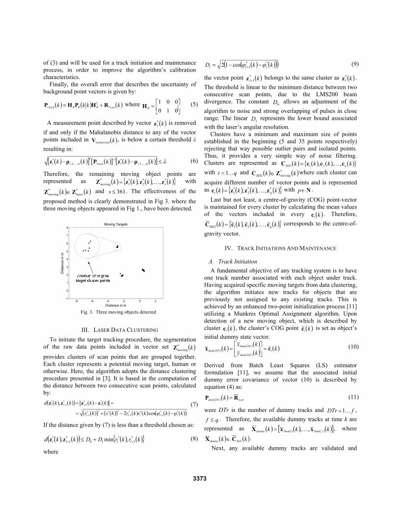
( ) ( )kk lasermoving** ZZ ∈ and 361≤s . The effectiveness of the

proposed method is clearly demonstrated in Fig 3. where the three moving objects appeared in Fig 1., have been detected.

III. LASER DATA CLUSTERING To initiate the target tracking procedure, the segmentation

of the raw data points included in vector set ( )kmoving*Z

provides clusters of scan points that are grouped together. Each cluster represents a potential moving target, human or otherwise. Here, the algorithm adopts the distance clustering procedure presented in [3]. It is based in the computation of the distance between two consecutive scan points, calculated by:

( ) ( )( ) ( ) ( )

( )( ) ( )( ) ( ) ( ) ( ) ( )( )kkkrkrkrkr

kkkkd

llllll

llll

**1

**1

2*2*1

**1

*1

*

cos2

,

ϕϕ −−+=

=−=

+++

++ zzzz (7)

If the distance given by (7) is less than a threshold chosen as:

( ) ( )( ) ( ) ( ){ }krkrDDkkd llll*

1*

10*

1* ,min, ++ +≤zz (8)

where

( ) ( )( )( )kkD ll**

11 cos12 ϕϕ −−= + (9)

the vector point ( )kl*

1+z belongs to the same cluster as ( )kl*z .

The threshold is linear to the minimum distance between two consecutive scan points, due to the LMS200 beam divergence. The constant 0D allows an adjustment of the algorithm to noise and strong overlapping of pulses in close range. The linear 1D represents the lower bound associated with the laser’s angular resolution. Clusters have a minimum and maximum size of points established in the beginning (5 and 35 points respectively) rejecting that way possible outlier pairs and isolated points. Thus, it provides a very simple way of noise filtering. Clusters are represented as ( ) ( ) ( ) ( ){ }kkkk qSEG cccC ,,, 21 K= with qt K1= and ( ) ( )kk movingSEG

*ZC ∈ where each cluster can

acquire different number of vector points and is represented as ( ) ( ) ( ) ( ){ }kkkk pt

**2

*1 ,,, zzzc K= with N∈p .

Last but not least, a centre-of-gravity (COG) point-vector is maintained for every cluster by calculating the mean values of the vectors included in every ( )ktc . Therefore,

( ) ( ) ( ) ( ){ }kkkk qSEG cccC ,,, 21 K= corresponds to the centre-of-

gravity vector.

IV. TRACK INITIATIONS AND MAINTENANCE

A. Track Initiation A fundamental objective of any tracking system is to have one track number associated with each object under track. Having acquired specific moving targets from data clustering, the algorithm initiates new tracks for objects that are previously not assigned to any existing tracks. This is achieved by an enhanced two-point initialization process [11] utilizing a Munkres Optimal Assignment algorithm. Upon detection of a new moving object, which is described by cluster ( )ktc , the cluster’s COG point ( )ktc is set as object’s initial dummy state vector.

( ) ( ) ( ) ( )( ) ( ) ( )k

kykx

k tDTrdum

DTrdumDTrdum cx =⎥

⎦

⎤⎢⎣

⎡= (10)

Derived from Batch Least Squares (LS) estimator formulation [11], we assume that the associated initial dummy error covariance of vector (10) is described by equation (4) as:

( ) ( ) lcartDTrdum k RP = (11)

were DTr is the number of dummy tracks and fDTr K1= , qf ≤ . Therefore, the available dummy tracks at time k are

represented as ( ) ( ) ( ) ( ) ( )[ ]kkk fDumDumdummy xxX ,,1 K= , where

( ) ( )kk SEGdummy CX ∈ . Next, any available dummy tracks are validated and

-8 -6 -4 -2 0 2-1

0

1

2

3

4

5

6

7

8

Dis

tanc

e in

m

Distance in m

Moving Targets

Fig. 3. Three moving objects detected

3373

promoted to verified-track status according to the following three-step procedure: 1. A measurement innovation matrix is calculated for every DTr based on the recursive LS estimator format [11]:

( ) lcartDTrdum k RS 21)( =+ (12)

It is worth mentioning here that the time-invariant equation (12) is obtained by substituting (4), which is assumed as the noise covariance of all targets at every time step, and (11) into LS estimator’s measurement innovation (Eq. 3.4.2-8 in [11]). For the same equation, measurement matrix H is a unit matrix.

2. A dummy track (DTr) is validated as a real track if and only if:

( ) ( ) ( )[ ] ( ) ( )[ ] ( ) ( ) ( )[ ] 11

0 111 γγ <−++−+< − kkkkk DTrdumtDTrdumT

DTrdumt xcSxc ,

qt K1= (13) where

10 ,γγ are the appropriate chi-squared threshold levels [12], which determine a statistical validation zone.

Employing two validation thresholds instead of one provides additional moving-object filtering to the system. To relate moving-objects’ speed to

10 ,γγ , the following expressions were used. First the validation region volume for minimum and maximum speeds, which is centered on the initial measurement cluster’s COG, is given by [13]:

( )[ ] ( )[ ]ylcart

xlcart RTyRTxVxy 3232 maxmin/maxmin/1/0 +×+= && (14)

where T is the sampling time interval and maxmin/x& , maxmin/y& are the minimum or maximum speeds in the X and Y directions respectively; x

lcartR , ylcartR are variances of position

measurements in these directions, obtained from the diagonal components of (4). In more general terms, the volume V of a validation region that corresponds to a threshold 1/0γ is:

( ) ( )kSckVxy zz

nn

21/01/0 γ= (15)

where zn is the dimension of the measurement and znc , is the

volume of the unit hypersphere of this dimension ( 21 =c , π=2c , 343 π=c , etc.). By substituting (12) and (14) into

(15) and solving with respect to 1/0γ we have:

( )[ ] ( )[ ]( )DTrdum

ylcart

xlcart RTyRTx

Sπγ 3232 maxmin/maxmin/

1/0

+×+=

&& (16)

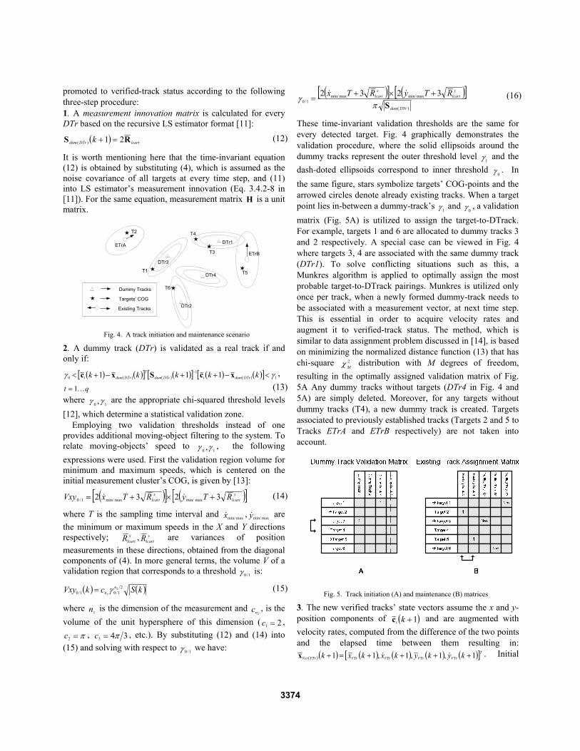
These time-invariant validation thresholds are the same for every detected target. Fig. 4 graphically demonstrates the validation procedure, where the solid ellipsoids around the dummy tracks represent the outer threshold level

1γ and the dash-doted ellipsoids correspond to inner threshold

0γ . In the same figure, stars symbolize targets’ COG-points and the arrowed circles denote already existing tracks. When a target point lies in-between a dummy-track’s

1γ and 0γ , a validation

matrix (Fig. 5A) is utilized to assign the target-to-DTrack. For example, targets 1 and 6 are allocated to dummy tracks 3 and 2 respectively. A special case can be viewed in Fig. 4 where targets 3, 4 are associated with the same dummy track (DTr1). To solve conflicting situations such as this, a Munkres algorithm is applied to optimally assign the most probable target-to-DTrack pairings. Munkres is utilized only once per track, when a newly formed dummy-track needs to be associated with a measurement vector, at next time step. This is essential in order to acquire velocity rates and augment it to verified-track status. The method, which is similar to data assignment problem discussed in [14], is based on minimizing the normalized distance function (13) that has chi-square 2

Mχ distribution with M degrees of freedom, resulting in the optimally assigned validation matrix of Fig. 5A Any dummy tracks without targets (DTr4 in Fig. 4 and 5A) are simply deleted. Moreover, for any targets without dummy tracks (T4), a new dummy track is created. Targets associated to previously established tracks (Targets 2 and 5 to Tracks ETrA and ETrB respectively) are not taken into account.

3. The new verified tracks’ state vectors assume the x and y-position components of ( )1+ktc and are augmented with velocity rates, computed from the difference of the two points and the elapsed time between them resulting in:

( ) ( ) ( ) ( ) ( ) ( )[ ]TVTrVTrVTrVTrVTrVer kykykxkxk 1,1,1,11 ++++=+ &&x . Initial

Fig. 5. Track initiation (A) and maintenance (B) matrices

T1

T2

T3

T6

DTr3

DTr4

DTr2

ETrA

T5

ETrB

T4

DTr1

Dummy Tracks

Targets’ COG

Existing Tracks

Fig. 4. A track initiation and maintenance scenario

3374

available tracks are represented by ( ) ( ) ( ) ( ) ( )[ ]1,,11 1 ++=+ kkk sVerVerverified xxX K with sVTr K1= . A

detailed explanation of the initial error covariance related to the new state vector is presented in [11].

B. Track Maintenance and Termination Before commencing new tracks for firstly-appeared

measurement clusters, a JPDA algorithm (see section V for detailed description) generates assignment hypothesis for pairing any unassociated COG’s in ( )kSEGC with the available existing tracks ( ) ( ) ( )[ ]kkkkkk aexisting xxX ˆ,,ˆˆ

1 K= . However,

maintaining track consistency requires a track-assignment matrix as the one displayed in Fig 5B. Continuing the scenario described in Fig. 4, the already established tracks ETrA and ETrB are assigned to targets 2 and 5. In the same matrix, any newly formulated tracks (eg. Track C, D, E) are started and placed at the end columns of the matrix for next-iteration use.

Verified tracks are divided into two categories: (a) Tracks with enhanced data-association performance, and (b) Tracks with reduced data-association performance. These two classes depend on how many association events have been accumulated by each track throughout its existing period. In other words, a linear counter assigned to every verified-track increases when the track is associated to a measurement cluster. Furthermore, as the track under examination remains unassociated, its counter decreases. Above a certain threshold, a track is considered as “enhanced” and it is regard as “more reliable” than tracks with less association hits than the threshold level.

Finally, tracks are considered obsolete and are terminated if they remain unassociated to measurement clusters for some specific period of time.

V. THE TRACKING ALGORITHM

A. Problem Formulation and Motion Models Suppose that the trajectories of the available targets are

described by ( )kkexistingX̂ estimated vector. Now assume that

the dynamics of each target can be modeled employing a number of n-hypothesized motion models denoted as

{ }nM n K,2,1:= . For the thj hypothesized model ( )(kjrM

active at time instant k), the state dynamics and measurements of target r are modeled using the standard state equations:

( ) ( ) ( ) ( ) ( )kkkkk jr

jrr

jrr wGxΦx +=+1 , nj K1= (17)

( ) ( ) ( ) ( )1111 ++++=+ kkkk jrr

jrr vxHz , ar K1= (18)

The state noise ( )kjrw and measurement noise ( )1+kj

rv are assumed to be independent with each other, independent of the state components, white (uncorrelated in time), and Gaussian distributed with zero-mean and covariance

( ) ( ) ( )[ ]Tjr

jr

jr kkEk wwQ = and ( ) ( ) ( )[ ]Tj

rjr

jr kkEk 111 ++=+ vvR

respectively. The system utilizes two linear dynamic motion models

[11]. The Constant Velocity (CV) model with state transition matrix ( )kcvΦ and measurement noise transition matrix

( )kcvG as:

( )⎥⎥⎥⎥

⎦

⎤

⎢⎢⎢⎢

⎣

⎡

=

1000100

0010001

T

T

kCVΦ

and

( )⎥⎥⎥⎥

⎦

⎤

⎢⎢⎢⎢

⎣

⎡

=

TT

TT

kCV

020

002

2

2

G

(19)

And the Coordinated Turn (CT) model with constant angular velocity rate ω:

( )

⎥⎥⎥⎥⎥⎥

⎦

⎤

⎢⎢⎢⎢⎢⎢

⎣

⎡

−−

−−

=

TT

TTTT

TT

kCT

ωωωω

ωω

ωωω

ωωω

cos0sin0

sin1cos10sin0cos0

cos10sin1

Φ

and

( )⎥⎥⎥⎥

⎦

⎤

⎢⎢⎢⎢

⎣

⎡

=

TT

TT

kCT

020

002

2

2

G

(20)

where T is the sampling time interval.

B. JPDA-IMM A brief description of the JPDA-IMM algorithm is provided in this section. A more detailed explanation can be found in [15], [16] and [17]. This algorithm mainly consists of six main steps. The following notations and definitions are used regarding the laser measurement vectors. The cumulative measurement set of validated measurements up to time k is denoted as

( ) ( ) ( ){ }kk YYY ,,1 K= . From among the unassociated measurements in ( )kSEGC , a set of validated measurements at time k is defined as ( ) ( ) ( ){ }kkk qyyY ,,1 K= were

( ) ( )kk SEGCY ∈ and qq ≤ . Step 1: Interaction – mixing state, covariance and conditional mode probability from previous time instant. During this step the following quantities are calculated: (a) Predicted model probability: ( ) ( ) ( ){ }kkPk j

rjr YMμ 11ˆ +=+− , (b) Mixing weight:

( ) ( ) ( ) ( ){ }kkkPk jr

ir

jir YMMμ ,1+= for

nMij ∈, , (c) Mixing

estimate: ( ) ( ) ( ) ( )[ ]kkkEkk jrr

jr YMxx ,1+= , (d) Mixing

covariance: ( )kkjrP .

Step 2: State prediction ( )kkjr 1ˆ +x and error covariance

prediction ( )kkjr 1+P .

Step 3: Measurement validation procedure – For target r, the validation region is taken to be the same for all models, i.e, as the largest of them. Dominant model of target r:

( )⎪⎭

⎪⎬⎫

⎪⎩

⎪⎨⎧

∈

+=

n

jr

rMj

kj

1maxarg:

S (21)

Then measurements in ( )kSEGC are validated if and only if:

3375

( ) ( )[ ] ( )[ ] ( ) ( )[ ] ( )11ˆ111ˆ1 1 +<+−+++−+ −−− kkkkkk rrr jrt

jr

Tjrt γzySzy (22)

with qt K1= . Here, the standard algorithm presented in [15], [16], [17] was augmented by a time-variant validation threshold ( )1+kγ , which is calculated by equation (16) for the residual covariance matrix ( )1+kj

rS . This important and novel attribute allows the validation threshold to increase as measurement clusters are continuously associated to existing tracks, reaching a top value relative to objects’ maximum speed and decrease inversely proportional to ( )1+kj

rS when existing tracks remain unassociated to measurements. Using a time-variant validation threshold virtually eliminates conflicting situations were multiple tracks are assigned to the same measurement cluster. Step 4: State estimation with validated measurements – All targets share a common validated measurement set ( )kY . The JPDA [16] algorithm uses marginal association events rθ , which describe the hypothesis of a validated measurement

( )kry to be associated with (i.e. originates from) target r. Assuming that there are no unresolved measurements, a joint association event Θ is effective when a set of marginal association events holds true simultaneously. That is

irqi θ1Θ == I . One can evaluate the likelihood that the target r is

in model rj as:

( ) ( ) ( ) ( )[ ] { }Θ,1,Θ1:1ΛΘ

Pkkkpk rr jr

jr ∑ ++=+ YMY (23)

Furthermore, the probability of the marginal association event, ( )1, +kjir

rβ as well as the Kalman gain ( )1+kjrK , the

model-conditioned state estimation ( )11ˆ ++ kkjrx and the

model-conditioned error covariance ( )11 ++ kkjrP are

computed. Step 5: Update of model probabilities:

( ) ( ) ( ){ } ( ) ( )1Λ1ˆ1111ˆ ++=++=+ −+ kkc

kkPk rjr

jr

jr

jr μYMμ (24)

where c is the normalization constant [15]. Step 6: Finally, global update of (a) state: ( )11ˆ ++ kkrx and (b) error covariance matrix: ( )11 ++ kkrP are obtained [17].

VI. EXPERIMENTAL RESULTS This section demonstrates the resulting performance of the

2D DATMO system based on the JPDA-IMM formulae. Several experiments have been performed to test this approach on a skid-steer drive PIONEER 3-AT mobile robot platform. It is equipped with a SICK LMS200 Laser Range Scanner, which delivers five measurement frames per second, resulting in a sampling interval of T = 200ms (Freq= 5Hz). When moving, the robot’s maximum drive speed is 0.3 sec/m and its maximum rotational velocity is 10 secdeg/ .

Potential targets (people) in robot environment move through various trajectories and speeds. It is assumed that an

average person walks at an average speed of 1.5 sec/m [18], which set the maximum validation region for the target association procedure. Moreover, minimum and maximum speeds for computing the track-initiation thresholds (

10 ,γγ ) are set to 0.17 sec/m and 0.5 sec/m respectively, for both X and Y directions.

To describe the objects’ motion, the algorithm utilizes a CV model and two CT models, as described in section V., which operate in two counter-balancing angular velocity rates

8.0=ω and 8.0−=ω sec/rad . Due to state independent conditions, all process models are corrupted by white Gaussian-distributed noise ( )kj

rw , with its components having a standard deviation of 1.41422 2sec/m . For the measurement noise model, described in section II., the following adjusted parameters were used: 000012.0=ϕk ,

0007.01 =rk and 001.00 =rk . It is assumed that the detection probability [15] is 997.0=DP and the transition probability matrix jiπ is symmetric with uniformly distributed probabilities. The initial probability for each model is

333.0)0(ˆ 31 =K

rμ . Finally, the stationary-background attenuation threshold is 1=λ .

Due to space limitations in this paper, we present only a 4-second snapshot period (Fig. 6) from a tracking scenario that lasted several minutes (16min total time). During this experiment the robot traveled inside a 10m×6m lab-space environment through a number of different rotational and translational trajectories. At the same time four people were moving freely inside the lab. By observing Fig. 6, it is clearly visible that four tracks were initiated and associated to measurements acquired by the laser scanner trough the snapshot period. The black dots represent the sequential COG points obtained from measurement clustering as time progresses and the circles/squares represent the estimated trajectories (tracks) of the detected moving objects. These trajectories are grouped together under different-lined (dashed, dashed double-doted, solid, doted) elliptic shapes in order to distinguish the four different initiated tracks. Furthermore, in the last estimated location of each track, a heading arrow is attached to indicate the direction of moving target. The recursively estimated track-points assume a different shape (from circles to squares) after they have continuously been associated with measurements for a period of 2 seconds (10 sequential data associations) in order to designate a track as “enhanced” (see section IV, B).

Finally, tracks 3 and 4 are not initiated until the end of the 4-second snapshot period as shown in Fig. 6. This is due to the fact that in order to establish a track, the moving object must maintain a speed between 0.17 sec/m and 0.5 sec/m for more than one system iterations. Although this can result in some excess track-initiation delays, increasing the gap between minimum and maximum track threshold speeds could introduce additional unwanted tracks due to appearance of some outlier background points that could not be

3376

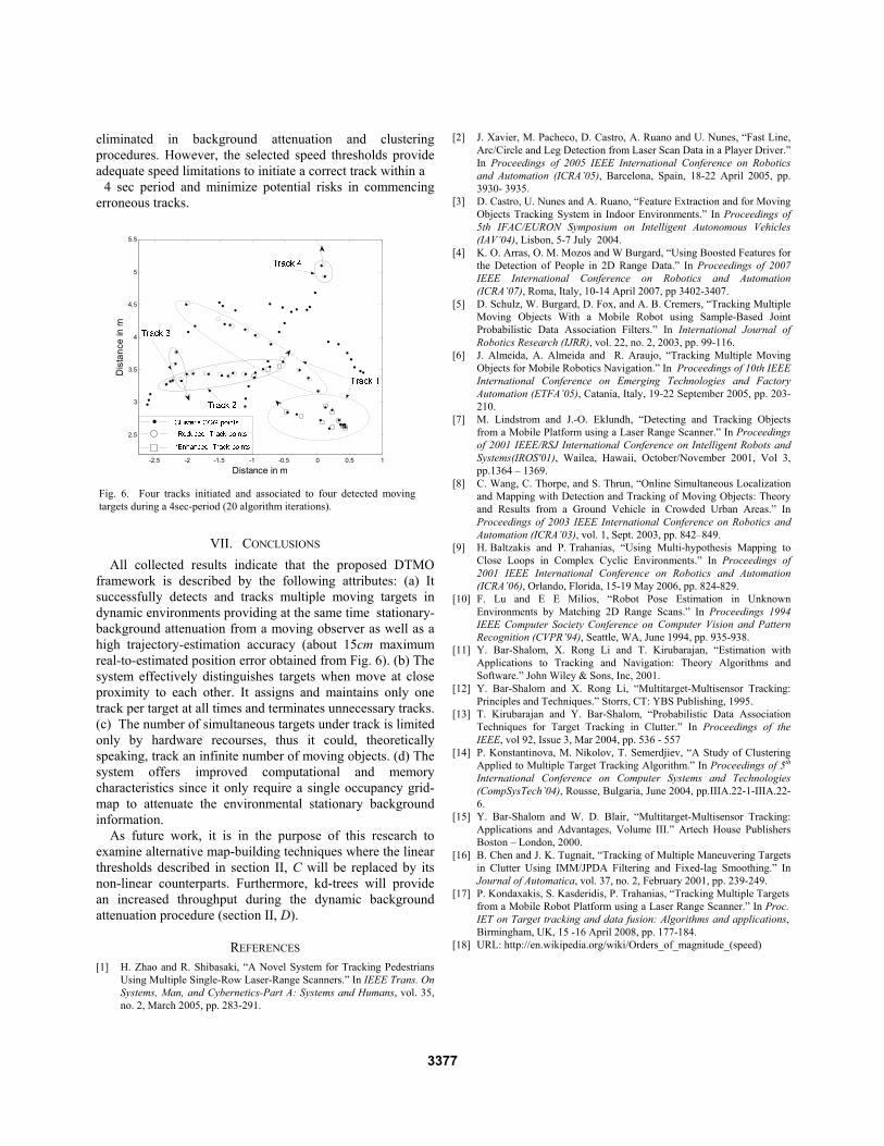
eliminated in background attenuation and clustering procedures. However, the selected speed thresholds provide adequate speed limitations to initiate a correct track within a

4 sec period and minimize potential risks in commencing erroneous tracks.

VII. CONCLUSIONS All collected results indicate that the proposed DTMO

framework is described by the following attributes: (a) It successfully detects and tracks multiple moving targets in dynamic environments providing at the same time stationary-background attenuation from a moving observer as well as a high trajectory-estimation accuracy (about 15cm maximum real-to-estimated position error obtained from Fig. 6). (b) The system effectively distinguishes targets when move at close proximity to each other. It assigns and maintains only one track per target at all times and terminates unnecessary tracks. (c) The number of simultaneous targets under track is limited only by hardware recourses, thus it could, theoretically speaking, track an infinite number of moving objects. (d) The system offers improved computational and memory characteristics since it only require a single occupancy grid-map to attenuate the environmental stationary background information.

As future work, it is in the purpose of this research to examine alternative map-building techniques where the linear thresholds described in section II, C will be replaced by its non-linear counterparts. Furthermore, kd-trees will provide an increased throughput during the dynamic background attenuation procedure (section II, D).

REFERENCES [1] H. Zhao and R. Shibasaki, “A Novel System for Tracking Pedestrians

Using Multiple Single-Row Laser-Range Scanners.” In IEEE Trans. On Systems, Man, and Cybernetics-Part A: Systems and Humans, vol. 35, no. 2, March 2005, pp. 283-291.

[2] J. Xavier, M. Pacheco, D. Castro, A. Ruano and U. Nunes, “Fast Line, Arc/Circle and Leg Detection from Laser Scan Data in a Player Driver.” In Proceedings of 2005 IEEE International Conference on Robotics and Automation (ICRA’05), Barcelona, Spain, 18-22 April 2005, pp. 3930- 3935.

[3] D. Castro, U. Nunes and A. Ruano, “Feature Extraction and for Moving Objects Tracking System in Indoor Environments.” In Proceedings of 5th IFAC/EURON Symposium on Intelligent Autonomous Vehicles (IAV’04), Lisbon, 5-7 July 2004.

[4] K. O. Arras, O. M. Mozos and W Burgard, “Using Boosted Features for the Detection of People in 2D Range Data.” In Proceedings of 2007 IEEE International Conference on Robotics and Automation (ICRA’07), Roma, Italy, 10-14 April 2007, pp 3402-3407.

[5] D. Schulz, W. Burgard, D. Fox, and A. B. Cremers, “Tracking Multiple Moving Objects With a Mobile Robot using Sample-Based Joint Probabilistic Data Association Filters.” In International Journal of Robotics Research (IJRR), vol. 22, no. 2, 2003, pp. 99-116.

[6] J. Almeida, A. Almeida and R. Araujo, “Tracking Multiple Moving Objects for Mobile Robotics Navigation.” In Proceedings of 10th IEEE International Conference on Emerging Technologies and Factory Automation (ETFA’05), Catania, Italy, 19-22 September 2005, pp. 203-210.

[7] M. Lindstrom and J.-O. Eklundh, “Detecting and Tracking Objects from a Mobile Platform using a Laser Range Scanner.” In Proceedings of 2001 IEEE/RSJ International Conference on Intelligent Robots and Systems(IROS'01), Wailea, Hawaii, October/November 2001, Vol 3, pp.1364 – 1369.

[8] C. Wang, C. Thorpe, and S. Thrun, “Online Simultaneous Localization and Mapping with Detection and Tracking of Moving Objects: Theory and Results from a Ground Vehicle in Crowded Urban Areas.” In Proceedings of 2003 IEEE International Conference on Robotics and Automation (ICRA’03), vol. 1, Sept. 2003, pp. 842–849.

[9] H. Baltzakis and P. Trahanias, “Using Multi-hypothesis Mapping to Close Loops in Complex Cyclic Environments.” In Proceedings of 2001 IEEE International Conference on Robotics and Automation (ICRA’06), Orlando, Florida, 15-19 May 2006, pp. 824-829.

[10] F. Lu and E E Milios, “Robot Pose Estimation in Unknown Environments by Matching 2D Range Scans.” In Proceedings 1994 IEEE Computer Society Conference on Computer Vision and Pattern Recognition (CVPR’94), Seattle, WA, June 1994, pp. 935-938.

[11] Y. Bar-Shalom, X. Rong Li and T. Kirubarajan, “Estimation with Applications to Tracking and Navigation: Theory Algorithms and Software.” John Wiley & Sons, Inc, 2001.

[12] Y. Bar-Shalom and X. Rong Li, “Multitarget-Multisensor Tracking: Principles and Techniques.” Storrs, CT: YBS Publishing, 1995.

[13] T. Kirubarajan and Y. Bar-Shalom, “Probabilistic Data Association Techniques for Target Tracking in Clutter.” In Proceedings of the IEEE, vol 92, Issue 3, Mar 2004, pp. 536 - 557

[14] P. Konstantinova, M. Nikolov, T. Semerdjiev, “A Study of Clustering Applied to Multiple Target Tracking Algorithm.” In Proceedings of 5th International Conference on Computer Systems and Technologies (CompSysTech’04), Rousse, Bulgaria, June 2004, pp.IIIA.22-1-IIIA.22-6.

[15] Y. Bar-Shalom and W. D. Blair, “Multitarget-Multisensor Tracking: Applications and Advantages, Volume III.” Artech House Publishers Boston – London, 2000.

[16] B. Chen and J. K. Tugnait, “Tracking of Multiple Maneuvering Targets in Clutter Using IMM/JPDA Filtering and Fixed-lag Smoothing.” In Journal of Automatica, vol. 37, no. 2, February 2001, pp. 239-249.

[17] P. Kondaxakis, S. Kasderidis, P. Trahanias, “Tracking Multiple Targets from a Mobile Robot Platform using a Laser Range Scanner.” In Proc. IET on Target tracking and data fusion: Algorithms and applications, Birmingham, UK, 15 -16 April 2008, pp. 177-184.

[18] URL: http://en.wikipedia.org/wiki/Orders_of_magnitude_(speed)

-2.5 -2 -1.5 -1 -0.5 0 0.5 1

2.5

3

3.5

4

4.5

5

5.5

Dis

tanc

e in

m

Distance in m

Fig. 6. Four tracks initiated and associated to four detected moving targets during a 4sec-period (20 algorithm iterations).

3377