Responses of neurons in the inferior colliculus to binaural disparities: insights from the use of...

A

(a(r(Itwdb©

K

1

nntrttiit1

tJ

0d

Journal of Neuroscience Methods 169 (2008) 391–404

Responses of neurons in the inferior colliculus to binaural disparities:Insights from the use of Fisher information and mutual information

Noam Gordon a, Trevor M. Shackleton b, Alan R. Palmer b, Israel Nelken a,c,∗a Department of Neurobiology, Silberman Institute of Life Sciences, Edmund Safra Campus, Hebrew University,

Givat Ram, Jerusalem 91904, Israelb MRC Institute of Hearing Research, University Park, Nottingham NG7 2RD, UK

c Interdisciplinary Center for Neural Computation, Hebrew University, Jerusalem 91904, Israel

Received 31 July 2007; received in revised form 4 November 2007; accepted 10 November 2007

bstract

The minimal change in a stimulus property that is detectable by neurons has been often quantified using the receiver operating characteristicROC) curve, but recent studies introduced the use of the related Fisher information (FI). Whereas ROC analysis and FI quantify the informationvailable for discriminating between two stimuli, global aspects of the information carried by a neuron are quantified by the mutual informationMI) between stimuli and responses. FI and MI have been shown to be related to each other when FI is large. Here the responses of neuronsecorded in the inferior colliculus of anesthetized guinea pigs in response to ensembles of sounds differing in their interaural time differencesITDs) or binaural correlation (BC) were analyzed. Although the FI is not uniformly large, there are strong relationships between MI and FI.nformation-theoretic measures are used to demonstrate the importance of the non-Poisson statistics of these responses. These neurons may reflect
he maximization of the MI between stimuli and responses under constraints on the coded stimulus range and the range of firing rates. Remarkably,hereas the maximization of MI, in conjunction with the non-Poisson statistics of the spike trains, is enough to create neurons whose ITDiscrimination capabilities are close to the behavioral limits, the same rule does not achieve single-neuron BC discrimination that is as close toehavioral performance. 2007 Elsevier B.V. All rights reserved.
ig; Fis

stqisbMoi

eywords: Auditory system; Binaural disparities; Inferior colliculus; Guinea p

. Introduction

Developing the appropriate tools for the quantification ofeural responses to sensory stimuli is an important goal ineuroscience. Throughout the modern history of neuroscience,he availability of the right quantifiers of stimulus–responseelationships has been crucial for scientific advances. Thus,he study of auditory sensory coding cannot be imaginedoday without tools such as the peristimulus time histogramntroduced by Gerstein (1960), reverse correlation techniques
nitially introduced by De Boer (1968,1969), or the concept ofhe spectro-temporal receptive field (Aertsen and Johannesma,980, 1981; Aertsen et al., 1981).
∗ Corresponding author at: Department of Neurobiology, Silberman Insti-ute of Life Sciences, Edmund Safra Campus, Hebrew University, Givat Ram,erusalem 91904, Israel. Tel.: +972 2 6584229; fax: +972 2 6586077.

E-mail address: [email protected] (I. Nelken).

t

gtappfa

165-0270/$ – see front matter © 2007 Elsevier B.V. All rights reserved.oi:10.1016/j.jneumeth.2007.11.005

her information; Mutual information

While all of the quantifiers above are important for under-tanding how a stimulus affects neuronal responses, a separateoolkit has been developed in order to study the reverseuestion—how can the nervous system use neuronal responsesn order to extract information about the environment. Typically,uch studies start with a set of relevant stimuli (e.g. broad-and noise presented from many different directions in space,iddlebrooks et al., 1994). To evaluate the discrimination based

n single trials, a classifier is trained to use the response recordedn single trials in order to identify the stimulus that gave rise tohe response.

A large number of different classifiers have been used for theeneral problem of classifying neuronal responses. However,his approach is inherently ad hoc: there may always be yetnother, better classifier that will achieve a higher discrimination
erformance based on the same responses. It turns out that theerformance of all classifiers on a given set of responses can inact be uniformly bounded. For this purpose, the performance ofclassifier is quantified by the so-called transmitted information.
mailto:[email protected]

dx.doi.org/10.1016/j.jneumeth.2007.11.005

3 scien

Tmsoirtp2

cttrhutTcctc

taFrctipulTageo2

inopacrad(

ote

t‘

utnco

2

2

Drie(

ttmLstfi

D2fiKStwSoa

ftscwtsoiF

trotvalue). Data was sometimes collected for a number of different

92 N. Gordon et al. / Journal of Neuro

he transmitted information is computed from the confusionatrix, which estimates how many times a response to a given

timulus was classified as resulting from the presentation of anyf the other stimuli. The transmitted information of any classifiers bounded by the mutual information (MI) between stimuli andesponses, a measure that can be computed without any referenceo a specific classifier. Thus, the MI is an absolute bound on theerformance of any classifier (see the review in Nelken et al.,005).

One important special case occurs often in the literature. Inase the set of relevant stimuli consists of only two stimuli,he classifier becomes a discriminator whose goal is to iden-ify which of the two stimuli was presented given single trialesponses. In the context of the auditory system, this approachas been extensively applied to the case in which the two stim-li are close to each other along some sensory scale, leadingo estimates of the sensory resolution of single trial responses.he tool that has been traditionally used for quantifying the dis-rimination between pairs of stimuli is the receiver operatingharacteristic (ROC) curve. This curve can be used to estimatehe best possible performance in a 2-alternative, 2-interval forcedhoice task (Green and Swets, 1966).

When testing the sensory resolution, so that the two stimulio be discriminated are very similar to each other, there is anlternative measure of performance: the Fisher information (FI).I is a sensitivity measure: it measures the extent by which theesponse of the neuron changes when the sensory parameter ishanged by a small amount (Schervish, 1995). Clearly, whenhe response is a sensitive function of the sensory parameter,t will be easier to discriminate between nearby values of thatarameter. The main importance of FI is the fact that it can besed to extrapolate single-neuron discrimination capabilities toarge populations, which is difficult to do with ROC analysis.hus, when they make sense and can be estimated, FI and MIre in fact appealing quantifiers of neural responses. FI in variousuises has been used for a long time (e.g. Siebert, 1965), but itsxplicit use in auditory research is to the best of our knowledgenly rather recent (Harper and McAlpine, 2004; Heinz et al.,001a,b; Jenison, 2000; Jenison and Reale, 2003).

Since ROC curves, FI and MI are different measures of thenformation that is available in single neuronal responses, it isatural to ask what the relationships between them are. The the-retical relationships will be discussed in Section 2. The firsturpose of this paper is to compare these relationships withctual measured responses. The data consist of a previouslyollected, unique set of responses of inferior colliculus (IC) neu-ons in guinea pigs (Shackleton et al., 2003, 2005; Skottun etl., 2001) to two types of binaural disparities: interaural timeifferences (ITDs) and various levels of binaural correlationBC).

The neurons were studied with an extremely high-resolutionf the sensory continua, and each ITD or BC value wasested ≥ 100 times. This makes the dataset large enough to stably
stimate all three information measures.
The second purpose of this paper is to illustrate the impor-ance of information-theoretic measures for understanding thedesign features’ of neurons. Information-theoretic measures are

fetb

ce Methods 169 (2008) 391–404

sed to demonstrate the importance of the non-Poisson statis-ics of the responses of these neurons, and to suggest that theseeurons optimize the MI between stimuli and responses underonstraints on the range of the encoded parameters and the rangef firing rates.

. Methods

.1. Electrophysiology

The paper is based on the data from Shackleton et al. (2005).etailed methods are described in the above paper. In short,

esponses of well-separated single neurons were collected in thenferior colliculus (IC) of urethane-anesthetized guinea pigs. Allxperiments were carried out in accordance with the UK AnimalScientific Procedures) Act of 1986.

Stimuli were delivered to each ear through sealed acous-ic systems comprising custom-modified Radioshack 40-1377weeters joined via a conical section to a damped 2.5-

m-diameter, 34-mm-long tube (M. Ravicz, Eaton Peabodyaboratory, Boston, MA, USA), which fitted into the hollowpeculum. The output was calibrated a few millimeters from theympanic membrane using a Bruel and Kjær 4134 microphonetted with a calibrated 1-mm probe tube.

All stimuli were digitally synthesized (System II, Tucker-avies Technologies) at sampling rates between 100 and00 kHz and were output through a waveform reconstructionlter set at one fourth the sampling rate (135 dB/octave elliptic:emo 1608/500/01 modules supported by custom electronics).timuli were of 50-ms duration at 20 dB above the threshold for

hat stimulus, switched on and off simultaneously in the two earsith cosine-squared gates with 2 ms rise/fall times (10–90%).ince gating was applied simultaneously in both ears, there werenly ongoing interaural phase differences (IPDs) in the stimulusnd no onset ITD.

The stimuli consisted of narrow noise bands around the bestrequency of each neuron (one equivalent rectangular band forhe guinea pig, about 6.477f0.56 at center frequency f kHz). Thetimuli were presented with varying ITD or varying binauralorrelation (BC). For the ITD responses, 16–31 ITD valuesere selected at a typical resolution of 0.01 cycles covering

he dynamic range of the neuron. For BC variation only noisetimuli were used. The stimuli were presented at the best ITDf the neuron. BC varied from −1 to 1 in steps of 0.1 (21 valuesn all). Examples of stimuli with different BC are displayed inig. 1A.

Data was acquired only from neurons with good modula-ion of the rate by interaural delay and a spike signal-to-noiseatio that was judged likely to be sufficient for a recordingf 2–3 h. The noise stimuli were ‘frozen’ (the same stimulusoken was presented for all presentations of each ITD or BC

rozen tokens of the noise stimuli. Only in a few cases differ-ntial sensitivity to the noise tokens was found, and thereforehe responses to all tokens were superimposed in the analyseselow.

N. Gordon et al. / Journal of Neuroscience Methods 169 (2008) 391–404 393

Fig. 1. (A) The stimuli presented to the left and right ears for producing BC = −0.7 (left) and BC = 0.7 (right) for one neuron. (B) The resulting spike countdistributions. White bars: distribution of spike counts when presenting the stimulus with BC = −0.7. Black bars: distribution of spike counts when presenting thestimulus with BC = 0.7. The value above each bar represents the ratio between the two probabilities (the likelihood). (C) The joint distribution of stimuli and responsesfor the same neuron. The abscissa represents BC, the ordinate represents the spike counts, and the gray level represents the probability. The spike count distributionsfrom (B), scaled by the probability of observing a stimulus (1/21 in this case) are marked by the arrows. (D) Probability of correct discrimination between BC = 0.7and all other tested BC values for this neuron, computed using ROC analysis. The gray line represents a discrimination performance of 75%. (E) FI as a function ofB rdinata s.

2

sttmp

jhuθ

obFt

absitatrpsttr

C (black line, left ordinate) and the JND estimated from FI (gray line, right obout 0.3 correlation units, very close to the value estimated from ROC analysi

.2. Information calculations

For simplicity, the responses are quantified by the evokedpike counts, ignoring the exact timing of the action poten-ials. The general issue studied here is therefore how to identifyhe stimulus based on the spike count it evoked. The perfor-

ance of single neurons is considered here rather than that ofopulations.

The calculation of all information measures is based on theoint distribution of stimuli and responses. In the case treatedere, this is the distribution of spike counts for each of the stim-li presented in the experiment. For a stimulus with parameter(representing either ITD or BC), the probability distribution

f the counts is denoted by P(x|θ). Two examples of such distri-utions, in response to the stimuli in Fig. 1A, are illustrated inig. 1B. The joint distribution of stimuli and responses reflects

he probability of observing a response given a stimulus, but

astf

e; expressed in correlation units) for the same neuron. The JND at BC = 0.7 is

lso the probability of presentation of each stimulus. It is giveny P(x|θ)P(θ), where P(θ) is the probability of presenting atimulus θ. In most experiments, P(θ) is just 1/N, where Ns the total number of different stimuli that are used. Ratherhan assuming a parametric form for these distributions, theyre estimated here from the data. Fig. 1C shows the joint dis-ribution of stimuli and responses for the same neuron whoseesponses are illustrated in Fig. 1B. The two distributions dis-layed in Fig. 1B form part of this joint distribution, aftercaling by the number of stimuli, 21 in this case. As a cau-ionary note, all information measures (including ROC analysis)hat use the estimated joint distribution of stimuli and responsesequire large amounts of data in order to avoid the biases that
re inherent in these calculations. Calculating these values forparsely sampled joint distribution produces estimates that areypically far too large (see Nelken et al., 2005; Paninski, 2003or details).

3 scien

2

((wr

ridoet

sssctrctoiwctss

totpsSbttwttrmBcfldtdwoo

ie

ttttermTgrec

idtpibrFo7oco

2

bIfnoθ

capt

F

Fr(Fp

Cpθ

function θ = θ(x) of the neuronal responses (spike counts in our


.2.1. ROC analysisWe repeated the ROC analysis performed by Shackleton et al.

2003, 2005) on the same data. For every pair of parameter valuesITD or BC), the two observed distributions of spike countsere used for evaluating the performance of an optimal decision

ule.In ROC analysis, a decision rule based on the single trial

esponses is used to discriminate between the two stimuli. Sincet is assumed that all decisions are based on spike counts, aecision rule simply consists of assigning each possible valuef the spike counts to one of the two stimuli. The decision onach trial is then based on the spike count observed in thatrial.

Although the situation is symmetric with respect to the twotimuli, the terminology is not. One of the two stimuli is con-idered as a reference stimulus and the other one as the targettimulus. When observing a trial of the reference stimulus, aorrect decision is reached if the observed spike count belongso the set of spike counts assigned by the decision rule to theeference stimulus, and an error occurs if the observed spikeount belongs to the set of counts assigned by the decision ruleo the target stimulus. The probability of making an error whenbserving a trial of the reference stimulus is called the probabil-ty of false alarms or false positives. Similarly, when presentedith a trial coming from the target stimulus, the rule makes a

orrect decision if the observed spike count is assigned to thearget stimulus; otherwise it makes an error. The correct deci-ions, when presented with a trial from the target stimulus, areometimes called ‘correct detections’.

Up to this point, the decision rule was not specified. Byhe lemma of Neyman and Pearson (Lehman, 1986, p. 72),ptimal decision rules are based on the likelihood—the ratio ofhe probabilities for observing each possible spike count whenresented with the target and the reference stimuli. Fig. 1Bhows the likelihood for the two probability distributions.pike counts are assigned to the reference or target stimuliy setting a threshold on the likelihood function. For eachhreshold, those spike counts whose likelihood is larger than thehreshold are assigned to the target stimulus and spike countshose likelihood is smaller than the threshold are assigned

o the reference stimulus. For example, in Fig. 1B, when thehreshold is 1, trials with 0, 1 or 2 spikes would be classified asesulting from stimuli with BC = −0.7, whereas trials with 3 orore spikes would be classified as resulting from stimuli withC = 0.7. Clearly, a very high threshold results in a low rate oforrect detections and a low rate of false alarms, since only aew possible spike counts are assigned to the target stimulus;owering the threshold increases both false alarms and correctetections. When the threshold is 0, all likelihoods are abovehreshold and all trials are classified as belonging to the targetistribution, resulting in certainty of correct detection but alsoith a similar certainty of false alarms. The ROC curve is a plotf the probability of correct detections against the probabilityf false alarms for all of these decision rules.

In most applications of ROC analysis to neural data (notably,n the previous analyses of the data considered here, Shackletont al., 2005), the threshold has been set on spike counts rather

cnt

ce Methods 169 (2008) 391–404

han on likelihoods: all spike counts that are larger than thehreshold are assigned to one class and all spike counts smallerhan the threshold are assigned to the other class, depending onhe relative size of the mean response to each stimulus. How-ver, such rules are not necessarily optimal. Basing the decisionule on thresholding spike counts is optimal only if there is aonotonic relationship between likelihoods and spike counts.his is true for Poisson distributions (for example), but not foreneral probability distributions. Here only the optimal decisionules based on likelihood were used. Their performance was, asxpected, always better than rules based on thresholding spikeounts, although the differences were not large.

The area under the ROC is the probability of correct decisionn a 2-alternative, 2-interval forced choice task based on theseistributions. Thus, it is possible to use the ROC analysis in ordero get estimates of the just-noticeable difference (JND). For eacharameter value, the JND is considered as the smallest differencen parameter value that resulted in a discrimination probabilityetter than 75%, which corresponds to the probability of correctesponses that is usually tracked in psychophysical experiments.ig. 1D shows the probability of discrimination between a BCf 0.7 and all other BCs. The gray lines represent the criterion of5% correct discriminations. Using spike counts in single trialsf this neuron, it is possible to discriminate between binauralorrelations of 0.7 and 0.4, so that the JND of this neuron at BCf 0.7 is 0.3 correlation units.

.2.2. Fisher informationFI is defined for families of probability distributions indexed

y a continuous variable θ. In the data analyzed here, θ representsTD or BC, as discussed above. In order to use the spike countsor discriminating between two nearby ITDs, it is obviouslyecessary for some spike counts to be typical for one ITD, andther spike counts to be typical for the other ITD. Thus, changingshould increase the probability of seeing some possible spike

ounts and reduce the probability of seeing other counts. FI isfunction of the parameter θ that quantifies this change in therobability distribution of the possible neuronal responses dueo a small change in θ.

The FI is defined as (Lehman, 1983, p. 118)

I(θ) =EQ

[∂ log(P(x|θ))

∂θ

]2

=∑

x

P(x|θ)

[∂ log(P(x|θ))

∂θ

]2

(1)

I is additive: the FI for many statistically independent neu-ons would be the sum of the FIs of each individual neuronLehman, 1983, p. 121). Thus, it is a simple matter to move fromI calculated for a single-neuron to the FI of a large neuronalopulation.

The importance of the FI for our purpose stems from theramer–Rao bound (Lehman, 1983, p. 122), which makes itossible to translate FI into an estimate of the JND. Very often,has to be estimated from the neuronal responses, that is, a

ase) is required that will approximate θ as well as possible. Aatural (but not necessary) requirement on such a function iso be unbiased. This means that its average, over all possible

rosci

r

E

(fs

v

wt

idcddc

b(

aItc

TultiisiF

pcrpsffs

pptod

set

cwaaia2prwcnoePwolbbao

2

tomtta

M

wxtt

inrbtpotp

N. Gordon et al. / Journal of Neu

esponses to stimuli with parameter θ, should be equal to θ:

θθ =∑

x

P(x|θ)θ(x) = θ.

The Cramer–Rao bound states that under these conditionsand under some technical conditions that would generally holdor neural data), the variance of the estimates of θ can be nomaller than the inverse of the FI:

arθ�

θ ≥ 1

FI(θ)

here the variance is taken with respect to the possible responseso stimuli with parameter θ.

Assuming that two values of the parameter θ are discrim-nable when they are separated by more than one standardeviation of the estimator, it is possible to translate the FI into aorresponding JND: the JND will be the width of the expectedistribution of the estimator, which is measured by its standardeviation. Thus, the FI corresponds to JNDs which are about/√

FI(θ), where the constant c may depend on the exact distri-ution of spike counts. For the data analyzed here, c is about 2see below).

FI can be considered as a ‘figure of merit’ for an ROCnalysis performed on the responses to two close values of θ.ndeed, when the parameter θ changes by a small amount �θ,he change in the likelihood ratio for a given observed spikeount x is

P(x|θ+�θ)−P(x|θ)

P(x|θ)≈ (∂P(x|θ)/∂θ)�θ

P(x|θ)

=(

∂ log(P(x|θ))

∂θ

)�θ.

he larger this change is, the more discriminable the two stim-li when the spike count x is observed. Since the change inikelihood can be both positive and negative, it is squaredo ensure that it is always positive. To combine the changesn the likelihood ratio at all possible observed spike countsnto an overall figure of merit, it is reasonable to weigh thisquared change in likelihood ratio by the probability of observ-ng the specific spike count x. This is precisely the definition ofI.

Although in essentially all applications of FI (and in thisaper as well) neural responses are quantified by the total spikeount, FI can be computed for other measures of the neuronalesponses. As an extreme example, with enough data, it may beossible to estimate the probabilities of observing all possiblepike patterns in the data. These probabilities will again be aunction of the parameter θ, and the FI can be computed for thisamily of probability distributions exactly as it is calculated forpike count distributions.

Calculating FI requires estimating of the derivative of therobability distribution. In practice, this requires estimating the
robability P(x|θ) for two nearby values of θ and then takinghe difference between the two estimates. Since the estimatesf P(x|θ) for low-probability spike counts x may be noisy, theifferences are also noisy. Furthermore, since the derivatives are
toit

ence Methods 169 (2008) 391–404 395

quared before averaging, these errors add up rather than cancelach other. Thus, the FI estimated directly with Eq. (1) willypically be too large.

Before applying Eq. (1), pre-processing included (i) zeroorrection—bins of 0 were increased to 1/3 counts, bins thatere equal to 1% of the total counts or more were not adjusted,

nd bins that had between 0% and 1% of the total counts weredjusted by a proportionally smaller amount; and (ii) smooth-ng, using a smoothing spline (a smooth cubic spline minimizing

weighted sum of the fit error and of the magnitude of thend derivative, using the Matlab routine csaps; the smoothingarameter was around 0.6). These parameters produced the bestesults when using data simulated from Poisson distributions, forhich FI can be computed analytically. The simulated datasets

onsisted of the same number of trials as collected for a typicaleuron, and the range of firing rates was set to the typical valuesbserved in the data. Smoothing was performed separately forach value of spike count, producing a smoothed estimate of(x|θ) as a function of θ. The derivative of the smoothing splineas used for calculating FI. The black line in Fig. 1E is a plotf FI(θ) for the spike count distributions in Fig. 1C. The grayine (corresponding to the right scale) is the estimate of the JNDased on FI, 2/

√FI(θ). For this neuron, the best JND estimate

ased on the FI is remarkably similar to that based on the ROCnalysis: about 0.3 correlation units for a reference correlationf 0.7.

.2.3. Mutual informationIn contrast to ROC analysis and FI, which are local in

he sense that they consider each individual value (or pairsf values) of the sensory variable separately, mutual infor-ation (MI) is a global measure for the performance of

he neuron. The MI depends on the joint probability dis-ribution of stimuli and responses, P(x, θ). It is defineds

I =∑

P(x, θ)log2

(P(x, θ)

P(x)P(θ)

),

here P(x) is the overall probability of observing the spike count(across all stimulus presentations, averaged over stimulus iden-

ity), and P(θ) is as usual the overall probability of the stimuluso have the parameter θ.

MI measures the expected reduction in uncertainty in thedentity of the stimulus due to the observation of a singleeuronal response. Before observing the response of the neu-on, the best guess regarding the identity of the stimulus isased on the overall distribution of stimuli. For example, inhe dataset analyzed here, all stimuli occurred with the samerobability. The uncertainty in this case is maximal—beforebserving a response, there is not any reason to preferen-ially guess one stimulus rather than another one. For theurpose of calculating MI, the uncertainty in the identity of
he stimulus is quantified by the entropy of the distributionf stimuli. This entropy in the case of N equiprobable stimulis log2N, which is the maximum possible entropy for a dis-ribution of N possible stimuli. At the other extreme, if one

3 scien

sne

slsBsioOctrbsarbcuote

awr(esiusdsb

secs

i(tbatdmtptii

wd

(i

M

w(m(booismpcMtawmwBro

2

trRbotTttbgh

mrptor


timulus is certain to be presented and all other stimuli can-ot occur, the entropy is 0. This entropy is called the a-priorintropy.

Following the observation of a single neuronal response,ome stimuli may become more probable and other may becomeess probable. For example, a large spike count may be con-istent with contralateral ITDs but not with ipsilateral ones.ayes rule makes it possible to calculate the probability of each

timulus given the observed response of the neuron, produc-ng a new probability distribution: the probability distributionf the stimuli conditioned on observing a specific spike count.bviously, such a conditional probability distribution can be

omputed for each possible value of the spike count. Each ofhese distributions has its own entropy: if the observed responseesults in a small number of stimuli that are highly proba-le while all other stimuli are improbable, the entropy will bemall. If, on the other hand, the observed response results inpproximately equal probability for all stimuli, the entropy willemain large. The average of these entropy values (weightedy the probability of each observed spike count) is called theonditional entropy. The conditional entropy is the averagencertainty in the identity of the stimulus that remains afterbserving the response in a single trial. The MI turns out to behe difference between the a-priori entropy and the conditionalntropy.

If the stimulus that was presented can be identified correctlyfter the observation of a single trial, the conditional entropyill be 0 and the MI will be equal to the a-priori entropy. This

equires each spike count to occur in response to a single stimulusalthough a stimulus can still give rise to a number of differ-nt spike counts). When this happens, the uncertainty in thetimulus is reduced to 0. On the other hand, if the response isndependent of the stimuli, the probability of the stimuli will benaffected by the observation of a response, and the conditionaltimulus distributions will be the same as the a-priori stimulusistribution. As a result, the conditional entropy will be equal totimulus entropy and the MI, the difference between them, wille 0.

Thus, the MI has an absolute scale: if 0, the responses do notupply any information about the stimulus, while if the MI isqual to stimulus entropy (which it cannot exceed), the stimulusan be identified with certainty based on the observation of aingle trial.

The MI has a number of properties that makes it an appeal-ng candidate for quantifying stimulus–response relationshipsNelken and Chechik, 2007). In particular, the so-called informa-ion processing inequality states that the MI cannot be increasedy any processing performed on the responses. Consider nowdecoder that guesses the identity of the stimulus based on

he observation of single-trial responses. The guess that theecoder produces is a function of the response. The confusionatrix can therefore be considered as the joint distribution of

he stimuli and a function of the responses, namely the guesses
roduced by the decoder. Furthermore, the so-called transmit-ed information is the MI of the confusion matrix. Thus, by thenformation processing inequality, the transmitted informations bounded by the MI between stimuli and responses. In other
teaw

ce Methods 169 (2008) 391–404

ords, the MI is an absolute bound on the performance of anyecoder.

The MI was estimated using the ‘adaptive direct’ methodNelken and Chechik, 2007; Nelken et al., 2005). The MI wasnitially calculated using the naıve estimator,

I =∑ϑ,x

P(x, θ) log

(P(x, θ)

P(x)P(θ)

),

here P(x, θ) was estimated as P(x|θ)P(θ) with P(θ) = 1/NN was the number of different stimuli). The naıve esti-ator may be biased, and the bias was estimated as

N − 1) (#x − 1)/(2Tlog(2)), where #x is the number of possi-le response values, and T is the total number of trials (summedver all stimuli). Next the matrix was reduced by adding the rowr column with the smallest number of measurements to that ofts immediate neighbors that had the smaller number of mea-urements. The MI and bias of this reduced joint distributionatrix were estimated, and the matrix was reduced again. This

rocess was repeated until the matrix collapsed to a single row orolumn. The process resulted in a decreasing sequence of naıveI values and a decreasing sequence of bias values. However,

he corrected MI, which is the difference between the naıve MInd the corresponding bias, often had a non-monotonic behaviorith an initial increase followed by a decrease. The MI was esti-ated as the maximum bias-corrected MI, where the maximumas taken over all reduced matrices generated by the process.ecause of the large number of stimulus repetitions, the bias

epresented only a small fraction (<10%, very often much less)f the typical raw MI.

.2.4. Relationships between ROC analysis, FI and MIROC analysis and FI can both be used to estimate the JND in

he sensory parameter after the observation of a single neuronalesponse. Theoretically, there is no reason for the JND based onOC analysis to be larger or smaller than the estimate of the JNDased on the FI. On the one hand, FI bounds the performancef unbiased estimators, whereas the decision rules underlyinghe ROC curve are not limited to the use of unbiased estimators.herefore, the JND based on ROC analysis may be smaller than

hat based on FI (and this will be apparent in the data below). Onhe other hand, FI is a lower bound which may not be reachabley any means. Therefore, it may represent an unrealisticallyood discrimination performance although this did not seem toappen in the data analyzed here.

The relationships between MI and FI or ROC analysis areore complex. Given a high-resolution measurement of the

esponses of a neuron to a sensory parameter (ITD or BC), it isossible to characterize the overall performance of the neuron byhe MI. It is also possible to characterize the overall performancef the neuron by average FI. Are these two characterizationselated to each other, and if so, how?

Fig. 2 shows a schematic representation of this situation, and
he expected relationship between MI and FI. The MI is consid-red as the reduction in uncertainty following the observation ofsingle neuronal response. If the range of θ is N, stimulus entropyill be proportional to log2N. After observing a response, the


Fd

vataawtt

b2iaiit

3

3c

apeecatcnr

ctKT2n(nb

Fig. 3. (A) Rate-ITD function (black line) and rate-BC function (gray line) forone neuron. The abscissa represents the interaural phase difference (in cycles)and the binaural correlation. The ordinate is expressed in spikes/trial. (B) Distri-bution of coded IPD ranges for all neurons in the sample (see text for definitionof the coded range). The arrow represents the expected coded range for cross-correlation of half-wave rectified sine wave, which is the standard model for thercc

awBfi

tItBabBtrtsiB

ig. 2. Relationships between MI and FI at the limit of large FI (see text foretails).

alue of θ can be estimated up to a standard deviation ofpproximately c/

√FI(θ). In Fig. 2 (middle), two conditional dis-

ributions, each conditioned on observing a different spike count,re illustrated schematically. Thus, the entropy after observingresponse should be proportional to log2(c/

√FI(θ)). The MI,

hich is the reduction in uncertainty due to the observation ofhe response, is just the difference between stimulus entropy andhe average conditional entropy (Fig. 2, bottom).

This rough estimate has been made more precise by a num-er of authors (Brunel and Nadal, 1998; Kang and Sompolinsky,001). For specific assumptions about the distributions involved,t is possible to prove that such a relationship will hold when theverage FI is large (so that the conditional entropy is small). Thiss however not the situation with typical single-neuron record-ngs in sensory systems: while the maximal FI may be large, theypical FI for any single-neuron will be small (see below).

. Results

.1. Coding of interaural time differences and binauralorrelation

Although even neurons in the first central station of theuditory system, the cochlear nucleus, may respond to soundsresented to either ear (Davis, 2005; Ingham et al., 2006; Shoret al., 2003; Sumner et al., 2005), fine binaural disparities are firstxtracted in the superior olive. Low-frequency sounds are pro-essed in the medial superior olive (MSO), where an operationkin to cross-correlation is performed. These neurons projecto the inferior colliculus, where their responses are further pro-essed. Fig. 3A shows the responses of an IC neuron to a narrowoise band with varying ITDs that were selected to span its fullange of firing rates (black line).

The fact that ITD is computed by a mechanism approximatingross-correlation in MSO causes neurons in MSO (and theirargets in IC) to be sensitive to changes in BC as well (Albeck andonishi, 1995; Coffey et al., 2006; Joris et al., 2006; Keller andakahashi, 1996; Palmer et al., 1999; Shackleton and Palmer,006; Yin et al., 1987). Fig. 3A shows the responses of the same
euron to narrow noise bands with BC varying from −1 to 1gray line). These stimuli were shifted to the best ITD of thiseuron. The sensitivity to BC was generally monotonic, withest responses most often at a BC of 1 and worst responses at
drr

esponses of MSO neurons which serve as input to the IC. (C) Distribution ofoded BC range for all neurons in the sample. The arrow represents the expectedoded range as calculated by Albeck and Konishi (1995).

BC of −1. The shape of this monotonic relationship varied,ith some neurons reaching their lowest responses already at aC close to 0, while others showing a further decrease of theirring rate even for negative BCs.

The maximal and minimal responses to the ITD and BC con-inua are closely related. Since the stimuli were presented at bestTD, the stimulus with BC = 1 is identical to the stimulus used athe peak of the ITD function. On the other hand, a stimulus withC = −1 is similar to the stimulus used to evoke the responset worst ITD (e.g. Shackleton and Palmer, 2006, the differenceetween the stimuli evoking minimal responses for the ITD andC experiments stems from the use of narrow noise bands rather

han pure tones, so that inverting the stimulus to achieve a cor-elation of −1 is not equivalent to any shift in time). As a result,he responses of a given neuron to ITD and to BC are expected topan approximately the same range of spike counts (as illustratedn Fig. 3A). The firing rate as a function of ITD (respectivelyC) will be denoted by rITD and rBC.

To further quantify the rate functions, the coded range wasefined as the parameter range (ITD or BC) over which the firingate of the neurons changed from 10% to 90% of their responseange (the difference between minimal and maximal responses).

3 scien

soqccoTdectn

poarTt(0ena

w(pscoi

threosbb

3

n(aFavTtmfsFnirt

Fp(


Fig. 3B shows a histogram of the coded ranges for the neuronstudied here, expressed as interaural phase differences (IPDs) inrder to be comparable between neurons with different best fre-uencies. These ranges should be compared with the expectedoded range. It was computed as the rising phase of the auto-orrelation of a half-wave rectified sine wave (the expectedperation performed at the MSO), which is about 0.26 cycles.he IPD ranges were mostly smaller than this—the peak of theistribution is at about half this range. Thus, the range of IPDsncoded by IC neurons is narrower than expected from the cross-orrelation of half-wave rectified responses. The narrowing ofhe coded range could be at least partially due to properties ofeurons in the cochlear nucleus (Louage et al., 2006).

The maximal ITD that would be encountered by a guineaig in nature is about 180 �s, corresponding to an IPD changef 0.09 cycles at 500 Hz and 0.18 cycles at 1000 Hz. Thus, thectual coded IPD range of IC neurons fits better the ethologicalange of ITDs than expected by a naıve cross-correlation model.here is a weak, but non-significant, tendency for the IPD ranges

o be somewhat higher for neurons whose BF is above 500 Hzbelow 500 Hz: IPD range 0.16 ± 0.06, n = 22; above 500 Hz:.21 ± 0.08, n = 8). This tendency is consistent with the hypoth-sis that the narrowing of the coded ranges is an attempt to fit theeuronal ranges with the ranges of ITDs actually encountered,lthough more data is required to support this claim.

For the rBC function, computing the expected range is some-hat more involved. Using the approach of Albeck and Konishi

1995), the ‘default’ rBC function was considered as beingroportional to the binaural correlation between white noise pre-
ented to the two ears at the given BC, after being filtered by aritical band filter in each ear. Using their calculation, the rangef BC values over which the rate increases from 10% to 90%s about 1.3 correlation units. Fig. 3C shows the histogram of
aRec

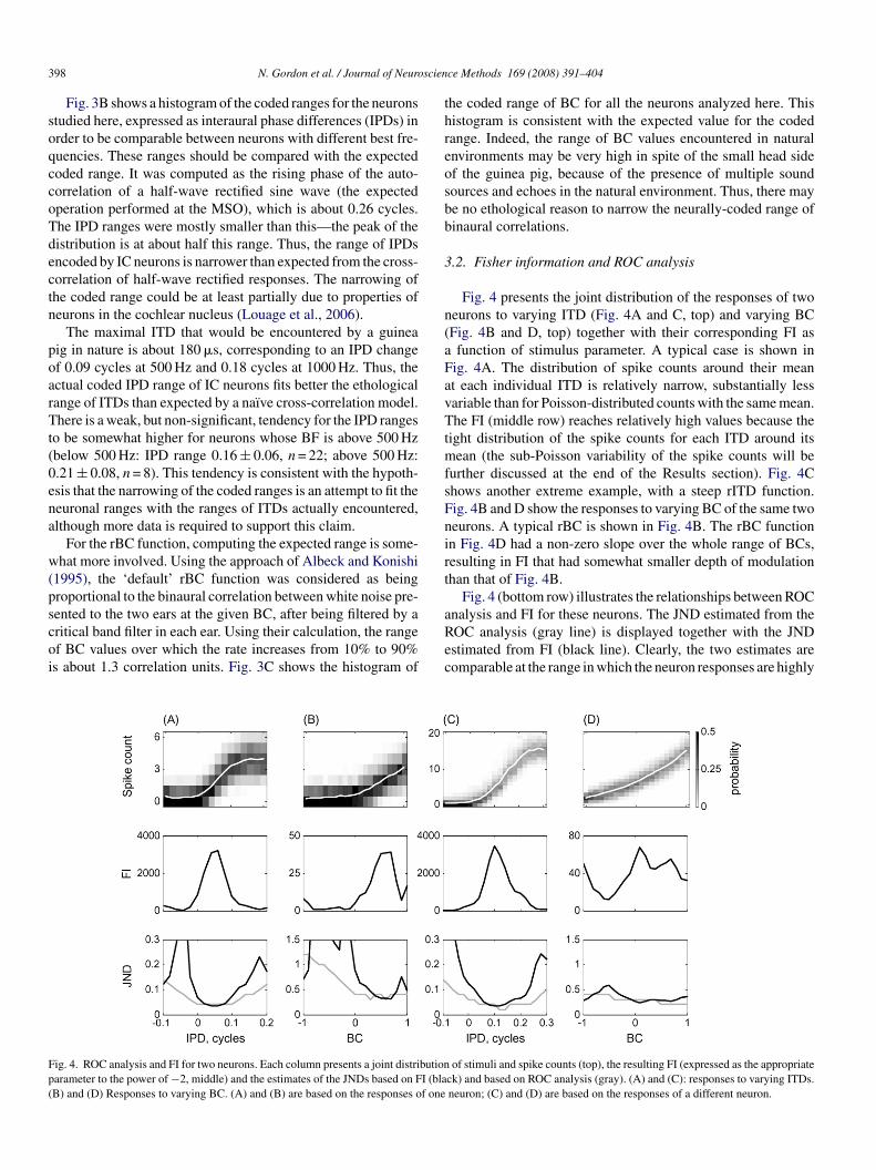
ig. 4. ROC analysis and FI for two neurons. Each column presents a joint distributionarameter to the power of −2, middle) and the estimates of the JNDs based on FI (blaB) and (D) Responses to varying BC. (A) and (B) are based on the responses of one

ce Methods 169 (2008) 391–404

he coded range of BC for all the neurons analyzed here. Thisistogram is consistent with the expected value for the codedange. Indeed, the range of BC values encountered in naturalnvironments may be very high in spite of the small head sidef the guinea pig, because of the presence of multiple soundources and echoes in the natural environment. Thus, there maye no ethological reason to narrow the neurally-coded range ofinaural correlations.

.2. Fisher information and ROC analysis

Fig. 4 presents the joint distribution of the responses of twoeurons to varying ITD (Fig. 4A and C, top) and varying BCFig. 4B and D, top) together with their corresponding FI asfunction of stimulus parameter. A typical case is shown in

ig. 4A. The distribution of spike counts around their meant each individual ITD is relatively narrow, substantially lessariable than for Poisson-distributed counts with the same mean.he FI (middle row) reaches relatively high values because the

ight distribution of the spike counts for each ITD around itsean (the sub-Poisson variability of the spike counts will be

urther discussed at the end of the Results section). Fig. 4Chows another extreme example, with a steep rITD function.ig. 4B and D show the responses to varying BC of the same twoeurons. A typical rBC is shown in Fig. 4B. The rBC functionn Fig. 4D had a non-zero slope over the whole range of BCs,esulting in FI that had somewhat smaller depth of modulationhan that of Fig. 4B.

Fig. 4 (bottom row) illustrates the relationships between ROC
nalysis and FI for these neurons. The JND estimated from theOC analysis (gray line) is displayed together with the JNDstimated from FI (black line). Clearly, the two estimates areomparable at the range in which the neuron responses are highly
of stimuli and spike counts (top), the resulting FI (expressed as the appropriateck) and based on ROC analysis (gray). (A) and (C): responses to varying ITDs.neuron; (C) and (D) are based on the responses of a different neuron.


Fig. 5. (A) Scatter plots of best JNDs for ITD estimated from ROC analysis(abscissa) and FI (ordinate). JNDs are expressed in fraction of a cycle. (B)Scatter plots of the best JNDs for BC estimated from ROC analysis (abscissa)aaa

stat

taftradtnnws

aaypw

3

wsss

Fig. 6. (A) The distributions of MI for ITD and BC, expressed as box plots.The middle of each box represents the median of the distribution. The upperand lower edges of the box are the 25% and 75% values of the distribution.The + signs represents outliers. (B) The distributions of MI for ITD and BC,after normalization by stimulus entropy. These values are bounded between 0(no information) and 1 (maximal information, leading to perfect discriminationperformance). (C) Scatter plots of the MI estimated for ITD (abscissa) and BC(ordinate) for all neurons in the sample. (D) Same for the MI normalized bys

ve

nd1tprbBpttbp

iclt‘

ttec

nd FI (ordinate). JNDs are expressed in correlation units. (C) Scatter plots ofll JND estimates (at all ITDs and all neurons) from ROC analysis (abscissa)nd FI ordinate. (D) Same as (C), for BC.

ensitive to ITD (or BC). On the other hand, above and belowhe sensitive range of the neuron, the JNDs based on the ROCnalysis were almost always smaller than those estimated fromhe FI.

Fig. 5A and B display the scatter plot of the best JND fromhe FI calculations versus the best JND derived from the ROCnalysis, for all neurons, separately for the ITD responses andor the BC responses. The best JNDs from the ROC analysisended to be comparable to the estimates based on FI. The cor-elations between the two estimates of JND were 0.55 (Fig. 5A)nd 0.86 (Fig. 5B). These correlations are highly significantlyifferent from 0. In addition, the two estimates of the JNDended to scatter around the diagonal and did not differ sig-ificantly from each other (paired t-test, ITD: t = 0.7, d.f. = 29,.s.; BC: t = 2, d.f. = 29, n.s.). Similarly, the parameter values athich the best JNDs were found were highly correlated (data not

hown).Fig. 5C and D show the scatter plot of all JND estimates, for

ll tested ITDs and all neurons. The JNDs estimated from FIre on average larger than those estimated from the ROC anal-sis (ITD: t = 10.3, d.f. = 545, p � 0.05; BC: t = 8.3, d.f. = 592,� 0.05), showing that the behavior of the neurons in Fig. 4as typical in this respect.

.3. Mutual information

In the data analyzed here, the stimuli were equiprobable. ITD
as sampled at 16–31 different values, whereas BC was always
ampled at 21 different values. Thus, the entropy of the stimuluset was 4–5 bits (log to the base of 2 of the number of differenttimuli). To fully discriminate between all possible ITD (or BC)

tsao

timulus entropy.

alues based on a single trial, the MI should be equal to thisntropy.

However, the MI was never much larger than 1 bit. Theeuron in Fig. 4C had the highest MI of all neurons in theataset, somewhat less than 1.5 bits for the ITD responses and.3 bits for the BC responses. Fig. 6A summarizes the dis-ribution of MI for the responses to ITD and to BC as boxlots. The mean MI for ITD was 0.67 ± 0.31 bits (mean ± std,ange: 0.07–1.46 bits). The mean MI for BC was 0.46 ± 0.26its (mean ± std, range: 0.07–1.34 bits). The MIs for ITD andC were measured for the same neurons and could be com-ared with each other. MI for ITD was significantly largerhan MI for BC (t = 5.9, d.f. = 29, p � 0.05). Not surprisingly,hey were correlated (Fig. 6C), due to the general similarityetween the rate functions for ITD and BC (r = 0.8, d.f. = 29,� 0.05).

Since one bit of information roughly represents the possibil-ty of perfectly classifying all stimuli into two equal-probabilitylasses, these results mean that the information about the stimu-us that can be ‘read’ from a single trial is, on average, too smallo classify ITDs (and BCs) even into only two classes (such asleft’ and ‘right’, or ‘above 0’ and ‘below 0’).

While these numbers seem small, it is necessary to comparehem with the bound given by stimulus entropy. In fact, the MI ofhese neurons represents an appreciable fraction of total stimulusntropy. Fig. 6B shows the MI normalized by the entropy of theorresponding stimulus set and Fig. 6D shows the scatter plot of
he normalized MI values for the ITD and BC responses of theame neurons. The MI of single neurons represented on averagebout 10% (for the BC responses) or 16% (for the ITD responses)f the total stimulus entropy.

4 scien

3

Fatta(se

FsBs(tm

d(tF

uMo


.4. MI and average FI

The expected relationship between MI, stimulus entropy andI when MI is close to saturation was described in Section 2nd illustrated in Fig. 2. Fig. 7 illustrates the relevant quan-ities, as estimated from the data. The two columns presenthe results for the ITD and BC responses separately. Fig. 7And B show the relation between MI and stimulus entropy
H(s), calculated as log2 (number of stimuli)). Fig. 7C and Dhow the relation between the MI and E(log2(c
√1/FI(θ))) (the

stimate of the conditioned stimulus entropy derived from FI,

ig. 7. Analysis of the relationships between MI and FI. (A) and (B) Relation-hips between MI and stimulus entropy for ITD and BC responses. All tests ofC were conducted with 21 stimuli, and therefore the stimulus entropy is the

ame for all neurons. (C) and (D) The conditional entropy estimated from FIas in Fig. 2) plotted against MI. (E) and (F) The estimate of MI based on theheory illustrated in Fig. 2. (G) and (H) The corrected estimate (Eq. (2) in the

ain test). In (F), the point with the highest MI is outside the limits of the axes.

etc

iItbBdth(

imjvfctS

fFhas

M

iefi

MtE

H

o

H

TletH

ce Methods 169 (2008) 391–404

enoted by H(f) in Fig. 2), where the mean is taken over allequiprobable) stimuli, with c = 2. Fig. 7E and F show the rela-ion between the MI and H(s) − H(f), the estimated MI based onI.

There is no significant correlation between the MI and stim-lus entropy for the ITD responses. This is expected since theI is small relative to stimulus entropy (such a correlation may

ccur when the MI is large, since the MI cannot exceed stimulusntropy). For the BC responses, all neurons were tested withhe same number of stimuli, and therefore stimulus entropy isonstant (Fig. 7B).

The estimate of stimulus-conditioned entropy, H(f), was bytself already correlated with the MI (Fig. 7C and D). For theTD data, the difference between stimulus entropy and condi-ioned stimulus entropy estimated from the FI was substantiallyetter correlated to the MI (Fig. 7E and F). For the responses toC, stimulus entropy was constant and therefore the correlationid not change when combining the two terms. Both correla-ions were very large, although the correlation was somewhatigher for the BC responses (r = 0.95), than for the ITD responsesr = 0.91).

Changes in the value of c cause vertical shifts of the scattern Fig. 7E and F. When using c = 2, the scatter passes approxi-

ately at the origin, as it should according to theory. This resultustifies the use of c = 2, thus using one standard deviation inter-al on each side of the true ITD (or BC) as the probable rangeor the estimate based on a single-trial response. This value isonsistent with that derived from the theory under the assump-ion of Gaussian distributions, log2(

√2πe) ∼= 2.04 (Kang and

ompolinsky, 2001).Although the correlation between the MI computed directly

rom the joint probability distribution, and the MI estimated fromI, was high, the slope of the scatter plots in both cases was 2 origher. Thus, the MI estimated from FI is about twice as larges the MI actually calculated for the responses. This observationuggests the relationship

I = a(H(s) − H(f )), (2)

n which the adjustment factor a was estimated separately forach of the data sets. Its value was 0.54 for the ITD data and 0.38or the BC data. The corresponding scatter plots are displayedn Fig. 7G and H.

As explained in Section 2, the MI can be expressed asI = H(s)−H(s|r) where H(s|r) is the true value of the condi-

ioned stimulus entropy. Comparing the experimentally derivedq. (2) with this expression, it follows that

(s) − H(s|r) ≈ a(H(s) − H(f )),

r equivalently

(s|r) ≈ (1 − a)H(s) + aH(f ).

his last expression suggests a correction to the theory out-
ined in Fig. 2. In order to estimate the conditioned stimulusntropy, the FI-dependent term H(f), which as argued above isoo small, has to be weighted with the overall stimulus entropy(s) (invariably increasing the estimate of the conditioned stim-

rosci

ut

co

H

f

H

feOct

3

twsupslmodc

F(IaBe

stTctsb

4

soptkvfFni

4

4

p

N. Gordon et al. / Journal of Neu

lus entropy, since overall stimulus entropy is always larger thanhe FI-dependent estimate).

In order to check this correction, linear regression of the trueonditioned stimulus entropy H(s|r) = H(s)−MI was performedn H(s) and H(f), resulting in the equations

(s|r) = 0.34H(s) + 0.64H(f ) + 0.2

or the ITD responses, and

(s|r) = 0.43H(s) + 0.58H(f )

or the BC responses. In both cases, the weights of the overallntropy and of the FI term sum approximately to 1, as expected.verall stimulus entropy supplies between 1/3 and 1/2 of the

onditioned stimulus entropy, while H(f) supplies slightly lesshan 2/3 of the conditioned stimulus entropy.

.5. Why are IC neurons non-Poisson?

The use of information-theoretic measures makes it possibleo rigorously compare the coding performance of the neuronsith the expected performance under the assumption of Pois-

on statistics. To do so, the rate responses of the neurons weresed to generate Poisson models on which ROC analysis wereerformed, and for which the FI and MI were calculated. Fig. 8hows the comparison between the best JND based on calcu-ations of FI and the MI for the true data and for the Poisson

odels. Clearly, on both measures the real neurons considerablyutperform the Poisson models. This is due to the fact that theistributions of counts around their mean tend to be more tightlylustered than expected from Poisson models. As a result, all sen-

ig. 8. Comparison of the information-theoretic measures for the real dataabscissa) and for the corresponding Poisson models (ordinate). (A) MI forTD responses (in bits). (B) JNDs based on FI for ITD responses. The JNDsre expressed as fraction of a cycle on both abscissa and ordinate. (C) MI forC responses (in bits). (D) JNDs based on FI for BC responses. The JNDs arexpressed in correlation units.

afbrttcldb

fwabeToooef

tttatcw

ence Methods 169 (2008) 391–404 401

ory discriminations are easier with the true neuronal statisticshan would be expected from assuming Poisson distributions.he non-Poisson character of IC neurons is not necessarily aonsequence of their tendency to phase-lock to the fine struc-ure of their input—non-homogeneous Poisson processes mayhow phase-locking, but the spike count distributions would stille Poisson.

. Discussion

This study illustrated the relationships between ROC analy-is, Fisher information, and mutual information for the responsesf inferior colliculus neurons to stimuli containing binaural dis-arities. Low-frequency neurons in IC are probably as welluned to the relevant physical parameters as neurons in any othernown mammalian sensory system. Thus, the information con-eyed by each of them is probably as high as can be expectedrom single neurons in any other mammalian sensory system.or example, Shackleton et al. (2003) showed that some of theseeurons have JND for ITD that are as good as those measuredn human psychoacoustical experiments.

.1. Methodological insights

.1.1. ROC analysis and Fisher informationROC analysis supplies estimates of the best discrimination

erformance between two stimuli, using single trial responses,nd can therefore be used to estimate JNDs. FI can be usedor directly generating similar estimates. The correspondenceetween JND estimates was good at ranges in which the rateesponse depended strongly on the sensory parameter, but that FIended to over-estimate the JNDs (and therefore underestimatehe sensory resolution) at ranges in which the rate response waslose to floor or to ceiling. The fact that the JND estimates are tooarge under these circumstances is an indication that the optimaliscrimination performance (as measured by the ROC) cannote attained by the use of an unbiased estimator.

Indeed, when the distribution of counts is essentially the sameor multiple values of the ITD (or the BC), which is the casehen the rate response is close to floor or ceiling (as in Fig. 3A

nd C for negative ITDs), an unbiased estimator of ITD or BCased on spike counts may not even exist. The reason is that thestimator should depend on the spike counts of single trials only.herefore if two ITD values give rise to the same distributionf spike counts, the estimator will produce identical distributionf ITD estimates for the two ITDs, and therefore the estimatesf the two ITDs will have similar expected value. Thus, thestimator cannot have its expected value equal to the true ITDor both ITDs.

This finding raises the practical issue of when to use either ofhese techniques. As mentioned in the Methods, since FI requireshe calculations of derivatives, it requires some smoothing ofhe data in order to avoid accumulation of noise. However, ROC
nalysis with small amounts of data would generally be biasedowards better discrimination as well, a possibility that is rarelyonsidered in applications. Thus, both approaches must be usedith great care when applied to small datasets.

4 scien

apcrs

banguamriolea

4

rttttim

FaeaFttwef

4

4

Bta

cTcprri

2teIcsaena

4I

miedtnctcb–nroid

iorthtr

ptero

iatsltnt


Our analyses suggest that ROC analysis and FI are equivalents long as the responses are a sensitive function of stimulusarameter. When analyzing the responses of single neurons, thisondition may hold only over part of the stimulus range. Ouresults suggest that ROC analysis and FI are equivalent overuch sensitive ranges, but may differ otherwise.

Which approach is best then? If only best performance is toe evaluated, FI and ROC analysis are equivalent. The majordvantage of FI is the fact that it sums linearly for independenteurons. If the sensory performance is expected to be overallood across the whole stimulus range, so that the overall pop-lation FI is expected to be uniformly large, then (under somedditional technical conditions) the performance of the best esti-ator would be bound by the FI across the whole stimulus

ange (e.g. Harper and McAlpine, 2004). Therefore, if the goals to interpolate the results from single neurons to populationf neurons, the use of FI instead of ROC analysis is particu-arly attractive. Otherwise, single-neuron resolution should bestimated using ROC analysis, with the appropriate care whennalyzing small datasets.

.1.2. Fisher information and mutual informationA major result of this paper is the demonstration of a definite

elationship between the MI and the FI. The experimental rela-ionship between MI and FI is remarkable for two reasons. First,his relationship is very close to that suggested by asymptoticheory, in spite of the fact that the MI is substantially smaller thanotal stimulus entropy. Second, the correlation between the twos very high, suggesting a tight relationship between the various

agnitudes involved.The fact that MI estimates based on the theory illustrated in

ig. 2 (Brunel and Nadal, 1998; Kang and Sompolinsky, 2001)re too large implies that the estimate of the conditioned stimulusntropy, the average uncertainty in the stimulus after observingsingle trial, is too small when using the theory outlined in

ig. 2. In the data analyzed here, a consistent way to improvehe estimate of the conditioned stimulus entropy is by weightinghe estimate based on the FI with the overall stimulus entropy,hich is always greater. The simplicity and generality of this

xpression raise the hope that it may be possible to derive itrom theoretical considerations.

.2. Neuroscientific insights

.2.1. Why is the MI small?The seemingly low MI, and its similarity between ITD and

C response, may be somewhat of a surprise. After all, as men-ioned above, the neurons whose responses were analyzed herere among the most sensitive in the auditory system.

In spite of its small size, the average MI represents an appre-iable fraction, about 1/10–1/6, of the total stimulus entropy.his means that small sets (6–10) of non-redundant neuronsould code the whole set of stimuli used in these experiments
erfectly. This argument must be tempered by the fact that theate functions tend to be highly correlated between neurons,esulting in so-called ‘signal correlations’ that tend to causenformation redundancy between neurons (e.g. Chechik et al.,
rbst

ce Methods 169 (2008) 391–404

006). These signal correlations may be counteracted by nega-ive correlations between the trial-by-trial responses of neuronalnsembles (‘noise correlations’, e.g. Chechik et al., 2006), but inC there is no reason to assume the presence of significant noiseorrelations. Thus, larger neuronal populations may be neces-ary in order to resolve the whole range of ITDs or BCs that thenimal encounters. However, even 10 or 100 times the minimalstimate for the number of neurons would be less than 1000eurons for this task—an amount of brainware that is certainlyvailable in the IC.

.2.2. Are there common ‘design features’ for neurons inC?

What may limit the precision with which the stimulus is deter-ined based on the neuronal responses? Neuronal performance

s limited by two factors. The first is noise: the spike countslicited by two repeats of the same physical stimulus may beifferent. The second factor limiting neuronal performance ishe range of possible responses. Since the dynamic range of aeuron is limited, there is a limited number of possible spikeounts – for a ∼100 ms counting window, this number will beypically up to a few tens of spikes at best. As a result, spikeounts elicited by presentations of different physical stimuli maye identical. Noise by itself may not limit neuronal resolutionit may well be that although the responses to two stimuli are

oisy, the two stimuli can still be perfectly discriminated by theesponses they elicit when there is no overlap between the rangesf spike counts that each of the two stimuli is capable of elic-ting. Its the conjunction of the noise together with the limitedynamic range of the responses that limits neuronal resolution.

These considerations suggest the presence of two incompat-ble constraints for coding a range of physical parameters. Inrder to discriminate well between any two stimuli within thisange, the possible spike counts that are elicited by each of thewo stimuli have to overlap as little as possible. On the otherand, the limited dynamic range means that it is impossibleo have many different stimuli with non-overlapping responseanges.

If the neural circuits evolved to optimize the local resolvingower, the rate functions should be as steep as possible in ordero achieve maximal FI. On the other hand, if the neural circuitsvolved to optimize the average resolving power of single neu-onal responses, it is the MI rather than the FI that should beptimized.

Optimizing MI is somewhat more complicated than optimiz-ng FI, because of the two incompatible constraints discussedbove. To be concrete, the following assumptions are made: (i)he maximum and minimum firing rates are given (and will beet later to the values observed for each of the neurons ana-yzed here); (ii) the relevant parameter range is given (e.g. byhe ethological range of the physical parameter); and (iii) theeurons have Poisson statistics. The goal is to find the slope ofhe rate function that would optimize the MI between stimuli and
esponses. While the third assumption is clearly wrong, it wille shown later that it is possible to predict reasonably well thelopes of the rate functions of the neurons with these assump-ions, while the non-Poisson statistics increase the relevant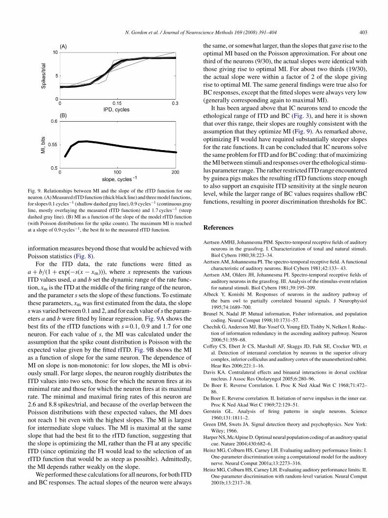

N. Gordon et al. / Journal of Neurosci

Fig. 9. Relationships between MI and the slope of the rITD function for oneneuron. (A) Measured rITD function (thick black line) and three model functions,for slopes 0.1 cycles−1 (shallow dashed gray line), 0.9 cycles−1 (continuous grayline, mostly overlaying the measured rITD function) and 1.7 cycles−1 (steepd(a

iP

a

ItatsebnaeaMoImr2PnfstIrt

a

totttrB(

etaofttlbtlf

R

A

A

A

A

B

C

C

D

D

D

G

G

H

HOne-parameter discrimination using a computational model for the auditory

ashed gray line). (B) MI as a function of the slope of the model rITD functionwith Poisson distributions for the spike counts). The maximum MI is reachedt a slope of 0.9 cycles−1, the best fit to the measured rITD function.

nformation measures beyond those that would be achieved withoisson statistics (Fig. 8).

For the ITD data, the rate functions were fitted as+ b/(1 + exp(−s(x − xm))), where x represents the various

TD values used, a and b set the dynamic range of the rate func-ion, xm is the ITD at the middle of the firing range of the neuron,nd the parameter s sets the slope of these functions. To estimatehese parameters, xm was first estimated from the data, the slopewas varied between 0.1 and 2, and for each value of s the param-ters a and b were fitted by linear regression. Fig. 9A shows theest fits of the rITD functions with s = 0.1, 0.9 and 1.7 for oneeuron. For each value of s, the MI was calculated under thessumption that the spike count distribution is Poisson with thexpected value given by the fitted rITD. Fig. 9B shows the MIs a function of slope for the same neuron. The dependence ofI on slope is non-monotonic: for low slopes, the MI is obvi-

usly small. For large slopes, the neuron roughly distributes theTD values into two sets, those for which the neuron fires at itsinimal rate and those for which the neuron fires at its maximal

ate. The minimal and maximal firing rates of this neuron are.6 and 8.8 spikes/trial, and because of the overlap between theoisson distributions with these expected values, the MI doesot reach 1 bit even with the highest slopes. The MI is largestor intermediate slope values. The MI is maximal at the samelope that had the best fit to the rITD function, suggesting thathe slope is optimizing the MI, rather than the FI at any specificTD (since optimizing the FI would lead to the selection of an
ITD function that would be as steep as possible). Admittedly,he MI depends rather weakly on the slope.
We performed these calculations for all neurons, for both ITDnd BC responses. The actual slopes of the neuron were always

H

ence Methods 169 (2008) 391–404 403

he same, or somewhat larger, than the slopes that gave rise to theptimal MI based on the Poisson approximation. For about onehird of the neurons (9/30), the actual slopes were identical withhose giving rise to optimal MI. For about two thirds (19/30),he actual slope were within a factor of 2 of the slope givingise to optimal MI. The same general findings were true also forC responses, except that the fitted slopes were always very low

generally corresponding again to maximal MI).It has been argued above that IC neurons tend to encode the

thological range of ITD and BC (Fig. 3), and here it is shownhat over this range, their slopes are roughly consistent with thessumption that they optimize MI (Fig. 9). As remarked above,ptimizing FI would have required substantially steeper slopesor the rate functions. It can be concluded that IC neurons solvehe same problem for ITD and for BC coding: that of maximizinghe MI between stimuli and responses over the ethological stimu-us parameter range. The rather restricted ITD range encounteredy guinea pigs makes the resulting rITD functions steep enougho also support an exquisite ITD sensitivity at the single neuronevel, while the larger range of BC values requires shallow rBCunctions, resulting in poorer discrimination thresholds for BC.

eferences

ertsen AMHJ, Johannesma PIM. Spectro-temporal receptive fields of auditoryneurons in the grassfrog. I. Characterization of tonal and natural stimuli.Biol Cybern 1980;38:223–34.

ertsen AM, Johannesma PI. The spectro-temporal receptive field. A functionalcharacteristic of auditory neurons. Biol Cybern 1981;42:133– 43.

ertsen AM, Olders JH, Johannesma PI. Spectro-temporal receptive fields ofauditory neurons in the grassfrog. III. Analysis of the stimulus-event relationfor natural stimuli. Biol Cybern 1981;39:195–209.

lbeck Y, Konishi M. Responses of neurons in the auditory pathway ofthe barn owl to partially correlated binaural signals. J Neurophysiol1995;74:1689–700.

runel N, Nadal JP. Mutual information, Fisher information, and populationcoding. Neural Comput 1998;10:1731–57.

hechik G, Anderson MJ, Bar-Yosef O, Young ED, Tishby N, Nelken I. Reduc-tion of information redundancy in the ascending auditory pathway. Neuron2006;51:359–68.

offey CS, Ebert Jr CS, Marshall AF, Skaggs JD, Falk SE, Crocker WD, etal. Detection of interaural correlation by neurons in the superior olivarycomplex, inferior colliculus and auditory cortex of the unanesthetized rabbit.Hear Res 2006;221:1–16.

avis KA. Contralateral effects and binaural interactions in dorsal cochlearnucleus. J Assoc Res Otolaryngol 2005;6:280–96.

e Boer E. Reverse Correlation. I. Proc K Ned Akad Wet C 1968;71:472–86.

e Boer E. Reverse correlation. II. Initiation of nerve impulses in the inner ear.Proc K Ned Akad Wet C 1969;72:129–51.

erstein GL. Analysis of firing patterns in single neurons. Science1960;131:1811–2.

reen DM, Swets JA. Signal detection theory and psychophysics. New York:Wiley; 1966.

arper NS, McAlpine D. Optimal neural population coding of an auditory spatialcue. Nature 2004;430:682–6.

einz MG, Colburn HS, Carney LH. Evaluating auditory performance limits: I.

nerve. Neural Comput 2001a;13:2273–316.einz MG, Colburn HS, Carney LH. Evaluating auditory performance limits: II.

One-parameter discrimination with random-level variation. Neural Comput2001b;13:2317–38.

4 scien

I

J

J

J

K

K

LL

L

M

N

N

P

P

SS

S

S

S

S

S

S


ngham NJ, Bleeck S, Winter IM. Contralateral inhibitory and excitatory fre-quency response maps in the mammalian cochlear nucleus. Eur J Neurosci2006;24:2515–29.

enison RL. Correlated cortical populations can enhance sound localizationperformance. J Acoust Soc Am 2000;107:414–21.

enison RL, Reale RA. Likelihood approaches to sensory coding in auditorycortex. Network 2003;14:83–102.

oris PX, van de Sande B, Recio-Spinoso A, van der Heijden M. Auditory mid-brain and nerve responses to sinusoidal variations in interaural correlation.J Neurosci 2006;26:279–89.

ang K, Sompolinsky H. Mutual information of population codes and distancemeasures in probability space. Phys Rev Lett 2001;86:4958–61.

eller CH, Takahashi TT. Binaural cross-correlation predicts the responsesof neurons in the owl’s auditory space map under conditions simulatingsumming localization. J Neurosci 1996;16:4300–9.

ehman EL. Theory of point estimation. New York: Wiley & Sons; 1983.ehman EL. Testing statistical hypotheses. 2 ed. New York: Wiley & Sons;

1986.ouage DH, Joris PX, van der Heijden M. Decorrelation sensitivity of auditory

nerve and anteroventral cochlear nucleus fibers to broadband and narrow-band noise. J Neurosci 2006;26:96–108.

iddlebrooks JC, Clock AE, Xu L, Green DM. A panoramic codefor sound location by cortical neurons. Science 1994;264:842–4[see comments].

elken I, Chechik G. Information theory in auditory research. Hear Res2007;229:94–105.

elken I, Chechik G, Mrsic-Flogel TD, King AJ, Schnupp JW. Encoding stim-ulus information by spike numbers and mean response time in primaryauditory cortex. J Comput Neurosci 2005;19:199–221.

Y

ce Methods 169 (2008) 391–404

almer AR, Jiang D, McAlpine D. Desynchronizing responses to correlatednoise: a mechanism for binaural masking level differences at the inferiorcolliculus. J Neurophysiol 1999;81:722–34.

aninski L. Estimation of entropy and mutual information. Neural Comput2003;15:1191–253.

chervish MJ. Theory of statistics. New York: Springer; 1995.hackleton TM, Palmer AR. Contributions of intrinsic neural and stimulus

variance to binaural sensitivity. J Assoc Res Otolaryngol 2006;7:425–42.

hackleton TM, Skottun BC, Arnott RH, Palmer AR. Interaural time differencediscrimination thresholds for single neurons in the inferior colliculus ofGuinea pigs. J Neurosci 2003;23:716–24.

hackleton TM, Arnott RH, Palmer AR. Sensitivity to interaural correlationof single neurons in the inferior colliculus of guinea pigs. J Assoc ResOtolaryngol 2005;6:244–59.

hore SE, Sumner CJ, Bledsoe SC, Lu J. Effects of contralateral sound stimu-lation on unit activity of ventral cochlear nucleus neurons. Exp Brain Res2003;153:427–35.

iebert WM. Some implications of the stochastic behavior of primary auditoryneurons. Kybernetik 1965;2:206–15.

kottun BC, Shackleton TM, Arnott RH, Palmer AR. The ability of inferiorcolliculus neurons to signal differences in interaural delay. Proc Natl AcadSci USA 2001;98:14050–4.

umner CJ, Tucci DL, Shore SE. Responses of ventral cochlear nucleus neu-
rons to contralateral sound after conductive hearing loss. J Neurophysiol2005;94:4234–43.
in TC, Chan JC, Carney LH. Effects of interaural time delays of noise stimulion low-frequency cells in the cat’s inferior colliculus. III. Evidence for cross-correlation. J Neurophysiol 1987;58:562–83.

Responses of neurons in the inferior colliculus to binaural disparities: insights from the use of...

Documents

Transcript of Responses of neurons in the inferior colliculus to binaural disparities: insights from the use of...