Residential construction, land use and the environment. Simulations for the Netherlands using a...

Environmental Modeling and Assessment 6: 133–143, 2001. 2001 Kluwer Academic Publishers. Printed in the Netherlands.

Residential construction, land use and the environment.Simulations for the Netherlands using a GIS-based land use model

Kees Schotten a, Roland Goetgeluk b, Maarten Hilferink c, Piet Rietveld d and Henk Scholten d

a RIVM, Bilthoven, The Netherlandsb Universidade Pedagogica, Beira, Mozambique

c Object Vision, Haarlem, The Netherlandsd Vrije Universiteit, Amsterdam, The Netherlands

E-mail: [email protected]

The present generation of geographical information systems supports strategic planning processes in several ways. They are able tostore, manage and analyse the enormous amount of data needed. Another more output-oriented use is the visualisation of the diversityof locational preferences and perspectives of different interest groups and stakeholders. For the simulation of (more indirect) effects ofautonomous or planned developments land use modelling can be applied. A step further is the definition and implementation of a set ofindicators that show the impact of land use change on different aspects of space and the environment in order to facilitate the (political)discussions, that are an essential part of strategic planning.

This paper focuses on the application of a GIS-based simulation model in the framework of the Fifth National Physical Planning Reportin the Netherlands. The simulation model generates future land use in the Netherlands given several growth scenarios and a spatial strategythat comprises both foreseen strategic and autonomous developments. Special attention is paid to residential construction because this isexpected to be one of the major driving forces in land use changes. An analysis of residential construction for the period 1980–1995 revealsthat residential construction has been relatively concentrated in areas close to existing urban areas. New town policies also played a ratherstrong role during this period. The presence of natural areas (woods and wetlands) plays a significant though limited role in the choicewhere to build new dwellings. The simulation results for the year 2020 are used to assess the effects of land use changes for a range ofenvironmental indicators.

1. Introduction

Spatial planning has returned to the forefront of publicand politic attention. In Europe this is illustrated by therecent adoption of the European Spatial Development Per-spective (ESDP) at the Ministerial conference in Tampere.At the regional and national level numerous examples canbe given such as the release of the (first) Regional Plan forLisbon Metropolitan Area (PROTALM) in Portugal and theFifth National Physical Planning Report in the Netherlands.

Spatial or physical planning can be seen as a strategicspatial policy aimed at finding the optimum adjustment ofspace and society. Often the solutions generated by the par-ties involved, who all have different interests, objectives andpreferences, do not lead to satisfactory results. Therefore,governments are often involved in the planning process thatis described by Healey [1] as a set of governance practicesfor the development and implementation of spatial strate-gies, plans, policies and projects by regulating the location,timing and form of development. These practices are shapedby the dynamics of economic and social change, which giverise to demands of space.

The present generation of geographical information sys-tems (GIS) is used to support these strategic planningprocesses in different ways. Their ability to store, manage,retrieve and visualise the enormous amount of data regard-ing spatial objects needed in the planning process is oftenapplied (e.g., [2]). Also spatial analytical functions to assess

relevant spatial patterns are widely used. Another develop-ment is the linkage of GIS with location or allocation mod-els and more recently the integration of accessible computerbased applications or Decision Support Systems.

Various model approaches can be distinguished in thefield of land use (cf. [3]):

1. Planning models. These models compute an optimal al-location of land in order to arrive at a maximum valuefor some optimisation criterion (for example, maximumprofit of a farm), or to maximise some social welfare ob-jective strived after by a public sector planner (see, e.g.,[4]).

2. Individual choice models. These models describe the lo-cational preferences of individual actors on the basis ofindividual decision process [5].

3. Al-models derived from the field of Artificial Intelligence.Examples of these allocation algorithms are Neural Net-works (NN), Genetic Algorithms and Cellular Automata(CA). Applications of Al-models in the field of allocationplanning are, e.g., described in [6–9].

4. Equilibrium models explaining land use in terms of sup-ply, demand and equilibrium prices. These models arepart of the tradition of the classical approaches of VonThunen, Losch and Alonso. In most of these modelstransport and accessibility play an important role as de-terminants of the equilibrium outcomes of land use. Ex-

134 K. Schotten et al. / Residential construction, land use and the environment

amples of operational models used in planning contextsare those of Anas [10] and Landis [11].

In this paper we will use make use of a model of the lattercategory.

An interesting development is that these land use modelsare linked to environmental models in order to be able toassess the environmental consequences of land use change(for a review see [12]. For example, changes in land use willhave consequences for spatial interaction patterns and these,in turn, will have an impact on emission and noise caused bytransport (see also [13]).

This paper focuses on the application of a GIS-based landuse model to the Fifth National Physical Planning Reportin the Netherlands. The model generates future land use inthe Netherlands given several growth scenarios and a spa-tial strategy that comprises both foreseen strategic and au-tonomous developments. The simulation results, a map withresidential areas and an integrated land use map, are used toassess the effects of land use changes on a wide range of en-vironmental indicators. We focus on land use for residentialpurposes because this is a very dynamic land use category inthe Netherlands. In terms of modelling, most attention willbe paid to the Land Use Scanner, a GIS-based model for theNetherlands. Models assessing land use implications for theenvironment will only be discussed briefly.

The structure of the paper is as follows. We start witha short review of the backgrounds of physical planning inthe Netherlands and of possible changes in external condi-tions (section 2). The land use scanner model is presented inmore detail in section 3. Changes in land use for residentialpurposes during the period 1980–1995 are analysed in sec-tion 4. This is followed by a simulation of future patterns inresidential construction in section 5. Environmental impactsare analysed in section 6.

2. Background of the study

The Netherlands is among the most densely populatedcountries in the world. Given the high externalities that oc-cur in land use, it is no surprise that the government is quiteactive in interfering with the land market. Especially in de-cisions on the location of residential areas the governmentplays a strong role. The long run national policies on landuse are formulated in strategic policy memoranda, the lastof which appeared in 1988. The next document called theFifth National Physical Planning Report will be published in2000. In the preparatory phase the National Institute of Pub-lic Health and Environment (RIVM) analysed basic uncer-tainties for the future by means of scenarios. Possible conse-quences for land use and the environment during the period1995–2020 (the Fifth Report’s time span) were investigated.

Aim of the study is not to deliver a blueprint for landuse in 2020, nor to simply quantify the impacts of land usechange on the environment, but to establish a objectifiedmethodology making use of models to enable discussionson future land use developments. Of course, the discussions

can embrace the necessary operational assumptions made inorder to obtain results and can also be used to gain under-standing of land use dynamics and (indirect) effects on theenvironment. The main goal, however, is to enable the eval-uation of spatial policies and to assess the environmental ef-fects of alternative spatial policies.

2.1. Scenarios

An important element that shapes spatial planning prac-tices is the expected rise or decline in demand for space thatresults from the dynamics in economic and social change.In order to cope with the uncertainties of future demandsfor space the concept of scenarios is often used [14]. Inthis study three internally consistent and coherent scenarios,developed by The Dutch Central Planning Bureau [15], areused to describe demographic, economic, social and policydevelopments until 2020. These scenarios can be charac-terised as follows.

– Divided Europe (DE): protectionistic tendencies in thedifferent European countries are strong. Economicgrowth is low with an annual rise in BNP of approx.1.7%. The population grows to 16.3 million while thenumber of dwellings rises to 7.5 million (currently 15and 6.2 million, respectively). The Common AgriculturalPolicy (CAP) is continued.

– European Co-ordination (EC): The world economy isdominated by trade organisations resulting in an accel-erated integration of the European countries. The annualeconomic growth is moderate (3.0%) but the growth inpopulation to a total of 17.7 million is the highest of allscenarios. The number of dwellings grows to 7.8 mil-lion. A unified European policy is implemented implyinga certain level of protection of agriculture in the commonmarket.

– Global Competition (GC): Market forces dominate theworld economy and the economic growth is high (3.3%).The number of inhabitants rises to 16.9 million. How-ever, due to a more individualistic life style the numberof dwellings grows to 8.1 million, faster than in the ECscenario. The CAP is abandoned forcing the agriculturalsector to compete on the world market.

Taking the developments described in the CPB scenarios asa starting point different sector-specific models are used tocalculate the amount of land needed for agriculture, housing,industrial and commercial areas in each of the scenarios. Theresults are shown in figure 1.

The demands for nature and (rail and motorway) in-frastructure in the Netherlands are determined by policiesthat have already been agreed, so that the claims of theseland use types are identical in each of the scenarios. Na-ture (including forest) is also the land use type that claimsthe largest amount of land until 2020 in each of the scenar-ios. While the claims for housing, industry and commerceare less than that for nature, they also vary due to the dif-ference in foreseen dwellings and economic growth within

K. Schotten et al. / Residential construction, land use and the environment 135

Figure 1. Sectoral land use demands in the three scenarios.

the scenarios. In all scenarios the area used for agriculturedeclines, only the rate differs in each scenario; high in theDivided Europe and Global Competition scenarios and lowin European Coordination. For the Netherlands this resultsin a surplus of land in the GC scenario and a more or lessbalanced situation in the DE-scenario. In the EC scenarioa situation is reached where the demand for land exceedsthe supply by 46000 ha. This calls for a reconsideration ofthe claims computed by the sectoral models. An integratedanalysis of demand for land across various land use types isnecessary to arrive at such a conclusion. Such an integratedanalysis will be the subject of the next section. The model tobe used for this purpose is the LAND USE SCANNER andit will be discussed in the next section.

3. The LAND USE SCANNER model

3.1. General features

We start with a short characterisation of the properties ofthe LAND USE SCANNER. Some characteristic features ofthe model are:

• Grid based. The model describes for all grids in a systemthe relative proportions of land to be used for a numberof land use types. Model specification and software al-low large numbers of grids. The present version covers193,399 grid cells of 500 by 500 meters each, coveringall of the Netherlands.

• Integrated. The model provides an integration frameworkfor sectoral data bases and sectoral policy proposals byconfronting these inputs in a spatial-analytical context.

• Exhaustive. The model is exhaustive in the sense that allgrids in a spatial unit (in our case a country) are consid-ered. All types of land use are explicitly considered; thusthere are no “rest” categories left untreated. The modelcan be formulated in such a way that transfers of wetgrids (sea, lakes) into land are allowed.

• Dynamic. The model deals with changes in land use tak-ing into account present land use patterns. The suitabil-ities of the grids for certain types of land use are not as-

sumed constant, but may change as the result of changesin land use in the course of time.

• Satellite structure. The model is driven by forecasts ata national or regional level in terms of variables such aspopulation, agricultural production, infrastructure, etc.

• Stochastic. The outcomes of the model are to be inter-preted as expected proportions of land to be used for var-ious types of land use categories. The use of the model isnot that it predicts land use in particular small grids in thefuture. The main use of the model is that it gives the im-plications for the spatial patterns of land use of processessuch as population growth, production (manufacturing,agriculture, etc.), and natural conservation.

• Policy oriented. Several types of sectoral policies havestrong spatial implications. LAND USE SCANNERmakes these implications explicit. The model helps solv-ing questions referring to the types of grids in which ma-jor policy conflicts can be expected to emerge. It canalso be used to investigate the implications of sectoraland macro policies for human settlement and land usepatterns.

The property of integration means that the LAND USESCANNER can function as a tool to improve communica-tion between analysts working in various fields of land use(for example, urban functions versus agriculture versus nat-ural land use). The model also helps to improve consistencybetween projections made in these fields. Thus a potentialuse of the LAND USE SCANNER is that is does not onlyfunction as a modelling tool, but also as a communicationtool between analysts in various policy fields.

The following types of land use are distinguished in thepresent version of the model:

1. Urban: residential, industrial, roads, railways, and air-ports.

2. Agriculture: pasture, corn, arable land (potatoes, beets,cereals), flower bulbs, orchards, cultivation under glass,and other agriculture.

3. Natural areas: wood, nature.

4. Water.


We arrive at 15 different land use types. This number ofland use types can be extended. Data are available for morefinely meshed distinctions, thus leading to up to 40 land usecategories.

3.2. Regional constraints, suitability maps and governmentinterventions

The LAND USE SCANNER model is driven by out-comes of other sector specific models which generate re-sults at a much lower spatial detail. The outcomes relateto the year 2020. The projections for agricultural land useand urban functions have been made for the various scenar-ios mentioned in the preceding section. Thus, a check has tobe conducted to ensure consistency of inputs (see below).

Projections of demand for land at the regional level areavailable among others for various types of agriculture areavailable for agricultural regions, of which there are 14 inthe Netherlands. For residential and industrial areas pro-jections are given at the level of so-called COROP regions.There are 40 COROP regions in the Netherlands. For naturalareas regional constraints are included for 66 regions. Theconstraints imply that the total amount of land used by na-ture must be at least the amount which is set as a minimumamount for each region in government plans.

The demand side of the land market is represented bysuitability maps. A suitability map is generated for each landuse type to indicate the suitability of each grid cell for thattype. These suitability maps can be interpreted as bid-prices.The suitabilities depend on factors such as:

• soil quality,

• transition costs, given previous land use,

• accessibility of facilities and infrastructure,

• amount of similar land use in the neighbourhood.

In Hilferink and Rietveld [16] more details are given aboutthe computation of suitability maps.

In addition to suitabilities expressing bid prices of marketactors, governmental planning regulations have an impact onland use developments. These include:

• policies towards building permits for residential and in-dustrial land use,

• policies regarding the preservation and development ofnatural areas.

These policy interventions can be interpreted as subsidiesand taxes for certain types of land use so that the final marketoutcome does not merely reflect the willingness to pay ofactors at the market. Also the intentions of the public sectorto stimulate or discourage land use of particular types are tosome extent reflected by the resulting land use patterns.

3.3. Mathematical formulation

A core variable of the model is the suitability scj for landuse of type j in grid cell c. This suitability represents the net

benefits (benefits minus costs) of land use type j in cell c.The higher the suitability for land use type j , the higher theprobability xcj that the cell will be used for this type. In thesimplest version of our model we use a logit type approachto determine this probability:

xcj = exp(β · scj )∑j exp(β · scj )

for all c and j . (1)

Thus, when β is zero, all types of land use have the sameprobability; i.e., the suitability factors scj do not play anyrole in determining these shares. On the other hand, whenβ goes to infinite, the limit of probability that the categorywith the highest suitability gets the cell is equal to 1.

In terms of expected values, the expected volume of landuse Lcj for category j in cell c equals:

Lcj = xcj · Lc for all c and j, (2)

where Lc denotes the total volume of land in cell c. Withequally sized cells Lc would of course be equal for all c. Un-equally sized cells may occur in the case of cells located nearthe national border, or cells being partly water (if a transferfrom water to non-water land use is not allowed), or containpreset land use based on exogenous data, such as infrastruc-ture developments.

The model as formulated here does not guarantee that theallocation of space across possible land uses is in accordancewith overall demand conditions. Therefore, side constraintshave to be imposed in order to ensure that at the relevantlevels of aggregation total demand is met.

This leads to a reformulation of the model. Let Dj bea restriction on total demand for land use category j . Inaddition, let Mcj denote the expected amount of land in cellc that will be used for category j taking into account the sideconstraints. We then arrive at a doubly constrained model:

Mcj = aj · bc · exp β · scj for the constrained j and all c,

(3)where aj and bc are balancing factors such that the followingconstraints are satisfied:∑

c

Mcj = Dj for the constrained j, (4)

∑j

Mcj = Lc for all c. (5)

Equation (4) guarantees that the expected amount of land al-located for land use type j equals the imposed amount Dj .In addition, equation (5) implies that the sum of the expectedvolumes of the various land use types per cell is equal tothe total area of each cell. We use the expression “for theconstrained j” when an aggregate constraint has been for-mulated for the particular land use type j . It is clear thatthe constraints may imply that no feasible solution exists.This can be checked by seeking for a starting solution of thesystem in a linear programming context. When no feasiblesolution is found, the aggregate constraints have to be re-considered before the model can be used. For those land use


types j for which no aggregate constraint applies we arriveat:

Mcj = bc · exp β · scj for unconstrained j and all c (3′)

under constraint (5) so that we may conclude that in this caseaj has been set equal to 1. Note that in the extreme case thatnone of the land use types has any aggregate constraints, wehave Mcj = Lcj for all c and j , and bc = Lc/

∑j exp(β ·scj )

for all c.

3.4. Balancing factors

The above reformulation as a doubly constrained land usemodel is helpful for an understanding of the structure of themodel. The structure of the model is quite similar to doublyconstrained spatial interaction models used in transportationresearch (see, for example, [17]). We now turn to the inter-pretation of the balancing factors. From equations (3)–(5) itfollows that:

bc = Lc∑j aj · exp(β · scj )

for all c, (6a)

aj = Dj∑c bc · exp(β · scj ) for the constrained j, (6b)

aj = 1 for the other j . (6c)∑c bc · exp(β · scj ) can be interpreted as the aggregate suit-

ability of land for land use type j ; when the suitability ofland use type j would be low in terms of scj , the value of thedenominator in (6b) is low as well. The balancing factor aj

is high when a high constraint Dj is combined with a lowaggregate suitability.

In a similar way∑

j aj · exp(β · scj ) in (6a) can be inter-preted as a measure of demand for land use in cell c. A highvalue of this expression means that the demand for the landin cell c for the various land use types (taking into accountthe urgency of the land use types as represented by aj ) isrelatively high. It leads to a low value of the balancing fac-tor bc, and thus ensures that in equation (5) the total amountof land finally allocated in cell c does not exceed the supplyof available land Lc. Thus, the solution of the doubly con-strained model yields as a side-product the shadow pricesof land in the cells. Another way to interpret the balancingfactors is to rewrite equation (3) as:

Mcj = exp(β · [

scj + β−1 · log(aj ) + β−1 · log(bc)])

for the constrained j and all c. (3′′)

A large value of aj implies a strong pressure on land usetype j . It can be interpreted as a subsidy to this type of landuse; the subsidy is given to ensure that the aggregate targetfor land use type j is achieved. The reverse case is a smallvalue for aj ; this can be interpreted as a tax on this landuse type to prevent that excess of the related target. Notethat the case in between occurs when aj equals 1, implyinglog(aj ) = 0.

In order to clarify the role of the balancing factors, weperform the following transformation on (3′′). Define land

use price pc in cell c as −(1/β) · log(bc) and price λj forconstraint j as +(1/β) · log(aj ), now Mcj can be consideredas a demand function of land use price pc

Mcj (pc) = exp(β · scj + λj − pc). (3′′′)

This formulation also sheds light on the bc factor. A highvalue of bc means that use of cell c is discouraged. It cantherefore be interpreted as an indicator of demand/supplyconditions in each cell.

An increase in the aggregate demand of category j willlead to a shift in land use in the following way. The highervalue of Dj will lead to a higher balancing factor aj , whichwill lead to a corresponding increase in the expected landuse in the various grids depending on the relative suitabilityof the grids for the various types of land use.

3.5. Extensions to the doubly constrained land use model

In reality the model is more complex than presented here.One complication is that the constraints are not always interms of equalities, but in terms of inequalities. Consider theconstraint that: ∑

c

Mcj � Dj . (4′)

Then in the case when the constraint is not binding, we haveaj = 1, and when the constraint is binding we have aj asdefined in (6b). Thus, in this case we arrive at:

aj = max

{1,

Dj∑c bc · exp(β · scj )

}

for all lower bounded j . (7)

In the case of an � constraint we arrive at:

aj = min

{1,

Dj∑c bc · exp(β · scj )

}

for all upper bounded j. (8)

Another complication is that the aggregate constraints notonly function at the level of the country, but also at variousregional levels. This means, for example, that populationpredictions have been made for labour market regions, orthat agricultural production has been predicted at the levelof agricultural areas. This leads to an extended version ofthe model where the balancing factor aj becomes specificfor each region for which a constraint has been formulated.

Solution of the model is done in an iterative way. In thecase of equality constraints, it only boils down to finding thevalues of aj and bc in equations (6a)–(6c).

Beginning with arbitrary values for the aj , one can com-pute the resulting values for bc by means of (6a). Then thesebc values are fed into equation (6b) leading to revised valuesfor aj .

In the case where some of the constraints are in termsof inequalities, one should use equations (7) and (8) insteadof (6b). Once these factors have been determined, the im-plied land use pattern can easily be found by means of equa-tion (3).


3.6. Interpretation in terms of market equilibria

In section 1 we indicated that the land use scanner modelbelongs to the class of equilibrium models. Equilibriumtakes place at the macro-level: aggregate supply for land isgiven (it is assumed to be inelastic) and aggregate demandfor land for various land use types is also given at the level ofregions. Inequality constraints (see equation (4′)) ensure thataggregate demand does not exceed aggregate supply. Pricesdo not play a role at the aggregate level in the present ver-sion of the model since both demand and supply are priceinelastic at this level. Future development of the model maylead to the specification of elastic demand functions at theaggregate level.

Also at the level of individual cells demand and supplyof land are in equilibrium (see equation (5)). Balancing fac-tors are used to achieve this. These balancing factors can beinterpreted in terms of shadow prices (see (3′′′)). Cells withhigh suitability for various types of land use will have a highshadow price to ensure that demand does not exceed supply.Note, for example, that in (3′′′) the shadow price pc func-tions as a correction factor for a high level of suitability scj .

4. An analysis of changes in residential land use1980–1995

In this section we discuss the estimation of suitability in-dicators for housing. This will be done for the period 1980–1995. In the next section the outcomes of this estimation willbe used for a simulation during the period 1995–2020. Resi-dential construction in the Netherlands is subject to two mainforces: the preferences of the residents and the directionsof the national and regional governments. Especially in theWestern part of the country the government plays an impor-tant role by commanding residential construction at certainnew town and by discouraging urban sprawl. It is impossibleto separate the two driving forces. This means that the es-timations of determinants of residential construction reflecta mixture of private sector preferences and public sector ob-jectives.

The data on which the estimations are based relate to thegrowth of the housing stock in grids. We consider the spaceavailable for residential construction in 1980 in each grid cellas a starting point. Since we consider only open space thepossibilities for residential construction within urban areasare low. The dependent variable in the analysis is the shareof available land in each that is ultimately used for residen-tial construction. For details on the estimation procedure werefer to Wagtendonk and Rietveld [18]. The following typesof factors are assumed to play a role in the attractiveness ofresidential location:

• accessibility of work locations,

• proximity of other residential areas,

• accessibility of natural areas,

• distance to highway access points and to railway stations,

• presence of highways and railway lines in a grid.

The accessibility of work locations is taken into account bycomputing for each grid cell the weighed sum of the num-ber of jobs in the grids until a distance of 60 km. For theweights distance decay factors are used that have been cal-ibrated for commuting trips. Accessibility indicators havebeen computed for various types of jobs. It appears that theseare highly correlated, implying a multi-collinearity problem.Therefore it does not make sense to include accessibility forseveral types of jobs in the same regression.

Proximity to other residential areas is used to reflect pref-erences of residents to live in places where there is sufficientsupply of urban facilities and the public sector objective toprevent urban sprawl. The latter means that residential con-struction is stimulated to take place in a spatially concen-trated form: in open spaces within urban areas and near ex-isting residential areas. This variable is measured by com-puting for each grid cell the total area used for residentialpurposes in the 8 contiguous grids. A related indicator is theintroduction of a dummy for new towns in those grids wherethe national government has planned the location of a newtown.

Accessibility of natural areas is included to take into ac-count the natural values in the surroundings of grids. Foreach grid cell the surfaces of forest areas and wetlands withina circle of 15 km are computed. These surfaces are weightedby means of distance decay factors in a similar way as withthe accessibility of jobs.

As a negative indicator of the quality of the natural en-vironment in a grid cell we introduce the presence of in-frastructure (highways and railway lines). We expect thatthe noise problems involved will discourage developers tobuild residences in such a grid. Of course, infrastructurealso yields accessibility, but this is not necessarily correlatedwith the presence of these infrastructures in a grid, becausethey depend more in particular on the location of highwayaccess points and railway stations. This is reflected by thenext indicator.

Distance to highway access points and to railway sta-tions. These variables are measured via the distance to thenearest highway access point and the nearest railway station.They are general indicators of the appreciation of consumersto live at locations that offer them easy access to high qualitytransport networks.

The analysis has been carried out for two types of dwell-ings (one dwelling houses and multiple dwelling houses).The multiple dwelling houses are mainly found in urban ar-eas. Another distinction used is the one between the mosturbanised area (Randstad Holland) and the rest of the coun-try. The reason is that in the former part the degree of gov-ernment intervention is much higher. Thus we arrive at fourdifferent segments for which estimations have been carriedout. The results are summarised in table 1.

We find that in Randstad accessibility of jobs did not playa role for one dwelling houses. A possible explanation isthat within this highly urbanised area accessibility of jobs


Table 1Parameters of the four regression equations that explain the location of new residential areas over the period 1980–1993.

One dwelling house Multiple dwelling houseRandstad Holand Other regions Randstad Holand Other regionsB T -value B T -value B T -value B T -value

Intercept –7.02 –389.6 –20.35 –255.6 –11.81 –462.2 –15.02 –329.8Industry not applicable not applicable 0.28 121.4 not applicableKnowledge services not applicable 1.00 160.0 not applicable 0.34 79.3Forest for leisure purposes –0.02 –27.5 0.06 36.0 0.04 39.9 not applicableWetlands not applicable not applicable 0.07 69.1 0.11 39.6Highways –0.34 –94.7 –0.36 –69.6 –0.11 –42.5 –0.15 –27.0Railways –0.58 –91.3 0.05 7.0 –0.37 –85.1 –0.30 –35.8Highway accesses 0.04 33.0 0.12 61.3 –0.12 –117.2 not applicableRailway stations –0.14 –103.5 –0.12 –87.4 0.05 56.6 –0.18 –109.7Growth centers 1.13 264.0 0.74 101.0 1.63 366.0 1.08 121.6One-family dwellings 0.73 548.0 0.54 242.1 0.83 934.1 0.88 300.8Multiple-family dwellings 0.06 75.7 0.39 331.7 0.10 126.0 0.50 328.7

Pseudo R2 0.67 0.59 0.41 0.50

is high anywhere so that a negligible impact results. Forthe other three market segments considered the accessibil-ity of jobs did play a role in residential construction dur-ing the period considered. Accessibility of wetlands andforest areas appears to play a role in all market segments:with one exception we find that residential construction isstimulated by the presence of natural areas in the region.Also the other environmental indicators (presence of high-ways and railways) have the expected signs. In grid cellswhere these infrastructures are present the probability thatopen land will be converted into residential use is smallerthan in other regions. Distances to railway stations tend tohave a negative impact on the probability of residential con-struction in a zone. This can partly be explained by gov-ernmental policies to stimulate residential construction nearrailway stations. As indicated by Rietveld [19] such a pol-icy of building near railway stations certainly makes sensegiven the importance of non-motorised transport modes asaccess modes to the railway network. For highways distancedoes not play such a clear role as a determinant of residentialconstruction.

Spatial patterns of existing dwellings have a very strongimpact on residential construction. Table 1 shows for allmarket segments that new residences tend to be built in theimmediate neighbourhood of existing residential areas. Inaddition to existing residential areas new towns appear toplay an important role in residential construction between1980 and 1995. For all market segments the assignment ofa new town (or growth centre) status has led to a strongincrease in residential construction in the grid cells con-cerned.

5. Simulation of future land use

Based on estimates of suitabilities for various types ofland use and on national and regional totals for certain typesof land we have simulated the developments of future land

use. We start with a discussion of land for residential pur-poses.

5.1. Residential land use

The pattern illustrated by figure 2 underlines the strongposition of the current large cities in the Netherlands (Am-sterdam, Rotterdam, The Hague and Utrecht) in the Centraland Western part of the country. Given the concentrationof work locations in these areas it is here where the high-est probabilities can be found that open space is used forthe construction of new housing. In addition, there is a con-siderable number of medium sized cities that appear to beattractive locations for residential activities. A differencebetween single and multiple family dwellings is that the lat-ter are expected to be much more concentrated in the urbanareas. This makes sense given the higher land prices, thesmaller household size and the lower income levels usuallyobserved in urban areas in the Netherlands.

Part of figure 2 is based on government plans in physicalplanning that have been formulated in earlier stages and thathave not yet been implemented, but where the realisation is(almost) sure. Another part of figure 2 is based on the modelparameters estimated in table 1. This means that we assumethat the parameters estimated for the period between 1980and 1995 also hold for the period after it. For example, weassume that the role of the attraction of proximity to work lo-cations in residential construction remains unchanged duringthe periods considered. Other assumptions could of coursehave been formulated. For example, one might conjecturethat proximity to work locations becomes less important inview of the potential of ICT induced telecommuting. Wehave abstained from such a broad analysis of possible fu-tures. Thus the results presented here are based on the as-sumption that preferences of physical planners, real estatedevelopers and public sector remain unchanged. The only


Figure 2. Regression based probabilities of the allocation of one and more-family dwellings for the period 1995–2020.

Figure 3. Location of the new residential areas simulated for the period 1995–2010 and 1995–2020 according to the EC scenario.

uncertainties considered in the present paper relate to the el-ements of the scenarios (see section 3).

On the basis of figure 2 one can derive predictions of theextent to which zones will experience a change into land usefor residential purposes. The results are presented in figure 3for the CE scenario. This means that population is assumedto increase from 15.5 million in 1995 to 17.7 million in 2020.All provinces except for the province of Zealand (located inthe South West) are expected to experience major expansionof residential areas. Most expansion is expected to take placein the vicinity of the present cities plus in a very limitednumber of new towns. For the other scenarios maps withsimilar patterns result. The scenarios do not so much differin terms of spatial development patterns but more in terms of

speed of expansion of the area used for residential purposes.A striking difference between figures 2 and 3 is that in

figure 2 the existing major urban areas can easily be iden-tified, whereas they remain invisible in figure 3. The rea-son is that figure 2 demonstrates the probability that landcan be used for residential construction assuming that it isopen land. Since most of the land in the urban areas is al-ready used for urban activities it plays only a small role inthe reallocation of land for residential use as shown in fig-ure 3. Figure 3 shows that open areas rather close to theexisting cities are expected to dominate residential construc-tion.1

1 Thus, figure 3 is most relevant when one is interested in absolute changesin land use, whereas figure 2 represents relative changes in landuse.


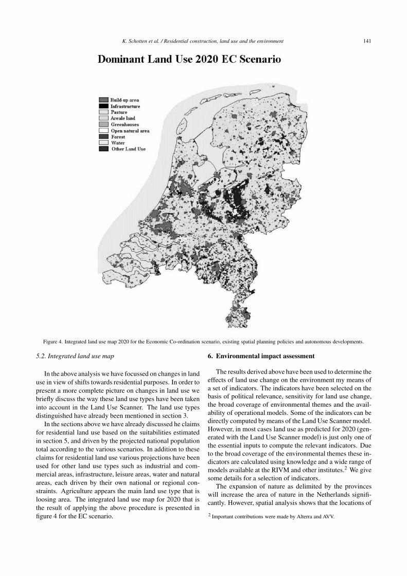
Figure 4. Integrated land use map 2020 for the Economic Co-ordination scenario, existing spatial planning policies and autonomous developments.

5.2. Integrated land use map

In the above analysis we have focussed on changes in landuse in view of shifts towards residential purposes. In order topresent a more complete picture on changes in land use webriefly discuss the way these land use types have been takeninto account in the Land Use Scanner. The land use typesdistinguished have already been mentioned in section 3.

In the sections above we have already discussed he claimsfor residential land use based on the suitabilities estimatedin section 5, and driven by the projected national populationtotal according to the various scenarios. In addition to theseclaims for residential land use various projections have beenused for other land use types such as industrial and com-mercial areas, infrastructure, leisure areas, water and naturalareas, each driven by their own national or regional con-straints. Agriculture appears the main land use type that isloosing area. The integrated land use map for 2020 that isthe result of applying the above procedure is presented infigure 4 for the EC scenario.

6. Environmental impact assessment

The results derived above have been used to determine theeffects of land use change on the environment my means ofa set of indicators. The indicators have been selected on thebasis of political relevance, sensitivity for land use change,the broad coverage of environmental themes and the avail-ability of operational models. Some of the indicators can bedirectly computed by means of the Land Use Scanner model.However, in most cases land use as predicted for 2020 (gen-erated with the Land Use Scanner model) is just only one ofthe essential inputs to compute the relevant indicators. Dueto the broad coverage of the environmental themes these in-dicators are calculated using knowledge and a wide range ofmodels available at the RIVM and other institutes.2 We givesome details for a selection of indicators.

The expansion of nature as delimited by the provinceswill increase the area of nature in the Netherlands signifi-cantly. However, spatial analysis shows that the locations of

2 Important contributions were made by Alterra and AVV.


new natural areas are so scattered that the cohesion of nat-ural areas develops in a less favourable way than the increasein natural area. The quality of the flora in the Netherlandsis calculated with the Nature planner model. The value ofthe indicator is a product of nature quantity and the naturequality expressed as the occurrence of selected plant species[20]. The increase in nature quality can be preliminary con-tributed to the restoration of the ground water levels. Reduc-tion in acidification and fertilisation are too small to have asignificant influence.

Spatial analyses regarding safety show that new built upareas are located in areas in danger of flooding and water ex-cess, taking into account the water drainage in 2020. Whileother land use types like natural areas are also not plannedat locations were they can have a reducing effect on floodingand water excess.

The model FACTS [21] is used to calculate the owner-ship, fuel cost and energy use of passenger cars in 2020. Carownership and fuel cost are, in conjunction with the LandUse Scanner results, used to calculate the use of cars on anaverage working day making use of the LMS-Model [22].The outputs of the LMS model are on their part again usedto calculate the noise nuisance (making use of the model de-scribed in [23] and the accessibility of jobs by the labourforce with a commuting time lower than 45 minutes [24].

The overall conclusion of the comparison between thepresent situation and the simulation for 2020 is that the envi-ronmental quality is improving, although one has to keepin mind that currently implemented policies without spa-tial aspects also have positive impacts on the environmentalquality in the year 2020. Especially the indicators dealingwith nature are positive owing to the realisation of more than150,000 hectares of new nature. This is about 4% of the totalarea of the country and implies a considerable shift in landuse. The background of this increase is that agricultural ar-eas are replaced by natural areas. Not only the total size ofnatural areas is improving, also the cohesion of natural areasis getting better. Cohesion is measured in terms of the degreeto which the cutting up of natural areas has been avoided. Itis an important qualitative aspect of nature since in additionto total area also the existence of barriers between naturalareas has an impact on ecosystems.

The environmental indicators show that an increase inCO2 emissions is expected. The improvement of energy ef-ficiency of cars is more than off-set by an increase in caruse and an increase in the weight of cars. The amount ofnitrate that leaches to groundwater, and threatens its use fordrinking water, decreases.

The new housing developments have a negative impact onthe landscape indicators. Even though new residential areastend to be built near to existing residential areas there is atendency that the openness of landscapes (measured via theextent to which built areas interfere with open space) deteri-orates. Another aspect of the expected residential construc-tion activities is that in vulnerable regions in the Netherlandsthe flooding hazard and the chance on water excess increasesmoderately.

7. Concluding remarks

The analytical possibilities of geographical informationsystems have been improved substantially by linking themto land use models. This enables planners to assess the pro’sand con’s of various spatial principles or to value the effectsof spatial strategies on policy targets or societal aims. More-over, it opens the way to a much more quantitative approachto planning that can complement the present more qualita-tive planning practice.

This study shows that it is possible to anticipate complexland use dynamics and their environmental impacts. Due tothe developments in the IT world in general and the world ofGeographic Information Systems in particular the problemsencountered are no longer technological. When the centralobjective is to support decision makers the main concerns areto ensure that the numerous different models involved makeuse of the same validated data and that the quality and limita-tions of intermediate results are known to those researchersthat use them for further processing.

The simulated land use dynamics, which form the finalresult of a complex allocation methodology, give an ex-planatory overview of the locational preferences of the se-lected land use types and their mutual interactions. It is rec-ommended that auxiliary information regarding demand forland, suitability maps, etc. is also made available to the de-cision maker(s) involved in strategic planning. This does notonly help to gain insight in the driving forces that affect landuse but may also support the formulation of alternative spa-tial strategies.

An interesting conclusion from section 6 is that duringthe period from 1995 to 2020 there is substantial scope forimprovement for the size of natural areas in the Nether-lands, even though the population is expected to increasewith about 15% and total area claimed for urban activitiesincreases substantially. The reason is that there is still suffi-cient area from agriculture that can be converted into naturalareas or into urban area. The results for the quality of thelocal environment are mixed. On the one hand pollution ofground water and ammonia deposition are expected to im-prove. However, according to indicators related to quietingof landscape, openness of landscape and historical values oflandscape will deteriorate. Therefore a challenging themefor future research and policy is to broaden the issue of con-servation or expansion of natural areas to the more generaltheme of the improvement of qualities of landscapes.

Acknowledgements

The authors thank the following colleagues: WidekeBoersma (Geodan) and Camiel Heunks (RIVM) for theirhelp running the Land Use Scanner Model; John Helming(LEI) for the calculations of the agricultural demands withthe DRAM model; Alfred Wagtendonk (VU) for his workon the housing demand equation, and Karst Geurts as wellas Rob Alkemade (RIVM) for their work on the impact as-sessments.


References

[1] P. Healey, The revival of strategic spatial planning in Europe, in: Mak-ing Strategic Spatial Plans: Innovations in Europe, eds. P. Healey,A.M. Khakee and B. Needham (UCL Press, London, 1997) pp. 3–19.

[2] RPD, Nederland in Plannen 1999: ruimtelijke functieveranderingentot ca. 2010. Appendix of: Balans Ruimtelijke kwaliteit 1999: Beeldop hoofdlijnen, Ministerie van VROM, The Hague (1999) 40 p.

[3] M. Grothe, Keuze voor ruimte, ruimte voor keuzen. De ontwikkel-ing van GIS applicaties voorpocatieplanning; een objectgeorienteerdeanalyse, Phd dissertation, Vrije Universiteit, Amsterdam (1998).

[4] R.A. Schipper, Farming in a Fragile Future (Wageningen AgriculturalUniversity, Wageningen, 1996).

[5] H.J.P. Timmermans, Decision models for predicting preferencesamong multiattribute choice alternatives, in: Recent Developmentsin Spatial Data Analyses: Methodology, Measurement and Models,eds. G. Bahrenberg, M.M. Fisher and P. Nijkamp (Gower, Aldershot,1984) pp. 337–355.

[6] K.A. Raju, P.K. Sikdar and S.L. Dhingra, Micro-simulation of resi-dential location choice and its variation, Computers, Environment andUrban Systems 22(3) (1998) 203–218.

[7] A.G. Pereira, G. Munda and M. Paruccini, Generating alternatives forsiting retail and service facilities using genetic algorithms and mul-tiple criteria decision techniques, Journal of Retailing and ConsumerServices 1 (1994) 40–47.

[8] F. Wu, A linguistic cellular automata simulation approach for sustain-able land development in a fast growing region, Computers, Environ-ment and Urban Systems 20(6) (1996) 367–387.

[9] R. White, G. Engelen and I. Uljee, The use of constrained cellularautomata for high-resolution modelling of urban dynamics, Environ-ment and Planning B 24 (1997) 323–343.

[10] A. Anas, Residential Location Models and Urban Transportation(Academic Press, New York, 1982).

[11] J. Landis, The California urban futures model: a new generationof metropolitan simulation models, Environment and Planning B 21(1994) 399–420.

[12] Y. Hayashi and J. Roy, Transport, Land Use and the Environment(Kluwer, Dordrecht, 1996).

[13] W. Young and D. Bowyer, Modelling the environmental impact ofchanges in urban structure, Computers, Environment and Urban Sys-tems 20(4/5) (1996) 313–326.

[14] F.Th. Schoute, P.A. Finke, F.R. Veeneklaas and H.P. Wolfert, eds.,Scenario studies for the rural environment, in: Proceedings of theSymposium Scenario Studies for the Rural Environment, Wageningen(Kluwer Academic Publishers, Dordrecht, 1997).

[15] Central Planning Bureau, Economie en Fysieke Omgeving (Sdu Pub-lishers, The Hague, 1997).

[16] M. Hilferink and P. Rietveld, Land use scanner: an integrated modelfor long term projections of land use in urban and rural areas, Journalof Geographical Information Systems 1 (1999) 155–177.

[17] A.S. Fotheringham and M.E. O’Kelly, Spatial Interaction Models:Formulations and Applications (Kluwer, Dordrecht, 1989).

[18] A.J. Wagtendonk and P. Rietveld, Ruimtelijke ontwikkelingenwoningbouw Nederland, 1980–1995: Een historisch-kwantitatieveanalyse van de ruimtelijke ontwikkelingen in de woningbouw in deperiode 1980–1995, ter ondersteuning van de Omgevingseffectrap-portage Vijfde Nota Ruimtelijke Ordening, Vrije Universiteit, Ams-terdam (1999).

[19] P. Rietveld, The accessibility of railway stations: the role of the bicy-cle in The Netherlands, Transportation Research D 5 (2000) 71–75.

[20] D.C.J. Van der Hoek, M. Bakkenes and J.R.M. Alkemade, Natu-urwaardering in de Natuurplanner; Toepassing binnen de Vijno (inDutch), RIVM report 408657004, RIVM, Bilthoven (2000).

[21] AGV, FACTS3.0, Forecasting airpollution by car traffic simulation,AGV Adviesgroep Verkeer en Vervoer, Nieuwegein (1999).

[22] HCG, LMS 5.0: Modelbeschrijving. Documentatie LMS 5.0, Deel D.Hague Consulting Group, Den Haag (1997).

[23] VROM, Naar een landelijk beeld verstoring. Publicatiereeks Verstor-

ing nr. 12/1997, Ministerie van Volkshuisvesting, Ruimtelijke Orden-ing en Milieubeheer, Den Haag (1997).

[24] K.T. Geurts and J.R. Ritsema van Eck, Effecten van een compacte ver-stedelijkingsvariant op mobiliteit, bereikbaarheid en geluid; Analysesvoor de Vijfde Nota Ruimtelijke Ordening, RIVM report 711931 003.RIVM, Bilthoven (2000).

Residential construction, land use and the environment. Simulations for the Netherlands using a...

Documents

Transcript of Residential construction, land use and the environment. Simulations for the Netherlands using a...