Citation: Nasiri, V.; Deljouei, A.;

Moradi, F.; Sadeghi, S.M.M.; Borz,

S.A. Land Use and Land Cover

Mapping Using Sentinel-2, Landsat-8

Satellite Images, and Google Earth

Engine: A Comparison of Two

Composition Methods. Remote Sens.

2022, 14, 1977. https://doi.org/

10.3390/rs14091977

Academic Editors: Wu Xiao,

Qiusheng Wu and Xuecao Li

Received: 29 March 2022

Accepted: 18 April 2022

Published: 20 April 2022

Publisher’s Note: MDPI stays neutral

with regard to jurisdictional claims in

published maps and institutional affil-

iations.

Copyright: © 2022 by the authors.

Licensee MDPI, Basel, Switzerland.

This article is an open access article

distributed under the terms and

conditions of the Creative Commons

Attribution (CC BY) license (https://

creativecommons.org/licenses/by/

4.0/).

remote sensing

Article

Land Use and Land Cover Mapping Using Sentinel-2, Landsat-8Satellite Images, and Google Earth Engine: A Comparison ofTwo Composition MethodsVahid Nasiri 1, Azade Deljouei 2,* , Fardin Moradi 1 , Seyed Mohammad Moein Sadeghi 2

and Stelian Alexandru Borz 2

1 Department of Forestry and Forest Economics, Faculty of Natural Resources, University of Tehran,Karaj 14176-43184, Iran; vahid.nasiri@ut.ac.ir (V.N.); moradi.nr@ut.ac.ir (F.M.)

2 Department of Forest Engineering, Forest Management Planning and Terrestrial Measurements,Faculty of Silviculture and Forest Engineering, Transilvania University of Brasov, Sirul Beethoven 1,500123 Brasov, Romania; seyed.sadeghi@unitbv.ro (S.M.M.S.); stelian.borz@unitbv.ro (S.A.B.)

* Correspondence: azade.deljouei@unitbv.ro

Abstract: Accurate and real-time land use/land cover (LULC) maps are important to provide preciseinformation for dynamic monitoring, planning, and management of the Earth. With the advent ofcloud computing platforms, time series feature extraction techniques, and machine learning classifiers,new opportunities are arising in more accurate and large-scale LULC mapping. In this study, weaimed at finding out how two composition methods and spectral–temporal metrics extracted fromsatellite time series can affect the ability of a machine learning classifier to produce accurate LULCmaps. We used the Google Earth Engine (GEE) cloud computing platform to create cloud-freeSentinel-2 (S-2) and Landsat-8 (L-8) time series over the Tehran Province (Iran) as of 2020. Twocomposition methods, namely, seasonal composites and percentiles metrics, were used to definefour datasets based on satellite time series, vegetation indices, and topographic layers. The randomforest classifier was used in LULC classification and for identifying the most important variables.Accuracy assessment results showed that the S-2 outperformed the L-8 spectral–temporal metricsat the overall and class level. Moreover, the comparison of composition methods indicated thatseasonal composites outperformed percentile metrics in both S-2 and L-8 time series. At the classlevel, the improved performance of seasonal composites was related to their ability to provide betterinformation about the phenological variation of different LULC classes. Finally, we conclude that thismethodology can produce LULC maps based on cloud computing GEE in an accurate and fast wayand can be used in large-scale LULC mapping.

Keywords: Tehran; Iran; Landsat-8; LULC mapping; random forest; Sentinel-2; remote sensing

1. Introduction

Land use maps are fundamental data sources for land planning and management [1,2].Accurate and up-to-date land use/land cover (LULC) mapping has always been of interestto geoscience and remote sensing societies [3–5], mainly because it is a provider of valuableinformation to understand human–environment relationships [6,7]. The starting point forLULC mapping was that of using mono-temporal and mono-source satellite images [8]. Forthese approaches, spectral and textural features played a substantial role in improving theclassification results [9,10] and the efforts continued with the combined use of multi-sourcedatasets, such as those integrating optical and radar satellite images [11,12]. Previous stud-ies attempted to integrate different types of remotely sensed data and to use their uniquecapabilities to produce accurate LULC maps. For example, Clerici et al. [13] reported thatoptical and radar Sentinel data provide supplementary information; therefore, LULC classi-fication can take advantage of the integration of both data sources leading to an increase

Remote Sens. 2022, 14, 1977. https://doi.org/10.3390/rs14091977 https://www.mdpi.com/journal/remotesensing

Remote Sens. 2022, 14, 1977 2 of 18

in classification accuracy. The development and global consolidation of remotely senseddata [14,15], cloud computing platforms [16–18], time series-based approaches [19,20] andartificial intelligence, machine learning, deep learning, and deep transfer learning [21–25]provided new insights into the field of large scale LULC mapping. Cloud computingplatforms such as Google Earth Engine (GEE) and Framework for Operational Radiomet-ric Correction for Environmental monitoring (FORCE) provide high computing powerand accessibility to dense time series [16,26,27]. GEE provides various satellite data andsatellite-derived products through its data catalog [28]. Those using GEE platforms canavoid storing images locally and access greater computing power to analyze and processimages [29].

Analyzing time series of satellite imagery enables the integration of a diverse set offeatures and spectral–temporal metrics to capture seasonal and phenological characteristicsof various LULC classes [30–32]. The application of such features and metrics to map-ping LULC classes has increased the classification accuracy [33,34]. Among the mediumresolution satellite images, Landsat-8 (L-8) and Sentinel-2 (S-2) products provide hightemporal resolution data, short revisit time, and rich spectral configuration, making themappropriate sources for time series feature extraction [35,36]. Generally, three methods areused to extract time series features and to manage missing data: (1) time series composition,(2) spectral–temporal metrics, and (3) phenological metrics [37,38].

Composition methods convert all images into a single image covering a given timewindow (annual, seasonal, etc.). Each pixel in the resulting image represents the reflectanceof all pixels from the original image collection based on defined roles. The most importantbenefit of this method is that of reducing the atmospheric effects, such as cloud and snowmasking [39]. Spectral–temporal metrics produce statistical spectral information of allpixels along a time scale. These metrics can be produced based on the mean, standarddeviation, maximum, minimum, or percentiles of spectral information during the definedperiod [40]. Phenological metrics are generated based on the periodicity of land coverclasses, such as the date of start, peak, and end of the growing season and they representwell the phenological variation of different LULC classes or vegetation types [41]. In thisregard, Azzari and Lobell [42] used both seasonal composites and 0.1, 0.25, 0.5, 0.75, and0.90 quintile spectral–temporal metrics and achieved 89% overall accuracy in croplandmapping. Phenological metrics are mainly used in the mapping of vegetation types.Hemmerling et al. [43] reported that using phenological metrics extracted from denseS-2 time series helped mapping different forest tree species. Xie et al. [44] assessed thecapabilities of percentile metrics and monthly composites in large-scale LULC mapping toidentify which methods would produce more accurate results. The importance of cloudcomputing platforms and time series feature extraction methods becomes evident whenthere is a need to process large amounts of data and a high number of features for accurateand large-scale LULC mapping [45,46].

Moving to the context of the analysis, most of the previous studies used time seriesspectral–temporal metrics to capture detailed characteristics of LULC classes and to buildpowerful models for accurate LULC prediction. Most of the previous LULC mappingstudies used mono source satellite time series and a single method for time series featureextraction [47,48]. Some studies used several methods for time series feature extraction buton mono-source satellite data [49]. The novelty of this study is that it aimed at comparingtwo commonly used time series feature extraction methods, namely, seasonal compositesand percentile metrics, and evaluating their performance in large-scale LULC mappingbased on two sources of data, namely, S-2 and L-8 time series. The above-mentionedapproach to the problem was operationalized by using a random forest (RF) machinelearning classifier. Hence, the objectives of this study were the following: (1) evaluatingthe effect of two composition methods (i.e., percentile and seasonal) on LULC mappingaccuracy, (2) comparing the performance of data provided by S-2 and L-8 satellite imagesin LULC mapping, and (3) identifying the most suitable variables for LULC prediction.

Remote Sens. 2022, 14, 1977 3 of 18

The rest of the paper is organized as follows. In Section 2, the study area, datasets,and methodologies of LULC classification and accuracy assessment are described. Theresults and analyses are presented in Section 3. A discussion is presented in relation toother studies in Section 4, and finally, the paper concludes in Section 5.

2. Materials and Methods2.1. Study Area

This study was carried out in the Tehran Province, including Tehran city and itssuburbs, covering an area of 14,000 Km2 located in the northcentral part of Iran at thesouthern face of the Alborz Mountains (Figure 1), spanning over 34◦ to 36◦5′N and 50◦

to 53◦E. This region is the most industrialized region in the country and has the highestpopulation density (11,800 individuals/km2) which is mainly concentrated in 10 cities. Ingeneral, this province is characterized by an arid climate [7,50] being cold and semi-humidin the northern areas and cold with long winters in the higher regions. Grasslands arelocated in the northern and western parts, while croplands and bare lands are mainly foundin the southern and eastern parts of the region. The boundary of the study area was chosenin a way that could well represent a complex landscape and involved densely built-upand suburban residential areas, industrial cities, croplands, woodlands, grasslands, andbare lands.

Remote Sens. 2022, 14, x FOR PEER REVIEW 3 of 19

images in LULC mapping, and (3) identifying the most suitable variables for LULC pre-

diction.

The rest of the paper is organized as follows. In Section 2, the study area, datasets,

and methodologies of LULC classification and accuracy assessment are described. The

results and analyses are presented in Section 3. A discussion is presented in relation to

other studies in Section 4, and finally, the paper concludes in Section 5.

2. Materials and Methods

2.1. Study Area

This study was carried out in the Tehran Province, including Tehran city and its sub-

urbs, covering an area of 14,000 Km2 located in the northcentral part of Iran at the southern

face of the Alborz Mountains (Figure 1), spanning over 34° to 36°5′N and 50° to 53°E. This

region is the most industrialized region in the country and has the highest population

density (11,800 individuals/km2) which is mainly concentrated in 10 cities. In general, this

province is characterized by an arid climate [7,50] being cold and semi-humid in the north-

ern areas and cold with long winters in the higher regions. Grasslands are located in the

northern and western parts, while croplands and bare lands are mainly found in the

southern and eastern parts of the region. The boundary of the study area was chosen in a

way that could well represent a complex landscape and involved densely built-up and

suburban residential areas, industrial cities, croplands, woodlands, grasslands, and bare

lands.

Figure 1. The geographic location of the Tehran Province. Blue box: the Sentinel-2 (S-2) false colorcomposite of Tehran Province (NIR, red, green; 843).

Remote Sens. 2022, 14, 1977 4 of 18

2.2. Datasets2.2.1. Satellite Data

In this study, the S-2 and L-8 Operational Land Imager (OLI) time series data wereused for mapping the LULC classes. The L-8 OLI consists of nine spectral bands (coastal:443 nm, blue: 485 nm, green: 563 nm, red: 655 nm, panchromatic: 640, NIR: 865 nm,short-wave infrared 1 (SWIR1): 1610 nm, SWIR2: 2200 nm, and cirrus: 1375 nm) (https://www.usgs.gov/landsat-missions/landsat-8; accessed on 14 December 2021). S-2 provideshigh temporal resolution data with a rich spectral configuration, including 13 spectralbands. It has six land monitoring bands that are comparable with Landsat-8 (blue: 490 nm,green: 560 nm, red: 665 nm, NIR: 842 nm, SWIR1: 1910 nm, and SWIR2: 2190 nm) andthree additional bands covering the red-edge part of the spectrum which are centered at705 nm, 740 nm, and 783 nm, and a NIR narrow band at 865 nm (https://sentinel.esa.int/web/sentinel/missions/sentinel-2; accessed on 14 December 2021).

2.2.2. Digital Elevation Model

Shuttle radar topography mission (SRTM) digital elevation model (DEM) with a reso-lution of 1 arc second (approximately 30 m) was used to extract the elevation and slopebands. The SRTM resulted from international cooperation between the National Aero-nautics and Space Administration (NASA), the National Geospatial-Intelligence Agency(NGA), and German and Italian space agencies. SRTM provides a near-global DEM be-tween 60◦N and 56◦S latitude, built on the data collected by a specially modified radarsystem onboard the Space Shuttle Endeavour (SSE) during 11 days in February 2000(https://lpdaac.usgs.gov/products/srtmimgmv003/; accessed on 14 December 2021).Since all L-8 30 m and SRTM 30 m spatial resolution datasets were used in the analysis,all the bands were resampled to 10 m (S-2 resolution) and registered to match the S-2georeferenced images. Moreover, in GEE, the scaling is executed automatically and all thebands are overlaid perfectly.

2.2.3. Reference Datasets and LULC Classes

In this study, the attempt was to develop an appropriate methodology to achievethe specific research objectives outlined above. Four datasets were prepared so as tobe characterized by different time series feature set configurations based on S-2 and L-8satellite images and two common composition methods. Generally, a high classificationaccuracy of the remotely sensed datasets requires large sets of training and validationsamples. Therefore, a second step was that of generating a high number of training andvalidation samples to properly manage the issues of insufficient sample sizes and largenumbers of dimensions [51,52]. Based on the above, an RF classifier was used to produceLULC maps and to evaluate the classification accuracy by a set of metrics. Since the accuratemapping of LULC classes based on machine learning methods requires a sufficient numberof training samples [53], a visual inspection of high-resolution satellite imagery is a typicalmethod used to extract training and validation samples [54,55]. In this study, a number of3800 ground polygon samples (33,530 pixels) were defined based on a random distributionwithin LULC classes which included artificial land, cropland, woodland, grassland, bareland, and water bodies; this was done by a visual interpretation of the Google Earth high-resolution satellite imagery (Table 1). The characteristics of LULC classes are described inTable 1. Some studies indicated that the reference datasets should represent approximately0.25% of the total study area [56,57]. Therefore, we used this proportion to collect oursamples in each LULC class and there was an imbalance between them. All the sampleswere divided into training (60%) and validation (40%) subsets.

Remote Sens. 2022, 14, 1977 5 of 18

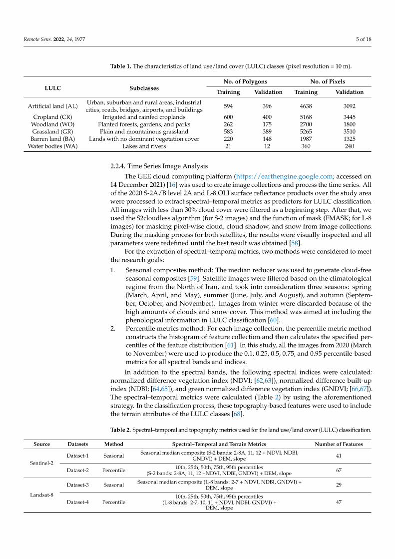
Table 1. The characteristics of land use/land cover (LULC) classes (pixel resolution = 10 m).

LULC SubclassesNo. of Polygons No. of Pixels

Training Validation Training Validation

Artificial land (AL) Urban, suburban and rural areas, industrialcities, roads, bridges, airports, and buildings 594 396 4638 3092

Cropland (CR) Irrigated and rainfed croplands 600 400 5168 3445Woodland (WO) Planted forests, gardens, and parks 262 175 2700 1800Grassland (GR) Plain and mountainous grassland 583 389 5265 3510

Barren land (BA) Lands with no dominant vegetation cover 220 148 1987 1325Water bodies (WA) Lakes and rivers 21 12 360 240

2.2.4. Time Series Image Analysis

The GEE cloud computing platform (https://earthengine.google.com; accessed on14 December 2021) [16] was used to create image collections and process the time series. Allof the 2020 S-2A/B level 2A and L-8 OLI surface reflectance products over the study areawere processed to extract spectral–temporal metrics as predictors for LULC classification.All images with less than 30% cloud cover were filtered as a beginning step. After that, weused the S2cloudless algorithm (for S-2 images) and the function of mask (FMASK; for L-8images) for masking pixel-wise cloud, cloud shadow, and snow from image collections.During the masking process for both satellites, the results were visually inspected and allparameters were redefined until the best result was obtained [58].

For the extraction of spectral–temporal metrics, two methods were considered to meetthe research goals:

1. Seasonal composites method: The median reducer was used to generate cloud-freeseasonal composites [59]. Satellite images were filtered based on the climatologicalregime from the North of Iran, and took into consideration three seasons: spring(March, April, and May), summer (June, July, and August), and autumn (Septem-ber, October, and November). Images from winter were discarded because of thehigh amounts of clouds and snow cover. This method was aimed at including thephenological information in LULC classification [60].

2. Percentile metrics method: For each image collection, the percentile metric methodconstructs the histogram of feature collection and then calculates the specified per-centiles of the feature distribution [61]. In this study, all the images from 2020 (Marchto November) were used to produce the 0.1, 0.25, 0.5, 0.75, and 0.95 percentile-basedmetrics for all spectral bands and indices.

In addition to the spectral bands, the following spectral indices were calculated:normalized difference vegetation index (NDVI; [62,63]), normalized difference built-upindex (NDBI; [64,65]), and green normalized difference vegetation index (GNDVI; [66,67]).The spectral–temporal metrics were calculated (Table 2) by using the aforementionedstrategy. In the classification process, these topography-based features were used to includethe terrain attributes of the LULC classes [68].

Table 2. Spectral–temporal and topography metrics used for the land use/land cover (LULC) classification.

Source Datasets Method Spectral–Temporal and Terrain Metrics Number of Features

Sentinel-2Dataset-1 Seasonal Seasonal median composite (S-2 bands: 2-8A, 11, 12 + NDVI, NDBI,

GNDVI) + DEM, slope 41

Dataset-2 Percentile 10th, 25th, 50th, 75th, 95th percentiles(S-2 bands: 2-8A, 11, 12 +NDVI, NDBI, GNDVI) + DEM, slope 67

Landsat-8

Dataset-3 Seasonal Seasonal median composite (L-8 bands: 2-7 + NDVI, NDBI, GNDVI) +DEM, slope 29

Dataset-4 Percentile10th, 25th, 50th, 75th, 95th percentiles

(L-8 bands: 2-7, 10, 11 + NDVI, NDBI, GNDVI) +DEM, slope

47

Remote Sens. 2022, 14, 1977 6 of 18

2.2.5. Land Cover Classification and Accuracy Assessment

A number of 2280 ground polygon samples (Section 2.2.3) were used to extract per-band pixel values of the four composited datasets. These samples were used to train the RFclassifier. RF is an ensemble learning method based on a combination of decision trees [69].This classifier was also found to perform better compared with other machine learning (ML)classifiers such as support vector machine (SVM) [70]. RF requires less processing time,fewer parameters, and minimal manual intervention compared with SVM [71,72]. It canalso cope properly with multi-modal data [73] and implicitly performs spectral selectiondue to its underlying principle [69]. Based on previous findings [74,75], a RF classifierwith 500 decision trees (i.e., ntree) was trained and tested on each dataset described inTable 2 to create LULC classifications. The assessment of classification accuracy was carriedout by comparing the LULC classes resulted from the training phase with data yieldedby the testing phase (numbers of ground polygon samples = 1520) using for this purposeconfusion matrices. Based on the confusion matrices, global quality metrics such as theoverall accuracy (OA) and kappa coefficient (K) were calculated (Equations (1) and (2)) toevaluate the impact of composition methods on LULC classification.

Overall Accuracy (OA) =Number of Correctly Classified Samples

Number of Total Samples(1)

Kappa =Overall Acuuracy− Estimated Chance Agreement

1− Estimated Chance Agreement(2)

Moreover, the class level consumer’s accuracy (CA), producer’s accuracy (PA), andF1-score were calculated (Equations (3)–(5)). The F1-score is the harmonic mean betweenproducer’s and user’s accuracies and can be used to evaluate the accuracy at class level [76].

CA =Number of Correctly Classified Samples in each Class

Number of Samples Classified to that Class(3)

PA =Number of Correctly Classified Samples in each ClassNumber of Samples from Reference Data in each Class

(4)

F1 =2×CA × PA

CA + PA(5)

PA is the probability that a pixel was correctly classified in a given class. CA is theprobability that a pixel classified in a given class of the map represents that class on theground [77]. The F1 was found to be the best performance metric and is widely used inprevious research, which gives equal importance to both PA (as a precision) and CA (as arecall) by combining them into a single model performance metric [78,79]. The methodologyadopted in this study is provided in the flowchart shown in Figure 2.

2.2.6. Variable Importance

Variable importance stands for the variables’ contribution to distinguish betweenLULC classes, which helps by improving the classification accuracy while reducing dataredundancy and processing workload. In this study, variable importance was derived fromthe RF model to estimate the contribution of variables (i.e., spectral bands and indices) tothe obtained accuracy of the model [80].

Remote Sens. 2022, 14, 1977 7 of 18Remote Sens. 2022, 14, x FOR PEER REVIEW 7 of 19

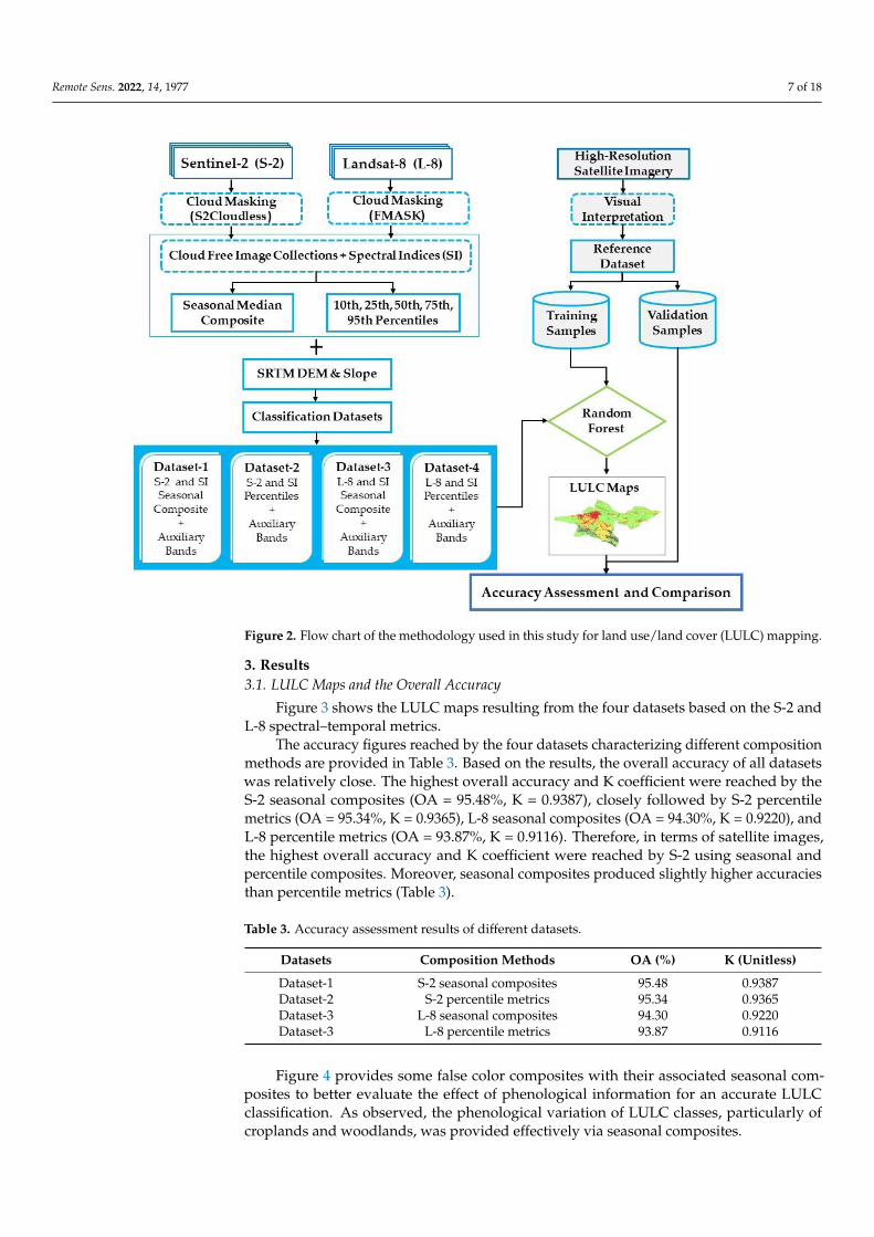
Figure 2. Flow chart of the methodology used in this study for land use/land cover (LULC) mapping.

2.2.6. Variable Importance

Variable importance stands for the variables’ contribution to distinguish between

LULC classes, which helps by improving the classification accuracy while reducing data

redundancy and processing workload. In this study, variable importance was derived

from the RF model to estimate the contribution of variables (i.e., spectral bands and indi-

ces) to the obtained accuracy of the model [80].

3. Results

3.1. LULC Maps and the Overall Accuracy

Figure 3 shows the LULC maps resulting from the four datasets based on the S-2 and

L-8 spectral–temporal metrics.

Figure 2. Flow chart of the methodology used in this study for land use/land cover (LULC) mapping.

3. Results3.1. LULC Maps and the Overall Accuracy

Figure 3 shows the LULC maps resulting from the four datasets based on the S-2 andL-8 spectral–temporal metrics.

The accuracy figures reached by the four datasets characterizing different compositionmethods are provided in Table 3. Based on the results, the overall accuracy of all datasetswas relatively close. The highest overall accuracy and K coefficient were reached by theS-2 seasonal composites (OA = 95.48%, K = 0.9387), closely followed by S-2 percentilemetrics (OA = 95.34%, K = 0.9365), L-8 seasonal composites (OA = 94.30%, K = 0.9220), andL-8 percentile metrics (OA = 93.87%, K = 0.9116). Therefore, in terms of satellite images,the highest overall accuracy and K coefficient were reached by S-2 using seasonal andpercentile composites. Moreover, seasonal composites produced slightly higher accuraciesthan percentile metrics (Table 3).

Table 3. Accuracy assessment results of different datasets.

Datasets Composition Methods OA (%) K (Unitless)

Dataset-1 S-2 seasonal composites 95.48 0.9387Dataset-2 S-2 percentile metrics 95.34 0.9365Dataset-3 L-8 seasonal composites 94.30 0.9220Dataset-3 L-8 percentile metrics 93.87 0.9116

Figure 4 provides some false color composites with their associated seasonal com-posites to better evaluate the effect of phenological information for an accurate LULCclassification. As observed, the phenological variation of LULC classes, particularly ofcroplands and woodlands, was provided effectively via seasonal composites.

Remote Sens. 2022, 14, 1977 8 of 18Remote Sens. 2022, 14, x FOR PEER REVIEW 8 of 19

Figure 3. Land use/land cover (LULC) maps of the study area resulting from: (a) S-2 seasonal com-

posites, (b) L-8 seasonal composites, (c) S-2 percentile metrics, and (d) L-8 percentile metrics.

The accuracy figures reached by the four datasets characterizing different composi-

tion methods are provided in Table 3. Based on the results, the overall accuracy of all

datasets was relatively close. The highest overall accuracy and K coefficient were reached

Figure 3. Land use/land cover (LULC) maps of the study area resulting from: (a) S-2 seasonalcomposites, (b) L-8 seasonal composites, (c) S-2 percentile metrics, and (d) L-8 percentile metrics.

Remote Sens. 2022, 14, 1977 9 of 18

Remote Sens. 2022, 14, x FOR PEER REVIEW 9 of 19

by the S-2 seasonal composites (OA = 95.48%, K = 0.9387), closely followed by S-2 percen-

tile metrics (OA = 95.34%, K = 0.9365), L-8 seasonal composites (OA = 94.30%, K = 0.9220),

and L-8 percentile metrics (OA = 93.87%, K = 0.9116). Therefore, in terms of satellite im-

ages, the highest overall accuracy and K coefficient were reached by S-2 using seasonal

and percentile composites. Moreover, seasonal composites produced slightly higher ac-

curacies than percentile metrics (Table 3).

Table 3. Accuracy assessment results of different datasets.

Datasets Composition Methods OA (%) K (Unitless)

Dataset-1 S-2 seasonal composites 95.48 0.9387

Dataset-2 S-2 percentile metrics 95.34 0.9365

Dataset-3 L-8 seasonal composites 94.30 0.9220

Dataset-3 L-8 percentile metrics 93.87 0.9116

Figure 4 provides some false color composites with their associated seasonal compo-

sites to better evaluate the effect of phenological information for an accurate LULC classi-

fication. As observed, the phenological variation of LULC classes, particularly of

croplands and woodlands, was provided effectively via seasonal composites.

Figure 4. Comparison of different seasonal composites. False-color images (R: near infrared (NIR),

G: red, and B: green) from Landsat-8 and Sentinel-2 time series. (a) Spring, (b) summer, and (c)

autumn.

3.2. Class Level Accuracy Assessment

For a more in-depth evaluation, per-class producer (PA) and consumer (CA) accura-

cies and F1-scores are provided for all datasets in Table 4. Regarding the role of time series

composition methods, for both S-2 and L-8 datasets, it can be observed that the CA, PA,

and F1 scores were higher in all LULC classes when using seasonal composites rather than

percentile metrics. The lowest CA, PA, and F1-score were calculated for bare lands and

the highest ones were observed for water bodies in all datasets.

Figure 4. Comparison of different seasonal composites. False-color images (R: near infrared(NIR), G: red, and B: green) from Landsat-8 and Sentinel-2 time series. (a) Spring, (b) summer,and (c) autumn.

3.2. Class Level Accuracy Assessment

For a more in-depth evaluation, per-class producer (PA) and consumer (CA) accuraciesand F1-scores are provided for all datasets in Table 4. Regarding the role of time seriescomposition methods, for both S-2 and L-8 datasets, it can be observed that the CA, PA,and F1 scores were higher in all LULC classes when using seasonal composites rather thanpercentile metrics. The lowest CA, PA, and F1-score were calculated for bare lands and thehighest ones were observed for water bodies in all datasets.

Table 4. Class level accuracy assessment results for all LULC classes (AL: artificial lands, WA: waterbodies, WO: woodland, CR: cropland, BA: bare land, and GR: grassland). Dataset-1: S-2 seasonalcomposites, dataset-2: S-2 percentile metrics, dataset-3: L-8 seasonal composites, and dataset-4: L-8percentile metrics.

Dataset Performance Metric AL WA WO CR BA GR

Dataset-1CA (%) 97.12 100.00 98.03 95.11 86.17 89.04PA (%) 98.13 100.00 93.18 96.01 81.06 94.11F1 (%) 97.62 100.00 95.54 95.55 83.53 91.50

Dataset-2CA (%) 97.01 99.02 97.11 95.02 84.17 91.09PA (%) 98.00 100.00 92.27 96.10 78.23 94.11F1 (%) 97.49 99.50 94.62 95.55 81.09 92.57

Dataset-3CA (%) 95.25 98.84 97.19 94.02 78.15 91.01PA (%) 98.11 100.00 93.09 94.11 74.32 92.20F1 (%) 96.65 99.44 95.09 94.06 76.18 91.09

Dataset-4CA (%) 95.01 97.05 97.01 94.09 78.06 90.32PA (%) 98.00 100.00 92.16 94.03 71.01 92.12F1 (%) 96.48 98.50 94.52 94.06 74.36 91.21

Remote Sens. 2022, 14, 1977 10 of 18

The highest CA, PA, and F1-scores for all LULC classes were produced by dataset-1(except grasslands). In contrast, dataset-4 had lower CA, PA, and F1 score values of allLULC classes (except grasslands). As observed in Table 4, the CA, PA, and F1 score valuesof artificial lands (AL) in all datasets were very high (F1-score ranged between 97.62 and94.48%) and there were no contrasting differences between different datasets. Similar resultswere also observed in terms of woodland (WO) classification (F1-score varied between95.54 and 94.52%), with the exception that PA values for all datasets were quite low (rangedbetween 93.18 and 92.16%). There were some omission errors in the woodland classification.Regarding the cropland (CR) classification, S-2 based datasets (seasonal composites andpercentiles metrics) achieved higher CA, PA, and F1-score values than the L-8 datasets.A similar difference in accuracy was observed by comparing the values returned by thecomposition methods used for each satellite time series. The F1-scores produced forcropland based on S-2 and L-8 datasets (seasonal and percentiles) were of 95.55 and 94.06%,respectively. Based on the results (Table 3), the lowest CA, PA, and F1-score values werecalculated for bare land in all datasets. The results also showed that the S-2 datasets had ahigher capability of mapping bare lands than L-8 datasets. For example, the CA and PAvalues produced for bare land using S-2 seasonal composites (dataset-1) increased by nearly8% and 7%, respectively, as opposed to L-8 seasonal composites (dataset-3). Moreover, animportant difference was observed in CA, PA, and F-1 scores of bare land classificationbetween these datasets. These differences were also observed between dataset-2 (S-2percentiles) and dataset-4 (L-8 percentiles). In terms of grassland classification, the bestresult was obtained with dataset-2, in which we used S-2 percentiles. But there were noremarkable differences between all datasets in grassland mapping accuracy.

Figure 5 provides some finer-scaled partitions of the maps to better evaluate the differ-ences between the datasets in identifying LULC classes. As shown, there were problemsin all datasets to distinguish between bare and artificial land, grassland, and harvestedcroplands, which remain challenging to differentiate due to similar spectral properties.

Remote Sens. 2022, 14, x FOR PEER REVIEW 11 of 19

Figure 5. Comparison between the classification results of different parts of the study area. (D-1) S-

2 seasonal composites, (D-2) S-2 percentile metrics, (D-3) L-8 seasonal composites, and (D-4) L-8

percentile metrics.

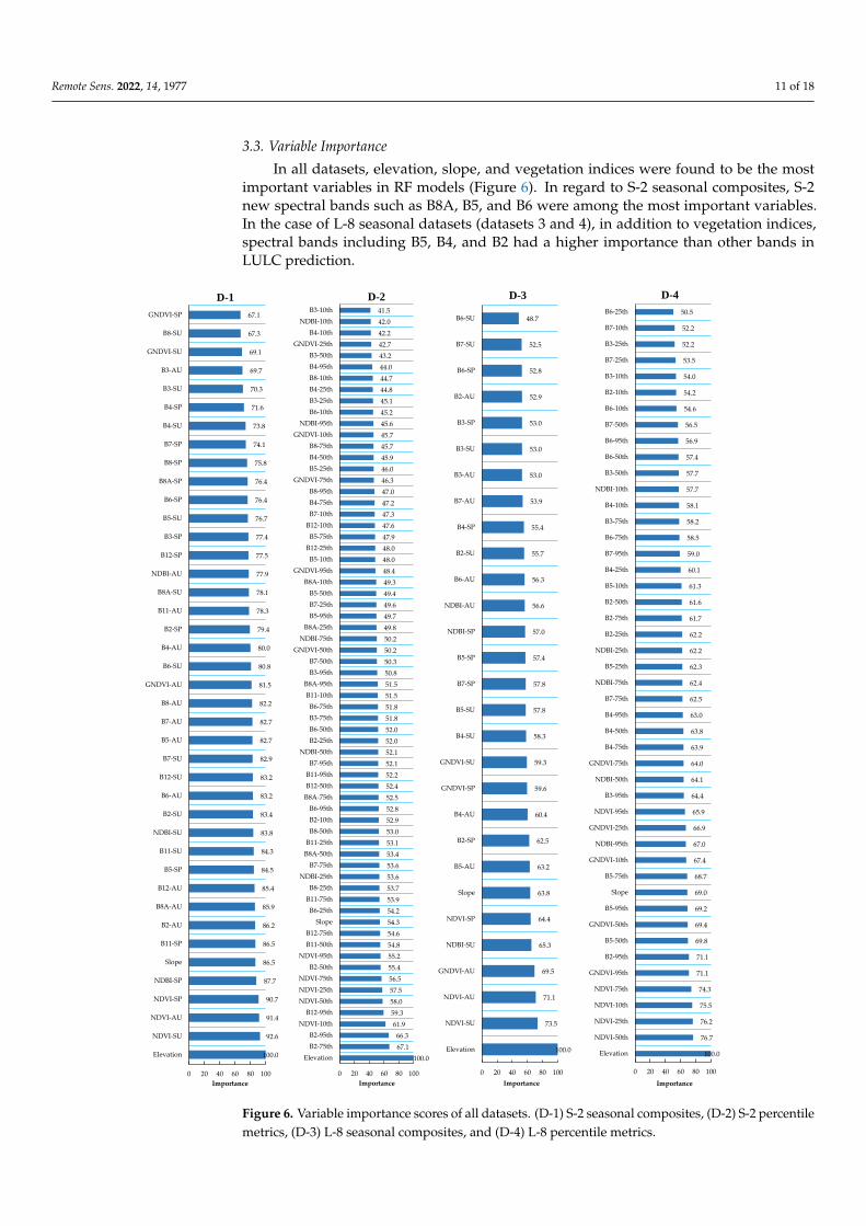
3.3. Variable Importance

In all datasets, elevation, slope, and vegetation indices were found to be the most

important variables in RF models (Figure 6). In regard to S-2 seasonal composites, S-2 new

spectral bands such as B8A, B5, and B6 were among the most important variables. In the

case of L-8 seasonal datasets (datasets 3 and 4), in addition to vegetation indices, spectral

bands including B5, B4, and B2 had a higher importance than other bands in LULC pre-

diction.

Figure 5. Comparison between the classification results of different parts of the study area. (D-1)S-2 seasonal composites, (D-2) S-2 percentile metrics, (D-3) L-8 seasonal composites, and (D-4) L-8percentile metrics.

Remote Sens. 2022, 14, 1977 11 of 18

3.3. Variable Importance

In all datasets, elevation, slope, and vegetation indices were found to be the mostimportant variables in RF models (Figure 6). In regard to S-2 seasonal composites, S-2new spectral bands such as B8A, B5, and B6 were among the most important variables.In the case of L-8 seasonal datasets (datasets 3 and 4), in addition to vegetation indices,spectral bands including B5, B4, and B2 had a higher importance than other bands inLULC prediction.

Remote Sens. 2022, 14, x FOR PEER REVIEW 12 of 19

Figure 6. Variable importance scores of all datasets. (D-1) S-2 seasonal composites, (D-2) S-2 percen-

tile metrics, (D-3) L-8 seasonal composites, and (D-4) L-8 percentile metrics.

100.0

92.6

91.4

90.7

87.7

86.5

86.5

86.2

85.9

85.4

84.5

84.3

83.8

83.4

83.2

83.2

82.9

82.7

82.7

82.2

81.5

80.8

80.0

79.4

78.3

78.1

77.9

77.5

77.4

76.7

76.4

76.4

75.8

74.1

73.8

71.6

70.3

69.7

69.1

67.3

67.1

0 20 40 60 80 100

Elevation

NDVI-SU

NDVI-AU

NDVI-SP

NDBI-SP

Slope

B11-SP

B2-AU

B8A-AU

B12-AU

B5-SP

B11-SU

NDBI-SU

B2-SU

B6-AU

B12-SU

B7-SU

B5-AU

B7-AU

B8-AU

GNDVI-AU

B6-SU

B4-AU

B2-SP

B11-AU

B8A-SU

NDBI-AU

B12-SP

B3-SP

B5-SU

B6-SP

B8A-SP

B8-SP

B7-SP

B4-SU

B4-SP

B3-SU

B3-AU

GNDVI-SU

B8-SU

GNDVI-SP

Importance

D-1

100.0

67.1

66.3

61.9

59.3

58.0

57.5

56.5

55.4

55.2

54.8

54.6

54.3

54.2

53.9

53.7

53.6

53.6

53.4

53.1

53.0

52.9

52.8

52.5

52.4

52.2

52.1

52.1

52.0

52.0

51.8

51.8

51.5

51.5

50.8

50.3

50.2

50.2

49.8

49.7

49.6

49.4

49.3

48.4

48.0

48.0

47.9

47.6

47.3

47.2

47.0

46.3

46.0

45.9

45.7

45.7

45.6

45.2

45.1

44.8

44.7

44.0

43.2

42.7

42.2

42.0

41.5

0 20 40 60 80 100

Elevation

B2-75th

B2-95th

NDVI-10th

B12-95th

NDVI-50th

NDVI-25th

NDVI-75th

B2-50th

NDVI-95th

B11-50th

B12-75th

Slope

B6-25th

B11-75th

B8-25th

NDBI-25th

B7-75th

B8A-50th

B11-25th

B8-50th

B2-10th

B6-95th

B8A-75th

B12-50th

B11-95th

B7-95th

NDBI-50th

B2-25th

B6-50th

B3-75th

B6-75th

B11-10th

B8A-95th

B3-95th

B7-50th

GNDVI-50th

NDBI-75th

B8A-25th

B5-95th

B7-25th

B5-50th

B8A-10th

GNDVI-95th

B5-10th

B12-25th

B5-75th

B12-10th

B7-10th

B4-75th

B8-95th

GNDVI-75th

B5-25th

B4-50th

B8-75th

GNDVI-10th

NDBI-95th

B6-10th

B3-25th

B4-25th

B8-10th

B4-95th

B3-50th

GNDVI-25th

B4-10th

NDBI-10th

B3-10th

Importance

D-2

100.0

73.5

71.1

69.5

65.3

64.4

63.8

63.2

62.5

60.4

59.6

59.3

58.3

57.8

57.8

57.4

57.0

56.6

56.3

55.7

55.4

53.9

53.0

53.0

53.0

52.9

52.8

52.5

48.7

0 20 40 60 80 100

Elevation

NDVI-SU

NDVI-AU

GNDVI-AU

NDBI-SU

NDVI-SP

Slope

B5-AU

B2-SP

B4-AU

GNDVI-SP

GNDVI-SU

B4-SU

B5-SU

B7-SP

B5-SP

NDBI-SP

NDBI-AU

B6-AU

B2-SU

B4-SP

B7-AU

B3-AU

B3-SU

B3-SP

B2-AU

B6-SP

B7-SU

B6-SU

Importance

D-3

100.0

76.7

76.2

75.5

74.3

71.1

71.1

69.8

69.4

69.2

69.0

68.7

67.4

67.0

66.9

65.9

64.4

64.1

64.0

63.9

63.8

63.0

62.5

62.4

62.3

62.2

62.2

61.7

61.6

61.3

60.1

59.0

58.5

58.2

58.1

57.7

57.7

57.4

56.9

56.5

54.6

54.2

54.0

53.5

52.2

52.2

50.5

0 20 40 60 80 100

Elevation

NDVI-50th

NDVI-25th

NDVI-10th

NDVI-75th

GNDVI-95th

B2-95th

B5-50th

GNDVI-50th

B5-95th

Slope

B5-75th

GNDVI-10th

NDBI-95th

GNDVI-25th

NDVI-95th

B3-95th

NDBI-50th

GNDVI-75th

B4-75th

B4-50th

B4-95th

B7-75th

NDBI-75th

B5-25th

NDBI-25th

B2-25th

B2-75th

B2-50th

B5-10th

B4-25th

B7-95th

B6-75th

B3-75th

B4-10th

NDBI-10th

B3-50th

B6-50th

B6-95th

B7-50th

B6-10th

B2-10th

B3-10th

B7-25th

B3-25th

B7-10th

B6-25th

Importance

D-4

Figure 6. Variable importance scores of all datasets. (D-1) S-2 seasonal composites, (D-2) S-2 percentilemetrics, (D-3) L-8 seasonal composites, and (D-4) L-8 percentile metrics.

Remote Sens. 2022, 14, 1977 12 of 18

4. Discussion

Spatial distribution of LULC classes is often related to topographic factors [9,81].Therefore, we considered elevation and slope factors in training and testing the RF models.As a result, in all RF models, elevation factors obtained high importance scores. Theimportance of topographic variables in large-scale LULC classification was also reported insimilar studies [39,82]. For example, Rufin et al. [83] used topographic factors (elevationand slope) in their LULC model and indicate their high importance in increasing the overallaccuracy. In another study, Htitiou et al. [30] used elevation and slope layers in the attemptto map croplands at national scale. Based on their results, these variables improved theability to distinguish croplands, particularly in regions characterized by high elevation andsteep slopes. Phan et al. [84] defined several datasets based on L-8 time series and auxiliarybands such as topographic factors and reported that the elevation was the most importantvariable in all of the models. Therefore, the high importance of topographic factors used inthis study was consistent with the results reported by previous studies.

Regarding the composition methods used for S-2 and L-8 time series, the resultsshowed that seasonal composites outperformed percentile metrics in distinguishing dif-ferent LULC classes. In terms of accurate LULC mapping, the strategy used to generatecomposites depends on the types of LULC classes and the density of available time se-ries [44]. The higher performance of seasonal composites in this study can be related tothe selected LULC classes which covered cropland, woodland, and grassland. The use ofseasonal composites enabled the inclusion of phenological information. These kinds of sea-sonality features were a piece of sufficient and valuable information for distinguishing theLULC classes with similar spectral attributes. The importance of phenological informationwas also reported in similar studies. Xie et al. [44] defined two datasets based on monthlymedian composites and percentile metrics to classify different LULC classes including vari-ous types of vegetation such as evergreen forests, deciduous forests, shrublands, croplands,etc., using Landsat TM/ETM+ time series and reported that the highest overall accuracywas produced by using monthly median composites.

When comparing the two satellite time series, accuracy assessment results indicatedthat S-2 composition methods (seasonal composites and percentiles metrics) producedhigher accuracies than their L-8 counterparts did. The L-8 time series used in this study hadsimilar spectral features to S-2 time series, excluding the red-edge bands of S-2. Therefore,the better results provided by the S-2 could be related to the red-edge bands and theirspectral–temporal metrics. The feasibility and efficiency of red-edge bands were alsopresent in variable importance scores. As Figure 6 illustrates, in both seasonal and percentilecomposites, red edge bands (B-7, 6, and 5) played a significant role in the performance of theRF classifier. Forkuor et al. [85] defined several datasets with different feature configurationsbased on mono date S-2 and L-8 bands. Based on their results, the S-2 dataset produced thehighest accuracy. To evaluate the effect of red edge bands on the classification results, theyalso added S-2 red edge bands to the L-8 dataset and reported a 4% improvement comparedwith L-8 bands. Moreover, Immitzer et al. [86] reported that red-edge bands, particularlyB-5 (RE1), are among the most important data features in mapping vegetation types suchas croplands and woodlands. Ghayour et al. [87] compared the performance of S-2 andL-8 satellite images in LULC mapping by using classifiers such as SVM, artificial neuralnetwork (ANN), maximum likelihood classification (MLC), minimum distance (MD), andMahalanobis distance (MHD). According to their findings, S-2 produced higher accuraciescompared with the L-8 datasets irrespective of the classifier used.

Analyzing the confusion matrices indicated that bare lands were poorly identifiedand most of them were classified as grasslands. Moreover, some pixels of the bare landwere misclassified as artificial lands. This problem occurred more often in the L-8 baseddatasets (dataset-3 and dataset-4). Therefore, the largest difference between the S-2 andL-8 composites was that observed in the classification of bare lands. The classification ofbare lands, on the other hand, is a common challenge in LULC mapping studies. Zhaoand Zhu [88] reported that some LULC classes such as artificial lands, bare lands, deserts,

Remote Sens. 2022, 14, 1977 13 of 18

and harvested croplands have similar spectral signatures and tried to develop a spectralindex to better distinguish these classes. They introduced the artificial surface index (ASI)by considering the artificial surface enhancement, vegetation, and bare soil suppressingand reported that ASI could increase the separability of artificial lands from other types ofland use. Ettehadi Osgouei et al. [89] faced the same challenge and tried to use spectralindices, including the normalized difference tillage index (NDTI), red-edge based NDVI,and modified normalized difference water index (MNDWI). They reported that thesespectral indices could improve the performance of the SVM classifier to distinguish bareland from urban areas. We used similar spectral indices in this study, including the NDVI,GNDVI, and NDBI, but it seems that this challenge still remains. Nevertheless, thesespectral indices showed a good performance in differentiating other classes with similarspectral signatures, such as woodland and dense croplands.

In this study, croplands were composed of irrigated and rain-fed crops, which holdheterogeneous spectral patterns [90]. Considering all these spectral similarities and hetero-geneous patterns, our approach and the used spectral–temporal metrics could enhance theclassification accuracy. In some studies, the integrated use of textural and spectral featureswas found to be a solution to distinguish LULC classes with similar spectral properties.For example, Petrushevsky et al. [91] integrated S-2 multispectral bands, Sentinel-1 texturefeatures, and object-based image analysis to generate an urban mask and reached a 90%overall accuracy. The radar signal is sensitive to geometry (e.g., roughness, texture, andinternal structure), while physiology influences optical reflectance [92]. As such, these twospectral domains may provide complementary information [93]. Hence, the integration ofradar time series and textural feature is recommended for future research [94,95].

Under the GEE platform, the satellite image processing time can be greatly shortened,which helps users to store decades of data and removes the need to download the satelliteimages one by one. However, one of the limitations of our study was the limited availabilityof data with suitable resolution in the Google Earth catalog, whose improvement in thisdirection is desirable for both researchers and practitioners. The second limitation of thisstudy was the lack of precise training and validation samples, making it impossible for usto conduct our study on a much larger scale. These samples were collected automaticallyfrom existing reference datasets such as the land use/cover area frame survey (LUCAS)in similar studies. There was no access to accurate reference datasets or reliable LULCmaps in our study area. Therefore, we used very high resolution (VHR) satellite imagesprovided by Google Earth and visual interpretation, which are very time-consuming andchallenging, particularly when dealing with large areas. Moreover, based on the previousstudies and our results, topographic bands (such as elevation and slope) are very importantvariables in increasing the overall accuracy. In this study, we used freely available SRTMDEM with a resolution of approximately 30 m. Considering the importance of topographicvariables, using more accurate DEMs could considerably increase the classification results.Unfortunately, we didn’t have access to such high-resolution DEM in this study (thirdlimitation). Therefore, future studies could use more accurate DEM, especially whendealing with mountainous landscapes. Future research may compare the existing land useproducts, such as those from this paper, with global products (e.g., ESA WorldCover andGlobCover maps). Since the classification accuracy may be affected by the type of machinelearning model used, future studies could compare the results of other popular classifiersfor LULC mapping such as SVM, ANN, and deep learning models. Finally, we suggestcomparing balanced and imbalanced reference datasets in terms of classification accuracyas well as considering larger study areas with different climate conditions.

5. Conclusions

This study aimed at evaluating the potential of S-2 and L-8 time series and the RFclassifier to produce accurate LULC maps. The S-2 and L-8 time series were used to generatespectral–temporal metrics based on two composition methods (seasonal and percentiles) toachieve the research objectives. Datasets, including S-2 and L-8 spectral temporal metrics

Remote Sens. 2022, 14, 1977 14 of 18

and vegetation indices were defined, then their performance in identifying six commonLULC classes (artificial land, water bodies, woodland, cropland, bare land, and grassland)was compared. The study concludes that medium resolution satellite time series andthe extracted spectral–temporal metrics are robust sources for accurate LULC mapping.However, some differences among the datasets were observed. For instance, the LULCmaps generated from the S-2 time series were more accurate than those generated fromthe L-8 time series. The comparison between composition methods indicated that seasonalmedian composites outperformed percentile metrics in both S-2 and L-8 time series. Theresults proved the efficiency of vegetation indices, particularly of NDVI and NDBI andS-2 red-edge bands, concerning the variable importance. In short, the approach used inthis research and the generated spectral–temporal metrics can be used to produce accurateLULC maps based on the GEE cloud computing platform. These results highlight thatcloud computing platforms such as GEE and new Earth-observing satellites such as S-2have contributed significantly in improving LULC mapping and monitoring.

Author Contributions: Conceptualization, V.N., A.D., F.M. and S.M.M.S.; data curation, V.N. andA.D.; formal analysis, V.N., A.D. and F.M.; funding acquisition, A.D., S.M.M.S. and S.A.B.; inves-tigation, V.N.; methodology, V.N., A.D., F.M. and S.M.M.S.; software, V.N. and A.D.; supervision,A.D. and S.M.M.S.; visualization, V.N. and S.M.M.S.; writing—original draft, V.N.; writing—reviewand editing, A.D., S.M.M.S. and S.A.B. All authors have read and agreed to the published version ofthe manuscript.

Funding: This research received no external funding and the APC was funded by the Department ofForest Engineering, Forest Management Planning, and Terrestrial Measurements.

Data Availability Statement: The data supporting the findings of this study are available from thefirst author (V.N.) upon reasonable request.

Acknowledgments: Azade Deljouei’s and Seyed Mohammad Moein Sadeghi’s research at the Tran-silvania University of Brasov, Romania, was supported by the program “Transilvania Fellowship forPostdoctoral Research/Young Researchers”.

Conflicts of Interest: The authors declare no conflict of interest.

Abbreviations

The following abbreviations are used in this manuscript:

AL Artificial landANN Artificial neural networkASI Artificial surface indexBA Barren landCA Consumer’s accuracyCR CroplandDEM Digital elevation modelFMASK Function of maskFORCE Framework for Operational Radiometric Correction for Environmental monitoringGEE Google Earth EngineGNDVI Green normalized difference vegetation indexGR GrasslandK Kappa coefficientL-8 Landsat-8LULC Land use and land coverLUCAS Land use/cover area frame surveyMD Minimum distanceMHD Mahalanobis distanceMLC Maximum likelihood classificationMNDWI Modified normalized difference water indexNASA National Aeronautics and Space AdministrationNGA National Geospatial-Intelligence Agency

Remote Sens. 2022, 14, 1977 15 of 18

NIR Near infraredNDBI Normalized difference built-up indexNDTI Normalized difference tillage indexNDVI Normalized difference vegetation indexOA Overall accuracyOLI Operational Land ImagerPA Producer’s accuracyRF Random forestS-2 Sentinel-2SRTM Shuttle radar topography missionSSE Space Shuttle EndeavourSVM Support vector machineSWIR Short-wave infraredVHR Very high resolutionWA Water bodiesWO Woodland

References1. Esfandeh, S.; Danehkar, A.; Salmanmahiny, A.; Sadeghi, S.M.M.; Marcu, M.V. Climate Change Risk of Urban Growth and Land

Use/Land Cover Conversion: An In-Depth Review of the Recent Research in Iran. Sustainability 2021, 14, 338. [CrossRef]2. Yao, Y.; Yan, X.; Luo, P.; Liang, Y.; Ren, S.; Hu, Y.; Han, J.; Guan, Q. Classifying Land-Use Patterns by Integrating Time-Series

Electricity Data and High-Spatial Resolution Remote Sensing Imagery. Int. J. Appl. Earth Observ. Geoinf. 2022, 106, 102664.[CrossRef]

3. Qian, X.; Zhang, L. An Integration Method to Improve the Quality of Global Land Cover. Adv. Space Res. 2022, 69, 1427–1438.[CrossRef]

4. Schulz, D.; Yin, H.; Tischbein, B.; Verleysdonk, S.; Adamou, R.; Kumar, N. Land Use Mapping Using Sentinel-1 and Sentinel-2Time Series in a Heterogeneous Landscape in Niger, Sahel. ISPRS J. Photogramm. Remote Sens. 2021, 178, 97–111. [CrossRef]

5. Viana, C.M.; Girão, I.; Rocha, J. Long-Term Satellite Image Time-series for land use/land cover change detection using refinedopen source data in a rural region. Remote Sens. 2019, 11, 1104. [CrossRef]

6. Praticò, S.; Solano, F.; Di Fazio, S.; Modica, G. Machine Learning Classification of Mediterranean Forest Habitats in GoogleEarth Engine Based on Seasonal Sentinel-2 Time-Series and Input Image Composition Optimisation. Remote Sens. 2021, 13, 586.[CrossRef]

7. Sobhani, P.; Esmaeilzadeh, H.; Barghjelveh, S.; Sadeghi, S.M.M.; Marcu, M.V. Habitat Integrity in Protected Areas Threatened byLULC Changes and Fragmentation: A Case Study in Tehran Province, Iran. Land 2021, 11, 6. [CrossRef]

8. Steinhausen, M.J.; Wagner, P.D.; Narasimhan, B.; Waske, B. Combining Sentinel-1 and Sentinel-2 Data for Improved Land Useand Land Cover Mapping of Monsoon Regions. Int. J. Appl. Earth Observ. Geoinf. 2018, 73, 595–604. [CrossRef]

9. Kupidura, P. The Comparison of Different Methods of Texture Analysis for Their Efficacy for Land Use Classification in SatelliteImagery. Remote Sens. 2019, 11, 1233. [CrossRef]

10. Wang, D.; Wan, B.; Qiu, P.; Tan, X.; Zhang, Q. Mapping Mangrove Species Using Combined UAV-LiDAR and Sentinel-2 Data:Feature Selection and Point Density Effects. Adv. Space Res. 2022, 69, 1494–1512. [CrossRef]

11. Ienco, D.; Interdonato, R.; Gaetano, R.; Minh, D.H.T. Combining Sentinel-1 and Sentinel-2 Satellite Image Time Series for LandCover Mapping Via a Multi-Source Deep Learning Architecture. ISPRS J. Photogramm. Remote Sens. 2019, 158, 11–22. [CrossRef]

12. Sun, B.; Zhang, Y.; Zhou, Q.; Zhang, X. Effectiveness of Semi-Supervised Learning and Multi-Source Data in Detailed UrbanLanduse Mapping with a Few Labeled Samples. Remote Sens. 2022, 14, 648. [CrossRef]

13. Clerici, N.; Valbuena Calderón, C.A.; Posada, J.M. Fusion of Sentinel-1A and Sentinel-2A Data for Land Cover Mapping: A CaseStudy in the Lower Magdalena Region, Colombia. J. Maps 2017, 13, 718–726. [CrossRef]

14. Sudmanns, M.; Tiede, D.; Augustin, H.; Lang, S. Assessing Global Sentinel-2 Coverage Dynamics and Data Availability forOperational Earth Observation (EO) Applications Using the EO-Compass. Int. J. Digital Earth 2020, 13, 768–784. [CrossRef][PubMed]

15. Wulder, M.A.; White, J.C.; Loveland, T.R.; Woodcock, C.E.; Belward, A.S.; Cohen, W.B.; Fosnight, E.A.; Shaw, J.; Masek, J.G.;Roy, D.P. The Global Landsat Archive: Status, Consolidation, and Direction. Remote Sens. Environ. 2016, 185, 271–283. [CrossRef]

16. Gorelick, N.; Hancher, M.; Dixon, M.; Ilyushchenko, S.; Thau, D.; Moore, R. Google Earth Engine: Planetary-Scale GeospatialAnalysis for Everyone. Remote Sens. Environ. 2017, 202, 18–27. [CrossRef]

17. Guo, J.; Huang, C.; Hou, J. A Scalable Computing Resources System for Remote Sensing Big Data Processing Using GeoPySparkBased on Spark on K8s. Remote Sens. 2022, 14, 521. [CrossRef]

18. Kempeneers, P.; Kliment, T.; Marletta, L.; Soille, P. Parallel Processing Strategies for Geospatial Data in a Cloud ComputingInfrastructure. Remote Sens. 2022, 14, 398. [CrossRef]

19. Cooper, S.; Okujeni, A.; Pflugmacher, D.; van der Linden, S.; Hostert, P. Combining Simulated Hyperspectral EnMAP and LandsatTime Series for Forest Aboveground Biomass Mapping. Int. J. Appl. Earth Observ. Geoinf. 2021, 98, 102307. [CrossRef]

Remote Sens. 2022, 14, 1977 16 of 18

20. Xu, L.; Herold, M.; Tsendbazar, N.-E.; Masiliunas, D.; Li, L.; Lesiv, M.; Fritz, S.; Verbesselt, J. Time Series Analysis for Global LandCover Change Monitoring: A Comparison Across Sensors. Remote Sens. Environ. 2022, 271, 112905. [CrossRef]

21. Lary, D.J.; Alavi, A.H.; Gandomi, A.H.; Walker, A.L. Machine Learning in Geosciences and Remote Sensing. Geosci. Front. 2016, 7,3–10. [CrossRef]

22. Maxwell, A.E.; Warner, T.A.; Fang, F. Implementation of Machine-Learning Classification in Remote Sensing: An Applied Review.Int. J. Remote Sens. 2018, 39, 2784–2817. [CrossRef]

23. Kwan, C.; Ayhan, B.; Budavari, B.; Lu, Y.; Perez, D.; Li, J.; Bernabe, S.; Plaza, A. Deep Learning for Land Cover ClassificationUsing Only a Few Bands. Remote Sens. 2020, 12, 2000. [CrossRef]

24. Naushad, R.; Kaur, T.; Ghaderpour, E. Deep Transfer Learning for Land Use and Land Cover Classification: A Comparative Study.Sensors 2021, 21, 8083. [CrossRef]

25. Sefrin, O.; Riese, F.M.; Keller, S. Deep Learning for Land Cover Change Detection. Remote Sens. 2020, 13, 78. [CrossRef]26. Frantz, D. FORCE—Landsat+ Sentinel-2 Analysis Ready Data and Beyond. Remote Sens. 2019, 11, 1124. [CrossRef]27. Tassi, A.; Vizzari, M. Object-Oriented LULC Classification in Google Earth Engine Combining SNICc, GLCM, and Machine

Learning Algorithms. Remote Sens. 2020, 12, 3776. [CrossRef]28. Kumar, L.; Mutanga, O. Google Earth Engine Applications Since Inception: Usage, Trends, and Potential. Remote Sens. 2018,

10, 1509. [CrossRef]29. Carrasco, L.; O’Neil, A.W.; Morton, R.D.; Rowland, C.S. Evaluating Combinations of Temporally Aggregated Sentinel-1, Sentinel-2

and Landsat 8 for Land Cover Mapping with Google Earth Engine. Remote Sens. 2019, 11, 288. [CrossRef]30. Htitiou, A.; Boudhar, A.; Chehbouni, A.; Benabdelouahab, T. National-Scale Cropland Mapping Based on Phenological Metrics,

Environmental Covariates, and Machine Learning on Google Earth Engine. Remote Sens. 2021, 13, 4378. [CrossRef]31. Liang, S.; Gong, Z.; Wang, Y.; Zhao, J.; Zhao, W. Accurate Monitoring of Submerged Aquatic Vegetation in a Macrophytic Lake

Using Time-Series Sentinel-2 Images. Remote Sens. 2022, 14, 640. [CrossRef]32. Zhou, Q.; Zhu, Z.; Xian, G.; Li, C. A Novel Regression Method for Harmonic Analysis of Time Series. ISPRS J. Photogramm. Remote

Sens. 2022, 185, 48–61. [CrossRef]33. Luo, C.; Zhang, X.; Wang, Y.; Men, Z.; Liu, H. Regional Soil Organic Matter Mapping Models Based on the Optimal Time Window,

Feature Selection Algorithm and Google Earth Engine. Soil Tillage Res. 2022, 219, 105325. [CrossRef]34. Okujeni, A.; Canters, F.; Cooper, S.D.; Degerickx, J.; Heiden, U.; Hostert, P.; Priem, F.; Roberts, D.A.; Somers, B.; van der Linden, S.

Generalizing Machine Learning Regression Models Using Multi-Site Spectral Libraries for Mapping Vegetation-Impervious-SoilFractions Across Multiple Cities. Remote Sens. Environ. 2018, 216, 482–496. [CrossRef]

35. Kowalski, K.; Okujeni, A.; Brell, M.; Hostert, P. Quantifying Drought Effects in Central European Grasslands Through Regression-Based Unmixing of Intra-Annual Sentinel-2 Time Series. Remote Sens. Environ. 2022, 268, 112781. [CrossRef]

36. Liu, L.; Xiao, X.; Qin, Y.; Wang, J.; Xu, X.; Hu, Y.; Qiao, Z. Mapping Cropping Intensity in China Using Time Series Landsat andSentinel-2 Images and Google Earth Engine. Remote Sens. Environ. 2020, 239, 111624. [CrossRef]

37. Hermosilla, T.; Wulder, M.A.; White, J.C.; Coops, N.C.; Hobart, G.W. Disturbance-Informed Annual Land Cover ClassificationMaps of Canada’s Forested Ecosystems for a 29-Year Landsat Time Series. Can. J. Remote Sens. 2018, 44, 67–87. [CrossRef]

38. Yuan, Y.; Lin, L.; Liu, Q.; Hang, R.; Zhou, Z.-G. SITS-Former: A Pre-Trained Spatio-Spectral-Temporal Representation Model forSentinel-2 Time Series Classification. Int. J. Appl. Earth Observ. Geoinf. 2022, 106, 102651. [CrossRef]

39. Pflugmacher, D.; Rabe, A.; Peters, M.; Hostert, P. Mapping Pan-European Land Cover Using Landsat Spectral-Temporal Metricsand the European LUCAS Survey. Remote Sens. Environ. 2019, 221, 583–595. [CrossRef]

40. White, J.C.; Hermosilla, T.; Wulder, M.A.; Coops, N.C. Mapping, Validating, and Interpreting Spatio-Temporal Trends inPost-Disturbance Forest Recovery. Remote Sens. Environ. 2022, 271, 112904. [CrossRef]

41. Salinero-Delgado, M.; Estévez, J.; Pipia, L.; Belda, S.; Berger, K.; Paredes Gómez, V.; Verrelst, J. Monitoring Cropland Phenologyon Google Earth Engine Using Gaussian Process Regression. Remote Sens. 2021, 14, 146. [CrossRef]

42. Azzari, G.; Lobell, D. Landsat-based classification in the cloud: An opportunity for a paradigm shift in land cover monitoring.Remote Sens. Environ. 2017, 202, 6474. [CrossRef]

43. Hemmerling, J.; Pflugmacher, D.; Hostert, P. Mapping Temperate Forest Tree Species Using Dense Sentinel-2 Time Series. RemoteSens. Environ. 2021, 267, 112743. [CrossRef]

44. Xie, S.; Liu, L.; Zhang, X.; Yang, J.; Chen, X.; Gao, Y. Automatic Land-Cover Mapping Using Landsat Time-Series Data Based onGoogle Earth Engine. Remote Sens. 2019, 11, 3023. [CrossRef]

45. Lan, H.; Stewart, K.; Sha, Z.; Xie, Y.; Chang, S. Data Gap Filling Using Cloud-Based Distributed Markov Chain Cellular AutomataFramework for Land Use and Land Cover Change Analysis: Inner Mongolia as a Case Study. Remote Sens. 2022, 14, 445.[CrossRef]

46. Stromann, O.; Nascetti, A.; Yousif, O.; Ban, Y. Dimensionality Reduction and Feature Selection for Object-Based Land CoverClassification Based on Sentinel-1 and Sentinel-2 Time Series Using Google Earth Engine. Remote Sens. 2019, 12, 76. [CrossRef]

47. Masolele, R.N.; De Sy, V.; Herold, M.; Marcos, D.; Verbesselt, J.; Gieseke, F.; Mullissa, A.G.; Martius, C. Spatial and TemporalDeep Learning Methods for Deriving Land-Use Following Deforestation: A Pan-Tropical Case Study Using Landsat Time Series.Remote Sens. Environ. 2021, 264, 112600. [CrossRef]

48. Santos, L.A.; Ferreira, K.; Picoli, M.; Camara, G.; Zurita-Milla, R.; Augustijn, E.-W. Identifying Spatiotemporal Patterns in LandUse and Cover Samples from Satellite Image Time Series. Remote Sens. 2021, 13, 974. [CrossRef]

Remote Sens. 2022, 14, 1977 17 of 18

49. Thonfeld, F.; Steinbach, S.; Muro, J.; Kirimi, F. Long-Term Land Use/Land Cover Change Assessment of the Kilombero Catchmentin Tanzania Using Random Forest Classification and Robust Change Vector Analysis. Remote Sens. 2020, 12, 1057. [CrossRef]

50. Heshmatol Vaezin, S.M.; Moftakhar Juybari, M.; Daei, A.; Avatefi Hemmat, M.; Shirvany, A.; Tallis, M.J.; Hirabayashi, S.;Moeinaddini, M.; Hamidian, A.H.; Sadeghi, S.M.M.; et al. The Effectiveness of Urban Trees in Reducing Airborne ParticulateMatter by Dry Deposition in Tehran, Iran. Env. Mon. Assess. 2021, 193, 842. [CrossRef]

51. Hidalgo, D.R.; Cortés, B.B.; Bravo, E.C. Dimensionality Reduction of Hyperspectral Images of Vegetation and Crops Based onSelf-Organized Maps. Inf. Process. Agricul. 2021, 8, 310–327. [CrossRef]

52. Tu, T.-M.; Chen, C.-H.; Wu, J.-L.; Chang, C.-I. A Fast Two-stage Classification Method for High-Dimensional Remote SensingData. IEEE Trans. Geosci. Remote Sens. 1998, 36, 182–191.

53. McCarty, D.A.; Kim, H.W.; Lee, H.K. Evaluation of Light Gradient Boosted Machine Learning Technique in Large Scale Land Useand Land Cover Classification. Environments 2020, 7, 84. [CrossRef]

54. Li, W.; Dong, R.; Fu, H.; Wang, J.; Yu, L.; Gong, P. Integrating Google Earth Imagery with Landsat Data to Improve 30-mResolution Land Cover Mapping. Remote Sens. Environ. 2020, 237, 111563. [CrossRef]

55. Yang, D.; Fu, C.-S.; Smith, A.C.; Yu, Q. Open Land-Use Map: A Regional Land-Use Mapping Strategy for IncorporatingOpenStreetMap with Earth Observations. Geo-Spatial Inf. Sci. 2017, 20, 269–281. [CrossRef]

56. Colditz, R.R. An Evaluation of Different Training Sample Allocation Schemes for Discrete and Continuous Land Cover Classifica-tion Using Decision Tree-Based Algorithms. Remote Sens. 2015, 7, 9655–9681. [CrossRef]

57. Thanh Noi, P.; Kappas, M. Comparison of Random Forest, k-Nearest Neighbor, and Support Vector Machine Classifiers for andCover Classification Using Sentinel-2 Imagery. Sensors 2017, 18, 18. [CrossRef]

58. Li, J.; Wang, L.; Liu, S.; Peng, B.; Ye, H. An Automatic Cloud Detection Model for Sentinel-2 Imagery Based on Google EarthEngine. Remote Sens. Lett. 2022, 13, 196–206. [CrossRef]

59. Tsai, Y.H.; Stow, D.; Chen, H.L.; Lewison, R.; An, L.; Shi, L. Mapping Vegetation and Land Use Types in Fanjingshan NationalNature Reserve Using Google Earth Engine. Remote Sens. 2018, 10, 927. [CrossRef]

60. Xu, Y.; Yu, L.; Zhao, F.R.; Cai, X.; Zhao, J.; Lu, H.; Gong, P. Tracking Annual Cropland Changes from 1984 to 2016 UsingTime-Series Landsat Images with a Change-Detection and Post-Classification Approach: Experiments from Three Sites in Africa.Remote Sens. Environ. 2018, 218, 13–31. [CrossRef]

61. Gong, P.; Wang, J.; Yu, L.; Zhao, Y.; Zhao, Y.; Liang, L.; Niu, Z.; Huang, X.; Fu, H.; Liu, S. Finer Resolution Observation andMonitoring of Global Land Cover: First Mapping Results with Landsat TM and ETM+ data. Int. J. Remote Sens. 2013, 34,2607–2654. [CrossRef]

62. Nasiri, V.; Darvishsefat, A.A.; Arefi, H.; Griess, V.C.; Sadeghi, S.M.M.; Borz, S.A. Modeling Forest Canopy Cover: A SynergisticUse of Sentinel-2, Aerial Photogrammetry Data, and Machine Learning. Remote Sens. 2022, 14, 1453. [CrossRef]

63. Rouse, J.W.; Haas, R.H.; Schell, J.A.; Deering, D.W. Monitoring the Vernal Advancement and Retrogradation (Green Wave Effect)of Natural Vegetation. Prog. Rep. RSC 1978–1. 1973. Available online: https://core.ac.uk/download/pdf/42887948.pdf (accessedon 17 December 2021).

64. Kulkarni, K.; Vijaya, P. NDBI Based Prediction of Land Use Land Cover Change. J. Indian Soc. Remote Sens. 2021, 49, 2523–2537.[CrossRef]

65. Zha, Y.; Gao, J.; Ni, S. Use of Normalized Difference Built-Up Index in Automatically Mapping Urban Areas from TM Imagery.Int. J. Remote Sens. 2003, 24, 583–594. [CrossRef]

66. Buschmann, C.; Nagel, E. In Vivo Spectroscopy and Internal Optics of Leaves as Basis for Remote Sensing of Vegetation. Int. J.Remote Sens. 1993, 14, 711–722. [CrossRef]

67. Gitelson, A.A.; Merzlyak, M.N. Remote Sensing of Chlorophyll Concentration in Higher Plant Leaves. Adv. Space Res. 1998, 22,689–692. [CrossRef]

68. Brandt, J.S.; Townsend, P.A. Land Use–Land Cover Conversion, Regeneration and Degradation in the High Elevation BolivianAndes. Landsc. Ecol. 2006, 21, 607–623. [CrossRef]

69. Breiman, L. Random Forests. Mach. Learn. 2001, 45, 5–32. [CrossRef]70. Sheykhmousa, M.; Mahdianpari, M.; Ghanbari, H.; Mohammadimanesh, F.; Ghamisi, P.; Homayouni, S. Support Vector Machine

Versus Random Forest for Remote Sensing Image Classification: A Meta-Analysis and Systematic Review. IEEE J. Sel. Top. Appl.Earth Observ. Remote Sens. 2020, 13, 6308–6325. [CrossRef]

71. O’Hara, R.; Zimmermann, J.; Green, S. A Multimodality Test Outperforms Three Machine Learning Classifiers for Identifying andMapping Paddocks Using Time Series Satellite Imagery. Geocarto Int. 2022. [CrossRef]

72. Pelletier, C.; Valero, S.; Inglada, J.; Champion, N.; Dedieu, G. Assessing the Robustness of Random Forests to Map Land Coverwith High Resolution Satellite Image Time Series Over Large Areas. Remote Sens. Environ. 2016, 187, 156–168. [CrossRef]

73. Le Bris, A.; Chehata, N.; Briottet, X.; Paparoditis, N. A random forest class memberships based wrapper band selection criterion:Application to hyperspectral. In Proceedings of the 2015 IEEE International Geoscience and Remote Sensing Symposium(IGARSS), Milan, Italy, 26–31 July 2015; pp. 1112–1115.

74. Abdullah, A.Y.M.; Masrur, A.; Adnan, M.S.G.; Baky, M.; Al, A.; Hassan, Q.K.; Dewan, A. Spatio-Temporal Patterns of LandUse/Land Cover Change in the Heterogeneous Coastal Region of Bangladesh Between 1990 and 2017. Remote Sens. 2019, 11, 790.[CrossRef]

Remote Sens. 2022, 14, 1977 18 of 18

75. Piao, Y.; Jeong, S.; Park, S.; Lee, D. Analysis of Land Use and Land Cover Change Using Time-Series Data and Random Forest inNorth Korea. Remote Sens. 2021, 13, 3501. [CrossRef]

76. Hurskainen, P.; Adhikari, H.; Siljander, M.; Pellikka, P.; Hemp, A. Auxiliary Datasets Improve Accuracy of Object-Based LandUse/Land Cover Classification in Heterogeneous Savanna Landscapes. Remote Sens. Environ. 2019, 233, 111354. [CrossRef]

77. Jain, M.; Dawa, D.; Mehta, R.; Dimri, A.; Pandit, M. Monitoring Land Use Change and Its Drivers in Delhi, India UsingMulti-Temporal Satellite Data. Model. Earth Syst. Environ. 2016, 2, 19. [CrossRef]

78. Elmahdy, S.; Mohamed, M.; Ali, T. Land Use/Land Cover Changes Impact on Groundwater Level and Quality in the NorthernPart of the United Arab Emirates. Remote Sens. 2020, 12, 1715. [CrossRef]

79. Ha, N.T.; Manley-Harris, M.; Pham, T.D.; Hawes, I. A Comparative Assessment of Ensemble-Based Machine Learning andMaximum Likelihood Methods for Mapping Seagrass Using Sentinel-2 Imagery in Tauranga Harbor, New Zealand. Remote Sens.2020, 12, 355. [CrossRef]

80. Liu, C.; Li, W.; Zhu, G.; Zhou, H.; Yan, H.; Xue, P. Land Use/Land Cover Changes and Their Driving Factors in the NortheasternTibetan Plateau Based on Geographical Detectors and Google Earth Engine: A Case Study in Gannan Prefecture. Remote Sens.2020, 12, 3139. [CrossRef]

81. Denize, J.; Hubert-Moy, L.; Betbeder, J.; Corgne, S.; Baudry, J.; Pottier, E. Evaluation of Using Sentinel-1 and-2 Time-Series toIdentify Winter Land Use in Agricultural Landscapes. Remote Sens. 2018, 11, 37. [CrossRef]

82. Venter, Z.S.; Sydenham, M.A. Continental-Scale Land Cover Mapping at 10 m Resolution Over Europe (ELC10). Remote Sens.2021, 13, 2301. [CrossRef]

83. Rufin, P.; Frantz, D.; Ernst, S.; Rabe, A.; Griffiths, P.; Özdogan, M.; Hostert, P. Mapping Cropping Practices on a National ScaleUsing Intra-Annual Landsat Time Series Binning. Remote Sens. 2019, 11, 232. [CrossRef]

84. Phan, T.N.; Kuch, V.; Lehnert, L.W. Land Cover Classification Using Google Earth Engine and Random Forest Classifier—TheRole of Image Composition. Remote Sens. 2020, 12, 2411. [CrossRef]

85. Forkuor, G.; Dimobe, K.; Serme, I.; Tondoh, J.E. Landsat-8 vs. Sentinel-2: Examining the Added Value of Sentinel-2′s Red-EdgeBands to Land-Use and Land-Cover Mapping in Burkina Faso. GIScience Remote Sens. 2018, 55, 331–354. [CrossRef]

86. Immitzer, M.; Vuolo, F.; Atzberger, C. First Experience with Sentinel-2 Data for Crop and Tree Species Classifications in CentralEurope. Remote Sens. 2016, 8, 166. [CrossRef]

87. Ghayour, L.; Neshat, A.; Paryani, S.; Shahabi, H.; Shirzadi, A.; Chen, W.; Al-Ansari, N.; Geertsema, M.; Pourmehdi Amiri, M.;Gholamnia, M. Performance Evaluation of Sentinel-2 and Landsat 8 OLI Data for Land Cover/Use Classification Using aComparison Between Machine Learning Algorithms. Remote Sens. 2021, 13, 1349. [CrossRef]

88. Zhao, Y.; Zhu, Z. ASI: An Artificial Surface Index for Landsat 8 Imagery. Int. J. Appl. Earth Obs. Geoinf. 2022, 107, 102703.[CrossRef]

89. Ettehadi Osgouei, P.; Kaya, S.; Sertel, E.; Alganci, U. Separating Built-Up Areas from Bare Land in Mediterranean Cities UsingSentinel-2A Imagery. Remote Sens. 2019, 11, 345. [CrossRef]

90. Salmon, J.M.; Friedl, M.A.; Frolking, S.; Wisser, D.; Douglas, E.M. Global Rain-Fed, Irrigated, and Paddy Croplands: A New HighResolution Map Derived from Remote Sensing, Crop Inventories and Climate Data. Int. J. Appl. Earth Observ. Geoinf. 2015, 38,321–334. [CrossRef]

91. Petrushevsky, N.; Manzoni, M.; Monti-Guarnieri, A. Fast Urban Land Cover Mapping Exploiting Sentinel-1 and Sentinel-2 Data.Remote Sens. 2021, 14, 36. [CrossRef]

92. Mercier, A.; Betbeder, J.; Baudry, J.; Le Roux, V.; Spicher, F.; Lacoux, J.; Roger, D.; Hubert-Moy, L. Evaluation of Sentinel-1 & 2Time Series for Predicting Wheat and Rapeseed Phenological Stages. ISPRS J. Photogramm. Remote Sens. 2020, 163, 231–256.

93. Makinde, E.O.; Oyelade, E.O. Land Cover Mapping Using Sentinel-1 SAR and Landsat 8 Imageries of Lagos State for 2017.Environ. Sci. Pollut. Res. 2020, 27, 66–74. [CrossRef] [PubMed]

94. De Luca, G.; MN Silva, J.; Di Fazio, S.; Modica, G. Integrated Use of Sentinel-1 and Sentinel-2 Data and Open-Source MachineLearning Algorithms for Land Cover Mapping in a Mediterranean Region. Eur. J. Remote Sens. 2022, 55, 52–70. [CrossRef]

95. Ofori-Ampofo, S.; Pelletier, C.; Lang, S. Crop Type Mapping from Optical and Radar Time Series Using Attention-Based DeepLearning. Remote Sens. 2021, 13, 4668. [CrossRef]