Land Use-Land Cover Mapping of Southern Region of Albania using Supervised Classification

Helder Da Costa1, Ardit Sulçe2

1 Intstituto Superior da Estatística e Gestão Informação Rua de Campolide m2011117@isegi.unl.pt

2 Intstituto Superior da Estatística e Gestão Informação Rua de Campolide arditsulce@hotmail.com

Abstract Land use land cover (LULC) map is important information for monitoring many inter-related environmental phenomenon such as deforestation, urban planning, climate change, etc. Despite its significance, producing an accurate land use land cover map is often very costly and time consuming. To address the problems of cost and time, remote sensing technology has been widely used. By classifying images taken by satellites sensors, land use-land cover map can be produced with better accuracy. This paper describes basic classification technique using ArcGIS 10 in order to produce a land use-land cover map for the southern region of Albania. Supervised classification algorithm called maximum likelihood was performed on two Landsat images (summer and winter) using more than 100 training samples collected for 5 different feature classes. Error assessment was performed by comparing the classified image to Google maps as the reference. The result shows an overall accuracy of 74.7% for summer image and 71.4% for summer image. This paper concludes by addressing problems associated with data and sample inadequacy and time limitations as well recommending possible improvements.

.

Keywords: land use-land cover, satellite images, Landsat, band composition,

Introduction

Land use land cover (LULC) map is important information for monitoring many inter-related environmental phenomenon and land uses such as agriculture (Keer & Cihlar, 2003), urban planning (Mohan, 2005), etc. Despite its significance, producing an accurate land use land cover map is often very costly and time consuming. Remote sensing technology allows the production of LULC map through image classification and this can reduce costs and man power which would have been required otherwise (Canadian Center for Remote Sensing, undated). By properly classifying satellite imageries, land use-land cover map can be produced with better accuracy. However, performing image classification on satellite images can be a daunting task. Cares need to be taken in order to choose the right satellite and sensor as well as classification algorithms (Caetano, 2011). Prior knowledge of the study region is also critical when dealing with images that are difficult to interpret. In this project we attempt to perform image classification on satellite-derived images using supervised classification to create land use-land cover map of the southern region of Albania. The study area also comprises part of

Macedonia and Greece. This inclusion was done to point out the difference of the Albanian near-border vegetation with the one on the other side of the border (i.e. Macedonian and Greece vegetation).

In a nutshell, the goal of this project is to:

• Explore the different tools provided by ArcGIS 10 software for remote sensing application.

• Create land use-land cover map from satellite imageries using supervised classification.

• Point out an affected area along the southeastern border that divides Albania with Macedonia and Greece due to excessive trees cutting for firewood.

Study Area

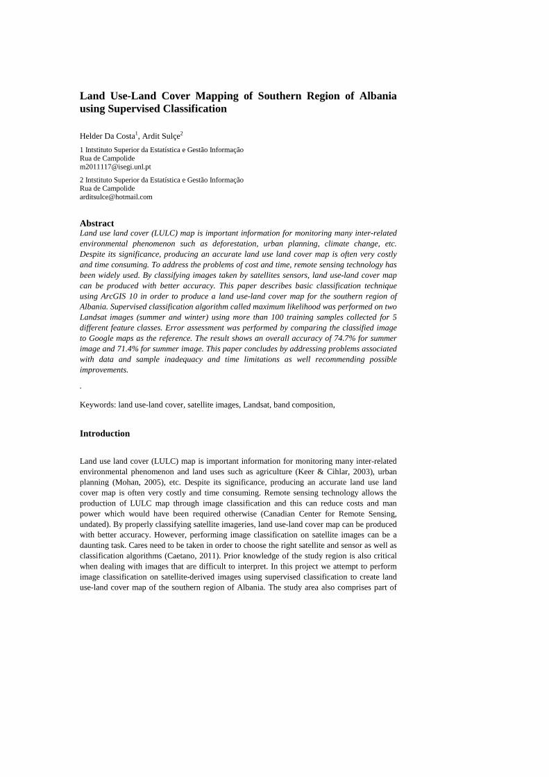
Our study region extends between 41°02’50” and 39°35’06” latitudes, and between 10°09’22” and 21°18’27” longitudes. It consists of a 160 km x 180 km area covering most of the southern part of Albania, a region characterized by hills and mountains with elevation as high as 1400m.

Figure 1. Map of Albania and the study area extent.

Materials and Methods The study is based on the secondary data, the Landsat TM5 and Landsat 7 ETM+ imageries, downloaded from Earth Explorer website (www.earthexplorer.usgs.gov), with orbit point (path 185 and 186, row 31 and 32). Since vegetation is one of the major features in land cover map, we also intended to classify a winter image and compare it to the summer image. However, the lack of better quality images made it difficult for us to find images from the same year with cloud cover less than 10%. As a consequence, we had to download Landsat TM5 for July 2009 (summer image) and Landsat 7 ETM+ image for November 2002 (winter image). These images were already been corrected radiometrically and geometrically, and thus, it was only necessary to mosaic them into a single image. For our reference map, Google Earth imageries were used. The image classification software used for this project is ArcGIS 10.

Data Exploitation After organizing all the required dataset, we started the classification process by making a true color composite of the satellite image. A visual analysis of the study region revealed that the image had a small percentage of cloud cover which we believe will affect the classification result to some extent. Due to the size of the region, it is also difficult to identidifferentiate urban cities. The major land cover types easily identified are water bodies, vegetation and soil. Another problem is that the images were taken on different time and so the level of atmospheric influences was different on both images ashown in Figure 2 by the line. We tried color correction in ArcGIS to minimize the problem but the result was not satisfying. Hence, we had to deal with it.

Figure 2. True color composite RGB 321.

In order to aid visual interpretation, visual appearance of the objects in the image was improved by image enhancement enhancement procedure is shown in can almost be differentiated by the green and yellowish colors, the soil and bare rock appear pink and very bright. The urban is shown in magenta, however, it can also be confused with soil as well.

Figure 3. Different band compositions: True colo432 (center), and RGB 542 (right).

After organizing all the required dataset, we started the classification process by making a true of the satellite image. A visual analysis of the study region revealed that the

image had a small percentage of cloud cover which we believe will affect the classification Due to the size of the region, it is also difficult to identify and

differentiate urban cities. The major land cover types easily identified are water bodies, Another problem is that the images were taken on different time and so the

level of atmospheric influences was different on both images and the difference is clearly by the line. We tried color correction in ArcGIS to minimize the problem

but the result was not satisfying. Hence, we had to deal with it.

Figure 2. True color composite RGB 321.

In order to aid visual interpretation, visual appearance of the objects in the image was techniques such as contrast stretch. An example of an

t procedure is shown in Figure 3 (right image) where different vegetation types can almost be differentiated by the green and yellowish colors, the soil and bare rock appear pink and very bright. The urban is shown in magenta, however, it can also be confused with

Different band compositions: True color composite RGB 321 (left), false color composite RGB

After organizing all the required dataset, we started the classification process by making a true of the satellite image. A visual analysis of the study region revealed that the

image had a small percentage of cloud cover which we believe will affect the classification fy and

differentiate urban cities. The major land cover types easily identified are water bodies, Another problem is that the images were taken on different time and so the

nd the difference is clearly by the line. We tried color correction in ArcGIS to minimize the problem

In order to aid visual interpretation, visual appearance of the objects in the image was techniques such as contrast stretch. An example of an

types can almost be differentiated by the green and yellowish colors, the soil and bare rock appear pink and very bright. The urban is shown in magenta, however, it can also be confused with

r composite RGB 321 (left), false color composite RGB

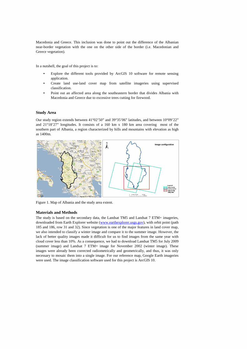
Aside from the band composition above, a Normalized Difference Vegetation Index (NDVI) was also performed as to highlight the amount of biomass on the study region. The NDVI also helps us to visualize areas where biomass is in greater amount throughout the study region.

Figure 4. Normalized Difference Vegetation Index (NDVI). The bright color from grey scale image suggest that biomass is high. On the second image with different color ramp, the healthy biomass is represented by green color.

Supervised Classification

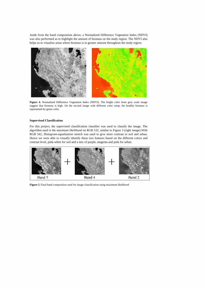
For this project, the supervised classification classifier was used to classify the image. The algorithm used is the maximum likelihood on RGB 532, similar to Figure 3 (right image).With RGB 542, Histogram-equalization stretch was used to give more contrast to soil and urban. Hence we were able to visually identify these two features based on the different colors and contrast level, pink-white for soil and a mix of purple, magenta and pink for urban.

Figure 5. Final band composition used for image classification using maximum likelihood

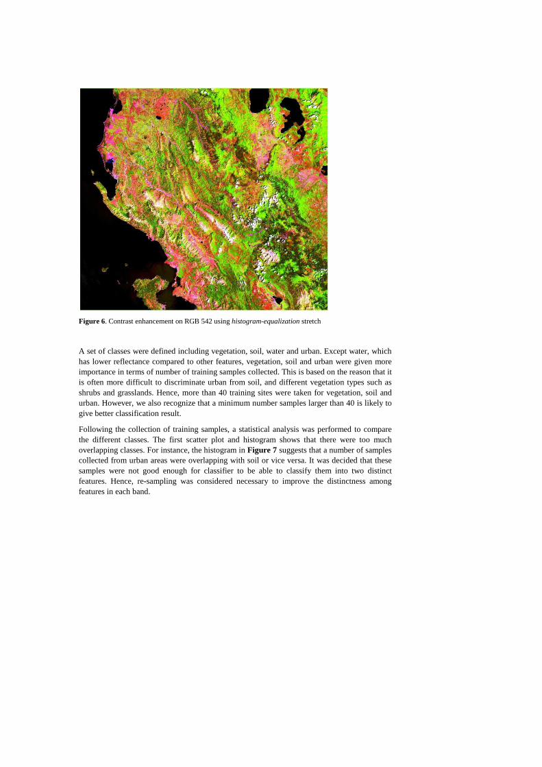
Figure 6. Contrast enhancement on RGB 542 using histogram-equalization stretch

A set of classes were defined including vegetation, soil, water and urban. Except water, which has lower reflectance compared to other features, vegetation, soil and urban were given more importance in terms of number of training samples collected. This is based on the reason that it is often more difficult to discriminate urban from soil, and different vegetation types such as shrubs and grasslands. Hence, more than 40 training sites were taken for vegetation, soil and urban. However, we also recognize that a minimum number samples larger than 40 is likely to give better classification result.

Following the collection of training samples, a statistical analysis was performed to compare the different classes. The first scatter plot and histogram shows that there were too much overlapping classes. For instance, the histogram in Figure 7 suggests that a number of samples collected from urban areas were overlapping with soil or vice versa. It was decided that these samples were not good enough for classifier to be able to classify them into two distinct features. Hence, re-sampling was considered necessary to improve the distinctness among features in each band.

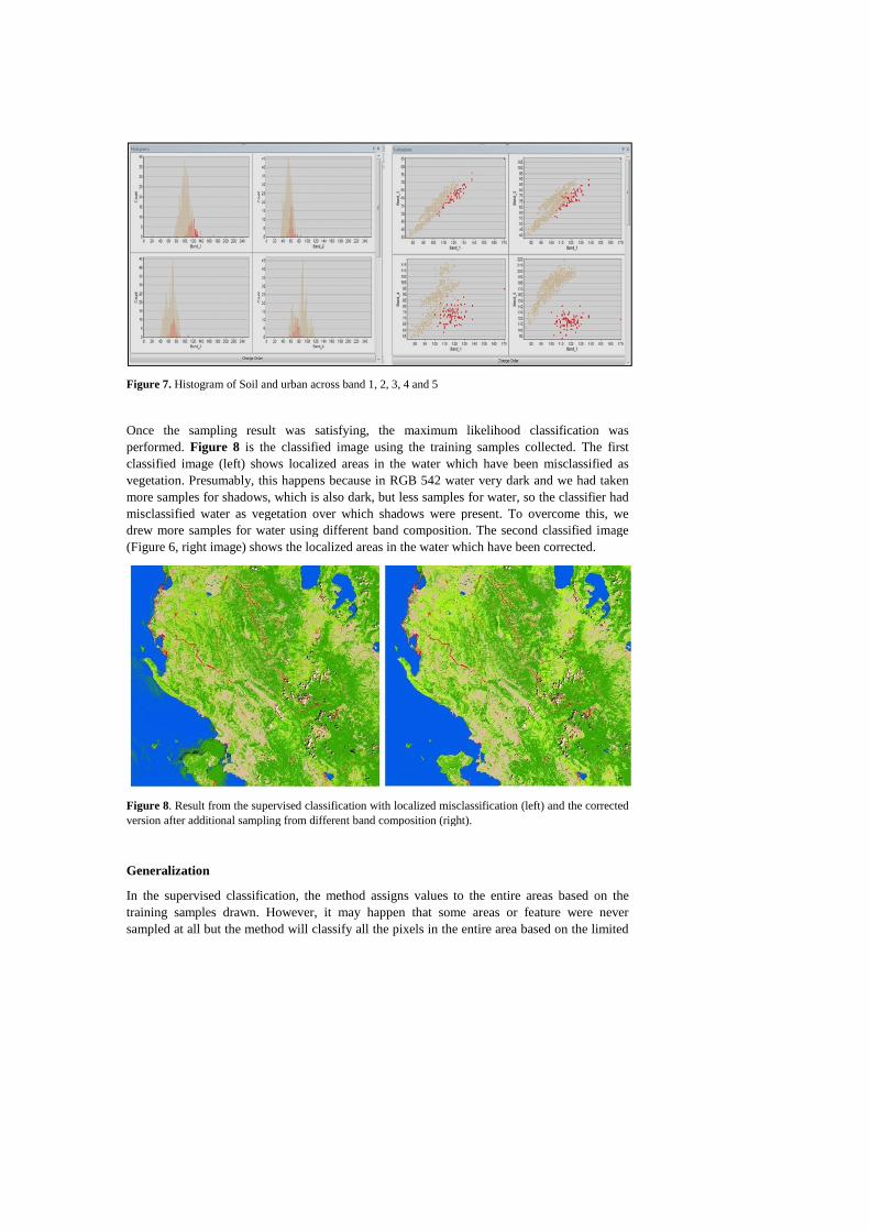
Figure 7. Histogram of Soil and urban across band 1, 2, 3, 4 and 5

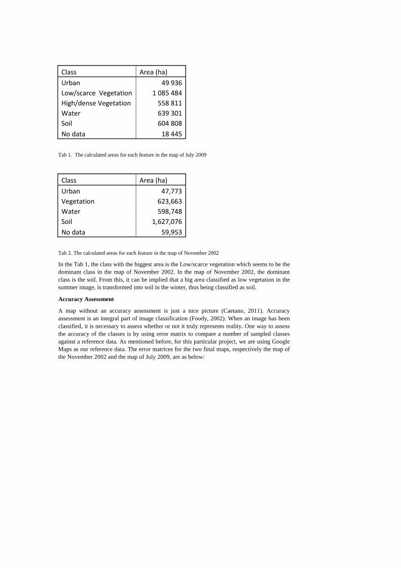
Once the sampling result was performed. Figure 8 is the classified image using the training samples collected. The first classified image (left) shows localized areas in the water which have been misclassified as vegetation. Presumably, this happens because more samples for shadows, which is also dark, but less samples for water, so the classifier had misclassified water as vegetation over which shadows were present. drew more samples for water using different band composition. The second classified image (Figure 6, right image) shows the localized areas in the water which have been corrected.

Figure 8. Result from the supervised classification with localized misclassversion after additional sampling from different band composition (right).

Generalization

In the supervised classification, the method assigns values to the entire areas based on the training samples drawn. However, it msampled at all but the method will classify all the pixels in the entire area based on the limited

Histogram of Soil and urban across band 1, 2, 3, 4 and 5

Once the sampling result was satisfying, the maximum likelihood classification was is the classified image using the training samples collected. The first

classified image (left) shows localized areas in the water which have been misclassified as ably, this happens because in RGB 542 water very dark and we had taken

more samples for shadows, which is also dark, but less samples for water, so the classifier had misclassified water as vegetation over which shadows were present. To overcome this, we rew more samples for water using different band composition. The second classified image

the localized areas in the water which have been corrected.

. Result from the supervised classification with localized misclassification (left) and the corrected version after additional sampling from different band composition (right).

In the supervised classification, the method assigns values to the entire areas based on the training samples drawn. However, it may happen that some areas or feature were never sampled at all but the method will classify all the pixels in the entire area based on the limited

cation was is the classified image using the training samples collected. The first

classified image (left) shows localized areas in the water which have been misclassified as in RGB 542 water very dark and we had taken

more samples for shadows, which is also dark, but less samples for water, so the classifier had To overcome this, we

rew more samples for water using different band composition. The second classified image

ification (left) and the corrected

In the supervised classification, the method assigns values to the entire areas based on the ay happen that some areas or feature were never

sampled at all but the method will classify all the pixels in the entire area based on the limited

training areas available. This can result in areas or pixel being classified as something different from its surrounding pixels. To minimize this discrepancy in our classified image we applied a generalization technique called majority filter. This technique reassigns pixel of an image based on the majority of contiguous neighboring pixels (ArcGIS 10 Desktop Help). It tries to eliminate small areas which are irrelevant to the analysis. We also applied boundary cleaning to smooth out the boundary between zones. Finally, we perform reclassification to make the values for each class permanent. The resulting image after filtering, boundary cleaning and reclassification is shown in Figure 9.

Figure 9. Result of Maximum Likelihood Classification with six classes

Result and Discussion

Visually comparing the classified map with the composite image from which the samples were drawn shows that urban areas were in places classified as soil/sand along the river. Eliminating the problem with extra soil training samples did not solve the problem—too many misinterpreted pixels. However, our classified image brings up two things: the loss of trees near the borderline and the type of agriculture that exist on the northeast of our study region. Firstly, we believe that the classified image had confirmed the loss of vegetation along the southeastern border of Albania. As shown in Figure 10, the presence of dense vegetation which is naturally continuous throughout the borders has a sudden break along the southeastern borderline. On this particular area, vegetation on the neighboring country, Greece, appear darker, while on the opposite of the border it is shown as shrubs/agriculture.

Figure 10. Summer image with less vegetated area near the southern border (left). Google Earth image showing less vegetated area in Albania and densely vegetated area on the opposite border.

Secondly, many pixels/area on the northeast of Albania have been classified as agriculture as well (green to brown), but we are not sure of its type. Hence, we decided to perform another supervised classification on winter image from Landsat ETM+ which was collected on November 2002. We then compared the resulting classified winter image (Figure 11) to summer image (Figure 9) and noticed the difference in vegetation but still hard to tell whether or not the particular area in question was used for irrigated or non-irrigated agriculture.

Figure 11. Result of maximum likelihood classification on winter image with five classes

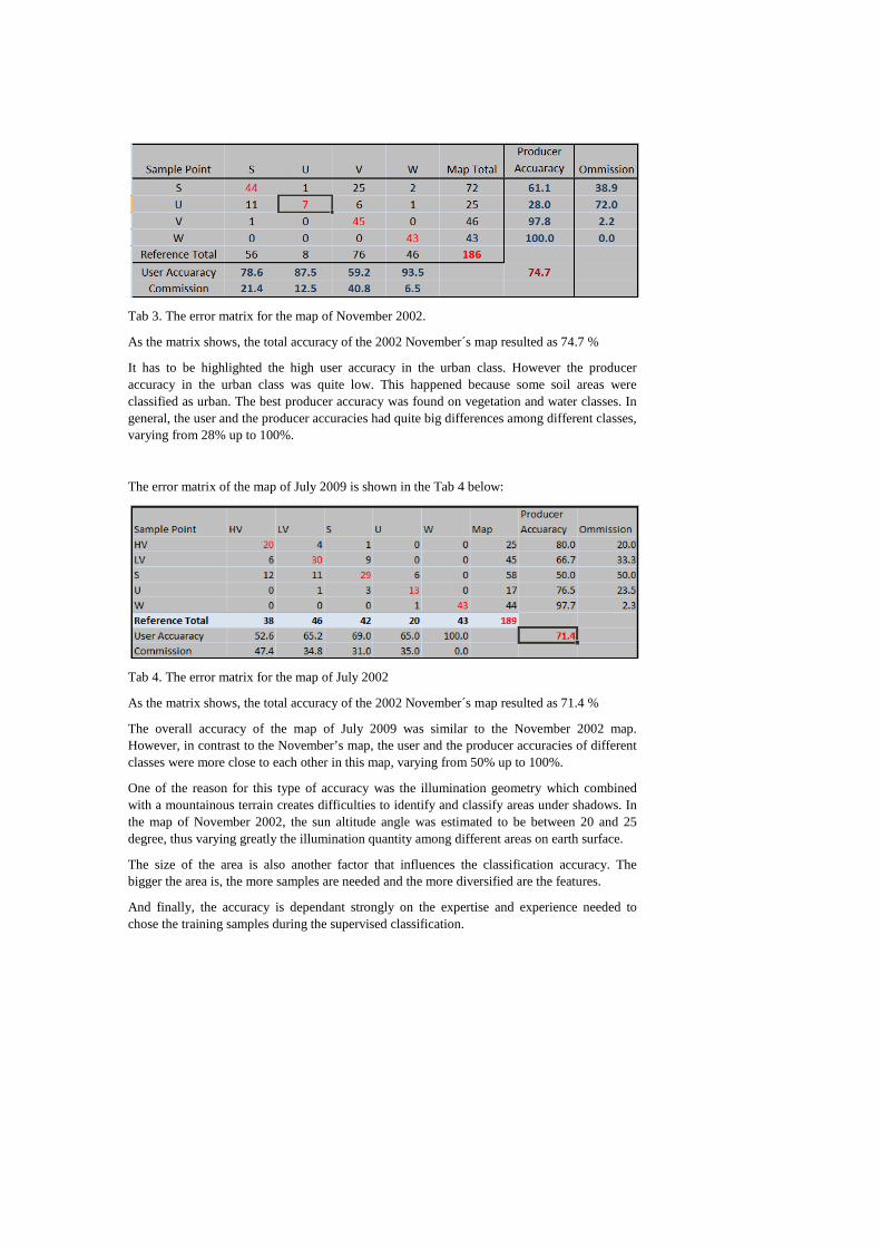
After the classified maps were produced, the areas of each class for each of the maps were calculated. The tables below give the area for each class.

Class Area (ha)

Urban 49 936

Low/scarce Vegetation 1 085 484

High/dense Vegetation 558 811

Water 639 301

Soil 604 808

No data 18 445

Tab 1. The calculated areas for each feature in the map of July 2009

Class Area (ha)

Urban 47,773

Vegetation 623,663

Water 598,748

Soil 1,627,076

No data 59,953

Tab 2. The calculated areas for each feature in the map of November 2002

In the Tab 1, the class with the biggest area is the Low/scarce vegetation which seems to be the dominant class in the map of November 2002. In the map of November 2002, the dominant class is the soil. From this, it can be implied that a big area classified as low vegetation in the summer image, is transformed into soil in the winter, thus being classified as soil.

Accuracy Assessment

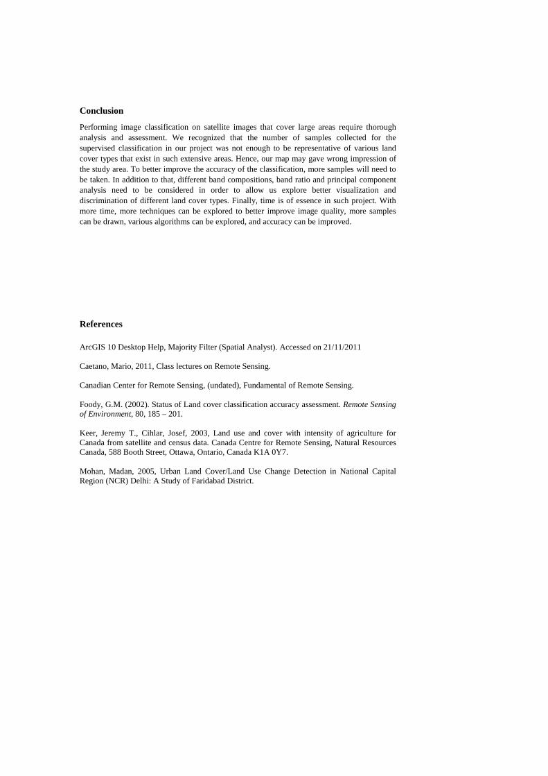
A map without an accuracy assessment is just a nice picture (Caetano, 2011). Accuracy assessment is an integral part of image classification (Foody, 2002). When an image has been classified, it is necessary to assess whether or not it truly represents reality. One way to assess the accuracy of the classes is by using error matrix to compare a number of sampled classes against a reference data. As mentioned before, for this particular project, we are using Google Maps as our reference data. The error matrices for the two final maps, respectively the map of the November 2002 and the map of July 2009, are as below:

Tab 3. The error matrix for the map of November 2002.

As the matrix shows, the total accuracy of the 2002 November´s map resulted as 74.7 %

It has to be highlighted the high user accuracy in the urban class. However the producer accuracy in the urban class was quite low. This happened because some soil areas were classified as urban. The best producer accuracy was found on vegetation and water classes. In general, the user and the producer accuracies had quite big differences among different classes, varying from 28% up to 100%.

The error matrix of the map of July 2009 is shown in the Tab 4 below:

Tab 4. The error matrix for the map of July 2002

As the matrix shows, the total accuracy of the 2002 November´s map resulted as 71.4 %

The overall accuracy of the map of July 2009 was similar to the November 2002 map. However, in contrast to the November’s map, the user and the producer accuracies of different classes were more close to each other in this map, varying from 50% up to 100%.

One of the reason for this type of accuracy was the illumination geometry which combined with a mountainous terrain creates difficulties to identify and classify areas under shadows. In the map of November 2002, the sun altitude angle was estimated to be between 20 and 25 degree, thus varying greatly the illumination quantity among different areas on earth surface.

The size of the area is also another factor that influences the classification accuracy. The bigger the area is, the more samples are needed and the more diversified are the features.

And finally, the accuracy is dependant strongly on the expertise and experience needed to chose the training samples during the supervised classification.

Conclusion

Performing image classification on satellite images that cover large areas require thorough analysis and assessment. We recognized that the number of samples collected for the supervised classification in our project was not enough to be representative of various land cover types that exist in such extensive areas. Hence, our map may gave wrong impression of the study area. To better improve the accuracy of the classification, more samples will need to be taken. In addition to that, different band compositions, band ratio and principal component analysis need to be considered in order to allow us explore better visualization and discrimination of different land cover types. Finally, time is of essence in such project. With more time, more techniques can be explored to better improve image quality, more samples can be drawn, various algorithms can be explored, and accuracy can be improved.

References

ArcGIS 10 Desktop Help, Majority Filter (Spatial Analyst). Accessed on 21/11/2011 Caetano, Mario, 2011, Class lectures on Remote Sensing. Canadian Center for Remote Sensing, (undated), Fundamental of Remote Sensing. Foody, G.M. (2002). Status of Land cover classification accuracy assessment. Remote Sensing of Environment, 80, 185 – 201. Keer, Jeremy T., Cihlar, Josef, 2003, Land use and cover with intensity of agriculture for Canada from satellite and census data. Canada Centre for Remote Sensing, Natural Resources Canada, 588 Booth Street, Ottawa, Ontario, Canada K1A 0Y7. Mohan, Madan, 2005, Urban Land Cover/Land Use Change Detection in National Capital Region (NCR) Delhi: A Study of Faridabad District.