Supervised Machine Learning Methods for Complex Data

Supervised Machine Learning Methods for Complex

Data

by

Alessio Petrozziello

School of Computing

University of Portsmouth, UK

The thesis is submitted in partial fulfilment of the requirements for the award

of the degree of Doctor of Philosophy of the University of Portsmouth

August, 2019

1

Copyright

Copyright © 2019 Alessio Petrozziello. All rights reserved.

The copyright of this thesis rests with the Author. Copies (by any means) either

in full, or of extracts, may not be made without prior written consent from the

Author.

2

Declaration

The work presented in this thesis has been carried out in the School of Comput-

ing at the University of Portsmouth under the supervision of Dr. Ivan Jordanov.

Whilst registered as a candidate for the above degree, I have not been registered

for any other research award. The results and conclusions embodied in this the-

sis are the work of the named candidate and have not been submitted for any

other academic award.

Wednesday 7th August, 2019,

Portsmouth,

Alessio Petrozziello

3

Abstract

This dissertation investigates state-of-the-art machine learning methods (both

shallow and deep) and their application for knowledge extraction, prediction,

recognition, and classification of large-scale real-world problems in different ar-

eas (healthcare, online recommender systems, pattern recognition and security,

prediction in finance, etc.).

The first part of this work focuses on the missing data problem and its impact

on a variety of machine learning tasks (i.e., classification, regression and learn

to rank), introducing new methods to tackle this problem for medium, large

and big datasets. After an initial overview of the literature on missing data

imputation, a classification task for the identification of radar signal emitters

with a high percentage of missing values in its features is investigated. Suc-

cessively, the impact of missing data on Recommender Systems is examined,

focussing on Online Travel Agencies and the ranking of their properties. In re-

lation to the missing data imputation problem, two novel approaches have been

introduced, the first one is an aggregation model of the most suitable imputa-

tion techniques based on their performance for each individual feature of the

dataset. The second one aims to impute missing values at scale (large datasets)

through a distributed neural network implemented in Apache Spark.

The second part of this dissertation investigates the use of Deep Learning tech-

niques to tackle three real-world problems. In the first one, both Convolutional

Neural Networks and Long Short Term Memory Networks are used for the

detection of hypoxia during childbirth. Next, the profitability of Multivariate

Long Short Term Memory Networks for the forecast of stock market volatility

is explored. Lastly, Convolutional Neural Networks and Stacked Autoencoders

are used to detect threats from hand-luggage and courier parcel x-ray images.

4

Contents

1 Introduction 18

1.1 Motivation . . . . . . . . . . . . . . . . . . . . . . . . . . . . . . . . 18

1.2 Original Contribution to Knowledge . . . . . . . . . . . . . . . . . 18

1.3 List of Publications . . . . . . . . . . . . . . . . . . . . . . . . . . . 20

1.3.1 Within the scope of the thesis . . . . . . . . . . . . . . . . . 20

1.3.2 Outside the scope of the thesis . . . . . . . . . . . . . . . . 22

1.4 Outline . . . . . . . . . . . . . . . . . . . . . . . . . . . . . . . . . . 22

2 Background 24

2.1 Missing Data Techniques . . . . . . . . . . . . . . . . . . . . . . . . 24

2.2 Recommender Systems . . . . . . . . . . . . . . . . . . . . . . . . . 33

2.3 Big Data Frameworks . . . . . . . . . . . . . . . . . . . . . . . . . . 36

2.3.1 Apache Hadoop . . . . . . . . . . . . . . . . . . . . . . . . 38

2.3.2 Apache Spark . . . . . . . . . . . . . . . . . . . . . . . . . . 40

2.3.3 Mention to other big data frameworks . . . . . . . . . . . . 41

2.4 Deep Neural Networks . . . . . . . . . . . . . . . . . . . . . . . . . 43

2.4.1 Convolutional Neural Networks . . . . . . . . . . . . . . . 46

2.4.2 Autoencoders . . . . . . . . . . . . . . . . . . . . . . . . . . 46

2.4.3 Long Short Term Memory Networks . . . . . . . . . . . . . 47

2.5 Evaluation Criteria . . . . . . . . . . . . . . . . . . . . . . . . . . . 49

2.5.1 Assessment of classification performance . . . . . . . . . . 50

2.5.2 Assessment of regression performance . . . . . . . . . . . 52

2.5.3 Assessment of learn to rank tasks performance . . . . . . . 54

2.5.4 Baseline sanity check . . . . . . . . . . . . . . . . . . . . . . 54

5

2.5.5 Statistical significance tests . . . . . . . . . . . . . . . . . . 56

2.5.6 Time as a performance measure . . . . . . . . . . . . . . . 57

2.6 Conclusion . . . . . . . . . . . . . . . . . . . . . . . . . . . . . . . . 60

3 Missing Data Imputation 61

3.1 Literature Review . . . . . . . . . . . . . . . . . . . . . . . . . . . . 61

3.2 Radar Signal Recognition with Missing Data . . . . . . . . . . . . 65

3.2.1 Background . . . . . . . . . . . . . . . . . . . . . . . . . . . 65

3.2.2 Data pre-processing . . . . . . . . . . . . . . . . . . . . . . 67

3.2.3 Supervised radar classification techniques . . . . . . . . . 70

3.2.4 Assessment baseline . . . . . . . . . . . . . . . . . . . . . . 72

3.2.5 Classification results . . . . . . . . . . . . . . . . . . . . . . 75

3.2.6 Discussion . . . . . . . . . . . . . . . . . . . . . . . . . . . . 83

3.3 Scattered Feature Guided Data Imputation . . . . . . . . . . . . . 84

3.3.1 Proposed method . . . . . . . . . . . . . . . . . . . . . . . . 84

3.3.2 Empirical study design . . . . . . . . . . . . . . . . . . . . 86

3.3.3 Results . . . . . . . . . . . . . . . . . . . . . . . . . . . . . . 88

3.3.4 Discussion . . . . . . . . . . . . . . . . . . . . . . . . . . . . 97

3.4 Online Traveling Recommender System with Missing Values . . . 99

3.4.1 Data pre-processing and feature engineering . . . . . . . . 100

3.4.2 Exploratory analysis . . . . . . . . . . . . . . . . . . . . . . 104


3.4.4 Results . . . . . . . . . . . . . . . . . . . . . . . . . . . . . . 111

3.4.5 Discussion . . . . . . . . . . . . . . . . . . . . . . . . . . . . 119

3.5 Large Scale Missing Data Imputation . . . . . . . . . . . . . . . . . 120

3.5.1 A distributed Neural Network architecture on Spark . . . 121

6


3.5.3 Results and discussion . . . . . . . . . . . . . . . . . . . . . 125

3.6 Conclusion . . . . . . . . . . . . . . . . . . . . . . . . . . . . . . . . 129

4 Deep Learning Methods for Real-World Problems 130

4.1 Deep Learning for fetal monitoring in labour . . . . . . . . . . . . 130

4.1.1 Datasets . . . . . . . . . . . . . . . . . . . . . . . . . . . . . 133

4.1.2 Proposed Deep Learning models . . . . . . . . . . . . . . . 136

4.1.3 State of the art methods . . . . . . . . . . . . . . . . . . . . 139

4.1.4 Performance metrics . . . . . . . . . . . . . . . . . . . . . . 140

4.1.5 Results . . . . . . . . . . . . . . . . . . . . . . . . . . . . . . 141

4.1.6 Discussion . . . . . . . . . . . . . . . . . . . . . . . . . . . . 149

4.2 Deep Learning for stock market volatility forecasting . . . . . . . 152

4.2.1 Data . . . . . . . . . . . . . . . . . . . . . . . . . . . . . . . 155

4.2.2 Experimental setup . . . . . . . . . . . . . . . . . . . . . . . 156

4.2.3 Compared methods . . . . . . . . . . . . . . . . . . . . . . 159

4.2.4 Results and discussion . . . . . . . . . . . . . . . . . . . . . 163

4.3 Deep Learning for threat detection in luggage from x-ray images 174

4.3.1 Related Work . . . . . . . . . . . . . . . . . . . . . . . . . . 175

4.3.2 Dataset . . . . . . . . . . . . . . . . . . . . . . . . . . . . . . 176

4.3.3 Threat identification framework . . . . . . . . . . . . . . . 177

4.3.4 Experimentation and Results . . . . . . . . . . . . . . . . . 178

4.4 Conclusion . . . . . . . . . . . . . . . . . . . . . . . . . . . . . . . . 182

5 Conclusion 183

5.1 Missing data Imputation . . . . . . . . . . . . . . . . . . . . . . . . 183

5.2 Deep Learning Methods for Real-World Problems . . . . . . . . . 184

7

5.3 Further Research Directions . . . . . . . . . . . . . . . . . . . . . . 186

A

Scattered Feature Guided Data Imputation 204

B

Online Traveling Recommender System with Missing Values 211

C

Deep Learning for fetal monitoring in labour 212

D

Deep Learning for stock market volatility forecasting 213

E

Deep Learning for threat detection in luggage from x-ray images 214

8

List of Tables

2.1 Data processing engines for Hadoop. . . . . . . . . . . . . . . . . . 43

2.2 Confusion matrix for a binary problem. . . . . . . . . . . . . . . . 50

3.1 Sample radar data subset. . . . . . . . . . . . . . . . . . . . . . . . 66

3.2 Sample radar subset with imputed continuous values. . . . . . . . 67

3.3 Data description and percentage of missing values. . . . . . . . . 68

3.4 Sample subset with imputed radar data and natural number cod-

ing of RFC, PRC, PDC, and ST. . . . . . . . . . . . . . . . . . . . . 69

3.5 Example of binary coding for 32-level categorical variable. . . . . 69

3.6 Example of dummy coding for 32-level categorical variable. . . . 70

3.7 Classifiers Inner Accuracy (IA) and Outer Accuracy (OA) com-

pared to the best Overall Classifier Accuracy (OCA) in the 11

class classification. . . . . . . . . . . . . . . . . . . . . . . . . . . . 82

3.8 Scattered Feature Guided Data Imputation example. . . . . . . . . 86

3.9 Datasets used in the empirical study. The last three columns

show the number and type of attributes (R - Real, I - Integer, C -

Categorical). . . . . . . . . . . . . . . . . . . . . . . . . . . . . . . . 87

3.10 Hyper-parameters setting. . . . . . . . . . . . . . . . . . . . . . . . 89

3.11 Standardized Accuracy (SA) values achieved by sFGDI, the base-

line (median imputation) and state-of-the-art (KNNI, BTI, MICE,

and bPCA) techniques over the 13 datasets for 5-fold cross vali-

dation with 25% MCAR. . . . . . . . . . . . . . . . . . . . . . . . . 89

3.12 RMSE (MAE) significance test for 5-fold cross validation with

25% (a) and 50% (b) MCAR in the test set. . . . . . . . . . . . . . . 91

3.13 RE* metric of sFGDI and four state-of-the-art imputation meth-

ods for the 13 datasets for 5-fold cross validation with 25% MCAR. 92

9

3.14 RMSE (MAE) significance test for 30-fold cross validation with:

(a) 25%; and (b) 50% MCAR in the test set. . . . . . . . . . . . . . . 93




dation with 25% MAR. . . . . . . . . . . . . . . . . . . . . . . . . . 95




dation with 25% MNAR. . . . . . . . . . . . . . . . . . . . . . . . . 95

3.17 RMSE (MAE) significance test for 5-fold cross validation with

25% MAR (a) and 25% MNAR (b) in the test set. . . . . . . . . . . 96

3.18 Amenities Table . . . . . . . . . . . . . . . . . . . . . . . . . . . . . 102

3.19 Description of the aggregated dimensions from the cleansed click-

stream dataset. . . . . . . . . . . . . . . . . . . . . . . . . . . . . . . 103

3.20 Description of the aggregated segments from the cleansed click-

stream dataset. . . . . . . . . . . . . . . . . . . . . . . . . . . . . . . 103

3.21 Cleansed and aggregated amenities for each property. . . . . . . . 104

3.22 Cleansed and cross-joined table between active properties and des-

tinations. . . . . . . . . . . . . . . . . . . . . . . . . . . . . . . . . . 104

3.23 List of property types. . . . . . . . . . . . . . . . . . . . . . . . . . 105

3.24 Spearman Correlation between Impressions, Clicks, Bookings, Rank,

Guest Rating and Star Rating. . . . . . . . . . . . . . . . . . . . . . . 106

3.25 Example of a search where no VR are displayed in the top 10

positions (head of the list). . . . . . . . . . . . . . . . . . . . . . . . 109

3.26 MAP@5 accuracy scored by the three proposed similarity mea-

sures. . . . . . . . . . . . . . . . . . . . . . . . . . . . . . . . . . . . 114

3.27 Guest rating and star rating imputation errors. . . . . . . . . . . . 116

10

3.28 Offline experimentation on one month of real world searches. . . 117

3.29 Neural Network Trait. . . . . . . . . . . . . . . . . . . . . . . . . . 122

3.30 Example of network specification for D-NNI. . . . . . . . . . . . . 123

3.31 Example of Missing Imputation Stage in a Spark pipeline. . . . . 123

3.32 Sample of the dataset containing the features used for the prop-

erties recommendation. . . . . . . . . . . . . . . . . . . . . . . . . . 124

3.33 Summary of the features used in the OTAs dataset. . . . . . . . . 124

3.34 Average and std run time (in minutes) over 10 runs. . . . . . . . . 127

3.35 Speedup ratio of the NN compared to the sequential model. . . . 127

4.1 Selected training and testing results for the two neural networks

models. . . . . . . . . . . . . . . . . . . . . . . . . . . . . . . . . . . 142

4.2 Comparison of the proposed models (median of 5 runs) on Test

Set A (n=4429). . . . . . . . . . . . . . . . . . . . . . . . . . . . . . 144

4.3 Quality groups on Test Set A. . . . . . . . . . . . . . . . . . . . . . 147

4.4 Testing on the SPaM17 dataset. . . . . . . . . . . . . . . . . . . . . 148

4.5 Testing on the CTU-UHB dataset. . . . . . . . . . . . . . . . . . . . 148

4.6 Dow Jones Industrial Average assets used as case study. . . . . . . 156

4.7 NASDAQ 100 assets used as case study. . . . . . . . . . . . . . . . 157

4.8 Hyper-parameters for the LSTM. The optimal value of each hyper-

parameter has been selected through a grid search on the defined

range. . . . . . . . . . . . . . . . . . . . . . . . . . . . . . . . . . . . 158

4.9 Evaluation Metrics for the DJI 500 dataset. . . . . . . . . . . . . . . 163

4.10 Debold-Mariano statistic for the DJI 500 dataset for the LSTM-29. 166

4.11 Average with Std (in brackets) errors, Median with MAD (in brack-

ets) errors for the four models at different volatility regimes on

the DJI 500 dataset. . . . . . . . . . . . . . . . . . . . . . . . . . . . 167

11

4.12 Debold-Mariano statistic for the DJI 500 dataset (with a p-value

given in brackets) for the LSTM-29 against LSTM-1, R-GARCH

and GJR-MEM for the four volatility regimes. . . . . . . . . . . . . 167

4.13 MSE before and during the crisis on the DJI 500 dataset for the

four models. . . . . . . . . . . . . . . . . . . . . . . . . . . . . . . . 169



the NASDAQ 100 dataset. . . . . . . . . . . . . . . . . . . . . . . . 173

4.15 Debold-Mariano statistic for the NASDAQ 100 dataset (with a

p-value given in brackets) for the LSTM-1 . . . . . . . . . . . . . . 173



the DJI 500 and NASDAQ 100 datasets. . . . . . . . . . . . . . . . 174

4.17 Baggage dataset results. . . . . . . . . . . . . . . . . . . . . . . . . 180

4.18 Parcel dataset results. . . . . . . . . . . . . . . . . . . . . . . . . . . 181

D.1 Evaluation Metrics for the NASDAQ 100 dataset: The MSE, QLIKE

and Pearson measures are reported for each asset and for each

compared model. . . . . . . . . . . . . . . . . . . . . . . . . . . . . 213

12

List of Figures

2.1 Missing data methodologies taxonomy. . . . . . . . . . . . . . . . 25

2.2 Processing engine flow charts. . . . . . . . . . . . . . . . . . . . . . 37

2.3 Topological differences between a DLA network and ELM net-

work. . . . . . . . . . . . . . . . . . . . . . . . . . . . . . . . . . . . 44

2.4 LSTM architecture. . . . . . . . . . . . . . . . . . . . . . . . . . . . 48

2.5 An example of speedup analysis. . . . . . . . . . . . . . . . . . . . 59

2.6 An example of size-up analysis. . . . . . . . . . . . . . . . . . . . . 60

3.1 Label imputation for MI, BTI and KNNI over 30 runs for 2 classes. 73

3.2 Label imputation for MI, BTI and KNNI over 30 runs for 11 classes. 74

3.3 Root mean square error (RMSE) for the imputation of the contin-

uous values (30 runs). . . . . . . . . . . . . . . . . . . . . . . . . . 75

3.4 Density function for the features: RFmi, PRImi, PDmi, SPmi on

the dataset without missing value. . . . . . . . . . . . . . . . . . . 76

3.5 Confusion matrix and ROC Curve illustrating the RF classifica-

tion results for the two classes, after using BTI with continuous

value coding (Military and Civil). . . . . . . . . . . . . . . . . . . . 77

3.6 Confusion matrix illustrating the RF classification results for the

11 classes, after using BTI with continuous value coding. . . . . . 78

3.7 Classification performance results of the classifiers (RF, NN and

SVM) in the case of 2 classes after using three different impu-

tation techniques (BTI, KNNI and MI), for the three different

groups of coding (binary, continuous and dummy). . . . . . . . . 79

3.8 Classification performance results of the classifiers (RF, NN and

SVM) in the case of 11 classes after using three different impu-

tation techniques (BTI, KNNI and MI), for the three different

groups of coding (binary, continuous and dummy). . . . . . . . . 80

13

3.9 Cumulative error bar plot of the four considered imputation meth-

ods for the Red Wine dataset. . . . . . . . . . . . . . . . . . . . . . 90

3.10 Training time in seconds of the five considered imputation meth-

ods over the 13 datasets. . . . . . . . . . . . . . . . . . . . . . . . . 97

3.11 Density plot showing for each property type, the density of prop-

erties in each rank. . . . . . . . . . . . . . . . . . . . . . . . . . . . 107

3.12 Distribution of guest rating and star rating. . . . . . . . . . . . . . 108

3.13 Pareto front example for one search. . . . . . . . . . . . . . . . . . 111

3.14 Workflow for a machine learning pipeline on ML-Spark. . . . . . 112

3.15 All Pareto front solutions standardized with 0-mean and unit-

variance. . . . . . . . . . . . . . . . . . . . . . . . . . . . . . . . . . 118

3.16 Distributed Neural Network architecture in Spark. . . . . . . . . . 121

3.17 Log growth of the properties in the catalogue and log growth of

missing data. . . . . . . . . . . . . . . . . . . . . . . . . . . . . . . . 125

3.18 Boxplot for the R2 measure on the 57 imputed variables. . . . . . . 126

3.19 Boxplot for the R2 measure on the 57 imputed variables. . . . . . . 127

3.20 Predicted and observed values for the D-NNI. . . . . . . . . . . . 128

4.1 Cardiotocogram (CTG) in labour (a 30min snippet). . . . . . . . . 131

4.2 Convolutional Neural Network topology. . . . . . . . . . . . . . . 137

4.3 Long Short Term Memory Network topology. . . . . . . . . . . . . 137

4.4 Multimodal Convolutional Neural Network topology. . . . . . . . 138

4.5 Stacked MCNN topology for 1st and 2nd stage classification. . . . 139

4.6 Optimization contour plot. . . . . . . . . . . . . . . . . . . . . . . . 142

4.7 Left: Comparison of the two Deep Learning models, OxSys 1.5

and Clinical practice o the test set (x2 test for comparison of pro-

portions); Right: ROC curves CNN vs LSTM models (Oxford test

set: 5314 cases). . . . . . . . . . . . . . . . . . . . . . . . . . . . . . 143

14

4.8 Robustness of CNN with respect to the size of training dataset

over 30 runs (FPR is fixed at 15%). . . . . . . . . . . . . . . . . . . 143

4.9 Performance on last 60min of CTG. . . . . . . . . . . . . . . . . . . 144

4.10 ROC curves for the four quality groups (Testing Set A, n = 4429). 147

4.11 The proposed model for DJI 500 is a stack of two LSTM with 58

and 29 neurons each and a dense activation layer on the top. The

size of the dense layer is one in the univariate approach (LSTM-1)

and 29 in the multivariate one (LSTM-29). . . . . . . . . . . . . . . 157

4.12 LSTM-29 one step ahead predictions for all assets of the DJI 500

dataset (excluded the index fund SPY). . . . . . . . . . . . . . . . . 164

4.13 Relationship between difference in MSE and variance of volatility. 165

4.14 Cumulative MSE for the four models at different volatility regimes

(VL, L, H, and VH). The four volatility levels are calculated using

the percentiles at 50, 75 and 95 over the 29 assets. The different

scale on the y-axis is due to the magnitude of the error in the four

volatility regimes. . . . . . . . . . . . . . . . . . . . . . . . . . . . . 168

4.15 Relationship between MSE ratios pre-crisis and in-crisis. . . . . . 170

4.16 Cumulative MSE for the four models at different volatility regimes

(VL, L, H, and VH). The four volatility levels are calculated using

the percentiles at 50, 75 and 95 over the 92 assets. The different

scale on the y-axis is due to the magnitude of the error in the four

volatility regimes. . . . . . . . . . . . . . . . . . . . . . . . . . . . . 172

4.17 Cumulative MSE for the LSTM and RNN methods (both univari-

ate and multivariate). . . . . . . . . . . . . . . . . . . . . . . . . . . 174

4.18 Baggage pre-processing image sample . . . . . . . . . . . . . . . . 177

4.19 Parcel pre-processing image sample . . . . . . . . . . . . . . . . . 179

B.1 Code snippet for cluster similarity prediction based on geograph-

ical features. . . . . . . . . . . . . . . . . . . . . . . . . . . . . . . . 211

15

B.2 Code snippet for Jaccard and weighted hamming similarity mea-

sures in scala. . . . . . . . . . . . . . . . . . . . . . . . . . . . . . . 211

C.1 Convolutional Neural Network python definition for FHR. . . . . 212

D.1 LSTM-92 one step ahead predictions for the NASDAQ 100 dataset

(APPL to EA assets). The observed time series are given in gray

and the predicted volatility values in black. . . . . . . . . . . . . . 215


(EBAY to MXIM assets). The observed time series are given in

gray and the predicted volatility values in black. . . . . . . . . . . 216


(MYL to XRAY assets). The observed time series are given in gray

and the predicted volatility values in black. . . . . . . . . . . . . . 217

E.1 Weights learned from the first autoencoder for threats and be-

nign detection. . . . . . . . . . . . . . . . . . . . . . . . . . . . . . . 218

E.2 Autoencoder topology. . . . . . . . . . . . . . . . . . . . . . . . . . 218

16

Glossary

Abbreviation MeaningMAR Missing at randomMCAR Missing completely at randomMNAR Missing not at randomMI Multiple ImputationMICE Multiple Imputation Chained EquationsBTI Bagged Tree ImputationKNNI K-Nearest Neighbours ImputationSVDI Single Value Decomposition ImputationbPCA Bayesian Principal Component AnalysisEM Expectation MaximizationRFI Random Forests ImputationBGTI Gradient Boosted Trees ImputationLRI Linear Regression ImputationRS Recommender SystemsCF Collaborative FilteringCBF Content-Based FilteringHDFS Hadoop Distributed File SystemRDD Resilient Distributed DatasetsML Machine LearningELM Extreme Learning MachineDLA Deep Learning ApproachNN Neural NetworksRBM Restricted Boltzmann MachinesCNN Convolutional Neural NetworksLSTM Long Short Term Memory NetworksRNN Recurrent Neural NetworkROC Receiver Operating CharacteristicTPR True Positive RateTPR False Positive RateAUC Area Under the CurveMAE Mean Absolute Error

Abbreviation MeaningMSE Mean Squared ErrorRMSE Root Mean Squared ErrorNRMSE Normalized Root Mean Squared ErrorSA Standard AccuracyRE* Variance Relative ErrorMAP@X Mean Average precision at XDM Diebold-MarianoSOM Self-Organized MapEOF Empirical Orthogonal FunctionsSVM Support Vector MachinesESM Electronic Support MeasuresRBF Radial Basis FunctionOCA Overall Classifier AccuracyOE Outer ErrorIE Inner ErrorIA Inner AccuracyOA Outer AccuracysFGDI Scattered Feature Guided Data ImputationVR Vacation RentalsSGD Stochastic Gradient DescentD-NNI Distributed Neural Network ImputationCTG CardiotocogramDC Decelerative CapacityPRSA Phase Rectified Signal AveragingMCNN Multimodal Convolutional Neural NetworksSPaM Signal Processing and Monitoring WorkshopCTU-UHB Czech Technical University / University Hospital BrnoGARCH Generalized Autoregressive Conditionally HeteroskedasticMEM Multiplicative Error ModelsR-GARCH Realized GARCHDJI 500 Dow Jones Industrial Average index

17

1 Introduction

1.1 Motivation

The term machine learning was coined in 1959 (Kohavi and Provost, 1998) and

refers to the ability of machines to learn from data. The machine learning field

slowly progressed through the years with contributions from a variety of dis-

ciplines such as statistics, optimization and data mining. However, the last 10

years have seen an extensive and quick growth in interest for the discipline,

being mainly driven by two factors: the availability of inexpensive computer

resources and the necessity to process and learn from the vast amount of data

being generated every day, and referred as the Big Data era (McAfee et al., 2012).

This amount of data collected by public entities and private companies, and

awaiting to be analysed, poses new large-scale real-world problems that chal-

lenges scientists and industries around the world. All these real-world prob-

lems have usually some commonalities: large amount of available data, miss-

ing values, high dimensional hyper-parameter spaces and strong non-linear re-

lationships of the collected variables. The research presented in this thesis is

motivated by the challenge posed into addressing and providing solutions to

large-scale real-world problems. A variety of machine learning methods are

here proposed, implemented and compared into the quest to advance the state

of the art of several challenging industrial and academic tasks. The original

contribution to knowledge for each tackled problem is described in Section 1.2,

the dissemination of the knowledge through peer reviewed articles is listed in

Section 1.3, while a detailed outline of the thesis is described in Section 1.4.

1.2 Original Contribution to Knowledge

This dissertation investigates different aspects of the missing data imputation

problem (Chapter 3) and three large-scale real-world problems tackled through

the use of Deep Learning techniques (Chapter 4). The original contribution to

knowledge can be summarised as follow:

18

• In Section 3.2 I compare three methods for dealing with large amount of

missing values in intercepted radar signal data. The imputation perfor-

mance is assessed on both binary and multi-class classification tasks for

the identification of the signal emitters. Furthermore, I introduce two new

evaluation metrics (namely Inner and Outer accuracies) to better assess

the classification performance in the multi-class setting.

• In Section 3.3 I propose a novel multivariate data imputation approach

(namely Feature Guided Data Imputation) for dealing with a variety of

missingness types. I report results from the comparison with two single

imputation techniques and four state-of-the-art multivariate methods on

several datasets from the public domain.

• In Section 3.4 I investigate the impact of missing data (cold start problem)

in a real-word learn to rank task (online travel agency properties ranking).

After an initial investigation, I show how the imputation of missing val-

ues can benefit the ranking of properties which have been recently added

to the catalogue.

• In Section 3.5 I tackle the problem of missing values imputation for big

data, proposing an original missing data technique based on Distributed

Neural Networks with Mini-batch Stochastic Gradient Descent on Spark.

The proposal is tested on a real-world recommender system dataset where

the missing data is generally a problem for new items, biasing the ranking

toward popular items. The model is compared with both univariate and

multivariate imputation techniques, and its performance validated using

prediction accuracy and computational speed.

• In Section 4.1 I investigate the use of Deep Learning models for hypoxia

detection during childbirth. Both Convolutional Neural Networks and

Long Short Term Memory Neural Networks are compared with existing

computerized approaches and current clinical practice on both private

and publicly available datasets. Furthermore, a novel Multimodal Convo-

lutional Neural Networks is proposed to accommodate inputs of different

19

types and dimensions.

• In Section 4.2 I explore the profitability of the application of Deep Learn-

ing techniques to the volatility forecasting problem. The proposed Multi-

variate Long Short Term Memory Neural Networks is quantitatively com-

pared in different market regimes with classic univariate and multivariate

Recurrent Neural Networks, and with the univariate parametric models

Realized Generalized Autoregressive Conditionally Heteroskedastic and

Multiplicative Error Models, which are widely used benchmarks in this

field.

• In Section 4.3 I use Deep Learning techniques for the automation of threat

objects detection from x-ray scans of passengers luggage and courier parcels.

The classification is performed on raw data and after a variety of pre-

processing steps. The Deep Learning methods performance are compared

on two datasets with widely used classification techniques such as shal-

low neural networks and random forests.

The above-listed contributions have been disseminated by:

• Presenting the research outcomes to six international conferences and con-

gresses;

• Preparing five journal papers, one of which has been published, and four

are under review.

1.3 List of Publications

1.3.1 Within the scope of the thesis

JOURNALS

1. A. Petrozziello, A. Serra, L. Troiano, I. Jordanov, M. La Rocca, G. Storti,

and R. Tagliaferri, Deep Learning for Volatility Forecasting, Elsevier In-

formation Sciences (under review).

20

2. A. Petrozziello, I. Jordanov, A.T. Papageorghiou, C.W.G. Redman, and A.

Georgieva, Multimodal Convolutional Networks to detect the fetus at risk

of asphyxia during labour, IEEE Access.

3. I. Jordanov, N. Petrov and A. Petrozziello, Classifiers accuracy improve-

ment based on missing data imputation, Journal of Artificial Intelligence

and Soft Computing Research (2018).

CONFERENCE PROCEEDINGS

4. A. Petrozziello and I. Jordanov, Automated Deep Learning for Threat De-

tection in Luggage from X-ray Images, Springer Special Event on Analysis

of Experimental Algorithms (SEA 2019).

5. A. Petrozziello and I. Jordanov, Feature Based Multivariate Data Impu-

tation, 4th Annual Conference on machine Learning, Optimization and

Data science (LOD 2018).

6. A. Petrozzielloa, I. Jordanov, A.T. Papageorghiou, C.W.G. Redman, and

A. Georgieva, Deep Learning for Continuous Electronic Fetal Monitoring

in Labor, IEEE 40th International Engineering in Medicine and Biology

Conference (EMBC 2018).

7. A. Petrozziello, C. Sommeregger and I. Jordanov, Distributed Neural Net-

works for Missing Big Data Imputation, IEEE International Joint Confer-

ence on Neural Networks (IJCNN 2018).

8. A. Petrozziello and I. Jordanov, Column-wise Guided Data Imputation,

17th International Conference on Computational Science (ICCS 2017).

9. A. Petrozziello and I. Jordanov Data Analytics for Online Traveling Rec-

ommendation System: A Case Study, IASTED’s 36th International Con-

ference on Modelling, Identification and Control (MIC 2017).

10. I. Jordanov, N. Petrov and A. Petrozziello, Supervised Radar Signal Classi-

fication, IEEE International Joint Conference on Neural Networks (IJCNN

2016).

21

1.3.2 Outside the scope of the thesis

JOURNALS

11. F. Sarro and A. Petrozziello, Linear Programming as a Baseline for Soft-

ware Effort Estimation, ACM Transactions on Software Engineering and

Methodology (2018).

12. A. Petrozziello, G. Cervone, P. Franzese, S.E. Haupt, R. Cerulli, Source

Reconstruction of Atmospheric Releases with Limited Meteorological Ob-

servations Using Genetic Algorithms, Applied Artificial Intelligence Jour-

nal (2017).

CONFERENCE PROCEEDINGS

13. F. Sarro, A. Petrozziello and M. Harman, Multi-Objective Effort Estima-

tion, ACM 38th International Conference on Software Engineering (ICSE

2016).

1.4 Outline

This thesis is organized in five chapters. The first chapter discusses the mo-

tivation for conducting this research (Section 1.1), including a section on the

original contribution (Section 1.2), a list of peer-reviewed publications that dis-

seminates the key research outcomes (Section 1.3) and the organization of the

thesis (Section 1.4).

Chapter 2 provides a background on the topics covered in Chapter 3 and Chap-

ter 4. Section 2.1 describes the state-of-art techniques used in missing data

imputation; Section 2.2 gives an introduction on recommender systems; Sec-

tion 2.3 overviews the most important frameworks used for big data process-

ing; Section 2.4 illustrates deep neural networks architectures; while Section 2.5

describes the most widely used evaluation criteria for classification, regression

and learn to rank tasks.

22

Chapter 3 investigates the impact of missing values on a variety of machine

learning tasks (i.e., classification, regression and learn to rank) and introduces

new methods to tackle this problem for medium, large and big datasets. Sec-

tion 3.1 overviews the literature on missing data imputation, focussing on the

state-of-art methods. Section 3.2 studies a classification problem for the identi-

fication of radar signal emitters with a high percentage of missing values in its

features. Section 3.3 proposes an aggregation model of the most suitable impu-

tation techniques based on their performance for each individual feature of the

dataset. Section 3.4 investigates the missing data and consequent long tail prob-

lem for recommender systems, while Section 3.5 introduces a novel distributed

algorithm for the imputation of missing data at scale.

Chapter 4 investigates Deep Learning techniques applied to three real-world

problems. Section 4.1 examines the use of Convolutional Neural Networks and

Long Short Term Memory Networks for monitoring fetal health during child-

birth, taking into account both contractions and fetal heart rate. Furthermore, a

novel architecture is presented, namely Multimodal Convolutional Neural Net-

work, which can handle both raw signals and additional features in one model.

Section 4.2 explores the use of a Multivariate Long Short Term Memory Net-

works for the forecast of stock market volatility. The proposed architecture is

compared with both Univariate Long Short Term Memory Networks and state-

of-the-art techniques used in the financial sector. Section 4.3 considers the use of

Convolutional Neural Networks and Stacked Autoencoders for the detection of

threats (e.g., firearm components) from x-ray scans collected during airport se-

curity clearance process and courier parcels inspection. The investigated tech-

niques are compared to shallow Neural Networks and Random Forests and

their performance are reported over a variety of image pre-processing steps,

and operational settings.

Chapter 5 concludes the thesis by summarising the contributions made in this

research work and outlines ideas for further investigation (Section 5.3).

23

2 Background

This chapter provides the background needed to better understand the research

pursued in Chapter 3 and Chapter 4.

Section 2.1 describes all the missing data imputation state-of-art techniques

used through Chapter 3, focussing on their strengths, weaknesses, and hyper-

parameters needed. Section 2.2 gives an introduction on recommender systems,

topic discussed in Section 3.4 and Section 3.5. The section covers a variety of rec-

ommender systems, highlighting their use cases and respective challenges. Sec-

tion 2.3 overviews the most important frameworks used for big data processing,

describing, for each of them, peculiarities and limitations. Section 2.4 illustrates

the three most used deep neural networks architectures: autoencoders, convo-

lutional neural networks, and long short term memory neural networks. All

vanilla implementations and new topologies are compared through Chapter 4.

Finally, Section 2.5 describes the most widely used evaluation criteria for clas-

sification, regression and learn to rank tasks. Furthermore, baseline methods

used as benchmark against new proposed techniques and statistical tests to en-

sure the statistical significance of the results are here reported.

2.1 Missing Data Techniques

Ideally, dealing with missing values requires an analysis strategy that leads to

the least biased estimation, without losing statistical power. The challenge is

the contradictory nature of those criteria: using the information contained in

partial record (keeping the statistical power), while substituting the missing

values with estimates, which inevitably brings biases. Mechanisms of miss-

ing data belong to three categories (Enders, 2010; Schmitt et al., 2015): Miss-

ing At Random (MAR), where the missingness may depend on observed data

but not on unobserved data (in other words, the cause of missingness is con-

sidered); Missing Completely At Random (MCAR), which is a special case of

MAR, where the probability that an observation is missing is unrelated to its

value or to the value of any other variable; Missing Not At Random (MNAR),

24

where the missingness depends on unobserved data. The last group usually

yields biased parameter estimates, while MCAR and MAR analyses yield unbi-

ased ones (at the same time the main MCAR consequence is a loss of statistical

power).

Many techniques have been proposed in the last few years to solve the miss-

ing data imputation problem and they can be divided into two main categories

(Graham, 2009): deletion methods and model-based methods. The former in-

cludes pairwise and listwise deletion, the latter is divided into single and mul-

tivariate imputation techniques. Figure 2.1 shows the missing data methods

taxonomy.

Missing Data

techniques

Deletion Methods

Single Imputation

Methods

Multiple Imputation

Methods

Model Based

Methods

Mean Imputation

Median Imputation

Random Imputation

Multiple Imputation

Bagged Tree

Imputation

K-Nearest Neighbour

Imputation

Others

Pairwise Imputation

Listwise Imputation

Figure 2.1: Missing data methodologies taxonomy.

The pairwise deletion keeps as many cases as possible using for each of them

only the available variables (exploiting all available information). The main

drawback is that analyses performed on sub-groups of variables is incompara-

ble since each case is based on a different subsets of data, with different sample

sizes and different standard errors. The listwise deletion (also known as com-

plete case analysis) is a simple approach in which all records with missing data

are omitted. The advantages of this approach include comparability across the

25

analyses and it leads to unbiased parameter estimates (assuming the data is

MCAR) while the disadvantage is in the potential loss of statistical power (be-

cause not all information is used in the analysis, especially if a large number of

cases is excluded).

The most common techniques used as a baseline for comparison and analysis

of data imputation are random guessing, mean and median imputation (Sarro

et al., 2016). The random guessing is a very simple benchmark to estimate

the performance of a prediction method which inputs the missing data with

random value drawn from the known values of the same feature. The mean

(median) imputation replaces every missing value with the mean (median) of

the attribute. However, those techniques fall into the single imputation cate-

gory (the correlation between the variables is not taken into account), and are

widely rejected by the scientific community (Osborne and Overbay, 2012), thus

they are generally only used as benchmark for an initial comparison with newly

proposed methods.

Different multivariate analysis techniques have been developed in the last 20

years, each of them showing different results based on the field and the type of

data used. Multiple Imputation (MI) (Schafer, 1997), Multiple Imputation Chained

Equations (MICE) (Azur et al., 2011), Bagged Tree Imputation (BTI) (Feelders, 1999;

Rahman and Islam, 2011), K-Nearest Neighbours Imputation (KNNI) (Batista and

Monard, 2002), Single Value Decomposition Imputation (SVDI) (Troyanskaya et al.,

2001), Bayesian Principal Component Analysis (bPCA) (Oba et al., 2003) and others

used through this thesis are here described.

Multiple Imputation (MI)

The multiple imputation is a general approach to the problem of data impu-

tation that aims to address the uncertainty about the missing data by creating

several different plausible imputed datasets and appropriately combining re-

sults obtained from each of them (Schafer, 1997).

The MI approach involves three distinct steps:

• sets of plausible data for the missing observations are created and filled

26

in separately to create many “complete” datasets;

• each of these datasets is analysed using standard statistical procedures;

• the results from the previous step are combined and pooled into one esti-

mate for the inference.

The MI not only aims to fill in the missing values with plausible estimates, but

also to plug in multiple times these values by preserving essential characteris-

tics of the whole dataset. Therefore, all missing values are filled in with simu-

lated values drawn from their predictive distribution given the observed data

and the specified parameters ⇥ (vector of the normal parameters under which

the missing data are randomly imputed: usually found by data augmentation

or performing a maximum-likelihood estimation on the matrix with incomplete

data using an expectation maximization (EM) algorithm). As with most multi-

ple regression prediction models, the danger of over-fitting the data is real and

this can lead to less generalisable results than the original data (Osborne and

Overbay, 2012).

If Xc is a subset with no missing data, derived from the available dataset X,

the procedure will start with Xc to estimate sequentially the missing values of

an incomplete observation x⇤, by minimizing the covariance of the augmented

data matrix X⇤ = (Xc, x⇤). Subsequently, the data sample x⇤ is added to the

complete data subset and the algorithm continues with the estimate of the next

data sample with missing values.

Multiple Imputation Chained Equations (MICE)

The MICE is a method from the family of multiple imputation, operating under

the assumption that the missing mechanism is MAR or MCAR. In the MICE

process, each variable with missing data is regressed against all the others,

guaranteeing that each variable is modelled independently to its distribution

(Azur et al., 2011; Lee and Mitra, 2016).

The MICE method is divided into four stages:

• a simple imputation (e.g., mean) is performed for every missing value in

the dataset and used as place-holder;

27

• the place-holders for one variable (Y) are set back to miss;

• use Y as the dependent variable in a regression model;

• use Y as independent variable in the regression of the next one.

The process is performed for every variable with missing entries and repeated

many times until the convergence is reached. Graham et al. (2007) give a prac-

tical guide on how to select the number of iterations, however, depending on

the size of the dataset, it is not always feasible to run the algorithm many times.

As suggested by Bartlett et al. (2015), 10 iterations are usually enough for the

convergence of the algorithm.

K-Nearest Neighbour Imputation (KNNI)

In the KNNI the missing values are imputed applying the mean, mode or me-

dian of the K most similar patterns, found by minimizing a distance function

between a record with missing values and the complete subset (Batista and

Monard, 2002). The use the Euclidean distance is recommended by Troyan-

skaya et al. (2001). The KNNI can be summarised in three steps:

• take the complete subset and use it to select the nearest neighbours;

• choose a distance metric and compute the nearest neighbours between

each pattern with missing data and the complete set;

• impute the data, using the mean or the mode among the chosen neigh-

bours.

An important parameter to select is the number of neighbours K. There are dis-

cordant opinions in the literature: Cartwright et al. (2003) suggest a low value

(1 or 2) for small datasets; Batista and Monard (2002) advise a value of 10 for

large datasets; while Troyanskaya et al. (2001) argue that the method is fairly

insensitive to the choice of the number of neighbours. The KNNI has some

advantages: the method can predict both, categorical variables (the most fre-

quent value among the selected neighbours) and continuous variables (average

among the neighbours); and when using this imputation technique, there is no

need to train a model (as in the tree based imputation methods).

Bagged Tree Imputation (BTI)

28

The BTI is a machine learning technique for solving regression problems, which

produces a robust prediction model using a vote (ensemble) among weak ones

(Feelders, 1999; Rahman and Islam, 2011).

For each feature with missing data:

• train several tree models;

• impute the data using a regression function for each tree;

• use a vote among the trees to predict the missing value.

Bagging is used for generating multiple versions of a predictor in order to get

an aggregated one. The aggregation uses the average over the predictor ver-

sions when imputing a numerical outcome, and employs a plurality vote when

imputing a class. The multiple versions are formed by making bootstrap repli-

cates of the training set and subsequently using these as new learning sets. Tests

on real-world and simulated datasets, using classification and regression trees,

and subset selection with linear regression, show that bagging can benefit the

imputation accuracy (Rahman and Islam, 2011). Bagging also proved to be

more efficient in the presence of label noise when compared to boosting and

randomization (Dietterich, 2000; Saar-Tsechansky and Provost, 2007; Rahman

and Islam, 2011; Frenay and Verleysen, 2014); it is also robust to outliers and

can impute the data very accurately using surrogate splits (Feelders, 1999; Val-

diviezo and Van Aelst, 2015). The latter feature (surrogate splits) is essential

for handling missing data. For instance, say a decision tree is trained to predict

variable d, using variables a, b and c, and if there are only values for a and b, the

missing value of c will cause problems for the prediction of d. Making use of the

surrogate splits, if the variable c is missing in a new data point, the algorithm

defers the decision to another variable that is highly correlated to the missing

variable c, which will allow the prediction to continue.

Singular Value Decomposition Imputation (SVDI) and Bayesian Principal Component

Analysis (bPCA)

As the name suggests, the SVDI is a method that uses SVD to compute the

missing values of a dataset Troyanskaya et al. (2001).

29

The algorithm is divided into four steps:

• fill the missing values with the column mean or zeroes (just as place-

holders to run the SVD algorithm);

• compute a low rank-k approximation of the matrix;

• fill the missing values using the rank-k approximation;

• recompute the rank-k approximation with the imputed values and fill in

again.

The process is iterated until a fixed epoch or when an improvement tolerance is

reached. The main advantage of the SVDI is that it can work without a complete

subset.

The bPCA imputation is an evolution of the SVDI (since the SVD is a PCA

applied to normalised datasets with row-mean equal to 0) with the additional

Bayesian estimation using a known prior distribution Oba et al. (2003).

The bPCA can be summarised in three steps:

• run a PCA on the initial dataset;

• perform a Bayesian estimation;

• use an EM algorithm until convergence to a specified tolerance.

An advantage of this approach is that no hyper-parameters tuning is needed,

and the number of components is self-determined by the algorithm, but at the

expense of a larger computational time. The Bayesian model takes into account

the uncertainty in the parameters of the imputation model using a Bayesian

treatment of PCA during the second step.

Random Forests Imputation (RFI)

Random Forests (RF), firstly introduced by Breiman (2001), is an evolution of

the regression trees approach where multiples models are used together (en-

semble) to predict the value of the substituted variable. Due to their flexibil-

ity, scalability, and robustness, the RF is considered one of the most success-

ful machine learning models for classification and regression tasks (Fernandez-

Delgado et al., 2014). The RF have a wide range of benefits: they can easily

handle categorical, continuous, discrete and boolean features, they are not very

30

sensitive to feature scaling, and can capture non-linearities and feature inter-

actions without any additional effort in the data preparation (Wainberg et al.,

2016). The method trains a set of decision trees separately, increasing the par-

allelisation and scalability while adding some randomness to ensure that each

tree is different from the others. On the test set, the prediction of each tree is

combined to reduce the variance, thus improving the performance metrics. The

randomness is usually injected through two techniques: bootstrapping from

the original dataset at each iteration; or using only a subset of features for each

tree. To predict the outcome of an instance of the test set, all trees are aggre-

gated, usually predicting as final value an average of the predictions over all

trees.

Gradient Boosted Trees Imputation (BGTI)

The GBTI is an ensemble of decision trees that iteratively train single trees to

minimize a given loss function (Ye et al., 2009). On each iteration, the algorithm

uses the current set of models (ensemble) to predict the value of each training

sample which is compared to the observed label. The dataset is re-labelled to

give more importance to the training samples with low prediction accuracy,

hence, in the next iteration, the algorithm will put more effort in correcting

those problematic instances. The re-labelling process is carried minimising a

loss function on the training set, in successive iterations. The two main loss

functions for regression are the squared error (PN

i=1(oi - pi)2) and the abso-

lute error (PN

i=1 |oi - pi|), where oi is the observed label and pi is the predicted

one for a given pattern i, and N is the number of samples. Similarly, to RFI,

the GBTI can handle a variety of features (e.g., categorical, continuous, discrete

and boolean), no additional data scaling is needed and they can capture non-

linear patterns and feature relationships. Since the GBTI can overfit during the

training process, a validation set should be used to mitigate the possibility of

memorizing the data instead of learning to generalise. The training is stopped

when the improvement in the validation error is less than a certain threshold.

Usually, the validation error decreases initially with the training error and in-

creases later in the learning when the model starts to overfit (while the training

31

error continues to decrease).

While RFI and GBTI share many similarities (both are ensemble of decision

trees), they have substantial differences in the learning process:

• the GBTI trains one model at time, while the RFI can train multiple in

parallel;

• the GBTI requires shallower trees then the RFI, hence, less overall infer-

ence time;

• the RFI reduces the likelihood to overfit training a large number of trees.

On the other hand, the GBTI increases it training large number of trees - in

other words, the RFI reduces the prediction variance training more trees,

while GBTI reduces the bias;

• the RFI is easier to tune since the performance increases monotonically

with the number of trees (Meng et al., 2016), while the GBTI performance

decreases with a larger number of trees.

Linear Regression Imputation (LRI)

In the LRI, the variables to be imputed (which are assumed to be in the continu-

ous space) are considered as the dependent variable in a multivariate regression

model (Anagnostopoulos and Triantafillou, 2014).

The model is trained on the complete subset and comprises three steps:

• take complete subset and fit a regression model: y = wkxi, where wk

is the regression weight vector for feature k, and xi the feature vector of

item i (note that there is no parameter sharing between the features, so

the optimization problem is separable in k independent tasks);

• impute each missing value with the fitted model;

• repeat steps one and two to generate multiple imputations.

Using the linear regression approach, a continuous variable may have an im-

puted value outside the range of observed values. The main advantages of the

LRI are the ready implementation of regression models in Spark and the fact

that it can easily scale with the size of the dataset. On the other hand, the main

drawback of the method is the need of a different model for each feature con-

32

taining missing values.

2.2 Recommender Systems

The Recommender Systems (RS) (Resnick and Varian, 1997) are a branch of In-

formation Retrieval (Baeza-Yates and Ribeiro-Neto, 1999) which popularity in-

creased significantly with the advances of the Internet Of Things (Xia et al.,

2012). Their application includes different market areas and domains (e.g.,

movies, music, news, books, research articles, search queries, social tags, restau-

rants, travels, and products in general). The interest in the research community

particularly aroused in 2007 when Netflix released a big dataset with over a

million users’ preferences and offered a million dollars to the team which was

able to increase the recommendation accuracy on their dataset (Koren, 2009).

The RS is a machine learning model trained to produce a list of items based on

two parts of information:

1. past behaviour of users in the system (e.g., items previously purchased,

rated, viewed or liked in past sessions);

2. characteristics (features) of a specific item, used to recommend items with

similar properties.

The RS using (1) is also called Collaborative Filtering (CF) (Koren, 2008; Koren

et al., 2009; Su and Khoshgoftaar, 2009; Koren, 2009) and its main strength is

the ability to exploit users’ historical information to give a recommendation

on a large number of items. On the other hand, the RS using (2) is called

Content-Based Filtering (CBF) (Van Meteren and Van Someren, 2000), an ap-

proach that uses the item’s feature space to recommend the most similar items

based on a distance function (to be minimized) or a similarity function (to be

maximized). Both methods CF and CBF struggle to give a good recommenda-

tion when a new item is added to the system (e.g., lack of historical features), or

when some of the non-historical features are missing from the dataset (i.e., cold

start problem (Lam et al., 2008)). Furthermore, the CBF only considers similar

items, ignoring the possibility to explore the space of those far from the initial

user’s choice. To overcome some of the CF and CBF limitations and to give

33

even greater degree of diversity in the recommended list, a mix of the two ap-

proaches is used, namely Hybrid RS. During the training and retrieval phase of

a Hybrid RS, and extra layer of features is added (which is denoted as first-order

interaction between the users and items’ features).

Only the CBF is here described in more details as its missing data problem is

tackled in Section 3.4 and Section 3.5.

The CBF aims to discover similarities among the items of a catalogue, based on

a set of features, either static and immutable, or historical and changing over

time.

Given an item i selected by the user, the system should be able to recommend

a list of items close to i in the item’s feature space. Therefore, for each pair of

items (i,j) it is necessary to minimize a similarity function:

si,j = sim([fi,1, .., fi,n], [fj,1, .., fj,n]) , (1)

where si,j has [0,1] as co-domain, while [fi,1, .., fi,n] and [fj,1, .., fj,n] are the sets

of features for the items i and j respectively.

Widely used similarity measures are the Peason correlation, cosine similarity,

and Euclidean distance in case of continuous outcome - or, in case of binary

features, the Jaccard similarity (Niwattanakul et al., 2013) and the Hamming

distance (Norouzi et al., 2012) (or its variant Weighted Hamming distance) are

valid alternatives.

The Jaccard similarity is defined in Eq. 2 while the Hamming distance and its

weighted variant in Eq. 3 and Eq. 4 where W is a vector of the same length of

f, containing the weight of each feature calculated with some popularity metric

or expert judgement.

jaccard(i, j) =|\ ([fi,1, .., fi,n], [fj,1, .., fj,n])||[ ([fi,1, .., fi,n], [fj,1, .., fj,n])|

, (2)

hammingDistance(i, j) =X

XOR([fi,1, .., fi,n], [fj,1, .., fj,n]) , (3)

34

weightedHammingDistance(i, j) =X

XOR([fi,1, .., fi,n], [fj,1, .., fj,n]) ·W .

(4)

Both Eq. 3 and Eq. 4 represent distances, and only when opportunely scaled

between 0-1, they become similarity measures.

Many challenges are open in the RS field, among those: data sparsity; cold start;

missing values; scalability; duplication; outliers; diversity and long tail.

a) Data Sparsity and Cold Start

Most real-world RS are based on large datasets and their robustness and accu-

racy tend to increase with the use of big data. As a result of this, the RS user-

item (item-item) matrix is extremely large and sparse, which brings problems in

the general performance of the system. The cold start problem is a straight con-

sequence of the data sparsity, where the introduction of a new user/item leads

to random recommendations (or just popularity based recommendations), since

there is no recorded historical data.

b) Missing values

The missing values problem concerns mainly the CBF algorithms, where new

items added to the catalogue might miss historical features or any other impor-

tant information due to human or machine fault.

To cope with this problem it is possible to apply canonical techniques of miss-

ing data imputation (Schafer and Graham, 2002), however, when the size of the

catalogue or the number of features increases, ad-hoc parallelizable and dis-

tributed techniques are required.

c) Scalability

As the number of items and users grow, the RS tend to suffer of scalability

problems. When the system has data related to millions of users and items,

a RS with linear complexity is already too slow to meet the real-time criteria

which are required in a web application (e.g., online shopping). To overcome

this problem it is necessary to build parallel and distributed solutions, able to

35

linearly scale with the number of machines involved in the computation.

d) Duplication

The duplication problem occurs when an item is replicated multiple times in the

catalogue with different names. Presence of many duplicates increases the spar-

sity of the data, impact the speed of the recommendation, and introduces the

risk of recommending the same item multiple times. Effective de-duplication

algorithms are necessary to reduce the size of the catalogue and increase the

relevance of the recommended list.

e) Outliers

For CF and CBF the word outlier assumes different meanings. For the CF, an

outlier is when a user neither agree nor disagree with any of the groups of users

already in the catalogue, or when a user has tastes diametrically opposite to the

others. On the other hand, for CBF an outlier is an item which does not share

similarities with any other product in the system.

f) Diversity and long tail

The RS are supposed to increase diversity and help the users to find valuable

items in the vastness of the catalogue. However, very often they tend to recom-

mend the most popular items, due to lack of historical data for the newly added

products, forming what is usually referred as long tail (Fleder and Hosanagar,

2009).

2.3 Big Data Frameworks

Here I describe the main frameworks that are used for the processing of large

datasets (terabytes and more). Hadoop and Spark are described in greater de-

tails, as they are used in Section 3.4 and Section 3.5. Furthermore, a mention to

other big data frameworks is given in Section 2.3.3.

36

Figure 2.2: Processing engine flow charts: Map-Reduce (a), Spark/Flink (b),Storm (c), H2O (d).

37

2.3.1 Apache Hadoop

Apache Hadoop is an open source framework for distributed storage and pro-

cessing of big datasets. The main module consists of the storage part, known

as Hadoop Distributed File System (HDFS) and the processing part, based on

the Map-Reduce paradigm. Hadoop dispatches the packaged code to each ma-

chine of the cluster and processes the data taking advantage of the their locality

(each node processes only the data that is in its local storage, reducing overhead

and transfer bottlenecks). The Apache Hadoop framework core is composed of

4 modules:

• Hadoop Common: contains libraries and utilities needed by other Hadoop

modules (White, 2012).

• Hadoop Distributed File System (HDFS): a distributed file-system that

stores data on commodity machines, providing very high aggregate band-

width across the cluster (Borthakur, 2007).

• Hadoop YARN: a resource-management platform responsible for the man-

agement of computing resources in clusters to optimize the scheduling of

users’ applications (Vavilapalli et al., 2013).

• Hadoop Map-Reduce: an implementation of the Map-Reduce paradigm

for large scale data processing (Dean and Ghemawat, 2008).

However, nowadays the term Hadoop refers to the whole ecosystem that in-

cludes a set of additional packages, such as:

• Ambari: enables system administrators to provision, manage and monitor

an Hadoop cluster (Wadkar and Siddalingaiah, 2014);

• HBase: open source, non-relational, distributed database providing BigTable-

like capabilities for Hadoop (George, 2011);

• Mahout: free implementations of distributed or otherwise scalable ma-

chine learning algorithms focused primarily in the areas of collaborative

filtering, clustering and classification based on Hadoop (Owen and Owen,

2012).

and many others.

38

A small Hadoop cluster includes at least one master and multiple worker nodes.

The master node is composed of a Job Tracker, Task Tracker, NameNode and

DataNode. A worker act like a DataNode and TaskTracker, although it is possi-

ble to have data-only or compute-only worker nodes.

In large clusters, the HDFS nodes are managed through a dedicate NameNode

server to host the file system index and a secondary NameNode preventing

the corruption and loss of data (losing the index of the chunks means losing the

whole dataset stored on the HDFS). To reduce network traffic and overhead, the

HDFS must provide location awareness: the name of the rack where the worker

node is and all the information used to execute code on the same node where

the data dwell. The HDFS usually stores and replicates large files (gigabytes

or terabytes) on a number of nodes to provide a fault tolerance mechanisms: if

one node fails during a map or a reduce task, the master automatically deploys

the same task to another node containing a replica of the data. A last important

note is that the HDFS was designed for mostly immutable files and may not be

suitable for systems requiring concurrent write-operations or real-time tasks.

Map-Reduce is a paradigm for parallel programming (Dean and Ghemawat,

2008) designed to process big datasets over a cluster of commodity computers.

The paradigm is totally transparent to the programmer and an easy way to im-

plicitly parallelise applications without effort. As the name says, the process is

divided into two steps (functions) for the programmer: map and reduce phases

(Figure 2.2a). The map function reads each sample of the dataset as a key-value

<k,v> input pair and gives an intermediate set <k,v> as output. Then, a mid-

dleware merges all the values associated with a specific key, producing a list

(shuffle phase). The reduce phase aggregates each list, producing the final re-

sult.

While this paradigm works for many problems, its very design to express ev-

ery problem as a sequence of map and reduce tasks is a big pitfall: if a job

requires more than one map-reduce step, the intermediate results are stored on

the HDFS, leading to heavy network traffic and bandwidth bottlenecks. This

is the case for iterative and incremental algorithms, where multiple passes are

39

needed over the same dataset (which includes almost all machine learning tech-

niques). Furthermore, while the start-up costs for map and reduce tasks is neg-

ligible for large datasets, it is a critical limitation if several map-reduce jobs have

to be started for many small datasets. Lastly, the Map-Reduce paradigm also

fails to support interactive data mining (where a set of queries needs to be run

on the same dataset), and to handle real-time streaming data (which needs to

maintain and share its state across multiple phases).

2.3.2 Apache Spark

Apache Spark is a general-purpose cluster-computing framework based on the

idea of Map-Reduce while addressing some of the limitations already described.

Spark supports iterative computation and uses the Resilient Distributed Datasets

(RDD) to store the data in-memory, providing fault tolerance without data repli-

cation (Zaharia et al., 2010). The framework is implemented in Scala (Odersky

et al., 2008) which is a hybrid programming language offering its users the high

expressiveness of functional programming, and the easiness of the object ori-

ented paradigm.

The data are initially stored in a storage system such as HDFS and read from the

Spark handler to generate RDDs. Operations carried on RDDs are referred as

transformations (e.g., map, reduce, filter, etc). The output of each transforma-

tion is a new RDD, and a sequence of transformations are stored in a graph and

lazily evaluated only when the results are needed by the driver node (referred

as actions).

The RDDs are immutable parallel data structures which simplifies consistency

and supports resiliency through the use of computational graphs (the lineage

of transformations needed to recover the data). In case of any failures, it applies

these transformations on the base data to reconstruct any lost partition. A pro-

gram cannot reference an RDD that it cannot reconstruct after a failure, which

is critical for fault tolerance.

The main difference between Hadoop and the Spark is that the latter uses the

lineage graph instead of the actual data itself to efficiently achieve fault toler-

40

ance. Memory remains a prime concern with the increasing volumes of data,

not having to replicate the data across disks saves significant memory and stor-

age spaces, while network and storage I/O account for a major fraction of the

execution time. The RDDs offer great control of these, hence attributing to bet-

ter performance. Figure 2.2b shows an abstraction of a Spark pipeline: the

process stores the intermediate results in cache, reducing the read and write

overhead, hence offering sub-second latency and strongly supports interactive

ad-hoc querying on large datasets.

Spark supports a wide range of distributed computations and facilitates re-use

of working datasets across multiple parallel operations. Among those there

are graph processing (Xin et al., 2013), real time streaming data (Maarala et al.,

2015) and machine learning applications.

A recent update introduced the concept of dataframes (a data structure formed

of key-value columns). The dataframes can be created from an existing RDD,

HDFS or other sources. Spark succeeded in numerous contests, showing per-

formance 10 times faster than Map-Reduce with one third of the nodes (Zaharia

et al., 2010).

2.3.3 Mention to other big data frameworks

In this section I briefly describe other widely used frameworks for the process-

ing of big data, such as: Flink, Storm, and H2O.

Apache Flink is a solution for batch and stream processing, it is scalable with

in-memory option and has interfaces for Java and Scala. Born as an indepen-

dent project, it can run without the Hadoop ecosystem, but can also be inte-

grated with HDFS and YARN. As for in Spark, Flink processing model (Fig-

ure 2.2b) applies transformation to parallel data collection to generalize map,

reduce, join, group and iterate functions (Ewen et al., 2013). Flink comes with

an integrated machine learning (ML) library named ML-Flink, while still being

compatible with the SAMOA library for streaming algorithms.

Apache Storm is a distributed stream processing computation framework aim-

41

ing to process large datasets. The Storm architecture (Figure 2.2c) consists of

spouts and bolts. The former is the input stream, the latter is the computa-

tional logic: processing data in tuples taken from the spouts or other bolts. The

network is presented as a directed graph witch can be defined in any program-

ming language through the Thrift framework (Toshniwal et al., 2014). The fault

tolerance is guaranteed with an acknowledgment (ACK) system:

• spouts keep the message in the output queue until the bolt sends an ACK;

• the message is continuously sent to the bolts until they are acknowledged,

before being dropped from the queue.

The entire system is orchestrated by a master node (Nimbus) witch checks

the heartbeat from the workers and re-assigns the jobs in case of faults. The

biggest difference between the Map-Reduce JobTracker and Nimbus is that if

the former dies, all running jobs are lost, but if Nimbus dies, it is automatically

restarted (Gradvohl et al., 2014). Storm does not come with any ML library, but

SAMOA can be easily integrated.

H2O offers a full environment for parallel processing, analytics, math, machine

learning, pre-processing and evaluation tools. The suite comes with a GUI and

interfaces for Java, R, Python and Scala. As can be seen in Figure 2.2d, H2O

integrates Spark, Spark streaming and Storm. The suite offers total in-memory

storage with distributed fork-join and divide-et-impera techniques for massive

parallel computation.

Landset et al. (2015) made a comprehensive overview of the existing frame-

works analysing scalability, speed, coverage, usability and extensibility, along-

side a list of algorithms available for each framework. The authors pointed out

that there is not one winner but the choice is based on the application and the

type of task (i.e., batch, iterative batch or real-time streaming). Map-Reduce is

the current standard, with the limitation to process batch tasks, Spark is a nat-

ural successor that adds iterative tasks and supports all the ML libraries that

Map-Reduce does and even more. For real-time tasks, Storm and Flink offer

true streaming: Flink is the best trade-off with sequential batch and streaming

but it is a young project and yet with a small community. Furthermore, it does

42

not provide much choice in terms of ML algorithms. H2O is the only end-to-end

system, offering a web interface and a Deep Learning implementation.

Table 2.1 shows the compatibility of each engine, demonstrating: execution

model, supported languages, supported ML libraries and some main charac-

teristics, including: in-memory processing, low latency, fault tolerance and en-

terprise support.

Mahout has improved much with the latest version, giving more flexibility and

allowing the user to write its own algorithms, same for SAMOA and MLlib.

It is important to notice that the libraries are continuously updated and other

features might be added.

Table 2.1: Data processing engines for Hadoop.

Engine ExecutionModel

SupportedLanguage LM Libraries In-Memory

ProcessingLowLatency

FaultTolerance

EnterpriseSupport

Map-Reduce Batch Java Mahout - - X -

Spark BatchStreaming

Java, PythonR, Scala

MahoutMLlib, H2O

X X X X

Flink BatchStreaming Java, Scala Flink-ML

SAMOA X X X -

Storm Streaming Any SAMOA X X X -

H2O Batch Java, PythonR, Scala

MahoutMLlib, H2O

X X X X

2.4 Deep Neural Networks

Neural networks (NN) take inspiration by the central biological system of an-

imals. The basic unit of a network is the neuron, each one loosely or strongly

connected to the others based on weights. The knowledge is taken by the ex-

ternal environment through an adaptive process of learning associated with the

network and stored in its parameters, in particular in the weights of the connec-

tions. The networks are divided into layers. The first layer is connected with a

middle layer called hidden and at each input is applied a transformation based

on a learning function. The outputs are transferred to the output layer or to

another hidden layer.

Based on the number of layers, a network can be identified as shallow or deep

(Figure 2.3). A shallow network is provided with only one hidden layer while a

43

deep network benefits of different stacked layers, each one with its own learn-

ing function. Both threads have their roots in 2006 and are respectively named

Extreme Learning Machine (ELM) (Huang et al., 2006) and Deep Learning Ap-

proach (DLA) (Hinton et al., 2006). Both methodologies have been largely ap-

plied in different fields with enormous success: image recognition (Sun et al.,

2013; Cao et al., 2013; Neto et al., 2015; Li et al., 2018), speech recognition (Deng

et al., 2013), time series forecasting (Kuremoto et al., 2014), natural language

processing (Zhou et al., 2013), genomics (Sha-Sha et al., 2014), neuroscience (Plis

et al., 2014) and others.

(a)

(b)

Figure 2.3: Topological differences between a DLA network (Figure 2.3a)(source: Institute for Computer Science VI, Autonomous Intelligent Systems,University of Bonn) and an ELM network (Figure 2.3b) (source: Hindawi Pub-lishing Corporation).

44

The DLA (LeCun et al., 2015) is a multi-hidden layer feed-forward neural net-

work where each layer computes a non-linear transformation of the previous

one. A deep network has greater representational power than a shallow one

with the same number of neurons (Le Roux and Bengio, 2008; Delalleau and

Bengio, 2011). The DLA has been studied for many decades with poor re-

sults (Schmidhuber, 2015), the main problem was that an NN trained using

supervised learning involves the resolution of a highly non-convex problem,

with the complexity growing with the number of layers. Therefore, training

with the classic gradient descent (or other methods like conjugate gradient and

Quasi-Newton methods) no longer works well. A solution has been proposed

by Bengio et al. (2007) applying a greedy layer-wise training where each layer

is trained independently. The training for the DLA can be supervised (classifi-

cation error as the objective function on each step), but more frequently is un-

supervised (e..g, stacked autoencoders), with a fine-tuning phase to minimize

the training set error. While the idea behind deep learning goes back to 1991,

the expression DLA was coined in 2006 when the first step of unsupervised pre-

training of deep feed-forward neural networks helped to accelerate supervised

learning with backpropagation. The first breakthrough has been made with the

introduction of Deep Belief Network (Hinton et al., 2006) composed of a stack

of Restricted Boltzmann Machines (RBM) with a single layer of hidden units.

Each RBM receives patterns from the previous layer and learns how to encode

them in an unsupervised fashion. The results achieved on the MNIST dataset

(1.2% error rate) by Hinton and Salakhutdinov (2006) helped arouse interest in

the field, along with the Stacked Autoencoders (Bengio et al., 2007; Erhan et al.,

2010) as another popular way of unsupervised pre-training. In the following

years, the methodology rapidly expanded with the implementation of Convo-

lutional Neural Networks (CNN) on GPUs, followed in 2007 by a mix of CNN

and max-pooling layers trained with backpropagation as a winner of numerous

machine learning competitions.

45

2.4.1 Convolutional Neural Networks

Convolutional Neural Networks are the state-of-the-art technique for image

recognition, having the best results in different applications such as: control

of unmanned helicopters (Kang et al., 2018), object detection (Zhao et al., 2019),

x-ray cargo inspection Rogers et al. (2017), and many others. A CNN is com-

posed of an input layer (i.e., the pixels matrix), an output layer (i.e., the class

label) and multiple hidden layers. The hidden layers usually consist of con-

volutional layers, pooling layers, fully connected layers and a softmax output

function. A convolutional layer learns a representation of the input applying 2D

filters sliding on the image and capturing the information of contingent patches

of pixels. The pooling layer then is used to reduce the input size, aggregating

(e.g., usually using a max function) the information learned by the filters (e.g., a

3x3 pixels patch is passed in the learned filter and the 3x3 output is then pooled

taking the maximum among the nine values). After a number of convolution

and pooling layers, the final output is flattened into an array and passed to a

fully connected neural network for classification.

2.4.2 Autoencoders

Stacked Autoencoders, also called auto-associative neural networks, are a ma-

chine learning technique trained to learn features at different level of abstrac-

tion in an unsupervised fashion. The autoencoder is composed of two parts: an

encoder, which maps the input to a reduced space; and a decoder which task

is to reconstruct the initial input from the lower dimensional representation.

The new learned representation of the raw features can be used as input to an-

other autoencoder (hence the name stacked). Once each layer is independently

trained to learn a hierarchical representation of the input space, the whole net-

work is fine-tuned (by performing backpropagation) in a supervised fashion to

discriminate among different classes. In this thesis I use sparse autoencoders,

which imposes a sparsity constraint on the hidden units, in order to learn a

compact representation of the input data. The regularization parameter (⇢) is

chosen to be a small value close to zero which represents the average activation

46

probability of each neuron. To do so we define the average activation of hidden

unit j as:

⇢j =1m

mX

i=1

ajx(i) (5)

where m is the number of training examples, aj the activation of the hidden

unit and xi the input data, and impose the constraint ⇢j = ⇢.

To achieve this, an extra term is added to the optimization function that penal-

izes ⇢j deviating significantly from ⇢.

2.4.3 Long Short Term Memory Networks

Long Short Term Memory Networks (LSTM) (Hochreiter and Schmidhuber,

1997; Gers et al., 1999) is a Recurrent Neural Network (RNN) architecture that

acts as a Universal Turing Machine learner: given enough units to capture the

state and a proper weighting matrix to control its evolution, the model can repli-

cate the output of any computable function.

Because of this noticeable characteristic, LSTM is largely used in tasks of se-

quence processing such as those having place in natural language processing

(Yao et al., 2014; Sundermeyer et al., 2015; Tran et al., 2016), speech recognition

(Graves et al., 2013; Han et al., 2017; Suwajanakorn et al., 2017), automatic con-

trol (Gers et al., 2002b; Hirose and Tajima, 2017), omics sciences (Leifert et al.,

2016; Lee et al., 2016), and others. The LSTM networks are gaining increas-

ing interest and popularity in time series modelling and prediction, as they can

model long and short range dependencies (Zaytar and El Amrani, 2016; Bianchi

et al., 2017).

There are several variations of the original model proposed by Hochreiter and

Schmidhuber (1997). Graves (2013) LSTM model is adopted in this thesis (Fig-

ure 2.4b) which is governed by the set of equations below:

47

it =�(Wxixt +Wlilt-1 +Wcict-1 + bi), (6)

ft =�(Wxfxt +Wlflt-1 +Wcfct-1 + bf), (7)

ct =ftct-1 + it tanh(Wxcxt +Wlclt-1 + bc), (8)

ot =�(Wxoxt +Wlolt-1 +Wcoct + bo), (9)

lt =ot tanh(ct). (10)

The core of the LSTM is represented by the ct which acts as a memory accu-

mulator of the state information at time t. The state evolves according to Eq. 8,

subject to two elements: the forget gate and the input gate, represented at time t

l t

ct

xt

l t

ct−1

l t−1

l t−3

xt−3

l t−3

ct−3

l t−2

xt−2

l t−2

ct−2

l t−1

xt−1

l t−1

ct−1

l t

xt

RECURRENT UNROLLED

≈

(a) unfolding of LSTM

l t−1

ct−1

l t

ct

xt

ot

W f

σ

+

tanh

W l

tanh

l t

f t i t

W i

σ

W o

σ

(b) LSTM cell

Figure 2.4: Graves (2013) LSTM architecture. On the left a diagram showinghow the sequence is propagated through the LSTM cells, while on the right arepresentation of the internals of a specific cell.

48

by the variables ft and it respectively. The role of ft is to erase the memory ct-1

according to the current input xt, the state lt-1 and the memory ct-1 (Eq. 7). The

forget gate is counterbalanced by the input gate that, making use of the same

information (Eq. 6) has instead the role of reinforcing or replacing memory by

activating a combination xt and lt-1 (Eq. 8). These last functions, as those gov-

erning the activation of ft and it are learned as single-layer perceptrons using

the logistic function � (Eq. 6 and Eq. 7), or the tanh function (Eq. 8) as activation,

where bi, bf and bc are the respective biases. Once the memory is recomputed

at time t, the LSTM emits the output ot as a function of xt, lt-1 and the memory

ct (Eq. 9). This latter function is also learned as a single-layer perceptron and

finally, the LSTM computes the state lt as given by Eq. 10. Figure 2.4a shows

how a sequence is propagated through the LSTM.

The main advantage of this architecture is the of the memory ct, refreshed un-

der the control of gates so that the gradient is limited to the last stage (also

known as constant error carousels (Gers et al., 1999; Gers and Schmidhuber,

2001)) and prevented from vanishing too quickly. This latter issue is a critical

one and a well-known limitation of Recurrent Neural Networks (RNN) based

on older architectures, such as the Elman’s and Jordan’s reference models (Pas-

canu et al., 2013; Jozefowicz et al., 2015).

Furthermore, LSTM learning function can be decomposed into multiple inter-

mediate steps so that the information produced by one LSTM becomes the in-

put to another. This kind of architecture is named stacked, and it has been ap-

plied in many real-world sequence modelling problems (Xu et al., 2015; Sutskever

et al., 2014).

2.5 Evaluation Criteria

Correctly choose evaluation metrics to assess the performance of machine learn-

ing techniques is an important decision to make during the empirical design of

the experimentation. Here I describe the most widely used metrics applied in

literature for classification, regression and learn to rank tasks. Furthermore, I

present baseline benchmarks, statistical significance tests and the use of execu-

49

Table 2.2: Confusion matrix for a binary problem.

True ConditionCondition Positive Condition Negative

PredictedCondition

Predicted ConditionPositive

True PositiveTP

False PositiveFP

Positive Predictive Value (Precision)TP

TP+FP

False Discovery RateFP

TP+FP

Predicted ConditionNegative

False NegativeFN

True NegativeTN

False Omission RateFN

TN+FN

False Omission RateTN

TN+FNTrue Positive Rate(Sensitivity, Recall)

TPTP+FN

False Negative RateFP / FP + TN Accuracy (ACC)

TP+TNTP+FP+FN+TN

False Negative RateFN

TP+FN

True Negative Rate(Specificity)

TNFP+TN

tion time as metric to evaluate the performance of distributed algorithms.

2.5.1 Assessment of classification performance

Classification tasks usually aim to predict the class of each item in the dataset.

Metrics are usually designed to evaluate binary or multi-class problems and

should take into account class distributions (e.g., imbalanced datasets) and noisy

labelling (e.g., uncertainty in the ground truth).

The most common metric to assess classification tasks is the prediction accuracy

(Eq. 11).

%Accuracy =#CorrectClassifiedPattern

#TotalPatterns(11)

Although the accuracy gives a first insight into the general behaviour of a clas-

sifier, it does not provide much information about the distribution of the errors

among the classes. Given a confusion matrix for a 2-class (binary) problem (Ta-

ble 2.2), it is possible to build more insightful assessment metrics exploiting all

the information available regarding the class error distributions.

As reviewed by Hossin and Sulaiman (2015), evaluation metrics can be divided

into three types: threshold, probability, and ranking. Threshold based mea-

sures aim to minimise the number of misclassified patterns; probability based

measures assess the reliability of the classifier on the estimated probabilities;

and ranking based ones assess the top N classified instances.

Lavesson and Davidsson (2008) instead, categorize the measures based on their

application: generalisation ability of the classifier (offline analysis); find the

50

best classifier among many (ranking analysis); and choose the best model to

be tested on unseen data (online analysis). The focus here goes for the second

application: when among many models we want to pick up the best one, par-

ticularly when there is a high discordance among multiple measures.

Here I describe some of the most widely used metrics for classification tasks

which are used through the thesis.

Precision and Recall

In the probabilistic framework, the precision (Eq. 12) is the probability that a

randomly selected pattern is positive, while the recall (Eq. 13) is the probability

that a random positive pattern is selected. A higher score in both metrics shows

that the classifier returns accurate results (high precision) as well as returning a

majority of all positive results (high recall).

Precision =TP

TP + FP(12)

Recall =TP

TP + FN(13)

However, those measures maximised one by one will not give much informa-

tion, and this is why they are usually combined in multiple ways: precision at a

specified recall value (precision at a recall point); even precision and recall val-

ues (precision-recall break-even point); and average precision at evenly spaced

recall thresholds (average precision).

ROC - Receiver operating characteristic

The receiver operating characteristic (ROC) is a plot of the True Positive Rate

(TPR) against the False Positive Rate (TPR) (see Table 2.2 for more details) over

all the thresholds. The FPR is defined as P(Pred = positive | True = positive) and

is calculated as the fraction of positive samples that are correctly predicted (i.e

Sensitivity). The FPR is defined as P(Pred = positive | True = negative) and is

the fraction of all negatives samples predicted as positives (i.e., 1 - Specificity).

The Area Under the Curve (AUC) is a summary plot of TPR and FPR across all

51

the threshold and is calculated as the integral of the AUC, with values between

0 (worst classifier) and 1 (best classifier); where 0.5 is considered the random

classifier. The ROC measure has many positive aspects:

• each classifier is identified with one point in the bi-dimensional space;

• no assumption about the cost error (one class more important than the

other);

• no assumption about the distribution of the classes (suitable for imbal-

anced classification).

While the ROC is usually used to assess binary problems, a multi-class exten-

sion has been introduced by Hand and Till (2001).

Both accuracy and ROC are used to assess the classification performance in Sec-

tion 3.2, while precision/recall and ROC measures are analysed in Section 4.1

due to the high class imbalance.

2.5.2 Assessment of regression performance

Variety of metrics used for comparing and evaluating data imputation and pre-

dictive models can be found in the literature. Among them, the Mean Abso-

lute Error (MAE), Mean Squared Error (MSE) and its variants as Root Mean

Squared Error (RMSE) and Normalized Root Mean Squared Error (NRMSE),

are the most largely used (Oba et al., 2003; Chang and Ge, 2011; Pan et al.,

2011). The MSE measures the squared difference between predicted and ac-

tual values, while the two variants are also able to mitigate the magnitude

problem (taking the root of the errors and normalizing them in the interval

[0, 1]). The MAE (Eq. 14) is argued to be more accurate and informative than

the RMSE (Eq. 15) (Willmott and Matsuura, 2005), successively refuted by (Chai

and Draxler, 2014), who states that the two measures picture different aspects

of the error and therefore they should both be used to assess the performance

of a predictive model.

MAE =1N

X|predicted- actual| (14)

52

RMSE =

r1N

X(predicted- actual)2 (15)

The R2 coefficient of determination (Draper and Smith, 2014) is closely related

to RMSE but has an additional normalization term which maps its values into

the (0, 1) interval. The R2 (Eq. 18) can be expressed as function of the Sum of

Squared Explained (Eq. 16) and Sum of Squared Total (Eq. 17):

SSE =X

(predicted- actual)2 (16)

SST =X

(predicted- µ(actual))2 (17)

R2 =SSE

SST= 1 -

N ⇤ RMSE2

SST(18)

with N being the number of samples.

Whigham et al. (2015) discuss the importance of comparing new techniques

with baseline models (Section 2.5.4). In particular, two metrics are deemed suit-

able for this task: the Standard Accuracy (SA) and the Variance Relative Error

(RE*).

The SA (Eq. 19) compares the prediction against the mean of a random sample

taken from the training response values, while the RE* (Eq. 20) gives a score of

1 for a model predicting values with 0 variance. This metric is an appropriate

baseline error measure since any model producing RE* greater than 1 would be

considered weak, independently of the dataset (Whigham et al., 2015).

SA =RMSE(predicted, actual)RMSE(random, actual)

(19)

RE* =�2(predicted- actual)

�2(actual)(20)

The MSE is used in Section 4.2 to evaluate the models forecast accuracy; the

53

RMSE is used to assess the performance of imputation methods in Section 3.2

and Section 3.3; while its scale invariant version (R2) is used in Section 3.5 due

to the different magnitude in the imputed values across features. The MAE

is adopted in Section 3.3 to have a better picture of the error shape, alongside

the RMSE. Both SA and RE* measures are analysed in Section 3.3 to test the

proposed technique against baseline models.

2.5.3 Assessment of learn to rank tasks performance

When two lists (rankings) need to be compared (e.g., in recommender systems),

the use of Mean Average precision at X (MAP@X) is recommended (Chen et al.,

2009).

The MAP@X measures the distance of a particular item rank from its position

in the target list:

MAP@X =1N

NX

m=1

P(m) , (21)

where N is the number of items and P(m) is the precision at cut-off X calculated

as:

P(m) =

8><

>:

1|om-pm|+1 if |om - pm| 6 X

0 otherwise, (22)

with om and pm as observed and predicted item ranks respectively.

The MAP@X measure is used in Section 3.4 to evaluate rankings performance.

2.5.4 Baseline sanity check

In this section I introduce some of the main baseline techniques used as bench-

mark against new methods. Many researchers in the machine learning com-

munity have strongly advocated comparing novel prediction systems against

simpler existing alternatives (Cohen, 2013). As suggested by Whigham et al.

54

(2015) and Sarro and Petrozziello (2018), to be considered a baseline a method

needs to satisfy ten criteria:

1. be simple to describe, implement, and interpret;

2. be deterministic in its outcomes;

3. be applicable to mixed qualitative and quantitative data;

4. offer some explanatory information regarding the prediction by repre-

senting generalised properties of the underlying data;

5. have no parameters within the modelling process that require tuning;

6. be publicly available via a reference implementation and associated envi-

ronment for execution;

7. generally be more accurate than a random guess or an estimate based

purely on the distribution of the response variable;

8. be robust to different data splits and validation methods;

9. do not be expensive to apply;

10. offer comparable performance to standard methods.

Baselines are useful to avoid conclusions stability (Briggs, 2008) where new

models, only compared against current state-of-the-art techniques, show su-

perior results only in a limited empirical setting (due to stochastic outcomes,

parameters tuning, different implementation compared to the original one, etc).

Furthermore, some of the before mentioned measures (i.e., SA, RE*) explicitly

need a baseline model, or the performance of a random classifier, to be calcu-

lated.

There are many different valid baselines depending on the performed task.

For a classification problem, the following methods can be used as baseline:

• generates random predictions by respecting the training set class distri-

bution;

• always predicts the most frequent label in the training set (useful for im-

balanced datasets);

• always predicts the class that maximises the class prior;

• generates predictions from a uniform distribution;

55

• generates predictions based on a different distribution (e.g., gamma, ex-

ponential, log-normal, etc);

while for a regression tasks is advised to use one of the following baselines:

• always predicts the mean of the training target;

• always predicts the median of the training target;

• always predicts a given quantile of the training target;

• always predicts a constant value;

• always predicts random values;

• always predicts random values drawn from the training set.

Generally, if the performance of a new proposed technique is close to the one

provided by a baseline, it is advised to revisit it before performing any compar-

ison with the state of the art methods.

2.5.5 Statistical significance tests

In this section I describe the statistical tests used through the thesis to assess the

significance of results.

The Wilcoxon test uses the rank of the data to determine if there is any dif-

ference between two samples, without making any assumption about the data

distributions’ nature (Dalgaard, 2008). If the p-value is greater than the signifi-

cance threshold (usually being ↵ = 0.05), then there is no significant difference

between the two samples.

The Cohen’s d effect size (Eq. 23) shows how much, on average, one technique

outperforms another. The measure applied to the two populations (1st tech-

nique vs 2nd technique) gives a response between 0 and 1 and is calculated as:

d =µ2group1 - µ2

group2

�both�both =

s�2group1 + �2

group2

2, (23)

where µgroup1 and µgroup2 are the average of the two techniques respectively,

and �both is the average of their standard deviations.

Cohen et al. (2013) group the results in three categories: small with d 2 [0.2, 0.5);

56

medium d 2 [0.5, 0.8); and large d 2 [0.8, 1.0]. If d < 0.2 the difference of the

two groups is insignificant, even if the p-value shows statistical significance.

The Debold-Mariano (DM) test is used to assess models’ conditional predictive

ability (Diebold and Mariano, 2002). The test can be set as a one or two tails,

and has three parameters: the error function g(.) (i.e., absolute error or squared

error), the predictive horizon (e.g., a value of 1 for one step ahead forecasts) and

a significance threshold.

Given a loss function and two forecast models m1 and m2, the loss differential

(dt) between the two predictions is defined by

dt = g(m1t)- g(m2t) , (24)

the DM test assumes the loss differentials to be covariate stationary, hence

the expected value µd = E(dt) to be constant and finite for each time point t

(Diebold and Mariano, 2002).

Given the covariate stationarity of the expected value, the test hypothesis are:

H0 : µd = 0, H1 : µd 6= 0 (25)

where two models have equal accuracy if and only if dt has zero expectation

for all t.

2.5.6 Time as a performance measure

In this section are described the most used performance metrics based on execu-

tion time to compare parallel and distributed models implementation with the

sequential counterparts. Kaminsky (2016) reviewed the most relevant contribu-

tions in this area (Amdahl, 1967; Gustafson, 1988) focussing on two measures:

speedup and size-up. Let N be the size of a problem (e.g., number of samples

for a machine learning task), K the number of processing units (e.g., processor

cores for parallel applications or computing nodes for distributed ones) allotted

for the task and T(N,K) the running time needed to complete it. Tseq indicates

57

the running time for a sequential implementation to complete the task (K = 1),

while Tpar the parallel or distributed version (K > 1). The term scaling refers to

running the same task on an increasing number of processing units. There are

two ways of scaling a task: strong scaling (speedup) or weak scaling (size-up).

In the former, the number of processing units (K) increases while the size of the

problem is fixed (N), with an expectation of 1/K as the amount of time needed

to compute the task compared to the sequential setting. However, the gain is

always suboptimal due to portions of the task not parallelisable and overheads

related to communication costs and synchronization. In weak scaling, the size

of the problem (N) increases with the processing units (K) and ideally the task

should take the same amount of time to compute the solution for a problem

with an input K times larger.

The speedup is the main metric to measure strong scaling and it is the ratio

between the computational speed of the parallel or distributed version of the

task and the sequential one:

Speedup =Tseq(N, 1)Tpar(N,K)

. (26)

The numerator in Eq. 26 is the running time of the sequential version exe-

cuted on a single core and not the parallel version executed on a single core.

An ideal speedup should be equal to K, however, due to the overhead and

non-parallelisable parts of the code, this value is usually smaller. The theo-

retical limit to the speedup is the reciprocal of the sequential part of the code,

which can severely impact the performance limit. Efficiency tells how close the

speedup is to the theoretical limit:

Efficiency(N,K) =Speedup(N,K)

K, (27)

where if the speedup is maximum (i.e., equal to K), then the efficiency is 1.

Figure 2.5 shows a speedup analysis where a task of size N is completed in T

seconds by the sequential version, while its distributed version (K = 4) takes

T/K seconds (with a speedup = 4 and efficiency = 1). During the empirical study

58

of a parallel (distributed) implementation, it is appropriate to fix the size of the

input (N) and to increase the number of computing units (K) to perform the

speedup analysis for a given task.

Figure 2.5: An example of speedup analysis (Source: Kaminsky (2016)).

The size-up is the main metric to measure weak scaling and is the ratio between

the computational rate of the parallel or distributed version of the task and the

computational rate of the sequential one:

Size-up =N(K)

N(1)xTseq(N(1), 1)Tpar(N(K),K)

. (28)

As for the speedup, the numerator in Eq. 28 is the running time of the sequen-

tial version executed on a single core. If the problem size of the parallel (dis-

tributed) version is the same as the problem size of the sequential program (i.e.,

strong scaling, N(K) = N(1) = N), then the first factor in Eq. 28 is 1, and Eq. 28

is equal to Eq. 26.

Figure 2.6 shows a size-up analysis where a task of size N is completed in T

seconds by the sequential version, while its distributed version (K = 4) and

input size K ⇤N is also finished in T seconds (with a size-up = 4 and efficiency

= 1). During a size-up analysis, the computing unit is usually fixed while the

size of the input dataset is increased.

The speedup metric is considered in Section 3.5 to measure the scalability of

our proposed method. The size-up has not been measured as we preferred to

use the whole dataset for our experimentation while varying the number of

59

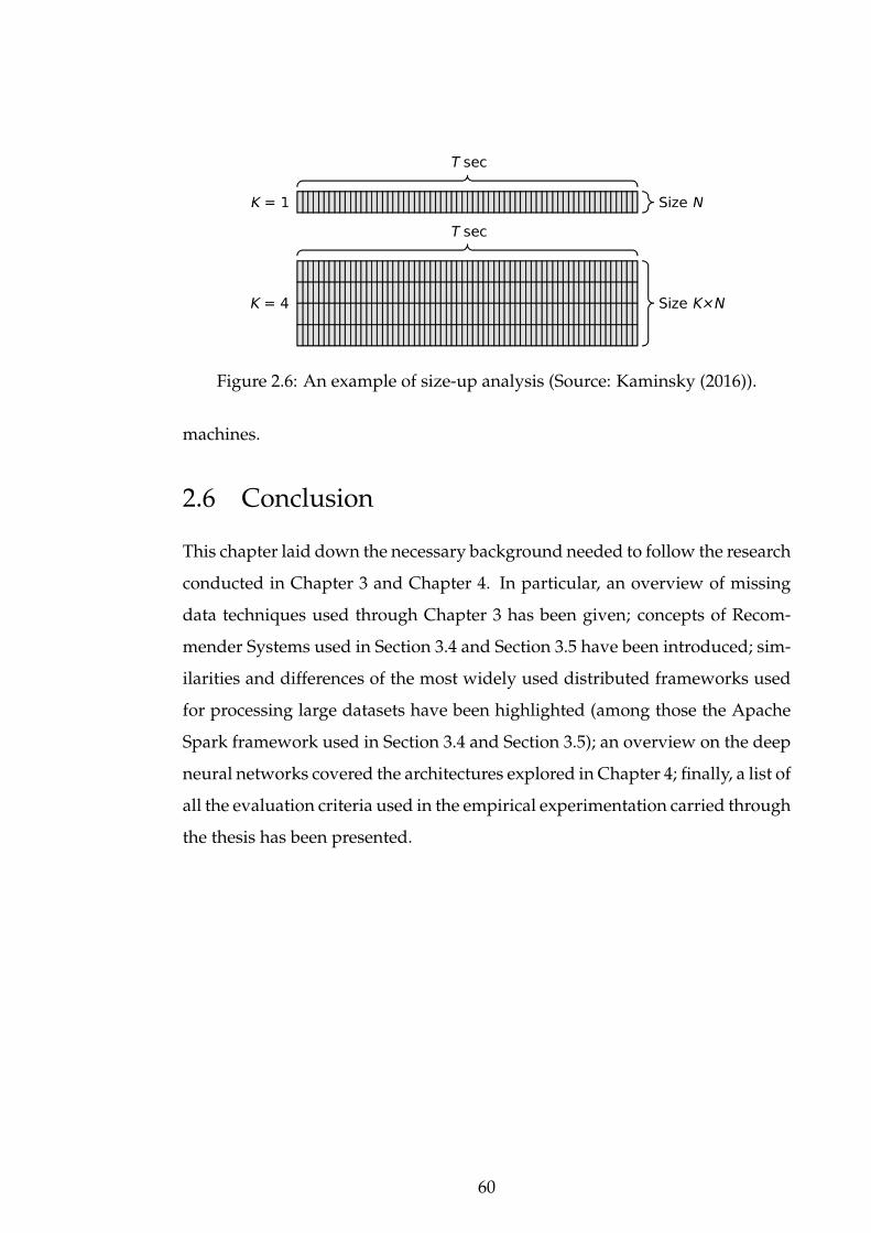
Figure 2.6: An example of size-up analysis (Source: Kaminsky (2016)).

machines.

2.6 Conclusion

This chapter laid down the necessary background needed to follow the research

conducted in Chapter 3 and Chapter 4. In particular, an overview of missing

data techniques used through Chapter 3 has been given; concepts of Recom-

mender Systems used in Section 3.4 and Section 3.5 have been introduced; sim-

ilarities and differences of the most widely used distributed frameworks used

for processing large datasets have been highlighted (among those the Apache

Spark framework used in Section 3.4 and Section 3.5); an overview on the deep

neural networks covered the architectures explored in Chapter 4; finally, a list of

all the evaluation criteria used in the empirical experimentation carried through

the thesis has been presented.

60

3 Missing Data Imputation

In this chapter I tackle the missing data problem and its impact in small and

big data. The literature review (Section 3.1) gives an overview of works inves-

tigating and comparing a variety of techniques, trying to find the best one for a

given task (e.g., regression, classification, etc) and field of application (e.g, ge-

netics, environment, etc). Following the literature review I focus on three gaps

in missing data imputation: the “no free lunch theorem” for missing data impu-

tation (i.e., there is no single method always able to outperform all the others);

the missing data problem in Recommender Systems (also known as cold start

problem); and the missing data problem at scale for big datasets.

After an initial study of missing data techniques in Section 3.2, I propose a fea-

ture based imputation technique which learns, for each in a dataset, the most

suitable imputation technique (Section 3.3). Following, in Section 3.4, I investi-

gate the impact of missing data in a real-world Recommender System ranking

Online Travel Agency properties (i.e., hotels, motels, vacation rentals). Lastly, I

introduce a novel imputation technique scaling to big datasets not fitting in the

memory of one machine (Section 3.5).

3.1 Literature Review

A variety of imputation techniques has been used and implemented in the past

years, e.g. Musil et al. (2002) compared five approaches (i.e., list-wise deletion,

mean imputation, simple regression, regression with an error term, and the EM

algorithm) on a relatively small dataset (450 patterns) with 20% of MAR. The

mean imputation appeared the least accurate method and the EM was the most

accurate, however, the authors addressed some limitations in approximating

the original data for all compared methods. Shrive et al. (2006) used a survey

dataset (1580 participants and 20 ranked questions) with 10% to 30% of artificial

missing data to compare six imputation techniques (i.e., MI, single regression,

individual mean, overall mean, participant’s preceding response and random

selection) under MAR and MNAR assumption. The MI achieved the best ac-

61

curacy for some of the experiments, followed by the individual mean. Again

there was not just one imputation technique that outperforms all the others, and

the authors stated that a good imputation method should balance accuracy and

interpretability of the results. Chang and Ge (2011) compared ten imputation

methods for handling missing value problem of micro-array data with bPCA,

on the imputation of traffic flow data. The authors carried out this comparison

to show that other methods (i.e., LSI gene, LSI array, LSI combined, LSI adap-

tive, EM gene and local least square imputation) can be more accurate than the

bPCA, which is assumed to outperform most of the conventional approaches

(i.e., KNNI and EM methods). The RMSE was used to compare the methods

performance over datasets with 2% to 50% missingness rates. Liu and Brown

(2013) used a dataset of 100 artificial patterns (50 elements with mean vector

[1,0] and 50 with [-1,0]), and two small real-world datasets (i.e., Iris and Wine)

to compare five iterative imputation methods (i.e., general iterative principal

component imputation, singular value decomposition imputation, regularized

EM with multiple ridge regression (r-EM), regularized EM with truncated to-

tal least squares, and MICE) on a multivariate analysis and classification prob-

lem. Instead of using the canonical imputation metric (e.g., MAE or RMSE) and

classification accuracy, the authors introduced two new metrics, namely covari-

ance criterion and classification criterion, which assess the change in the covari-

ance matrix and the change in the classification error caused by the imputation.

However, it is important to bear in mind that the population covariance and

class assignments are usually unknown for practical, incomplete data. The au-

thors concluded that no single imputation method emerged as the overall best

in all examined cases. Judging from the obtained results from both real-world

datasets, the r-EM imputation method was considered the best when the miss-

ingness rate is under 20%. For the cases with above 20%, the authors suggested

careful consideration whether an imputation should be applied at all. Gomez-

Carracedo et al. (2014) compared five imputation methods (i.e., list-wise dele-

tion, unconditional mean, modified mean, principal component based imputa-

tion, EM and MI) on three air quality datasets with missingness rate between

4% and 24%. All the considered techniques performed similarly in this investi-

62

gation, although MI substituted values with larger variance, mostly attributed

to the high rate of missingness, while the rest of the techniques estimated values

with smaller variance. Schmitt et al. (2015) compared six imputation methods

(i.e., mean imputation, KNNI, FKM, SVDI, bPCA and MICE) over four datasets

and four performance measures (i.e., RMSE, unsupervised classification error,

supervised classification error and execution time). Accordingly with Oba et al.

(2003), bPCA outperformed mean imputation, KNNI, SVDI and MICE; while

FKM was better than bPCA in all the metrics but the execution time, which can

be considered a possible drawback in case of large datasets. All these reviewed

works compared the algorithms trying to identify the one achieving the best

overall accuracy for each dataset. The ensemble method (Dietterich, 2000) al-

ready showed good results when applied to other fields of machine learning,

as in classification tasks (Breiman (2001)’s random forests) and in optimization

problems (e.g., genetic algorithms (Wang et al., 2014; Petrozziello et al., 2017)).

Similar results have been achieved when different imputation methods were

ensembled to improve the estimation accuracy (Twala et al., 2006; Sorjamaa and

Lendasse, 2010; Pan et al., 2011). Twala et al. (2006) used an ensemble of seven

imputation algorithms (LD, EMSI, kNNSI, MMSI, EMMI, FC, and SVS) on eight

small software effort estimation datasets (18 to 166 instances) with artificial

MCAR and MAR. The experiment was done under a 5-fold cross validation;

the ensemble was created through randomized decision trees and a training

set was used to select the combination of two algorithms with the smallest er-

ror. Sorjamaa and Lendasse (2010) applied an ensemble of Self-Organized Map

(SOM) weighted with nonnegative least squares algorithm to impute data on

two real-world datasets, namely Corporate Finance and Climatology. The al-

gorithm was compared with four imputation methods (Empirical Orthogonal

Functions (EOF), EOF Pruning, Probabilistic PCA and single SOM). The assess-

ment of the results was carried out comparing the MSE on the test set and the

execution time. In both cases the ensemble of SOM achieved the lowest error

and smaller computational time since calibration of the model through the vali-

dation phase was skipped. Pan et al. (2011) used an ensemble of six imputation

methods (bPCA, Matrix CompletionMC, LLS, uKNN, wKNN, and LSimpute)

63

over six epistatic mini-array profiling datasets. Despite the good results, the

ensemble was done via a weighted linear combination of the five methods, pre-

determining one of the algorithms as a reference and calculating the individual

diversities of the other five algorithms.

As can be observed by the literature review, the proposed methodologies are

often only tested on small datasets comprising up to a few thousands records.

Furthermore, the majority of imputation techniques described in Section 2.1

only work as long as the full dataset can be stored in memory, which would con-

stitute a problem for datasets containing hundreds of thousands of records (i.e.,

tall datasets), hundreds of features (i.e., wide datasets), or both. Little research

has been done in the field of missing data imputation for big data. In the case

where the missing rate is negligible compared to the size of the dataset, a dele-

tion method is applicable without losing statistical strength. However, if the

rate of missingness grows with the size of the dataset the imputation is neces-

sary to preserve, or even increase, the statistical power of the data. The few ad-

vances in the field happened during the last couple of years have been possible

due to the rising interest in distributed processing frameworks. Anagnostopou-

los and Triantafillou (2014) use a Map-Reduce-like approach to scale the miss-

ing values imputation problem adopting the concept of signature (the record is

assigned to a cluster based on its features value) and data locality (the record

is allocated to the machine handling that specific cluster). Once the record has

been allocated to the machine, a missing data technique can be locally used to

impute its missing values. The proposed framework has been tested on two real

datasets (namely D1 and D2) and one synthetic. The D1 dataset is composed

of 500K samples and 90 features, while D2 has 50K records and 384 variables.

The synthetic dataset has 20 features, five of which with missing values. The

records for this dataset are generated on the fly and assigned to each machine

to perform the imputation step. The authors show that it is possible to reduce

the imputation time, and make the imputation feasible even for large datasets,

distributing the computation on a cluster of machines. However, the impact on

the imputation accuracy would depend on the chosen granularity (i.e., number

64

of machines) and the signature function (i.e., clustering technique). Singh and

Toshniwal (2019) propose a data decomposition approach for RBF functions on

Spark. The authors use a divide and conquer approach which split the data in

small overlapping windows. Firstly the data are sorted applying an Euclidean

distance on the features; secondly, for each window, an imputation model is

trained; and lastly, all models are aggregated to get a global one. Although the

model has been tested on eight datasets coming from the UCI repository, the

biggest one utilized has less than fifty thousands records. As in the previous

study, results showed that the the trade-off between accuracy, speed and fea-

sibility is driven by the number of windows - with bigger windows yielding

better generalization, while being constrained by the memory size.

3.2 Radar Signal Recognition with Missing Data

This section addresses a classification task for recognition of intercepted radar

signals with high percentage of records containing missing values (Jordanov

et al., 2016, 2018). The problem is to classify the signals into several functional

groups by finding patterns in their pulse features (i.e., frequencies, modulation

types, pulse repetition, scanning period, etc). To recover the missing data, three

main approaches namely Multiple Imputation (MI), K-Nearest Neighbours Im-

putation (KNNI) and Bagged Tree Imputation (BTI) are investigated, tested and

validated on two case studies: binary classification and multi-class classifica-

tion. Three different classifiers (i.e., Random Forests (RF), Neural Networks

(NN) and Support Vector Machines (SVM)) are then trained to solve the sig-

nal classification problem. Each of the approaches is tested and validated on a

number of case studies and the results are evaluated and critically compared.

3.2.1 Background

Radar activity is generally grouped in two areas of application: military and

civil. In the military sector, radar activity has found application in surveillance,

navigation, and weapon guidance, while in the civil are, radars are widely used

for traffic control, navigation, weather forecast, pollution control, space obser-

65

vation, and others (Richards, 2005; Jordanov and Petrov, 2016). The radar char-

acteristics (i.e., range, resolution and sensitivity) are determined by its transmit-

ter and waveform generator: most of the radars operate within the microwave

region of the electromagnetic spectrum (with frequency ranging 200 MHz to

95 GHz), and are used for short range application with high resolution; other

radars operate at a very low frequency bands and are usually preferred to cover

longer distances (Richards, 2005). Radar classification and tracking of targets

against a background of clutter are considered as a “general radar problem”.

For military purposes it includes interception, localisation, analysis and iden-

tification of radiated electromagnetic energy, also known as radar Electronic

Support Measures (ESM). A real-time identification of the radar emitter associ-

ated with each intercepted pulse train is a very important function of the radar

ESM. Typical approaches include sorting incoming radar pulses into individ-

ual pulse trains and comparing their characteristics with a library of paramet-

ric descriptions in order to get a list of likely radar types. This task is very

difficult as there may be radar types with no records in the ESM library; over-

laps of different radar parameters for the same type; increases in environment

density; noise and propagation distortion that lead to incomplete or erroneous

signals (Granger et al., 2001). Intercepted and collected pulse train character-

istics typically include signal frequencies, type of modulation, pulse repetition

intervals, etc. The collected information usually consists of a mixture of con-

tinuous, discrete and categorical data with frequent missing values (Table 3.1).

Handling such high rate of missing data is a very important part of the data pre-

processing before applying classification models (Saar-Tsechansky and Provost,

2007).

Table 3.1: Sample radar data. Missing values (i.e., values that could not havebeen intercepted or recognized) are denoted with “-”. The rest of the acronymsare defined in Table 3.3.

ID FN RFC RFmi RFma PRC PRImi PRIma PDC PDmi PDma ST SPmi SPma84 SS B 5300 5800 K - - S - - A 5.9 6.1

4354 AT F 2700 2900 F 1351.3 1428.6 S - - A 9.5 10.5 -7488 3D B 8800 9300 K 100 125 S 13 21 B 1.4 1.69632 WT F 137 139 T - - V - - D - -9839 3D S 2900 3100 J - - V 99 101 A 9.5 10.5

66

Table 3.2: Sample radar subset with imputed continuous values.

ID FN RFC RFmi RFma PRC PRImi PRIma PDC PDmi PDma ST SPmi SPma84 SS B 5300 5800 K 963.2 5625 S 5.8 17 A 5.9 6.1

4354 AT F 2700 2900 F 1351 1428 S 4 6.3 A 9.5 10.57488 3D B 8800 9300 K 100 125 S 13 21 B 1.4 1.69632 WT F 137 139 T 622.6 31312 V 61.1 93.1 D 12 47.89839 3D S 2900 3100 J 2058 48128 V 99 101 A 9.5 10.5

3.2.2 Data pre-processing

The original dataset includes about 30000 sample of which 7693 fully inter-

cepted and recognised radar signals that constitutes the complete subset (after

applying list-wise deletion of the original dataset) (Jordanov and Petrov, 2014).

As suggested in the literature, it is recommended to exclude samples containing

more than 50% of missing values, for this reason, from the samples with missing

data (example given in Table 3.1) I excluded those with above 60% missingness

(as previously done in Jordanov and Petrov (2014)), which brought the dataset

to 22000 samples and used MI, KNNI, and BTI for substituting the rest.

The data imputation with MI led to a dataset of 15656 samples - hence doubling

the number of the available data (Table 3.2 shows the samples from Table 3.1

with the imputed values produced by the MI).

On the other hand, when using KNNI and BTI, all missing data were recov-

ered, enabling us to utilise valuable information and use the statistical power

of the data contained in the samples with missing values. As can be seen from

Table 3.1, the first column includes the data sample identifier, the second shows

the category label (the output of the classifier) and the rest of the table contains

radar signal pulse train characteristics (the classifier’s inputs). A more com-

prehensive summary of the data distribution is presented in Table 3.3, where

an overview of the type, range and percentage of missing values for each pa-

rameter is given. The analysed data consists of both numerical (discrete and

continuous) and categorical values, the latter of which are coded during the

data pre-processing stage, converting them into numerical features. As can be

seen from the table, the percentage of missingness varies from 11.2% for the

radar frequency feature (RFmi) to 59.4% for the scan period characteristic (SP).

67

Table 3.3: Data description and percentage of missing values.Type: I - integer; C - categorical; R - real values.

Field Field Description Type Levels % MissingID Reference for the line of data I - -FN Function performed by the radar (3D - 3D surveillance,

AT - air traffic control, SS - surface search, WT - weather tracker, etc.)C 142 1.4

RFC Type of modulation used by the radar to change the frequencyfrom pulse to pulse (A - agile, F - fixed, etc.)

C 12 20.7

RFmi Min frequency used by the radar R - 11.2RFma Max frequency used by the radar R - 11.2PRC Type of modulation used by the radar to change

the Pulse Repetition Interval (PRI), (F - fixed, etc.)C 15 15

PRImi Min PRI used by the radar R - 46.7PRIma Max PRI used by the radar R - 46.7PDC Type of modulation used by the radar to change

the pulse duration (S - stable)C 5 12.9

PDmi Min pulse duration used by the radar R - 46.1PDma Max pulse duration used by the radar R - 46.1ST Scanning type - used method by the radar to move the antenna beam

(A - circular, B - bidirectional, W - electronically scanned, etc.)C 28 11.3

SPmi Min scan period used by the radar R - 59.4SPma Max scan period used by the radar R - 59.4

Verboven et al. (2007) sequential imputation algorithm is used for MI, imple-

mented in the impSeq function from the rrcovNA R package (its robust version

impSeqRob was also tested; but it didn’t produce better results probably due to

the lack of outliers). For the KNNI, a K = 10 is used as advised by Batista and

Monard (2002), while for BTI Ridgeway (2007) R gbm package is leveraged to

implement the imputation function.

The pre-processing of the available data is of a great importance for the sub-

sequent machine learning stage as it can affect significantly the overall success

or failure of the used classification algorithm. This stage of the pre-processing

aims to transform the data into a form suitable for feeding to the selected clas-

sifier, expecting to facilitate faster and more accurate machine learning train-

ing. The categorical features in the dataset are transformed into numerical ones.

Three of the most broadly applied coding techniques are investigated and eval-

uated here: continuous; binary; and dummy variables. For the first type of cod-

ing, each category is substituted with a natural number, e.g., the 12 categories

for the RFC input are encoded with 12 ordinal numbers, the 15 PRC categories -

with 15 ordinal numbers, etc. A sample of a data subset coded with continuous

values is given in Table 3.4. Binary coding, wherein each non-numerical value

is substituted by log2N new binary variables (where N is the number of cate-

68

gories), is illustrated with 32 categories in Table 3.5. Finally, the non-numerical

attributes are also coded using dummy variables (also known as one-hot encod-

ing), where every level of a categorical variable is represented by a new unique

variable. An example of one-hot encoding coding for 32 levels is shown in Ta-

ble 3.6. In order to mitigate the impact of difference in magnitude of the inputs

on the training algorithm, the data is scaled during the pre-processing phase.

Correspondingly, each of the conducted experiments is evaluated using three

forms of the input dataset: the original data (i.e., no scaling); normalized data

(i.e., normalizing each feature within (0, 1) interval); and standardized data (i.e.,

standardizing the feature space with 0-mean and a unit variance).

For the identification and classification of the radar signals, the applied super-

vised learning uses from two to eleven output classes: in the first set of simu-

lations I use 2 classes - civil and military (defined by experts in the field from

a total of 125 functional categories); and in the second set of simulations, four

civil and seven military classes, which gives eleven output labels to classify.

Table 3.4: Sample subset with imputed radar data and natural number codingof RFC, PRC, PDC, and ST.

ID RFC RFmi RFma PRC PRImi PRIma PDC PDmi PDma ST SPmi SPma84 2 5300 5800 7 963.2 5625 1 5.8 17 1 5.9 6.1

4354 4 2700 2900 4 1351 1428 1 4 6.3 1 9.5 10.57488 2 8800 9300 7 100 125 1 13 21 2 1.4 1.69632 4 137 139 11 622.6 31312 2 61.1 93.1 4 12 47.89839 9 2900 3100 6 2058 48128 2 99 101 1 9.5 10.5

Table 3.5: Example of binary coding for 32-level categorical variable.

Label Encoded VariablesIndex Label B1 B2 B3 B4 B5

1 2D 0 0 0 0 02 3D 0 0 0 0 13 AA 0 0 0 1 0... ... ... ... ... ... ...16 CS 0 1 1 1 1... ... ... ... ... ... ...32 ME 1 1 1 1 1

69

Table 3.6: Example of dummy coding for 32-level categorical variable.

Label Encoded VariablesIndex Label D1 D2 D3 D4 D5 ... D16 ... D32

1 2D 1 0 0 0 0 ... 0 ... 02 3D 0 1 0 0 0 ... 0 ... 03 AA 0 0 1 0 0 ... 0 ... 0... ... ... ... ... ... ... ... ... ... ...16 CS 0 0 0 0 0 ... 1 ... 0... ... ... ... ... ... ... ... ... ... ...32 ME 0 0 0 0 0 ... 0 ... 1

3.2.3 Supervised radar classification techniques

There is a wide variety of approaches and methods used for radar emitter recog-

nition and identification. Among those, Neural Networks, Support Vector Ma-

chine and Random Forest have been independently investigated in previous

study and for this reason are here compared.

a) Neural Networks

Various approaches and methods have been investigated and used for radar

emitter recognition and identification, and considerable part of this research

incorporates Neural Networks (NN).

NN techniques have previously been applied to several aspects of radar ESM

processing and more recently, many new radar and target recognition systems

include neural networks as a key classifier (Gong et al., 2016). Examples of a

variety of NN architectures and topologies used for radar identification, recog-

nition and classification based on ESM data include popular multilayer per-

ceptron, radial basis function (RBF) based NN, vector NN, single parameter

dynamic search NN (Ibrahim et al., 2009; Ahmadlou and Adeli, 2010; Yin et al.,

2011) and deep NN (Gong et al., 2016). For example, Granger et al. (2001) use

initial clustering algorithm to separate pulses from different emitters according

to position-specific parameters of the input pulse stream when implementing

their “What-and-Where fusion strategy” and then apply fuzzy ARTMAP-NN

to classify streams of pulses according to radar type, using their input parame-

ters. They also do simulations with dataset that has missing input pattern com-

ponents and missing training classes and incorporate a bank of Kalman filters

70

to demonstrate high level performance of their system on incomplete, overlap-

ping and complex radar data. Ibrahim et al. (2009) investigate the potential of

multilayer perceptron when used in “forward scattering radar applications” for

target classification. The authors analyse collected radar signal data and extract

features, which are then used to train NN for target classification. They also

apply the KNN classifier to compare the results from the two approaches, con-

cluding that the NN solution is superior. Shieh and Lin (2002) use a vector NN

for emitter identification while Gong et al. (2016) used deep NN architectures

for synthetic-aperture radar images recognition. In many cases the NN are hy-

bridized with fuzzy systems, clustering algorithms, wavelet packets, Kalman

filters, particle swarm optimization-based SVM, etc., which in turn leads to sys-

tems with increased accuracy (Granger et al., 2001; Shieh and Lin, 2002).

b) Support Vector Machines

Support Vector Machines (SVM) are a type of learning machines based on the

statistical learning theory, that can use linear, polynomial, Gaussian, exponen-

tial and hybrid kernels for the classification. RBF networks, and even particle

swarm optimisation has been used in some cases (Zhai and Jiang, 2015). SVM

maximize the error margin between the classes searching for an optimal clas-

sification hyperplane in a higher dimensional space of the features. In other

words if the feature space is linearly non-separable, the SVM use non-linear

mapping to find a better discriminant hyperplane. The choice of a map func-

tion (kernel) is of critical importance and can substantially determine the clas-

sification results (Xin et al., 2010). One advantage of this approach is that it

is possible to design and use a kernel for a specific problem that could be ap-

plied to the data without the need of a feature extraction process. The SVM

have been used recently to classify radar pulse signals. For example, Eryildirim

and Onaran (2011) use SVM to classify targets by using micro-Doppler features

when analysing micro-motions of an object having single signature. Target

recognition method based on SVM with hybrid differential evolution and self-

adaptive particle swarm optimization is investigated by Zhai and Jiang (2015),

reporting low error rate on the given task. Implementations of SVM exist in

71

almost every programming language and at least four R packages contain SVM

related software (I used the R package E1071 which I found to work faster on

multi-class problems (Karatzoglou et al., 2005)).

c) Random Forests

Random Forests (RF) is a powerful machine learning technique that operates by

constructing a multitude of decision trees at training time and outputs the class

that is the mode of the classes (classification) or mean prediction (regression)

of the individual trees. Each tree is trained on a bootstrapped sample of the

training data, and at each node, the algorithm only searches across a random

subset of the variables to determine a split. For an input vector to be classified,

it is submitted to each of the decision trees in the forest and the prediction is

then formed using a majority vote. Key advantages of the RF include: their

non-parametric nature; avoiding decision trees’ habit of overfitting; high clas-

sification accuracy; and capability to determine variable importance (Breiman,

2001). However, as the split rules for classification are unknown, the RF can be

considered to be a black box type classifier. In this implementation, I used the

randomForest function (from the R randomForest package), which implements

the Breiman’s random forests algorithm.

3.2.4 Assessment baseline

To begin with, it is essential to determine which imputation method leads to

the best substitution of the missing values. For this purpose, I designed two

experiments, as described below.

a) Labels Imputation

In order to test the reliability of the investigated imputation models, 25% of

the labels in the complete data subset (around 4000 samples), are randomly

removed. The labels are subsequently imputed, using the three methods: MI,

BTI and KNNI. Considering the random nature of the algorithms, I run the

imputation 30 times for each of them. This is done for the two simulations:

with 2 classes and with 11 classes. In the 2-class imputation case, the KNNI

72

method achieved the best performance with a 90% accuracy, followed by BTI

with 84% and MI with 65% (Figure 3.1).

MI BTI KNNI

0.65

0.75

0.85

Imputation Method

Accu

racy

(%)

Figure 3.1: Label imputation for MI, BTI and KNNI over 30 runs for 2 classes.Each boxplot displays the minimum and maximum values (whiskers), the firstand the third quartile (boundaries of the box represent 50% of the data), andthe median (the thick line).

The KNNI achieved the best accuracy most likely due to the skewed nature

of the data: in fact, 75% of the data belongs to the second class, this way, the

unbalanced dataset helps the search of nearest neighbours to go towards the

class with more samples. On the contrary, the MI and BTI methods assume

balanced label distribution, which leads to limited accuracy of their imputation.

In the 11-class case (Figure 3.2), the effect is even more evident, as the samples

are not equally distributed among the classes, leading to a low accuracy for

MI and BTI and a high variance for KNNI due to the randomness of the labels

removed in each of the 30 runs.

b) Continuous features imputation

The second experiment aims to validate the algorithms’ accuracy in presence

of continuous features. Eight features from the complete subset (RFmi, RFma,

PRImi, PRIma, PDmi, PDma, SPmi, SPma) are considered in this setup. As in

the previous experiment, 25% of the data is removed for each feature and sub-

sequently imputed. The RMSE between the imputed values and the real ones

is selected to measure the methods’ performance. The experiment is iterated

73

MI BTI KNNI

0.1

0.3

0.5

0.7

Imputation Method

Accu

racy

(%)

Figure 3.2: Label imputation for MI, BTI and KNNI over 30 runs for 11 classes.Each boxplot displays the minimum and maximum values (whiskers), the firstand the third quartile (boundaries of the box represent 50% of the data), andthe median (the thick line).

30 times and the Wilcoxon test for statistical significance (with ↵ < 0.05) along

with the relative Cohen’s d effect size, are calculated.

The considered imputation algorithms are also tested against the median im-

putation as a comparison baseline. As expected (Figure 3.3), all other algo-

rithms outperformed the median imputation, producing smaller errors. In 23

out of 25 cases BTI is significantly better than MI and KNNI and with effect size

d=1. The comparison between BTI and KNNI on PRImi and PRIma, despite a

p-value < 0.025, showed slightly lower effect size, d=0.83 and d=0.78 respec-

tively. Analysing the results for the two features led to the conclusion that

the KNNI is again strongly affected by the data distribution, which is highly

positively skewed for PRImi and PRIma (Figure 3.4). Figure 3.4 shows the nor-

malized density function for four features, from which PRImi and PDmi have

high positive skewness, concentrated in the first quartile. It seems, as for the la-

bel imputation, that a highly imbalanced distribution can affect the imputation

process, explaining why each imputation method produces different accuracy

for the features given in Figure 3.3 (although, BTI is the overall winner). The

results for the Wilcoxon test subjected to the Benjamini-Hochberg and Bonfer-

roni corrections (Dalgaard, 2008) for multiple statistical test are still significant

74

(↵ = 0.05).

MI BTI KNNI Median

1000

1500

2000

RFmiRMSE

MI BTI KNNI Median

400

500

600

700

800

PRImi

RMSE

MI BTI KNNI Median

1.0

1.5

2.0

2.5

PDmi

RMSE

MI BTI KNNI Median

0.8

1.0

1.2

1.4

1.6

1.8

SPmiRMSE

Figure 3.3: Root mean square error (RMSE) for the imputation of the contin-uous values (30 runs). Low median values represent preferable imputationmethods. Non-overlapped boxplots indicate statistical difference between thealgorithms. For a better visualisation, the features RFma, PRIma, PDma andSPma have been omitted due to the similar distribution and high correlationwith the respective minimum.

3.2.5 Classification results

Two main experiments are conducted for investigating the efficiency of each

classifier when solving the radar emitter recognition problem. The dataset is

split into two subsets before the imputation: one for training (75% of the whole

data) and second one for testing (25% of the whole data). The investigated neu-

ral network topologies include one hidden layer with fully connected neurons

in the adjacent layers and batch-mode training is performed. For a given exper-

75

Figure 3.4: Density function for the features: RFmi, PRImi, PDmi, SPmi on thedataset without missing value. Each feature is normalized within (0, 1) interval.The distribution of PRImi and PDmi shows highly positive skewness. For abetter visualisation, the features RFma, PRIma, PDma and SPma are omitteddue to the similar distribution and high correlation with the respective minima.

iment with P learning samples, the error function is given by:

Ep =12

PX

p=1

LX

i=i

(xpi - tpi )2 , (29)

where for each sample p = 1, ...,P and each neuron of the output layer i =

1, ...,L; a pair (xi, ti) of NN output and the target values is defined respectively.

NN learning with Levenberg-Marquardt algorithm is then used and the train-

ing set is further divided into 80% for the training and 20% for the validation.

The MSE is used for evaluating the NN learning performance. The stopping

criterion is set to 500 training epochs, or gradient reaching value less than 1.0e-

06, or 6 consequent failed validation checks, whichever occurs first. For the

RF, the limit for the number of trees is set to 500 and the output class is de-

cided by a vote among them. The SVM are provided with a radial basis kernel

(other kernels were tried as well but led to worse results) and the algorithm

hyper-parameters are optimised through the tune.svm function included in the

76

(a) (b)

Figure 3.5: Figure 3.5a Confusion matrix illustrating the RF classification resultsfor the two classes, after using BTI with continuous value coding (Military andCivil). Figure 3.5b ROC Curve for the same simulation.

package, which increased the classifier accuracy with up to 4%.

For the first experiment, the NN topology is N-N-2, where N is the number of

inputs and the output contains 2 binary neurons coded as: 10 for class Civil; and

01 for class Military. For the second experiment, the same topology is used with

11 output neurons (representing 4 civil and 7 military classes). After coding the

categorical variables with the three methods described above, the accuracy of

each classifier is investigated, evaluated and compared before and after the data

normalisation and standardisation.

Sample confusion matrices are shown for the best accuracy achieved in the ex-

periments for the 2 and 11 classes, after training with continuous input data.

The RF demonstrates high accuracy, as can be seen from Figure 3.5a and Fig-

ure 3.6, showing the number of correct responses in the green squares and the

number of incorrect responses in the red squares. The bottom right percentage

illustrates the overall classifier accuracy (OCA) described in Eq. 11. Further-

more, it can be observed from Figure 3.6 that the number of hits, as well as

the accuracy of the RF classifier, compared to the previous work (Jordanov and

Petrov, 2014), has increased. Another important achievement is also illustrated

in these figures: the class accuracy variance of the classification is now within

the 34.8% to 90.8% interval; while in (Jordanov and Petrov, 2014) it was between

22.6% and 87.4%. This may be attributed to the higher number of available

77

Figure 3.6: Confusion matrix illustrating the RF classification results for the 11classes, after using BTI with continuous value coding. The batch includes 7military (M1 - Multi-function, M2 - Battlefield, M3 - Aircraft, M4 - Search, M5 -Air Defence, M6 - Weapon and M7 - Info) and 4 civil classes (C1 - Maritime, C2- Airborne Navigation, C3 - Meteorological, C4 - Air Traffic Control).

training and testing samples as a result of the BTI imputation, which increased

the used dataset statistical power and improved the classification performance

of the RF. The results shown in Figure 3.7 and Figure 3.8, illustrate moderate

impact of the categorical coding on the classification. The continuous coding

appears to be more efficient (1% better for the 2-class case, and 5% for the 11-

class one). For the 2 classes, the best result (90.80%) is obtained when combining

the RF classifier with the BTI and continuous values, and for the 11 classes, the

same combination achieved again the best accuracy of 71.0% (Figure 3.6).

In Figure 3.7 and Figure 3.8, the SVM columns (the last three columns) have the

same results for the scaled and standardized data, since the algorithm performs

internally the two operations before the classification. In 98 out of 108 compar-

isons, BTI has demonstrated the best accuracy for all classifiers, while the KNNI

achieved best results in 8 cases and MI in 2 comparisons only. Taking a closer

look at the confusion matrix given in Figure 3.6, it can be seen that the num-

78

Figure 3.7: Classification performance results of the classifiers (RF, NN andSVM) in the case of 2 classes after using three different imputation techniques(BTI, KNNI and MI), for the three different groups of coding (binary, contin-uous and dummy). The colour scale to the left shows the achieved accuracypercentile.

ber of misclassified samples within the classes of the same family (e.g., civil)

is higher than the number of misclassified samples as belonging to the other

family classes (e.g., military). For example, if we take a look at M1 class (5th

row in Figure 3.8), 24 samples of M1 class are wrongly classified as belonging

to civil classes (C1 to C4), while 63 samples are mislabelled as of the other mili-

tary classes (M2 to M7). It is even more evident from the last row (M7 class), for

which all misclassified samples (seven) belong to the military family. Since it is

not possible to give a cost for the misclassification of each class, a ROC curve

analysis for multiclass problems is used to assess the classifiers accuracy under

different conditions. Let’s call a superclass the union of all classes belonging to

the same general type or family (civil or military) for the 11-class problem: C =

[(C1,..., C4); and M = [(M1,..., M7). I also define two types of misclassification

errors: outer error (OE) and inner error (IE).

In the 11-class case, the OE occurs when: one of the civil samples belonging

79

Figure 3.8: Classification performance results of the classifiers (RF, NN andSVM) in the case of 11 classes after using three different imputation techniques(BTI, KNNI and MI), for the three different groups of coding (binary, contin-uous and dummy). The colour scale to the left shows the achieved accuracypercentile.

to a Ci, i = 1,..., 4, class is misclassified as belonging to a military one Mj, j

= 1,...,7; or when a military sample is mislabelled as a civil one. An IE occurs

when a civil sample is misclassified as belonging to another civil class or when a

military pattern is mislabelled with a different military label. Let’s now denote

the inner accuracy (IA) as the accuracy obtained calculating the ROC curve for

a multi-class problem, as proposed by Hand and Till (2001), when applied only

on classes belonging to the same superclass. In (Hand and Till, 2001), the area

under the curve (AUC) is obtained by averaging the AUC of all considered

pairwise classes. This approach measures how well each class is separated from

the others, emphasising that certain pairs of classes can be well separated, even

when the superclasses cannot be well separated.

Labelling the civil classes C1, ..., Ck, (k = 4), I estimate the probability of each

test sample x belonging to any class Ci as: p(Ci|x), for i = 1, ..., k. For any pair

of classes (Ci, Cj), it is possible to compute measure A using p(Ci|x) or p(Cj|x),

80

hence, A(Ci|Cj) is the probability of a randomly selected member of class Ci

to have lower estimated probability of belonging to class Cj, than a randomly

selected member of class Cj. Because for a 2-class problem (class 0 and class

1): A(0|1) = A(1|0); and for a multi-class problem A(Ci|Cj) 6= A(Cj|Ci), I use the

average A(Ci, Cj) = (A(Ci|Cj) + A(Cj|Ci) )/2, adopted as measure of separability

between Ci and Cj. The overall performance of the classification in separating

k classes is then the average of this measure over all class pairs:

IA =2

k(k- 1)(X

i<j

A(Ci,Cj) +X

i<j

A(Mi,Mj) . (30)

The difference 1 - IA represents on average, the percentage of wrongly labelled

patterns in the same superclass. On the other hand, the outer accuracy (OA) is

calculated applying the average AUC to all the pairs (Ci, Mj)

OA =

PA(Ci,Mj)

kn, (31)

where i = 1, ...,k, j = 1, ...,n, and k and n are the number of civil and military

classes respectively. Again, the difference 1 - OA represents the percentage of

patterns, misclassified as belonging to the other superclass.

Results for IA, OA and OCA are given in Table 3.7, where in the first six rows

the best OA and OCA accuracies for the RF, NN and SVM classifiers are shown

(which performance is illustrated with Figure 3.8). The last two rows display

the results for NN (with MI and continuous coding) and SVM (with BTI, binary

coding and standardisation). The IA and OA can help to better understand the

underlying distribution of the misclassified samples among the classes. Look-

ing at the results in Figure 3.8, it is evident that for some of them, it is difficult

to choose the best classifier due to the similar OCA values. In such cases the

OA can provide insightful information and help identify the best one. For ex-

ample, the OCA is identical (46%) for the NN (with MI and continuous coding)

and SVM (with BTI, binary coding and standardization) classifiers. Neverthe-

less, looking at the OA column in Table 3.7 (last 2 cells), one can see that the

81

NN classifier has 11.1% better accuracy than the SVM one. In theory, it may

be speculated that the probability of having a misclassified sample within the

same superclass is higher (since they are coming from the same family of radar

signals), than the probability of class being misclassified as belonging to the

other superclass. Considering the values given in Table 3.7, it can be seen that

the IA is generally lower than the OA, which is in agreement with the above

presumption. Moreover, the RF, NN and SVM classifiers producing the best

OCA (71%, 54.9%, and 47.6%: rows 2, 4, and 6, respectively) are not the best

ones when OA is used as a metric (then their OCA are 68.3%, 52.7%, and 46.2%:

rows 3, 5, and 7, respectively). This enforces the point that a second metric

should be used when assessing classifiers performance.

Table 3.7: Classifiers Inner Accuracy (IA) and Outer Accuracy (OA) comparedto the best Overall Classifier Accuracy (OCA) in the 11 class classification forRF, NN and SVM; best OA for RF, NN, SVM; and results for two classifiers withsame OCA but different OA.

Classifier IA OA OCARF BTI continuous (RFbest OCA) 87.1 88.7 71.0RF KNNI continuous standardised (RFbest OA) 89.1 90.6 68.3NN BTI dummy scaled (NNbest OCA) 74.1 74.2 54.9NN BTI continuous scaled (NNbest OA) 81.0 84.3 52.7SVM BTI continuous (SVMbest OCA) 64.8 67.7 47.6SVM KNNI continuous scaled (SVMbest OA) 62.9 69.0 46.2NN MI continuous 75.6 78.8 46.0SVM BTI binary standardised 64.9 67.7 46.0

For example, the RF classifiers with highest OCA and OA are shown in the first

2 rows of Table 3.7. In the first (RFbest OCA) case (1st row), 29% of the patterns

are misclassified (1450 of 5000) and 11.3% of them are assigned to the wrong su-

perclass (164 patterns). In the second (RFbest OA) case (2nd row), 31.7% of the

samples (1680 of 5000) are wrongly labelled and 9.4% of them (158) are assigned

to the wrong superclass. As for the NN classifiers (3rd an 4th rows), the differ-

ence in the OCA is very small (2.2%), with 2255 and 2365 misclassified samples

respectively, while the relative OA difference is substantial - 10.1%, with 582

and 371 misclassified patterns respectively. Similar results can be observed for

the SVM classifier as well (6th and 7th rows). As discussed, the use of OA pro-

vides extra insight of the classifiers’ performance, giving additional metric for

82

choosing the best classification model (considering the trade-off between OCA

and OA).

3.2.6 Discussion

The above results showed that the performance of the used classifiers for recog-

nition and identification of radar sources, based on datasets of radar signal

characteristics depends a lot on the quality of the available data and dealing

with the missingness in the datasets can improve the classifier overall accu-

racy. The implementation of imputation models tripled the number of complete

records, which in turn led to improved performance of the classifiers. The BTI

had best accuracy for all supervised classifiers (especially in the 11-class case).

In the 2-class case, the best performance was achieved by the RF after BTI im-

putation and continuous coding (90.8%), followed by the NN (83.3%) and SVM

(81.3%). In the 11-class, I use the ROC curve analysis for a multi-class prob-

lem, and obtain the area under the curve (AUC) by averaging the AUC of all

considered pairwise classes. This approach showed that some pairs of classes

can be well separated, even when the superclasses are not well separated. I

also showed how the two new introduced metrics: inner (super) class error IE

(Eq. 30); and the outer class error OE (Eq. 31), can be used to complement the

OCA metric when choosing the best classifier. Especially in cases when the

OCA has similar values for the classifiers, the OA should be used as an addi-

tional criterion for the choice of the most efficient and accurate method for the

classification. This investigation found that the IE is usually smaller than the

OE, which is in agreement with the presumption that it is more likely a class

to be misclassified for another one from the same superclass (as being from

the same family), than to be misclassified as belonging to the other superclass.

Future work may include identification of more than two superclasses by im-

plementing unsupervised learning and then using supervised one for assessing

IE and OE metrics.

83

3.3 Scattered Feature Guided Data Imputation

All the imputation techniques described in the background section (Section 2.1)

would select a single method that outperforms the others, based on a given met-

ric. However, while a given approach might have a good performance across

the whole dataset, it does not mean that its performance would be superior

at the level of each individual feature. Here I propose an aggregation model of

the most suitable methods from a multitude of imputation techniques, based on

their performance for each individual feature of the dataset. Instead of selecting

a single method which outperforms the others as a whole, a feature (column-

wise) selection is used to choose the best imputation method for each individ-

ual attribute of the dataset. The proposed method, namely Scattered Feature

Guided Data Imputation (sFGDI) is compared with two baseline techniques

(random guessing and median imputation) and four state-of-the-art methods

(MICE, BTI, KNNI, and bPCA). It is also extensively tested and validated on 13

publicly available datasets, with a large degree of diversity (size and number

of attributes). The proposed method performance is assessed and compared

with the other techniques using a Wilcoxon Signed-rank test for statistical sig-

nificance.

3.3.1 Proposed method

The sFGDI is composed of two phases: a learning phase and an imputation

phase.

During the learning phase, the algorithm is trained on artificially introduced

missing data, and then, the combination of methods that performed best, is

used to impute the missing values in the initial dataset. The complete subset

(without missingness) is used for training the model, introducing a percent-

age of MCAR, MAR or MNAR (e.g., 25%) for each feature. Once the data are

imputed with each technique, an error function (e.g., RMSE) is used to select

the best imputation method for every feature of the dataset. To cope with the

random nature of the algorithm and to ensure more robust choice, this process

84

is iterated given number of times, and the algorithm with the lowest median

overall error for each feature is then chosen. For example, let’s assume a set of

m imputation methods (M1, ...,Mm 2 S) and dataset (X) composed of v vari-

ables and n samples, where k of them (0 < k < n) contain at least one missing

value. Once the n- k complete samples (X0 subset) are separated from those

with missing values, a percentage of missingness is introduced to each variable

of X0 (e.g., 25%). The missing data in X0 are separately imputed using all meth-

ods of S, and the estimation error is calculated for each feature. This process is

repeated I times (e.g., I = 5), and for every variable in X0, the imputation algo-

rithm scoring the lowest median error is selected (E). The selected techniques

are then used to estimate the missing values of the whole set X. In particular,

8Mi 2 E, i = 1, ..,m, the dataset X is entirely imputed, and only the imputed

values for the features where Mi scored the lowest error are saved, discarding

the others. Since X is imputed independently with each technique, the order of

imputation is irrelevant, enabling the process to be parallelised. An example of

how the techniques are selected is given in Table 3.8, while the pseudo-code for

the sFGDI method is given in Algorithm 1.

Algorithm 1 The sFGDI algorithm.1: procedure SFGDI2: Inputs: dataset (X), # of iterations (I)3: for i = 1 to I, i++ do:4: Add 25% MCAR, MAR or MNAR to each attribute of X0;5: Impute the missing values in X0 using each method (MICE, BTI,

KNNI, bPCA, and Median);6: Calculate the methods errors (e.g., MSE, RMSE, EuclideanDistance,

LogMSE) for each feature;7: for each feature do:8: Select the best imputation method using the median error over the I

iterations;9: for each method which scored the best error for at least one feature: do:

10: Impute all the missing values in X;11: Keep the imputed values in the features where the method produced

the best error;12: Discard all the other values;13: Replace the missing data in X, with the values estimated by each

algorithm

85

Table 3.8: Columns represent different imputation techniques, and each row isa run of imputation on the complete subset filled with MCAR, and the values in(*,*,*) are the RMSE for the three variables. The last row is the median error overall runs with the lowest errors are given in bold. In this case, the combinationBTI, KNNI, bPCA is used to impute the missing data. All the missing values inthe dataset are imputed independently with the three techniques, then, for thedata imputed by BTI, only those belonging to the first feature are considered,and the rest discarded. The same is done for the second feature with KNNI andthe third one with bPCA.

3.3.2 Empirical study design

The proposed method (sFGDI) is compared with known univariate baselines

and multivariate state-of-the-art imputation methods (i.e., KNNI, BTI, MICE

and bPCA) to assess its performance on the missing data imputation task. The

experiments are carried for all of the three missing data mechanisms: MCAR,

MAR and MNAR. In addition, to evaluate its sensitivity to various missing

rates and training set sizes, the sFGDI is tested in four different settings (com-

bining 25% and 50% MCAR with 5-fold and 30-fold cross validation). Lastly,

a run time analysis is carried to observe the computational cost needed during

the training and imputation phases. The results are reported in Section 3.3.3.

Thirteen publicly available datasets from UCI and KEEL repositories (Alcala

et al., 2010; Asuncion and Newman, 2007) are used in this work, namely Contra-

ceptive, Yeast, Red wine, Car, Titanic, Abalone, White Wine, Page Block, Ring,

Two Norm, Pen Based, Nursery, and Magic04. The selection of these datasets

from the repositories classification area was driven by the intent to cover dif-

ferent application domains and data characteristics. In particular, the datasets

differ in the number of instances (from several hundreds to several thousands),

the number of features (3 to 20), and range and type of the features (discrete,

continuous and categorical). The used datasets do not have missing values by

default, guaranteeing total control over the experiments and the assessment

86

and evaluation of the results. Table 3.9 provides descriptive statistics for each

dataset and more details about the features can be found in (Alcala et al., 2010;

Asuncion and Newman, 2007).

Table 3.9: Datasets used in the empirical study. The last three columns showthe number and type of attributes (R - Real, I - Integer, C - Categorical).

As described in Section 2.5, MAE and RMSE are used here to assess the perfor-

mance of the proposed method, while SA and RE* are adopted to compare the

sFGDI with the imputation baselines.

To validate the proposed method, a k-fold cross validation is applied, splitting

the dataset into independent training and test sets. The test set is generated

using a uniform sampling without repetitions, and the rest of the data is left for

training. Since the Shapiro Test showed that many of the patterns came from

non-normally distributed populations, the statistical Wilcoxon Signed Rank Test

was also used to prove which method is giving better performance. In this

work, the following NULL hypothesis is tested: “Given a pair of models (Mi,Mj)

with i, j 2 {1, ..,n}, i 6= j, the RMSEs (MAEs) obtained by model Mi are signif-

icantly smaller than the errors produced by model Mj”, using confidence level

↵ = 0.05.

As reported in the literature review, it is not common in the missing data impu-

tation literature to address and compare the performance of a newly proposed

technique under all the missing mechanisms assumptions. Here I report the

87

process of missing data generation used in the empirical evaluation of sFGDI.

In the case of Missing Completely at Random (MCAR), the probability of the

data being missing is unrelated to any other variable in the dataset at hand (e.g.,

the subject income is missing in a survey because he/she left before complet-

ing all the questions). In order to simulate this mechanism, for each feature

value point in the dataset, a number is drawn from a uniform distribution in

the (0, 1) interval. If this number is smaller than assumed missing data thresh-

old (e.g., 0.25), the feature value is set as missing in the original dataset. The

Missing at Random (MAR) case represents missingness correlated to other fac-

tors contained in the dataset (e.g., the elder participants in a survey may be less

willing to report their income). To simulate the MAR mechanism, a variance-

covariance matrix is built for the considered dataset. For each variable, the

probability of missingness is governed by the most correlated feature in the

matrix (i.e., with the increase of the correlated feature values, the probability of

missingness also increases). The Missing Not at Random (MNAR) mechanism

happens when the probability of a value being missing is directly correlated to

the feature itself (e.g., subjects with a very high income may be more reluctant

to disclose it). To generate missing values for the MNAR mechanism, I draw

values from a uniform distribution in the (0, 1) interval, and sort them in de-

creasing order. I do the same for the variable values and pair them with the

sorted random numbers (used as thresholds). For each threshold, I draw a new

random number in (0, 1) interval and if it is smaller than the threshold, I erase

the feature value (this way the pairs with higher random numbers are more

likely to be set as missing).

3.3.3 Results

All three mechanisms of missing data (i.e., MCAR, MAR, and MNAR) are con-

sidered in this study and the performance of the proposal compared to the

state-of-the-art techniques. To calibrate the model during the training phase,

25% of missing data is added to each attribute of the training set, subsequently

imputed using the five imputation techniques and the accuracy is evaluated us-

88

Table 3.10: Hyper-parameters setting.

ing both MAE and RMSE. This process is run 5 times and for each attribute, the

imputation model achieving the lowest median error (preferred to the mean

due to robustness to outliers) is selected. Lastly, the selected techniques are

used to impute the data on the independent test set and the results are com-

pared to all the other methods. Table 3.10 shows the hyper-parameters used for

each algorithm in this study.

Table 3.11: Standardized Accuracy (SA) values achieved by sFGDI, the baseline(median imputation) and state-of-the-art (KNNI, BTI, MICE, and bPCA) tech-niques over the 13 datasets for 5-fold cross validation with 25% MCAR. Highervalues represent better estimation over the random guess.

The first set of experiments is performed imputing the missing data under the

MCAR mechanism. As the MCAR is unrelated to any other variable in the

dataset, it is simulated using a Bernoulli random variable, removing values

with 25% chance of success. Figure 3.9 shows the mean cumulative RMSE for

the four state-of-the-art methods over the Red Wine dataset (the other datasets

can be found in the appendix). The segments in each bar represent the relative

error expressed in percentages (if the errors were the same for each imputa-

tion method, each segment would occupy 25% of the bar). The methods are

ordered from the smallest error (bottom of the bar) to the largest (top). As can

89

Figure 3.9: Cumulative error bar plot of the four considered imputation meth-ods for the Red Wine dataset. For each dataset, the x-axis discrete values repre-sent the attributes of the dataset, the y-axis represents a % error cumulative to1 (a smaller segment means smaller RMSE). Each segment shows different im-putation method, ordered from the shortest (bottom) to the highest (top). Foreach attribute, the bottom segment is the one which performed best. The val-ues in the segments are rounded to the second significant digit for readabilitypurpose, while the height of segments has not been rounded.

be seen, for each attribute there is a different winner, hence, if one method is

selected as the overall best - it would not be superior for every feature of the

dataset. As a whole, the KNNI prevailed on one dataset (i.e., Pen Based), the

BTI on four datasets (i.e., Car, Red Wine, White Wine, and Ring), and the bPCA

on six datasets (i.e., Contraceptive, Yeast, Titanic, Abalone, Two Norm, and

Magic04). In very few cases, the dataset at hand would have the same best

imputation model for all the features (i.e., Car and Two Norm), and normally

different features of the dataset would have different best imputation models.

This preliminary result encouraged the investigation and implementation of

the aggregation of models idea.

The SA values given in Table 3.11 show superior results for the imputation car-

ried out with the proposed model. It outperformed the baseline methods ran-

dom guessing (SARandom is always 0) and the median imputation (SAsFGDI >

90

Table 3.12: RMSE (MAE) significance test for 5-fold cross validation with 25%(a) and 50% (b) MCAR in the test set. Each row shows how many times themodel Mi is better (win), comparable (tie), or worse (loss) than the other mod-els in a Wilcoxon Signed Rank Test, with NULL Hypothesis “Given a pair ofmodels (Mi,Mj) with i, j 2 1, ..,n, i 6= j, the RMSEs (MAEs) obtained by modelMi are significantly smaller than the errors produced by model Mj” using con-fidence level ↵ = 0.05.

SAMedian). The mean imputation was omitted in favour of the median impu-

tation, since the latter is considered less biased to outliers. Furthermore, Ta-

ble 3.13 presents the RE* results over five different imputation methods and

again, as can be seen from the values, the sFGDI method outperformed the me-

dian imputation, with REsFGDI < 1 in almost all case studies. It can be also

seen from the table that the REMICE > 1, which means high variance in the

imputed values, problem already discussed by Gomez-Carracedo et al. (2014).

The REKNNI, instead, shows high variance (from 0.19 to 1.24) depending on the

considered dataset and feature. In the Yeast dataset, two variables (i.e., Erl and

Pox) are removed during the RE* calculation since the variance in the denom-

inator is 0. To finally assure that the proposed method is outperforming the

baselines, Wilcoxon test for statistical significance was run. The RMSE results

proved the superiority of sFGDI over both random guessing and median im-

putation techniques with p-value < 0.05 over all 13 datasets. The Standardized

Accuracy analysis (Table 3.11) shows that the sFGDI method not only outper-

forms the baselines, but it is also comparable, and even better than the state-of-

the-art algorithms. As can be seen from the table, the SAsFGDI is higher than the

SA of the other methods in 41 out of the 52 cases, comparable in 9 out of the 52

cases, and worse in only 2 cases. To validate the significance of the difference,

the Wilcoxon test was run to justify that the provided RMSEs by sFGDI are sig-

nificantly smaller than the errors achieved by the state-of-the-art methods. The

obtained results given in Table 3.12a show that the imputation improvement

91

achieved by sFGDI is significant (p-value < 0.05) in 40 out of the 52 cases (77%),

comparable in 9 out of the 52 cases and worse in 3 cases only. As suggested by

Willmott and Matsuura (2005), the same was tested using the MAE metric. The

sFGDI showed superiority in 37 cases (71%), was comparable in 12 and worse

in only 3 cases. The second-best imputation method (i.e., bPCA) for RMSE was

significantly better in 31 out of the 52 cases (60%), comparable in 9 and worse

in 12 case, which demonstrates an improvement for sFGDI of 17% over the best

single method. For the MAE metric, bPCA results were significantly better in

24 out of the 52 cases (46%), comparable in 14 and worse in 14 cases, showing

25% superiority for the sFGDI over the best single method. Furthermore, Ta-

ble 3.13 shows that sFGDI estimates the missing values with more stability (low

variance) than KNNI, MICE, bPCA, and is comparable with BTI.

Table 3.13: RE* metric of sFGDI and four state-of-the-art imputation methodsfor the 13 datasets for 5-fold cross validation with 25% MCAR.. Each entry rep-resents the number of times that a given algorithm scored a RE* < 1 (good es-timator) on a total of 138 used features. The median imputation is not reportedsince scores an RE* = 1 every time.

To test the sensitivity to missingness, the same set of experiments is run with a

5-fold cross validation and 50% missingness in the test sets. Table 3.12b shows

the Wilcoxon Test for RMSE and MAE in this new setting. As can be seen from

the table, in the RMSE case, bPCA results are better than sFGDI in 5% of the

cases, while under the MAE metric, sFGDI is better than bPCA in 10% of the

92

comparisons. As argued by Chai and Draxler (2014), if the error distribution

is expected to be Gaussian, the RMSE is more suitable than the MAE to pic-

ture it. The RMSE penalizes variance, as it gives errors with larger absolute

values more weight than the errors with smaller ones. Since in this setting, the

two metrics are giving discordant results, to check which one is more suitable,

a Shapiro Test was run to check the error normality. The results showed that

the errors are not having Gaussian distribution, which implies that the MAE

may give more accurate information about the errors and can be considered

more trustworthy in this simulation. Following this hypothesis, the proposed

method resulted as “at least comparable” in 14 out of the 52 cases, better than

all the other models in 36 cases, and worse in only 2 out of the 52 cases. Finally,

to check whether the proposed method is sensitive to the size of the training set,

the same two experiments were repeated using a 30-fold cross validation. As

can be seen from the data reported in Table 3.14a and Table 3.14b, the sFGDI is

statistically superior between 1% and 15% RMSE against the best single method

(bPCA), and is between 10% and 17% better when using MAE. Furthermore, it

is also worth to mention that in all but one experiment (5 folds, 50% missing-

ness, and RMSE), the sFGDI is on average never worse than the other single

models, which supports the choice of this method without risk of worsening

the imputation results.

Table 3.14: RMSE (MAE) significance test for 30-fold cross validation with: (a)25%; and (b) 50% MCAR in the test set. Each row shows how many times modelMi is better (win), comparable (tie), or worse (loss) than the other models in aWilcoxon Signed Rank Test, with NULL Hypothesis “Given a pair of models(Mi,Mj) with i, j 2 1, ..,n, i 6= j, the RMSEs (MAEs) obtained by model Mi aresignificantly smaller than the errors produced by model Mj” using confidencelevel ↵ = 0.05.

Here I report the results of the experiments when the missingness is caused by

MAR (Table 3.15) and MNAR (Table 3.16) mechanisms. The given in Table 3.15

93

Standardized Accuracy values for the MAR experiment show slightly superior

performance of sFGDI when compared with the other imputation techniques.

In particular, the proposed model outperforms the baseline random guessing

(SAsFGDI > 0) in all reported cases and the median imputation (SAsFGDI >

SAMedian) in 8 out of 13 datasets. Furthermore, it also demonstrates better ac-

curacy in all 13 cases when compared to KNNI and MICE, and is better than BTI

and bPCA in 11 and 10 cases respectively. It is also worth to note that the im-

putation under MAR condition is generally harder task (compared to MCAR),

since the missingness is not uniformly distributed across the dataset and de-

pends on the other variables as well (as discussed in Section 3.3.2). In addition,

the sFGDI is better or at least comparable with the median imputation, while

the other methods are worse or at most comparable to this baseline. As for

all previous experiments, the Wilcoxon test was adopted to evaluate the signifi-

cance in difference for RMSE and MAE metrics. Results in Table 3.17a show that

the imputation improvement achieved by sFGDI is significant (p-value < 0.05)

in 41 out of the 52 cases (79%), comparable in 10 and worse in only 1 case when

using RMSE. On the other hand, the sFGDI resulted significantly better in 47

cases (90%), comparable in 5 and never worse when implementing the MAE

metric. The second-best imputation method (BTI) for RMSE is significantly

better in 36 out of the 52 cases (69%), comparable in 8 and worse in 8 cases,

which shows an improvement of 10% for sFGDI over the second best method.

For the MAE hypothesis, BTI results are significantly better in 31 out of the 52

cases (60%), comparable in 6 and worse in 15 cases, showing inferior accuracy

(30%) compared to my method (90%). The same analysis performed under the

MNAR condition also suggests that the use of a single imputation method for

the whole dataset is not the best option. Again, the SA values (Table 3.16) are

generally lower when compared to the MCAR mechanism (Table 3.11) as the

missingness is caused by the considered variable itself (as explained in Section

5.4), increasing the likelihood of introducing bias when imputing the values.

Table 3.16 shows superior results for my method in 10 out of 13 datasets. In

particular, the reported SAsFGDI is better than SAKNNI and SAMICE for all con-

94

Table 3.15: Standardized Accuracy (SA) values achieved by sFGDI, the baseline(median imputation) and state-of-the-art (KNNI, BTI, MICE, and bPCA) tech-niques over the 13 datasets for 5-fold cross validation with 25% MAR. Highervalues represent better accuracy over the random guess.

sidered datasets, while being never worse than SABTI and SAbPCA. When com-

pared to the baselines, the sFGDI is always superior than the Random Guess

(SAsFGDI > 0), better than the median imputation in 7 out of 13 cases, and

worse only in 1 of the cases. The Wilcoxon analysis (Table 3.17b) shows the

sFGDI being better than the second best method (BTI) in 25% and 33% of the

cases for RMSE and MAE respectively. Comparing the proposed method with

the other imputation techniques showed the sFGDI superiority over the bPCA,

KNNI and MICE in 46%, 64% and 89% of the cases respectively for the RMSE,

and in 50%, 67% and 90% respectively for the MAE metrics.

Table 3.16: Standardized Accuracy (SA) values achieved by sFGDI, the baseline(median imputation) and state-of-the-art (KNNI, BTI, MICE, and bPCA) tech-niques over the 13 datasets for 5-fold cross validation with 25% MNAR. Highervalues represent better estimation over the random guess.

95

Despite being generally not recommended (Whigham et al., 2015), the median

imputation showed comparable and even better results than the bPCA, BTI,

KNNI, and MICE in both MAR and MNAR settings. At first sight, this re-

sult is contradictory to the MCAR experiment (given in Table 3.11). This could

be explained by the fact that the multivariate model can benefit from the uni-

formly distributed missingness across the dataset (like in the MCAR mecha-

nism), while for the MAR and MNAR (where the missingness depends on a

single variable), the use of a univariate model (baselines) could be reducing

the noise in the prediction (because of not considering uncorrelated features).

However, as can be seen from the carried experiments, the use of combination

of baselines and state-of-the-art techniques (as in the proposed approach) can

improve the accuracy in almost all proposed scenarios with a very low risk of

worsening the imputation. Last point to note is that while the sFGDI is superior

in all setups, the bPCA and BTI are competing for the second best in the two

scenarios (bPCA for MCAR; and BTI for MAR and MNAR).

Table 3.17: RMSE (MAE) significance test for 5-fold cross validation with 25%MAR (a) and 25% MNAR (b) in the test set. Each row shows how many timesthe model Mi is better (win), comparable (tie), or worse (loss) than the othermodels in a Wilcoxon Signed Rank Test, with NULL Hypothesis “The RMSEs(MAEs) provided by Mi are significantly smaller than the errors provided bythe other models”.

All the experiments presented in this work have been done on a 16 core ma-

chine with 32gb RAM and 64Gb SSD of storage. Figure 3.10 shows the train-

ing time for the four state-of-the-art techniques (KNNI, BTI, MICE, and bPCA)

and the proposed sFGDI method over the 13 datasets, given in seconds. Due

to the sFGDI parallelisation (each imputation algorithm can be run indepen-

dently from the others), its training execution time is never significantly higher

than the time needed for any other single technique. In particular, sFGDI train-

96

ing time (blue bar in Figure 3.10) is always comparable with the slowest tech-

nique, plus an overhead due to the different scheduled threads. Furthermore,

the proposed method shows a consistent time execution overhead with datasets

of different volume and feature sizes. This behaviour can be observed from the

percentage change between the sFGDI and the slowest compared model. In

particular, the percentage change results are smaller for bigger datasets (7.69,

6.15, 14.37, 11.76, 5.84, 10.74 and 4.76 for White Wine, Page Block, Ring, Two

Norm, Pen Based, Nursery and Magic04 respectively) and larger for the small

ones (22.5, 20, 43.90, 59.09, 56.25, 46.34 for Contraceptive, Yeast, Red Wine, Car,

Titanic and Abalone respectively). This finding supports the recommendation

of using the sFGDI regardless the size of the dataset (as long as the imputation

is feasible for the single models used in the sFGDI). For the prediction run-

time (applied on the test set), sFGDI showed to be comparable with the slowest

method selected during the training phase.

Figure 3.10: Training time in seconds (y-axis) of the five considered imputationmethods over the 13 datasets (x-axis). The median imputation is omitted havingalways a training time less than 1 second.

3.3.4 Discussion

Missing data is an immanent problem in most real-world datasets used in ma-

chine learning tasks, statistical analysis, and any other processing approach re-

quiring complete datasets. An initial analysis carried on 13 datasets showed

that a model scoring the lowest overall error does not necessarily provide the

best imputation for each feature of the dataset. The investigated here Scattered

Feature Guided Data Imputation method aim is to remedy this, by aggregat-

97

ing different imputation methods in an attribute-wise fashion, considering the

respective features. The sFGDI extracts the complete subset (without miss-

ing values), and selects through a learning process the most suitable imputa-

tion method for each feature. The imputation performance is evaluated with

four widely used metrics for such tasks (i.e., RMSE, MAE, SA, and RE*). The

results are statistically assessed using the Shapiro Test to check the distribu-

tion normality, and the non-parametric Wilcoxon Signed Rank Test. Under the

MCAR mechanism, the Standardized Accuracy analysis demonstrates that the

proposed model is always more accurate than the two baselines and produces

better estimation from the state-of-the-art methods in 41 out of 52 cases. The

Wilcoxon on MAE shows improvements between 10% and 25% for the sFGDI

over the second best performing algorithm (bPCA) in four different settings.

Furthermore, the Wilxocon test with RMSE metric confirms that the sFGDI is

superior to bPCA in up to 15% of the cases for three different settings, and only

in one experiment (5 folds and 50% missingness) it is 5% worse. In addition,

sFGDI and BTI impute values with higher stability (RE* < 1) for 129 out of 138

tested features, followed by bPCA with 108 out of 138. Although the predic-

tion under MAR and MNAR mechanisms is generally less accurate than the

one under MCAR, the sFGDI still shows better performance when compared

with the baselines and the state-of-the-art techniques. In particular, in the MAR

case, the sFGDI is more accurate than the second best model (BTI) in 10% and

30% of the cases for RMSE and MAE respectively. Under the MNAR mecha-

nism the proposed model is again better than BTI in 25% and 33% of the cases

using the two evaluation metrics. Finally, the performed imputation run time

analysis proves the approach feasibility regarding the needed training and test-

ing time. The reported results strongly support the efficiency of the proposed

method when implementing multivariate imputation as a way of dealing with

missingness. Another advantage is that the sFGDI can be easily parallelised,

having straightforward implementation allowing other imputation methods to

be easily incorporated and aggregated. Future work will compare the imputa-

tion techniques when the datasets are subsequently used in a prediction task

(e.g., regression and classification). Sensitivity analysis will be also carried out

98

to assess the impact of this imputation on the final results, to show the correla-

tion between imputation accuracy and prediction errors (bias analysis).

3.4 Online Traveling Recommender System with Miss-ing Values

In this section I tackle the problem of missing data and long tail for Recom-

mender Systems.

As in all online services where users choices, items, and decisions are involved,

there is a necessity for a Recommender System (RS). Since the online travel

agencies (OTAs) provide the main service of booking holidays, business trips,

and accommodations, a useful recommendation is what the user can benefit

mostly from the system (money-wise and satisfactory-wise). Going through a

big catalogue is a tedious and time-consuming operation and selecting the best

deal among many choices is not a trivial task. For a travel RS where the user

is allowed to navigate the catalogue and book the hotels without being logged

in the system and the rated items are very few (compared to movie or music

recommender systems), the use of a Collaborative Filtering (CF) approach is

not feasible because the user-item matrix is way too sparse (and sometimes

even the user information is not available). For this reason, a Content Based

Filtering (CBF) is applied in this work, focusing on two of its main problems:

missing values and long tail.

An important event in the market of holidays lodging is represented by the ex-

plosive popularity of private renting, also called Vacation Rentals (VR), gained

in the past few years (Zervas et al., 2017). The primary problem with this mas-

sive influx of new properties is the lack of related historic data which results

in their unfair ranking in the system. For the new VR, the lack of features is

not only historical (e.g., historical prices, purchases, popularity, etc.), but also

in absence of basic characteristics (e.g., star rating and guest rating). For exam-

ple, star rating (which is given for public properties by an Institutional body) is

not regularized for private lodgings. On top of that, the guest rating would be

99

missing for some time after the first appearance of the property, until recording

at least a few users’ rating.

Different missing data imputation techniques and ad-hoc feature engineering

can be used to enhance the CBF, allowing more diversity and fairer ranking of

new items. This investigation includes analysis of the VR market. Experiments

and results of the missing values imputation and item similarities prediction

are also reported.

3.4.1 Data pre-processing and feature engineering

Although all the information related to amenities, destinations and properties

is available during the navigation of the website, the datasets used in this work

are owned by Hotels.com.

The collected data is coming mainly from four sources:

• Clickstream: This dataset contains all users’ website interactions (e.g., clicks,

bookings, etc.);

• Amenities: includes the characteristics of all the properties (e.g., Wi-Fi,

pool, TV, etc.);

• Destinations: records of all points of interest (e.g., cities, landmarks, air-

ports, train and metro stations, etc.);

• Properties: comprises all the relevant information in the system (e.g., prop-

erty ID, name, latitude, longitude, etc).

The clickstream dataset is stored in an HDFS and accessed through Apache Hive

queries (Thusoo et al., 2009), which is a surrogate of SQL, optimized to work on

a distributed cluster. The data stored in the clickstream table contains all users

interactions during the website navigation (around 80M rows (200Gb) are daily

collected and stored in this table). Each row can represent a search, a click on a

property, or a booking. This table is mainly used for exploratory analysis of the

data and for gaining insights of the functionality of the RS regarding different

searches and property types.

The amenities dataset contains mostly static information about the amenities

100

available in each property.

The destinations table contains a worldwide list of points of interest. Each record

is categorized as continent, country, city, landmark, airport, metro station or

train station and identified through its latitude and longitude.

The last dataset stores basic information about the properties - e.g., property

ID, property name, property type, city name, country, latitude, longitude, guest

rating, star rating, number of reviews, etc.

The first operation performed on the clickstream data is the filtering of records

coming from bots, spiders, and crawlers. An easy way of achieving this goal

is to eliminate all the samples coming from users with a high rate of clicks in

a short time window (e.g., more than 5 clicks per second) or on a wider time

frame (e.g., more than 200 interactions in 1 hour). More sophisticated anti-

bot techniques include checking the user agent identifier, or whether the pages

have been accessed in a sequential fashion, following progressive URLs on the

website. However, the click-through-time (#clickstime ) interaction is a good proxy to

identify the real users (Yu et al., 2010). The second filter isolates the interactions

useful for the scope of this research, such as: search pages, property pages, and

booking pages. This subset is referred as cleansed clickstream.

The amenities dataset is divided into four categories: dining (e.g., restaurants,

bar, etc.), room (e.g., TV, Wi-Fi, etc.), property (e.g., reception, elevator, etc.) and

recreation (e.g., spa, pool, etc.) amenities.

The cleaning of this dataset is performed in two steps:

• removing all the amenities starting with ”No ” and ”- no” from each cat-

egory;

• removing the 2% most popular and 15% least popular amenities.

The first one filters out all the amenities that are not provided by the property

or those requiring a fee (e.g., No Free Parking, No Free Water, No Free Wi-Fi,

etc). The second filter removes, for each category, the most frequently listed

amenities (e.g., Free Wi-Fi appears in 190K out of 290K properties) and the least

frequently listed ones (roughly getting rid of the top 2% and bottom 15% of

101

the list). The obtained cleansed subset contains around 5 million records (16

amenities on average for each property) and 500 unique amenities.

From the properties dataset, only the active ones on the website are considered

(around 290K).

The destinations table is cross-joined with the active properties in order to calcu-

late the geographical distance between each pair. The resultant set contains 200

million records of property-destination pairs.

Table 3.18: For each category, the amenities contained in less than Bottom 15%properties and more than Top 2% properties, are discarded. In the Dining cate-gory no amenities have been discarded since there are only four: Venue, Restau-rant, Bar and Reception.

Category Bottom 15% Top 2%Dining None None

Room Amenities 1015 183000Property Amenities 465 170000

Recreation 535 53000

The cleansed clickstream data is daily aggregated on a property level to get an

insight of how each item is ranked by the RS, for each category of users and

searches (all the information in a search are considered as segments). Table 3.19

shows a descriptive structure of the dimensions contained in the cleansed click-

stream, while Table 3.20 illustrates possible explorable segments. The data can

be further aggregated on a monthly basis to get more information of the long

tail or for properties with limited number of available rooms (e.g., it is unfair to

compare the number of bookings of a hotel with 300 rooms and bookings of an

apartment with 2 rooms).

The set of cleansed amenities is joined with the properties table on the property

ID and subsequently the amenities of each hotel are grouped in a vector. This

structured table (Table 3.21), composed of two columns (Property ID and array

of amenities) is used to compute hotels similarity in Section 3.4.4.

For the geographical features, once the property and destination tables are cross-

joined, the resultant property-destination table contains for each pair of hotel and

destination: the respective IDs (property ID, destination ID); respective coor-

dinates on the map (latitudes and longitudes); and the destination type (Ta-

102

Table 3.19: Description of the aggregated dimensions from the cleansed click-stream dataset.

Dimension Description Example# Reviews Number of reviews received by a property 500Review Score Avg. Review score given by the users (0 to 5) 3.5Star Rating Star Rating classification for each property (0 to 5) 4Avg. Rank Average ranking in the RS (1 to #Properties) 5Median Rank Median ranking in the RS (1 to #Properties) 3Nightly USD Avg. price Average booked price for each property for one night 140 USDDeal of the Day Number of times a property is in first position for a special deal 20Travel Advertisement Number of times a property is in first position as sponsored property 15# Impressions Number of times a property is impressed by the users in the search page 550# Clicks Number of times a property is clicked by the users from the search page 300# Bookings Number of times a property is booked by the users 20Clicks / Impressions Rate of clicks based on the number of impressions 0.35Bookings / Clicks Rate of bookings based on the number of clicks 0.10Top10 probability Probability for a property to be ranked in the top 10 (#Top10 / #Impressions) 0.70

Table 3.20: Description of the aggregated segments from the cleansed clickstreamdataset.

Segment Description ExampleProperty type Specific category for each property Hotel, Motel, Vacation Rental, CondoExperiment Number of experiment for A/B testing 1191Variant Number of variant for each experiment 0 for control, different from 0 for variantsSorting Order Selected sorting order by the user Default (recommended), Lowest Price, etc.Filters Boolean to identify the filters usage TRUE# Adults Number of adults selected by the user 1, 2, 3+Children Boolean to specify the presence of children FALSE# Rooms Number of rooms selected by the user 1, 2, 3+Platform Type of device used by the user Mobile, DesktopUser region User region identification NA, EMEA, APAC, LATAM

ble 3.22). The Haversine function ((Robusto, 1957)) is then used to calculate the

distance between two points, and is defined as:

haversine(��,��) = sin2(��/2) + cos(�1) · cos(�2) · sin2(��/2) , (32)

distKm = r · 2 · atan2(phaversine,

p1 - haversine) , (33)

where �� is (latproperty - latdestination) and �� is (lonproperty - londestination)

are expressed in radians, and r is the earth radius (r = 6371km). The Haver-

sine is preferred to the Euclidean distance when calculating the distance be-

tween two coordinates since it takes into account the spherical shape of the

earth (considering the fact that 1� of distance near the equatorial line is bigger

103

than 1� closer to the poles).

Once the distance is calculated for each pair, only those those smaller than

200km are stored in the final table (about 170 million pairs). From this dataset

the following features are computed for each property: #landmarks in 1km ra-

dius; #landmarks in 5km radius; presence of top 10 rated landmarks in 1km

radius; train station in half km radius; train station in 1km radius; metro station

in half km radius; metro station in 1km radius; distance from city center; dis-

tance from the closest airport. Those features are subsequently used to calculate

the geographical clusters used in Section 3.4.3.

Table 3.21: Cleansed and aggregated amenities for each property.

Property ID Amenities001 [Wifi, Pool, Kitchen]002 [Wifi, Bar, Restaurant, Bathtub]004 [Wifi, Parking, Spa]... ...

600 [Breakfast, Slippers, Egyptian Cotton Sheets]

Table 3.22: Cleansed and cross-joined table between active properties and destina-tions. Each row represents a pair of hotel-destination and the relative distancein kilometers calculated with the Haversine distance.

Property ID Destination ID Destinationtype

Propertylatitude

Propertylongitude

Destinationlatitude

Destinationlongitude

Haversinedistance (Km)

001 465 Landmark 51.506 -0.140 51.504 -0.140 0.22001 478 Metro station 51.506 -0.140 51.499 -0.133 0.87001 459 Train station 51.506 -0.140 51.503 -0.112 1.97002 459 Train station 51.500 -0.116 51.503 -0.112 0.38... ... ... ... ... ... ... ...

002 665 Airport 51.500 -0.116 51.876 -0.374 45.36

3.4.2 Exploratory analysis

The distribution of the guest and star ratings across the different property types

are given in Figure 3.12. For the VR, the guest rating is missing in more than

55% of cases (Figure 3.12b), while for the star rating in 19% (Figure 3.12a).

Figure 3.11 shows the distribution of each property type (Table 3.23) along the

first 50 ranks, grouped in 10 bins. As can be seen from the figure, the VR (purple

bars) and Alternative Hotels (red bars) are under-ranked in the first 2 bins (posi-

tions 1 to 10) with less than 3% of the property density each (in total), while they

show higher density than the other property types in positions 26 to 50 (bins 6

104

Table 3.23: List of property types.

Property Type # of propertiesHotel 203899

Vacation Rentals (e.g., Apartment, Condos, Villa, Penthouse, etc.) 31394Motel 14245

Alternative Hotels (e.g., Apart-Hotel, Resort, Boutique Hotel, Inn, etc.) 7915Truly Alternative (e.g., Ranch, Farmhouse, Cruise, Lodge, Riad, Pousada, etc.) 3918

to 10). The low density of VR in the first 10 ranks can be associated with the

lack of features data and the long tail problem, caused by the biased ranking

towards recommended popular properties. The distribution of the guest and

star ratings across the different property types is given in Figure 3.12.

For the VR, the guest rating is missing in more than 50% of the cases, while

for the star rating it is within 20%. Although the Alternative Hotels category is

under-ranked in the first 10 positions (having a missing rate of 25% and 15%

for guest rating and star rating respectively), it only represents 3% of all prop-

erties (Table 3.23). For this reason, the long tail problem for this category is not

addressed in this dissertation - thus I focus my investigation on the emerging

market of VR only (Zervas et al., 2017), in particular discussing and analysing

the problem of missing data. To confirm the relationship between the two rat-

ings and the rank position, and to evaluate the impact of the missing values, a

Spearman correlation analysis is considered (Cohen et al., 2013). As can be seen

from Table 3.24, the analysis shows positive correlation between the impres-

sions, clicks, and bookings, with the rank position. The correlation between

impressions and rank (0.59) can be expected, since it is most likely that the

top of the list is more likely seen by the users. The positive Spearman value be-

tween clicks and rank (0.43) means that the customers are more inclined to click

properties from the top of the list. Although the smaller positive Spearman cor-

relation between bookings and rank (0.13) shows that the users are more likely

to book properties suggested by the RS, the slightly higher booking correla-

tion with the guest and star ratings (0.21 and 0.19 respectively), suggests these

as better drivers when choosing a property. It is also evident from Table 3.24

that bookings correlation values are smaller, as the number of purchases is very

small compared to the others (impressions and clicks), which makes difficult

105

to find clear relationships with the other drivers. The positive correlation be-

tween guest rating and rank (0.45) indicates that the RS is more likely to push

the well rated properties to the top of the list and the non-rated ones to the list

bottom. As a natural consequence, the users are more likely to click and book

properties with good ratings (positive clicks/bookings-guest rating/star rating

correlation). The use of the star rating and guest rating as drivers in the users

choices is similar, which can be proved by the high correlation between the two

(0.62).

Table 3.24: Spearman Correlation between Impressions, Clicks, Bookings, Rank,Guest Rating and Star Rating.

Feature 1 Feature 2 CorrelationImpressions Guest Rating 0.50

Clicks Guest Rating 0.47Bookings Guest Rating 0.21

Impressions Star Rating 0.49Clicks Star Rating 0.47

Bookings Star Rating 0.19Impressions Rank 0.59

Clicks Rank 0.43Bookings Rank 0.13

Guest Rating Rank 0.45Star Rating Guest Rating 0.62


Following the exploratory analysis of the available data, I found out that only

2% of all VR have median rank within the top 10 positions and missing data rate

of 50% for the guest rating Figure 3.12b, and 19% for the star rating Figure 3.12a.

This naturally led to the question whether the VR are unfairly ranked by the RS

and if this is related to the missing data problem. The co-clicks (Yu et al., 2014)

is an item-item similarity metric based on the number of users who clicked two

items in their search session. Although being a good similarity metric (using the

implicit feedback of the users to pin similar properties), due to the lack of his-

torical data, it is impossible to be calculated for properties recently added to the

catalogue. To tackle this problem, three other non-historical similarity metrics

(i.e., based on amenities - Jaccard similarity and Weighted Hamming distance;

106

Figure 3.11: Density plot showing for each property type, the density of proper-ties in each rank. Each bin contains 5 positions of the rank from 1 to 50.

and based on geographical features - Fuzzy-C-Mean clustering centroid dis-

tance) are discussed, compared, and analysed in Section 3.4.4, aiming to define

the best approximation metric when the co-clicks data is missing. Following

the Spearman analysis of the historical data, I found that the guest and star

ratings are major decision making criteria for viewing and booking a property.

However, when a new property is introduced in the catalogue these features

are missing (e.g., for the VR in Figure 3.12: 50% and 19% missingness for the

guest and star ratings respectively). To mitigate this problem, the missing guest

and star ratings are imputed with two baselines (i.e., mean and median impu-

tation) and three state-of-the-art techniques for missing data imputation (i.e.,

KNNI, RFI and GBTI), using non-historical features (e.g., geographical features,

amenities, etc). The application of these methods is discussed in Section 3.4.4,

followed by the analysis of the results. As previously showed, the Vacation

Rentals (VR) are one of the unfairly ranked property types due to the missing

values and long tail (Figure 3.11) problems. As last goal of this investigation,

107

(a)

(b)

Figure 3.12: Distribution of star rating (Figure 3.12a) and guest rating (Fig-ure 3.12b) (ranging 1 to 5 with 0 used to represent missing ratings) across allproperty types (e.g., Hotel, Vacation Rentals, Motels, etc). The distribution is ex-pressed in percentage (y-axis). Please not that the y-axes are given with differ-ent scales.

108

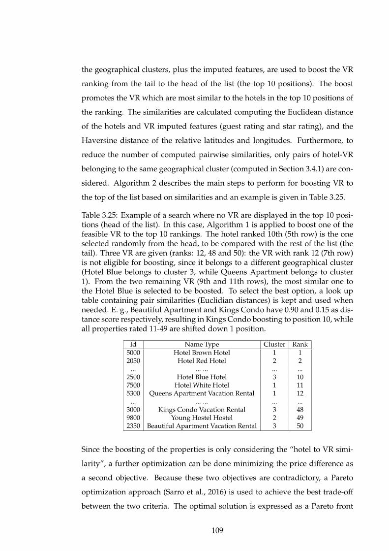
the geographical clusters, plus the imputed features, are used to boost the VR

ranking from the tail to the head of the list (the top 10 positions). The boost

promotes the VR which are most similar to the hotels in the top 10 positions of

the ranking. The similarities are calculated computing the Euclidean distance

of the hotels and VR imputed features (guest rating and star rating), and the

Haversine distance of the relative latitudes and longitudes. Furthermore, to

reduce the number of computed pairwise similarities, only pairs of hotel-VR

belonging to the same geographical cluster (computed in Section 3.4.1) are con-

sidered. Algorithm 2 describes the main steps to perform for boosting VR to

the top of the list based on similarities and an example is given in Table 3.25.

Table 3.25: Example of a search where no VR are displayed in the top 10 posi-tions (head of the list). In this case, Algorithm 1 is applied to boost one of thefeasible VR to the top 10 rankings. The hotel ranked 10th (5th row) is the oneselected randomly from the head, to be compared with the rest of the list (thetail). Three VR are given (ranks: 12, 48 and 50): the VR with rank 12 (7th row)is not eligible for boosting, since it belongs to a different geographical cluster(Hotel Blue belongs to cluster 3, while Queens Apartment belongs to cluster1). From the two remaining VR (9th and 11th rows), the most similar one tothe Hotel Blue is selected to be boosted. To select the best option, a look uptable containing pair similarities (Euclidian distances) is kept and used whenneeded. E. g., Beautiful Apartment and Kings Condo have 0.90 and 0.15 as dis-tance score respectively, resulting in Kings Condo boosting to position 10, whileall properties rated 11-49 are shifted down 1 position.

Id Name Type Cluster Rank5000 Hotel Brown Hotel 1 12050 Hotel Red Hotel 2 2

... ... ... ... ...2500 Hotel Blue Hotel 3 107500 Hotel White Hotel 1 115300 Queens Apartment Vacation Rental 1 12

... ... ... ... ...3000 Kings Condo Vacation Rental 3 489800 Young Hostel Hostel 2 492350 Beautiful Apartment Vacation Rental 3 50

Since the boosting of the properties is only considering the “hotel to VR simi-

larity”, a further optimization can be done minimizing the price difference as

a second objective. Because these two objectives are contradictory, a Pareto

optimization approach (Sarro et al., 2016) is used to achieve the best trade-off

between the two criteria. The optimal solution is expressed as a Pareto front

109

Algorithm 2 VR Boosting.1: procedure BOOSTVR2: Rank the properties with the RS;3: Select property i from the top 10 rankings with property type != “Vacation

Rental”;4: for X (properties ranked > 10) do:5: Select only the properties with property type = “Vacation Rental” (X0);6: From X0 select only the properties in the same geographical cluster

of i (X00);7: for each pair (i, j) with j 2 X00

do:8: Calculate sim(i, j) based on guest rating, star rating, latitude and

longitude;9: Select the most similar property j to i;

10: Replace i with j;

(Figure 3.13) representing non-dominated points of hotel-VR pairs (for which

no objective can be improved without worsening the other). In a formal way,

point x Pareto dominates point y iff the following two conditions hold:

fi(x) 6 fi(y)8i 2 {1, 2, ...,M} , (34)

fi(x) < fi(y) for at least one objective j 2 1, 2, ...,M, (35)

where the number of objectives M = 2 in this case. Solution x is called Pareto

optimal if there is no other solution z which Pareto dominates it (Figure 3.13).

The collection of all Pareto optimal solutions is called the Pareto optimal set,

and the Pareto optimal front is the projection of these solutions in the objective

space (Zhai and Jiang, 2015; Yuan et al., 2016; Rostami and Neri, 2017; Miranda

and Von Zuben, 2017).

Regarding the evaluation of the results for the imputation of guest rating and

star rating, the MAE is used as error function as it is of easier interpretability, re-

flecting on average how many error stars there are between the observed value

and the predicted one (e.g., MAE = 0.5 means an average error of a half star).

As recommended by Chen et al. (2009), I use MAP@X metric to compare the

ranking lists (with X = 1 and X = 5).

110

Figure 3.13: Pareto front example for one search. The dots represent non-dominated Pareto solutions in the similarity (y-axis) and difference in price(x-axis) objectives respectively.

A k-fold cross validation is applied splitting the dataset into independent train-

ing, validation and test subsets. The test set is generated using a uniform sam-

pling without repetitions, and the rest of the data is left as a training and vali-

dation sets. Furthermore, the ML-Spark pipelines (Meng et al., 2016) are used

to ensure correctness and replicability of the experiments. In machine learning,

the concept of pipeline (or workflow) is very important to guarantee that the

same set of steps are involved when a new dataset is processed. Figure 3.14

shows a pipeline in ML-Spark from the pre-processing to the regression phase.

The ML-Spark library represents such workflow as a sequence of steps to be

performed in a specific order. Due to the laziness of Spark transformations, the

pipeline is created as a recipe, stored in the memory and the computation is de-

ferred to the point where the fit(·) method is invoked (see Section 2.3.2 for more

details).

3.4.4 Results

As mentioned earlier, the co-clicks is an item-item measure which takes into

account the properties co-clicked by the user in a specific time frame. Let us

assume that in a year, a group of 1 million users are navigating through the

London properties catalogue. Every time a user clicks on multiple items dur-

ing the search, the number counting the co-clicked pairs increases by one. All

111

Figure 3.14: Workflow for a machine learning pipeline on ML-Spark. The topflow shows the abstract steps that are performed on the data. The bottom rep-resents the transformation applied to the data when the fit(·) method is invokedon a dataframe.

the values are scaled within [0, 1] range for estimating the similarity. The main

problem of this similarity measure, based on implicit feedback from the user,

is that for each new item added to the catalogue, there is no historical data

available, resulting in 0 similarity with all other items. The first objective of this

research is to find an approximation function (based on non-historical features),

which can be used as a proxy of the co-clicks (when they are not available). To

achieve this, two sets of engineered features based on amenities and geographi-

cal position are investigated. I carried out two experiments using the amenities:

the first one implements the Jaccard similarity metric (Niwattanakul et al., 2013;

Park and Kim, 2017) and the second one - the Weighted Hamming distance. The

Jaccard similarity (within [0, 1] interval, where 0 means completely dissimilar

and 1 represents identical), is defined in Eq. 3 where fi and fj are the two sets

of amenities related to properties i and j. The Jaccard similarity only considers

the number of shared amenities, without giving any preference to the amenity

popularity. On the other hand, the Weighted Hamming distance (within [0, inf]

range, when used as similarity measure a lower value means more similar)

takes into account the number of properties in which the amenity is available

(Eq. 4), where W is the amenity weight vector. Each element of W is calculated

as Inverse Document Frequency (IDF):

wk = idf(k,D) = log(N

|d 2 D : k 2 d|) , (36)

112

with D representing all amenity sets, N the total number of items (properties),

and |d 2 D : k 2 d| the number of properties in which the amenity k is available.

For the geographical features, a Fuzzy-C-Means (Pal et al., 2005; Koohi and

Kiani, 2016; Farokhi et al., 2016) (or soft clustering) algorithm is implemented

to group the properties and subsequently the Euclidean distance of their mem-

bership functions is used to calculate their similarities. To cluster the properties,

a three stage Spark pipeline is built: vectorization; standardization; and clus-

tering. The vectorization transforms a dataframe with one column per feature

in a one column dataframe containing a vector of features. The 0-mean and

unit-variance standardization is then applied to each feature in the vector and

the clustering groups the properties, based on a given parameter c (number of

clusters). The choice of c is empirically tested with values between 5 and 100,

with incremental step of 5. The final choice resulted in c = 10 for two main rea-

sons: the MAP@X accuracy was not significantly improving for values greater

than 10; and the clusters were meaningful (e.g., properties in the city centre all

in the same cluster, or near commute connections all in another cluster, etc).

While the Jaccard and Weighted Hamming are metrics able to measure the sim-

ilarity between two properties based on the quantity (the former) and quality

(the latter) of shared amenities, the Fuzzy-C-Means is solely depending on the

geographical characteristics, calculated using the latitude, longitude and their

derived geo-features (given in Section 3.4.1). For the co-clicks similarity pre-

diction, the MAP@x (x = 5) is used as accuracy measure. Table 3.26 shows the

probabilities of ranking property pairs with the three-similarity metrics against

the co-clicks ranking property at first place and in the top five positions. In

particular, the second column of the table gives the probability of a property

being ranked first by the co-clicks to be also ranked at the top by the other three

metrics, while the third column illustrates the probability when comparing the

first five positions of the rankings. In other words, column three show the accu-

racy of the Jaccard similarity, Weighted Hamming distance and Fuzzy-C-Means

rankings against the co-clicks similarity with rank from 1 to 5 (the first five are

chosen because they appear at the top of the screen). As can be seen from Ta-

ble 3.26, the accuracy when using the amenities as similarity measure is very

113

low (11% and 25% for the Jaccard similarity and 9% and 22% for the Weighted

Hamming distance respectively). The poor results can be explained by the cor-

relation between the co-clicks and the position of the properties in the raking

(two closely ranked items would have higher probability of being co-clicked

in the same session), while the amenities similarity (either Jaccard or Weighted

Hamming distance) only correlates properties based on the number and type

of matching amenities. For the Fuzzy-C-Means ranking, the achieved accuracy

is much higher (35% and 60% for the two ranking groups respectively) and this

could be related to the fact that usually the listed properties are geographically

close (in each search session the shown properties are from the queried destina-

tion). While the co-clicks still give a better insight of the properties similarity,

implicitly reflecting the users behaviour and choice; the geographical cluster-

ing offers a good approximation with a 35% of correctly ranked items in first

position (rank = 1), and 60% in the top 5 rankings, when the co-clicks similarity

information is missing (due to the lack of historical data for the new properties).

Table 3.26: MAP@5 accuracy scored by the three proposed similarity measurescompared only with the pairs of properties with co-clicks rank 2 [1,5]. The sec-ond column shows the probability of a property ranked first by the co-clickssimilarity, to be ranked in the first 5 positions by the other similarity metrics.The third column shows the accuracy of a property ranked in the first 5 posi-tions by the co-clicks similarity and all the other similarity metrics.

Method co-clicks rank = 1 co-clicks 16 rank 6 5Jaccard similarity ranking 0.11 0.25Weighted Hamming distance ranking 0.09 0.22Fuzzy-C-Means ranking 0.35 0.60

Two of the most frequently used features when selecting a property from a cata-

logue are the users rating and the quality of the property (e.g., star rating). Very

often this information is missing when a new item is added to the website and

both the RS and the user are most likely to underestimate its potential. To pro-

vide fairer ranking (as a second objective of this research), the two ratings are

imputed using available non-historical features (e.g., amenities and geographi-

cal position). From the initial dataset, I took out all the instances with missing

114

guest or star rating, which resulted in a complete subset (with no missing val-

ues). This set was then further split into 70% training and 30% testing subsets

respectively. Subsequently, missingness is introduced artificially in the guest

and star ratings, producing an incomplete testing set - used for the assessment

of imputation methods performance. Two baselines (mean and median impu-

tation) and the three state-of-the-art approaches for missing data imputation

are applied: K-Nearest neighbours Imputation (KNNI), Random Forests Impu-

tation (RFI) and Gradient Boosted Trees Regression (GBTI). All methods are de-

scribed in the background section and are here implemented using the Apache

Spark framework.

For the KNNI a value of K = 10 is used as suggested in (Batista and Monard,

2002). The main disadvantage of this method when applied to big data is the

low scalability due to O(N2) comparison needed and its questionable robust-

ness of the results (e.g., compared to ensemble methods). Both RFRI and GBTI

used in this work minimise the MAE function and use a 10% validation set to

avoid overfitting. The ML-Spark library implementation is used for both tree

models.

Firstly, the two baselines are used to calculate the mean (median) of the guest

rating (star rating) on the training set and substitute it in the test set. Secondly,

the model based imputation approaches are used. For each instance of the test

set (all with missing ratings), KNNI is used to calculate the ten most similar

neighbours from the training set, minimizing the Euclidean distance on the

weighted amenities and geographical features. The imputed value then is the

average of these ten guest and star ratings. For the RFI and GBTI, a four stage

Spark pipeline is set up to ensure replicable experiments: vectorization, stan-

dardization, cross validation, and regression. The cross-validation step splits

the complete dataset into a set of folds which are used as a training and valida-

tion subsets. E.g., with 10 folds, the cross validator generates 10 (training, vali-

dation) dataset pairs, each of which uses 9/10 of the data for training and 1/10

for validation iterating through them during the training phase. The regression

step involves the two algorithms described in Section 2.1 (i.e., RFRI and GBTI).

115

Table 3.27 contains results from applying the above imputation techniques on

guest and star ratings. As expected, the two baselines (mean and median im-

putation) achieved the lowest accuracy with MAE of 1.21 and 1.01 for the guest

rating, and 0.70 and 0.75 for star rating. From the implemented state-of-the-art

algorithms, KNNI produced the worst accuracy (0.70 and 0.50 for star and guest

rating respectively). This approach also appeared to be very slow, because of

the large number of samples in the training set (about 200K samples). The GBTI

technique with standardized features achieved the best result (0.36 for star rat-

ing and 0.34 for guest rating), followed by the RFI with the same setup (0.39

and 0.47 for star and guest rating respectively). The same experiments were

repeated removing the amenities from the dataset to assess the importance of

this feature. While the use of amenities as a feature failed the prediction of the

co-clicks similarity (Table 3.26), their use in the ratings imputation improved

the overall accuracy (Table 3.27). These contradictory results can be explained

by the fact that the amenities partially define the quality of the property (e.g., a

property with amenities such as pool and spa has higher likelihood to be rated

as a 5 star). On the other hand, the geographical position seems to be useful

for determining the guest rating (e.g., properties close to stations, airports or

famous landmarks have greater probability of receiving a higher rating).

Table 3.27: Guest rating and star rating imputation errors. The MAE is usedas error function to compare the imputation results of two baselines (meanand median imputation) and three state-of-the-art approaches (KNNI, RFI, andGBTI). The experiments are performed with (v) or without (-) amenities andstandardisation.

Method Amenities Standardization Guest Rating Star RatingMAE SD MAE SD

Mean v - 1.21 1.17 0.70 0.65Median v - 1.01 0.99 0.75 0.71KNNI v - 0.70 0.66 0.50 0.45

RFIv - 0.40 0.37 0.42 0.40- - 0.44 0.40 0.50 0.46v v 0.39 0.35 0.47 0.44

GBTIv - 0.37 0.34 0.39 0.36- - 0.40 0.37 0.44 0.42v v 0.34 0.31 0.36 0.33

116

Here I combine the geographical features, amenities and imputed guest and

star ratings to re-rank the properties in two million searches collected in one

month (Table 3.28) using Algorithm 2.

The third row of the table shows 65% searches without VR in the top 10 rank-

ings (35% of the searches already contain at least one VR in the top 10, so they

are not affected by the algorithm). From the 65% searches, only those with

VR ranked higher than 10 (rank > 10) are considered, resulting in total eligible

searches of 31% (row 4). Subsequently, from the 31% of searches, the feasible

VR are subject to three main rules: do not boost VR too far from the paired hotel

(row 5); do not boost VR which is not similar enough to its paired hotel (row

6); and only consider hotels ranked in positions 5 to 10 for the pairs (row 7).

Following these rules brings the number of eligible searches (row 8) to 291705

(13%), with 1801023 (the number of hotel-VR pairs that satisfy the distance and

similarity metrics) possible boosts (6 possible boosts per each search on aver-

age).

Table 3.28: Offline experimentation on one month of real world searches. Thetotal number of searches and the eligible searches for a boost after applyingdifferent filters are shown. The last two rows give the total number of possibleboosts and the number.

Types of searches #Searches %SearchesTotal searches 2206479 100Without VR in top 10 1446976 65VR with rank > 10 697418 31Searches with eligible VRwithin chosen distance

324289 14

Searches with eligible VRwithin chosen distance, and sim < ↵ (0.05)

316977 14

Searches with eligible VRwithin chosen distance, sim < ↵ (0.05)and hotels ranked between 5 and 10

291705 13

Types of boosts #Boosts %BoostsTotal number of possible boosts 1801023 100Total number of optimal boosts (in the Pareto front) 449070 25

At this point the Pareto optimization using the two objectives (pair similarity

and pair price difference) is applied considering only non-dominated solutions.

This approach reduced the number of possible boosts by 75% (1.54 possible

boosts per search on average), excluding all dominated Pareto solutions. The

selection of similarity threshold (row 6 of Table 3.28), beside the use of human

117

expertise, can be done applying statistical test to ensure that the similarity and

price difference are statically significant (p-value < 0.05) (the difference is small

enough to consider a boost). To do so, all the points from each Pareto front

are standardized with 0-mean and unit-variance. From the set of standardized

points, I consider only those with std < 2 (assuming normal distribution, this

corresponds to the 95st percentile). Figure 3.15 shows the standardized Pareto

front for a one-day searches. All solutions with std > 2 are not considered.

A statistical t-test is finally used to compare the distribution of the features in

the top 10 ranks (e.g., guest rating, star rating, price, distance from city centre,

distance from airports, etc). The t-test showed that the boosting of one Pareto

optimal VR in each search doesn’t statistically change these distributions (p-

value < 0.05). The same t-test repeated when boosting dominated Pareto VR

solutions, showed statistical changes in the features’ distribution of the top 10

ranks (p-value > 0.05). This results leads to the conclusion that the sub-optimal

VR solutions are not recommended during the boosting phase due to the statis-

tically different features from those of the compared hotels.

Figure 3.15: All Pareto front solutions standardized with 0-mean and unit-variance. Only the solutions with std 6 2 are used for the boost (all hexagonsin the (2, 2) square). This plot illustrates a sample of only one-day searches(about 70000). The x and y axes represent the difference in price and propertysimilarity respectively.

118

3.4.5 Discussion

The missing data problem for travel Recommender Systems is investigated giv-

ing focus on the VR market. After an initial exploratory analysis, the dataset of

properties at hand showed 50% and 19% missingness for guest rating and star

rating respectively. Furthermore, the properties similarity, namely the co-clicks,

is always missing when a new property is added in the catalogue (because there

is no historical data of users co-clicks with other properties). To deal with that,

non-historical features (amenities and geographical position) are introduced,

analysed and used to determine the best proxy of the co-clicks (when not avail-

able). Results from the applied three similarity measures (Jaccard, Weighted

Hamming and Fuzzy-C-Means rankings) showed the Fuzzy-C-Means to be the

best approximation metric with 35% of correctly ranked items in first position,

and 60% for the top 5 rankings, indicating a correlation between the co-clicked

properties and their position on the map. The applied data imputation tech-

niques for mitigating the guest and star ratings missingness (two baselines:

mean and median imputation; and three state-of-the-art models: KNNI, RFI,

and GBTI), resulted in recommending the GBTI as the most suitable one for

this task, achieving the lowest MAE (0.36 and 0.34 for guest and star rating re-

spectively), followed by the RFI and KNNI. As expected, the baselines scored

the lowest accuracy, with an error greater than 1 for guest rating and 0.75 for the

star rating (both ranging one to five). Furthermore, the importance of amenities

as a feature for this task is assessed repeating the same experiment using only

the geographical features. While the use of amenities failed the prediction of

the co-clicks similarity (with an accuracy between 9% and 25%), their use in the

ratings imputation always improved the overall accuracy. Lastly, the VR long

tail is considered as a multi-objective problem, optimising the hotel-VR similar-

ity and their difference in price as the two objectives. From an initial 2 million

considered searches, only 35% had at least one VR in the top 10 rankings, while

after the Pareto optimization, the percentage increased to 48%. Furthermore,

the boost of optimal solutions (non-dominated) does not change the distribu-

tions of the features in the head of the list. Future work would analyse the

119

behaviour of the RS when the engineered and imputed features are used dur-

ing the recommendation process for the VR properties. In addition to that, new

error functions will be tested to assess and distinguish the current under/over

estimation of the imputed ratings by the model based techniques.

3.5 Large Scale Missing Data Imputation

When Big Data is considered, the problem of the missing data imputation is

still of primary importance for the successful implementation of machine learn-

ing techniques (e.g., recommendation tasks where millions of users and thou-

sands of items are involved). Usually, the probability of having missing data

increases with the number of features in the dataset and with the number of

samples, making the imputation task in big data context extremely important.

However, if the missing entries are few compared to the scale of the dataset, a

deletion method is applicable without losing statistical strength. On the other

hand, if the number of missing values grows with the size of the dataset the

imputation is necessary to preserve, or even increase, the statistical power of

the data (or in general to not lose too many samples during the pre-processing

stage). Unfortunately, almost all the imputation techniques proposed in liter-

ature (Musil et al., 2002; Schmitt et al., 2015; Petrozziello and Jordanov, 2017a,

2018) require the whole dataset to be provided for the model at imputation time,

which means that adequate memory allocation is needed, making the task un-

feasible for datasets composed of hundreds of features and millions of samples.

Not many methods have been proposed to cope with the missing data problem

in the big data field (Anagnostopoulos and Triantafillou, 2014) due to the in-

herent complexity of the task (both related to time and memory constraints).

Neural Networks are state of the art machine learning approach for several

different domains with recent advances in image processing (Sun et al., 2013),

pattern and speech recognition (Deng et al., 2013), that involve fitting of large

architectures (with thousands of weights) to large datasets (several gigabytes to

few terabytes). Given the scale of these machine learning problems, training can

take up to days or even weeks on a single machine using the commonly applied

120

optimization techniques (e.g., stochastic gradient descent (SGD)) (Bottou, 2010).

For this reason, research focussed on the distribution of machine learning algo-

rithms across multiple machines. Different attempts have been made to speed

up the training of NN using asynchronous jobs (Chilimbi et al., 2014). In the

parameter server model (Li et al., 2014), one master holds the latest model pa-

rameters in memory, serving the workers nodes on request. The nodes compute

the gradient on a mini batch drawn from the local hard drive. The gradients

are then shipped back to the server, which updates the model parameters. With

the introduction of the Map-Reduce paradigm, different frameworks emerged

to leverage resources of a cluster (e.g., Apache Hadoop and Apache Spark).

Here, I propose a Distributed Neural Network Imputation (D-NNI) framework

(Figure 3.16), leveraging the idea of mini-batch training in a distributed fashion

over Spark to reduce training time, while making at the same time the imputa-

tion of new values possible even for larger datasets. The proposed imputation

approach (Petrozziello et al., 2018b) is tested on a real-world dataset composed

of 400K samples (Petrozziello and Jordanov, 2017b), and 645 features (of which

57 including missing values).

Figure 3.16: Distributed Neural Network architecture in Spark (Section 3.5.1).

3.5.1 A distributed Neural Network architecture on Spark

The implementation of the imputation stage through distributed neural net-

works builds on Apache Spark and the open source Neuron library (Unknown,

2017) (a lightweight Neural Network library written in Scala providing all the

121

Table 3.29: Neural Network Trait.

building blocks (e.g., layers, optimizers, back-propagation, etc.), to create our

own distributed version (Table 3.29 shows the Neural Network Scala interface).

By building on top of Spark, I utilise the advantages of modern batch com-

putational frameworks, which includes: the high-throughput loading and pre-

processing of data; and the ability to keep data in memory between operations.

Furthermore, the implementation of the D-NNI as a Spark pipeline stage allows

the imputation to be easily included as a pre-processing stage of any dataset.

Table 3.30 and Table 3.31 show code snippets of how the imputation stage is

created. In particular, Table 3.30 presents how the layout of the network is de-

fined (using a sequence of layers, with the initial one representing the input,

and the last one the output (which can be as large as the number of imputed

features)), while Table 3.31 demonstrates the creation of a Spark pipeline impu-

tation stage. The NeuralNetworkImputationStage object exposes several methods

to: set the input columns (i.e., the features used during the learning phase); the

target columns (the ones containing missing values); the predicted columns (the

stage returns a new dataframe containing additional columns with the imputed

values); and the additional parameters used during the imputation procedure

(i.e., the NN layout as defined in Table 3.30, the optimizer hyper-parameters,

the weights initialization procedure, the loss function, etc).

In this work I use a data-parallelization schema with synchronization and a

122

Table 3.30: Example of network specification for D-NNI.

Table 3.31: Create a Missing Imputation Stage in a Spark pipeline, the fit(·)method is used to train the imputation model, once the model is trained(i.e., imputationModel object), the missing values can be imputed using thetransform(·) method of the model.

central coordinator, labelled naive parallelization by Moritz et al. (2015). In

every iteration, each worker node c in the cluster C computes a local gradient

gc for a batch of data bc, then these vectors are (tree-) aggregated,

g =1C

X

c

gc(bc) , (37)

and sent back to the master which performs the SGD update step and broad-

casts the new weights (W) to all c 2 C (Figure 3.16). In the absence of network

overhead and aggregation cost this setup scales linearly with the number of

worker nodes. Under more realistic conditions, the optimal number of nodes

depends on the size of bw and the network overhead.

123

Table 3.32: Sample of the dataset containing the features used for the proper-ties recommendation. Missing values (values that are not available for a shorthistory) are denoted with a “-”.


To test the proposed technique I partially re-use the dataset of Section 3.4.1. In

addition to the already seen amenities, properties and destinations tables, I also

included a dataset of historical prices displayed on the website, calculated us-

ing three different time spans: a 1-day; a 3-day; and a 7-day average. This

additional information is joined to the others on the property ID to have all

needed information for a each specific property. A subset of features of this fi-

nal dataset is showed in Table 3.32, while a summary of the features contained

in each dataset is given in Table 3.33.

The proposal is compared with two baselines (mean and mdian imputation

by market) and two state-of-the-art techniques (Linear Regression Imputation

(LRI) and K-Nearest Neighbour Imputation (KNNI) which are easy to distribute

and already available in the Apache Spark framework (also described in Sec-

tion 2.1), while the results are assessed on the R2 coefficient (Eq. 18) as both

RMSE and MAE are scale dependent and therefore of hard comparability across

a large set of features.

Table 3.33: Summary of the features used in the OTAs dataset.

124

0

20

40

60

2003

2004

2005

2006

2007

2008

2009

2010

2011

2012

2013

2014

2015

2016

2017

year

Log(growth)

Figure 3.17: Log growth of the properties in the catalogue (black line) and loggrowth of missing data (red line).

3.5.3 Results and discussion

The empirical experiment on the RS for OTA dataset is carried to test the im-

putation accuracy and time feasibility of the proposed technique. Before the

imputation, the data is split into a training set (70%) and a test set (30%). The

investigated NN topology includes two hidden layers (n-n-n-k), with n being

the number of inputs (n = 657) and k the number of outputs (k = 57). After each

hidden layer, a ReLU activation function is used to transform the data (a ReLU

is also applied in the output layer as all the missing values belong to features in

R>0. The training set is further divided into 80% for training and 20% for vali-

dation, and the R2 coefficient is used to evaluate the learning performance. The

stopping condition includes 2000 training epochs, gradient reaching value less

than 1.0E-06, or 6 consequent failed validation checks, whichever occurs first.

Figure 3.18 shows the R2 metric across the 57 considered features. As can be

seen, the D-NNI outperforms the other techniques (larger R2 value) for many

of the imputed features. The range of R2 for the D-NNI spans from 0.07 to

0.95 with a median of 0.56. The second best method (LRI) has its lowest impu-

tation performance at 0 (same as all the other compared techniques), the best

125

Figure 3.18: Boxplot for the R2 measure on the 57 imputed variables.

at 0.87 and a median R2 of 0.38. Following are the mean imputation, KNNI

and median imputation with 0.27, 0.26 and 0.18 median R2 respectively. It is

also worth to notice that the mean and median imputation techniques have a

few outliers reaching an R2 above 0.80, this is happening with features skewed

toward one value (low variance), hence closer to the mean (median) of the im-

puted one. The R2 for each feature with missing values is also presented in

Figure 3.19. As can be seen, the prediction accuracy of the D-NNI is always

greater of those provided by the LRI and KNNI. For the mean (median) impu-

tation, the D-NNI is better in 51 out of 57 cases, while still being comparable in

the six remaining features (i.e., pct gt ly amer posa h, pct gt ly emea posa h,

etc. (see Figure 3.19). Figure 3.20 shows one of the best (i.e., gt ly h) and worst

(i.e., pct gt stay month 4 h) imputed features for the D-NNI, illustrating the

NN ability to predict with high accuracy continuous features (Figure 3.20a),

while struggling with the zero inflated ones (Figure 3.20b) (but still achieving

better imputation accuracy compared to the other models).

Furthermore, in Table 3.34 the running times over 10 runs for the five imputa-

tion techniques are displayed when using the following Amazon Web Service

cloud cluster configuration: Master (r4.xlarge, 30gb, 4 cores) and 8 Workers

(15gb, 8 cores). The average and standard deviation in minutes are reported,

showing the D-NNI as the slowest method to impute, with a large variance

across different runs (depending on the convergence speed for the training

phase). The second slowest method is the LRI. Here, the 57 features contain-

126

Figure 3.19: Boxplot for the R2 measure on the 57 imputed variables.

ing missing values are independently fitted, reason for the achieved imputation

speed. It would be expected a linear decrease in speed using up to 57 workers

(where each node of the cluster is fitting a different feature). The fastest impu-

tation models appeared to be the mean (median) imputation, where the predic-

tion only finds the average (median) of each feature with missing values. The

KNNI speed is not reported as the imputation was not possible with the consid-

ered cluster configuration (not enough memory to fit the N2 pair matrix). When

increasing the cluster size to 20 nodes, the KNNI imputation took 40 minutes,

with a standard deviation of 8 minutes, mainly due to communication latency

among the workers.

Table 3.34: Average and std run time (in minutes) over 10 runs.

Table 3.35: Speedup ratio of the NN compared to the sequential model, fornumber of samples in batch (10% to 70%) against number of workers (2 to 8).

To measure the D-NNI sensitivity to the batch size and the number of workers,

I consider a grid of values from 10 to 70 for the first parameter, and 2 to 8 for

the second one. For each training run I compute the achieved speedup (Eq. 26)

127

(a) (b)

Figure 3.20: Predicted (x-axis) and observed (y-axis) values for the D-NNI. Fig-ure 3.20a (left) shows the historical yearly gross transactions of each property,while Figure 3.20b (right) depicts the yearly percentage transactions for onemonth (April).

relative to training on a single node (sequential NN with SGD). In Table 3.35

the imputation speedup for the D-NNI model under 21 different settings is re-

ported. Table 3.35 exhibits several trends, with the top row representing the

case of two machines. As can be seen, the speedup decreases when increment-

ing the batch size, which is due to the training taking the largest part of the

total computational time, while the communication between nodes is negligi-

ble. The same trend still holds in the case of 4 machines (2nd row). In the 3rd

row, the trend shows reduction of the speedup up to the batch size of 50%. The

subsequent increase of the ratio (for 60% and 70%) could be due to the time

being evenly split between training and communication, and from randomness

due to fluctuation in the convergence of the optimization process.

Another interesting trend can be observed when inspecting the table by columns.

Is true almost for all cases that the use of 4 nodes gives the best speedup over 2

and 8. This could be explained by the quantity of data used for training. When

a certain threshold for the number of workers is passed, the overhead for com-

munication and synchronization can become larger than the actual processing

time. This is enforced by the fact that the trend is less accentuated when mov-

ing toward bigger batches. For 40% and 50%, the speedup for 4 and 8 nodes

128

is almost identical, while for 8 nodes the speedup is higher when using more

than 50% of data in each batch.

3.6 Conclusion

Here, the missing data problem affecting machine learning tasks has been in-

vestigated. This chapter explored a variety of use cases where the effective

imputation of missing values can benefit the learning process. An extensive

search through related works in missing data imputation allowed to identify

a series of gaps which have been tackled and different novel solutions have

been proposed. The main proposals are: the analysis of the impact of missing

data on the radar classification task in both the binary and multi-class settings;

the “Scattered Feature Guided Data Imputation” which focuses on finding the

best performing imputation algorithm for each feature of a dataset through a

learning procedure; the study of the impact of missing data in Recommender

Systems and the proposal of a bi-objective Pareto front algorithm to boost un-

fairly ranked properties after imputation of their missing values; and the “Dis-

tributed Neural Network Imputation” which allows to impute missing data at

scale (datasets not fitting on one machine) through the use of the Spark frame-

work and a cluster of machines.

129

4 Deep Learning Methods for Real-World Problems

In this chapter I investigate the use of Deep Learning approaches applied to

three real-world problems. In the first one, I use both Convolutional Neural

Networks and Long Short Term Memory Networks for the detection of hypoxia

during labour. Those models are compared with current clinical practice and

computerized approaches and a new architecture, namely Multimodal Con-

volutional Neural Network is proposed Petrozziello et al. (2018a, 2019). The

second part of this chapter explores the profitability of Multivariate Long Short

Term Memory Networks for the forecast of stock market volatility. The method

is compared with univariate and multivariate Recurrent Neural Networks, as

well as with state of the art univariate techniques from the financial field. Lastly,

Convolutional Neural Networks and Stacked Autoencoders are used to detect

threats from hand-luggage and courier parcel x-ray images (Petrozziello and

Jordanov, 2019).

4.1 Deep Learning for fetal monitoring in labour

During labour, materno-fetal respiratory exchange is transiently compromised

by uterine contractions leading to reduced oxygen supply to the foetus. The foe-

tus responds by adjusting its cardiac output, redistributing blood to prioritise

the heart and brain, and adapting metabolically. Failure of fetal compensation

leads to brain injury or death. The cardiotocogram (CTG, Figure 4.1) contin-

uously displays the fetal heart rate and uterine contractions on a paper strip.

This is examined visually in real time to detect the foetus that may benefit from

emergency operative delivery (Caesarean or instrumental vaginal birth). The

CTG is exceptionally complex, showing patterns that variably reflect periodic

changes in fetal sleep state, responses to the stresses of uterine contractions, re-

sponses to maternal position, anaesthesia, pregnancy complications, infection,

stage of labour, in addition to features that reflect terminal decompensation.

Hence, fetal assessment in labour is challenging and progressed little in the

past 45 years (Timmins and Clark, 2015). In the developed world, the long

130

Figure 4.1: Cardiotocogram (CTG) in labour (a 30min snippet).

time series of the CTG are still assessed by eye (Figure 4.1). In the UK, during

labour at term, about 100 healthy babies die and about 1100 sustain brain in-

jury (Kurinczuk et al., 2010; Walsh et al., 2008). Nearly 50% of the total NHS

litigation bill is due to obstetric claims (3.1bn in 2000-2010), the majority relat-

ing to shortcomings in labour management and cardiotography interpretation

(Figure 4.1) (Authority, 2012). Each neonatal death or permanent brain dam-

age is devastating for the family. The cost of insurance against litigation per

birth in the UK is 20% of the total delivery cost (Davies, 2015). At the same

time, around 100 unnecessary emergency deliveries are performed each day in

the UK alone, with major financial and potentially life-long consequences, such

as increased risks of uterine rupture and/or stillbirth in next pregnancies, ma-

ternal incontinence, and post-traumatic stress disorder (unpublished estimate

based on the database provided by Oxford, UK). Worldwide, about 2.6 million

stillbirths occurred in 2015. Intrapartum stillbirths predominantly occur in low

resource settings and overall are considered to be mostly preventable by CTG

monitoring in labour (Lawn et al., 2016), which is largely not available in the

developing world. However, due to its high false positive rate, even in the

developed world, CTG is often not offered in labours considered to be low-risk.

The work presented here arises from prior work with the Oxford digital archive

of 59279 term deliveries: a uniquely large birth cohort spanning nearly 20 years

and growing daily. Georgieva et al. (2017) have already developed a basic pro-

totype diagnostic system (OxSys 1.5) that objectively quantifies the CTG in the

131

context of clinical risk factors; and relates these to perinatal outcome. OxSys

1.5 already compares favourably to clinical assessment (on retrospective data),

with higher sensitivity for fetal compromise (37.6% vs. 32.2%, p < 0.05) and

lower intervention rate in normal outcomes, i.e. false positive rate (14.5% vs.

16.4%, p < 0.001). However, OxSys 1.5 employs only two diagnostic rules

based on feature extraction and clinical risk factors. The main CTG feature

used by OxSys 1.5 is the decelerative capacity (DC) of the phase rectified sig-

nal averaging (PRSA) algorithm - a combined measure of the frequency, depth,

and slope of any dips in the fetal heart rate (Georgieva, 2016; Georgieva et al.,

2017). The large size of the data archive confers scope for substantial improve-

ment. Deep Learning approaches have been successful with various real-world

problems at “learning” the most relevant unbiased and new information from

large datasets (LeCun et al., 2015). Hence, the aim is to apply Deep Learning

to interrogate the CTG archive and establish optimal ways to classify the CTG

into high and low risk.

In Section 4.1.5 (point 2) I report results of my pilot simulations and experi-

ments of applying Long Short Term Memory (LSTM) and Convolutional Neu-

ral Networks (CNN) to CTG assessment: I analyse the CTGs from 35429 labours

(85% were used for training with cross validation and 15% were set aside for

testing). I demonstrate that increasing the training set size and considering in-

formation about the quality of the contraction signal improved the performance

of the classifier. However, I only focused on the last hour of CTG monitoring

without distinguishing or adapting to the stage of labour (an important clinical

confounder to CTG interpretation) or including information about signal loss

in the fetal heart rate signal. However, fetal heart rate signals are notorious for

their poor signal quality owing to signal loss; erroneous pick up of maternal

heart rate; signal noise or gaps in monitoring. Although both LSTM and CNN

demonstrated promising performance worthy of further developments, CNN

showed slightly superior results to LSTM. The LSTM is generally more suitable

for forecast tasks over classification ones, and it suffered from vanishing gradi-

ent problems during back-propagation when learning on the long CTG records.

132

On the other hand, CNN proved to work effectively with long temporal data

through the use of moving filters and max-pooling.

In Section 4.1.5 (points 3 and 4) I build on the pilot study and aim to improve my

initial application of CNNs to CTG interpretation by: developing Multimodal

CNN (MCNN) for CTG interpretation that allow the input of signal quality fea-

tures (in this work) and other inputs (out of the scope here); developing Stacked

MCNN to analyse separately the CTG before and after the onset of active push-

ing (first and second stage labour), while feeding the risk assessment from the

first stage model into the second stage model; assessing the impact of the fetal

heart rate signal quality on the models performance.

I also extend the range of the testing to a new external dataset: Signal Processing

and Monitoring (SPaM) Workshop 2017 challenge dataset.

4.1.1 Datasets

1) Oxford data

I analysed the data from all monitored labours at the John Radcliffe Hospital,

Oxford between 1993 and 2011 that met the following inclusion criteria:

• term delivery of a foetus at 36 weeks gestation or more;

• intrapartum (in-labour) CTG comprising fetal heart rate and contractions

(Figure 4.1), longer than 15minutes, ending within three hours of birth

(only high risk women are monitored in the UK - roughly 50% of births);

• validated cord gas analysis at the time of birth, indicating the adequacy of

fetal blood oxygenation. In practice the acidity of the blood, measured by

pH, is the most appropriate way of grading this problem and indicates an

increased risk for long term compromise of the baby. Cord gases are anal-

ysed at the discretion of the clinician - in about 65% of all continuously

monitored births in the Oxford unit.

Excluded are babies with breech presentation and congenital abnormalities.

There are four exclusive groups according to the outcome of labour:

• severe compromise (comprising one or more of any stillbirth, any neona-

133

tal death, seizures, resuscitation followed by > 48hrs in neonatal inten-

sive, regardless of the arterial cord pH);

• moderate compromise: arterial cord pH at birth below 7.05;

• intermediate arterial cord pH between 7.05 and 7.15: the status of the out-

come of an intermediate pH is uncertain. This is especially the case when

delivery has been expedited for concerns about fetal welfare, when more

severe problems could have occurred if the labour continued without in-

tervention. These outcomes are labelled as intermediate/uncertain.

• normal: arterial cord pH>7.15.

A low arterial cord pH (increased acid content) reflects the duration of reduced

fetal oxygenation at the time of birth. However, cases with severe compro-

mise often have normal cord pH values at birth (about 60% of cases). These

represent a heterogeneous group of pathologies in which the pathway to brain

injury in utero is not fully understood. Cases with low pH (with or without

severe compromise) represent a more homogeneous set indicating the fetal in-

jury occurred as a consequence of oxygen deficiency specifically during labour

and at birth. This is a group more likely to exhibit changes in the CTG to allow

detection/prediction. For this reason, and for consistency with the open ac-

cess datasets who define compromise as pH<7.05 (see below), I split the testing

set to parts A and B and report the results separately (but still training the net-

works using all the data). Test Set A comprises of all Normal cases (n=4249) and

all moderate compromises plus the severe compromises with cord pH<7.05

(n=180). Test Set B comprises of all intermediate/uncertain cases (n=845) and

all severe compromises with pH > 7.05 (n=40). This inclusion/exclusion cri-

teria results in 35429 births with CTG in labour and details about the labour

outcome. In these, the testing subset of CTGs were identified by a random se-

lection of 15% of cases within each outcome group, ensuring similar rates of

compromise in training and testing. Overall, there are 1796 (5%) traces shorter

than one hour where I coded the missing values with zeros. The CTG data is

originally available at 4Hz for the fetal heart rate and 1Hz for the uterine signal

(as default output from the monitors). Signal loss or noise in the heart rate sig-

134

nal is common and here basic pre-processing is applied before smoothing the

heart rate to 0.25Hz. Therefore, one hour of data corresponded to 900 heart rate

and 900 contraction signal samples.

2) External open access datasets

Data-driven CTG interpretation is a narrow field with only several teams world-

wide working on this clinical problem. In the past five years there has been

a strong will from a few teams to begin creating open access databases that

would allow comparison between different approaches, as well as providing

at least some data for others to use as training data. Currently, there are two

such datasets available and I tested the proposed algorithms on both: firstly, be-

cause routine data coming from other hospitals/countries would be inevitably

influenced by varying clinical practice and ability to perform emergency inter-

vention, providing therefore external validation; and secondly, because in the

future, I would hope practitioners could use the same open-access datasets to

test and compare new approaches.

The Signal Processing and Monitoring (SPaM) in Labour Workshop 2017 database

comprises 300 labours collected from three participating centres (Lyon, Brno

and Oxford). Each centre provided 100 cases: 80 with normal pH and 20 with

pH<7.05, i.e. it was selected specifically to have a higher than usual rate of

compromised cases (i.e. 20% which is five times higher than that in the Oxford

cohort). To avoid any contamination between the SPaM data coming from Ox-

ford and the Oxford training data, the proposed Deep Learning approaches are

only tested on the 200 SPaM cases coming from Lyon (France) and Brno (Czech

Republic).

The Czech Technical University / University Hospital Brno (CTU-UHB) com-

prises 552 cases of which 40 (7%) have cord acidemia at birth below 7.05 (more

details on the dataset are provided in (Chudacek et al., 2014)).

135

4.1.2 Proposed Deep Learning models

To tackle the problem of an unbalanced training dataset (4% compromised ba-

bies vs. 96% healthy ones), I adopt a weighted binary cross-entropy error func-

tion:

CE = -tlog(s)- (1 - t)log(1 - s) , (38)

where t1 and s1 are the ground-truth and the scores respectively.

The class weights is set such that one misclassification from the compromised

group contributes to the error as much as 24 misclassifications from the healthy

group (reflecting the incidence of 1 in 24 of compromised cases in the data). In

the pilot experimentation, I also tested down-sampling and bootstrapping tech-

niques to handle the imbalanced dataset in the training phase but with worse

generalization performance on unseen data.

1) Preliminary Convolutional Neural Networks (CNN) and Long Short Term Memory

Network (LSTM)

As a first experimentation, I implemented both CNN and LSTM models. The

proposed single channel CNN has one input layer with size 2x900 points, cor-

responding to one hour of fetal monitoring at 0.25Hz (fetal heart rate and con-

tractions). The network comprises five convolutional layers (with max-pooling

and ReLU activation function) Figure 4.2. The last max-pooling layer is flat-

tened and fed as input to a fully connected layer. The class probability is

then computed using a softmax activation function. Batch normalization and

dropout are used through the network (Wan et al., 2013). I assess the quality of

the CTG contraction signals by an established autoregressive model (Cazares

et al., 2001), imposing the following restriction: >40min of acceptable quality,

of which >20min is of excellent quality. To avoid overloading the network with

noise, only the uterine signals that met this condition is used in the networks

(24%), whereas the remainder are substituted with zero.

The implemented LSTM follows the model presented by Graves (2013). The

136

Figure 4.2: Convolutional Neural Network topology. FHR - fetal heart rate;CNN - convolutional neural network.

main advantage of this architecture is its ability to capture both long and short

time dependencies in time series, which have proven to be effective in many do-

mains (including medical applications) (Choi et al., 2016). The LSTM has two

inputs: fetal heart rate and contraction signals; and two outputs: healthy and

compromised newborns. The LSTM architecture includes hyperbolic tangent

as a hidden activation function and a hard sigmoid as a recurrent activation

(default activation functions for LSTM, as advised by Hochreiter and Schmid-

huber (1997)). To get a binary class probability, a softmax function is used in the

output layer (Figure 4.3). The data is normalized before being inputted in the

LSTM.

Figure 4.3: Long Short Term Memory Network topology. FHR - fetal heart rate;LSTM - Long Short Term Memory.

2) Multimodal Convolutional Neural Networks (MCNN)

Here I propose a Multimodal Convolutional Neural Network (MCNN), com-

137

prising different inputs layers and independent learning branches (Figure 4.4).

The MCNN allowed me to use a variety of input sources: fetal heart rate,

uterine contraction and a fetal heart rate quality score vector. The heart rate

and uterine signals are fed into two distinct 5-layer convolutional networks

branches, while the heart rate quality is used as a score multiplier of the heart

rate convolutional branch, giving a weight for each output (each quality score

is calculated on a 15 minutes window with 5 minutes overlap as per the default

OxSys pre-processing (Cazares et al., 2001)). In particular, the signal quality in

each 15min window is calculated using the raw 4Hz data as the ratio of valid

signal data points out of the total number of signal points in the window. As

is in the canonical CNN, the last layer uses a softmax transformation to get

the class probability of each sample. The convolutional layer hyper-parameters

(i.e., number of filters and filter length) are independently optimized for each

layer, granting more flexibility during the network creation. A Bayesian hyper-

parameters optimization with Gaussian Process (Bergstra et al., 2011) is used,

and its parameters and optimal values are reported in Section 4.1.5.

Figure 4.4: Multimodal Neural Convolutional Network topology. FHR - fetalheart rate; CNN - convolutional neural network.

3) Stacked MCNN

The ability of the network to correctly predict the labour outcome using data

from the end of the CTG, which may often coincide with imminent delivery, is

a relevant result from a classification perspective. But it is important to note

that, at this time, the alert may be too close to the delivery, not allowing enough

time for appropriate intervention. To address this problem, I split the time se-

138

ries into two parts, the first one being the last 60 minutes of 1st labour stage

(900 data points); and the second one being the last 30 minutes of 2nd labour

stage (450 data points). I only consider 30 minutes in the 2nd stage of labour

because significant physiological changes are expected in a shorter time span

and because often the second stage does not last longer than 30 min. As in

the pilot study, deliveries with less than 900 and 450 data points for 1st and 2nd

stage respectively, are zero padded at the front. In the Stacked MCNN, the class

probability from the MCNN applied to the 1st stage of labour is used as addi-

tional input into the MCNN analysing the 2nd stage of labour (Figure 4.5). The

Stacked MCNN is then tested and, if the baby is delivered by intervention in the

1st stage of labour and thus had no monitoring in the 2nd stage, the probability

of the first MCNN is considered as the relevant MCNNs outcome prediction for

this baby.

Figure 4.5: Stacked MCNN topology for 1st and 2nd stage classification. FHR -fetal heart rate. MCNN - multimodal convolutional neural network.

4.1.3 State of the art methods

1) Clinical practice

The primary reason for operative delivery (Caesarean, Forceps or Ventouse de-

livery) is noted in the patient records by the attending clinician at the time of

birth, when applicable. This information is used to define true and false posi-

tive rates as follows: TPR - the number of operative deliveries for presumed fetal

139

compromise where there is a compromise as a proportion of the total number of

compromises; FPR - the number of operative deliveries for presumed fetal com-

promise where there is no compromise as a proportion of the total number of

normal cases.

2) Phase Rectified Signal Averaging (PRSA), also known as Decelerative Capacity

(DC)

A signal processing method proposed by Bauer et al. (2006) for the analysis of

adult fetal heart rate variability. Successively adapted and optimized for fe-

tal heart rate monitoring in labour (Georgieva et al., 2014; Rivolta et al., 2014).

Here, the maximum PRSA (maxPRSA) value per CTG segment of interest (i.e.

60 or 30min corresponding to 10 or 4 15min windows respectively) is consid-

ered.

3) OxSys 1.5

A current prototype of the Oxford system for data-driven fetal monitoring in

labour (Georgieva et al., 2017). This is under development and newer versions

will be available with time. OxSys 1.5 uses only two fetal heart rate features

(DC and the number of accelerations). It also uses two clinical risk factors -

the presence/absence of thick meconium or pre-eclampsia. OxSys analyses the

entire fetal heart rate with a 15min sliding window (5min sliding step) and

produces an alert if the risk for the foetus is high.

4.1.4 Performance metrics

Each of the proposed models are trained following a 3-fold cross validation

schema to avoid overfitting. Five runs of each algorithm are performed to ad-

dress the neural networks randomness and the median performance metrics

for the five runs is reported. The networks is evaluated using standard perfor-

mance metrics for classification tasks, such as AUC-ROC, TPR and FPR. The

AUC-ROC is suitable for unbalanced datasets because it is not biased by the

size of each class. Results are reported for TPR with a fixed FPR of 5, 10, 15 and

20 percent, relating to the FPR in clinical practice of 16% - 21% (Georgieva et al.,

140

2017; Abry et al., 2018).

4.1.5 Results

1) Parameters Optimization

For all proposed models, I use Bayesian optimization with Gaussian Process, a

popular model for parameter optimization (Bergstra et al., 2011) to maximize

the models’ TPR at 15% FPR. A high FPR is one of the most important defects

of CTG analysis, Georgieva et al. (2017) recently reported a figure of 16.3% for

Oxford, reduced to less than 15% by Oxsys 1.5. Hence, 15% is chosen as the

upper acceptable limit of the FPR for the analyses. A total of 40 iterations, with

an initial random search of 10 samples are performed. Then hyper-parameters

are optimized, representing the number of filters and filter length of each con-

volutional layer. Average results from the 3-fold cross validation are reported.

Figure 4.6 shows the hyper-parameters landscape after 40 iterations. To display

the 10 hyper-parameters in a two-dimensional plot, the median value across

the five convolutional layers is selected for the filter length and the number of

filters respectively. The colour represents TPR at 15% FPR for every set of cho-

sen hyper-parameters in the interval [10, 50] for the number of filters and in

[5, 30] for the filter length. As can be seen, the filter length (y-axis) is the main

contributor toward the improvements in the fitness function. In particular, the

network performs better with few short filters (less than 20 filters with a length

smaller than 15 (i.e. 60 seconds)). This leads to the conclusion that the quick

variations into fetal heart rate and contraction are more relevant than long term

changes.

2) Comparison of CNN and LSTM

Table 4.1 shows the AUC and TPR (at a fixed 15% and 20% FPR) for training

and testing sets. The CNN outperformed the LSTM in all proposed metrics and

both models performed on the testing set similarly to their performance on the

training set, showing they generalize well on unseen data. The ROC curves

in Figure 4.7b present a small gap in performance in the first 0.1 FPR (easy to

predict cases), while subsequently increasing difference for FPR of 0.1 to 0.2.

141

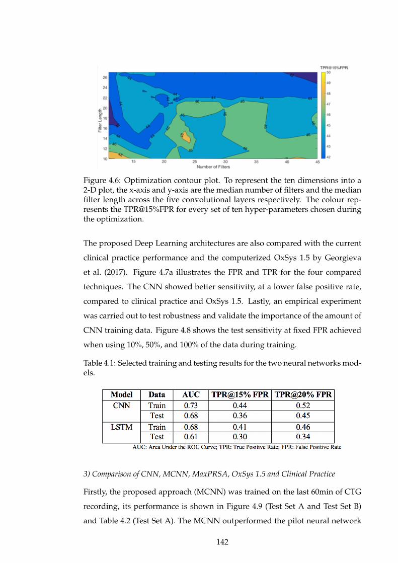
Figure 4.6: Optimization contour plot. To represent the ten dimensions into a2-D plot, the x-axis and y-axis are the median number of filters and the medianfilter length across the five convolutional layers respectively. The colour rep-resents the TPR@15%FPR for every set of ten hyper-parameters chosen duringthe optimization.

The proposed Deep Learning architectures are also compared with the current

clinical practice performance and the computerized OxSys 1.5 by Georgieva

et al. (2017). Figure 4.7a illustrates the FPR and TPR for the four compared

techniques. The CNN showed better sensitivity, at a lower false positive rate,

compared to clinical practice and OxSys 1.5. Lastly, an empirical experiment

was carried out to test robustness and validate the importance of the amount of

CNN training data. Figure 4.8 shows the test sensitivity at fixed FPR achieved

when using 10%, 50%, and 100% of the data during training.

Table 4.1: Selected training and testing results for the two neural networks mod-els.

3) Comparison of CNN, MCNN, MaxPRSA, OxSys 1.5 and Clinical Practice

Firstly, the proposed approach (MCNN) was trained on the last 60min of CTG

recording, its performance is shown in Figure 4.9 (Test Set A and Test Set B)

and Table 4.2 (Test Set A). The MCNN outperformed the pilot neural network

142

(a) (b)

Figure 4.7: Left: Comparison of the two Deep Learning models, OxSys 1.5 andClinical practice o the test set (x2 test for comparison of proportions); Right:ROC curves CNN vs LSTM models (Oxford test set: 5314 cases).

Figure 4.8: Robustness of CNN with respect to the size of training dataset over30 runs (FPR is fixed at 15%).

model, the single-channel CNN. The MCNN also outperformed clinical prac-

tice, maxPRSA (Georgieva et al., 2014) and Oxsys 1.5 (Georgieva et al., 2017), in-

creasing the TPR with the same or lower FPR. On Test Set B, CNN and MCNN

had poor sensitivity and OxSys 1.5 was strikingly better than all other meth-

ods, including clinical practice. This is not surprising, because these 40 severe

compromises without acidemia are a small and heterogeneous group better de-

tected with individualised rules for CTG interpretation in the clinical context

(as in OxSys 1.5).

143

(a) Test Set A, n=4429 (Normal/Moderateplus Severe Compr with pH<7.05)

(b) Test Set B, n=885 (Intermediate/SevereCompr. with pH>7.05)

Figure 4.9: Performance on last 60min of CTG: Clinical practice, MaxPRSA,Oxsys 1.5, CNN, MCNN, Stacked MCNN (median of 5 runs). The FPR wasfixed at 15% for the CNN and MCNN in order to be comparable to the FPR ofclinical practice.

Table 4.2: Comparison of the proposed models (median of 5 runs) on Test SetA (n=4429). Compromise: acidemia (arterial cord pH at birth <7.05); Normal:healthy new-born with arterial cord pH>7.15. FPR: false positive rate. Firstlabour stage: established labour before the onset of pushing. Second labourstage: pushing until birth.

144

Furthermore, I investigated the effect of labour stage on network performance

and whether it could improve if we analysed separately the end of the first and

second stages of labour. Firstly, the same experiment carried in the previous

section was replicated here but with training and testing only on data from the

first or second stage separately (two CNN and two MCNN models). The re-

sults in Table 4.2 show that the networks trained and tested on 2nd stage data

had higher TPR than the ones in 1st stage, which is to be expected because the

considered data are closer to the time of delivery when the outcome label is

assigned. Secondly, I trained a simple Stacked MCNN as shown in Figure 4.5,

using the MCNN model trained on 1st stage data to generate the probability for

compromise and then fed this as an additional feature into a 2nd stage MCNN

(trained and tested on 2nd stage with probability input from 1st stage when

available). The Stacked MCNN furtherly increased the AUC metric from 0.60

to 0.73 when compared to the MCNN trained on last hour in the 1st stage and

from 0.71 when compared to the same MCNN in the 2nd stage (Table 4.2). If

second stage data was not available (i.e. there was a Caesarean section in the

first stage), then the probability generated from the first stage analysis is used

for the final classification. In particular, in Test Set A, 6% of the data did not

have any 1st stage, while 29% did not have any 2nd stage. MCNN had AUC of

0.77 and Sensitivity of 53% for FPR@15% (Table 4.2) but, when the same MCNN

configuration was trained and tested only on the last one hour of 1st stage (not

the last hour of CTG recording), the AUC fell to 0.65 and the Sensitivity of 33%

at FPR@15%. Reduction in performance is to be expected when analysis moves

away from the time of birth and thus the outcome label (which is assigned at

birth): a compromise that was undetected in first stage may mean that the fe-

tus was still compensating well and the classification as normal was actually

correct at the time. On the other hand, when the MCNN model was trained

and tested only on the last 30min of 2nd stage (if 2nd stage was reached), the

MCNN achieved AUC of 0.70 and Sensitivity of 42%. So, the Stacked MCNN

improved on the individual MCNN performance in each labour stage but re-

mained slightly suboptimal when compared to the MCNN trained and tested

on the last hour (Table 4.2), AUC 0.74 vs 0.76 and Sensitivity for FPR@15% 47%

145

vs 53%. Only the median values were reported here because all networks had

very small performance variability over the five independent runs (0.1 and ±3.5

from the median for the AUC and TPR metrics respectively when trained on

the last 60min of CTG trace; ±0.2 and ±3.5 when trained on last 60min of first

stage). Finally, I concluded that the best performance was achieved with the

MCNN trained on the last 60min of CTG (regardless of stage).

4) Effect of the fetal heart rate signal quality on the classification threshold and MCNN

performance

Signal loss and noise are common in the fetal heart rate during labour moni-

toring. Basic pre-processing removed the noise and replaced it with missing

values (Georgieva et al., 2017). Thus I examined the influence of signal loss

(after de-noising) on the performance of my best model (MCNN trained on

the last 60min of CTG): I defined four groups of heart rate signal quality (Ta-

ble 4.3) based on the quality score vector (which consists of 10 values for 60min

monitoring corresponding to each 15min window moving with a 5min step). I

found that MCNN had consistently higher number of alerts (i.e. high-risk clas-

sifications) when there was more signal loss/noise (i.e. poorer signal quality).

Importantly, for every quality group there was a different probability cut off

point on the ROC curve (Figure 4.10) in order to obtain FPR at 15%. Without

the quality breakdown, it is only possible to select one (sub-optimal) cut point

for the different groups. It can be seen that the AUC is particularly low for

the group with poorest signal quality, clearly demonstrating the obvious - poor

signal quality leads to poor performance. Future work will focus on how to bet-

ter integrate the signal quality information into the MCNN, so that it is better

adjusted for.

5) Testing on external data

In addition to the Oxford Testing Set (>5000 CTGs), I tested my best model

(MCNN trained on the last 60min of CTG) and the corresponding Stacked MCNN

using two open access external datasets (SPaM’17, Table 4.4 and CTU-UHB, Ta-

ble 4.5). Currently, a publication is awaited for the SPaM’17 challenge that will

present all competing algorithms and performance in detail. However, the re-

146

Figure 4.10: ROC curves for the four quality groups (Testing Set A, n = 4429).

Table 4.3: Quality groups on Test Set A. For each quality group is reportedthe percentage of data belonging to that group and the TPR/FPR median (min- max) for the five runs. The median threshold for the MCNN classificationfor the five models was 0.50 with minimum and maximum of 0.47 and 0.53respectively (cases with higher than threshold MCNN value are classed as high-risk by the model).

sults were reported at the meeting in early Nov 2017 and I used them as a

general comparison. Both external sets have fetal compromise defined as cord

pH<7.05 and hence Test Set A is the testing set somewhat comparable to them.

The proposed models performed better on the SPaM dataset when compared to

Test Set A, but this is to be expected with such a selected set with high incidence

of cord pH<7.05 (20%, as opposed to 4% in Test Set A). It is interesting to note

that most of the methods performed substantially better on the data from Lyon,

when compared to the one from Brno and this is what can be also observed

with the proposed MCNNs (Table 4.4). On the Lyon data, four methods from

147

the SPaM challenge had TPR of 75% at FPR ranging between 20% - 24% and

one method achieved 95% TPR at 40%FPR. Therefore, both the MCNN and the

Stacked MCNN performed better - with 83% and 80% at 20%FPR (median val-

ues, Table 4.4). On the SPaM Brno data, the methods achieved TPR of 45% - 65%

with corresponding FPR of 12% - 29%FPR and this was only slightly improved

by my models.

Table 4.4: Testing on the SPaM’17 dataset. Reported is the median performancefor five models.

Table 4.5: Testing on the CTU-UHB dataset. Note this dataset also comes fromthe same Brno Hospital but there is no overlap with the SPaM17 data.

The MCNN and Stacked MCNN methods performed a little bit better on the

CTU-UHB dataset than on the SPaM subset coming from the same hospital

(Brno). I found two published methods reporting results on the CTU-UHB

database (even though the data was not strictly used as an unseen testing set)

and compared to them: Spilka et al (Spilka et al., 2016) reported 40% TPR at 14%

FPR and Georgoulas et al (Georgoulas et al., 2017) reported 72%TPR at 35%FPR.

The proposed Deep Learning approaches performed substantially better: the

MCNN had 58% (53% - 60%) at 14%FPR and 80% (75% - 85%) at 35%FPR; and

the Stacked MCNN had 55% (53% - 60%) at 14%FPR and 83% (75% - 88%) at

35%FPR.

148

4.1.6 Discussion

The CTG analysis during labour still relies on visual examination of long and

complex heart rate patterns: a massive clinical challenge which has seen vir-

tually no improvements in the past decades (Timmins and Clark, 2015). There

have been developments of computer-based methods who are designed to mimic

clinical interpretation and assist the visual CTG assessment by highlighting/alerting

features of interest, but these have shown no benefit in clinical practice (Brock-

lehurst et al., 2017; Nunes et al., 2017). Data-driven CTG analysis is still a nar-

row and challenging field with only a few teams working with CTG datasets of

about 3000 CTGs, in contrast, here I present my work on Deep Learning meth-

ods employing more than 35000 CTG samples.

The motivation behind the initial pilot study (point 2) on CNN and LSTM was

to move away from classic feature extraction approaches and examine whether

Deep Learning has the potential to detect information in the EFM that is cur-

rently “hidden”. Both architectures showed good generalizability - retaining

similar performance on training and testing (Table 4.1). On the Oxford data,

CNN performed better than the LSTM (Table 4.1, Figure 4.7a, Figure 4.7b). Also,

CNN outperformed the results of clinical practice (Figure 4.7a) and showed ro-

bust performance (Figure 4.8). As can be seen from Figure 4.8, the sensitivity

of CNN increased and its variance decreased with larger size of the training

set. Direct comparison with OxSys 1.5 suggested that CNN achieved better

results, but this must be interpreted with caution because OxSys 1.5 is based

on the entire dataset and analyses the entire EFM trace, incorporating clinical

risk factors. The CNN’s TPR of 44% @15%FPR (Figure 4.7a) is significantly

higher than the TPR in clinical practice (31%) but needs to exceed 60% if we

want tangible clinical benefits. Furthermore, I developed Multimodal Convo-

lutional Neural Networks (MCNN) and Stacked MCNN models for the pre-

diction of fetal compromise, using CTG traces from >35000 labours (85% for

training and 15% for testing). The Stacked MCNN, is a more clinically rele-

vant model allowing the analysis of the CTGs from first and second labour

stages separately and feeding the estimated probability for compromise from

149

first stage into the analysis of the second labour stage. The MCNN is a more

flexible network architecture, compared to the single channel CNN, allowing

inputs with different dimensions. Thus, in addition to the fetal heart rate and

contraction signals, a third input is used, indicating the signal quality vector

containing the rate of signal loss in the fetal heart rate trace. The MCNNs’ con-

volutional layer hyper-parameters (i.e., number of filters and filter length) were

independently optimized for each layer, granting more flexibility during the

network optimization when compared to the CNN model (Section 4.1.5, point

2). The optimization of the convolutional layers (Figure 4.6) showed the MCNN

to work better when using many short filters on the contrary of what was found

in Section 4.1.5 (point 1) where the CNN was working better with few large fil-

ters. This is probably due to the fact that each layer here was independently

optimized, allowing for different filter length and number of filters. This find-

ing could also be explained by the different architecture proposed here, where

each input is treated separately before the fully connected layer. On the Ox-

ford Testing Set of >5000 births, I compared the results of the proposed models

with: clinical practice as well as the current Oxford prototype system OxSys 1.5

by Georgieva et al. (2017), the maximal Phase Rectified Signal Averaging (max-

PRSA, (Georgieva et al., 2014)) and single channel CNN. Even though I trained

the models with all available training data, I reported the testing results on the

testing set split into two exclusive groups (Set A and Set B) according to the

definition of compromise demonstrating the usefulness of such separation, as

explained below. Firstly, for the prediction of acidemia (cord pH<7.05) with or

without severe compromise (Test Set A, n = 4429 births), all neural networks

performed substantially better than clinical practice, MaxPRSA or OxSys 1.5,

with TPR at least 20% higher than that of clinical practice for the same or lower

FPR, i.e. TPR of 53% vs 31% for MCNN and clinical practice respectively (Fig-

ure 4.9a). The best performing model was the newly proposed MCNN, trained

on the last 60min of CTG regardless of the labour stage (Figure 4.9a and Ta-

ble 4.2). Thus, the MCNN outperformed also the Stacked MCNN (53% vs 47%

TPR at 15%FPR, Figure 4.9a). There are several explanations for this. The main

challenge with analysing the second stage separately is the different duration

150

for each labour (most labours have between 10min to 150min of 2nd stage). The

proposed Stacked MCNN analysed strictly only the last 30min, padding with

zeros at the beginning if there was less than 30min recording in the 2nd stage.

This introduced a gap of CTG data not analysed by the Stacked MCNN model,

potentially losing information. Future work will examine more flexible models

of the stacked approach, allowing for iterative analysis of the entire CTG avail-

able. Even though it could not outperform the MCNN trained on last 60min

labour, the Stacked MCNN model performed well and provided a first attempt

to analyse the CTG by estimating the probability of compromise at a point in

time by using probability estimates from CTG data at an earlier time. I believe

that as a concept and with future work, such stacked models could provide a

clinically relevant model suitable for use at the bedside, building on the time se-

ries nature of the CTG (often >15hours long). Furthermore, I showed that noisy

and inaccurate signal (i.e., high number of missing measurements) negatively

impacts the performance of the models (Figure 4.10, Table 4.3). My models

were more likely to class a trace as abnormal if the heart rate had poor quality,

indicating that future models could benefit from adjustments to remove this

bias. Secondly, for the detection of severe compromise without acidemia (Test

Set B, n = 845 births, Figure 4.9b), all neural networks had low TPR. OxSys 1.5

was the best at 45% followed by clinical practice at 33% and the Deep Learning

models around 20% TPR, for the same FPR. The Severe compromises without

acidemia are a heterogeneous and challenging group to detect. They seem bet-

ter suited to be detected by tailored diagnostic rules such as the ones in OxSys

1.5, which incorporates clinical risk factors and analyses the entire CTG trace

from the beginning (for example, some pre-existing fetal injuries are detected

by OxSys 1.5 early on in the CTG and are irrelevant to the proposed here mod-

els). I conclude that future work should focus on improving performance on

both test sets separately, with highest gain from CNN-based approaches po-

tentially for detecting the more homogeneous problem of acidemia. The cur-

rent FPR in clinical practice of >15% is unacceptably high and future work

will consider improving my network models working towards a new gener-

ation OxSys system, incorporating the best from both - Deep Learning black box

151

models and from heuristic domain-based knowledge. Finally, I used two open

access datasets for testing my methods, allowing a comparison with work from

other researchers and setting a standard for future comparisons: SPaM dataset

(Brno and Lyon subsets, a total of 200 high quality CTGs with 20% incidence

of compromise, cord pH<7.05); and the CTU-UHB dataset (552 CTGs with 7%

incidence of cord pH<7.05). I concluded that the MCNN models convincingly

outperformed the methods which competed in the SPaM challenge and any

limited results reported on the CTU-UHB dataset. This was so even though

both for the SPaM and CTU-UHB, many researchers did not use the data as

set-aside testing sets but also used it for training/tuning one way or another.

4.2 Deep Learning for stock market volatility fore-casting

Quantifying the potential loss of assets is a big part of risk management, trad-

ing in financial markets and asset allocation. To be able to measure these losses

and make investment decisions, investors need to estimate risks (Blume, 1971).

Since volatility has some well-known statistical regularities that make it inher-

ently forecastable, it is among one of the most accepted and used measures of

risk in the financial market. These regularities include the volatility clustering

effect, leading to positive and persistent autocorrelations of volatility measures,

the leverage effect, which is related to the negative correlation between past re-

turns and current volatility values, the dynamic cross-correlation between the

volatilities of different assets that give rise to the well-known phenomenon of

volatility spillovers. In addition, it is worth reminding that volatility is a key

ingredient for computing more refined risk measures such as the Value at Risk

or the Expected Shortfall.

As the prediction of volatility is a major factor in risk analysis, many efforts

have been made to implement parametric as well as non-parametric predictive

methods for forecasting future volatility. Depending on the reference informa-

tion set, the proposed approaches can be classified into two broad categories. Of

these, the first includes approaches fitted to time series of daily log-returns. In

152

the parametric world, this class of methods includes the Generalized Autore-

gressive Conditionally Heteroskedastic (GARCH) models of Bollerslev (1986)

and their numerous univariate and multivariate extensions (Bauwens et al.,

2006) while, in the non-parametric world, I recall a consistent number of papers

applying non-parametric approximators (such as smoothing splines (Langrock

et al., 2015; Zhang and Teo, 2015) or neural networks to time series (Wang et al.,

2015; Kourentzes et al., 2014)) of squared returns taken here as an unbiased, but

noisy volatility proxy.

The second and more recent class of approaches for volatility forecasting re-

places this noisy volatility proxy with more efficient realized volatility mea-

sures (Andersen and Terasvirta, 2009) built from time series of high-frequency

asset prices. Notable examples of parametric models falling into this second

class of approaches are the class of Multiplicative Error Models (MEM) by En-

gle and Russell (1998) and the Realized GARCH (R-GARCH) models (Hansen

et al., 2012). The main structural difference between MEM and R-GARCH mod-

els is that, differently from the R-GARCH which uses bivariate information on

log-returns and realised volatility, the MEM are directly fitted to a univariate re-

alised volatility series, and log-returns are eventually used only as external re-

gressors for capturing leverage effects. Similarly, in a non-parametric environ-

ment, neural networks (McAleer and Medeiros, 2011) or other non-parametric

filters (Chen et al., 2018) can be applied to time series of realised volatility

measures to forecast future volatility. See also (Han and Zhang, 2012) non-

parametric volatility modelling for non-stationary time series.

All above-discussed approaches are univariate. Nevertheless, the presence of

phenomena such as common features and volatility spillovers make the analy-

sis of multivariate volatility panels potentially very profitable. In a parametric

setting, however, the number of required model parameters is rapidly explod-

ing as the cross-sectional dimension of the panel increases, making the estima-

tion infeasible even for moderately large dimensions, unless some heavy, and

untested parametric restrictions are imposed. Typically, it is often assumed that

all the volatilities in the panel share the same dynamic dependence structure

153

and volatility spillovers are not present (Pakel et al., 2011). Those assumptions

are clearly unrealistic and they greatly reduce the ability of parametric models,

albeit multivariate, to describe the complexity of the dynamic structure which

is observed in financial time series.

Feed-forward neural networks are a favourite class of multivariate, non-parametric

models used to study dependencies and trends in the data, e.g. using mul-

tiple inputs from the past to predict the future time step (Chakraborty et al.,

1992). However, when using traditional neural network models, much effort

is devoted to make sure that what is presented for training in the input layer

is already in a format that allows the network to recognise the significant pat-

terns. This process usually requires some ad-hoc procedures and soon becomes

one of the most time-consuming part of neural network modelling. In a Deep

Learning framework instead, by adding more and more layers between input

and output (hence “deep”), the model allows richer intermediate representa-

tions to be built and most of that feature engineering process can be achieved

by the algorithm itself, in an almost automatic fashion. This latter point both

improves prediction accuracy and strongly widens the domains of applications.

As a drawback, Deep Learning models require a large amount of data to out-

perform other approaches and are computationally expensive to train. How-

ever, the availability of parallel computing, both on CPUs and GPUs, sharply

reduces the computational burden making even complex Deep Learning train-

ing processes feasible. Moreover, in financial applications a large amount of

data can be quickly gathered, making Deep Learning applications appropriate

and viable.

The main focus of this work is on proving the effectiveness of using Deep

Learning techniques for multivariate time series forecasting. In particular, a

stacked LSTM is applied for forecasting the volatility of financial time series.

The LSTMs have several advantages with respect to the modelling approaches

used so far in the literature. Firstly, they can be seen as non-parametric statis-

tical models, and consequently, they do not suffer from the misspecification

problems which typically affects parametric modelling strategies. Secondly,

154

they can overcome the curse of dimensionality problem which affects both stan-

dard non-parametric estimation techniques and several multivariate paramet-

ric models (Poggio et al., 2017), making the use of LSTMs feasible even for high

dimensional temporal datasets. Moreover, they do not require any undesirable

reduction of the parameter space through untestable, unrealistic restrictions,

which might significantly reduce the ability of the model to reveal some well-

known stylized facts about multivariate financial time series (such as spillovers

and complex dynamics). Finally, they can profit from modelling complex non-

linear and long-term dependencies, leading to improved accurate predictions

(Gers et al., 2002a).

4.2.1 Data

Two datasets are used for the empirical experimentation. The first dataset used

by Hansen et al. (2012), includes 28 assets from the Dow Jones Industrial Av-

erage (DJI 500) index plus one exchange-traded index fund SPY, that tracks the

S&P 500 index. The sample spans the period from 1st January 2002 to 31st Au-

gust 2008. The second dataset is related to 92 stocks belonging to the NASDAQ

100 index within the period 1st December 2012 to 29th November 2017. Further

detail on the two datasets can be found in Table 4.6 and Table 4.7 respectively1.

Each asset is represented by two different time series, the realized measure,

namely volatility, and the related open-close return. The realized measure vt is

given by a realized kernel estimator computed using the Parzen kernel func-

tion. This estimator is similar to the realized variance, and more importantly, it

is robust to market micro-structure noise and is more accurate than the quadratic

variation estimator. The implementation of the realized kernel follows the method

proposed by Barndorff-Nielsen et al. (2011) that guarantees a positive estimate.

1The data is publicly available on the following Zenodo repositoryhttps://zenodo.org/record/2540818

155

Table 4.6: Dow Jones Industrial Average assets used as case study. Capitaliza-tion is given with respect to 4th August 2017 values.

Symbol Name Sector Capitalization (USD)

AA Alcoa Corp Materials 6.89BAIG American International Group Financials 58.79BAXP American Express Financials 75.99BBA Boeing Industrials 140.50BBAC Bank of America Financials 245.97BC Citigroup Financials 187.94BCAT Caterpillar Industrials 67.58BCVX Chevron Energy 208.66BDD EI du Pont de Nemours Materials 71.17BDIS Disney Consumer Discretionary 168.52BGE General Electric Industrials 223.20BGM General Motors Consumer Discretionary 51.39BHD Home Depot Consumer Discretionary 182.62BIBM IBM Information Technology 135.28BINTC Intel Information Technology 170.57BJNJ Johnson & Johnson Health Care 357.45BJPM JPMorgan Chase Financials 329.58BKO Coca-Cola Consumer Staples 194.07BMCD McDonald’s Consumer Discretionary 125.37BMMM 3M Industrials 123.92BMRK Merck Health Care 172.59BMSFT Microsoft Information Technology 559.80BPG Procter & Gamble Consumer Staples 231.51BT AT&T Telecommunication Services 235.96BUTX United Technologies Industrials 97.04BVZ Verizon Telecommunication Services 199.52BWMT Wal-Mart Consumer Staples 242.61BXOM Exxon Mobil Energy 339.86B

SPY SPDR S&P500 ETF Trust - (Net Assets) 242,54B

4.2.2 Experimental setup

The proposed model is a 2-layer stacked LSTM made of 2n and n units respec-

tively, with n being the number of assets, according to the input and output

size. This means 58/29 for DJI 500 and 184/92 for NASDAQ 100. The output of

the first LSTM is given as input to a dense activation layer designed to provide

the model’s output (Figure 4.11 shows a schematic description of the model).

The hidden activation function is an hyperbolic tangent, while the recurrent ac-

tivation is a hard sigmoid (default activation functions for LSTM, as advised

by Hochreiter and Schmidhuber (1997)). To avoid negative forecasts (the real-

ized volatility is always continuous positive), a softplus function is used in the

output layer.

Two topologies of LSTM are tested and evaluated: univariate and multivariate.

LSTM-1: A univariate architecture (one model independently trained for each

asset) taking as input only one asset at the time (open-close return and volatility

156

Table 4.7: NASDAQ 100 assets used as case study.

Sector Symbol

Capital Goods ILMN, KLAC, PCAR, PCLN, TSLAConsumer Non-Durables CTAS, HAS, MDLZ, MNSTConsumer Services AMZN, CHTR, CMCSA, COST, DISCA, DISCK, DISH,

DLTR, EXPE, FAST, FOXA, FOX, LBTYA, LBTYK,LVNTA, NFLX, ORLY, PAYX, QVCA, ROST,SBUX, SIRI, TSCO, ULTA, VIAB, WYNN

Health Care ALGN, ALXN, AMGN, BIIB, CELG, ESRX, GILD,HOLX, HSIC, IDXX, INCY, ISRG, MYL, SHPG, XRAY

Miscellaneous AKAM, CTRP, EBAY, MELI, NTESPublic Utilities VODTechnology AAPL, ADBE, ADI, ADP, ADSK, AMAT, ATVI,

AVGO, BIDU, CA, CERN, CHKP, CSCO, CTSH,CTXS, EA, FB, FISV, GOOGL, INTC, INTU,LRCX, MCHP, MSFT, MU, MXIM, NVDA, QCOM,STX, SWKS, SYMC, TXN, VRSK, WDC, XLNX

Transportation JBHT

for a chosen past window (rt-k, .., rt-1, vt-k, .., vt-1) and producing as output

the one-step-ahead volatility (vt).

LSTM-n: A multivariate architecture, where a single model is trained using all

the assets. This version takes as input the open-close return and volatility for

a given past window (rit-k, .., rit-1, vit-k, .., vit-1), i = 1, . . . ,n and outputting the

n one-step-ahead volatilities (vit, i = 1, . . . ,n), where n = 29 for DJI 500 and

n = 92 for NASDAQ 100.

Figure 4.11: The proposed model for DJI 500 is a stack of two LSTM with 58 and29 neurons each and a dense activation layer on the top. The size of the denselayer is one in the univariate approach (LSTM-1) and 29 in the multivariate one(LSTM-29).

The model is pre-trained by using the first 300 days of the dataset with a look-

back window of 20 days. Subsequently, a rolling forecast is applied from day

301 onward. In particular, every time the one-step-ahead volatility is predicted,

its observed features (realized return and volatility) are used to refine the net-

work state, before moving the time window one step. This procedure allows

having an up-to-date network, every time new information is available.

The hyper-parameters of the network have been optimised using a grid search,

157

Table 4.8: Hyper-parameters for the LSTM. The optimal value of each hyper-parameter has been selected through a grid search on the defined range.

Hyper-parameter Range of optimization Optimal value

Dropout [0, 0.6] every 0.1 0.2Number of training epochs on pre-training data [100, 400] every 50 300Number of training epochs on rolling window [10, 30] every 5 20Look-back [5, 100] every 5 20Loss function MSE and QLIKE QLIKE

and their search boundaries and optimal values are reported in Table 4.8. The

optimal number of training epochs on the initial data was found to be in line

with the optimal number of days used for pre-training (i.e., 300 days), while the

number of epochs for the rolling period had its best value consistent with the

size of the look-back (i.e., 20 days, equivalent to four weeks of trading data). I

observed that a smaller number of epochs would produce an under-fitted net-

work (smooth forecast trending with the average of the last few data points),

while a longer training would produce an over-fitting network (giving a lot of

weight to the most recently shown data point). Furthermore, a larger look-back

would impact the convergency (probably due to the vanishing gradient prob-

lem). In addition, dropout, a standard regularization technique used for Deep

Learning models, was used to avoid over-fitting, and its best value was found

to be around 0.20, as also suggested by Wan et al. (2013). Lastly, I used two loss

functions to train the model: MSE and QLIKE.

Both online and offline evaluations have been considered to assess the model

performance. In the online evaluation case, two alternative fitness functions

have been used to train the LSTM models: the widely used MSE for regression

and forecasting tasks (described in Section 2.5.2); and the QLIKE loss function,

particularly suitable for volatility forecasting (Patton, 2011). For the offline eval-

uation case, a test data set (not used for training) for out-of-sample evaluation

using MSE, QLIKE and the Pearson correlation index is considered.

Given a vector Y of N forecasts and the vector Y of observed values, the QLIKE

is defined a follows:

QLIKE =1N

NX

i=1

(log(Yi) +Yi

Yi). (39)

158

Both MSE and QLIKE measures are proposed in the evaluation framework

since they are considered to be robust for assessing volatility forecast perfor-

mance (Patton, 2011). A robust measure must ensure that using a proxy for the

volatility (the realized kernel in this case) gives the same ranking as using the

true (unobservable) volatility of an asset.

Moreover, the Pearson correlation coefficient is computed between the forecast

volatility of each estimated model and the realized one, to assess the ability of

the models to follow the assets trends.

Lastly, the Diebold-Mariano (DM) test is used to assess models’ conditional pre-

dictive ability. The one tail DM is used with squared error, predictive horizon

equal to 1 (for one step ahead forecast) and a significance threshold at 0.05,

to test the following NULL hypothesis ‘Model Mi has better predictive ability

than model Mj with a size level equal to ↵ = 0.05’.

Before training the model, the data are normalised and standardised with 0-

mean and 1-variance. Since the features are in IR+, for each sample (rt, vt), its

negative (-rt, -vt) is added to the data (to have a perfectly bell shaped distri-

bution). The resulting distribution is already mean-centred, hence the values

are divided by their standard deviation and finally, the added negative values

are dropped to restore the original set of observations.

4.2.3 Compared methods

a) Realized Garch (R-GARCH)

The Realized GARCH introduced by (Hansen et al., 2012) has extended the

class of GARCH models by replacing, in the volatility dynamics, the squared

returns with a much more efficient proxy such as a realized volatility measure.

The structure of the R-GARCH(p, q) in its linear formulation is given by:

rt = µ+p

ht zt, (40)

ht = !+�ht-1 + � vt-1, (41)

vt = ⇠+'ht + ⌧(zt) + ut, (42)

159

where zt⇠i.i.d.(0, 1) and ut⇠i.i.d.(0,�2u) with zt and ut being mutually inde-

pendent. The first two equations are the return equation and the volatility equa-

tion that define a class of GARCH-X models, including those estimated in (En-

gle, 2002; Barndorff-Nielsen and Shephard, 2005; Visser, 2011). The GARCH-X

acronym refers to the fact that vt is treated as an exogenous variable. It is worth

noting that most variants of ARCH and GARCH models are nested in the R-

GARCH framework. The measurement equation is justified by the fact that

any consistent estimator of the Integrated variance can be written as the sum of

the conditional variance plus a random innovation, where the latter is captured

by ⌧(zt) + ut. The function ⌧(zt) can accommodate leverage effects, because

it captures the dependence between returns and future volatility. A common

choice (Hansen et al., 2012), that has been found to be empirically satisfactory,

is to use the specification:

⌧(zt) = ⌧1 zt + ⌧2(z2t - 1). (43)

Substituting the measurement equation into the volatility equation, it can be

easily shown that the model implies an AR(1) representation of ht:

ht = (!+ ⇠�) + (�+'�)ht-1 + �wt-1, (44)

where wt = ⌧(zt) + ut. Furthermore it is assumed that the expectation of

E(wt) = 0. The coefficient (�+'�) reflects the persistence of volatility, whereas

� summarizes the impact of the past realized measure on future volatility.

The general conditions required to ensure that the volatility process ht is sta-

tionary and the unconditional variance of rt is finite and positive are given by:

!+ ⇠� > 0, (45)

0 < �+'� < 1. (46)

160

If the conditions in Eq. 45 are fulfilled, the unconditional variance of rt, tak-

ing expectations of both sides in Eq. 44, can be easily shown to be equal to

(!+ ⇠�)/[1- (�+'�)]. Finally, as for standard GARCH models, the positivity

of ht (8t) is achieved under the general condition that !, � and � are all posi-

tive.

b) GJR-MEM

Multiplicative Error Models (MEM) were first proposed by Engle (2002) as a

generalization to non-negative variables of the Autoregressive Conditional Du-

ration models of Engle and Russell (1998). Namely, let vt be a discrete time

process on [0,1) (e.g. a realized measure). A general formulation of the MEM

is

vt = µt✏t, (47)

µt = µ( µ, It-1), (48)

where (✏t|It-1)iid⇠ D+(1,�2). It can be easily seen that

E[vt|It-1] = µt, (49)

var[vt|It-1] = �2µ2t , (50)

where the conditional expectation of the realized measure (µt) provides an es-

timate of the latent conditional variance ht.

The GJR-MEM model is obtained by borrowing from the GARCH literature

(Glosten et al., 1993; Engle, 2002) the following dynamic equation for µt:

µt = !+↵vt-1 +�µt-1 + �vt-1I(rt-1 < 0), (51)

which allows to reproduce volatility clustering as well as leverage effects.

Coming to the specification of the distribution of ✏t, any unit mean distribution

with positive support could be used. Possible choices include Gamma, Log-

161

Normal, Weibull, Inverted-Gamma and mixtures of them. In this experiments I

consider the Gamma distribution which is a flexible choice able to fit a variety

of empirical settings. If (✏t|It-1) ⇠ �(✓,�), its density would be given by

f(✏t|It-1) =1

�(✓)�✓✏✓-1t exp

✓-✏t�

◆(52)

However, since E(✏t|It-1) = ✓�, to ensure unit mean, it is needed to impose the

constraint � = 1/✓ giving rise to the following density

f(✏t|It-1) =1

�(✓)✓✓✏✓-1

t exp (-✓✏t). (53)

Model parameters can be then estimated maximizing the likelihood function

implied by the unit mean Gamma assumption. It is worth noting that these

estimates have a quasi maximum likelihood interpretation since it can be shown

that, given that µt is correctly specified, they are still consistent and asymptotic

normal even if the distribution of ✏t is misspecified.

c) Elman Recurrent Neural Networks (RNN)

The Elman Network (also known as Simple Recurrent Network) is one of the

most basic RNN architectures known in literature. Its topology consists of three

layers (i.e., input, hidden, and output) with the addition of a set of context

units (i.e., the network state). The state saves a copy of the previous values

of the hidden units allowing interactions with the current inputs. Thus this

architecture can be considered a very simplified version of the LSTM, where

only information of the most recent past is stored.

ht =�h(Whxt +Uhht-1 + bh), (54)

yt =�y(Wyht + by) (55)

162

4.2.4 Results and discussion

In this section, the proposed approach to forecast stock market volatility, based

on deep neural networks, is implemented in two variants: univariate (LSTM-

1) and multivariate (LSTM-29 and LSTM-92). The method is compared with

two state of the art methodologies, namely R-GARCH (Hansen et al., 2012) and

GJR-MEM (Glosten et al., 1993). Here I discuss empirical results from an out-

of-sample forecasting comparison, using returns and realized measures for the

28 Dow Jones Industrial Average stocks and one exchange-traded index fund,

SPY, which tracks the S&P 500 index over a period of 1250 days and for the 92

stocks belonging to the NASDAQ 100 index over a period of 956 days.

a) Dow Jones Industrial Average 500

Table 4.9: Evaluation Metrics for the DJI 500 dataset: The MSE, QLIKE andPearson measures are reported for each asset and for each compared model.

Asset LSTM-1 LSTM-29 R-GARCH GJR-MEM

MSE QLIKE Pearson MSE QLIKE Pearson MSE QLIKE Pearson MSE QLIKE Pearson

AA 4.77 1.98716 0.59 3.65 1.97534 0.69 4.83 2.01253 0.60 4.05 1.97021 0.65AIG 6.71 1.40473 0.61 4.84 1.35021 0.72 6.40 1.43038 0.61 5.40 1.35342 0.70AXP 3.19 1.12222 0.77 1.70 1.10570 0.87 2.11 1.11389 0.84 2.00 1.10602 0.85BA 0.88 1.40893 0.56 0.81 1.40138 0.62 0.85 1.41024 0.59 0.80 1.40229 0.62BAC 3.93 0.91670 0.73 2.86 0.88778 0.81 5.19 0.96517 0.71 3.35 0.89910 0.77C 5.86 1.21826 0.74 2.48 1.18877 0.89 3.62 1.22085 0.83 2.92 1.19124 0.86CAT 1.12 1.56860 0.65 1.03 1.55595 0.69 1.18 1.56885 0.62 1.10 1.55946 0.66CVX 1.36 1.32972 0.69 1.05 1.32618 0.76 1.20 1.32096 0.72 1.07 1.31349 0.75DD 1.56 1.31255 0.64 1.10 1.29515 0.76 1.33 1.32252 0.72 1.11 1.29064 0.75DIS 1.01 1.35000 0.52 0.86 1.33076 0.63 0.88 1.33510 0.61 0.83 1.32302 0.63GE 0.57 0.92743 0.66 0.50 0.92145 0.72 0.54 0.93285 0.69 0.50 0.91087 0.71GM 11.44 2.14155 0.62 9.83 2.10353 0.68 11.45 2.10482 0.62 10.79 2.09708 0.64HD 2.58 1.56234 0.68 1.83 1.55630 0.78 1.99 1.55294 0.76 1.81 1.54174 0.77IBM 0.65 1.00420 0.64 0.51 0.99950 0.73 0.65 1.01651 0.64 0.54 0.98996 0.70INTC 1.42 1.77012 0.62 1.52 1.77107 0.62 1.51 1.77072 0.59 1.40 1.76207 0.62JNJ 0.33 0.60274 0.52 0.32 0.60311 0.54 0.35 0.65656 0.48 0.34 0.60319 0.51JPM 4.92 1.31900 0.76 3.86 1.30975 0.80 4.27 1.32231 0.78 3.24 1.29987 0.84KO 0.28 0.76443 0.59 0.27 0.76449 0.61 0.34 0.83988 0.56 0.27 0.75574 0.60MCD 1.32 1.35511 0.49 1.40 1.37356 0.48 1.32 1.36301 0.49 1.41 1.35786 0.47MMM 0.64 1.05299 0.56 0.55 1.05117 0.65 0.68 1.09912 0.55 0.54 1.04440 0.64MRK 9.45 1.55236 0.25 8.63 1.54827 0.38 9.75 1.57830 0.26 10.30 1.53410 0.28MSFT 0.77 1.20058 0.60 0.63 1.20299 0.69 0.63 1.20704 0.68 0.57 1.18384 0.70PG 0.25 0.76355 0.56 0.25 0.76961 0.58 0.31 0.80720 0.52 0.25 0.75837 0.57SPY 0.17 0.16199 0.72 0.17 0.15189 0.75 0.16 0.13691 0.75 0.14 0.12674 0.78T 1.97 1.44030 0.63 1.64 1.43042 0.70 2.12 1.46438 0.63 1.72 1.42659 0.69UTX 0.85 1.17023 0.50 0.69 1.16343 0.62 0.97 1.18749 0.47 0.74 1.15846 0.59VZ 1.40 1.26611 0.54 1.05 1.26430 0.70 1.15 1.29074 0.67 1.02 1.25300 0.70WMT 0.71 1.12620 0.64 0.67 1.12532 0.68 0.88 1.16037 0.60 0.70 1.11630 0.65XOM 0.95 1.24535 0.71 0.89 1.24840 0.73 0.92 1.23848 0.71 0.87 1.23240 0.73

A detailed comparison of the methods performance is given in Table 4.9 with

respect to each asset. The LSTM-29 approach reaches the lowest MSE error

for 18 out of the 29 assets when compared with LSTM-1, R-GARCH and GJR-

163

Figure 4.12: LSTM-29 one step ahead predictions for all assets of the DJI 500dataset (excluded the index fund SPY). The observed time series are given ingray and the predicted volatility values in black.

MEM methods. In particular, the LSTM-29 has a lower error compared to the

proposed univariate model for 25 out of 29 assets, equal in 2 and worse in 2

cases. Compared to R-GARCH, the LSTM-29 is better again in 25 out of 29

cases, equal for 1, and worse for 3 assets. Lastly, the multivariate LSTM is better,

equal and worse than GJR-MEM in 16, 3 and 10 cases respectively. The one step

ahead prediction given by the LSTM-29 is presented in Figure 4.12.

Having a closer look at the MSE values from Table 4.9, the LSTM-29 is not better

than the other benchmarks on assets with very low errors and hence volatility,

in the considered period (e.g., JNJ, KO, PG, and SPY).

164

0

5

10

15

0 1 2 3MSEdeviation

Variability

(a) LSTM-1

0

5

10

15

0.0 0.5 1.0 1.5 2.0MSEdeviation

Variability

(b) R-GARCH

0

5

10

15

0 1MSEdeviation

Variability

(c) GJR-MEM

Figure 4.13: Relationship between difference in MSE (for LSTM-29 vs: LSTM-1(Figure 4.13a); R-GARCH (Figure 4.13b); and GJR-MEM (Figure 4.13c)) (y-axis)and variance of volatility (x-axis). Each dot represents an asset. LSTM-29 getsbetter in periods of high volatility.

Figure 4.13 is a scatter plot illustration comparing for each asset, the perfor-

mance of the LSTM-29 and the other models measured in terms of MSE differ-

ence (i.e., positive values representing smaller errors and better LSTM-29 per-

formance) versus asset volatility in terms of its variance (i.e., higher values of

variance representing stronger fluctuation in daily volatilities) over the out of

sample period (1250 days).

As can be seen from Figure 4.13, the LSTM-29 is generally comparable with

the other models at lower volatility, while outperforming the LSTM-1 and the

two state-of-the-art R-GARCH and GJR-MEM approaches in higher volatility

regimes. This result is confirmed by the Pearson’s correlation index with values

0.825 against LSTM-1, 0.800 against R-GARCH, and 0.608 against GJR-MEM

over the 29 assets.

To verify whether the proposed approach has statistically superior predictive

ability, a Diebold-Mariano test is performed using a predictive horizon equal

to 1 (one-step-ahead forecast). As it can be observed from the results reported

in Table 4.10, the LSTM-29 has a better predictive ability for 10 out of 29 assets

compared to the LSTM-1, 16 over 29 against the R-GARCH, and 6 out of 29

assets for the GJR-MEM, when considering a p-value strictly lower than 0.05. It

is also worth noticing that in the remaining cases LSTM-29 is never worse than

the compared models.

165

Table 4.10: Debold-Mariano statistic for the DJI 500 dataset (with a p-valuegiven in brackets) for the LSTM-29 against LSTM-1, R-GARCH and GJR-MEM.The p-values are marked with a * for 10% confidence level, with ** for 5% andwith *** for 1%.

Asset LSTM-29 vs.

LSTM-1 R-GARCH GJR-MEM

AA -2.42 (0.008***) -3.21 (0.001***) -2.53 (0.006***)AIG -2.86 (0.002***) -2.35 (0.009***) -1.21 (0.114)AXP -2.68 (0.004***) -2.76 (0.003***) -2.06 (0.020**)BA -1.33 (0.092*) -1.92 (0.028**) 0.25 (0.597)BAC -2.27 (0.012**) -3.11 (0.001***) -1.65 (0.049**)C -3.12 (0.001***) -3.33 (0.000***) -2.17 (0.015**)CAT -1.01 (0.157) -2.45 (0.007***) -1.28 (0.100*)CVX -1.60 (0.055*) -1.54 (0.061*) -0.20 (0.420)DD -1.77 (0.039**) -2.51 (0.006***) -0.18 (0.429)DIS -1.55 (0.060*) -0.62 (0.267) 0.64 (0.739)GE -0.85 (0.198) -0.85 (0.197) -0.10 (0.460)GM -2.12 (0.017**) -2.91 (0.002***) -2.05 (0.020**)HD -1.67 (0.048**) -1.03 (0.153) 0.14 (0.556)IBM -1.81 (0.035**) -2.31 (0.011**) -0.89 (0.187)INTC 0.64 (0.740) 0.05 (0.520) 1.27 (0.898)JNJ -0.10 (0.458) -1.27 (0.100*) -1.69 (0.046**)JPM -1.29 (0.099*) -1.37 (0.085*) 1.28 (0.900)KO -0.28 (0.389) -2.9 (0.002***) -0.44 (0.331)MCD 1.27 (0.898) 1.52 (0.935) -0.14 (0.443)MMM -1.46 (0.072*) -2.36 (0.009***) 0.33 (0.628)MRK -0.97 (0.165) -1.47 (0.071**) -1.58 (0.057*)MSFT -0.93 (0.176) 0.02 (0.509) 1.38 (0.916)PG -0.36 (0.360) -3.00 (0.001***) 0.00 (0.501)SPY -0.09 (0.463) 0.33 (0.629) 1.92 (0.972)T -1.76 (0.040**) -2.72 (0.003***) -1.20 (0.116)UTX -0.87 (0.192) -1.72 (0.043**) -0.94 (0.173)VZ -1.45 (0.074*) -1.02 (0.153) 0.58 (0.718)WMT -0.74 (0.230) -2.26 (0.012**) -0.61 (0.272)XOM -0.54 (0.293) -0.40 (0.343) 0.43 (0.665)

Furthermore, to test the dependence of forecasting accuracy on volatility con-

ditions, I evaluated the errors (mean, median, standard deviation (std) and me-

dian absolute deviation (MAD)) for four volatility clusters: very low (VL); low

(L); high (H); and very high (VH) (Table 4.11). The clusters are calculated taking

the 50, 75 and 95 percentiles of the smoothed volatility over time, using a 10-

day centred moving average and moving variance of all the assets. Specifically,

166

Table 4.11: Average with Std (in brackets) errors, Median with MAD (in brack-ets) errors for the four models at different volatility regimes (VL, L, H and VH)on the DJI 500 dataset. The four volatility regimes are determined using thepercentiles at 50, 75, 95 over the all assets. The first comparison (rows 2 to 5)is using a centered moving average of the volatilities over time (5 time stepsbefore and 5 time steps after the current one), while the second one (rows 6 to9) is using a centered moving variance of the volatilities over time (5 time stepsbefore and 5 time steps after the current one).

LSTM-1 LSTM-29 R-GARCH GJR-MEM

Mean (Std) Median (MAD) Mean (Std) Median (MAD) Mean (Std) Median (MAD) Mean (Std) Median (MAD)

MovingAverage

Very Low 0.151 (0.657) 0.037 (0.051) 0.161 (0.677) 0.038 (0.053) 0.165 (0.709) 0.036 (0.050) 0.157 (0.636) 0.045 (0.062)Low 0.596 (3.290) 0.136 (0.186) 0.620 (3.234) 0.139 (0.191) 0.642 (3.367) 0.135 (0.188) 0.610 (3.232) 0.151 (0.205)High 2.867 (35.254) 0.385 (0.535) 2.796 (35.338) 0.385 (0.539) 3.034 (35.414) 0.414 (0.580) 2.941 (35.751) 0.418 (0.579)Very High 33.056 (144.510) 3.638 (5.130) 22.447 (104.469) 3.043 (4.333) 29.615 (125.571) 4.394 (6.264) 24.845 (105.169) 3.966 (5.640)

MovingVariance


Table 4.12: Debold-Mariano statistic for the DJI 500 dataset (with a p-valuegiven in brackets) for the LSTM-29 against LSTM-1, R-GARCH and GJR-MEMfor the four volatility regimes.

LSTM-29 vs.


MovingAverage

Very Low 6.65 (1.000) -2.12 (0.017) 2.21 (0.987)Low 2.56 (0.995) -2.30 (0.011) 1.07 (0.859)High -1.79 (0.037) -5.23 (< 0.001) -1.91 (0.028)Very High -7.11 (< 0.001) -6.87 (< 0.001) -2.58 (0.005)

MovingVariance

Very Low 10.64 (1.000) 0.06 (0.524) 4.83 (1.000)Low 5.06 (1.000) -2.51 (0.006) 2.55 (0.995)High -2.88 (0.002) -7.75 (< 0.001) -1.13 (0.13)Very High -7.02 (< 0.001) -6.66 (< 0.001) -3.00 (0.001)

for the moving average, I consider the following ranges: 0 to 0.50 (up to 50%)

for VL; 0.50 to 0.85 (up to 75%) for L; 0.85 to 2.80 (up to 95%) for H; and 2.80

to 13.92 (up to 100%) for VH. For the moving variance the ranges are: 0 to 1.18

(up to 25%) for VL; 1.18 to 1.79 (up to 75%) for L; 1.79 to 4.38 (up to 95%) for H;

and 4.38 to 15.60 (up to 100%) for VH. As can be seen from the DM test results

in Table 4.12, the LSTM-1 performs better than the multivariate counterpart for

relatively low volatility periods, while having inferior performance for higher

volatility ones. The LSTM-29 is never worse than the R-GARCH, slightly worse

than the GJR-MEM for low volatilities and always statistically better in high

volatility settings.

However, it is worth noticing that the difference between LSTM-1 and LSTM-

29 seen from Table 4.11 is in practice negligible, valuing 0.010 (VL) and 0.024

167

(L) for the mean, 0.014 (VL) and 0.030 (L) for the median. The real impact is

made by the LSTM-29 within the VH volatility regime, where the difference

to LSTM-1, R-GARCH, GJR-MEM is respectively 10.61, 7.17, 2.40 for the mean

and 0.59, 1.35, 0.92 for the median. Considering that the risk in trading assets

is considerable at higher volatility, the VH cluster is also the most important to

pay attention to.

In all regimes, the LSTM-29 has a tendency to provide larger values of volatility

when compared to R-GARCH and GJR-MEM estimates, and to be more conser-

vative from a risk management perspective.

Figure 4.14: Cumulative MSE for the four models at different volatility regimes(VL, L, H, and VH). The four volatility levels are calculated using the percentilesat 50, 75 and 95 over the 29 assets. The different scale on the y-axis is due to themagnitude of the error in the four volatility regimes.

Figure 4.14 outlines the cumulative MSE recorded by the considered models

168

in the four different volatility regimes. These curves are plotted by sorting the

errors in decreasing order so that larger errors come first, which is the reason

of the up-sloped shapes of the curves: they outline the tendency of models to

accumulate larger errors along the experimentation. One can observe that the

LSTM-29 performance is always better than the other models in regimes of H

and VH volatility. In VL and L volatility regimes, the LSTM-29 is a little worse

than GJR-MEM, but still better than R-GARCH in all considered regimes. This

is not surprising as the R-GARCH and GJR-MEM are econometric models of

volatility, while LSTM is unaware of the underlying stochastic process. Instead,

the LSTM-1 achieved a better accuracy for VL and L regimes, but performed

poorly for the VH volatility regime. For completeness, the LSTM-29 was also

trained without the index fund SPY, showing consistent results.

Table 4.13: MSE before and during the crisis on the DJI 500 dataset for the fourmodels. The best performing model for the two considered time periods isgiven in bold.

Asset Before Crisis During Crisis

LSTM-1 LSTM-29 R-GARCH GJR-MEM LSTM-1 LSTM-29 R-GARCH GJR-MEM

AA 2.66 2.38 2.79 2.44 15.90 10.35 15.56 12.61AIG 3.24 2.85 3.48 2.62 25.07 15.38 21.88 20.13AXP 0.71 0.65 0.68 0.73 16.35 7.30 9.61 8.72BA 0.58 0.57 0.62 0.59 2.48 2.04 2.06 1.91BAC 0.37 0.34 0.39 0.37 22.78 16.24 30.63 19.10C 0.51 0.39 0.43 0.37 34.19 13.49 20.52 16.44CAT 0.85 0.82 0.88 0.84 2.45 2.07 2.72 2.44CVX 0.91 0.78 0.78 0.73 3.69 2.51 3.44 2.84DD 0.55 0.48 0.53 0.48 6.92 4.36 5.58 4.43DIS 0.65 0.63 0.67 0.64 2.97 2.09 2.02 1.81

GE 0.21 0.25 0.23 0.21 2.48 1.82 2.23 2.06GM 7.15 6.39 7.36 7.05 34.18 28.10 33.16 30.61HD 0.70 0.75 0.69 0.68 12.39 7.46 8.80 7.76IBM 0.25 0.25 0.26 0.22 2.78 1.86 2.73 2.22INTC 0.85 0.97 0.93 0.88 4.46 4.41 4.63 4.15

JNJ 0.30 0.31 0.32 0.33 0.48 0.39 0.51 0.44JPM 0.62 0.59 0.64 0.60 25.71 18.88 21.29 15.11KO 0.18 0.19 0.22 0.18 0.76 0.70 0.94 0.78MCD 1.20 1.26 1.20 1.32 1.96 2.17 1.97 1.94

MMM 0.46 0.41 0.46 0.40 1.61 1.29 1.86 1.27

MRK 6.37 6.43 6.50 7.18 25.81 20.38 27.01 26.92MSFT 0.33 0.36 0.34 0.31 3.13 2.06 2.16 1.97

PG 0.20 0.20 0.22 0.20 0.56 0.53 0.78 0.52

SPY 0.06 0.07 0.06 0.05 0.71 0.64 0.68 0.55

T 1.27 1.22 1.72 1.32 5.70 3.87 4.22 3.86

UTX 0.35 0.36 0.39 0.34 3.51 2.44 4.05 2.86VZ 0.59 0.64 0.66 0.60 5.71 3.24 3.71 3.24

WMT 0.36 0.37 0.40 0.36 2.57 2.27 3.44 2.46XOM 0.67 0.63 0.59 0.57 2.42 2.30 2.72 2.43

169

To investigate whether the proposed model is able to predict exceptional events,

I considered its predictive performance during the 2007-2008 crisis (in particu-

lar, the time span of 200 data points, starting from the 1st July 2007).

Table 4.13 shows the MSE scored by each model in the initial 1050 days (pre-

crisis) and the last 200 days (in-crisis). As already shown in Figure 4.14, the

LSTM-1 and GJR-MEM are slightly better in the forecast within low volatil-

ity regimes (pre-crisis), closely followed by the LSTM-29. On the other hand,

during the crisis period, the LSTM-29 performed better than LSTM-1 and R-

GARCH in 28 out of 29 cases, and in 20 out of 29 cases when compared to

GJR-MEM. Furthermore, R-GARCH was never able to achieve the best forecast

for any of the assets during both the pre-crisis and in-crisis periods.

(a) LSTM-1 (b) R-GARCH (c) GJR-MEM

Figure 4.15: Relationship between MSE ratios pre-crisis on the x-axis (up to 1July 2007) and in-crisis on the y-axis (after 1 July 2007). LSTM-29 is comparedto LSTM-1 in Figure 4.15a, to R-GARCH in Figure 4.15b and to GJR-MEM Fig-ure 4.15c. Each dot is an asset; the bisect line is used as reference.

In order to evaluate how much model A is better then model B, their MSE ratio

is computed as:

ratioMSE(A,B) =MSEA

MSEB

which gives a value greater than 1, if model B has better accuracy than model A,

and lower than 1 otherwise. This metric has been applied in order to compare

the four models performance during the pre-crisis and in-crisis periods.

As can be seen from Figure 4.15a, the LSTM-29 is performing better than LSTM-

1 for 28 out of 29 assets (i.e., all except for the MCD - the only point below the

reference line) during the in-crisis period, with up to 1.8 MSE ratio.

170

When compared to the R-GARCH model (Figure 4.15b), the LSTM-29 is show-

ing similar performance. Again, the MCD is better predicted by the R-GARCH

in both periods and three other assets are with worsened MSE ratio but are still

better predicted by the LSTM-29. The remaining 25 assets showed an improved

performance of LSTM-29 during the in-crisis period.

Lastly, the comparison with GJR-MEM (Figure 4.15c), shows the LSTM-29 with

increased accuracy on 15 assets during the 200 high risk days. Five assets are

with slightly worsened prediction during the in-crisis period, five assets have

close prediction accuracy (at near 1 ratio) and three assets (i.e., INTC, MSFT,

and SPY) are better predicted by the GJR-MEM for both before and during the

crisis.

Overall, the above discussed empirical results suggest that the use of the LSTM

approach for volatility forecasting could be particularly profitable in turbulent

periods where the economic pay-off derived from generation of more accurate

volatility forecasts is potentially more substantial than those in more tranquil

periods.

b) NASDAQ 100 Results for the NASDAQ 100 dataset are reported in Table 4.14,

Table 4.15, and Figure 4.16. The latter shows the models’ cumulative MSE pro-

file in the four volatility regimes for the NASDAQ 100 dataset. As already ob-

served with the DJI 500 (Figure 4.14), the proposed method generally achieves

better accuracy when compared to the R-GARCH and GJR-MEM. In this experi-

ment, the univariate LSTM-1 not only outperforms the state-of-the-art methods,

but also the multivariate counterpart (LSTM-92) in all volatility regimes.

Table 4.14 reports the errors (mean, median, standard deviation (std) and me-

dian absolute deviation (MAD)) for the four volatility regimes. As it can be seen

from Figure 4.16, the LSTM-1 has smaller errors when compared to all other

methods, for both moving average and moving variance volatilities over time.

The mean/std are particularly high due to the difference in magnitudes across

the 92 assets, which is also evident when using the more robust median/MAD

metrics.

171

Figure 4.16: Cumulative MSE for the four models at different volatility regimes(VL, L, H, and VH). The four volatility levels are calculated using the percentilesat 50, 75 and 95 over the 92 assets. The different scale on the y-axis is due to themagnitude of the error in the four volatility regimes.

Furthermore, the DM test (Table 4.15) is used to statistically assess the difference

in errors between the best model (LSTM-1) and the others (LSTM-92, R-GARCH

and GJR-MEM). The DM test shows the LSTM-1 to be statistically better than

the R-GARCH in all volatility regimes (p-value < 0.05), better than LSTM-92

in three volatility regimes (i.e., VL, H and VH) for moving variance, and in

another three regimes (i.e., L, H and VH) for the moving variance. In the case

of GJR-MEM, the LSTM-1 results are statistically better in two volatility settings

(i.e., VL and H).

c) Comparison with Recurrent Neural Networks (RNN)

Eventually, I compare the proposed deep model with the classic Elman Net-

172

Table 4.14: Average with Std (in brackets) errors, Median with MAD (in brack-ets) errors for the four models at different volatility regimes (VL, L, H and VH)on the NASDAQ 100 dataset. The four volatility regimes are determined usingthe percentiles at 50, 75, 95 over the all assets . The first comparison (rows 2 to5) is using a centered moving average of the volatilities over time (5 time stepsbefore and 5 time steps after the current one), while the second one (rows 6 to9) is using a centered moving variance of the volatilities over time (5 time stepsbefore and 5 time steps after the current one).

LSTM-1 LSTM-29 R-GARCH GJR-MEM


MovingAverage


MovingVariance


Table 4.15: Debold-Mariano statistic for the NASDAQ 100 dataset (with a p-value given in brackets) for the LSTM-1 against LSTM-92, R-GARCH and GJR-MEM for the four volatility regimes.

LSTM-1 vs.


MovingAverage

Very Low -3.35 (0.001) -40.06 (< 0.001) -7.44 (< 0.001)Low -1.13 (0.259) -5.54 (< 0.001) -0.1 (0.923)High -7.91 (< 0.001) -12.49 (< 0.001) -3.41 (0.001)Very High -4.42 (< 0.001) -5.27 (< 0.001) -1.59 (0.113)

MovingVariance

Very Low -0.48 (0.632) -38.15 (< 0.001) -4.75 (< 0.001)Low -3.6 (< 0.001) -13.24 (< 0.001) -0.87 (0.383)High -5.85 (< 0.001) -10.53 (< 0.001) -1.42 (0.155)Very High -4.29 (< 0.001) -4.62 (< 0.001) -1.7 (0.089)

work (also known as Simple Recurrent Network) Elman (1990) on both DJI 500

and NASDAQ 100. The Elman RNN topology only stores the previous values

of the hidden units, thus being only able to exploit information from the most

recent past. This comparison is carried out to further justify the use of the more

complex LSTM model. Table 4.16 presents the mean/std and median/MAD of

the two methods (both univariate and multivariate) for the two datasets. As

can be seen, the LSTMs performances are generally better than the RNN coun-

terparts, achieving lower estimate errors for all analysed volatility regimes and

across all metrics (with only few exceptions for RNN-29 with moving variance).

Furthermore, Figure 4.17 illustrates the cumulative errors for the DJI 500 (Fig-

ure 4.17a) and NASDAQ 100 (Figure 4.17b) datasets. As can be observed, the

error profiles of both univariate and multivariate LSTM are better (lower cu-

mulative error) than those achieved by the two compared RNN models. This

173

(a) DJI 500 (b) NASDAQ 100

Figure 4.17: Cumulative MSE for the LSTM and RNN methods (both univariateand multivariate).

result further acknowledges the ability of more complex time series models to

exploit both short and long term dependencies in the available data.

Table 4.16: Average with Std (in brackets) errors, Median with MAD (in brack-ets) errors for the four models at different volatility regimes (VL, L, H and VH)on the DJI 500 and NASDAQ 100 datasets. The four volatility regimes are deter-mined using the percentiles at 50, 75, 95 over the all assets. The first comparison(rows 2 to 5) is using a centered moving average of the volatilities over time (5time steps before and 5 time steps after the current one), while the second one(rows 6 to 9) is using a centered moving variance of the volatilities over time (5time steps before and 5 time steps after the current one).

DJI 500

LSTM-1 LSTM-29 RNN-1 RNN-29


MovingAverage


MovingVariance


NASDAQ 100

LSTM-1 LSTM-92 RNN-1 RNN-92


MovingAverage


MovingVariance


4.3 Deep Learning for threat detection in luggagefrom x-ray images

Identifying and detecting dangerous objects and threats in baggage carried on

board of aircrafts plays important role in ensuring and guaranteeing passen-

174

gers security and safety. The security checks relay mostly on X-ray imaging

and human inspection, which is a time consuming, tedious process performed

by human experts assessing whether threats are hidden in closely packed bags,

occluded by other objects. Furthermore, a variety of challenges make this pro-

cess tedious, among those: very few bags actually contain threat items; the

bags can include a wide range of items, shapes and substances (e.g., metals,

organic, etc.); the decision needs to be made in few seconds (especially in rush

hour); and the objects can be rotated, thus presenting an unrecognisable view.

Due to the complex nature of the task, the literature suggests that human ex-

pert detection performance is only about 80-90% (Michel et al., 2007). Au-

tomating the screening process through incorporating intelligent techniques for

image processing and object detection can increase the efficiency, reduce the

time and improve the overall accuracy of dangerous objects recognition. This

work aims to develop a framework to automatically detect firearms from x-

ray scans using Deep Learning techniques. The classification task focusses on

the detection of steel barrel bores to determine the likelihood of firearms be-

ing present within an x-ray image using a variety of classification approaches.

Two datasets of dual view x-ray scans are used to assess the performance of

the classifiers: the first dataset contains images of hand-held travel luggage,

while the second dataset comprises scans of courier parcels. Two Deep Learn-

ing techniques, namely Convolutional Neural Networks and Stacked Autoen-

coders, and two widely used classification techniques (Feed Forward Neural

Networks and Random Forests) are here compared.

4.3.1 Related Work

Research on threat detection in luggage security is grouped based on three

imaging modalities: single-view x-ray scans (Riffo and Mery, 2012), multi-view

x-ray scans (Mery et al., 2015, 2013), and computed tomography (CT) (Flitton

et al., 2015). Classification performance usually shows improvements with the

number of utilised views, with detection performance ranging from 89% true

positive rate (TPR) with 18% false positive rate (FPR) for single view imag-

175

ing [1] to 97.2% TPR and 1.5% FPR in full CT imagery (Flitton et al., 2015). The

general consensus in the baggage research community is that classification of x-

ray images is more challenging than visible spectrum data (Parande and Soma,

2015), and that direct application of methods used frequently on natural im-

ages (such as SIFT, RIFT, HoG) does not always perform well when applied to

x-ray scans (Jaccard et al., 2016). However, identification performance can be

improved by exploiting the characteristics of x-ray images by: augmenting mul-

tiple views; using a coloured material image or using simple (gradient) density

histogram descriptors (Rogers et al., 2017; Li and Yu, 2018; Shen et al., 2018). To

our knowledge, no attempt has been made to use Deep Learning in the clas-

sification of x-ray images of baggage and parcels. Bastan et al. (2013) discuss

some of the potential difficulties when learning features using Deep Learning

techniques, including out-of-plane rotations and images of varying size. Here,

I handle the varying image size problem by combining the two views in one

unique sample, while I do not explicitly tackle the out-of-plane rotation prob-

lem, instead I rely on data augmentation techniques and on a dataset containing

the threat objects recorded in different poses.

4.3.2 Dataset

The original dataset consists of over 22000 images of which approximately 10000

contained a threat item (i.e. a whole firearm or component). The threat images

are produced using a dual view x-ray machine: one view from above, and one

from the side. Each image contains metadata about the image class (i.e., benign

or threat), and firearm component (i.e., barrel only, full weapon, set of weapons,

etc). From the provided image library, a sample of 3546 threat images were se-

lected containing a firearm barrel (amongst other item), and 1872 benign images

only containing allowed objects. The aim of the classification is to discriminate

only the threat items - as common objects are displayed in both benign and

threat samples (Figure 4.18 and Figure 4.19). During the pre-processing phase,

each image is treated separately and the two views are combined before the

classification stage.

176

4.3.3 Threat identification framework

The proposed framework for automated weapon detection consists of three

modules: pre-processing, data augmentation and threat detection. The pre-

processing stage comprises four steps: green layer extraction, greyscale smooth-

ing, black and white (b/w) thresholding and data augmentation.

Figure 4.18: A sample image containing a steel barrel bores (top left cylinderin the top row) from the baggage dataset. The left image is the raw dual viewx-ray scan, in the middle the grey scale smoothed one, and on the right the b/wthresholded one.

The original x-ray scans are imported in the framework as 3-channel images

(RGB) and scaled to 128x128 pixels in order to have images of same size for the

machine learning procedure, and to meet memory constraints during training.

From the scaled image, the green colour channel is extracted as the one found

having the greatest contrast in dense material. The resulting greyscale image

is intended to more accurately reflect the raw x-ray data (i.e. measure of ab-

sorption (Baruchel et al., 2010)). This step is performed to enable subsequent

filtering and better identification of a threshold for dense material and eventu-

ally to facilitate the recognition of the barrel. A smoothing algorithm is applied

on the greyscale image in order to reduce the low-level noise within the im-

age while preserving distinct object edges. A number of smoothing algorithms

were tested and a simple 3x3 kernel Gaussian blur (Aurich and Weule, 1995)

was found to generate the best results. On the smoothed image a thresholding

technique to isolate dense material (e.g., steel) is applied. The chosen threshold

177

is approximated within the algorithm to the equivalent of 2mm of steel, which

ensures that metal objects such as firearm barrels and other components are

kept. This step removes much of the benign background information within

the image, such as organic materials and plastics. The resulting image is nor-

malised to produce an image where the densest material is black and areas of

the image that were below the threshold are white. At this point, some in-

stances, where the produced image lacks any significant dense material, the

sample can be directly classified as benign. From cursory examination of the

operational benign test set, this is a significant proportion of the samples for

the baggage dataset, while only filtering out a small portion of images on the

parcels one (mainly because in the courier parcels there is a higher variety of

big and small metallic objects compared to hand-held travel luggage). When

applying Deep Learning techniques on images, it is often useful to increase the

robustness of the classification by adding realistic noise and variation to the

training data (i.e., augmentation (Ding et al., 2016)), especially in case of high

imbalance between classes (Shen et al., 2018). There are several ways in which

this can be achieved: object volume scaling: scaling the object volume V by a

factor v; object flips: objects can be flipped in the x or y directions to increase

appearance variation; object shift: objects can be shifted in the x or y directions

to increase appearance variation. For every image in the training set, multi-

ple instances are generated combining different augmentation procedures and

those are used during the learning phase of the models. Lastly, the two views

of each sample are vertically stacked to compose one final image. Here are re-

ported the four machine learning techniques compared in this work, two from

the Deep Learning area widely used for image classification, namely CNN and

Stacked Autoencoders; and two shallow techniques, namely shallow NN and

RF (also used for the detection of threats in cargo images Jaccard et al. (2016)).

4.3.4 Experimentation and Results

After the pre-processing and filtering of images not containing enough dense

material, we are left with 1848 and 1764 samples for classification for the bag-

178

Figure 4.19: A sample image containing a steel barrel bores (top right cylinderin the top row) from the parcel dataset. The left image is the raw dual viewx-ray scan, in the middle the grey scale smoothed one, and on the right b/wthresholded one. The parcel dataset usually contains a higher amount of steelobjects and the barrels are better concealed.

gage and parcel datasets respectively. The baggage dataset has 672 images from

the benign class and 1176 containing threats; while the parcel dataset has 576

and 1188 samples for the benign and threat classes respectively. Each dataset is

split in 70% for training and 30% left as independent test set. Due to their dif-

ferent operational environments, the baggage and parcel scans are trained and

tested separately. In this experiment I use a three layer stacked autoencoder

with 200, 100, 50 neurons respectively, followed by a softmax output function

to predict the classes probability. For the CNN I employ a topology with three

convolutional layers (with 128, 64 and 32 neurons) followed by a fully con-

nected neural network and a softmax output function. The RF is trained with

200 trees while the shallow NN has a topology of N-N-2, where N is the input

size. Since both RF and shallow NN cannot be directly trained on raw pixels, a

further step of feature extraction is performed. In particular, I use histograms

of oriented Basic Image Features (oBIFs) as a texture descriptor as suggested

in (Jaccard et al., 2016), which has been applied successfully in many machine

vision tasks. Basic Image Features are a scheme for the classification of each

pixel of an image into one of seven categories depending on local symmetries.

These categories are: flat (no strong symmetry), slopes (e.g. gradients), blobs

(dark and bright), lines (dark and bright), and saddle-like. Oriented BIFs are an

extension of BIFs including the quantized orientation of rotationally asymmet-

ric features (Newell and Griffin, 2011), which encode a compact representation

of images. The oBIF feature vector is then fed as input into the RF and shal-

179

low NN classifiers. To evaluate the classification performance I employ three

metrics: area under the ROC curve (AUC), the false positive rate at 90% true

positive rate (FPR@90%TPR), and the F1-score. The AUC is widely used metric

for classification tasks, the FPR@90%TPR is one cut-off point from the AUC and

describes the amount of false positive we can expect if we want to catch 90% of

all threats. The cut-off at 90% is suggested by [6] for the classification of x-ray

images in a similar context. The F1-score is also a widely used measure score

for classification of imbalanced datasets and takes into account the precision

(the number of correctly identified threats divided by the number of all threats

identified by the classifier) and the recall (the number of correctly identified

threats divided by the number of all threat samples). For the experimentation

I report the classification performance on the raw data and after applying two

pre-processing steps: grey scale smoothing and b/w thresholding.

Table 4.17: Baggage dataset results for the AUC, FPR@90%TPR and F1-Scoremetrics. The results are reported for the four classification techniques and threepre-processing step: raw data, grey scale smoothing and b/w thresholding.

Metric Technique Raw Smoothing B/w thresholding

AUC

CNN 93 95 96Autoencoder 75 78 90oBIFs + NN 85 87 94oBIFs + RF 66 72 80

FPR@90%TPR


F1-Score


As it can be seen from Table 4.17, the CNN outperformed the other methods

with AUC ranging between 93 and 96 depending on the pre-processing stage.

The second best method is the shallow NN with AUC values between 85 and 94,

while the worst performance is achieved by the RF with 66-80% AUC. Similar

results are achieved when considering the FPR@90% TPR and F1-score metrics.

The CNN achieved the best FPR (6%) when training on the b/w thresholded

images, while still having only 9% FPR when employing raw data. On the other

180

hand, the NN, while achieving 14% FPR with the last stage of pre-processing, its

performance drop drastically when employing the raw data and the smoothed

one, with 50% and 31% FPR respectively. Same can be seen when using the

F1-score, with the CNN achieving up to 93% followed by the autoencoders and

shallow NN with 81% and 79% respectively. Once again, it is worth to notice

that the CNN is the only technique able to score high classification accuracy

across all pre-processing stages, while the other methods necessitate more time

spent on engineering and extracting features.

Table 4.18: Parcel dataset results for the AUC, FPR@90%TPR and F1-Score met-rics. The results are reported for the four classification techniques and threepre-processing step: raw data, grey scale smoothing and b/w thresholding.

Metric Technique Raw Smoothing B/w thresholding

AUC


FPR@90%TPR


F1-Score


Table 4.18 shows the performance metrics on the parcel dataset. As can be ob-

served, the achieved performance are generally lower across all the techniques.

This can be explained by the largest variety of metal items contained in the

courier parcels when compared to objects contained in a hand-held airport lug-

gage. Once again the CNN outperformed the comparison methods, with an

AUC ranging 79% to 84%, followed by the NN 65% to 84%, RF 63 to 79% and

Autoencoders 66% to 75%. The AUC achieved on the parcel dataset by the

shallow NN, RF and Autoencoders are much closer than those achieved on the

baggage one, where there is a more clearer separation on the best performing

method. Once again the CNN achieved the lowest FPR (37%), followed by the

shallow NN with 40% FPR, the RF with 56% FPR and the autoencoders 69%

FPR. Lastly, the F1-score is again the metric with the larger difference in values

181

across methods, with the CNN achieving up to 87% F1-score, followed by shal-

low NN with 63%, RF with 58% and Autoencoders with 55%. Also in this case,

the CNN is the only technique which is able to classify threats with high accu-

racy just using the raw images, where all other techniques would perform very

poorly (e.g., the AUC on raw data for the CNN is: 15 percentage points better

than the NN, while holding exact same performance with the b/w thresholded

one; 25 percentage points better in FPR@90%TPR when compared to the NN;

and 50 percentage points better for the F1-score).

4.4 Conclusion

In this chapter a variety of Deep Learning techniques have been applied to three

real world problems. Although the tackled problems belong to very different

fields (i.e., monitoring fetal health during childbirth; predicting volatility stock

market; and aid human experts in the detection of threats in x-ray images), they

all share a research literature were feature engineering and extraction aimed to

improve the prediction performance has the largest focus. Here, I investigate

the profitability of Deep Learning methods, were the effort goes into the se-

lection of the architecture, rather than in the feature engineering (in almost all

presented cases the Deep Learning models were able to cope with the raw data

or with minimum pre-processing).

182

5 Conclusion

Several methods and approaches have been proposed, implemented, tested,

validated and evaluated in the search of optimal and reliable solutions to sev-

eral real-world machine learning tasks (i.e., classification, regression, values

imputation and learn to rank). In their essence, the studied cases have been

summarised below.

5.1 Missing data Imputation

In this thesis I explored a variety of use cases where the effective imputation

of missing values can benefit the learning process. The problem of the identi-

fication of radar signal emitters with a high percentage of missing values in its

features has been investigated. Three different missing data techniques have

been applied and their impact analysed in different classification settings (i.e.,

binary and multi-class) and when applying a variety of classifiers. Further-

more, I introduced two new metrics to better discriminate between intra-class

and outer-class errors due to the hierarchical nature of our radar types (i.e., civil

and military).

From the reported literature review, multiple studies showed discordant results

on which imputation technique performs the best depending on the individual

problem or dataset at hand (confirming the no free lunch theorem). After an

initial analysis on 13 publicly available datasets, I found that not only there is

often a different best performing technique for each dataset, but also for each

individual feature within a dataset. Based on those findings, I proposed an

aggregation of imputation techniques tailored to maximize the imputation ac-

curacy of each feature in the dataset. The proposal is extensively compared to

five other imputation techniques and its effectiveness showed under all three

missing data mechanisms.

The impact of missing data and long tail problems for a real-world learn to rank

task (sorting online travel agency properties) has also been investigated. After

an initial analysis of the dataset, I identified a class of poorly ranked properties

183

(i.e., Vacation Rentals) due to their short historical data and missing important

features such as guest and star rating. Due to the large size of the dataset,

I imputed the missing values of the two features using regression techniques

available in Spark. The complete dataset has then been re-ranked, showing a

significant boost in the overall position of the Vacation Rental type.

Furthermore, I tackled the missing historical data problem found in the Online

Travel Agency properties. In order to do that, a novel missing data imputation

technique based on Distributed Neural Network on Spark has been introduced.

The proposal has been compared with three imputation techniques also imple-

mented in Spark, in order to cope with the size of the dataset (500K properties

and 1000 features). The proposal showed lower imputation error for all 57 fea-

tures with missing data, while also having a good speedup (scaling well with

the number of machines used in the cluster).

5.2 Deep Learning Methods for Real-World Prob-lems

In the second part of the thesis, I applied Deep Learning techniques to three

real-world problems. Although the tackled problems belong to very different

fields, they all share a research literature were feature engineering and extrac-

tion has the largest focus, aimed to improve the prediction performance. Here I

consider Deep Learning techniques in order to make predictions with raw data

or minimal pre-processing.

Firstly, I used both LSTM and CNN to detect foetus complications during child-

birth. In general, the Deep Learning models showed good generalization ac-

curacy (in particular the newly proposed MCNN), outperforming in some in-

stances existing computerized approaches and current clinical practice when

tested on internal and external data. Nevertheless, the investigated model is

still at its early stage of development and there is significant future research

that should improve the performance further.

Secondly, I investigated the profitability of using LSTM for forecasting daily

184

stock market volatility employing an application to a panel of 29 assets repre-

sentative of the Dow Jones Industrial Average index over the period 2002-2008,

in addition to the market factor proxied by the SPY, and to 92 assets belong-

ing to the NASDAQ 100 index within the period Dec 2012 to Nov 2017. The

findings suggest that LSTM can outperform some widely popular univariate

parametric benchmarks, such as the R-GARCH and GJR-MEM, in condition of

high volatility, while still being comparable for low/medium volatility periods.

These conclusions have been confirmed evaluating the results by different per-

spectives. An attractive feature of the LSTM is that it easily allows taking into

account volatility spillover phenomena which are dynamic dependence rela-

tionships among the volatilities of different stocks. Such dependency is hard

to shape with conventional parametric approaches, due to a large number of

parameters that should be handled by the model itself. Indeed even simple

models such as standard vector auto-regressive techniques are easily affected

by the curse of dimensionality. On the other hand, LSTM belongs to the emerg-

ing class of Deep Learning approaches that proved their capability to cope with

complex and highly nonlinear dependencies among the considered variables.

Lastly, I introduced a Deep Learning framework for the automatic identification

of steel barrel bores in operational settings such airport security clearance pro-

cess and courier parcel inspection. In particular I compare two Deep Learning

techniques (i.e., CNN and Stacked Autoencoders), and two widely used state-

of-the-art classification methods (i.e., shallow NN and RF) on two datasets. I

evaluate performance using three widely used metrics for classification tasks:

AUC, FPR@90%TPR and the F1-Score. Results show that the CNN is not only

able to consistently outperform all other compared techniques over the three

metrics and the two datasets, but it is also able to achieve good prediction ac-

curacy using the raw data (whether the other techniques need multiple steps of

data pre-processing and feature extraction to improve their performance). Fur-

thermore, the CNN also achieved higher performance than those reported in

literature for human experts (although the used datasets have not been evalu-

ated by experts, hence an accurate direct comparison cannot be performed).

185

5.3 Further Research Directions

Further investigation of the studied research topics can be made in the follow-

ing directions:

• Radar Signal Recognition with Missing Data: comparison with other tech-

niques for handling missing data; experimentation on a broader variety of

classifiers; identification of more than two superclasses by implementing

unsupervised learning and then employing supervised one for assessing

inner error (IE) and outer error (OE) metrics.

• Scattered Feature Guided Data Imputation: compare the imputation tech-

niques when the datasets are subsequently used in a prediction task (e.g.,

regression and classification); perform a sensitivity analysis to assess the

impact of this imputation on the final results in order to show the cor-

relation between imputation accuracy and prediction errors (bias analy-

sis); test the proposal on big data through aggregation of distributed tech-

niques.

• Online Traveling Recommendation System with Missing Values: analyse

the behaviour of the recommender system when the engineered and im-

puted features are used during the recommendation process for the VR

properties; test new error functions to assess and distinguish the current

under/over estimation of the imputed ratings by the model based tech-

niques.

• Large Scale Missing Data Imputation: test different neural network topolo-

gies; validate the model on different datasets; use the imputed data in a

subsequent task (e.g., recommendation) and study how the imputed data

affect the overall performance of the second task.

• Deep Learning for fetal monitoring in labour: investigate more flexible

models of the stacked approach, allowing iterative analysis of the en-

tire CTG available; better embed the quality of the signal in the train-

ing process, instead of manually adjusting the classification thresholds to

186

the level of signal loss; introduce more suitably structured information

about the clinical risk factors; combine the Multimodal Convolutional

Neural Network with domain-specific knowledge and/or existing algo-

rithms that complement each other to yield risk assessment for different

types of fetal compromises.

• Deep Learning for stock market volatility forecasting: test different LSTM

topologies with more stacked layers and different activation functions;

test the performance of the LSTM decreasing the initial training set pe-

riod (currently 300 days); study the impact of the LSTM predictions on

financial phenomena such as the Value at Risk and the Expected Shortfall.

• Deep Learning for threat detection in luggage from x-ray images: ex-

plore different topologies for the CNN and Stacked Autoencoders; test

the framework on bigger datasets and compare it with human expert per-

formance; test a recurrent CNN model to work on a moving image (as it

would be presented in a real operational setting).

References

Abry, P., Spilka, J., Leonarduzzi, R., Chudacek, V., Pustelnik, N., and Doret, M.(2018). Sparse learning for intrapartum fetal heart rate analysis. BiomedicalPhysics & Engineering Express, 4(3):034002.

Ahmadlou, M. and Adeli, H. (2010). Enhanced probabilistic neural networkwith local decision circles: A robust classifier. Integrated Computer-Aided En-gineering, 17(3):197–210.

Alcala, J., Fernandez, A., Luengo, J., Derrac, J., Garcıa, S., Sanchez, L., and Her-rera, F. (2010). Keel data-mining software tool: Data set repository, integra-tion of algorithms and experimental analysis framework. Journal of Multiple-Valued Logic and Soft Computing, 17(255-287):11.

Amdahl, G. M. (1967). Validity of the single processor approach to achiev-ing large scale computing capabilities. In Proceedings of the April 18-20, 1967,spring joint computer conference, pages 483–485. ACM.

Anagnostopoulos, C. and Triantafillou, P. (2014). Scaling out big data miss-ing value imputations: pythia vs. godzilla. In Proceedings of the 20th ACMSIGKDD international conference on Knowledge discovery and data mining, pages651–660. ACM.

187

Andersen, T. G. and Terasvirta, T. (2009). Realized volatility. In Handbook offinancial time series, pages 555–575. Springer.

Asuncion, A. and Newman, D. (2007). Uci machine learning repository.

Aurich, V. and Weule, J. (1995). Non-linear gaussian filters performing edgepreserving diffusion. In Mustererkennung 1995, pages 538–545. Springer.

Authority, N. L. (2012). Ten years of maternity claims: an analysis of nhs litiga-tion authority data. London: NHS Litigation Authority.

Azur, M. J., Stuart, E. A., Frangakis, C., and Leaf, P. J. (2011). Multiple impu-tation by chained equations: what is it and how does it work? Internationaljournal of methods in psychiatric research, 20(1):40–49.

Baeza-Yates, R. and Ribeiro-Neto, B. (1999). Modern information retrieval, volume463. ACM press New York.

Barndorff-Nielsen, O. E., Hansen, P. R., Lunde, A., and Shephard, N. (2011).Multivariate realised kernels: consistent positive semi-definite estimators ofthe covariation of equity prices with noise and non-synchronous trading.Journal of Econometrics, 162(2):149–169.

Barndorff-Nielsen, O. E. and Shephard, N. (2005). Variation, jumps, marketfrictions and high frequency data in financial econometrics. Nuffield CollegeEconomics Working Paper, 1(1):1–5.

Bartlett, J. W., Seaman, S. R., White, I. R., Carpenter, J. R., and Initiative, A. D. N.(2015). Multiple imputation of covariates by fully conditional specification:accommodating the substantive model. Statistical methods in medical research,24(4):462–487.

Baruchel, J., Buffiere, J.-Y., and Maire, E. (2010). X-ray tomography in materialscience. Materials characterization, 61(12):1305–1316.

Bastan, M., Byeon, W., and Breuel, T. M. (2013). Object recognition in multi-view dual energy x-ray images. In BMVC, volume 1, page 11.

Batista, G. E. and Monard, M. C. (2002). A study of k-nearest neighbour as animputation method. HIS, 87(48):251–260.

Bauer, A., Kantelhardt, J. W., Barthel, P., Schneider, R., Makikallio, T., Ulm, K.,Hnatkova, K., Schomig, A., Huikuri, H., and Bunde, A. (2006). Decelerationcapacity of heart rate as a predictor of mortality after myocardial infarction:cohort study. The lancet, 367(9523):1674–1681.

Bauwens, L., Laurent, S., and Rombouts, J. V. (2006). Multivariate garch models:a survey. Journal of applied econometrics, 21(1):79–109.

Bengio, Y., Lamblin, P., Popovici, D., and Larochelle, H. (2007). Greedy layer-wise training of deep networks. Advances in neural information processing sys-tems, 19:153.

188

Bergstra, J. S., Bardenet, R., Bengio, Y., and Kegl, B. (2011). Algorithms forhyper-parameter optimization. In Advances in neural information processingsystems, pages 2546–2554.

Bianchi, F. M., Maiorino, E., Kampffmeyer, M. C., Rizzi, A., and Jenssen, R.(2017). An overview and comparative analysis of recurrent neural networksfor short term load forecasting. arXiv preprint arXiv:1705.04378.

Blume, M. E. (1971). On the assessment of risk. The Journal of Finance, 26(1):1–10.

Bollerslev, T. (1986). Generalized autoregressive conditional heteroskedasticity.Journal of econometrics, 31(3):307–327.

Borthakur, D. (2007). The hadoop distributed file system: Architecture anddesign. Hadoop Project Website, 11(2007):21.

Bottou, L. (2010). Large-scale machine learning with stochastic gradient de-scent. In Proceedings of COMPSTAT’2010, pages 177–186. Springer.

Breiman, L. (2001). Random forests. Machine learning, 45(1):5–32.

Briggs, D. C. (2008). Comments on slavin: Synthesizing causal inferences. Edu-cational Researcher, 37(1):15–22.

Brocklehurst, P., Field, D. J., Juszczak, E., Kenyon, S., Linsell, L., Newburn, M.,Plachcinski, R., Quigley, M., Schroeder, L., and Steer, P. (2017). The infanttrial. The Lancet, 390(10089):28.

Cao, F., Liu, B., and Park, D. S. (2013). Image classification based on effectiveextreme learning machine. Neurocomputing, 102:90–97.

Cartwright, M., Shepperd, M. J., and Song, Q. (2003). Dealing with missingsoftware project data. In Software Metrics Symposium, 2003. Proceedings. NinthInternational, pages 154–165. IEEE.

Cazares, S., Moulden, M., Redman, C. W., and Tarassenko, L. (2001). Trackingpoles with an autoregressive model: a confidence index for the analysis of theintrapartum cardiotocogram. Medical engineering & physics, 23(9):603–614.

Chai, T. and Draxler, R. R. (2014). Root mean square error (rmse) or mean abso-lute error (mae)?–arguments against avoiding rmse in the literature. Geosci-entific Model Development, 7(3):1247–1250.

Chakraborty, K., Mehrotra, K., Mohan, C. K., and Ranka, S. (1992). Forecast-ing the behavior of multivariate time series using neural networks. Neuralnetworks, 5(6):961–970.

Chang, G. and Ge, T. (2011). Comparison of missing data imputation meth-ods for traffic flow. In Transportation, Mechanical, and Electrical Engineering(TMEE), 2011 International Conference on, pages 639–642. IEEE.

189

Chen, W., Liu, T.-Y., Lan, Y., Ma, Z.-M., and Li, H. (2009). Ranking measures andloss functions in learning to rank. In Advances in Neural Information ProcessingSystems, pages 315–323.

Chen, X. B., Gao, J., Li, D., and Silvapulle, P. (2018). Nonparametric estimationand forecasting for time-varying coefficient realized volatility models. Journalof Business & Economic Statistics, 36(1):88–100.

Chilimbi, T. M., Suzue, Y., Apacible, J., and Kalyanaraman, K. (2014). Projectadam: Building an efficient and scalable deep learning training system. InOSDI, volume 14, pages 571–582.

Choi, E., Schuetz, A., Stewart, W. F., and Sun, J. (2016). Using recurrent neu-ral network models for early detection of heart failure onset. Journal of theAmerican Medical Informatics Association, 24(2):361–370.

Chudacek, V., Spilka, J., Bursa, M., Janku, P., Hruban, L., Huptych, M., andLhotska, L. (2014). Open access intrapartum ctg database. BMC pregnancyand childbirth, 14(1):16.

Cohen, J. (2013). Statistical power analysis for the behavioral sciences. Routledge.

Cohen, J., Cohen, P., West, S. G., and Aiken, L. S. (2013). Applied multiple regres-sion/correlation analysis for the behavioral sciences. Routledge.

Dalgaard, P. (2008). Introductory statistics with R. Springer Science & BusinessMedia.

Davies, S. (2015). Annual report of the chief medical officer, 2014, the health ofthe 51%: Women. London: Department of Health.

Dean, J. and Ghemawat, S. (2008). Mapreduce: simplified data processing onlarge clusters. Communications of the ACM, 51(1):107–113.

Delalleau, O. and Bengio, Y. (2011). Shallow vs. deep sum-product networks.In Advances in Neural Information Processing Systems, pages 666–674.

Deng, L., Li, J., Huang, J.-T., Yao, K., Yu, D., Seide, F., Seltzer, M., Zweig, G.,He, X., and Williams, J. (2013). Recent advances in deep learning for speechresearch at microsoft. In Acoustics, Speech and Signal Processing (ICASSP), 2013IEEE International Conference on, pages 8604–8608. IEEE.

Diebold, F. X. and Mariano, R. S. (2002). Comparing predictive accuracy. Journalof Business & economic statistics, 20(1):134–144.

Dietterich, T. G. (2000). Ensemble methods in machine learning. In Multipleclassifier systems, pages 1–15. Springer.

Ding, J., Chen, B., Liu, H., and Huang, M. (2016). Convolutional neural networkwith data augmentation for sar target recognition. IEEE Geoscience and remotesensing letters, 13(3):364–368.

190

Draper, N. R. and Smith, H. (2014). Applied regression analysis, volume 326. JohnWiley & Sons.

Elman, J. L. (1990). Finding structure in time. Cognitive science, 14(2):179–211.

Enders, C. K. (2010). Applied missing data analysis. Guilford Press.

Engle, R. (2002). New frontiers for arch models. Journal of Applied Econometrics,17(5):425–446.

Engle, R. F. and Russell, J. R. (1998). Autoregressive conditional duration: a newmodel for irregularly spaced transaction data. Econometrica, pages 1127–1162.

Erhan, D., Bengio, Y., Courville, A., Manzagol, P.-A., Vincent, P., and Bengio, S.(2010). Why does unsupervised pre-training help deep learning? The Journalof Machine Learning Research, 11:625–660.

Eryildirim, A. and Onaran, I. (2011). Pulse doppler radar target recognition us-ing a two-stage svm procedure. IEEE Transactions on Aerospace and ElectronicSystems, 47(2):1450–1457.

Ewen, S., Schelter, S., Tzoumas, K., Warneke, D., and Markl, V. (2013). Iterativeparallel data processing with stratosphere: an inside look. In Proceedings ofthe 2013 ACM SIGMOD International Conference on Management of Data, pages1053–1056. ACM.

Farokhi, N., Vahid, M., Nilashi, M., and Ibrahim, O. (2016). A multi-criteriarecommender system for tourism using fuzzy approach. Journal of Soft Com-puting and Decision Support Systems, 3(4):19–29.

Feelders, A. (1999). Handling missing data in trees: Surrogate splits or statisticalimputation? In Principles of Data Mining and Knowledge Discovery, pages 329–334. Springer.

Fernandez-Delgado, M., Cernadas, E., Barro, S., and Amorim, D. (2014). Do weneed hundreds of classifiers to solve real world classification problems? TheJournal of Machine Learning Research, 15(1):3133–3181.

Fleder, D. and Hosanagar, K. (2009). Blockbuster culture’s next rise or fall:The impact of recommender systems on sales diversity. Management science,55(5):697–712.

Flitton, G., Mouton, A., and Breckon, T. P. (2015). Object classification in 3d bag-gage security computed tomography imagery using visual codebooks. Pat-tern Recognition, 48(8):2489–2499.

Frenay, B. and Verleysen, M. (2014). Classification in the presence of labelnoise: a survey. Neural Networks and Learning Systems, IEEE Transactions on,25(5):845–869.

George, L. (2011). HBase: the definitive guide: random access to your planet-sizedata. ” O’Reilly Media, Inc.”.

191

Georgieva, A. (2016). Advances in computing are driving progress in fe-tal monitoring. BJOG: An International Journal of Obstetrics & Gynaecology,123(12):1955–1955.

Georgieva, A., Papageorghiou, A., Payne, S., Moulden, M., and Redman, C.(2014). Phase-rectified signal averaging for intrapartum electronic fetal heartrate monitoring is related to acidaemia at birth. BJOG: An International Journalof Obstetrics & Gynaecology, 121(7):889–894.

Georgieva, A., Redman, C. W., and Papageorghiou, A. T. (2017). Computer-ized data-driven interpretation of the intrapartum cardiotocogram: a cohortstudy. Acta obstetricia et gynecologica Scandinavica, 96(7):883–891.

Georgoulas, G., Karvelis, P., Spilka, J., Chudacek, V., Stylios, C. D., and Lhotska,L. (2017). Investigating ph based evaluation of fetal heart rate (fhr) record-ings. Health and technology, 7(2-3):241–254.

Gers, F. A., Eck, D., and Schmidhuber, J. (2002a). Applying lstm to time seriespredictable through time-window approaches. In Neural Nets WIRN Vietri-01,pages 193–200. Springer.

Gers, F. A. and Schmidhuber, J. (2001). Long short-term memory learns con-text free and context sensitive languages. In Artificial Neural Nets and GeneticAlgorithms, pages 134–137. Springer.

Gers, F. A., Schmidhuber, J., and Cummins, F. (1999). Learning to forget: Con-tinual prediction with lstm. Neural Computation, pages 850–855.

Gers, F. A., Schraudolph, N. N., and Schmidhuber, J. (2002b). Learning pre-cise timing with lstm recurrent networks. Journal of machine learning research,3(1):115–143.

Glosten, L. R., Jagannathan, R., and Runkle, D. E. (1993). On the relation be-tween the expected value and the volatility of the nominal excess return onstocks. The journal of finance, 48(5):1779–1801.

Gomez-Carracedo, M., Andrade, J., Lopez-Mahıa, P., Muniategui, S., andPrada, D. (2014). A practical comparison of single and multiple imputationmethods to handle complex missing data in air quality datasets. Chemometricsand Intelligent Laboratory Systems, 134:23–33.

Gong, M., Zhao, J., Liu, J., Miao, Q., and Jiao, L. (2016). Change detectionin synthetic aperture radar images based on deep neural networks. IEEEtransactions on neural networks and learning systems, 27(1):125–138.

Gradvohl, A. L. S., Senger, H., Arantes, L., and Sens, P. (2014). Comparing dis-tributed online stream processing systems considering fault tolerance issues.Journal of Emerging Technologies in Web Intelligence, 6(2):174–179.

Graham, J. W. (2009). Missing data analysis: Making it work in the real world.Annual review of psychology, 60:549–576.

192

Graham, J. W., Olchowski, A. E., and Gilreath, T. D. (2007). How many imputa-tions are really needed? some practical clarifications of multiple imputationtheory. Prevention Science, 8(3):206–213.

Granger, E., Rubin, M. A., Grossberg, S., and Lavoie, P. (2001). A what-and-where fusion neural network for recognition and tracking of multiple radaremitters. Neural Networks, 14(3):325–344.

Graves, A. (2013). Generating sequences with recurrent neural networks. arXivpreprint arXiv:1308.0850.

Graves, A., Jaitly, N., and Mohamed, A. R. (2013). Hybrid speech recognitionwith deep bidirectional lstm. In Automatic Speech Recognition and Understand-ing (ASRU), 2013 IEEE Workshop on, pages 273–278. IEEE.

Gustafson, J. L. (1988). Reevaluating amdahl’s law. Communications of the ACM,31(5):532–533.

Han, H. and Zhang, S. (2012). Non-stationary non-parametric volatility model.The Econometrics Journal, 15(2):204–225.

Han, S., Kang, J., Mao, H., Hu, Y., Li, X., Li, Y., Xie, D., Luo, H., Yao, S., andWang, Y. (2017). Ese: Efficient speech recognition engine with sparse lstmon fpga. In Proceedings of the 2017 ACM/SIGDA International Symposium onField-Programmable Gate Arrays, pages 75–84. ACM.

Hand, D. J. and Till, R. J. (2001). A simple generalisation of the area underthe roc curve for multiple class classification problems. Machine learning,45(2):171–186.

Hansen, P. R., Huang, Z., and Shek, H. H. (2012). Realized garch: a joint modelfor returns and realized measures of volatility. Journal of Applied Econometrics,27(6):877–906.

Hinton, G. E., Osindero, S., and Teh, Y.-W. (2006). A fast learning algorithm fordeep belief nets. Neural computation, 18(7):1527–1554.

Hinton, G. E. and Salakhutdinov, R. R. (2006). Reducing the dimensionality ofdata with neural networks. Science, 313(5786):504–507.

Hirose, N. and Tajima, R. (2017). Modeling of rolling friction by recurrent neu-ral network using lstm. In Robotics and Automation (ICRA), 2017 IEEE Interna-tional Conference on, pages 6471–6478. IEEE.

Hochreiter, S. and Schmidhuber, J. (1997). Long short-term memory. Neuralcomputation, 9(8):1735–1780.

Hossin, M. and Sulaiman, M. (2015). A review on evaluation metrics for dataclassification evaluations. International Journal of Data Mining & KnowledgeManagement Process, 5(2):1.

193

Huang, G.-B., Zhu, Q.-Y., and Siew, C.-K. (2006). Extreme learning machine:theory and applications. Neurocomputing, 70(1):489–501.

Ibrahim, N., Abdullah, R., and Saripan, M. (2009). Artificial neural networkapproach in radar target classification. Journal of Computer Science, 5(1):23.

Jaccard, N., Rogers, T. W., Morton, E. J., and Griffin, L. D. (2016). Tackling the x-ray cargo inspection challenge using machine learning. In Anomaly Detectionand Imaging with X-Rays (ADIX), volume 9847, page 98470N. InternationalSociety for Optics and Photonics.

Jordanov, I. and Petrov, N. (2014). Sets with incomplete and missing datannradar signal classification. In 2014 International Joint Conference on Neural Net-works (IJCNN), pages 218–224. IEEE.

Jordanov, I. and Petrov, N. (2016). Intelligent radar signal recognition and clas-sification. In Recent Advances in Computational Intelligence in Defense and Secu-rity, pages 101–135. Springer.

Jordanov, I., Petrov, N., and Petrozziello, A. (2016). Supervised radar signalclassification. Proceedings on the International Joint Conference on Neural Net-works (IJCNN 2016).

Jordanov, I., Petrov, N., and Petrozziello, A. (2018). Classifiers accuracy im-provement based on missing data imputation. Journal of Artificial Intelligenceand Soft Computing Research, 8(1):31–48.

Jozefowicz, R., Zaremba, W., and Sutskever, I. (2015). An empirical explorationof recurrent network architectures. In Proceedings of the 32nd International Con-ference on Machine Learning (ICML-15), pages 2342–2350.

Kaminsky, A. (2016). BIG CPU, BIG DATA: Solving the World’s Toughest Computa-tional Problems with Parallel Computing. CreateSpace Independent PublishingPlatform.

Kang, Y., Chen, S., Wang, X., and Cao, Y. (2018). Deep convolutional identifierfor dynamic modeling and adaptive control of unmanned helicopter. IEEEtransactions on neural networks and learning systems, 1(99):1–15.

Karatzoglou, A., Meyer, D., and Hornik, K. (2005). Support vector machines inr. WU Vienna University of Economics and Business.

Kohavi, R. and Provost, F. (1998). Glossary of terms. Machine Learning, 30(2-3):271–274.

Koohi, H. and Kiani, K. (2016). User based collaborative filtering using fuzzyc-means. Measurement, 91:134–139.

Koren, Y. (2008). Factorization meets the neighborhood: a multifaceted collab-orative filtering model. In Proceedings of the 14th ACM SIGKDD internationalconference on Knowledge discovery and data mining, pages 426–434. ACM.

194

Koren, Y. (2009). The bellkor solution to the netflix grand prize. Netflix prizedocumentation, 81:1–10.

Koren, Y., Bell, R., and Volinsky, C. (2009). Matrix factorization techniques forrecommender systems. Computer, 42(8):30–37.

Kourentzes, N., Barrow, D. K., and Crone, S. F. (2014). Neural network en-semble operators for time series forecasting. Expert Systems with Applications,41(9):4235–4244.

Kuremoto, T., Kimura, S., Kobayashi, K., and Obayashi, M. (2014). Time seriesforecasting using a deep belief network with restricted boltzmann machines.Neurocomputing, 137:47–56.

Kurinczuk, J. J., White-Koning, M., and Badawi, N. (2010). Epidemiology ofneonatal encephalopathy and hypoxic–ischaemic encephalopathy. Early hu-man development, 86(6):329–338.

Lam, X. N., Vu, T., Le, T. D., and Duong, A. D. (2008). Addressing cold-start problem in recommendation systems. In Proceedings of the 2nd inter-national conference on Ubiquitous information management and communication,pages 208–211. ACM.

Landset, S., Khoshgoftaar, T. M., Richter, A. N., and Hasanin, T. (2015). A sur-vey of open source tools for machine learning with big data in the hadoopecosystem. Journal of Big Data, 2(1):1–36.

Langrock, R., Michelot, T., Sohn, A., and Kneib, T. (2015). Semiparametricstochastic volatility modelling using penalized splines. Computational Statis-tics, 30(2):517–537.

Lavesson, N. and Davidsson, P. (2008). Generic methods for multi-criteria eval-uation. In SDM, pages 541–546. SIAM.

Lawn, J. E., Blencowe, H., Waiswa, P., Amouzou, A., Mathers, C., Hogan, D.,Flenady, V., Frøen, J. F., Qureshi, Z. U., and Calderwood, C. (2016). Stillbirths:rates, risk factors, and acceleration towards 2030. The Lancet, 387(10018):587–603.

Le Roux, N. and Bengio, Y. (2008). Representational power of restricted boltz-mann machines and deep belief networks. Neural computation, 20(6):1631–1649.

LeCun, Y., Bengio, Y., and Hinton, G. (2015). Deep learning. Nature,521(7553):436–444.

Lee, B., Baek, J., Park, S., and Yoon, S. (2016). Deeptarget: end-to-end learningframework for microrna target prediction using deep recurrent neural net-works. In Proceedings of the 7th ACM International Conference on Bioinformatics,Computational Biology, and Health Informatics, pages 434–442. ACM.

195

Lee, M. C. and Mitra, R. (2016). Multiply imputing missing values in data setswith mixed measurement scales using a sequence of generalised linear mod-els. Computational Statistics & Data Analysis, 95:24–38.

Leifert, G., Strauß, T., Gruning, T., Wustlich, W., and Labahn, R. (2016). Cells inmultidimensional recurrent neural networks. The Journal of Machine LearningResearch, 17(1):3313–3349.

Li, G. and Yu, Y. (2018). Contrast-oriented deep neural networks for salientobject detection. IEEE transactions on neural networks and learning systems,1(99):1–14.

Li, H., Zhao, H., and Li, H. (2018). Neural-response-based extreme learning ma-chine for image classification. IEEE transactions on neural networks and learningsystems, 1(99):1–14.

Li, M., Andersen, D. G., Park, J. W., Smola, A. J., Ahmed, A., Josifovski, V., Long,J., Shekita, E. J., and Su, B.-Y. (2014). Scaling distributed machine learningwith the parameter server. In OSDI, volume 14, pages 583–598.

Liu, Y. and Brown, S. D. (2013). Comparison of five iterative imputation meth-ods for multivariate classification. Chemometrics and Intelligent Laboratory Sys-tems, 120:106–115.

Maarala, A. I., Rautiainen, M., Salmi, M., Pirttikangas, S., and Riekki, J. (2015).Low latency analytics for streaming traffic data with apache spark. In BigData (Big Data), 2015 IEEE International Conference on, pages 2855–2858. IEEE.

McAfee, A., Brynjolfsson, E., Davenport, T. H., Patil, D., and Barton, D. (2012).Big data: the management revolution. Harvard business review, 90(10):60–68.

McAleer, M. and Medeiros, M. C. (2011). Forecasting realized volatility withlinear and nonlinear univariate models. Journal of Economic Surveys, 25(1):6–18.

Meng, X., Bradley, J., Yuvaz, B., Sparks, E., Venkataraman, S., Liu, D., Freeman,J., Tsai, D., Amde, M., and Owen, S. (2016). Mllib: Machine learning in apachespark. JMLR, 17(34):1–7.

Mery, D., Riffo, V., Zscherpel, U., Mondragon, G., Lillo, I., Zuccar, I., Lobel, H.,and Carrasco, M. (2015). Gdxray: The database of x-ray images for nonde-structive testing. Journal of Nondestructive Evaluation, 34(4):42.

Mery, D., Riffo, V., Zuccar, I., and Pieringer, C. (2013). Automated x-ray objectrecognition using an efficient search algorithm in multiple views. In Proceed-ings of the IEEE conference on computer vision and pattern recognition workshops,pages 368–374.

Michel, S., Koller, S. M., de Ruiter, J. C., Moerland, R., Hogervorst, M., andSchwaninger, A. (2007). Computer-based training increases efficiency in x-ray image interpretation by aviation security screeners. In 2007 41st Annual

196

IEEE International Carnahan Conference on Security Technology, pages 201–206.IEEE.

Miranda, C. S. and Von Zuben, F. J. (2017). Necessary and sufficient conditionsfor surrogate functions of pareto frontiers and their synthesis using gaussianprocesses. IEEE Trans. Evolutionary Computation, 21(1):1–13.

Moritz, P., Nishihara, R., Stoica, I., and Jordan, M. I. (2015). Sparknet: Trainingdeep networks in spark. arXiv preprint arXiv:1511.06051.

Musil, C. M., Warner, C. B., Yobas, P. K., and Jones, S. L. (2002). A comparison ofimputation techniques for handling missing data. Western Journal of NursingResearch, 24(7):815–829.

Neto, F. M., Cambuim, L. F., Macieira, R. M., Ludermir, T. B., Zanchettin, C.,and Barros, E. N. (2015). Extreme learning machine for real time recognitionof brazilian sign language. In Systems, Man, and Cybernetics (SMC), 2015 IEEEInternational Conference on, pages 1464–1469. IEEE.

Newell, A. J. and Griffin, L. D. (2011). Natural image character recognitionusing oriented basic image features. In 2011 International Conference on DigitalImage Computing: Techniques and Applications, pages 191–196. IEEE.

Niwattanakul, S., Singthongchai, J., Naenudorn, E., and Wanapu, S. (2013). Us-ing of jaccard coefficient for keywords similarity. In Proceedings of the Inter-national MultiConference of Engineers and Computer Scientists, volume 1, pages13–15.

Norouzi, M., Fleet, D. J., and Salakhutdinov, R. R. (2012). Hamming distancemetric learning. In Advances in neural information processing systems, pages1061–1069.

Nunes, I., Ayres-de Campos, D., Ugwumadu, A., Amin, P., Banfield, P., Nicoll,A., Cunningham, S., Sousa, P., Costa-Santos, C., and Bernardes, J. (2017). Cen-tral fetal monitoring with and without computer analysis. Obstetrics & Gyne-cology, 129(1):83–90.

Oba, S., Sato, M.-a., Takemasa, I., Monden, M., Matsubara, K.-i., and Ishii, S.(2003). A bayesian missing value estimation method for gene expression pro-file data. Bioinformatics, 19(16):2088–2096.

Odersky, M., Spoon, L., and Venners, B. (2008). Programming in scala. ArtimaInc.

Osborne, J. W. and Overbay, A. (2012). Best practices in data cleaning. Sage.

Owen, S. and Owen, S. (2012). Mahout in action. Manning Shelter Island.

Pakel, C., Shephard, N., and Sheppard, K. (2011). Nuisance parameters, com-posite likelihoods and a panel of garch models. Statistica Sinica, pages 307–329.

197

Pal, N. R., Pal, K., Keller, J. M., and Bezdek, J. C. (2005). A possibilistic fuzzy c-means clustering algorithm. IEEE transactions on fuzzy systems, 13(4):517–530.

Pan, X.-Y., Tian, Y., Huang, Y., and Shen, H.-B. (2011). Towards better accuracyfor missing value estimation of epistatic miniarray profiling data by a novelensemble approach. Genomics, 97(5):257–264.

Parande, M. and Soma, S. (2015). Concealed weapon detection in a human bodyby infrared imaging. International Journal of Science and Research, 4(9):182–188.

Park, S. and Kim, D.-Y. (2017). Assessing language discrepancies between trav-elers and online travel recommendation systems: Application of the jaccarddistance score to web data mining. Technological Forecasting and Social Change,123:381–388.

Pascanu, R., Mikolov, T., and Bengio, Y. (2013). On the difficulty of trainingrecurrent neural networks. In International Conference on Machine Learning,pages 1310–1318.

Patton, A. J. (2011). Volatility forecast comparison using imperfect volatilityproxies. Journal of Econometrics, 160(1):246–256.

Petrozziello, A., Cervone, G., Franzese, P., Haupt, S. E., and Cerulli, R.(2017). Source reconstruction of atmospheric releases with limited meteo-rological observations using genetic algorithms. Applied Artificial Intelligence,31(2):119–133.

Petrozziello, A. and Jordanov, I. (2017a). Column-wise guided data imputation.In Procedia Computer Science. Elsevier.

Petrozziello, A. and Jordanov, I. (2017b). Data analytics for online travelling rec-ommendation system: a case study. In Proceedings of the IASTED InternationalConference Modelling, Identification and Control (MIC 2017), Innsbruck, Austria,pages 106–112.

Petrozziello, A. and Jordanov, I. (2018). Feature based multivariate data impu-tation. In International Conference on Machine Learning, Optimization, and DataScience, pages 26–37. Springer.

Petrozziello, A. and Jordanov, I. (2019). Automated deep learning for threatdetection in luggage from x-ray images. In Special Event on Analysis of Experi-mental Algorithms, pages 1–8.

Petrozziello, A., Jordanov, I., Papageorghiou, T. A., Redman, W. C., andGeorgieva, A. (2018a). Deep learning for continuous electronic fetal moni-toring in labor. In 2018 40th Annual International Conference of the IEEE Engi-neering in Medicine and Biology Society (EMBC), pages 5866–5869. IEEE.

Petrozziello, A., Jordanov, I., and Sommeregger, C. (2018b). Distributed neuralnetworks for missing big data imputation. In 2018 International Joint Confer-ence on Neural Networks (IJCNN), pages 1–8. IEEE.

198

Petrozziello, A., Redman, C., Papageorghiou, A., Jordanov, I., and Georgieva,A. (2019). Multimodal convolutional neural networks to detect fetal compro-mise during labor and delivery. IEEE Access.

Plis, S. M., Hjelm, D. R., Salakhutdinov, R., Allen, E. A., Bockholt, H. J., Long,J. D., Johnson, H. J., Paulsen, J. S., Turner, J. A., and Calhoun, V. D. (2014).Deep learning for neuroimaging: a validation study. Frontiers in neuroscience,8.

Poggio, T., Mhaskar, H., Rosasco, L., Miranda, B., and Liao, Q. (2017). Why andwhen can deep-but not shallow-networks avoid the curse of dimensionality:a review. International Journal of Automation and Computing, 14(5):503–519.

Rahman, G. and Islam, Z. (2011). A decision tree-based missing value imputa-tion technique for data pre-processing. In Proceedings of the Ninth AustralasianData Mining Conference-Volume 121, pages 41–50. Australian Computer Soci-ety, Inc.

Resnick, P. and Varian, H. R. (1997). Recommender systems. Communications ofthe ACM, 40(3):56–58.

Richards, M. A. (2005). Fundamentals of radar signal processing. Tata McGraw-HillEducation.

Ridgeway, G. (2007). Generalized boosted models: A guide to the gbm package.Update, 1(1):2007.

Riffo, V. and Mery, D. (2012). Active x-ray testing of complex objects. Insight-Non-Destructive Testing and Condition Monitoring, 54(1):28–35.

Rivolta, M. W., Stampalija, T., Casati, D., Richardson, B. S., Ross, M. G., Frasch,M. G., Bauer, A., Ferrazzi, E., and Sassi, R. (2014). Acceleration and de-celeration capacity of fetal heart rate in an in-vivo sheep model. PloS one,9(8):e104193.

Robusto, C. (1957). The cosine-haversine formula. The American MathematicalMonthly, 64(1):38–40.

Rogers, T. W., Jaccard, N., and Griffin, L. D. (2017). A deep learning frameworkfor the automated inspection of complex dual-energy x-ray cargo imagery.In Anomaly Detection and Imaging with X-Rays (ADIX) II, volume 10187, page101870L. International Society for Optics and Photonics.

Rostami, S. and Neri, F. (2017). A fast hypervolume driven selection mechanismfor many-objective optimisation problems. Swarm and evolutionary computa-tion, 34:50–67.

Saar-Tsechansky, M. and Provost, F. (2007). Handling missing values when ap-plying classification models. Journal of machine learning research, 8(Jul):1623–1657.

199

Sarro, F. and Petrozziello, A. (2018). Linear programming as a baseline for soft-ware effort estimation. ACM transactions on software engineering and methodol-ogy (TOSEM), 27(3):12.

Sarro, F., Petrozziello, A., and Harman, M. (2016). Multi-objective softwareeffort estimation. In Proceedings of the 38th International Conference on SoftwareEngineering, pages 619–630. ACM.

Schafer, J. L. (1997). Analysis of incomplete multivariate data. CRC press.

Schafer, J. L. and Graham, J. W. (2002). Missing data: our view of the state ofthe art. Psychological methods, 7(2):147.

Schmidhuber, J. (2015). Deep learning in neural networks: An overview. NeuralNetworks, 61:85–117.

Schmitt, P., Mandel, J., and Guedj, M. (2015). A comparison of six methods formissing data imputation. Journal of Biometrics & Biostatistics, 2015.

Sha-Sha, W., Hui-Juan, L., Wei, J., and Chao, L. (2014). A construction methodof gene expression data based on information gain and extreme learning ma-chine classifier on cloud platform. International Journal of Database Theory &Application, 7(2).

Shen, Y., Ji, R., Wang, C., Li, X., and Li, X. (2018). Weakly supervised object de-tection via object-specific pixel gradient. IEEE transactions on neural networksand learning systems, 1(99):1–11.

Shieh, C.-S. and Lin, C.-T. (2002). A vector neural network for emitter identifi-cation. IEEE Transactions on Antennas and Propagation, 50(8):1120–1127.

Shrive, F. M., Stuart, H., Quan, H., and Ghali, W. A. (2006). Dealing with miss-ing data in a multi-question depression scale: a comparison of imputationmethods. BMC medical research methodology, 6(1):1.

Singh, B. and Toshniwal, D. (2019). Mowm: Multiple overlapping windowmethod for rbf based missing value prediction on big data. Expert Systemswith Applications.

Sorjamaa, A. and Lendasse, A. (2010). Fast missing value imputation usingensemble of soms. In Aalto University School of Science and Technology.

Spilka, J., Chudacek, V., Huptych, M., Leonarduzzi, R., Abry, P., and Doret, M.(2016). Intrapartum fetal heart rate classification: Cross-database evaluation.In XIV Mediterranean Conference on Medical and Biological Engineering and Com-puting 2016, pages 1199–1204. Springer.

Su, X. and Khoshgoftaar, T. M. (2009). A survey of collaborative filtering tech-niques. Advances in artificial intelligence, 2009:4.

Sun, Y., Wang, X., and Tang, X. (2013). Hybrid deep learning for face verifica-tion. In Computer Vision (ICCV), 2013 IEEE International Conference on, pages1489–1496. IEEE.

200

Sundermeyer, M., Ney, H., and Schluter, R. (2015). From feedforward to recur-rent lstm neural networks for language modeling. IEEE Transactions on Audio,Speech, and Language Processing, 23(3):517–529.

Sutskever, I., Vinyals, O., and Le, Q. V. (2014). Sequence to sequence learningwith neural networks. In Advances in neural information processing systems,pages 3104–3112.

Suwajanakorn, S., Seitz, S. M., and Kemelmacher-Shlizerman, I. (2017). Syn-thesizing obama: learning lip sync from audio. ACM Transactions on Graphics(TOG), 36(4):95.

Thusoo, A., Sarma, J. S., Jain, N., Shao, Z., Chakka, P., Anthony, S., Liu, H.,Wyckoff, P., and Murthy, R. (2009). Hive: a warehousing solution over amap-reduce framework. Proceedings of the VLDB Endowment, 2(2):1626–1629.

Timmins, A. E. and Clark, S. L. (2015). How to approach intrapartum categoryii tracings. Obstetrics and Gynecology Clinics, 42(2):363–375.

Toshniwal, A., Taneja, S., Shukla, A., Ramasamy, K., Patel, J. M., Kulkarni, S.,Jackson, J., Gade, K., Fu, M., and Donham, J. (2014). Storm@ twitter. InProceedings of the 2014 ACM SIGMOD international conference on Managementof data, pages 147–156. ACM.

Tran, N.-T., Luong, V.-T., Nguyen, N. L.-T., and Nghiem, M.-Q. (2016). Effectiveattention-based neural architectures for sentence compression with bidirec-tional long short-term memory. In Proceedings of the Seventh Symposium onInformation and Communication Technology, pages 123–130. ACM.

Troyanskaya, O., Cantor, M., Sherlock, G., Brown, P., Hastie, T., Tibshirani, R.,Botstein, D., and Altman, R. B. (2001). Missing value estimation methods fordna microarrays. Bioinformatics, 17(6):520–525.

Twala, B., Cartwright, M., and Shepperd, M. (2006). Ensemble of missing datatechniques to improve software prediction accuracy. In Proceedings of the 28thinternational conference on Software engineering, pages 909–912. ACM.

Unknown (2017). Neuron package for scala.https://github.com/bobye/neuron. Accessed: 2017-11-28.

Valdiviezo, H. C. and Van Aelst, S. (2015). Tree-based prediction on incompletedata using imputation or surrogate decisions. Information Sciences, 311:163–181.

Van Meteren, R. and Van Someren, M. (2000). Using content-based filtering forrecommendation. In Proceedings of the Machine Learning in the New InformationAge: MLnet/ECML2000 Workshop, pages 47–56.

Vavilapalli, V. K., Murthy, A. C., Douglas, C., Agarwal, S., Konar, M., Evans,R., Graves, T., Lowe, J., Shah, H., and Seth, S. (2013). Apache hadoop yarn:Yet another resource negotiator. In Proceedings of the 4th annual Symposium onCloud Computing, page 5. ACM.

201

Verboven, S., Branden, K. V., and Goos, P. (2007). Sequential imputation formissing values. Computational Biology and Chemistry, 31(5):320–327.

Visser, M. P. (2011). Garch parameter estimation using high-frequency data.Journal of Financial Econometrics, 9(1):162–197.

Wadkar, S. and Siddalingaiah, M. (2014). Apache ambari. In Pro Apache Hadoop,pages 399–401. Springer.

Wainberg, M., Alipanahi, B., and Frey, B. J. (2016). Are random forests truly thebest classifiers? The Journal of Machine Learning Research, 17(1):3837–3841.

Walsh, C. A., McMenamin, M. B., Foley, M. E., Daly, S. F., Robson, M. S., andGeary, M. P. (2008). Trends in intrapartum fetal death, 1979-2003. Americanjournal of obstetrics and gynecology, 198(1):47–e1.

Wan, L., Zeiler, M., Zhang, S., Le Cun, Y., and Fergus, R. (2013). Regularizationof neural networks using dropconnect. In International Conference on MachineLearning, pages 1058–1066.

Wang, L., Zeng, Y., and Chen, T. (2015). Back propagation neural network withadaptive differential evolution algorithm for time series forecasting. ExpertSystems with Applications, 42(2):855–863.

Wang, S., Minku, L. L., and Yao, X. (2014). A multi-objective ensemble methodfor online class imbalance learning. In 2014 International Joint Conference onNeural Networks (IJCNN), pages 3311–3318. IEEE.

Whigham, P. A., Owen, C. A., and Macdonell, S. G. (2015). A baseline modelfor software effort estimation. ACM Transactions on Software Engineering andMethodology (TOSEM), 24(3):20.

White, T. (2012). Hadoop: The definitive guide. ” O’Reilly Media, Inc.”.

Willmott, C. J. and Matsuura, K. (2005). Advantages of the mean absolute error(mae) over the root mean square error (rmse) in assessing average modelperformance. Climate research, 30(1):79–82.

Xia, F., Yang, L. T., Wang, L., and Vinel, A. (2012). Internet of things. InternationalJournal of Communication Systems, 25(9):1101.

Xin, R. S., Gonzalez, J. E., Franklin, M. J., and Stoica, I. (2013). Graphx: Aresilient distributed graph system on spark. In First International Workshop onGraph Data Management Experiences and Systems, page 2. ACM.

Xin, Z., Ying, W., and Bin, Y. (2010). Signal classification method based onsupport vector machine and high-order cumulants. Wireless Sensor Network,2(01):48.

Xu, K., Ba, J., Kiros, R., Cho, K., Courville, A., Salakhudinov, R., Zemel, R., andBengio, Y. (2015). Show, attend and tell: Neural image caption generationwith visual attention. In International Conference on Machine Learning, pages2048–2057.

202

Yao, K., Peng, B., Zhang, Y., Yu, D., Zweig, G., and Shi, Y. (2014). Spoken lan-guage understanding using long short-term memory neural networks. InSpoken Language Technology Workshop (SLT), 2014 IEEE, pages 189–194. IEEE.

Ye, J., Chow, J.-H., Chen, J., and Zheng, Z. (2009). Stochastic gradient boosteddistributed decision trees. In Proceedings of the 18th ACM conference on Infor-mation and knowledge management, pages 2061–2064. ACM.

Yin, Z., Yang, W., Yang, Z., Zuo, L., and Gao, H. (2011). A study on radaremitter recognition based on spds neural network. Information TechnologyJournal, 10(4):883–888.

Yu, F., Xie, Y., and Ke, Q. (2010). Sbotminer: large scale search bot detection.In Proceedings of the third ACM international conference on Web search and datamining, pages 421–430. ACM.

Yu, X., Ma, H., Hsu, B.-J. P., and Han, J. (2014). On building entity recommendersystems using user click log and freebase knowledge. In Proceedings of the 7thACM international conference on Web search and data mining, pages 263–272.ACM.

Yuan, Y., Xu, H., Wang, B., and Yao, X. (2016). A new dominance relation-basedevolutionary algorithm for many-objective optimization. IEEE Transactionson Evolutionary Computation, 20(1):16–37.

Zaharia, M., Chowdhury, M., Franklin, M. J., Shenker, S., and Stoica, I. (2010).Spark: cluster computing with working sets. In Proceedings of the 2nd USENIXconference on Hot topics in cloud computing, volume 10, page 10.

Zaytar, M. A. and El Amrani, C. (2016). Sequence to sequence weather forecast-ing with long short-term memory recurrent neural networks. InternationalJournal of Computer Applications, 143(11).

Zervas, G., Proserpio, D., and Byers, J. W. (2017). The rise of the sharing econ-omy: Estimating the impact of airbnb on the hotel industry. Journal of Market-ing Research, 54(5):687–705.

Zhai, S. and Jiang, T. (2015). A new sense-through-foliage target recogni-tion method based on hybrid differential evolution and self-adaptive par-ticle swarm optimization-based support vector machine. Neurocomputing,149:573–584.

Zhang, K. and Teo, K. L. (2015). A penalty-based method from reconstructingsmooth local volatility surface from american options. J. Ind. Manag. Optim,11:631–644.

Zhao, Z.-Q., Zheng, P., Xu, S.-t., and Wu, X. (2019). Object detection with deeplearning: A review. IEEE transactions on neural networks and learning systems.

Zhou, S., Chen, Q., and Wang, X. (2013). Active deep learning method for semi-supervised sentiment classification. Neurocomputing, 120:536–546.

203

Appendices

AScattered Feature Guided Data Imputation

Following are represented the cumulative error bar plot of the four imputa-

tion methods considered in Section 3.3 for the Contraceptive, Yeast, Car, Ti-

tanic, Abalone, White Wine, Page Block, Ring, Two Norm, Pen Based, Nursery,

and Magic04 datasets. For each dataset, the x-axis discrete values represent

the attributes of the dataset, the y-axis represents a % error cumulative to 1

(a smaller segment means smaller RMSE). Each segment shows different im-

putation method, ordered from the shortest (bottom) to the highest (top). For

each attribute, the bottom segment is the one which performed best. The val-

ues in the segments are rounded to the second significant digit for readability

purpose, while the height of segments has not been rounded.

204

BTI0.21

BTI0.21

BTI0.21

BTI0.22

BTI0.22

BTI0.22

bPCA0.21

bPCA0.21

bPCA0.21

bPCA0.22

bPCA0.22

bPCA0.22

KNNI0.27

KNNI0.27

KNNI0.24

KNNI0.28

KNNI0.26

KNNI0.26

MICE0.32

MICE0.32

MICE0.31

MICE0.31

MICE0.3

MICE0.3

0.00

0.25

0.50

0.75

1.00

Buying MaintDoors

PersonsLug_boot

Safety

Attributes

% E

rrors

Car

bPCA0.21

bPCA0.21

bPCA0.21

BTI0.21

bPCA0.21

bPCA0.21

bPCA0.22

BTI0.22

BTI0.24

bPCA0.22

BTI0.22

BTI0.21

BTI0.22

BTI0.22

BTI0.23

BTI0.22

bPCA0.22

bPCA0.24

KNNI0.27

KNNI0.25

KNNI0.26

KNNI0.26

KNNI0.26

KNNI0.29

KNNI0.26

KNNI0.28

KNNI0.26

MICE0.31

MICE0.3

MICE0.3

MICE0.3

MICE0.3

MICE0.3

MICE0.29

MICE0.28

MICE0.26

0.00

0.25

0.50

0.75

1.00

Wife_age

Wife_education

Husband_educationChildren

Wife_religion

Wife_working

Husband_occupation

Standard.of.living

Media_exposure

Attributes

% E

rrors

Contraceptive

KNNI0.21

BTI0.22

bPCA0.22

bPCA0.22

bPCA0.22

bPCA0.22

KNNI0.22

bPCA0.23

bPCA0.22

BTI0.22

BTI0.22

BTI0.22

BTI0.22

bPCA0.24

BTI0.23

bPCA0.24

KNNI0.24

KNNI0.25

KNNI0.26

KNNI0.25

KNNI0.26

KNNI0.23

BTI0.24

BTI0.25

MICE0.33

MICE0.31

MICE0.31

MICE0.31

MICE0.31

MICE0.3

MICE0.3

MICE0.29

0.00

0.25

0.50

0.75

1.00

Mcg Gvh Alm Mit Erl Pox Vac NucAttributes

% E

rrors

Yeast

bPCA0.21

bPCA0.22

BTI0.22

BTI0.22

BTI0.22

KNNI0.23

bPCA0.23

KNNI0.28

KNNI0.25

MICE0.32

MICE0.31

MICE0.3

0.00

0.25

0.50

0.75

1.00

socialClass age sex

Attributes

% E

rrors

Titanic

bPCA0.15

bPCA0.17

bPCA0.17

bPCA0.2

KNNI0.2

bPCA0.21

bPCA0.21

bPCA0.21

MICE0.18

MICE0.21

MICE0.21

bPCA0.21

KNNI0.22

BTI0.22

MICE0.22

KNNI0.26

KNNI0.25

BTI0.3

KNNI0.3

MICE0.24

MICE0.24

KNNI0.23

KNNI0.28

MICE0.27

BTI0.41

BTI0.34

BTI0.34

BTI0.33

KNNI0.32

BTI0.31

MICE0.29

BTI0.27

0.00

0.25

0.50

0.75

1.00

SexLength

DiameterHeight

Whole_weight

Shucked_weight

Viscera_weight

Shell_weight

Attributes

% E

rrors

Abalone

KNNI0.16

BTI0.2

KNNI0.2

bPCA0.21

BTI0.22

BTI0.22

BTI0.22

BTI0.23

BTI0.23

KNNI0.23

bPCA0.23

MICE0.17

bPCA0.21

BTI0.22

BTI0.23

bPCA0.22

bPCA0.23

bPCA0.23

bPCA0.23

bPCA0.23

BTI0.23

bPCA0.24

bPCA0.33

bPCA0.23

KNNI0.27

KNNI0.24

KNNI0.25

BTI0.23

KNNI0.23

KNNI0.25

KNNI0.25

KNNI0.24

KNNI0.25

BTI0.34

MICE0.34

MICE0.32

MICE0.32

MICE0.31

MICE0.31

MICE0.31

MICE0.3

MICE0.3

MICE0.29

MICE0.29

0.00

0.25

0.50

0.75

1.00

fixedAcidity

volatileAciditycitricAcid

residualSugarchlorides

freeSulfurDioxide

totalSulfurDioxidedensity pH

sulphatesalcohol

Attributes

% E

rrors

White wine

BTI0.14

bPCA0.19

bPCA0.2

BTI0.2

MICE0.2

bPCA0.21

KNNI0.22

bPCA0.22

BTI0.22

BTI0.22

bPCA0.21

BTI0.21

MICE0.23

BTI0.23

KNNI0.24

KNNI0.22

BTI0.22

MICE0.23

bPCA0.24

KNNI0.25

KNNI0.23

KNNI0.26

KNNI0.24

MICE0.24

bPCA0.25

bPCA0.26

bPCA0.26

KNNI0.25

BTI0.27

bPCA0.25

MICE0.42

MICE0.34

BTI0.33

BTI0.33

KNNI0.31

MICE0.3

MICE0.29

MICE0.29

KNNI0.28

MICE0.27

0.00

0.25

0.50

0.75

1.00

HeightLenght Area

EccenP_black

P_andMean_tr

BlackpixBlackand

Wb_trans

Attributes

% E

rrors

Page Block

BTI0.22

BTI0.22

BTI0.22

BTI0.22

bPCA0.22

BTI0.22

BTI0.22

BTI0.22

BTI0.22

BTI0.22

BTI0.22

bPCA0.22

BTI0.22

BTI0.22

BTI0.22

bPCA0.22

BTI0.22

BTI0.22

BTI0.22

bPCA0.22

bPCA0.22

bPCA0.22

bPCA0.22

bPCA0.22

BTI0.22

bPCA0.22

bPCA0.22

bPCA0.22

bPCA0.22

bPCA0.22

bPCA0.22

BTI0.22

bPCA0.22

bPCA0.22

bPCA0.22

BTI0.22

bPCA0.22

bPCA0.22

bPCA0.22

BTI0.22

KNNI0.24

KNNI0.24

KNNI0.24

KNNI0.24

KNNI0.24

KNNI0.24

KNNI0.24

KNNI0.24

KNNI0.24

KNNI0.24

KNNI0.24

KNNI0.24

KNNI0.24

KNNI0.24

KNNI0.24

KNNI0.24

KNNI0.24

KNNI0.24

KNNI0.24

KNNI0.24

MICE0.33

MICE0.32

MICE0.32

MICE0.32

MICE0.32

MICE0.32

MICE0.32

MICE0.32

MICE0.32

MICE0.32

MICE0.32

MICE0.32

MICE0.32

MICE0.31

MICE0.31

MICE0.31

MICE0.31

MICE0.31

MICE0.31

MICE0.31

0.00

0.25

0.50

0.75

1.00

A1 A2 A3 A4 A5 A6 A7 A8 A9 A10 A11 A12 A13 A14 A15 A16 A17 A18 A19 A20Attributes

% E

rrors

Ring

bPCA0.22

bPCA0.22

bPCA0.22

bPCA0.22

bPCA0.22

bPCA0.22

bPCA0.22

bPCA0.22

bPCA0.22

bPCA0.22

bPCA0.22

bPCA0.22

bPCA0.22

bPCA0.22

bPCA0.22

bPCA0.22

bPCA0.22

bPCA0.22

bPCA0.22

bPCA0.22

BTI0.22

BTI0.22

BTI0.22

BTI0.22

BTI0.22

BTI0.22

BTI0.22

BTI0.22

BTI0.22

BTI0.22

BTI0.22

BTI0.23

BTI0.22

BTI0.22

BTI0.23

BTI0.22

BTI0.23

BTI0.23

BTI0.23

BTI0.23

KNNI0.25

KNNI0.25

KNNI0.24

KNNI0.25

KNNI0.25

KNNI0.25

KNNI0.25

KNNI0.25

KNNI0.25

KNNI0.26

KNNI0.25

KNNI0.25

KNNI0.25

KNNI0.25

KNNI0.25

KNNI0.26

KNNI0.25

KNNI0.26

KNNI0.25

KNNI0.25

MICE0.31

MICE0.31

MICE0.31

MICE0.31

MICE0.31

MICE0.31

MICE0.31

MICE0.31

MICE0.31

MICE0.31

MICE0.31

MICE0.3

MICE0.3

MICE0.3

MICE0.3

MICE0.3

MICE0.3

MICE0.3

MICE0.3

MICE0.3

0.00

0.25

0.50

0.75

1.00

A1 A2 A3 A4 A5 A6 A7 A8 A9 A10 A11 A12 A13 A14 A15 A16 A17 A18 A19 A20Attributes

% E

rrors

Two Norm

KNNI0.13

KNNI0.13

KNNI0.16

KNNI0.17

KNNI0.19

KNNI0.19

KNNI0.21

KNNI0.22

KNNI0.22

KNNI0.22

BTI0.22

KNNI0.22

KNNI0.23

KNNI0.23

KNNI0.23

KNNI0.23

MICE0.24

MICE0.27

BTI0.26

MICE0.25

BTI0.24

MICE0.25

MICE0.24

MICE0.22

MICE0.24

BTI0.23

KNNI0.24

BTI0.25

BTI0.24

BTI0.24

BTI0.24

BTI0.24

bPCA0.29

BTI0.29

MICE0.29

bPCA0.27

BTI0.29

BTI0.26

bPCA0.26

bPCA0.24

bPCA0.26

bPCA0.27

MICE0.24

MICE0.25

MICE0.26

bPCA0.25

bPCA0.26

MICE0.25

BTI0.33

bPCA0.31

BTI0.3

bPCA0.3

bPCA0.3

BTI0.3

MICE0.3

bPCA0.29

bPCA0.29

MICE0.28

bPCA0.28

BTI0.28

bPCA0.28

MICE0.27

bPCA0.27

MICE0.27

0.00

0.25

0.50

0.75

1.00

At1 At2 At3 At4 At5 At6 At7 At8 At9 At10 At11 At12 At13 At14 At15 At16Attributes

% E

rrors

Pen Based

bPCA0.2

BTI0.2

bPCA0.21

bPCA0.21

bPCA0.21

bPCA0.22

bPCA0.22

bPCA0.22

bPCA0.2

BTI0.21

BTI0.22

BTI0.22

BTI0.22

BTI0.22

BTI0.22

BTI0.26

MICE0.29

KNNI0.26

KNNI0.27

KNNI0.26

KNNI0.27

KNNI0.27

KNNI0.27

KNNI0.26

MICE0.31

KNNI0.3

MICE0.3

MICE0.3

MICE0.3

MICE0.3

MICE0.3

MICE0.28

0.00

0.25

0.50

0.75

1.00

ParentsHas_nurs Form

ChildrenHousing

FinanceSocial

Health

Attributes

% E

rrors

Nursery

bPCA0.2

BTI0.21

bPCA0.22

KNNI0.22

bPCA0.22

bPCA0.22

bPCA0.22

BTI0.22

bPCA0.23

KNNI0.23

bPCA0.21

MICE0.26

BTI0.23

MICE0.24

KNNI0.23

BTI0.23

BTI0.24

MICE0.25

MICE0.26

MICE0.24

KNNI0.25

KNNI0.24

bPCA0.24

KNNI0.24

KNNI0.24

KNNI0.26

bPCA0.24

KNNI0.27

bPCA0.25

BTI0.26

MICE0.32

MICE0.31

MICE0.31

MICE0.3

MICE0.3

BTI0.29

BTI0.28

BTI0.28

BTI0.27

KNNI0.26

0.00

0.25

0.50

0.75

1.00

fLength fWidth fSize fConcfConc1

fAsymfM3Long

fMTransfAlpha fDist

Attributes

% E

rrors

Magic04

BOnline Traveling Recommender System with Miss-ing Values

Figure B.1: Code snippet for cluster similarity prediction based on geographicalfeatures.

Figure B.2: Code snippet for Jaccard and weighted hamming similarity mea-sures in scala.

211

CDeep Learning for fetal monitoring in labour

Figure C.1: Convolutional Neural Network python definition for FHR.

212

DDeep Learning for stock market volatility fore-casting

Table D.1: Evaluation Metrics for the NASDAQ 100 dataset: The MSE, QLIKEand Pearson measures are reported for each asset and for each comparedmodel.


MSE QLIKE Pearson MSE QLIKE Pearson MSE QLIKE Pearson MSE QLIKE PearsonAAPL 5.27 0.81 0.17 5.37 1.17 0.13 5.58 0.90 0.08 5.22 0.74 0.18ADBE 4.36 0.97 0.29 4.74 1.21 0.16 4.76 1.00 0.18 4.75 0.91 0.21ADI 4.68 1.15 0.29 4.73 1.40 0.24 4.99 1.07 0.07 4.80 0.99 0.20ADP 7.20 0.25 0.34 7.50 0.69 0.17 8.42 327.54 0.28 9.62 0.33 0.20ADSK 9.42 1.74 0.30 9.86 1.63 0.23 11.20 1.40 0.15 9.39 1.30 0.29AKAM 16.65 1.28 0.23 17.13 1.55 0.20 18.50 141.45 -0.00 20.66 1.24 0.19ALGN 16.09 1.53 0.18 16.01 1.72 0.16 16.39 1.58 0.01 16.68 1.46 0.10ALXN 13.66 1.77 0.33 14.24 2.08 0.23 14.43 1.89 0.15 13.86 1.79 0.30AMAT 4.59 1.44 0.29 5.06 1.59 0.17 4.84 1.29 0.14 4.72 1.27 0.22AMGN 2.78 2.45 0.37 3.03 1.19 0.25 3.04 1.03 0.30 2.80 0.95 0.32AMZN 14.15 1.25 0.21 14.64 1.51 0.13 14.76 1.29 0.07 14.75 1.21 0.13ATVI 12.42 2.67 0.27 13.44 1.77 0.12 13.48 1.46 0.12 12.42 1.40 0.25AVGO 10.12 1.53 0.35 10.99 1.94 0.22 12.63 125.69 0.22 10.26 1.50 0.29BIDU 113.24 10.93 0.07 113.21 2.60 0.07 119.20 24709.19 0.03 183.97 1.71 0.04BIIB 10.70 1.58 0.26 11.20 1.95 0.19 11.44 1.60 0.13 11.08 1.52 0.24CA 2.14 1.36 0.27 2.36 0.97 0.12 2.66 0.72 0.08 2.23 0.52 0.19CELG 21.25 1.55 0.22 22.41 2.00 0.13 25.88 80.25 0.12 23.10 1.55 0.12CERN 2.47 0.99 0.34 2.77 1.26 0.18 2.97 0.99 0.16 2.55 0.91 0.29CHKP 5.51 6.44 0.13 5.66 1.24 0.07 6.55 0.77 0.10 5.67 0.81 0.06CHTR 4.98 1.21 0.41 5.94 1.63 0.20 5.89 1.31 0.10 5.21 1.19 0.34CMCSA 1.30 14.94 0.28 1.41 0.81 0.19 1.54 0.68 0.16 1.32 0.60 0.22COST 2.84 0.28 0.47 3.37 0.85 0.10 3.50 0.46 0.07 3.42 0.31 0.14CSCO 2.22 9.53 0.24 2.29 0.85 0.19 2.42 0.68 0.07 2.26 0.56 0.19CTAS 1.96 0.57 0.26 2.11 0.95 0.12 2.51 0.50 0.13 2.02 0.42 0.18CTRP 64.41 2.07 0.28 66.95 2.28 0.21 66.67 1994.53 0.18 65.07 2.04 0.24CTSH 4.72 1.04 0.27 4.92 1.29 0.21 4.98 1.03 0.12 4.52 0.91 0.34CTXS 4.92 1.09 0.31 5.36 1.45 0.19 5.75 1.16 0.13 5.52 1.08 0.18DISCA 5.26 1.68 0.38 5.83 1.64 0.25 5.85 568.75 0.17 5.22 1.31 0.35DISCK 3.96 1.42 0.40 4.48 1.59 0.27 4.52 1.34 0.19 4.09 1.25 0.34DISH 5.54 1.51 0.37 6.12 1.54 0.25 6.47 1.36 0.09 5.34 1.21 0.39DLTR 5.12 1.27 0.29 5.51 1.46 0.19 5.55 1.16 0.16 5.51 1.15 0.16EA 11.81 1.36 0.24 12.68 1.79 0.11 12.84 1.63 0.05 11.81 1.33 0.23EBAY 4.38 1.25 0.26 4.62 1.25 0.18 4.68 1.05 0.10 4.45 0.99 0.21ESRX 8.41 1.12 0.21 8.74 1.21 0.10 9.48 1.01 0.06 8.55 0.88 0.16EXPE 10.49 1.50 0.29 10.71 1.80 0.27 11.82 1.51 0.04 11.15 1.42 0.18FAST 3.47 1.09 0.36 3.75 1.14 0.23 3.95 0.99 0.15 3.52 0.83 0.33FB 9.48 1.14 0.25 9.87 1.53 0.18 10.75 1.28 0.14 9.96 1.10 0.20FISV 0.61 0.35 0.41 0.68 0.47 0.29 0.83 0.42 0.21 0.59 0.20 0.42FOXA 8.15 2.27 0.24 8.37 1.53 0.21 8.56 1.09 0.12 7.69 1.03 0.33FOX 7.20 9.03 0.23 7.39 1.38 0.19 7.38 1.02 0.13 6.70 0.92 0.33GILD 13.92 1.20 0.16 12.12 1.62 0.17 13.87 1.24 0.13 11.80 1.21 0.21GOOGL 4.71 1.12 0.23 4.91 0.93 0.15 5.09 0.81 0.07 6.10 0.65 0.11HAS 9.63 5.92 0.19 9.95 1.33 0.12 9.93 1.03 0.06 10.55 0.91 0.11HOLX 2.92 1.40 0.26 3.09 1.33 0.20 3.27 0.95 0.17 3.04 0.89 0.22HSIC 1.36 0.73 0.28 1.41 0.76 0.21 1.55 0.53 0.20 1.34 0.41 0.28IDXX 7.29 1.22 0.30 7.69 1.30 0.22 8.05 1.11 0.16 7.53 1.03 0.31ILMN 33.51 1.94 0.25 35.14 2.48 0.17 35.82 1.90 0.15 40.41 1.88 0.12

213


MSE QLIKE Pearson MSE QLIKE Pearson MSE QLIKE Pearson MSE QLIKE PearsonINCY 41.34 2.52 0.47 49.49 2.55 0.32 60.61 1378.67 0.28 42.65 2.32 0.44INTC 2.50 1.44 0.28 2.56 0.97 0.23 2.87 0.88 0.17 2.45 0.71 0.27INTU 2.40 0.73 0.27 2.50 1.10 0.22 2.80 0.75 0.15 2.53 0.65 0.23ISRG 6.79 0.93 0.23 7.04 1.17 0.16 7.24 1.03 0.04 7.20 0.86 0.28JBHT 1.18 1.11 0.42 1.40 1.05 0.22 1.67 0.82 0.14 1.25 0.64 0.33KLAC 16.97 1.06 0.18 17.39 1.27 0.09 17.56 1.12 0.02 33.65 0.93 0.04LBTYA 6.45 6.09 0.26 6.22 1.44 0.33 7.43 1.30 0.17 6.03 1.21 0.34LBTYK 4.46 1.15 0.44 4.86 1.42 0.34 5.65 1.22 0.15 4.63 1.13 0.36LRCX 5.42 1.49 0.33 6.26 1.67 0.13 6.27 1.33 0.11 5.61 1.25 0.26LVNTA 4.32 1.52 0.38 4.71 1.63 0.27 5.24 1.23 0.22 4.44 1.16 0.33MCHP 4.05 1.19 0.22 4.23 1.34 0.17 4.13 1.04 0.15 4.12 0.98 0.22MDLZ 1.91 0.65 0.36 2.17 1.01 0.18 2.18 0.69 0.15 2.08 0.64 0.20MELI 30.82 1.84 0.21 31.94 2.07 0.14 32.45 123.43 0.03 35.65 1.80 0.14MNST 36.40 1.37 0.23 37.65 1.76 0.06 37.84 1.82 0.01 42.45 1.40 0.02MSFT 2.88 4.43 0.30 3.12 1.14 0.15 3.20 0.79 0.09 3.10 0.68 0.19MU 23.94 2.20 0.29 24.50 2.31 0.28 30.71 12.19 0.19 24.12 2.08 0.25MXIM 6.57 1.35 0.29 6.99 1.39 0.18 7.30 1.16 0.01 6.53 0.99 0.28MYL 27.51 2.61 0.24 28.48 2.41 0.20 30.09 1.94 0.09 28.60 1.82 0.24NFLX 42.50 3.66 0.28 45.43 2.32 0.16 46.40 494.89 0.08 47.72 1.87 0.25NTES 20.94 2.03 0.36 22.73 2.21 0.24 24.78 2.60 0.08 21.67 1.89 0.30NVDA 34.16 1.84 0.27 34.99 2.05 0.22 35.20 1.75 0.14 33.77 1.69 0.25ORLY 3.25 1.68 0.32 3.50 1.01 0.24 3.65 0.90 0.18 3.66 0.77 0.26PAYX 0.68 0.26 0.53 0.84 0.52 0.27 1.08 0.48 0.13 0.78 0.24 0.35PCAR 2.18 0.84 0.44 2.40 1.11 0.32 2.76 0.96 0.23 2.23 0.80 0.37PCLN 4.09 1.00 0.35 4.27 1.48 0.31 4.47 1.02 0.23 4.66 0.92 0.23QCOM 9.80 6.79 0.30 9.44 1.27 0.39 7.17 396.55 0.59 7.41 0.76 0.55QVCA 7.18 1.36 0.32 7.42 1.36 0.24 11.24 1.21 0.22 6.71 1.11 0.35ROST 3.25 5.52 0.25 3.42 1.04 0.17 3.45 0.90 0.13 3.61 0.82 0.13SBUX 11.57 0.51 0.21 12.09 1.12 0.07 21.81 0.80 0.07 12.03 0.72 0.08SHPG 14.19 3.01 0.17 14.51 1.88 0.14 13.84 1.41 0.30 15.76 1.27 0.23SIRI 2.03 0.66 0.26 2.03 1.22 0.18 2.52 0.81 0.14 1.90 0.74 0.26STX 28.43 1.85 0.23 28.66 2.09 0.22 32.28 202.89 0.19 32.80 1.74 0.14SWKS 14.11 1.68 0.39 16.39 1.94 0.18 18.19 1420.19 0.18 14.38 1.69 0.36SYMC 4.94 0.98 0.34 5.56 1.41 0.14 5.41 1.08 0.13 6.38 0.96 0.20TSCO 7.59 7.38 0.19 7.79 1.44 0.15 8.00 1.17 0.06 8.89 1.14 0.09TSLA 22.80 2.20 0.37 24.99 2.32 0.21 33.94 8162.71 0.28 23.02 2.00 0.30TXN 1.93 0.72 0.31 2.00 0.95 0.28 2.14 0.78 0.24 1.92 0.64 0.30ULTA 45.69 3.35 0.10 46.38 1.93 0.04 47.07 454.42 0.05 46.06 - 0.02VIAB 23.25 2.56 0.27 22.31 1.84 0.32 29.69 7751.06 0.24 21.04 1.36 0.36VOD 1.96 3.15 0.26 2.06 0.84 0.16 2.35 0.59 0.08 2.05 0.36 0.13VRSK 1.66 0.49 0.28 1.80 0.78 0.16 1.99 0.52 0.11 1.62 0.37 0.31WDC 13.70 1.75 0.33 14.46 1.83 0.27 17.23 1.70 0.22 16.40 1.62 0.25WYNN 43.73 2.72 0.27 42.82 2.59 0.31 51.81 99924.84 0.28 37.19 1.92 0.44XLNX 5.46 1.14 0.26 5.78 1.29 0.17 6.01 1.13 -0.03 6.00 0.90 0.23XRAY 1.45 0.50 0.41 1.68 0.79 0.22 1.85 0.71 0.16 1.48 0.53 0.37

EDeep Learning for threat detection in luggage fromx-ray images

214

Figure D.1: LSTM-92 one step ahead predictions for the NASDAQ 100 dataset(APPL to EA assets). The observed time series are given in gray and the pre-dicted volatility values in black.

215

Figure D.2: LSTM-92 one step ahead predictions for the NASDAQ 100 dataset(EBAY to MXIM assets). The observed time series are given in gray and thepredicted volatility values in black.

216

Figure D.3: LSTM-92 one step ahead predictions for the NASDAQ 100 dataset(MYL to XRAY assets). The observed time series are given in gray and thepredicted volatility values in black.

217

Figure E.1: Weights learned from the first autoencoder for threats and benigndetection.

Figure E.2: Autoencoder topology.

218

Certificate Code: 83DF-87B9-9937-A4A5-71EF-DA56-CF06-B2F6 Page 1

Certificate of Ethics ReviewProject Title: Machine Learning Methods for Big DataUser ID: 594099Name: Alessio PetrozzielloApplication Date: 07/03/2018 12:13:43

You must download your certificate, print a copy and keep it as a record of this review.

It is your responsibility to adhere to the University Ethics Policy and anyDepartment/School or professional guidelines in the conduct of your study includingrelevant guidelines regarding health and safety of researchers and University Health andSafety Policy.

It is also your responsibility to follow University guidance on Data Protection Policy:

• General guidance for all data protection issues• University Data Protection Policy

You are reminded that as a University of Portsmouth Researcher you are bound by theUKRIO Code of Practice for Research; any breach of this code could lead to action beingtaken following the University's Procedure for the Investigation of Allegations ofMisconduct in Research.

Any changes in the answers to the questions reflecting the design, management orconduct of the research over the course of the project must be notified to the FacultyEthics Committee. Any changes that affect the answers given in thequestionnaire, not reported to the Faculty Ethics Committee, will invalidate thiscertificate.

This ethical review should not be used to infer any comment on the academic merits ormethodology of the project. If you have not already done so, you are advised to developa clear protocol/proposal and ensure that it is independently reviewed by peers or othersof appropriate standing. A favourable ethical opinion should not be perceived aspermission to proceed with the research; there might be other matters of governancewhich require further consideration including the agreement of any organisation hostingthe research.

GovernanceChecklistA1-BriefDescriptionOfProject: Deep LearningCase studies:Online Traveling Recommendation System: Missing Data and Long Tail problemsDeep Learning for finance: volatility forecast of stock market prices

Weapon Detection from X-ray images with Deep LearningDeep Learning for Fetal monitoring in labour

http://bit.ly/192Qk9T

http://bit.ly/UoPEthics-HealthSafety

http://bit.ly/UoPEthics-HealthSafety

http://bit.ly/JuFGj3

http://bit.ly/KG4R4y

http://bit.ly/18rXiLp

http://bit.ly/18rXiLp

http://bit.ly/UoPEthics-MisconductPolicy

http://bit.ly/UoPEthics-MisconductPolicy

Certificate Code: 83DF-87B9-9937-A4A5-71EF-DA56-CF06-B2F6 Page 2

A2-Faculty: TechnologyA3-VoluntarilyReferToFEC: NoA5-AlreadyExternallyReviewed: NoB1-HumanParticipants: NoHumanParticipantsDefinitionB2-HumanParticipantsConfirmation: YesC6-SafetyRisksBeyondAssessment: NoD2-PhysicalEcologicalDamage: NoD4-HistoricalOrCulturalDamage: NoE1-ContentiousOrIllegal: NoE2-SociallySensitiveIssues: NoF1-InvolvesAnimals: NoF2-HarmfulToThirdParties: NoG1-ConfirmReadEthicsPolicy: ConfirmedG2-ConfirmReadUKRIOCodeOfPractice: ConfirmedG3-ConfirmReadConcordatToSupportResearchIntegrity: ConfirmedG4-ConfirmedCorrectInformation: Confirmed

Supervised Machine Learning Methods for Complex Data

Documents

Transcript of Supervised Machine Learning Methods for Complex Data