1728 IEEE TRANSACTIONS ON GEOSCIENCE AND REMOTE SENSING, VOL. 44, NO. 7, JULY 2006

Validation of the Global Land Cover 2000 MapPhilippe Mayaux, Hugh Eva, Javier Gallego, Alan H. Strahler, Member, IEEE, Martin Herold, Student Member, IEEE,Shefali Agrawal, Sergey Naumov, Evaristo Eduardo De Miranda, Carlos M. Di Bella, Callan Ordoyne, Yuri Kopin,

and P. S. Roy

Abstract—The Joint Research Centre of the European Commis-sion (JRC), in partnership with 30 institutions, has produced aglobal land cover map for the year 2000, the GLC 2000 map. Thevalidation of the GLC2000 product has now been completed. Theaccuracy assessment relied on two methods: a confidence-buildingmethod (quality control based on a comparison with ancillarydata) and a quantitative accuracy assessment based on a stratifiedrandom sampling of reference data. The sample site stratificationused an underlying grid of Landsat data and was based on theproportion of priority land cover classes and on the landscapecomplexity. A total of 1265 sample sites have been interpreted. Thefirst results indicate an overall accuracy of 68.6%. The GLC2000validation exercise has provided important experiences. Thedesign-based inference conforms to the CEOS Cal-Val recom-mendations and has proven to be successful. Both the GLC2000legend development and reference data interpretations used theFAO Land Cover Classification System (LCCS). Problems in thevalidation process were identified for areas with heterogeneousland cover. This issue appears in both in the GLC2000 (neigh-borhood pixel variations) and in the reference data (cartographicand thematic mixed units). Another interesting outcome of theGLC2000 validation is the accuracy reporting. Error statisticsare provided from both the producer and user perspective andincorporates measures of thematic similarity between land coverclasses derived from LCCS.

Index Terms—Quality control, statistics, vegetation mapping.

I. INTRODUCTION

S INCE the early 1990s, the scientific community startedto produce consistent global land-cover information from

remotely-sensed data. The International Geosphere-BiosphereProgram (IGBP) Data and Information System [1] publishedthe first global map at 1.1-km spatial resolution (DISCover)derived from a single data source (the AVHRR Local AreaCoverage), and made over a fixed time period (April 1992 toend of 1993). Recently, new sensors, MODIS on board theTerra and Aqua platforms [2] and VEGETATION on boardSPOT-4 and SPOT-5 [3], allowed for a spatial and thematic

Manuscript received October 30, 2004; revised September 30, 2005.P. Mayaux, H. Eva, and J. Gallego are with the Institute for Environment and

Sustainability of the European Commission’s Joint Research Centre, I-21020Ispra, Italy (e-mail: philippe.mayaux@ jrc.it).

A. H. Strahler and C. Ordoyne are with the Department of Geography, BostonUniversity, Boston, MA 02215-1406 USA.

M. Herold is with the ESA GOFC GOLD Land Cover project office at theFriedrich Schiller University, Jena 07743, Germany.

S. Agrawal and P. S. Roy are with the Indian Institute of Remore Sensing,Dehradun 248001, India.

S. Naumov and Y. Kopin are with Data+, Moscow 123242, Russia.E. E. De Miranda is with Embrapa-CNPM, Campinas 13088-300, Brazil.C. M. Di Bella is with the Institute of Climate and Water, Buenos Aires 1712,

Argentina.Digital Object Identifier 10.1109/TGRS.2006.864370

refinement of the previous global maps (respectively MODISLand Cover and Global Land Cover 2000 or GLC 2000) due tothe greater stability of the platforms and spectral characteristicsof the sensors. Future global land-cover maps are now plannedfrom medium resolution sensors, such as MERIS.

These maps are extensively used in Global Change researchfor model parameterization or regional stratification, by the bio-diversity community for identifying areas suitable for conserva-tion management and to support the work of other groups suchas Non-Governmental Organizations (NGO) and developmentassistance programs. As this wide-ranging user community hasgained experience with global land cover datasets, the map pro-ducing community is receiving requests for new products; prod-ucts offering increased spatial and thematic detail and productsbringing the global land-cover data base more up-to-date.

The multiplicity of existing products and of potential usersclearly poses the question of the adequacy of a particular mapfor a specific use. Many people use land-cover data in theirapplications without concern for their accuracy, even thoughthis check could improve the quality of the final results. Thechoice of a map should be dictated for a particular applicationaccording to the focus in the legend, to the differences in the re-gional accuracy or to the spatial pattern. For example, the IGBPDISCover and the MODIS Land Cover products were primarilydesigned for carbon cycle studies and climate modeling at theglobal scale, while the global map GLC2000 is derived from re-gional products adapted to the local context and has for its maincustomer the Millennium Ecosystem Assessment.

This paper aims at presenting the strategy developed for vali-dating the GLC2000 regional products and the global synthesis.Final results of this validation will be detailed in a further article.

II. GLOBAL LAND COVER 2000 PRODUCT

The general objective of the European Commission’s “GlobalLand Cover 2000” is to provide for the year 2000 a harmo-nized land cover database over the whole globe. To achieve thisobjective GLC 2000 makes use of the VEGA 2000 dataset: adataset of 14 months of preprocessed daily global data acquiredby the VEGETATION instrument on board SPOT 4, made avail-able through a sponsorship from members of the VEGETATIONprogram.

The GLC2000 land cover database has been chosen as a coredataset for the Millennium Ecosystems Assessment. This meansin particular that the GLC2000 dataset is a main input dataset todefine the boundaries between ecosystems such as forest, wet-lands, and cultivated systems, which were defined by the MAsecretariat as priority classes (http://www-gvm.jrc.it/glc2000/defaultGLC2000.htm).

0196-2892/$20.00 © 2006 IEEE

MAYAUX et al.: VALIDATION OF THE GLOBAL LAND COVER 2000 MAP 1729

The project was based on a partnership of some 30 institu-tions from around the World. Teams of regional experts mappedeach continent independently. Each regional team participatingin the project had experience of mapping their area through theuse of data from Earth Observing satellites. This ensures thatoptimum image classification methods were used, that the landcover legend was regionally appropriate and that access could begained to reference material. This bottom-up approach is novelfor mapping land-cover at a global scale, compared to the pre-vious IGBP DISCover and MODIS Land Cover which are basedon a top-down approach: one method applied to the same datasetover the globe.

The GLC2000 philosophy dictates that these regionally de-tailed classes also be aggregated into a thematically simplerglobal legend, so that African or Eurasian classes may be putinto the full global context and to provide traceability to earliermap legends, especially that of [1]. To achieve this, the regionalclasses have been described through the Land Cover Classifi-cation System (LCCS). LCCS was developed by the FAO toanalyze and cross-reference regional differences in land coverdescriptions [4]. LCCS describes land cover according to a hi-erarchical series of classifiers in a dichotomous phase (vegetatedor nonvegetated surfaces, terrestrial or aquatic/flooded, culti-vated/managed or natural/semi-natural) and by four main at-tributes (life-form, fractional cover, leaf type and phenology).

The dual nature of the GLC2000 products, i.e., the regionalmaps (5, 6, 7, 8) assembled in a global synthesis, dictated a val-idation scheme based on two methods: a confidence-buildingmethod (also called quality control and based on a comparisonwith ancillary data) for the regional maps and a quantitative ac-curacy assessment based on a sampling of high-resolution sitesfor the global synthesis.

III. QUALITY CONTROL

A. Objectives

Systematic quality control is imperative because recentglobal land-cover products, although of good overall quality,exhibit in some areas major errors that could be avoided bya careful review of the draft products. Such errors reduce theuser’s overall confidence in the products, even if the quantitativeaccuracy is high. Errors affecting accuracy of thematic mapscan be caused by confusion between the land-cover classes(wrong label, missing classes) or can be spatial errors (wrongposition of the boundary between classes, disappearance ofsmall patches).

Systematic quality control is intended to meet two main ob-jectives: the elimination of macroscopic errors and an increasein the overall acceptance of the land cover product by users. Thisquality control should be integrated into the classification pro-cedure, with the results of the analysis employed for removingerrors and improving the map.

Accuracy indices derived from the error matrix provide in-formation on the quality of the map as a whole but cannot beused to characterize distinct areas of the map. Even when globalland-cover maps are produced applying the same global algo-rithm to a homogenous dataset, the quality of the final product isnot uniform in all the regions, but instead depends on the quality

of observation conditions (cloud coverage, haze, etc.) and ancil-lary data used to parameterize the classification. In many cases,the land cover map is obtained using a complex classificationprocedure involving different steps where different algorithmsare applied. As a consequence, it is not possible to derive aper-pixel confidence value and it is necessary to evaluate the ac-curacy of the results using reference data. The systematic qualitycontrol is a way of describing the spatial distribution of themacroscopic errors of a land cover classification.

The quality control can be considered as the last step of themap production or as the first level of accuracy assessment. Forthat reason, the quality control is conducted at the regional level,which is the same geographical scale as the production.

B. Procedure

Qualitative validation is based on a systematic descriptiveprotocol, in which each cell of the map is visually comparedwith reference material and its accuracy documented in termsof type of error, landscape pattern and land-cover composition.The grid size is adapted to the characteristics of the landscape,the map, and the reference material. For example, in the heartof the Sahara, the grid cells can be much larger than in the com-plex landscapes of Western Europe. A cell size of 200 to 400 kmis proposed as a target for providing a good idea of the overallquality of a global product, keeping in mind that the goal of thisexercise is a quick survey.

Each cell examined during the quality control procedure ischaracterized in detail by a few parameters: the composition andthe spatial pattern of the cell, its comparison with other existingglobal land cover products, the overall quality of the cell, andthe nature of any problems.

The cell composition is a key factor affecting the precision ofa map because some land-cover classes (e.g., evergreen forests,deserts, water bodies) are easier to discriminate than others (e.g.,deciduous forests or woodlands, grasslands, extensive agricul-ture). Information on the composition of the cell contributes toa better understanding of the errors and can help to stratify thepopulation to improve the sampling design for the quantitativeaccuracy assessment. On the other hand, some users focus onspecific land-cover classes and will be interested in a spatialrepresentation of the errors for cells dominated by their classof interest.

It is widely recognized that the spatial pattern of the landscapeinfluences the appearance or disappearance of land cover classesat varying resolution [9] and the area estimates derived fromcoarse resolution maps [10], [11]. Our quality control procedureallows some explanatory analysis, such as the spatial pattern ofa given land-cover class and its associated accuracy.

C. Analysis of the Errors

The analysis of the data systematically recorded in the data-base allows for a definition of a typology of the errors.

• The delineation of a land-cover feature is accurate, but thelabel is wrong. In this case, the type of confusion must bespecified in order to derive a thematic “distance” betweenthe right and the wrong labels. It is more problematicto classify tropical forests as grasslands than to classifywoodlands as savannas.

1730 IEEE TRANSACTIONS ON GEOSCIENCE AND REMOTE SENSING, VOL. 44, NO. 7, JULY 2006

• The labels present in the cell are correct, but the delin-eation of the various features is wrong. If this case is themost frequent, it means that the spatial resolution (andeventually the preprocessing steps) precludes any accu-rate delineation of land-cover features. The first globalland-cover products derived from AVHRR suffered fromlimitations, such as geolocation. The extreme case of thiscategory occurs when no clear structures appear on themap. The land-cover map then corresponds more to a cli-matic stratification.

• One important land-cover feature is missing in the mapor a feature is mapped while it is not present in the field.This is a particular case of combining a wrong label andan inaccurate delineation of the land-cover features. Forexample, it happens when specific features are derivedfrom erroneous ancillary data, like planned infrastruc-tures never actually built (dams).

D. Results

Asia, Africa, Europe, and Northern Eurasia were systemati-cally examined with this procedure, while Oceania, North, andSouthAmericawerenotduetoa lackofpartners.Sinceresultscanvaryfromoneregion toanother,wepresenthereNorthernEurasiaas a methodological example. A detailed presentation of the fourcontinents would be too long for the objective of this paper.

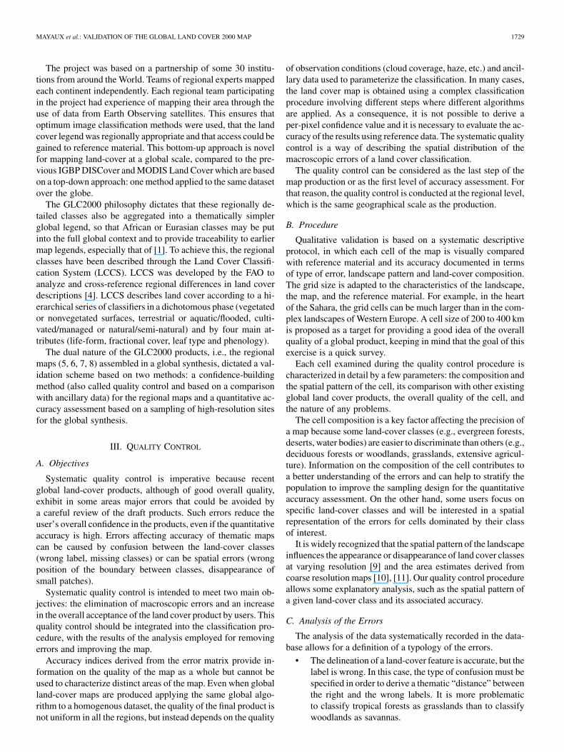
The regional map of Northern Eurasia [5] contains 25 land-cover classes. This map was overlaid by 385 validation cells.We can compute the number of validation cells in which a classis considered as well identified and the number of cells in whichit is poorly identified. Because a validation cell may be coveredby up to five different classes, the total number of occurrences(1554) is higher than the number of validation cells. Table I iden-tifies the classes with low accuracy in this region: needleleafforest (18 to 27% of error) and coniferous shrubs (43%). Notethat a box is covered by up to five different classes, which ex-plains the high number of occurrences.

The label error is the most common (62), with a very limitednumber of errors in the definition of the limits (4), and missingclasses (2). The absence of errors in the limit delineation illus-trates the remarkable geometrical properties of the VEGETA-TION sensor, which allow for recognition of the landscape pat-tern even in the composite images.

Table II shows the interactions between the spatial pattern andthe errors. As expected, most errors are found in heterogeneouslandscapes. Fig. 1 illustrates the utility of the quality controlfor locating the errors on the map. The examination of the spa-tial distribution of errors in an exhaustive way provides to theuser a reliable assessment of the strengths and the caveats of theproduct.

IV. ACCURACY ASSESSMENT

A. Methods

The accuracy assessment of the GLC2000 map has a numberof initial requirements.

1) The assessment should test in priority the main classes ofinterest of the GLC2000 map, i.e., forests, croplands andwetlands.

TABLE ILAND-COVER CELLS CORRECTLY AND BADLY CLASSIFIED ACCORDING

TO THE QUALITY CONTROL IN NORTHERN EURASIA

TABLE IIRELATIONSHIP BETWEEN THE SPATIAL PATTERN AND THE ERRORS

Fig. 1. Errors estimated in Northern Eurasia by the quality control procedure(four increasing levels of error from white to black).

2) To provide a global accuracy of the product, samplingunits should have a worldwide distribution since differentteams have produced the regional products with differentaccuracies.

3) The landscape complexity has a major impact on the mapaccuracy (reference) and should be taken into account forthe sampling and in the accuracy reporting.

4) For cost/efficiency reasons, the validation is derived fromone single sensor dataset, Landsat, and the sampling de-sign is adapted to it.

5) The sampling design should be based on an equal-areaprojection, since the sampling probability of a pixelshould not be biased by its latitude.

MAYAUX et al.: VALIDATION OF THE GLOBAL LAND COVER 2000 MAP 1731

6) To gain additional sampling units at low cost, we shouldinclude clustered sampling in the design.

7) As much as possible, regional experts should interpret thereference data. Most are independent from the “produc-tion” teams.

8) The interpretation key should be flexible and consistentwith the rules used during the map production (Di Gre-gorio and Jansen, 2000).

9) The absolute location error of SPOT VEGETATION isabout 300 m, which means that a validation protocolbased on the analysis of single pixels can include upto 30% of inaccuracy. A single pixel-based is then toosubject to error and we decided on an analysis of pixelblocks of 3 3 km.

1) Sampling Strategy: With all these constraints, we estab-lished a two-stage stratified clustered sampling. The stratifica-tion was based on the proportion of priority classes and on thelandscape complexity. The two-stage clustering was selected forclear advantages of cost [12] and applied on the Landsat WorldReference 2 System (WRS-2). The sampling strategy involvesthe following steps.

1) The WRS-2 grid provides a convenient sampling framefor a sample of Landsat scenes, as it is the case in the cur-rent validation. However, at high latitudes, a WRS-2 basedsampling becomes very complicated due to the overlap be-tween adjacent scenes that can represent 60% at 60 of lat-itude. To take into account this issue, Voronoï polygonsare computed from the WRS-2 centroids in order to as-sign each GLC2000 pixel to one and only one scene. TheVoronoï polygons are used for the sampling procedure.

2) The proportion of the priority classes (forests, wetlandsand croplands) is calculated from the GLC 2000 map ineach polygon. The polygon is flagged as “Priority” assoon as one of the three thresholds is satisfied:forests, croplands, wetlands.

3) The complexity of each polygon is estimated by theShannon index [13], which is a measure of diversity

where is the proportion of the landscape in cover type, and is the number of land cover types observed. The

larger the value of , the more diverse the landscape. TheShannon index of the GLC2000 cells follows a normaldistribution centered on 0.5. The population is then splitin two strata around this average value ( and ).

4) Four strata are defined from the two criteria: homogenouslandscapes in priority land-cover classes ( ),heterogeneous landscapes in priority land-cover classes( ), homogenous landscapes in nonpriorityland-cover classes ( ) and heterogeneous land-scapes in nonpriority land-cover classes ( ),where is the total number of polygons in each stratum.

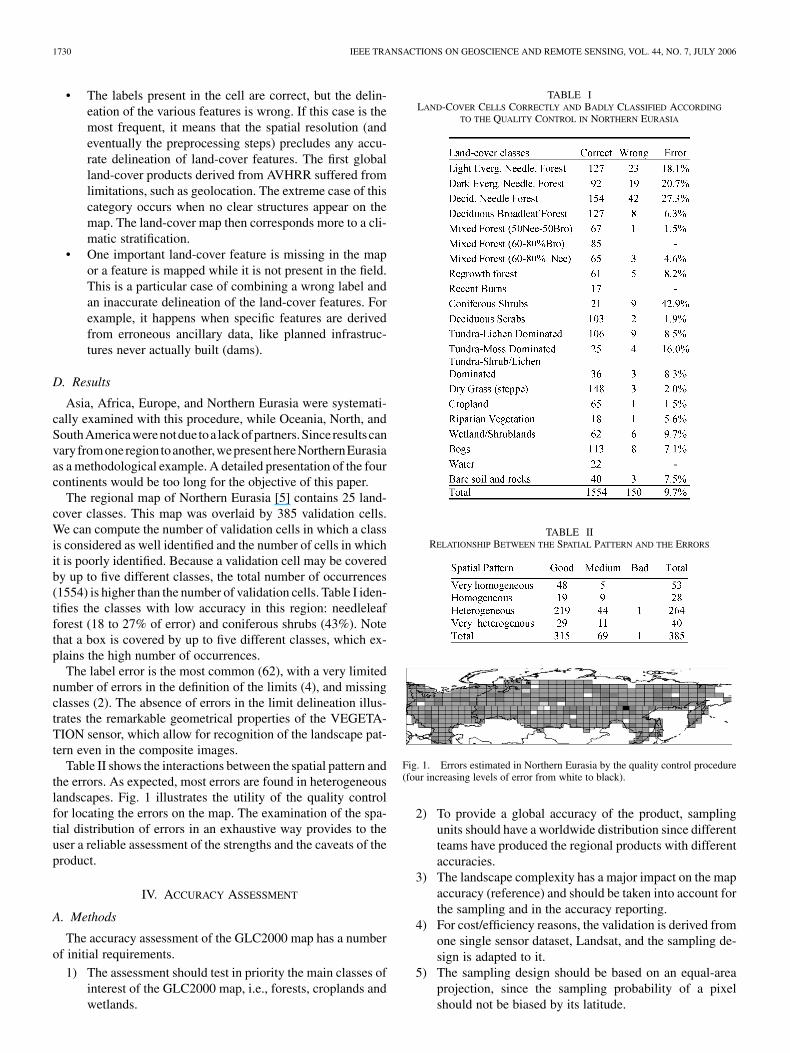
5) A sample grid of blocks (cells of 1800 by 1200km) is overlaid on the GLC2000 map reprojected in anequal-area projection. In each block, six fixed points areselected at a distance of 600 km in the two directions

Fig. 2. Four strata are defined with high to low sampling probabilities. Thesampling rate is as follows: 6/6 (gray), 4/6 (medium gray), 3/6 (light gray), and2/6 (white). The grid of the Voronoï polygons is generated for the globe withequal numbers of each stratum randomly assigned to the polygons. To achievethe sampling rates, a network of points 600 km apart strung over the grid, witheach point being randomly assigned a number from 1 to 6. A polygon is selectedif the number assigned to it is 1 or 2 for the low strata; 1, 2, or 3 for the mediumlow; 1, 2, 3, or 4 for the medium high strata; and 1, 2, 3, 4, 5, or 6 for the highstrata. Hence, in Fig. 3, the point assigned number 4 that falls on the white stratais not selected. Whereas the point 5 that falls on the dark gray strata is selected.

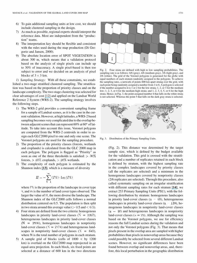
Fig. 3. Distribution of the Primary Sampling Units.

(Fig. 2). This distance was determined by the targetsample size, which is defined by the budget availablefor the validation. This grid is crossed with the stratifi-cation and a number of replicates retained in each blockis defined by stratum, with the highest sampling ratein the complex landscapes covered by priority classes(all the replicates are selected) and a minimum in thehomogenous landscapes covered by nonpriority classes(2/6 replicates are selected). Through this procedure, alsocalled systematic sampling on an irregular stratificationwith different sampling rates for each stratum [14], weextract 253 Primary Sampling Units (PSU), with the fol-lowing distribution by stratum: homogenous landscapesin priority land-cover classes ( ), heterogeneouslandscapes in priority land-cover classes ( ), ho-mogenous landscapes in nonpriority land-cover classes( ) and heterogeneous landscapes in nonpriorityland-cover classes ( ). Although the sampling wasbased on the Voronoï polygons, we use for efficiencyreasons the full Landsat scenes during the validation andnot only the Voronoï polygons (Fig. 3). That means thatpixels present in the overlap area are sampled with higherprobabilities than pixels in nonoverlap areas because theycould possibly be selected from several different Landsatscenes. However, no significant differences have beenfound between overlap and nonoverlap areas, and, there-fore, this local perturbation in the geographic distribution

1732 IEEE TRANSACTIONS ON GEOSCIENCE AND REMOTE SENSING, VOL. 44, NO. 7, JULY 2006

of sampling probability will have a minimal effect onthe ultimate results. If we consider the orbital paths asa systematic sample with a random starting point, inde-pendent of the land cover, the final sampling probabilityis nearly constant within each stratum

where and are the area and sample size (first stage)in stratum , km is the area of each SSU and

is the number of SSU sampled in each SSU.has a slight perturbation in the boundaries between strata.

6) For each Landsat scene, we extract five boxes of 3 3km, the Secondary Sampling Units (SSU), at the centreof the Landsat scene and at each corner of a rectangleof 100 100 km centered on this first box. The pro-cedure avoids sample units (boxes) too close to eachother, reducing the impact of spatial autocorrelationand improving the precision of the accuracy estimates.Boxes were chosen for the interpretation in order to re-duce the misregistration impact. In total, 1,265 SSU areinterpreted.

2) Reference Data: The GLC2000 validation profited fromthe Landsat dataset for the year 2000 sponsored by NASA [15].These Landsat scenes were orthorectified with a nominal accu-racy of 50 meters. Data were downloaded from the Global LandCover Facility (http://glcf.umiacs.umd.edu/index.shtml) or pro-vided by the U.S. Geological Survey. Landsat channels 3, 4, 5,and 7 are used during the interpretation process. For each scene,a quick-look is created at 142.5-m spatial resolution and the SSUare extracted at full resolution. Regional interpreters used ancil-lary data like aerial photographs, thematic maps and NDVI pro-files at coarse resolution in support to the Landsat interpretation.

3) Interpretation of the Reference Material: The analysis ofeach SSU is done by one partner with ecological knowledge ofthe local situation and expertise in fine resolution data interpre-tation. Within one continent, only a few teams were involved inthe procedure for keeping the consistency of the interpretations.

A key challenge of the interpretation protocol is to respectthe logic used during the classification scheme, i.e., a schemebased on objective classifiers that could be aggregated at dif-ferent levels.

Each 3 3 km box is interpreted according to a series ofclassifiers describing the basic parameters of the landscape(vegetated/nonvegetated, natural/artificial, dominant layer),the water conditions (regime, seasonality, quality), detailingthe tree, shrub and grass layers (cover, height, leaf type, andphenology). Some indications are also given on the referencematerial used for supporting the interpretation. When the boxis covered by many spatially distinct land-cover classes, thetwo largest classes are described with the fraction of the boxcovered by each type. A simple interface was developed forstoring the interpretations in a database. Table III details thedifferent fields used for the characterization of the blocks.

Finally, each box is translated to the GLC2000 legend to mea-sure the accuracy of this specific product. This translation wasmade easy by the fact that the classifiers were defined using theGLC2000 classification scheme.

TABLE IIIDETAILED DESCRIPTION OF THE CRITERIA USED IN THE

DATABASE FOR THE INTERPRETATION OF THE BOXES

B. Preliminary Results

The analysis of the interpretations is undertaken using a seriesof tests, designed both to evaluate the validity of the GLC 2000map and to understand better possible causes and the magnitudeof disagreement. The use of pixel boxes as Secondary SamplingUnits, although useful for mitigating for the misregistration ef-fects, made the statistical analysis of the interpretations difficult.Indeed, each box can be covered in the GLC2000 map and in theLandsat interpretation by many land-cover classes. Therefore,we first present the heterogeneity of the blocks. Then, we ex-amine the classical confusion matrix and present an adaptationof the confusion matrix to take into account class similaritiesboth from the producer and from the user point of view.

1) Analysis of Heterogeneity: Due to the different spatialresolutions of the two data sets, we can expect to find many

MAYAUX et al.: VALIDATION OF THE GLOBAL LAND COVER 2000 MAP 1733

Fig. 4. Distribution of blocks according to the proportion of the dominantland-cover in the GLC 2000 map and in the Landsat interpretation. In darkgray, the blocks present a high homogeneity in GLC 2000 and in the Landsatinterpretations.

cases in which the reference data have more than one class com-pared to the map data. We can reasonably expect in the caseof a correct classification that a composite class in the mapdata (e.g., mosaic of forest and agriculture) would correspondto two classes in the reference data. We, therefore, examinedthe number of reference sites that contain single and multipleclasses and compare these to our map data so as to give an ideaas to the magnitude of this problem and what its effect is on theoverall classification accuracy.

From the proportion of the box covered by the dominant land-cover, we can define four situations (Fig. 4).

1) The main land-cover class of each sample (GLC 2000map and Landsat interpretation) covers more than 80%of the box. The cell is then considered as homogenousand is processed as a single point. It represents 544 boxeson a total of 1178, with 300 boxes purely covered by oneclass in the two populations.

2) The box is covered at 80% by one land-cover class inthe GLC 2000 map, but by two classes in the Landsatinterpretation. It means that the map overestimates theproportion of this land-cover class, even in case of correctclassification (commission error). 301 boxes are in thiscase, with 196 covered at 100% by one class.

3) The box is covered by more than one land-cover classin the GLC 2000 map, but by one class in the Landsatinterpretation. It means that the map underestimates theproportion of this land-cover class, even in the case ofcorrect classification (omission error). 146 boxes are inthis case, with 83 covered at 100% by one class.

4) The box is covered by more than one land-cover class inthe GLC 2000 map and in the Landsat interpretation. Thismore complex situation is present in 196 blocks. The onlyway to measure the map accuracy in this case is to workwith fuzzy logic [16].

As a first conclusion, we can say that dataset is very homo-geneous. About 50% of the population is dominated by oneland-cover class in both datasets. At the opposite, the situationmixing different land-cover types in both datasets representsless than 20% of the population.

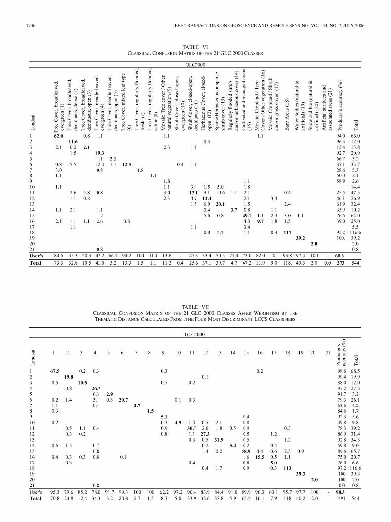
2) Classical Accuracy Metrics: We produced a confusionmatrix [17] for the 21 land cover classes so as to obtain a firstmeasure of overall, the user’s and the producer’s accuracies. Atthis stage, we just give a flavor of the accuracy, taking into ac-count only the 544 blocks dominated by one land-cover class atleast 80%. Table VI details the classical confusion matrix andthe user’s and producer’s accuracy.

We have used a two-stage systematic sampling plan slightlymodified to take into account the geometry of Landsat TMframes. Systematic sampling is generally more efficient thanrandom sampling, but there are no unbiased estimators for thevariance under systematic sampling. We have used classicalformulae for two-stage random sampling [18, Ch. 10], thatover-estimate the variance. Therefore, we give pessimisticvalues for the standard error, although estimators with a smallerbias are possible [19].

For the global accuracy

where is the average proportion of pixels correctly classifiedin stratum , is the proportion of pixels correctlyclassified in PSU ,, is the number of PSU sampled in thestratum, is the average number of boxes sampled in eachPSU, and and are the sampling fractions in the first andsecond sampling stages, and and are the areas for eachstratum and the total area. We obtain a standard error for theaccuracy of 2.6%. This gives a (conservative) 95% confidenceinterval of for the overall accuracy.

The overall GLC2000 (21 classes) accuracy is similar to theIGBP DISCover (17 classes) [20]. We must recognize that theresults expected for the other blocks (with no dominant landcover) should be less favorable. Their analysis is still on-goingthrough methods derived from the fuzzy logic.

3) Adjusted Accuracy Matrices—The Producers Perspec-tive: The heterogeneity analysis leads us to present a set ofadjusted accuracy matrices, where we take into account classsimilarities both from the producer’s point of view and fromthe user’s point of view. These new matrices aim to quantifythe magnitude of the error from different perspectives. In theclassical confusion matrix a misclassification of a desert areaas an evergreen forest has the same impact as classifying asemi-deciduous forest as an evergreen forest. From both aproducer and a user’s point of view, we need to present a matrixwhere misclassifications between similar classes are weightedlower than misclassifications between dissimilar classes. Onwhat basis do we measure “similarity” then?

From the producer’s point of view, two related parametersinfluence the separability between classes: the spectral separa-bility in the dataset and the confusion in the legend definition.As many different regional classification techniques were usedduring the map production [3], it is not possible to measureglobally the spectral separability. For estimating thematic simi-larity from the legend point of view, we measured the proximity

1734 IEEE TRANSACTIONS ON GEOSCIENCE AND REMOTE SENSING, VOL. 44, NO. 7, JULY 2006

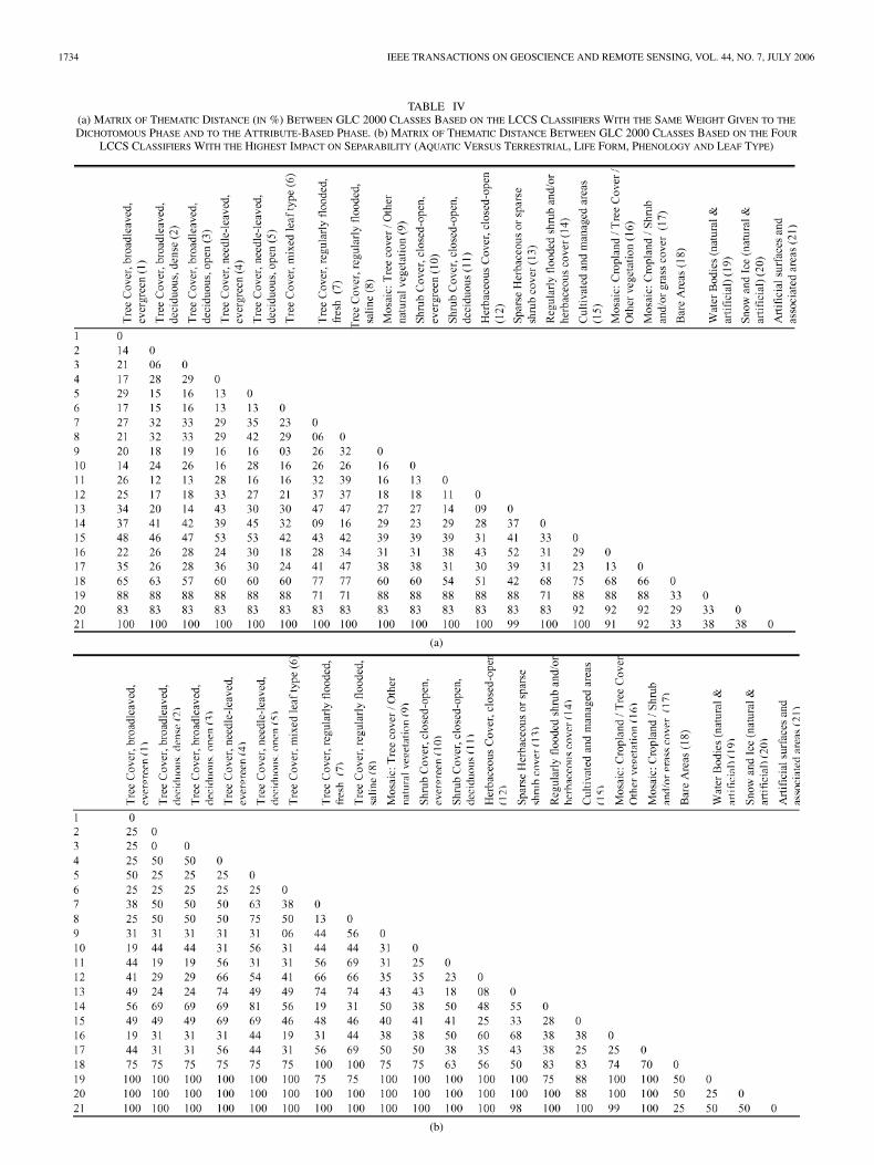
TABLE IV(a) MATRIX OF THEMATIC DISTANCE (IN %) BETWEEN GLC 2000 CLASSES BASED ON THE LCCS CLASSIFIERS WITH THE SAME WEIGHT GIVEN TO THE

DICHOTOMOUS PHASE AND TO THE ATTRIBUTE-BASED PHASE. (b) MATRIX OF THEMATIC DISTANCE BETWEEN GLC 2000 CLASSES BASED ON THE FOUR

LCCS CLASSIFIERS WITH THE HIGHEST IMPACT ON SEPARABILITY (AQUATIC VERSUS TERRESTRIAL, LIFE FORM, PHENOLOGY AND LEAF TYPE)

(a)

(b)

MAYAUX et al.: VALIDATION OF THE GLOBAL LAND COVER 2000 MAP 1735

between classes in the different LCCS classifiers. LCCSscheme combines two classifying phases, one dichotomousat three levels (i.e., a choice between two options—vegetatedOR nonvegetated, artificial OR natural, aquatic OR terrestrial)and the other four based on attributes: life form (trees, shrubs,grasses, bare soil), phenology (evergreen, deciduous, mixed),leaf type (broadleaf, needleleaf, mixed), and vegetation cover(dense, open, sparse, bare). For each of the seven classifierswe developed a similarity matrix showing the correspondencebetween class pairs from 0 to 1. For example, the distance of“Tree cover broadleaved evergreen” in terms of phenology is1 with “Tree cover broadleaved deciduous” and 0.5 with “Treecover Mixed.” The overall similarity is the combination of theseven parameters, ideally with the same weight given to thedichotomous phase and to the attribute-based phase for strictlyrespecting the LCCS approach. However, some classifiers canbe highly correlated, like vegetal versus nonvegetal and the lifeform. Many land-cover classes are characterized by the samedichotomous classifiers and distinct by only one attribute, theiroverall similarity is then very high and it artificially augmentsthe resulting map accuracy. For example, 11 classes covering61% of the land belong to one single category defined duringthe dichotomous phase (vegetal, natural, terrestrial), that meansthat the numerical distance between these classes will reflectonly the differences in the attributes (four classifiers on seven).For accounting for this artifact, we also calculated a similaritymatrix with the four factors giving the best separability, i.e.,aquatic/terrestrial, life form, phenology and leaf type. Table IVshows the similarity matrices with the two methods. The re-sultant matrix is now applied to the original confusion matrixby removing the errors due to thematic proximity in the legenddefinition, and by adding the similarities to the diagonal of thematrix.

If we call the confusion matrix, the global accuracy can bewritten

whereifif

is the “sharp” thematic distance.

If is substituted by the fuzzy thematic distance given inTable IV, we get the fuzzy global accuracy

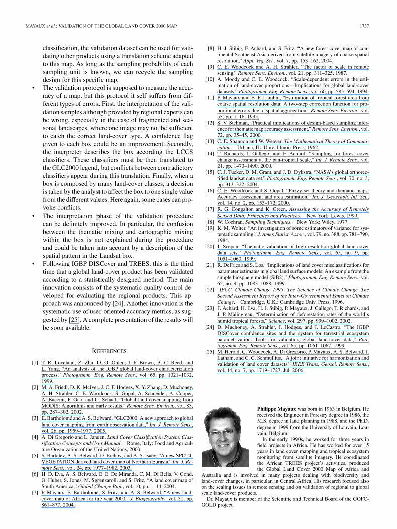
In Table VII, we show the example of the confusion matrixadjusted by the similarity matrix computed from the four fac-tors giving the best separability. The overall accuracy is now90.3% between the 21 classes, with a very drastic improvementfor the accuracy of the mosaic classes, and 92.6% with the simi-larity matrix weighting in the same way the dichotomous phaseand the attribute-based phase. A similar approach was devel-oped for the IGBP DISCover dataset, calculating the similarityof land-cover classes according to their Leaf Area Index and

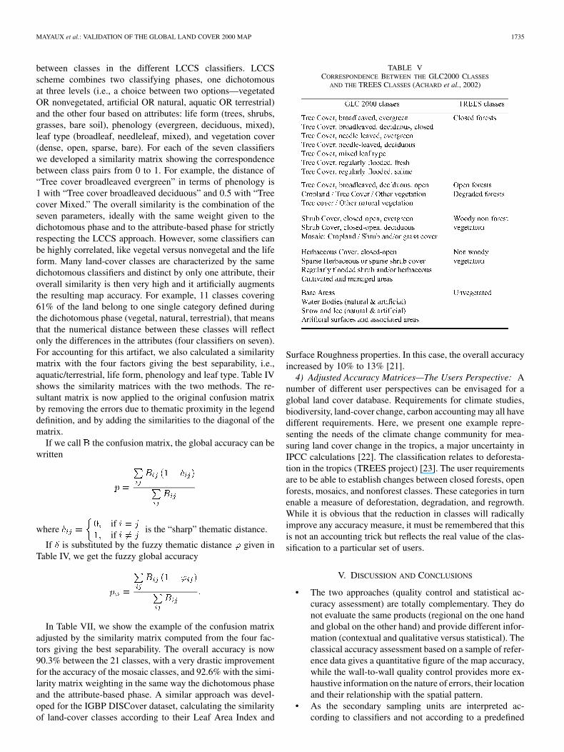
TABLE VCORRESPONDENCE BETWEEN THE GLC2000 CLASSES

AND THE TREES CLASSES (ACHARD et al., 2002)

Surface Roughness properties. In this case, the overall accuracyincreased by 10% to 13% [21].

4) Adjusted Accuracy Matrices—The Users Perspective: Anumber of different user perspectives can be envisaged for aglobal land cover database. Requirements for climate studies,biodiversity, land-cover change, carbon accounting may all havedifferent requirements. Here, we present one example repre-senting the needs of the climate change community for mea-suring land cover change in the tropics, a major uncertainty inIPCC calculations [22]. The classification relates to deforesta-tion in the tropics (TREES project) [23]. The user requirementsare to be able to establish changes between closed forests, openforests, mosaics, and nonforest classes. These categories in turnenable a measure of deforestation, degradation, and regrowth.While it is obvious that the reduction in classes will radicallyimprove any accuracy measure, it must be remembered that thisis not an accounting trick but reflects the real value of the clas-sification to a particular set of users.

V. DISCUSSION AND CONCLUSIONS

• The two approaches (quality control and statistical ac-curacy assessment) are totally complementary. They donot evaluate the same products (regional on the one handand global on the other hand) and provide different infor-mation (contextual and qualitative versus statistical). Theclassical accuracy assessment based on a sample of refer-ence data gives a quantitative figure of the map accuracy,while the wall-to-wall quality control provides more ex-haustive information on the nature of errors, their locationand their relationship with the spatial pattern.

• As the secondary sampling units are interpreted ac-cording to classifiers and not according to a predefined

1736 IEEE TRANSACTIONS ON GEOSCIENCE AND REMOTE SENSING, VOL. 44, NO. 7, JULY 2006

TABLE VICLASSICAL CONFUSION MATRIX OF THE 21 GLC 2000 CLASSES

TABLE VIICLASSICAL CONFUSION MATRIX OF THE 21 GLC 2000 CLASSES AFTER WEIGHTING BY THE

THEMATIC DISTANCE CALCULATED FROM .THE FOUR MOST DISCRIMINANT LCCS CLASSIFIERS

MAYAUX et al.: VALIDATION OF THE GLOBAL LAND COVER 2000 MAP 1737

classification, the validation dataset can be used for vali-dating other products using a translation scheme adaptedto this map. As long as the sampling probability of eachsampling unit is known, we can recycle the samplingdesign for this specific map.

• The validation protocol is supposed to measure the accu-racy of a map, but this protocol it self suffers from dif-ferent types of errors. First, the interpretation of the vali-dation samples although provided by regional experts canbe wrong, especially in the case of fragmented and sea-sonal landscapes, where one image may not be sufficientto catch the correct land-cover type. A confidence flaggiven to each box could be an improvement. Secondly,the interpreter describes the box according the LCCSclassifiers. These classifiers must be then translated tothe GLC2000 legend, but conflicts between contradictoryclassifiers appear during this translation. Finally, when abox is composed by many land-cover classes, a decisionis taken by the analyst to affect the box to one single valuefrom the different values. Here again, some cases can pro-voke conflicts.

• The interpretation phase of the validation procedurecan be definitely improved. In particular, the confusionbetween the thematic mixing and cartographic mixingwithin the box is not explained during the procedureand could be taken into account by a description of thespatial pattern in the Landsat box.

• Following IGBP DISCover and TREES, this is the thirdtime that a global land-cover product has been validatedaccording to a statistically designed method. The maininnovation consists of the systematic quality control de-veloped for evaluating the regional products. This ap-proach was announced by [24]. Another innovation is thesystematic use of user-oriented accuracy metrics, as sug-gested by [25]. A complete presentation of the results willbe soon available.

REFERENCES

[1] T. R. Loveland, Z. Zhu, D. O. Ohlen, J. F. Brown, B. C. Reed, andL. Yang, “An analysis of the IGBP global land-cover characterizationprocess,” Photogramm. Eng. Remote Sens., vol. 65, pp. 1021–1032,1999.

[2] M. A. Friedl, D. K. McIver, J. C. F. Hodges, X. Y. Zhang, D. Muchoney,A. H. Strahler, C. E. Woodcock, S. Gopal, A. Schneider, A. Cooper,A. Baccini, F. Gao, and C. Schaaf, “Global land cover mapping fromMODIS: Algorithms and early results,” Remote Sens. Environ., vol. 83,pp. 287–302, 2002.

[3] E. Bartholomé and A. S. Belward, “GLC2000: A new approach to globalland cover mapping from earth observation data,” Int. J. Remote Sens.,vol. 26, pp. 1959–1977, 2005.

[4] A. Di Gregorio and L. Jansen, Land Cover Classification System, Clas-sification Concepts and User Manual. Rome, Italy: Food and Agricul-ture Organization of the United Nations, 2000.

[5] S. Bartalev, A. S. Belward, D. Erchov, and A. S. Isaev, “A new SPOT4-VEGETATION derived land cover map of Northern Eurasia,” Int. J. Re-mote Sens., vol. 24, pp. 1977–1982, 2003.

[6] H. D. Eva, A. S. Belward, E. E. De Miranda, C. M. Di Bella, V. Gond,O. Huber, S. Jones, M. Sgrenzaroli, and S. Fritz, “A land cover map ofSouth America,” Global Change Biol., vol. 10, pp. 1–14, 2004.

[7] P. Mayaux, E. Bartholomé, S. Fritz, and A. S. Belward, “A new land-cover map of Africa for the year 2000,” J. Biogeography, vol. 31, pp.861–877, 2004.

[8] H.-J. Stibig, F. Achard, and S. Fritz, “A new forest cover map of con-tinental Southeast Asia derived from satellite imagery of coarse spatialresolution,” Appl. Veg. Sci., vol. 7, pp. 153–162, 2004.

[9] C. E. Woodcock and A. H. Strahler, “The factor of scale in remotesensing,” Remote Sens. Environ., vol. 21, pp. 311–325, 1987.

[10] A. Moody and C. E. Woodcock, “Scale-dependent errors in the esti-mation of land-cover proportions—Implications for global land-coverdatasets,” Photogramm. Eng. Remote Sens., vol. 60, pp. 585–594, 1994.

[11] P. Mayaux and E. F. Lambin, “Estimation of tropical forest area fromcoarse spatial resolution data: A two-step correction function for pro-portional errors due to spatial aggregation,” Remote Sens. Environ., vol.53, pp. 1–16, 1995.

[12] S. V. Stehman, “Practical implications of design-based sampling infer-ence for thematic map accuracy assessment,” Remote Sens. Environ., vol.72, pp. 35–45, 2000.

[13] C. E. Shannon and W. Weaver, The Mathematical Theory of Communi-cation. Urbana, IL: Univ. Illinois Press, 1962.

[14] T. Richards, J. Gallego, and F. Achard, “Sampling for forest coverchange assessment at the pan-tropical scale,” Int. J. Remote Sens., vol.21, pp. 1473–1490, 2000.

[15] C. J. Tucker, D. M. Grant, and J. D. Dykstra, “NASA’s global orthorec-tified landsat data set,” Photogramm. Eng. Remote Sens., vol. 70, no. 3,pp. 313–322, 2004.

[16] C. E. Woodcock and S. Gopal, “Fuzzy set theory and thematic maps:Accuracy assessment and area estimation,” Int. J. Geograph. Inf. Sci.,vol. 14, no. 2, pp. 153–172, 2000.

[17] R. G. Congalton and K. Green, Assessing the Accuracy of RemotelySensed Data; Principles and Practices. New York: Lewis, 1999.

[18] W. Cochran, Sampling Techniques. New York: Wiley, 1977.[19] K. M. Wolter, “An investigation of some estimators of variance for sys-

tematic sampling,” J. Amer. Statist. Assoc., vol. 79, no. 388, pp. 781–790,1984.

[20] J. Scepan, “Thematic validation of high-resolution global land-coverdata sets,” Photogramm. Eng. Remote Sens., vol. 65, no. 9, pp.1051–1060, 1999.

[21] R. DeFries and S. Los, “Implications of land cover misclassifications forparameter estimates in global land surface models: An example from thesimple biosphere model (SiB2),” Photogramm. Eng. Remote Sens., vol.65, no. 9, pp. 1083–1088, 1999.

[22] IPCC, Climate Change 1995- The Science of Climate Change. TheSecond Assessment Report of the Inter-Governmental Panel on ClimateChange. Cambridge, U.K.: Cambridge Univ. Press, 1996.

[23] F. Achard, H. Eva, H. J. Stibig, P. Mayaux, J. Gallego, T. Richards, andJ. P. Malingreau, “Determination of deforestation rates of the world’shumid tropical forests,” Science, vol. 297, pp. 999–1002, 2002.

[24] D. Muchoney, A. Strahler, J. Hodges, and J. LoCastro, “The IGBPDISCover confidence sites and the system for terrestrial ecosystemparametrization: Tools for validating global land-cover data,” Pho-togramm. Eng. Remote Sens., vol. 65, pp. 1061–1067, 1999.

[25] M. Herold, C. Woodcock, A. Di Gregorio, P. Mayaux, A. S. Belward, J.Latham, and C. C. Schmullius, “A joint initiative for harmonization andvalidation of land cover datasets,” IEEE Trans. Geosci. Remote Sens.,vol. 44, no. 7, pp. 1719–1727, Jul. 2006.

Philippe Mayaux was born in 1963 in Belgium. Hereceived the Engineer in Forestry degree in 1986, theM.S. degree in land planning in 1988, and the Ph.D.degree in 1999 from the University of Louvain, Lou-vain, Belgium.

In the early 1990s, he worked for three years infield projects in Africa. He has worked for over 15years in land cover mapping and tropical ecosystemmonitoring from satellite imagery. He coordinatedthe African TREES project’s activities, producedthe Global Land Cover 2000 Map of Africa and

Australia and is involved in many projects dealing with biodiversity andland-cover changes, in particular, in Central Africa. His research focused alsoon the scaling issues in remote sensing and on validation of regional to globalscale land-cover products.

Dr. Mayaux is member of the Scientific and Technical Board of the GOFC-GOLD project.

1738 IEEE TRANSACTIONS ON GEOSCIENCE AND REMOTE SENSING, VOL. 44, NO. 7, JULY 2006

Hugh Eva was born in 1958 in the U.K. He receivedthe B.Sc. degree from Manchester University, U.K.,the M.Sc. degree from Cranfield University, U.K.,and the Ph.D. degree from the University of Louvain,Louvain, Belgium.

He specialized in the use of remotely sensed datafor mapping fires and forests in tropical ecosystemsand has published two land cover maps of SouthAmerica derived from satellite imagery. He has beenthe Latin America coordinator of the TREES project,which was set up to monitor and measure changes in

the tropical forest belt, using remote sensing.

Javier Gallego was born in 1953 in Spain. He grad-uated with a degree in mathematics in 1975 and thePh.D. degree in statistics in 1979 from the Univer-sity of Valladolid, Valladolid, Spain, and received theDoctorat de troisième cycle from the University ofParis VI, Paris, France, in 1982.

In 1983, he became Head of the Department of Sta-tistics in the University of Valladolid, then Full pro-fessor in 1986. In 1987, he joined the European Com-mission, first in DG Agriculture, and then, in 1988,he joined the European Commission’s Joint Research

Centre, Ispra, Italy, where he has worked on the use of remote sensing forland cover and agricultural statistics (MARS Project), geographic sampling, anddownscaling techniques.

Alan H. Strahler (M’86) received the B.A. andPh.D. degrees in geography from The Johns HopkinsUniversity, Baltimore, MD, in 1964 and 1969,respectively.

He is currently a Professor of geography and a Re-searcher in the Center for Remote Sensing, BostonUniversity, Boston, MA. He has held prior academicpositions at Hunter College, City University of NewYork; University of California, Santa Barbara; andthe University of Virginia, Charlottesville. Originallytrained as a Biogeographer, he has been actively in-

volved in remote-sensing research since 1978. He has been a Principal Investi-gator on numerous NASA contracts and grants. His primary research interestsare directed toward modeling the bidirectional reflectance distribution function(BRDF) of discontinuous vegetation covers and retrieving physical parametersdescribing ground scenes through inversion of BRDF models using directionalradiance measurements. He is also interested in the problem of land cover clas-sification using multitemporal, multispectral, multidirectional, and spatial infor-mation as acquired in reflective and emissive imagery of the earth’s surface.

Dr. Strahler was awarded the AAG/RSSG Medal for Outstanding Contribu-tions to Remote Sensing in 1993 and the honorary degree Doctorem ScientarumHonoris Causa from the Université Catholique du Louvain, Belgium, in 2000.He was also honored as a Fellow of the American Association for the Advance-ment of Science in 2003.

Martin Herold (S’98) was born in Leipzig, Ger-many, in 1975. He received the the graduate degree(Diplom in Geography) from the Friedrich SchillerUniversity of Jena, Jena, Germany, and the BauhausUniversity of Weimar, Weimar, Germany, in 2000,and the Ph.D. degree from the Department of Ge-ography, University of California, Santa Barbara, in2004.

He is currently coordinating the ESA GOFCGOLD Land Cover project office at the FriedrichSchiller University Jena. Earlier in his career, his

interests were in multifrequency, polarimetric and interferometric SAR-dataanalysis for land surface parameter derivation, and modeling. He joined theRemote Sensing Research Unit, University of California Santa Barbara, in2000, where his research has focused on the remote sensing of urban areas andthe analysis and modeling of urban growth and land use change processes. Hismost recent interests are in international coordination and cooperation towardoperational terrestrial observations with specific emphasis on the harmonizationand validation of land cover datasets.

Dr. Herold is a member the German Society of Photogrammetry and RemoteSensing (DGPF) and the Thuringian Geographical Union (TGG).

Shefali Agrawal was born in India. She received thedegree in physics, the M.S. degree in physics, and thePG Diploma in computer management and receivedan Advance Diploma in Geoinformatics from ITC,The Netherlands.

She joined the Indian Institute of Remore Sensing,Dehradun, in 1992, and, since then, she has beenworking in the field of image processing andGIS-based modeling related to land use/land covercharacterization. She contributed to the GLC map ofSouth Central Asia and its validation, as well as the

TREES-II project (for Indian region), sponsored by the European Commission.

Sergey Naumov was born in 1977 in Russia. Hegraduated as a Research Engineer in GIS in 1999 andreceived the Ph.D. degree from the Moscow StateUniversity of Geodesy and Cartography, Moscow,Russia, in 2002.

After graduation, he worked for a Russian satel-lite imagery provider as a specialist for imageryprocessing and three-dimensional modeling ofurban areas. For the past three years, he has beenworking with the Remote Sensing Data ProcessingDepartment, DATA+, Moscow, as a GIS and Remote

Sensing Specialist.

Evaristo Eduardo de Miranda was born in 1952in São Paulo, Brazil. He graduated from the “Insti-tute Superieur d’Agriculture Rhône Alpes” in Lyon,France, and received the M.Sc. and Ph.D. degrees inecology from the University of Montpellier, France,in 1980.

In his professional career, he has been workingwith rural development issues, linking environmentalprotection to agricultural production and satellitemonitoring. He was a UN Consultant for the WorldEnvironmental Summit, Rio de Janeiro, Brazil,

in 1992, and he is a Consultant for organizations such as FAO, UNESCO,FAPESP, World Bank, AEO, and other national and international researchorganizations. He has published hundreds of technical and scientific papers inBrazil, as well as abroad. He is a teacher and advisor for the University of SãoPaulo, São Paulo, Brazil, and at the State University of Campinas, Campinas,Brazil.

MAYAUX et al.: VALIDATION OF THE GLOBAL LAND COVER 2000 MAP 1739

Carlos M. Di Bella was born in Argentina. Hegraduated as an Agronomist from the University ofBuenos Aires, Buenos Aires, Argentina, in 1994, andreceived the Ph.D. degree from the Institut NationalAgronomique Paris-Grignon, France, in 2002.

Since 1998, he has been a Staff Researcher at theInstitute of Climate and Water, Buenos Aires. His re-search focuses on the application and developmentof remote-sensing and GIS techniques to natural re-sources management and monitoring.

Callan Ordoyne received the B.A. degree in bio-logical sciences from Mount Holyoke Colleg, SouthHadley, MA, in 2003. She is currently pursuing theM.S. degree, for which she is studying the remotesensing of wetlands, tracking the annual hydrologicalpattern of the Florida Everglades, Boston University,Boston, MA.

Her undergraduate field was ecology, with a re-search focus on wetland ecology and arachnology. AtBoston University, she worked on the MODIS GlobalLand Cover project, with the primary responsibility

for developing and updating the System for Terrestrial Ecosystem Parameteri-zation database of training sites.

Yuri Kopin was born in 1981 in Russia. He receivedthe B.S. degree in cartography from the LomonosovMoscow State University, Mosow, Russia, in 2002.

His main activities include land cover classifica-tion, remote sensing in cadastre, and radar mapping.

P. S. Roy received the M.S. degree in botany in 1973and the Ph.D. degree in ecology in 1980.

He is the Deputy Director (RS and GIS–AA)National Remote Sensing Agency, Department ofSpace, Government of India, Hyderabad, India.He specializes in Geoinformatics for EcosystemAnalysis. Presently, he is leading a national forumon Biodiversity Characterization at Landscape Leveland Land Use Land Cover in different scales.