Mapping-of-land-cover-and-estimation-of-their-emissivity ...

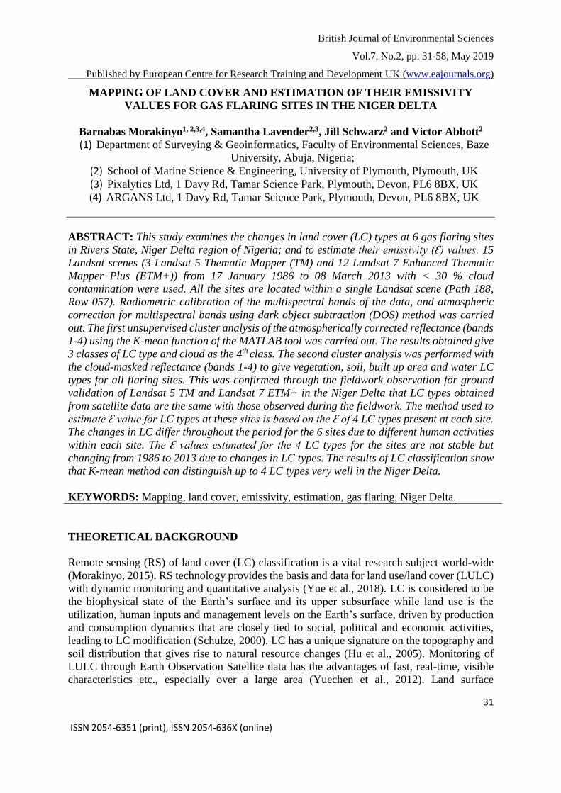
British Journal of Environmental Sciences

Vol.7, No.2, pp. 31-58, May 2019

Published by European Centre for Research Training and Development UK (www.eajournals.org)

31 ISSN 2054-6351 (print), ISSN 2054-636X (online)

MAPPING OF LAND COVER AND ESTIMATION OF THEIR EMISSIVITY

VALUES FOR GAS FLARING SITES IN THE NIGER DELTA

Barnabas Morakinyo1, 2,3,4, Samantha Lavender2,3, Jill Schwarz2 and Victor Abbott2

(1) Department of Surveying & Geoinformatics, Faculty of Environmental Sciences, Baze

University, Abuja, Nigeria;

(2) School of Marine Science & Engineering, University of Plymouth, Plymouth, UK

(3) Pixalytics Ltd, 1 Davy Rd, Tamar Science Park, Plymouth, Devon, PL6 8BX, UK

(4) ARGANS Ltd, 1 Davy Rd, Tamar Science Park, Plymouth, Devon, PL6 8BX, UK

ABSTRACT: This study examines the changes in land cover (LC) types at 6 gas flaring sites

in Rivers State, Niger Delta region of Nigeria; and to estimate their emissivity (Ɛ) values. 15

Landsat scenes (3 Landsat 5 Thematic Mapper (TM) and 12 Landsat 7 Enhanced Thematic

Mapper Plus (ETM+)) from 17 January 1986 to 08 March 2013 with < 30 % cloud

contamination were used. All the sites are located within a single Landsat scene (Path 188,

Row 057). Radiometric calibration of the multispectral bands of the data, and atmospheric

correction for multispectral bands using dark object subtraction (DOS) method was carried

out. The first unsupervised cluster analysis of the atmospherically corrected reflectance (bands

1-4) using the K-mean function of the MATLAB tool was carried out. The results obtained give

3 classes of LC type and cloud as the 4th class. The second cluster analysis was performed with

the cloud-masked reflectance (bands 1-4) to give vegetation, soil, built up area and water LC

types for all flaring sites. This was confirmed through the fieldwork observation for ground

validation of Landsat 5 TM and Landsat 7 ETM+ in the Niger Delta that LC types obtained

from satellite data are the same with those observed during the fieldwork. The method used to

estimate Ɛ value for LC types at these sites is based on the Ɛ of 4 LC types present at each site.

The changes in LC differ throughout the period for the 6 sites due to different human activities

within each site. The Ɛ values estimated for the 4 LC types for the sites are not stable but

changing from 1986 to 2013 due to changes in LC types. The results of LC classification show

that K-mean method can distinguish up to 4 LC types very well in the Niger Delta.

KEYWORDS: Mapping, land cover, emissivity, estimation, gas flaring, Niger Delta.

THEORETICAL BACKGROUND

Remote sensing (RS) of land cover (LC) classification is a vital research subject world-wide

(Morakinyo, 2015). RS technology provides the basis and data for land use/land cover (LULC)

with dynamic monitoring and quantitative analysis (Yue et al., 2018). LC is considered to be

the biophysical state of the Earth’s surface and its upper subsurface while land use is the

utilization, human inputs and management levels on the Earth’s surface, driven by production

and consumption dynamics that are closely tied to social, political and economic activities,

leading to LC modification (Schulze, 2000). LC has a unique signature on the topography and

soil distribution that gives rise to natural resource changes (Hu et al., 2005). Monitoring of

LULC through Earth Observation Satellite data has the advantages of fast, real-time, visible

characteristics etc., especially over a large area (Yuechen et al., 2012). Land surface

http://www.eajournals.org/


Vol.7, No.2, pp. 31-58, May 2019



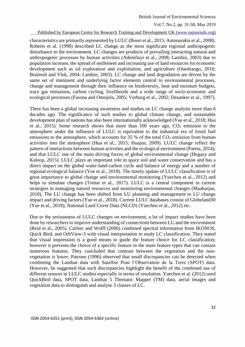
characteristics are primarily represented by LULC (Boori et al., 2015; Antonarakis et al., 2008).

Roberts et al. (1998) described LC change as the most significant regional anthropogenic

disturbance to the environment. LC changes are products of prevailing interacting natural and

anthropogenic processes by human activities (Ademiluyi et al., 2008; Lambin, 2003) due to

population increase, the spread of settlement and increasing use of land resources for economic

development such as oil exploration and exploitation, and agriculture (Ouedraogo, 2010;

Braimoh and Vlek, 2004; Lambin, 2003). LC change and land degradation are driven by the

same set of imminent and underlying factor elements central to environmental processes,

change and management through their influence on biodiversity, heat and moisture budgets,

trace gas emissions, carbon cycling, livelihoods and a wide range of socio-economic and

ecological processes (Fasona and Omojola, 2005; Verburg et al., 2002; Desanker et al., 1997).

There has been a global increasing awareness and studies on LC change analysis more than 6

decades ago. The significance of such studies to global climate change, and sustainable

development plan of nations has also been internationally acknowledged (Yue et al., 2018; Hua

et al., 2015). Some research shows that more than 100 years ago, CO2 emission to the

atmosphere under the influence of LULC is equivalent to the industrial era of fossil fuel

emissions to the atmosphere, which accounts for 35 % of the total CO2 emission from human

activities into the atmosphere (Hua et al., 2015; Huajun, 2009). LULC change reflect the

pattern of interactions between human activities and the ecological environment (Pareta, 2014);

and that LULC one of the main driving forces of global environmental change (Hegazy and

Kaloop, 2015). LULC plays an important role in space soil and water conservation and has a

direct impact on the global water-land-carbon cycle and balance of energy and a number of

regional ecological balance (Yue et al., 2018). The timely update of LULC classification is of

great importance to global change and environmental monitoring (Yuechen et al., 2012) and

helps to simulate changes (Tomar et al., 2017). LULC is a central component in current

strategies in managing natural resources and monitoring environmental changes (Maaharjan,

2018). The LU change has been shifted from LU planning and management to LU change

impact and driving factors (Yue et al., 2018). Current LULC databases consist of Globeland30

(Yue et al., 2018); National Land Cover Data (NLCD) (Yuechen et al., 2012) etc.

Due to the seriousness of LULC changes on environment, a lot of impact studies have been

done by researchers to improve understanding of connections between LU and the environment

(Reid et al., 2005). Carleer and Wolff (2006) combined spectral information from IKONOS,

Quick Bird, and OrbView-3 with visual interpretation to study LC classification. They stated

that visual impression is a good means to guide the feature choice for LC classification;

however it prevents the choice of a specific feature in the main feature types that can contain

numerous features. They concluded that contrast between the vegetation and the non-

vegetation is lower. Patrono (1996) observed that small discrepancies can be detected when

combining the Landsat data with Satellite Pour l’Observation de la Terre (SPOT) data.

However, he suggested that such discrepancies highlight the benefit of the combined use of

different sensors in LULC studies especially in terms of resolution. Yuechen et al. (2012) used

QuickBird data, SPOT data, Landsat 5 Thematic Mapper (TM) data, aerial images and

vegetation data to distinguish and analyse 3 classes of LC.



Vol.7, No.2, pp. 31-58, May 2019



In addition, Gong et al. (2006) combined airborne remote sensing data and ground survey data

for LULC studies and analysis. Aixia et al. (2006) used MODerate Resolution Imaging

Spectroradiometer (MODIS) data, Landsat 7 Enhanced Thematic Mapper Plus (ETM+) data,

and Land Surface Temperature (LST) and Normalized Difference Vegetation Index (NDVI)

time series datasets for LC classification. Advanced Spaceborne Thermal Emission and

Reflection Radiometer (ASTER) data of 2003 with a spatial resolution of 15 m was employed

by Rahman et al. (2012) for analysis of LC change. Maaharjan (2018) employed Landsat 8

Operational Land Imager (OLI) and Thermal Infrared Sensor (TIRS) C1 Level-1 and Landsat

5 TM C1 level -1 for LC classification. Fonteh et al. (2016) investigated, compared and

integrated the use of Sentinel-1 C band Synthetic Aperture Radar (SAR) and Landsat 7 ETM+

for extracting LULC information in the coastal area. They stated that Sentinel-1 only, yielded

a lower overall classification accuracy of 67.65 % when compared to all Landsat 7 ETM+

bands of 88.7 %. The integrated Sentinel-1 and Landsat 7 ETM+ showed no significant

differences in overall accuracy assessment of 88.71 % and 88.59 % respectively. The 3 best

spectral bands (5, 6, 7) of Landsat imagery yielded the highest overall accuracy assessment of

91.96 %. These results demonstrate a lower potential of Sentinel-1 for LC in the humid

environment when compared with cloud free Landsat images (Fonteh et al., 2016). Textural

variables including mean, correlation, contrast and entropy were derived from the Sentinel-1 C

band (Fonteh et al., 2016). Yeboah et al. (2017) and Pareta (2014) acquired Landsat 5 TM,

Landsat ETM+, field data and Google Earth imagery (Tomar et al., 2017) for LULC studies

and change detection; Braimoh and Vlek (2004) undertook LULC in the Volta Basin part of

Ghana; and Forkuo and Adubofour (2012) quantified the forest cover change patterns in the

Owabi area in the Ashanti Region of Ghana and demonstrated the potential of multi-temporal

satellite data to map and analyse changes in LC in spatio-temporal framework.

In Nigeria, few researchers on LULC studies includes Nnaji et al. (2016) who carried out spatio

temporal analysis of LULC changes in Owerri Municipal and its environs, Imo State, using

Landsat 7 ETM+ of 1991, 2001 and 2014. They distinguished 6 classes of LC (built-up area,

open space, forest, farmland, vegetation and water bodies). They concluded that the rate of

change shows that built up area was on continuous increase and open space was on a continuous

decrease throughout the study period. Awoniran et al., (2013) investigated LULC change of

the lower Ogun River Basin between 1984 and 2012 using a Landsat 5 TM data (1984), Landsat

7 ETM+ data (2000), and a Google Earth image of 2012. The result shows that between 1984

and 2000, 80.08 % of the LC in the study area has been converted to other LU while only 19.92

% remained unchanged. Also, Tokula and Ejaro (2012) used Landsat 7 ETM+ (1987); Landsat

5 TM (2001) and (2011) for the classification of agriculture land, bare soil, vegetation, and

built up LC types. They concluded that most of agriculture land and vegetation were converted

to built up areas.

Furthermore, Agoha (2009), analysed rural-urban LU change in Umuahia, Abia State, between

1991 and 2007 and observed that builtup area increased over the study period while agricultural

land and vegetation depreciated significantly. Similarly, Ejaro, (2008) undertook analysis of

LULC change in the Federal Capital Territory (FCT), Abuja, using Landsat data from 1973 to

2006. The results show that the proportion of area covered by built up land and bare surface

was on increase while there is an alarming decline in vegetation and agricultural land. He stated

that the geographical location, political and socio-economic activities and importance of the



Vol.7, No.2, pp. 31-58, May 2019



FCT, which cause the rapid growth of human population and expansion, are the major reasons

that have greatly influenced the changes in LULC in the FCT, Abuja especially reducing

vegetation cover. Olowolafe et al. (2010) and Idowu and Muazu (2010) studied LULC and

change detection; they found that agricultural land increased by 2.18 km2 (28.17 %). They

attributed the increase in agricultural land to the adoption of new agricultural practices which

made some un-usable land before 2008 usable due to provision of agricultural incentives such

as fertilizers supplies and irrigation by Katsina State Government.

However, there is still a low level of recognition and research attention on LC types studies in

Nigeria (Okude, 2006). Only a small number of studies on mapping of LULC have been

undertaken in Nigeria despite the increasing worldwide (Ademiluyi et al, 2008). The diversity

is decreasing and the need to balance human well-being and environmental sustainability

involves adjusting the way the ecosystem goods and services produced by the land are used.

According to Ringrose et al. (1997), LULC change in Africa is currently accelerating and

causing widespread environmental problems and thus needs to be mapped. This is important

because the changing patterns of LULC reflect changing economic and social conditions.

Monitoring such changes is important for coordinated actions at the national and international

levels (Bernard and Wilkinson, 1997). At present, some problems in LULC change research

can be grouped as: (a) Insufficient data from other land surveying methods except remote

sensing data which is influenced by weather, precision of equipment, etc. (b) Most of the LULC

models are greatly affected by the regional environmental factors, causing the function of the

established models not to be well represented globally due to the limitation of data quality. (c)

There is no unified theoretical system for reference, so the methods and models used by

researchers have obvious regional limitations (Yue et al., 2018).

Emissivity (Ɛ) is the ratio of energy emitted from a natural material to that from an ideal

blackbody at the same temperature (Mallick et al., 2012). An accurate value of surface Ɛ is

desired in land surface models for better simulations of surface energy budgets from which

skin temperature is calculated (Jin et al., 1997). The Ɛ of natural land surface is determined by

soil structure, soil composition, organic matter, moisture content, and vegetation cover

characteristics (Van de Griend and Owe, 1993). The Ɛ value always lies between 0 and 1 (Jin

and Liang, 2006). The knowledge of surface Ɛ is important for estimating the land surface

temperature (LST). It can reduce the error in estimating the surface temperature from thermal

satellite data. Remotely sensing a surface Ɛ is very challenging because of the high

heterogeneity of land surfaces and the difficulties in removing atmospheric effects (Liang,

2004; Liang, 2001; Wan and Li, 1997). Current Ɛ databases consist of MODIS, ASTER and

Landsat products (Mallick et al., 2012).

Researchers have worked on Ɛ, for example Pu et al. (2006) used a constant value of Ɛ= 1 for

all materials, although the authors stated that it is not a wise decision. Peng et al. (2008) and

Xu et al. (2008) retrieved spectral Ɛ over urban areas in a pixel-by-pixel basis. Furthermore,

many studies have been carried out in order to retrieve land surface Ɛ, such as temperature-

independent spectral indices (TISI) methods (Zhu, 2006; Becker and Li, 1995; Li and Becker,

1993). This algorithm combines middle wave infrared data (MWIR: 3.4-5.2 µm) with thermal

infrared data (TIR: 8-14 µm) to estimate Ɛ. Gillespie et al. (1998) developed this method for

ASTER data and estimated Ɛ with high accuracy. However, the accuracy of this algorithm



Vol.7, No.2, pp. 31-58, May 2019



depends on some assumptions and ties to the atmospheric correction. NDVI methods proposed

by Caselles and Sobrino (1989) and developed by van de Griend and Owe (1993) supplied a

technique to calculate Ɛ, and its successful performance in natural surface. But this method was

based on the assumption that the land surface is mainly made up of vegetations and soil, which

is not in agreement with land surface. Jimenez-Munoz et al. (2006) used NDVI based Ɛ method

to obtain surface Ɛs over agricultural areas from ASTER data, and found that band 13 gave

most accurate Ɛ measurement. Wan and Dozier (1996) utilized a classification-based Ɛ method

and applied results to split window method, which performed satisfactorily. Snyder et al.

(1998) also used this method to retrieve global Ɛ without considering the complicated urban

surface heterogeneous.

Emissivity has strong seasonality and LULC dependence (Mallick et al., 2012). Specifically, Ɛ

depends on surface cover type, soil moisture content, soil organic composition, vegetation

density, and structure (Mallick et al., 2012; Jin and Liang, 2006). For example, the broad band

Ɛ is usually around 0.96-0.98 for densely vegetated areas [(leaf area index) LAI > 2], but can

be lower than 0.90 for bare soils (e.g., desert) (Jin and Liang, 2006). The accuracy of LC

classification determines the value of the map obtained and that of the Ɛ value for each LC type

(Morakinyo, 2015). However, the assessment of classification accuracy is not a simple task

(Foody, 2002).Therefore, this call for an urgent action to understand the changing pattern of

LC cover at the flaring sites in order to assess the extent of damage caused by the human

activities and flaring.

In summary, limited research into LULC in the Niger Delta has been published to date, and no

studies applied K-mean function of MATLAB tool methodology for the classification of LC

types over time in the Niger Delta. In addition, there have been no publications on the Ɛ values

for LC at the flaring sites in the Niger Delta. Hence, the 3 research questions for this paper are:

(1). How accurately can we distinguish different LC types at flaring sites using K-mean

MATLAB tool? (2). How accurately can Ɛ values be estimated from the LC map? (3). What is

the % of LC change as a result of impacts of human activities on land over a period of time?

Based on these research questions, the aim of this paper is to map LC types at gas flaring sites

in the Niger Delta from 1986 to 2013 using K-mean MATLAB tool; and estimates the Ɛ values

for these LC types. In order to answer the above research questions, specific objectives have

been set: (1). Mapping and classification of LC types at the flaring sites using K-mean

MATLAB tool; (2). Estimation of Ɛ values from LC types; and (3). Evaluation of the % of LC

change caused by the impacts of human activities within the site from 1986 to 2013.

Study area

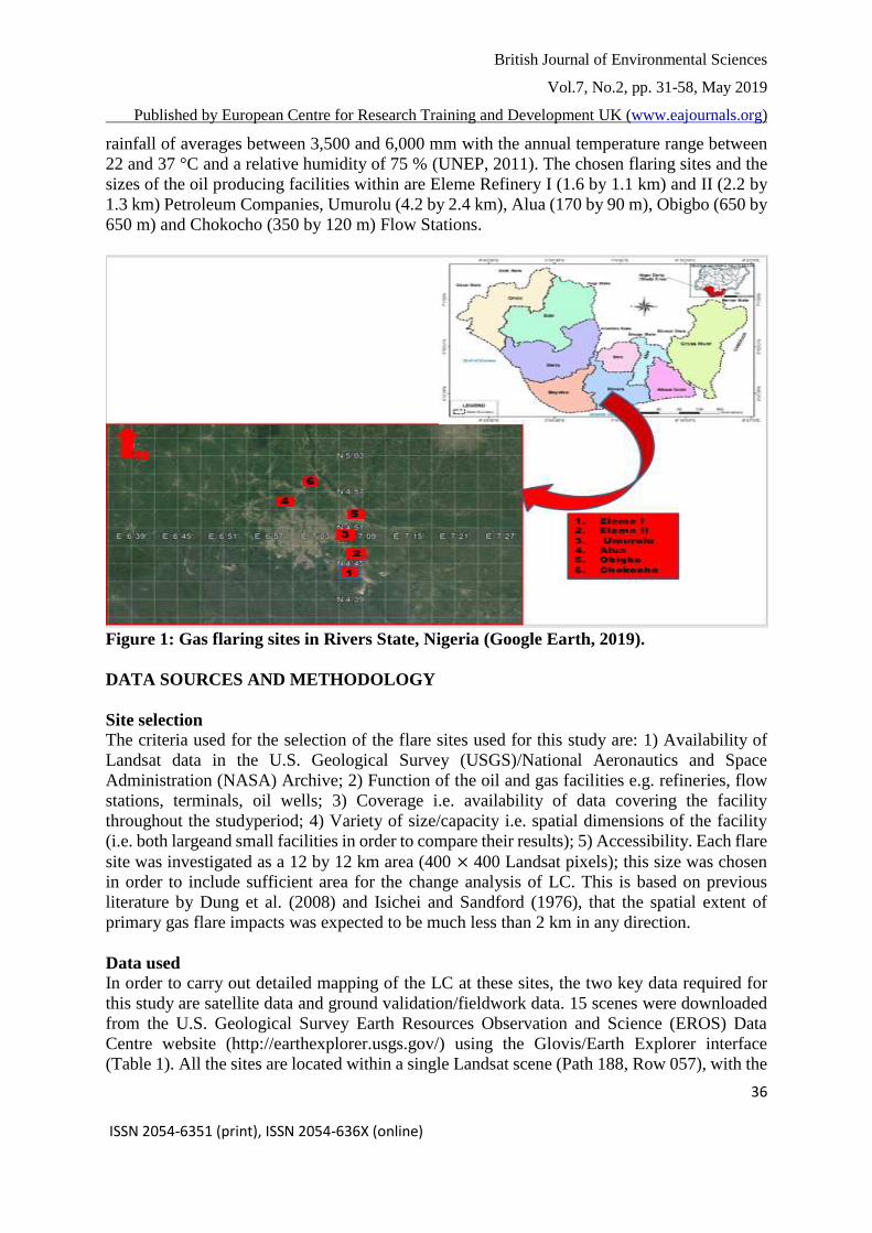
This study focuses on 6 gas flaring sites located in Rivers State of the Niger Delta region,

Nigeria between the Latitude 04° 40' to 05 °55' N and Longitude 06° 50' to 07° 05' E (Bekwe,

2003) (Figure 1). The topography of River State is generally low-lying with heights of not more

than 3 m above sea level and is generally covered by fresh water swamp, mangrove swamp,

lagoonal marshes, tidal channels, beach ridges and sand bars (Dublin-Green et al., 1999). Its

vegetation is an arcuate shaped basin with diverse vegetation which is characterized by 4

distinct ecological zones: coastal ridge barriers, brackish/freshwater swamp forests, mangrove

forests and lowland rain forests, each of which offers diversity of setting for ecological

resources and human activities (Odukoya, 2006; Onosode, 2003). Rivers State has an annual



Vol.7, No.2, pp. 31-58, May 2019



rainfall of averages between 3,500 and 6,000 mm with the annual temperature range between

22 and 37 °C and a relative humidity of 75 % (UNEP, 2011). The chosen flaring sites and the

sizes of the oil producing facilities within are Eleme Refinery I (1.6 by 1.1 km) and II (2.2 by

1.3 km) Petroleum Companies, Umurolu (4.2 by 2.4 km), Alua (170 by 90 m), Obigbo (650 by

650 m) and Chokocho (350 by 120 m) Flow Stations.

Figure 1: Gas flaring sites in Rivers State, Nigeria (Google Earth, 2019).

DATA SOURCES AND METHODOLOGY

Site selection The criteria used for the selection of the flare sites used for this study are: 1) Availability of

Landsat data in the U.S. Geological Survey (USGS)/National Aeronautics and Space

Administration (NASA) Archive; 2) Function of the oil and gas facilities e.g. refineries, flow

stations, terminals, oil wells; 3) Coverage i.e. availability of data covering the facility

throughout the studyperiod; 4) Variety of size/capacity i.e. spatial dimensions of the facility

(i.e. both largeand small facilities in order to compare their results); 5) Accessibility. Each flare

site was investigated as a 12 by 12 km area (400 × 400 Landsat pixels); this size was chosen

in order to include sufficient area for the change analysis of LC. This is based on previous

literature by Dung et al. (2008) and Isichei and Sandford (1976), that the spatial extent of

primary gas flare impacts was expected to be much less than 2 km in any direction.

Data used In order to carry out detailed mapping of the LC at these sites, the two key data required for

this study are satellite data and ground validation/fieldwork data. 15 scenes were downloaded

from the U.S. Geological Survey Earth Resources Observation and Science (EROS) Data

Centre website (http://earthexplorer.usgs.gov/) using the Glovis/Earth Explorer interface

(Table 1). All the sites are located within a single Landsat scene (Path 188, Row 057), with the



Vol.7, No.2, pp. 31-58, May 2019



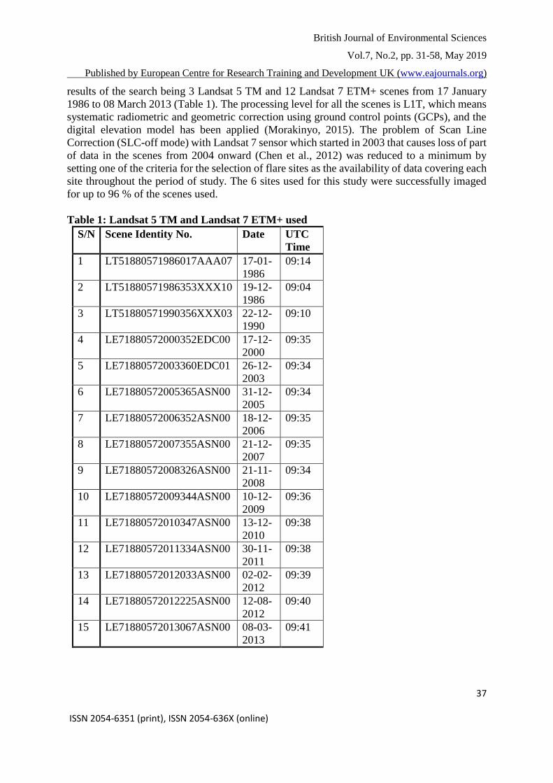
results of the search being 3 Landsat 5 TM and 12 Landsat 7 ETM+ scenes from 17 January

1986 to 08 March 2013 (Table 1). The processing level for all the scenes is L1T, which means

systematic radiometric and geometric correction using ground control points (GCPs), and the

digital elevation model has been applied (Morakinyo, 2015). The problem of Scan Line

Correction (SLC-off mode) with Landsat 7 sensor which started in 2003 that causes loss of part

of data in the scenes from 2004 onward (Chen et al., 2012) was reduced to a minimum by

setting one of the criteria for the selection of flare sites as the availability of data covering each

site throughout the period of study. The 6 sites used for this study were successfully imaged

for up to 96 % of the scenes used.

Table 1: Landsat 5 TM and Landsat 7 ETM+ used

S/N Scene Identity No. Date UTC

Time

1 LT51880571986017AAA07 17-01-

1986

09:14

2 LT51880571986353XXX10 19-12-

1986

09:04

3 LT51880571990356XXX03 22-12-

1990

09:10

4 LE71880572000352EDC00 17-12-

2000

09:35

5 LE71880572003360EDC01 26-12-

2003

09:34

6 LE71880572005365ASN00 31-12-

2005

09:34

7 LE71880572006352ASN00 18-12-

2006

09:35

8 LE71880572007355ASN00 21-12-

2007

09:35

9 LE71880572008326ASN00 21-11-

2008

09:34

10 LE71880572009344ASN00 10-12-

2009

09:36

11 LE71880572010347ASN00 13-12-

2010

09:38

12 LE71880572011334ASN00 30-11-

2011

09:38

13 LE71880572012033ASN00 02-02-

2012

09:39

14 LE71880572012225ASN00 12-08-

2012

09:40

15 LE71880572013067ASN00 08-03-

2013

09:41



Vol.7, No.2, pp. 31-58, May 2019



Methods for data processing

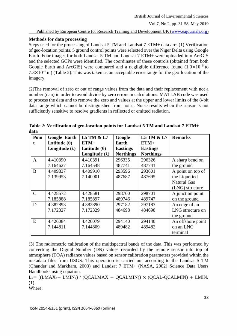
Steps used for the processing of Landsat 5 TM and Landsat 7 ETM+ data are: (1) Verification

of geo-location points. 5 ground control points were selected over the Niger Delta using Google

Earth. Four images for both Landsat 5 TM and Landsat 7 ETM+ were uploaded into ArcGIS

and the selected GCPs were identified. The coordinates of these controls (obtained from both

Google Earth and ArcGIS) were compared and a negligible difference found (1.0×10⁻6 to

7.3×10⁻6 m) (Table 2). This was taken as an acceptable error range for the geo-location of the

imagery.

(2)The removal of zero or out of range values from the data and their replacement with not a

number (nan) in order to avoid divide by zero errors in calculations. MATLAB code was used

to process the data and to remove the zero and values at the upper and lower limits of the 8-bit

data range which cannot be distinguished from noise. Noise results when the sensor is not

sufficiently sensitive to resolve gradients in reflected or emitted radiation.

Table 2: Verification of geo-location points for Landsat 5 TM and Landsat 7 ETM+

data

Poin

t

Google Earth

Latitude (θ)

Longitude (λ)

L5 TM & L7

ETM+

Latitude (θ)

Longitude (λ)

Google

Earth

Eastings

Northings

L5 TM & L7

ETM+

Eastings

Northings

Remarks

A 4.410390

7.164627

4.410391

7.164548

296335

487741

296326

487741

A sharp bend on

the ground

B 4.409837

7.139953

4.409910

7.140001

293596

487687

293601

487695

A point on top of

the Liquefied

Natural Gas

(LNG) structure

C 4.428572

7.185888

4.428581

7.185897

298700

489746

298701

489747

A junction point

on the ground

D 4.382893

7.172327

4.382890

7.172329

297182

484698

297183

484698

An edge of an

LNG structure on

the ground

E 4.426084

7.144811

4.426079

7.144809

294140

489482

294140

489482

An offshore point

on an LNG

terminal

(3) The radiometric calibration of the multispectral bands of the data. This was performed by

converting the Digital Number (DN) values recorded by the remote sensor into top of

atmosphere (TOA) radiance values based on sensor calibration parameters provided within the

metadata files from USGS. This operation is carried out according to the Landsat 5 TM

(Chander and Markham, 2003) and Landsat 7 ETM+ (NASA, 2002) Science Data Users

Handbooks using equation.

Lλ= ((LMAXλ− LMINλ) / (QCALMAX − QCALMIN)) × (QCAL-QCALMIN) + LMINλ

(1)

Where:



Vol.7, No.2, pp. 31-58, May 2019



Lλ= Spectral Radiance at the sensor’s aperture in Wm-²sr-¹µm-¹;

QCAL = the quantized calibrated pixel value in DN (Digital Number);

LMINλ= the spectral radiance that is scaled to QCALMIN in Wm-²sr-¹µm-¹;

LMAXλ= the spectral radiance that is scaled to QCALMAX in Wm-²sr-¹µm-¹;

QCALMIN = the minimum quantized calibrated pixel value (corresponding to LMINλ) in DN

= 1 for LPGS (a processing software version) products;

QCALMAX = the maximum quantized calibrated pixel value (corresponding to LMAXλ) in

DN = 255

(4) Computation of TOA reflectance for multispectral bands 1 to 4, including the application

of simple Sun angle correction using equation 2.

𝜌p = (𝜋 × Lλ × d²) ÷ (ESUNλ × cos 𝜃𝑠) (2)

Where:

𝜌p = Unitless effective at-satellite planetary reflectance;

L is measured per unit solid angle;

𝜋L = Upwelling radiance over a full hemisphere;

d = Earth-Sun distance in astronomical units

ESUNλ = Mean solar exoatmospheric irradiances.

𝜃𝑠 = Solar zenith incident angle in degrees (Chander and Markham, 2003).

(5) Correction for the atmospheric effects for the multispectral bands (1-4) to retrieve the real

surface parameters by removing the atmospheric effects, such as (potentially) thin clouds

(Inamdar et al., 2008), molecular and aerosol scattering, absorption by gases (such as water

vapour, ozone, oxygen) and aerosol, and sometime also the correction for cloud shadows,

upward emission of the radiation from the Earth surface (Qin et al., 2011), environmental

radiance which produces the adjacency effects, variation of illumination geometry including

the Sun’s azimuth and zenith angles, and ground slope (Mather, 2004). Accordingly, the visible

bands of Landsat 5 TM and Landsat 7 ETM+ are more strongly affected by varying

atmospheric conditions than the infrared and mid-infrared bands. Atmospheric correction

consists of two major steps: parameter estimation and surface reflectance retrieval (Liang et

al., 2001). The most difficult component of atmospheric correction is to eliminate the effect of

aerosols. The fact that most aerosols are often distributed heterogeneously makes this task more

difficult (Liang et al., 2001).

The methods reported in the literature for the quantitative atmospheric correction of Landsat 5

TM and Landsat 7 ETM+ imagery visible and NIR bands can be roughly classified into the

following groups: Invariant-object, histogram matching, dark object subtraction (DOS), and

contrast reduction (Liang et al., 2001). DOS method have a long history (Kaufman et al., 2000;

Liang et al., 1997; Teillet and Fedosejevs, 1995) and are probably the most popular

atmospheric correction method (Liang et al., 2001) reported in the literature. The basic

assumption is that within the image some pixels are in complete shadow and their radiances

received at the satellite are due to the atmospheric scattering (path radiance). This assumption

is combined with the fact that very few targets on the Earth’s surface are absolute black, so an

assumed 1 % minimum reflectance is better than 0 % (Chavez, 1996). Both MODIS and

medium resolution imaging spectroradiometer (MERIS) atmospheric correction algorithms



Vol.7, No.2, pp. 31-58, May 2019



(Santer et al., 1999) are based on this principle. However, this method assumes that this error

is the same over the whole image (Liang et al., 2001).

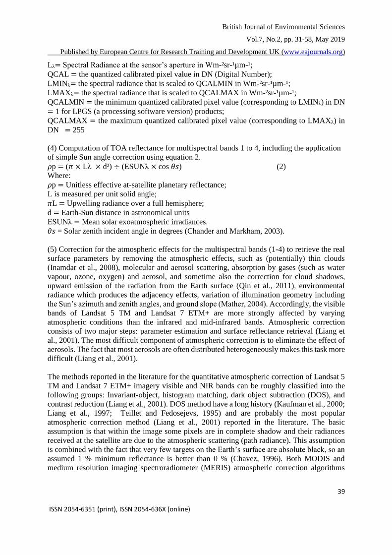
For this study, DOS method was used and its principle applied to this study means that pixels

corresponding to the darkest location (Atlantic Ocean) were selected for each band 1 to 4 (Table

3). The number of pixels obtained varies depending on the size of the darkest spot. The

reflectance for these dark pixels was computed for each band and the minimum value obtained

for each band was used as an estimate of the atmospheric reflectance for the respective band.

These small errors were subtracted from the computed reflectance for each pixel of the whole

image to reduce the atmospheric effects.

Table 3: Latitude and Longitude of some dark pixels over Atlantic Ocean

Image ID Band 1

(Lat. /Long.)

Band 2

(Lat. /Long.)

Band 3

(Lat. /Long.)

Band 4

(Lat. /Long.)

LT51880571986

017AAA04

4.336699

7.250121

4.332076

7.257068

4.336710

7.254742

4.327437

7.257078

LT51880571987

004XXX04

4.169107

7.074345

3.798029

7.699768

3.792277

7.694059

3.788445

7.690256

LT51880571986

353XXX10

4.281913

7.366087

4.183774

7.659434

4.138324

7.352093

4.076853

7.143137

LE71880571999

333AGS00

3.665176

6.592174

3.665176

6.592174

3.723996

6.567263

3.664760

6.592157

LE71880572000

352EDC00

4.281250

8.164940

4.282325

8.163866

4.281548

8.164345

4282569

8.163037

LE71880572003

008SGS00

3.591636

7.948805

3.594024

7.948802

3.598809

7.948797

3.596421

7.948800

Land cover mapping and classification

The accuracy of LULC classification are of great significance to global change, environmental

monitoring etc. (Yuechen et al., 2012). However, there is no uniform standard for LULC

classification at present, which brings a lot of inconvenience to the collection and analysis of

LC data (Yue et al., 2018). Several researchers have worked on LULC analysis using different

methods to achieve their results. For example, Aixia et al. (2006) applied fuzzy K-means non-

supervised classifier to get 4 classes of the LC. Yuechen et al. (2012) adopted supervised digital

classification using maximum likelihood classifier for identifying 8 classes of LULC.

Maaharjan (2018) adopted interactive supervised image classification system to obtain 4

classes. Kayet et al. (2018) and Fonteh et al. (2016) employed Support Vector Machine (SVM)

method for separation of 10 LULC classes (water, settlement, bare ground, dark mangroves,

green mangroves, swampy vegetation, rubber, coastal forest and other vegetation and palms)

(Fonteh et al., 2016). SVM is more advantageous in object-based classification and image

analysis (Tan and Zhang, 2008; Tzotsos and Argialas, 2008).



Vol.7, No.2, pp. 31-58, May 2019



A stochastic model was combined with visual interpretation to estimate and evaluate the change

detection for 3 classes (Yuechen et al. (2012) of LC (Built up, non- urban and water bodies)

(Pareta, 2014). In addition, Chen and Li (2004) applied Soil and Water Assessment Tool

(SWAT) model to simulate different LC. Furthermore, Niehoff et al. (2002) used LU change

modelling kit (LUCK) with a modified version of the physically-based hydrological model

WaSiM-ETH for flood prediction. Tomar et al. (2017) used image processing method in

ERDAS imagine and ArcGIS 10.3 for detection of 5 classes of LULC changes. Boori and

Voženílek (2014) adopted object-oriented classification method for 3 classes of LC. In

addition, 5 LULC classes namely built up, agriculture land, open space, vegetation and water

body were identified by Shravya and Sridhar (2017).

For this study, the first unsupervised cluster analysis (Alvarez, 2009; Hestir et al., 2008) of the

atmospherically corrected reflectance (bands 1-4) using the K-means function (Şatır and

Berberoğlu., 2012; Hestir et al., 2008) of the MATLAB tool was carried out. The results

obtained give 3 classes of LC type with cloud classified as the 4th class. The 4 classes identified

are any of these 3: vegetation, water, soil and built up area, and cloud as the 4th class. The next

stage was the elimination of the class for the cloud by masking using MATLAB code. The

second cluster analysis was performed with the cloud-masked reflectance (bands 1-4) to give

4 (Maaharjan, 2018; Boori et al., 2015) (vegetation, soil, built up area and water) LC types for

all sites. Landsat Short Wave Infra-Red (SWIR) bands 5 and 7 were also employed for the

classification of LC types but they could not give useful information as bands 1-4 hence, they

were dropped for further analysis. LC types at these flaring sites change from scene to scene

and from site to site. Furthermore, through visit to the Niger Delta, fieldwork observation and

measurements for ground validation of Landsat 5 TM and Landsat 7 ETM+ took place at Eleme

Refinery I and II in August and September, 2012, during a period of six weeks. It was

confirmed that LC types at these flaring sites are vegetation, some buildings, open land i.e. bare

soil and water bodies. Also, LC types for other 4 flaring sites are similar to that of Eleme

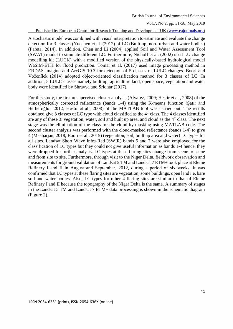
Refinery I and II because the topography of the Niger Delta is the same. A summary of stages

in the Landsat 5 TM and Landsat 7 ETM+ data processing is shown in the schematic diagram

(Figure 2).



Vol.7, No.2, pp. 31-58, May 2019



Figure 2: Schematic diagram for the processing of Landsat 5 TM and Landsat 7 ETM+

for mapping and classification of land cover types at flaring sites in the Niger Delta.

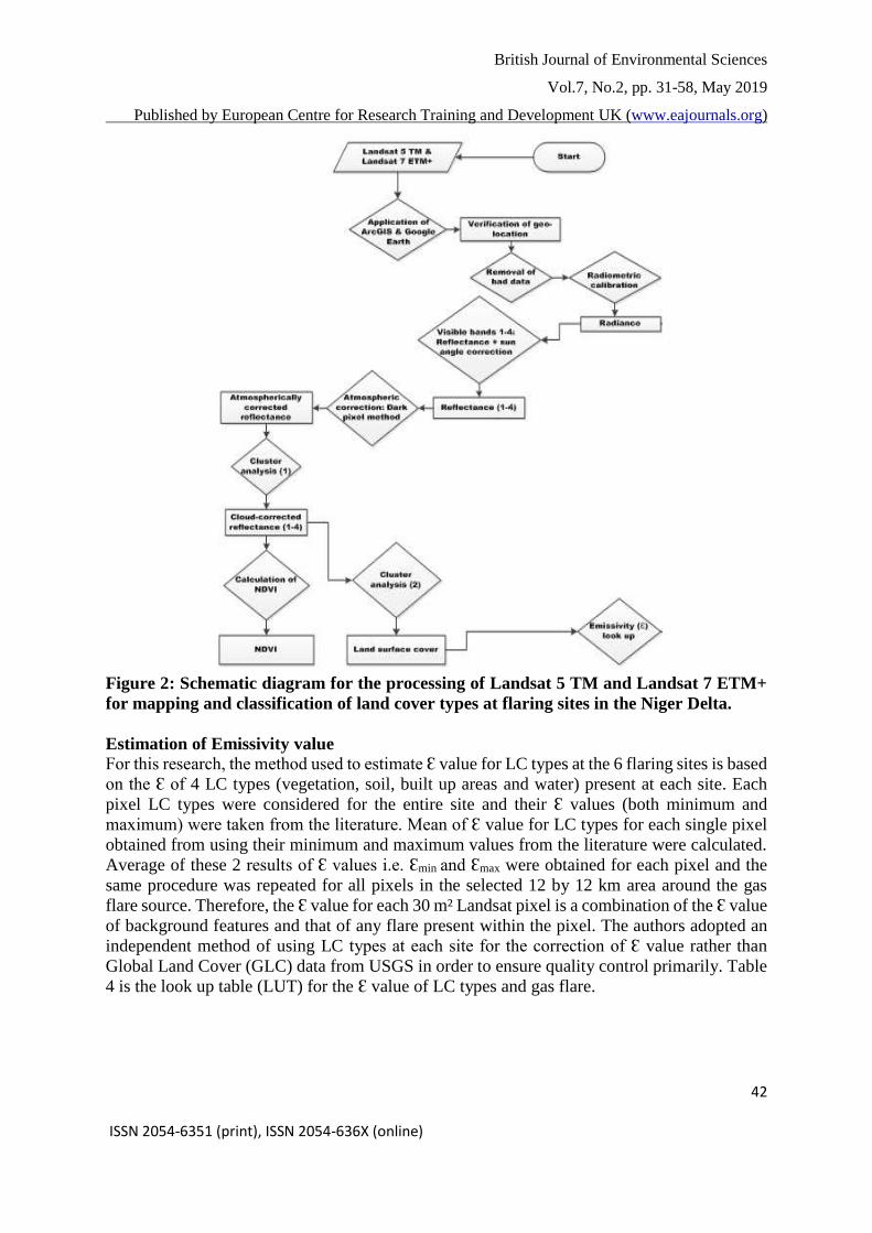
Estimation of Emissivity value

For this research, the method used to estimate Ɛ value for LC types at the 6 flaring sites is based

on the Ɛ of 4 LC types (vegetation, soil, built up areas and water) present at each site. Each

pixel LC types were considered for the entire site and their Ɛ values (both minimum and

maximum) were taken from the literature. Mean of Ɛ value for LC types for each single pixel

obtained from using their minimum and maximum values from the literature were calculated.

Average of these 2 results of Ɛ values i.e. Ɛmin and Ɛmax were obtained for each pixel and the

same procedure was repeated for all pixels in the selected 12 by 12 km area around the gas

flare source. Therefore, the Ɛ value for each 30 m² Landsat pixel is a combination of the Ɛ value

of background features and that of any flare present within the pixel. The authors adopted an

independent method of using LC types at each site for the correction of Ɛ value rather than

Global Land Cover (GLC) data from USGS in order to ensure quality control primarily. Table

4 is the look up table (LUT) for the Ɛ value of LC types and gas flare.



Vol.7, No.2, pp. 31-58, May 2019



Table 4: Surface emissivity for land cover types and gas flares

Land cover type Emissivity value

(minimum)

Emissivity value

(maximum)

Reference

Vegetated areas:

Short grass 0.979 0.983 Labed and Stoll, 1991

Bushes (≈ 100 cm) 0.994 Labed and Stoll, 1991

Densely vegetated

areas

0.960 0.980 Jin and Liang, 2006

Soils:

Bare soil 0.960 Humes et al., 1994

Bare soil (desert) 0.900 Jin and Liang, 2006

Bare soil (sandy) 0.930 Hipps, 1989

Bare soil (loamy sand) 0.914 van de Griend et al.,

1991

Water body:

Water body 0.950 0.980 Masuda et al., 1988

Water body 0.990 Stathopoulou and

Cartalis, 2007

Built up areas:

Medium built 0.964 Stathopoulou and

Cartalis, 2007

Densely urban 0.946 Stathopoulou and

Cartalis, 2007

Flare:

0.13 0.40 Shore, 1996

0.15 0.30 PTT, 2008

0.18 0.25 Sáez, 2010

RESULTS/ FINDINGS

Land cover types

In order to achieve the aim of this study, the following analysis steps were used for the

classification and ascertaining of LC types at these flaring sites: an overview of spatial

variability in land use that was achieved using simple visual examination of Worldview-1 and

2 and IKONOS pseduo-true colour images accessed through Google Earth and Digital Global

(http://browse.digitalglobe.com/imagefinder/public.do). The LC classification results were

used to summarise the LC types around each site. Then, the Landsat reflective bands were

examined to identify any unusual ground features associated. Finally, the pseudo-true colour

images from the combination of bands 3, 2 and 1 as red, green and blue (RGB) were included

as a comparison to the higher spatial resolution WorldView and IKONOS browse images in

identifying features at each site (the green features in the Landsat RGB image should

correspond to green features in Google Earth) (Figures 3-8). Other Landsat bands combination

such as Red, Green and Near Infrared bands; Green, Blue and Near Infrared; Red, Green and

Short-Wave Infrared (band 5) and Red, Green and Short-Wave Infrared (band 7) were also


http://browse.digitalglobe.com/imagefinder/public.do


Vol.7, No.2, pp. 31-58, May 2019



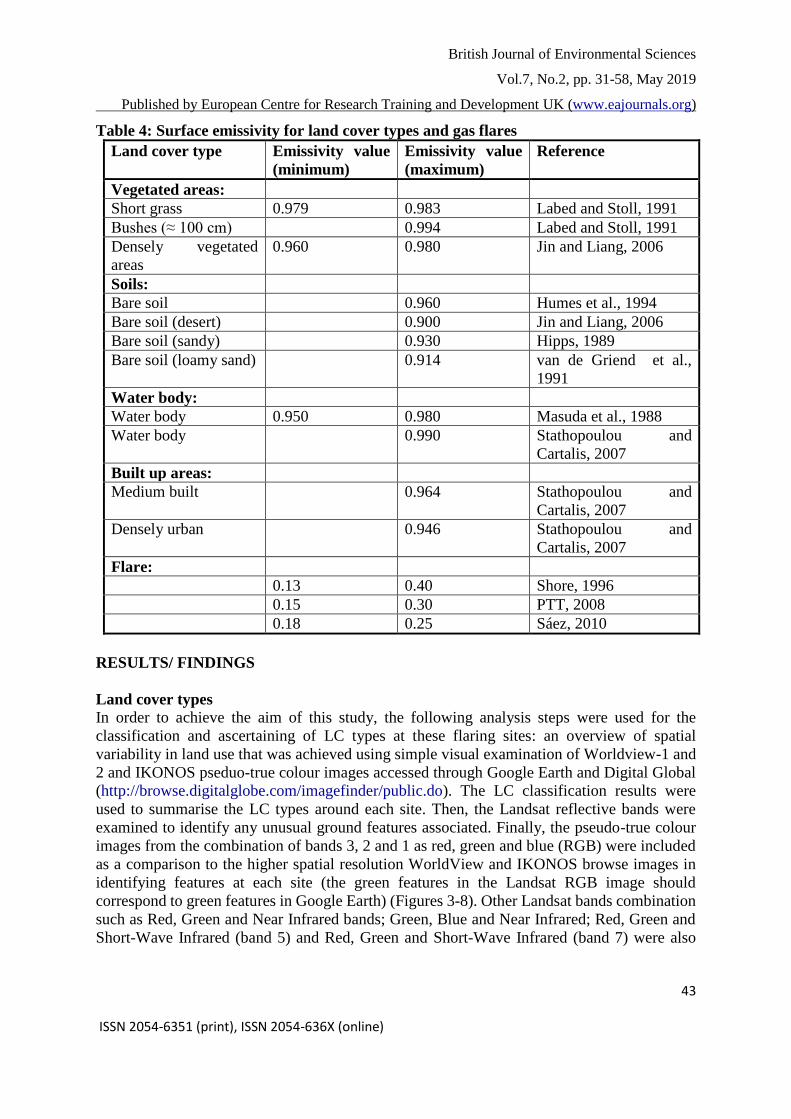
processed to obtain their pseudo-true colour images. The combination of RGB bands gives the

best result and so it was used for the qualitative analysis of this study.

Figure 3: Eleme Refinery I Petroleum Company site: A) in 2000; B) in 2019; C) Bands 1-

4, 6, RGB (8/3/2013) and land cover types (17/1/1986 & 8/3/2013), (X and Y axes: pixel

numbers; scale bar: digital number, DN)

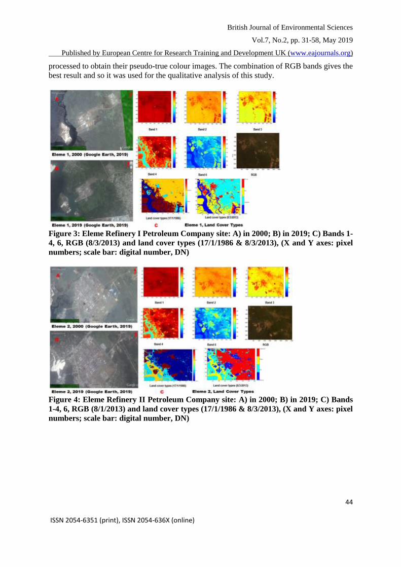
Figure 4: Eleme Refinery II Petroleum Company site: A) in 2000; B) in 2019; C) Bands

1-4, 6, RGB (8/1/2013) and land cover types (17/1/1986 & 8/3/2013), (X and Y axes: pixel

numbers; scale bar: digital number, DN)



Vol.7, No.2, pp. 31-58, May 2019



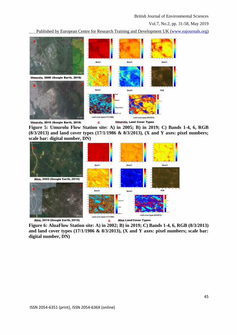
Figure 5: Umurolu Flow Station site: A) in 2005; B) in 2019; C) Bands 1-4, 6, RGB

(8/3/2013) and land cover types (17/1/1986 & 8/3/2013), (X and Y axes: pixel numbers;

scale bar: digital number, DN)

Figure 6: AluaFlow Station site: A) in 2002; B) in 2019; C) Bands 1-4, 6, RGB (8/3/2013)

and land cover types (17/1/1986 & 8/3/2013), (X and Y axes: pixel numbers; scale bar:

digital number, DN)



Vol.7, No.2, pp. 31-58, May 2019



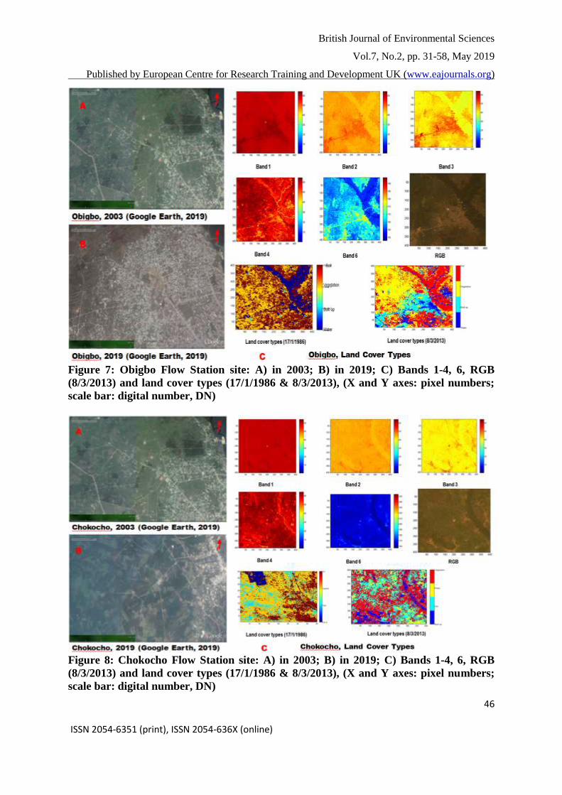
Figure 7: Obigbo Flow Station site: A) in 2003; B) in 2019; C) Bands 1-4, 6, RGB



Figure 8: Chokocho Flow Station site: A) in 2003; B) in 2019; C) Bands 1-4, 6, RGB





Vol.7, No.2, pp. 31-58, May 2019



Figures 3 A & B shows that there is infrastructural development and great expansion of built

up such as buildings and road networks toward the North-West, East and spreading toward

East-South and East-North of the Eleme Refinery I site from 1986 to 2019; construction of

roads at the North-East side and across the river has taken place in Figures 3 C and LC types

of 8/3/2013. These leads to reduction on bear soil and vegetation cover. Figures 4 A, B & C

shows the state of Eleme Refinery II site in 1986, 2000, 2013 and 2019 with developmental

growth in number of built up around the refinery that spread toward West, South-West in 2019

compared to 2000; its LC map (8/3/2013) shows the increase in built up area such as buildings,

roads that were not available in 1986. These have caused reduction in bare soil and vegetation

cover within the site. For Umurolu site (Figures 5 A, B & C), there is an increase in built up

area around the flow station and massive infrastructural development due to human settlements

towards the West, North-West and South-West of the site on LC map (8/3/2013) and the

Google Earth image of 2019 that were not present on LC map (17/1/1986) and the Google

Earth image of 2005. This size of soil and vegetation cover has been greatly reduced.

Figures 6 A, B & C shows that in 2013 and 2019 there are more built up areas at the West and

South-East areas of Alua site as compared to 1986; in LC map (17/1/1986), a portion of the

site towards North-East and East-South with soil and vegetation have been replaced with water

in 8/3/2013. In addition, some portions of the site from the centre toward North and spread

towards North-East that were covered with water in 17/1/1986 map have been replaced with

vegetation in 8/1/2013 map. Roads are presented at the North-East, South-West and almost

diagonally from the South-East to the North-East of the site in 8/3/2013 map. Figures 7 A, B

& C show the explosive urban growth of built up e.g. several houses and route networks at

Obigbo site in 2013 towards 2019 as compared to 1986.

There is massive settlement at the centre of the site, spreading toward South-East, South, South-

West in 8/3/2013 map but not available in 17/1/1986 map. There is also, built up development

at the North, towards North-East after the river in 8/3/2013 map that is not shown in 17/1/1986

map. In 17/1/1986 map, the width of the flowing river is wider while it has been narrowed in

8/3/2013 map. There are significant reduction changes in soil and vegetation cover in 2013

towards 2019 compared to 1986. For Chokocho, Figures 8 A, B & C shows a large building at

the North-West of the site in 1986 which is no more in 2013. Growth in the settlement at the

East, South and South-West of the site is shown in 8/3/2013 map. There is also a road

development linked North-East to the East in 8/3/2013 map while it was not available in

17/1/1986 map. Generally, the influence of the activities of crude oil production and refining,

infrastructural development and other human activities including farming, logging etc. have

change LC at all sites, affects LC negatively and causes degradation of the ecosystem.



Vol.7, No.2, pp. 31-58, May 2019



Estimation of Emissivity value

The Ɛ results (Table 5) from LC types at each flaring site are obtained from 1 season (dry) out

of 2 seasons (rain and dry) available in Nigeria. The emissivity value recorded for vegetation,

built up, water and soil at each site vary from 1986 to 2013. Since Ɛ is strongly dependent on

LULC types (Mallick et al., 2012), this study applied Ɛ values to evaluate the % of LC loss for

the 4 LC types available at the sites investigated. Generally, the Ɛ values obtained for 4 LC

types for all sites in 1986 is higher than those obtained in 2013. In 1986, vegetation cover has

the highest Ɛ values throughout the entire 6 sites, followed by water. In 2013, the Ɛ values

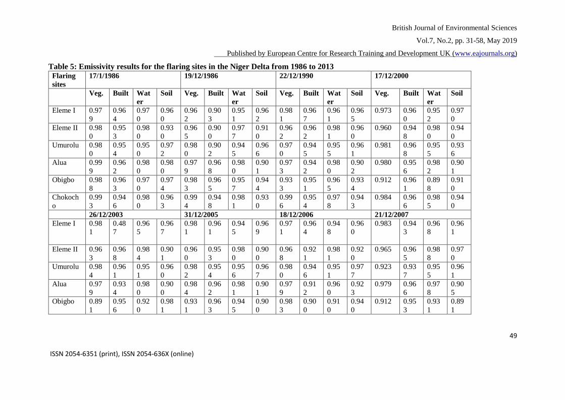
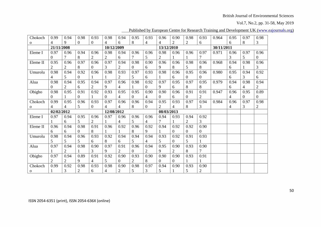
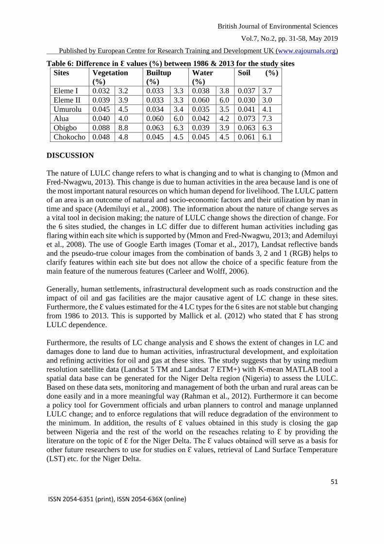
recorded for the same 4 LC within the sites have been greatly reduced. Table 6 shows the

difference in Ɛ values (%) obtained in 1986 and that of 2013 for 6 sites investigated. The % of

vegetation cover loss for all sites shows Obigbo site is with the highest (8.8 %) and Eleme I

site is with the lowest (3.2 %). The % of increase in built up LC also shows Obigbo site having

the highest (6.3 %) while both Eleme I and II gives the lowest (3.3 %). Eleme II has the highest

% of water LC loss (6.0 %) while Umurolu site shows the lowest (3.5 %). For soil LC, Alua

site has the highest % of loss (7.3 %) while Eleme II recorded the lowest (3.7 %). In summary,

the % of LC loss recorded could be attributed to the impact of crude oil production and refining

activities, infrastructural development and other human activities such as farming, logging etc.



Vol.7, No.2, pp. 31-58, May 2019



Table 5: Emissivity results for the flaring sites in the Niger Delta from 1986 to 2013

Flaring

sites

17/1/1986 19/12/1986 22/12/1990 17/12/2000

Veg. Built Wat

er

Soil Veg. Built Wat

er

Soil Veg. Built Wat

er

Soil Veg. Built Wat

er

Soil

Eleme I 0.97

9

0.96

4

0.97

0

0.96

0

0.96

2

0.90

3

0.95

1

0.96

2

0.98

1

0.96

7

0.96

1

0.96

5

0.973 0.96

0

0.95

2

0.97

0

Eleme II 0.98

0

0.95

3

0.98

0

0.93

0

0.96

5

0.90

0

0.97

7

0.91

0

0.96

2

0.96

2

0.98

1

0.96

0

0.960 0.94

8

0.98

0

0.94

0

Umurolu 0.98

0

0.95

4

0.95

0

0.97

2

0.98

0

0.90

2

0.94

5

0.96

6

0.97

0

0.94

5

0.95

5

0.96

1

0.981 0.96

8

0.95

5

0.93

6

Alua 0.99

9

0.96

2

0.98

0

0.98

0

0.97

9

0.96

8

0.98

0

0.90

1

0.97

3

0.94

2

0.98

0

0.90

2

0.980 0.95

6

0.98

2

0.90

1

Obigbo 0.98

8

0.96

3

0.97

0

0.97

4

0.98

3

0.96

5

0.95

7

0.94

4

0.93

3

0.95

1

0.96

5

0.93

4

0.912 0.96

1

0.89

8

0.91

0

Chokoch

o

0.99

3

0.94

6

0.98

0

0.96

3

0.99

4

0.94

8

0.98

1

0.93

0

0.99

6

0.95

4

0.97

8

0.94

3

0.984 0.96

6

0.98

5

0.94

0

26/12/2003 31/12/2005 18/12/2006 21/12/2007

Eleme I 0.98

1

0.48

7

0.96

5

0.96

7

0.98

1

0.96

1

0.94

5

0.96

9

0.97

1

0.96

4

0.94

8

0.96

0

0.983

0.94

3

0.96

8

0.96

1

Eleme II 0.96

3

0.96

8

0.98

4

0.90

1

0.96

0

0.95

3

0.98

0

0.90

0

0.96

8

0.92

1

0.98

1

0.92

0

0.965 0.96

5

0.98

8

0.97

0

Umurolu 0.98

4

0.96

1

0.95

1

0.96

0

0.98

2

0.95

4

0.95

6

0.96

7

0.98

0

0.94

6

0.95

1

0.97

7

0.923 0.93

7

0.95

5

0.96

1

Alua 0.97

9

0.93

4

0.98

0

0.90

0

0.98

4

0.96

2

0.98

1

0.90

1

0.97

9

0.91

2

0.96

0

0.92

3

0.979 0.96

6

0.97

8

0.90

5

Obigbo 0.89

1

0.95

6

0.92

0

0.98

1

0.93

1

0.96

3

0.94

5

0.90

0

0.98

3

0.90

0

0.91

0

0.94

0

0.912 0.95

3

0.93

1

0.89

1



Vol.7, No.2, pp. 31-58, May 2019



Chokoch

o

0.99

4

0.94

9

0.98

0

0.93

0

0.98

4

0.94

6

0.95

8

0.93

4

0.96

4

0.90

2

0.98

2

0.93

6

0.964 0.95

6

0.97

8

0.98

3

21/11/2008 10/12/2009 13/12/2010 30/11/2011

Eleme I 0.97

0

0.96

7

0.94

8

0.96

2

0.98

2

0.94

6

0.96

7

0.96

5

0.98

2

0.96

1

0.96

1

0.97

7

0.971 0.96

3

0.97

5

0.96

0

Eleme II 0.95

2

0.96

2

0.97

8

0.96

0

0.97

3

0.94

2

0.98

0

0.90

6

0.96

9

0.96

8

0.98

5

0.96

8

0.968 0.94

6

0.98

1

0.96

3

Umurolu 0.98

4

0.94

5

0.92

0

0.96

1

0.98

1

0.93

2

0.97

5

0.93

6

0.98

1

0.96

6

0.95

0

0.96

0

0.980 0.95

6

0.94

3

0.92

6

Alua 0.98

0

0.94

2

0.95

6

0.94

2

0.97

9

0.96

4

0.98

1

0.92

0

0.97

9

0.95

6

0.97

8

0.95

8

0.979 0.94

6

0.98

4

0.94

2

Obigbo 0.98

0

0.95

1

0.91

0

0.92

1

0.93

0

0.95

4

0.95

0

0.90

4

0.90

0

0.96

6

0.91

0

0.91

2

0.947 0.96

4

0.95

0

0.89

0

Chokoch

o

0.99

4

0.95

4

0.96

5

0.93

0

0.97

4

0.96

4

0.96

8

0.94

0

0.95

2

0.93

4

0.97

8

0.94

3

0.984 0.96

4

0.97

3

0.98

2

02/02/2012 12/08/2012 08/03/2013

Eleme I 0.97

1

0.94

6

0.95

5

0.96

2

0.97

1

0.96

4

0.96

5

0.96

4

0.94

7

0.93

1

0.94

2

0.92

3

Eleme II 0.96

6

0.94

6

0.98

0

0.91

8

0.96

1

0.92

1

0.96

8

0.92

9

0.94

1

0.92

0

0.92

0

0.90

0

Umurolu 0.98

5

0.94

5

0.96

5

0.93

6

0.92

8

0.94

6

0.94

5

0.94

4

0.93

5

0.92

0

0.91

5

0.93

1

Alua 0.97

1

0.94

2

0.98

1

0.90

3

0.97

9

0.91

2

0.96

0

0.94

2

0.95

9

0.90

2

0.93

8

0.90

7

Obigbo 0.97

2

0.94

2

0.89

9

0.91

4

0.92

5

0.90

0

0.93

2

0.90

8

0.90

0

0.90

0

0.93

1

0.91

1

Chokoch

o

0.99

1

0.92

3

0.98

2

0.93

6

0.98

4

0.90

2

0.98

5

0.97

3

0.94

5

0.90

1

0.93

5

0.90

2



Vol.7, No.2, pp. 31-58, May 2019



Table 6: Difference in Ɛ values (%) between 1986 & 2013 for the study sites

Sites Vegetation

(%)

Builtup

(%)

Water

(%)

Soil (%)

Eleme I 0.032 3.2 0.033 3.3 0.038 3.8 0.037 3.7

Eleme II 0.039 3.9 0.033 3.3 0.060 6.0 0.030 3.0

Umurolu 0.045 4.5 0.034 3.4 0.035 3.5 0.041 4.1

Alua 0.040 4.0 0.060 6.0 0.042 4.2 0.073 7.3

Obigbo 0.088 8.8 0.063 6.3 0.039 3.9 0.063 6.3

Chokocho 0.048 4.8 0.045 4.5 0.045 4.5 0.061 6.1

DISCUSSION

The nature of LULC change refers to what is changing and to what is changing to (Mmon and

Fred-Nwagwu, 2013). This change is due to human activities in the area because land is one of

the most important natural resources on which human depend for livelihood. The LULC pattern

of an area is an outcome of natural and socio-economic factors and their utilization by man in

time and space (Ademiluyi et al., 2008). The information about the nature of change serves as

a vital tool in decision making; the nature of LULC change shows the direction of change. For

the 6 sites studied, the changes in LC differ due to different human activities including gas

flaring within each site which is supported by (Mmon and Fred-Nwagwu, 2013; and Ademiluyi

et al., 2008). The use of Google Earth images (Tomar et al., 2017), Landsat reflective bands

and the pseudo-true colour images from the combination of bands 3, 2 and 1 (RGB) helps to

clarify features within each site but does not allow the choice of a specific feature from the

main feature of the numerous features (Carleer and Wolff, 2006).

Generally, human settlements, infrastructural development such as roads construction and the

impact of oil and gas facilities are the major causative agent of LC change in these sites.

Furthermore, the Ɛ values estimated for the 4 LC types for the 6 sites are not stable but changing

from 1986 to 2013. This is supported by Mallick et al. (2012) who stated that Ɛ has strong

LULC dependence.

Furthermore, the results of LC change analysis and Ɛ shows the extent of changes in LC and

damages done to land due to human activities, infrastructural development, and exploitation

and refining activities for oil and gas at these sites. The study suggests that by using medium

resolution satellite data (Landsat 5 TM and Landsat 7 ETM+) with K-mean MATLAB tool a

spatial data base can be generated for the Niger Delta region (Nigeria) to assess the LULC.

Based on these data sets, monitoring and management of both the urban and rural areas can be

done easily and in a more meaningful way (Rahman et al., 2012). Furthermore it can become

a policy tool for Government officials and urban planners to control and manage unplanned

LULC change; and to enforce regulations that will reduce degradation of the environment to

the minimum. In addition, the results of Ɛ values obtained in this study is closing the gap

between Nigeria and the rest of the world on the reseaches relating to Ɛ by providing the

literature on the topic of Ɛ for the Niger Delta. The Ɛ values obtained will serve as a basis for

other future researchers to use for studies on Ɛ values, retrieval of Land Surface Temperature

(LST) etc. for the Niger Delta.



Vol.7, No.2, pp. 31-58, May 2019



CONCLUSION

This study illustrates the use of RS and K-mean of MATLAB tool as important technologies

for extracting LULC which can be very challenging with the use of conventional mapping

techniques. Assessment of environment is made possible by these technologies in less time, at

low cost and with better accuracy. The results of LC classification obtained shows that the

adopted K-means method can distinguish up to 4 LC types very well in the Niger Delta.

Changing in LC types for all the 6 sites is caused by human activities including farming,

logging, infrastructural developments, and the effects of oil and gas production and refining

activities. This also led to variation in the Ɛ values recorded throughout the period. The LC

changes and Ɛ values recorded in this research will serve as a basis to understand the patterns

and possible consequences of LC changes and Ɛ values in the Niger Delta. In addition, this

study will help to develop new comparative research on the pattern and processes of LC change

in the Niger Delta region and Northern Nigeria; and also to use data from the 2 seasons (dry

and rain) available in Nigeria. Therefore, there is a need for proper land use planning and

enforcement of development control to forestall the negative socio-economic impacts of LULC

changes. Nigerian Government should provide incentives that move individuals from

conflicting relations with their natural system, toward more sustainable landscape transitions;

and there should be the regulatory presence of Nigerian Government (e.g. a ban on logging).

Finally, the future research should pay more attention to the LULC driving factors of social

economy and the natural environment; economic development and technological advancement;

and the exploration of the environmental change effects caused by LULC.

REFERENCE

Ademiluyi, I. A., Okude, A. S and Akanni, C. O. (2008): “An appraisal of land use and land

cover mapping in Nigeria”. African Journal of Agricultural Research 3 (9): 581-586.

Agoha, S. C. (2009): “Analysis of rural-urban land use change in Umuahia, South Eastern

Nigeria”. Unpublished M.Sc. Dissertation submitted to Department of Geography and

Environmental Management University of Abuja.

Aixia, L., Jing, W. and Chunyan, L. V. (2006). “Land cover classification based on MODIS

data in area to the North-West of Beijing”. Progress in Geography 02.

Alvarez, J. (2009). “Land cover verification along Freeway Corridors, Natomas Basin Area,

California, USA”. [Online]. Available:

http://www.academic.emporia.edu/aberjame/student/alvarez4/natchange.htm l

[Accessed 26th September 2016].

Antonarakis, A. S., Richards, K. S and Brasington, J. (2008). “Object-based land cover

classification using airborne LiDAR”. Remote Sensing of Environment 112(6): 2988-

2998.

Awoniran, D. R., Adewole, D., Adegboyega, S. S and Anifowose, Y. (2013). “Assessment of

environmental responses to land use/land cover dynamics in the lower Ogun River

Basin, South-Western Nigeria”. International Journal of Sustainable Land Use and

Urban Planning. ISSN 1927-8845 1(2): 16-31.

Becker, F and Li, Z. L. (1995). “Surface temperature and emissivity at various scales:

definition, measurement and related problems”. Remote Sensing Reviews 12: 225-253.


http://en.cnki.com.cn/Journal_en/A-A008-DLKJ-2006-02.htm


Vol.7, No.2, pp. 31-58, May 2019



Bekwe, W. F. (2003). “Urban flood hazards mapping; A GIS approach: A case study of Port

Harcourt”. Unpublished M.Sc. Dissertation, University of Ibadan, Ibadan.

Bernard, A. C and Wilkinson, G. G. (1997). “Training strategies for neural network soft

classification of remotely-sensed imagery”. International Journal of Remote Sensing

8(8): 1851-1856.

Boori, M. S and Voženílek, V. (2014). “Remote sensing and land use/land cover trajectories.

Journal of Geophysical Remote Sensing 3: 123. doi:10.4172/2169-0049.1000123.

Boori, M. S., Vozenílek, V., Balzter, H and Choudhary, K. (2015). “Land surface temperature

with land cover classes in ASTER and Landsat Data”. Journal of Geophysics and

Remote Sensing 4(1), http://dx.doi.org/10.4172/2169- 0049.1000138.

Braimoh, A. K and Vlek, P. L. G. (2004). “Land cover change analyses in the Volta Basin of

Ghana”. Earth Interact. 8:1-17.

Carleer, A. P and Wolff, E. (2006). “Urban land cover multi-level region-based classification

of VHR data by selecting relevant features”. International Journal of Remote Sensing

27(6): 1035-1051.

Caselles, V and Sobrino, J. A. (1989). “Determination of frosts in orange groves from NOAA-

9 AVHRR data”. Remote Sensing of Environment 29: 135-146.

Chander, G and Markham, K. (2003). “Revised Landsat-5 TM radiometric calibration

procedures and post calibration dynamic ranges”. IEEE Transactions on Geoscience

and Remote Sensing 41(11): 2674-2677.

Chavez, P. S. (1996). “Image-based Atmospheric Corrections-Revisited and Improved”.

Photogrammetry Engineering and Remote Sensing 62(9): 1025-1036

Chen, J. F, Li, X. B. (2004). “Simulations of hydrological response to land cover changes”.

Chinese Journal of Applied Ecology. 15: 833-836.

Chen, F., Zhao, X and Ye, H. (2012). “Making use of the Landsat 7 SLC-off ETM+ image

through different recovering approaches”. Postgraduate Conference on Infrastructure

and Environment (3rd IPCIE), (2): 557-563. [Online]. Available:

http://dx.doi.org/10.5772/48535 [Accessed 26th September 2014].

Desanker, P. V., Frost, P. G. H., Justice, C. O and Scholes, R. J. (1997). “The Miombo

Network: Frameworks for a terrestrial transect study of land use and land cover change

in the Miombo ecosystems of Central Africa”. IGBP Report 41.

Dublin-Green, C. O., Awosika, L. F and Folorunsho, R. (1999). “Climate variability research

activities in Nigeria”. Nigerian Insitute for Oceanography and Marine Research,

Victoria Island, Lagos, Nigeria.

Dung, E. J., Bombom, L. S and Agusomu, T. D. (2008). “The effects of gas flaring on crops in

the Niger Delta, Nigeria”. GeoJournal 73: 297-305.

Ejaro, S. P. (2008): “Analyses of Land use and land cover change in the Federal Capital

Territory (FCT), Abuja using Multi-Temporal Satellite Data”. Unpublished Ph.D

Thesis, Department of Geography and Environmental Management, University of

Abuja, Nigeria.

Fasona, M. J and Omojola, A. S. (2005). “Climate change, human security and communal

clashes in Nigeria”. Paper presented at an International Workshop on Human Security

and Climate Change, Asker, Norway, 21-23.

Fonteh, M. L., Theophile, F., Cornelius, M. L., Main, R., Ramoelo, A and Cho, M. A. (2016).

“Assessing the utility of Sentinel-1 C Band Synthetic Aperture Radar Imagery for land


http://dx.doi.org/10.4172/2169-%200049.1000138

http://dx.doi.org/10.5772/48535


Vol.7, No.2, pp. 31-58, May 2019



use land cover classification in a tropical coastal system When Compared with Landsat

8. Journal of Geographic Information System 8: 495-505.

Foody, G. M. (2002). “Status of land cover classification accuracy assessment”. Remote

Sensing of Environment 80 (1): 185-201.

Forkuo, E. K and Adubofour, F. (2012). “Analysis of forest cover change detection”.

International Journal of Remote Sensing Applications 2(4): 82-92.

Gillespie, A., Rokugawa, S., Matsunaga, T., Cothern, J. S., Hook, S and Kahle, A. B. (1998).

"A temperature and emissivity separation algorithm for Advanced Spaceborne Thermal

Emission and Reflection Radiometer (ASTER) images". IEEE Transactions on

Geoscience and Remote Sensing 36 (4): 1113-1126.

Gong, P., et al. (2006). “Progress of the research on classification system of land vegetation”.

China Journal of Agricultural Resources and Regional Planning 27(2): 35-40.

Hegazy, I. R and Kaloop, M. R. (2015). “Monitoring urban growth and land use change

detection with GIS and remote sensing techniques in Daqahlia Governorate Egypt”.

International Journal of Sustainable Built Environment 4(1): 117-124.

Hestir, E. L., Khanna, S., Andrew, M. E., Santos, M. J., Viers, J. H., Greenberg, J. A.,

Rajapakse, S. S and Ustin, S. L. (2008). “Identification of invasive vegetation using

hyperspectral remote sensing in the California Delta ecosystem”. Remote Sensing of

Environment 112: 4034-4047.

Hipps, L. E. (1989). "The infrared emissivities of soil and Artemisia tridentate and subsequent

temperature corrections in a shrub-steppe ecosystem". Remote Sensing of Environment

27: 337-342.

Hua, W., Chen H and Sun S. (2015). “Assessing climatic impacts of future land use and land

cover change projected with the CanESM2 model”. International Journal of

Climatology 35(12): 3661-3675.

Huajun, T. (2009). “Research progress of land use/land cover change (LUCC) model”. Journal

of Geography 64(4): 456-468.

Hu, Q., Willson, G. D., Chen, X and Akyuz, A. (2005). “Effects of climate and land cover

change on stream discharge in the Ozark highlands, USA”. Environmental Modelling

and Assessment 10:9-19.

Humes, K. S., Kustas, W. P., Moran, M. S., Nichols, W. D and Weltz, M. A. (1994).

"Variability of emissivity and surface temperature over a sparsely vegetated surface".

Water resources research 30(5): 1299-1310.

Idowu, I. A and Muazu, K. M. (2010): “Mapping land use/land covers and change detection in

Kafur Local Government, Katsina (1995-2008) Using Remote Sensing and GIS:

Contemporary Issues in infrastructural development and management in Nigeria”.

Edited by A. Ogidiolu. Published by Department of Geography and Planning, Kogi

State University Anyigba.

Isichei, A. O and Sandford, W. W. (1976). "The effects of waste gas flares on the surrounding

vegetation of South-Eastern Nigeria". Applied Ecology 13: 177-187.

Jimenez-Munoz, J. C., Sobrino, J. A., Gillespie, A., Sabol, D and Gustafson, W. T. (2006).

“Improved land surface emissivities over agricultural areas using ASTER NDVI”.

Remote Sensing of Environment 103: 474-487.

Jin, M., Dickinson, R. E and Vogelmann, A. M. (1997). "A comparison of CCM2/ BATS skin

temperature and surface-air temperature with satellite and surface observations".

Climate 10: 1505-1524.



Vol.7, No.2, pp. 31-58, May 2019



Jin, M and Liang, S. (2006). "An improved land surface emissivity parameter for land surface

models using Global Remote Sensing Observations". Journal of Climate 19: 2867-

2881.

Kaufman, Y. J., Karnieli, A and Tanre, D. (2000). "Detection of dust over deserts using satellite

data in the solar wavelengths". IEEE Transactions on Geoscience and Remote Sensing

38: 525-531.

Kayet, N., Chakrabarty, A., Pathak, K., Sahoo, S., Mandal, S. P., Fatema, S., Tripathy, S.,

Garai, U and Das. A. A. (2018). “Spatiotemporal LULC change impacts on

groundwater table in Jhargram, West Bengal, India”. Sustainable Water Resources

Management. doi.org/10.1007/s40899-018-0294-9;

Labed, J and Stoll, M. P. (1991). "Spatial variability of land surface emissivity in the thermal

infrared band: Spectral signature and effective surface temperature". Remote Sensing

of Environment 38: 1-7.

Lambin, E. F., Geist, H. J and Lepers, E. (2003). “Dynamics of land use and land cover change

in tropical regions”. Annual Review of Environment and Resources. 28: 205-241.

Li, Z. L and Becker, F. (1993). “Feasibility of land surface temperature and emissivity

determination from AVHRR data”. Remote Sensing of Environment 43: 65-85.

Liang, S., Fallah-Adl, H., Kalluri, S., JaJa, J., Kaufman, Y and Townshend, J. (1997).

“Development of an operational atmospheric correction algorithm for TM imagery”.

Journal of Geophysical Research 102: 17173-17186.

Liang, S. (2001). "An optimization algorithm for separating land surface temperature and

emissivity from multispectral thermal infrared imagery". IEEE Transaction on

Geoscience and Remote Sensing 39: 264-274.

Liang, S., Ed. (2004). “Quantitative Remote Sensing of Land Surfaces”, John Wiley and Sons

Maaharjan, A. (2018). “Land use/land cover of Katnmandu valley by using Remote Sensing

and GIS”. M.Sc. Dissertation submitted to Central Department of Environmental

Science, Institute of Science and Technology, Tribhuvan University, Kirtipur,

Kathmandu, Nepal.

Mallick, J., Singh, C. K., Shashtri, S., Rahman, A and Mukherjee, S. (2012). “Land surface

emissivity retrieval based on moisture index from Landsat TM satellite data over

heterogeneous surfaces of Delhi city”. International Journal of Applied Earth

Observation and Geoinformation 19: 348-358.

Masuda, K., Takashima, T and Takayama, Y. (1988). “Emissivity of pure and sea waters for

the model sea surface in the Infrared Window Regions”. Remote Sensing of

Environment 24:313-329.

Mather, P. M. (2004). “Computer processing of remotely sensed images: An Introduction”, 3rd

Edition. West Sussex, England, John Willey and Sons.

Mmom, P. C and Fred-Nwagwu, F. W. (2013). “Analysis of land use and land cover change

around the city of Port Harcourt, Nigeria”. Global Advanced Research Journal of

Geography and Regional Planning (ISSN: 2315-5018) 2(5): 76-86.

Morakinyo, B. O. (2015). “Flaring and pollution detection in the Niger Delta using Remote

Sensing”. Unpublished Ph.D Thesis, School of Marine Science and Engineering,

University of Plymouth, Plymouth, UK.

NASA. (2002). National Aeronautics and Space Administration. “Landsat 7 ETM+ Science

Data Users Handbook”. [Online]. Available:



Vol.7, No.2, pp. 31-58, May 2019



http://www.landsathandbook.gsfc.nasa.gov/data_prod/prog_sect11_3.html [Accessed

23rd January 2017].

Niehoff, D., Fritsch, U and Bronstert, A. (2002). “Land-use impacts on storm-runoff

generation: Scenarios of land-use change and simulation of hydrological response in a

meso-scale catchment in SW-Germany”. Journal of Hydrology 267: 80-93.

Nnaji, A. O., Njoku, E. R and Chibuike, P. C. (2016). “Spatio temporal analysis of land

use/land cover changes in Owerri municipal and its environs, Imo State, Nigeria”. Sky

Journal of Soil Science and Environmental Management, 5(2): 33-43.

Odukoya, O. A. (2006). "Oil and sustainable development in Nigeria: A case study of the Niger

Delta”. Human Ecology 20(4): 249-258.

Okde, A. S (2006). “Land cover change along the Lagos Coastal area”. Unpublished PhD

Dissertation, Department of Geography, University of Ibadan, Nigeria.

Olowolafe, E. A., Bamike, T. J and Ishaya, S. (2010). “Remote sensing and GIS application in

assessing changes in land use in Barkin-Ladi of Plateau State, Nigeria: Contemporary

issues in infrastructural development and management in Nigeria”. Edited by A.

Ogidiolu. Published by Department of Geography and Planning, Kogi State University

Anyigba.

Onosode, G. O. (2003). “Environmental issues and challenges of the Niger Delta (Perspectives

from the Niger Delta Environmental Survey Process)”. Lagos, Lilybank Property and

Trust Limited.

Ouedraogo, I., Tigabu, M., Savadogo, P., Compaore, H., Ode´N, P. C and Ouadba, J. M.

(2010). “Land covers change and its relation with population dynamics in Burkina Faso,

West Africa”. Wiley Inter Science, Land Degradation & Development. 21:453-462.

Pareta, K. (2014). “Land use and land cover changes detection using multi-temporal satellite

data”. International Journal of Management and Social Sciences Research 3(7): 10-17.

Patrono, A. (1996). “Synergism of remotely sensed data for land cover mapping in

heterogeneous alpine areas: an example combining accuracy and resolution”. ITC

Journal 2: 101-109.

Peng, D. Q., Chen, Y. H., Li, J., Zhou, J and Ma, W. (2008). “Research on urban surface

emissivity based on unmixing pixel”. The International Archives of the

Photogrammetry, Remote Sensing and Spatial Information Sciences, vol. XXXVII,

Beijing, Part B6b.

PTT. (2008). "Flaring and venting philosophy”. [Online]. Available: http:// www.

Scribd.com/doc/108536828/Flaring-and-Venting-Philosophy [Accessed 12th February

2017].

Pu, R., Gong, P., Michishita, R and Sasagawa, T. (2006). “Assessment of multi-resolution and

multi-sensor data for urban surface temperature retrieval”. Remote Sensing of

Environment 104: 211-225.

Qin, Q., Zhang, N., Nan, P and Chai, L. (2011). "Geothermal area detection using Landsat

ETM+ thermal infrared data and its mechanistic analysis: A case study in Tengchong,

China”. International Journal of Applied Earth Observation and GeoInformation 13:

552-559.

Rahman, A., Kumar, S., Fazal., S and Siddiqui, M. A. (2012). “Assessment of land use/land

cover change in the North-West District of Delhi using Remote Sensing and GIS

Techniques”. Indian Society of Remote Sensing.



Vol.7, No.2, pp. 31-58, May 2019



Reid, R. S, et al. (2005). “Global changes in land cover”. Update Newsletter of the International

Human Dimensions Programme on Global Environmental Change 03, pp. 45.

Ringrose, S., Vanderpost, C and Maheson, W. (1997). “Use of image processing and GIS

technique to determine the extent and possible causes of land management/fence line

induced degradation problems in the Okavango area, Northern Botswana”.

International Journal of Remote Sensing 8(11): 2337-2364.

Roberts, D. A., Bastita, G. T., Pereria, S. L. G., Waller, E. K and Nelson, B. W. (1998).

“Change Identification Using Multitemporal Spectral Mixture Analysis-Applications

in Eastern Amazonia” in Lunetta, R. S, Elvidge, C. D (eds) Remote Sensing and 21

Change Detection Environmental Monitoring Methods and applications. Sleeping Bear

Press Inc. Michigan.

Sáez, A. (2010). "Industrial application of natural gas”. [Online]. Available:

http://www.intechopen.com/books/natural-gas/industrial-applications-ofnatural-gas

[Accessed 1st March 2017].

Santer, R., Carrere, V., Dubuisson, P and Roger, J. C. (1999). “Atmospheric correction over

land for MERIS”. International Journal of Remote Sensing 20: 1819-1840.

Şatır, O and Berberoğlu, S. (2012). “Land use/cover classification techniques using optical

remotely sensed data in landscape planning”. Landscape Planning, Dr. Murat Ozyavuz

(Ed.), ISBN: 978-953-51-0654-8, InTech. [Online]. Available:

http://www.intechopen.com/books/landscapeplanning/land-use-cover-

classificationtechniques-using-optical-remotelysensed-data-in-landscape-plannin

[Accessed 15th May 2018].

Schulze, R. E. (2000). “Modelling hydrological responses to land use and climatic change: The

Southern African perspective”. Journal of the Human Environment. 29:12-22.

Shravya, S and Sridhar, P. (2017). “Land use and land cover change detection for Delhi Region

through Remote Sensing Approach”. International Journal for Scientific Research &

Development 4(11).

Shore, D. (1996). "Making the flare safe”. Journal of Loss Prevention in the Process Indusrties

9(6).

Snyder, W. C., Wan, Z., Zhang, Y and Feng, Y. Z. (1998). “Classification-based emissivity for

land surface temperature measurement from space”. International Journal of Remote

Sensing 19: 2753-2774.

Stathopoulou, M and Cartalis, C. (2007). "Daytime urban heat island from Landsat ETM+ and

corine land cover data: An application to major cities in Greece”. Solar Energy 81: 358-

368.

Tan, S and Zhang, J. (2008). “An empirical study of sentiment analysis for Chinese

documents”. Expert Systems Applications 34(4): 2622-2629.

Teillet, P. M and Fedosejevs, G. (1995). “On the dark target approach to atmospheric correction

of remotely sensed data”. Canada Journal of Remote Sensing 21: 374-387.

Tokula, E. A and Ejaro, S. P. (2012). “Dynamics of land use/land cover changes and its

implication on food security in Anyigba, North Central, Nigeria”. Confluence Journal

of Environmental Studies (CJES), Kogi State University, Anyigba, Nigeria.

Tomar, S., Saha, A., Kumari, M and Somvanshi, S. (2017). “Land use and land cover change

monitoring of Surajpur Wetland, Uttar Pradesh: using GIS and Remote Sensing

Techniques”. 17th Esri India User Conference.



Vol.7, No.2, pp. 31-58, May 2019



Tzotsos, A and Argialas, D. (2008). “Support vector machine classification for object-based

image analysis”. In: Blaschke T, Lang S, Hay GJ (eds) Object-based image analysis.

Springer, Berlin, Heidelberg, pp 663-677.

UNEP. (2011). United Nations Environment Programme. “Environmental Assessment of

Ogoniland”. Nairobi, Kenya: pp 1-248. [Online]. Available:

http://www.unep.org/disasterandconflicts/CountryOperations/Nigeria/Environmental

AssessmentofOgonilandreport/tabid/54419/Default.aspx [Accessed 5th July 2017].

van de Griend, A. A., Owe, M., Groen, M and Stoll, M. P. (1991). “Measurement and spatial

variation of thermal infrared surface emissivity in a savanna environment”. Water

Resources Research 27: 371-379.

van de Griend, A. A and Owe, M. (1993). “On the relationship between thermal emissivity and

the normalized difference vegetation index for natural surfaces”. International Journal

of Remote Sensing 14: 1119-1131.

Verburg, P. H., Veldkamp, W. S. A., Espaldon, R. L. V and Mastura, S. S. A. (2002).

“Modeling the spatial dynamics of regional land use: the CLUE-S Model”.

Environment Management 30(3): 301-405, Springer-Verlag, New York Inc.

Wan, Z and Dozier, J. (1996). “A generalized split-window algorithm for retrieving land

surface temperature measurement from space”. IEEE Transactions on Geoscience and

Remote Sensing 34: 892-905.

Wan, Z. and Li, Z. (1997). “A physics-based algorithm for retrieving land-surface emissivity

and temperature from EOS/MODIS data”. IEEE Transaction on Geoscience and

Remote Sensing 35 (4): 980-996.

Xu, W., Wooster, M. J. and Grimmond, C. S. B. (2008). “Modelling of urban sensible heat flux

at multiple scales: a demonstration using airborne hyperspectral imagery of Shanghai

and a temperature-emissivity separation approach”. Remote Sensing of Environment

112: 3493-3510.

Yeboah, F., Awotwi, A and Korkuo, E. K. (2017). “Assessing the land use and land cover

changes due to urban growth in Accra, Ghana”. Journal of Basic and Applied Research

International 22(2): 43-50.

Yue Chang, Y., Hou, K., Li., X., Zhang, Y and Chen, P. (2018). “Review of land use and land

cover change research progress”. IOP Conference Series: Earth and Environmental

Science 113 012087 doi :10.1088/1755-1315/113/1/012087).

Yuechen Liu, Y., Pei, Z., Wu, Q., Guo, L., Zhao, H and Chen, X. (2012). “Land use/land cover

classification based on Multi-resolution Remote Sensing Data. International Federation

for Information Processing AICT 369: 340-350.

Zhu, T. G. L. D. (2006). “Thermal Remote Sensing”. Publishing House of Electronics Industry,

Beijing, China.


Mapping-of-land-cover-and-estimation-of-their-emissivity ...

Documents

Transcript of Mapping-of-land-cover-and-estimation-of-their-emissivity ...