Estimation of Perennial Vegetation Cover Distributionin the Mojave Desert Using MODIS-EVI Data

Cynthia S. A. Wallace1 and Robert H. WebbU.S. Geological Survey, 520 North Park, Tucson, Arizona 85719

Kathryn A. ThomasU.S. Geological Survey, 115 Biological Sciences East, Bldg. 43, University of Arizona, Tucson, Arizona 85721

Abstract: This paper details a method to create regional models of perennial vegeta-tion cover using pre-existing field data and satellite imagery. Total cover of perennialvegetation is an important ecological attribute of desert ecosystems, includingthe Mojave Desert, USA, an area of 125,000 km2. Moderate-Resolution ImagingSpectroradiometer Enhanced Vegetation Index (MODIS-EVI) data were coupledwith measurements of total perennial cover and plot elevation using stepwise linearregression and linear regression techniques to create two models of cover. The finalmodels produced R2 of 0.82 and 0.81, respectively, and yielded maps of perennialcover distribution in the Mojave Desert at 250 m spatial resolution.

INTRODUCTION

Regional mapping of ecological attributes across an area is an important compo-nent of informed natural resource management. Such mapping is not easy to accom-plish, especially in areas with large tracts of remote terrain, such as the MojaveDesert, the study site for this project (Fig. 1). Furthermore, for many applications,there is an immediate need to create a regional product and limited funds to do so.Although many studies describe methods to use synoptic remote sensing data coupledwith field data to map various vegetation attributes (see Chapter 10 of Jensen, 2000for a comprehensive discussion of remote sensing of vegetation), these studies typi-cally require expensive and extensive field campaigns to collect data specific to thatstudy. Such field data may be collected temporally coincident with satellite over-passes, located within homogeneous facets of the landscape, and (or) collected tosample areas that either represent entire image pixels or that reflect the range ofresponse expected within a pixel (e.g., a mixed pixel or nested sampling approach).In many areas, however, field campaigns have already collected a wealth of data overa considerable history for a variety of research efforts. These pre-existing data arevaluable resources that often remain unused after the program for which they were

1Corresponding author; email: cwallace@usgs.gov

167

GIScience & Remote Sensing, 2008, 45, No. 2, p. 167–187. DOI: 10.2747/1548-1603.45.2.167Copyright © 2008 by Bellwether Publishing, Ltd. All rights reserved.

168 WALLACE ET AL.

collected has concluded. These are the data we chose to exploit for this study in theMojave Desert.

This paper describes the methods we used to create a regional map of perennialvegetation cover (Fig. 2) for the Mojave Desert by coupling Moderate-ResolutionImaging Spectroradiometer (MODIS) Enhanced Vegetation Index (EVI) satellite datawith pre-existing vegetation data. The benefits of using MODIS-EVI data include thefact that they offer a regional view of the landscape at frequent time periods (dailydata that are composited over 16-day intervals), permitting discrimination betweenephemeral annual vegetation and persistent perennial vegetation, and are available atno cost through the USGS Global Visualization Viewer website (http://glovis.usgs.gov/). The benefits of using pre-existing field data include saving the time and cost ofcollecting our own field data, facilitating the rapid creation of a regional mappedproduct, and engaging other field scientists by allowing them to contribute their exist-ing data to the effort.

Fig. 1. Map of the Mojave Desert in California, Nevada, Utah, and Arizona showing thelocations of 250 sites of measured total perennial cover. Sites that appear to be out of thegeneralized boundary of the Mojave Desert are either pinyon-juniper woodland or big sagebrushsites that are representative of higher elevations within the ecoregion (Webb et al., 2003).

PERENNIAL VEGETATION COVER DISTRIBUTION 169

To create the regional map of perennial vegetation cover, we: (1) compiled fielddata that were collected for a variety of unrelated studies using the same field tech-niques; (2) evaluated these data to determine how representative they are of 250 mMODIS pixels by examining the heterogeneity of the landscape in the vicinity of thefield data points using finer resolution Landsat TM data (also available for free); and(3) used stepwise linear regression to relate total perennial cover to 16-day compos-ites of daily MODIS images. Our study also shows that remotely sensed data can beused to estimate total perennial cover in arid and semiarid environments where covergenerally is less than 30%.

BACKGROUND

Total cover of perennial vegetation can be considered as the single most impor-tant attribute of desert ecosystems. Easily measured in the field, perennial coveraffects a number of important ecosystem processes, including soil moisture availabil-ity, potential evapotranspiration, stability of biological soil crusts, wind and watererosion potential, and wildlife habitat. Perennial cover in the Mojave Desert fluctu-ates with interdecadal climatic variability (Beatley, 1980), making it a key indicatorof ecosystem health. Without the availability of satellite-based sensors, desert-widemeasurement of total perennial cover would require extensive and expensive plotmonitoring. A remotely sensed method for estimating total perennial cover in theMojave Desert, where cover typically is less than 30%, would provide a majoradvance toward monitoring desert ecosystems elsewhere.

Many studies relate satellite data to vegetation. Some characterize the landscapecategorically, for example: classification of vegetation type or land cover, analyses ofchange detection, and deforestation (Tucker et al., 1985; Brondizio et al., 1994;Lowry et al., 2007). Other studies map the landscape continuously by calculating

Fig. 2. Photograph showing typical Mojave Desert vegetation in Rock Valley on the NevadaTest Site (D. Oldershaw). In 2003, this site had 40.7% cover dominated by Ambrosia dumosa(white bursage, small shrubs in foreground) and Larrea tridentata (creosote bush, large shrubsat right and left foreground), two of the most common species in this desert.

170 WALLACE ET AL.

various metrics from the satellite reflectance data. For example, many studies usesatellite-derived vegetation indices, such as the Normalized Difference VegetationIndex (NDVI) (see Huete et al., 2002), coupled with field data to estimate totalbiomass or net primary productivity (Huete, 1988; Cohen et al., 2003; Chen et al.,2004; Rahman et al., 2005), although soil background reflectance can confound suchmeasurements in arid and semi-arid ecosystems (Huete, 1988; Camacho-De Coca etal., 2004).

Several recent studies use remote sensing data to extract and estimate some frac-tion of the total vegetation cover; for example, Hansen et al. (2005) estimated treecover in Africa and North America with MODIS data derivatives and compositesusing regression-tree analysis trained with two data sets (see also Hansen et al.,2002). Peterson (2005) focused on a single plant species and used two dates of Land-sat data in a model trained with field-measured data to map the cover of Bromustectorum (cheatgrass), a nonnative grass. In this study, we also extract a fraction of thevegetation—the estimated perennial cover—and map it continuously across the land-scape in the Mojave Desert. To accomplish this, we use MODIS Enhanced VegetationIndex (EVI) satellite images coupled with line-intercept measurements of total peren-nial cover.

MODIS data are collected daily at 250-meter resolution in the visible and near-infrared portions of the electromagnetic spectrum. These data are subject to opera-tional external noise removal through improved calibration, atmospheric correction,cloud and cloud shadow removal, and standardization of sun–surface–sensor geome-tries with bidirectional reflectance distribution function (BRDF) models (Huete et al.,2002). The EVI product is a spectral measure of the amount of photosyntheticallyactive vegetation on the ground, calculated using the red (620–670 nm), near-infrared(841–876 nm), and blue (459–479 nm) bands, as follows:

(1)

Where ρ are atmospherically corrected or partially atmosphere corrected (Ray-leigh and ozone absorption) surface reflectances, L is the canopy background adjust-ment that addresses nonlinear, differential NIR and red radiant transfer through acanopy, and C1 and C2 are the coefficients of the aerosol resistance term, which usesthe blue band to correct for aerosol influences in the red band. The coefficientsadopted in the EVI algorithm are L = 1, C1 =6, C2 = 7.5, and G (gain factor) = 2.5(from Huete et al., 2002). The EVI equation is designed to optimize the vegetationsignal, de-couple the canopy background signal, and reduce atmospheric influences toallow for precise inter-comparisons of spatial and temporal variations in terrestrialphotosynthetic activity. Daily MODIS EVI data are combined into single 16-daycomposites using an improved Constrained View Maximum Value Composite (CV-MVC) scheme that reduces sun–target–sensor angular variations. Each year is repre-sented by twenty-three 16-day composites (Fig. 3).

MODIS EVI images were chosen because they provide regional coverage andcapture the dynamics of vegetation distributions across the landscape (Huete et al.,2002). These data can help quantify even small amounts of vegetation found in sparse

EVI GρNIR ρRED–

ρNIR C1+ ρRED× C2 ρBLUE L+×–------------------------------------------------------------------------------------------⎝ ⎠⎛ ⎞=

PERENNIAL VEGETATION COVER DISTRIBUTION 171

deserts because differences between the images will be dominated by differences invegetation phenology, with soils and topographic effects remaining relatively con-stant across adjacent images, if not across years.

METHODS

Setting

The Mojave Desert encompasses 125,000 km2 of arid landscape in southernNevada, western Arizona, southwestern Utah, and southeastern California (Fig. 1).More than one million people live in this desert, which includes Las Vegas, the fastestgrowing city in the United States. In addition, the Mojave Desert is within a day’sdrive for 40 million people in southern California and central Arizona. A patchworkof management entities, including four national park units, six major military trainingbases, and considerable BLM land, exist here. Because of intensive human land uses,managers routinely make decisions that allow for economic, recreational, and militaryuse while striving to maintain a healthy desert ecosystem. Land uses with large effectson the ecosystem include livestock grazing, off-road vehicle use, military training,road construction, mining, fire, waste disposal, and urbanization (Lovich and Bain-bridge, 1999).

Thomas et al. (2004) and Ostler et al. (2000) present vegetation maps of parts ofthe Mojave Desert and the Nevada Test Site, respectively. The perennial speciesgenerally are woody shrubs with sparse perennial grasses, most commonly ones dom-inated by creosote bush (Larrea tridentata) and white bursage (Ambrosia dumosa)(Thomas et al. 2004), except at higher elevations. At elevations just above the Larrea-Ambrosia zone, assemblages dominated by blackbrush (Coleogyne ramosissima) andYucca brevifolia (Joshua tree) with several species of perennial grasses occur. Anassemblage of big sagebrush (Artemisia tridentata) can dominate upslope, andpinyon-juniper and mixed conifer assemblages occur at the highest elevations. Infine-grained soils and in the bottoms of closed basins, chenopods, including shadscale(Atriplex confertifolia), allscale (A. polycarpa), four-wing saltbush (A. canescens),and spiny hopsage (Grayia spinosa) dominate, particularly around the dry lake bedsknown as playas. Figure 2 is a photograph showing typical Mojave Desert vegetationin Rock Valley on the Nevada Test Site. In 2003, this site had 40.7% cover dominatedby Ambrosia dumosa (white bursage, small shrubs in foreground) and Larrea triden-tata (creosote bush, large shrubs at right and left foreground), two of the most com-mon species in this desert. The density and pattern of perennial vegetation across thelandscape varies between and within vegetation communities, which is why a map oftotal perennial cover is of importance to both land managers and scientists to evaluatespatial variability.

Field Data Sources

We used data on total perennial cover derived from line-intercept measurementsmade by several non-related research projects. The line-intercept method is generallyaccepted as the benchmark for measurement of cover (Webb et al., 1988, 2003). Inthis method, a measuring tape is extended along a transect line and the start and end

172 WALLACE ET AL.

for each plant that overlaps the line is recorded. Percent perennial cover is calculatedby dividing the cumulative distance of perennial cover intercepted by the totaltransect length. A total of 477 measurements of total perennial cover from 2000 to2003 were gathered from several sources as noted below. In all cases, GPS data wererecorded for each site (estimated position error [EPE] ~ ± 4–5 m).

Webb et al. (2003) reported total perennial cover collected from 2000–2002 for57 undisturbed permanent plots on the Nevada Test Site (these plots form the northerncluster of field points in Fig. 1); cover was measured using line intercepts in an arrayof 11 parallel lines 30.5 m long for a total of 335 m of line intercept. Webb et al.(1988, updated 1998–2000) reported perennial cover data for 10 undisturbed sitesadjacent with abandoned turn-of-the-century mining towns in Death Valley NationalPark and the Nevada Test Site; cover was measured using parallel lines measuring400 m of total intercept distance. K. A. Thomas (U.S. Geological Survey, unpubl.data, 2004) provided cover for 88 undisturbed sites in the central Mojave Desert,including the Mojave National Preserve, measured from 2000 to 2003; the interceptlength was 400 m. P. Leitner (U.S. Fish and Wildlife Service, unpubl. data, 2004)provided total perennial cover for 45 sites in the western Mojave Desert. The siteswere randomly sampled by 25 small line-intercept transects within 105 × 840 m plotsand measured from 2002 to 2004. M. Hamilton (U.S. Department of Defense, unpubl.data, 2004) provided data for 287 plots in the Fort Irwin National Training Center.The 100 m line intercepts were measured from 2000 to 2002.

The distribution of line-intercept data was biased towards Fort Irwin, becausethose data were collected from numerous closely spaced plots (the dense cluster ofpoints in California, Fig. 1). We culled this data to reduce this bias by noting all plotswithin 500 m of another plot and asking the data collector to choose the most repre-sentative and (or) most recent measurements, removing a total of 37 plots. From theremaining Fort Irwin points, we then randomly selected 100 values of total perennialcover from the reduced dataset to use in our statistical analyses. It is reasonable tolimit the number of measurements from Fort Irwin—they are from a very geographi-cally focused part of the Mojave Desert and possess a unique land-use history as aheavily utilized military training and testing ground.

MODIS-EVI Images and Derivatives

Landscapes contain a mix of perennial and annual vegetation types that green upat rates and times characteristic for their distinct species, and these phenologies arecaptured by MODIS data. For example, the MODIS-EVI data from 2001 (Fig. 3)show greenness patterns dominated by the onset and waning of spring annuals, espe-cially in the composites between March 22 and May 25. The dynamic view of green-ness offered by the MODIS-EVI data permits separation of perennials from theephemeral annual types in some areas, as reported in recent literature (e.g., Hansen etal., 2005, Peterson 2005) and as determined in an earlier pilot study at the MojaveNational Preserve (C.S.A. Wallace, unpubl. data, 2002).

We used MODIS-EVI data for 2001–2004—a total of 92 images. The data aredelivered as 16-bit numbers with a valid range from -2000 to 10,000, and a 10,000scale factor. The calculated EVI values are, therefore, –0.2 to 1.0, with non-land sur-faces (such as water and snow) typically assuming negative values and land surfaces

PERENNIAL VEGETATION COVER DISTRIBUTION 173

Fig.

3. M

OD

IS-E

VI d

ata

for M

ojav

e N

atio

nal P

rese

rve

show

ing

sele

cted

imag

es fo

r 200

1 on

left

(dat

e of

com

posi

te s

tart

is s

how

n in

the

low

er ri

ght-h

and

corn

er) a

nd p

rofil

es a

t sel

ecte

d fie

ld p

oint

s on

the

right

. The

loca

tions

of p

eren

nial

cov

er si

tes a

re d

epic

ted

as c

olor

ed d

ots i

n th

e M

OD

IS-E

VI i

mag

e be

low

the

prof

iles;

the

colo

rs li

nk e

ach

site

to it

s pro

file.

174 WALLACE ET AL.

typically assuming positive values (Huete et al., 2002). As landscapes become moredensely vegetated, the calculated EVI trends to 1. To reduce data volumes, the 16-bitdata were rescaled to 8-bit as follows:

EVI8-bit = [(EVI16-bit ÷ 10,000(ScaleFactor)) + 1] * 100. (2)

This shifts the EVI16-bit to the range 80 to 200, with a calculated EVI16-bit = 0shifted to EVI8-bit = 100. We inspected each image for non-data values (flagged withEVI16-bit = –3000) and observed only scattered pixels in water bodies. These pixelswere allowed to retain their rescaled value of EVI8-bit = 70, the lowest image value;these pixels do not represent land surfaces and are not involved in model develop-ment. We did not screen the data using the quality flag, assuming that the regressionanalysis would effectively eliminate image dates with “noisy” data.

The MODIS-EVI data were evaluated both as the original images (i.e., a maxi-mum value EVI composite for a 16-day period) and as a suite of principal-componentanalysis (PCA) images. We chose to use the EVI images in the modeling because theypreserve details of the landscape phenology and are straightforward to interpret inregression results. Using the original EVI bands, model coefficients showed whichdates of imagery produce the highest correlations with total perennial cover; thesedates were evaluated to help understand the model results. We chose to use PCAimages in a second, independent model because PCA compresses the informationcontent of the original, commonly highly correlated bands into fewer, uncorrelatedbands that may be more readily interpreted (Jensen, 1996). We hypothesized that thederived PCA images would produce a more stable model than use of the original EVIimages because uncorrelated variables can be statistically more robust in the regres-sion modeling; multicollinearity in the independent variables can produce partialregression coefficients that are unstable and unreliable (Wulder, 2005).

PCA images were created by inputting the stack of 92 MODIS-EVI compositesfor the four-year period clipped to the boundary of the Mojave Ecosystem (Bailey,1995) with a 50 km buffer zone into the ERDAS Imagine 8.5 PCA routine.2 The out-put of 92 PCA axes were stretched to unsigned 8-bit images to reduce data volume.MODIS-EVI data and PCA derivatives were captured for each data location by sam-pling the image composites at the GPS coordinates of each line-intercept.

Landscape Complexity Analysis Using Landsat TM Data

We used Landsat Thematic Mapper (TM) data to evaluate and cull the totalperennial cover data with the goal of identifying data from sites representative of 250m MODIS pixels. In this way, we can match a spectral reflectance captured by aMODIS pixel to a field-measured value of perennial cover. In the case of a complexlandscape, where a single MODIS pixel might contain both barren and densely vege-tated landscapes, the spectral reflectance captured by a MODIS pixel would approxi-mate a weighted average of the characteristic reflectance of the two landscapes(Jensen, 1996, 2000), whereas the cover measured in the field would likely representonly one of the landscape types. By selecting field data from homogeneous landscapes,

2Use of trade or brand names does not imply endorsement by the U.S. Government.

PERENNIAL VEGETATION COVER DISTRIBUTION 175

we can train the model on relatively “pure” pixels to calibrate the relationshipbetween measured cover and MODIS EVI for this study area.

Landsat TM images were used to characterize the complexity of the landscape at30 × 30 m pixels, or a higher resolution than the 250 × 250 m pixels of MODIS. TheTM data are from the Multi-Resolution Land Characteristics (MRLC) dataset that iscomprised of standardized, orthorectified, pre-processed TM scenes, designed tocapture a one-time coverage of the conterminous United States. The TM images wereaccessed through the Mojave Desert Ecosystem Program (http://www.mojavedata.gov/)and are primarily from June through August 1993, with additional scenes from 1991and 1992. The images were mosaicked and clipped to the buffered Mojave Desertregion.

The six-band stack of non-thermal TM data (visible, near-infrared, and short-wave-infrared) were input to an unsupervised classification routine in ERDAS Imagine8.5. Twenty (20) output clusters were specified and the classification was passedthrough a 3 × 3 majority filter to eliminate isolated pixels and small image patchesthat likely represent data noise (Jensen, 1996). To identify locations most representa-tive of 250 m MODIS pixels and to screen out locations that sample overly complexareas, we defined a circular buffer with a radius of 125 m around the location of eachperennial cover measurement. The homogeneity of the landscape within each circularbuffer is evaluated by calculating diversity statistics (e.g., variety and range) of thecontained classified Landsat TM image pixels.

Elevation Data

We included elevation as an additional independent variable. The spectralresponse of vegetation captured by satellite imagery is not only a function of vegeta-tion amount, but also of vegetation condition and type (Jensen, 1996; Wulder andFranklin, 2003). As such, a rigorous assessment of vegetation cover should isolate thedominant life forms to control for differences due to vegetation species. For example,in forested areas, deciduous species reflect much brighter in the visible and near-infrared spectra than coniferous species (Wulder and Franklin, 2003), so that a sparserdeciduous forest might have a spectral response similar to a dense coniferous forestwhen averaged over a 250 m MODIS pixel. In fact, Rahman et al. (2005) reportedthat correlations were dramatically improved when forest type was incorporated as adummy variable in regression modeling to predict biomass from Landsat ETM+ datain a tropical forest ecosystem.

We chose to include elevation as a proxy for a regional vegetation map in theMojave Desert, because the perennial cover species are approximately stratifiedaccording to elevation, with desert scrub types occupying lower elevations and grad-ing up-elevation into pinyon-juniper woodlands and ultimately into mixed coniferforest at the highest elevations (Ostler et al., 2000; Thomas et al., 2004). In addition,the total perennial cover in the Mojave Desert changes in a complex way withincreasing elevation (see Webb et al., 2003), but generally increases in response toincreased precipitation. For the modeling, a 250 m resolution elevation raster data setwas derived from the USGS 30 m DEM by calculating the average elevation of the 30m DEM within the footprint of each 250 m MODIS-EVI cell.

176 WALLACE ET AL.

Model Development and Refinement

We used the statistical routines available in the statistical software package S-PLUS. As independent data, we used either MODIS-EVI images or PCA derivativesand plot elevation in stepwise linear regression. We refined the initial regressionmodel by first identifying and eliminating apparent outliers in the field data and thenby evaluating the independent variables to identify a subset that best predicts the mea-sured cover.

Outliers in the field data were identified using a jackknife-after-bootstrap (JB)routine. We began with the stepwise linear regression model produced by inputting allthe field data and all the independent variables (i.e., plot elevation with 92 EVI orPCA images). JB analyses produce a distribution of the coefficients by recalculatingthe model 1000 times with randomly selected subsets of the data points (n = 100,selected with replacement). For each of the model coefficients, the JB analysis pro-duces a list of all data points that contribute significantly to the coefficient valuesidentified by calculating the model with and without that data point (Fox, 2002). Wetallied the number of times each data point affected one of the model coefficients andexamined the impact of the high-scoring data points on the model R2 fit. Data pointsthat showed a strong impact on the model R2 were considered outliers and weredropped. JB analyses on the PCA-based models consistently produced the sameresult. For the EVI-based models, we repeated the JB analyses 10 times and tallied thedata points for all model coefficients of all trials.

A subset of the 92 independent variables (either the 2001–2004 MODIS-EVI16-day composite data or the PCA images derived from these data) was identified bycreating and evaluating 10 realizations of the perennial cover model. Each realizationwas run using a random 80% subset of the training data (with outliers excluded) asinput to the stepwise linear regression. The 10 resultant models were summarized bytallying the number of times a particular EVI or PCA image was selected for inclu-sion into the model. Those EVI or PCA images selected at least 5 out of 10 possibletimes were retained. New models were then created by running a linear regression,using the entire field data set of measured perennial cover as the dependant variableand either the EVI or PCA image subset (with elevation) as the independent variables.The models were refined further by sequentially eliminating those independent vari-ables that were reported as not significant at the 0.05 confidence level, resulting in thefinal EVI-based and PCA-based models.

Model Validation

We validated our model using a modified bagging technique (Quinlan, 1996). Wecreated and evaluated 10 realizations of the final perennial cover models using 10 ran-dom 80% subsets of the training data. For each realization, we constrained the modelto the final subset of EVI or PCA images and applied a linear regression. For eachmodel, we calculate a training R2 and a testing R2. The training R2 evaluates the fitbetween the measured and predicted cover for the 80% of the field data used to trainthe model, and the testing R2 is a measure of the fit between the measured and pre-dicted cover of the 20% of the data withheld from model development. The trainingand testing R2 values for the 10 models provide a measure of the final model perfor-

PERENNIAL VEGETATION COVER DISTRIBUTION 177

mance; inasmuch as the final model uses all appropriate field data, its performanceshould be no worse than any of the random trials.

The 10 realizations were also used to evaluate the stability of the EVI and PCAmodels in space. We applied the regression equations for each of the 10 trials to theimages, created 10 mapped realizations of perennial cover, and then calculated thestatistics of the 10 values at each pixel. The coefficient of variation (COV, σ/μ) pro-vides a measure of how stable the model is at that location, with a low COV revealingthat the predicted cover is similar regardless of the specific subset of training data. Assuch, it is one measure of confidence in the model prediction.

RESULTS

MODIS-EVI PCA Derivatives

The biological meaning of the individual components derived with PCA analysisof the stacked 92-layer MODIS-EVI image for 2001–2004 is difficult to interpret.The eigenvalue table revealed that 80% of the variance in the data set is captured bythe first four components. These components have the following weights: PC1 isfairly evenly weighted across all EVI layers but has highest correlations to May andJune 2001 and 2003; PC2 is most strongly correlated to March values for 2001 and2003; PC3 has a positive correlation to April 2003 and negative correlation to January2001; and PC4 has a strong negative correlation to February 2004. Some of the higherPCs reveal clustered positive-negative correlations, such as PC45, which has a strongpositive correlation to layer 53 (April 7, 2003) and is bracketed by strong negativecorrelations in layers 52 and 54 (March 22, 2003 and April 23, 2003, respectively).Although the biophysical meaning of the components is somewhat obscure, the com-ponents are orthogonal and uncorrelated. These were used as a second set of indepen-dent data for model development to test if it is preferable to create a perennial covermodel from uncorrelated PCA data rather than the highly correlated EVI compositedata.

Landscape Complexity Analysis Using Landsat TM Data

Figure 4A shows the 20-cluster, unsupervised classification of the Landsat TMdata. The classification has stratified the landscape overall according to visible bright-ness, ranging from cluster 1, which contains dark areas and includes water bodies aswell as dense vegetation (e.g., forested mountains, agricultural areas, and riparianzones) to the bright and largely unvegetated cluster 20 (e.g., playas). The spectralsignatures generated by this classification confirm this stratification pattern thatgrades from overall low reflectance to high reflectance as cluster numbers increase.On the basis of inspection of the clusters, we see that landscapes are more spectrallysimilar if they have cluster numbers that are close together; therefore we assume thatlandscape homogeneity is represented by contiguous areas with similar cluster num-bers. Note that this monotonic pattern may not hold if the same process is applied in adifferent area, making it important to inspect the classification results of a particulararea before applying the analysis used here.

178 WALLACE ET AL.

Within the buffer zone around each field plot, we calculated the statistics of theTM cluster numbers and defined landscape complexity as the range value, which isthe difference between the highest and lowest numbers assigned to the clusters. Forexample, where areas with high cover, such as a riparian corridors (cluster 1), arefound adjacent to barren areas (cluster 20), a range of 19 is assigned to the buffer andreflects high landscape heterogeneity for that cover measurement. Figure 4B showsthe range value calculated within the footprint of each MODIS pixel. For modeldevelopment, we retained line-intercept data if the TM range was <6, based on somepreliminary regression analyses, and as a result we retained 258 line-intercept mea-surements of total perennial cover.

Model Development and Refinement

The initial stepwise linear regression for the EVI-based model, using all transectdata (n = 258) and all independent variables of elevation and 2001–2004 MODIS-EVIdata (n = 92), produced a regression equation with R2 = 0.78. The JB analyses identi-fied eight outliers in the field plots with total perennial cover values that significantlyincreased the variability of coefficients. After we eliminated these outliers (less than5% of the data), the stepwise-linear regression (n = 250) produced an equation withR2 = 0.84. This refined set of field data was used in the subsequent analyses. A tallyof the results of the 10 realizations of perennial cover, produced using stepwise linearregression on 10 random 80% subsets of the field data (n = 200) and all independentvariables of elevation and 2001–2004 MODIS-EVI data (n = 92), identified a subsetof 32 EVI images that were selected for inclusion to the model in at least 5 out of 10realizations. The 10 realizations of cover produced models with training R2 (i.e., the

Fig. 4. Results of unsupervised classification of Landsat TM images of the Mojave Desert usedto evaluate the landscape complexity in the vicinity of sites with total perennial cover data. TMspectral classes (A) show the landscape stratified into 20 clusters, ranging from densevegetation and water (Cluster 1, black) to barren land, including playas (Cluster 20, white).TM Range image (B) shows the maximum–minimum cluster value calculated within eachMODIS pixel footprint; landscapes with low range values are spectrally more homogeneous.

PERENNIAL VEGETATION COVER DISTRIBUTION 179

model prediction of the 80% field data used to produce the model) ranging from 0.83to 0.88 and testing R2 (i.e., the model prediction of the 20% field data withheld fromthe model) ranging from 0.54 to 0.78. We then used linear regression with the refinedfield data (n = 250) and the subset of independent variables consisting of plot eleva-tion plus the chosen EVI images (n = 32), and produced a model with R2 = 0.83.Sequential elimination of five EVI images (n = 27) reported to be not significant atthe α = 0.5 level, beginning with the largest α value, produced a final EVI model withR2 = 0.82, which is statistically significant at the α = 0.1 significance level (Fig. 5A).We used this refined model to produce a map of total perennial cover for the MojaveDesert (Fig. 6A).

Using the PCA data, which presumably eliminates problems with cross-corre-lated EVI data, we began with stepwise linear regression on the initial dataset (n =

Fig. 5. Graphs showing calculated perennial cover versus measured cover for the refined EVImodel (A. N = 250, R2 = 0.82) and the refined PCA model (B. N=250, R2 = 0.81).

Fig. 6. Maps showing estimations of total perennial cover in the Mojave Desert using the fulldata set of 250 perennial cover line-intercept measurements. A. EVI model. B. PCA model.

180 WALLACE ET AL.

258), which yielded R2 = 0.78. We again refined this model using JB, which identifiedeight different measurements of cover as outliers. Removing these points, the result-ing regression model (n = 250) had an R2 = 0.84. A tally of the results of the 10 real-izations of perennial cover, produced using stepwise linear regression on 10 randomlyselected 80% subsets of the field data (n = 200) and all independent variables of ele-vation and the PCA images derived from the 2001–2004 MODIS-EVI data (n = 92),identified a subset of 35 PCA images that were chosen for inclusion in the model atleast 5 out of 10 times. These 10 realizations of cover produced models with trainingR2 ranging from 0.83 to 0.87 and testing R2 ranging from 0.41 to 0.70. We again ran alinear regression with the refined field data (n = 250) and the subset of independentvariables consisting of plot elevation plus the chosen PCA images (n = 32), and theresulting model had an R2 = 0.82. Sequentially eliminating 6 PCA images (n = 28)reported to be not significant at the α = 0.5 level, beginning with the largest α value,produced a final PCA model with R2 = 0.81, which is statistically significant at theα = 0.1 significance level (Fig. 5B). Again, we produced a map of total perennialcover using this regression equation (Fig. 6B).

Model Validation

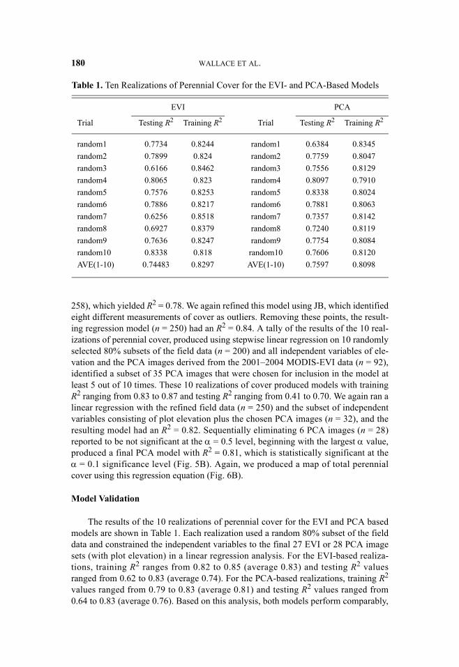
The results of the 10 realizations of perennial cover for the EVI and PCA basedmodels are shown in Table 1. Each realization used a random 80% subset of the fielddata and constrained the independent variables to the final 27 EVI or 28 PCA imagesets (with plot elevation) in a linear regression analysis. For the EVI-based realiza-tions, training R2 ranges from 0.82 to 0.85 (average 0.83) and testing R2 valuesranged from 0.62 to 0.83 (average 0.74). For the PCA-based realizations, training R2

values ranged from 0.79 to 0.83 (average 0.81) and testing R2 values ranged from0.64 to 0.83 (average 0.76). Based on this analysis, both models perform comparably,

Table 1. Ten Realizations of Perennial Cover for the EVI- and PCA-Based Models

EVI PCA

Trial Testing R2 Training R2 Trial Testing R2 Training R2

random1 0.7734 0.8244 random1 0.6384 0.8345 random2 0.7899 0.824 random2 0.7759 0.8047 random3 0.6166 0.8462 random3 0.7556 0.8129 random4 0.8065 0.823 random4 0.8097 0.7910 random5 0.7576 0.8253 random5 0.8338 0.8024 random6 0.7886 0.8217 random6 0.7881 0.8063 random7 0.6256 0.8518 random7 0.7357 0.8142 random8 0.6927 0.8379 random8 0.7240 0.8119 random9 0.7636 0.8247 random9 0.7754 0.8084 random10 0.8338 0.818 random10 0.7606 0.8120 AVE(1-10) 0.74483 0.8297 AVE(1-10) 0.7597 0.8098

PERENNIAL VEGETATION COVER DISTRIBUTION 181

with the EVI model having a slight edge in the training R2 and the PCA model anedge in the testing R2.

Figure 7 shows the mean and COV of the 10 perennial cover realizations for theEVI- and PCA-based models. These images were constructed to evaluate the stabilityof the models in space. In both the EVI and PCA models, the spatial distribution ofCOV shows that the models are very stable, with a COV < 0.5 over 90% of theMojave Desert. Higher values are found in parts of the Mojave Desert not representedby our field data, particularly areas of high cover or disturbance. These overall lowCOV values indicate that the model predictions are not overly influenced by theprecise subset of field data used to train the model. Furthermore, if our transect dataare representative of the Mojave Desert as a whole, then the COV values suggest thatthe model accuracy should be ±5% of the estimated cover value. Again, we found thatthe EVI and PCA models are comparable.

Fig. 7. Maps showing mean and coefficient of variation (COV, σ/μ) statistics at each pixel for10 realizations of perennial cover calculated by excluding 20% of the total perennial cover datafrom the linear regression. A. EVI model mean. B. EVI model COV. C. PCA model mean. D.PCA model COV.

182 WALLACE ET AL.

Predictive Strength of EVI Composites

For the EVI-based model, we explored the predictive strength of the 27 MODIS-EVI composites that were selected by the modeling process. Inspection of thesecomposites shows the relation of the annual composite date to perennial cover is com-plex—in some cases, the correlation coefficient changes sign depending on the year.For example, annual composite 2 (January 17 to February 2) is positively correlatedto total perennial cover in 2001 and 2002, but is negatively correlated in 2003 and2004. The highest correlations were obtained for composites from 2001, 2003, and2004. Although all four years are drought years, 2002 was exceptionally dry and hadvery little spring rain (Hereford et al., 2006). Most of the dominant perennial speciesin the Mojave are evergreen (e.g., Larrea tridentata), but a significant number ofco-dominants are drought deciduous. It is possible that the extreme drought centeredon 2002 altered the spectral signature of perennial vegetation compared to yearswith higher precipitation, an expected response particularly in the case of a drought-deciduous species.

The significant EVI composites occur throughout the year, and their ecologicalmeaning is not easy to determine. We expect perennial cover to be positively corre-lated to greenness when annuals are dormant (directly detecting perennials) but alsonegatively correlated to greenness when annuals are active (because annuals occupythe interstices between perennial plants). Such a simple relation is not obvious inthese data.

To partially unravel the complex contribution of individual EVI composites, wecompared these composites to desert-wide phenology (Fig. 8). Because EVI phenol-ogy changes with different landscapes, we stratified the area into an arbitrary 10regions using the unsupervised classification routine in ERDAS Imagine; thereforewe input the 92 EVI composites from January 2001 to December 2004 as a singlemulti-band image and specified an output of 10 clusters. Each image pixel is assignedto one of 10 clusters based on its particular EVI phenology and each cluster in themap (Fig. 8B) has the average phenology shown in the graph (Fig. 8A). This is thesame process we applied to the Landsat TM data to stratify the region into spectralclasses, but here we applied the process to MODIS data to produce classes with simi-lar phenologies.

As shown in Figure 8, the line-intercept data are represented in clusters 2 through8; cluster 10 is mostly agricultural land and cluster 1 is mostly barren. The 2002composites show no pulse of spring ephemerals, and clusters 2 through 9 are at aminimum during that year. Cluster 8 has an overall EVI value higher than cluster 7,but cluster 7 has a single strong peak in EVI in both the springs of 2001 and 2003 thatis earlier and stronger than the spring peak in cluster 8. Finally, clusters 5 and 6 havecomparable EVI values, but the EVI value of cluster 5 consistently increases earlier inthe spring. These differences likely reflect differing amounts and species compositionof vegetation contained in the landscapes, as well as phenological differences due toenvironmental factors, such as landscape position and substrate.

In Figure 8, individual composite dates that were selected for the final EVI modelare marked with vertical red lines (positive correlation) and black lines (negativecorrelation) at the top of the phenology graph. The lengths of the lines reflect the

PERENNIAL VEGETATION COVER DISTRIBUTION 183

absolute value of the coefficient, with long lines > 1.0. Figure 8 shows that the rela-tion among the composites and total perennial cover is too complex to easily explain,although there are some general trends, including: (1) extreme drought years (e.g.,2002) poorly reflect total perennial cover; (2) the strongest correlations are associatedwith summer composites in the more normal years; and (3) only weak correlations areassociated with the spring composites. To extract information to understand the rela-tion between specific annual composites and total perennial cover it may be necessaryto stratify the landscape into vegetation types or to limit analysis to a smaller geo-graphical region.

For the PCA-based model, the interpretation of the PC images selected by themodeling process is even more difficult. Table 2 summarizes the loadings matrix forthe 28 PC images used in the final PCA-based model. For each PC, we flagged theEVI bands with the highest loading values (using an arbitrary cutoff of ±0.200, except

Fig. 8. A. Average phenological profiles of MODIS-EVI values for 10 landscape clusters in theMojave Desert. The line-intercept locations used in the modeling occur in clusters 2 through 8.Vertical lines at the top of the EVI phenology profile show the individual composites (layers 1to 92 on the horizontal axis) that were selected for the final EVI-based model. Red and blacklines show composites with positive or negative correlations, respectively. Longer lines havecoefficients of absolute value 1.0 or greater. B: Map showing the spatial distribution of the 10Mojave landscape clusters.

184 WALLACE ET AL.

for PC1 where we allowed a lower threshold) and the sign (+ or –) of correlation. Foreach EVI band, we then tallied the number of flagged values. Finally, the flagged val-ues were tallied for each quarter of the year with Q1 = JFM, Q2 = AMJ, Q3 = JAS,and Q4 = OND. We found that most of the strong positive loadings occur in Q1 andQ2, whereas the negative loadings are dominant in Q1. Few significant loadingsoccur in 2002, a result reinforced by the EVI-based model results.

SUMMARY AND CONCLUSIONS

We used stepwise linear regression and simple linear regression analyses to createtwo models of total perennial cover for the Mojave Desert. In both models, the depen-dent data were measures of cover measured in the field using the line-interceptmethod. The independent data were plot elevation (included as a proxy for vegetationtype) and either MODIS-EVI data for 2001–2004 or principal component imagesderived from these data. We refined the models by first identifying and eliminating

Table 2. Summary of Loadings Matrix for Derived PCA Images Used in the Final PCA-Based Modela

Year Quarter No. of high loadings

Negative Positive Total

2001 Q1 11 7 18 2001 Q2 3 8 11 2001 Q3 3 3 6 2001 Q4 4 4 8 2002 Q1 4 4 8 2002 Q2 1 2 3 2002 Q3 2 1 3 2002 Q4 3 3 6 2003 Q1 2 5 7 2003 Q2 3 9 12 2003 Q3 3 5 8 2003 Q4 5 1 6 2004 Q1 13 8 21 2004 Q2 2 2 4 2004 Q3 1 0 1 2004 Q4 6 6 12

aFor each component, we flagged the EVI bands with the highest loading values (using an arbitrary cutoff of ± 0.200) and the sense (+ or –) of correlation. For each EVI band, we then tallied the number of flagged values. Finally, the flagged values were tallied for each quarter of the year with Q1 = JFM, Q2 = AMJ, Q3 = JAS, and Q4 = OND.

PERENNIAL VEGETATION COVER DISTRIBUTION 185

apparent outliers in the field data and then by evaluating the independent variables toidentify a subset that best predicts the measured cover.

Validation results and other checks of model stability and predictive powerrevealed that the models were indistinguishable from one another. For the data in thisapplication, it appears that the highly correlated nature of the MODIS-EVI compos-ites is not problematic, as they produce a similar result when compared to the PCAmodel that used uncorrelated data. Depending on the application, one model may beconsidered “better” than the other. The EVI-based model allows direct interpretationof the specific composite dates that correlate best to perennial cover, whereas inspec-tion of the PCA-based loadings reveal some paired couplets of positive/negativecorrelation that might reveal image ratios or differences that also correlate to cover.Nonetheless, the research shows that total perennial cover measured using the line-intercept technique at the plot level can be correlated with MODIS-EVI data and withPCA data derived from MODIS-EVI images, which allows estimation of total peren-nial cover over a much larger area than is represented by the plots.

Both models are spatially stable over most of the Mojave Desert, as indicatedby coefficients of variation (COV) calculated from an analysis of 10 realizationsproduced by randomly withholding 20% of the line-intercept data. Areas where addi-tional field data could be collected to improve the model are indicated by high COVvalues (Fig. 7). These areas tend to be in the high cover at higher elevations and inareas at greater distance from the line-intercept plots. In addition, based on an earlierpilot study at the Mojave National Preserve (C. S. A. Wallace, unpubl. data, 2002),the perennial vegetation model might be improved by stratifying the landscapeaccording to generalized vegetation type whenever a regional vegetation map isavailable.

This research demonstrates methods using standard commercial software fortaking large amounts of data, an ever-common situation, and winnowing them toselect useable and effective subsets—for example, by creating and evaluating a finiteset of realizations. This research also demonstrates that existing field data, collectedfor various campaigns and purposes, can be used effectively with remotely senseddata in modeling total perennial cover. Most projects that couple field and satellitedata oversee their own field campaign to collect data ideally suited to their project.Although this is an optimal approach, it is not always feasible or cost-effective—especially in regions already characterized by extensive historical datasets. In thiscase, we compiled existing data, screened them for suitable collection dates and com-parable field methods, and evaluated whether they were likely to be representative ofa 250 m MODIS pixel by characterizing the landscape complexity in the vicinity ofeach location with Landsat TM data.

The wealth of vegetation cover collected and compiled by U.S. GeologicalSurvey (USGS) personnel over the past century in the Mojave Desert offers an unpar-alleled opportunity for scientific investigations. This study represents a proof-of-concept for applying MODIS-EVI and field observations to estimating perennialcover throughout the Mojave Desert. Information on perennial cover provides detailsof vegetation distribution not captured by traditional vegetation maps. The resultingmap is an important enhancement to vegetation-distribution mapping that can be usedto inform several ongoing scientific investigations and management efforts related tothe vulnerability and recoverability of desert landscapes.

186 WALLACE ET AL.

ACKNOWLEDGMENTS

We thank Phil Leitner of the U.S. Fish and Wildlife Service and M. Hamilton ofFort Irwin for providing unpublished cover data for the western Mojave Desert andFort Irwin, respectively. Mimi Murov, the late Betsy Hobbs, and Keith Pohs contrib-uted greatly to USGS field data collection. We thank Dr. Susan Skirvin and Dr. BradReed for critically reviewing the manuscript. Feedback from Bruce Wylie was alsovaluable in strengthening the statistical approach used in this research. This researchwas supported by the Recoverability and Vulnerability of Desert Ecosystems Projectof the Priority Ecosystems Studies Program of the USGS.

REFERENCES

Bailey, R., 1995, Description of the Ecoregions of the United States, 2nd ed., Wash-ington, DC: U.S. Dept. of Agriculture, US. Forest Service.

Beatley, J. C., 1980, “Fluctuations and Stability in Climax Shrub and WoodlandVegetation of the Mojave, Great Basin, and Transition Deserts of SouthernNevada,” Israel Journal of Botany, 28:149–168.

Brondizio, E. S., Moran, E. F., Mausel, P., and Y. Wu, 1994, “Land Use Change in theAmazon Estuary: Patterns of Caboclo Settlement and Landscape Management,”Human Ecology, 22(3):249–278.

Chen, Z. M., Babiker, I. S., Chen, Z. X., Komaki, K., Mohamed, M. A. A., andK. Kato, 2004, “Estimation of Interannual Variation in Productivity of GlobalVegetation Using NDVI Data,” International Journal of Remote Sensing,25(16):3139–3159.

Cohen, W. B., Maiersperger, T. K., Gower, S. T., and D. P. Turner, 2003, “AnImproved Strategy for Regression of Biophysical Variables and Landsat ETM+Data,” Remote Sensing of Environment, 84:561–571.

Camacho-De Coca, F., García-Haro, F. J., Gilabert, M. A., and J. Meliá, J., 2004,“Vegetation Cover Seasonal Changes Assessment from TM Imagery in a Semi-arid Landscape,” International Journal of Remote Sensing, 25(17):3451–3476.

Fox, J., 2002, An R and S-Plus Companion to Applied Regression, Thousand Oaks,CA: Sage Publications.

Hansen, M. C., DeFries, R. S., Townsend, J. R. G., Sohlberg, R. A., Dimiceli, C., andC. Carroll, 2002, “Towards an Operational MODIS Continuous Field of PercentTree Cover Algorithm: Examples Using AVHRR and MODIS Data,” RemoteSensing of Environment, 83(1):303–319.

Hansen, M. C., Townshend, R. G., DeFries, R.., and M. Carroll, 2005, “Estimation ofTree Cover Using MODIS Data at Global, Continental, and Regional/LocalScales,” International Journal of Remote Sensing, 26(19):4359–4380.

Hereford, R., Webb, R. H., and C. Longpré, 2006, “Precipitation History and Ecosys-tem Response to Multidecadal Precipitation Variability in the Mojave Desert andVicinity, 1893–2001,” Journal of Arid Environments, 67:13–34.

Huete, A. R., 1988, “A Soil-Adjusted Vegetation index (SAVI),” Remote Sensing ofEnvironment, 25(3):295–309.

PERENNIAL VEGETATION COVER DISTRIBUTION 187

Huete, A. R., Didan, K., Miura, T., Rodriguez, E. P., Gao, X., and L. G. Ferreira, 2002,“Overview of the Radiometric and Biophysical Performance of the MODISVegetation Indices,” Remote Sensing of Environment, 83:195–213.

Jensen, J. R., 1996, Introductory Digital Image Processing: A Remote SensingPerspective, Upper Saddle River, NJ: Prentice Hall, 318 p.

Jensen, J. R., 2000, Remote Sensing of the Environment: An Earth Resource Perspec-tive, Upper Saddle River, NJ: Prentice Hall, 544 p.

Lovich, J. E. and D. Bainbridge, 1999, “Anthropogenic Degradation of the SouthernCalifornia Desert Ecosystem and Prospects for Natural Recovery and Restora-tion,” Environmental Management, 24:309–326.

Lowry, J. H, Jr., Ramsey, R. D., Thomas, K. A., Schrupp, D., Sajwaj, T., Kirby, J.,Waller, E., Schrader, S., Falzarano, S. Langs, L., Manis, G., Wallace, C., Schulz,K., Comer, P., Pohs, K., Rieth, W., Velasquez, C., Wolk, B., Kepner, W., Boykin,K., O’Brien, L., Bradford, D., Thompson, B., and J. Prior-Magee, 2007, “Map-ping Moderate-Scale Land-Cover over Very Large Geographic Areas within aCollaborative Framework: A Case Study of the Southwest Regional Gap Analy-sis Project (SWReGAP),” Remote Sensing of Environment, 108:59–73.

Ostler, W. K., Hansen, D. J., Anderson, D. C., and D. B. Hall, 2000, Classification ofVegetation on the Nevada Test Site, Las Vegas, NV: U.S. Department of Energy,Nevada Operations Office, Report DOE/NV/11718-477.

Peterson, E. B., 2005, “Estimating Cover of an Invasive Grass (Bromus tectorum)Using Tobit Regression and Phenology Derived from Two Dates of LandsatETM+ Data,” International Journal of Remote Sensing, 26:2491–2507.

Quinlan, J. R., 1996, “Bagging, Boosting, and C4.5,” in Proceedings of the 13 AAAIConference on Artificial Intelligence, Menlo Park, CA: AAAI Press, 725–730.

Rahman, M. M., Csaplovics, E., and B. Koch, 2005, “An Efficient Regression Strat-egy for Extracting Forest Biomass Information from Satellite Sensor Data,”International Journal of Remote Sensing, 26:1511–1519.

Thomas, K., Keeler-Wolf, T., Franklin, J., P. Stine, 2004, Mojave Desert EcosystemProgram: Central Mojave Vegetation Database, Sacramento, CA: U.S. Geologi-cal Survey, Western Ecological Research Center Report.

Tucker, C. J., Townshend, J. R. G., and T. E. Goff, 1985, “African Land-Cover Classi-fication Using Satellite Data,” Science, 227:369–375.

Webb, R. H., Murov, M. B., Esque, T. C., Boyer, D. E., DeFalco, L. A., Haines, D. F.,Oldershaw, D., Scoles, S. J., Thomas, K. A., Blainey, J. B., and P. A. Medica,2003, Perennial Vegetation Data from Permanent Plots on the Nevada Test Site,Nye County, Nevada, Washington, DC: U.S. Geological Survey Open-File Report03-336.

Webb, R. H., Steiger, J. W., and E. B. Newman, 1988, The Effects of Disturbance onDesert Vegetation in Death Valley National Monument, California, Washington,DC: U.S. Geological Survey Bulletin 1793.

Wulder, M. A., 2005, “A Practical Guide to the Use of Selected Multivariate Statis-tics,” Canadian Forest Service [www.pfc.forestry.ca/profiles/wulder/mvstats/index_e.html].

Wulder, M. A. and S. E. Franklin, 2003, Remote Sensing of Forest Environments:Concepts and Case Studies, Boston, MA: Kluwer Academic Publishers.