
Remote sensing the spatial and temporal structure of
93
JOURNAL OF GEOPHYSICAL RESEARCH, VOL. ???, XXXX, DOI:10.1029/, Remote sensing the spatial and temporal structure of 1 magnetopause and magnetotail reconnection from 2 the ionosphere 3 G. Chisham, 1 M. P. Freeman, 1 G. A. Abel, 1 M. M. Lam, 1 M. Pinnock, 1 I. J. Coleman, 1 S. E. Milan, 2 M. Lester, 2 W. A. Bristow, 3 R. A. Greenwald, 4 G. J. Sofko, 5 J.-P. Villain, 6 G.Chisham, M.P.Freeman, G.A.Abel, M.M.Lam, M. Pinnock, I.J.Coleman, British Antarc- tic Survey, Natural Environment Research Council, High Cross, Madingley Road, Cambridge, CB3 0ET, United Kingdom. ([email protected], [email protected], [email protected], [email protected], [email protected]) S.E.Milan, M.Lester, Department of Physics and Astronomy, University of Leicester, Leicester, LE1 7RH, United Kingdom. W.A.Bristow, UAF Geophysical Institute, 903 Koyukuk Drive, Fairbanks, Alaska 99775, USA. R.A.Greenwald, Applied Physics Laboratory, Johns Hopkins University, Laurel, MD 20723, USA. G.J.Sofko, University of Saskatchewan, 116 Science Place, Saskatoon, Saskatchewan, S7N 5E2, Canada. J.-P.Villain, LPCE/CNRS, 3A, Avenue de la recherche Scientifique, Orleans, 45071, France. 1 British Antarctic Survey, Natural DRAFT September 7, 2007, 3:34pm DRAFT
-
Upload
antarctica -
Category
Documents
-
view
3 -
download
0
Transcript of Remote sensing the spatial and temporal structure of

JOURNAL OF GEOPHYSICAL RESEARCH, VOL. ???, XXXX, DOI:10.1029/,
Remote sensing the spatial and temporal structure of1
magnetopause and magnetotail reconnection from2
the ionosphere3
G. Chisham,1
M. P. Freeman,1
G. A. Abel,1
M. M. Lam,1
M. Pinnock,1
I. J.
Coleman,1
S. E. Milan,2
M. Lester,2
W. A. Bristow,3
R. A. Greenwald,4
G. J.
Sofko,5
J.-P. Villain,6
G.Chisham, M.P.Freeman, G.A.Abel, M.M.Lam, M. Pinnock, I.J.Coleman, British Antarc-
tic Survey, Natural Environment Research Council, High Cross, Madingley Road, Cambridge,
CB3 0ET, United Kingdom. ([email protected], [email protected], [email protected], [email protected],
S.E.Milan, M.Lester, Department of Physics and Astronomy, University of Leicester, Leicester,
LE1 7RH, United Kingdom.
W.A.Bristow, UAF Geophysical Institute, 903 Koyukuk Drive, Fairbanks, Alaska 99775, USA.
R.A.Greenwald, Applied Physics Laboratory, Johns Hopkins University, Laurel, MD 20723,
USA.
G.J.Sofko, University of Saskatchewan, 116 Science Place, Saskatoon, Saskatchewan, S7N 5E2,
Canada.
J.-P.Villain, LPCE/CNRS, 3A, Avenue de la recherche Scientifique, Orleans, 45071, France.
1British Antarctic Survey, Natural
D R A F T September 7, 2007, 3:34pm D R A F T
X - 2 CHISHAM ET AL.: REMOTE SENSING OF RECONNECTION
Abstract. Magnetic reconnection is the most significant process that re-4
sults in the transport of magnetised plasma into, and out of, the Earth’s magnetosphere-5
ionosphere system. There is also compelling observational evidence that it6
plays a major role in the dynamics of the solar corona, and it may also be7
Environment Research Council, High Cross,
Madingley Road, Cambridge, CB3 0ET,
United Kingdom.
2Department of Physics and Astronomy,
University of Leicester, Leicester, LE1 7RH,
United Kingdom.
3UAF Geophysical Institute, 903 Koyukuk
Drive, Fairbanks, Alaska 99775, USA.
4Applied Physics Laboratory, Johns
Hopkins University, Laurel, MD 20723,
USA.
5University of Saskatchewan, 116 Science
Place, Saskatoon, Saskatchewan, S7N 5E2,
Canada.
6LPCE/CNRS, 3A, Avenue de la
recherche Scientifique, Orleans, 45071,
France.
D R A F T September 7, 2007, 3:34pm D R A F T

CHISHAM ET AL.: REMOTE SENSING OF RECONNECTION X - 3
important for understanding cosmic rays, accretion disks, magnetic dynamos,8
and star formation. The Earth’s magnetosphere and ionosphere are presently9
the most accessible natural plasma environments where magnetic reconnec-10
tion and its consequences can be measured, either in situ, or by remote sens-11
ing. This paper presents a complete methodology for the remote sensing of12
magnetic reconnection in the magnetosphere from the ionosphere. This method13
combines measurements of ionospheric plasma convection and the ionospheric14
footprint of the reconnection separatrix. Techniques for measuring both the15
ionospheric plasma flow and the location and motion of the reconnection sep-16
aratrix are reviewed, and the associated assumptions and uncertainties as-17
sessed, using new analyses where required. Application of the overall method-18
ology is demonstrated by the study of a 2-hour interval from 26 December19
2000 using a wide range of spacecraft and ground-based measurements of the20
northern hemisphere ionosphere. This example illustrates how spatial and21
temporal variations in the reconnection rate, as well as changes in the bal-22
ance of magnetopause (dayside) and magnetotail (nightside) reconnection,23
can be routinely monitored, affording new opportunities for understanding24
the universal reconnection process and its influence on all aspects of space25
weather.26
D R A F T September 7, 2007, 3:34pm D R A F T

X - 4 CHISHAM ET AL.: REMOTE SENSING OF RECONNECTION
1. Introduction
It has been estimated that over 99.99% of the universe is made up of plasma - the fourth27
state of matter, composed of free ions and electrons. Despite its universal importance, our28
understanding of natural plasmas is limited by our ability to observe their behaviour and29
measure their properties. The most accessible natural plasma environment for study is30
the Earth’s magnetosphere-ionosphere system. The Earth’s magnetosphere is that region31
of near-Earth space which is permeated by the Earth’s magnetic field. The plasma in the32
magnetosphere is controlled mainly by magnetic and electric forces that are much stronger33
here than gravity or the effect of collisions. The magnetosphere is embedded in the34
outflowing plasma of the solar corona, known as the solar wind, and its associated magnetic35
field, the interplanetary magnetic field (IMF). Because of the high conductivity of the36
solar wind and magnetospheric plasmas, their respective magnetic fields are effectively37
“frozen-in” to the plasma (like in a superconductor). The frozen-in nature of these two38
plasmas means that the solar wind cannot easily penetrate the Earth’s magnetic field39
but is mostly deflected around it. This results in the distortion of the magnetosphere40
and the two plasmas end up being separated by a boundary, the magnetopause. The41
magnetopause is roughly bullet-shaped and extends to ∼10-12 Earth radii (RE) on the42
dayside of the Earth, and stretches out into a long tail, the magnetotail, which extends to43
hundreds of RE on the nightside of the Earth. However, the two plasma regions are not44
totally isolated as the process of magnetic reconnection allows the transmission of solar45
wind mass, energy, and momentum across the magnetopause, and into the magnetosphere.46
D R A F T September 7, 2007, 3:34pm D R A F T

CHISHAM ET AL.: REMOTE SENSING OF RECONNECTION X - 5
Magnetic reconnection (or merging) is a physical process [Priest and Forbes, 2000] which47
involves a change in the connectivity of magnetic field lines (or magnetic flux) that fa-48
cilitates the transfer of mass, momentum and energy. The resultant splicing together49
of different magnetic domains changes the overall topology of the magnetic field. If we50
consider a magnetic topology with antiparallel magnetic field lines frozen into two adjoin-51
ing plasmas, where the plasma and magnetic field lines on both sides are moving toward52
each other, this results in a current sheet separating these regions, with a large change53
in the magnetic field across it. The frozen-in field approximation breaks down in this54
current sheet allowing magnetic field lines to diffuse across the plasma. This diffusion55
allows oppositely-directed magnetic fields to annihilate at certain points. This results in56
X-type configurations of the magnetic field, as shown in the schematic representation of57
a two-dimensional reconnection region in fig.1. Here, the magnetic field strength is zero58
at the centre of the X, termed the magnetic neutral point. The magnetic field lines form-59
ing the X, and passing through the neutral point, are called the separatrix. Plasma and60
magnetic field lines are transported toward the neutral point from either side as shown61
by the blue arrows in fig.1. Reconnection of the field lines occurs at the neutral point62
and the merged field lines, populated by a mixture of plasma from both regions, are ex-63
pelled from the neutral point approximately perpendicular to their inflow direction. This64
process of magnetic reconnection is fundamental to the behaviour of the natural plasmas65
of many astrophysical environments. For example, solar flares, the largest explosion in66
the solar system, are caused by the reconnection of large systems of magnetic flux on the67
Sun, releasing in minutes the energy that has been stored in the solar magnetic field over68
a period of weeks to years. Reconnection is also important to the science of controlled69
D R A F T September 7, 2007, 3:34pm D R A F T

X - 6 CHISHAM ET AL.: REMOTE SENSING OF RECONNECTION
nuclear fusion as it is one mechanism preventing the magnetic confinement of the fusion70
fuel.71
At the Earth’s magnetopause magnetic reconnection is the major process through which72
solar wind mass, energy and momentum are transferred from the solar wind into the73
magnetospheric system. Together with reconnection within the magnetotail, this drives a74
global circulation of plasma and magnetic flux within the magnetosphere and ionosphere75
[Dungey, 1961]. Figure 2 presents a schematic representation of the magnetosphere in76
the noon-midnight meridian plane which highlights the topology of the Earth’s magnetic77
field and its connection to the IMF. Point N1 marks an example location of a reconnection78
neutral point on the dayside magnetopause, with an IMF field line (marked 1) reconnecting79
with a geomagnetic field line (marked 1′). Typically, the connectivity of geomagnetic field80
lines is of two types: Open - one end of the magnetic field line is connected to the Earth,81
the other to the IMF. Closed - both ends are connected to the Earth. Geomagnetic field82
line 1′ represents the last closed field line in the dayside magnetosphere. As a result of83
the magnetopause reconnection two open field lines are created (marked 2 and 2′) which84
are dragged by the solar wind flow to the nightside of the magnetosphere and into the85
magnetotail (to points 3 and 3′). Here, the existence of the anti-parallel magnetic field86
configuration results in magnetotail reconnection (at neutral point N2 in fig.2). In three87
dimensions, the reconnection X-points depicted as N1 and N2 in fig.2 are thought to88
extend along the magnetopause and magnetotail current sheets in lines known as X-lines.89
Figure 3 presents a 3-dimensional schematic representation of the magnetosphere which90
highlights these extended X-lines.91
D R A F T September 7, 2007, 3:34pm D R A F T

CHISHAM ET AL.: REMOTE SENSING OF RECONNECTION X - 7
Accurate measurement of both the magnetopause and magnetotail reconnection rates,92
and an understanding of the factors that influence them has been a major scientific goal93
for many years. The reconnection rate (or equivalently the reconnection electric field)94
is defined as the rate of transfer of magnetic flux across unit length of the separatrix95
between the unreconnected and reconnected field lines. In the magnetospheric environ-96
ment, important outstanding questions concerning reconnection, which can be addressed97
by reconnection rate measurements, include: Where is the typical location, and what is98
the typical extent (in both time and space), of both the magnetopause and magneto-99
tail X-lines? How does the reconnection rate vary along these X-lines, and with time?100
How do these things change with changing interplanetary magnetic field and geomagnetic101
conditions?102
The reconnection rate can be measured by spacecraft in the reconnecting current sheet,103
local to the neutral points, by measuring the electric field tangential to the reconnection X-104
line [Sonnerup et al., 1981; Lindqvist and Mozer, 1990]. Such studies have shown evidence105
for a fast reconnection rate (inflow speed / Alfven speed ∼ 0.1) [Priest and Forbes, 2000].106
However, it is generally difficult to measure the reconnection rate with satellites because107
it must be measured in the frame of reference of the separatrix, which is often in motion.108
Hence, such measurements are typically sparse in space and time, limited to the location109
and time of each spacecraft crossing of the current sheet.110
More continuous and extensive measurements of reconnection in time and space can111
presently be achieved only by remotely sensing magnetic reconnection in the magneto-112
sphere from the ionosphere. The ionosphere, located at altitudes of ∼80-2000 km, forms113
the base of the magnetospheric plasma environment. It is the transition region from the114
D R A F T September 7, 2007, 3:34pm D R A F T
X - 8 CHISHAM ET AL.: REMOTE SENSING OF RECONNECTION
fully-ionized magnetospheric plasma to the neutral atmosphere of the Earth. As can be115
seen in fig.3, the focussing effect of the Earth’s dipole-like magnetic field projects recon-116
nection signatures from the vast volume of the magnetosphere onto the relatively small117
area of the polar ionospheres, where they can be measured by ground- and space-based118
instruments. Hence, the ionospheric perspective is immensely valuable as a window to119
the huge outer magnetosphere and the reconnection processes occurring there.120
In simple quasi-steady-state reconnection scenarios for different IMF orientations121
[Dungey, 1961, 1963; Russell, 1972; Cowley, 1981], and in the absence of other (e.g.,122
viscous) transport processes [Axford and Hines, 1961], the total globally-integrated re-123
connection rate is equal to the maximum electric potential difference across the polar124
ionosphere. This can be measured every ∼100 min by low-altitude polar-orbiting satel-125
lites [Reiff et al., 1981] or at higher cadence by ground-based radar and magnetometer126
networks [Ruohoniemi and Baker, 1998; Richmond and Kamide, 1988]. Such studies have127
investigated the functional dependence of the integrated reconnection rate on the relative128
orientation of the reconnecting magnetic fields [Reiff et al., 1981; Freeman et al., 1993].129
More generally, imbalance of the integrated reconnection rates at the magnetopause130
and in the magnetotail results in a change in the relative proportions of open and closed131
magnetic flux [Siscoe and Huang, 1985; Cowley and Lockwood, 1992]. Thus, for unbalanced132
reconnection, the difference in the two integrated reconnection rates can be measured from133
the rate of change of polar cap area (the area of incompressible open magnetic flux that134
threads the polar ionospheres). Estimates of both the magnetopause and magnetotail135
reconnection rates can then be made whenever one or the other reconnection rate can136
be estimated [Lewis et al., 1998], or is negligible [Milan et al., 2003], or by summing the137
D R A F T September 7, 2007, 3:34pm D R A F T

CHISHAM ET AL.: REMOTE SENSING OF RECONNECTION X - 9
difference measurement with an estimate of the average of the two reconnection rates given138
by the cross-polar cap potential [Cowley and Lockwood, 1992]. Such studies have revealed139
and quantified the variation of global magnetopause and magnetotail reconnection through140
the substorm cycle [Milan et al., 2007].141
On shorter time scales, local reconnection rates have been inferred from low-altitude142
spacecraft observations of the dispersion of ions from the reconnection site precipitating143
into the ionosphere on newly-opened magnetic field lines [Lockwood and Smith, 1992].144
These observations provide a temporal profile of the reconnection rate at a single location145
for the duration of the satellite pass (∼10 min). Such studies show the reconnection rate146
to vary on timescales of minutes, as suggested by the in-situ observation of flux transfer147
events (instances of transient reconnection) at the magnetopause [Russell and Elphic,148
1978].149
Most generally, the reconnection rate is measured from the ionosphere by first detect-150
ing the ionospheric projections of regions of different magnetic connectivity (e.g., open151
and closed magnetospheric field lines) and then measuring the transport of magnetic flux152
between them. The reconnection rate equates to the component of the ionospheric convec-153
tion electric field tangential to the ionospheric projection of the reconnection separatrix,154
in the frame of the reconnection separatrix. Hence, in a ground-based measurement frame,155
contributions can arise from (1) plasma convecting across the separatrix, and (2) move-156
ment of the separatrix in the measurement frame. As shown schematically in fig.3, the157
reconnection separatrix (yellow and green shaded areas) maps down magnetic field lines158
from the in-situ reconnection X-lines (bold blue lines in space) to regions in the polar iono-159
spheres termed “merging lines” (bold blue lines in the ionosphere). The different magnetic160
D R A F T September 7, 2007, 3:34pm D R A F T

X - 10 CHISHAM ET AL.: REMOTE SENSING OF RECONNECTION
field topologies in the two regions either side of the separatrix give rise to different plasma161
properties in each region, which can be detected at the ionospheric footprints. During162
southward IMF conditions, when magnetopause reconnection occurs preferentially on the163
low-latitude magnetopause (as in figs.2 and 3), the dayside merging line is co-located164
with the ionospheric projection of the open-closed magnetic field line boundary (OCB),165
alternatively termed the polar cap boundary. During strong northward IMF conditions,166
when reconnection occurs at high latitudes on the magnetotail lobe magnetopause, the167
reconnection separatrix is typically located some distance poleward of the OCB, within168
the polar cap, at the point where the lobe magnetopause maps into the ionosphere. On169
the nightside of the Earth the merging line associated with the most-distant magnetotail170
X-line is always co-located with the OCB. Reconnection is also thought to occur Earth-171
ward of this far-tail X-line (at a near-Earth neutral line) but there is not as yet a clear172
signature of the ionospheric projection of this X-line.173
The first reconnection rate measurements of this type were made in the nightside iono-174
sphere by de la Beaujardiere et al. [1991] using Sondrestrom Incoherent Scatter Radar175
(ISR) measurements. Using a single meridional radar beam they measured the plasma176
velocity across the OCB in the OCB rest frame. The location of the OCB was estimated177
by identifying strong electron density gradients which occur at ionospheric E-region al-178
titudes along the poleward boundary of the auroral oval. These are thought to be a179
good proxy for the OCB in the nightside ionosphere. Blanchard et al. [1996, 1997] later180
refined these measurements by locating the OCB using both E-region electron density181
measurements and 630 nm auroral emissions measured by ground-based optical instru-182
ments. They investigated how the magnetotail reconnection rate varied with magnetic183
D R A F T September 7, 2007, 3:34pm D R A F T

CHISHAM ET AL.: REMOTE SENSING OF RECONNECTION X - 11
local time, with variations in the IMF, and with substorm activity. Since then, a number184
of studies have used single radar beams to make single-point reconnection rate measure-185
ments of this type in both the dayside and nightside ionospheres [Pinnock et al., 1999;186
Blanchard et al., 2001; Østgaard et al., 2005]. These studies have used a range of different187
techniques to determine the OCB location and motion. However, the employment of a188
single meridional radar beam in the above studies meant that no investigation could be189
made of spatial variations in the reconnection rate.190
Baker et al. [1997] first measured the reconnection rate across an extended longitudinal191
region. They used the technique of L-shell fitting [Ruohoniemi et al., 1989] to estimate192
two-dimensional ionospheric convection velocity vectors from line-of-sight velocity mea-193
surements made by a single radar of the Super Dual Auroral Radar Network (SuperDARN)194
[Greenwald et al., 1995; Chisham et al., 2007]. They also used variations in the Doppler195
spectral width characteristics measured by the radar to estimate the OCB location. Since196
then, the advent of large networks of ionospheric radars which can measure the plasma197
convection velocity over large regions of the ionosphere has made extensive measurements198
of the reconnection rate a reality. Recent studies [Pinnock et al., 2003; Milan et al.,199
2003; Chisham et al., 2004b; Hubert et al., 2006; Imber et al., 2006] have employed the200
technique of SuperDARN global convection mapping to measure the convection velocity201
across large regions of the polar ionospheres for a range of IMF conditions. Combined with202
measurements of the location and motion of the ionospheric footprint of the reconnection203
separatrix from a range of different instrumentation, these studies have illustrated that204
the magnetopause reconnection rate not only varies with time but also with longitudinal205
D R A F T September 7, 2007, 3:34pm D R A F T

X - 12 CHISHAM ET AL.: REMOTE SENSING OF RECONNECTION
location along the merging line. The magnetotail reconnection rate has also been studied206
in a similar way [Lam et al., 2006; Hubert et al., 2006].207
The purpose of this paper is to build on these previous studies and to present a standard208
methodology for reconnection rate determination which can be easily implemented. To209
this end we:210
(1) Set out in full a complete methodology for remote sensing of the reconnection rate.211
(2) Review the techniques for determining the ionospheric convection velocity field and212
the ionospheric projection of the reconnection separatrix.213
(3) Highlight and discuss problems and uncertainties concerning the methodology and214
techniques.215
(4) Present an example of a global application of this methodology.216
2. Methodology for estimating the reconnection rate
In this section we outline mathematically the methodology for determining reconnection217
rates using ionospheric measurements. We also review the instrumentation and analysis218
techniques used to make these ionospheric measurements. The application of many of219
these techniques is described by considering a 2-hour interval of data from 26 December220
2000. The results of the reconnection rate analysis using the combined data sets from this221
interval are presented in section 3.222
2.1. Theory
2.1.1. General formulation223
The principle of remote measurement of the reconnection electric field was first pre-224
sented by Vasyliunas [1984] who argued that the potential variation along the ionospheric225
D R A F T September 7, 2007, 3:34pm D R A F T

CHISHAM ET AL.: REMOTE SENSING OF RECONNECTION X - 13
projection of the reconnection separatrix (the merging line) related directly to that along226
the in-situ reconnection X-line. The reconnection electric field in the ionosphere equates227
to the component of the ionospheric convection electric field that is directed tangential to228
the ionospheric projection of the reconnection separatrix, in the frame of the separatrix.229
This equates to the rate of flux transfer across the reconnection separatrix, assuming that230
the magnetic field is frozen in to the plasma. It is assumed that the plasma flow in the231
polar ionosphere is dominated by the convection electric field and that the convection232
velocity field is divergence-free.233
The reconnection rate, or electric field (Erec), in the ionosphere at any point s along234
the reconnection separatrix at a time t can be written235
Erec(s, t) = E′(s, t) · T(s, t) (1)236
where E′(s, t) is the convection electric field at the separatrix, in the frame of the separa-237
trix, and238
T(s, t) =dP(s, t)
ds(2)239
represents the tangent to the separatrix, where P(s, t) describes the location of the sepa-240
ratrix.241
We can relate the convection electric field to the ionospheric convection velocity field if242
we assume the ideal magnetohydrodynamic approximation of Ohm’s law243
E′(s, t) = −(V′(s, t) × B(s)) (3)244
where V′(s, t) is the convection velocity at locations along the separatrix, in the frame of245
the separatrix (a one-dimensional path through the convection velocity field V′(x, t)), and246
B(s) = Bz(s)z is the magnetic field (approximated as being vertical and time invariant).247
D R A F T September 7, 2007, 3:34pm D R A F T
X - 14 CHISHAM ET AL.: REMOTE SENSING OF RECONNECTION
The normal to the separatrix at a fixed ionospheric height can be written as,248
N(s, t) = −(z × T(s, t)) (4)249
and hence, combining (1), (3), and (4), the reconnection electric field, (1), can be rewritten250
as,251
Erec(s, t) = Bz(s)(V′(s, t) · N(s, t)
)(5)252
The ionospheric convection velocity is not typically measured in the frame of the sep-253
aratrix and hence we need to convert convection velocity measurements V(s, t) into this254
frame using the transformation,255
V′(s, t) = V(s, t) − dP(s, t)
dt(6)256
By combining (5) and (6) we can write the reconnection electric field as,257
Erec(s, t) = Bz(s)
[(V(s, t) − dP(s, t)
dt
)· N(s, t)
](7)258
The total rate of flux transfer (dF12(t)/dt) along a merging line connecting points P1259
and P2 is given by the integrated reconnection rate, or reconnection voltage (φ12(t)), which260
is determined by integrating the reconnection electric field along this merging line.261
φ12(t) =dF12(t)
dt262
=∫ P2
P1
Erec(s, t) ds263
=∫ P2
P1
Bz(s)
[(V(s, t) − dP(s, t)
dt
)· N(s, t)
]ds (8)264
Typically, reconnection at the magnetopause increases open magnetic flux whereas265
reconnection in the magnetotail decreases open flux. Consequently the total globally-266
integrated reconnection rate in the magnetospheric system is given by the rate of change267
D R A F T September 7, 2007, 3:34pm D R A F T

CHISHAM ET AL.: REMOTE SENSING OF RECONNECTION X - 15
of open magnetic flux in the polar cap268
dFpc
dt= Bi
dApc
dt= φd + φn (9)269
where φd and φn are the total reconnection voltages along the magnetopause and magne-270
totail X-lines, respectively, and Apc is the area of open flux in the ionosphere. Measuring271
the reconnection rate from the ionosphere offers the advantages that Apc is minimized272
and Bi is approximately constant and hence can be described by a static empirical model.273
Thus, by measuring changes in polar cap area, the measurement of either of the magne-274
topause or magnetotail reconnection voltages allows estimation of the other [Milan et al.,275
2003].276
2.1.2. Discrete formulation277
Actual measurements of the convection velocity (V) and the reconnection separatrix278
position in the ionosphere (P) typically comprise sparse discrete observations, rather than279
continuous functions. Consequently, for practical purposes we rewrite (7) in a discrete280
form as,281
Ereci(t) = Bzi
[(Vi(t) − VPi
(t)) · Ni(t)]
(10)282
where subscript i refers to a discrete velocity vector measurement and where the motion283
of the separatrix has been simplified as VPi(the meridional component of the separatrix284
velocity at the location of velocity vector i). For ease of calculation we rewrite this as,285
Ereci(t) = Bzi
[|Vi(t)| cos θi(t) − |VPi(t)| cosαi(t)] (11)286
where θi is the angle between the velocity vector and the normal to the separatrix and αi287
is the angle between the meridional direction and the normal to the separatrix. Hence,288
estimates of the reconnection rate require measurements of the vertical magnetic field289
D R A F T September 7, 2007, 3:34pm D R A F T

X - 16 CHISHAM ET AL.: REMOTE SENSING OF RECONNECTION
strength, the separatrix location and motion, and the convection velocity. The magnetic290
field strength varies little in the incompressible ionosphere and so values from the Altitude-291
Adjusted Corrected Geomagnetic (AACGM) field model [Baker and Wing, 1989] can be292
assumed. The AACGM model is also used as the geomagnetic coordinate system in this293
analysis.294
Generally, our discrete measured velocity vectors will not be co-located with the mea-295
sured separatrix location. Hence, we consider velocity vectors close to the separatrix to296
be the best estimate of the velocity field at the separatrix. Typically, those within half297
the latitudinal resolution of the velocity measurements are most suitable. Fig.4 presents298
a basic schematic representation of the scenario at each discrete measurement point i.299
Figure 4a presents an example scenario of the actual measured quantities. We have suit-300
able velocity vectors Vi = V(λi, φi) at N discrete locations with AACGM latitude λi301
and AACGM longitude φi (i = 1...N) and separatrix identifications Pj = P(λj, φj) at302
M discrete positions with AACGM latitude λj and AACGM longitude φj (j = 1...M).303
Figure 4b shows the derived quantities that are used as input to equation (11) for the304
same example as in fig.4a. For each velocity vector we assume that the measured velocity305
is a good approximation for the velocity at the separatrix at the same AACGM longitude.306
Pi is an estimate of the separatrix position at AACGM longitude φi, the latitude of which307
can be approximated by the linear interpolation of neighbouring separatrix measurements308
(λj1, φj1) and (λj2, φj2),309
λ(Pi) = λj1 +
(λj2 − λj1
φj2 − φj1
)(φi − φj1) (12)310
If the discrete separatrix points are not too far apart then we can assume a locally linear311
approximation. Therefore, the angle αi = α(Pi) between the normal to the separatrix312
D R A F T September 7, 2007, 3:34pm D R A F T

CHISHAM ET AL.: REMOTE SENSING OF RECONNECTION X - 17
and the meridional direction can be given as,313
αi = tan−1
[λj2 − λj1
(φj2 − φj1) cosλj2
]. (13)314
Alternatively, λ(Pi) and αi can be estimated by a higher order method (see section 2.3.6).315
The angle between the velocity vector Vi and the meridian direction is given by θVi=316
θV(λi, φi). Hence, the angle between the velocity vector and the normal to the separatrix317
is given by,318
θi = θVi− αi (14)319
We assume for simplicity that the separatrix motion in the ionosphere is purely latitu-320
dinal and hence the magnitude of the separatrix velocity at AACGM longitude φi is given321
by,322
|VPi(t)| =
(RE + h) [λ(Pi(t)) − λ(Pi(t− Δt))]
Δt(15)323
where RE is the radius of the Earth, h is the altitude of the observations, and Δt is the324
time between successive separatrix estimates.325
Entering single point measurements into (11) allows us to make localised estimates of326
the reconnection electric field [Pinnock et al., 1999; Blanchard et al., 2001]. However, if we327
wish to determine the spatiotemporal structure of the electric field or make an estimate of328
the reconnection voltage along a merging line, we need to make as many measurements as329
possible along the merging line. If we assume Nvec discrete velocity vector measurements330
along a merging line, the total rate of flux transfer, or reconnection voltage, for that331
merging line can be estimated from,332
φrec(t) =Nvec∑i=1
Ereci(t) Δsi(t) (16)333
D R A F T September 7, 2007, 3:34pm D R A F T

X - 18 CHISHAM ET AL.: REMOTE SENSING OF RECONNECTION
where Δsi(t) represents the length of the separatrix portion at measurement location i,334
which for closely-spaced measurements can be approximated by,335
Δsi(t) ≈( |Pi+1(t) − Pi−1(t)|
2
)(17)336
2.1.3. Error analysis337
In order to gain a quantitative feel for reconnection rate estimates we need to have an338
appreciation of the uncertainties in the measured quantities. We can estimate the uncer-339
tainty, or error, in a single measurement of the reconnection electric field at measurement340
point i as,341
ε〈Ereci(t)〉 ≈ Bzi
(ε〈|Vi(t)| cos θi(t)〉2 + ε〈|VPi
(t)| cosαi(t)〉2) 1
2 (18)342
where ε〈x〉 represents the uncertainty in the measurement of parameter x. (This rep-343
resentation assumes that the uncertainty in the magnetic field (ε〈Bzi〉) is negligible.)344
This uncertainty should only be viewed as an estimate as strictly the formulation re-345
quires that |Vi(t)| cos θi(t) and |VPi(t)| cosαi(t) are independent and uncorrelated. This346
is not strictly true since both have some dependence on the normal to the separatrix347
(Ni(t)). From (18), the uncertainty in Ereci(t) is dependent on: (1) ε〈|Vi(t)| cos θi(t)〉,348
the uncertainty in the convection velocity measurement, and (2) ε〈|VPi(t)| cosαi(t)〉, the349
uncertainty in the measurement of the separatrix motion.350
The uncertainty in the convection velocity measurement can be approximated as,351
ε〈|Vi(t)| cos θi(t)〉 ≈(cos2 θi(t)ε〈|Vi(t)|〉2 + |Vi(t)|2 sin2 θi(t)ε〈θi(t)〉2
) 12 (19)352
which again assumes that the uncertainties in |Vi(t)| and θi(t) are independent and un-353
correlated. The uncertainties in the velocity magnitude (ε〈|Vi(t)|〉) and in the angle that354
the velocity vector makes with the separatrix normal (ε〈θi(t)〉) are inherently difficult to355
D R A F T September 7, 2007, 3:34pm D R A F T

CHISHAM ET AL.: REMOTE SENSING OF RECONNECTION X - 19
estimate and depend largely on the technique being employed to determine the convection356
velocity. However, it is possible to simplify our uncertainty estimates to allow a rough357
estimate of the level of uncertainty. If we assume that the uncertainty in the velocity358
magnitude is proportional to the magnitude (ε〈|Vi(t)|〉 = a1|Vi(t)|, where a1 is a con-359
stant), and that the uncertainty in the angle can be given by ε〈θi(t)〉 = a2 (where a2 is in360
radians), then the uncertainty in the convection velocity measurement can be rewritten361
as,362
ε〈|Vi(t)| cos θi(t)〉 ≈ |Vi(t)|[a2
1 cos2 θi(t) + a22 sin2 θi(t)
] 12 . (20)363
To illustrate the range of possible uncertainties we consider the limits of equation (20): If364
θi(t) = 0◦ (the velocity vector is perpendicular to the separatrix), equation (20) reduces365
to,366
ε〈|Vi(t)| cos θi(t)〉 ≈ a1|Vi(t)| (21)367
which implies that the uncertainty relates solely to the uncertainty in the velocity vector368
magnitude. If θi(t) = 90◦ (the velocity vector is parallel to the separatrix), this reduces369
to,370
ε〈|Vi(t)| cos θi(t)〉 ≈ a2|Vi(t)| (22)371
which implies that the uncertainty relates solely to the uncertainty in the direction of the372
velocity vector.373
The uncertainty in the separatrix motion at a measurement point, i, can be given by,374
ε〈|VPi(t)| cosαi(t)〉 ≈
(cos2 αi(t)ε〈|VPi
(t)|〉2 + |VPi(t)|2 sin2 αi(t)ε〈αi(t)〉2
) 12 (23)375
Hence, this uncertainty can be written in terms of the uncertainty in the difference in376
the temporal separatrix positions, and the uncertainty in the angle that the separatrix377
D R A F T September 7, 2007, 3:34pm D R A F T
X - 20 CHISHAM ET AL.: REMOTE SENSING OF RECONNECTION
normal makes with the meridional direction. If we make the assumption that both αi(t)378
and ε〈αi(t)〉 are likely to be small (i.e., the separatrix normal will be aligned close to the379
the meridional direction and is likely to be well defined), then we can simplify (23) to,380
ε〈|VPi(t)| cosαi(t)〉 ≈ ε〈|VPi
(t)|〉 =1
Δt(RE + h)ε〈λ(Pi(t)) − λ(Pi(t− Δt))〉 (24)381
Hence, the uncertainty depends heavily on Δt. As the temporal resolution of the mea-382
surements increases (Δt decreases) the uncertainty in the separatrix motion will increase.383
Hence, increasing the time resolution of measurements requires an increase in the accuracy384
of the separatrix measurements to keep the level of uncertainty low. The uncertainty in385
the difference in the separatrix positions is heavily dependent on the spatial resolution of386
the measurement technique.387
2.2. Measuring the ionospheric convection velocity field
A complete picture of the reconnection scenario requires continuous and extensive mea-388
surement of the ionospheric convection velocity in space and time. At present, there are389
two techniques in regular use which can provide such a picture of the convection velocity390
field across the complete polar ionosphere.391
(1) The Assimilative Mapping of Ionospheric Electrodynamics (AMIE) technique.392
AMIE is an inversion technique used to derive the mathematical fields of physical variables393
for the global ionosphere at a given time from spatially irregular measurements of these394
variables or related quantities [Richmond and Kamide, 1988]. The field variables are the395
electrostatic potential, electric field, height-integrated current density and conductivity,396
and field-aligned current density at a given height. Measurements are made by magne-397
tometers on the ground and on low-altitude satellites, ground-based radars, plasma drift398
D R A F T September 7, 2007, 3:34pm D R A F T
CHISHAM ET AL.: REMOTE SENSING OF RECONNECTION X - 21
and particle detectors on low-altitude satellites, and optical instruments on the ground399
and on satellites.400
(2) The SuperDARN Global Convection Mapping (or Map Potential) technique. Super-401
DARN global convection maps are produced by fitting line-of-sight velocity information402
measured by the SuperDARN radars to an expansion of an electrostatic potential function403
expressed in terms of spherical harmonics [Ruohoniemi and Baker, 1998]. This method404
uses all of the available line-of-sight velocity data from the SuperDARN HF radar network.405
It can also accept ion drift velocity data from low-altitude spacecraft as input.406
Lu et al. [2001] showed that convection maps derived using the AMIE and SuperDARN407
global convection mapping techniques, using the same radar data as input, were nearly408
identical over areas of extensive radar coverage. However, significant differences arose409
where data were sparse or absent because different statistical models were used by each410
technique to constrain the global solution in these regions. Furthermore, they derived411
AMIE convection maps using SuperDARN radar data and magnetometer data separately,412
the coverage of which was concentrated in different regions. These also showed significant413
differences in regions where data were sparse or absent in one or other data set and values414
of the cross-polar cap potential that differed by ∼65%. We are aware of only two studies in415
which the AMIE technique has been used to identify the reconnection separatrix [Taylor416
et al., 1996] and the flow across it [Lu et al., 1995] whereas SuperDARN global convection417
mapping has regularly been used for these purposes [Pinnock et al., 2003; Milan et al.,418
2003; Chisham et al., 2004b; Hubert et al., 2006].419
For the event study in this paper we use the SuperDARN global convection mapping420
technique to provide our estimate of the ionospheric convection velocity field, because it is421
D R A F T September 7, 2007, 3:34pm D R A F T
X - 22 CHISHAM ET AL.: REMOTE SENSING OF RECONNECTION
specifically designed to measure the convection electric field. Full details of the technique422
(and the data-preprocessing it requires) can be found in Ruohoniemi and Baker [1998],423
Shepherd and Ruohoniemi [2000], Chisham and Pinnock [2002], and Chisham et al. [2002].424
The technique provides an estimate of the convection potential (Φ(λ, φ)) and electric field425
(E = −∇Φ(λ, φ)) across the whole polar ionosphere in the Earth’s rest frame and can426
be used to study large-scale characteristics (e.g., the cross-polar cap potential [Shepherd427
and Ruohoniemi, 2000]) or mesoscale features (e.g., flow vortices, convection reversal428
boundaries [Huang et al., 2000]). The scale of resolvable structure is limited by the order429
of the spherical harmonic fit and the grid cell size of the radar measurements. In practice,430
the technique is generally not suitable for small-scale structure (<∼ 100 km - the basic grid431
cell size). The analytical solution for the convection electric field can be used to determine432
the reconnection rate at all points on the merging lines [Milan et al., 2003; Hubert et al.,433
2006]. However, the accuracy of these estimates is likely to be poor in regions with no434
SuperDARN data. We recommend that reconnection rates are only determined in regions435
where SuperDARN data have contributed to the global convection electric field solution.436
Whereas a solution is provided for the convection electric field across the whole polar437
ionosphere, velocity vectors are only determined in regions where SuperDARN backscatter438
have contributed to the fitting process. At these locations, the global convection mapping439
technique provides two alternative methods for determining velocity vectors, which have440
been termed ‘fit’ and ‘true’ vectors.441
‘Fit’ velocity vectors represent the E×B drift velocities of the convection electric field442
solution at each grid cell (λi, φi) which contributed line-of-sight velocity information to443
D R A F T September 7, 2007, 3:34pm D R A F T

CHISHAM ET AL.: REMOTE SENSING OF RECONNECTION X - 23
the mapping process and are hence given by444
Vfit(λi, φi) =−∇Φ(λi, φi) × B(λi, φi)
|B(λi, φi)|2 . (25)445
The fit vectors are always tangential to equipotentials of the convection electric field446
solution and are divergence-free. However, the fit vector is often inconsistent with the447
corresponding line-of-sight velocity measured by radar r in that grid cell (Vlos(λi, φi, r)),448
as the fit vector is determined by the global solution and not solely the local observations.449
The correlation between the two becomes better as the order of the spherical harmonic450
fit is increased and more of the mesoscale variations in the velocity measurements can be451
fitted to.452
‘True’ velocity vectors represent a combination of the line-of-sight velocity measured at453
each grid cell with the component of the fit velocity vector which is perpendicular to the454
line-of-sight direction and are hence given by455
Vtrue(λi, φi, r) = |Vfit(λi, φi) × Vlos(λi, φi, r)|(Vlos(λi, φi, r) × z
)+ Vlos(λi, φi, r)(26)456
The true vectors typically provide a better mesoscale representation of the ionospheric457
convection flows [Chisham et al., 2002; Provan et al., 2002]. For this reason, some pre-458
vious studies which have used SuperDARN global convection mapping to determine the459
reconnection electric field [Pinnock et al., 2003; Chisham et al., 2004b] have used true460
vectors, and we will do so here. However, the true vector velocity field is not guaranteed461
to be divergence free and there is also the possibility of an ambiguity in the true vector462
magnitude and direction if a grid cell contains line-of-sight velocity information from more463
than one SuperDARN radar. As the goodness of the spherical harmonic fit increases, the464
true vectors become increasingly closer to agreement with the fit vectors.465
D R A F T September 7, 2007, 3:34pm D R A F T

X - 24 CHISHAM ET AL.: REMOTE SENSING OF RECONNECTION
Figure 5 presents the northern hemisphere convection map for a 1-minute interval (2017–466
2018 UT) on 26 December 2000 determined using the SuperDARN global convection467
mapping technique. The velocity vectors are true vectors, with a length proportional468
to the velocity magnitude. The equipotential contours of the solution (Φ(λ, φ)) which469
results from the spherical harmonic fitting are shown by the dashed (morning convection470
cell) and dotted (afternoon convection cell) contour lines. The spatial coverage of the471
vectors highlights the region of the convection map where actual SuperDARN data exist.472
The equipotential contours in regions where no data exist are heavily influenced by data473
from the statistical model of Ruohoniemi and Greenwald [1996] and hence only provide a474
statistical estimate of the true convection in these regions. However, the model does serve475
to constrain the spherical harmonic fit to provide a realistic estimate of convection at the476
boundaries of the measured data set. In the example event studied in this paper we only477
estimate reconnection rates in regions where we have measured true velocity vectors.478
The SuperDARN global convection mapping technique often provides an extensive rep-479
resentation of the convection electric field as shown in figure 5. However, uncertainties in480
the magnitude and direction of the velocity vectors are not readily expressed. There are481
a number of aspects of the technique which introduce uncertainty into the output (aside482
from the uncertainties in the input line-of-sight velocity values), as discussed below:483
(1) Before processing the data for a particular interval, the line-of-sight velocities are484
generally median filtered, both spatially (across a ∼100 km square grid cell) and tempo-485
rally (across three successive radar scans - ∼3-6 min) to increase the statistical significance486
of the output. Hence, localized or short bursts of strong flow on these scales can be par-487
D R A F T September 7, 2007, 3:34pm D R A F T
CHISHAM ET AL.: REMOTE SENSING OF RECONNECTION X - 25
tially averaged away. This will ultimately lead to some smoothing of the spatial and488
temporal reconnection rate variations.489
(2) The least-squares fitting is dependent on two user-selected parameters; (i) the order490
of the spherical harmonic fit, and (ii) the spatial region over which the fit is performed491
(primarily the low-latitude boundary of ionospheric convection). Variations in these fit492
parameters lead to differences in the final solution [Ruohoniemi and Baker, 1998; Shepherd493
and Ruohoniemi, 2000]. Higher order fits produce convection maps that better match the494
line-of-sight velocity input, but which have lower statistical significance.495
(3) Pre-inspection of the data can be important if the determination of mesoscale fea-496
tures of convection is required. Care must be taken to ensure that all the backscatter being497
used in the convection mapping process has arisen from F-region irregularities moving un-498
der the influence of the convection electric field. Presently, some ground and E-region499
backscatter typically remain after default preprocessing of the SuperDARN data. This500
can increase the uncertainties in the reconnection rate calculations. These uncertainties501
can be reduced by careful inspection of the line-of-sight velocity data and by filtering502
the data in range gate-velocity space to remove non-F -region data before applying the503
mapping technique [Chisham and Pinnock, 2002] .504
2.3. Identifying the location and motion of the reconnection separatrix
The ionospheric footprint of the reconnection separatrix (the merging line) is usually505
determined using well-established proxies. The reliability of these proxies is variable and is506
affected by IMF variations, geomagnetic conditions, and spatial location in the ionosphere.507
During intervals when reconnection is occurring on the lobe magnetopause, i.e., when the508
IMF is close to being northward directed (IMF Bz > 0; By ∼ 0), the dayside merging line509
D R A F T September 7, 2007, 3:34pm D R A F T
X - 26 CHISHAM ET AL.: REMOTE SENSING OF RECONNECTION
typically lies some distance poleward of the OCB, within the polar cap. In this paper we510
only consider intervals where reconnection is occurring on regions of the magnetopause511
sunward of the magnetospheric cusps (i.e., when the IMF is not strongly northward), and512
hence when the dayside merging line is co-located with the OCB [Cowley and Lockwood,513
1992]. In the nightside ionosphere the reconnection separatrix for far-tail reconnection is514
always co-located with the OCB. Hence, for most conditions and locations we are trying515
to measure proxies for the OCB. The methodology presented here is still applicable to the516
estimation of reconnection rates away from the OCB (such as at the ionospheric footprint517
of lobe reconnection during northward IMF conditions [Chisham et al., 2004b], or at the518
ionospheric footprint of the near-Earth neutral line in the tail), but the identification of519
the reconnection separatrix in these cases is less established, as will be discussed in section520
4.521
2.3.1. Particle precipitation boundaries522
The high-latitude ionosphere, through its magnetic connection to the outer magneto-523
sphere, provides an image of magnetospheric regions and boundaries and the physical524
processes occurring there. From numerous observations made by the DMSP low-altitude525
satellites, the energy spectra of precipitating ions and electrons have been categorised526
into different types. These types correspond to different plasma regions in the Earth’s527
magnetosphere whose ionospheric footprints can consequently be identified in an objec-528
tive way [Newell et al., 1991; Newell and Meng, 1992; Newell et al., 1996]. Some plasma529
regions are typically located on open magnetic field lines and others on closed [Sotirelis530
and Newell, 2000] and hence, one can use these low-altitude measurements to identify531
the OCB location. In the dayside ionosphere, the OCB is best identified by a transi-532
D R A F T September 7, 2007, 3:34pm D R A F T
CHISHAM ET AL.: REMOTE SENSING OF RECONNECTION X - 27
tion between the precipitation regions typically thought to be associated with open (i.e.,533
cusp, mantle, polar rain) and closed (i.e., central plasma sheet, boundary plasma sheet,534
low-latitude boundary layer) field lines [Newell et al., 1991]. In the nightside ionosphere,535
the best OCB proxy is the b6 precipitation boundary [Newell et al., 1996] which marks536
the poleward edge of the sub-visual drizzle region. As discussed earlier, there are times537
when the OCB is not co-located with the separatrix. In these cases the magnetopause538
reconnection separatrix can be identified by the high-energy edge of velocity dispersed ion539
precipitation [Rosenbauer et al., 1975; Hill and Reiff, 1977; Burch et al., 1980].540
Relative to other ionospheric proxies, low-altitude spacecraft particle precipitation ob-541
servations provide a more direct measurement of the reconnection separatrix in the iono-542
sphere. However, they only provide limited point measurements of the boundary location543
as the spacecraft pass across each of the polar regions once in their orbits (typically ∼100-544
min for DMSP spacecraft). Nevertheless, as the most reliable boundary indicators they545
have an important role in calibrating other proxies, both in single event studies, and on a546
more statistical basis. The following sections discuss some of these large-scale statistical547
calibrations.548
2.3.2. Auroral observations549
When magnetospheric particles precipitate into the denser regions of the lower iono-550
sphere they collide with other particles to give off light, causing the aurora. The intensity551
and wavelength of auroral emissions depends partially on the flux, energy and species552
of the precipitating particles, which is different on either side of the OCB as discussed553
above. These auroral emissions can be detected with both ground-based and space-based554
imagers. Observations of the aurora, particularly in the visible and ultraviolet (UV)555
D R A F T September 7, 2007, 3:34pm D R A F T

X - 28 CHISHAM ET AL.: REMOTE SENSING OF RECONNECTION
frequency bands, provide information about the geographical distributions of the precip-556
itating particles and their source regions.557
Auroral observations are made from the ground using all-sky cameras and photometers.558
The altitude from which most auroral luminosity is emitted is ∼110 km (the ionospheric E-559
region) [Rees, 1963], and therefore the greatest distance at which aurora can theoretically560
be observed (the viewing horizon) is slightly over 1000 km. In practice, the effects of561
landscape, vegetation, and optical effects at low elevation angles reduce this viewing562
horizon to ∼300 km. Ground observations can achieve high spatial resolution at the563
zenith of the camera, but the resolution drops sharply towards the edges of the field-564
of-view. The temporal resolution of observations can be very high, though is typically565
∼1 min. Uncertainties in the altitude of the auroral emission can lead to inaccuracies in566
mapping the observations to a geographical grid, and these uncertainties increase away567
from the zenith. Ground-based cameras cannot make observations in inclement weather,568
nor when the sun is up or during full moon. Consequently, study of the dayside auroral569
oval is limited to a short observational window (a few weeks) near winter solstice, from570
restricted locations (e.g. Svalbard in the northern hemisphere).571
Auroral observations by spacecraft have a potentially complete field-of-view of a single572
hemisphere. Satellite-based imagers, such as Polar UVI [Torr et al., 1995], can image the573
aurora over an entire polar ionosphere at low spatial resolution (∼30 km square at orbit574
apogee) with better than 1-min temporal resolution for prolonged periods of ∼9 hours575
per 18-hour orbit. A major advantage of spacecraft imagers is the ability to measure576
UV emissions, which cannot be detected at the ground due to atmospheric absorption.577
D R A F T September 7, 2007, 3:34pm D R A F T

CHISHAM ET AL.: REMOTE SENSING OF RECONNECTION X - 29
UV imagers have the advantage of being able to make observations in sunlight, although578
dayglow can dominate over the auroral emission at times.579
An understanding of the particle precipitation giving rise to the observed auroral lumi-580
nosity allows the probable source regions, and hence the boundaries between regions, to581
be identified. The more energetic (harder) particles typical of the outer magnetosphere582
penetrate more deeply into the atmosphere before dissipating their energy than the less583
energetic (softer) particles found, for example, in the magnetosheath [e.g., Rees, 1963]. In584
the dayside ionosphere the OCB is often identified on the ground as the poleward edge of585
luminosity dominated by green-line emissions (557.7 nm - characteristic of the E-region)586
resulting from harder precipitation in the magnetosphere and the equatorward edge of587
red-line dominated luminosity (630.0 nm - characteristic of the F -region) resulting from588
softer magnetosheath precipitation [Lockwood et al., 1993]. The ratio of the luminosity589
of the red- and green-lines at a certain location gives an indication of the characteris-590
tic energy of the precipitating particles. In the nightside ionosphere, both the red- and591
green-line emissions correspond to precipitation on closed field lines and the open field line592
region is typically void of auroral emissions. Thus the OCB is identified as the poleward593
boundary of either of these emissions, although the red line is thought to be the best594
indicator [Blanchard et al., 1995].595
Space-based observations have been made in a range of UV wavelength bands. Al-596
though the auroral oval is typically clearly displayed at most UV wavelengths, it is not a597
trivial task to determine the OCB from these images. It is uncertain whether the OCB598
corresponds best to an absolute auroral intensity threshold or to a fraction of a maximum599
intensity. There have been few inter-instrument comparisons which have addressed this600
D R A F T September 7, 2007, 3:34pm D R A F T

X - 30 CHISHAM ET AL.: REMOTE SENSING OF RECONNECTION
uncertainty. However, a comprehensive comparison of Polar UVI and DMSP particle pre-601
cipitation boundaries by Carbary et al. [2003], using images in the Lyman-Birge-Hopfield602
long (LBHL) auroral emission band (∼160-180 nm), showed that the poleward edge of603
the auroral oval in the dayside ionosphere was co-located with the OCB. (The intensity604
in the LBHL band is considered to be proportional to the energy flux of precipitating605
electrons [Germany et al., 1997].) The method of Carbary et al. [2003] fits a Gaussian606
plus a background quadratic function to a latitudinal profile of the UVI-LBHL auroral607
image intensity in a 1-hr MLT bin, and then locates the boundary estimate at a fixed608
point on this function (at a distance equivalent to the full-width-at-half-maximum of the609
Gaussian poleward of the Gaussian peak). The LBHL boundary also matches well to the610
OCB for much of the nightside ionosphere, although an offset (∼3◦) exists in the early611
morning sector [Kauristie et al., 1999; Baker et al., 2000; Carbary et al., 2003]. In this sec-612
tor, the poleward boundary of shorter wavelength UV emissions in the 130-140 nm range613
appears to provide a more reliable proxy for the OCB [Wild et al., 2004]. During active614
geomagnetic conditions, such as the substorm expansion phase, the nightside boundary is615
relatively clear, as the substorm auroral bulge is a well-defined feature that can be readily616
identified in auroral imagery. During more quiescent times, however, the nightside oval617
can become relatively faint, such that it is difficult to identify the poleward edge of the618
oval with any great certainty. At these times, the accuracy of the OCB determination619
will depend on the sensitivity of the auroral imager.620
For our example event study we use the OCB proxy identified in auroral images mea-621
sured by Polar UVI in the LBHL emission range. Suitable ground-based auroral obser-622
vations were not available for this interval. In fig.6 we show the auroral image measured623
D R A F T September 7, 2007, 3:34pm D R A F T

CHISHAM ET AL.: REMOTE SENSING OF RECONNECTION X - 31
by Polar UVI-LBHL at 2017:34 UT on 26 December 2000 (overlapping the time interval624
of the convection map shown in fig.5). The orbital position of the polar spacecraft means625
that the image coverage is restricted predominantly to the nightside auroral oval. The626
viewing angle of the spacecraft at this time is such that the resolution in the morning627
sector is poorer, and hence more uncertainties will be introduced here. The auroral oval628
is clearly visible, being characterised by the higher intensity emissions. The UVI proxy629
for the OCB is determined by averaging the image intensities measured in 1◦ latitude by630
1-hr MLT sectors and then using the method of Carbary et al. [2003], fitting a function631
to the latitudinal intensity profiles, as discussed above.632
Figure 7 presents examples of these fits from the 0100-0200, 1800-1900, and 2300-2400633
MLT sectors (those regions marked with the blue radial lines in fig.6). The top two pan-634
els illustrate locations where the fit (dotted line) to the auroral intensity profile (solid635
histogram) is very good, although in one case the auroral region covers a much larger636
latitudinal range than the other. The boundaries determined in these cases (dashed ver-637
tical line) appear reasonable and would match closely with other boundary determination638
methods. In the final panel the intensity variation appears double-peaked and so the fit is639
not so good (although the fit does pass the quality controls set by Carbary et al. [2003]).640
As a result, the boundary is placed at a slightly higher latitude than may result from641
other techniques. This highlights that this technique has a weakness when the latitudinal642
intensity profile is characterised by more than one peak. A more sophisticated technique643
which is suitable for fitting more than one peak may be an improvement on this method.644
Notwithstanding this potential weakness in this technique, we still use this method of645
D R A F T September 7, 2007, 3:34pm D R A F T

X - 32 CHISHAM ET AL.: REMOTE SENSING OF RECONNECTION
boundary determination in this paper as it is the only one which has been calibrated with646
an independent OCB data set.647
The boundaries determined in this way are shown as black symbols in fig.6. We further648
use the statistical boundary offsets determined by Carbary et al. [2003] to adjust our649
measured boundaries to provide more accurate estimates of the OCB. (This is especially650
significant for the measurements in the early morning sector ionosphere). The adjusted651
boundaries are shown as red symbols in fig.6. Hence, the UVI observations at this time652
provide us with OCB estimates across much of the nightside ionosphere. However, they653
provide no information about the OCB in the 0700–1700 MLT range.654
2.3.3. The Doppler spectral width boundary655
The Doppler spectral width of backscatter measured by the SuperDARN HF radar net-656
work is a parameter that reflects the spatial and temporal structure of ionospheric elec-657
tron density irregularities convecting in the ionospheric convection electric field [Andre658
et al., 2000]. As with precipitating particles and auroral observations, the spectral width659
varies between regions of different magnetic connectivity and hence across the reconnec-660
tion separatrix/OCB, although the physical reasons for these variations are not yet fully661
understood [Ponomarenko and Waters, 2003]. Baker et al. [1995] first showed that re-662
gions of enhanced Doppler spectral width were associated with regions of cusp particle663
precipitation and that the spectral width was reduced equatorward of the cusp. The tran-664
sition between these low and high spectral width regions has been termed the spectral665
width boundary (SWB) and has subsequently been shown to be a typical feature at all666
MLTs and not just in the cusp regions [Chisham and Freeman, 2004]. If the SWB was667
co-located with the OCB at all MLTs then the extensive spatial and temporal coverage668
D R A F T September 7, 2007, 3:34pm D R A F T
CHISHAM ET AL.: REMOTE SENSING OF RECONNECTION X - 33
of the SuperDARN radars would allow for the possibility of prolonged monitoring of the669
separatrix location and motion. However, methods of detection of the SWB and a full670
understanding of how the boundary relates to the OCB have a history of confusion with671
conflicting conclusions drawn in different studies.672
Threshold techniques have been employed to objectively identify the SWB in cusp-region673
SuperDARN backscatter for some years [Baker et al., 1997; Chisham et al., 2001]. These674
techniques involve choosing a spectral width threshold value above which the spectral675
width values are more likely to originate from the distribution of spectral width values676
typically found poleward of the OCB, and developing an algorithm that searches poleward677
along a radar beam until this threshold is exceeded. Chisham and Freeman [2003] showed678
that this technique can be inaccurate in its simplest form as the probability distributions679
of the spectral width values poleward and equatorward of the SWB are typically broad680
and have considerable overlap. They showed that the inclusion of additional rules in the681
threshold algorithm, such as spatially and temporally median filtering the spectral width682
data, increased the accuracy of the estimation of the SWB location. They termed their683
method the ‘C-F threshold technique’, and that is what we use for our example event684
analysis in this paper. Chisham and Freeman [2004] further showed that the technique685
could be objectively applied to SWBs at all MLTs. However, SWBs rarely approximate686
infinitely sharp latitudinal transitions in spectral width, and hence, the latitude of the687
SWB is dependent on the spectral width threshold used [Chisham and Freeman, 2004].688
To investigate the reliability of the SWBs determined by this method as proxies for the689
OCB, Chisham et al. [2004a, 2005a, c] compared five years of SWBs (determined using690
spectral width thresholds of 150 and 200 m/s) with the particle precipitation signature691
D R A F T September 7, 2007, 3:34pm D R A F T
X - 34 CHISHAM ET AL.: REMOTE SENSING OF RECONNECTION
of the OCB measured by the DMSP low-altitude spacecraft [Sotirelis and Newell, 2000].692
These studies showed that the SWB is a good proxy for the OCB at most MLTs, with693
the exception being in the early morning sector (0200–0800 MLT). (Comparing with694
the Carbary et al. [2003] study, it was found that the SWB is in fact co-located with695
the poleward edge of the LBHL auroral oval). The SWB is most clearly observed in696
meridionally-aligned SuperDARN radar beams. As beams become more zonally-aligned,697
geometrical factors can become major causes of enhanced spectral width and so can place698
the SWB far equatorward of the OCB location [Chisham et al., 2005b].699
For the event being studied in this paper, SWBs were available from a number of the700
meridionally-aligned SuperDARN radar beams. Importantly, the SWBs measured by the701
Kapuskasing, Kodiak, and Prince George SuperDARN radars provided estimates of the702
OCB in the dayside region of the ionosphere not covered by the Polar UVI observations.703
In fig.8 we illustrate how the C-F threshold technique estimates the SWB for one of these704
radars at our time of interest (2017 UT on 26 December 2000). Fig.8a presents the raw705
spectral width values measured by the Kapuskasing radar at this time. Only data from706
within ±4 beams of the meridional direction are shown and used. The dashed meridional707
line shows the location of the 1500 MLT meridian. The spectral width values are highly708
variable and appear to be higher in the western side of the field-of-view than in the eastern.709
Fig.8b shows the spectral width variation at this time after the data has been spatially710
and temporally median filtered. The data are spatially filtered across 3 adjacent beams711
and temporally filtered across 5 adjacent scans, as described by Chisham and Freeman712
[2004]. In fig.8b the longitudinal change in spectral width has become clearer as well as713
D R A F T September 7, 2007, 3:34pm D R A F T

CHISHAM ET AL.: REMOTE SENSING OF RECONNECTION X - 35
the latitudinal transition from low to high spectral width around 73◦ which provides our714
estimate of the OCB.715
A threshold method is now applied to the spectral width data in fig.8b to provide our716
estimates for the OCB location. Fig.8c shows the result of thresholding the spectral width717
data at 150 m/s (the most suitable spectral width threshold value for this MLT sector).718
The grey region highlights where the spectral width was less than 150 m/s, the black region719
where it was greater than 150 m/s. The threshold technique involves searching poleward720
up each radar beam and finding the first range gate at which the spectral width is greater721
than 150 m/s and for which two of the subsequent three range gates also have spectral722
width values greater than 150 m/s. For this time, SWBs could only be determined for the723
four beams to the western side of the field-of-view. The SWB locations are highlighted724
by the four white squares in fig.8c. (Note that the absence of a measurable SWB on the725
eastern side of the field-of-view does not imply the absence of the OCB).726
2.3.4. Other proxies727
Here, we briefly discuss two further proxies for the OCB that we do not make use728
of in the event study presented here but which are potentially useful OCB proxies for729
reconnection rate measurement studies.730
The convection reversal boundary (CRB) is located where the ionospheric convection731
changes from being sunward (typical of closed field lines) to antisunward (typical of open732
field lines). If all closed field lines flowed sunward and all open field lines flowed anti-733
sunward then the CRB and the OCB would coincide. However, there are other factors734
that influence where one determines the CRB, namely the reference frame of observa-735
tion(corotating vs. inertial), and the effect of viscous convection cells [Reiff and Burch,736
D R A F T September 7, 2007, 3:34pm D R A F T

X - 36 CHISHAM ET AL.: REMOTE SENSING OF RECONNECTION
1985]. The change in reference frame from inertial to the corotational frame of the Super-737
DARN observations moves the latitude of the CRB poleward. Considering the contribu-738
tion from a viscous cell would also move the CRB latitude poleward. Newell et al. [1991]739
showed that the CRB in the inertial frame in the dayside ionosphere was typically located740
within the LLBL, on closed field lines. Sotirelis et al. [2005] performed a large statistical741
comparison of OCB and CRB locations in the corotation frame at all MLTs and showed742
that the CRB correlates well with the OCB. They did identify an equatorward offset of743
the CRB relative to the OCB that varied from zero near noon to ∼1◦ near dawn and dusk744
and to ∼2◦ near midnight.745
It is also possible to use incoherent scatter radar (ISR) measurements to estimate the746
OCB location. Doe et al. [1997] used ISR to measure the characteristic energies of pre-747
cipitating electrons across a range of latitudes. Sharp latitudinal gradients in the char-748
acteristic energy can be used to estimate the OCB location. Latitudinal transitions in749
ionospheric electron density measured by ISR can also be used as OCB proxies. Particle750
precipitation in the auroral oval enhances the electron density in the ionosphere through751
enhanced ionization. In the nightside ionosphere the poleward boundary of the auroral752
oval is characterised by a sharp latitudinal cut-off of electron density in the E-region. This753
density proxy was used in estimating reconnection rates by de la Beaujardiere et al. [1991]754
and Blanchard et al. [1997].755
2.3.5. The effect of convection on offsetting proxies from the true separatrix756
In regions where reconnection is ongoing, there is an argument as to how the effects757
of the convection of newly-reconnected field lines affect the reliability of the ionospheric758
proxies for the reconnection separatrix. It has been suggested that there typically exists a759
D R A F T September 7, 2007, 3:34pm D R A F T
CHISHAM ET AL.: REMOTE SENSING OF RECONNECTION X - 37
small (<1◦) latitudinal displacement between the true separatrix location and the proxy760
due to the effects of the convection of newly-reconnected field lines. In the cusp, for761
example, the fastest precipitating magnetosheath-like ions which characterise the newly-762
opened field lines take a finite time to travel from the reconnection site (assuming this to763
be their place of origin) to the ionosphere, during which time the footprints of the field764
lines down which these ions are traveling have been convected away from the separatrix765
location [Rodger and Pinnock, 1997; Lockwood, 1997; Rodger, 2000]. Hence, the ionospheric766
signature of these ions will be observed poleward of the footprint of the field line which767
presently connects to the reconnection X-line. Here, we assume that any offset due to768
these effects is smaller than the latitudinal resolution of our velocity vector measurements769
(∼1◦ latitude).770
2.3.6. Estimating the complete separatrix location and motion from discrete771
observations772
The instrumental techniques described above generally provide discrete measurements773
of the OCB location at a number of particular times and locations. For small-scale774
reconnection rate determinations, closely-spaced discrete measurements of the OCB can775
be employed using the techniques outlined in section 2.1.2. To measure the reconnection776
rate on a more global scale requires either global OCB measurements or some method of777
interpolation of sparse measurements of the OCB. The simplest assumption that can be778
realistically used when interpolating ionospheric OCB estimates is that the OCB can be779
approximated by a circle (used in calculating reconnection rates by Pinnock et al. [2003]).780
Holzworth and Meng [1975] and Meng et al. [1977] showed that an off-centre circle in781
geomagnetic co-ordinates was a good fit to the poleward boundary of quiet auroral arcs782
D R A F T September 7, 2007, 3:34pm D R A F T
X - 38 CHISHAM ET AL.: REMOTE SENSING OF RECONNECTION
and hence, provided a good global estimate of the OCB. However, if the MLT coverage783
of OCB estimates is relatively extensive then there are better techniques which allow a784
more accurate characterisation of the boundary.785
It is possible to approximate the OCB in terms of a Fourier series of order Nt,786
λ(P(φ)) = A0 +Nt∑
n=1
An cos(nφ+ ψn) (27)787
where A0, An and ψn are constants of the fit. With sparse measurements of the OCB788
location a global OCB estimate can be determined by least squares fitting a low order789
(Nt < 3) Fourier series to the measured OCB locations, similar to the approach taken by790
Holzworth and Meng (1975) for describing the auroral oval. When estimates of the OCB791
location are available from a wider range of MLTs, higher order Fourier series can be used792
to better describe the data. However, fitting to such higher order Fourier series is fraught793
with problems due to the many (2n+1) free parameters, and local minima in the 2n+1794
parameter space.795
Instead, following the example of Milan et al. [2003], we adopt a Fourier series derived796
from a truncated Fourier transform of the estimated OCB locations. First we divide the797
polar ionosphere into Nb equally sized MLT bins (the choice of Nb is typically dependent798
on the spatial and temporal resolution of the available boundary data). For bins where799
one or more estimates of the OCB exist we take the mean of those estimates as the OCB800
location at the center of that bin (λ(Pi), i = 1...Nb). (This can be a weighted mean801
if required, e.g., if the estimates from one instrumental source are more reliable than802
another). For bins where no estimate exists we interpolate between the OCB locations803
on either side to obtain an estimate of the OCB location for that bin. We then take the804
Fourier transform of these values and ignore the higher order terms (those greater than805
D R A F T September 7, 2007, 3:34pm D R A F T

CHISHAM ET AL.: REMOTE SENSING OF RECONNECTION X - 39
Nt, the order of the Fourier series that we require). This truncated Fourier series can then806
be used to define the OCB at any MLT. The reason for removing the higher order terms807
is that a complete Fourier series gives an exact fit to the input estimates and for locations808
away from the bin centres spurious results may exist (much in the same way as fitting an809
exact polynomial to data with uncertainties can give rise to unrealistic estimates between810
data points). It is worth noting that the truncated Fourier series is equivalent to a least811
squares fit of a Fourier series of this order.812
As an example of this process, in fig.9 we illustrate how we detemine the global OCB813
variation for the interval 2017–2018 UT on 26 December 2000 (the same interval as in814
previous figures). Often, due to the coarse latitudinal resolution of many techniques used815
to locate the OCB, the measurement of the OCB latitude contains significant quantization816
noise which is amplified when determining the time derivative for the boundary motion817
[Pinnock et al., 1999]. Therefore, it is often advisable to temporally smooth the time series818
of the boundary location in some way to reduce this effect. Here, we have achieved this819
by mean filtering across a 3-min interval centred on our minute of interest. The squares820
in fig.9 show all the UVI boundaries measured for the 3-min interval centred on this time.821
Similarly, the diamonds show all the SWBs measured for the 3-min interval centred on822
this time. We take the mean latitude value in each 1-hr MLT sector to determine the823
global boundary (using Nb = 24). This spatiotemporal smoothing provides a level of824
statistical reliability to the values used in our Fourier expansion, as well as reducing the825
uncertainty in our individual estimates of the boundary location (we assume this to be826
by a factor of√N , where N is the number of OCB estimates in the bin). In fig.9 we also827
present the results of characterising the OCB as a truncated Fourier series with Nt = 6828
D R A F T September 7, 2007, 3:34pm D R A F T
X - 40 CHISHAM ET AL.: REMOTE SENSING OF RECONNECTION
(6th order - dashed line) and Nt = 10 (10th order - bold solid line), as explained above.829
Obviously, the wider the extent of the data coverage, the higher the order of the Fourier830
expansion can be. In this case, where the global coverage is quite good it can be clearly831
seen that on the nightside, the 10th order expansion fits better to the observed data than832
does the 6th order. The fits to the data elsewhere are very similar for both orders. Hence833
we use the 10th order expansion in this study.834
It is instructive to study how using different instrumentation, assumptions, and data835
resolution affects the velocity of the OCB that we ultimately determine and use in the836
reconnection rate calculations. One way to study this is to look at the distributions of837
the boundary velocities that we observe in different cases. In fig.10a we show boundary838
velocity distributions determined from the raw Polar UVI observations for our complete839
event interval (2000-2200 UT). The solid line shows the distribution of boundary velocities840
determined using temporally adjacent boundary measurements (every ∼37 s). Any effects841
due to noise/random errors in the determination of the OCB latitude from the UVI data842
will be clearest in this distribution (i.e., the uncertainties will be largest, equation (24)).843
The distribution is very broad with significant numbers of velocities with magnitudes844
of ∼4000 m/s or higher (this velocity is equivalent to ∼2◦ latitude in a minute). The845
dashed line shows the distribution of boundary velocities determined using measurements846
that are 2 samples apart (every ∼74 s). It is clear that the width of the distribution847
has been reduced. Similarly, the dotted line shows the distribution of boundary velocities848
determined using measurements that are 4 samples apart (every ∼148 s). Again, the width849
of the distribution has been reduced such that there are very few boundary velocities850
measured greater than ∼2000 m/s. This figure shows how data of different temporal851
D R A F T September 7, 2007, 3:34pm D R A F T

CHISHAM ET AL.: REMOTE SENSING OF RECONNECTION X - 41
resolution, from the same data set, will provide a very different distribution of boundary852
velocities.853
In fig.10b we show boundary velocity distributions determined from the filtered Polar854
UVI observations for the complete event interval (2000-2200 UT). The solid line shows the855
distribution of boundary velocities when using the mean-filtered UVI data (3-min averag-856
ing window at 1-min resolution). The filtering has the effect of thinning the distribution857
in a similar way to a reduction in the temporal resolution. This is a result of the reduction858
of the effects of noise and random errors in the data following this averaging process (as859
well as the reduction of genuine rapid, large amplitude fluctuations). The dashed and860
dotted lines in fig.10b present the boundary velocity distributions determined from the861
6th and 10th order Fourier series OCBs, respectively. These two distributions are almost862
identical and hence there is no sign of an enhanced level of fluctuations being introduced863
for the higher order Fourier series. This further supports our use of the 10th order Fourier864
expansion in this study.865
As discussed in section 2.1.1, the variation in the polar cap area provides information866
about the net reconnection voltage. Having a global representation of the OCB allows867
this area to be easily estimated. Assuming a spherical Earth, the polar cap area can be868
estimated by,869
Apc =∫ 2π
0(RE + h)2(1 − sin λ(P(φ))) dφ (28)870
In a discrete form, assuming N OCB estimates equally spaced in AACGM longitude φ871
we can write this as,872
Apc =2π(RE + h)2
N
N−1∑i=0
(1 − sin λ(Pi)) (29)873
D R A F T September 7, 2007, 3:34pm D R A F T
X - 42 CHISHAM ET AL.: REMOTE SENSING OF RECONNECTION
We can apply these techniques to study the polar cap area for the whole of the two-hour874
interval being studied on this day (2000–2200 UT) (see following section for complete875
results).876
In fig.11 we present 1-min snapshots of the estimated OCB made every 10 min during877
this interval. The squares represent the UVI and SWB boundaries used to determine the878
OCB at each time. The bold lines represent 10th order Fourier expansions at each time.879
For most of the interval the data coverage is particularly good leading to very reliable880
global boundary estimates. However, towards the end of the interval the data coverage881
is more patchy and so the global OCB estimates are less reliable. From fig.11 we can882
see that initially, the approximately circular polar cap expands, reaching its largest size883
around ∼2040 UT. At this point the polar cap starts to shrink and becomes more oval884
shaped around ∼2110 UT. Towards the end of the interval the polar cap shrinks to a885
small size and the boundary is distinctly non-circular. We quantify this polar cap size886
variation further in the following section.887
3. Reconnection rate measurements
3.1. Spatial variation of the reconnection rate
By combining measurements of the ionospheric convection velocity and of the OCB888
location and motion at a particular time, we can determine the spatial variation of the889
reconnection rate at that time using the techniques outlined in section 2.1. In figure 12 we890
show again the northern hemisphere SuperDARN convection map, originally presented in891
figure 5, for the 1-min interval that we have focussed on (2017–2018 UT) on 26 December892
2000. Overplotted on the convection map is the global OCB location (bold line) as893
determined for this same interval as shown in fig.9. The next step is to select discrete894
D R A F T September 7, 2007, 3:34pm D R A F T
CHISHAM ET AL.: REMOTE SENSING OF RECONNECTION X - 43
velocity vectors on, or close to, the OCB which will be used in the reconnection rate895
estimation. This is a trivial exercise in regions where the vectors are co-located with896
the OCB. However, there are some regions where the selected vectors are, by necessity,897
∼0.5◦-1.0◦ away from the OCB. The grey shading in fig.12 highlights the velocity vectors898
selected for this example interval. Whereas the overlap of vectors with the OCB is good899
on the dayside (from ∼0800 MLT through to 1800 MLT), the coverage on the nightside900
is not so good with the vectors being sparse from ∼2230 to ∼0300 MLT and being absent901
from ∼0300 to ∼0600 MLT. This is the case for most of the interval under study.902
In fig.13 we present the spatial variation (with MLT) of the reconnection rate measure-903
ments. Positive reconnection rates relate to flux being added to the polar cap whereas904
negative reconnection rates relate to flux being removed from the polar cap. Hence for905
most IMF conditions, including the IMF By-dominated conditions observed at this time906
(see fig.14 for full details of the IMF conditions), we would typically expect positive recon-907
nection rates in the dayside ionosphere and negative reconnection rates in the nightside908
ionosphere. We present the total estimated reconnection rate for our 1-min interval in909
fig.13a, but we also separate the measurements into the contributions from the plasma flow910
(Bzi|Vi| cos θi in equation 11) (fig.13b) and the contributions from the boundary motion911
(Bzi|VPi
| cosα in equation 11) (fig.13c). The bold black line and grey shaded region in912
fig.13a represent the mean and standard deviation of the reconnection rate measurements913
measured in a 2-hour MLT sliding window. This helps to illustrate the gross features in914
the spatial variation of the reconnection rate.915
The contributions from the plasma flow (panel b) are much as expected for most IMF916
conditions reflecting the standard two-cell ionospheric convection pattern; poleward flow917
D R A F T September 7, 2007, 3:34pm D R A F T

X - 44 CHISHAM ET AL.: REMOTE SENSING OF RECONNECTION
across the OCB in the dayside ionosphere and equatorward flow across the OCB in the918
nightside ionosphere. The uncertainties in these measurements are estimated as shown in919
section 2.1.3. Using the results of Provan et al. [2002] as a guide for estimating the uncer-920
tainties in ‘true’ velocity vectors, we estimate the uncertainty in the velocity magnitude921
as ∼25% (a1 = 0.25) and the uncertainty in the angle the vector makes with the normal922
to the separatrix as ∼45◦ (a2 = π/4 ≈ 0.79). We can then rewrite the error equation (20)923
as,924
ε〈|Vi(t)| cos θi(t)〉 ≈ |Vi(t)|(0.0625 cos2 θi(t) − 0.617 sin2 θi(t)
) 12 . (30)925
and so the uncertainty values range from 0.25|Vi(t)| when θi(t) = 0◦ to 0.79|Vi(t)| when926
θi(t) = 90◦. Hence, the largest uncertainties in the contribution from the plasma flow927
occur around ∼1500 MLT where the convection flows are aligned close to parallel with928
the estimated OCB.929
The contributions from the boundary motion (fig.13c) are characterised by larger uncer-930
tainties. We assume that the latitudinal uncertainty in our raw OCB measurements (from931
both Polar UVI and SuperDARN SWBs) is ∼0.5◦ (∼50 km), as discussed in previous sec-932
tions. As measurements are made every minute, then using equation (24) to provide an933
estimate of the uncertainty in the separatrix motion would give ∼830 m/s. However, this934
is reduced by dividing by√N to account for the temporal smoothing over N boundary935
estimates, as discussed in section 2.3.6. (As an aside, if measurements are made every 5936
minutes then the basic uncertainty reduces to ∼165 m/s.) It must also be remembered937
that there are regions of the boundary (shown by the bold symbols in fig.13c) where938
gaps in the raw OCB data exist and where the boundary has been interpolated. Hence,939
the boundary estimates in these regions may be questionable. Figure 13c suggests that940
D R A F T September 7, 2007, 3:34pm D R A F T

CHISHAM ET AL.: REMOTE SENSING OF RECONNECTION X - 45
the contributions to the total reconnection rate from the boundary motion are as large941
as those from the plasma flow, but that the magnitude of the contribution is spatially942
variable.943
We can describe the spatial variations in the reconnection rate as shown in figure fig.13a944
in the following way. In the dayside ionosphere we expect positive reconnection rates945
which represent magnetic flux being added to the polar cap following reconnection on the946
dayside magnetopause. This is generally the case in fig.13a although the reconnection947
rate appears to reduce to zero close to noon. This spatial variation in reconnection948
rate is consistent with a split reconnection X-line on the magnetopause and matches the949
variation predicted by the anti-parallel merging hypothesis during conditions dominated950
by the IMF By component close to the winter solstice [Coleman et al., 2001; Chisham951
et al., 2002], matching the conditions for this example event (see section 3.2). In the952
nightside ionosphere we expect negative reconnection rates which represent magnetic flux953
being removed from the polar cap following reconnection in the magnetotail. This is954
generally the case for most of this interval although there are a couple of regions (∼1830–955
2000 MLT and ∼0200–0300 MLT) where positive reconnection rates are measured. Most956
of the contribution towards these positive reconnection rates comes from the boundary957
motion. As it is unlikely that flux is being added to the polar cap at these locations it958
is therefore likely that the estimation of the boundary motion is in error and hence, that959
the uncertainties in the boundary motion have been underestimated in these regions. As960
discussed in section 2.1.3, measuring reconnection rates at a high temporal resolution (e.g.,961
at the 1-min sampling rate used here) requires a significant accuracy of measurements of962
the OCB location and motion. The large uncertainties in our results suggest that there are963
D R A F T September 7, 2007, 3:34pm D R A F T

X - 46 CHISHAM ET AL.: REMOTE SENSING OF RECONNECTION
still some improvements to be made before the boundary measurements can be measured964
accurately enough to fully match the requirements of the 1-min convection measurements.965
3.2. Temporal variation of the reconnection potential
Figure 14 presents the temporal variation of the average reconnection rate from both966
the dayside and nightside ionosphere corresponding to magnetopause and magnetotail967
reconnection, respectively. To place the reconnection rate measurements in context, panel968
14a shows the By and Bz components of the IMF for this interval as measured by the ACE969
spacecraft located upstream in the solar wind. The IMF variations have been shifted by970
63 min to account for the solar wind travel time between the spacecraft and the Earth’s971
magnetosphere. Panel 14b shows the associated IMF clock angle. At the start of the972
interval the IMF is in transition from being predominantly southward (not shown) to being973
dawnward (at ∼2010 UT). For the rest of the 2-hour interval, although the Bz component974
is positive, the IMF is very much By-dominated with the IMF clock angle fluctuating975
between -70◦ and -90◦. Although the IMF is slightly northward, the existence of normal976
two-cell convection at this time (and the previous observations of two-cell convection for977
these IMF conditions [Freeman et al., 1993; Ruohoniemi and Greenwald, 1996]), suggests978
that reconnection is occurring sunward of the cusp region for these conditions, rather than979
on the lobe magnetopause. Hence, magnetopause reconnection will be responsible for the980
addition of flux to the polar cap at the OCB during this interval. The two vertical dashed981
lines in fig.14 show the timing of a substorm onset and a substorm intensification identified982
from a combination of auroral brightenings in the Polar UVI data, the occurrence of Pi2983
pulsations and the initiation of negative bays in ground-based magnetometer data. These984
events would be expected to be associated with enhanced reconnection in the magnetotail.985
D R A F T September 7, 2007, 3:34pm D R A F T
CHISHAM ET AL.: REMOTE SENSING OF RECONNECTION X - 47
Figure 14c presents the variation in polar cap area during this interval, estimated using986
the techniques outlined in section 2.3.6. At the start of the interval (∼2000-2040 UT),987
following the interval of southward IMF, the polar cap is expanding, indicating that988
magnetic flux is being added to the polar cap by magnetopause reconnection at a faster989
rate than it is being removed by magnetotail reconnection. Following a substorm onset at990
∼2037 UT (and hence enhanced magnetotail reconnection) the polar cap starts to contract991
at ∼2040 UT. Following a substorm intensification at ∼2051 UT the rate of contraction992
increases before the polar cap size stabilizes at ∼2100 UT. At around ∼2120 UT the polar993
cap appears to start contracting again (although the polar cap areas are less reliable at994
this time because of the reduction in the global coverage of the OCB estimates). The polar995
cap reaches a steady, minimum size at ∼2130 UT. The measured change in the polar cap996
area across this interval provides a good estimate of the net reconnection voltage and it is997
generally clear from the gradient of the curve as to whether magnetopause or magnetotail998
reconnection is the dominant process at any one time.999
If we want to study the temporal variation of the reconnection rate (or voltage) in more1000
detail then we need to be able to differentiate between the magnetopause (dayside) and1001
magnetotail (nightside) reconnection rates. Because we do not always have a full comple-1002
ment of velocity vectors along each of the merging lines it is often difficult to calculate1003
a complete reconnection voltage for either the magnetopause or magnetotail X-line. One1004
alternative, when limited data are available, is to present the average reconnection rate1005
(< Erec >) measured along the portions of each merging line over which the measurements1006
were made. If an estimate of the total length of the merging line can also be made then1007
this allows an estimate of the total reconnection voltage along the merging line.1008
D R A F T September 7, 2007, 3:34pm D R A F T
X - 48 CHISHAM ET AL.: REMOTE SENSING OF RECONNECTION
In figs.14d and 14e we present the temporal variations of the average dayside and night-1009
side reconnection rates, respectively (bold black lines). The average dayside (nightside)1010
rates were calculated from vectors sunward (anti-sunward) of the 0600-1800 MLT line.1011
For both the dayside and nightside reconnection rates the level of fluctuation is quite high1012
with the point-to-point variability being of similar size to the average electric field values.1013
However, it is difficult to assess how much of this fluctuation is real, caused by tempo-1014
ral burstiness of the reconnection process, and how much is caused by uncertainties in1015
the measured quantities. The occurrence of ‘unphysical’ negative reconnection rate mea-1016
surements in the dayside ionosphere and positive reconnection rate measurements in the1017
nightside ionosphere suggests that there are times when the measurements may be inade-1018
quate. This supports our previous suggestion that the OCB cannot presently be measured1019
accurately enough to match the requirements of 1-min convection measurements.1020
The white lines in figs.14d and 14e present the variation of the average of the average1021
reconnection rates measured within a 15-min sliding window (the grey region represents1022
the average of the error estimates in the same window). The white lines act to highlight1023
the general trends in the reconnection rate variations by removing the point-to-point1024
variability. At the beginning of the interval the average dayside reconnection rate is ∼201025
mV/m whereas that on the nightside varies between 0 and -10 mV/m. The dayside rate1026
decreases slightly with time to ∼10 mV/m, whereas, following the substorm onset, the1027
nightside rate changes to ∼-40 mV/m, dominating the dayside rate. At this time, the size1028
of the fluctuations in the nightside rate become much larger, although this may be due1029
to the reduction in the size of the measurable nightside merging line. Towards the end of1030
D R A F T September 7, 2007, 3:34pm D R A F T

CHISHAM ET AL.: REMOTE SENSING OF RECONNECTION X - 49
the interval the average nightside reconnection rate appears to reduce to a similar level1031
as the dayside rate leading to a stability in the polar cap area.1032
It is possible, using equation (9), to perform a consistency check on the polar cap1033
area and average reconnection rate measurements. Since this requires knowledge of the1034
magnetopause and magnetotail reconnection voltages, we need to assume lengths for the1035
dayside and nightside merging lines. Here, we have derived a large number of polar cap1036
area variations from the average reconnection rate measurements (black lines in figs.14d1037
and e) by assuming merging line lengths from 0.1 hours of MLT to 12.0 hours of MLT (in1038
0.1 hour steps). Using a least squares fit we have then determined which of these variations1039
best matches the observed polar cap area variation. In fig.15a we present the observed1040
polar cap area variation (as shown in fig.14c). We also show (dashed line) the best fit1041
polar cap area variation determined from the average reconnection rate measurements.1042
The best fit occurred when a dayside merging line length of 12 hours of MLT, and a1043
nightside merging line length of 7.6 hours of MLT, were assumed. Although the general1044
variation of the two curves in fig.15a is very similar, the gradients in the three distinct1045
regions of the curve are slightly different, leading to offsets between the curves at the1046
beginning and end of the data sets.1047
It is fair to assume that the merging line lengths are unlikely to be constant across1048
the whole of this interval. Consequently, we have split the data set into three distinct1049
sections before repeating the fitting process on each section. The sections were selected1050
by the gradients in the polar cap area variation - where the area is clearly increasing,1051
where the area is sharply decreasing, and where the area is stable or gradually decreasing.1052
Figure 15b presents the best fit polar cap area variations determined from the average1053
D R A F T September 7, 2007, 3:34pm D R A F T

X - 50 CHISHAM ET AL.: REMOTE SENSING OF RECONNECTION
reconnection rate measurements in each of these sections. The fits in each section are now1054
very good and follow the measured variations in the polar cap area closely. The merging1055
line lengths which provide the best fits are different in each section. At the beginning1056
of the interval, where the polar cap is expanding and the dayside reconnection rate is1057
dominant over the nightside reconnection rate, the length of the dayside and nightside1058
merging lines are predicted to be 8.0 and 3.2 hours of MLT, respectively. When the polar1059
cap starts to contract at ∼2040 UT not only does the average nightside reconnection1060
rate increase (as shown in fig.14e), but the predicted length of the nightside merging line1061
also increases to 9.2 hours of MLT. The predicted length of the dayside merging line also1062
increases but by a smaller amount to 10.0 hours of MLT. When the speed of contraction1063
of the polar cap reduces at ∼2105 UT the predicted length of the nightside merging line1064
reduces slightly to 7.2 hours of MLT, whereas that of the dayside merging line increases1065
slightly to 12.0 hours of MLT.1066
4. Discussion and Conclusions
So far in this paper we have provided a synthesis of the techniques for measuring the1067
ionospheric projection of the magnetic reconnection rate (section 2) and given an example1068
of its application (section 3). The final stage of ionospheric remote sensing of reconnec-1069
tion is mapping of the measurements in the ionosphere to the reconnection site on the1070
magnetopause or magnetotail. This mapping is essential for a full understanding of the1071
reconnection process because it is at these locations that reconnection actually takes place.1072
However, in our view, it is not yet clear how best to do this mapping and it is also prob-1073
ably subject to large systematic and random uncertainty. For this reason, we have not1074
D R A F T September 7, 2007, 3:34pm D R A F T

CHISHAM ET AL.: REMOTE SENSING OF RECONNECTION X - 51
included mapping in the main technique section but instead discuss here the two main1075
options and their associated problems and uncertainties.1076
Ideally, one would like to perform an inverse mapping of ionospheric measurements of1077
the reconnection electric field to the reconnection site to provide an estimate of the in-situ1078
reconnection rate [Pinnock et al., 2003; Chisham et al., 2004b]. This may be achieved using1079
a magnetospheric magnetic field model under the assumption that the electric potential1080
is invariant along a magnetic field line. At present, the state of the art in magnetosphere1081
models is the Tsyganenko model [Tsyganenko, 1995; Tsyganenko and Stern, 1996], the1082
most widely used model in this context. The major difficulty with a magnetic field model1083
such as the Tsyganenko model is that it is derived in part from large sets of spacecraft data,1084
and represents the average configuration of the magnetospheric field, given a particular1085
set of input parameters. The magnetic field at a particular instant may deviate from this1086
configuration, rendering the field line tracing inaccurate. Furthermore, any error in the1087
initial position in the ionosphere is amplified under inverse mapping due to the general1088
divergence of the magnetic field with altitude. Inverse mapping is most reliable in the1089
steady state (when variations in the magnetospheric field are small) and in the dayside1090
ionosphere (where the model fields are typically more reliable), such as in the remote1091
sensing studies of Pinnock et al. [2003] and Chisham et al. [2004b]. However, inverse1092
mapping has not been applied to the remote sensing of magnetotail reconnection during1093
a substorm, such as the case study presented in this paper and that presented by Lam1094
et al. [2006], because the magnetic field model of the magnetotail will be unreliable at1095
times of rapidly changing magnetic field (e.g., at substorm onset). The accuracy of, and1096
confidence in, inverse mapping can be improved by calibrating with in-situ spacecraft1097
D R A F T September 7, 2007, 3:34pm D R A F T
X - 52 CHISHAM ET AL.: REMOTE SENSING OF RECONNECTION
measurements where available. For example, Pinnock et al. [2003] used magnetopause1098
crossings identified by the Geotail and Equator-S satellites to re-scale the size of the1099
Tsyganenko model used in their mapping (by adjusting the solar wind dynamic pressure1100
input) and showed that the remotely sensed reconnection rate was consistent with in-situ1101
point samples in location and magnitude. The importance of accurate inverse mapping to1102
the interpretation of observations is well illustrated in the results of Chisham et al. [2002]1103
where the reconnection electric field in the ionosphere is highly asymmetric (being high1104
in the post-noon sector, and low in the pre-noon sector) but is relatively symmetric when1105
mapped to the magnetopause [Freeman et al., 2007].1106
Currently, the more reliable way of using the ionospheric remote sensing technique to1107
study reconnection problems is to use a forward mapping method. In this approach a1108
reconnection model or scenario is tested by predicting the ionospheric projection of the1109
reconnection electric field for direct comparison with the remote sensing observations. This1110
has the advantage over inverse mapping in that positional uncertainties at the reconnection1111
site decrease on mapping to the ionosphere rather than grow. In addition, the effects of1112
instrument error, data gaps, and data assimilation methods can be more readily simulated.1113
Even better is to use forward mapping to test alternative reconnection models within a1114
common global framework. In this case the different reconnection models are both subject1115
to similar errors from the magnetic field model and other effects in the forward mapping.1116
Hence, the acceptance of a reconnection model is based on relative, rather than absolute,1117
agreement with the observations. This was effectively the approach used by Coleman et al.1118
[2001] and Chisham et al. [2002] to differentiate between the subsolar and anti-parallel1119
models of reconnection. In these studies a distinctive difference in the variation of the1120
D R A F T September 7, 2007, 3:34pm D R A F T

CHISHAM ET AL.: REMOTE SENSING OF RECONNECTION X - 53
electric field along the ionospheric projection of the magnetopause X-line was identified1121
between the two reconnection models for specific IMF, magnetic dipole tilt, and polar1122
hemisphere conditions that, when compared to observations, provided evidence in favour1123
of the anti-parallel reconnection model.1124
Whether using inverse or forward mapping, ionospheric remote sensing of reconnection1125
relies on a connection between the reconnection site and the ionosphere by a magnetic1126
field line. If multiple reconnection X-lines exist simultaneously, this can mean that some1127
of these sites are effectively invisible to the ground. For example, during the substorm1128
expansion phase, near-Earth and distant magnetotail reconnection sites are expected to1129
co-exist. Assuming dawn-dusk symmetry, near-Earth reconnection initially reconnects1130
closed magnetic flux created by the distant reconnection site and both sites are connected1131
to the ionosphere, but at a later time near-Earth reconnection reconnects open magnetic1132
flux and detaches the distant reconnection site from the ionosphere. In the case of self-1133
organised criticality or turbulent reconnection, numerous reconnection sites are expected1134
to co-exist [Klimas et al., 2000] and it is unlikely that all of these will connect to the1135
ionosphere. Thus an inverse mapping of the ionospheric reconnection electric field will1136
not give a valid representation of the reconnection scenario, but it may be possible to1137
predict the structure of the ionospheric projection of the reconnection electric field using1138
forward mapping, to compare with observation.1139
Assuming that a connection between the reconnection X-line and the ionosphere exists,1140
it is crucial to be able to identify the ground-based projection of the reconnection X-1141
line. As discussed in section 2.3, doing this usually involves exploiting the differences1142
in the particle precipitation signatures between open and closed magnetic field lines.1143
D R A F T September 7, 2007, 3:34pm D R A F T

X - 54 CHISHAM ET AL.: REMOTE SENSING OF RECONNECTION
However, when reconnection only reconfigures magnetic field lines, and does not change1144
the magnetic topology (such as with lobe reconnection during northward IMF conditions),1145
then other identifiers are required. For northward IMF conditions, a suitable identifier1146
can be the velocity dispersion of precipitating ions from the reconnection site. Similar1147
velocity-dispersed ion signatures are also seen in the nightside auroral zone and could be1148
an identifier for near-earth reconnection during the early substorm expansion phase.1149
In conclusion, we have provided a synthesis of the technique for remotely sensing the1150
magnetic reconnection rate from the ionosphere and discussed associated problems and1151
uncertainties. In doing so, we have shown how the remote sensing technique has developed1152
from single point measurements to covering a wide range of spatial scales almost up to the1153
global scale. The example event presented here demonstrates that remote sensing of an1154
entire reconnection X-line is viable by a combination of the existing SuperDARN network1155
and spacecraft auroral imagers, which would be unfeasible by in-situ spacecraft. Further1156
expansion of SuperDARN in both the northern and southern hemispheres is planned1157
[Chisham et al., 2007]. This coincides with an era of unprecedented auroral imaging with1158
the forthcoming NASA Themis mission and its associated ground-based instruments, and1159
future missions such as the Chinese (and European) Space Agency Kuafu spacecraft.1160
These will give continuous observations of the auroral oval in one hemisphere and regular1161
observations of the auroral oval in both hemispheres. This expansion in instrumentation1162
should allow remote sensing of both magnetopause and magnetotail reconnection sites1163
completely and simultaneously.1164
This remote sensing capability opens up new opportunities for understanding the re-1165
connection process that is fundamental to the behaviour of not only the Earth’s magne-1166
D R A F T September 7, 2007, 3:34pm D R A F T

CHISHAM ET AL.: REMOTE SENSING OF RECONNECTION X - 55
tosphere but to many natural astrophysical environments and artificial fusion reactors.1167
Progress has already been made in using the remote sensing technique to address the1168
outstanding reconnection questions of the Earth’s environment posed in the Introduction,1169
concerning the location, extent and controlling factors of reconnection: The reconnection1170
X-line at the magnetopause has been found to extend over 38 RE under stable due south-1171
ward IMF conditions, corresponding to the entire dayside equatorial magnetopause and1172
beyond the dawn and dusk flanks into the magnetotail [Pinnock et al., 2003]. In contrast,1173
for stable due northward IMF the reconnection X-line was found to be limited to 6-11 RE1174
in the high-latitude lobes of the magnetotail [Chisham et al., 2004b]. For intermediate1175
IMF orientations, the remote sensing technique has provided evidence that the reconnec-1176
tion X-line at the magnetopause is bifurcated, existing in two distinct regions on the high1177
latitude magnetopause equatorward of the cusps [Coleman et al., 2001; Chisham et al.,1178
2002]. This is in contrast to the single magnetopause X-line extending between these1179
regions through the subsolar region that is inferred for these IMF conditions from in-situ1180
spacecraft observations [Fear et al., 2005]. This paradox needs to be reconciled. In the1181
magnetotail, the ionospheric projection of the reconnection X-line is found to increase1182
in length following substorm onset, in one case from 3.2 hours of MLT in the substorm1183
growth phase to 9.2 hours of MLT in the substorm expansion phase (see example discussed1184
in previous section) and in another from 4 hours to 7 hours of MLT in the first 15 min of1185
the expansion phase [Lam et al., 2006], although the corresponding location and length1186
of the reconnection X-line in the magnetotail has not been estimated in these cases (as1187
discussed above).1188
D R A F T September 7, 2007, 3:34pm D R A F T
X - 56 CHISHAM ET AL.: REMOTE SENSING OF RECONNECTION
The reconnection questions being addressed in the terrestrial context have relevance1189
to more general reconnection problems. For example, the remote sensing measurements1190
of magnetopause reconnection summarised above argue that reconnection is restricted to1191
regions of high magnetic shear and that consequently the relative geometry of magnetic1192
fields is the principal factor determining the overall reconnection rate [Freeman et al.,1193
2007], and hence, the dynamical behaviour of magnetised plasmas in general, an assump-1194
tion that is invoked in the context of the solar corona [Hughes et al., 2003]. With the1195
development of the remote sensing technique and the existing and forthcoming data from1196
SuperDARN and auroral imagers, measurement of reconnection could become increasingly1197
efficient and routine. This should allow us to address more conclusively the particularly1198
important problem of the general structure of reconnection in time and space, including1199
its temporal continuity and stability [Phan et al., 2000; Abel and Freeman, 2002], and the1200
relative prevalence and causes of single, dual, or multiple reconnection sites with partic-1201
ular scales, or of scale-free reconnection structure [Lazarian and Vishniac, 1999; Klimas1202
et al., 2000; Coleman et al., 2001; Chisham et al., 2002; Coleman and Freeman, 2005;1203
Phan et al., 2006].1204
Glossary
Altitude-adjusted corrected geomagnetic (AACGM): A geomagnetic coordinate1205
system defined to be the same as the corrected geomagnetic coordinate (CGM) system at1206
0 km altitude. At all other altitudes the system is defined so that latitude and longitude1207
are invariant along a magnetic field line.1208
Aurora: Natural coloured-light displays in the polar regions caused by the collision of1209
charged particles from the Earth’s magnetosphere with atoms in the upper atmosphere.1210
D R A F T September 7, 2007, 3:34pm D R A F T

CHISHAM ET AL.: REMOTE SENSING OF RECONNECTION X - 57
Closed field line: A geomagnetic field line that has both ends connected to the Earth.1211
Coherent scatter radar: Coherent scatter radar is a volume scattering technique1212
where the radar detects energy scattered from within a medium when there are regular1213
spatial variations of the refractive index due to density irregularities. This is the analogue1214
of Bragg scattering of X-rays from crystals. The term “coherent” applies to the construc-1215
tive interference possible when there is a scattering structure with an organized spatial1216
content at half the radar wavelength.1217
Convection reversal boundary (CRB): This is located where ionospheric convec-1218
tion changes from being sunward to antisunward.1219
Cross-polar cap potential: The electric potential difference measured from dawn to1220
dusk across the polar cap.1221
Cusp: A region of the dayside magnetosphere in which the entry of magnetosheath1222
plasma to low altitudes is most direct.1223
Defense meteorological satellite program (DMSP): A series of low-altitude space-1224
craft which monitor meteorological, oceanographic, and solar-terrestrial physics for the1225
United States Department of Defense.1226
Doppler spectral width: The width of Doppler spectra of ionospheric density irreg-1227
ularities measured by the SuperDARN radars.1228
E-region: A layer of the ionosphere that exists at about 90-150 km altitude.1229
F-region: A layer of the ionosphere that exists at about 150-800 km altitude.1230
Flux transfer events (FTE): Bursty and/or patchy reconnection events that occur1231
on the dayside magnetopause.1232
D R A F T September 7, 2007, 3:34pm D R A F T

X - 58 CHISHAM ET AL.: REMOTE SENSING OF RECONNECTION
Incoherent scatter radar: Incoherent scatter radar is a technique where radio signals1233
are scattered from a large number of individual electrons in random thermal motion in1234
the ionosphere. The technique allows measurements of the density, temperature, velocity,1235
and composition of ionospheric ions and electrons.1236
Interplanetary magnetic field (IMF): The Sun’s magnetic field carried by the solar1237
wind through the solar system.1238
Ionosphere: The ionized region of the upper atmosphere, forming the lower boundary1239
of the magnetosphere.1240
Ionospheric irregularities: Density structures in the E- and F-region ionosphere1241
which act as backscatter targets for coherent scatter radar signals.1242
Lobes: Regions of low density plasma in the Earth’s magnetotail. They are constituted1243
of open geomagnetic field lines which originate in both polar ionospheres.1244
Magnetic local time (MLT): A measurement of local time (i.e., a position relative1245
to the Earth-Sun direction) in the AACGM coordinate system.1246
Magnetic reconnection: A process which changes the connectivity and topology of1247
magnetic field line regions and facilitates the transfer of mass, momentum and energy1248
between these regions.1249
Magnetopause: The outer limit of the magnetosphere where the magnetic pressure1250
of the magnetosphere is balanced by the kinetic pressure of the solar wind.1251
Magnetosphere: The region of near-Earth space where the geomagnetic field has1252
dominant control over the motion of plasma.1253
Magnetotail: That part of the magnetosphere that is stretched out anti-sunward of1254
the Earth by the solar wind.1255
D R A F T September 7, 2007, 3:34pm D R A F T

CHISHAM ET AL.: REMOTE SENSING OF RECONNECTION X - 59
Merging line: The ionospheric projection of the reconnection separatrix.1256
Near-Earth neutral line (NENL): A neutral line (X-line) that is thought to occur1257
earthward of the magnetotail X-line around the time of substorm onset.1258
Neutral point: The point at the centre of a region of magnetic reconnection where1259
the field strength is effectively zero.1260
Open field line: A geomagnetic field line that has only one end connected to the1261
Earth, and which also forms part of the interplanetary magnetic field.1262
Open-closed field line boundary (OCB): The boundary between open and closed1263
geomagnetic field lines which is equivalent to the reconnection separatrix for most IMF1264
conditions.1265
Plasma: An ionized gas composed of electrons and ions.1266
Polar cap: The ionospheric footprint of the region of open geomagnetic field lines.1267
Polar caps exist in both the northern and southern hemisphere ionospheres.1268
Polar cap boundary: The ionospheric footprint of the open-closed field line boundary.1269
Polar ultra-violet imager (UVI): An instrument on the NASA Polar satellite which1270
takes global-scale images of the aurora at ultra-violet wavelengths.1271
Reconnection rate: The reconnection rate (or reconnection electric field) is defined1272
as the rate of transfer of magnetic flux across unit length of the reconnection separatrix.1273
The units of reconnection rate are V/m or Wb/s/m.1274
Reconnection separatrix: Separatrix surfaces divide different magnetized plasma1275
domains. The reconnection separatrix is the boundary between unreconnected and recon-1276
nected magnetic field lines.1277
D R A F T September 7, 2007, 3:34pm D R A F T

X - 60 CHISHAM ET AL.: REMOTE SENSING OF RECONNECTION
Reconnection voltage: The reconnection voltage (or integrated reconnection rate) is1278
the magnetic flux transfer associated with an extended X-line. The units of reconnection1279
voltage are V or Wb/s.1280
Solar wind: A stream of plasma, ejected from the upper atmosphere of the Sun, which1281
flows radially outward through interplanetary space.1282
Space weather: Space weather describes the conditions in space that affect the Earth1283
and its technological systems, and is affected by factors such as the behavior of the Sun1284
and the nature of the Earth’s magnetic field.1285
Spectral width boundary (SWB): The boundary between ionospheric backscatter1286
spectra with high and low spectral widths as measured by the SuperDARN HF radar1287
network. This boundary is often a good proxy for the open-closed field line boundary.1288
Substorm cycle: The slow build-up and rapid release of magnetic energy within the1289
Earth’s magnetosphere.1290
SuperDARN: The Super Dual Auroral Radar Network - an international radar net-1291
work for studying the upper atmosphere and ionosphere, comprised of twelve radars in1292
the northern hemisphere and seven in the southern hemisphere that operate in the High1293
Frequency (HF) bands between 8 and 22 MHz. The radars measure the Doppler velocity1294
of plasma density irregularities in the ionosphere.1295
SuperDARN global convection mapping: This technique (also known as Map1296
Potential) fits line-of-sight velocity data from multiple SuperDARN radars to an expansion1297
of the ionospheric electric potential in spherical harmonics to produce global ionospheric1298
convection maps.1299
D R A F T September 7, 2007, 3:34pm D R A F T

CHISHAM ET AL.: REMOTE SENSING OF RECONNECTION X - 61
Tsyganenko model: The Tsyganenko model is a semi-empirical best-fit representation1300
for the Earth’s magnetic field, based on a large number of near-Earth satellite observations.1301
X-line: An extended line of X-type neutral points along the reconnection separatrix.1302
Acknowledgments. We are grateful to all the national funding agencies for continued1303
support for the SuperDARN radar network. We thank George Parks (Space Sci. Lab.,1304
Berkeley) for providing Polar UVI data.1305
References
Abel, G. A., and Freeman, M. P. (2002), A statistical analysis of ionospheric velocity and1306
magnetic field power spectra at the time of pulsed ionospheric flows, J. Geophys. Res.,1307
107, 1470, doi:10.1029/2002JA009402.1308
Andre, R., Pinnock, M., Villain, J.-P., and Hanuise, C. (2000), On the factors conditioning1309
the Doppler spectral width determined from SuperDARN HF radars, Int. J. Geomagn.1310
Aeron., 2, 77–86.1311
Axford, W. I., and Hines, C. O. (1961), A unifying theory of high-latitude geophysical1312
phenomena and geomagnetic storms, Can. J. Phys., 39, 1433–1464.1313
Baker, K. B., and Wing, S. (1989), A new magnetic coordinate system for conjugate1314
studies at high latitudes, J. Geophys. Res., 94, 9139–9143.1315
Baker, K. B., Dudeney, J. R., Greenwald, R. A., Pinnock, M., Newell, P. T., Rodger, A. S.,1316
Mattin, N., and Meng, C.-I. (1995), HF radar signatures of the cusp and low-latitude1317
boundary layer, J. Geophys. Res., 100, 7671–7695.1318
Baker, K. B., Rodger, A. S., and Lu, G. (1997), HF-radar observations of the dayside1319
magnetic merging rate: A Geospace Environment Modeling boundary layer campaign1320
D R A F T September 7, 2007, 3:34pm D R A F T

X - 62 CHISHAM ET AL.: REMOTE SENSING OF RECONNECTION
study, J. Geophys. Res., 102, 9603–9617.1321
Baker, J. B., Clauer, C. R., Ridley, A. J., Papitashvili, V. O., Brittnacher, M. J., and1322
Newell, P. T. (2000), The nightside poleward boundary of the auroral oval as seen by1323
DMSP and the Ultraviolet Imager, J. Geophys. Res., 105, 21267–21280.1324
Blanchard, G. T., Lyons, L. R., Samson, J. C., and Rich, F. J. (1995), Locating the polar1325
cap boundary from observations of 6300 A emission, J. Geophys. Res., 100, 7855–7862.1326
Blanchard, G. T., Lyons, L. R, de la Beaujardiere, O., Doe, R. A., and Mendillo, M.1327
(1996), Measurement of the magnetotail reconnection rate, J. Geophys. Res., 101,1328
15,265–15,276.1329
Blanchard, G. T., Lyons, L. R, and de la Beaujardiere, O. (1997), Magnetotail reconnec-1330
tion rate during magnetospheric substorms, J. Geophys. Res., 102, 24,303–24,312.1331
Blanchard, G. T., Ellington, C. L., Lyons, L. R., and Rich, F. J. (2001), Incoherent scatter1332
radar identification of the dayside magnetic separatrix and measurement of magnetic1333
reconnection, J. Geophys. Res., 106, 8185–8195.1334
Burch, J. L., Reiff, P. H., Spiro, R. W., Heelis, R. A., and Fields, S. A. (1980), Cusp1335
region particle precipitation and ion convection for northward interplanetary magnetic1336
field, Geophys. Res. Lett., 7, 393–396.1337
Carbary, J. F., Sotirelis, T., Newell, P. T., and Meng, C.-I. (2003), Auroral1338
boundary correlations between UVI and DMSP, J. Geophys. Res., 108, 1018,1339
doi:10.1029/2002JA009378.1340
Chisham, G., Pinnock, M., and Rodger, A. S. (2001), The response of the HF radar1341
spectral width boundary to a switch in the IMF By direction: Ionospheric consequences1342
of transient dayside reconnection? J. Geophys. Res., 106, 191–202.1343
D R A F T September 7, 2007, 3:34pm D R A F T
CHISHAM ET AL.: REMOTE SENSING OF RECONNECTION X - 63
Chisham, G., and Pinnock, M. (2002), Assessing the contamination of SuperDARN global1344
convection maps by non-F-region backscatter, Ann. Geophys., 20, 13–28.1345
Chisham, G., Coleman, I. J., Freeman, M. P., Pinnock, M., and Lester, M. (2002),1346
Ionospheric signatures of split reconnection X-lines during conditions of IMF Bz < 01347
and |By| ∼ |Bz|: Evidence for the anti-parallel merging hypothesis, J. Geophys. Res.,1348
107(A10), 1323, doi:10.1029/2001JA009124.1349
Chisham, G., and Freeman, M. P. (2003), A technique for accurately determining the cusp-1350
region polar cap boundary using SuperDARN HF radar measurements, Ann. Geophys.,1351
21, 983–996.1352
Chisham, G., and Freeman, M. P. (2004), An investigation of latitudinal transitions in1353
the SuperDARN Doppler spectral width parameter at different magnetic local times,1354
Ann. Geophys., 22, 1187–1202.1355
Chisham, G., Freeman, M. P., and Sotirelis, T. (2004a), A statistical comparison of Su-1356
perDARN spectral width boundaries and DMSP particle precipitation boundaries in1357
the nightside ionosphere, Geophys. Res. Lett., 31, L02804, doi:10.1029/2003GL019074.1358
Chisham, G., Freeman, M. P., Coleman, I. J., Pinnock, M., Hairston, M. R., Lester, M.,1359
and Sofko, G. (2004b), Measuring the dayside reconnection rate during an interval of1360
due northward interplanetary magnetic field, Ann. Geophys., 22, 4243–4258.1361
Chisham, G., Freeman, M. P., Sotirelis, T., Greenwald, R. A., Lester, M., and Villain, J.-P.1362
(2005a), A statistical comparison of SuperDARN spectral width boundaries and DMSP1363
particle precipitation boundaries in the morning sector ionosphere, Ann. Geophys., 23,1364
733–743.1365
D R A F T September 7, 2007, 3:34pm D R A F T
X - 64 CHISHAM ET AL.: REMOTE SENSING OF RECONNECTION
Chisham, G., Freeman, M. P., Sotirelis, T., and Greenwald, R. A. (2005b), The accuracy1366
of using the spectral width boundary measured in off-meridional SuperDARN HF radar1367
beams as a proxy for the open-closed field line boundary, Ann. Geophys., 23, 2599–2604.1368
Chisham, G., Freeman, M. P., Lam, M. M., Abel, G. A., Sotirelis, T., Greenwald, R. A.,1369
and Lester, M. (2005c), A statistical comparison of SuperDARN spectral width bound-1370
aries and DMSP particle precipitation boundaries in the afternoon sector ionosphere,1371
Ann. Geophys., 23, 3645–3654.1372
Chisham, G., Lester, M., Milan, S. E., Freeman, M. P., Bristow, W. A., Grocott, A.,1373
McWilliams, K. A., Ruohoniemi, J. M., Yeoman, T. K., Dyson, P. L., Greenwald,1374
R. A., Kikuchi, T., Pinnock, M., Rash, J. P. S., Sato, N., Sofko, G. J., Villain, J.-P.,1375
and Walker, A. D. M. (2007), A decade of the Super Dual Auroral Radar Network1376
(SuperDARN): Scientific achievements, new techniques and future directions, Surv.1377
Geophys., 28, 33–109.1378
Coleman, I. J., Chisham, G., Pinnock, M., and Freeman, M. P. (2001), An ionospheric1379
convection signature of antiparallel reconnection, J. Geophys. Res., 106, 28995–29007.1380
Coleman, I. J., and Freeman, M. P. (2005), Fractal reconnection structures on the mag-1381
netopause, Geophys. Res. Lett., 32, L03115, doi:10.1029/2004GL021779.1382
Cowley, S. W. H. (1981), Magnetospheric asymmetries associated with the Y component1383
of the IMF, Planet. Space Sci., 28, 79–96.1384
Cowley, S. W. H., and Lockwood, M. (1992), Excitation and decay of solar wind-driven1385
flows in the magnetosphere-ionosphere system, Ann. Geophys., 10, 103–115.1386
de la Beaujardiere, O., Lyons, L. R., and Friis-Christensen, E. (1991), Sondrestrom radar1387
measurements of the reconnection electric field, J. Geophys. Res., 96, 13907–13912.1388
D R A F T September 7, 2007, 3:34pm D R A F T

CHISHAM ET AL.: REMOTE SENSING OF RECONNECTION X - 65
Doe, R. A., Vickrey, J. F., Weber, E, J., Gallagher, H. A., and Mende, S. B. (1997),1389
Ground-based signatures for the nightside polar cap boundary, J. Geophys. Res., 102,1390
19989–20005.1391
Dungey, J. W. (1961), Interplanetary field and auroral zones, Phys. Rev. Lett., 6, 47-48.1392
Dungey, J. W. (1963), The structure of the ionosphere, or adventures in velocity space, in1393
Geophysics: The Earth’s Environment, edited by C. DeWitt, J. Hiebolt, and A. Lebeau,1394
pp. 526–536, Gordon and Breach, New York.1395
Fear, R. C., Fazakerley, A. N., Owen, C. J., and Lucek, E. A. (2005), A survey of flux1396
transfer events observed by Cluster during strongly northward IMF, Geophys. Res. Lett.,1397
32, L18105, doi:10.1029/2005GL023811.1398
Freeman, M. P., Farrugia, C. J., Burlaga, L. F., Hairston, M. R., Greenspan, M. E.,1399
Ruohoniemi, J. M., and Lepping, R. P. (1993), The interaction of a magnetic cloud1400
with the Earth: Ionospheric convection in the northern and southern hemispheres for a1401
wide range of quasi-steady interplanetary magnetic field conditions, J. Geophys. Res.,1402
98, 7633–7655.1403
Freeman, M. P., Chisham, G., and Coleman, I. J. (2007), Remote sensing of reconnection,1404
chapter 4.6, in Reconnection of Magnetic Fields, edited by Joachim Birn and Eric Priest,1405
Cambridge University Press.1406
Germany, G. A., Parks, G. K., Brittnacher, M., Cumnock, J., Lummerzheim, D., Spann,1407
J. F., Chen, L., Richards, P. G., and Rich, F. J. (1997), Remote determination of auroral1408
energy characteristics during substorm activity, Geophys. Res. Lett., 24, 995–998.1409
Greenwald, R. A., Baker, K. B., Dudeney, J. R., Pinnock, M., Jones, T. B., Thomas,1410
E. C., Villain, J.-P., Cerisier, J.-C., Senior, C., Hanuise, C., Hunsucker, R. D., Sofko,1411
D R A F T September 7, 2007, 3:34pm D R A F T
X - 66 CHISHAM ET AL.: REMOTE SENSING OF RECONNECTION
G., Koehler, J., Nielsen, E., Pellinen, R., Walker, A. D. M., Sato, N., and Yamagishi, H.1412
(1995), DARN/SuperDARN: A global view of the dynamics of high-latitude convection,1413
Space Sci. Rev., 71, 761–796.1414
Hill, T. W., and Reiff, P. H. (1977), Evidence of magnetospheric cusp proton acceleration1415
by magnetic merging at the dayside magnetopause, J. Geophys. Res., 82, 3623–3628.1416
Holzworth, R. H., and Meng, C.-I. (1975), Mathematical representation of the auroral1417
oval, Geophys. Res. Lett., 2, 377–380.1418
Huang, C.-S., Sofko, G. J., Koustov, A. V., Andre, D. A., Ruohoniemi, J. M., Greenwald,1419
R. A., and Hairston, M. R. (2000), Evolution of ionospheric multicell convection dur-1420
ing northward interplanetary magnetic field with |Bz/By| > 1, J. Geophys. Res., 105,1421
27095–27108.1422
Hubert, B., Milan, S. E., Grocott, A., Blockx, C., Cowley, S. W. H., and Gerard,1423
J.-C. (2006), Dayside and nightside reconnection rates inferred from IMAGE-FUV1424
and Super Dual Auroral Radar Network data, J. Geophys. Res., 111, A03217,1425
doi:10.1029/2005JA011140.1426
Hughes, D., Paczuski, M., Dendy, R. O., Helander, P., and McClements, K. G. (2003),1427
Solar flares as cascades of reconnecting magnetic loops, Phys. Rev. Lett., 90, 131101.1428
Imber, S. M., Milan, S. E., and Hubert, B. (2006), The auroral and ionospheric flow1429
signatures of dual lobe reconnection, Ann. Geophys., 24, 3115–3129.1430
Kauristie, K., Weygand, J., Pulkkinen, T. I., Murphree, J. S., and Newell, P. T. (1999),1431
Size of the auroral oval: UV ovals and precipitation boundaries compared, J. Geophys.1432
Res., 104, 2321–2331.1433
D R A F T September 7, 2007, 3:34pm D R A F T

CHISHAM ET AL.: REMOTE SENSING OF RECONNECTION X - 67
Klimas, A. J., Valdivia, J. A., Vassiliadis, D., Baker, D. N., Hesse, M., and Takalo, J.1434
(2000), Self-organized criticality in the substorm phenomenon and its relation to local-1435
ized reconnection in the magnetospheric plasma sheet, J. Geophys. Res., 105, 18765–1436
18780.1437
Lam, M. M., Pinnock, M., and Donovan, E. F. (2006), Observations of nightside magnetic1438
reconnection during substorm growth and expansion phases, J. Geophys. Res., 111,1439
A05209, doi:10.1029/2005JA011356.1440
Lazarian, A., and Vishniac, E. T. (1999), Reconnection in a weakly stochastic field, As-1441
trophys. J., 517, 700–718.1442
Lewis, R. V., Freeman, M. P., and Reeves, G. D. (1998), The relationship of HF radar1443
backscatter to the accumulation of open magnetic flux prior to substorm onset, J.1444
Geophys. Res., 103, 26613–26619.1445
Lindqvist, P.-A., and Mozer, F. S. (1990), The average tangential electric field at the noon1446
magnetopause, J. Geophys. Res., 95, 17137–17144.1447
Lockwood, M. (1997), Relationship of dayside auroral precipitations to the open-closed1448
separatrix and the pattern of convective flow, J. Geophys. Res., 102, 17475–17487.1449
Lockwood, M., and Smith, M. F. (1992), The variation of reconnection rate at the dayside1450
magnetopause and cusp ion precipitation, J. Geophys. Res., 97, 14841–14847.1451
Lockwood, M., Carlson, Jr., H. C., and Sandholt, P. E. (1993), Implications of the altitude1452
of transient 630-nm dayside auroral emission, J. Geophys. Res., 98, 15571–15587.1453
Lu, G., Lyons, L. R., Reiff, P. H., Denig, W. F., de la Beaujardiere, O., Kroehl, H. W.,1454
Newell, P. T., Rich, F. J., Opgenoorth, H., Persson, M. A. L., Ruohoniemi, J. M.,1455
Friis-Christensen, E., Tomlinson, L., Morris, R., Burns, G., and McEwin, A. (1995),1456
D R A F T September 7, 2007, 3:34pm D R A F T

X - 68 CHISHAM ET AL.: REMOTE SENSING OF RECONNECTION
Characteristics of ionospheric convection and field-aligned current in the dayside cusp1457
region, J. Geophys. Res., 100, 11845–11861.1458
Lu, G., Richmond, A. D., Ruohoniemi, J. M., Greenwald, R. A., Hairston, M., Rich, F. J.,1459
and Evans, D. S. (2001), An investigation of the influence of data and model inputs on1460
assimilative mapping of ionospheric electrodynamics, J. Geophys. Res., 106, 417–433.1461
Meng, C.-I., Holzworth, R. H., and Akasofu, S.-I. (1977), Auroral circle - Delineating the1462
poleward boundary of the quiet auroral belt, J. Geophys. Res., 82, 164–172.1463
Milan, S. E., Lester, M., Cowley, S. W. H., Oksavik, K., Brittnacher, M., Greenwald,1464
R. A., Sofko, G., and Villain, J.-P. (2003), Variations in the polar cap area during two1465
substorm cycles, Ann. Geophys., 21, 1121–1140.1466
Milan, S. E., Provan, G., and Hubert, B. (2007), Magnetic flux transport in the Dungey1467
cycle: A survey of dayside and nightside reconnection rates, J. Geophys. Res., 112,1468
A01209, doi:10.1029/2006JA011642.1469
Newell, P. T., Burke, W. J., Sanchez, E. R., Meng, C.-I., Greenspan, M. E., and Clauer,1470
C. R. (1991), The low-latitude boundary layer and the boundary plasma sheet at low1471
altitude: Prenoon precipitation regions and convection reversal boundaries, J. Geophys.1472
Res., 96, 21013–21023.1473
Newell, P. T., and Meng, C.-I. (1992), Mapping the dayside ionosphere to the magne-1474
tosphere according to particle precipitation characteristics, Geophys. Res. Lett., 19,1475
609–612.1476
Newell, P. T., Feldstein, Y. I., Galperin, Y. I., and Meng, C.-I. (1996), Morphology of1477
nightside precipitation, J. Geophys. Res., 101, 10737–10748.1478
D R A F T September 7, 2007, 3:34pm D R A F T

CHISHAM ET AL.: REMOTE SENSING OF RECONNECTION X - 69
Østgaard, N., Moen, J., Mende, S. B., Frey, H. U., Immel, T. J., Gallop, P., Oksavik, K.,1479
and Fujimoto, M. (2005), Estimates of magnetotail reconnection rate based on IMAGE1480
FUV and EISCAT measurements, Ann. Geophys., 23, 123–134.1481
Phan, T. D., Kistler, L., Klecker, B., Haerendel, G., Paschmann, G., Sonnerup, B. U. O.,1482
Baumjohann, W., Bavassano-Cattaneo, M. B., Carlson, C. W., Dilellis, A. M., Forna-1483
con, K. H., Frank, L. A., Fujimoto, M., Georgescu, E., Kokubun, S., Moebius, E.,Mukai,1484
T., Oieroset, M., Paterson, W. R., and Reme, H. (2000), Extended magnetic reconnec-1485
tion at the Earth’s magnetopause from detection of bi-directional jets, Nature, 404,1486
848–850.1487
Phan, T. D., Gosling, J. T., Davis, M. S., Skoug, R. M., Øieroset, M., Lin, R. P., Lepping,1488
R. P., McComas, D. J., Smith, C. W., Reme, H., and Balogh, A. (2006), A magnetic1489
reconnection X-line extending more than 390 Earth radii in the solar wind, Nature, 439,1490
175–178.1491
Pinnock, M., Rodger, A. S., Baker, K. B., Lu, G., and Hairston, M. (1999), Conjugate ob-1492
servations of the day-side reconnection electric field: A GEM boundary layer campaign,1493
Ann. Geophys., 17, 443–454.1494
Pinnock, M., Chisham, G., Coleman, I. J., Freeman, M. P., Hairston, M., and Villain, J.-1495
P. (2003), The location and rate of dayside reconnection during an interval of southward1496
interplanetary magnetic field, Ann. Geophys., 21, 1467–1482.1497
Ponomarenko, P. V., and Waters, C. L. (2003), The role of Pc1-2 waves in spectral1498
broadening of SuperDARN echoes from high latitudes, Geophys. Res. Lett., 30, 1122,1499
doi:10.1029/2002GL016333.1500
D R A F T September 7, 2007, 3:34pm D R A F T

X - 70 CHISHAM ET AL.: REMOTE SENSING OF RECONNECTION
Priest, E., and Forbes, T. (2000), Magnetic reconnection: MHD theory and applications,1501
Cambridge University Press.1502
Provan, G., Yeoman, T. K., Milan, S. E., Ruohoniemi, J. M., and Barnes, R. (2002), An1503
assessment of the “map-potential” and “beam-swinging” techniques for measuring the1504
ionospheric convection pattern using data from the SuperDARN radars, Ann. Geophys.,1505
20, 191–202.1506
Rees, M. H. (1963), Auroral ionization and excitation by incident energetic electrons,1507
Planet. Space Sci., 11, 1209–1218.1508
Reiff, P. H., Spiro, R. W., and Hill, T. W. (1981), Dependence of polar cap potential drop1509
on interplanetary parameters, J. Geophys. Res., 86, 7639–7648.1510
Reiff, P. H., and Burch, J. L. (1985), IMF By-dependent plasma flow and Birkeland1511
currents in the dayside magnetosphere, 2, A global model for northward and southward1512
IMF, J. Geophys. Res., 90, 1595–1609.1513
Richmond, A. D., and Kamide, Y. (1988), Mapping electrodynamic features of the high-1514
latitude ionosphere from localized observations: Technique, J. Geophys. Res., 93, 5741–1515
5759.1516
Rodger, A. S. (2000), Ground-based ionospheric imaging of magnetospheric boundaries,1517
Adv. Space Res., 25, (7/8)1461–1470.1518
Rodger, A. S., and Pinnock, M. (1997), The ionospheric response to flux transfer events:1519
The first few minutes, Ann. Geophys., 15, 685–691.1520
Rosenbauer, H., Gruenwaldt, H., Montgomery, M. D., Paschmann, G., and Sckopke, N.1521
(1975), HEOS 2 plasma observations in the distant polar magnetosphere: the plasma1522
mantle, J. Geophys. Res., 80, 2723–2737.1523
D R A F T September 7, 2007, 3:34pm D R A F T

CHISHAM ET AL.: REMOTE SENSING OF RECONNECTION X - 71
Ruohoniemi, J. M., and Greenwald, R. A. (1996), Statistical patterns of high-latitude1524
convection obtained from Goose Bay HF radar observations, J. Geophys. Res., 101,1525
21743–21763.1526
Ruohoniemi, J. M., and Baker, K. B. (1998), Large-scale imaging of high-latitude convec-1527
tion with Super Dual Auroral Radar Network HF radar observations, J. Geophys. Res.,1528
103, 20797–20811.1529
Ruohoniemi, J. M., Greenwald, R. A., Baker, K. B., Villain, J.-P., Hanuise, C., and1530
Kelly, J. (1989), Mapping high-latitude plasma convection with coherent HF radars, J.1531
Geophys. Res., 94, 13463–13477.1532
Russell, C. T. (1972), The configuration of the magnetosphere, in Critical Problems of1533
Magnetospheric Physics, edited by E. R. Dyer, pp. 1–16, Inter-Union Commission on1534
Solar-Terrestrial Physics Secratariat, National Academy of Sciences, Washington, D.C.1535
Russell, C. T., and Elphic, R. C. (1978), Initial ISEE magnetometer results: Magne-1536
topause observations, Space Sci. Rev., 22, 681–715.1537
Shepherd, S. G., and Ruohoniemi, J. M. (2000), Electrostatic potential patterns in the1538
high-latitude ionosphere constrained by SuperDARN measurements, J. Geophys. Res.,1539
105, 23005–23014.1540
Siscoe, G. L., and Huang, T. S. (1985), Polar cap inflation and deflation, J. Geophys.1541
Res., 90, 543-547.1542
Sonnerup, B. U. O., Paschmann, G., Papamastorakis, I., Sckopke, N., Haerendel, G.,1543
Bame, S. J., Asbridge, J. R., Gosling, J. T., and Russell, C. T. (1981), Evidence for1544
magnetic field reconnection at the Earth’s magnetopause, J. Geophys. Res., 86, 10049–1545
10067.1546
D R A F T September 7, 2007, 3:34pm D R A F T

X - 72 CHISHAM ET AL.: REMOTE SENSING OF RECONNECTION
Sotirelis, T., and Newell, P. T. (2000), Boundary-oriented electron precipitation model,1547
J. Geophys. Res., 105, 18655–18673.1548
Sotirelis, T., Ruohoniemi, J. M., Barnes, R. J., Newell, P. T., Greenwald, R. A.,1549
Skura, J. P., and Meng, C.-I. (2005), Comparison of SuperDARN radar bound-1550
aries with DMSP particle precipitation boundaries, J. Geophys. Res., 110, A06302,1551
doi:10.1029/2004JA010732.1552
Taylor, J. R., Yeoman, T. K., Lester, M., Emery, B. A., and Knipp, D. J. (1996), Varia-1553
tions in the polar cap area during intervals of substorm activity on 20–21 March 19901554
deduced from AMIE convection patterns, Ann. Geophys., 14, 879–887.1555
Torr, M. R., Torr, D. G., Zukic, M., Johnson, R. B., Ajello, J., Banks, P., Clark, K., Cole,1556
K., Keffer, C., Parks, G., Tsurutani, B., and Spann, J. (1995), A far ultraviolet imager1557
for the international solar-terrestrial physics mission, Space Sci. Rev., 71, 329–383.1558
Tsyganenko, N. A. (1995), Modelling the Earth’s magnetospheric magnetic field confined1559
within a realistic magnetopause, J. Geophys. Res., 100, 5599–5612.1560
Tsyganenko, N. A., and Stern, D. P. (1996), Modelling the global magnetic field of large-1561
scale Birkeland current systems, J. Geophys. Res., 101, 27187–27198.1562
Vasyliunas, V. M. (1984), Steady state aspects of magnetic field line merging, in Magnetic1563
Reconnection in Space and Laboratory Plasmas, Geophys. Monogr. Ser., vol 30, edited1564
by E. W. Hones Jr., p. 25, AGU, Washington, D.C.1565
Wild, J. A., Milan, S. E., Owen, C. J., Bosqued, J. M., Lester, M., Wright, D. M., Frey, H.,1566
Carlson, C. W., Fazakerley, A. N., and Reme, H. (2004), The location of the open-closed1567
magnetic field line boundary in the dawn sector auroral ionosphere, Ann. Geophys., 22,1568
3625–3639.1569
D R A F T September 7, 2007, 3:34pm D R A F T
CHISHAM ET AL.: REMOTE SENSING OF RECONNECTION X - 73
Figure 1. A 2-dimensional schematic representation of a reconnection X-line. The
black lines portray the magnetic field configuration around the neutral point. The
blue arrows illustrate the plasma inflow into, and outflow from, the neutral point.
The current flow (green) is shown as being directed out of the page. (taken from
http://en.wikipedia.org/wiki/Image:Reconnection Illustrations.png)
Figure 2. A 2-dimensional schematic representation of the magnetosphere as shown
in the noon-midnight meridian plane during an interval of southward-directed interplan-
etary magnetic field. The black lines represent the Earth’s magnetic field. The neu-
tral points at the points labelled N1 and N2 highlight the locations of magnetopause
(dayside) and magnetotail (nightside) reconnection for these conditions. (taken from
http://en.wikipedia.org/wiki/Image:Substorm.jpg)
D R A F T September 7, 2007, 3:34pm D R A F T
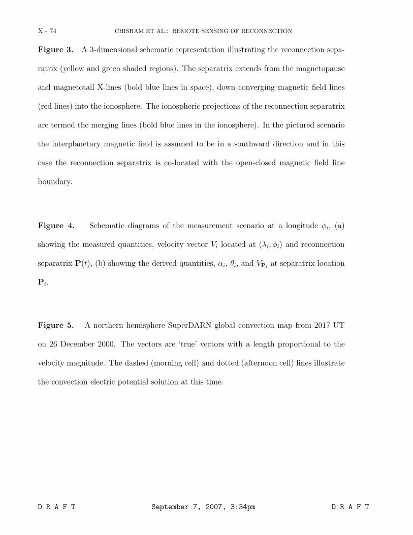
X - 74 CHISHAM ET AL.: REMOTE SENSING OF RECONNECTION
Figure 3. A 3-dimensional schematic representation illustrating the reconnection sepa-
ratrix (yellow and green shaded regions). The separatrix extends from the magnetopause
and magnetotail X-lines (bold blue lines in space), down converging magnetic field lines
(red lines) into the ionosphere. The ionospheric projections of the reconnection separatrix
are termed the merging lines (bold blue lines in the ionosphere). In the pictured scenario
the interplanetary magnetic field is assumed to be in a southward direction and in this
case the reconnection separatrix is co-located with the open-closed magnetic field line
boundary.
Figure 4. Schematic diagrams of the measurement scenario at a longitude φi, (a)
showing the measured quantities, velocity vector Vi located at (λi, φi) and reconnection
separatrix P(t), (b) showing the derived quantities, αi, θi, and VPiat separatrix location
Pi.
Figure 5. A northern hemisphere SuperDARN global convection map from 2017 UT
on 26 December 2000. The vectors are ‘true’ vectors with a length proportional to the
velocity magnitude. The dashed (morning cell) and dotted (afternoon cell) lines illustrate
the convection electric potential solution at this time.
D R A F T September 7, 2007, 3:34pm D R A F T
CHISHAM ET AL.: REMOTE SENSING OF RECONNECTION X - 75
Figure 6. A Polar UVI image of the northern hemisphere auroral oval measured at
2017:34 UT on 26 December 2000. The black symbols represent the poleward edge of the
auroral oval as estimated using the method of Carbary et al. [2003]. The red symbols
represent these estimates corrected to provide the best estimates for the OCB using the
corrections of Carbary et al. [2003]. The radial blue lines highlight the MLT sectors for
which latitudinal auroral intensity profiles are presented in fig.7.
Figure 7. Latitudinal auroral intensity profiles (solid histograms), taken from the Polar
UVI auroral image presented in fig.6 in three MLT sectors. The dotted lines illustrate the
Carbary et al. [2003] fits to the latitudinal profiles and the vertical dashed line highlights
the poleward edge as determined using the Carbary et al. [2003] algorithm.
Figure 8. The Doppler spectral width measured by beams 7-14 of the Kapuskasing
SuperDARN radar at 2017 UT on 26 December 2000. (a) The raw spectral width data, (b)
the spatially and temporally median-filtered spectral width data, and (c) the proportion of
the filtered data set that was >150 m/s (black). The dashed line represents the 1500 MLT
meridian. The white squares in (c) highlight the locations of spectral width boundaries
that were determined in this data.
D R A F T September 7, 2007, 3:34pm D R A F T

X - 76 CHISHAM ET AL.: REMOTE SENSING OF RECONNECTION
Figure 9. An example of using a truncated Fourier series to describe the OCB (at 2017-
2018 UT on 26 December 2000). The squares represent UVI boundary measurements
made between 2016 and 2019 UT and the diamonds represent SWBs measured by the
Kapuskasing, Kodiak, and Prince George SuperDARN radars during the same interval.
The solid (dotted) line represents a 10th (6th) order Fourier series.
Figure 10. (a) The distribution of Polar UVI boundary velocity in the 2000-2200
UT interval on 26 December 2000 determined from temporally adjacent samples (solid
line), at a temporal spacing of 2 samples (dashed line), and at a temporal spacing of 4
samples (dotted line). (b) The distribution of Polar UVI boundary velocity for the same
interval determined from the temporally-filtered UVI observations (solid line), and the
distributions of boundary velocity for the 6th order (dashed line) and 10th order (dotted
line) Fourier series representations of the OCB.
Figure 11. A time series of polar plots showing the development of the OCB and the
polar cap over the interval 2000-2200 UT on 26 December 2000. Each frame shows the
fitted OCB (bold line) and the raw Polar UVI and SWB boundaries used to determine
the OCB (squares). The frames represent a 1-min interval separated every 10 min.
Figure 12. A combination of the convection map presented in fig.5 with the OCB
estimate presented in fig.9 (bold line). The grey shaded regions highlight velocity vectors
located close to the OCB that are used to determine the reconnection rate.
D R A F T September 7, 2007, 3:34pm D R A F T

CHISHAM ET AL.: REMOTE SENSING OF RECONNECTION X - 77
Figure 13. The spatial variation of the reconnection rate (with MLT). (a) The variation
of the total reconnection rate. The bold black line and grey shaded region represent the
variation of the mean and standard deviation of the reconnection rate measurements de-
termined in a 2-hour MLT sliding window. (b) The contribution to the total reconnection
rate that comes from measurements of the plasma flow. (c) The contribution to the total
reconnection rate that comes from the boundary motion.
Figure 14. (a) The temporal variation in IMF By (bold line) and IMF Bz (solid line)
as measured by the ACE spacecraft, shifted by 63 min to account for the solar wind
propagation from ACE. (b) The IMF clock angle measured by ACE, shifted by 63 min
to account for the solar wind propagation from ACE. (c) The polar cap area variation
estimated from the global OCB determinations. (d) The average dayside reconnection
rate (black line). The white line represents the mean measurement determined in a 15-
min sliding window. (e) The average nightside reconnection rate (black line). The white
line represents the mean measurement determined in a 15-min sliding window. The two
vertical dashed lines represent the estimated times of a substorm onset and a substorm
intensification.
D R A F T September 7, 2007, 3:34pm D R A F T

X - 78 CHISHAM ET AL.: REMOTE SENSING OF RECONNECTION
Figure 15. A comparison of the measured variation in polar cap area (solid line)
with that predicted by the measured reconnection rate variations (dashed line), assuming
certain dayside and nightside merging line lengths. (a) Assuming fixed merging line
lengths for the whole 2-hour interval. (b) Assuming different merging line lengths in
three different time periods within the interval. The assumed merging line lengths for the
dayside and nightside are displayed on the figure as Ld and Ln respectively.
D R A F T September 7, 2007, 3:34pm D R A F T
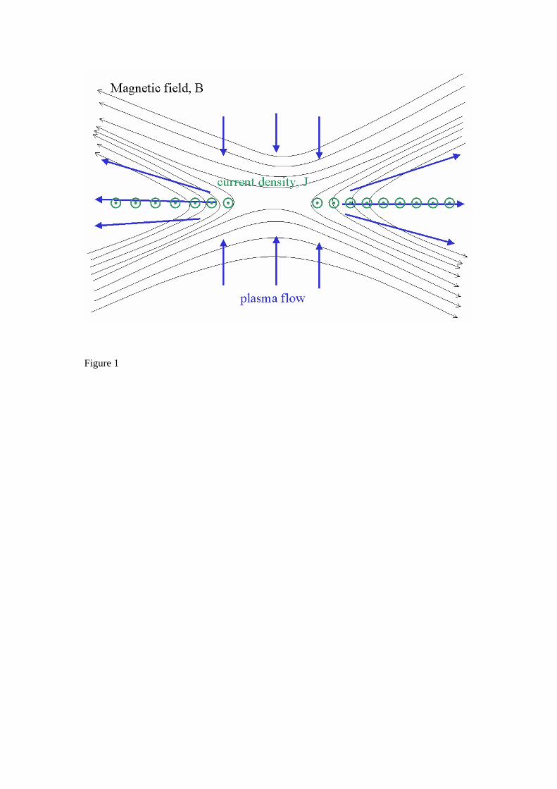
Figure 1

Figure 2

Figure 3

Figure 4a
Figure 4b

Figure 5

Figure 6

Figure 7
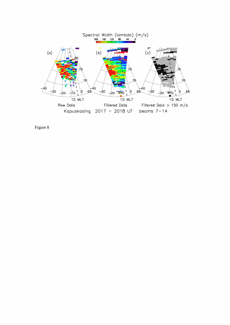
Figure 8

Figure 9

Figure 10
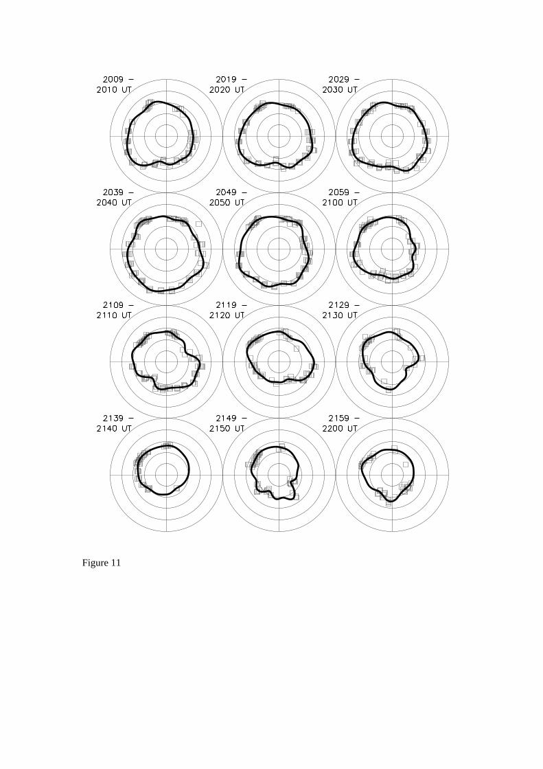
Figure 11

Figure 12
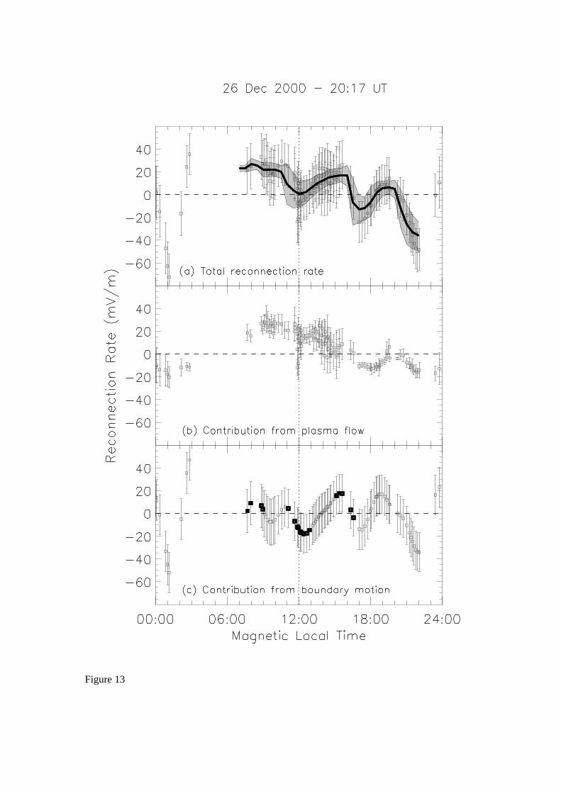
Figure 13
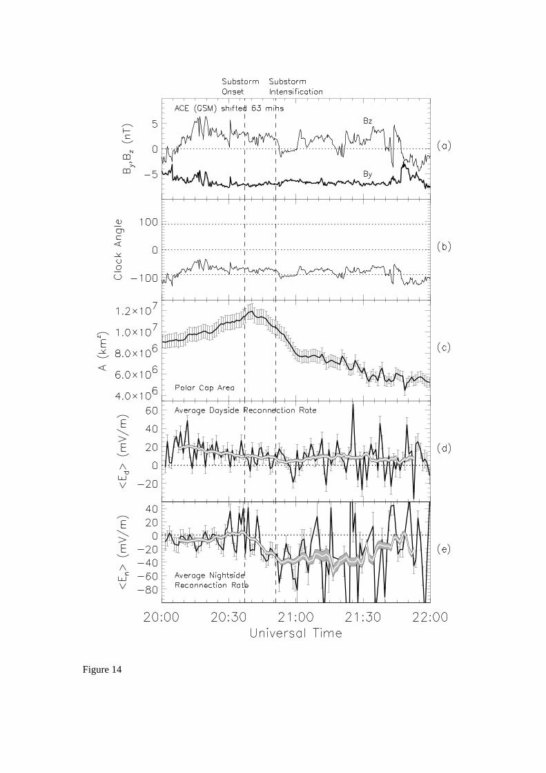
Figure 14
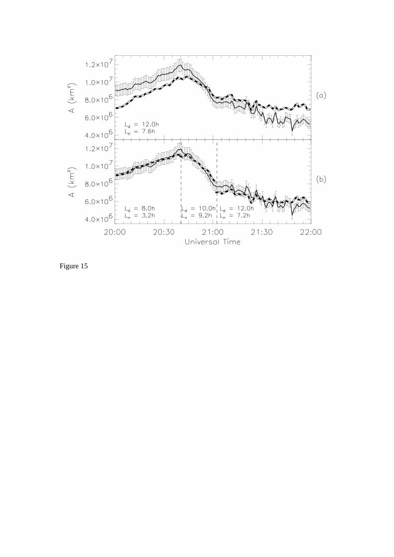
Figure 15