Relating flow channelling to tracer dispersion in heterogeneous networks

Advances in Water Resources 27 (2004) 843–855

www.elsevier.com/locate/advwatres

Relating flow channelling to tracer dispersion inheterogeneous networks

C�eline Bruderer-Weng a,*, Patience Cowie a, Yves Bernab�e b, Ian Main a

a Department of Geophysics and Geology, The University of Edinburgh, Grant Institute, West Mains Road, Edinburgh EH3 9JW, UKb Institut de Physique du Globe, 4, rue Ren�e Descartes, 67084 Strasbourg Cedex, France

Received 18 September 2002; received in revised form 7 August 2003; accepted 22 April 2004

Available online 20 July 2004

Abstract

Flow channelling is a well-documented phenomenon in heterogeneous porous media and is widely recognised to have a sub-

stantial effect on solute transport. The goal of this study is to quantify flow channelling in heterogeneous, two-dimensional, pipe

networks and to investigate its relation with dispersion. We explored the effect of pore size heterogeneity and correlation length by,

respectively, varying the normalised standard deviation of the pipe diameter distribution and imposing an exponential variogram to

their spatial distribution. By solving the flow equations, we obtained a complete description of the volumetric flow and pressure

gradient fields in each network realisation. Both fields displayed lineations but their preferential directions were roughly perpen-

dicular to each other. We estimated their multifractal dimension spectra and showed that the correlation dimension was a reliable

quantitative indicator of flow channelling. We then simulated solute dispersion in these networks using a previously published

method. We observed that flow channelling corresponded to an increase of the asymptotic dispersion coefficient and a lengthening of

the pre-asymptotic period. We conclude at the existence of a strong, but not exactly one-to-one, relation between the asymptotic

longitudinal dispersion coefficients and the correlation dimension of the flow field.

� 2004 Elsevier Ltd. All rights reserved.

Keywords: Heterogeneous media; Flow channelling; Network modelling; Contaminant transport; Dispersion; Spatial correlation; Multifractal

analysis

1. Introduction

Several recent studies have emphasised the important

role of flow channelling in groundwater flow as well as

in reservoir engineering (see [41] and references therein).

Flow channelling is associated with strong structural

heterogeneity [27,28]. It is observed at all scales, from

centimetre- to kilometre-scales and was also found toarise in numerical simulations [12,26,27]. However, a

standard method to quantify flow channelling is still

lacking. Some authors used an oversimplified approach

by imposing ‘‘structural channelling’’, i.e., by assuming

that flow may only occur in a relatively small number of

distinct, arbitrarily located, parallel channels, sometimes

*Corresponding author. Present address: Hydrosciences, ISTEEM,

UM2, Place Eug�ene Bataillon, Case MSE, 34095 Montpellier Cedex

05, France.

E-mail address: [email protected] (C. Bru-

derer-Weng).

0309-1708/$ - see front matter � 2004 Elsevier Ltd. All rights reserved.

doi:10.1016/j.advwatres.2004.05.001

incorporating tortuosity. In doing so, they were able to

model specific features of breakthrough curves such as

multiple-peaks [33,42]. De Dreuzy and co-authors [18]

developed a simple flow channelling index, applicable to

two-dimensional networks of fractures. They considered

the cross-section intersecting the smallest number of

fractures, identified the channel conducting the largest

flow qmax through this section, and quantified flowchannelling by the ratio of qmax to the remaining flow

through the same section. Our first goal in this paper is

to show that flow channelling can be quantitatively

characterised using multifractal analysis. The general-

ised dimensions are more general than an ad hoc index

as described above, and the mechanisms generating

multifractality (i.e., multiplicative cascades [17]) may

be discussed, giving an insight into the origin of chan-nelling.

Moreover, flow channelling is widely recognised to

have a large effect on dispersion [5,23,27]. It is often

blamed for the occurrence of so-called ‘‘anomalous’’

mail to: [email protected]

844 C. Bruderer-Weng et al. / Advances in Water Resources 27 (2004) 843–855

dispersion [4]. Our second objective in this work is to

investigate the effect of flow channelling on dispersion in

a conceptual porous medium, namely, two-dimensional,

heterogeneous, spatially correlated, pipe networks, thus

allowing complete determination of all relevant para-meters and variables. For this purpose, we used a pre-

viously tested method for simulating dispersion in

networks [13], estimated the values of the asymptotic

dispersion coefficient as a function of heterogeneity and

correlation length, and related it to our flow channelling

indicator, i.e., the multifractal correlation dimension D2.

The paper is organised as follows: the numerical

simulation methods are described in Section 2. Quanti-fication of flow channelling using multifractal analysis is

explained in Section 3. Section 4 presents the results of

the dispersion simulations. A concluding discussion is

given in Section 5.

Fig. 1. Examples of realisations of the pore diameter field for Nstd ¼ 1

and LC ¼ 0, 9, 21 and 42. Small values are indicated in blue and large

ones in red. (For interpretation of the references in colour in this figure

legend, the reader is referred to the web version of this article.)

2. Numerical simulation methods

Our goal was to simulate the motion of a large

number of solute particles inside the pore space of

idealised heterogeneous porous media (i.e., two-dimen-

sional networks of pipes) and quantify the time evolu-

tion of their spatial distribution. We limited our study tothe steady-state flow case. We also assumed that the

solute was conservative and chemically neutral, and that

the transport process was not affected by changes of

concentration (i.e., the individual solute particles were

treated independently). The method consisted of the

following steps:

(1) Construction of heterogeneous pipe network realisa-

tions.(2) Solution of the steady-state flow equations.

(3) Injection of the solute particles (here, a pulse at time

t ¼ 0 on a line perpendicular to the nominal flow

direction).

(4) Determination of the advective motion of each par-

ticle during the current time increment.

(5) Simulation of the diffusive motion (note that steps

(4) and (5) were performed sequentially for eachtime increment).

(6) Recording and statistical analysis of the spatial dis-

tribution of the solute particles at different times

during the transport process.

These steps will be briefly described in the next sec-

tions (see [13] for further details).

2.1. Constructing heterogeneous networks

We considered two-dimensional 100 · 100 square

networks with a constant pipe length L ¼ 400 lm. The

networks were obliquely oriented at 45� to the macro-

scopically applied pressure gradient so that the pipes

were all identically oriented with respect to the mean

flow. To facilitate determination of advective motion we

used pipes with square cross-sections [13]. Heterogeneity

was generated by randomly assigning values of the localpore ‘‘diameter’’ ai (i.e., the side length of the cross-

section of pipe i) according to log-normal distributions

with the same mean hai (i.e., 20 lm). Log-normal pore

diameter distributions are often observed in rocks [21].

In order to vary the degree of heterogeneity, we con-

sidered pore diameter distributions with different stan-

dard deviations ra. For convenience in analysing our

results, we used the normalised standard deviationra=hai, hereafter denoted Nstd, to quantify pore dia-

meter heterogeneity.

Isotropically correlated ai-fields were generated using

the turning band method (see [24] and references

therein). They were constructed with variograms fitting

an exponential model cðhÞ ¼ r2a½1� expð�3h=LC�, where

h is the separation and LC the correlation length (both

expressed in pore-length units). Examples correspondingto LC ¼ 0, 9, 21, and 42, are shown in Fig. 1, revealing

isotropically distributed high and low porosity patches.

The size of these patches was in order of magnitude

agreement with the assigned values of LC, and the iso-

tropic character was confirmed by calculations of the

corresponding permeability tensor, which was always

found to have nearly equal diagonal components and

negligible non-diagonal ones. Finally, notice that, in

C. Bruderer-Weng et al. / Advances in Water Resources 27 (2004) 843–855 845

network simulations, LC is not a continuous variable but

only takes integer values when measured in pore-length

units. Here, six different correlation lengths were used,

namely LC ¼ 0, 3, 6, 9, 21 and 42 pore lengths.

2.2. Solving the flow equations

Solving steady-state flow equations in regular net-

works has been extensively described in the literature[2,8,16]. One specific feature of the present work was

that we used pipes with square cross-section, which re-

quired a modified Poiseuille’s law:

qi ¼ �Ca4ig

DpiL

; ð1Þ

where g is the fluid viscosity, Dpi the pressure differencebetween the two nodes connected by pipe i, qi the vol-

umetric flow through it, and C was demonstrated [13] to

be equal to 0.562308. Expressing mass conservation at

each node (i.e., writing Kirchhoff’s equations) then

yields a system of linear equations whose unknowns are

the values of the fluid pressure at each node. The exact

form of the matrix depends on lattice topology and the

right-hand side vector results from the specific boundaryconditions used.

Simulating dispersion necessitates a digital represen-

tation of a very large porous body but the present

computer capabilities limit the network size. One solu-

tion is to use periodic boundary conditions for solving

the flow equations and then perform solute particle

tracking in a nominally infinite periodic array of iden-

tical networks [13]. In the case of networks with non-zero LC, large jumps in pore diameter must therefore

occur along the seams of such a network array, therefore

damaging the correlation structure. We avoided this

problem by replacing the elementary 100 · 100 network

by a combination of the original network and its mirror

images as illustrated below in the case of a 2 · 2 matrix

giving a 4 · 4 compound matrix.

a bc d

)

a b b ac d d cc d d ca b b a

Note that, in order to maximise precision, we solved the

flow equations on the compound 200 · 200 network. Thecalculated flow fields did verify the symmetries described

above within the numerical precision of the conjugate

gradient matrix solver.

The effect of pore diameter heterogeneity (i.e., Nstd)and spatial correlation (i.e., LC) on the flow pattern is

illustrated in Fig. 2 showing maps of the local volu-

metric flow qi, the mean fluid velocity in each pipe vi,and the local pressure gradient Dpi=L in various reali-

sations of the elementary network. Fig. 2a displays three

examples of moderately heterogeneous networks (i.e.,

Nstd ¼ 0:4), with LC increasing from 0 to 42, whereas

Fig. 2b corresponds to the strong heterogeneity case

(i.e., Nstd ¼ 1:0). It appears clearly that flow channelling

increases with increasing Nstd and LC. Notice also that

the qi- and Dpi-fields are very similar to each other, withvisually identical degrees of localisation (i.e., channelling

in the case of the flow field). The only difference is that

the preferential flow paths are oriented sub-parallel to

the applied pressure gradient (or, equivalently, the

macroscopic flow direction) whereas the pressure gra-

dient lineations are perpendicular to it. To the contrary,

the mean velocity field (or vi-field) has a roughly iso-

tropic, patchy structure with no visible lineations. Notethat the vi-fields calculated in these networks appeared

quite similar to experimentally measured ones [32]. In

particular, we observed that the longitudinal velocity

component had an extremely asymmetric distribution

while the distribution of the transverse component was

approximately Gaussian [32]. Thus, the qi-, Dpi- and vi-fields, despite their obvious interdependence, are not

simply correlated with each other as is sometimes as-sumed [39]. Indeed, these three quantities satisfy the

following proportionality relations:

vi /qia2i

ð2aÞ

and

Dpi /qia4i

; ð2bÞ

where the pore diameter ai is a log-normal random field.

It is therefore not surprising that a high (alternatively,

low) mean velocity in any given pipe is not necessarily

associated with a large (alternatively, small) flow. For

example, high flow can occur through very wide pipes

with a low mean velocity. The same is true for flow and

pressure gradient (see [8] for spatially uncorrelated net-

works). Recent unpublished work using other two- andthree-dimensional lattices indicates that the qi- and Dpi-fields may not always be as strikingly similar to each

other as in the two-dimensional square lattice case de-

scribed above. However, the effect of lattice topology

and dimensionality is out of the scope of this article and

will not be discussed further.

2.3. Simulating dispersion

We used the same simulation method as in [13]. The

idea is to numerically track the motion inside the pore

space of a large number of independent solute particles,simultaneously subjected to advection and molecular

diffusion (i.e., the two physical mechanisms acting at the

scale of the solute particles). These two micro-mecha-

nisms are independent and additive allowing us to sim-

ulate them sequentially at each time step as will be

described in Sections 2.3.1 and 2.3.2.

Fig. 2. Illustration of the influence of Nstd and LC on the qi-, vi- and Dpi-fields, (a) for a moderate heterogeneity (i.e., Nstd ¼ 0:4), and (b) a high

heterogeneity (i.e., Nstd ¼ 1:0). In both cases, we showed realisations corresponding to LC ¼ 0, 9 and 42. In these images, each individual pipe is

represented by a very short, inclined segment, the thickness of which is proportional to qi, vi or Dpi.


This approach is quite different from other, previ-

ously published, particle-tracking/random-walk simula-

tion methods. In one type of study [25,27], the porous

medium is considered a continuum and the Darcy flow


field is calculated. A random-walk can be superposed on

the Darcy advective motion to simulate small-scale

dispersion [25] with a dispersion coefficient that depends

on the local Darcy velocity. Mass conservation prob-

lems arise in strongly heterogeneous media with sharpvariations of the permeability and, therefore, velocity

fields [25]. Here, the small-scale mixing process is

molecular diffusion, hence totally independent of

advection (note also that mass conservation is guaran-

teed in networks). Another type of study is based on

network simulation [26,37]. However, the advection and

diffusion processes are generally modelled in an over-

simplified, unphysical way. The particle motion in theconduits is purely advective and deterministic (the par-

ticle velocity in each conduit is equal to the conduit

mean velocity). The stochastic mixing process is imple-

mented exclusively at the nodes (i.e., when they reach a

node, the particles randomly choose the conduit inside

which their advective motion will continue). Clearly, this

is incompatible with Taylor-Aris dispersion in a set of

capillaries connected in series. To the contrary, ourmethod did accurately produce Taylor-Aris dispersion

in a single capillary [13]. Our method was previously

tested in heterogeneous networks with LC ¼ 0 [13], and

we observed that tracking 2000 particles produced rea-

sonably stable results. More recently, we applied it using

different network sizes between 40 · 40 and 200 · 200and found no significant size effect on dispersion. Fi-

nally, we tried different types of pore diameter distri-bution (uniform, log-uniform, normal, log-normal) and

observed only negligible differences in the dispersion

coefficients for equal heterogeneity Nstd.

2.3.1. Advection

Under advective transport, a solute particle passively

follows the fluid streamline on which it is located.Advection is therefore a deterministic process. In steady-

state flow conditions, the streamline geometry does not

vary with time. In the networks, the streamlines in each

pipe are straight lines parallel to the pipe axis. The

problem is to determine how these straight streamlines

connect to each other at the nodes of the network. This

can be done in two-dimensional networks by using mass

conservation and a rule forbidding streamlines tointersect (for further details, see [13]). Extension of this

method to three-dimensional networks requires an

additional rule, which we have not established yet. This

is the major reason why this study was restricted to two-

dimensional networks (however note that two-dimen-

sional simulations can nevertheless be relevant to

situations such as flow through a single fracture [43]).

2.3.2. Molecular diffusion

Molecular diffusion is modelled as a discrete random

walk superposed on the advective motion. At fixed time

intervals dt, a solute particle instantaneously jumps over

a fixed distance dr in a random direction from its present

location. Solute particles thus hop from one streamline

to another. The velocity change is assumed to be

instantaneous, and the advective motion resumes

immediately after the jump on the new streamline. Inaddition, we use a simple mirror reflection rule for the

particles colliding with the solid/pore interface. The

parameters dt and dr define the molecular diffusion

coefficient Dm simulated [34]:

Dm ¼ dr2=6dt: ð3ÞTo insure accuracy, dr must be smaller than ai. On

the other hand, dt cannot be chosen too small since it is

inversely proportional to the total number of jumps

performed during the simulations, itself proportional to

the total CPU time. We had to settle on values yielding a

diffusion coefficient of 4.4 · 10�14 m2/s, rather small

compared to realistic values of Dm in aqueous solutions.

The global hydrodynamic conditions can be quantifiedby the P�eclet number Pe ¼ LU=Dm, where U is Darcy’s

velocity. To reduce the number of parameters in the

present study, we kept the P�eclet number constant,

Pe ¼ 290. This value is not unrealistic in natural situa-

tions and corresponds to a Darcy’s velocity of

3.26 · 10�8 m/s.

2.4. Calculating dispersion coefficients

Fickian dispersion is characterised by a linear growth

of the second spatial moment r2L of the solute concen-

tration with time (the subscript L refers to the longitu-

dinal dispersion; transverse dispersion will not be

discussed in this paper). In that case, the dispersion

coefficient DL ¼ dr2L=dt is a constant depending on the

medium properties and structure, and on the P�ecletnumber as defined above. However, Fickian behaviour

is not instantaneously established in heterogeneous

porous media. Instead, it is generally observed that

Fickian dispersion is asymptotically approached after a

certain time s elapsed. During this transitory period (i.e.,

for t < s), DL increases with time and distance of

observation, or equivalently, the second moment in-creases at a rate that is non-linear in time, possibly in a

power-law fashion r2L / ta, with a > 1 [5,38]. Solute

transport characterised by dispersion coefficient

increasing with time and distance is usually called

‘‘anomalous’’ dispersion (or, alternatively, ‘‘non-Fic-

kian’’, ‘‘pre-asymptotic’’, or ‘‘scale-dependent’’ [4,5,10]).

Here, we considered heterogeneous networks con-

taining a unique disorder-scale LC. In such networks,solute transport does eventually become Fickian at large

times (i.e., for t > s). But, for Nstd as large as those used

here, s was comparable to the maximum time tmax that

we can presently simulate [13]. Consequently, the

asymptotic dispersion coefficient D�L could not be simply

estimated as the linear slope of 1=2r2Lt) at large times

00 t

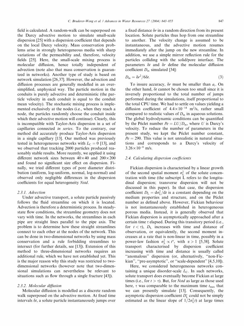
s+b = 2DL*s

0 9 21 42

LC

0

2e+10

4e+10

6e+10

8e+10

1e+11

0 5e+06 1e+07 1.5e+07 2e+07

t (s)

0 9 21 42

LC

σ L2 (

µm2)

0

2e+10

4e+10

6e+10

8e+10

1e+11

σ L2

(µm

2)

σ L2

(a)

(c)

(b)

0 5e+06 1e+07 1.5e+07 2e+07

t (s)

Fig. 3. Illustration of the time evolution of r2L: (a) a graphic repre-

sentation of Eq. (4) and the short- and long-time behaviours, (b) and

(c), examples of r2LðtÞ curves for Nstd ¼ 0:4 and 1.0, respectively. In

both cases, LC was equal to 0, 9, 21 and 42.


because the implied condition tmax � s was not always

fulfilled. Several models published in the literature pre-

dict the time-evolution of r2L in the case of a medium

containing a single disorder-scale. For example,

expressions for r2LðtÞ were derived using a first-order

perturbation expansion by Dagan [15], and Dentz and

co-authors [19,20] used a second-order perturbation

expansion to express temporal behaviour of effective and

ensemble average dispersion coefficients. In all these

models, Fickian behaviour is reached at a time s that

depends on the medium correlation length, the spatial

extension of the solute initial injection, the fluid velocity

and the small-scale dispersion tensor (notice that s maygrow indefinitely in hierarchical systems). However,

these models are based on assumptions that are poorly

satisfied in our networks (e.g., the porous medium is a

continuum, the spatial fluctuations of the hydraulic

properties of the medium are small, the correlation

length is a continuous variable).

Instead, we preferred to use a new method specifically

designed for our networks. It is based on an expressionthat smoothly connects the asymptotic linear behaviour

at large times (slope equal to 2D�L) to a generalisation of

the linear behaviour theoretically predicted for a single

capillary at very short times (slope of the tangent at

t ¼ 0, equal to 2Dm [45]):

r2LðtÞ ¼ sð þ bÞt þ bsðe�t=s � 1Þ; ð4Þ

where s is the initial slope, sþ b the asymptotic slope

and s is the transitory time-scale (see Fig. 3a). Eq. (4)

corresponds to an initial solute distribution implying

r2Lð0Þ ¼ 0 (i.e., a pulse of 2000 particles injected at t ¼ 0

in the nodes along the left edge of one 200 · 200 com-

pound network). Notice that Eq. (4) did agree satisfac-torily with Dagan’s model [15] using similar values for

the shared parameters and adjusting the additional ones

in a reasonable way.

Thus, our problem was to find the best fitting

parameters s, b and s for each network realisation. It

turns out that s was always orders of magnitude smaller

than b and, therefore, very poorly resolved by the non-

linear fitting method used here (the Levenberg–Marqu-ardt iterative algorithm [31]). As a consequence, we

decided to set s to its theoretical value s ¼ 2Dm and only

determine b and s. Several examples are presented on

Fig. 3b and c for Nstd ¼ 0:4 and 1.0, respectively.

Visually, the fitting quality is very good. As the exam-

ples of Fig. 3b and c show, the asymptotic dispersion

coefficient D�L ¼ ðsþ bÞ=2 tended to increase with LC

and Nstd. Note that the non-linearity of the r2LðtÞ curve

was always apparent (except maybe for LC ¼ 0). In

order to help assessing the orders of magnitude obtained

here, we report measured values of D�L of 10�11–10�10

m2/s and s ranging from 5 · 105 to 107 s for LC ¼ 0 and

Nstd ¼ 0:2 and 0.6, respectively. Finally, we should

point out that this analysis was performed on 100 dif-

ferent network realisations for each pair of values of LC

and Nstd examined here, and that ensemble averages will

be reported in Section 4. Notice also that the transitory

behaviour is out of the scope of this article and, in

particular, s will not be discussed in details in the fol-lowing sections.

3. Quantification of flow channelling

It is now widely recognised that flow channelling

occurs in aquifers at all scales, from centimetre- to

kilometre-scale, and strongly affects solute transport

[1,41,42,44]. Here, our goal is to document the causal

sequence, in pipe networks, from pore diameter heter-

-7

-6

-5

-4

-3

-2

-1

0

-1.8 -1.6 -1.4 -1.2 -1 -0.8 -0.6 -0.4 -0.2 0

log(ε)

q=0

q=-4

q=4

-4 3.682-3 3.471-2 3.141-1 2.6140 21 1.6712 1.5503 1.4884 1.448

q Dq

log(

Mq

1/(

1-q

) )

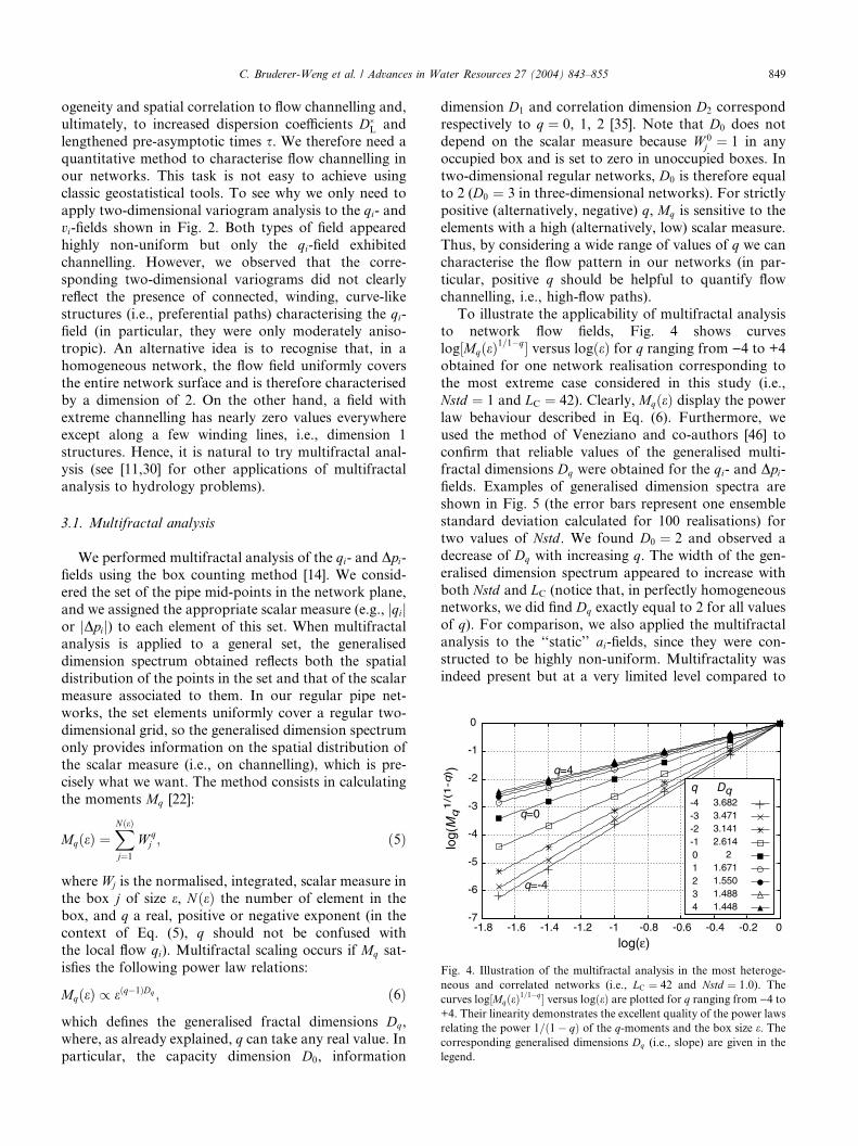
Fig. 4. Illustration of the multifractal analysis in the most heteroge-

neous and correlated networks (i.e., LC ¼ 42 and Nstd ¼ 1:0). The

curves log½MqðeÞ1=1�q� versus logðeÞ are plotted for q ranging from )4 to+4. Their linearity demonstrates the excellent quality of the power laws

relating the power 1=ð1� qÞ of the q-moments and the box size e. Thecorresponding generalised dimensions Dq (i.e., slope) are given in the

legend.


ogeneity and spatial correlation to flow channelling and,

ultimately, to increased dispersion coefficients D�L and

lengthened pre-asymptotic times s. We therefore need a

quantitative method to characterise flow channelling in

our networks. This task is not easy to achieve usingclassic geostatistical tools. To see why we only need to

apply two-dimensional variogram analysis to the qi- andvi-fields shown in Fig. 2. Both types of field appeared

highly non-uniform but only the qi-field exhibited

channelling. However, we observed that the corre-

sponding two-dimensional variograms did not clearly

reflect the presence of connected, winding, curve-like

structures (i.e., preferential paths) characterising the qi-field (in particular, they were only moderately aniso-

tropic). An alternative idea is to recognise that, in a

homogeneous network, the flow field uniformly covers

the entire network surface and is therefore characterised

by a dimension of 2. On the other hand, a field with

extreme channelling has nearly zero values everywhere

except along a few winding lines, i.e., dimension 1

structures. Hence, it is natural to try multifractal anal-ysis (see [11,30] for other applications of multifractal

analysis to hydrology problems).

3.1. Multifractal analysis

We performed multifractal analysis of the qi- and Dpi-fields using the box counting method [14]. We consid-

ered the set of the pipe mid-points in the network plane,

and we assigned the appropriate scalar measure (e.g., jqijor jDpij) to each element of this set. When multifractal

analysis is applied to a general set, the generalised

dimension spectrum obtained reflects both the spatial

distribution of the points in the set and that of the scalar

measure associated to them. In our regular pipe net-

works, the set elements uniformly cover a regular two-

dimensional grid, so the generalised dimension spectrum

only provides information on the spatial distribution ofthe scalar measure (i.e., on channelling), which is pre-

cisely what we want. The method consists in calculating

the moments Mq [22]:

MqðeÞ ¼XNðeÞ

j¼1

W qj ; ð5Þ

where Wj is the normalised, integrated, scalar measure in

the box j of size e, NðeÞ the number of element in the

box, and q a real, positive or negative exponent (in the

context of Eq. (5), q should not be confused with

the local flow qi). Multifractal scaling occurs if Mq sat-

isfies the following power law relations:

MqðeÞ / eðq�1ÞDq ; ð6Þ

which defines the generalised fractal dimensions Dq,

where, as already explained, q can take any real value. In

particular, the capacity dimension D0, information

dimension D1 and correlation dimension D2 correspond

respectively to q ¼ 0, 1, 2 [35]. Note that D0 does not

depend on the scalar measure because W 0j ¼ 1 in any

occupied box and is set to zero in unoccupied boxes. In

two-dimensional regular networks, D0 is therefore equalto 2 (D0 ¼ 3 in three-dimensional networks). For strictly

positive (alternatively, negative) q, Mq is sensitive to the

elements with a high (alternatively, low) scalar measure.

Thus, by considering a wide range of values of q we can

characterise the flow pattern in our networks (in par-

ticular, positive q should be helpful to quantify flow

channelling, i.e., high-flow paths).

To illustrate the applicability of multifractal analysisto network flow fields, Fig. 4 shows curves

log½MqðeÞ1=1�q� versus logðeÞ for q ranging from )4 to +4

obtained for one network realisation corresponding to

the most extreme case considered in this study (i.e.,

Nstd ¼ 1 and LC ¼ 42). Clearly, MqðeÞ display the power

law behaviour described in Eq. (6). Furthermore, we

used the method of Veneziano and co-authors [46] to

confirm that reliable values of the generalised multi-fractal dimensions Dq were obtained for the qi- and Dpi-fields. Examples of generalised dimension spectra are

shown in Fig. 5 (the error bars represent one ensemble

standard deviation calculated for 100 realisations) for

two values of Nstd. We found D0 ¼ 2 and observed a

decrease of Dq with increasing q. The width of the gen-

eralised dimension spectrum appeared to increase with

both Nstd and LC (notice that, in perfectly homogeneousnetworks, we did find Dq exactly equal to 2 for all values

of q). For comparison, we also applied the multifractal

analysis to the ‘‘static’’ ai-fields, since they were con-

structed to be highly non-uniform. Multifractality was

indeed present but at a very limited level compared to

0.8

1

1.70

1.65D2

-4 -3 -2 -1 0 1 2 3 41

1.5

2

2.5

3

3.5

4

q

Dq

Nstd=0.4

-4 -3 -2 -1 0 1 2 3 41

1.5

2

2.5

3

3.5

4

q

Nstd=1.0

Dq

0 9 21 42

LC

0 9 21 42

LC

(a)

(b)

Fig. 5. Examples of generalised dimension spectra for (a) Nstd ¼ 0:4 and (b) Nstd ¼ 1:0 (with LC ¼ 0, 9, 21 and 42).


the qi- and Dpi-fields (e.g., the minimum value of D2 was

1.92 for the ai-field whereas 1.55 was measured for theqi- and Dpi-fields).

0 10 20 30 400

0.2

0.4

0.6

Nst

d

1.951.90

1.80

1.971.99

LC

Fig. 6. A contour plot of the correlation dimension D2 of the qi-fieldversus the structural parameters LC and Nstd.

3.2. Relating D2 and flow channelling

Since the variations of a single generalised dimensionare much easier to quantify than the evolution of the

entire multifractal spectrum, we simplified the procedure

for all other values of Nstd and LC examined here, and

only determined the correlation dimension D2 of the qi-field. This choice of q ¼ 2 appeared logical since our

ultimate goal was to establish a relation with the dis-

persion coefficient. Additional justifications were that a

positive q was required for characterising the high-flowsub-set, and q ¼ 2 seemed to be a good compromise

between a small range of variation for small q and large

uncertainties for increasing q. The variations of D2 as a

function of Nstd and LC are summarised in Fig. 6. We

found that D2 was equal to the network topological

dimensional (i.e., 2) in homogeneous networks, and

gradually decreased with increasing LC and/or Nstd. Theminimum value reached here was 1.55 (for Nstd ¼ 1 andLC ¼ 42). Visual inspection of the corresponding qi-fields suggests that decreasing D2 corresponded to

increasing flow channelling. We speculate that Dþ1should approach 1 when the set of high-flow points is

reduced to a single channel, resulting in a significant

decrease of D2 as well. On the other hand, D�1 is not

necessarily limited by 2, as would be the case if the low-

flow points had identical, near-zero values of qi. Indeed,a simple inspection of the 1=qi-fields shows that their

variance keeps increasing as the conditions of maximum

channelling are approached. In order to confirm our

interpretation of D2 as a channelling indicator, we fol-

lowed De Dreuzy et al.’s idea [18] and defined a chan-

nelling index CDr ¼ qmax=hqi. In our networks, CDr

varies between 1/200 in a homogeneous 100 · 100 net-

work (i.e., no channelling) to unity in a network with aflow field reduced to a single channel (i.e., maximum

channelling). Fig. 7 shows that, in our networks, D2 and

CDr were strongly related to each other, confirming that

D2 is a good channelling indicator. It is clear also that D2

and CDr were not linked by an exactly one-to-one rela-

tion, but this is a secondary point that will not be dis-

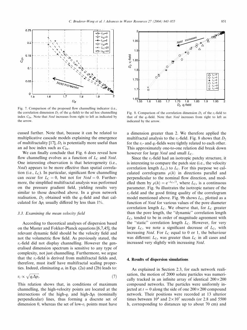
Fig. 7. Comparison of the proposed flow channelling indicator (i.e.,

the correlation dimension D2 of the qi-field) to the ad hoc channelling

index CDr. Note that Nstd increases from right to left as indicated by

the arrow.

1.55 1.6 1.65 1.7 1.75 1.8 1.85 1.9 1.95 21.65

1.7

1.75

1.8

1.85

1.9

1.95

2

D2

v i-f

ield

LC =0LC =3LC =6LC =9LC =21LC =42

D2 qi-field

Nstd increases

Fig. 8. Comparison of the correlation dimension D2 of the vi-field to

that of the qi-field. Note that Nstd increases from right to left as

indicated by the arrow.


cussed further. Note that, because it can be related to

multiplicative cascade models explaining the emergence

of multifractality [17], D2 is potentially more useful than

an ad hoc index such as CDr.

We can finally conclude that Fig. 6 does reveal how

flow channelling evolves as a function of LC and Nstd.One interesting observation is that heterogeneity (i.e.,

Nstd) appears to be more effective than spatial correla-tion (i.e., LC). In particular, significant flow channelling

can occur for LC ¼ 0, but not for Nstd ¼ 0. Further-

more, the simplified multifractal analysis was performed

on the pressure gradient field, yielding results very

similar to those described above. In a given network

realisation, D2 obtained with the qi-field and that cal-

culated for Dpi usually differed by less than 1%.

3.3. Examining the mean velocity field

According to theoretical analyses of dispersion basedon the Master and Fokker-Planck equations [6,7,45], the

relevant dynamic field should be the velocity field and

not the volumetric flow field. As previously stated, the

vi-field did not display channelling. However the gen-

eralised dimension spectrum is sensitive to any type of

complexity, not just channelling. Furthermore, we argue

that the vi-field is derived from multifractal fields and,

therefore, must itself have multifractal scaling proper-ties. Indeed, eliminating ai in Eqs. (2a) and (2b) leads to:

vi /ffiffiffiffiffiffiffiffiffiffiffiqiDpi

p: ð7Þ

This relation shows that, in conditions of maximum

channelling, the high-velocity points are located at the

intersections of the high-qi and high-Dpi (nominally

perpendicular) lines, thus forming a discrete set of

dimension 0, whereas the set of low-vi points must have

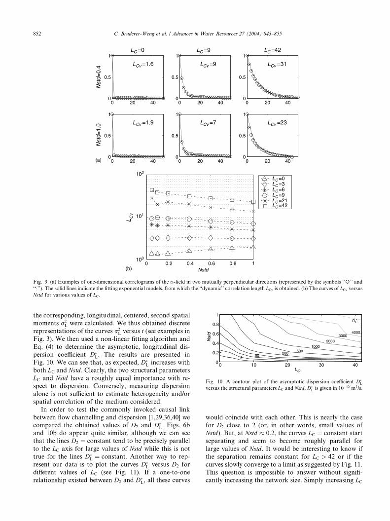
a dimension greater than 2. We therefore applied themultifractal analysis to the vi-field. Fig. 8 shows that D2

for the vi- and qi-fields were tightly related to each other.

This approximately one-to-one relation did break down

however for large Nstd and small LC.

Since the vi-field had an isotropic patchy structure, it

is interesting to compare the patch size (i.e., the velocity

correlation length LCv) to LC. For this purpose we cal-

culated correlograms qðhÞ in directions parallel andperpendicular to the nominal flow direction, and mod-

elled them by qðhÞ ¼ e�LCv=3, where LCv is a continuous

parameter. Fig. 9a illustrates the isotropic nature of the

vi-field and the good fitting quality of the correlogram

model mentioned above. Fig. 9b shows LCv plotted as a

function of Nstd for various values of the pore diameter

correlation length LC. We observe that, for LC greater

than the pore length, the ‘‘dynamic’’ correlation lengthLCv tended to be in order of magnitude agreement with

the ‘‘static’’ correlation length LC. However, for very

large LC, we note a significant decrease of LCv with

increasing Nstd. For LC equal to 0 or 1, the behaviour

was different: LCv was greater than LC in all cases and

increased very slightly with increasing Nstd.

4. Results of dispersion simulations

As explained in Section 2.3, for each network reali-

sation, the motion of 2000 solute particles was numeri-cally tracked in an infinite array of identical 200 · 200compound networks. The particles were uniformly in-

jected at t ¼ 0 along the side of one 200 · 200 compound

network. Their positions were recorded at 13 ulterior

times between 104 and 2 · 107 seconds (or 2.8 and 5500

h, corresponding to distances up to about 70 cm) and

0 20 400

0.5

1LC =0

LCv =1.6

0 20 400

0.5

1

LCv =1.9

0 20 400

0.5

1LC =9

LCv =9

0 20 400

0.5

1

LCv =7

0 20 400

0.5

1LC =42

LCv =31

0 20 400

0.5

1

LCv =23

Nst

d=0.

4N

std=

1.0

(a)

(b)0 0.2 0.4 0.6 0.8 1

100

101

102

LC =0 LC =3LC =6LC =9LC =21LC =42

Nstd

L Cv

Fig. 9. (a) Examples of one-dimensional correlograms of the vi-field in two mutually perpendicular directions (represented by the symbols ‘‘�’’ and

‘‘�’’). The solid lines indicate the fitting exponential models, from which the ‘‘dynamic’’ correlation length LCv is obtained. (b) The curves of LCv versus

Nstd for various values of LC.

DL*

0 10 20 30 400

0.2

0.4

0.6

0.8

1

Nst

d

LC

4000

5200

5001000

20003000

50

Fig. 10. A contour plot of the asymptotic dispersion coefficient D�L

versus the structural parameters LC and Nstd. D�L is given in 10�12 m2/s.


the corresponding, longitudinal, centered, second spatial

moments r2L were calculated. We thus obtained discrete

representations of the curves r2L versus t (see examples in

Fig. 3). We then used a non-linear fitting algorithm and

Eq. (4) to determine the asymptotic, longitudinal dis-

persion coefficient D�L. The results are presented in

Fig. 10. We can see that, as expected, D�L increases with

both LC and Nstd. Clearly, the two structural parameters

LC and Nstd have a roughly equal importance with re-

spect to dispersion. Conversely, measuring dispersion

alone is not sufficient to estimate heterogeneity and/or

spatial correlation of the medium considered.

In order to test the commonly invoked causal link

between flow channelling and dispersion [1,29,36,40] wecompared the obtained values of D2 and D�

L. Figs. 6b

and 10b do appear quite similar, although we can see

that the lines D2 ¼ constant tend to be precisely parallel

to the LC axis for large values of Nstd while this is not

true for the lines D�L ¼ constant. Another way to rep-

resent our data is to plot the curves D�L versus D2 for

different values of LC (see Fig. 11). If a one-to-one

relationship existed between D2 and D�L, all these curves

would coincide with each other. This is nearly the case

for D2 close to 2 (or, in other words, small values of

Nstd). But, at Nstd � 0:2, the curves LC ¼ constant start

separating and seem to become roughly parallel for

large values of Nstd. It would be interesting to know if

the separation remains constant for LC > 42 or if the

curves slowly converge to a limit as suggested by Fig. 11.

This question is impossible to answer without signifi-cantly increasing the network size. Simply increasing LC

1.65 1.7 1.75 1.8 1.85 1.9 1.95 210-1

100

101

102

103

104

D2

DL*

LC =0

LC =3

LC =6 LC =9 LC =21

LC =42

Nstd increases

Fig. 11. A summary of the relationship between D�L and the correla-

tion dimension D2 of the qi-field. In this representation, the data are

grouped to form LC ¼ constant lines (with LC ¼ 0, 3, 6, 9, 21 and 42).

As indicated by the arrow, Nstd increases from right to left along each

line.


is not a solution since important statistical assumptions

such as ergodicity, become invalid for LC comparable

to the network size (in fact, LC ¼ 42 might already

be above this limit). Finally, note that, for Nstdapproaching zero, the curves LC ¼ constant continu-

ously converge towards a single point (D2 ¼ 2; D�L ¼

Dhom), where Dhom ¼ 7� 10�13 m2/s is the dispersion

coefficient of a perfectly homogeneous network.

5. Discussion and conclusions

The results reported above support four main con-

clusions:

1. In statistically isotropic, heterogeneous pipe net-

works, flow channelling intensifies when Nstd and/or

LC are increased.2. The three ‘‘dynamic’’ fields characterising steady-

state fluid flow in the networks (namely, the qi-, vi-and Dpi-fields) have multifractal scaling properties,

which vary with Nstd and/or LC.

3. The correlation dimension D2 of the qi-field can be

used as a quantitative indicator of flow channelling.

4. Dispersion is strongly affected by flow channelling. In

other words, the asymptotic dispersion coefficient D�L

and the correlation dimension D2 of the qi-field are

tightly linked to each other, although an exact one-

to-one relationship did not hold.

Our results, as expressed in conclusion (1), agree with

previous findings in field [1,41], laboratory [30,36], and

continuum simulations [12,27] studies. Note also that we

obtained qi- and vi-fields qualitatively similar to those

observed in laboratory experiments [32] and fracture

network simulations [26]. The relation of these ‘‘dy-

namic’’ fields to each other and to the underlying,

‘‘static’’, pore diameter ai-field was found to be rathercomplex. The qi- and Dpi-fields always exhibited linea-

tions (oriented at 90� to each other) whereas the

underlying pore structure was constructed statistically

isotropic and did not include structural lineations.

Moreover, we observed that the corresponding vi-fieldsdid not display channelling but had an isotropic patchy

structure, suggesting that, for a large part, flow chan-

nelling results from conservation of mass. We measureda non-zero ‘‘dynamic’’ correlation length LCv in all cases,

even when the ‘‘static’’ correlation length LC was zero.

On the other hand, for LC greater than 1 or 2 pore

lengths, LCv was found to be smaller than LC, sometimes

by as much as a factor of 2. A second conclusion was

that the qi- and Dpi-fields are much more multifractal

than the underlying ai-fields, and become more so with

increasing LC and Nstd. We think that some of the fea-tures described here are sufficiently general to remain

valid in physical porous media or in continuum simu-

lations. In particular, the multifractality of the ‘‘dy-

namic’’ fields could be very useful to interpret the

results of field, laboratory of numerical simulation

experiments.

As stated in conclusions (3) and (4), we determined

the variations of the correlation dimension D2 of the qi-field as a function of LC and Nstd, and demonstrated

that it had a substantial relationship to flow channelling

and, ultimately, to dispersion. However it is clear that,

although strongly related, the correlation dimension D2

of the qi-field and D�L were not linked by an exact one-to-

one relation. One reasonable explanation is that dis-

persion is not solely governed by flow channelling. Yet,

this explanation is not fully satisfactory because theapproximate D2 $ D�

L relation broke down at relatively

small values of Nstd (i.e., at low levels of flow channel-

ling) and the separation did not increase afterwards (see

Fig. 11). Alternatively, it may be that the generalised

dimension spectra do not provide the most adequate

way to quantify flow channelling, or cannot be fully

characterised by a single parameter such as D2.

We also saw that, according to theoretical analyses ofdispersion based on the Master and Fokker-Planck

equations [6,7,45], the relevant dynamic field should be

the velocity field and not the volumetric flow field. But

we observed that the relation between D�L and D2 was

not improved by using the vi- instead of the qi-field.Nevertheless, the vi-field is an important ‘‘dynamic’’

field. In pipe networks, it is linked to the other ‘‘dy-

namic’’ fields through Eq. (7). Hence, the question arisesto find the equivalent of Eq. (7) in porous continua. Eqs.

(2a) and (2b) must be replaced by Darcy’s law and

Dupuit-Forcheimer’s equation:


qi / kiDpi ð8aÞ

and

vi /qi/i

; ð8bÞ

where ki is the local permeability and /i the local

porosity. There is no ‘‘universal’’ permeability–porosity

relationship valid for all porous media but power lawrelations, ki / /a

i , have been found to apply in specific

situations. In principle, the exponent a ranges between

zero and infinity (note that a < 1 are essentially never

observed; see [9] for a more complete discussion). Using

the above power law allows elimination of ki and /i

from Eqs. (8a) and (8b), leading to:

vi / q1�1=ai Dp1=ai : ð9Þ

In the extreme case corresponding to very large a, thevelocity field is simply proportional to the volumetric

flow (i.e., discharge) field. In the other extreme case,

a ¼ 1, the velocity field is proportional to the pressure

gradient field. In sub-surface hydrological systems,

porosity (unlike permeability) has a rather limited range

of variation, implying that a must take large values. Forexample, consider the case of clean sand, the properties

of which are controlled by mean grain size and sorting

[3]. If, in a given location, only grain size varies, porosity

is constant and the exponent a must diverge to infinity,

leading to vi / qi. If sorting changes while the mean

grain size remains constant, experimental data from [3]

produce values of a on the order of 10, still approxi-

mately yielding vi / qi. Small values of a (i.e., from 1 to3) are expected in systems with a wide range of variation

of porosity and very slowly evolving pore connectivity

and/or small-scale heterogeneity [9]. In consequence,

small values of a should not be relevant to problem

concerning fractured reservoirs or the vadose zone, in

which pore connectivity and small-scale heterogeneity

can display very sharp spatial variations. We can

therefore conclude that vi / qi in most hydrologicalsystems. Channelling similar to that observed in the

network qi-fields, should thus be present in measured or

simulated large-scale vi-fields, and multifractal analysis

should be a helpful characterisation tool.

Acknowledgements

The critical but sagacious and insightful comments of

D.A. Barry, L. Moreno, M. Dentz and an anonymousreviewer helped us improve this paper. We are very

grateful to Rebecca Lunn for kindly giving access to her

turning band code for generating spatial correlation. CB

was funded by EU grants CT97-0456 (DG12)-‘‘SCAL-

FRAC’’, and EVK1-CT-2000-00062-‘‘SALTRANS’’.

References

[1] Abelin H, Birgersson L, Gidlund J, Neretnieks I. A large scale

flow and tracer experiment in granite: 1. Experimental design and

flow distribution. Water Resour Res 1991;27:3107–17.

[2] Adler PM. Porous media: geometry and transport. Boston, MA:

Butter-Heinemenn; 1992.

[3] Beard DC, Weyl PK. Influence of texture on porosity and

permeability of unconsolidated sand. Am Assoc Pet Geol Bull

1973;57:349–69.

[4] Berkowitz B. Dispersion in heterogeneous geological formations.

London: Kluwer Academic Publishers; 2001.

[5] Berkowitz B. Characterizing flow and transport in fractured

geological media: a review. Adv Water Resour 2002;25:861–84.

[6] Berkowitz B, Klafter J, Metzler R, Scher H. Physical pictures of

transport in heterogeneous media: advection-dispersion, random-

walk, and fractional derivative formulations. Water Resour Res

2002;38:1191, doi:10.1029/2001WR001030.

[7] Berkowitz B, Scher H. Anomalous transport in random fracture

networks. Phys Rev Lett 1997;79:4038–41.

[8] Bernab�e Y, Bruderer C. Effect of the variance of the pore size

distribution on the transport properties of heterogeneous net-

works. J Geophys Res 1998;103:513–25.

[9] Bernab�e Y, Mok U, Evans B. Permeability–porosity relationships

in rocks subjected to various evolution processes. Pure Appl

Geophys 2003;160:937–60.

[10] Bouchaud J-P, Georges A. Anomalous diffusion in disordered

media: statistical mechanisms, models and physical applications.

Phys Rep 1990;195:127–293.

[11] Boufadel MC, Lu S, Molz FJ, Lavall�ee D. Multifractal scaling of

the intrinsic permeability. Water Resour Res 2000;36:31–3222.

[12] Brown SR. Fluid flow through rock joints: the effect of surface

roughness. J Geophys Res 1987;92:1337–47.

[13] Bruderer C, Bernab�e Y. Network modeling of dispersion: tran-

sition from Taylor dispersion in homogeneous networks to

mechanical dispersion in very heterogeneous ones. Water Resour

Res 2001;37:897–908.

[14] Cowie PA, Sornette D, Vanneste C. Multifractal scaling proper-

ties of a growing fault population. Geophys J Int 1995;122:457–

69.

[15] Dagan G. Time-dependent macrodispersion for solute transport

in anisotropic heterogeneous aquifers. Water Resour Res

1988;24:1491–500.

[16] David C, Gu�eguen Y, Pampoukis G. Effective medium theory and

network theory applied to the transport properties of rock. J

Geophys Res 1990;95:6993–7005.

[17] Davis A, Marshak A, Wiscombe W, Cahalan R. Multifractal

characterizations of nonstationarity and intermittency in geo-

physical fields: observed, retrieved, or simulated. J Geophys Res

1994;99:8055–72.

[18] De Dreuzy JR, Davy P, Bour O. Hydraulic properties of two-

dimensional random fracture networks following a power law

length distribution: 1. Effective connectivity. Water Resour Res

2001;37:2065–78.

[19] Dentz M, Kinzelbach H, Attinger S, Kinzelbach W. Temporal

behavior of a solute cloud in a heterogeneous porous medium: 1.

Point-like injection. Water Resour Res 2000;36:3591–604.

[20] Dentz M, Kinzelbach H, Attinger S, Kinzelbach W. Temporal

behavior of a solute cloud in a heterogeneous porous medium:

2. Spatially extended injection. Water Resour Res 2000;36:3605–

14.

[21] Fredrich JT, Greaves KH, Martin JW. Pore geometry and

transport properties of Fontainebleau sandstone. Int J Rock

Mech Min Sci Geomech Abstr 1993;30:691–7.

[22] Grassberger P, Procaccia I. Characterisation of strange attractors.

Phys Rev Lett 1983;50:346–9.

http://dx.doi.org/10.1029/2001WR001030


[23] Johns RA, Roberts PV. A solute transport model for channelized

flow in a fracture. Water Resour Res 1991;27:1797–808.

[24] Journel AG, Huijbregts CJ. Mining geostatistics. London: Aca-

demic Press; 1978.

[25] LaBolle EM, Fogg GE, Tompson AFB. Random-walk simulation

of transport in heterogeneous porous media: local mass-conser-

vation problem and implementation methods. Water Resour Res

1996;32:583–94.

[26] Margolin G, Berkowitz B, Scher H. Structure, flow, and general-

ized conductivity scaling in fracture networks. Water Resour Res

1998;34:2103–21.

[27] Moreno L, Tsang CF. Flow channelling in strongly heterogeneous

porous media: a numerical study. Water Resour Res 1994;30:

1421–30.

[28] Moreno L, Tsang CF, Tsang YW, Neretnieks I. Some anomalous

features of flow and solute transport arising from aperture

variability. Water Resour Res 1990;26:2377–91.

[29] Moreno L, Tsang YW, Tsang CF, Hale FV, Neretnieks I. Flow

and tracer transport in a single fracture: a stochastic model and its

relation to some field experiments. Water Resour Res 1988;24:

2033–48.

[30] Olsson J, Persson M, Albergel J, Berndtsson R, Zante P,€Ohrstr€om P, Nasri S. Multiscaling analysis and random cascade

modeling of dye infiltration. Water Resour Res 2002;38:1263,

doi:10.1029/2001WR000880.

[31] Press WH, Teukolsky SA, Vetterling WT, Flannerie BP. Numer-

ical recipes in Fortran: the art of scientific computing. 2nd ed.

London: Cambridge University Press; 1992.

[32] Rashidi M, Peurrung L, Tompson AFB, Kulp TJ. Experimental

analysis of pore-scale flow and transport in porous media. Adv

Water Resour 1996;19:163–80.

[33] Rasmuson A, Neretnieks I. Radionuclide transport in fast

channels in crystalline rock. Water Resour Res 1986;22:1247–56.

[34] Reif F. Fundamentals of statistics and thermal physics. New

York: McGraw-Hill; 1965.

[35] Roux S, Hansen A. Introduction to multifractality. In: Disorder

and fracture.Charmet JC, Roux S, Guyon E, editors. NATO-ASI,

series B physics, vol. 235. 1990. p. 17–30.

[36] Roux S, Plourabou�e F, Hulin JP. Tracer dispersion in rough open

cracks. Transport Porous Media 1998;32:97–116.

[37] Sahimi M, Hugues BD, Scriven LE, Davis HT. Dispersion in flow

through porous media: I. One phase flow. Chem Eng Sci 1986;41:

2103–22.

[38] Silliman SE, Simpson ES. Laboratory evidences of scale effect in

dispersion of solute in porous media. Water Resour Res 1987;23:

1667–73.

[39] Tang DH, Schwartz SW, Smith L. Stochastic modeling of mass

transport in random velocity field. Water Resour Res 1982;18:

231–44.

[40] Thompson M. Numerical simulation of solute transport in rough

fractures. J Geophys Res 1991;96:4157–66.

[41] Tsang CF, Neretnieks I. Flow channeling in heterogeneous

fractured rocks. Rev Geophys 1998;36:275–98.

[42] Tsang YW, Tsang CF. Channel model of flow through fractured

media. Water Resour Res 1987;23:467–79.

[43] Tsang YW, Tsang CF. Flow channelling in a single fracture as a

two-dimensional heterogeneous permeable medium. Water Re-

sour Res 1988;25:2076–80.

[44] Tsang YW, Tsang CF, Neretnieks I, Moreno L. Flow and tracer

transport in fractured media: a variable aperture channel model

and its properties. Water Resour Res 1988;24:2049–60.

[45] Van den Broeck C. A stochastic description of longitudinal

dispersion in uniaxial flow. Physica 1982;112A:343–52.

[46] Veneziano D, Moglen GE, Bras RL. Multifractal analysis: Pitfalls

of standard procedures and alternatives. Phys Rev E 1995;52:

1387–98.

http://dx.doi.org/10.1029/2001WR000880

Relating flow channelling to tracer dispersion in heterogeneous networks

Documents

Transcript of Relating flow channelling to tracer dispersion in heterogeneous networks