Internal geophysics (Applied geophysics)

CoFIS and TELog: New downhole tools for characterizingdispersion processes in aquifers by single-well

injection-withdrawal tracer tests

Philippe Gouze a,*, Richard Leprovost a, Thierry Poidras a,Tanguy Le Borgne b, Gérard Lods a, Philippe A. Pezard a

a UMR 5243 CNRS, Géosciences Montpellier, université Montpellier-2,34095 Montpellier cedex 5, France

b UMR 6118, CNRS, Géosciences Rennes, campus de Beaulieu, université de Rennes-1,35042 Rennes cedex, France

Received 24 September 2008; accepted after revision 1 July 2009

Available online 1 October 2009

Written on invitation of the Editorial Board.

Abstract

Contaminant migration in aquifers is one of the most debated issues in hydrogeology, as most experimental results display largedeviations from the standard (asymptotic) Fickian dispersion theories. Multi-scale investigation and high-resolution sensors arerequired to determine the origin of non-asymptotic dispersion and validate models. For this, a set of multi-scale Single-WellInjection-Withdrawal (SWIW) tracer tests using a new dual-packer probe CoFIS, including a high resolution optical sensor TELog,are presented. When compared to standard techniques such as salinity measurements, it is shown that high-resolution opticalmeasurements allow an improved characterization of the long-lasting non-asymptotic dispersion mechanisms. To cite this article: P.Gouze et al., C. R. Geoscience 341 (2009).# 2009 Published by Elsevier Masson SAS on behalf of Académie des sciences.

Résumé

CoFIS et TELog : de nouveaux outils pour caractériser les processus de dispersion dans les aquifères par traçage écho-monopuits. Le transport des solutés dans les aquifères est aujourd’hui l’un des problèmes les plus débattus en hydrogéologie etce, en raison de nombreux résultats récents démontrant que les modèles standard de dispersion asymptotique (dispersionFickienne) ne permettent pas d’expliquer les observations. Pour caractériser ces processus in situ, il est essentiel de pouvoirexplorer le milieu par traçage artificiel à différentes échelles et mesurer la concentration en traceurs sur plusieurs ordres degrandeurs, afin d’enregistrer le comportement aux temps longs des processus de dispersion. Les tests de traçage en mode échosont particulièrement adaptés à ce genre d’exploration. Nous présentons la sonde double-obturateur CoFIS permettant deréaliser, dans des conditions optimales, des tests de traçage en mode écho et le nouveau capteur haute résolution TELog dédié àla mesure de concentration de traceurs fluorescents in situ. La combinaison de ces deux outils permet une bien meilleure analyse

C. R. Geoscience 341 (2009) 965–975

* Corresponding author.E-mail address: philippe.gouze@msem.univ-montp2.fr (P. Gouze).

1631-0713/$ – see front matter # 2009 Published by Elsevier Masson SAS on behalf of Académie des sciences.

doi:10.1016/j.crte.2009.07.012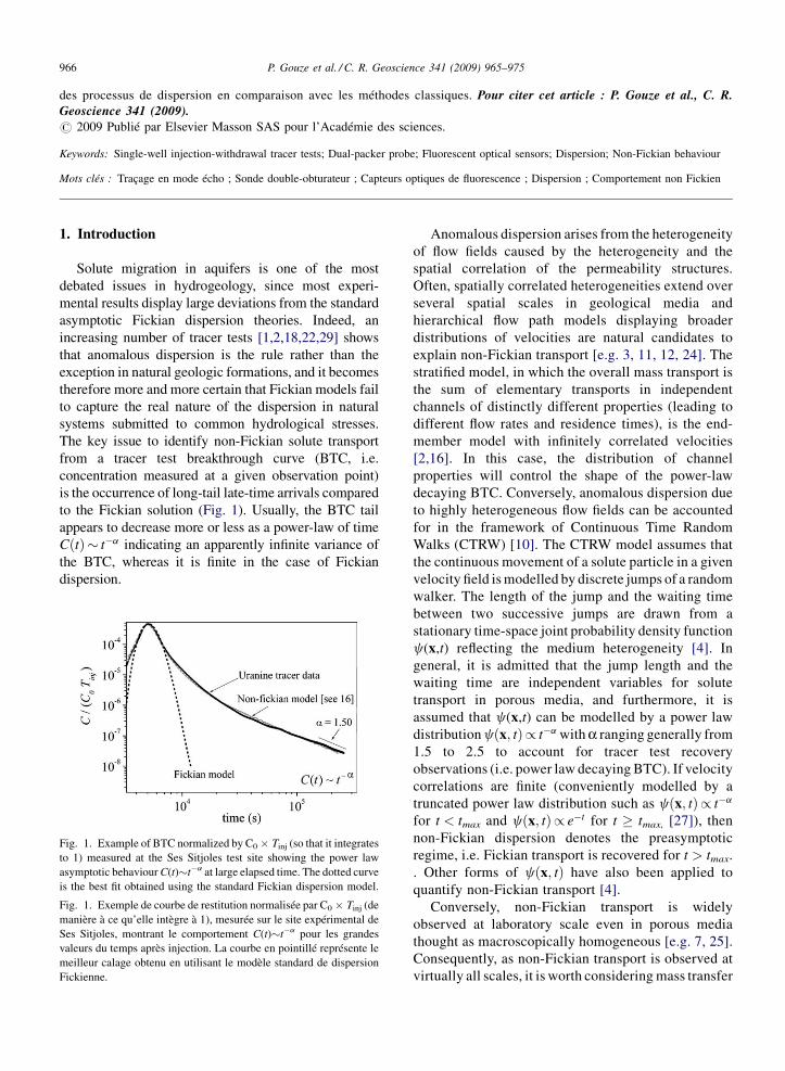

des processus de dispersion en comparaison avec les méthodes classiques. Pour citer cet article : P. Gouze et al., C. R.Geoscience 341 (2009).# 2009 Publié par Elsevier Masson SAS pour l’Académie des sciences.

Keywords: Single-well injection-withdrawal tracer tests; Dual-packer probe; Fluorescent optical sensors; Dispersion; Non-Fickian behaviour

Mots clés : Traçage en mode écho ; Sonde double-obturateur ; Capteurs optiques de fluorescence ; Dispersion ; Comportement non Fickien

P. Gouze et al. / C. R. Geoscience 341 (2009) 965–975966

1. Introduction

Solute migration in aquifers is one of the mostdebated issues in hydrogeology, since most experi-mental results display large deviations from the standardasymptotic Fickian dispersion theories. Indeed, anincreasing number of tracer tests [1,2,18,22,29] showsthat anomalous dispersion is the rule rather than theexception in natural geologic formations, and it becomestherefore more and more certain that Fickian models failto capture the real nature of the dispersion in naturalsystems submitted to common hydrological stresses.The key issue to identify non-Fickian solute transportfrom a tracer test breakthrough curve (BTC, i.e.concentration measured at a given observation point)is the occurrence of long-tail late-time arrivals comparedto the Fickian solution (Fig. 1). Usually, the BTC tailappears to decrease more or less as a power-law of timeCðtÞ� t�a indicating an apparently infinite variance ofthe BTC, whereas it is finite in the case of Fickiandispersion.

Fig. 1. Example of BTC normalized by C0 � Tinj (so that it integratesto 1) measured at the Ses Sitjoles test site showing the power lawasymptotic behaviour C(t)�t�a at large elapsed time. The dotted curveis the best fit obtained using the standard Fickian dispersion model.

Fig. 1. Exemple de courbe de restitution normalisée par C0 � Tinj (demanière à ce qu’elle intègre à 1), mesurée sur le site expérimental deSes Sitjoles, montrant le comportement C(t)�t�a pour les grandesvaleurs du temps après injection. La courbe en pointillé représente lemeilleur calage obtenu en utilisant le modèle standard de dispersionFickienne.

Anomalous dispersion arises from the heterogeneityof flow fields caused by the heterogeneity and thespatial correlation of the permeability structures.Often, spatially correlated heterogeneities extend overseveral spatial scales in geological media andhierarchical flow path models displaying broaderdistributions of velocities are natural candidates toexplain non-Fickian transport [e.g. 3, 11, 12, 24]. Thestratified model, in which the overall mass transport isthe sum of elementary transports in independentchannels of distinctly different properties (leading todifferent flow rates and residence times), is the end-member model with infinitely correlated velocities[2,16]. In this case, the distribution of channelproperties will control the shape of the power-lawdecaying BTC. Conversely, anomalous dispersion dueto highly heterogeneous flow fields can be accountedfor in the framework of Continuous Time RandomWalks (CTRW) [10]. The CTRW model assumes thatthe continuous movement of a solute particle in a givenvelocity field is modelled by discrete jumps of a randomwalker. The length of the jump and the waiting timebetween two successive jumps are drawn from astationary time-space joint probability density functionc(x,t) reflecting the medium heterogeneity [4]. Ingeneral, it is admitted that the jump length and thewaiting time are independent variables for solutetransport in porous media, and furthermore, it isassumed that c(x,t) can be modelled by a power lawdistribution cðx; tÞ/ t�a with a ranging generally from1.5 to 2.5 to account for tracer test recoveryobservations (i.e. power law decaying BTC). If velocitycorrelations are finite (conveniently modelled by atruncated power law distribution such as cðx; tÞ/ t�a

for t < tmax and cðx; tÞ/ e�t for t � tmax, [27]), thennon-Fickian dispersion denotes the preasymptoticregime, i.e. Fickian transport is recovered for t > tmax.. Other forms of cðx; tÞ have also been applied toquantify non-Fickian transport [4].

Conversely, non-Fickian transport is widelyobserved at laboratory scale even in porous mediathought as macroscopically homogeneous [e.g. 7, 25].Consequently, as non-Fickian transport is observed atvirtually all scales, it is worth considering mass transfer

P. Gouze et al. / C. R. Geoscience 341 (2009) 965–975 967

into small-scale geological structures where diffusiondominates as another possible origin of anomalousdispersion. For instance, the mobile-immobile multi-rate mass transfer (MIM) model assumes massexchanges between the moving fluid and a lesspermeable domain in which the fluid is considered asimmobile [6,8,15,17,31]. Here, non-Fickian transportis not controlled by the characteristics of the flowfield, but by the diffusion-controlled transport of thesolute particles in dead-end structures. The late-timeBTC concentration C(t) is proportional to the timederivative (noted G) of the so-called memory functionG(t) [18]:

CðtÞ � �tC0Tin jGðtÞ for t� t; (1)

where t is the average advective residence time of the

solute moving from the input to the observation location

and C0 is the concentration injected during the time

period Tinj. The memory function G(t) denotes the

inverse of the residence time distribution in the immo-

bile domain. If the late-time BTC displays a power law

decay with time, then both G(t) and the associated

probability density function c(t) for the CTRW model

are truncated power law distributions (here tmax corre-

sponds to the slower/longer diffusion path in the immo-

bile domain; e.g. [18]). Accordingly, the continuum

formulation for the MIM model is: C� LðCÞ ¼ C�G,

where C is the time derivative of the concentration

Cðx; tÞ in the flowing water, L(C) is the Fickian trans-

port operator (the divergence of the advection and

dispersion fluxes, see [9] for details) and notation

‘‘*’’ refers to the convolution product. The classical

Fickian advection-dispersion equation is retrieved for

G(t) = 0, i.e., no mass exchange with the immobile

domain or for t > tmax. The equivalence between the

MIM model with the memory function G and the

CTRW model with the transition time distribution C

is given in [10].

From the above discussion, it comes out that bothwater velocity heterogeneity controlled by large-scalestructures and diffusion processes controlled by small-scale structures lead to anomalous transport and similarpower-law decaying BTCs. Furthermore, they are bothequivalently modelled by CTRW using a power lawdecaying distribution of the waiting time, for instance.However, the discrimination between the control of thelarge-scale heterogeneity of the permeability field andthat of the small-scale diffusion-controlled structures isa critical issue for model parameterisation andupscaling. Yet, it is a difficult task because it is mostprobable that both may be present simultaneously inseveral heterogeneous reservoirs. Nevertheless, it is

possible of minimizing the velocity spatial correlationusing Single-Well Injection-Withdrawal (SWIW) tracertests and by selecting reservoir targets displaying large-scale homogeneity.

SWIW tracer tests, also called push-pull tracer tests,consist in injecting a given mass of tracer in themedium and reversing the flow after a certain time inorder to measure the tracer breakthrough curve at theinjection point [13,19,33]. This technique presentsseveral advantages. First, the reversal of flow warrantsan optimal tracer mass recovery, which is ofimportance to produce quantitative results. Second,the SWIW tracer test allows measuring the irreversibledispersion (or mixing) whereas the reversible disper-sion (i.e., the spreading induced by a long-rangecorrelated path) taking place during the tracer pushphase is cancelled during the withdrawal phase [2,21].The quantification of the reversible and irreversibledispersion refers to a given scale of observation which,in our case, is the maximal distance migrated by thetracer during the SWIW tracer test. More precisely,velocity correlation, over distances smaller than theexploration size, will result in irreversible dispersion(diffusion and mixing) whereas advection spreadingdue to velocity correlation larger than the explorationsize will be cancelled (see Fig. 1 in [14]). Thus, thedispersion measured using SWIW tests is only causedby tracer molecules that do not follow the same path inthe injection and the withdrawal phases. In this case,the observation of non-Fickian transport may indicatethe occurrence of mass transfers into immobile zones.Third, using SWIW tests, the tracer may be pushed atdifferent distances from the injection point, thusvisiting different volumes of the system using a singlewell. This allows investigating the dispersion pro-cesses for increasing volumes of reservoir [23],studying the scale effect on dispersion, and subse-quently testing the different assumptions concerningthe origin of the anomalous dispersion (i.e. scale-dependent flow velocity heterogeneity versus porescale diffusion models).

In theory, all the information required to characterizethe anomalous dispersion can be retrieved from theBTC shape and specifically from the BTC tailing.However, in practice, it is generally difficult to evaluatewhether the observed BTC tail represents the rate-limited behaviour only or a transitional behaviour in thevicinity of the main concentration peak, unlessconcentration is measured for long times after theadvection peak has passed. Therefore, long-lastingrecording of the tracer recovery and high-resolutionsensors are required. In practice, the concentration must

P. Gouze et al. / C. R. Geoscience 341 (2009) 965–975968

be measured over several orders of magnitude (4 to 5generally).

The aim of this article is to present new equipmentrecently developed to investigate (anomalous) disper-sion from laboratory to field scale. First, we will focuson pointing out the capacity of the fluorescent sensorTELog to produce unmatched in situ high resolutionfluorescent dyes concentration monitoring. Second,we will describe the downhole probe CoFIS that isdesigned to perform fully controlled, long-lastingSWIW tracer tests. Finally, some examples of resultsof tracer tests in fractured and porous media arepresented.

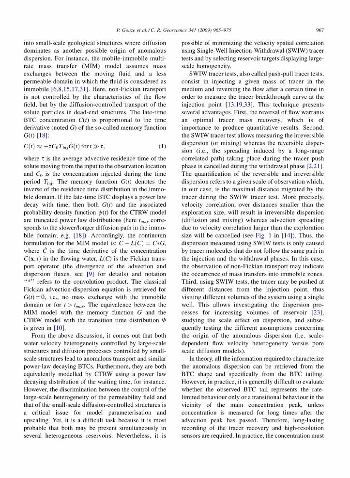
Fig. 2. a: Schematic representation of the CoFIS probe (the horizontal scalethe TELog sensor that is installed in the CoFIS probe for fluorescent dye moptical path. The recurrent measurement of two different fluorescent tracerscomputer-controlled rotation of the band-pass filter holder, while activating oa 485 10 nm excitation filter and a 530 12 nm emission filter, sulforho590 17 nm emission filter, turbidity is measured at 530 12 nm and LEDchamber.

Fig. 2. a : représentation schématique de la sonde CoFIS (l’échelle horizonreprésentation schématique de la sonde TELog qui est installée dans la sondétails du système optique de la sonde TELog. La mesure récurrente de deuxpar la rotation, contrôlée par microprocesseurs, du barillet où sont installés lesl’uranine est mesuré avec un filtre d’excitation à 485 10 nm et un filtre d’émun filtre d’excitation à 530 12 nm et un filtre d’émission à 590 17 nm; lLED est mesuré grâce à un guide de lumière permettant de bipasser la zon

2. Equipment and methodology

2.1. Fluorescent dye measurement using the TELogtool

For measuring dispersion of a passive tracer, it isessential to use low concentrations of tracer in order toavoid density effects [32], while ensuring that the tracerconcentration can be measured over four orders ofmagnitude, at least. A specific high-resolution sensor,called TELog, was developed to account for theserequirements. In TELog, uranine and sulforhodaminfluorescent dyes and turbidity are measured using a set

is exaggerated for better visualization); b: Schematic representation ofeasurement; c: details of the TELog measurement head displaying the(e.g. uranine and sulforhodamine) and water turbidity is performed byne of the two pulsed-led light sources. Uranine signal is measured withdamine signal is measured with a 530 12 nm excitation filter and as intensity is measured using a light-guide bypassing the measurement

tale est exagérée pour une meilleure visualisation des éléments) ; b :de CoFIS pour mesurer la concentration en traceurs fluorescents ; c :traceurs (ex : uranine et sulforhodamine) et de la turbidité est réaliséefiltres et des deux LED pulsées qui fournissent la lumière. Le signal deission à 530 12 nm ; le signal de la sulforhodamine est mesuré avec

e signal de turbidité est mesuré à 530 12 nm et l’intensité de chaquee de mesure du fluide.

P. Gouze et al. / C. R. Geoscience 341 (2009) 965–975 969

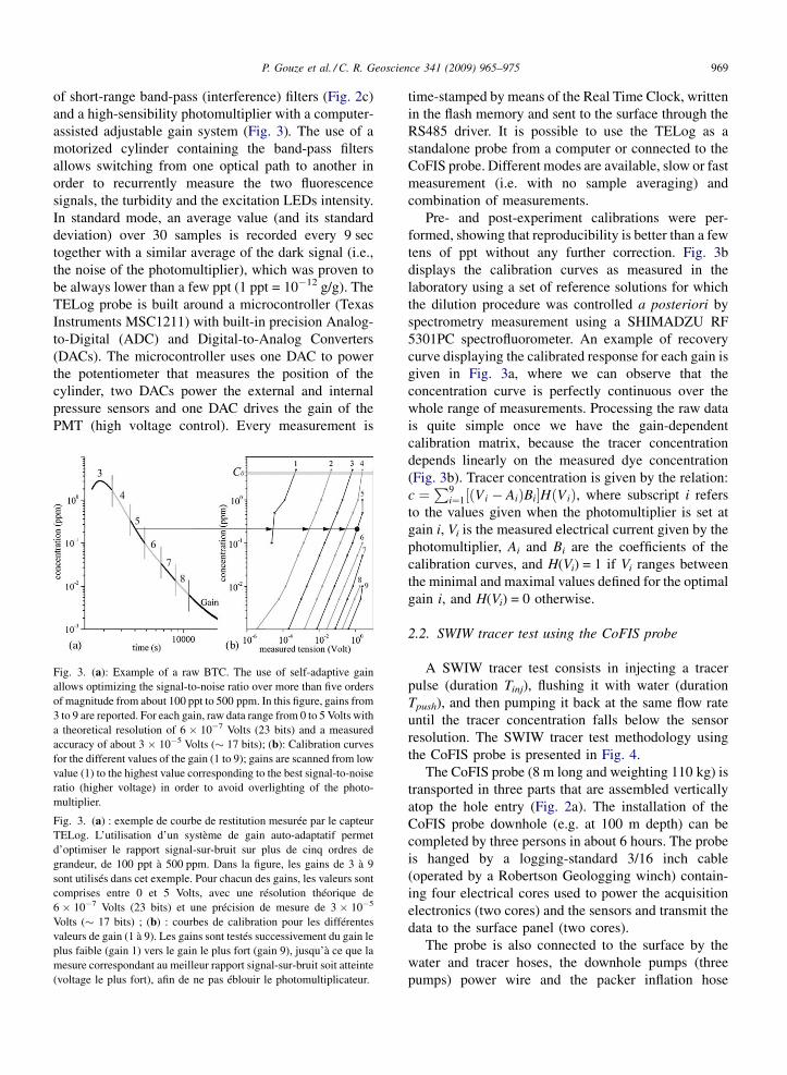
of short-range band-pass (interference) filters (Fig. 2c)and a high-sensibility photomultiplier with a computer-assisted adjustable gain system (Fig. 3). The use of amotorized cylinder containing the band-pass filtersallows switching from one optical path to another inorder to recurrently measure the two fluorescencesignals, the turbidity and the excitation LEDs intensity.In standard mode, an average value (and its standarddeviation) over 30 samples is recorded every 9 sectogether with a similar average of the dark signal (i.e.,the noise of the photomultiplier), which was proven tobe always lower than a few ppt (1 ppt = 10�12 g/g). TheTELog probe is built around a microcontroller (TexasInstruments MSC1211) with built-in precision Analog-to-Digital (ADC) and Digital-to-Analog Converters(DACs). The microcontroller uses one DAC to powerthe potentiometer that measures the position of thecylinder, two DACs power the external and internalpressure sensors and one DAC drives the gain of thePMT (high voltage control). Every measurement is

Fig. 3. (a): Example of a raw BTC. The use of self-adaptive gainallows optimizing the signal-to-noise ratio over more than five ordersof magnitude from about 100 ppt to 500 ppm. In this figure, gains from3 to 9 are reported. For each gain, raw data range from 0 to 5 Volts witha theoretical resolution of 6 � 10�7 Volts (23 bits) and a measuredaccuracy of about 3 � 10�5 Volts (� 17 bits); (b): Calibration curvesfor the different values of the gain (1 to 9); gains are scanned from lowvalue (1) to the highest value corresponding to the best signal-to-noiseratio (higher voltage) in order to avoid overlighting of the photo-multiplier.

Fig. 3. (a) : exemple de courbe de restitution mesurée par le capteurTELog. L’utilisation d’un système de gain auto-adaptatif permetd’optimiser le rapport signal-sur-bruit sur plus de cinq ordres degrandeur, de 100 ppt à 500 ppm. Dans la figure, les gains de 3 à 9sont utilisés dans cet exemple. Pour chacun des gains, les valeurs sontcomprises entre 0 et 5 Volts, avec une résolution théorique de6 � 10�7 Volts (23 bits) et une précision de mesure de 3 � 10�5

Volts (� 17 bits) ; (b) : courbes de calibration pour les différentesvaleurs de gain (1 à 9). Les gains sont testés successivement du gain leplus faible (gain 1) vers le gain le plus fort (gain 9), jusqu’à ce que lamesure correspondant au meilleur rapport signal-sur-bruit soit atteinte(voltage le plus fort), afin de ne pas éblouir le photomultiplicateur.

time-stamped by means of the Real Time Clock, writtenin the flash memory and sent to the surface through theRS485 driver. It is possible to use the TELog as astandalone probe from a computer or connected to theCoFIS probe. Different modes are available, slow or fastmeasurement (i.e. with no sample averaging) andcombination of measurements.

Pre- and post-experiment calibrations were per-formed, showing that reproducibility is better than a fewtens of ppt without any further correction. Fig. 3bdisplays the calibration curves as measured in thelaboratory using a set of reference solutions for whichthe dilution procedure was controlled a posteriori byspectrometry measurement using a SHIMADZU RF5301PC spectrofluorometer. An example of recoverycurve displaying the calibrated response for each gain isgiven in Fig. 3a, where we can observe that theconcentration curve is perfectly continuous over thewhole range of measurements. Processing the raw datais quite simple once we have the gain-dependentcalibration matrix, because the tracer concentrationdepends linearly on the measured dye concentration(Fig. 3b). Tracer concentration is given by the relation:c ¼

P9i¼1 ðVi � AiÞBi½ HðViÞ, where subscript i refers

to the values given when the photomultiplier is set atgain i, Vi is the measured electrical current given by thephotomultiplier, Ai and Bi are the coefficients of thecalibration curves, and H(Vi) = 1 if Vi ranges betweenthe minimal and maximal values defined for the optimalgain i, and H(Vi) = 0 otherwise.

2.2. SWIW tracer test using the CoFIS probe

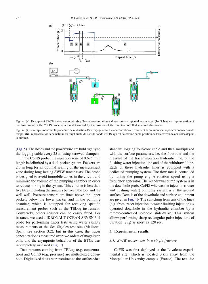
A SWIW tracer test consists in injecting a tracerpulse (duration Tinj), flushing it with water (durationTpush), and then pumping it back at the same flow rateuntil the tracer concentration falls below the sensorresolution. The SWIW tracer test methodology usingthe CoFIS probe is presented in Fig. 4.

The CoFIS probe (8 m long and weighting 110 kg) istransported in three parts that are assembled verticallyatop the hole entry (Fig. 2a). The installation of theCoFIS probe downhole (e.g. at 100 m depth) can becompleted by three persons in about 6 hours. The probeis hanged by a logging-standard 3/16 inch cable(operated by a Robertson Geologging winch) contain-ing four electrical cores used to power the acquisitionelectronics (two cores) and the sensors and transmit thedata to the surface panel (two cores).

The probe is also connected to the surface by thewater and tracer hoses, the downhole pumps (threepumps) power wire and the packer inflation hose

P. Gouze et al. / C. R. Geoscience 341 (2009) 965–975970

Fig. 4. (a): Example of SWIW tracer test monitoring. Tracer concentration and pressure are reported versus time; (b): Schematic representation ofthe flow circuit in the CoFIS probe which is determined by the position of the remote-controlled solenoid slide-valve.

Fig. 4. (a) : exemple montrant la procédure de réalisation d’un traçage écho. La concentration en traceur et la pression sont reportées en fonction dutemps ; (b) : représentation schématique du trajet du fluide dans la sonde CoFIS, qui est déterminé par la position de l’électrovanne contrôlée depuisla surface.

(Fig. 5). The hoses and the power wire are hold tightly tothe logging cable every 25 m using screwed clampers.

In the CoFIS probe, the injection zone of 0.675 m inlength is delimited by a dual-packer system. Packers are2.5 m long for an optimal sealing of the measurementzone during long-lasting SWIW tracer tests. The probeis designed to avoid immobile zones in the circuit andminimize the volume of the pumping chamber in orderto reduce mixing in the system. This volume is less thanfive litres including the annulus between the tool and thewell wall. Pressure sensors are fitted above the upperpacker, below the lower packer and in the pumpingchamber, which is equipped for receiving specificmeasurement probes such as the TELog instrument.Conversely, others sensors can be easily fitted. Forinstance, we used a IDRONAUT OCEAN-SEVEN 304probe for performing tracer tests using water salinitymeasurements at the Ses Sitjoles test site (Mallorca,Spain, see section 3.2), but in this case, the tracerconcentration is measured over two orders of magnitudeonly, and the asymptotic behaviour of the BTCs wasincompletely assessed (Fig. 7).

Data streams coming from TELog (e.g. concentra-tion) and CoFIS (e.g. pressure) are multiplexed down-hole. Digitalized data are transmitted to the surface via a

standard logging four-core cable and then multiplexedwith the surface parameters, i.e. the flow rate and thepressure of the tracer injection hydraulic line, of theflushing water injection line and of the withdrawal line.Each of these hydraulic lines is equipped with adedicated pumping system. The flow rate is controlledby tuning the pump engine rotation speed using afrequency generator. The withdrawal pump system is inthe downhole probe CoFIS whereas the injection (tracerand flushing water) pumping system is at the groundsurface. Details of the downhole and surface equipmentare given in Fig. 4b. The switching from any of the lines(e.g. from tracer injection to water flushing injection) isoperated downhole in the hydraulic chamber by aremote-controlled solenoid slide-valve. This systemallows performing sharp rectangular pulse injections ofduration (Tinj) as short as 120 sec.

3. Experimental results

3.1. SWIW tracer tests in a single fracture

CoFIS was first deployed at the Lavalette experi-mental site, which is located 3 km away from theMontpellier University campus (France). The test site

P. Gouze et al. / C. R. Geoscience 341 (2009) 965–975 971

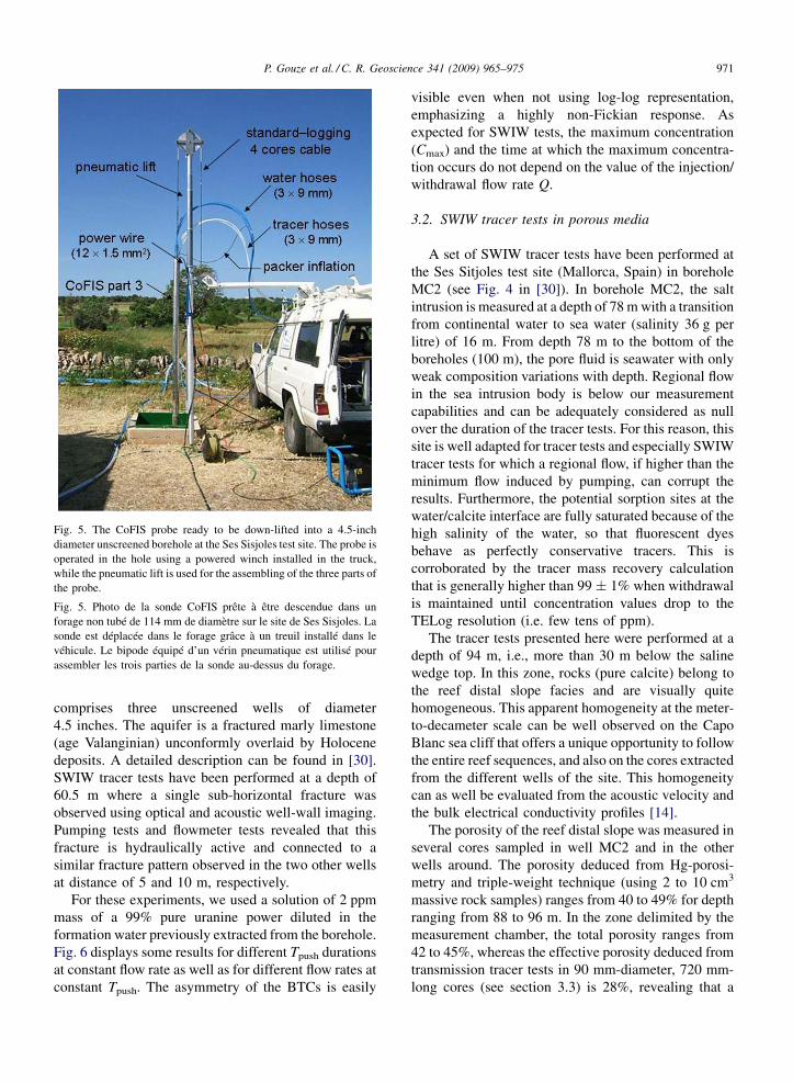
Fig. 5. The CoFIS probe ready to be down-lifted into a 4.5-inchdiameter unscreened borehole at the Ses Sisjoles test site. The probe isoperated in the hole using a powered winch installed in the truck,while the pneumatic lift is used for the assembling of the three parts ofthe probe.

Fig. 5. Photo de la sonde CoFIS prête à être descendue dans unforage non tubé de 114 mm de diamètre sur le site de Ses Sisjoles. Lasonde est déplacée dans le forage grâce à un treuil installé dans levéhicule. Le bipode équipé d’un vérin pneumatique est utilisé pourassembler les trois parties de la sonde au-dessus du forage.

comprises three unscreened wells of diameter4.5 inches. The aquifer is a fractured marly limestone(age Valanginian) unconformly overlaid by Holocenedeposits. A detailed description can be found in [30].SWIW tracer tests have been performed at a depth of60.5 m where a single sub-horizontal fracture wasobserved using optical and acoustic well-wall imaging.Pumping tests and flowmeter tests revealed that thisfracture is hydraulically active and connected to asimilar fracture pattern observed in the two other wellsat distance of 5 and 10 m, respectively.

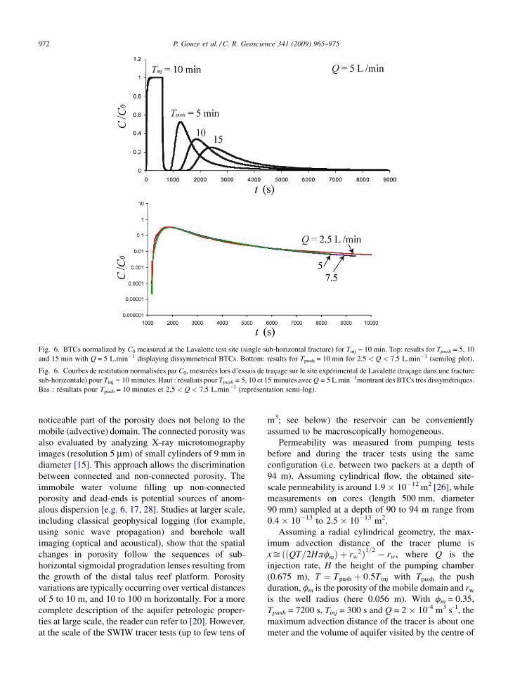
For these experiments, we used a solution of 2 ppmmass of a 99% pure uranine power diluted in theformation water previously extracted from the borehole.Fig. 6 displays some results for different Tpush durationsat constant flow rate as well as for different flow rates atconstant Tpush. The asymmetry of the BTCs is easily

visible even when not using log-log representation,emphasizing a highly non-Fickian response. Asexpected for SWIW tests, the maximum concentration(Cmax) and the time at which the maximum concentra-tion occurs do not depend on the value of the injection/withdrawal flow rate Q.

3.2. SWIW tracer tests in porous media

A set of SWIW tracer tests have been performed atthe Ses Sitjoles test site (Mallorca, Spain) in boreholeMC2 (see Fig. 4 in [30]). In borehole MC2, the saltintrusion is measured at a depth of 78 m with a transitionfrom continental water to sea water (salinity 36 g perlitre) of 16 m. From depth 78 m to the bottom of theboreholes (100 m), the pore fluid is seawater with onlyweak composition variations with depth. Regional flowin the sea intrusion body is below our measurementcapabilities and can be adequately considered as nullover the duration of the tracer tests. For this reason, thissite is well adapted for tracer tests and especially SWIWtracer tests for which a regional flow, if higher than theminimum flow induced by pumping, can corrupt theresults. Furthermore, the potential sorption sites at thewater/calcite interface are fully saturated because of thehigh salinity of the water, so that fluorescent dyesbehave as perfectly conservative tracers. This iscorroborated by the tracer mass recovery calculationthat is generally higher than 99 1% when withdrawalis maintained until concentration values drop to theTELog resolution (i.e. few tens of ppm).

The tracer tests presented here were performed at adepth of 94 m, i.e., more than 30 m below the salinewedge top. In this zone, rocks (pure calcite) belong tothe reef distal slope facies and are visually quitehomogeneous. This apparent homogeneity at the meter-to-decameter scale can be well observed on the CapoBlanc sea cliff that offers a unique opportunity to followthe entire reef sequences, and also on the cores extractedfrom the different wells of the site. This homogeneitycan as well be evaluated from the acoustic velocity andthe bulk electrical conductivity profiles [14].

The porosity of the reef distal slope was measured inseveral cores sampled in well MC2 and in the otherwells around. The porosity deduced from Hg-porosi-metry and triple-weight technique (using 2 to 10 cm3

massive rock samples) ranges from 40 to 49% for depthranging from 88 to 96 m. In the zone delimited by themeasurement chamber, the total porosity ranges from42 to 45%, whereas the effective porosity deduced fromtransmission tracer tests in 90 mm-diameter, 720 mm-long cores (see section 3.3) is 28%, revealing that a

P. Gouze et al. / C. R. Geoscience 341 (2009) 965–975972

Fig. 6. BTCs normalized by C0 measured at the Lavalette test site (single sub-horizontal fracture) for Tinj = 10 min. Top: results for Tpush = 5, 10and 15 min with Q = 5 L.min�1 displaying dissymmetrical BTCs. Bottom: results for Tpush = 10 min for 2.5 < Q < 7.5 L.min�1 (semilog plot).

Fig. 6. Courbes de restitution normalisées par C0, mesurées lors d’essais de traçage sur le site expérimental de Lavalette (traçage dans une fracturesub-horizontale) pour Tinj = 10 minutes. Haut : résultats pour Tpush = 5, 10 et 15 minutes avec Q = 5 L.min�1montrant des BTCs très dissymétriques.Bas : résultats pour Tpush = 10 minutes et 2,5 < Q < 7,5 L.min�1 (représentation semi-log).

noticeable part of the porosity does not belong to themobile (advective) domain. The connected porosity wasalso evaluated by analyzing X-ray microtomographyimages (resolution 5 mm) of small cylinders of 9 mm indiameter [15]. This approach allows the discriminationbetween connected and non-connected porosity. Theimmobile water volume filling up non-connectedporosity and dead-ends is potential sources of anom-alous dispersion [e.g. 6, 17, 28]. Studies at larger scale,including classical geophysical logging (for example,using sonic wave propagation) and borehole wallimaging (optical and acoustical), show that the spatialchanges in porosity follow the sequences of sub-horizontal sigmoidal progradation lenses resulting fromthe growth of the distal talus reef platform. Porosityvariations are typically occurring over vertical distancesof 5 to 10 m, and 10 to 100 m horizontally. For a morecomplete description of the aquifer petrologic proper-ties at large scale, the reader can refer to [20]. However,at the scale of the SWIW tracer tests (up to few tens of

m3; see below) the reservoir can be convenientlyassumed to be macroscopically homogeneous.

Permeability was measured from pumping testsbefore and during the tracer tests using the sameconfiguration (i.e. between two packers at a depth of94 m). Assuming cylindrical flow, the obtained site-scale permeability is around 1.9 � 10�12 m2 [26], whilemeasurements on cores (length 500 mm, diameter90 mm) sampled at a depth of 90 to 94 m range from0.4 � 10�13 to 2.5 � 10�13 m2.

Assuming a radial cylindrical geometry, the max-imum advection distance of the tracer plume isxffi QT=2Hpfmð Þ þ rw

2ð Þ1=2 � rw, where Q is theinjection rate, H the height of the pumping chamber(0.675 m), T ¼ Tpush þ 0:5T inj with Tpush the pushduration, fm is the porosity of the mobile domain and rw

is the well radius (here 0.056 m). With fm = 0.35,Tpush = 7200 s, Tinj = 300 s and Q = 2 � 10-4 m3 s-1, themaximum advection distance of the tracer is about onemeter and the volume of aquifer visited by the centre of

P. Gouze et al. / C. R. Geoscience 341 (2009) 965–975 973

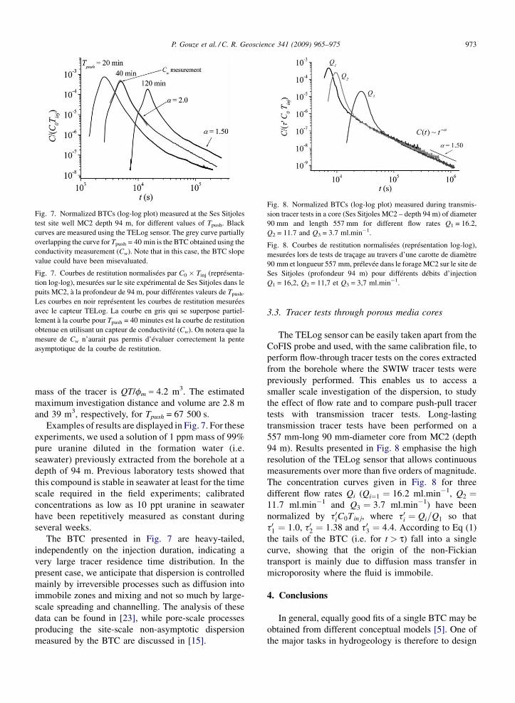
Fig. 7. Normalized BTCs (log-log plot) measured at the Ses Sitjolestest site well MC2 depth 94 m, for different values of Tpush. Blackcurves are measured using the TELog sensor. The grey curve partiallyoverlapping the curve for Tpush = 40 min is the BTC obtained using theconductivity measurement (Cw). Note that in this case, the BTC slopevalue could have been misevaluated.

Fig. 7. Courbes de restitution normalisées par C0 � Tinj (représenta-tion log-log), mesurées sur le site expérimental de Ses Sitjoles dans lepuits MC2, à la profondeur de 94 m, pour différentes valeurs de Tpush.Les courbes en noir représentent les courbes de restitution mesuréesavec le capteur TELog. La courbe en gris qui se superpose partiel-lement à la courbe pour Tpush = 40 minutes est la courbe de restitutionobtenue en utilisant un capteur de conductivité (Cw). On notera que lamesure de Cw n’aurait pas permis d’évaluer correctement la penteasymptotique de la courbe de restitution.

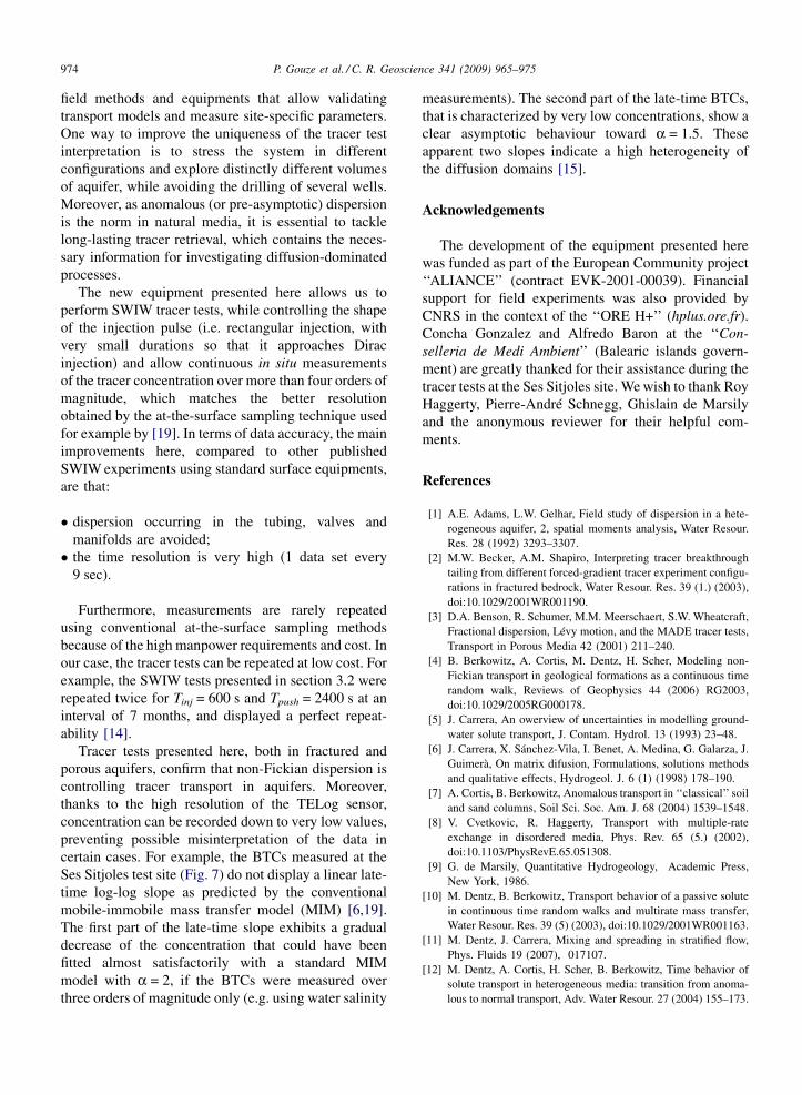
Fig. 8. Normalized BTCs (log-log plot) measured during transmis-sion tracer tests in a core (Ses Sitjoles MC2 – depth 94 m) of diameter90 mm and length 557 mm for different flow rates Q1 = 16.2,Q2 = 11.7 and Q3 = 3.7 ml.min�1.

Fig. 8. Courbes de restitution normalisées (représentation log-log),mesurées lors de tests de traçage au travers d’une carotte de diamètre90 mm et longueur 557 mm, prélevée dans le forage MC2 sur le site deSes Sitjoles (profondeur 94 m) pour différents débits d’injectionQ1 = 16,2, Q2 = 11,7 et Q3 = 3,7 ml.min�1.

mass of the tracer is QT/fm = 4.2 m3. The estimatedmaximum investigation distance and volume are 2.8 mand 39 m3, respectively, for Tpush = 67 500 s.

Examples of results are displayed in Fig. 7. For theseexperiments, we used a solution of 1 ppm mass of 99%pure uranine diluted in the formation water (i.e.seawater) previously extracted from the borehole at adepth of 94 m. Previous laboratory tests showed thatthis compound is stable in seawater at least for the timescale required in the field experiments; calibratedconcentrations as low as 10 ppt uranine in seawaterhave been repetitively measured as constant duringseveral weeks.

The BTC presented in Fig. 7 are heavy-tailed,independently on the injection duration, indicating avery large tracer residence time distribution. In thepresent case, we anticipate that dispersion is controlledmainly by irreversible processes such as diffusion intoimmobile zones and mixing and not so much by large-scale spreading and channelling. The analysis of thesedata can be found in [23], while pore-scale processesproducing the site-scale non-asymptotic dispersionmeasured by the BTC are discussed in [15].

3.3. Tracer tests through porous media cores

The TELog sensor can be easily taken apart from theCoFIS probe and used, with the same calibration file, toperform flow-through tracer tests on the cores extractedfrom the borehole where the SWIW tracer tests werepreviously performed. This enables us to access asmaller scale investigation of the dispersion, to studythe effect of flow rate and to compare push-pull tracertests with transmission tracer tests. Long-lastingtransmission tracer tests have been performed on a557 mm-long 90 mm-diameter core from MC2 (depth94 m). Results presented in Fig. 8 emphasise the highresolution of the TELog sensor that allows continuousmeasurements over more than five orders of magnitude.The concentration curves given in Fig. 8 for threedifferent flow rates Qi (Qi¼1 ¼ 16:2 ml.min�1, Q2 ¼11:7 ml.min�1 and Q3 ¼ 3:7 ml.min�1) have beennormalized by t0iC0Tin j, where t0i ¼ Qi=Q1 so thatt01 ¼ 1:0, t02 ¼ 1:38 and t03 ¼ 4:4. According to Eq (1)the tails of the BTC (i.e. for t > t) fall into a singlecurve, showing that the origin of the non-Fickiantransport is mainly due to diffusion mass transfer inmicroporosity where the fluid is immobile.

4. Conclusions

In general, equally good fits of a single BTC may beobtained from different conceptual models [5]. One ofthe major tasks in hydrogeology is therefore to design

P. Gouze et al. / C. R. Geoscience 341 (2009) 965–975974

field methods and equipments that allow validatingtransport models and measure site-specific parameters.One way to improve the uniqueness of the tracer testinterpretation is to stress the system in differentconfigurations and explore distinctly different volumesof aquifer, while avoiding the drilling of several wells.Moreover, as anomalous (or pre-asymptotic) dispersionis the norm in natural media, it is essential to tacklelong-lasting tracer retrieval, which contains the neces-sary information for investigating diffusion-dominatedprocesses.

The new equipment presented here allows us toperform SWIW tracer tests, while controlling the shapeof the injection pulse (i.e. rectangular injection, withvery small durations so that it approaches Diracinjection) and allow continuous in situ measurementsof the tracer concentration over more than four orders ofmagnitude, which matches the better resolutionobtained by the at-the-surface sampling technique usedfor example by [19]. In terms of data accuracy, the mainimprovements here, compared to other publishedSWIW experiments using standard surface equipments,are that:

� dispersion occurring in the tubing, valves andmanifolds are avoided;� the time resolution is very high (1 data set every

9 sec).

Furthermore, measurements are rarely repeatedusing conventional at-the-surface sampling methodsbecause of the high manpower requirements and cost. Inour case, the tracer tests can be repeated at low cost. Forexample, the SWIW tests presented in section 3.2 wererepeated twice for Tinj = 600 s and Tpush = 2400 s at aninterval of 7 months, and displayed a perfect repeat-ability [14].

Tracer tests presented here, both in fractured andporous aquifers, confirm that non-Fickian dispersion iscontrolling tracer transport in aquifers. Moreover,thanks to the high resolution of the TELog sensor,concentration can be recorded down to very low values,preventing possible misinterpretation of the data incertain cases. For example, the BTCs measured at theSes Sitjoles test site (Fig. 7) do not display a linear late-time log-log slope as predicted by the conventionalmobile-immobile mass transfer model (MIM) [6,19].The first part of the late-time slope exhibits a gradualdecrease of the concentration that could have beenfitted almost satisfactorily with a standard MIMmodel with a = 2, if the BTCs were measured overthree orders of magnitude only (e.g. using water salinity

measurements). The second part of the late-time BTCs,that is characterized by very low concentrations, show aclear asymptotic behaviour toward a = 1.5. Theseapparent two slopes indicate a high heterogeneity ofthe diffusion domains [15].

Acknowledgements

The development of the equipment presented herewas funded as part of the European Community project‘‘ALIANCE’’ (contract EVK-2001-00039). Financialsupport for field experiments was also provided byCNRS in the context of the ‘‘ORE H+’’ (hplus.ore.fr).Concha Gonzalez and Alfredo Baron at the ‘‘Con-selleria de Medi Ambient’’ (Balearic islands govern-ment) are greatly thanked for their assistance during thetracer tests at the Ses Sitjoles site. We wish to thank RoyHaggerty, Pierre-André Schnegg, Ghislain de Marsilyand the anonymous reviewer for their helpful com-ments.

References

[1] A.E. Adams, L.W. Gelhar, Field study of dispersion in a hete-rogeneous aquifer, 2, spatial moments analysis, Water Resour.Res. 28 (1992) 3293–3307.

[2] M.W. Becker, A.M. Shapiro, Interpreting tracer breakthroughtailing from different forced-gradient tracer experiment configu-rations in fractured bedrock, Water Resour. Res. 39 (1.) (2003),doi:10.1029/2001WR001190.

[3] D.A. Benson, R. Schumer, M.M. Meerschaert, S.W. Wheatcraft,Fractional dispersion, Lévy motion, and the MADE tracer tests,Transport in Porous Media 42 (2001) 211–240.

[4] B. Berkowitz, A. Cortis, M. Dentz, H. Scher, Modeling non-Fickian transport in geological formations as a continuous timerandom walk, Reviews of Geophysics 44 (2006) RG2003,doi:10.1029/2005RG000178.

[5] J. Carrera, An owerview of uncertainties in modelling ground-water solute transport, J. Contam. Hydrol. 13 (1993) 23–48.

[6] J. Carrera, X. Sánchez-Vila, I. Benet, A. Medina, G. Galarza, J.Guimerà, On matrix difusion, Formulations, solutions methodsand qualitative effects, Hydrogeol. J. 6 (1) (1998) 178–190.

[7] A. Cortis, B. Berkowitz, Anomalous transport in ‘‘classical’’ soiland sand columns, Soil Sci. Soc. Am. J. 68 (2004) 1539–1548.

[8] V. Cvetkovic, R. Haggerty, Transport with multiple-rateexchange in disordered media, Phys. Rev. 65 (5.) (2002),doi:10.1103/PhysRevE.65.051308.

[9] G. de Marsily, Quantitative Hydrogeology, Academic Press,New York, 1986.

[10] M. Dentz, B. Berkowitz, Transport behavior of a passive solutein continuous time random walks and multirate mass transfer,Water Resour. Res. 39 (5) (2003), doi:10.1029/2001WR001163.

[11] M. Dentz, J. Carrera, Mixing and spreading in stratified flow,Phys. Fluids 19 (2007), 017107.

[12] M. Dentz, A. Cortis, H. Scher, B. Berkowitz, Time behavior ofsolute transport in heterogeneous media: transition from anoma-lous to normal transport, Adv. Water Resour. 27 (2004) 155–173.

P. Gouze et al. / C. R. Geoscience 341 (2009) 965–975 975

[13] L.W. Gelhar, M.A. Collins, General analysis of longitudinaldispersion in nonuniform flow, Water Resour. Res. 7 (6) (1971)1511–1521.

[14] P. Gouze, T. Le Borgne, R. Leprovost, G. Lods, T. Poidras, P.A.Pezard, Non-Fickian dispersion in porous media: 1. Multiscalemeasurements using single-well injection withdrawal tracertests, Water Resour. Res. 44 (2008), doi:10.1029/2007WR006278 (W06427).

[15] P. Gouze, Y. Melean, T. Le Borgne, M. Dentz, J. Carrera, Non-Fickian dispersion in porous media explained by heterogeneousmicroscale matrix diffusion, Water Resour. Res. 44 (2008)W11416, doi:10.1029/2007WR006690.

[16] B.L. Gylling, L. Moreno, I. Neretnieks, The Channel NetworkModel - A tool for transport simulation in fractured media,Groundwater 37 (3) (1999) 367–375.

[17] R. Haggerty, S.M. Gorelick, Multiple-rate mass transfer formodeling diffusion and surface reactions in media with pore-scale heterogeneity, Water Resour. Res. 31 (10) (1995) 2383–

2400.[18] R. Haggerty, S.A. McKenna, L.C. Meigs, On the late-time

behavior of tracer test breakthrough curves, Water Resour.Res. 36 (12) (2000) 3467–3480.

[19] R. Haggerty, S.W. Fleming, L.C. Meigs, S.A. McKenna, Tracertests in a fractured dolomite, 2, Analysis of mass transfer insingle-well injection-withdrawal tests, Water Resour. Res. 37 (5)(2001) 1129–1142.

[20] D. Jaeggi, Multiscalar porosity structure of a Miocene reefalcarbonate complex, Diss., Naturwissenschaften, EidgenössischeTechnische Hochschule ETH Zürich, Nr. 16519 (2006).

[21] A.A. Khrapitchev, P.T. Callaghan, Reversible and irreversibledispersion in a porous medium, Phys. Fluids 15 (2003) 2649–

2660.[22] D.R. LeBlanc, S.P. Garabedian, K.M. Hess, L.W. Gelhar, R.D.

Quadri, K.G. Stollenwerk, W.W. Wood, Large-scale naturalgradient test in sand and gravel, Cape Cod, Massachusetts, 1:Experimental design and observed movement, Water Resour.Res. 27 (5) (1991) 885–910.

[23] T. Le Borgne, P. Gouze, Non-Fickian dispersion in porousmedia: 2. Model validation from measurements at differentscales, Water Resour. Res. 44 (2008), doi:10.1029/2007WR006279.

[24] T. Le Borgne, M. Dentz, J. Carrera, Lagrangian statistical modelfor transport in highly heterogeneous velocity fields, Phys. Rev.Lett. (2008) 101, doi:10.1103/PRL101.090601.

[25] M. Levy, B. Berkowitz, Measurement and analysis of non-Fickian dispersion in heterogeneous porous media, J. Contam.Hydrol. 64 (3–4) (2003) 203–226.

[26] G. Lods, P. Gouze, WTFM, a software for well tests analysis infractured media combining fractional flow with double porosityand leakance, Computer and Geosciences 30 (2004) 937–947.

[27] G. Margolin, B. Berkowitz, Application of continuous timerandom walks to transport in porous media, J. Phys. Chem.B104 (16) (2000) 3942–3947 (with a minor correction, publis-hed in J. Phys. Chem. B104[36] 8762).

[28] S.A. McKenna, L. Meigs, R. Haggerty, Tests in a fractureddolomite, 3, double-prosity, multiple-rate mass transfer proces-ses in convergent flow tracer tests, Water Resour. Res. 37 (5)(2001) 1143–1154.

[29] L.C. Meigs, R.L. Beauheim, Tracer tests in a fractured dolomite,1, Experimental design and observed tracer recoveries, WaterResour. Res. 37 (5) (2001) 1113–1128.

[30] P.A. Pezard, S. Gautier, T. Le Borgne, B. Legros, J.C. Deltombe,MuSET: a multiparameter and high precision sensor for down-hole spontaneous electrical potential measurements, C. R. Geos-cience (this issue); DOI: 10.1016/j.crte.2009.07.009.

[31] R. Schumer, D.A. Benson, M.M. Meerschaert, B. Baeumer,Fractal mobile/immobile solute transport, Water Resour. Res.39 (10) (2003), doi:10.1029/2003WR002141.

[32] S. Tenchine, P. Gouze, Density contrast effects on tracer dis-persion in variable aperture fractures, Adv. Water Resour. 28 (3)(2005) 273–289.

[33] Y.W. Tsang, Study of alternative tracer tests in characterizingtransport in fractured rocks, Geophys. Res. Lett. 22 (11) (1995)1421–1424.