Louisiana State UniversityLSU Digital Commons

LSU Doctoral Dissertations Graduate School

2012

Numerical study of downhole heat exchangerconcept in geothermal energy extraction fromsaturated and fractured reservoirsYin FengLouisiana State University and Agricultural and Mechanical College, yfeng1@tigers.lsu.edu

Follow this and additional works at: https://digitalcommons.lsu.edu/gradschool_dissertations

Part of the Petroleum Engineering Commons

This Dissertation is brought to you for free and open access by the Graduate School at LSU Digital Commons. It has been accepted for inclusion inLSU Doctoral Dissertations by an authorized graduate school editor of LSU Digital Commons. For more information, please contactgradetd@lsu.edu.

Recommended CitationFeng, Yin, "Numerical study of downhole heat exchanger concept in geothermal energy extraction from saturated and fracturedreservoirs" (2012). LSU Doctoral Dissertations. 53.https://digitalcommons.lsu.edu/gradschool_dissertations/53

NUMERICAL STUDY OF DOWNHOLE HEAT EXCHANGER CONCEPTIN GEOTHERMAL ENERGY EXTRACTION FROM

SATURATED AND FRACTURED RESERVOIRS

A Dissertation

Submitted to the Graduate Faculty of theLouisiana State University and

Agricultural and Mechanical Collegein partial fulfillment of the

requirements for the degree ofDoctor of Philosophy

in

The Craft & Hawkins Department of Petroleum Engineering

byYin Feng

B.S., Dalian University of Technology, 2004M.S., University of Louisiana at Lafayette, 2007

August 2012

Acknowledgments

First, I would like to thank my adviser Prof. Mayank Tyagi. In the last four years, he taught

me how to become a researcher, provided me with interesting topics and also shared his

experience and knowledge with me. I also thank all my committee members: Prof. Christo-

pher D. White, Prof. Juan Lorenzo, Prof. Jeffrey Hanor, Prof. Arash Taleghani and Prof.

Shawn Walker, for the valuable discussions and suggestions. I would like to extend thanks to

UCoMS, Cactus and Geothermal Groups for both technical and financial support. Finally,

I’d like to thank my family and friends for giving me a lot of care, support and help.

ii

Table of Contents

Acknowledgments ........................................................................................................... ii

List of Tables .................................................................................................................. v

List of Figures ................................................................................................................ vi

Abstract .......................................................................................................................... ix

Chapter 1: Introduction ................................................................................................ 11.1 Overview of Geothermal Energy . . . . . . . . . . . . . . . . . . . . . . . . . 11.2 Various Geothermal Resources . . . . . . . . . . . . . . . . . . . . . . . . . . 21.3 Attractive Features of Geothermal Energy . . . . . . . . . . . . . . . . . . . 41.4 Energy Conversion Systems . . . . . . . . . . . . . . . . . . . . . . . . . . . 71.5 Challenges for Geothermal Energy Extraction . . . . . . . . . . . . . . . . . 91.6 Improvement in Downhole Heat Exchanger Design . . . . . . . . . . . . . . . 101.7 Study Objectives . . . . . . . . . . . . . . . . . . . . . . . . . . . . . . . . . 12

Chapter 2: Tools for Geothermal Reservoir Simulation ................................................ 132.1 Hydrothermal/HDR Simulators . . . . . . . . . . . . . . . . . . . . . . . . . 13

2.1.1 Hydrothermal Reservoir Simulators . . . . . . . . . . . . . . . . . . . 132.1.2 HDR Simulators . . . . . . . . . . . . . . . . . . . . . . . . . . . . . 14

2.2 Methodology . . . . . . . . . . . . . . . . . . . . . . . . . . . . . . . . . . . 152.2.1 Building Blocks of a Thermal Reservoir Simulator . . . . . . . . . . . 152.2.2 Heat Transfer in Porous Media . . . . . . . . . . . . . . . . . . . . . 172.2.3 Fracture Representation . . . . . . . . . . . . . . . . . . . . . . . . . 182.2.4 Coupling with IMPES Method . . . . . . . . . . . . . . . . . . . . . . 24

2.3 Verification and Validation Cases . . . . . . . . . . . . . . . . . . . . . . . . 252.3.1 Convection in Porous Media . . . . . . . . . . . . . . . . . . . . . . . 252.3.2 Fracture Network Modeling . . . . . . . . . . . . . . . . . . . . . . . 31

Chapter 3: Downhole Heat Exchanger (DHE) .............................................................. 353.1 Thermal Resistance Concept to Model Convection Effect . . . . . . . . . . . 413.2 Comparison of Overall Heat Extraction Rates for Configuration I & II . . . . 453.3 Parametric Sensitivity Study . . . . . . . . . . . . . . . . . . . . . . . . . . . 473.4 Thermodynamic Analysis for the ORC with DHE . . . . . . . . . . . . . . . 49

Chapter 4: Low-enthalpy Saturated Geothermal Resources .......................................... 554.1 Conceptual HSA Model . . . . . . . . . . . . . . . . . . . . . . . . . . . . . . 554.2 Field Case Study-Camerina A . . . . . . . . . . . . . . . . . . . . . . . . . . 58

Chapter 5: Hot Dry Rock (HDR) Geothermal Reservoirs ............................................. 655.1 Conceptual HDR Models . . . . . . . . . . . . . . . . . . . . . . . . . . . . . 655.2 V&V Tests for HDR Modeling . . . . . . . . . . . . . . . . . . . . . . . . . . 68

iii

5.2.1 Theoretical Results . . . . . . . . . . . . . . . . . . . . . . . . . . . . 685.2.2 Fenton Hill (Phase I) . . . . . . . . . . . . . . . . . . . . . . . . . . . 69

5.3 Using DHE Concept in EGS Configuration . . . . . . . . . . . . . . . . . . . 715.3.1 DHE Modeling . . . . . . . . . . . . . . . . . . . . . . . . . . . . . . 715.3.2 Parametric Sensitivity Study . . . . . . . . . . . . . . . . . . . . . . . 73

5.4 Thermodynamic Analysis of Producer Well . . . . . . . . . . . . . . . . . . . 785.5 Field Case Study for DHE Concept in EGS-Raton Basin . . . . . . . . . . . 79

Chapter 6: Discussions .................................................................................................. 84

Chapter 7: Conclusions ................................................................................................. 88

Bibliography ................................................................................................................... 89

Appendix A: Simulator Capabilities ............................................................................... 95

Appendix B: Discretization of Transport Equation ........................................................ 102

Appendix C: User’s Manual ........................................................................................... 109

Vita ................................................................................................................................ 116

iv

List of Tables

1.1 U.S. geothermal energy potential (Cutright 2009, MIT 2006). . . . . . . . . . 5

1.2 Comparison of carbon dioxide emissions (Bloomfield, 2003). . . . . . . . . . 6

1.3 Levelized cost of electricity for various energy sources (Cutright, 2009). . . . 6

1.4 Drilling/completion and operation costs for geofluid disposal (Griggs, 2004). 9

3.1 Baseline parameters used for sensitivity study. . . . . . . . . . . . . . . . . . 45

3.2 Thermodynamic properties with state numbers referring to Figure 3.8 . . . . 53

4.1 Parameters corresponding to field case study-Camerina A. . . . . . . . . . . 60

5.1 Thermodynamic properties with state numbers referring to Figure 5.15. . . . 79

A.1 Parameters used for the waterflooding model. . . . . . . . . . . . . . . . . . 95

A.2 Pc-Sw relation (Touma, 2008). . . . . . . . . . . . . . . . . . . . . . . . . . . 97

A.3 Computational cores vs. problem size. . . . . . . . . . . . . . . . . . . . . . . 100

v

List of Figures

1.1 Schematic of an ideal hydrothermal reservoir (Barbier, 2002). . . . . . . . . . 1

1.2 Schematic of a two-well EGS (MIT Report, 2006). . . . . . . . . . . . . . . . 4

1.3 Schematic of binary power plants (Adapted from Boyle, 2004). . . . . . . . . 8

1.4 Schematic of a convectional downhole heat exchanger (Nalla et al., 2004). . . 10

1.5 Construction of DHE with two counter-circulation (Alkhasov et al., 2000) . . 12

2.1 Schematic of fracture element connection in DFN. . . . . . . . . . . . . . . . 22

2.2 Sketch of a gridblock containing parts of two intersecting fractures. . . . . . 23

2.3 Matrix structure of Eq. (2.14). . . . . . . . . . . . . . . . . . . . . . . . . . . 24

2.4 Boundary conditions and results comparison for Case I. . . . . . . . . . . . . 26

2.5 Temperature profiles for Case I. . . . . . . . . . . . . . . . . . . . . . . . . . 27

2.6 Boundary conditions and results comparison for Case II. . . . . . . . . . . . 28

2.7 Temperature profiles for Case II . . . . . . . . . . . . . . . . . . . . . . . . . 29

2.8 Boundary conditions for a dipping system. . . . . . . . . . . . . . . . . . . . 29

2.9 Comparison of isotherms at various dip angles (Baez and Nicolas, 2007). . . 30

2.10 Temperature profiles for Case III. . . . . . . . . . . . . . . . . . . . . . . . . 31

2.11 Comparison of computed results with Karimi-Fard et al. (2003). . . . . . . . 32

2.12 Sketch of fracture geometry for Case II (Karimi-Fard, 2004). . . . . . . . . . 33

2.13 Comparison of computed results with Karimi-Fard et al. (2004) . . . . . . . 33

3.1 Schematic of wellbore paths and DHE cross-section (Tyagi and White, 2010). 35

3.2 Schematics of two configurations for the DHE: a) GFT and b) WFT. . . . . 36

3.3 Schematic of a cross-over to provide radial/axial distribution of fluid. . . . . 37

3.4 Schematic of the DHE to highlight various thermal resistances. . . . . . . . . 42

3.5 Temperature variation along flow paths for different configurations . . . . . . 46

3.6 Temperature variation for different DHE lengths . . . . . . . . . . . . . . . . 47

vi

3.7 Temperature variation for different working fluid mass flow rates. . . . . . . 48

3.8 Temperature variation for different water mass flow rates. . . . . . . . . . . . 49

3.9 Schematic of a binary cycle linked with the DHE. . . . . . . . . . . . . . . . 50

4.1 Schematics of boundary conditions and conceptual model of HSA. . . . . . . 56

4.2 2D Contour/streamline plots of temperature and velocity profiles. . . . . . . 57

4.3 Heat extraction rates for different DHE depths (Feng et al., 2011). . . . . . . 57

4.4 3D streamlines colored by temperature. . . . . . . . . . . . . . . . . . . . . . 58

4.5 100oC isotherm map of the study area (Szalkowski and Hanor, 2003). . . . . 59

4.6 Sketch of x-z plane of computational Camerina A model. . . . . . . . . . . . 60

4.7 Sketch of DHE with an extended reinjection horizontal section . . . . . . . . 61

4.8 Working fluid temperature variations for different reinjection distances. . . . 61

4.9 Working fluid temperature variation for different dip angles. . . . . . . . . . 62

4.10 Temperature contours in the x-z plane with various dip angles. . . . . . . . . 63

4.11 Working fluid temperature variation vs. time for longer DHE. . . . . . . . . 64

4.12 Temperature contours on the diagonal plane in the computational model. . . 64

5.1 Fracture network geometry for a HDR model. . . . . . . . . . . . . . . . . . 66

5.2 Comparison of DFN with CM on heat production rate. . . . . . . . . . . . . 66

5.3 Comparison of DFN with CM on temperature pattern. . . . . . . . . . . . . 67

5.4 Sketch of the computational model (Bower et al., 1998). . . . . . . . . . . . . 68

5.5 Comparison of computed results against analytical and numerical solutions. . 69

5.6 Schematic of connected fracture system in Fenton Hill (Tester et al., 1979). . 70

5.7 Comparison of computed results against measured data. . . . . . . . . . . . 71

5.8 Sketch of the DHE concept in horizontal well EGS configuration. . . . . . . . 72

5.9 Schematic of the DHE flow paths for EGS configuration. . . . . . . . . . . . 73

5.10 Temperature variation for different DHE lengths . . . . . . . . . . . . . . . . 74

5.11 Temperature variation for different working fluid mass flow rates. . . . . . . 75

5.12 Temperature variation for different water mass flow rates. . . . . . . . . . . . 76

vii

5.13 Schematic of three fracture connection scenarios. . . . . . . . . . . . . . . . . 77

5.14 Temperature variation for different numbers of connected fractures. . . . . . 77

5.15 Schematic of a binary cycle linked with the DHE. . . . . . . . . . . . . . . . 78

5.16 Map of the Raton Basin (Morgan, 2009). . . . . . . . . . . . . . . . . . . . . 80

5.17 Sketch of the Pioneer’s pilot project (Adapted from Macartney, 2011). . . . . 81

5.18 Sketch of the computational model for the geothermal pilot project. . . . . . 82

5.19 Electricity generation v.s. time for full surface ORC and ORC with DHE. . . 83

A.1 Comparison of computed results against Buckley-Leverett solution. . . . . . 95

A.2 Gravity induced water saturation after 2 days and 20 days. . . . . . . . . . . 96

A.3 Gravity induced water saturation for different grid resolutions. . . . . . . . . 97

A.4 Comparison results of simulation to Pc-Sw table. . . . . . . . . . . . . . . . . 98

A.5 Comparison of computed results with SPE 10. . . . . . . . . . . . . . . . . . 99

A.6 Log-log plot to strong scaling performance. . . . . . . . . . . . . . . . . . . . 100

A.7 Log-log plot for weak scaling performance. . . . . . . . . . . . . . . . . . . . 101

B.1 Boundary condition of driven cavity system. . . . . . . . . . . . . . . . . . . 107

B.2 U velocity profile at x=0.5. . . . . . . . . . . . . . . . . . . . . . . . . . . . . 107

B.3 V velocity profile at y=0.5. . . . . . . . . . . . . . . . . . . . . . . . . . . . . 108

viii

Abstract

Geothermal energy has gained a lot of attention recently due to several favorable aspects

such as ubiquitously distributed, renewable, low emission resources while leveraging the ad-

vances in the associated technologies such as directional drilling and low enthalpy power

generation plant. However, there are still many challenges such as the high initial capital

cost of drilling and surface facilities, environmental risk of seismicity due to the induced

disequilibrium in the formation, and sustainability of project over designed operational life.

Traditional downhole heat exchangers (DHE) could potentially reduce the capital cost and

the risk of seismicity, but they are unable to maintain a sustainable geothermal energy pro-

duction over the operational life due to the rapid cooling down of formation in the vicinity of

the wellbore. In this study, a novel DHE design is introduced to enhance the energy produc-

tion rate as well as sustainability for mainly two types of geothermal reservoirs: saturated

geothermal reservoirs and enhanced/engineered geothermal systems (EGS).

Modeling of DHE is based on the concept of thermal resistance. A geothermal reservoir

simulator is built reusing components of an existing blackoil simulator by adding thermal

energy transport equations and fracture representation (discrete fracture network). Several

verification and validation tests are carried out. Parametric studies are presented for vari-

ous configurations of DHE and thermodynamic analysis is carried out for the binary power

plant cycle. In addition, the geothermal reservoirs Camerina A and Raton Basin are pre-

sented as case studies for saturated geothermal reservoir and EGS, respectively. In saturated

geothermal reservoirs, the performance of DHE is improved significantly by exploiting forced

convection. For EGS, the overall heat extraction rate is also enhanced by adding DHE.

ix

Chapter 1Introduction

1.1 Overview of Geothermal Energy

Geothermal energy is the heat energy stored in the earth. At the beginning of recorded his-

tory, it was used only for cooking and bathing. Until 1904 when electricity was first produced

from geothermal steam at the Larderello field in Italy, geothermal energy was accepted by

various industries for commercial purposes (DiPippo, 2008).

Figure 1.1: Schematic of an ideal hydrothermal reservoir (Barbier, 2002).

Figure 1.1 shows an ideal hydrothermal reservoirs with following five features (Barbier, 2002).

1) A large heat source to ensure that the thermal energy is sufficient to support exploitation

over long enough time period to make it economic.

2) A permeable reservoir to ensure that the fluid is able to move and carry thermal energy

1

from hotter parts of the formation.

3) Sufficient fluid supply to maintain the production of thermal energy from the formation.

4) Isolation provided by the surrounding impervious rock to ensure no loss of geofluids to

other formation layers.

5) A reliable recharge mechanism to avoid eventual depletion of reservoir over sustained

production period.

Hydrothermal reservoirs are the most common economic geothermal resources and can be

classified as water-dominated and vapor-dominated, where the latter one usually conveys a

higher energy per unit fluid mass as reported by Barbier (1998) (Figure 1.1). Alternatively,

we can drill deeper to impermeable rocks which may contain more heat. By hydraulic frac-

turing, a fracture network can be generated in the impermeable rocks. The injected working

fluid can extract heat while moving through the engineered fracture system. This type of

geothermal reservoir is called engineered/enhanced geothermal system (EGS). For a compre-

hensive review of geothermal energy resources engineering, readers are directed to excellent

books by Huenges (2010) and Grant & Bixley (2011)

1.2 Various Geothermal Resources

Based on the presence of geofluid and permeability of the resource, geothermal resources are

classified into two categories: Saturated Geothermal Reservoirs and Hot Dry Rock (known

as Enhanced Geothermal Systems).

Saturated Geothermal Reservoirs

Previously mentioned hydrothermal reservoir is an example of saturated geothermal reser-

voirs. However, it also includes geopressured geothermal brines (pressurized aquifers with

high temperature and dissolved methane), from which, three forms of energy can be pro-

duced (Griggs, 2004).

2

a. Mechanical energy: high pressure at wellhead can be used to generate electricity.

b. Thermal energy: high temperature fluid can be used in heating, thermal recovery or elec-

tricity generation.

c. Chemical energy: this energy comes from burning the dissolved methane gas.

Some of the best known geopressured geothermal reservoirs are located along the north-

ern Gulf of Mexico. During the drilling for oil and gas in the sedimentary coastal areas of

Texas and Louisiana, fluids have been encountered with pressures exceeding values compared

to hydrostatic and approaching lithostatic. According to Bebout (1981), the weight of the

solid overburden doubles the pressure gradient to approach the lithostatic value of 1.0 psi/ft

instead of the hydrostatic value 0.465 psi/ft.

Enhanced Geothermal Systems (EGS)/Hot Dry Rock (HDR)

Noting that most of the heat stored in the reservoirs having high temperatures also lack for-

mation fluid and have low permeability, the U.S. Department of Energy defined the concept

of EGS to explore geothermal resources in these zones which are also called as HDR. Early

on, HDR was not economically successful. With the improvement of technology, this concept

tends to be commercially mature (MIT, 2006).

In EGS, because of low permeability and the absence of fluid, hydraulic fracturing must

to be carried out to generate a large fractured reservoir. Once the reservoir reaches desired

volume and permeability, other wells will be drilled to the reservoir and a closed loop well

system is constructed. During production, the cold fluid is pumped down from injector and

returns to the surface through producers after picking up heat from the hot reservoir. Figure

1.2 shows the schematic of a conceptual two-well EGS in hot dry rock formation. There are

numerous well known HDR projects worldwide, such as Fenton Hill in USA, Hijiori in Japan,

and Soultz in France.

3

Figure 1.2: Schematic of a two-well EGS with geofluid circulating in a low permeabilityformation (MIT Report, 2006).

1.3 Attractive Features of Geothermal Energy

Geothermal energy is becoming more and more attractive as a result of following advantages.

Enormous Potential

Since the current technical limit for drilling depth is greater than 10 km, we use the depth of

10 km to define the total geothermal resource base. The table below demonstrates the esti-

mated geothermal energy potential for various resource categories. As indicated in Table 1.1,

even for a low thermal to electricity conversion efficiency (5%), 13,000,000 EJ (1EJ = 1018J)

means 0.18× 1018kWh electricity. According to MIT report (2006), the recoverable portion

of 13,000,000 EJ is above 200,000 EJ (5.6×1016kWh), above 2,000 times of the U.S. an-

4

nual energy consumption (2008) and 40,000 times of U.S. residential energy consumption as

reported by U.S. Energy Information Administration.

Table 1.1: Estimated U.S. geothermal energy potential to 10km drilling depth (Cutright2009, MIT 2006).

Category of Resource Thermal Energy Equivalent Barrels of OilHydrothermal 2.4× 103 − 9.6× 103 4.13× 1011 − 1.65× 1012

Co-Produced Fluids 9.44× 10−2 − 4.51× 10−1 1.62× 107 − 7.76× 107

Geopressured Systems 7.10× 104 − 1.70× 105 1.22× 1013 − 2.92× 1013

Enhanced Geothermal Systems > 1.3× 107 2.23× 1015

US Annual Consumption (2008) 94.14 1.81× 1010

Renewable

Geothermal energy is also known as a renewable resource. According to Rybach (2007),

geothermal extraction is not a ”mining” process since the energy produced can be recovered

on the time scale similar to that required for energy removal. In contrast, for energy source

such as fuel, geological times are needed for the regeneration (Rybach, 1999). As far as to-

day’s science can determine, the center of the Earth has been very hot for over 4 billion years

and will continue to be hot at least for another 4 billion years in the future (Kagel et al.,

2007). The internal heat of the earth is a result of decay of naturally radioactive isotopes at

the rate of 860 EJ/yr, about twice the world’s primary energy consumption in the year of

2003 (Rybach, 2007).

Availability

Geothermal energy is available 24 hours per day and 365 days per year. In contrast, other

renewable energy such as solar and wind are influenced by season and weather.

Low Gas Emission

Geothermal energy is widely described as an environmental friendly energy source, attributed

to the negligible gas emission compared to fossil-fueled power. The reduction in nitrogen and

5

sulfur emissions reduces the risk of acid rain, and low carbon dioxide emissions avoid con-

tributing to global warming (Kagel et al., 2007). The following table demonstrates the carbon

dioxide emission for different types of energy sources, from which, we can see the amount

of carbon dioxide emission for geothermal energy is much less than that for conventional

energy sources.

Table 1.2: Comparison of carbon dioxide emissions (Bloomfield, 2003).Power Source CO2 Emission (lb/kWh)Geothermal 0.2Natural gas 1.321Oil 1.969Coal 2.095

Economics

To benefit the policy makers and researchers, the levelized cost of energy (LCOE) is ac-

cepted as an overall cost estimation accounting for initial capital, operation and maintenance

(O&M), performance and fuel cost. Although the initial investment might be high, due to

drilling and surface facilities, the levelized cost of electricity is lower for geothermal energy,

compared to other resources as shown in Table 1.3. In addition, due to the market with ever

increasing oil price, geothermal energy can provide an economic alternative.

Table 1.3: Levelized cost of electricity for various energy sources (Cutright, 2009).Levelized Cost ($/MWhr) High Case Base Case Low CaseSolar Photovoltaic (crystalline) $201 $153 $119Solar Photovoltaic (thin film) $180 $140 $110Fuel Cell $117 $90 $72Solar Thermal $126 $90 $69Coal $66 $55 $46Natural Gas $64 $52 $40Nuclear $64 $62 $35Wind $61 $43 $29Geothermal $59 $36 $22

6

Leveraging Technologies

According to Cutright (2009), the advances in drilling technology makes a 10km depth pos-

sible, so that the hotter geothermal reservoirs are achievable; the advances in hydraulic

fracturing allow us extracting heat from hot dry rock reservoirs; the advances in binary cycle

heat exchanger make low enthalpy resources (about 100oC) economical.

1.4 Energy Conversion Systems

Although there are many ways to utilize geothermal energy such as directly heating, ther-

mal recovery for petroleum industries, this study focuses on electricity generation. Therefore,

the energy conversion facilities called power plants are necessary. Three types of geothermal

power plants are introduced as follows, where, the binary plants for low-moderate tempera-

ture resources are involved in this study for detailed description on geothermal power plants,

readers are directed to an excellent book by Dipippo (2008).

Dry Steam Power Plants

As the oldest type of geothermal power plant, dry steam plants focus on very hot resources

(> 455oF (235oC)), where, the steam is produced to surface, and drives a steam turbine to

generate electricity directly. Then, the output low pressure steam from turbine can be rein-

jected back to the geothermal reservoir after passing through a condenser to be converted

into water (Dipippo, 2008).

Flash Steam Power Plants

The flash steam plant is the most common type of geothermal power plant, currently. This

system works for reservoirs with fluid temperature approximate high than 360oF (182oC).

The hot liquid converts into vapor phase while entering flash tank due to a sudden pressure

drop. The steam then drives turbine for energy conversion, and the left liquid in the tank

may either be flashed again or reinjected back with the liquid after condensing (Boyle, 2004).

7

Binary Power Plants

Improvement in binary power plant efficiency for low-enthalpy feed, makes it possible to

develop geothermal resources with temperature in the range of 200oF to 300oF (93oC to

150oC). In a binary cycle, geothermal fluid (brine) goes through heat exchanger and is

reinjected back to the geothermal reservoir. In heat exchanger, the secondary working fluid

(n-butane) with a low boiling point is evaporated and the vapor phase working fluid (n-

butane) drives the turbine to generate electricity. After that, the vapor will come back to

liquid phase in condenser and the loop continues. The binary power plants minimize the

gas emission due to the closed loop operation and extend the range of potential geothermal

resources (Boyle, 2004).

Figure 1.3: Schematic of binary power plants (Adapted from Boyle, 2004).

8

As seen in Figure 1.3, the heat exchanger is located on the surface for heat exchange between

geofluid and working fluid. The concept of downhole heat exchanger would require placing

the exchanger in the geothermal reservoirs, and as a result, no amount of geofluid need to

be produced and reinjected, to or from surface facilities.

1.5 Challenges for Geothermal Energy Extraction

There are alway challenges. The huge capital investment is one of the major problems. For

hydrothermal systems, according to Geothermal Technologies Market Report (2009), the in-

vestment can be $3000-$4000 per kW, where, 47% goes to the construction of power plant

and 42% is for drilling.

The seismicity or subsidence may be triggered during the operations such as hydraulic frac-

turing and producing/injecting. The sequential thermal stress is also a potential issue (Majer,

2009). Actually, any operation breaking the equilibrium of geothermal reservoir may result

in seismicity or subsidence problems.

The produced brine needs to be injected into shallow disposal wells instead of surface dis-

charge to avoid environmental impact (John, 1998). However, the cost is considerable as

estimated in Table 1.4.

Table 1.4: Drilling/completion and operation costs for geofluid disposal (Griggs, 2004).Flow Rate Drilling/Completion Operation Costs(bbl/day) Costs ($K) ($K/year)

10,000 1,000 1025,000 1,000 2535,000 1,000 3550,000 2,000 5060,000 2,000 6070,000 3,000 70

9

The sustainability is critical factor to ensure the success of a geothermal project. Since about

one third of the project life is just for offsetting the initial investment, if a project can not

sustain to the designated life, the investor may not even earn the capital back. It is more

serious for an EGS project as a result of cold fluid injection. The rapid cooling down of

EGS reservoir makes it more challenging to maintain sustainability. Therefore, the overall

EGS lifetime can be divided into several decade, and the questions becomes how fast the

thermal recovery can be, after production stops (Rybach, 2007). It is assumed that most of

the energy will be recovered over the timescale similar to production. However, the extended

lifetime may not be acceptable by economic interest.

1.6 Improvement in Downhole Heat Exchanger Design

A downhole heat exchanger (DHE) is designed to move the heat extraction process into the

geothermal reservoir.

Figure 1.4: Schematic of a convectional downhole heat exchanger (Nalla et al., 2004).

10

As shown in Figure 1.4, the working fluid is injected through annulus, and returns to well-

head from tubing after being heated. Tubing is insulated to avoid heat loss from the working

fluid inside the tubing to the one in the annulus. By applying DHE, geofluid disposal and

the related issues can be eliminated. Consequentially, the cost for the disposal well is re-

moved, and as a result of no geofluid withdraw, it may potentially relieve the seismicity and

subsidence issues.

However, the mediocre heat extraction performance limits its applications (Nalla et al.,

2004). This drawback results from the rapid cooling down in the vicinity of wellbore, and

conduction or natural convection (if applicable) cannot bring heat to wellbore efficiently.

Therefore, lots of studies were carried out for the purpose of improving the DHE perfor-

mance.

Alkhasov et al. (2000) presented a borehole heat exchanger with a feature of two counter-

circulation (Figure 1.5). This design consists of several parts including tubing, middle annulus

(between tubing and insulated inner casing), and outside annulus (between insulated inner

casing and outer casing). Thermal water is injected through tubing and the secondary fluid

is injected from outside annulus and returns to surface from middle annulus.

There are several studies aiming to improve the performance of DHE by taking advantage

of natural convection, such as Wang et al. (2009), who described an implementation of DHE

for EGS Reservoirs. The most interesting points in his study are the proposed single-well

EGS configuration and a downhole thermosiphon, a device taking advantage of gravity dif-

ference between working fluid in annulus and tubing. This design takes advantage of natural

convection in fractures to enhance the heat extraction efficiency.

11

Figure 1.5: Construction of downhole heat exchanger with two counter-circulation system. 1,injection well; 2, inner annulus; 3, outer annulus; 4, insulation; 5, pump for thermal water;6, pump for working fluid; 7, pipeline for production. (Alkhasov et al., 2000).

1.7 Study Objectives

This study aims to introduce the innovative DHE designs into both saturated and EGS

reservoirs to improve the heat extraction efficiency and sustainability. Hypotheses are that

1) the novel DHE for saturated geothermal resources can enhance thermal drainage volume

and maintain a sustainable development over project life; 2) the application of DHE in EGS

reservoirs can enhance the heat extraction efficiency and sustainability.

12

Chapter 2Tools for Geothermal Reservoir Simulation

In this chapter, thermal simulator features for flow and heat transport in hydrothermal reser-

voirs and HDR will be reviewed. Mathematical models related to this study are introduced

and several verification & validation cases are included. For more details on the theory and

numerical methods, readers are referred to Kolditz et al. (2012).

2.1 Hydrothermal/HDR Simulators

2.1.1 Hydrothermal Reservoir Simulators

Commercial simulators widely used that can model processes relevant to hydrothermal reser-

voirs are STAR, TOUGH2 and FEHM.

The simulator ”STAR” developed by Maxwell Technologies of San Diego, California has been

used in various areas including hydrothermal, natural gas and thermal recovery (Pritchett,

1995).This simulator is designed based on finite difference method and contains features like

tracer module, deposition/dissolution, and non-condensible gas. ”permeable matrix” option

is provided for modeling the pressure and temperature transients between fractures and ma-

trix rock.

The general purpose simulator TOUGH2 is developed at Lawrence Berkeley National Labo-

ratory of the U.S. Department of Energy (DOE) for multi-phase, multi-component fluid and

heat flow in porous media and fractures and is currently used in geothermal reservoir simu-

lation, nuclear waste disposal, environmental assessment and remediation, and unsaturated

and saturated zone hydrology (Pruess, 2011). An important contribution of TOUGH2 is the

Multiple Interactive Continua method (Pruess, 1985) which allows sequential partitioning of

13

the rock matrix and pressure/temperature transients between matrix rock and injected fluid

can be estimated.

FEHM (Finite Element Heat and Mass Transfer) was developed at Los Alamos National

Laboratory for hydrothermal, oil and gas reservoirs, nuclear waste isolation and groundwa-

ter modeling, as well as for the HDR project at Fenton Hill reservoir (Bower, 1998). The

simulator is based on finite element method and concentrates on simulating non-isothermal,

multi-phase, multi-component flow in porous media models.

2.1.2 HDR Simulators

Although some hydrothermal simulators can also model complex fracture systems, these

simulators have rarely been used in modeling engineered fracture network systems. HDR

simulators can handle the dynamic aspects of fractures better. However, HDR simulators

may lose certain other features such as multi-phase flow capabilities (Sanyal, 2000). Some of

the simulators developed for HDR systems will be introduced in the following sections.

FRACTure was developed based on discrete fracture, finite element method for hydraulic,

thermal and mechanical behavior in fractured media (Kohl and Hopkirk, 1995). The simu-

lator describes fluid flow through a permeable matrix rock and discrete fractures. Fracture

openings are liked to rock stress. The usage covers a variety of geological areas such as space

heating, tracer propagation, non-laminar hydraulic behavior, and heat extraction during

aquifer utilization. In addition, it has been employed by Soultz HDR reservoir to simulate

flow in a dominant fracture including a turbulent flow model.

GEOTH3D was used in Hihiori, Ogachi, and Fenton Hill reservoirs by taking advantage of mi-

croseismic data to determine permeability distribution (Yamamoto et al., 1997). GEOTH3D

solves mass and energy transport on the basis of Darcy’s Law using the finite difference

14

method. It uses microseismic data during stimulation to define non-uniform porous media

model in proportion to the microseismic intensity. Compared to discrete fracture, porous

media models cannot capture the sharp temperature gradients and cooling in fractures.

FRACSIM-3D is a fracture network model which has been applied to Hijiori and Soultz

reservoir (Sanyal, 2000). Compared to other simulators, FRACSIM-3D focuses to improve

following aspects: 1) fracture shear and dilation; 2) thermoelasticity; and 3) chemical dissolu-

tion and precipitation. Thus, it can be used for both stimulation analyses (shear dilation) as

well as reservoir operations. In addition, the inclusion of chemical dissolution and deposition

reaction aids in getting better estimates of the operational reservoir life.

The finite element method based simulator Geocrack2D/3D was developed at Kansas State

University and has been used in Fenton Hill and Hijiori reservoirs (Sanyal, 2000). This sim-

ulator is based on discrete fracture approach and fully couples fluid flow, heat transfer and

rock mechanics equations in the fracture flow. Fracture aperture is described as a function

of stress and fluid flow that is calculated by the laminar flow cubic law.

2.2 Methodology

2.2.1 Building Blocks of a Thermal Reservoir Simulator

Process of developing a geothermal reservoir is similar to that of oil/gas reservoir in many

ways, such as producing reservoir fluid to the surface. However, the major difference is that a

geothermal project pursues heat as product, instead of the fluid produced which only servers

as a medium to carry heat. It is noted that, coupling the energy transport equation is also

important in several petroleum engineering applications, such as thermal recovery, thermal

cracking, and chemical reactions. It was logical for this research to start with an in-house IM-

PES (IMplicit Pressure Explicit Saturation) parallel BlackOil simulator (El-Khamra, 2009),

and extend it further by including equations of state, energy transport equations, fracture

15

representation and DHE models. BlackOil simulator is developed inside the problem solving

environment called Cactus framework.

Cactus Framework

Cactus is an open source problem solving environment designed for scientists and engineers.

Its modular structure easily enables parallel computation across different architectures and

collaborative code development between inter disciplinal groups (http://www.cactuscode.org).

The name Cactus comes from the software design of a central core (”flesh”) that connects

to application modules (”thorns”) through an extensible interface. Thorns can implement

custom developed scientific or engineering applications.

For our parallel BlackOil simulator (El-Khamra, 2009), there are three main thorns:

BlackOilBase: This thorn contains the main grid function definitions and parameters. It ac-

cumulates all fundamental and dependent variables, as well as physical parameters into one

thorn that other components can inherit from.

IDBlackOil: Inherits the basic grid functions (water/oil saturation, water/oil pressure etc.)

from BlackOilBase and initializes those variables.

BlackOilEvolve: This thorn implements the IMPES algorithm to solve the black oil sys-

tem using three-dimensional Cartesian grids and inheriting the physical variables and shares

physical parameters. It makes call to PETSc solver library to solve the corresponding systems

of linear algebraic equations.

16

PETSc

PETSc, is a suite of data structures and routines for the scalable solution of scientific appli-

cations modeled by partial differential equations (http://www.mcs.anl.gov/petsc/petsc-as).

In the solution loop, pressure equations are solved by calling PETSc libraries.

Queenbee/LONI

The Louisiana Optical Network Initiative (LONI) is a state-of-the-art, fiber optics network

that runs throughout Louisiana (http://www.loni.org). Queen Bee, as the core supercom-

puter of LONI, is a 50.7 TFlops Peak Performance, 668 compute node cluster running Red

Hat Enterprise Linux version 4 operating system. Each node contains dual Quad Core Xeon

64-bit processors operating at a core frequency of 2.33 GHz.

See Appendix A for the parallel performance of the simulator.

2.2.2 Heat Transfer in Porous Media

The energy conservation for isotropic porous medium with negligible radiative effects and

viscous dissipation, can be written as the following partial differential equations for solid

phase and fluid phase, respectively (Nield and Bejan, 1998).

(1− φ)(ρc)s∂Ts∂t

= (1− φ)∇ · (ks∇Ts) + (1− φ)q′′′

s + h(Tf − Ts) (2.1)

φ(ρc)f∂Tf∂t

+ (ρcp)fv · ∇T = φ∇ · (kf∇Tf ) + φq′′′

f + h(Ts − Tf ) (2.2)

where, the subscripts s and f refer to the solid and fluid phases, c is the specific heat of solid,

k is thermal conductivity and q′′′

is the heat production per unit volume, h is a heat transfer

conefficient.

For local thermal equilibrium system, it can be further simplified by setting Ts = Tf = T ,

and Eq. (2.1) plus Eq. (2.2) gives:

17

(ρc)m∂T

∂t+ (ρcp)fv · ∇T = ∇ · (km∇T ) + q

′′′

m (2.3)

where,

(ρc)m = (1− φ)(ρc)s + φ(ρc)f (2.4)

km = (1− φ)ks + φkf (2.5)

q′′′

m = (1− φ)q′′′

s + φq′′′

f (2.6)

In this study, velocities at the six faces in a control volume are calculated from flowing equa-

tions, and then, the energy equation is solved explicitly.

Following equations describe density changes with temperature and pressure approximately.

However, there are more detailed correlations available for brine properties for a range of

conditions, such as Rowe & Chou (1970), McCain (1991), and Batzle & Wang (1992).

ρf = ρref [1− β(T − Tref )] (2.7)

ρf = ρref [1− C(P − Pref )] (2.8)

where, β and C represent thermal expansion coefficient and compressibility, respectively.

2.2.3 Fracture Representation

According to Bear (1993), the flow in fracture is typically modeled by three methods: Single

Continuum Model, Dual Continuum Model, and Discrete Fracture Network (DFN).

Single Continuum Model

This model considers flow and transport only in the open, connected fractures of the rock

mass. Pruess et al. (1986) presented a model for a single equivalent model in unsaturated

fractured rock in which hydraulic conductivity was taken as a sum of hydraulic conductiv-

ity from the porous media and the fracture. Pruess et al. (1990) found that this approach

18

was unacceptable in the presence of rapid flow transients, large fracture spacings, or with

a very low permeability rock matrix. Svensson (2001) proposed and evaluated a method to

represent fracture network as grid cell conductivities in a continuum model. The method was

developed for a sparsely fractured rock with a conductivity field that is dominated by major

fractures and fracture zones.

Dual Continuum Model

The dual continuum model was proposed by Barenblatt et al. (1960) and later extened by

Warren and Root (1963). This approach models the fractured rock as two overlapping con-

tinua in a hydraulic interaction, where a matrix accounts for most of the porosity (storage),

but little of the permeability, and a highly permeable fracture continuum with negligible stor-

age. Fluid flows along the fracture system and the matrix only has fluid flow at the interface

with fracture system. For the scale where discrete fracture is not efficient, this method could

model fractures without a complex geometry and a hugh number of gridblocks. However, it

cannot accurately predict the flow pathway, as a result of explicit description of the fractures’

geometries.

Kazemi et al. (1976) and Rossen (1977) extended Warren and Root’s work to two-phase

flow. This model can account for relative permeability, gravity, imbibition, and variation

in formation propertires. Thomas et al. (1983) developed a three-phase version of the dual

porosity model to simulate the flow of water, oil, and gas in fractured systems. Ray et al.

(1996) developed a two dimensional model to describe water flow and reactive chemical trans-

port in spatially-variable macroporous media. Dershowitz et al. (2000) combined a discrete

fracture network model with a dual porosity concept to account for the matrix contribution.

Karimi-Frad et al. (2006) developed an upscaling technique to construct generalized dual

porosity models from detailed fracture characterizations.

19

Discrete Fracture Network

Discrete Fracture Network models are based on the assumption that fluid flow behavior can

be predicted from fracture geometry and transmissivity data. Witherspoon et al. (1980) diss-

cussed the validity of cubic law for fluid flow in a deformable rock fracture. Barbosa (1990)

investigated the discontinuous characteristic of water flow through rock masses based on the

discrete fracture concept and proposed a hydro-mechanical model. Karimi-Frad (2004) pre-

sented a simplified discrete fracture model using unstructured control volume finite-difference

technique. The model handles fracture-fracture, matrix-fracture, and matrix-matrix connec-

tions. McClure and Horne (2010) described an investigation on the factors that affect the way

that the stimulation propagates through formation, in which, complex discretized networks

were generated stochastically. Juliusson and Horne (2010) carried out a simulation study of

tracer and thermal transport in fractured geothermal reservoirs.

In this study, DFN method is employed and the fractures in the 3-D domain are represented

as a 2-D planes with certain aperture widths. This section focuses on the implementation of

DFN in a rock matrix. The numerical schemes and methods for solving energy conservation

are similar to flow equations, especially, for EGS/HDR reservoir, where the heat transfer

in matrix is dominated by conduction. Mathematical descriptions of fracture-fracture and

matrix-fracture connections are introduced as follows.

Fracture-Fracture Connection

The fracture network consists of serial fractures which can be further divided into a number

of elements. Since the connectivity of each element in a fracture network can not be described

using logical index, connectivity list is required for seeking neighboring elements. By applying

20

material balance to each element, a system of equations can be obtained as Eq. (2.9).

Nneighbor∑j=1

Tij(Pi − Pj) = 0, i = 1

Nneighbor∑j=1

Tij(Pi − Pj) = 0, i = 2

· · · · · · ·Nneighbor∑j=1

Tij(Pi − Pj) = 0, i = Nelement (2.9)

where, T is transmissibility at the face of each element, i and j are element and neighbor

index, respectively, Nelement and Nneighbor represent total element number and number of

neighbors for each element.

Transmissibility is determined by rock properties, fluid properties and geometry which can

be written as TG × (krµ

), where the mobility term (krµ

) is evaluated on upstream scheme.

As shown in Figure 2.1, an intermediate control volume (C0) is introduced into system for

flow redirection. The volume is very small compared to the adjacent control volumes. As a

result, computational effort enhances due to more unknowns and smaller size. Hence, the

star-delta transformation proposed by Karimi-Fard (2004) is employed to account for the

control volume at the fracture intersection implicitly.

TG12 =α1α2

α1 + α2

,with αi =Aiki

||−→di ||

(2.10)

The above equation can be extended into multiple intersecting fractures using star-delta

transformation and further generalized following correlation for intersection of n-connected

control volumes:

TGij =αiαj∑nk=1 αk

(2.11)

21

Figure 2.1: Schematic of fracture element connection in DFN (Adapted from Karimi-Fard,2004).

Matrix-Fracture Connection

Matrix gridblocks connected to fractures contribute more neighbor elements for each fracture

control volume. The corresponding mass balance equation for each fracture element i is

evaluated as:

Nneighbor∑j=1

Tij(Pi − Pj) + Tmf1(Pi − Pm1)

+ Tmf2(Pi − Pm2) = 0 (2.12)

where, Tmf is the transmissibility between matrix and fracture, which is assumed to be the

harmonic mean of the fracture-fracture transmissibility (Tff ) and matrix-matrix transmissi-

bility (Tmm). However, due to the fact that Tff >> Tmm, we have Tmf ≈ Tmm.

To make this fracture representation on a structured mesh system as required by Cactus

framework, a treatment is used for the inclined fracture representation. Li and Lee (2008)

extended the approach proposed by Lee et al. (2001) and presented a method to calculate

transport parameters between fracture network and porous medium within each gridblock.

Similar to the definition of wellbore productivity index (PI) (Peaceman, 1978), the concept

22

of transport index (TI) is used and thus, Eq. 2.12 is organized as (Li and Lee, 2008):

Nneighbor∑j=1

Tij(Pi − Pj) + TI(Pi − Pmi) = 0 (2.13)

where, index i, j and mi indicate fracture elements, neighbors and matrix gridblock contain-

ing element i, respectively.

Under the assumption of linearly distributed pressure around a fracture, the procedure to

calculate transport index between matrix and fracture is proposed as:

Average normal distance from fracture: 〈d〉 =∫x·ndSS

Flux from matrix to fracture: qmf = Akkrµ

( (Pmi−Pi)n·n<d>

)

Transport Index: TI = Akkrµ<d>

Figure 2.2: Sketch of a gridblock containing parts of two intersecting fractures.

Figure 2.2 describes the discretization of two connected fractures. The dot represents each

fracture element in a certain gridblock. From this figure, we can see that for each fracture

element, there is one corresponding gridblock. However, for a given gridblock, the amount

of fracture elements contained can be none or multiple. In another words, the gridblock

is effected by multiply fracture elements and superposition technique is taken for equation

assembling.

23

2.2.4 Coupling with IMPES Method

IMPES (Implicit Pressure Explicit Saturation) is a standard method for solving the coupled

two phase flow equation by separating the calculation of pressure and saturation with couple

of advantages such as simple to set, efficient to implement and less computational effort.

In this study, the two point flux approximation is used to solve pressure implicitly, which

results in the following form of the system of equations.

AP = R (2.14)

where, A stands for the coefficient matrix with transmissibility; P is the matrix and fracture

pressure for solving; R is right hand side source term.

Figure 2.3 shows the matrix structure for Eq. (2.14). Amm and Aff represent transmis-

sibility for matrix gridblock and fracture elements. Amf and ATff are transmissibility at

matrix-fracture interface.

Figure 2.3: Matrix structure of Eq. (2.14) where subscripts m and f stand for matrix andfracture, respectively.

24

2.3 Verification and Validation Cases

Several verification and validation cases are conducted to qualify the predictive capacity of

the geothermal simulator,by solving the relevant processes including natural convection and

waterflooding in fractured porous media and comparing against published results.

2.3.1 Convection in Porous Media

Natural convection is a mode of heat transport in which the fluid motion is generated only

by density differences due to temperature gradients. In natural convection, fluid surrounding

a heat source receives heat, becomes less dense and rises. The surrounding cooler fluid then

moves to replace it. This cooler fluid can then gain heat and this cyclic process can continue.

The ratio of the natural convection to the conduction is given by a dimensionless group,

Rayleigh number (Ra = ρgβx3(∆T )µαm

). In porous media, the Rayleigh number expression also

accounts for the medium permeability and is also known as the Rayleigh-Darcy number (

RaD = ρgβKH(∆T )µαm

where the thermal diffusivity α = km(ρcp)f

, K is permeability, H is charac-

teristic length, ρ is density and β represents thermal expansion coefficient).

From dimensionless Darcy’s equation (Eq. (2.15)), we can see Rayleigh-Darcy number is

involved in the gravity term.

u+∇P = RaDθe (2.15)

where, u, P , θ stand for dimensionless velocity, pressure and temperature. e is the unit vector

in the gravity direction.

Case I: Uniform Heated Wall (Costa, 2006)

In the first case, left boundary is maintained at a high temperature and right boundary

at a low temperature (Figure 2.4a). Top and bottom boundaries are insulated. Figure 2.4b

presents the results on temperature profile left and velocity field (right) for RaD = 100. The

25

comparison of the isotherms as well as streamline between presented results and Costa’s

results is satisfactory.

Figure 2.4: (a) Schematic of boundary conditions for Case I (Costa, 2006): left and rightboundaries are subject to constant high and low temperature, respectively; (b) Comparisonresults on isotherms (left) and streamlines (right) [top row: this study; bottom row: Costa(2006)].

To present the comparison results, quantitively, Figure 2.5a and Figure 2.5b show the di-

mensionless temperature profiles along horizontal (red) and vertical (blue) centerlines (as

26

shown in Figure 2.4a). The Costa’s results are plotted as dots in Figure 2.5 which present

an excellent agreement with the simulation results in this study.

Figure 2.5: (a) Temperature profile along horizontal centerline (z=0.5); (b) Temperatureprofile along vertical centerline (x=0.5).

Case II: Linearly Heated Wall (Sathiyamoorthy et al., 2007)

In the second case, the bottom wall is uniformly heated with a constant temperature, the

right wall is maintained at a lower temperature, the top wall is adiabatic and the left wall is

linearly heated (Figure 2.6a). Figure 2.6b displays the comparison of results in this study to

Sathiyamoorthy et al. (2007) with RaD = 100 and the corresponding quantitive comparison

is shown in Figure 2.7. Actually, solving a problem with linearly heated wall is meaningful,

because this boundary condition just reflects the concept of thermal gradient for a realistic

geothermal model.

27

Figure 2.6: (a) Schematic of boundary conditions for Case II (Sathiyamoorthy et al., 2007)(b) Comparison of isotherms (top) and streamline (bottom) [left column: this study; rightcolumn: Sathiyamoorthy et al. (2007)].

28

Figure 2.7: (a) Temperature profile along horizontal centerline (z=0.5); (b) Temperatureprofile along vertical centerline (x=0.5).

Case III: Dipping System (Baez and Nicolas, 2007)

The third case presents the natural convection phenomena in dipping systems with boundary

conditions illustrated in Figure 2.8.

Figure 2.8: Boundary conditions for a dipping system.

Figure 2.9 indicates the comparison of this study to Baez and Nicolas’s results where

RaD = 100 with various dip angles. In this case, the temperature profile is along a straight

line (x = π) with resultant plots shown in Figure 2.10.

29

For a realistic geothermal model, a wide range of dip angles may dramatically affect temper-

ature pattern and overall heat extraction efficiency. The comparison results demonstrate the

excellent capacity of the geothermal simulator in solving mass and heat transport in dipping

systems.

Figure 2.9: Comparison of isotherms at various dip angles [left/bottom: this study; right/top:Baez and Nicolas (2007)].

30

Figure 2.10: Temperature profiles along x = π with various dip angles: (a) 0o; (b) 58o; (c)65o; (d) 90o

2.3.2 Fracture Network Modeling

Two waterflooding cases are included here, one for single fracture at variable orientations

and the other for fracture network connection.

Case I: Single fracture at variable orientations

In this case, the verification and validation are tested by comparing with the results presented

by Karimi-Fard (2003). In the system, a singe fracture in the matrix block is considered.

Waterflooding simulation is carried out for three various fracture orientations. The aperture

and length of fracture are 0.1 mm and 0.9 m, respectively. The porosity and permeability

of the matrix are 20% and 1 md, respectively. The system is initially saturated with oil and

water is injected from the bottom left corner at a rate of 0.01 PV/D. Liquid is produced

31

from the top right corner. A linear variation of relative permeability is specified and capillary

pressure is assumed to be negligible. The comparison results with different orientations for

a single fracture to Karimi-Fard et at. (2003) are shown in Figure 2.11.

Figure 2.11: Comparison of computed results (right column) with Karimi-Fard et al. (2003)(left column) for different fracture orientations [from top row to bottom row: 45o, 0o, −45o].

As seen in the figure, the comparison presents a satisfactory result. The orientation of fracture

dramatically alter the saturation pattern for an invading phase. In the first row of Figure

2.11, water approaches producer rapidly, since the fracture is parallel to the direction of

water front moving. The opposite phenomena is observed in last row of Figure 2.11, where,

fracture does not affect flow pattern, since the fracture orientation is perpendicular to the

direction of displacement.

32

Case II: Simple fracture network

In this case, the calculation is validated by comparing with the results presented by Karimi-

Fard (2004). The system is set up as a simple fractured block containing horizontal and

vertical fractures (Figure 2.12). Other properties are the same as in Case I.

Figure 2.12: Sketch of fracture geometry for Case II (Karimi-Fard, 2004).

Figure 2.13: Comparison of computed results (right column) with Karimi-Fard et al. (2004)(left column) for various injected volumes [top row: PV=0.1; bottom row: PV=0.5].

33

The comparative results are presented in Figure 2.13. For the water injection amount of 0.1

PV, the invading phase water reaches the horizontal and one vertical fractures. Most of the

injected water flows along fractures and comes back to porous media from the other ends.

As the injection of water (PV=0.5), the water front reaches the producer through the third

vertical fracture.

34

Chapter 3Downhole Heat Exchanger (DHE)

As discussed on section 1.6, the early attempts of the DHE for geothermal energy extraction

is not economical (Nalla et al., 2004). Noting the recent advances in directional drilling and

well completion technologies, we propose a novel DHE design in this study. The horizontal

wells can allow exchanging heat specifically at the bottomhole temperature zone of geother-

mal reservoir. Innovative completion techniques make a coaxial DHE possible in a horizontal

section, and eventually allow the advantages of force convection inside the DHE driven by a

a downhole pump.

As shown in Figure 3.1, a deviated wellbore penetrates impermeable rocks and stays within

the permeable target layer. The coaxial DHE is placed inside the horizontal section wellbore

which is made up of three fluid pathways (known as inside the tubing, outer annulus and

inner annulus), where, two pathways provide for working fluid circulation and the third one

provides for the flow of geofluid.

Figure 3.1: Schematic of wellbore paths and DHE cross-section (Tyagi and White, 2010).

DHE can be operated in following two configurations (Figure 3.2). In the first configuration,

geofluid (brine) is injected through tubing (known as GFT) and in the second configuration,

35

working fluid (n-butane) is injected through tubing (known as WFT). Return path for work-

ing fluid is insulated in order to maximize the heat gained by the fluid. Brine is reinjected

into further away location from the heat exchanger using a downhole pump to the DHE end.

Figure 3.2: Schematics of two configurations for the DHE: a) GFT and b) WFT.

Configuration I (GFT)

As shown in Figure 3.2a, the geofluid (brine) enters tubing through a cross-over from one

end of DHE and is reinjected into geothermal reservoir further away from DHE (plugged end).

Radial holes on the cross-over (Figure 3.3) allow for the geofluid to be produced from the for-

mation and enter into the tubing while keeping it insulated from the working fluid flow path.

The axial holes at different radial locations create a connected flow path for the working

fluid within the coaxial casings (plugged at the end of DHE).

36

Figure 3.3: Schematic of a cross-over to provide radial/axial distribution of fluid in differentflow paths of DHE.

Working fluid (n-butane) is injected through Annulus II and gains heat from the formation.

During its return path along Annulus I, the working fluid is heated by the brine inside tub-

ing. In order to avoid heat loss from the working fluid in Annulus I, the Casing I should be

insulated.

Assuming convection dominated heat transfer inside tubing and annulus, the simplified gov-

erning equations for the energy balance can be summarized as following:

Tubing:

Atρgfcgf∂Tt∂t

=Ta1 − TtRat

− cgfmgf∂Tt∂x

(3.1)

Annulus I:

Aa1ρwfcwf∂Ta1

∂t=Ta2 − Ta1

Raa

+Tt − Ta1

Rat

+ cwfmwfdTa1

dx(3.2)

Annulus II:

Aa2ρwfcwf∂Ta2

∂t=Te − Ta2

Rfa

+Ta1 − Ta2

Raa

− cwfmwfdTa2

dx(3.3)

where, T , c, m, R, A and ρ stand for temperature, specific thermal capacity, mass flow

rate, thermal resistance, cross-section area, and density. The subscripts gf, wf, t, a1, and

a2 represent geofluid, working fluid, tubing, annulus I and annulus II, respectively. The

definitions of Rfa Raa and Rat are shown in next section.

37

Analytical solution is derived under the following assumptions: (1) Perfect insulation of casing

I; (2) steady state flow conditions (3) constant average thermal properties; (4). constant

reservoir temperature Te. For steady state, Eqs. (3.1) - (3.3) can be further simplified as:

Tubing:

Ta1 = cgfmgfRatdTtdx

+ Tt (3.4)

Annulus I:

cwfmwfdTa1

dx=Ta1 − TtRat

(3.5)

Annulus II:

cwfmwfdTa2

dx=Te − Ta2

Rfa

(3.6)

Step I:

By integrating Eq. (3.6) with boundary condition of Ta2(0) = Ti, the expression of Ta2

temperature vs. distance x is obtained as:

Ta2(x) =Ti + (e

xcwf mwfRfa − 1)Te

ex

cwmwRfa

(3.7)

and,

TL =Ti + (e

Lcwf mwfRfa − 1)Te

eL

cwmwRfa

(3.8)

where, L is the length of DHE and TL is the working fluid (n-butane) temperature at the

plugged end of the annulus.

Step II:

By combining Eq. (3.4) and Eq. (3.5), the expression for Ta1 is obtained:

RatcgfmgfcwfmwfT′′

a1 + (cwfmwf − cgfmgf )T′

a1 = 0 (3.9)

38

with following two boundary conditions at plugged end and cross-over end, respectively:

Ta1(L) = TL

Tt(0) = Te

For Eq. (3.9), analytical solution is obtained as:

Ta1 = C1 + C2erx (3.10)

where,

r =cgfmgf − cwfmwf

cgfmgfcwfmwfRat

and, integration constants are:

C1 = TL − C2erL

C2 =TL − Te

Ratcwfmwfr + erL − 1

Thus, the temperature at the outlet of DHE is

Tout = Ta1(0) = C1 + C2 (3.11)

Configuration II (WFT)

As indicated in Figure 3.2b, geofluid (brine) circulates through Annulus II driven by a

downhole pump. The working fluid (n-butane) is injected into DHE from tubing and returns

through Annulus I. Tubing is insulated to avoid heat loss from working fluid (n-butane) in

Annulus I to the flow path in the tubing. The governing equations can be derived similar to

the previous configuration.

39

Tubing:

Atρwfcwf∂Tt∂t

=Ta1 − TtRat

− cwfmwf∂Tt∂x

(3.12)

Annulus I:

Aa1ρwfcwf∂Ta1

∂t=Ta2 − Ta1

Raa

+Tt − Ta1

Rat

+ cwfmwfdTa1

dx(3.13)

Annulus II:

Aa2ρgfcgf∂Ta2

∂t=Te − Ta2

Rfa

+Ta1 − Ta2

Raa

− cgfmgfdTa2

dx(3.14)

Based on the same assumptions, the analytical solution is derived as follows.

Annulus I:

cwfmwfdTa1

dx=Ta1 − Ta2

Raa

(3.15)

Annulus II:

cgfmgfdTa2

dx=Te − Ta2

Rfa

+Ta1 − Ta2

Raa

(3.16)

By combining above two equations, we have a second-order ODE (notice that B2 − 4AC is

always greater than zero for positive mass flow rates).

AT′′

a1 +BT′

a1 + CTa1 + Te = 0 (3.17)

where,

A = RaaRfacgfmgfcwfmwf

B = Rfacwfmwf +Raacwfmwf −Rfacgfmgf

C = −1

40

with two boundary conditions:

Ta1(L) = Ti

Ta2(0) = Te

For above equation, analytical solution is achieved by assuming constant thermal properties

and applying two boundary conditions.

Ta1 = C1er1x + C2e

r2x + Te (3.18)

where,

r1 =−B +

√B2 − 4AC

2A

r2 =−B −

√B2 − 4AC

2A

and, integrate constants are:

C1 = α(Ti − Te

αer1L + er2L)

C2 =Ti − Te

αer1L + er2L

α = (1−Raacwfmwfr2

Raacwfmwfr1 − 1)

For this configuration, the temperature at the outlet of DHE is

Tout = Ta1(0) = C1 + C2 + Te (3.19)

3.1 Thermal Resistance Concept to Model Convection

Effect

Introducing the concept of thermal resistance (Bauer, et al., 2010) into this study, the overall

thermal resistance can be divided into three components (Figure 3.4): tubing-annulus I (Rat),

annulus I-annulus II (Raa), and annulus II-formation (Raf ).

41

Figure 3.4: Schematic of the DHE to highlight various thermal resistances.

Thermal Resistance between Tubing-Annulus I (Rat):

The thermal resistance between tubing and annulus I is further divided into three serially

connected processes: inside tubing, on the tubing, and in annulus I. On the tubing, the

heat transfer is purely conductive. In tubing and annulus I, both conduction and convection

are considered, and the thermal resistances are the results of parallel connection of both

conductive and convective effects. Following equation presents the overall thermal resistance.

Rat =1

1Rcond,t

+ 1Rconv,t

+Rcond,tubing +1

1Rcond,a1

+ 1Rconv,a1

(3.20)

where, the subscripts t, tubing, a1, cond, and conv represent inside tubing, tubing, annulus

I, conduction and convection.

Due to high rate of pipe flow, the overall heat transfer is dominated by convection effect. In

another words, comparing to Rconv, Rcond is larger enough for flow in tubing and annulus I.

So, the above equation can be simplified as:

Rat = Rconv,t +Rcond,tubing +Rconv,a1 (3.21)

42

where,

Rconv,t =1

πdtiht=

1

πdtiNutktdti

=1

πNutkt

Rcond,tubing =

∫ rto

rti

1

2πrktubingdr =

ln(rto/rti)

2πktubing

Rconv,a1 =1

πdtoha1

=1

πdtoNua1ka1dc1i−dto

=1

πNua1ka1

dc1i − dtodto

Thermal Resistance between Annulus I-Annulus II (Raa):

Similar to tubing-annulus I, we have following equations.

Raa = Rconv,a1 +Rcond,c1 +Rconv,a2 (3.22)

where,

Rconv,a1 =1

πdc1iha1

=1

πdc1iNua1ka1dc1i−dto

=1

πNua1ka1

dc1i − dtodc1i

Rcond,c1 =ln(rc1o/rc1i)

2πkc1

Rconv,a2 =1

πdc1oha2

=1

πdc1oNua2ka2dc2i−dc1o

=1

πNua2ka2

dc2i − dc1odc1o

Thermal Resistance between Annulus II-Formation (Raf ):

A significant difference for annulus II-formation is that the heat transfer from formation to

casing II may not be dominated by convection due to the low flow rate in porous media. So,

the resultant thermal resistance (Raf ) includes conduction effects.

Rfa = Rconv,a2 +Rcond,c2 +1

1Rcond,2

+ 1Rconv,e

(3.23)

43

where,

Rconv,a2 =1

πdc2iha2

=1

πdc2iNua2ka2dc2i−dc1o

=1

πNua2ka2

dc2i − dc1odc2i

Rcond,c2 =ln(rc2o/rc2i)

2πkc2

Rcond,e =ln(re/rc2o)

2πke

Rconv,e =1

πdc2oha2

=1

πdc2oNuekede−dc2o

=1

πNueke

de − dc2odc2o

Nu, standing for Nusselt number, presents the ratio of convective to conductive across the

boundary (hLkf

). It can be solved using following correlation for appropriate conditions.

Gnielinski correlation:

Nu = (f/8)(Re−1000)Pr

1+12.7(f/8)0.5(Pr2/3−1)

for 0.5 ≤ Pr ≤ 2000, 3000 ≤ Re ≤ 5× 106

Dittus-Boelter correlation:

Nu = 0.023Re0.8Prn

for 0.7 ≤ Pr ≤ 160, 10000 ≤ Re

where, n=0.4 for heating of fluid and 0.3 for cooling, f is friction factor, Re is Reynolds

number describing ration of inertial forces to viscous forces (ρvLµ

), and Prandtl number, Pr,

represents the ratio of kinematic viscosity to thermal diffusivity ( cpµk

).

As mentioned, the novel DHE design could increase heat extraction rate by enlarging the

thermal drainage volume in the geothermal reservoir. However, focusing on DHE, there is

another advantage on the aspect of thermal resistance. For the conventional DHE, Raf deter-

mines the overall heat extraction, because all of the energy will be transfered from formation

to working fluid in DHE though Raf . Contrarily, in the presented DHE design, part of heat

is transfered over Raf , and others flow through either Rat for GFT configuration or Raa for

44

WFT configuration. And in this study, the thermal resistances Rat and Raa are calculated

as 16 and 28 times less than Raf . Therefore, the novel DHE design increases overall heat

transfer coefficient as well.

3.2 Comparison of Overall Heat Extraction Rates for

Configuration I & II

Parameters used for the calculation are summarized in Table 3.1, and the results are shown

in the Figure 3.5.

Table 3.1: Baseline parameters used for sensitivity study.Formation Parametersrock density 2700kg/m3

heat conductivity 1.9W/moCtemperature 300oFDHE Geometrylength (baseline) 1000ftcasing II OD/ID 8.625/7.625incasing I OD/ID 6.625/6.0474intubing OD/ID 5/4.276inheat conductivity 45W/moCn-Butane Propertiesdensity 582kg/m3

heat conductivity 0.107W/moCspecific thermal capacity 2763J/(kgoC)viscosity 0.17cpinjection temperature 90oFmass flow rate 5.25kg/sBrine Propertiesdensity 1000kg/m3

heat conductivity 0.519W/moCspecific thermal capacity 3182J/(kgoC)viscosity 0.11cpTotal water circulation rate 2.34kg/s

As shown in Figure 3.5, the temperature at DHE outlet (cross-over end) of Configuration I

(236oF ) is lower compared to the exit temperature of Configuration II (251oF ). This implies

a lower heat extraction efficiency for GFT configuration. Further, for the first configuration

45

(GFT), heat extracted from the rock and geofluid are 54% and 46%, respectively. However,

for the WFT configuration, the corresponding percentages are 37.5% and 62.5%. This phe-

nomena results in a lower geofluid reinjection temperature of 104oF , compared to the 169oF

for the GFT configuration. Therefore, a longer DHE may be preferred for the WFT config-

uration when applied in a real geothermal reservoir, so that the cooler brine can be fully

heated before returning to producer.

Figure 3.5: Temperature variation along flow path in DHE for different configurations: (a)GFT; (b) WFT.

46

3.3 Parametric Sensitivity Study

Several sensitivity studies were carried out to analyze the performance of DHE. The base-

line parameters used are shown in Table 3.1. The operating conditions in Table 3.1 are

chosen to match the requirement of commercially available ORC engines such as ORMAT

(http://www.ormat.com) and UTRC (http://www.utrc.utc.com). Parameters that are var-

ied in this study are: heat exchanger length, working fluid flow rate, and geofluid flow rate.

(1) DHE Length

The working fluid temperature in the DHE is sensitive to the length of DHE, because a longer

DHE provides a larger heat exchange area. As shown in Figure 3.6, as the heat exchanger

length increasing from 500ft to 2000ft. the outlet working fluid temperature is increasing

from 215oF to 255oF for the first configuration, and from 223oF to 277oF for the second

configuration.

Figure 3.6: Temperature variation along flow path in DHE for different heat exchangerlengths [2000ft, 1000ft and 500ft] : (a) Configuration I (GFT); (b) Configuration II (WFT).

(2) Working Fluid Mass Flow Rate

The amount of heat extracted by the working fluid in the DHE can be calculated as

mwfcwf (Toutwf − T inwf ). Therefore, for a given injection temperature, the decreasing outlet

47

temperature alone dose not determine the overall exchanged heat.

As noted in Figure 3.7, as the mass flow rate increased from 2.63kg/s to 10.5kg/s, the

outlet working fluid temperature decreased from 291oF to 174oF for the first configuration,

and from 298oF to 178oF for the second configuration. However, with increasing mass flow

rate, the amount of heat extracted by working fluid increased from 0.82MW to 1.36MW and

from 0.84MW to 1.43MW for first and second configuration, respectively.

Figure 3.7: Temperature variation along flow path in DHE for different working fluid (n-butane) mass flow rates [10.5kg/s, 5.25kg/s and 2.63kg/s]: a) Configuration I (GFT); b)Configuration II (WFT).

(3) Geofluid Mass Flow Rate

Higher geofluid mass flow rate will increase the overall heat extraction rate by enhancing

heat transfer efficiency and amount of heat in the system. However, the electricity consumed

to drive the downhole pump could be a major problem, especially for the poorly permeable

geothermal reservoirs.

As indicated in Figure 3.8, as water mass flow rate increased from 1.17kg/s to 4.68kg/s, the

outlet working fluid temperature (heat extraction rate) is increasing from 199oF (0.89MW)

48

to 284oF (1.58MW) for the first configuration and from 207oF (0.95MW) to 294oF (1.66MW)

for the second configuration.

Figure 3.8: Temperature variation along flow path in DHE for different geofluid (brine) massflow rates [4.68kg/s, 2.34kg/s and 1.17kg/s]: a) Configuration I (GFT); b) Configuration II(WFT).

3.4 Thermodynamic Analysis for the ORC with DHE

A binary power plant, which is proved to be more efficient for low or medium temperature

resources (Dipippo, 2008), is employed coupling with the DHE (Figure 3.9). The working

fluid is n-Butane and the thermodynamic cycle is also known as Organic Rankine Cycle

(ORC). The second configuration is taken as an example implementation, even though the

precess is pretty similar to the first one.

As shown in Figure 3.9, working fluid is injected through annulus II from surface in liq-

uid phase. During moving in DHE, it remains liquid phase due to high pressure. As elevating

in the vertical section, once the pressure drops below vapor pressure at a certain depth, the

phase change occurs and n-butane becomes vapor which would drive the turbine to generate

electricity. After that, the working fluid comes back to liquid phase in condenser and then

is reinjected into DHE.

49

Since no any fluid produced or injected through the vertical section of tubing, this part is

designed to be cut off leaving only the horizontal section for circulating geofluid, as a result,

the cost on thousands of feet tubing is avoid.

1

2 3 4

5

6

a b

TB G

CD 7 FP 8

Figure 3.9: Schematic of a binary cycle linked with the presented DHE (FP-feed pump,TB-turbine, CD-condenser, numbers 1-8 represent state numbers).

For thermodynamic analysis, properties including pressure (P), temperature (T), specific

enthalpy (h) and specific entropy (s) at each state number can be determined by any given

two properties. The thermodynamic properties are solved based on a thermodynamic prop-

erty chart and following assumptions: 1) the power plant is considered under steady state

condition. 2) pressure drops through surface pipeline and condenser are negligible. 3) kinetic

and potential energy at surface facilities are negligible. 4) Fresh water thermodynamic chart

was used for geofluid thermodynamic analysis.

50

Some useful equations for the calculations are listed as follows.

Q+ W =∑

mouthout −∑

minhin (3.24)

Eheat + W =∑

Eout −∑

Ein + I (3.25)

where, the subscripts in and out stand for the inlet and outlet states, Q and W are the

input net heat and work, h and I represent enthalpy and the rate of exergy destruction,

respectively. E is defined as:

Eheat =∑

(1− T0

T)Q (3.26)

The specific flow exergy is:

e = h− h0 − T0(s− s0) (3.27)

The power of the turbine in the cycle is given by:

Wt = mwf (h6 − h7) (3.28)

where,

h7 = h6 − η(h6 − h7s) (3.29)

The power consumed by pump is:

Wfp = mwf (h1 − h8) (3.30)

with the efficiency as:

ηp =v(P1 − P8)

h1 − h8

(3.31)

The exergy efficiency for turbine is:

ηex,t =Wt

E6 − E7

(3.32)

For pump:

ηex,p =E1 − E8

Wp

(3.33)

51

Following procedures are used for the thermodynamic analysis for the ORC operated along

DHE.

1) By given injection pressure P1 and temperature T1, s1 and h1 can be read from n-Butane

thermodynamic property chart.

2) T2 = T1 in case of insulation or it can be estimated by wellbore heat transfer. P2 is

P1 + ∆Phydraulic −∆Pfriction. Based on them, s2 and h2 are obtained from the chart.

The frictional pressure gradient is represented by:

dP

dz= −fv

2ρ

2gcd(3.34)

where, f is the Moody friction factor (Eq. 3.35 proposed by Chen (1979)), d represents pipe

diameter, v is velocity, and gc is conversion factor (32.17 lbm−ftlbf−s2 ).

1

f=

[2log

(ε/d

3.7065− 5.0452

Relog(Λ)

)]2

(3.35)

with

Λ =(ε/d)1.1098

2.8257+

(7.149

Re

)0.8981

(3.36)

where, ε is pipe roughness and Re is Reynolds number (ρvdµ

).

3) T3 is calculated from DHE simulator with P3 = P2 + ∆Phydraulic − ∆Pfriction. s3 and

h3 are read from thermodynamic chart.

4) Same as 3).

5) T5 is similar to T4 due to the insulation with P5 equals n-butane vapor pressure at T5 (Eq.

3.37 presented by Kay (1940)). (read for s5 and h5).

logP10 =−1654.1

T+ 1.7047logT10 − 1.988× 10−5T (3.37)

52

where, P=pressure, psi and T=temperature, oR.

6) P6 = P5 −∆Phydraulic −∆Pfriction and T6 = T5 (read chart for s6 and h6).

7s) Before solving state 7, we first assume an isentropic process where s7s = s6 and P7

is specified. As a result, h7s and s7s can be read.

7) On the base of given turbine isentropic efficiency (ηt = h6−h7h6−h7s ), h7 is solved. With specified

P7, T7 and s7 is achievable.

8) Based on pump isentropic efficiency (ηp = h1s−h8h1−h8 = P1−P8

ρ(h1−h8)), h8 is calculated by ap-

plying P8 = P7 −∆Pfriction. Consequently, T8 and s8 is achievable.

The results are summarized in following table.

Table 3.2: Thermodynamic properties with state numbers referring to Figure 3.8State Temperature Pressure Enthalpy Entropy Exergy rate

no. T (oF ) P (MPa) h (kJ/kg) s (kJ/kgoK) E (kW)0 25 0.1 328 5.32 01 32 0.4 -23 4.02 191.12 32 14.2 -13 3.98 306.23 32 14.2 -13 3.98 306.24 121 14.1 220 4.65 481.25 121 2.3 442 5.27 676.76 121 1.9 460 5.34 661.77s 58 0.3 380 5.34 241.77 65 0.3 392 5.37 257.88 32 0.3 -23.2 4.02 189.9

In the case, the turbine outlet pressure is set at 0.3 MPa to ensure that the fluid remains

in vapor phase in, and a pump will be needed to increase pressure at state 8 to state 1.

The power generated by turbine is 357kW. By the assumed feed pump isentropic efficiency

(0.75%) and designed working fluid mass circulating rate of 5.25 kg/s, the electricity required

53

to drive the pump is estimated as 1.1kW. The turbine exergy efficiency is calculated to be

88% and fluid pump efficiency is near 100%. The resulting thermodynamic efficiency of DHE

is 29%.

54

Chapter 4Low-enthalpy Saturated GeothermalResources

Saturated geothermal resource such as hot saline aquifer (HSA) or geopressured geother-

mal brines (GGB) with the above mentioned temperature range and reasonable formation

permeability, are good candidate for geothermal low-enthalpy models. In this Chapter, a

simplified conceptual model is studied to evaluate the effect of natural convection effect on

a DHE modeled as a line sink with linear temperature variation. Further, a field case study

is also provided using the parameters corresponding to ”Camerina A” reservoir.

4.1 Conceptual HSA Model

During heat extraction from a permeable, saturated geothermal reservoir, the fluid flow in

the porous media transports the heat by both natural as well as forced convection modes.

The effect of natural convection is usually small as compared to the forced convection. How-

ever, at the time scales of late production life, natural convection might play a significant role.

To take advantage of natural convection, a downhole heat exchanger (DHE) is placed in

a long lateral wellbore as a horizontal heat sink with linearly varying temperatures located

at the center of the saturated aquifer layer. A sketch of conceptual geothermal reservoir is

shown in Figure 4.1, and the boundary conditions for the reservoir are applied as follows.

a. All six faces of reservoir are subjected to no normal flow boundaries.

b. Top and bottom surfaces are maintained at constant heat flux corresponding to the per-

vailing geothermal gradient.

c. Zero heat flux is specified at the other four vertical faces.

d. Heat sink with linear temperature distribution (from 120 oF at one end to 240oF at the

other end) is located at the center of this reservoir.

55

Figure 4.1: (a) Schematic of the conceptual geothermal reservoir model; (b) Boundary con-ditions around the DHE.

Figure 4.2 shows section of the HSA model with x-z plane parallel to the DHE axis and y-z

plane perpendicular to it. DH is the dimensionless distance from top of the model. In this

figure, we can see that the shallower location of DHE extracts heat from the larger ”swept”

volume of the reservoir and the deeper location can only influence the heat flux around the

bottom layer. Asymmetric temperature contours are result of linearly varying temperature

imposed along the DHE.

The detailed results of heat production rate and cumulative heat produced are referred

in Feng et al. (2011). Heat extraction rates for different DHE heights are compared in Figure

4.3. According to the comparison results, DHE located at vertical depth of DH = 0.25 has

the highest heat extraction rate. Noted that, the results are thermal power not electrical

power. Even for the maximum thermal power provided, the estimated electrical power is

about 60kW.

Figure 4.4 shows 3D streamlines colored by the temperature value. As the heat sink cools

down the near wellbore reservoir region, the cooled reservoir fluid convects downward due to

56

the increase in density. However, the cold fluid is heated again as it approaches the bottom

hot layers. Natural convection maintains this cycle of heat extraction around the DHE.

Figure 4.2: 2D Contour/streamline plots of temperature and velocity profiles [top row:streamlines at x-z plane with Dy = 0.5; middle row: isotherms at x-z plane with Dy = 0.5;bottom row: streamlines at y-z plane with Dx = 0.5].

Figure 4.3: Heat extraction rates for different DHE depths (Feng et al., 2011).

57

Figure 4.4: (a) Overview of 3D streamlines colored by temperature; (b) x-z plane slice showof 3D streamlines; (c) y-z plane slice show of 3D streamlines.

4.2 Field Case Study-Camerina A

According to Gray (2010), salt domes in South Louisiana may potentially be an economic

resource of geothermal energy. The brine saturated Camerina A sand, near Gyuedan Salt

dome in Vermillion parish, LA (Figure 4.5), is an example of saturated geothermal resources

as suggested by Gray (2010). Kehle (1972) corrected formation temperatures for the Came-

rina A varies from 128oC (262oF) to 160oC (320oF), that implies Camerina A is defined as

a low-enthalpy geothermal resource.

In Figure 4.6, the middle layer is modeled as the saturated reservoir - Camerina A. Top

and bottom represent the impermeable layers where only conduction effect dominated, and

are modeled to disable conjugate heat transfer between layers. Average temperature in the

58

Figure 4.5: 100oC isotherm map of the study area (Szalkowski and Hanor, 2003).

permeable middle layer is 142oC (287oF). Several parametric studies are conducted and re-

sults are summarized in following section to evaluate the performance of the DHE and the

heat extraction in HSAs. The varied parameters studied here are the reinjection distance for

the ”spent” geofluid from DHE (Figure 4.7), effect of dip angle in HSA, and the length of

DHE.

59

Figure 4.6: Sketch of x-z plane of computational Camerina A model.

As suggested by Gray (2010), parameters corresponding to Camerina A are summarized in

Table 4.1.

Table 4.1: Parameters corresponding to field case study-Camerina A.Formation Parametersrock density 2700kg/m3

heat conductivity 1.9W/moCgeothermal gradient 28oC/kmpermeability 200mdporosity 20%dip angle 5o

thickness 100mwidth×length 2000m× 2000mGeofluiddensity 1000kg/m3

heat conductivity 0.649W/moCspecific thermal capacity 3726/(kgoC)viscosity 0.3cp

Reinjection Distance

Using the second configuration of DHE (WFT), the heat circulating of the geofluid flow in

the reservoir can be avoided, and the larger heat sweep volume can be obtained using the

strategy of separating the reinjection location further away from the DHE.

60

Figure 4.7: Sketch of DHE used in Camerina A geothermal reservoir with an extended rein-jection horizontal wellbore section.

Figure 4.8 presents the different working fluid (n-butane) temperatures at the outlet (cross-

over end) of DHE in the situation of with/without the extended reinjection section. By

reinjecting the cold geofluid further away from the DHE (plugged end), the cooling down in

the vicinity of the DHE can be improved.

Figure 4.8: Working fluid temperature variation vs. time for different reinjection distance,where RD is defined as reinjection distance.

As noted, after 30 years production, the outlet working fluid temperature for the DHE with

500m reinjection distance is 4.5oF higher compared to the one with no reinjection section.

This temperature increase is equivalent to 36kW thermal power and about 11kW electricity

61

power. In addition, as production goes on, temperature difference between two scenarios

tends to be larger.

Dip Angle

The performance of DHE in geothermal reservoirs with different dip angles is studied here.

According to Gray (2010), the range of dip angle in Camerina A is from 1.2o to 28o. There-

fore, the comparison cases include three dip angles of (0o, 5o, and 28o) and two configurations

for geofluid reinjection (downdip: deeper reinjection location for cooler geofluid; updip: shal-

lower reinjection location for cooler geofluid). Figure 4.9 shows the comparison of above

stated scenarios starting from the same temperature baseline in the permeable layer.

Figure 4.9: Working fluid temperature variation vs. time for different dip angles and geofluidflow directions, where DA represents dip angle; U and D are defined as updip and downdip,respectively.

For the configuration with 0o dip angle, no difference is observed for shallower and deeper

reinjection locations. For the same dip angle, higher heat extraction rate is achieved for

62

shallower reinjection scenario. That is because DHE is located in a deeper zone with higher

temperature geofluid produced. Figure 4.10 shows the temperature contour for each scenario.

For the deeper reinjection case, the cold geofluid injected will be store in the bottom layer

of the geothermal reservoir. Contrarily, the cold geofluids will flow toward to DHE.

Figure 4.10: Temperature contours in the x-z plane (y=1000m) containing DHE [top: 0o;middle: 5o; bottom: 28o and left: downdip ; right: updip]. The solid line represents DHEsection and the geofluid is reinjected through dash line further away.

DHE Length

Additionally, the DHE can be setup along the diagonal of the computational model to allow

longer DHE length of 800m and the reinjection distance of 1000m. Figure 4.11 shows the

temperature variation vs. time. Average temperature difference of the two configurations is

estimated as 14oF, equivalent to 113kW thermal power and 33kW electricity power. Figure

4.12 shows the temperature contours of the diagonal plane in the presented configuration.

63

Figure 4.11: Working fluid temperature variation vs. time for longer DHE and reinjectiondistance, where DL and RD represent DHE length and reinjection distance, respectively.

Figure 4.12: Temperature contours on the diagonal plane in the computational model.

64

Chapter 5Hot Dry Rock (HDR) Geothermal Reservoirs

In this chapter, we present a few case studies for the geothermal resources lacking natural

fluid and/or permeability.

5.1 Conceptual HDR Models

Hot Dry Rock (HDR) is also called Enhanced Geothermal System (EGS) which was deter-

mined economically unsuccessful during the early attempts. As of the year 2007, hydrother-

mal reservoir is the only geothermal system for commercial electricity generation (reported

by DOE, 2008). However, there are many geothermal reservoirs containing high temperature

that are lacking formation fluid and permeability.

In a HDR project, because of low permeability and the absence of natural fluid, hydraulic

fracturing must be carried out to create a large sweep volume of the target reservoir. Once

the reservoir reaches desired volume and permeability, multiple wells are drilled to the reser-

voir and a closed loop well system is constructed whereby cold fluid is pumped down from

injectors and returned to the surface through the producers after being heated by the HDR

reservoir (Figure 1.2).

In this proposed HDR model, an injector is at lower left corner of the reservoir bound-

ary with injection rate of 2000 bbl/day at a constant temperature of 100oF, and a producer

is implemented at the upper right corner of the simulation domain. Dimensions of HDR

reservoir are 1000ft× 1000ft× 1ft and fractures are assumed to be fully penetrated in the

reservoir layer (Figure 5.1). Boundary and initial conditions are given below.

65

BC: No flow boundaries for both flow and heat transport.

IC: A constant temperature of 300oF distributed everywhere, in the simulation domain.

Figure 5.1: Fracture network geometry for a HDR model.

Simulation results for the heat production rates for variable fracture aperture widths (0.05

mm, 0.1 mm and 0.2 mm) are presented in Figure 5.2. The continuum model (CM) results

are compared against the DFN simulation results (Svensson, 2001).

Figure 5.2: Comparison of DFN with CM on heat production rate for the fracture aperturesof 0.05 mm, 0.1 mm and 0.2 mm.

66

For the heat production rate with larger aperture, the CM results are much higher compared

to DFN in the initial period. Breakthrough time predicted by CM is also longer than that

of DFN. As production goes on, the heat production rates calculated by CM encountered a

sharp decrease due to the early breakthrough of the cold fluid. Beyond this time, the pro-

duction rates predicted by CM is lower than the DFN results, because the formation keeps

cooling further in the vicinity of fracture system.

Figure 5.3 shows the temperature contours for aperture widths of 0.05mm, 0.1mm, and

0.2mm, respectively. Top, middle and bottom rows present the simulation results at time

interval of 10 days, 30 days, and 50 days, respectively. Comparing the results, it is observed

Figure 5.3: Comparison of DFN with CM on temperature pattern for the fracture aperturesof 0.05 mm, 0.1 mm and 0.2 mm, after simulation times of 10 days, 30 days and 50 days.

that both methods produce similar results for the smaller aperture width (0.05mm). From

temperature contours for larger aperture width (0.2mm), the thermal drainage volume pre-

dicted by DFN method is smaller compared to CM results. In addition, DFN temperature

values are higher in the region close to the fracture compared to CM values. For fracture

system with the large aperture width, the heat transport mechanism is dominated by the

67

flow path. In another words, most of the fluid flows through the fracture without much inter-

action with the surrounding porous media. Since DFN method represents fracture geometry

explicitly, it can physically represent the above stated phenomena.

5.2 V&V Tests for HDR Modeling

5.2.1 Theoretical Results

For a V&V case of single fracture model, the fracture is modeled long the bottom boundary

of the reservoir (Bower et al., 1998). The reservoir is 50m high and 1000m long with a

Figure 5.4: Sketch of the computational model (Bower et al., 1998) with vertical exaggeration= 2.

unit thickness, and has an initial temperature of 100oC. The left boundary of the fracture is

subjected to a constant flow rate of 6.152×10−3kg/sec per unit thickness of the reservoir. The

initial fracture injection fluid temperature was 90oC. Calculated results are compared with

both analytical solution of Gringarten et al. (1975) and dual porosity finite element solution

presented by Bower et al. (1998), and are shown in Figure 5.5. Although both numerical

solutions match the analytical solution satisfactorily, the results obtained by our simulator

are closer to the analytical solution.

68

Figure 5.5: Comparison of computed results against analytical and numerical solutions, whereanalytical solution is introduced by Gringarten et al. (1975) and results are provided byBower et al. (1998). Larger dash curve is analytical solution; smaller dash curve is finiteelement results with timestep of 4800 days; solid red curve presents the results in this studywith timestep of 5000 days.

5.2.2 Fenton Hill (Phase I)

Phase I of Fenton Hill was a field test case of HDR geothermal reservoir in low permeability

crystalline rock. The site is located on the edge of the Valles Caldera at the northern end of

the Rio Grande rift zone in north-central New Mexico (Tester et al., 1979).

Figure 5.6 shows a simplified sketch of the fracture connection of Fenton Hill, where, the

whole system consists of a main vertical fracture connected with injector and several small

fractures connecting main fracture to the producer. It was interpreted that a connection was

made at the depth of 2673m with average distance of 100m between the two wells. In this

study, one connecting fracture is modeled between the major fracture and producer. Tester

and Albright (1979) suggested an effective heat exchange area of 8000m2. On the 24th day,

69

the injection rate is doubled, from 8× 10−3 to 1.6× 10−2m3/sec.

Figure 5.6: Schematic of connected fracture system in Fenton Hill (Tester et al., 1979).

Our simplified model simulation results can predict the degree of thermal drawdown after

80 days (Figure 5.7). However, it underestimates the initial production temperature. The

possible explanation for this discrepancy is the fracture system itself could be unstable at

beginning. For a HDR reservoir, cold water injected can induce ”thermal cracking”, that can

generate many small fractures that are not modeled.

70

Figure 5.7: Comparison of computed results against measured data.

5.3 Using DHE Concept in EGS Configuration

5.3.1 DHE Modeling

Figure 5.8 shows a schematic for EGS configuration, where the DHE can be implemented in

the horizontal section of the producing well. Five parallel evenly spaced fracture systems are

shown as green arrows along the injector horizontal well. A downhole pump will be required

to maintain the circulation of water to the connected fracture between the pair of the lateral

wells. The vertical section of the producer well, a working fluid (n-butane) is circulated

through inner annulus and tubing of the DHE. Outer annulus of DHE collects the heated

water from the fractures.

71

Figure 5.8: Sketch of the DHE concept in horizontal well EGS configuration (Adapted fromMacartney (2011)).

DHE (located in producer wellbore, as shown in Figure 5.9) consists of two casings and one

tubing to form three fluid pathways (two annuli and one tubing). Cold water is injected into

the fracture network through injector horizontal well, and it gains heat from surrounding

rock. The heated water is collected in the outer annulus of the producer wellbore through

the connected fractures. The working fluid (n-butane) is injected through inner annulus,

exchanges heat from water in outer annulus, and returns to surface through the tubing. The

”spent” water is pumped back into the fracture network from injector instead of producing

it to the surface. Tubing is insulated to avoid any undesired heat loss from working fluid.

72

Figure 5.9: Schematic of the DHE flow paths for EGS configuration.

Assuming that the convection effect dominated the heat transfer inside the tubing and annuli,

the steady state governing equations could be summarized as:

Tubing:

cwfmwf∂Tt∂x

= −Ta1 − TtRat

(5.1)

Annulus I:

cwfmwfdTa1

dx=Ta2 − Ta1

Raa

+Tt − Ta1

Rat

(5.2)

Annulus II:

cwmwdTa2

dx= −Te − Ta2

Rfa

− Ta1 − Ta2

Raa

(5.3)

where, T , c, m, R, A and ρ stand for temperature, specific thermal capacity, mass flow

rate, thermal resistance, cross-section area and density, respectively. Subscripts w, wf, t, a1,

and a2 represent water, working fluid (n-butane), tubing, inner annulus, and outer annulus,

respectively. See Chapter 3 for the definitions of Rfa Raa and Rat.

5.3.2 Parametric Sensitivity Study

Several sensitivity studies were carried out to analyze the performance of DHE in the EGS

configuration. The baseline parameters used are shown in Table 3.1. Parameters that are

varied in this study are: heat exchanger length, working fluid flow rate, water flow rate

through connected fractures, and the number of connected fractures.

73

(1) DHE Length

The working fluid temperature in the DHE is sensitive to the length of DHE (Figure 5.10),

because a longer DHE provides a larger heat exchange area. As shown in Figure 5.10, the

outlet working fluid temperature is increasing from 213oF to 268oF as the heat exchanger

length increased from 500ft to 2000ft.

Figure 5.10: Temperature variation along flow path in DHE for different heat exchangerlengths [2000ft, 1000ft and 500ft] (red curve: working fluid (n-butane) in the inner annulus;green curve: water in the outer annulus).

(2) Working Fluid Mass Flow Rate

A decrease in working fluid outlet temperature is observed with increasing mass flow rate.

The amount of heat extracted by the working fluid in the DHE can be calculated as

mwfcwf (Toutwf − T inwf ). For a given injection temperature, outlet temperature alone dose not

determine the overall exchanged heat.

As noted in Figure 5.11, the outlet working fluid temperature is decreasing from 291oF

to 178oF as mass flow rate increased from 2.63kg/s to 10.5kg/s. However, the amount of

74

heat extracted by working fluid increased from 0.81MW to 1.41MW with increasing mass

flow rate.

Figure 5.11: Temperature variation along flow path in DHE for different working fluid massflow rates [10.5kg/s, 5.25kg/s and 2.63kg/s].

(3) Water Mass Flow Rate

Larger water mass flow rate can further enhance heat transfer efficiency and amount of heat

in the system, to increase the overall heat extraction rate by DHE. However, the electricity

consumed to drive the downhole pump could be a major problem, especially for reservoirs

without good fracture connections. Modeling of the injector is out of the scope of this work

and therefore, overall heat extraction by DHE is the only objective function.

It is noted in Figure 5.12, the outlet working fluid temperature is increasing from 203oF

to 282oF as water mass flow rate increased from 1.17kg/s to 4.68kg/s. And the amount of

heat extracted by working fluid increased from 0.92MW to 1.56MW with increasing mass

flow rate.

75

Figure 5.12: Temperature variation along flow path in DHE for different water mass flowrates [4.68kg/s, 2.34kg/s and 1.17kg/s].

(4) Number of Connected Fractures

Water enters into the outer annulus of DHE through connected fractures between the rein-

jected section of producer and injector wells. Hence, the number of connected fractures

implies the number of inflow path for hot water into the outer annulus of the DHE. In this

sensitivity study, three scenarios are provided (Figure 5.13). Equal interval is designated

between any two fractures. The total water circulation rate is evenly distributed to each

fracture.

As shown in Figure 5.14 (red curve), the highest n-butane temperature at the outlet of

the DHE can be achieved when only one fracture exists. However, single fracture with high

flow rate would apply a lower entry temperature of water in the reinjected section, because

the heat exchange surface area between fracture and formation is decreasing proportional to

the number of fractures.

76

Figure 5.13: Schematic of three fracture connection scenarios.

Figure 5.14: Temperature variation along flow paths for different number of connected frac-tures.

77

5.4 Thermodynamic Analysis of Producer Well

The thermodynamic study is based on the following assumptions: 1) the power plant is

considered under steady state condition. 2) pressure drops through surface pipeline and

condenser are negligible. 3) kinetic and potential energy at the surface facilities are negligible.

4) fresh water thermodynamic chart are used for brine properties.

Figure 5.15: Schematic of a binary cycle linked with the presented DHE (FP-feed pump,TB-turbine, CD-condenser, numbers 1-8 represent state numbers).

As shown in Figure 5.15, working fluid is injected through the tubing from the surface in

liquid phase (1). From (2) to (3) in DHE, it remains liquid phase due to the high pressure. In

the returning path of the annulus, the pressure will decrease. Once the pressure drops below

the vapor pressure at a certain depth, phase change will occur and working fluid (n-butane)

vapor can then be collected at surface to drive the turbine and generate electricity (6-7).

78

Next, the working fluid returns back to liquid phase after it passes the condenser (7-8) and

then is reinjected into DHE (8-1).

Thermodynamic analysis is conducted on the basis of equations and procedures presented

in Chapter 3. The results are summarized in Table 5.1.

Table 5.1: Thermodynamic properties with state numbers referring to Figure 5.15.State Temperature Pressure Enthalpy Entropy Exergy rate

no. T (oF ) P (MPa) h (kJ/kg) s (kJ/kgoK) E (kW)0 25 0.1 328 5.32 01 32 0.4 -23 4.02 191.12 32 13.2 -16 3.97 306.13 110 13.1 188 4.57 438.44 110 13.1 188 4.57 438.45 110 1.85 431 5.27 6196 110 1.43 453 5.36 593.77s 61 0.3 386 5.36 241.97 67 0.3 396 5.39 247.88 32 0.3 -23.2 4.02 189.9

In the case, the turbine outlet pressure is set at 0.3 MPa to ensure that the fluid remains in

vapor phase in, and a pump will be needed to increase pressure at state 8 to state 1. The

power generated by turbine is 299kW. Assuming feed pump isentropic efficiency (0.75%) and

designed working fluid mass circulating rate of 5.25 kg/s, the electricity required to drive the

pump is estimated as 1.1kW. The turbine exergy efficiency is calculated to be 86% and fluid

pump efficiency is near 100%. The resulting thermodynamic efficiency of DHE in producer

well is 28%.

5.5 Field Case Study for DHE Concept in EGS-Raton

Basin

The Raton Basin, located in southern Colorado and northern New Mexico, is recognized as

a hot basin at shallow depths (Figure 5.16). According to Morgan (2009), much of the Raton

Basin has geothermal gradient in the range of 2.2− 3.3oF/100ft (40− 60oC/km), and local

79

geothermal gradients can exceed 3.3oF/100ft. At the depths of 6500-8200ft (2000-2500m),

it appears to be a good candidate for binary power plant for electricity generation. Our

Figure 5.16: Map of the Raton Basin (Morgan, 2009).

computational model is setup according to the pilot project description of Pioneer Natural

Resources (Macartney, 2011). The geothermal pilot is located at the depth of 8000ft with

reservoir temperature around 300oF and geothermal gradient of 3.9oF/100ft. As shown in

Figure 5.17, cold water is injected through injector well, and hot water is produced through

connected producer well. In the heat exchanger, the binary fluid is heated and evaporated

to generate electricity.

80

Figure 5.17: Sketch of the Pioneer’s pilot project (Adapted from Macartney, 2011).

Similar to the saturated geothermal resources, the DHE presented in previous section is

setup in the horizontal well section of producer. This configuration is different from saturated

geothermal reservoir case study because the water flux into DHE occurs through connected

fractures at possibly different temperatures and flow rates in various sections along this DHE.

In this study, the computational domain, with dimension of 1000m × 500m × 500m, is

initialized to (3.9oF/100ft (70oC/km) geothermal gradient with top boundary temperature

set at 330oF (166oC). Water and binary fluid (n-butane), surface injection temperatures are

104oF (40oC) and 77oF (25oC), respectively.

81

As shown in Figure 5.18, five connected fractures, with uniform aperture width of 0.000656ft

(0.2mm), with even spacing of 328ft (100m) are implemented. and the distance between

injector and producer is 328ft (100m). The water injection rate is 10000bbl/day, and the

parameters used for working fluid (n-butane) are given in Table 3.1.

Figure 5.18: Sketch of the computational model for the geothermal pilot project.

According to MIT report (2006), the overall thermal efficiency is:

ηth = 0.0935Tin − 2.3266 (5.4)

where, Tin is inlet temperature in oC and efficiency is in percent. Consequently, for the pilot

project, the electricity power output can be calculated from water inlet/outlet temperature

and mass fluid rate. Figure 5.19 shows the comparison results of two case in electricity power,

which presents an improved sustainability by using DHE in EGS exploration.

82

Figure 5.19: Electricity generation v.s. time for full surface ORC and ORC with DHE.

83

Chapter 6Discussions

Two waterflooding models were simulated to test the implementation of DFN method for

the fracture representation, where the first test was for fracture orientation effects, and the

second one was for fracture network connectivity. Extracting heat from geothermal reser-

voirs is not similar to the fluids displacement process as in oil and gas industry applications

in many ways. For a waterflooding problem, water is injected to drive the oil towards the

producers to enhance the secondary recovery rate. Based on the material balance, it can be

imagined that if water break through at producers is delayed for longer time, more oil will be

produced. In geothermal engineering, longer working fluid residual time would correspond

to more heat extracted.

During waterflooding, there are many pathways from injector to producer. Based upon the

fluid and rock properties, only a few of pathways may dominate the overall fluid transport

rates and flood patterns. Fractures are highly conductive pathways with a precise direction

along its orientation. When the direction of water front is aligned with the fracture orienta-

tion, most of the fluid would flow easily inside the fracture compared to porous rock matrix.

In this case fracture works as a shortcut and dramatically reduces the breakthrough time for

displacing fluid to reach the producer wells. However, when the direction of water front is

perpendicular to the fracture orientation, there is no significant contribution by the fracture

and most flow happens inside the porous matrix.

Two configurations of a novel DHE design were introduced in Chapter 3. For the first DHE

configuration (geofluid is injected through tubing, hence GFT), the working fluid can possi-

bly be heated in both forward and returning flow paths by the formation and circulation of

84

the hot geofluid, respectively. It can also potentially gain heat from both sides (formation and

tubing). However, the outlet temperature of working fluid was observed to be lower than the

second configuration (working fluid is injected through tubing, WFT) which extracts heat

only from the outer annulus. Consider the thermal resistance for the given parameters are

Rfa = 16Rat = 28Raa, where, Rfa, Rat, and Raa stand for the thermal resistances between

formation and outer annulus, inner annulus and fluid inside tubing, and outer annulus and

inner annulus, respectively. However, to avoid heat loss during the working fluid return flow

path, inner casing is insulated for the first configuration (large enough Raa), and tubing is

insulated for the second configuration which gives a large Rat. In the first design, the most

conductive component (Raa) is insulated and hence increases the overall thermal resistance.

This leads to decrease in the heat extraction rates.

From the results comparison for the two DHE configurations, the geofluid temperatures

at DHE exit are 169oF) for the first configuration, and 104oF for the second one. Lower

output temperature for the second configuration implies that more heat was exchanged be-

tween geofluid and working fluid in this configuration. For the long term development, the

residence time of the reinjected geofluid could be a potential issue. However, this can be

resolved by extending the reinjection distance of geofluid completion from the DHE.

Parametric studies show the DHE behaviors is sensitive to DHE length, working fluid (n-

butane) flow rate and geofluid (brine) flow rate, which provides three controls to improve the

DHE performance. Increasing DHE length enhances the heat exchange area and prolong the

residence time; higher working fluid flow rate can contribute towards increasing the forced

convection heat transfer mode; and higher geofluid flow rate would bring more heat into the

system. However, longer DHE would increase capital investment and while higher geofluid

flow rates would increase the re-injection pump power consumption.

85

Based on simulation results for the field case study corresponding to Camerina A geothermal

reservoir, the presented DHE design with the extended reinjection section improved the heat

extraction rate and sustainability over the life cycle of 30 years. However, the scenarios that

place DHE at a deeper zone with cold geofluid reinjected to the shallower zone performs

better on heat extraction rate because of the higher inlet temperature of the produced brine.

However, the re-injected cold geofluid is heavier and sinks due to gravity along the slope in

the dipping system.

A conceptual HDR model is studied in Chapter 5.1 to compare results produced by dif-

ferent fracture representation method (Continuum Method vs. DFN). Simulated results for

flow patterns are sensitive to fracture aperture widths. From the comparative study, con-

tinuum model (CM) and DFN produce significantly different results for a larger fracture

aperture width due to flow channelling effect instead of diffusion in porous media. Similar

results were observed for smaller fracture aperture (0.05 mm) for both continuum and DFN

methods implying that the continuum method can handle the system with a large number of

small fractures, for example, natural fractures. For EGS, the fracture apertures considered

are larger than natural fractures, and therefore, the fluid flow path were determined by these

engineered fracture networks.

Two verification and validation tests were conducted to exam the capability of developed

simulator for solving EGS applications. DHE with multiple inlets in the outer annulus is

designed for EGS development. Each inlet connects with a fracture intersecting the wellbore

containing the DHE. The water flows into the fractures and gains heat from the rock ma-

trix. It enters DHE through inlets on the outer casing. Effect of the number of inlets on the

working fluid exit temperature is also studied.

86

The DHE concept is introduced for an EGS development of a tight sedimentary geothermal

reservoir (Raton Basin) and the preliminary results obtained for electricity generation ca-

pacity look promising. However, the circulation of water in the fractured reservoir is driven

by a down hole pump that could possibly limit the DHE efficiency. As an example, for a

small fracture aperture system (0.1mm), and a higher water circulation rate, the pumping

costs are expected to increase dramatically.

Developed simulator has several limitations. Darcy’s law and cubic law were employed for

porous media and fractures, respectively. However, high flow rate as expected in the near

wellbore region is not considered in this study. Inertial flows are expected to increase the

downhole pump power consumption and should not be neglected. To further improve the

performance of this simulator for complex DHE completions, the implementations of Forch-

heimer flow in fractures and non-Darcy effect in the near wellbore regions are recommended.

87

Chapter 7Conclusions

A geothermal reservoir simulator is developed to solve for fluid/heat transport processes in

fractured porous media: fluid flow solution in fracture and porous media is fully coupled and

implicit, energy conservation equation is explicit in time using the calculated velocity field.

Several verification and validation cases are presented to test the predictive capability of

the simulator for the problems involving natural convection in porous media (Costa, 2006;

Sathiyamoorthy et al., 2007), effect of dip angle (Baez and Nicolas, 2007), fracture orien-

tation and network representation (Karimi-Fard and Firoozabadi, 2003; Karimi-Fard and

Durlofsky, 2004). All cases showed satisfactory comparison of simulated results against the

corresponding published results. Further capabilities of this simulator such as parallel code

performance and incorporation of capillary forces are also reported in Appendix A.

A novel downhole heat exchanger (DHE) is proposed to address the issues of handling pro-

duced geofluids, the associated cost of reinjection, and the potential risks of induced seismic-

ity. With the advances in directional drilling technology and improvements in the tubular

metallurgy, a coaxial long tubular heat exchange can be placed in the horizontal part of the

well. Taking heat exchange process nearest to the reservoir improves heat exchange efficiency

as well as minimizes the loss of extracted heat back to the formation. Between the two con-

figurations of this DHE considered, the flowpath of the working fluid (n-butane) injected

through tubing with return path to the surface yielded higher heat extraction rate compared

to the configuration with produced geofluid flowing through the tubing and then reinjected

in a farther away section of the same reservoir.

88

Saturated geothermal resources such as geothermal geopressured brine (GGB) and hot saline

aquifers (HSA) present an opportunity to exploit low-enthalpy power generation systems

provided the heat exchangers can efficiently extract the heat from formation at a sustained

economic rate over the entire project life without adding any environmental risks. A con-

ceptual HSA model is simulated to understand the natural convection effect on the thermal

drainage pattern. Parametric studies are carried out to understand the sensitivity of heat

extraction rate to DHE length, n-butane flow rate and brine flow rate. A field case study

corresponding to Camerina A geothermal resource is presented to demonstrate the sustain-

ability of heat extraction using DHE. Locating spent geofluid reinjection completion farther

away from heat exchanger region improved the heat extraction rate and sustainability over

the designated life cycle of 30 years.

Lastly, the concept of placing DHE in geothermal reservoir is extended for enhanced geother-

mal systems (EGS). Typical EGS would be challenging for directional drilling. However, a

tight sandstone reservoir (Raton Basin) could be exploited using heat exchangers in long

horizontal wellbores. To address the issues of low permeability and no geofluid, a horizontal

injector with hydraulic fractures connecting to the horizontal producer is proposed. Simu-

lated results indicated that heat extraction sustainability can be achieved by using DHE due

to its higher heat exchange efficiency (in reservoir condition) and larger heat exchange area

(long horizontal wellbore).

Geomechanical equilibrium equations, phase change of the geofluid/working fluid, high rate

flow effects in complex completions, as well as brine geochemistry (precipitation/dissolution

reactions) should be developed further in the future extensions of the developed geothermal

reservoir simulator.

89

Bibliography

Alkhasov, A.B., Aliyev, R.M., Ramazanov, M.M. and Abasov, G.M., Study of complex heatexchange with account for phase transitions in secondary contour of the geothermalpower plant, Renewable Energy 19, 155-161 (2000)

Aziz, K. and Swttari, A., Petroleum Reservoir Simulation, Society of Petroleum Engineers,(1979)

Baez, E. and Nicolas, A., Natural convection fluid flow and heat transfer in porous media,Journal of Mechanics of Materials and Structures, 2, (2007)

Barbier, E., Nature and technology of geothermal energy: A review, Renewable and Sus-tainable Energy Reviews, Elsevier, (1998)

Barbier, E., Geothermal energy technology and current status: an overview, Renewable andSustainable Energy Reviews, Elsevier, (2002)

Barbosa, R., Discrete element models for granular materials and rock masses, Ph.D. thesis,Department of Civil Engineering, The University of Illinois at Urbana-Chamagn, (1990)

Barenblatt, G.I., Zheltov, I.P., and Kochina, I.N., Basic concepts in the theory of seepageof homogeneous liquid in fissured rock, J. Appl. Math. Mech., 24, 1286-1303 (1960)

Batzle, M. and Wang, Z., Seismic properties of pore fluids, Geophysics, 57, 1396-1408 (1992)

Bear, J., Tsang, C.F. and Marsily, G., Modeling flow and contaminant transport in fracturedrock, Academic Press, New York, 1-37 (1993)

Bloomfield, K., Moore, J.N., and Neilson, R.M., Geothermal energy reduces greenhousegases, Geothermal Research Council, GRC Bulletin, (2003)

Bower, K.M. and Zyvoloski, G., A numerical model for thermo-hydro-mechanical couplingin fractured rock, Int. J. Rock Mech. Min. Sci., 34, 1201-1211 (1997)

Boyle, G., Renewable Energy: Power for a Sustainable Future, Second Edition, OxfordUniversity Press, (2004)

Chen, N.H., An explicit equation for friction factor in pipe, Ind. Eng. Chem., Fundamentals18, (1979)

Chen, Z., Reservoir Simulation: Mathematical Techniques in Oil Recovery, Society for In-dustrial and Applied Mathematics, Philadelphia (2007)

Christie, M.A. and Blunt, M.J., Tenth SPE comparative solution project: a comparison ofupscaling techniques, SPE 66599, (2001)

Costa, V.A.F., Unified streamline, heatline and massline methods for the visualization oftwo-dimensional heat and mass transfer in anisotropic media, International Journal ofHeat and Mass Trans., 46, 1309-1320 (2003)

Costa, V.A.F., Bejans heatlines and masslines for convection visualization and analysis,Appl. Mech. Rev., 59, 126-145 (2006)

Cringarten, A.C., Witherspoon, P.A., and Ohnishi, Y., Theory of heat extraction fromfractured hot dry rock, Journal of Geophysical Research, 80, (1975)

90

Cutright, B.L., The potential of geothermal energy, Geothermal Energy Utilization Asso-ciated with Oil & Gas Development (2009)

Dershowitz, B., LaPointe, P., Eiben, T., and Wei, L., Integration of discrete feature networkmethods with conventional simulator approaches, SPEREE, 165 (2000)

Dipippo, R., Geothermal Power Plants: Principles, Applications, Case Studies and Envi-ronmental Impact, ELSEVIER, (2008)

El-Khamra, Y., Real-time reservoir characterization and beyond: cyberinfrastructure toolsand technologies, a Master’s thesis submitted to the graduate faculty of Louisiana StateUniversity (2009).

Feng, Y., Tyagi, M., and White, C.D., Effect of natural convection patterns of optimallocations and size of a heat sink in a geothermal reservoir, Proceedings of Thirty-SixthWorkshop on Geothermal Reservoir Engineering, Stanford, CA, (2011)

Geothermal Technologies Market Report, U.S. DOE (2009)

Ghia, U., Ghia, K.N., and Reynolds, W.C., High-Re solutions for incompressible flow usingthe Navier-Stokes equations and a multigrid method, J. Comput. Phys. 48, 387 (1982)

Grant, M.A. and Bixley, P.F., Geothermal Reservoir Engineering (the second edition), El-sevier (2011)

Gray, T.A., Geothermal resource assessment of the Gueydan salt dome and the adjacentsoutheast Gueydan field, Vermilion Parish, Louisiana, a Master’s thesis submitted tothe graduate faculty of Louisiana State University (2010)

Griggs, J., A re-evaluation of geopressured-geothermal aquifers as an energy resource, aMaster’s thesis submitted to the graduate faculty of Louisiana State University (2004)

Gringarten, A.C., Witherspoon, P.A., and Ohnishi, Y., Theory of heat extraction fromfractured hot dry rock, Journal of Geophysical Research, 80, 1120-1124 (1975)

Huenges, E. and Ledru, P., Geothermal Energy Systems: Exploration, Development, andUtilization, Wiley-VCH (2010)

John, C.J., Maciasz, G., and Harder, B.J., Gulf coast geopressured-geothermal programsummary report compilation, work performed under U.S. Department of Energy Con-tract No. DE-FG07-95ID13366, (1998)

Juliusson, E. and Horne, R.N., Study and simulation of tracer and thermal transport infractured reservoirs, Proceedings of Thirty-Fifth Workshop on Geothermal ReservoirEngineering, Stanford, CA, (2010)

Kagel, A., Bates, D., and Gawell, K., A guide to geothermal energy and the environment,Geothermal Energy Association (2007)

Karimi-Fard, M. and Firoozabadi, A., Numerical simulation of water injection in fracturedmedia using the discrete-fracture model and the Galerkin method, SPE paper 83633,(2003)

Karimi-Fard, M. and Durlofsky, L.J., An efficient discrete-fracture model applicable forgeneral-purpose reservoir simulators, SPE paper 88812 (2004)

91

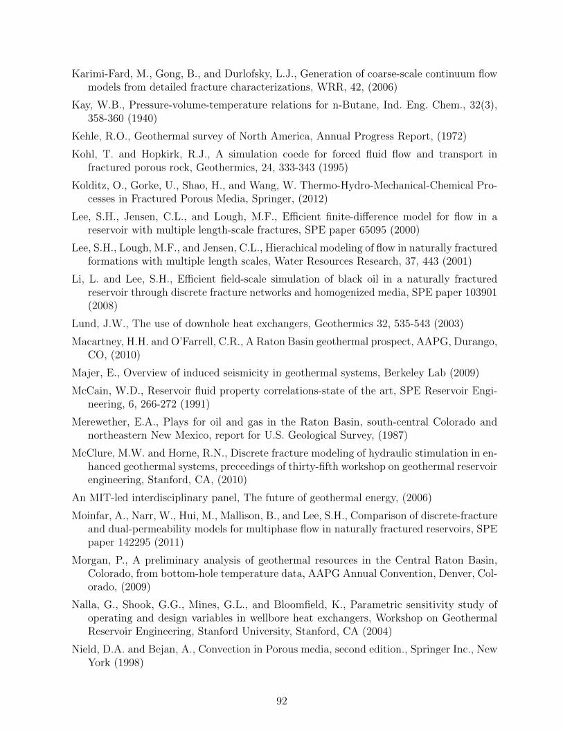
Karimi-Fard, M., Gong, B., and Durlofsky, L.J., Generation of coarse-scale continuum flowmodels from detailed fracture characterizations, WRR, 42, (2006)

Kay, W.B., Pressure-volume-temperature relations for n-Butane, Ind. Eng. Chem., 32(3),358-360 (1940)

Kehle, R.O., Geothermal survey of North America, Annual Progress Report, (1972)

Kohl, T. and Hopkirk, R.J., A simulation coede for forced fluid flow and transport infractured porous rock, Geothermics, 24, 333-343 (1995)

Kolditz, O., Gorke, U., Shao, H., and Wang, W. Thermo-Hydro-Mechanical-Chemical Pro-cesses in Fractured Porous Media, Springer, (2012)

Lee, S.H., Jensen, C.L., and Lough, M.F., Efficient finite-difference model for flow in areservoir with multiple length-scale fractures, SPE paper 65095 (2000)

Lee, S.H., Lough, M.F., and Jensen, C.L., Hierachical modeling of flow in naturally fracturedformations with multiple length scales, Water Resources Research, 37, 443 (2001)

Li, L. and Lee, S.H., Efficient field-scale simulation of black oil in a naturally fracturedreservoir through discrete fracture networks and homogenized media, SPE paper 103901(2008)

Lund, J.W., The use of downhole heat exchangers, Geothermics 32, 535-543 (2003)

Macartney, H.H. and O’Farrell, C.R., A Raton Basin geothermal prospect, AAPG, Durango,CO, (2010)

Majer, E., Overview of induced seismicity in geothermal systems, Berkeley Lab (2009)

McCain, W.D., Reservoir fluid property correlations-state of the art, SPE Reservoir Engi-neering, 6, 266-272 (1991)

Merewether, E.A., Plays for oil and gas in the Raton Basin, south-central Colorado andnortheastern New Mexico, report for U.S. Geological Survey, (1987)

McClure, M.W. and Horne, R.N., Discrete fracture modeling of hydraulic stimulation in en-hanced geothermal systems, preceedings of thirty-fifth workshop on geothermal reservoirengineering, Stanford, CA, (2010)

An MIT-led interdisciplinary panel, The future of geothermal energy, (2006)

Moinfar, A., Narr, W., Hui, M., Mallison, B., and Lee, S.H., Comparison of discrete-fractureand dual-permeability models for multiphase flow in naturally fractured reservoirs, SPEpaper 142295 (2011)

Morgan, P., A preliminary analysis of geothermal resources in the Central Raton Basin,Colorado, from bottom-hole temperature data, AAPG Annual Convention, Denver, Col-orado, (2009)

Nalla, G., Shook, G.G., Mines, G.L., and Bloomfield, K., Parametric sensitivity study ofoperating and design variables in wellbore heat exchangers, Workshop on GeothermalReservoir Engineering, Stanford University, Stanford, CA (2004)

Nield, D.A. and Bejan, A., Convection in Porous media, second edition., Springer Inc., NewYork (1998)

92

Patankar, S.V. and Spalding, D.B., A calculation procedure for heat, mass and momentumtransfer in three-dimensional parabolic flows, Int. J. Heat and Mass Transfer (1972)

Patankar, S.V., Numerical Heat Transfer and Fluid Flow, Hemisphere Publishing Corpo-ration, New York (1980)

Peaceman, D.W., Interpretation of well-block pressures in numerical reservoir simulation,SPE J., 18 (3), 183-194 (1978)

Plaksina, T., Modeling effects of coupled convection and CO2 injection in stimulating geo-pressured geothermal reservoirs, a Master’s thesis submitted to the graduate faculty ofLouisiana State University (2011).

Pritchett, J.W., STAR: A geothermal reservoir simulation system, Proceedings: WorldGeothermal Congress, Florence, (1995)

Pruess, K. and Narasimhan, T.N., A preactical method for modeling fluid and heat flow ina fractured porous media, SPE J., 25, 14-26 (1985)

Pruess, K. and Wang, J.S.Y., Numerical modeling of isothermal and nonisothermal flow inunsaturated fractured rock: a review, AGU, Special Symposium on Flow and Transportthrough Unsaturated Fractured Rocks, San Francisco, CA, (1986)

Pruess, K., Wang, J.S.Y., and Tsang, Y.W., On thermohyrological conditions near high-level nuclear wastes emplaced in partially saturated fractured tuff. Part 1. Simulationstudies with explicit consideration of fracture effects, Water Resources Research, 26,1235-1248 (1990)

Pruess, K., Wang, J.S.Y., and Tsang, Y.W., On thermohyrological conditions near high-level nuclear wastes emplaced in partially saturated fractured tuff. Part 2. Effectivecontinuum approximation, Water Resources Res., 26, 1249-1261 (1990)

Pruess, K., Oldenburg, C., and Moridis, G., TOUGH2 user’s guide, version 2.0, EarthSciences Division, Lawrence Berkeley National Laboratory, CA (2011)

Ray, C., Boast, C.W., Ellsworth, T.R., and Valocchi, A.J., Simulation of the impact ofagricultural management practices on chemical transport in macroporous soils, Tans. ofthe ASCE., 39(5), 1697-1707 (1996)

Rhie, C.M. and Chow, W.L., A numerical study of the turbulent flow past an isolatedairfold with trailing edge separation, AIAA Journal 21 1525-1532 (1983))

Rossen, R.H., Simulation of naturally fractured reservoir with semi-implicit source terms,SPEJ, (1977)

Rowe, A.M. and Chou, J.C.S., Pressure-volume-temperature-concentration relation of aque-ous NaCl solutions, Journal of Chemical Engineering Data, 15, (1970)

Rybach, L., How Renewable are geothermal resources?, Geothermal Resources CouncilTrans., Vol. 23, 563-566, (1999)

Rybach, L., Geothermal sustainability, GHC Bulletin, (2007)

Sanyal, S.K., Butler, S.J., Swenson, D., and Hardeman, B., Review of the state-of-the-art ofnumerical simulation of enhanced geothermal systems, Proceedings of World GeothermalCongress, Tohoku, Japan, (2000)

93

Sathiyamoorthy, M., Basak, T., Roy, S., and Pop, I., Steady natural convection flow in asquare cavity filled with a porous medium for linearly heated side wall(s), InternationalJournal of Heat and Mass Trans., 50, 1892-1901 (2007)

Svensson, U., A continuum representation of fracture networks. Part I: Method and basictest cases, journal of Hydrology, 250, 170-186 (2001)

Sybach, L., Megel, T., and Eugster, W.J., How renewable are geothermal resources?,Geothermal Resources Council Transactions, Vol. 23, 563-566 (1999)

Szalkowski, S.D. and Hanor, J.S., Spatial variations in the Salinity of produced waters fromsouthwstern Louisiana, GCAGS/GCSSEPM Trans., Vol. 53, 798-806 (2003)

Tester, J.W. and Albright, J.N., Hot dry rock energy extraction field test: first 75 daysof operation of a prototype reservoir at Fenton Hill, Los Alamos Scientific LaboratoryReport, (1979)

Thomas, L.K., Dixon, T., and Pierson, R.G., Fractured reservoir simulation, SPEJ, 42-54(1983)

Touma, J., Comparison of different capillary models to predict the hydraulic conductivityfrom the water retention curve, ISCO (2008)

U.S. DOE, Renewable energy technology characterizations, EERE (EPRI Topical ReportNo. TR-109496), (2005)

U.S. DOE, An evaluation of enhanced geothermal systems technology, EERE (2008)

Wang, Z., McClure M.W., and Horne, R.N., A single-well EGS configuration using a ther-mosiphon, Workshop on Geothermal Reservoir Engineering, Stanford University, Stan-ford, CA (2009)

Warren, J.E. and Root, P.J., The behavior of naturally fractured reservoirs, Soc. Petrol.Eng. J., 3, 245-255 (1963)

White, D.F. and Williams, D.L., Assessment of geothermal resources of the United States,U.S. Geological Survey Circular 726, (1975)

Witherspoon, P.A, Wang, J.S., Iwai, K., and Gale, E., Validity of cubic law for fluid flowin a deformable rock fracture, Water Resources Res., 16, 1016-1024 (1980)

Yamamoto, T., Kitano, K., Fujimitsu, Y., and Ohnishi, H., Application of simulation code,GEOTH3D, on the Ogachi HDR site, Proceedings of the 22rd Annual Workshop onGeothermal Reservoir Engineering, Stanford University, (1997)

94

Appendix A: Simulator Capabilities

Waterfooding Model

In the waterflooding case, the test results are demonstrated by comparing our blackoil sim-

ulator results against the Buckley-Leverett analytical solution. The relevant parameters are

listed in Table A.1. Figure A.1 shows a satisfactory comparison between computed results

and the analytical solution.

Table A.1: Parameters used for the waterflooding model.Sor 0.2 µo 1 cpSwc 0.2 µw 1 cpm 2 A 300 ft2

n 2 L 1000 ftφ 0.2 qt 100 stb/days

Figure A.1: Comparison of computed results against Buckley-Leverett analytical solution forwater saturation after 40 days.

95

Gravity & Capillary Effect

This case study verifies the gravity and capillary force balance calculations in a vertical 1-D

2-Phase system. The water saturation in the system initially distributes evenly at 0.5 (half

water and half air). Assuming a negligible compressibility, the water-air interface should be

stable at half of the total depth due to equilibrium. Figure A.2 and Figure A.3 present the

simulation results of water saturation at different grid resolutions and times. Table A.2 states

the Pc-Sw relation. Using Table A.2 as input, when the system reaches equilibrium, the water

saturation distribution should match the data from Table A.2, and Figure A.4 indicates the

excellent simulation results.

Figure A.2: Gravity induced water saturation distributions after 2 days and 20 days for thegrid resolution of ∆x=0.025ft.

96

Figure A.3: Gravity induced water saturation for different grid resolutions.

Table A.2: Pc-Sw relation (Touma, 2008).Sw Pc0.06 1.450.07 1.160.075 1.0150.08 0.870.09 0.580.1 0.435

0.3875 0.290.642 0.21750.974 0.1450.983 0.0725

97

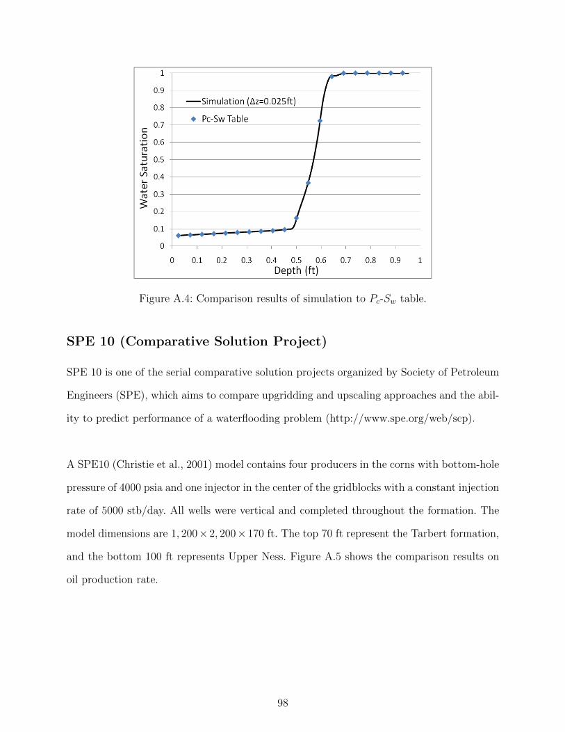
Figure A.4: Comparison results of simulation to Pc-Sw table.

SPE 10 (Comparative Solution Project)

SPE 10 is one of the serial comparative solution projects organized by Society of Petroleum

Engineers (SPE), which aims to compare upgridding and upscaling approaches and the abil-

ity to predict performance of a waterflooding problem (http://www.spe.org/web/scp).

A SPE10 (Christie et al., 2001) model contains four producers in the corns with bottom-hole

pressure of 4000 psia and one injector in the center of the gridblocks with a constant injection

rate of 5000 stb/day. All wells were vertical and completed throughout the formation. The

model dimensions are 1, 200× 2, 200× 170 ft. The top 70 ft represent the Tarbert formation,

and the bottom 100 ft represents Upper Ness. Figure A.5 shows the comparison results on

oil production rate.

98

Figure A.5: Comparing oil production rates with other simulation results (Christie et al.,2001).

Parallel Performance

The following tests were conducted to show the parallel performance of the code and two

types of scaling tests were conducted.

a) Strong scaling

A Strong scaling is used to show the ability of parallel computation to decrease the over all

run time for a particular problem. This test was carried out on a supercomputer, Queenbee,

over LONI resources, using 32, 64, 128, 256 and 512 cores and problem size is kept fixed at

4.8 × 106 gridblocks. Figure A.6 shows the result of strong scaling performance on log-log

plot.

99

Figure A.6: Log-log plot to strong scaling performance.

b) Weak scaling

A weak scaling test is used to show the ability of parallel computation scale up a problem

on more cores. Consequently, problem complexity is increased while increasing the number

of cores. Table A.3 indicates the number of gridblocks for its corresponding number of cores

and Figure A.7 presents the result of weak scaling performance on a log-log plot.

Table A.3: Computational cores vs. problem size.Number of Cores Gridblocks (∗103)

32 150128 600512 24001024 48002048 9600

100

Figure A.7: Log-log plot for weak scaling performance.

101

Appendix B: Discretization of TransportEquation

Eq. (B.1) presents a generalized form of transport equation which can stand for both fluid

flow and heat transfer equations.

ρ∂φ

∂t+ ρ(∇ · uφ)− µ∇2φ = Sφ (B.1)

where, ρ is the fluid density, φ is general variable and u stands for velocity vector. There

are four terms in above equation, from left to right, they are: transient term, convec-

tion/advection term, diffusion term and source term, respectively. By droping convection

term, flowing equation can be expressed. To represent energy transport, scalar variable tem-

perature is used as general variable, and for Navier-Stokes Equations, the source term is

represented as −∇P .

Finite Volume Discretization

Similar to the finite difference method for porous media, finite volume method is used to

evaluate partial differential equations in the form of algebraic equations for fracture, based

on which, values can be calculated at discrete places on a meshed geometry. However, one

advantage of the finite volume method over finite difference method is that it supports un-

structured mesh.

The governing equation for the flow in an arbitrary volume ∆V bounded by a closed surface

∆S can be described by taking integration of Navier-Stoke’s Equation.

∂

∂t

∫∆V

ρφ dV +

∫∆V

(ρ(∇ · uφ)− µ∇2φ) dV = −∫

∆V

Sφ dV (B.2)

By applying the divergence theorem in above equation, we have:

102

∂

∂t

∫∆V

ρφ dV +

∫∆S

ρuφ dS −∫

∆S

µ∇φ dS = −∫

∆V

Sφ dV (B.3)

where dS is the surface vector.

The transient and source therms are integrated over the cell volume, whereas, the con-

vection and diffusion therms sum the fluxes through the control volume faces.

Transient term

∂

∂t

∫∆V

ρφ dV = ρ∆VCφn+1C − φnC

∆t(B.4)

where, the subscript C represents the cell centroid.

Convection term

∫∆S

ρuφ dS =

∫∆S

ρufφf · nf dAf =∑f

Ffφf (B.5)

where, subscript f means cell face, n is normal vector, A represents face area and F is the

mass flux.

Diffusion term

−∫

∆S

µ∇φ dS = −∑f

µAf (∇φ)f · nf (B.6)

Source term

In the Navier-Stoke’s Equation, the source term or pressure gradient term can be approxi-

mated by Green-Gauss theorem which states that the volume integral of the gradient of the

103

scalar function is equal to the surface integral of a scalar function.

−∫

∆V

∇P dV = −∫

∆S

P dS = −∑f

P n+1f Afnf (B.7)

Otherwise, the source term can be simply estimated as:∫∆V

SφdV = Sφ∆V (B.8)

Interpolation Schemes

From above discretization, a lot variables on surface which need to be evaluated by variables

on other computational nodes. Thus, several interpolation schemes are introduced, although

only upwind scheme is employed in this study.

Upwind Differencing Scheme (UDS)

Upwind scheme approximates variable at surface using the value at the node upstream. Tech-

nically, it uses a backward or forward difference approximation on the basis of flow direction.

This scheme can not yield oscillation numerical diffusion will occur.

Taking Eq. (B.5) for example, using UDS, we have:

Ffuf =

Ffunb if Ff < 0

FfuC if Ff > 0(B.9)

Taylor series expansion gives:

uf = uC + (xf − xC)

(∂u

∂x

)C

+(xf − xC)2

2

(∂2u

∂x2

)C

+H (B.10)

where, H denotes higher-order terms.

From above equation, we can see UDS is a first order scheme and the leading truncation

error term(∂u∂x

)C

is diffusive.

104

Central Difference Scheme (CDS)

CDS approximates variable at surface by linear interpolation between two neighbor nodes.

For Eq. (B.5), we have:

uf = (1− λ)uC + λunb (B.11)

where, λ is the weigh coefficient which can be defined asxf−xCxnb−xC

.

Taylor series expansion gives:

uf = unbλ+ uC(1− λ)− (xf − xC)(xnb − xf )2

(∂2u

∂x2

)C

+H (B.12)

The CDS is a simple second order scheme and may produce oscillatory solutions. The lead-

ing truncation error term is proportional to the square of the grid spacing. According to the

nature of convection, the one more point required is on the upstream side.

Quadratic Upstream Interpolation for Convective Kinematics (QUICK)

Leonard (1979) made this scheme popular and named it as QUICK which approximates

variables by a parabola instead of a straight line. The general form of QUICK scheme is

shown as following expressions.

φe =

g1φE − g2φW + (1− g1 + g2)φP for ux < 0

g3φP − g4φEE + (1− g3 + g4)φE for ux > 0(B.13)

where,

g1 =(2− λe,W )λ2

e,P

1 + λe,P − λe,W(B.14)

g2 =(1− λe,P )(1− λe,W )2

1 + λe,P − λe,W(B.15)

g3 =(1 + λe,W )(1− λe,P )2

1 + λe,E − λe,P(B.16)

105

g4 =λe,Pλ

2e,E

1 + λe,E − λe,P(B.17)

For uniform grid with ux > 0, the coefficients can be calculated and the Taylor series expan-

sion gives:

φe =6

8φP +

3

8φE −

1

8φW −

3(∆x)3

48

(∂3φ

∂x3

)P

+H (B.18)

The above expression indicates the QUICK scheme has a third order truncation error. How-

ever, the overall approximation will still be the second order accuracy when this scheme is

used with midpoint rule approximation of surface intergral.

Navier-Stokes Equations Solver

This section presents the solution to the Navier-Stokes euqations with Re=1000. SIMPLE

(Semi-Implicit Method for Pressure-Linked Equations) algorithm, developed by Spalding

and Patankar (1972), is used for pressure-velocity coupling. The momentum interpolation

presented by Rhie and Chow (1983) is employed for calculating the cell-face mass fluxes to

avoid the pressure oscillation. The boundary condition of driven cavity system is shown in

Figure B.1, Figure B.2 and Figure B.3 are the simulation results compared to the results

presented by Ghia et al. (1982).

The solution procedures are summarized as followings.

1. Guess pressure field and flux.

2. Solve velocities on the basis of assumed pressure field and flux.

3. Calculate coefficients for pressure correlation and assemble coefficient matrix.

4. Solve the discretized pressure correlation equation.

5. Correct pressure, velocities and fluxes.

106

6. Calculate temperature field and update related properties.

7. Repeat steps 2-6.

Figure B.1: Boundary condition of driven cavity system.

Figure B.2: U velocity profile at x=0.5.

107

Figure B.3: V velocity profile at y=0.5.

The coupling of Navier-Stokes equations with porous media flow is defined as a further work.

108

Appendix C: User’s Manual

Simulator Installation

The presented geothermal simulator is built based upon the Cactus framework which is de-

signed for developing portable, modular applications. A Cactus code consists of a core part

”Flesh” and a set of modules called ”thorns”. The Flesh works as a utility and service library

providing thorns with information or action. In contrast, thorns are the modules contain-

ing different functionalities. Several steps can be follow to build up the geothermal simulator.

Getting the Code

One way to download Cactus is to use the ”GetComponents” script which takes an argument

the name of a file containing a ThornList. The script is available at:

https://raw.github.com/gridaphobe/CRL/ET 2011 10/GetComponents

Alternatively, svn is also applicable to check out Cactus. The main Cactus Subversion Server

(svn.cactuscode.org) hosts several different repositories including different branches for the

stable and development versions of Cactus. Check out the Cactus flesh:

svn co http://svn.cactuscode.org/flesh/trunk Cactus

Configuring

The purpose of configuration is to determine compilers and compilation ags suitable for the

current architecture. The general command is shown as:

gmake <config name>-config <option name>=<chosen value> , ...

Since the presented geothermal simulator includes several external softwares (OpenMPI,

HDF5, PETSc and ParMetis), the full configuration command using in this study is:

109

gmake thermal-config LIB=parmetis, HDF5=yes, MPI=OpenMPI, PETSC=yes

However, Cactus cannot setup or locate the installed external softwares. Before running con-

figuration command, the softwares should be installed properly, and all the corresponding

environmental variables (PATH, LD LIBRARY PATH, LIBDIRS, PETSC DIR, HDF5 DIR,

OPENMPI DIR, PETSC ARCH) have to be specified, for example

export PETSC ARCH=”linux-gnu-c”.

Compiling

Once the new configuration (”thermal”) has been successfully created, the corresponding

executable can be built using following command:

gmake thernal SILENT=no

The default executable will be stored in the folder called ”./exe” with the default name of

”cactus thermal”. ”SILENT=no” is a compilation option to make the compiler output more

details during compiling.

Running

Cactus executables always run from a parameter le which species which thorns to use and

sets the values of each thorns parameters. The command line used in this study is:

cactus thermal thermal.par

The name of parameter file is ”thermal.par”, although there is no restriction on it. A pa-

rameter le is a text le whose lines are either comments (begin with ’#’ or ’ !’) or parameter

statements (parameter names followed by an ’=’, followed by the value for these parameters).

The first parameter statement in any parameter file is ActiveThorns, which is a special

110

parameter that tells the program which thorns are to be activated. And only parameters

from active thorns can be set, since all thorns are set to be inactive by default.

Example: Saturated Geothermal Reservoirs

To run a case which can achieve the same result as shown in Figure 4.12, several thorns need

to be checked out first and the thornlist is as follows.

CactusBase/Boundary

CactusBase/CartGrid3D

CactusBase/CoordBase

CactusBase/IOASCII

CactusBase/IOBasic

CactusBase/IOUtil

CactusBase/LocalInterp

CactusBase/LocalReduce

CactusBase/SymBase

CactusBase/Time

CactusConnect/HTTPD

CactusConnect/HTTPDExtra

CactusConnect/Socket

CactusExternal/FlexIO

CactusExternal/jpeg6b

CactusIO/IOJpeg

CactusPUGH/PUGH

CactusPUGH/PUGHInterp

CactusPUGH/PUGHReduce

CactusPUGH/PUGHSlab

CactusPUGHIO/IOHDF5

111

CactusPUGHIO/IOHDF5Util

CactusUtils/NaNChecker

CactusUtils/TimerReport

ResSim/BlackOilBase

ResSim/BlackOilEvolve

ResSim/GeoThermal

ResSim/IDBlackOil

ResSimExamples/GeoT

Sandbox/LocalToGlobal

where, BlackOilBase, IDBlackOil contain variable definitions and data initialization; Black-

OilEvolve and Geothermal thorns solve mass and heat transport equations, respectively.

The parameter file is attached as follows to demonstrate how to setup the above prob-

lem.

ActiveThorns=”geot localtoglobal coordbase cartgrid3d pugh blackoilbase blackoilevolve geother-

mal idblackoil boundary symbase timerreport ioascii iobasic ioutil pughslab iohdf5 iohdf5util

httpd httpdextra socket iojpeg localreduce pughreduce Time”

cactus::terminate = ”time”

cactus::cctk final time = 13000

cactus::cctk timer output = ”full”

Time::timestep method = ”given”

Time::timestep = 5

driver::global nx=57

driver::global ny=57

driver::global nz=37

driver::ghost size=1

driver::padding active = ”no”

112

driver::enable all storage = ”yes”

# domain size

grid::domain = ”full”

grid::type =”coordbase”

coordbase::xmin= 0

coordbase::xmax= 6679.3

coordbase::ymin= 0

coordbase::ymax= 6679.3

coordbase::zmin= 0

coordbase::zmax= 472.3

coordbase::ncells x=56

coordbase::ncells y=56

coordbase::ncells z=36

coordbase::spacing=”numcells”

Above statements describe the simulation setting include simulation time, domain size,

timestep, mesh generation and etc.

# setting up IDblackoil parameters

idblackoil::InitializePressureFromOWC = ”no”

idblackoil::DefaultPorosity = 0.2

idblackoil::DefaultPermXX = 200

idblackoil::DefaultPermYY = 200

idblackoil::DefaultPermZZ = 200

idblackoil::DefaultPw = 13200

blackoilbase::DipAngleX=5

blackoilbase::DipAngleY=5

geothermal::TGrad=0.0154

113

geothermal::Tsur=275.6

geothermal::DHE Length=2624

geothermal::DHE Reinjection=3280

geothermal::DHE I=44

geothermal::DHE J=44

geothermal::DHE K=25

geothermal::DHE Projection I=-0.706665

geothermal::DHE Projection J=-0.706665

geothermal::DHE Projection K=-0.035333

Geothermal reservoir properties are setup, including dip angle along x and y axis (Di-

pAngleX and DipAngleY), thermal gradient (TGrad), temperature at top surface (Tsur).

DHE configurations are also covered: length, reinjection distance, DHE starting point in

reservoir (DHE I, DHE J, DHE K), and direction vector along x, y, z (DHE Projection I,

DHE Projection J, DHE Projection K).

# setting up solver

BlackOilEvolve::absTol = 1e-8

BlackOilEvolve::relTol = 1e-9

BlackOilEvolve::imp tolerance = 1e-8

BlackOilEvolve::max imp counter = 800

BlackOilEvolve::BlackOilStepKSPType = ”bcgs”

BlackOilEvolve::BOPCType = ”bjacobi”

Convergence tolerance, linear equation solver and preconditioner are specified as above.

# setup output

IO::out mode = ”onefile”

IO::out unchunked = ”yes”

114

IO::out dir = ”Geothermal”

IOBASIC::outScalar criterion = ”iteration”

IOBasic::outInfo every = 1

IOBasic::outInfo vars = ”BlackOilBase::Pw BlackOilBase::Tt”

iohdf5::out every = 6

iohdf5::out dir = ”Geothermal”

iohdf5::out vars = ”blackoilbase::Pw blackoilbase::Tt”

Screen and HDF5 output options are selected.

115

Vita

Yin Feng was born in December, 1981, in Daqing, Heilongjiang, China. He finished his un-

dergraduate studies at Dalian University of Technology, Dalian, in June 2004. He earned

a master of science degree in petroleum engineering from the University of Louisiana at

Lafayette in December 2007. He is currently a candidate for the degree of Doctor of Philos-

ophy in petroleum engineering, to be awarded in August 2012.

116