Ozone loss and chlorine activation in the Arctic winters 1991-2003 derived with the tracer-tracer...
33
Atmos. Chem. Phys., 4, 2181–2213, 2004 www.atmos-chem-phys.org/acp/4/2181/ SRef-ID: 1680-7324/acp/2004-4-2181 Atmospheric Chemistry and Physics Ozone loss and chlorine activation in the Arctic winters 1991–2003 derived with the tracer-tracer correlations S. Tilmes 1 , R. M ¨ uller 1 , J.-U. Grooß 1 , and J. M. Russell III 2 1 Institute of Stratospheric Research (ICG-I), Forschungszentrum J¨ ulich, Germany 2 Hampton University, Hampton, Virginia 23668, USA Received: 11 March 2004 – Published in Atmos. Chem. Phys. Discuss.: 4 May 2004 Revised: 22 July 2004 – Accepted: 1 August 2004 – Published: 15 November 2004 Abstract. Chemical ozone loss in the Arctic stratosphere was investigated for the twelve years between 1991 and 2003 employing the ozone-tracer correlation method. For this method, the change in the relation between ozone and a long- lived tracer is considered for all twelve years over the lifetime of the polar vortex to calculate chemical ozone loss. Both the accumulated local ozone loss in the lower stratosphere and the column ozone loss were derived consistently, mainly on the basis of HALOE satellite observations. HALOE mea- surements do not cover the polar region homogeneously over the course of the winter. Thus, to derive an early winter ref- erence function for each of the twelve years, all available measurements were additionally used; for two winters cli- matological considerations were necessary. Moreover, a de- tailed quantification of uncertainties was performed. This study further demonstrates the interaction between meteo- rology and ozone loss. The connection between tempera- ture conditions and chlorine activation, and in turn, the con- nection between chlorine activation and ozone loss, becomes obvious in the HALOE HCl measurements. Additionally, the degree of homogeneity of ozone loss within the vortex was shown to depend on the meteorological conditions. Results derived here are in general agreement with the re- sults obtained by other methods for deducing polar ozone loss. Differences occur mainly owing to different time pe- riods considered in deriving accumulated ozone loss. How- ever, very strong ozone losses as deduced from SAOZ for January in winters 1993–1994 and 1995–1996 cannot be identified using available HALOE observations in the early winter. In general, strong accumulated ozone loss was found to occur in conjunction with a strong cold vortex containing a large volume of possible PSC existence (V PSC ), whereas moderate ozone loss was found if the vortex was less strong and moderately warm. Hardly any ozone loss was calculated Correspondence to: S. Tilmes ([email protected]) for very warm winters with small amounts of V PSC during the entire winter. This study supports the linear relationship between V PSC and the accumulated ozone loss reported by Rex et al. (2004) if V PSC was averaged over the entire win- ter period. Here, further meteorological factors controlling ozone loss were additionally identified if V PSC was averaged over the same time interval as that for which the accumu- lated ozone loss was deduced. A significant difference in ozone loss (of ≈36 DU) was found due to the different dura- tion of solar illumination of the polar vortex of at maximum 4 hours per day in the observed years. Further, the increased burden of aerosols in the atmosphere after the Pinatubo vol- canic eruption in 1991 significantly increased the extent of chemical ozone loss. 1 Introduction The mixing ratio of stratospheric ozone in the Arctic vortex is determined by both chemical reactions and by transport. In particular, the most prominent transport process inside the polar vortex is the diabatic descent of air during winter. De- scent of air tends to increase the ozone mixing ratio at a given altitude, because ozone mixing ratios increase with altitudes in the lower stratosphere. Thus, air with large mixing ra- tios of ozone is transported downwards into the lower strato- sphere, the region where chemical ozone destruction occurs. Ozone variations due to transport are often of the same mag- nitude as those due to chemical ozone destruction (e.g. Man- ney et al., 1994; von der Gathen et al., 1995; M¨ uller et al., 1996; Rex et al., 2003a). Therefore, it is necessary to sep- arate these two processes in order to quantify the chemical ozone loss in the stratosphere. Different approaches have been developed over the past decade to separate transport and chemistry employing the ex- plicit model calculation of diabatic descent (e.g. Rex et al., 1999b; Manney et al., 2003a; Knudsen et al., 1998; Goutail © European Geosciences Union 2004
-
Upload
independent -
Category
Documents
-
view
1 -
download
0
Transcript of Ozone loss and chlorine activation in the Arctic winters 1991-2003 derived with the tracer-tracer...

Atmos. Chem. Phys., 4, 2181–2213, 2004www.atmos-chem-phys.org/acp/4/2181/SRef-ID: 1680-7324/acp/2004-4-2181
AtmosphericChemistry
and Physics
Ozone loss and chlorine activation in the Arctic winters 1991–2003derived with the tracer-tracer correlations
S. Tilmes1, R. Muller1, J.-U. Grooß1, and J. M. Russell III2
1Institute of Stratospheric Research (ICG-I), Forschungszentrum Julich, Germany2Hampton University, Hampton, Virginia 23668, USA
Received: 11 March 2004 – Published in Atmos. Chem. Phys. Discuss.: 4 May 2004Revised: 22 July 2004 – Accepted: 1 August 2004 – Published: 15 November 2004
Abstract. Chemical ozone loss in the Arctic stratospherewas investigated for the twelve years between 1991 and 2003employing the ozone-tracer correlation method. For thismethod, the change in the relation between ozone and a long-lived tracer is considered for all twelve years over the lifetimeof the polar vortex to calculate chemical ozone loss. Boththe accumulated local ozone loss in the lower stratosphereand the column ozone loss were derived consistently, mainlyon the basis of HALOE satellite observations. HALOE mea-surements do not cover the polar region homogeneously overthe course of the winter. Thus, to derive an early winter ref-erence function for each of the twelve years, all availablemeasurements were additionally used; for two winters cli-matological considerations were necessary. Moreover, a de-tailed quantification of uncertainties was performed. Thisstudy further demonstrates the interaction between meteo-rology and ozone loss. The connection between tempera-ture conditions and chlorine activation, and in turn, the con-nection between chlorine activation and ozone loss, becomesobvious in the HALOE HCl measurements. Additionally, thedegree of homogeneity of ozone loss within the vortex wasshown to depend on the meteorological conditions.
Results derived here are in general agreement with the re-sults obtained by other methods for deducing polar ozoneloss. Differences occur mainly owing to different time pe-riods considered in deriving accumulated ozone loss. How-ever, very strong ozone losses as deduced from SAOZ forJanuary in winters 1993–1994 and 1995–1996 cannot beidentified using available HALOE observations in the earlywinter. In general, strong accumulated ozone loss was foundto occur in conjunction with a strong cold vortex containinga large volume of possible PSC existence (VPSC), whereasmoderate ozone loss was found if the vortex was less strongand moderately warm. Hardly any ozone loss was calculated
Correspondence to:S. Tilmes([email protected])
for very warm winters with small amounts of VPSC duringthe entire winter. This study supports the linear relationshipbetween VPSC and the accumulated ozone loss reported byRex et al. (2004) if VPSC was averaged over the entire win-ter period. Here, further meteorological factors controllingozone loss were additionally identified if VPSCwas averagedover the same time interval as that for which the accumu-lated ozone loss was deduced. A significant difference inozone loss (of≈36 DU) was found due to the different dura-tion of solar illumination of the polar vortex of at maximum4 hours per day in the observed years. Further, the increasedburden of aerosols in the atmosphere after the Pinatubo vol-canic eruption in 1991 significantly increased the extent ofchemical ozone loss.
1 Introduction
The mixing ratio of stratospheric ozone in the Arctic vortexis determined by both chemical reactions and by transport.In particular, the most prominent transport process inside thepolar vortex is the diabatic descent of air during winter. De-scent of air tends to increase the ozone mixing ratio at a givenaltitude, because ozone mixing ratios increase with altitudesin the lower stratosphere. Thus, air with large mixing ra-tios of ozone is transported downwards into the lower strato-sphere, the region where chemical ozone destruction occurs.Ozone variations due to transport are often of the same mag-nitude as those due to chemical ozone destruction (e.g. Man-ney et al., 1994; von der Gathen et al., 1995; Muller et al.,1996; Rex et al., 2003a). Therefore, it is necessary to sep-arate these two processes in order to quantify the chemicalozone loss in the stratosphere.
Different approaches have been developed over the pastdecade to separate transport and chemistry employing the ex-plicit model calculation of diabatic descent (e.g. Rex et al.,1999b; Manney et al., 2003a; Knudsen et al., 1998; Goutail
© European Geosciences Union 2004

2182 S. Tilmes et al.: Ozone loss and chlorine activation in the Arctic winters 1991–2003
et al., 1999; Lefevre et al., 1998; Harris et al., 2002). An-other possibility of deriving chemical ozone loss is to excludetransport processes implicitly by the tracer-tracer correlationmethod (e.g. Proffitt et al., 1990; Muller et al., 1996, 1999,2002; Tilmes et al., 2003b), as is used in this study.
Chemical ozone loss in the polar stratosphere is caused be-yond doubt by the burden of CFCs in the atmosphere, whichis due to anthropogenic emissions (e.g. Solomon, 1999;WMO, 2003). The inactive chlorine reservoir species areconverted into an active – ozone-destroying – form throughheterogeneous reactions on the surface of polar stratosphericclouds (PSCs). PSCs form during a cold period of the Arc-tic winter. Therefore, chemical ozone depletion is linked tometeorological conditions (e.g. Manney et al., 2003a; Rexet al., 2004). Santee et al. (2003) discussed the connectionbetween interannual variability of the ClO abundance andmeteorological conditions during the 1990s. The strongestClO abundance was found in the very cold winter of 1995–1996 in the Arctic lower stratosphere.
In this paper, ozone loss was analysed consistently over theperiod of the last twelve years (1991–1992 to 2002–2003) us-ing the tracer-tracer correlation method, mainly on the basisof Version 19 HALOE satellite observations (Russell et al.,1993). Recent improvements to the method (Muller et al.,2002; Tilmes et al., 2003b) and further enhancements, de-scribed in this study, allow a comprehensive error analysis ofthe derived chemical ozone loss. We present a detailed anal-ysis for each year including the correlation between ozoneloss, chlorine activation and the volume of possible PSC ex-istence (VPSC).
A comparison is made between ozone loss derived usingthe tracer-tracer correlation method and other methods us-ing model simulations to estimate transport processes. Reli-able results within the range of uncertainty during a periodof twelve years allow us to consider the correlation betweenVPSCand the calculated column ozone loss and accumulatedlocal ozone loss between early winter and spring. The cor-relation indicates an increase of ozone loss with increasingVPSC. This relation is not a linear correlation if the sametime interval of ozone loss calculations and VPSC averagingis considered. Besides VPSC, here further dependences of thechemical ozone loss were found. Other factors control chem-ical ozone loss. The illumination time of solar radiation ontocold parts of the vortex may have significant influence onozone loss, as well as the loading of volcanic sulfate aerosolsin the atmosphere.
2 The tracer-tracer correlation technique
2.1 Methodology
The TRAcer-tracer Correlation technique (referred to as“TRAC technique” in the following) has its origins in thestudy by Roach (1962) and later Allam et al. (1981). They
first noticed that a relation between two different speciesarises through the elimination of dynamical variability frommeasurements in the atmosphere. Compact relations be-tween long-lived tracers in the stratosphere were first ob-served by Ehhalt et al. (1983) and were simulated usingvarious chemical transport models (Mahlman et al., 1986;Holton, 1986; Plumb and Ko, 1992; Avallone and Prather,1997) and recently by Sankey and Shepherd (2003). Proffittet al. (1990) first developed the TRAC technique to quantifychemical ozone loss inside an isolated vortex from high al-titude aircraft measurements. Later this technique was ap-plied and extended to satellite (Muller et al., 1996, 1997;Tilmes et al., 2003b) and balloon (Muller et al., 2001; Salaw-itch et al., 2002) measurements. The TRAC method wasfurther used to investigate chlorine activation (through theanalysis of HCl-tracer correlations) (e.g. Muller et al., 1996;Tilmes et al., 2003a) and denitrification (through the analysisof NOy-N2O correlations) (e.g. Fahey et al., 1996; Rex et al.,1999a).
Over the course of the winter, constant compact relation-ships are expected for tracers with sufficiently long lifetimesfor the air mass inside a polar vortex that is largely iso-lated from the surrounding air masses (Plumb and Ko, 1992).Therefore, advection in the polar vortex, in particular dia-batic decent, cannot alter the relation between two chemi-cally long-lived tracers (e.g. Proffitt et al., 1992; Proffitt et al.,1993). If one of the tracers is subject to chemical or physicalchange (active tracer), owing to the particular meteorologicalconditions inside the polar vortex, changes in mixing ratioare identified as changes of the tracer-tracer correlation (e.g.Proffitt et al., 1992; Muller et al., 1996, 2002; Tilmes et al.,2003b).
Here, we use the TRAC method to consider the correla-tion of two long-lived tracers inside the polar vortex dur-ing twelve Arctic winter periods. To decide whether profilesare inside or outside the Arctic vortex a methodology is em-ployed based on UKMO meteorological analyses allowingaccurate selection criteria (Tilmes et al., 2003b). Three vor-tex regions are defined, based on the algorithm derived byNash et al. (1996), the vortex core, the outer vortex (the areabetween vortex core and vortex edge) and the outer part of thevortex boundary region (outside the vortex edge). Further,trajectory calculations were used to reposition each measuredprofile to noon. This is the time at which UKMO meteoro-logical analyses are available to apply the Nash et al. (1996)algorithm .
The HALOE instrument (Russell et al., 1993) measurestwo long-lived tracers, namely CH4 and HF. Both tracers canbe used individually to calculate chemical ozone loss with theTRAC technique because their lifetimes are sufficiently long(Muller et al., 2002; Tilmes et al., 2003b). Additionally, theuse of these two long-lived tracers enables a further improvedselection criterion for the HALOE profiles. Because CH4and HF have very long lifetimes, the relationship betweenCH4 and HF inside the polar vortex region is nearly linear
Atmos. Chem. Phys., 4, 2181–2213, 2004 www.atmos-chem-phys.org/acp/4/2181/

S. Tilmes et al.: Ozone loss and chlorine activation in the Arctic winters 1991–2003 2183
Table 1. CH4/HF reference relations from HALOE observations inside the vortex core: 1991–1992 to 2002–2003. Polynomial functionsof the form: [y]=
∑ni =0 ai ·[x]
i with n≤4 are shown as well as the standard deviation of the observation points from the fitted referencefunctionσ .
valid [x] a0 a1 a2 a3 a4 σ
1991–19920.1–1.1 1.83 −2.49 2.72 −3.31 1.63 9.03×10⁻²
1992–19930.1–1.3 1.64 −1.71 7.33×10⁻¹
−1.91×10⁻²−1.55×10⁻¹ 9.95×10⁻²
1993–19940.1–1.35 1.85 −2.75 3.70 −3.15 9.31×10⁻¹ 1.04×10⁻¹
1994–19950.1–1.4 1.76 −2.71 4.18 −3.71 1.10 8.98×10⁻²
1995–19960.1–1.5 1.65 −1.16 1.77×10⁻¹
−3.63×10⁻² 8.11×10⁻²
1996–19970.1–1.5 1.76 −1.88 2.25 −2.00 5.87×10⁻¹ 7.92×10⁻²
1997–19980.1–1.55 1.71 −1.47 8.75×10⁻¹
−4.91×10⁻¹ 8.44×10⁻² 8.14×10⁻²
1998–19990.2–1.6 1.98 −3.44 4.84 −3.40 8.07×10⁻¹ 8.46×10⁻²
1999–20000.1–1.65 1.72 −1.89 1.53 −8.55×10⁻¹ 1.73×10⁻¹ 8.67×10⁻²
2000–20010.1–1.7 2.05 −2.99 4.10 −3.05 7.54×10⁻¹ 7.27×10⁻²
2001–20020.1–1.6 1.89 −2.54 2.90 −1.93 4.40×10⁻¹ 7.39×10⁻²
2002–20030.1–1.6 1.91 −2.93 3.90 −2.66 0.61 8.75×10⁻²
and does not change significantly over the whole lifetime ofthe vortex in each year. In this study, a linear relationshipof HALOE measurements was derived from profiles insidethe polar vortex for each year, with a standard deviation ofless than 0.1 ppmv (Table 1). Profiles deviating by more than0.2 ppmv from the constant CH4/HF relation are neglectedin order to eliminate observations that are uncertain.
Besides CH4 and HF, the HALOE instrument measuresozone and HCl, which are used as the active tracers in thisstudy. HCl is chemically destroyed by heterogeneous reac-tions and increases due to the deactivation of chlorine via thereaction of Cl with CH4. Chemical ozone loss occurs if largeconcentrations of chemically active halogen compounds arepresent in an air mass. This is the case in most years in latewinter and spring inside the polar vortex in the presence ofsunlight.
To derive chemical losses of ozone, first the ozone-tracerrelation has to be determined at a time before ozone haschemically changed. This is usually the case in the earlywinter when rather little sunlight is present. The ozone-tracer relation, referred to as “early winter reference func-tion”, is mathematically formulated as a polynomial and isconsidered as the reference for chemically unperturbed con-
ditions. It is necessary to derive an early winter referencefunction for each of the twelve years considered to deter-mine chemical ozone loss for each year. The observationtime of the underlying profiles considered has to be cho-sen carefully for this purpose. The turning point from sum-mer to winter circulation marks the time of the formationof the polar vortex. Thus, the time of the minimum of theozone column density is the earliest time at which the earlywinter reference function can be determined. This point intime can be derived considering the total ozone column fromglobal satellite measurements. Tilmes (2003, Sect. 3.3) usedTOMS observations for this purpose. On the other hand, thistime of the winter may not be the most suitable time to de-rive the early winter reference function if the early vortex isnot yet strong enough. Horizontal mixing across the vortexedge may change the tracer-tracer relation without chemicalchanges. A case in point is the winter 1996–1997, wherethe ozone-tracer relation changed until the beginning of Jan-uary 1997, due to horizontal mixing processes (Tilmes et al.,2003b). Further, in winter 1991–1992 the ozone-tracer rela-tion changed from November 1991 to December 1991 due tomixing (see Sect. 3.1).
www.atmos-chem-phys.org/acp/4/2181/ Atmos. Chem. Phys., 4, 2181–2213, 2004

2184 S. Tilmes et al.: Ozone loss and chlorine activation in the Arctic winters 1991–2003
In summary, the early winter reference function has to bedetermined at a time when the vortex has already formed and,additionally, is sufficiently isolated from mid-latitude air, butat the same time early enough so that no ozone loss has yettaken place. Therefore, if the vortex is isolated, the referencefunction has to be derived as early as possible, if observa-tions are available. These conditions are generally fulfilledfor each of the derived reference functions and some excep-tions will be discussed in detail below.
To draw conclusions on possible chlorine activation andtherefore possible ozone loss in a certain time period, theconsideration of the value of “volume of possible PSC exis-tence”, VPSC, is useful because significant chlorine activationis not possible without the existence of PSCs (e.g. Solomon,1999). Additionally, here, the amount of solar illuminationon the cold parts of the polar vortex is considered. Signifi-cant ozone loss is not possible without the existence of ac-tive chlorine components and further, without the presenceof sunlight (e.g. Solomon, 1999).
VPSCdescribes the total volume on a certain potential tem-perature level, where the temperature (here determined fromthe UKMO analysis) does not exceed the PSC threshold tem-perature. This PSC threshold temperature was calculated(Hanson and Mauersberger, 1988) for a HNO3 mixing ra-tio of 10 ppbv and a H2O mixing ratio of 5 ppmv. There-fore, if PSC existence is not possible at the time before theearly winter reference function was derived, no chlorine ac-tivation and thus no ozone loss should have occurred. On theother hand, an existing potential for PSCs during the earlywinter may result in active chlorine components that causeozone loss if sunlight is present (see below). Using VPSCas an indicator for chlorine activation, one has to keep inmind that these calculations of VPSC do not include PSCswhich occur on the mesoscale due to orographically inducedmountain waves (e.g. Fueglistaler et al., 2003). Further, theuse of different meteorological analyses may result in differ-ences up to≈25% of temperature analyses (Knudsen et al.,2002; Manney et al., 2003a) and therefore in differences inthe calculated VPSC. If HALOE measurements are availableat the time for which the early winter reference function isdetermined, chlorine activation can be clearly detected fromthe TRAC analysis of HCl-tracer correlations (Muller et al.,1996; Tilmes et al., 2003a) as a strong loss of HCl.
HALOE makes measurements fifteen times per day ateach sunrise and sunset occultation along two latitude lines.These lines move between 80◦ N and 80◦ S in about 45 days.Therefore, measurements in high northern latitudes are avail-able every two or three months, depending on the year andin most of the years considered relatively few observationswere available inside the early vortex. Thus, to derive theearly winter reference function, additional data sources suchas ILAS satellite measurements and balloon measurementswere used.
For two out of twelve winters, for which no direct mea-surements could be obtained in the early vortex, a methodol-
ogy has been developed to estimate the early winter referencefunctions. In this way, for each of the twelve winters con-sidered a reliable early winter O3-tracer reference functioncould be derived, as described below in Sect. 3.
A reliable calculation of ozone loss during the course ofthe winter is possible, as long as the polar vortex is iso-lated well enough so that the tracer-tracer correlation remainscompact and unaltered in the absence of chemical changes.Tilmes et al. (2003b) and Tilmes (2003) have shown that acompact ozone-tracer correlation exists inside the polar vor-tex during January in the Arctic winter 1996–1997 when nochemical ozone loss is expected due to the lack of sunlightbased on ILAS observations. The ILAS instrument measuredseven months in high northern latitudes (58◦ N–73◦ N), thusproviding good coverage of the polar vortex over this timeperiod. Moreover, it was shown that the vortex has to beisolated well enough to obtain a compact reliable referencecorrelation. In the winter 1996–1997 this situation was foundfor the Arctic vortex since early January 1997. Further, dur-ing winter and spring an exact criterion has to be defined todecide whether profiles are measured in or outside the vortex,because the characteristics of air outside the vortex are verydifferent to vortex air. Using a mixture of profiles measuredin and outside the vortex will lead to the erroneous conclu-sion that a compact ozone-tracer correlation does not exist.
Khosrawi et al. (2004) discussed the evolution of O3/N2Oof different isentropic levels based on ILAS measurements1996–97. They did not separate isentropic levels at differ-ent altitudes into measurements inside and outside the vortexand therefore did not obtain a compact January relationship,whereas exactly the same data indicate a compact O3/N2Ocorrelation inside the vortex core if sorted according to thevortex criterion used here (Tilmes, 2003) (Fig. 4.4, the pole-ward edge of the vortex boundary region, using the algorithmderived by Nash et al., 1996).
In the study by Sankey and Shepherd (2003), the O3/CH4correlation is considered in the course of an Arctic winteranalysing results of the CMAM model. The ozone-tracer cor-relations from the model on the different isentropic levels aresimilar to those derived by Khosrawi et al. (2004) based onILAS observations. Thus the shape of the lines should not beseen as a lack of compactness inside the polar vortex, as it isinterpreted by Sankey and Shepherd (2003), but it is ratherthe result of considering measurements in high northern lati-tudes, which are not separated into profiles measured outsideand inside the polar vortex.
Further, Muller et al. (2001) used balloon-borne measure-ments in the Arctic winter 1991–1992 to show that the im-pact of mixing between air masses from outside the vor-tex with air inside the vortex would result in a tendency togreater ozone mixing ratios in the ozone-tracer relation. Re-cent model calculations for the development of tracer distri-butions in the winter 1999/2000 (Konopka et al., 2003) cor-roborate this finding. The effect should thus lead to an under-estimation of the chemical ozone loss. Tilmes et al. (2003b),
Atmos. Chem. Phys., 4, 2181–2213, 2004 www.atmos-chem-phys.org/acp/4/2181/

S. Tilmes et al.: Ozone loss and chlorine activation in the Arctic winters 1991–2003 2185
using ILAS observations for winter 1996–1997, have shownthat this effect is not significant after early January 1997.Even inside the vortex remnants in May 1997, a compact cor-relation is found.
In this study we argue that a compact correlation existsduring all the observed twelve Arctic winters. Especially,the analysis of the very warm winters (1998–1999 and 2001–2002) – where no substantial chemical ozone loss is expected– demonstrates that the ozone-tracer correlations do not sig-nificantly change due to mixing processes, although the vor-tices are less strong compared to other winters. Only if thevortex completely breaks down and reforms, as was the casein March 2001, is it impossible to obtain reliable results us-ing the TRAC technique.
2.2 Error analysis
An error analysis was performed consistently for all the yearsanalysed here. In the early winter and during the course ofthe winter, the scatter of the ozone-tracer relations arises, onthe one hand, due to variability of the mixing ratios of tracersinside the vortex, and, on the other hand, it may possibly bedue to the random error of the satellite measurements. Boththese uncertainties are estimated by calculating the standarddeviation of the profiles contributing to the early winter ref-erence function.
Further, no systematic error of the satellite measurementsis taken into account because assuming that all availablemeasurements of one satellite are affected in the same way itwould have no impact on the ozone loss calculation. There-fore, the uncertainty of results was derived from the uncer-tainty of the early winter reference function. Additionally,the standard deviation of monthly averaged column ozoneloss deduced from the individual profiles is considered. Thisdescribes the homogeneity of the deduced ozone loss duringa particular time span and in a particular region. Inhomo-geneities may be caused by both the inhomogeneity of theozone loss inside the vortex and the random error of the satel-lite measurements, as described above.
Mixing processes may change the early winter referencefunction without chemical change if the vortex is not iso-lated. However, a significant increase in the uncertaintyrange due to mixing processes in the early vortex is not ex-pected, because each profile used to derive an early win-ter reference function was located poleward of the vortexedge (using the Nash criterion). The vortex was isolated formost years considered at the time when the reference func-tion was derived. This can be assumed regarding the evo-lution of calculated PV values at the vortex edge using theNash criterion. At the time when the reference function wasderived, PV values at the vortex edge are 30–35 PV units(1PVU=10−6 K m2/(kg s)) at the 475 K level for all year. Inthe following two weeks, PV values increase in the most ofthe years at the 475 K level (except for the winter 1998–1999). Therefore, the uncertainty due to dynamics on the
reference function should be small in all the years consid-ered. In 1998–1999 the vortex was less strong although stillisolated; in this winter, a stronger influence of mixing on theearly vortex reference cannot be excluded.
The impact of mixing processes during the entire winterperiod of the years considered should be small for the samereason. Only in the middle of February 2001 did the vortexbreak down completely. Therefore, no ozone loss is calcu-lated after this event. In 1991–1992, a major warming at theend of January may have impacted the tracer-tracer correla-tions leading to an underestimation of chemical ozone lossin this year (see Sect. 2.1). Therefore, the derived value ofozone loss for this winter constitutes a lower limit. Further,results of the winter 1997–1998 and 2000–2001 had to be de-rived using a reference function based on climatology valuesand are thus more uncertain compared to results derived froma reference function based directly on measurements of thespecific year. Nevertheless, these reference functions are theaverage of all the de-trended early winter reference functionsand should therefore be reliable within the reported range ofuncertainty.
To derive results with minimum uncertainty, it is alsonecessary to calculate ozone loss in the appropriate altituderange. Column ozone loss is therefore calculated for an al-titude range of 380–550 K, 400–500 K and 40–100 hPa (tocompare the results with other studies) from HALOE obser-vations, because within this range the empirical ozone-tracerreference relations are valid and possible mixing processesbelow 380 K are excluded. The smallest uncertainty arisesif the column ozone loss is calculated in an altitude rangebetween 400–500 K. Here, the vortex is most compact andaccuracies of satellite data are better than at lower altitudes.
3 Impact of meteorological conditions on ozone-tracerand HCl-tracer relations
3.1 Development of early winter reference functions
The early winter reference function is derived individuallyfrom all available HALOE measurements inside the earlyvortex for the six winters 1992–1993 to 1995–1996 and in1998–1999 and 2001–2002. The profiles used were locatedinside the early vortex for each year, at a time when in generalno ozone loss was expected (as outlined below). For 1991–1992 (Muller et al., 2001), 1999–2000 (Muller et al., 2002)and 2002–2003 (Tilmes et al., 2003a), early winter referencefunctions were derived from balloon observations. In winter1996–1997, ILAS observations were used to define an earlywinter reference function to calculate ozone loss from mea-surements made by HALOE in late winter and spring (Tilmeset al., 2003b).
An overview of the mathematically formulated tracer-tracer early winter reference functions derived only fromHALOE observations inside the early vortex is summarised
www.atmos-chem-phys.org/acp/4/2181/ Atmos. Chem. Phys., 4, 2181–2213, 2004
2186 S. Tilmes et al.: Ozone loss and chlorine activation in the Arctic winters 1991–2003
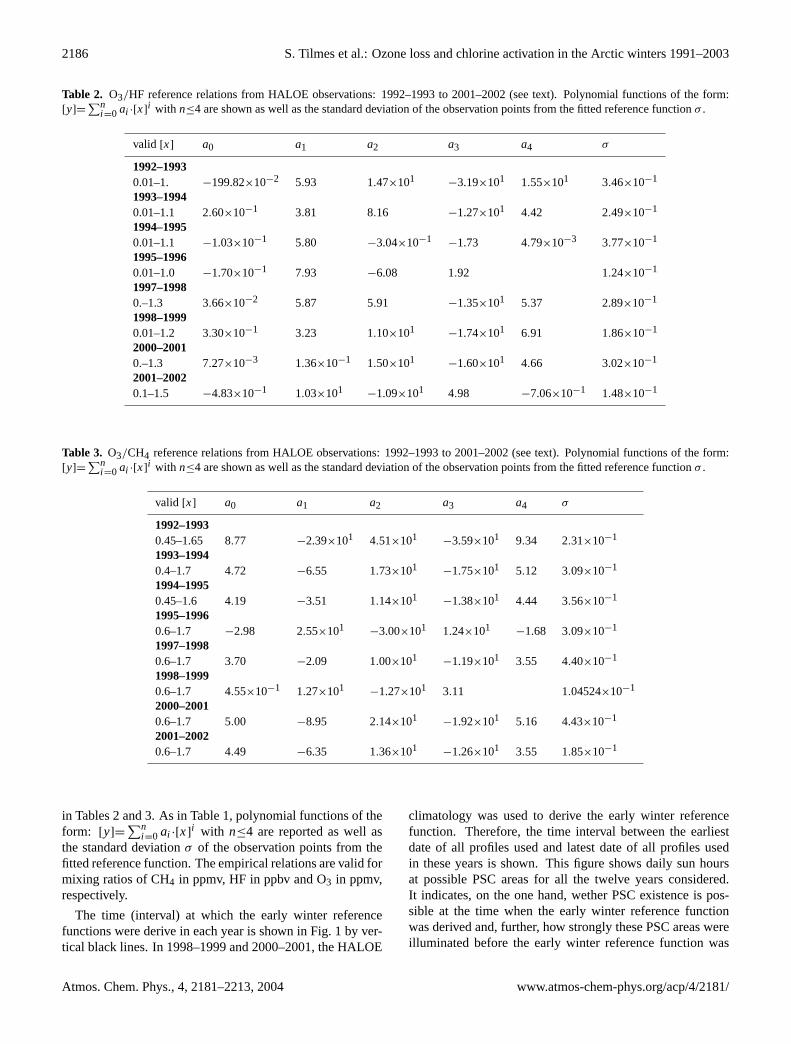
Table 2. O3/HF reference relations from HALOE observations: 1992–1993 to 2001–2002 (see text). Polynomial functions of the form:[y]=
∑ni =0 ai ·[x]
i with n≤4 are shown as well as the standard deviation of the observation points from the fitted reference functionσ .
valid [x] a0 a1 a2 a3 a4 σ
1992–19930.01–1. −199.82×10⁻² 5.93 1.47×101
−3.19×101 1.55×101 3.46×10⁻¹
1993–19940.01–1.1 2.60×10⁻¹ 3.81 8.16 −1.27×101 4.42 2.49×10⁻¹
1994–19950.01–1.1 −1.03×10⁻¹ 5.80 −3.04×10⁻¹
−1.73 4.79×10⁻³ 3.77×10⁻¹
1995–19960.01–1.0 −1.70×10⁻¹ 7.93 −6.08 1.92 1.24×10⁻¹
1997–19980.–1.3 3.66×10⁻² 5.87 5.91 −1.35×101 5.37 2.89×10⁻¹
1998–19990.01–1.2 3.30×10⁻¹ 3.23 1.10×101
−1.74×101 6.91 1.86×10⁻¹
2000–20010.–1.3 7.27×10⁻³ 1.36×10⁻¹ 1.50×101
−1.60×101 4.66 3.02×10⁻¹
2001–20020.1–1.5 −4.83×10⁻¹ 1.03×101
−1.09×101 4.98 −7.06×10⁻¹ 1.48×10⁻¹
Table 3. O3/CH4 reference relations from HALOE observations: 1992–1993 to 2001–2002 (see text). Polynomial functions of the form:[y]=
∑ni =0 ai ·[x]
i with n≤4 are shown as well as the standard deviation of the observation points from the fitted reference functionσ .
valid [x] a0 a1 a2 a3 a4 σ
1992–19930.45–1.65 8.77 −2.39×101 4.51×101
−3.59×101 9.34 2.31×10⁻¹
1993–19940.4–1.7 4.72 −6.55 1.73×101
−1.75×101 5.12 3.09×10⁻¹
1994–19950.45–1.6 4.19 −3.51 1.14×101
−1.38×101 4.44 3.56×10⁻¹
1995–19960.6–1.7 −2.98 2.55×101
−3.00×101 1.24×101−1.68 3.09×10⁻¹
1997–19980.6–1.7 3.70 −2.09 1.00×101
−1.19×101 3.55 4.40×10⁻¹
1998–19990.6–1.7 4.55×10⁻¹ 1.27×101
−1.27×101 3.11 1.04524×10⁻¹
2000–20010.6–1.7 5.00 −8.95 2.14×101
−1.92×101 5.16 4.43×10⁻¹
2001–20020.6–1.7 4.49 −6.35 1.36×101
−1.26×101 3.55 1.85×10⁻¹
in Tables 2 and 3. As in Table 1, polynomial functions of theform: [y]=
∑ni =0 ai ·[x]
i with n≤4 are reported as well asthe standard deviationσ of the observation points from thefitted reference function. The empirical relations are valid formixing ratios of CH4 in ppmv, HF in ppbv and O3 in ppmv,respectively.
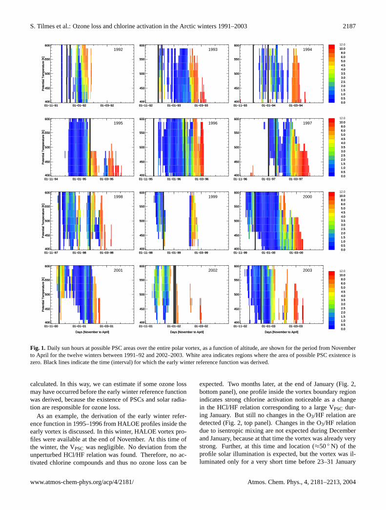
The time (interval) at which the early winter referencefunctions were derive in each year is shown in Fig. 1 by ver-tical black lines. In 1998–1999 and 2000–2001, the HALOE
climatology was used to derive the early winter referencefunction. Therefore, the time interval between the earliestdate of all profiles used and latest date of all profiles usedin these years is shown. This figure shows daily sun hoursat possible PSC areas for all the twelve years considered.It indicates, on the one hand, wether PSC existence is pos-sible at the time when the early winter reference functionwas derived and, further, how strongly these PSC areas wereilluminated before the early winter reference function was
Atmos. Chem. Phys., 4, 2181–2213, 2004 www.atmos-chem-phys.org/acp/4/2181/
S. Tilmes et al.: Ozone loss and chlorine activation in the Arctic winters 1991–2003 2187
400
450
500
550
600P
oten
tial T
empe
ratu
re [K
]
400
450
500
550
600P
oten
tial T
empe
ratu
re [K
]
01−11−91 01−01−92 01−03−92
01−11−91 01−01−92 01−03−92
1992
400
450
500
550
600
400
450
500
550
600
01−11−92 01−01−93 01−03−93
01−11−92 01−01−93 01−03−93
1993
400
450
500
550
600
400
450
500
550
600
01−11−93 01−01−94 01−03−94
01−11−93 01−01−94 01−03−94
1994
0.00.51.01.52.02.53.03.54.04.55.06.08.0
10.0
0.00.51.01.52.02.53.03.54.04.55.06.08.0
10.0 12.0
400
450
500
550
600
Pot
entia
l Tem
pera
ture
[K]
400
450
500
550
600
Pot
entia
l Tem
pera
ture
[K]
01−11−94 01−01−95 01−03−95
01−11−94 01−01−95 01−03−95
1995
400
450
500
550
600
400
450
500
550
600
01−11−95 01−01−96 01−03−96
01−11−95 01−01−96 01−03−96
1996
400
450
500
550
600
400
450
500
550
600
01−11−96 01−01−97 01−03−97
01−11−96 01−01−97 01−03−97
1997
0.00.51.01.52.02.53.03.54.04.55.06.08.0
10.0
0.00.51.01.52.02.53.03.54.04.55.06.08.0
10.0 12.0
400
450
500
550
600
Pot
entia
l Tem
pera
ture
[K]
400
450
500
550
600
Pot
entia
l Tem
pera
ture
[K]
01−11−97 01−01−98 01−03−98
01−11−97 01−01−98 01−03−98
1998
400
450
500
550
600
400
450
500
550
600
01−11−98 01−01−99 01−03−99
01−11−98 01−01−99 01−03−99
1999
400
450
500
550
600
400
450
500
550
600
01−11−99 01−01−00 01−03−00
01−11−99 01−01−00 01−03−00
2000
0.00.51.01.52.02.53.03.54.04.55.06.08.0
10.0
0.00.51.01.52.02.53.03.54.04.55.06.08.0
10.0 12.0
400
450
500
550
600
Pot
entia
l Tem
pera
ture
[K]
400
450
500
550
600
Pot
entia
l Tem
pera
ture
[K]
01−11−00 01−01−01 01−03−01
Days [November to April]
01−11−00 01−01−01 01−03−01
Days [November to April]
2001
400
450
500
550
600
400
450
500
550
600
01−11−01 01−01−02 01−03−02
Days [November to April]
01−11−01 01−01−02 01−03−02
Days [November to April]
2002
400
450
500
550
600
400
450
500
550
600
01−11−02 01−01−03 01−03−03
Days [November to April]
01−11−02 01−01−03 01−03−03
Days [November to April]
2003
0.00.51.01.52.02.53.03.54.04.55.06.08.0
10.0
0.00.51.01.52.02.53.03.54.04.55.06.08.0
10.0 12.0
Fig. 1. Daily sun hours at possible PSC areas over the entire polar vortex, as a function of altitude, are shown for the period from Novemberto April for the twelve winters between 1991–92 and 2002–2003. White area indicates regions where the area of possible PSC existence iszero. Black lines indicate the time (interval) for which the early winter reference function was derived.
calculated. In this way, we can estimate if some ozone lossmay have occurred before the early winter reference functionwas derived, because the existence of PSCs and solar radia-tion are responsible for ozone loss.
As an example, the derivation of the early winter refer-ence function in 1995–1996 from HALOE profiles inside theearly vortex is discussed. In this winter, HALOE vortex pro-files were available at the end of November. At this time ofthe winter, the VPSC was negligible. No deviation from theunperturbed HCl/HF relation was found. Therefore, no ac-tivated chlorine compounds and thus no ozone loss can be
expected. Two months later, at the end of January (Fig. 2,bottom panel), one profile inside the vortex boundary regionindicates strong chlorine activation noticeable as a changein the HCl/HF relation corresponding to a large VPSC dur-ing January. But still no changes in the O3/HF relation aredetected (Fig. 2, top panel). Changes in the O3/HF relationdue to isentropic mixing are not expected during Decemberand January, because at that time the vortex was already verystrong. Further, at this time and location (≈50◦ N) of theprofile solar illumination is expected, but the vortex was il-luminated only for a very short time before 23–31 January
www.atmos-chem-phys.org/acp/4/2181/ Atmos. Chem. Phys., 4, 2181–2213, 2004

2188 S. Tilmes et al.: Ozone loss and chlorine activation in the Arctic winters 1991–2003
0.0 0.2 0.4 0.6 0.8 1.0 1.2
HF (ppbv)
0
1
2
3
4
O3
(ppm
v)
18.−23.11.95 23.−31.1.96
0.0 0.2 0.4 0.6 0.8 1.0 1.2
HF (ppbv)
0.0
0.5
1.0
1.5
2.0
2.5
3.0
HC
l (pp
bv)
18.−23.11.95 23.−31.1.96
Fig. 2. Tracer-tracer profiles inside the outer early vortex of theyear 1995–1996 from HALOE measurements with HF as the pas-sive tracer. In the top panel, the chemical active tracer is O3 and inthe bottom panel the chemical active tracer is HCl. The early winterreference function for the O3/HF relation 1995–1996, top panel, isindicated as a black solid line and the uncertainty of the referencefunction is represented by black dotted lines.
1996 (see Fig. 1). Therefore, the HCl was already stronglyreduced although little ozone loss inside the range of uncer-tainty of the reference function was found. Of course, theHCl-tracer relation changes much faster than the O3-tracerrelation, because chlorine activation occurs on much shortertime scales than ozone loss. The fact that in 1996 – in spiteof the early vortex having been cold and strong – no signifi-cant ozone loss occurred during January may be explained bythe very small amount of sunlight that illuminated the earlyvortex.
In the following, the derivation of the early winter ref-erence function from balloon observations in 1991–1992,1999–2000 and 2002–2003 is briefly described. Thereafter,early winter reference functions of the other years consideredare discussed. For winter 1991–1992, the early winter refer-ence function was derived from measurements of ozone andN2O made by cryosampler measurements (Schmidt et al.,1987) on 5 and 12 December 1991, respectively. At thistime, a small VPSC was calculated, but these VPSC are notilluminated (see Fig. 1) and therefore no ozone loss can beexpected before this time.
The O3/N2O profiles were transformed to O3/CH4 with theN2O/CH4 relationship from Engel et al. (1996), see Muller
6−Nov−1991 to 14−Jan−1992
0.4 0.6 0.8 1.0 1.2 1.4 1.6
CH4 (ppmv)
0
1
2
3
4
5
O3
(ppm
v)
Kiruna Balloons 5.12.91
Kiruna Balloons 12.12.91
Kiruna Balloons 5.12.91
Kiruna Balloons 12.12.91
Fig. 3. The early winter reference function 1991–1992, shown as ablack line, was derived from balloon measurements from December1991 (coloured symbols). Dotted lines indicate the range of uncer-tainty in the reference function. Observations made by HALOEwithin the vortex in November 1991 (black plus signs) and in Jan-uary (black squares) are also shown.
et al. (2001). To derive the O3/HF reference function, theO3/CH4 relation was converted using the CH4/HF relationderived from HALOE observations for the winter 1991–1992(Table 1).
The vortex started forming in November 1991. OneHALOE profile was found inside the early vortex at the be-ginning of November, with low ozone mixing ratios com-pared to profiles inside the vortex measured in January (seeFig. 3, black plus signs). At that time the vortex was notwell developed and mixing in of air masses from outside thevortex was still possible. Therefore, the low ozone mixingratios observed in November increased until the vortex be-came fully isolated in December. The HALOE profiles inJanuary 1992 scatter below the derived reference relation byabout 1.2 ppmv CH4 level (see Fig. 3). Thus ozone loss hadalready occurred during January 1992, in accordance witha relatively small, but illuminated volume of possible PSCexistence in the first two weeks of January (see Figs. 1 and8). In contrast to the winter 1995–1996, ozone loss duringJanuary 1992 was much stronger although VPSC in January1996 was even larger than in January 1991–1992. However,VPSCwere much less illuminated in January 1996 comparedto January 1992 (see Fig. 1). This shows that ozone loss isinfluenced by solar radiation in addition to VPSC, as furtherdiscussed in Sect. 6.
In winter 1999–2000, again no HALOE observations wereavailable inside the early vortex to derive the early winter ref-erence function. Fortunately, during the SOLVE-THESEO2000 campaign two balloon flights have been conducted in-side the early vortex, the OMS (Observations of the Middle
Atmos. Chem. Phys., 4, 2181–2213, 2004 www.atmos-chem-phys.org/acp/4/2181/
S. Tilmes et al.: Ozone loss and chlorine activation in the Arctic winters 1991–2003 2189
0.2 0.4 0.6 0.8 1.0 1.2
HF (ppbv)
0
1
2
3
4
5
O3
(ppm
v)
1991/1992 1992/1993 1993/1994 1994/1995 1995/1996 1996/1997 1998/1999 1999/2000 2001/2002 2002/2003
0.4 0.6 0.8 1.0 1.2 1.4 1.6
CH4 (ppmv)
0
1
2
3
4
5
O3
(ppm
v)
1991/1992 1992/1993 1993/1994 1994/1995 1995/1996 1996/1997 1998/1999 1999/2000 2001/2002 2002/2003
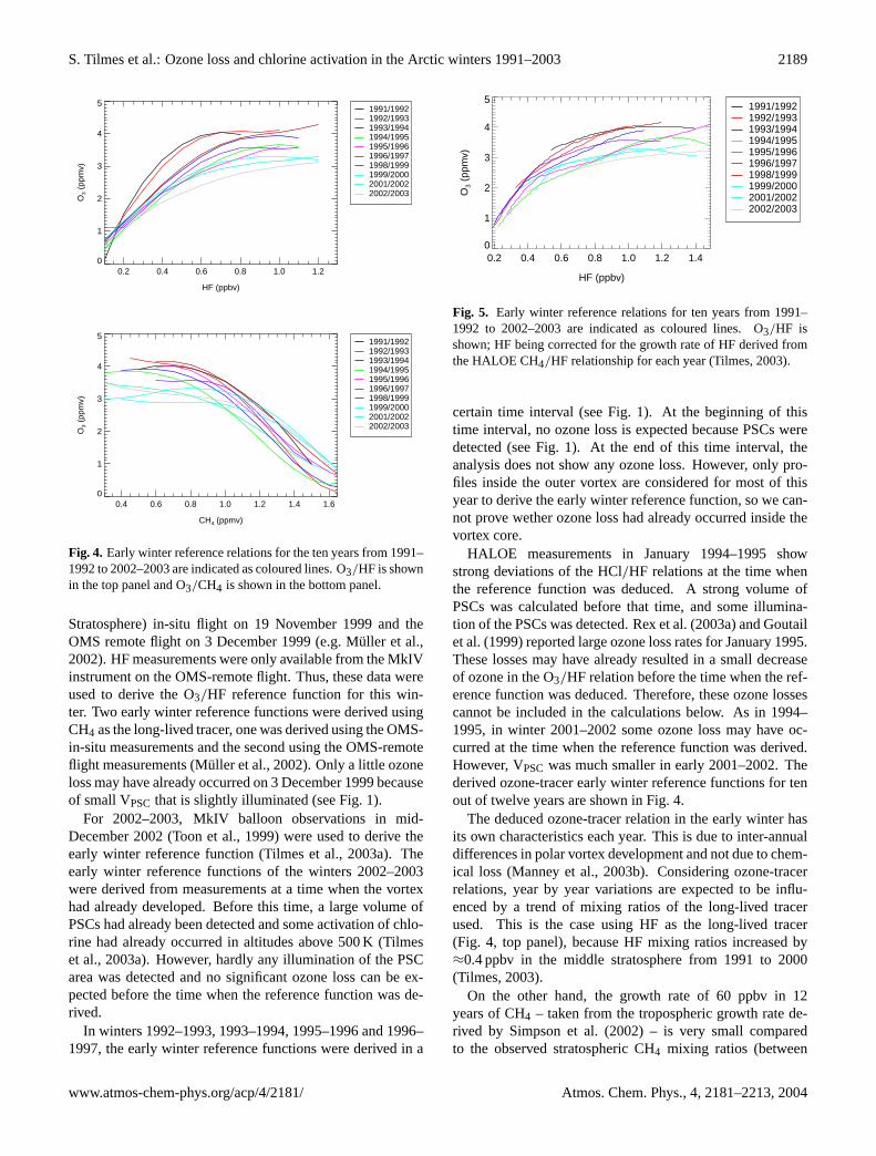
Fig. 4. Early winter reference relations for the ten years from 1991–1992 to 2002–2003 are indicated as coloured lines. O3/HF is shownin the top panel and O3/CH4 is shown in the bottom panel.
Stratosphere) in-situ flight on 19 November 1999 and theOMS remote flight on 3 December 1999 (e.g. Muller et al.,2002). HF measurements were only available from the MkIVinstrument on the OMS-remote flight. Thus, these data wereused to derive the O3/HF reference function for this win-ter. Two early winter reference functions were derived usingCH4 as the long-lived tracer, one was derived using the OMS-in-situ measurements and the second using the OMS-remoteflight measurements (Muller et al., 2002). Only a little ozoneloss may have already occurred on 3 December 1999 becauseof small VPSC that is slightly illuminated (see Fig. 1).
For 2002–2003, MkIV balloon observations in mid-December 2002 (Toon et al., 1999) were used to derive theearly winter reference function (Tilmes et al., 2003a). Theearly winter reference functions of the winters 2002–2003were derived from measurements at a time when the vortexhad already developed. Before this time, a large volume ofPSCs had already been detected and some activation of chlo-rine had already occurred in altitudes above 500 K (Tilmeset al., 2003a). However, hardly any illumination of the PSCarea was detected and no significant ozone loss can be ex-pected before the time when the reference function was de-rived.
In winters 1992–1993, 1993–1994, 1995–1996 and 1996–1997, the early winter reference functions were derived in a
0.2 0.4 0.6 0.8 1.0 1.2 1.4
HF (ppbv)
0
1
2
3
4
5
O3
(ppm
v)
1991/1992 1992/1993 1993/1994 1994/1995 1995/1996 1996/1997 1998/1999 1999/2000 2001/2002 2002/2003
Thu Jun 24 11:16:17 2004imone/IDL/HALOE_PRO/haloe_intern_set_plot.pro HF_SCATTER/haloe_hf_references_detr.ps
Fig. 5. Early winter reference relations for ten years from 1991–1992 to 2002–2003 are indicated as coloured lines. O3/HF isshown; HF being corrected for the growth rate of HF derived fromthe HALOE CH4/HF relationship for each year (Tilmes, 2003).
certain time interval (see Fig. 1). At the beginning of thistime interval, no ozone loss is expected because PSCs weredetected (see Fig. 1). At the end of this time interval, theanalysis does not show any ozone loss. However, only pro-files inside the outer vortex are considered for most of thisyear to derive the early winter reference function, so we can-not prove wether ozone loss had already occurred inside thevortex core.
HALOE measurements in January 1994–1995 showstrong deviations of the HCl/HF relations at the time whenthe reference function was deduced. A strong volume ofPSCs was calculated before that time, and some illumina-tion of the PSCs was detected. Rex et al. (2003a) and Goutailet al. (1999) reported large ozone loss rates for January 1995.These losses may have already resulted in a small decreaseof ozone in the O3/HF relation before the time when the ref-erence function was deduced. Therefore, these ozone lossescannot be included in the calculations below. As in 1994–1995, in winter 2001–2002 some ozone loss may have oc-curred at the time when the reference function was derived.However, VPSC was much smaller in early 2001–2002. Thederived ozone-tracer early winter reference functions for tenout of twelve years are shown in Fig. 4.
The deduced ozone-tracer relation in the early winter hasits own characteristics each year. This is due to inter-annualdifferences in polar vortex development and not due to chem-ical loss (Manney et al., 2003b). Considering ozone-tracerrelations, year by year variations are expected to be influ-enced by a trend of mixing ratios of the long-lived tracerused. This is the case using HF as the long-lived tracer(Fig. 4, top panel), because HF mixing ratios increased by≈0.4 ppbv in the middle stratosphere from 1991 to 2000(Tilmes, 2003).
On the other hand, the growth rate of 60 ppbv in 12years of CH4 – taken from the tropospheric growth rate de-rived by Simpson et al. (2002) – is very small comparedto the observed stratospheric CH4 mixing ratios (between
www.atmos-chem-phys.org/acp/4/2181/ Atmos. Chem. Phys., 4, 2181–2213, 2004

2190 S. Tilmes et al.: Ozone loss and chlorine activation in the Arctic winters 1991–2003
0.5–1.5 ppmv) and therefore is not significant for the presentanalysis. Further, ozone was relatively constant during the1990s in northern mid-latitudes (WMO, 2003). Neverthe-less, a decrease of ozone was found in the polar regions, butmainly in the southern hemisphere (WMO, 2003). Therefore,considering O3/CH4 reference functions (Fig. 4, bottompanel) the interannual differences of the early winter ref-erence functions are not a result of a significant trend ofmethane. In this study, we obtain some indications of a trendof ozone in high northern altitudes towards lower ozone mix-ing ratios, but interannual differences in ozone mixing ra-tios are possible for different reasons (as described below).O3/HF early winter reference functions can be de-trendedwith regard to HF, using the HF growth rate deduced fromthe HALOE HF/CH4 relationships (Table 1) (Tilmes, 2003).
The range of interannual differences of≈1 ppmv ozonemixing ratio – in altitudes above the 0.8 ppbv level of HFor the 1.0 ppmv level of CH4 – are similar for both O3/HFand O3/CH4 relationships (see Figs. 4, bottom panel and 5).The largest ozone mixing ratios are found in winter 1991–1992. This is possibly due to enhanced global transport inthis winter owing to the eruption of Pinatubo in June 1991.Very small ozone mixing ratios are found for the three win-ters 1999–2000, 2001–2002 and 2002–2003. This may bedue to an earlier isolation of the polar vortex, for examplein winter 2002–2003. Additionally, ozone loss may have al-ready occurred at the time when the reference function wasderived in winter 1999–2000 and 2001–2002 (see Fig. 1).Due to the different influences that control ozone mixing ra-tios in high northern latitudes in the early winter, a possibletrend of ozone cannot be determined in this study.
Thus, it is not possible to use one single reference functionfor all years. For the winter 1997–1998 and 2000–2001, nei-ther HALOE nor any other measurements were obtained inthe early vortex. Therefore, the early winter reference func-tions of these years were constructed from a climatology ofall HALOE profiles measured inside the early vortex overthe ten year period between 1992 and 2002. Actually, mea-surements inside the early vortex are available for six win-ters (1992–1993, 1993–1994, 1994–1995, 1995-1996, 1998–1999 and 2001–2002). The HALOE O3/HF and O3/CH4profiles are corrected for the growth rate of HF and CH4,respectively, between each single year and the year 1997–1998 (2000–2001). The CH4 growth was taken from thetropospheric growth rate (Simpson et al., 2002). The HFgrowth rate was deduced from the HALOE HF/CH4 rela-tionships (Table 1) (Tilmes, 2003). No correction was ap-plied to ozone, as described above. Thus, for winters 1997–1998 and 2000–2001 in each case two early winter referencerelations were derived, one using HF as the long-lived tracerand one using CH4 (Tables 2 and 3).
3.2 The evolution of tracer-tracer relations during twelveArctic winters
Active chlorine inside the polar vortex causes chemicalozone loss in the presence of sunlight. Chlorine activation inthe Arctic lower stratosphere may be identified as a strong re-duction of HCl compared to normal values. Therefore, usingmeasurements made by HALOE, the evolution of the chlo-rine chemistry can be inferred from the development of theHCl-tracer relation during each year. The evolution of HCl-tracer relation and O3-tracer relation is analysed for each ofthe twelve observed winter periods (Figs. 6 and 7). Lowtemperatures in the polar vortex cause the formation of PSCand thus control the activation of chlorine and consequentlythe chemical destruction of ozone. If temperatures are suffi-ciently low PSCs occur in the polar stratosphere. Therefore,VPSC is used here to analyse the interaction between mete-orological conditions and development of tracer-tracer rela-tionships for each winter (Fig. 8). Further, a division intocold, moderately cold and warm winters is carried out at theend of this section. Additionally, a measure of the strengthof the vortex is determined.
– 1991–1992:The cold vortex in winter 1991–1992 was disturbed byseveral warming pulses between November and Febru-ary (Naujokat et al., 1992). The threshold temperaturefor PSCs was only reached during January. Therefore,significant ozone depletion can be expected starting inJanuary 1992. At the end of January, a major warmingresulted in transport of air into the vortex (e.g. Grooßet al., 2003). However, the vortex in the lower strato-sphere was not much affected. The zonal winds at 60◦ Nconsiderably weakened, but remained westerly (Nau-jokat et al., 1992). In the second part of March and April1992, ozone loss was found to be homogeneous in theArctic vortex. This is an indication that the air fromoutside that entered the vortex at the end of Januarywas well mixed within the vortex during March andApril. During March, the temperatures at the North Polesteadily increased and the vortex finally broke down atthe end of April (Naujokat et al., 1992). In January,February and at the beginning of March, very low HClmixing ratios are clearly noticeable and strong chlorineactivation (Fig. 6) occurred in the lower stratosphere.HCl mixing ratios are nearly zero in January and lessthan 0.3 ppbv in February below the 0.6 ppbv HF level,which is below the 420 K potential temperature level.
By April, the HCl levels increased towards unperturbedvalues, especially at altitudes below≈420 K. The vortexbecame steadily weaker during April. From Februaryup to the beginning of April a moderate homogeneousdeviation from O3/HF reference functions occurred.
Atmos. Chem. Phys., 4, 2181–2213, 2004 www.atmos-chem-phys.org/acp/4/2181/

S. Tilmes et al.: Ozone loss and chlorine activation in the Arctic winters 1991–2003 2191
HALOE 91−92
0.0 0.2 0.4 0.6 0.8 1.0 1.2 1.40.0
0.5
1.0
1.5
2.0
2.5
HC
l (pp
bv)
HALOE 92−93
0.0 0.2 0.4 0.6 0.8 1.0 1.2 1.40.0
0.5
1.0
1.5
2.0
2.5HALOE 93−94
0.0 0.2 0.4 0.6 0.8 1.0 1.2 1.40.0
0.5
1.0
1.5
2.0
2.5
HALOE 94−95
0.0 0.2 0.4 0.6 0.8 1.0 1.2 1.40.0
0.5
1.0
1.5
2.0
2.5
HC
l (pp
bv)
HALOE 95−96
0.0 0.2 0.4 0.6 0.8 1.0 1.2 1.40.0
0.5
1.0
1.5
2.0
2.5HALOE 96−97
0.0 0.2 0.4 0.6 0.8 1.0 1.2 1.40.0
0.5
1.0
1.5
2.0
2.5
HALOE 97−98
0.0 0.2 0.4 0.6 0.8 1.0 1.2 1.40.0
0.5
1.0
1.5
2.0
2.5
HC
l (pp
bv)
HALOE 98−99
0.0 0.2 0.4 0.6 0.8 1.0 1.2 1.40.0
0.5
1.0
1.5
2.0
2.5HALOE 99−00
0.0 0.2 0.4 0.6 0.8 1.0 1.2 1.40.0
0.5
1.0
1.5
2.0
2.5
HALOE 00−01
0.0 0.2 0.4 0.6 0.8 1.0 1.2 1.4
HF (ppbv)
0.0
0.5
1.0
1.5
2.0
2.5
HC
l (pp
bv)
HALOE 01−02
0.0 0.2 0.4 0.6 0.8 1.0 1.2 1.4
HF (ppbv)
0.0
0.5
1.0
1.5
2.0
2.5HALOE 02−03
0.0 0.2 0.4 0.6 0.8 1.0 1.2 1.4
HF (ppbv)
0.0
0.5
1.0
1.5
2.0
2.5
Fig. 6. HCl/HF relations are shown for the twelve winters between 1991–1992 and 2002–2003 as measured from profiles inside the vortexcore (diamonds), inside the outer vortex (large plus signs), and inside an outer part of the outer vortex (small crosses) by HALOE. Differentcolours of profiles indicate the different time intervals when profiles were observed: November (black), December (blue), January (cyan),February (green), first part of March (magenta), second part of March (purple), first part of April (orange), second part of April (dark red).
– 1992–1993:The vortex in winter 1992–1993 was cold and nearlyundisturbed until the end of January. A strong mi-nor warming in February shifted the cold air (withlow ozone values) towards Europe. This, togetherwith a blocking anticyclone in the troposphere, led tolow total ozone values over Europe in February (Nau-
jokat and Labitzke, 1993). Conditions for chemicalozone loss were reached because of the low strato-spheric temperatures (Fig. 8). Unfortunately, no mea-surements were taken inside the vortex in February,but HCl measurements inside the outer part of the vor-tex boundary region indicate a strong chlorine activa-tion in February at lower altitudes (Fig. 6, small green
www.atmos-chem-phys.org/acp/4/2181/ Atmos. Chem. Phys., 4, 2181–2213, 2004

2192 S. Tilmes et al.: Ozone loss and chlorine activation in the Arctic winters 1991–2003
HALOE 91−92
0.0 0.2 0.4 0.6 0.8 1.0 1.2 1.40
1
2
3
4
5
O3
(ppm
v)
HALOE 92−93
0.0 0.2 0.4 0.6 0.8 1.0 1.2 1.40
1
2
3
4
5HALOE 93−94
0.0 0.2 0.4 0.6 0.8 1.0 1.2 1.40
1
2
3
4
5
HALOE 94−95
0.0 0.2 0.4 0.6 0.8 1.0 1.2 1.40
1
2
3
4
5
O3
(ppm
v)
HALOE 95−96
0.0 0.2 0.4 0.6 0.8 1.0 1.2 1.40
1
2
3
4
5HALOE 96−97
0.0 0.2 0.4 0.6 0.8 1.0 1.2 1.40
1
2
3
4
5
HALOE 97−98
0.0 0.2 0.4 0.6 0.8 1.0 1.2 1.40
1
2
3
4
5
O3
(ppm
v)
HALOE 98−99
0.0 0.2 0.4 0.6 0.8 1.0 1.2 1.40
1
2
3
4
5HALOE 99−00
0.0 0.2 0.4 0.6 0.8 1.0 1.2 1.40
1
2
3
4
5
HALOE 00−01
0.0 0.2 0.4 0.6 0.8 1.0 1.2 1.4
HF (ppbv)
0
1
2
3
4
5
O3
(ppm
v)
HALOE 01−02
0.0 0.2 0.4 0.6 0.8 1.0 1.2 1.4
HF (ppbv)
0
1
2
3
4
5HALOE 02−03
0.0 0.2 0.4 0.6 0.8 1.0 1.2 1.4
HF (ppbv)
0
1
2
3
4
Fig. 7. As Fig. 6 but O3/HF relations.
crosses). Temperatures started rising in March and thefinal break-up of the vortex occurred around 10 April.At that time HCl levels recovered to unperturbed values.Strong (homogeneous) deviation from the O3-tracer ref-erence function is obvious in March and April (Fig. 7).Until the end of April, the deviation from the O3/HFreference function did not further change inside the re-maining parts of the vortex.
– 1993–1994:The early vortex in winter 1993–1994 was slightly dis-turbed in November, December and January (Naujokatet al., 1995a). Owing to the warming over Europe inFebruary, the vortex was split most of the time. At theend of February and the beginning of March, the vortexair masses cooled down again and temperatures werebelow the threshold for the existence of PSCs for a fewdays (Fig. 8). A small decrease of HCl in February is
Atmos. Chem. Phys., 4, 2181–2213, 2004 www.atmos-chem-phys.org/acp/4/2181/

S. Tilmes et al.: Ozone loss and chlorine activation in the Arctic winters 1991–2003 2193
350
400
450
500
550
600P
oten
tial T
empe
ratu
re [K
]
350
400
450
500
550
600P
oten
tial T
empe
ratu
re [K
]
01−11−91 01−01−92 01−03−92
1992
350
400
450
500
550
600
350
400
450
500
550
600
01−11−92 01−01−93 01−03−93
1993
350
400
450
500
550
600
350
400
450
500
550
600
01−11−93 01−01−94 01−03−94
−1.0
0.0
0.1
1.0
2.5
5.0
7.5
10.0
12.5
15.0
17.5
20.01994
350
400
450
500
550
600
Pot
entia
l Tem
pera
ture
[K]
350
400
450
500
550
600
Pot
entia
l Tem
pera
ture
[K]
01−11−94 01−01−95 01−03−95
1995
350
400
450
500
550
600
350
400
450
500
550
600
01−11−95 01−01−96 01−03−96
1996
350
400
450
500
550
600
350
400
450
500
550
600
01−11−96 01−01−97 01−03−97
−1.0
0.0
0.1
1.0
2.5
5.0
7.5
10.0
12.5
15.0
17.5
20.01997
350
400
450
500
550
600
Pot
entia
l Tem
pera
ture
[K]
350
400
450
500
550
600
Pot
entia
l Tem
pera
ture
[K]
01−11−97 01−01−98 01−03−98
1998
350
400
450
500
550
600
350
400
450
500
550
600
01−11−98 01−01−99 01−03−99
1999
350
400
450
500
550
600
350
400
450
500
550
600
01−11−99 01−01−00 01−03−00
−1.0
0.0
0.1
1.0
2.5
5.0
7.5
10.0
12.5
15.0
17.5
20.02000
350
400
450
500
550
600
Pot
entia
l Tem
pera
ture
[K]
350
400
450
500
550
600
Pot
entia
l Tem
pera
ture
[K]
01−11−00 01−01−01 01−03−01
Days [November to April]
2001
350
400
450
500
550
600
350
400
450
500
550
600
01−11−01 01−01−02 01−03−02
Days [November to April]
2002
350
400
450
500
550
600
350
400
450
500
550
600
01−11−02 01−01−03 01−03−03
Days (November to April)
−1.0
0.0
0.1
1.0
2.5
5.0
7.5
10.0
12.5
15.0
17.5
20.02003
Fig. 8. The volume of possible PSC existence in 106 km2 over the entire polar vortex, as a function of altitude, is shown for the periodfrom November to April for the twelve winters between 1991–1992 and 2002–2003. The PSC threshold temperature was calculated with theanalysed UKMO temperatures and pressures assuming typical stratospheric mixing ratios of HNO3 (10 ppbv) and H2O (5 ppmv) (Hansonand Mauersberger, 1988).
noticeable from the HCl/HF relation (Fig. 6). After-wards HCl strongly decreased during March (HCl mix-ing ratios were below 0.1 ppbv for HF mixing ratiosbelow 0.7 ppbv). During April the HCl levels quicklyincreased while the vortex became weaker. In Marchand April moderate deviations from the O3/HF refer-ence function became noticeable (Fig. 6), although thechlorine activation in March seemed to be rather pro-nounced.
– 1994–1995:The vortex in 1994–1995 formed early and was verycold and strong especially between mid-December andmid-January. A large VPSC was deduced for the wholeof January 1995. Owing to a warming event in Febru-ary the vortex was displaced towards Siberia but did notbreak. The temperatures of the cold centre of the vor-tex towards Siberia were low enough for PSC forma-tion until 10 February (Naujokat et al., 1995b). Recordlow temperatures were reached again in the lower strato-sphere in March (Naujokat et al., 1995b). In April the
www.atmos-chem-phys.org/acp/4/2181/ Atmos. Chem. Phys., 4, 2181–2213, 2004

2194 S. Tilmes et al.: Ozone loss and chlorine activation in the Arctic winters 1991–2003
Table 4. Maximum of the local accumulated ozone loss in ppmv in March (February in 2001, 2003) for the winters between 1991–1992 and2002–2003 in the altitude range (in K), where the loss profile reaches a maximum±0.1 ppmv, is determined employing both the referencerelation using HF and CH4, respectively, as the long-lived tracer for the HALOE measurements inside the entire vortex, with an uncertaintyderived from the uncertainty of the early winter reference function. Additionally, the averages between the maximum derived using HF andCH4 as the long-lived tracer are shown.
date tracer altitude tracer altitude tracerHF range (K) CH4 range (K) HF and CH4
March 1992 2.0±0.3 390–445 1.9±0.3 410–450 2.0±0.4March 1993 2.2±0.3 405–460 2.2±0.2 390–460 2.2±0.2March 1994 1.4±0.2 420–460 1.4±0.3 400–475 1.4±0.3March 1995 2.3±0.4 420–470 2.5±0.4 410–460 2.4±0.5March 1996 2.2±0.1 455–515 2.6±0.3 450–500 2.4±0.5March 1997 2.5±0.2 460–485 2.5±0.2 460–485 2.5±0.2March 1998 1.5±0.3 410–455 1.4±0.4 430–510 1.5±0.5March 1999 0.8±0.2 400–480 1.2±0.2 395–415 1.0±0.2March 2000 2.4±0.1 430–455 2.5±0.1 410–455 2.5±0.2February 2001 1.7±0.3 475–535 1.7±0.4 490–515 1.7±0.4March 2002 0.5±0.2 380–540 0.3±0.2 380–540 0.4±0.3February 2003 1.3±0.1 430–465 1.4±0.2 410–465 1.4±0.2
vortex split and one part rapidly weakened and disinte-grated over eastern Asia. The main vortex centre van-ished more slowly. As in winter 1992–1993, a strongdecrease of HCl mixing ratio in the outer part of the vor-tex boundary region was observed by HALOE in Febru-ary. Although the chlorine activation in March was notas strong as in the previous winter 1993–1994, muchstronger deviations from the O3-tracer reference rela-tion in March were observed. During April the HCl lev-els increased towards unperturbed values.
– 1995–1996:The winter 1995–1996 was the coldest recorded by theUS National Meteorology Center (NMC) in 18 years(Manney et al., 1996). From December 1995 the strato-spheric temperatures in the Arctic remained below thePSC threshold until March. The final warming beganin early March. Measurements taken by HALOE in thevortex are available for the first part of March and thefirst part of April. The strongest chlorine activation inMarch was observed for this twelve-year overview. InApril, HCl levels almost completely recovered to un-perturbed values. The deviation from the early winterreference function O3/HF is the same for March andApril so that no further ozone loss was identified be-tween March and April.
– 1996–1997:In winter 1996–1997, the polar vortex formed inNovember. It was strongly disturbed at the end ofNovember and reformed again during December. Be-fore the vortex was fully established at the end of De-
cember, horizontal mixing between air from inside andoutside the vortex occurred and the minimum tempera-ture remained above the PSC threshold of≈195 K. Af-ter the reformation, the vortex was very cold and strong.At the 475 K potential temperature level, the lowesttemperatures in an 18-year data set were reached in thisyear in March and April (temperatures were below thePSC threshold until the beginning of April) inside thevortex core (Coy et al., 1997). In March, the vortexcore was small and strong whereas the boundary regionwas wide. PSC occurrence was not possible before Jan-uary therefore no chlorine activation and thus no ozoneloss can be expected in November and December 1996.Until the end of March the temperatures in the polar vor-tex were low enough for PSC existence (Fig. 8). Dur-ing mid-February, this potential for chemical ozone losswas enhanced by significant denitrification (Rex et al.,1999a; Kondo et al., 2000). Deviations from the O3-tracer early winter reference function are separated intotwo parts. The chlorine activation is also rather inho-mogeneous with the strongest decrease of HCl insidethe vortex core, except for one profile inside the outervortex measured in the second part of March (Fig. 6,small purple plus sign). The strongest April decrease ofHCl mixing ratio was observed in this year because thevortex remained intact and cold for an extremely longperiod.
– 1997–1998:The vortex in 1997–1998 was slightly disturbedthroughout the whole winter. The final warming be-gan in the middle of March (Pawson and Naujokat,
Atmos. Chem. Phys., 4, 2181–2213, 2004 www.atmos-chem-phys.org/acp/4/2181/

S. Tilmes et al.: Ozone loss and chlorine activation in the Arctic winters 1991–2003 2195
1999). Minimum temperatures were low enough to acti-vate HCl during December and during January (Fig. 8).Moderate chlorine activation was observed by HALOEin March and only small deviations from the referencefunction for O3-tracer occurred. In this winter HALOEdata are only available for March inside the polar vor-tex.
– 1998–1999:The winter 1998–1998 was unusually warm dueto a major stratospheric warming in mid-December(Manney et al., 1999). The vortex in 1998–1999 wasvery weak and disturbed. Almost no changes in theHCl/HF relation occurred, owing to a small VPSC andthus very little chlorine activation at the end of February.However, small deviations from the O3/HF early winterreference function were found (see discussion below).
– 1999–2000:In 1999–2000 the Arctic stratosphere was very coldfrom the middle of November to late March (Manneyand Sabutis, 2000). The lowest values of the FebruaryHCl mixing ratios for any of the observed years werereached owing to the largest VPSCduring January in theobserved period. HCl mixing ratios are comparable tothe low mixing ratios in March 1996. In March 2000, aslight recovery of HCl levels towards unperturbed val-ues became noticeable, with a total recovery at the endof April. The small deviation from the early winter ref-erence function HF/O3 in February strongly increasedin March and continued up to April.
– 2000–2001:The vortex in 2000–2001 developed during October andNovember 2000. A strong Canadian warming at the endof November greatly disturbed the vortex. An undis-turbed cold period followed from late December untilmid-January. Afterwards, a major warming broke downthe vortex in mid-February. During this warming, thevortex drifted over central Europe for a few days andPSC conditions were reached due to a short-term cool-ing of the vortex. The vortex re-established in Marchand lasted until April. Strong chlorine activation oc-curred in February 2001 (Fig. 6). From March to AprilHCl levels completely recovered to normal values. Inthe ozone-tracer relation in February 2001 one profileinside the outer vortex indicates a significant deviationfrom the early winter reference function. In March andApril the early winter reference function is certainlyno longer valid, owing to the temporary break-up ofthe vortex in February, and ozone-tracer profiles scat-ter above the derived function. Therefore, the TRACtechnique cannot be applied to ozone-tracer profiles inMarch and April.
– 2001–2002:The winter 2001–2002 was a very warm winter. Al-though the temperatures at the end of Novemberreached a record minimum for the period 1979–2001,a strong warming in the second half of December oc-curred so that the vortex significantly weakened. Af-ter the vortex re-established in January, it was weak andwarm until it broke down in May. Very little chlorine ac-tivation is noticeable at the end of March 2002 (Fig. 6)and very little deviation from the O3/HF early winterreference relation is apparent at the end of April.
– 2002–2003:In this winter the polar vortex formed in November2002. It was characterised by very low temperaturesin the early vortex and chlorine activation already inmid-December 2002 (Tilmes et al., 2003a). VPSC waslargest in December for the entire lifetime of the vor-tex. Afterwards, temperatures increased around mid-January and the vortex split twice, once in January andonce in February. Only a small VPSC was derived forthe following month. Some chlorine deactivation wasdeduced from the HALOE measurements in the vortexin February. In April, HCl had recovered, thus chlo-rine was completely deactivated. The strongest devi-ation from the ozone-tracer reference appeared for theprofiles in February, and for one profile in April. A de-tailed analysis of this winter using the TRAC method isdescribed in Tilmes et al. (2003a).
To summarise the temperature conditions for winters be-tween 1991–1992 and 2002-2003, five winters are charac-terised as being cold (1992–1993, 1994–1995, 1995–1996,1996–1997 and 1999–2000). These winters show a strongdecrease of the HCl mixing ratio in the HCl/HF relation inspring and strong deviations of O3-tracer profiles from theearly winter reference function. For the cold winters, thedaily VPSC average in 400–550 K between mid-Decemberand March is between 20×106 km3 and 40×106 km3 (shownbelow in Sect. 6). Moderate deviations from the O3/HF ref-erence were found in 1991–1992, 1993–1994, 1997–1998,2000–2001 and 2002–2003. The daily VPSC average is be-tween 5×10⁶ km3 and 15×106 km3. In winters 1998–1999and 2001–2002 there was little chlorine activation and verylittle deviation from the early winter ozone-tracer referencefunction. The value of the daily VPSC average does not ex-ceed 3×10⁶ km3 for the very warm winters.
The temperature conditions are closely related to thestrength of the vortex. A measure of strength of the vor-tex can be derived by summarising those days of eachyear over the entire winter when the poleward boundaryof the vortex (as defined by the Nash et al. (1996) crite-rion) exceeds a certain threshold value of PV. Here 40 PVunits (PVU=10−6 K m2/(kg s)) at 475 K is used. For fourof the cold winters 1992–1993, 1994–1995,1995–1996 and
www.atmos-chem-phys.org/acp/4/2181/ Atmos. Chem. Phys., 4, 2181–2213, 2004

2196 S. Tilmes et al.: Ozone loss and chlorine activation in the Arctic winters 1991–2003
−2 0 2 4350
400
450
500
550
Pot
entia
l Tem
pera
ture
(k)
1992
−2 0 2 4350
400
450
500
550
1993
−2 0 2 4350
400
450
500
550
1994
−2 0 2 4350
400
450
500
550
Pot
entia
l Tem
pera
ture
(k)
1995
−2 0 2 4350
400
450
500
550
1996
−2 0 2 4350
400
450
500
550
1997
−2 0 2 4350
400
450
500
550
Pot
entia
l Tem
pera
ture
(k)
1998
−2 0 2 4350
400
450
500
550
1999
−2 0 2 4350
400
450
500
550
2000
−2 0 2 4
O3 (ppmv)
400
450
500
550
Pot
entia
l Tem
pera
ture
(k)
2001
−2 0 2 4
O3 (ppmv)
350
400
450
500
550
2002
−2 0 2 4
O3 (ppmv)
350
400
450
500
550
2003
Fig. 9. Vertical profiles (plotted against potential temperature) of O3 mixing ratios (red diamonds) measured by HALOE. The ozone mixingratios expected in the absence of chemical change (O3, green diamonds), and the difference between expected and observed O3 (1 O3, blackdiamonds) are shown for the winters between 1991–1992 and 2001-2002 in March (2000–2001, 2002–2003 in February).O3 was inferredusing HF as the long-lived tracer and the early winter reference functions (Table 2) from profiles inside the vortex core (squares) and insidethe outer vortex (plus signs).
1999–2000, this is the case for more than 100 days of thewinter; in 1993–1994, 1996–1997 and 2002–2003, it is 80–90 days (moderately warm or cold winters), in 1991–1992,1997–1998, 2000–2001, 2001–2002, 40–63 days (moder-ately warm or warm winter), and 1998–1999 only 20 daysof the year (warm winter).
4 Ozone loss profiles and column ozone loss
The chemical ozone loss calculated using the TRAC methodshould be interpreted as the total amount of ozone destroyedin a period between the time of the early winter referencefunction and the time of the investigated profile. In this sec-tion, calculated local ozone loss profiles in February/Marcheach year are presented, as well as the monthly average col-umn ozone loss over the course of the entire winter for twodifferent altitude ranges.
Atmos. Chem. Phys., 4, 2181–2213, 2004 www.atmos-chem-phys.org/acp/4/2181/
S. Tilmes et al.: Ozone loss and chlorine activation in the Arctic winters 1991–2003 2197
−2 0 2 4350
400
450
500
550
Pot
entia
l Tem
pera
ture
(k)
1992
−2 0 2 4350
400
450
500
550
1993
−2 0 2 4350
400
450
500
550
1994
−2 0 2 4350
400
450
500
550
Pot
entia
l Tem
pera
ture
(k)
1995
−2 0 2 4350
400
450
500
550
1996
−2 0 2 4350
400
450
500
550
1997
−2 0 2 4350
400
450
500
550
Pot
entia
l Tem
pera
ture
(k)
1998
−2 0 2 4350
400
450
500
550
1999
−2 0 2 4350
400
450
500
550
2000
−2 0 2 4
O3 (ppmv)
350
400
450
500
550
Pot
entia
l Tem
pera
ture
(k)
2001
−2 0 2 4
O3 (ppmv)
350
400
450
500
550
2002
−2 0 2 4
O3 (ppmv)
350
400
450
500
550
2003
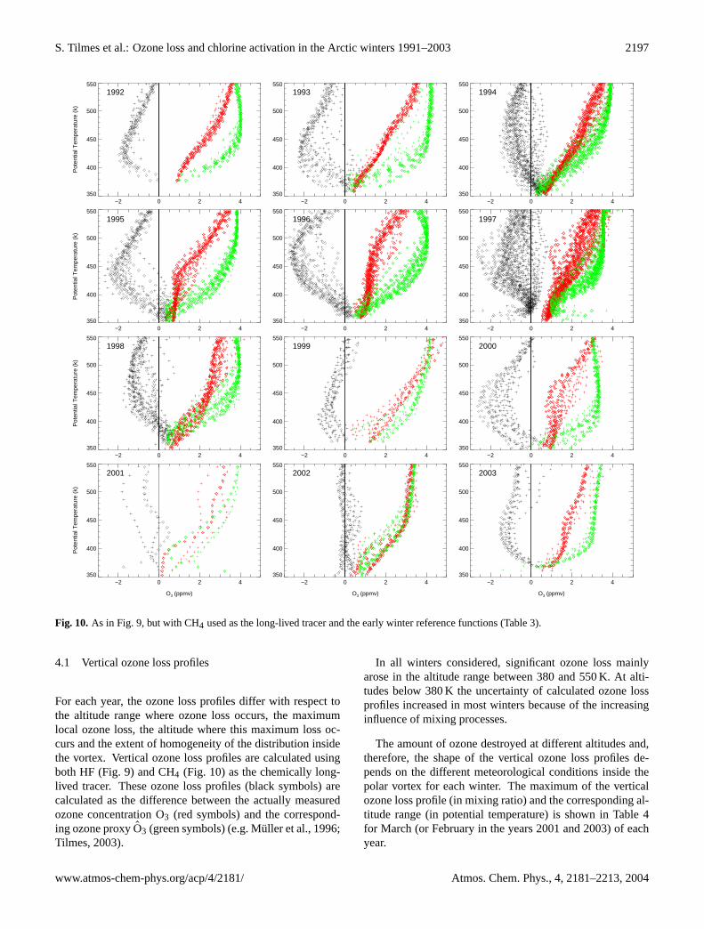
Fig. 10. As in Fig. 9, but with CH4 used as the long-lived tracer and the early winter reference functions (Table 3).
4.1 Vertical ozone loss profiles
For each year, the ozone loss profiles differ with respect tothe altitude range where ozone loss occurs, the maximumlocal ozone loss, the altitude where this maximum loss oc-curs and the extent of homogeneity of the distribution insidethe vortex. Vertical ozone loss profiles are calculated usingboth HF (Fig. 9) and CH4 (Fig. 10) as the chemically long-lived tracer. These ozone loss profiles (black symbols) arecalculated as the difference between the actually measuredozone concentration O3 (red symbols) and the correspond-ing ozone proxyO3 (green symbols) (e.g. Muller et al., 1996;Tilmes, 2003).
In all winters considered, significant ozone loss mainlyarose in the altitude range between 380 and 550 K. At alti-tudes below 380 K the uncertainty of calculated ozone lossprofiles increased in most winters because of the increasinginfluence of mixing processes.
The amount of ozone destroyed at different altitudes and,therefore, the shape of the vertical ozone loss profiles de-pends on the different meteorological conditions inside thepolar vortex for each winter. The maximum of the verticalozone loss profile (in mixing ratio) and the corresponding al-titude range (in potential temperature) is shown in Table 4for March (or February in the years 2001 and 2003) of eachyear.
www.atmos-chem-phys.org/acp/4/2181/ Atmos. Chem. Phys., 4, 2181–2213, 2004

2198 S. Tilmes et al.: Ozone loss and chlorine activation in the Arctic winters 1991–2003
The results derived using two different tracers are withinthe combined uncertainties for each year. To perform a com-parison between the different years, the average of the maxi-mum ozone loss of the two different long-lived tracers is cal-culated (Table 4, column 6). The strongest local ozone lossof all the years considered, about 2.4 ppmv in 1995–1996 and2.5 ppmv 1996–1997, was found in the altitude range fromabout 450–490 K for both winters. In the cold winters of1994–1995 and 1999–2000 the maximum of the local ozoneloss profiles was similarly strong and it occurred for both ofthese winters in the altitude range from about 410–460 K. InMarch 1992 and 1993, local ozone loss is also rather strong,2.0 ppmv in 1992 and 2.2 ppmv in 1993 at very low altitudesin 390–460 K. Winters termed moderately cold, in the sec-tion above, 1991–1992, 1993–1994, 1997–1998 and 2001–2002, show local ozone loss of about 1.5 ppmv, except forthe winter 1991–1992. (The reason for the relatively strongozone loss in 1991–1992 is discussed below). In 2000–2001local ozone loss reached 1.7 ppmv from profiles inside theouter vortex in February only, whereas the local ozone lossprofiles inside the vortex core did not exceed 1.0 ppmv inFebruary 2000–2001 (Fig. 9). In the warm winters, 1998–1999 and 2001–2002, the local ozone loss is 1.0 ppmv and0.4 ppmv, respectively.
As well as the value of the maximum itself, the altituderanges and the width of the peak of the maximum ozone lossdiffers from winter to winter corresponding to the locationof VPSCduring the winter. These factors control the amountof column ozone loss calculated by the vertical integration ofthe ozone loss profile.
In the years 1991–1992, 1992–1993, 1999–2000, 2002–2003, the ozone loss profiles taken inside the vortex corein March (2002–2003 in February) are very homogeneous(Fig. 10). This is the result of an isolated vortex core withhomogeneous ozone loss.
For 1993–1994, 1994–1995, 1995–1996 and 1997–1998,a few profiles of ozone loss indicate a somewhat smaller de-viation from the reference function inside the vortex core butthe majority of ozone loss profiles inside the vortex core arehomogeneously distributed. In 1993–1994 and 1994–1995a warming in February disturbed the isolated vortex. Thevortex shifted off the pole and the cold region was near theedge of the vortex. At this time, rapid ozone destruction oc-curred at the vortex edge (Manney et al., 2003a). The vortexin 1995–1996 and 1997–1998 was already weakening at theend of February and broke down in March. The ozone lossprofiles in 1996–1997 are separated into two distinct partswith moderate loss inside the entire vortex and strong loss inthe vortex core (Tilmes et al., 2003b).
The meteorological developments during the winters de-scribed above may be responsible for inhomogeneous tem-perature distributions inside the vortex. They may be respon-sible for the inhomogeneities in ozone destruction inside theentire vortex, most obvious in winter 1996–1997. In thiswinter inhomogeneities in temperature resulted in inhomo-
geneities in denitrification within the polar vortex (McKennaet al., 2002) that are the likely cause of the inhomogeneitiesin ozone loss (Schulz et al., 2000; Tilmes et al., 2003b).
For most of the years considered here, the calculated ozoneloss profiles for the outer vortex (plus signs in Figs. 9 and 10)show less ozone loss than the profiles in the vortex core. Thetemperatures inside the outer vortex are generally not as lowas inside the vortex core and, therefore, less ozone loss oc-curred inside the outer vortex than inside the vortex core.In some years (March 1994–1995, 1997–1998, 1998–1999and February 2000–2001) a very few profiles show slightlystronger deviations from the reference relation and, there-fore, stronger ozone loss inside the outer vortex than insidethe vortex core. This is possible because exposure to sun-light may be longer inside the outer vortex than inside thevortex core, due to the location of the outer vortex more to-wards lower latitudes. Further discussion of the differencesbetween ozone loss inside the vortex core and the outer vor-tex will be given below in Sect. 4.2.
4.2 Column ozone loss
Column ozone loss for a twelve-year period was derived byintegrating the vertical ozone loss profiles (see AppendixA). This value constitutes a good approximation of the totalamount of ozone loss over the entire column of ozone if thevertical integration is extended over a sufficiently large verti-cal range (≈380–550 K). In this paper, the monthly averagecolumn ozone loss is analysed for altitude ranges between380 and 550 K and between 400–500 K. Further, a compari-son of results of different parts of the polar vortex was per-formed as well as comparison between the results using dif-ferent long-lived tracers.
Tables 5 and 6 summarise the column ozone loss in 380–550 K and in 400–500 K, respectively, averaged over differ-ent months, February, March, April and May (May only inwinter 1996–1997), calculated for each year where measure-ments are available. In February 2000–2001, for two out ofthree profiles measured inside the entire vortex, ozone losswas found only at altitudes above≈450 K (Figs. 9 and 10).These two profiles scatter above the estimated early win-ter reference function at altitudes below 450 K and wouldwrongly increase the calculated ozone loss. Thus, for thiswinter the column ozone loss was calculated for the altituderange between 450 and 500 K only. In Fig. 11 results forthe entire vortex are shown, calculated for the altitude rangeof 380–550 K. The uncertainty of the mean column ozoneloss is described by two parameters. The uncertainty whicharises solely due to the uncertainty of the early winter ref-erence function is shown as a red error bar in Fig. 11. Thestandard deviation of the column ozone loss deduced fromthe individual profiles is shown as a black error bar.
The uncertainty of the early winter reference function isabout 15–25 DU in the altitude range of 380–550 K (Table 5)depending on the scatter of profiles inside the early vortex
Atmos. Chem. Phys., 4, 2181–2213, 2004 www.atmos-chem-phys.org/acp/4/2181/
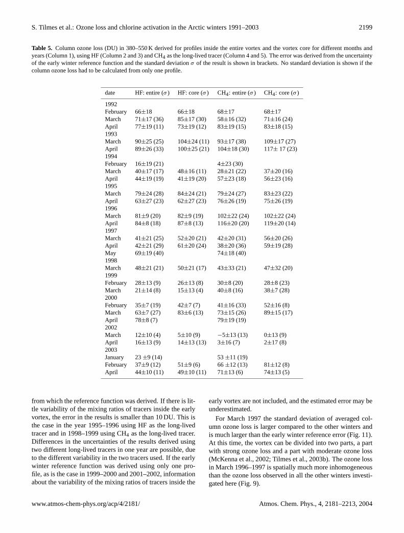
S. Tilmes et al.: Ozone loss and chlorine activation in the Arctic winters 1991–2003 2199
Table 5. Column ozone loss (DU) in 380–550 K derived for profiles inside the entire vortex and the vortex core for different months andyears (Column 1), using HF (Column 2 and 3) and CH4 as the long-lived tracer (Column 4 and 5). The error was derived from the uncertaintyof the early winter reference function and the standard deviationσ of the result is shown in brackets. No standard deviation is shown if thecolumn ozone loss had to be calculated from only one profile.
date HF: entire (σ ) HF: core (σ ) CH4: entire (σ ) CH4: core (σ )
1992February 66±18 66±18 68±17 68±17March 71±17 (36) 85±17 (30) 58±16 (32) 71±16 (24)April 77±19 (11) 73±19 (12) 83±19 (15) 83±18 (15)1993March 90±25 (25) 104±24 (11) 93±17 (38) 109±17 (27)April 89±26 (33) 100±25 (21) 104±18 (30) 117± 17 (23)1994February 16±19 (21) 4±23 (30)March 40±17 (17) 48±16 (11) 28±21 (22) 37±20 (16)April 44±19 (19) 41±19 (20) 57±23 (18) 56±23 (16)1995March 79±24 (28) 84±24 (21) 79±24 (27) 83±23 (22)April 63±27 (23) 62±27 (23) 76±26 (19) 75±26 (19)1996March 81±9 (20) 82±9 (19) 102±22 (24) 102±22 (24)April 84±8 (18) 87±8 (13) 116±20 (20) 119±20 (14)1997March 41±21 (25) 52±20 (21) 42±20 (31) 56±20 (26)April 42±21 (29) 61±20 (24) 38±20 (36) 59±19 (28)May 69±19 (40) 74±18 (40)1998March 48±21 (21) 50±21 (17) 43±33 (21) 47±32 (20)1999February 28±13 (9) 26±13 (8) 30±8 (20) 28±8 (23)March 21±14 (8) 15±13 (4) 40±8 (16) 38±7 (28)2000February 35±7 (19) 42±7 (7) 41±16 (33) 52±16 (8)March 63±7 (27) 83±6 (13) 73±15 (26) 89±15 (17)April 78±8 (7) 79±19 (19)2002March 12±10 (4) 5±10 (9) −5±13 (13) 0±13 (9)April 16±13 (9) 14±13 (13) 3±16 (7) 2±17 (8)2003January 23±9 (14) 53±11 (19)February 37±9 (12) 51±9 (6) 66±12 (13) 81±12 (8)April 44±10 (11) 49±10 (11) 71±13 (6) 74±13 (5)
from which the reference function was derived. If there is lit-tle variability of the mixing ratios of tracers inside the earlyvortex, the error in the results is smaller than 10 DU. This isthe case in the year 1995–1996 using HF as the long-livedtracer and in 1998–1999 using CH4 as the long-lived tracer.Differences in the uncertainties of the results derived usingtwo different long-lived tracers in one year are possible, dueto the different variability in the two tracers used. If the earlywinter reference function was derived using only one pro-file, as is the case in 1999–2000 and 2001–2002, informationabout the variability of the mixing ratios of tracers inside the
early vortex are not included, and the estimated error may beunderestimated.
For March 1997 the standard deviation of averaged col-umn ozone loss is larger compared to the other winters andis much larger than the early winter reference error (Fig. 11).At this time, the vortex can be divided into two parts, a partwith strong ozone loss and a part with moderate ozone loss(McKenna et al., 2002; Tilmes et al., 2003b). The ozone lossin March 1996–1997 is spatially much more inhomogeneousthan the ozone loss observed in all the other winters investi-gated here (Fig. 9).
www.atmos-chem-phys.org/acp/4/2181/ Atmos. Chem. Phys., 4, 2181–2213, 2004
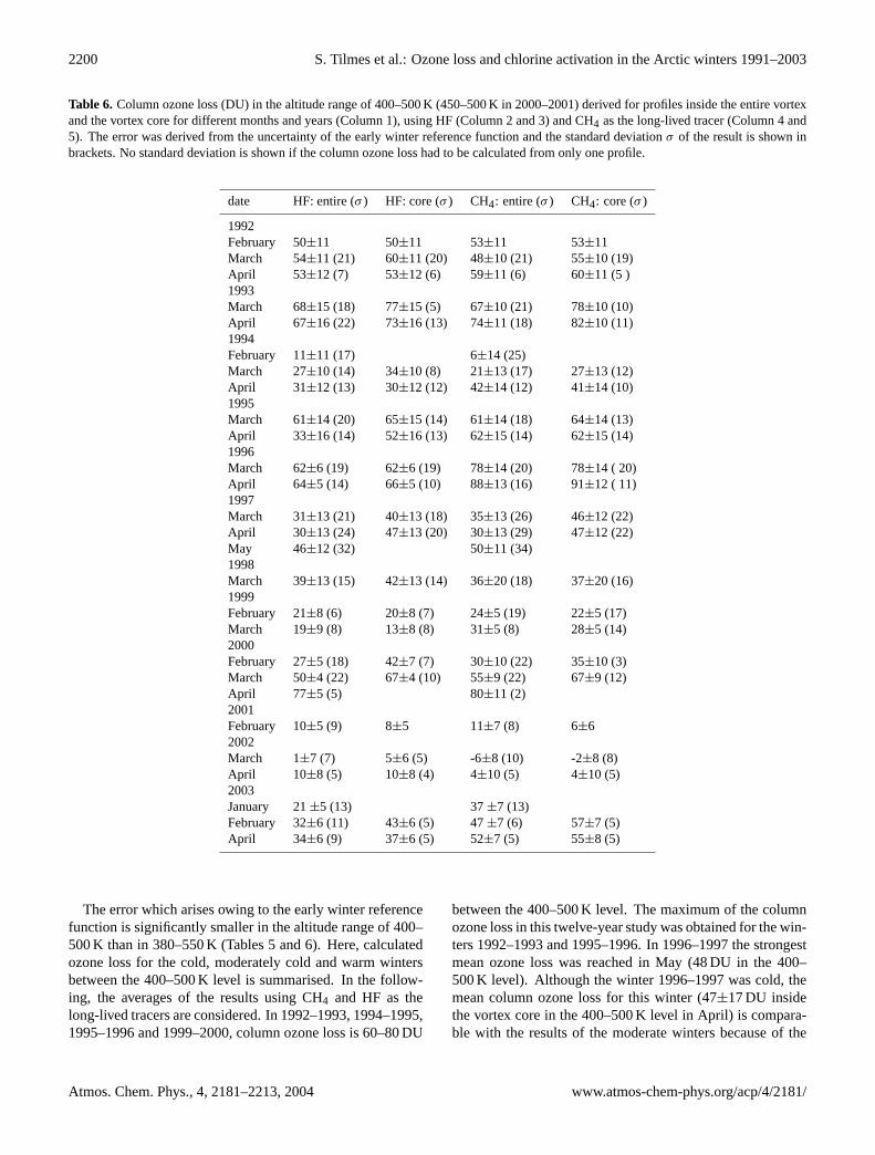
2200 S. Tilmes et al.: Ozone loss and chlorine activation in the Arctic winters 1991–2003
Table 6. Column ozone loss (DU) in the altitude range of 400–500 K (450–500 K in 2000–2001) derived for profiles inside the entire vortexand the vortex core for different months and years (Column 1), using HF (Column 2 and 3) and CH4 as the long-lived tracer (Column 4 and5). The error was derived from the uncertainty of the early winter reference function and the standard deviationσ of the result is shown inbrackets. No standard deviation is shown if the column ozone loss had to be calculated from only one profile.
date HF: entire (σ ) HF: core (σ ) CH4: entire (σ ) CH4: core (σ )
1992February 50±11 50±11 53±11 53±11March 54±11 (21) 60±11 (20) 48±10 (21) 55±10 (19)April 53±12 (7) 53±12 (6) 59±11 (6) 60±11 (5 )1993March 68±15 (18) 77±15 (5) 67±10 (21) 78±10 (10)April 67±16 (22) 73±16 (13) 74±11 (18) 82±10 (11)1994February 11±11 (17) 6±14 (25)March 27±10 (14) 34±10 (8) 21±13 (17) 27±13 (12)April 31±12 (13) 30±12 (12) 42±14 (12) 41±14 (10)1995March 61±14 (20) 65±15 (14) 61±14 (18) 64±14 (13)April 33±16 (14) 52±16 (13) 62±15 (14) 62±15 (14)1996March 62±6 (19) 62±6 (19) 78±14 (20) 78±14 ( 20)April 64±5 (14) 66±5 (10) 88±13 (16) 91±12 ( 11)1997March 31±13 (21) 40±13 (18) 35±13 (26) 46±12 (22)April 30±13 (24) 47±13 (20) 30±13 (29) 47±12 (22)May 46±12 (32) 50±11 (34)1998March 39±13 (15) 42±13 (14) 36±20 (18) 37±20 (16)1999February 21±8 (6) 20±8 (7) 24±5 (19) 22±5 (17)March 19±9 (8) 13±8 (8) 31±5 (8) 28±5 (14)2000February 27±5 (18) 42±7 (7) 30±10 (22) 35±10 (3)March 50±4 (22) 67±4 (10) 55±9 (22) 67±9 (12)April 77±5 (5) 80±11 (2)2001February 10±5 (9) 8±5 11±7 (8) 6±62002March 1±7 (7) 5±6 (5) -6±8 (10) -2±8 (8)April 10±8 (5) 10±8 (4) 4±10 (5) 4±10 (5)2003January 21±5 (13) 37±7 (13)February 32±6 (11) 43±6 (5) 47±7 (6) 57±7 (5)April 34±6 (9) 37±6 (5) 52±7 (5) 55±8 (5)
The error which arises owing to the early winter referencefunction is significantly smaller in the altitude range of 400–500 K than in 380–550 K (Tables 5 and 6). Here, calculatedozone loss for the cold, moderately cold and warm wintersbetween the 400–500 K level is summarised. In the follow-ing, the averages of the results using CH4 and HF as thelong-lived tracers are considered. In 1992–1993, 1994–1995,1995–1996 and 1999–2000, column ozone loss is 60–80 DU
between the 400–500 K level. The maximum of the columnozone loss in this twelve-year study was obtained for the win-ters 1992–1993 and 1995–1996. In 1996–1997 the strongestmean ozone loss was reached in May (48 DU in the 400–500 K level). Although the winter 1996–1997 was cold, themean column ozone loss for this winter (47±17 DU insidethe vortex core in the 400–500 K level in April) is compara-ble with the results of the moderate winters because of the
Atmos. Chem. Phys., 4, 2181–2213, 2004 www.atmos-chem-phys.org/acp/4/2181/

S. Tilmes et al.: Ozone loss and chlorine activation in the Arctic winters 1991–2003 2201
Entire Vortex CH4 380−550 K
92 93 94 95 96 97 98 99 00 01 02 03
Year
0
20
40
60
80
100
120
140
Ozo
ne L
oss
(DU
)
January February March April May
Entire Vortex HF 380−550 K
92 93 94 95 96 97 98 99 00 01 02 03
Year
0
20
40
60
80
100
120
140
Ozo
ne L
oss
(DU
)
January February March April May
Fig. 11. Monthly averaged column ozone loss derived for pro-files inside the entire vortex in 380–550 K, February (green), March(purple), April (orange) and May (yellow) in winters between1991–1992 and 2002–2003. The red error bar indicates the un-certainty of the early winter reference function, the black error barthe standard deviation. Top panel: CH4 was used as the long-livedtracer, bottom panel: HF was used as the long-lived tracer. Ozoneloss was derived from profiles inside the entire vortex.
inhomogeneity of the ozone loss in the vortex. Nonetheless,the maximum local ozone loss of this winter is comparablewith results of the cold winters (Fig. 9).
The moderately cold winters 1991–1992, 1993–1994,1997–1998 and 2002–2003 reach a mean column ozone lossbetween 31 DU (in winter 1994–1995) and 57 DU (in win-ter 1991–1992) inside the vortex core in March. (Results ofwinter 2002–2003 using CH4 as the long-lived tracer are ex-cluded due to uncertain data, as discussed below). In 2000–2001, the mean column ozone loss was deduced for Februaryin 450–500 K, as described above. Only 10 DU were calcu-lated for the entire vortex. Nevertheless, the maximum col-umn ozone loss reached 20±4 DU and 21±6 DU using HFand CH4 as the long-lived tracers for one profile inside theouter vortex in 450–500 K. In the warm winter 1998–1999ozone loss still reaches 25±10 DU derived for an altituderange of 400–500 K from profiles inside the entire vortex and21±10 DU for profiles inside the vortex core. Inside the en-tire vortex in March 2002 no ozone loss is diagnosed withthe TRAC technique within the uncertainty of the early win-ter reference function.
Entire Vortex CH4 − HF 380−550 K
92 93 94 95 96 97 98 99 00 01 02 03
Year
−40
−20
0
20
40
Ozo
ne L
oss
(DU
)
January February March April May
Thu Mar 11 10:04:58 2004imone/IDL/HALOE_PRO/haloe_intern_set_plot.pro LOSS_ALL/loss_40ch4_hf_diff380_550.psFig. 12. Difference between monthly averaged column ozone lossderived for profiles inside the entire vortex in 380–500 K using HFand CH4 as the long-lived tracer (see Fig. 11 top and bottom panel).Ozone loss was derived from profiles inside the entire vortex.
The exact mean calculated column ozone loss differs de-pending on whether HF or CH4 is used as the long-livedtracer. Further, ozone loss differs depending whether the vor-tex core or the entire vortex is considered. In Fig. 12, thedifference between the ozone loss derived with the two long-lived tracers are shown.
The differences between the results using HF and CH4 aslong-lived tracers are≈10–20 DU for most of the observedyears and are similar for the entire vortex and the vortex core(not shown). The smallest differences are calculated for win-ters 1996–1997 and 1997–1998 (below 5 DU). The differ-ence in the early winter reference functions using the twodifferent long-lived tracers are mostly responsible for the dif-ferent results. In most years observed the results obtainedusing CH4 as the long-lived tracer agree with those using HFwithin the uncertainty introduced by the uncertainty of thereference function.
In some years, ozone loss calculated by employing CH4 asthe long-lived tracer has a tendency towards larger ozone losstoward the end of the winter compared to HF (Fig. 11). Espe-cially in March 1996, the results differ by more than 30 DUfor the entire vortex. In winter 2002–2003 results derived us-ing CH4 as the long-lived tracer are significantly larger (25–30 DU) than using HF during the entire winter period. TheCH4 mixing ratios inside the Arctic vortex at altitudes belowabout 450 K may be problematic in these years, due to sig-nal saturation problems. Such problems are also discussedfor the winter 1999–2000 by Muller et al. (2002) and may beresponsible for the differences between the results of the twodifferent long-lived tracers used in 2002–2003 (Tilmes et al.,2003a). Therefore, results derived employing CH4 as thelong-lived tracer are not discussed in Tilmes et al. (2003a).Also, the significant discrepancies between the results of thetwo different long-lived tracers in March 1996 may be ex-plained by this problem.
www.atmos-chem-phys.org/acp/4/2181/ Atmos. Chem. Phys., 4, 2181–2213, 2004

2202 S. Tilmes et al.: Ozone loss and chlorine activation in the Arctic winters 1991–2003
Table 7. Calculated chemical loss in column ozone loss in the Arctic in winters 1993–1994 to 2001–2002. Comparison between HALOEresults and results from other methods.
date SAOZ/ SAOZ/ Match [DU] HALOE [DU] HALOE [DU]REPROBUS [%] REPROBUS [DU] entire vortex vortex core
in 380–600 K in 370–700 K in 380–550 K in 380–550 K
Jan–Mar 1994 7 31 34±23 43±22mid-Jan–Mar 1995 21 95 108±18 77±27 82±27mid-Jan–Mar 1996 20 83 92±25 93±25Jan–Mar 1997 22 110 46±22 61±22Jan–Mar 1998 12 57 46±35 49±33Dec–Mar 1999 5 25 31±24 27±24Dec–Mar 2000 23 105 68±12 86±15Jan–Apr 2002 7 32 10±21 8±20
Entire Vortex − Vortex Core 380−550 K
92 93 94 95 96 97 98 99 00 01 02 03
Year
−20
−10
0
10
20
Ozo
ne L
oss
(DU
)
January February March April May
Thu Mar 11 09:59:45 2004imone/IDL/HALOE_PRO/haloe_intern_set_plot.pro LOSS_ALL/loss_diffch4,hf380_550.psFig. 13. Difference of monthly averaged column ozone loss be-tween the entire vortex and the vortex core for all winters between1991–1992 and 2002–2003, using both CH4 and HF as the long-lived tracers. Results were derived in an altitude range of 380–550 K.
Inside the outer vortex, the mean column ozone loss is inmost cases less than inside the vortex core (Fig. 13) due totemperature differences, as described above. This effect isvery strong for winters 1991–1992, 1992–1993, 1996–1997,1999–2000 and 2002–2003. As already found consideringthe vertical ozone loss profiles, in some years the ozone lossis insignificantly greater inside the outer vortex than insidethe vortex core (in April 1992, 1994 and 1995, February andMarch 1999 and February 2001). Further, in some years thestandard deviation for profiles in the outer vortex is signifi-cantly larger than inside the vortex core (1992–1993, 1994–1995, 1995–1996 and 1999–2000) (see Tables 5 and 6). Thatis because the ozone loss inside the outer vortex was muchmore inhomogeneous than in the vortex core in these winters.
5 Comparison with ozone loss estimates using differentmethods
The results deduced here using the TRAC method are com-pared with published results obtained by different methodsfor the determination of chemical ozone loss. Chemicalozone loss in the Arctic vortex in the past decade has been es-timated by a variety of methods for different winters (Harriset al., 2002; Newman et al., 2002). However, a comparisonbetween the different ozone loss estimates is only meaningfulif the figures compared are determined for exactly the sameconditions (Harris et al., 2002).
5.1 Comparison of column ozone losses
Column ozone loss from the SAOZ/REPROBUS approach(Goutail et al., 1999; Deniel et al., 1998; Lefevre et al., 1998)was estimated for a period from December to March/Aprilfor winters 1993–1994 to 2002–2003 (Goutail et al., 2000,2003) at altitudes between 380 and 600 K. The TRAC tech-nique estimates ozone loss between the time when the ref-erence function was derived (see Fig. 1) and the time whenHALOE measurements are available in March/April in alti-tudes between 380 and 550 K. Considering slightly differentaltitudes for SAOZ and TRAC has little impact on the to-tal column ozone loss. The early winter reference functionin winter 1993–1994 was derived from observations at theend of November and at the beginning of January. Duringthese two month no ozone loss was found inside range ofuncertainty of the early winter reference function (≈20 DU).To compare the results, ozone loss from SAOZ is also con-sidered for the period between January and March 1994. Inthis winter, SAOZ estimated≈10% ozone loss in December(Goutail et al., 1999) and≈7% between January and March.If an average of 441 DU is taken from the inert tracer simula-tions in March 1994 (pers. comm., F. Goutail, 2004), 31 DUozone loss is estimated for the period between January andMarch 1994 from SAOZ (Table 7), which agrees well with
Atmos. Chem. Phys., 4, 2181–2213, 2004 www.atmos-chem-phys.org/acp/4/2181/

S. Tilmes et al.: Ozone loss and chlorine activation in the Arctic winters 1991–2003 2203
the accumulated ozone derived from HALOE measurementsusing the TRAC technique.
In winter 1994–1995, the early winter reference func-tion was derived in mid-January. Therefore, SAOZ ozoneloss is estimated for the period between mid-January andMarch (Goutail et al., 2003) (≈21% or 95 DU, where 452 DUis the approximated passive ozone). This result is some-what greater than that derived from TRAC using HALOEobservations, although inside the range of uncertainty (Ta-ble 7).
The early winter reference function in 1995–1996 wasderived from both November and January profiles. As for1993–1994 no ozone loss was found during these two monthswithin the range of uncertainty. SAOZ accumulated ozoneloss in winter 1995–1996 between mid-January and Marchis ≈20% (83 DU). This value is in good agreement withHALOE results. For 1996–1997 the result from SAOZagrees with the largest ozone loss calculated by TRAC in-side the vortex core (90–110 DU), but the averages do notagree.
In winters 1997–1998 and 1998–1999, the results ofSAOZ and TRAC using HALOE data agree within the re-ported uncertainty. The estimated ozone loss from SAOZ inwinters 1999–2000, 2001–2002 is≈20 DU larger than de-rived here from TRAC.
The very large ozone loss rates in the early winter 1993–1994, 1994–1995, 1995–1996 and 1997–1998 derived bySAOZ can neither be confirmed nor falsified using HALOEmeasurements due to the lack of observations. However, inthe TRAC analysis there is no sign of such strong ozonelosses as deduced by SAOZ in January 1993–1994 and 1995–1996, when HALOE measurements are available only withinthe vortex boundary region.
Chemical ozone loss was derived by the Match techniquefor the winter 1994–95 (Rex et al., 1998; Schulz et al., 2000)for the period between January 1 and March 1995, in 370–700 K. It is more than 40 DU larger (127±14 DU) than thatwith HALOE (in 380–550 K). Like SAOZ, the Match tech-nique estimated strong ozone loss during the first two weeksin January. Because the temporal evolution of ozone de-struction estimated by SAOZ and Match coincides quiet well(Rex et al., 1998) in this year, we assume that about onethird of the ozone loss derived by Match occurred during thefirst half of January. This results in accumulated ozone lossof 108±18 DU estimated from Match results, which agreeswith HALOE results within the range of uncertainty (Ta-ble 7).
The column ozone loss from UARS microwave limbsounder (MLS) measurements for March (end of February1997) of the winters 1991–1992 to 1996–1997 was calcu-lated for above 100 hPa (Manney et al., 2003a). These resultsare compared with HALOE results derived for the altituderange of 40 to 100 hPa (Table 8) to allow a direct compar-ison with the MLS results. The results of the two methodsagree in so far as the strongest ozone loss was found for the
winters 1995–1996 and 1992–1993. Nevertheless, signifi-cant differences occur because the time intervals consideredusing the two techniques are not exactly the same (Manneyet al., 2003a). The strongest discrepancies arise for the win-ters 1991–92 and 1994–95 (see Table 8, fifth column).
In 1991–1992 the ozone loss from MLS was derived ina period between 12 January and 22 March 1992 (Manneyet al., 2003a). At the beginning of January 1992, a largeVPSCand significant solar insolation already existed. There-fore ozone loss occurred before the start of the calculationusing MLS measurements, which at least partly explains thelarger ozone loss deduced from TRAC compared to MLS.Ozone loss in winter 1994–1995 was estimated in the periodbetween 21 December 1994 and 10 March 1995 using MLSobservations. The second part of March PSCs are possible ataltitudes below 500 K (see Fig. 1) and the vortex was stronglyilluminate in spring. Ozone loss calculated for March 1995using the TRAC method includes the loss in the second partof March, whereas MLS calculations stopped at 10 March1995. Therefore, significantly smaller ozone losses were es-timated using MLS.
For the winter 1992–1993, MLS calculations were startedone month later than here using HALOE measurements. In-deed, results derived using MLS data are slightly lower. Inwinter 1993–1994 and 1995–1996, the ozone losses deter-mined from MLS data and HALOE measurements are wellinside the range of uncertainty. A quite similar period wasconsidered for both methods to derive chemical ozone loss.In 1996–1997, MLS calculations of ozone loss stopped at theend of February 1997. However, in March significant ozoneloss can be expected (Tilmes et al., 2003b; Terao et al., 2002).Although, ozone loss deduced with the two approaches fitsvery well in this winter considering the entire vortex, MLSozone loss is significantly smaller considering the vortexcore.
In summary, all the differences occurring between ozoneloss derived using MLS data, on the one hand, and the TRACmethod using HALOE data, on the other hand, can be ex-plained by the fact that different time intervals are consideredfor the derivation of chemical ozone loss.
In winter 1999–2000, the column ozone loss inside theArctic was derived from various measurements and by dif-ferent techniques because an extensive measurement cam-paign was conducted: SOLVE-THESEO 2000 (Newmanet al., 2002). The ozone loss calculated between early Jan-uary and mid-March by the Match technique is 71±12 DU(Rex et al., 2002). Results from the OMS balloon mea-surements (Salawitch et al., 2002) were calculated up to 5March 2000 as 61±14 DU. An extrapolation of the resultfor 5 March to mid-March (based on Match-derived ozoneloss rates (Muller et al., 2002) yielded 84±13 DU. Ozoneloss from POAM/REPROBUS was determined as 80 DU in380–700 K, as reported by Harris et al. (2002). These resultsagree well with the column ozone loss found in the presentwork (86±15 DU in 380–550 K inside the vortex core).
www.atmos-chem-phys.org/acp/4/2181/ Atmos. Chem. Phys., 4, 2181–2213, 2004
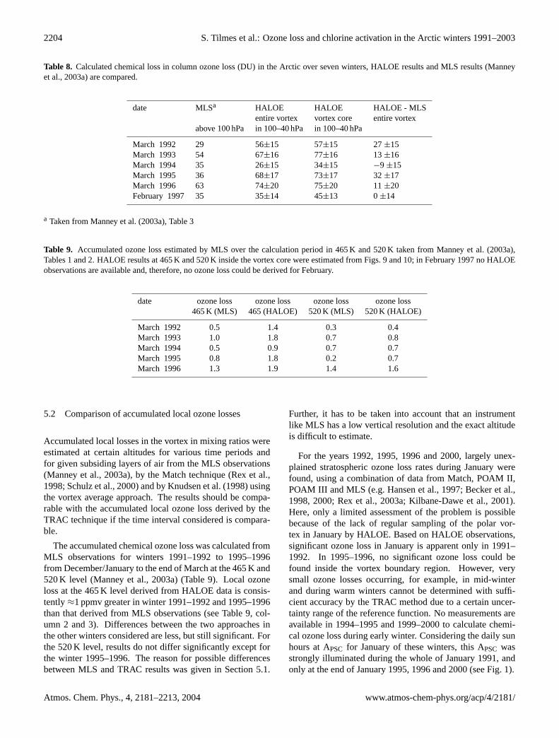
2204 S. Tilmes et al.: Ozone loss and chlorine activation in the Arctic winters 1991–2003
Table 8. Calculated chemical loss in column ozone loss (DU) in the Arctic over seven winters, HALOE results and MLS results (Manneyet al., 2003a) are compared.
date MLSa HALOE HALOE HALOE - MLSentire vortex vortex core entire vortex
above 100 hPa in 100–40 hPa in 100–40 hPa
March 1992 29 56±15 57±15 27±15March 1993 54 67±16 77±16 13±16March 1994 35 26±15 34±15 −9 ±15March 1995 36 68±17 73±17 32±17March 1996 63 74±20 75±20 11±20February 1997 35 35±14 45±13 0±14
a Taken from Manney et al. (2003a), Table 3
Table 9. Accumulated ozone loss estimated by MLS over the calculation period in 465 K and 520 K taken from Manney et al. (2003a),Tables 1 and 2. HALOE results at 465 K and 520 K inside the vortex core were estimated from Figs. 9 and 10; in February 1997 no HALOEobservations are available and, therefore, no ozone loss could be derived for February.
date ozone loss ozone loss ozone loss ozone loss465 K (MLS) 465 (HALOE) 520 K (MLS) 520 K (HALOE)
March 1992 0.5 1.4 0.3 0.4March 1993 1.0 1.8 0.7 0.8March 1994 0.5 0.9 0.7 0.7March 1995 0.8 1.8 0.2 0.7March 1996 1.3 1.9 1.4 1.6
5.2 Comparison of accumulated local ozone losses
Accumulated local losses in the vortex in mixing ratios wereestimated at certain altitudes for various time periods andfor given subsiding layers of air from the MLS observations(Manney et al., 2003a), by the Match technique (Rex et al.,1998; Schulz et al., 2000) and by Knudsen et al. (1998) usingthe vortex average approach. The results should be compa-rable with the accumulated local ozone loss derived by theTRAC technique if the time interval considered is compara-ble.
The accumulated chemical ozone loss was calculated fromMLS observations for winters 1991–1992 to 1995–1996from December/January to the end of March at the 465 K and520 K level (Manney et al., 2003a) (Table 9). Local ozoneloss at the 465 K level derived from HALOE data is consis-tently≈1 ppmv greater in winter 1991–1992 and 1995–1996than that derived from MLS observations (see Table 9, col-umn 2 and 3). Differences between the two approaches inthe other winters considered are less, but still significant. Forthe 520 K level, results do not differ significantly except forthe winter 1995–1996. The reason for possible differencesbetween MLS and TRAC results was given in Section 5.1.
Further, it has to be taken into account that an instrumentlike MLS has a low vertical resolution and the exact altitudeis difficult to estimate.
For the years 1992, 1995, 1996 and 2000, largely unex-plained stratospheric ozone loss rates during January werefound, using a combination of data from Match, POAM II,POAM III and MLS (e.g. Hansen et al., 1997; Becker et al.,1998, 2000; Rex et al., 2003a; Kilbane-Dawe et al., 2001).Here, only a limited assessment of the problem is possiblebecause of the lack of regular sampling of the polar vor-tex in January by HALOE. Based on HALOE observations,significant ozone loss in January is apparent only in 1991–1992. In 1995–1996, no significant ozone loss could befound inside the vortex boundary region. However, verysmall ozone losses occurring, for example, in mid-winterand during warm winters cannot be determined with suffi-cient accuracy by the TRAC method due to a certain uncer-tainty range of the reference function. No measurements areavailable in 1994–1995 and 1999–2000 to calculate chemi-cal ozone loss during early winter. Considering the daily sunhours at APSC for January of these winters, this APSC wasstrongly illuminated during the whole of January 1991, andonly at the end of January 1995, 1996 and 2000 (see Fig. 1).
Atmos. Chem. Phys., 4, 2181–2213, 2004 www.atmos-chem-phys.org/acp/4/2181/

S. Tilmes et al.: Ozone loss and chlorine activation in the Arctic winters 1991–2003 2205
In winter 1996–1997, accumulated ozone loss was esti-mated in the period between the end of January and the end ofMarch by the Match technique (1.1 ppmv) and by using thevortex average approach (0.9±0.2 ppmv) at the 455 K poten-tial temperature level (Harris et al., 2002). Such values are inagreement with the moderate ozone loss within the range ofuncertainty deduced from ILAS 0.5–1.0 ppmv (±0.2 ppmv)and HALOE 0.9–1.4 ppmv (±0.2 ppmv) at the 475 K level(Tilmes et al., 2003b). Further calculations of ozone losswere performed by the Match technique based on ILAS ob-servations for the winter 1996–1997 (Terao et al., 2002).There, the integrated ozone loss during February and Marchreached 2.0±0.1 ppmv at 475–529 K levels. This result is ingood agreement with the maximum of the ozone loss profileof 2.0±0.3 ppmv derived from ILAS by the TRAC techniquein a similar altitude range (Tilmes et al., 2003b).
However, in winter 1996–1997 vortex average losses ob-tained by different methods are very difficult to compare be-cause ozone loss inside the vortex was spatially very inhomo-geneous (McKenna et al., 2002; Schulz et al., 2000; Tilmeset al., 2003b). Thus, the averages derived will greatly dependon what fraction of the data entering the average originatesfrom the vortex region showing the stronger ozone loss.
In 1999–2000 HALOE local ozone loss in 430–450 K(2.3±0.2 ppmv) is in good agreement with the accumulatedozone loss in the vortex in mid-March derived by the Matchtechnique (2.0±0.3 ppmv) (Rex et al., 2002). The ozoneand the tracer measurements between early January and mid-March 2000 from the ER-2 were used to deduce chemicalozone loss (1.8±0.3 ppmv) (Richard et al., 2001). Ozone lossdeduced from POAM III satellite measurements only reached1.5±0.3 ppmv for mid-March (Hoppel et al., 2002).
The accumulated ozone loss derived using the vortexaverage approach (Rex et al., 2004) agrees most closely withthe results derived using the TRAC technique, as will bedescribed below in detail in Sect. 6.
6 Impact of meteorological conditions on ozone loss
Arctic ozone loss is related to the particular meteorologicaland dynamic conditions of the polar vortex in each year. Thetwelve-year time series of ozone loss obtained in a consistentmanner in this paper allows this question to be addressed indetail. In this section, the relationship between accumulatedozone loss and the volume of possible PSC existence (VPSC)– also referred to as potential volume of PSCs (Rex et al.,2004) – will be derived and compared with the results of thefirst study (Rex et al., 2004) of this relationship. Further,the impact of different factors – such as the amount of solarillumination on PSC area – on ozone loss are discussed indetail.
1992 1994 1996 1998 2000 2002 2004
years
0
20
40
60
80
VP
SC
Mid−Dec to MarchNov to AprilEarly Ref. to MarchJanuary
1992 1994 1996 1998 2000 2002 2004
years
0
2
4
6
8
Sun
hou
rs p
er d
ay a
t AP
SC
Mid−Dec to MarchNov to AprilEarly Ref. to MarchJanuary
Fig. 14. Daily mean VPSC (top panel) and sun hours at possiblearea of PSC existence, VPSC(bottom panel) averaged between 400–550 K in the Arctic polar vortex using UKMO data for the years1991–1992 to 2002–2003 in different colours. Different symbolsindicate different time intervals for calculating the averaged dailymean: stars: entire January; filled squares: from early winter ref-erence function to end of March; filled diamonds: entire winter pe-riod; filled circles: mid-December to end of March; open circles:mid-December to end of March (Rex et al., 2004).
Before referring to the relationship between accumulatedozone loss and VPSC, each of these values will be discussedseparately. Accumulated ozone loss in DU and in mixing ra-tios was estimated in the pervious sections for different timeintervals depending on available measurements inside the po-lar vortex core. In detail, the results were derived for the pe-riod between the date of the early winter reference function– varying each year (see Fig. 1) – and February, March andApril. In the following, accumulated ozone loss calculatedfor March (in 2000–2001 and 2002–2003 for February) isconsidered in altitude ranges between 380 and 550 K and be-tween 400 and 500 K. Ozone loss of the winter 2000–2001was derived for an altitude range of 450–500 K only (as de-scribed in Sect. 4.2). Further, the results of the very warmwinter 2001–2002 have a large uncertainty that can only be
www.atmos-chem-phys.org/acp/4/2181/ Atmos. Chem. Phys., 4, 2181–2213, 2004

2206 S. Tilmes et al.: Ozone loss and chlorine activation in the Arctic winters 1991–2003
0 10 20 30 40
VPSC (106 km3)
0
50
100
Ozo
ne lo
ss (
DU
)
1991/1992 1992/1993 1993/1994 1994/1995 1995/1996 1996/1997 1997/1998 1998/1999 1999/2000 2000/2001 2001/2002 2002/2003
Fig. 15. Relation between the accumulated ozone loss in DUand VPSC in the Arctic polar vortex for the years 1991–1992 to2002–2003 in different colours. Monthly averaged ozone loss in-side the vortex core in March (February 2002–2003) between 380–550 K (winter 2000–2001 is not included) using the TRAC method;coloured solid squares (HF is used as the long-lived tracer) and soliddiamonds (CH4 is used as the long-lived tracer). Ozone loss de-rived by the vortex average approach (Rex et al., 2004) is shown incoloured open circles for the same altitude range. VPSC, taken fromRex et al. (2004), was averaged between mid-December to Marchof each year and between 400–550 K derived from ECMWF data.Black line indicates a linear relation between VPSCand ozone lossfrom the TRAC method. Green line indicates the linear relationbetween VPSC and ozone loss from the vortex average approachreported by Rex et al. (2004).
poorly quantified because the vortex was not isolated andthese results are not considered. Additionally, the results ofwinters 1997–1998 and 2000–2001 have to be regarded withcaution because the early winter reference functions had tobe derived from the climatology values.
The PSC occurrence varies for different winters dependingon the evolution of temperature and dynamics of the polarvortex (Fig. 8). To compare PSC occurrences, an averagevalue over a certain time interval and a certain altitude rangehas to be calculated. These averaged VPSC values stronglydepend on the time interval considered (see Fig. 14).
In Fig. 14, top panel, the daily average VPSC are shownfor different time intervals. The calculation of VPSCover theentire winter period from November to the end of April indi-cates the temperature conditions for the entire winter. Basedon VPSC, a classification of the Arctic winters into cold,moderately cold, and warm winters is possible (see end ofSect. 3).
Each winter differs decisively in the temperature evolu-tion. Some winters are very cold in January (1999–2000),(Fig. 14, top panel, filled squares), whereas others are muchcolder in December (2002–2003) or in February and March(1996–1997). This information cannot be captured in an av-erage of the entire winter, nor is it covered in an averagebetween mid-December and the end of March, as used byRex et al. (2004). Further, the difference between VPSC av-eraged for different time intervals in any given year stronglydepends on the year considered.
As the daily average VPSC is derived for different time in-tervals, sun hours per day are averaged on a possible areaof PSC (APSC) based on UKMO meteorological analysis(Fig. 14, bottom panel). The amount of solar insolation atonly the cold parts of the polar vortex depends on the timeinterval considered as well. During January, sun hours perday vary between 0.5 sun hours per day (1992–1993) up to 5sun hours per day in winter 2001–2002. Sun hours per dayaveraged for the time interval between the time of the earlywinter reference function and the end of March vary between2 sun hours per day in winter 1999–2000 up to above 6 sunhours per day in winter 1994–1995. The influence of thevariations of solar insolation between different years will bediscussed further below.
The relationship between accumulated ozone loss andthe daily average VPSC has been reported by Rex et al.(2004). They averaged VPSC in the time interval betweenmid-December and the end of March based on meteorologi-cal analysis from ECMWF (Fig. 14, top panel, coloured opencircles). In the present study, VPSCwas determined from theUKMO analysis in the same altitude range (400–550 K) andin the same time interval as by Rex et al. (2004) (Fig. 14, toppanel, filled circles). Some differences arise between VPSCderived from Rex et al. (2004) and this study. This is possiblyowing to the different meteorological analysis used (Manneyet al., 2003a).
Accumulated ozone loss in mixing ratios calculated usingthe vortex average approach is averaged between day 15 andday 85 of a particular year in a vertical region between 14 and24 km (Rex et al., 2004). In winter 1994 and 1999 the timeinterval of days 25 to 85 was chosen (late establishment ofthe vortex). In winter 1992, 1998 and 2003 the time intervalof days 15 to 75 was chosen (early break up). The lower limitof the range is 380 K and the upper limit is≈550 K.
The accumulated ozone loss derived using the vortex aver-age approach (Rex et al., 2004) and the results derived in thisstudy are comparable using ozone loss derived in 380–550 K.The relationship between these results and the daily averageVPSCderived by Rex et al. (2004) is shown in Fig. 15.
The green line indicates the linear relationship reported byRex et al. (2004). HALOE ozone loss values show a quitesimilar relationship. The slope (black line) is somewhat less(1.8 DU per 106 km3) compared to the green line (2.1 DU per106 km3) owing to the much larger ozone loss values of thewinters 1991–1992 and 1992–1993 derived using the TRACmethod. Accumulated ozone loss of the two approaches iswell inside their range of uncertainty (reported uncertaintyof the vortex average approach is 10–15 DU), except for thewinters 1991–1992 and 1992–1993. These two winters showsignificant deviations from the linear relations that are pos-sibly due to the impact of an enhanced stratospheric aerosolcontent in these years, as will be discussed below. This in-fluence was also found by Rex et al. (2004), although it ismuch smaller (with a maximum of≈10 DU for total ozoneloss calculated between 14 and 24 km) than that derived here.
Atmos. Chem. Phys., 4, 2181–2213, 2004 www.atmos-chem-phys.org/acp/4/2181/

S. Tilmes et al.: Ozone loss and chlorine activation in the Arctic winters 1991–2003 2207
One reason for the discrepancy between the two approachesmay be that Rex et al. (2004) started their ozone loss calcu-lation at day 15 (25) of the year in question. This is aboutone month later than the start of ozone loss calculation usingthe TRAC method (Fig. 1). Especially in 1991–1992, a largePSC volume and significant solar insolation already existedbefore day 15 of the year 1992 (as already discussed com-paring HALOE and MLS results). For the same reason, theaverage approach may calculate smaller values of ozone lossin winters 1992–1993, 1993–1994, 1997–1998, and 2002–2003 (winter 2000–2001 and 2001–2002 were not consid-ered) (see Fig. 15). On the other hand, in winters 1994–1995and 1995–1996 the start of ozone loss calculation was laterusing the TRAC technique compared to the vortex averageapproach, and PSCs and significant daily solar radiation werepresent before this time. Therefore, ozone loss derived usingTRAC should be smaller compared to the result of the vor-tex average approach. The described discrepancies (exceptfor the winter 1994–1995) are obvious in Fig. 15, althoughin most of the years considered the error bar is much largerthan the discrepancies.
Considering a time interval for estimating VPSCfrom mid-December to the end of March, further important factors con-trolling ozone loss are masked by averaging VPSCover nearlythe entire winter. In the next part of this section, differenttime intervals to average VPSCwill be used to perform a com-parison between chemical ozone loss calculated using theTRAC method and VPSC. For this purpose, both parameters(ozone loss and VPSC) are estimated in the same time intervalbetween the time of the early winter reference function andthe end of March (February in 2000–2001 and 2002–2003)using the TRAC technique. Further, accumulated ozone losswas derived for an altitude range of 400–500 K, because herethe error is less compared to larger altitude ranges using theTRAC method (see Sect. 2.2). As described above, resultsof the winters 1997–1998 and 2000–2001, and especially ofthe very warm winter 2001–2002, have to be regarded withcaution.
Under these conditions, ozone loss and VPSC show a lin-ear relationship as well. This relationship is derived fromall the values shown in Fig. 16. The slope is 1.1 DU per106 km3 using accumulated column ozone loss and 0.7 ppmvusing ozone loss in mixing ratios averaged between 400 and500 K (Fig. 16, black lines). The slope is less than in Fig. 15,because ozone loss was derived in a smaller altitude range.Further, a stronger deviation from a linear relationship oc-curs. Especially the winter 1994–1995 deviates significantlyfrom the derived linear relationship.
Besides VPSC, chemical ozone destruction is expected tobe influenced by the duration of the exposure to sunlight ofthe cold vortex regions, because solar radiation is involvedin ozone-destroying cycles. Additionally, this effect was al-ready found for the January ozone loss in Sect. 3.1
To separate different factors controlling ozone loss, andthus to eliminate the effect of VPSC on ozone depletion, we
0 10 20 30 40
VPSC (106 km3)
−20
0
20
40
60
80
100
Ozo
ne lo
ss (
DU
)
1991/1992 1992/1993 1993/1994 1994/1995 1995/1996 1996/1997 1997/1998 1998/1999 1999/2000 2000/2001 2001/2002 2002/2003
0 10 20 30 40
VPSC (106 km2)
0.0
0.5
1.0
1.5
2.0
Ozo
ne lo
ss (
ppm
v)
1991/1992 1992/1993 1993/1994 1994/1995 1995/1996 1996/1997 1997/1998 1998/1999 1999/2000 2000/2001 2001/2002 2002/2003
Fig. 16. Top panel: relation between the column ozone loss (DU)and VPSC in the Arctic polar vortex for the years 1991–1992 to2002–2003 in different colours. Monthly averaged ozone loss insidethe vortex core in March (February in 2000–2001 and 2002–2003)between 400–500 K (between 450–500 K inside the entire vortex inwinter 2000–2001) using the TRAC method; coloured solid squares(HF is used as the long-lived tracer) and solid diamonds (CH4 isused as the long-lived tracer). VPSCwas averaged between the timeof the early winter reference function of each year and the end ofMarch between 400–550 K derived from UKMO data. Black lineindicates a linear relation between VPSC and ozone loss. Bottompanel: as top panel, but for the accumulated ozone loss in mixingratio in the altitude range 400–500 K derived only from HALOEobservations is shown.
consider the deviation of ozone loss values from the linearrelation between ozone loss and VPSC(black lines in Fig. 16,that is a fit through the entire set of values). We will hereafterrefer to this quantity as the “ozone loss anomaly”. In Fig. 17,the ozone loss anomaly is plotted against sun hours per day.The latter quantity was calculated only for the cold partsof the vortex (that is only for temperatures below the PSCthreshold). Daily sun hours at possible APSC were averagedin a time interval between the time of early winter referencefunction and the end of March between 400–550 K. Exclud-ing the winters 1991–1992 and 1992–1993 (strong influenceof volcanic eruption) and 2000–2001 and 2001–2002 (uncer-tain results) a linear relation between the ozone loss anomalyand sun hours per day is obvious. The slope is 8.9 DU persun hour withσ=9.1 DU considering the accumulated ozoneloss. Considering ozone loss in mixing ratios, the slope is
www.atmos-chem-phys.org/acp/4/2181/ Atmos. Chem. Phys., 4, 2181–2213, 2004

2208 S. Tilmes et al.: Ozone loss and chlorine activation in the Arctic winters 1991–2003
2 3 4 5 6
Sun hours per day at Apsc
−40
−20
0
20
40
Ozo
ne lo
ss a
nom
aly(
DU
)
(
(
)
)
1991/1992 1992/1993 1993/1994 1994/1995 1995/1996 1996/1997 1997/1998 1998/1999 1999/2000 2000/2001 2001/2002 2002/2003
2 3 4 5 6
Sun hours per day at Apsc
−1.0
−0.5
0.0
0.5
1.0
Ozo
ne lo
ss a
nom
aly
(ppm
v)
((
))
1991/1992 1992/1993 1993/194 1994/1995 1995/1996 1996/1997 1997/1998 1998/1999 1999/2000 2000/2001 2001/2002 2002/2003
Fig. 17. Top panel: deviation of column ozone loss (DU) fromthe linear relation (black line in Fig. 16, top panel) in relation tosun hours per day at (APSC) (see text). Bottom panel: deviationof accumulated ozone loss in mixing ratio from the linear relation(black line in Fig. 16, bottom panel) in relation to sun hours per dayat (APSC) (see text).
0.23 ppmv withσ=0.22 ppmv (Fig. 17, black lines). The ef-fect of different durations of illumination on the cold parts ofthe polar vortex is therefore significant. An increase in sunhours per day of 4 h may result in an increase of≈36 DUcolumn ozone loss inside the vortex core, or≈0.9 ppmv av-eraged ozone loss in 400–500 K.
However, the influence of the duration of illumination doesnot describe the entire deviation from a linear ozone loss toVPSC relation. The ozone anomalies in winters 1991–1992and 1992–1993 scatter above the derived linear relation inFig. 17, black line, as described above. These anomaliesmay be caused by the strong increase in background sulphateaerosols after the major volcanic eruption of Mount Pinatuboon 15 June 1991. Heterogeneous chemical reactions occur onthe surface of these particles, which increases the chlorine ac-tivation and, therefore, the amount of ozone loss (Solomon,1999; Dessler, 2000). The strongest ozone anomaly, morethan ≈40 DU (in 400–500 K), is found for winters 1991–1992 and 1992–1993. We would expect a stronger anomalyin winter 1991–1992 compared to 1992–1993, but this is notthe case. In winter 1992–1993, VPSC is more than twice aslarge as in winter 1991–1992 (see Fig. 16), therefore the win-ter was colder for a longer period and the influence of sul-phate aerosols may be stronger. Further, the polar vortex in
winter 1991–1992 may be influenced by mixing processesowing to a major warming event at the end of January (seeSect. 2.2). This may lead to an underestimation that maybe the reason for lower ozone loss in 1991–1992 comparedto 1992–1993. The effect of the volcanic eruption can nolonger be seen in winter 1993–1994. No further effects in-cluding chemical ozone loss could be found in this study.
7 Discussion
The ozone-tracer correlation technique (TRAC) was appliedto measurements in the Arctic polar region made by HALOEfrom 1991–1992 to 2002–2003. The accumulated localozone loss in 380–550 K, the average in 400–500 K, the max-imum of local ozone loss, and the column ozone loss (in 380–550 K) was derived for different months using HALOE ob-servations. A comprehensive error analysis was performed.
Early winter reference functions for the ozone-tracer rela-tion for all winters between 1991–1992 and 2002–2003 werederived with the TRAC technique. The meteorological con-ditions in a particular winter have a strong impact on theozone-tracer and HCl-tracer relations. If the temperaturesinside the vortex are low enough strong chlorine activationis identified through the very small HCl mixing ratios in theHCl-tracer relation. Available measurements made by theHALOE instrument indicate a strong ozone loss occurringin the weeks following a period of strong chlorine activation.On the other hand, strong chlorine activation during Februaryand March does not necessarily cause strong ozone destruc-tion. In years when the vortex was weakening and gettingwarmer (for example in 1993–1994 and 2000–2001) a pro-nounced chlorine activation in February and March did notresult in further ozone destruction and the observed ozoneloss is rather small. Thus, ozone loss occurs with a temporaldelay after chlorine activation.
With the recovery of chlorine chemistry, as observedfor example in April 1991–1992 to 1995–1996, ozone losscomes to a halt. If the vortex or remnants of the vortex arestill isolated in April, a deviation from the ozone-tracer ref-erence function remains unaltered from the conditions ob-served earlier in the year inside the vortex (as in 1992–1993,1995–1996) or, if the vortex remnants exist long enough, ad-ditional ozone loss may occur due to NOx chemistry (as inMay 1996–1997). The mixing in of air from outside the vor-tex due to the break-up of the vortex results in a decreaseof the deviation from the reference function as observed in1994–1995.
The TRAC technique also permits the homogeneity ofozone loss inside the vortex to be described for the twelve-year period investigated here. For example, in winter 1996–1997 the calculated ozone losses show a strong inhomo-geneity of ozone loss inside the entire vortex (Tilmes et al.,2003b).
Atmos. Chem. Phys., 4, 2181–2213, 2004 www.atmos-chem-phys.org/acp/4/2181/

S. Tilmes et al.: Ozone loss and chlorine activation in the Arctic winters 1991–2003 2209
Very homogeneous distributions of ozone loss inside thevortex core, for example in 1992–1993, 1999–2000 and2002–2003, indicate that the vortex core was well isolatedup to the time when the observations were made and that themeteorological conditions inside the vortex were fairly ho-mogeneous. A more inhomogeneous distribution of the tem-perature inside the entire vortex results in a larger value ofthe standard deviation of the calculated ozone loss. Thus, in-homogeneous ozone loss profiles indicate an inhomogeneoustemperature distribution inside the entire vortex. Further, theTRAC method allows a differentiation to be made betweenozone loss inside the vortex core and inside the outer vortex.
A major proportion of the uncertainties in the final resultsare due to the uncertainty of this reference function, whicharises owing to the scatter of profiles used and the lack ofobservations. The time chosen to derive the early winter ref-erence function strongly depends on the availability of ob-servations inside the early vortex. These are, in most years,limited due to the incomplete temporal coverage of measure-ment inside high northern latitudes. The smallest error of theozone loss determined due to the uncertainty of the referencefunction is≈10% in the cold winter 1995–1996 and≈15%in the cold winter 1999–2000. In the other cold and mod-erately cold winters, the error is 20–40%. The error for thewinters with little ozone loss (1998–1999 and 2000–2001) isabout 50%. In winter 2001–2002, the error is even greaterthan the deduced ozone loss of less than 10 DU ozone loss sothat the results derived here are compatible with zero ozoneloss.
Thus, very small ozone losses cannot be determined withsufficient accuracy by the TRAC method. The more reliablythe early winter reference function can be derived, owing tothe availability of measurements inside the early vortex, andthe more ozone is destroyed in the course of the winter, themore certain the calculated ozone loss is. In summary, the ap-plication of the TRAC method permits chemical ozone lossto be calculated as a function of the variability of differentmeteorological conditions inside the range of uncertainty de-noted.
A comparison of the results derived by the TRAC tech-nique and the results derived by the techniques using me-teorological models to simulate the transport processes inthe stratospheric Arctic vortex was performed. The calcu-lated column ozone loss and local accumulated ozone lossdetermined in the present work are in agreement with theresults of previous studies for the cold and undisturbed vor-tex in winter 1999–2000. The column ozone loss derivedfrom SAOZ/REPROBUS in 1993–1994, 1994–1995, 1995–1996, 1997–1998 and 1998–1999 agrees well with resultsobtained by TRAC using HALOE within the reported un-certainties, if calculated between January and March. Re-sults of the winters 1996–1997, 1999–2000 and 2001–2002deduced by SAOZ are somewhat larger compared to TRACusing HALOE measurements. The very strong ozone lossrates calculated by SAOZ during the early winter in Decem-
ber and first part of January in winter 1993–1994 and 1995–1996 were not obtained by the TRAC method using HALOEdata in the vortex boundary region. Further, the issue of theunexpected large ozone loss rates during January in the win-ters 1995, 1996 and 2000 based on data from Match, POAMII and POAM III and MLS cannot be addressed using theTRAC method. In the other winters, results estimated by theTRAC technique are in agreement with the results derivedfrom MLS measurements in the altitude range of 400–550 K,if similar time intervals were considered in winters 1992–1993, 1993–1994, 1995–1996 and 1996–1997. Differencescan be explained by different time intervals over which ozoneloss was estimated. Comparing the accumulated local ozoneloss of these two approaches HALOE results are in generallarger in 465 K.
Furthermore, the results of the TRAC method and of thevortex average approach agree quite well for all winters in-side the range of uncertainty except for winters 1991–1992and 1992–1993. Smaller differences occur due to the differ-ent time intervals considered for estimating ozone loss usingthe two different approaches.
Although the reported error estimates, especially for smallozone loss values, are rather large when derived using theTRAC method, the TRAC technique has a particular advan-tage. Using TRAC we do not need to simulate the transportprocesses within an in part strongly disturbed polar vortex,as has to be done with other methods.
In this study, a positive correlation between chemicalozone loss and the volume of possible PSC existence was de-rived using the TRAC method. This finding is in agreementwith Rex et al. (2004). However, further meteorological fac-tors controlling ozone loss could be identified if VPSC wasaveraged over the same time interval as that for which theaccumulated ozone loss was deduced. Besides VPSC, the du-ration of solar illumination onto very cold parts of the vortexis another important factor controlling chemical ozone loss.The impact of this effect in the twelve-year period reachesup to 36 DU in column ozone loss per 4 daily sun hours be-tween an altitude range of 400–500 K, and 0.9 ppm accumu-lated ozone loss in mixing ratios.
Further, a positive correlation between chemical ozone de-struction and the content of sulphate aerosols in the atmo-sphere, caused by the Pinatubo volcanic eruption in 1991 isclearly noticeable.
8 Conclusions
Calculated ozone loss for twelve winters between 1991–1992and 2002–2003 using the TRAC method allows the followingconclusions to be drawn. Chemical ozone loss and chlorineactivation in the Arctic lower stratosphere strongly dependson the volume of possible PSC existence (VPSC) during win-ter and spring. The slope of the relationship between ozoneloss and VPSC is similar to that found by Rex et al. (2004)
www.atmos-chem-phys.org/acp/4/2181/ Atmos. Chem. Phys., 4, 2181–2213, 2004

2210 S. Tilmes et al.: Ozone loss and chlorine activation in the Arctic winters 1991–2003
using the vortex average approach. Further, solar illumina-tion of the cold parts of the vortex is very important in thelower stratosphere as well as the amount of sulphate aerosolsin the stratosphere. The influence of solar radiation on ozoneloss also becomes obvious in the early vortex in January. Es-pecially in January 1992 significant ozone losses were founddue to a strong illumination of the vortex area of PSC exis-tence.
A comparison of the deduced ozone losses from TRACwith those deduced by other methods generally shows a goodagreement. Some apparent discrepancies may be explainedby different time periods for which the ozone loss was de-duced by TRAC and other methods. However, there is a ten-dency for ozone loss deduced from MLS measurements to besomewhat lower and for ozone loss deduced from SAOZ tobe somewhat larger than the losses determined using TRAC.The ozone losses deduced using either Match or the vortexaverage approach agree best with those reported here basedon a TRAC analysis of HALOE measurements.
Appendix
Calculation of column ozone loss
A detailed description of the calculation of ozone loss in thecolumn density is given here. The column density of ozoneor “column ozone” in the unit [molecules per cm2] is the totalamount of ozone molecules per area integrated over altitude.Column ozone is usually given in Dobson units (DU); oneDobson unit is 2.69×10¹⁶ molecules/cm2. To obtain the col-umn ozone loss, the difference between the column of mea-sured ozone (ColO3) and the column of the correspondingproxy ozone (ColO3
) has to be calculated (see Sect. 4.1).
ColO3loss = ColO3− ColO3. (1)
The number density of ozone [O3] (and [O3]) inmolec/cm3 has to be vertically integrated over a certain al-titude rangedz (between the geometric heightsz1 andz2) toobtain the column ozone in units molecules per cm2.
ColO3loss =
∫ z2
z1
[O3]dz−
∫ z2
z1
[O3]dz. (2)
[O3] (and [O3]) can be written as the ozone mixing ratioµO3 (µO3
) multiplied by the number density of air M (in
molec/cm3). Therefore, the column ozone can be calculatedas follows:∫ z2
z1
[O3]dz =
∫ z2
z1
µO3 Mdz. (3)
The transformation to pressure coordinates is performed us-ing dp=−ρg∗dz:∫ z2
z1
[O3]dz =
∫ p1
p2
1
g∗
M
ρµO3dp (4)
where the acceleration of gravityg=9.81 m/sec−2, ρ=massdensity (in g/cm3) and p=pressure (in hpa).The ratio of the density of air M and mass densityρ
M(p, T)
ρ(p, T)=
NA
mL= const. (5)
is constant1, with the Avogadro numberNA=6.02205×10²³ molec/mol and the molecular massof dry air mL=29 g/Mol. Therefore,
α =1
g∗
M
ρ=
1
g∗
NA
mL(6)
α =1
981∗
6.0225∗ 1023
29
[molec·sec2
cm·g
](7)
= 2.116∗ 1019
[molec·sec2
cm·g
](8)
= 2.116∗ 1022
[molec
hpa·cm2
](9)
and Eq. (4.5) becomes
ColO3 = α ∗
∫ p1
p2
µO3dp. (10)
The column ozone in a certain altitude range may be ex-pressed in DU:∫ z2
z1
[O3]dz =α
2.69∗ 1016∗
∫ p1
p2
µO3dp (11)∫ z2
z1
[O3]dz =α
2.69∗ 1016∗
∫ p1
p2
µO3dp. (12)
The main uncertainty in calculating the column ozone lossin Dobson units is introduced through the first term on theright hand side of Eq. (1); the uncertainty of ColO3
is largelya consequence of the uncertaintyσ of the early winter refer-ence function (see Sect. 3.1).
Lower stratospheric ozone loss occurs at altitudes be-tween about 350 and 550 K potential temperature (see Figs. 9and 10). Thus, the calculated loss inside this altitude range isa good estimate of the ozone loss in the total column.
Acknowledgements.We would like to thank all members of theHALOE data processing teams for their work in producing a high-quality data set and the UK Meteorological Office for providingmeteorological analyses. We are grateful for the contribution ofP. Crutzen, who originally suggested the calculation of columnozone loss with the method explained in Appendix. We thankU. Schmidt for a thorough review of the PhD thesis, part ofwhich forms the basis of this paper. Further, we acknowledgeD. S. McKenna and M. Riese for helpful comments and discussion.
Edited by: J. Burrows
1Because of the ideal gas law, M=(n·NA )/V=(ρ · NA )/(RT) andρ=(n · mL )/V=(ρ · mL )/(RT) with volume V and number of molesn.
Atmos. Chem. Phys., 4, 2181–2213, 2004 www.atmos-chem-phys.org/acp/4/2181/

S. Tilmes et al.: Ozone loss and chlorine activation in the Arctic winters 1991–2003 2211
References
Allam, R. J., Groves, K. S., and Tuck, A. F.: Global OH distribu-tion derived from general-circulation model fields of ozone andwater-vapor, J. Geophys. Res., 86, 5303–5320, 1981.
Avallone, L. M. and Prather, M. J.: Tracer-tracer correlations:Three-dimensional model simulations and comparisons to obser-vations, J. Geophys. Res., 102, 19 233–19 246, 1997.
Becker, G., Muller, R., McKenna, D. S., Rex, M., and Carslaw,K. S.: Ozone loss rates in the Arctic stratosphere in the winter1991/92: Model calculations compared with Match results, Geo-phys. Res. Lett., 25, 4325–4328, 1998.
Becker, G., Muller, R., McKenna, D. S., Rex, M., Carslaw, K. S.,and Oelhaf, H.: Ozone loss rates in the Arctic stratosphere in thewinter 1994/1995: Model simulations underestimate results ofthe Match analysis, J. Geophys. Res., 105, 15 175–15 184, 2000.
Coy, L., Nash, E., and Newman, P.: Meteorology of the polar vor-tex: Spring 1997, Geophys. Res. Lett., 24, 2693–2696, 1997.
Deniel, C., Bevilacqua, R. M., Pommereau, J. P., and Lefevre, F.:Arctic chemical ozone depletion during the 1994-1995 winter de-duced from POAM II satellite observations and the REPROBUSthree-dimensional model, J. Geophys. Res., 103, 19 231–19 244,1998.
Dessler, A. E.: The chemistry and physics of stratospheric ozone,in: International Geophysics Series, edited by: Dmowska, R.,Holton, J. R., and Rossby, H. T., 74, 214, Academic Press, Lon-don, San Diego, 2000.
Ehhalt, D. H., Roth, E. P., and Schmidt, U.: On the temporal vari-ance of stratospheric trace gas concentrations, J. Atmos. Chem.,1, 27–51, 1983.
Engel, A., Schiller, C., Schmidt, U., Borchers, R., Ovarlez, H., andOvarlez, J.: The total hydrogen budget in the Arctic winter strato-sphere during the European Arctic Stratospheric Ozone Experi-ment, J. Geophys. Res., 101, 14 495–14 503, 1996.
Fahey, D. W., Donnelly, S. G., Keim, E. R., Gao, R. S., Wams-ley, R. C., Del Negro, L. A., Woodbridge, E. L., Proffitt, M. H.,Rosenlof, K. H., Ko, M. K. W., Weisenstein, D. K., Scott, C. J.,Nevison, C., Solomon, S., and Chan, K. R.: In situ observationsof NOy, O3, and the NOy/O3 ratio in the lower stratosphere,Geophys. Res. Lett., 23, 1653–1656, 1996.
Fueglistaler, S., Buss, S., Luo, B. P., Wernli, H., Flentje, H.,Hostetler, C. A., Poole, L. R., Carslaw, K. S., and Peter, T.: De-tailed modeling of mountain wave PSCs, Atmos. Chem. Phys.,3, 697–712, 2003.
Goutail, F., Pommereau, J.-P., Phillips, C., Deniel, C., Sarkssian, A.,Lefevre, F., Kyro, E., Rummukainen, M., Ericksen, P., Andersen,S. B., Kaastad-Hoiskar, B.-A., Braathen, G., Dorokhov, V., andKhattatov, V. U.: Depletion of column ozone in the Arctic duringthe winter of 1993–1994 and 1994–1995, J. Atmos. Chem., 32,1–34, 1999.
Goutail, F., Pommereau, J.-P., and Lefevre, F.: Winter ozone loss inthe Arctic and at mid-latitudes in 1998 and 1999 from the SAOZground-based network and balloon measurements, in: Proc. 5thEurop. Symp., EU Air Pollution Res. Rep. 73, Saint Jean de Luz(France), 1999, edited by: Harris, N. R. P., Guirlet, M., and Ama-natidis, G. T., 433–436, 2000.
Goutail, F., Pommereau, J.-P., and Lefevre, F.: Total ozone reduc-tion in the Arctic during the winters 2001 and 2002 from theSAOZ network and comparison to previous winters, in: Proc. 6thEurop. Symp., EU Air Pollution Res. Rep. 79, Goteborg (Swe-
den) 2002, edited by: Harris, N. R. P., Amanatidis, G. T., andLevine, J. G., 181–184, 2003.
Grooß, J.-U. and Muller, R.: The impact of mid-latitude intrusionsinto the polar vortex on ozone loss estimates, J. Atmos. Chem.,3, 395–402, 2003.
Hansen, G., Svenøe, T., Chipperfield, M. P., Dahlback, A., andHoppe, U.-P.: Evidence of substantial ozone depletion in win-ter 1995/1996 over Northern Norway, Geophys. Res. Lett., 24,799–802, 1997.
Hanson, D. R. and Mauersberger, K.: Laboratory studies of the ni-tric acid trihydrate: Implications for the south polar stratosphere,Geophys. Res. Lett., 15, 855–858, 1988.
Harris, N., Rex, M., Goutail, F., Knudsen, B., Manney, G., Muller,R., and von der Gathen, P.: Comparison of empirically derivedozone loss rates in the Arctic vortex, J. Geophys. Res., 107,doi:10.1029/2001JD000 482, 2002.
Holton, J. R.: A dynamically based transport parameterization forone-dimensional photochemical models of the stratosphere, J.Geophys. Res., 91, 2681–2686, 1986.
Hoppel, K., Bevilacqua, R., Nedoluha, G., Deniel, C., Lefevre, F.,Lumpe, J., Fromm, M., Randall, C., Rosenfield, J., and Rex, M.:POAM III observations of Arctic ozone for the 1999/2000 winter,J. Geophys. Res., 107, 8262, doi:10.1029/2001JD000476, 2002.
Khosrawi, F., Muller, R., Proffitt, M. H., and Nakajima, H.:Monthly averaged ozone and nitrous oxide from the improvedlimb atmospheric spectrometer (ILAS) in the northern and south-ern hemisphere polar regions, J. Geophys. Res., 109, D10301,doi:2003JD004365, 2004.
Kilbane-Dawe, I., Harris, N., Pyle, J., Rex, M., Lee, A., and Chip-perfield, M.: A comparison of Match and 3D model ozone lossrates in the Arctic polar vortex during the winters of 1994/1995and 1995/1996, J. Atmos. Chem., 39, 123–138, 2001.
Knudsen, B. M., Larsen, N., Mikkelsen, I. S., Morcrette, J.-J., Braa-then, G. O., Kyro, E., Fast, H., Gernandt, H., Kanzawa, H.,Nakane, H., Dorokhov, V., Yushkov, V., Hansen, G., Gil, M.,and Shearman, R. J.: Ozone depletion in and below the Arcticvortex for 1997, Geophys. Res. Lett., 25, 627–630, 1998.
Knudsen, B. M., amd A. Garnier, J.-P. P., Nunez-Pinharanda,M., Denis, L., Hertzog, A., Newman, P., Letrenne, G., andDurand, M.: Accuracy of analyzed stratospheric temperaturesin the winter Arctic vortex from infrared Montgolfier long-duration balloon flights – 2. Results, J. Geophys. Res., 107, 4316,doi:10.1029/2001JD001329, 2002.
Kondo, Y., Irie, H., Koike, M., and Bodecker, G.: Denitrificationand nitrification in the Arctic stratosphere during the winter of1996–1997, Geophys. Res. Lett., 27, 337–340, 2000.
Konopka, P., Grooß, J. U., Gunther, G., McKenna, D. S., Muller, R.,Elkins, J. W., Fahey, D., and Popp, P.: Weak impact of mixing onchlorine deactivation during SOLVE/THESEO2000: Lagrangianmodeling (CLaMS) versus ER-2 in situ observations, J. Geophys.Res., 108, 8324, doi:10.1029/2001JD000 876, 2003.
Lefevre, F., Figarol, F., Carslaw, K. S., and Peter, T.: The 1997Arctic ozone depletion quantified from three-dimensional modelsimulations, Geophys. Res. Lett., 25, 2425–2428, 1998.
Mahlman, J. D., Levy II, H., and Moxim, W. J.: Three-dimensionalsimulations of stratospheric N2O: Predictions for other trace con-stituents, J. Geophys. Res., 91, 2687–2707, 1986.
Manney, G., Froidevaux, L., Santee, M., Livesey, N., Sabutis,J., and Waters, J.: Variability of ozone loss during Arc-
www.atmos-chem-phys.org/acp/4/2181/ Atmos. Chem. Phys., 4, 2181–2213, 2004

2212 S. Tilmes et al.: Ozone loss and chlorine activation in the Arctic winters 1991–2003
tic winter (1991 to 2000) estimated from UARS Mi-crowave Limb Sounder measurements, J. Geophys. Res., 108,doi:10.1029/2002JD002 634, 2003a.
Manney, G., Lahoz, W., Sabutis, J., O’Neill, A., and Steenman-Clark, L.: Simulations of fall and early winter in the stratosphere,Quart. J. Roy. Meteorol. Soc., in press, 2003b.
Manney, G. L. and Sabutis, J. L.: Development of the polar vortexin the 1999-2000 Arctic winter stratosphere, Geophys. Res. Lett.,27, 2589–2592, 2000.
Manney, G. L., Zurek, R. W., O’Neill, A., Swinbank, R., Kumer,J. B., Mergenthaler, J. L., and Roche, A. E.: Stratospheric warm-ings during February and March 1993, Geophys. Res. Lett., 21,813–816, 1994.
Manney, G. L., Santee, M. L., Froidevaux, L., Waters, J. W., andZurek, R. W.: Polar vortex conditions during the 1995-1996 Arc-tic winter: Meteorology and MLS ozone, Geophys. Res. Lett.,23, 3203–3206, 1996.
Manney, G. L., Lahoz, W. A., Swinbank, R., O’Neill, A., Connew,P. M., and Zurek, R. W., Simulation of the December 1998 strato-spheric major warming, Geophys. Res. Lett., 26, 2733–2736,1999.
McKenna, D. S., Grooß, J.-U., Gunther, G., Konopka, P., Muller,R., Carver, G., and Sasano, Y.: A new Chemical LagrangianModel of the Stratosphere (CLaMS): Part II Formulation ofchemistry-scheme and initialisation, J. Geophys. Res., 107,10.1029/2000JD000 113, 2002.
Muller, R., Crutzen, P. J., Grooß, J.-U., Bruhl, C., Russel III, J. M.,and Tuck, A. F.: Chlorine activation and ozone depletion in theArctic vortex: Observations by the Halogen Occultation Exper-iment on the Upper Atmosphere Research Satellite, J. Geophys.Res., 101, 12 531–12 554, 1996.
Muller, R., Crutzen, P. J., Grooß, J.-U., Bruhl, C., Russell III, J. M.,Gernandt, H., McKenna, D. S., and Tuck, A. F.: Severe chemicalozone loss in the Arctic during the winter of 1995–1996, Nature,389, 709–712, 1997.
Muller, R., Grooß, J.-U., McKenna, D. S., Crutzen, P. J., Bruhl, C.,Russell, J. M., Gordley, L., Burrows, J., and Tuck, A. F.: Chem-ical ozone loss in the Arctic vortex in the winter 1995-1996:HALOE measurements in conjunction with other observations,Ann. Geophys., 17, 101–114, 1999.
Muller, R., Schmidt, U., Engel, A., McKenna, D., and Proffitt, M.:The O3/N2O relationship from balloon-borne observations as ameasure of Arctic ozone loss in 1991–1992, Q. J. R. Meteorol.Soc., 127, 1389–1412, 2001.
Muller, R., Tilmes, S., Grooß, J.-U., McKenna, D. S., Muller, M.,Schmidt, U., Toon, G. C., Stachnik, R. A., Margitan, J. J., Elkins,J. W., Arvelius, J., and Russell III, J. M.: Chlorine activation andchemical ozone loss deduced from HALOE and balloon mea-surements in the Arctic during the winter of 1999–2000, J. Geo-phys. Res., 107, 8302, doi:10.1029/2001JD001 423, 2002.
Nash, E. R., Newman, P. A., Rosenfield, J. E., and Schoeberl, M. R.:An objective determination of the polar vortex using Ertel’s po-tential vorticity, J. Geophys. Res., 101, 9471–9478, 1996.
Naujokat, B. and Labitzke, K. (Eds): Collection of reports on thestratospheric circulation during the winters 1974/75–1991/92,STEP, 1993.
Naujokat, B., Petzold, K., Labitzke, K., Lenschow, R., Rajewski,B., Wiesner, M., and Wohlfart, R.: The stratospheric winter1991/92, the winter of the European Arctic Stratospheric Ozone
Experiment, Beilage zur Berliner Wetterkarte, Freie UniversitatBerlin, 1992.
Naujokat, B., Labitzke, K., Lenschow, R., Rajewski, B., Wiesner,M., and Wohlfart, R.: The stratospheric winter 1993/1994: Acold winter with some minor warmings and a final warming,Beilage zur Berliner Wetterkarte, Freie Universitat Berlin, 1995a.
Naujokat, B., Labitzke, K., Lenschow, R., Rajewski, B., Wiesner,M., and Wohlfart, R.: The stratospheric winter 1994/1095: Acold winter with a strong minor warming, Beilage zur BerlinerWetterkarte, Freie Universitat Berlin, 1995b.
Newman, P., Harris, N. R. P., Adriani, A., Amanatidis, G., Ander-son, J., Braathen, G., Brune, W., Carslaw, K., Craig, M., DeCola,P., Guirlet, M., Hipskind, S., Kurylo, M., Kullmann, H., Larsen,N., Megie, G., Pommereau, J.-P., Poole, L., Schoeberl, M., Stroh,F., Toon, B., Trepte, C., and Roozendael, M. V.: An overviewof the SOLVE-THESEO 2000 campaign, J. Geophys. Res., 107,8259, doi:10.1029/2001JD001303, 2002.
Pawson, S. and Naujokat, B.: The cold winters of the middle1990s in the northern lower stratosphere, J. Geophys. Res., 104,14 209–14 222, 1999.
Plumb, R. A. and Ko, M. K. W.: Interrelationships between mixingratios of long-lived stratospheric constituents, J. Geophys. Res.,97, 10 145–10 156, 1992.
Proffitt, M. H., Margitan, J. J., Kelly, K. K., Loewenstein, M.,Podolske, J. R., and Chan, K. R.: Ozone loss in the Arctic polarvortex inferred from high altitude aircraft measurements, Nature,347, 31–36, 1990.
Proffitt, M. H., Solomon, S., and Loewenstein, M.: Comparison of2-D model simulations of ozone and nitrous oxide at high lat-itudes with stratospheric measurements,J. Geophys. Res., 97,939–944, 1992.
Proffitt, M. H., Aikin, K., Margitan, J. J., Loewenstein, M.,Podolske, J. R., Weaver, A., Chan, K. R., Fast, H., and Elkins,J. W.: Ozone loss inside the northern polar vortex during the1991–1992 winter, Science, 261, 1150–1154, 1993.
Rex, M., von der Gathen, P., Harris, N. R. P., Lucic, D., Knud-sen, B. M., Braathen, G. O., Reid, S. J., De Backer, H., Claude,H., Fabian, R., Fast, H., Gil, M., Kyro, E., Mikkelsen, I., Rum-mukainen, M., Smit, H. G., Stahelin, J., Varotsos, C., and Za-itcev, I.: In situ measurements of stratospheric ozone depletionrates in the Arctic winter 1991/1992: A Lagrangian approach, J.Geophys. Res., 103, 5843–5853, 1998.
Rex, M., Salawitch, R., Toon, G., Sen, B., Margitan, J., Osterman,G., Blavier, J.-F., Gao, R., Donnelly, S., Keim, E., Neumann, J.,Fahey, D., Webster, C., Scott, D., Herman, R., May, R., Moyer,E., Gunson, M., Irion, F., Chang, A., Rinsland, C., and Bui,T.: Subsidence, mixing and denitrification of Arctic polar vortexair measured during POLARIS, J. Geophys. Res., 104, 26 611–26 623, 1999a.
Rex, M., von der Gathen, P., Braathen, G. O., Reid, S. J., Harris, N.R. P., Chipperfield, M., Reimer, E., Beck, A., Alfier, R., Kruger-Carstensen, R., De Backer, J., Balis, D., Zerefos, Z., O’ Connor,F., Dier, H., Dorokhov, V., Fast, H., Gamma, A., Gil, M., Kyro,E., Rummukainen, M., Litynska, Z., Mikkelsen, I., Molyneux,M., and Murphy, G.: Chemical ozone loss in the Arctic win-ter 1994/1995 as determined by the Match technique, J. Atmos.Chem., 32, 1–34, 1999b.
Rex, M., Salawitch, R. J., Harris, N. R. P., von der Gathen, P.,Schulz, G. O. B. A., Deckelman, H., Chipperfield, M., Sinnhu-
Atmos. Chem. Phys., 4, 2181–2213, 2004 www.atmos-chem-phys.org/acp/4/2181/

S. Tilmes et al.: Ozone loss and chlorine activation in the Arctic winters 1991–2003 2213
ber, B.-M., Reimer, E., Alfier, R., Bevilacqua, R., Hoppel, K.,Fromm, M., Lumpe, J., Kullmann, H., Kleinbohl, A., von Konig,H. B. M., Kunzi, K., Toohey, D., Vomel, H., Richard, E., Aiken,K., Jost, H., Greenblatt, J. B., Loewenstein, M., Podolske, J. R.,Webster, C. R., Flesch, G. J., Scott, D. C., Herman, R. L., Elkins,J. W., Ray, E. A., Moore, F. L., Hurst, D. F., Romanshkin, P.,Toon, G. C., Sen, B., Margitan, J. J., Wennberg, P., Neuber,R., Allart, M., Bojkov, B. R., Claude, H., Davies, J., Davies,W., De Backer, H., Dier, H., Dorokhov, V., Fast, H., Kondo,Y., Kyro, E., Litynska, Z., Mikkelsen, I. S., Molyneux, M. J.,Moran, E., Nagai, T., Nakane, H., Parrondo, C., Ravegnani, F.,Viatte, P. S. P., and Yushkov, V.: Chemical depletion of Arc-tic ozone in winter 1999/2000, J. Geophys. Res., 107, 8276,doi:10.1029/2001JD000533, 2002.
Rex, M., Salawitch, R. J., Santee, M. L., Waters, J. W., Chipperfield,N. R. P. H. M., and Naujokat, B.: Empirical quantification ofthe dynamical and chemical processes that regulate Arctic ozoneduring winter, Poster at the workshop on polar ozone loss, Pots-dam, March 2002.
Rex, M., Salawitch, R. J., Santee, M. L., Waters, J. W., Hoppel,K., and Bevilacqua, R.: On the unexplained stratospheric ozonelosses during cold Arctic Januaries, Geophys. Res. Lett., 30,1010, doi:10.1029/2002GL016 008, 2003a.
Rex, M., Salawitch, R. J., von der Gathen, P., Harris, N.R. P., Chipperfield, M. P., and Naujokat, B.: Arctic ozoneloss and climate change, Geophys. Res. Lett., 31, L04116,doi:10.1029/2003GL018844, 2004.
Richard, E. C., Aikin, K., Andrews, A. E., Daube, B. C., Gerbig, C.,Wofsy, S. C., Romashkin, P. A., Hurst, D. F., Ray, E. A., Moore,F. L., Elkins, J. W., Deshler, T., and Toon, G. C.: Severe chemicalozone loss in the Arctic polar vortex during winter 1999–2000 in-ferred from in-situ airborne measurements, Geophys. Res. Lett.,28, 2197–2000, 2001.
Roach, W. T.: Aircraft observations in the lower sub-arctic strato-sphere in winter, Meteorol. Res. Comm. Pap. 121, 1962.
Russell, J. M., Gordley, L. L., Park, J. H., Drayson, S. R., Tuck,A. F., Harries, J. E., Cicerone, R. J., Crutzen, P. J., and Frederick,J. E.: The Halogen Occultation Experiment, J. Geophys. Res.,98, 10 777–10 797, 1993.
Salawitch, R., Margitan, J., Sen, B., Toon, G., Osterman, G., Rex,M., Elkins, J., Ray, E., Moore, F., Hurst, D., Romashkin, P.,Bevilacqua, R., Hoppel, K., Richard, E., and Bui, T.: Chemicalloss of ozone during the Arctic winter of 1999–2000: an analy-sis based on balloon-borne observations, J. Geophys. Res., 107,8269, doi:10.1029/2001JD000620, 2002.
Sankey, D. and Shepherd, T. G.: Correlation of long-lived chemi-cal species in a middle atmosphere general circulation model, J.Geophys. Res., 108, 4494, doi:10.1029/2002JD002 799, 2003.
Santee, M. L., Manney, G. L., Waters, J. W., and Livesey, N. J.:Variations and climatology of clo in the polar lower stratospherefrom uars microwave limb sounder measurements, J. Geophys.Res., 108, 4454, doi:10.1029/2002JD003 335, 2003.
Schmidt, U., Kulessa, G., Klein, E., Roth, E.-P., Fabian, P., andBorchers, R.: Intercomparison of balloon-borne cryogenic wholeair samplers during the MAP/GLOBUS 1983 campaign, Planet.Space Sci., 35, 647–656, 1987.
Schulz, A., Rex, M., Steger, J., Harris, N. R. P., Braathen, G. O.,Reimer, E., Alfier, R., Beck, A., Alpers, M., Cisneros, J., Claude,H., De Backer, H., Dier, H., Dorokhov, V., Fast, H., Godin, S.,Hansen, G., Kanzawa, H., Kois, B., Kondo, Y., Kosmidis, E.,Kyro, E., Litynska, Z., Molyneux, M. J., Murphy, G., Nakane,H., Parrondo, C., Ravegnani, F., Varotsos, C., Vialle, C., Vi-atte, P., Yushkov, V., Zerefos, C., and von der Gathen, P.: Matchobservations in the Arctic winter 1996/1997: High stratosphericozone loss rates correlate with low temperatures deep inside thepolar vortex, Geophys. Res. Lett., 27, 205–208, 2000.
Simpson, I. J., Blake, D. R., and Rowland, F. S.: Implications of therecent fluctuations in the growth rate of tropospheric methane,Geophys. Res. Lett., 29, 10, doi:10.1029/2001GL014521, 2002.
Solomon, S.: Stratospheric ozone depletion: A review of conceptsand history, Rev. of Geophys., 37, 275–316, 1999.
Terao, Y., Sasano, Y., Nakajima, H., Tanaka, H., and Yasunari,T.: Stratospheric ozone loss in the 1996/1997 Arctic winter:Evaluation based on multiple trajectory analysis for double-sounded air parcels by ILAS, J. Geophys. Res., 107, 8210,doi:10.1029/2001JD000615, 2002.
Tilmes, S.: Chemical Ozone Loss in the Arctic Polar StratosphereDerived from Satellite Observations, PhD thesis, Johann Wolf-gang Goethe Universitat, Frankfurt, 2003.
Tilmes, S., Muller, R., Grooß, J.-U., Hopfner, M., Toon, G. C.,and Russell, J.: Very early chlorine activation and ozone lossin the Arctic winter 2002–2003, Geophys. Res. Lett., 30, 2200,doi:10.1029/2003GL018, 792, 2003a.
Tilmes, S., Muller, R., Grooß, J.-U., McKenna, D., Russell, J.,and Sasano, Y.: Calculation of chemical ozone loss in the Arc-tic winter 1996–1997 using ozone-tracer correlations: compari-son of ILAS and HALOE results, J. Geophys. Res., 108, 4045,doi:10.1029/2002JD002, 213, 2003b.
Toon, G. C., Blavier, J.-F., Sen, B., Margitan, J. J., Webster, C. R.,May, R. D., Fahey, D., Gao, R., Del Negro, L., Proffitt, M.,Elkins, J. W., Romashkin, P. A., Hurst, D. F., Oltmans, S., Atlas,E., Schauffler, S., Flocke, F., Bui, T. P., Stimpfle, R. M., Bonne,G. P., Voss, P. B., and Cohen, R. C.: Comparison of MkIV bal-loon and ER-2 aircraft measurements of atmospheric trace gases,J. Geophys. Res., 104, 26 779–26 790, 1999.
von der Gathen, P., Rex, M., Harris, N. R. P., Lucic, D., Knudsen,B. M., Braathen, G. O., De Backer, H., Fabian, R., Fast, H.,Gil, M., Kyro, E., Mikkelsen, I. S., Rummukainen, M., Stahelin,J., and Varotsos, C.: Observational evidence for chemical ozonedepletion over the Arctic in winter 1991–1992, Nature, 375, 131–134, 1995.
WMO: Scientific Assessment of Ozone Depletion: 2002, ReportNo. 47, Geneva, 2003.
www.atmos-chem-phys.org/acp/4/2181/ Atmos. Chem. Phys., 4, 2181–2213, 2004