Regional carbon dioxide fluxes from mixing ratio data

Tellus (2004), 56B, 301–311 Copyright C© Blackwell Munksgaard, 2004

Printed in UK. All rights reserved T E L L U S

Regional carbon dioxide fluxes from mixing ratio data

By P. S . BAKWIN 1∗, K . J . DAVIS 2, C . YI 2, S . C . WOFSY 3, J . W. MUNGER 3, L . HASZPRA 4

and Z. BARCZA 5, 1Climate Monitoring and Diagnostics Laboratory, National Oceanic and AtmosphericAdministration, Boulder, CO, USA; 2Department of Meteorology, The Pennsylvania State University, University Park,PA, USA; 3Department of Earth and Planetary Sciences, Harvard University, Cambridge, MA, USA; 4Department for

the Analysis of Atmospheric Environment, Hungarian Meteorological Service, Budapest, Hungary; 5Department ofMeteorology, Eotvos Lorand University, Budapest, Hungary

(Manuscript received 24 April 2003; in final form 16 March 2004)

ABSTRACTWe examine the atmospheric budget of CO2 at temperate continental sites in the Northern Hemisphere. On a monthlytime scale both surface exchange and atmospheric transport are important in determining the rate of change of CO2

mixing ratio at these sites. Vertical differences between the atmospheric boundary layer and free troposphere over thecontinent are generally greater than large-scale zonal gradients such as the difference between the free troposphere overthe continent and the marine boundary layer. Therefore, as a first approximation we parametrize atmospheric transportas a vertical exchange term related to the vertical gradient of CO2 and the mean vertical velocity from the NCEPReanalysis model. Horizontal advection is assumed to be negligible in our simple analysis. We then calculate the netsurface exchange of CO2 from CO2 mixing ratio measurements at four tower sites. The results provide estimates of thesurface exchange that are representative of a regional scale (i.e. ∼106 km2). Comparison with direct, local-scale (eddycovariance) measurements of net exchange with the ecosystems around the towers are reasonable after accounting foranthropogenic CO2 emissions within the larger area represented by the mixing ratio data. A network of tower sites andfrequent aircraft vertical profiles, separated by several hundred kilometres, where CO2 is accurately measured wouldprovide data to estimate horizontal and vertical advection and hence provide a means to derive net CO2 fluxes on aregional scale. At present CO2 mixing ratios are measured with sufficient accuracy relative to global reference gasstandards at only a few continental sites. The results also confirm that flux measurements from carefully sited towerscapture seasonal variations representative of large regions, and that the midday CO2 mixing ratios sampled in theatmospheric surface layer similarly capture regional and seasonal variability in the continental CO2 budget.

1. Introduction

Several independent lines of evidence indicate that there is alarge and highly variable sink for atmospheric CO2 to terrestrialecosystems at temperate latitudes of the Northern Hemisphere.The evidence includes analysis of the spatial pattern of CO2 mix-ing ratios (Tans et al., 1990; Conway et al., 1994), interpretationof the global data set of 13C/12C (δ13C) in atmospheric CO2

(Ciais et al., 1995), measurements of the atmospheric O2/N2 ra-tio (Keeling et al., 1996; Battle et al., 2000), direct observationof net uptake of CO2 by many forest ecosystems throughoutEurope (Valentini et al., 2000) and North America (Baldocchiet al., 2001), and inventory estimates of carbon accumulationin terrestrial ecosystems (Houghton, 1999; Pacala et al., 2001).Accumulation of carbon by northern terrestrial ecosystems is

∗Corresponding author.e-mail: [email protected]

consistent with an observed increase in the duration of the sum-mertime draw-down of atmospheric CO2 at northern latitudes(Randerson et al., 1999), and with satellite observations show-ing increased length of the growing season and overall greeningof northern lands (Myneni et al., 1997). Nevertheless, we stilldo not have a clear understanding of which terrestrial systemsare accumulating carbon and the processes contributing substan-tially to carbon uptake. This information is urgently needed todevelop strategies to effectively manage carbon sequestration bythe terrestrial biosphere in order to slow the accumulation of CO2

in the atmosphere (Wofsy and Harriss, 2002).Direct measurements of the atmosphere/biosphere exchange

of CO2 (net ecosystem exchange, NEE) are being made at dozensof sites worldwide with the goal of understanding how ter-restrial ecosystems respond to environmental changes such asclimate change, land use, pollution and increased atmosphericCO2. These studies, which are coordinated under the FLUXNETprogramme (Baldocchi et al., 2001), address NEE on rather

Tellus 56B (2004), 4 301

302 P. S . BAKWIN ET AL.

small spatial scales, typically a few hectares, and it is difficultto extrapolate the results to large regions such as countries orcontinents.

Estimates of annual CO2 exchange on a continental scale havebeen made using inverse model techniques (Fan et al., 1998;Rayner et al., 1999; Bousquet et al., 2000; Gurney et al., 2002).These models all rely on measurements of CO2 mixing ratiosmade primarily in remote marine locations and on the tops ofmountains, which are rather insensitive to exchange taking placeon the continents. The result is that inverse models that partitionthe terrestrial sink between the northern continental areas havehad very large uncertainty bounds.

Measurements of CO2 are clearly needed over the continentsto improve estimates of regional net exchange of CO2 with theterrestrial biosphere (Tans et al., 1996; Rayner et al., 1996; Run-ning et al., 1999; Gloor et al., 2000). Gloor et al. (2001) assessedthe spatial scale that is represented by measurements of the tracegas mixing ratio at a continental tower site by using measure-ments of the industrial solvent C2Cl4, demographic data as aproxy for the spatial distribution of C2Cl4 sources, and a trajec-tory model. They found that the tower measurements are sen-sitive to emissions over an area of roughly 106 km2. However,sources of C2Cl4 were mainly distant from the tower. Becauseof large proximate sources and sinks of CO2 in terrestrial sys-tems, CO2 mixing ratios are extremely variable on short timescales near the ground. For example, a huge (tens of parts permillion, ppm) diurnal cycle typically exists during the growingseason resulting from the covariation of biotic activity (net up-take of CO2 during daytime, net loss of CO2 from the biosphereat night) and atmospheric vertical mixing (deep during daytime,shallow at night) (Leith, 1963; Bakwin et al., 1998a). Hellikeret al. (2003) showed that monthly averaging of CO2 concen-tration measured in the well-mixed region of the atmosphericboundary layer (ABL) from a 400 m tower revealed consistentstanding differences of several ppm between the CO2 concen-tration of the ABL and that of the free troposphere above. Theyshowed that very reasonable estimates of monthly-integrated sur-face CO2 flux over the region sampled by the WLEF televisiontransmitter tower (see Section 2) could be obtained by analysisof these average gradients and estimates of the rate of verticalmixing of between the ABL and free troposphere.

We examine CO2 mixing ratio and atmosphere/surface ex-change data from four temperate continental sites. For each sitewe construct a simple CO2 budget for the lower atmosphere thatincludes surface exchange, a rate of change term and horizon-tal and vertical advection. We approximate advection as verti-cal exchange between the ABL and free troposphere and es-timate it at each tower site by using a residence time for airin the ABL that is derived from modelled mean vertical ve-locities from the NCEP Reanalysis. This allows us to estimatethe CO2 surface flux on a regional scale directly from CO2

mixing ratio data. The resulting fluxes are in reasonable ac-cord with local-scale fluxes measured at the towers by using

eddy covariance methods, and with accounting for contributionof combustion emissions within the larger area represented bythe mixing ratio data. The results give us confidence that mea-surements of CO2 mixing ratios on continental towers repre-sent a useful database for inverse model studies at the regionalscale as envisioned by the North American Carbon Plan (Wofsyand Harriss, 2002) and by the CarboEurope project (http://www.bgc-jena.mpg.de/public/carboeur/), and suggest a method for es-timating regional scale surface exchange directly from a networkof tower sites and aircraft observations. At present CO2 mixingratios are measured with sufficient accuracy relative to WorldMeteorological Organization (WMO) standards at only a fewcontinental sites.

2. Sites

Accurate CO2 mixing ratio data were available from four towersites where NEE was also measured. The sites are the 447 mtall WLEF television transmitter tower in Northern Wiscon-sin, USA (45.95◦N, 90.27◦W, hereinafter referred to as LEF),the Harvard Forest Environmental Measurement Site in Cen-tral Massachusetts, USA (42.52◦N, 72.18◦W, HVD), the OldBlack Spruce site of the BOREAS Northern Study Area nearThompson, Manitoba, Canada (55.88◦N, 98.48◦W, OBS), andthe Hegyhatsal, Hungary, tower site (46.95◦N, 16.65◦E, HUN).All of the sites are within the temperate to boreal zone of theNorthern Hemisphere, where climate is highly seasonal and pre-vailing winds are generally westerly, with stronger zonal windstypical in winter than in summer.

The LEF site is in a region of cold temperate mixed forestwith abundant wetlands. The vegetation assemblage has beendescribed previously (Bakwin et al., 1998a; Mackay et al., 2002).Measurements of CO2 mixing ratios have been on-going sinceOctober 1994 (Bakwin et al., 1998a). The forest surrounding thetower is similar to the typical landscape for at least 200 km to thewest and east, and about 100 km to the north and south. At greaterdistances to the south agriculture is common, and Lake Supe-rior lies 70–100 km to the north. Measurements of NEE showedthat the mixed forest landscape was in approximate carbon bal-ance with the atmosphere during 1997 (Davis et al., 2003). Thetower is a key site in the Chequamegon Ecosystem AtmosphereStudy which focuses on understanding the factors controllingthe net exchange of CO2 of the regional forest ecosystems (seethe September 2003 special issue of Global Change Biology).In summer the LEF site often lies at the northern extent of amonsoonal flow into the continent from the Gulf of Mexico, andtherefore in summer air flow from the south is somewhat morecommon than in other seasons.

The HVD site is located in a temperate hardwood forest dom-inated by oak and maple. The region surrounding the tower isheterogeneous, consisting of forests, farms and cities of varioussizes. The forest itself is reasonably similar to many forests ofthe Northeastern USA. A very high degree of correlation existed

Tellus 56B (2004), 4

REGIONAL CO 2 FLUXES FROM MIXING RATIO DATA 303

during 1995–2000 between measurements of NEE at HVD andat Howland Forest, an evergreen forest site about 400 km to thenortheast, indicating that changes in NEE at these two physiolog-ically different forests are driven by the same climate anomalies(D. Hollinger, personal communication, 2002). Measurementsof CO2 mixing ratios and NEE have been made at HVD since1990 (Wofsy et al., 1993; Goulden et al., 1996a,b), and the forestaccumulated 2.0 ± 0.4 tC ha−1 yr−1 during 1993–2000 (Barfordet al., 2001). The influence of air mass trajectory on trace gascomposition measured at HVD has been analysed in detail byMoody et al. (1998).

The HUN site is located in Western Hungary in a rural regionof mixed agriculture and forest, which is very similar to muchof the Carpathian Basin (>300 000 km2). The site and measure-ments are described by Haszpra et al. (2001). Measurements ofCO2 mixing ratios and NEE began in September 1994 and April1997, respectively. During 1997–1999 the landscape accumu-lated an average of 1.0 tC ha−1 yr−1 (Z. Barcza and L. Haszpra,unpublished data). Haszpra (1999b) showed that CO2 mixing ra-tios measured in the afternoon at HUN correlate very well withthose measured at the Hungarian K-puszta site about 220 kmto the east. More information on the HUN site and surroundingregion, and CO2 measurements at HUN and K-puszta is givenin Haszpra (1999a,b) and Haszpra et al. (2001).

The OBS site is an open-canopy boreal black spruce forestwith an understorey dominated by feather and sphagnum mosses.The landscape for many hundreds of kilometres in every direc-tion is a patchwork of forest stands of varying ages, with fireas the main disturbance. The stand in the immediate vicinity ofthe OBS tower is relatively old, having last burned about 120 yrago. The OBS site is much less productive than the other three,and was in approximate carbon balance with the atmosphere dur-ing 1994–1997, losing 0.3 ± 0.5 tC ha−1 yr−1 (Goulden et al.,1998).

3. Budget calculations

Our analysis focuses on processes that influence the budget ofCO2 in the continental atmosphere on monthly and seasonaltime scales. Large and rapid changes in the CO2 mixing ratio atthe towers are associated with the passage of synoptic weathersystems which bring air of different histories to the sites. Theinfluence on CO2 of several synoptic events at LEF has beenexamined in detail in Hurwitz et al. (2004). Biogenic surfacefluxes (NEE) are also affected by synoptic events. Here we areinterested in the budget of CO2 on longer time and larger spatialscales so we form monthly means to average out variations onthe synoptic time scale while preserving the seasonal cycles ofNEE and mixing ratio. Selecting other averaging intervals longenough to smooth over the synoptic variations does not changeour results appreciably.

The budget equation for CO2 in the ABL, Reynolds averagedover the time scale of turbulent eddies, can be written

∂C

∂t+ RT

p

∂ FC

∂z+ W

∂C

∂z+ U

∂C

∂x= 0 (1)

where C is the molar CO2 mixing ratio (in units of µmol CO2

per mol dry air, ppm), R is the universal gas constant (Pa m3 K−1

mol−1), T is temperature (in K), p is pressure in Pa), FC is thenet turbulent flux of CO2 (µmol m−2 s−1), which includes bothbiogenic (NEE) and anthropogenic (fossil fuel) fluxes, U and Ware the mean horizontal and vertical wind speeds and x and zare the horizontal and vertical coordinates. We have assumed nosource of CO2 in the atmosphere. For simplicity of presentationin the following we incorporate RT/p into the fluxes (FC), givingunits of ppm m s−1. We integrate (1) over a vertical layer whosedepth is the maximum daytime depth of the ABL, zi, apply thecontinuity equation and the condition that W = 0 at the Earth’ssurface, and divide by zi, to find⟨∂C

∂t

⟩− F0

C

zi+ Fzi

C + WC |zi

zi+

⟨U

∂C

∂x

⟩= 0 (2)

where angled brackets represent averages over the layer of thick-ness zi, F0

C is the surface flux and FziC is the turbulent flux across

the top of the layer, referred to as entrainment in the micromete-orological literature. We now average this equation over a periodof 1 month, assume that horizontal advection can be neglectedon this time scale, and approximate the monthly mean verticalexchange between ABL air and the free troposphere (FT), thethird term in eq. (2), as

FziC + WC |zi

zi= 〈C〉 − CFT

τ(3)

where τ is the residence time of air in the ABL and the overbarrepresents an average over 1 month. By eq. (3), we representthe free troposphere as a large reservoir of CO2 that changesslowly (relative to the ABL) in response to surface exchange.Over this time scale the ABL depth should be thought of as themean daytime maximum depth (Chou et al., 2002) and the termsrepresenting vertical exchange between the ABL and FT includethe effects of synoptic storms and deep, moist convection. Thebudget equation, eq. (2), becomes⟨∂C

∂t

⟩− F0

C

zi= CFT − 〈C〉

τ(4)

where we have moved the vertical exchange term to the right-hand side of the equation. The residence time, τ , can be expressedas τ = zi/wM, where wM is the monthly mean (unsigned) magni-tude of the vertical velocity at zi. If we assume that the covariancebetween F0

C and zi is negligible (demonstrated below), we cansolve for the monthly averaged surface flux,

F0C = (〈C〉 − CFT)wM + ∂〈C〉

∂tzi . (5)

Tellus 56B (2004), 4


Note that we have also interchanged the averaging over the ABLdepth and time derivative in the CO2 storage term. In the fol-lowing we dispense with the overbars and brackets; monthlyaveraging and vertical integration over the ABL are implied.

Changes in trace gas mixing ratios at a site are influenced byprocesses occurring for a few hundred kilometres upwind (Glooret al., 2001). Hence, eq. (5) provides a framework to estimate netsurface fluxes (F0

C) over a large region. We evaluate the use ofeq. (5) to calculate F0

C using data from the four flux tower sitesand the global CO2 monitoring network.

4. Measurements and data

Mixing ratios of CO2 were measured using non-dispersive in-frared gas analysers (IRGAs) from LiCor, Inc. All IRGAs werecalibrated frequently against compressed gas standards thatare directly traceable to standards maintained by the WMOCentral Calibration Laboratory for CO2, which is located atNOAA/CMDL in Boulder, CO, USA (Zhao et al., 1997). Thedata are reported as mole fractions relative to dry air (ppm).NEE was measured at all sites using eddy covariance methodsas described in the references cited above.

During the growing season a large diurnal cycle of the CO2

mixing ratio is observed in the atmospheric surface layer, thelowest several tens of metres above the ground. At night CO2

from respiration is trapped in a shallow, stable layer of air nearthe ground and CO2 mixing ratios in excess of 400 ppm andhigh variance are often observed. This build-up is typically notobserved above 200–300 m, as higher altitudes are decoupledfrom the surface at night by a low-level inversion (Bakwin et al.,1995, 1998a). During the daytime convection nearly homoge-nizes the mixed layer, which is typically 1–2 km deep (Yi et al.,2001). In the afternoon vertical gradients of CO2 in the lowest400–500 m are typically 1–2 ppm (Bakwin et al., 1998a). Forthis analysis we use daily (24 h) mean CO2 measurements from396 m above the ground on the LEF tower as representativeof the lowest 1–2 km of the atmosphere. For HVD, HUN andOBS, where measurements were made on relatively short towers(30 m at HVD and OBS, 115 m at HUN), we use CO2 mixingratio data from afternoon periods when vertical gradients are at aminimum. With strong vertical mixing the afternoon values aremost likely to be representative of a large area rather than beingmainly influenced by local surface exchange (Haszpra, 1999b;Potosnak et al., 1999). For the short towers we adjusted the CO2

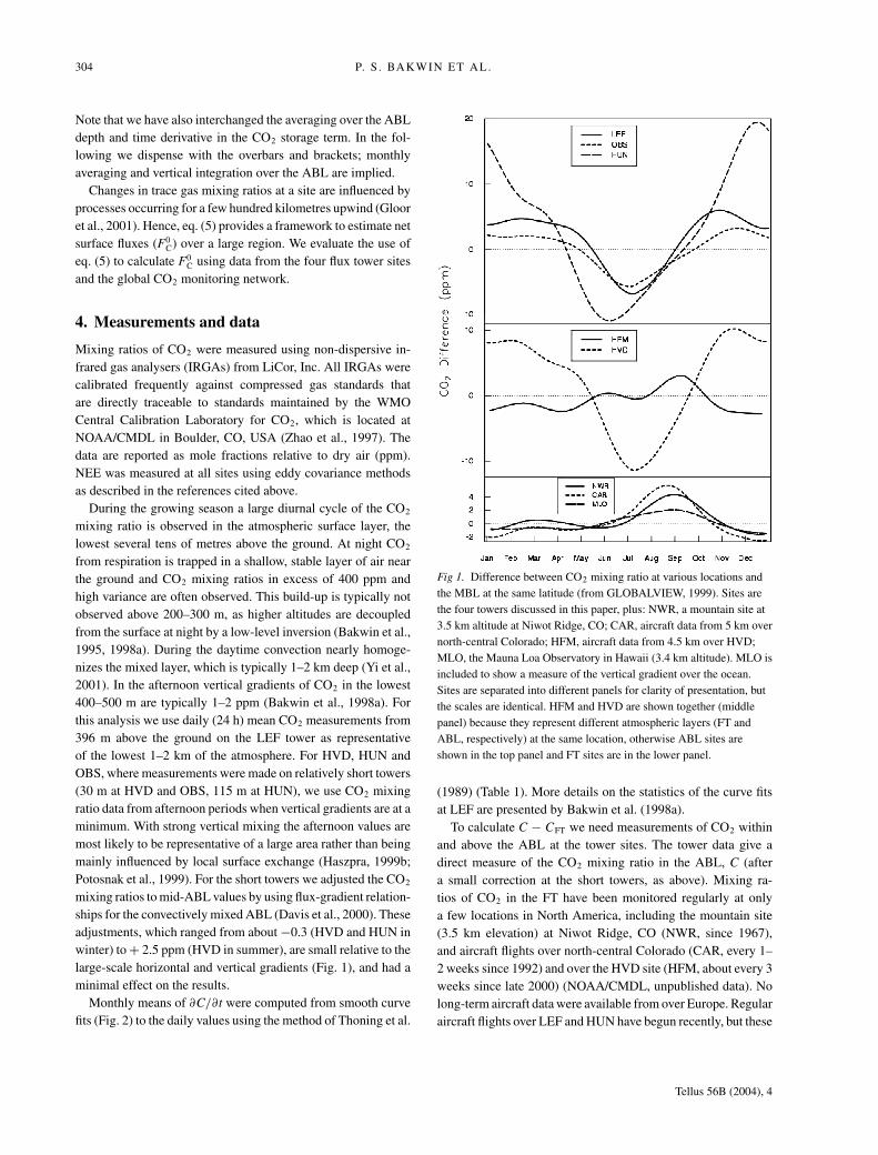
mixing ratios to mid-ABL values by using flux-gradient relation-ships for the convectively mixed ABL (Davis et al., 2000). Theseadjustments, which ranged from about −0.3 (HVD and HUN inwinter) to + 2.5 ppm (HVD in summer), are small relative to thelarge-scale horizontal and vertical gradients (Fig. 1), and had aminimal effect on the results.

Monthly means of ∂C/∂t were computed from smooth curvefits (Fig. 2) to the daily values using the method of Thoning et al.

Fig 1. Difference between CO2 mixing ratio at various locations andthe MBL at the same latitude (from GLOBALVIEW, 1999). Sites arethe four towers discussed in this paper, plus: NWR, a mountain site at3.5 km altitude at Niwot Ridge, CO; CAR, aircraft data from 5 km overnorth-central Colorado; HFM, aircraft data from 4.5 km over HVD;MLO, the Mauna Loa Observatory in Hawaii (3.4 km altitude). MLO isincluded to show a measure of the vertical gradient over the ocean.Sites are separated into different panels for clarity of presentation, butthe scales are identical. HFM and HVD are shown together (middlepanel) because they represent different atmospheric layers (FT andABL, respectively) at the same location, otherwise ABL sites areshown in the top panel and FT sites are in the lower panel.

(1989) (Table 1). More details on the statistics of the curve fitsat LEF are presented by Bakwin et al. (1998a).

To calculate C − CFT we need measurements of CO2 withinand above the ABL at the tower sites. The tower data give adirect measure of the CO2 mixing ratio in the ABL, C (aftera small correction at the short towers, as above). Mixing ra-tios of CO2 in the FT have been monitored regularly at onlya few locations in North America, including the mountain site(3.5 km elevation) at Niwot Ridge, CO (NWR, since 1967),and aircraft flights over north-central Colorado (CAR, every 1–2 weeks since 1992) and over the HVD site (HFM, about every 3weeks since late 2000) (NOAA/CMDL, unpublished data). Nolong-term aircraft data were available from over Europe. Regularaircraft flights over LEF and HUN have begun recently, but these

Tellus 56B (2004), 4


Fig 2. Mixing ratios and NEE of CO2 at (a)OBS, (b) HUN, (c) LEF and (d) HVD. Datafor OBS, HVD and LEF are for 1997, whileHUN data are a composite from 1998 and1999. CO2 mixing ratios at HUN have beenadjusted to account for the NorthernHemisphere mean rate of increase of CO2 inorder to be comparable to the other sites.Daily measurements of CO2 mixing ratioshave been fitted with a smooth curve (thickblack line) after the method of Thoning et al.(1989). Grey lines are local NEE data (towereddy fluxes) that have been smoothed with arunning mean filter with a 5-day timeconstant for the purposes of illustration.Positive NEE values indicate that thevegetation is a source of CO2 to theatmosphere. The thin lines represent CO2

mixing ratios in the MBL at the latitudes ofthe tower sites (GLOBALVIEW, 1999).Scales for each tower are identical.

Table 1. Monthly values of terms in eq. (3) at LEF (1997), and localNEE from the tower eddy fluxes. Units are µmol m−2 s−1

Month wM(C − CFT) zi∂C/∂t F0C NEE

Jan 1.1 0.0 1.1 0.4Feb 0.8 0.0 0.9 0.4Mar 1.2 0.0 1.2 0.4Apr 0.6 0.0 0.6 0.3May 0.2 −0.2 0.1 0.2Jun −1.0 −0.3 −1.2 −1.2Jul −1.9 −0.2 −2.1 −1.7Aug −1.2 0.1 −1.1 −1.0Sep 0.3 0.2 0.5 0.4Oct 1.1 0.1 1.2 1.3Nov 0.9 0.0 0.9 0.6Dec 0.4 0.0 0.4 0.4

data sets are still too short for our present purposes. Gradientsof CO2 between the MBL and the continental FT are generallysomewhat smaller than those between the MBL and the conti-nental ABL (Fig. 1). Hence, lacking direct measurements of CFT

over the towers during 1997 (LEF, HVD, OBS) and 1998–1999(HUN), we use as proxies data from the MBL at the latitude ofeach tower and alternatively from 5 km altitude at CAR. Com-parison of results using these two data sets to estimate CFT overthe towers gives an idea of the uncertainty introduced into thecalculation of F0

C. The MBL reference includes data from sites inboth the Atlantic and Pacific Ocean basins, but monthly mean At-lantic and Pacific data at the same latitude typically differ by lessthan 1 ppm (P. Tans, NOAA/CMDL, personal communication,2002).

Helliker et al. (2003) also recognized the importance of verti-cal advection in the budget of CO2 in the ABL. They used datafrom our Wisconsin tower site (LEF), and estimated vertical ad-vection by analysis of the budget of water vapour in the ABL withthe surface flux of water vapour measured by eddy covariance.As in our analysis, Helliker et al. (2003) used the MBL data toestimate CFT. Helliker et al. (2003) compared vertical exchangederived using water vapour observations with those derived fromreanalysis, and showed that these are similar in fair weather con-ditions but that the Reanalysis-derived exchange velocity is sub-stantially smaller than that derived using a water vapour budget.

Tellus 56B (2004), 4


Their work was the first to show that very reasonable estimatesof the surface flux of CO2 could be obtained by this method forthe region around LEF, indicating that a quantitative estimateof the vertical exchange term can be obtained from simple dataand that vertical exchange is probably dominant over horizontal.Our analysis differs from that of Helliker et al. (2003) in severalimportant ways: (1) our estimates of w are taken from the Re-analysis data; (2) we include the ∂C/∂t term; (3) we analyse datafrom three additional tower sites; and (4) Helliker et al. (2003)did not consider the influence of anthropogenic CO2 emissionson FC, as compared to NEE.

For each tower site we estimate wM as the monthly mean of theabsolute value of daily vertical velocity from the NCEP Reanal-ysis product (Kalnay et al., 1996), which we have interpolated tothe height of the ABL top (zi) and converted from pressure coor-dinates (Pa s−1). Resolved vertical velocity in the NCEP modelbalances horizontal divergence, and represents a grid-cell (about200 × 200 km) average value. The model parametrizes the ma-jor physical processes involving vertical motions, including deepand shallow convection, large-scale precipitation, gravity wavedrag, radiation and radiative effects of clouds, boundary layerdynamics, surface hydrology and vertical and horizontal diffu-sion. Subgrid convective mixing is simulated but is not includedin the grid-cell mean vertical velocity.

Yi et al. (2001) estimated zi at LEF using measurementsfrom an ABL radar system. The measurements were made dur-ing March–November 1998 and zi was estimated for the win-ter months by using an empirical fit to the surface buoyancyflux. Monthly mean values of zi varied from 1.0 km in winter(November–February) to 2.0 km in May. Haszpra (1999a) esti-mated the monthly mean (1987–1992) of zi for a suburban sitenear Budapest, Hungary. Mean afternoon zi ranged from 0.6 kmin winter to 1.5 km in summer. Mixed layer depths at HUN areexpected to be very similar. Radiosondes were used to measurezi at OBS frequently during three intensive field campaigns aspart of the BOREAS Project in May–September 1994 (Barr andBetts, 1997). The BOREAS data show zi values and seasonalchanges that are very similar to the LEF observations. We lackdirect observations of zi at HVD. For the present work we usethe monthly mean of measurements of zi from LEF in 1998 (Yiet al., 2001) for LEF, HVD and OBS, and for HUN we use theBudapest data (Haszpra, 1999a). Values of zi ∂C/∂t are gener-ally small compared with wM(C − CFT) (Table 1). Values ofwM from NCEP also depend on altitude, typically decreasing by15–30% from the 700 mbar to 850 mbar, while zi is usually inthe range of 760–860 mbar at our sites. Hence, our estimates ofF0

C depend on zi only weakly.Since ABL convection is forced by the surface buoyancy flux,

zi exhibits a seasonal cycle with a maximum in spring and min-imum in winter (Stull, 1988; Yi et al., 2001). Of course, zi alsovaries with the weather conditions. Using a trajectory modelMoody et al. (1998) estimated that zi averaged for different syn-optic classifications at HVD varied by a factor of two (875 to

1780 m), but for classes representing 63% of all occurrencesaverage zi was very consistent in the range of 1200–1250 m.

It is likely that F0C and zi are correlated on synoptic time scales,

which would require an additional term in eq. (5). For example,in summer the passage of a synoptic disturbance can temporarilyincrease the mixing depth, often to near the depth of the tropo-sphere, while net uptake by the vegetation is suppressed due tocloudy conditions. During disturbed weather the radar systemis often unable to unambiguously determine zi, which may bepoorly defined. Without a means to estimate zi for all time pe-riods we cannot evaluate the magnitude of this covariance. As arough estimate let us assume that in summer zi equals 2 km and10 km during fair and disturbed weather, respectively, and F0

C

equals −3 and −1 µmol m−2 s−1 as a 24 h mean during theseconditions. If fair and disturbed conditions occur with equal fre-quency then there is a covariance term of +0.5 µmol m−2 s−1,roughly half the magnitude of the value of wM(C − CFT) in sum-mer (Table 1). The true covariance will almost certainly be muchsmaller than this since disturbed conditions occur for less thanhalf the time and since F0

C and zi are not perfectly correlated. Inwinter the biogenic component of F0

C (mainly soil respiration)responds weakly to synoptic conditions since soil temperatureschange relatively slowly. Hence, using monthly mean values ofF0

C and zi is a reasonable first approximation.

5. Results

At LEF, HVD and HUN ABL CO2 mixing ratios and local sur-face fluxes are out of phase: CO2 mixing ratios start to decreaserapidly in spring about 20–30 days before the vegetation beginstaking up CO2 in net, and similarly CO2 increases in the autumn1–2 months before the forest becomes a net source for CO2 to theatmosphere (Fig. 2). These patterns indicate that advection playsa role in the budget of ABL CO2 at these sites, at least duringspring and autumn. At OBS NEE is more closely in phase withCO2 mixing ratios, and NEE values are much smaller than at theother sites.

Equation (5) allows us to use CO2 mixing ratio measurementsfrom tower sites to estimate the regional surface flux of CO2, F0

C,which includes both biotic exchange and anthropogenic emis-sions. The results represent an estimate of the net surface ex-change on a regional spatial scale, i.e. ∼106 km2. At LEF andHUN F0

C is in reasonable accord with the local scale flux mea-sured by eddy covariance (NEE) during the spring, summer andautumn seasons (Figs 3b and c). Though the spatial scales rep-resented by these two flux estimates are very different there isreason to expect that eddy flux data from the LEF and HUN tow-ers should be fairly representative of the larger regions. Theseresults give some confidence that the regional flux estimates arereasonable. At OBS in summer the regional flux (F0

C) indicatesmuch more uptake by the vegetation than the local NEE (Fig. 3a),while at HVD F0

C indicates somewhat less summertime uptakethan the local NEE (Fig. 3d). These results are in agreement with

Tellus 56B (2004), 4


Fig 3. Regional CO2 flux estimates calculated as described in the text (lines), and local fluxes measured at the towers by eddy covariance methods(×): (a) OBS, (b) HUN, (c) LEF and (d) HVD. CO2 in the free troposphere over the towers was estimated either from MBL data (black line) oraircraft data from 5 km over Colorado (CAR, grey line). Thin horizontal lines indicate inventory estimates of fossil fuel emissions of CO2 for theregions indicated. At OBS the calculation was repeated with wintertime (November–March) C values reduced by 1.6 ppm to accountapproximately for pollution from thousands of kilometres distant (dotted line, see text).

expectations. The regional landscape around OBS is a patchworkof forest stands of varying ages, with fire as the main disturbance,and the stand in the immediate vicinity of the tower is relativelyold, having last burned about 120 yr ago. Younger stands aremore productive (Litvak et al., 2003), and our regional flux esti-mate probably reflects the influence of these younger stands ona large spatial scale. Similarly, the vegetation in the immediatevicinity of HVD is a protected and managed aggrading hard-wood forest, while the surrounding area includes less productiveforests, agricultural fields and human developments, all of whichare likely to take up less carbon during the growing season.

Figure 3 shows a single year of data for each tower, but exam-ination of other years for LEF, HVD and OBS gave very similarresults (only one full year of NEE data was available from HUN).

Our regional flux estimates are consistently much greater thanlocal NEE at all the towers in winter (Fig. 3). It is likely that emis-sions of CO2 from fossil-fuel combustion within the larger areaof the regional estimates contribute to this discrepancy. The tow-ers are located to minimize the contribution of anthropogenicemissions on measurements of NEE. To estimate the magni-

tude of the anthropogenic CO2 flux that contributes to F0C we

used measurements of CO and SF6. Carbon monoxide is emit-ted during burning, and CO/CO2 emission ratios are reasonablywell known for industrialized areas. To estimate anthropogenicemissions of CO2 from CO data we used an emissions ratio of20 parts per billion (ppb) of CO per ppm of CO2, which is ap-propriate for North America and Western Europe (Bakwin et al.,1998b). There are no known natural sources of SF6, which isused primarily as a dielectric insulator for industrial applica-tions. Hence, SF6 is a good tracer for industrial activities. Wecalculated a CO2/SF6 emissions ratio of 15.3 ppm/ppt (partsper trillion) from global emissions inventories. Several trace gasspecies including CO and SF6 are measured in flask samplescollected weekly at all sites of the NOAA/CMDL CooperativeAir Sampling Network, which includes LEF and HUN. At HVDCO was measured using a continuous, in situ analyser (J. W.Munger, Harvard University, unpublished data), but SF6 was notmeasured. No SF6 or CO data were available from OBS.

Regional estimates of the anthropogenic flux of CO2 werecalculated from SF6 and CO using eq. (5) and using MBL data

Tellus 56B (2004), 4


Fig 4. Regional fossil fuel flux of CO2 estimated from CO and SF6 data using the methods described in the text. Measurements of SF6 at HUN (a)and LEF (b) were started in mid-1997. Data are averaged for 1998–2001 for HUN and LEF and for 1996–2001 for HVD (c), and error bars show onestandard deviation of the mean across years. Annual mean fossil fuel emissions from inventory estimates (dashed horizontal lines) have beencalculated for the regions indicated by multiplying the human population density by the national per capita emissions (Marland et al., 2002).

for these species from the NOAA/CMDL network (unpublisheddata). The method is identical to that used to compute CO2 fluxes,F0

C, and the results should be representative of the same regionsas those for CO2.

At HUN and LEF anthropogenic CO2 fluxes calculated us-ing CO and SF6 are in good agreement, and agree fairly wellwith inventory estimates from these regions (Figs 4a and b). Theanthropogenic flux calculated from CO at HUN shows a fairlystrong seasonal cycle, with higher emissions in winter than sum-mer. Anthropogenic emissions of CO2 in Europe are expected toexhibit a similar seasonal cycle (Levin et al., 1995). Emissions ofSF6 are not known to be seasonal, so anthropogenic CO2 emis-sions calculated from SF6 would not be expected to be seasonal.Anthropogenic emissions of CO2 are also seasonal in the USA,with higher fluxes in winter than summer (G. Marland, personalcommunication, 2003), but seasonal patterns calculated from COat LEF and HVD are complex. In summertime it is likely thatoxidation of biogenic hydrocarbons such as isoprene contributesto the abundance of CO at these towers (Potosnak et al., 1999),but this source is not considered in our analysis. Seasonal differ-ences in transport may also contribute to the seasonal pattern of

calculated anthropogenic fluxes, but examination of these sea-sonal changes is outside the scope of our simple one-dimensionalanalysis.

Our estimates of the anthropogenic CO2 flux at HUN are ingood agreement with the inventory estimate for Hungary andAustria (Fig. 4a). Other areas of Western Europe exhibit simi-lar flux densities. At LEF our estimates based on CO and SF6

are about half of the inventory value for the states of Wisconsinand Minnesota (Fig. 4b). The area influencing these calculationsmay be substantially larger than this, and regions farther fromthe tower in the prevailing westerly wind direction are gener-ally of lower population density. For example, the populationdensities of North and South Dakota are 10–15% of those ofWisconsin and Minnesota. The calculated flux at HVD is alsosubstantially lower than the inventory estimate for the Northeast-ern USA (New York and the New England states) (Fig. 4c), againsuggesting that the area of influence for the tower mixing ratiodata is substantially larger than this densely populated region.

We have no CO or SF6 data from OBS. The region for severalhundred kilometres around the tower is very sparsely populated.However, data from other high latitude sites in Canada indicate

Tellus 56B (2004), 4


that pollutants are elevated in the continental ABL in winter dueto long-range transport from Europe and Asia. At both Alert(82.5◦N, 62.5◦W) and Fraserdale (49.9◦N, 81.6◦W) CH4 is en-hanced in winter by about 25 ppb relative to the high-latitudeMBL (Worthy et al., 1998). Using a CH4/CO2 emissions ratioof 16 ppb/ppm from the AGASP III programme (Conway et al.,1993), this translates to an excess of 1.6 ppm of CO2 in thecontinental ABL over Canada in winter and represents a contri-bution to the gradient of CO2 that results from fluxes thousandsof kilometres upwind of the tower. Subtracting this amount from(C−CFT) at OBS gives results in reasonable agreement with thetower NEE in winter (Fig. 3a).

The magnitudes of our estimates of anthropogenic contribu-tions to the regional CO2 fluxes are in fair accord with thosewhich are needed to explain the wintertime differences betweenF0

C and NEE at these sites (Fig. 3). Fossil-fuel emissions alsoaffect our regional flux estimates in summer, especially at HVDwhich is in an area of particularly high fossil-fuel emissionsdensity (Fig. 3d). In these temperate areas fossil-fuel fluxes arebelieved to be substantially higher in winter than summer (Levinet al., 1995; G. Marland, personal communication, 2003).

6. Discussion

Our budget analysis indicates that it is feasible to measure F0C

on a regional scale (i.e. ∼106 km2) by using measurements ofCO2 mixing ratios if horizontal and vertical advection can beestimated. The parametrization represented by eq. (2) is neces-sarily rough because at present sufficient data do not exist toenable a more accurate representation of horizontal and verti-cal advective exchange. This could be accomplished by usinga mesoscale network of tower and aircraft sites at which CO2

mixing ratios are accurately measured, and interpreting of thedata with a trajectory model. The spacing of such a tower net-work should be of the order of several hundred kilometres, theapproximate length scale represented by trace gas mixing ra-tio measurements (Gloor et al., 2001). Frequent vertical profilesover the towers using small aircraft would define the verticalmixing ratio difference between the ABL and FT. The trajectorymodel would provide observationally based estimates of windvector (U and w in eq. 1), zi and other parameters important forestimation of surface fluxes. An early study of this type, thoughmainly using data from a research aircraft campaign, has beenpresented by Gerbig et al. (2003).

Though data from very tall transmitter towers are least af-fected by very local surface exchange processes, our data forHVD, HUN and OBS indicate that properly selected measure-ments on short (30–115 m) towers also reflects regional scaleprocesses. Small (0–2 ppm) daytime vertical gradients from thesurface layer to the mid-ABL can be adequately estimated if sur-face exchange data are available (Potosnak et al., 1999; Daviset al., 2000), and these gradients are fairly small relative tothe CO2 difference across the top of the ABL, and to day-to-

day changes in CO2 that are associated mainly with synopticvariability.

The strategy outlined here also provides a means to assessregional anthropogenic fluxes of CO2 by using specific tracerssuch as CO and SF6. Hence, these tracers should be measuredin any future tower and aircraft network and calibrations shouldbe carefully tied to internationally accepted standards. Measure-ments of other tracers may provide greater specificity to partic-ular anthropogenic processes.

Though there are dozens of towers worldwide where NEE isbeing measured, at only a very few of these sites are measure-ments of CO2 mixing ratios traceable to the globally acceptedWMO mole fraction scale. A relatively small increase in effortis required to calibrate CO2 measurements adequately. Such aneffort would yield an abundance of CO2 mixing ratio data overcontinental areas that would be extremely useful to constrainestimates of regional net atmosphere/biosphere exchange ofCO2.

7. Acknowledgments

This research was funded in part by the National Institute forGlobal Environmental Change through the US Department ofEnergy (DoE) through grants to Harvard University and the Uni-versity of Colorado. Any opinions, finding and conclusions orrecommendations herein are those of the authors and do notnecessarily reflect the views of the DoE. The carbon dioxidemixing ratio measurements, and site infrastructure and mainte-nance at LEF, were supported by the Atmospheric ChemistryProject of the Climate and Global Change Program of the Na-tional Oceanic and Atmospheric Administration. Measurementsin Hungary were supported by the US–Hungarian Scientific andTechnological Joint Fund (J.F. 504 (1996–1999)) and by theHungarian National Scientific Research Fund (OTKA T23811(1997–2000) and OTKA T32440 (2000–2003)), and by the Eu-ropean Union (CarboEurope AEROCARB, contract no EVK2-CT-1999-00013). Work at the LEF television tower would notbe possible without the gracious cooperation of the WisconsinEducational Communications Board and R. Strand, chief engi-neer for WLEF-TV. Use of the tower and transmitter building atthe site in Hungary was kindly provided by Antenna HungariaCorporation. We thank A. S. Denning (Colorado State Uni-versity) and P. P. Tans for their comments on a draft of thispaper.

References

Bakwin, P. S., Tans, P. P., Hurst, D. F. and Zhao, C. 1998a. Measurementsof carbon dioxide on very tall towers: results of the NOAA/CMDLprogram. Tellus 50B, 401–415.

Bakwin, P. S., Tans, P. P. White, J. W. C. and Andres, R. J. 1998b.Determination of the isotopic (13C/12C) discrimination by terrestrialbiology from a global network of observations. Global Biogeochem.Cycles 12, 555–562.

Tellus 56B (2004), 4


Bakwin, P. S., Zhao, C., Ussler, W. III, Tans, P. P. and Quesnell, E. 1995.Measurements of carbon dioxide on a very tall tower. Tellus 47B,535–549.

Baldocchi, D., Falge, E., Gu, L., Olson, R., Hollinger, D. et al. 2001.FLUXNET: a new tool to study the temporal and spatial variability ofecosystem-scale carbon dioxide, water vapor and energy flux densities.Bull. Am. Meteorol. Soc. 82, 2415–2434.

Barford, C. C., Wofsy, S. C., Goulden, M. L., Munger, J. W., Pyle, E. H.et al. 2001. Factors controlling long- and short-term sequestration ofatmospheric CO2 in a mid-latitude forest. Science 294, 1688–1691.

Barr, A. G. and Betts, A. K. 1997. Radiosonde boundary layer budgetsabove a boreal forest. J. Geophys. Res. 102, 29 205–29 212.

Battle, M., Bender, M., Tans, P. P., White, J. W. C., Ellis, J. T. et al. 2000.Global carbon sinks and their variability, inferred from atmosphericO2 and δ13C. Science 287, 2467–2470.

Bousquet, P., Peylin, P., Ciais, P., Le Quere, C., Friedlingstein, P. et al.2000. Regional changes in carbon dioxide fluxes of land and oceanssince 1980. Science 290, 1342–1346.

Chou, W. W., Wofsy, S. C., Harriss, R. C., Lin, J. C., Gerbig, C. et al. 2002.Net fluxes of CO2 in Amazonia derived from aircraft observations. J.Geophys. Res. 107(D22), 4614, doi:10.1029/2001JD001295.

Ciais, P., Tans, P. P. and Trolier, M. 1995. A large northern-hemisphereterrestrial CO2 sink indicated by the 13C/12C ratio of atmosphericCO2. Science 269, 1098–1102.

Conway, T. J., Steele, L. P. and Novelli, P. C. 1993. Correlations amongatmospheric CO2, CH4 and CO in the Arctic, March 1989. Atmos.Environ. 27A, 2881–2894.

Conway, T. J., Tans, P. P., Waterman, L. S., Thoning, K. W., Kitzis, D.R. et al. 1994. Evidence for interannual variability of the carbon cyclefrom the National Oceanic and Atmospheric Administration/ClimateMonitoring and Diagnostics Laboratory global air sampling network.J. Geophys. Res. 99, 22 831–22 856.

Davis, K. J., Bakwin, P. S., Yi, C., Berger, B. W., Zhao, C. et al. 2003. Theannual cycles of CO2 and H2O exchange over a northern mixed forestas observed from a very tall tower. Global Change Biol. 9, 1278–1293.

Davis, K. J., Yi, C., Berger, B. W., Kubesh, R. J. and Bakwin, P. S.2000. Scalar budgets in the continental boundary layer. In: Proceed-ings of the 14th Symposium on Boundary Layer and Turbulence,7–11 August, American Meteorological Society, Aspen, CO, 100–103.

Fan, S.-M., Gloor, M., Mahlman, J., Pacala, S., Sarmiento, J. L. et al.1998. A large terrestrial carbon sink in North America implied byatmospheric and oceanic CO2 data and models. Science 282, 442–446.

Gerbig, C., Lin, J. C., Wofsy, S. C., Daube, B. C., Andrews, A. E. et al.2003. Toward constraining regional-scale fluxes of CO2 with atmo-spheric observations over a continent: 2. Analysis of COBRA datausing a receptor-oriented framework. J. Geophys. Res. 108, 4757,doi:10.1029/2003JD003770.

GLOBALVIEW 1999. Cooperative Atmospheric Data IntegrationProject—Carbon Dioxide, CD-ROM. NOAA/CMDL, Boulder,CO. (Also available on the Internet via anonymous FTP toftp.cmdl.noaa.gov, Path: ccg/co2/GLOBALVIEW).

Gloor, M., Bakwin, P., Tans, P., Hurst, D., Lock, L. et al. 2001. Whatis the concentration footprint of a tall tower? J. Geophys. Res. 106,17 831–17 840.

Gloor, M., Fan, S., Sarmiento, J. and Pacala, S. 2000. Optimal samplingof the atmosphere for purpose of inverse modeling: a model study.Global Biogeochem. Cycles 14, 407–428.

Goulden, M. L., Munger, J. W., Fan, S.-M., Daube, B. C. and Wofsy, S. C.1996a. Measurements of carbon sequestration by long-term eddy co-variance: methods and a critical evaluation of accuracy. Global ChangeBiol. 2, 169–182.

Goulden, M. L., Munger, J. W., Fan, S.-M., Daube, B. C. and Wofsy, S.C. 1996b. Exchange of carbon dioxide by a deciduous forest: responseto interannual climate variability. Science 271, 1576–1578.

Goulden, M. L., Wofsy, S. C., Harden, J. W., Trumbore, S. E., Crill, P.M. et al. 1998. Sensitivity of boreal forest carbon balance to soil thaw.Science 279, 214–217.

Gurney, K. R., Law, R. M., Denning, A. S., Rayner, P. J., Baker, D. et al.2002. Towards robust regional estimates of CO2 sources and sinksusing atmospheric transport models. Nature 415, 626–630.

Haszpra, L. 1999a. Measurements of atmospheric carbon dioxide at alow elevation rural site in Central Europe. Idojaras 103, 93–105.

Haszpra, L. 1999b. On the representativeness of carbon dioxide mea-surements. J. Geophys. Res. 104, 26 953–26 960.

Haszpra, L., Barcza, Z., Bakwin, P. S., Berger, B. W., Davis, K. J.et al. 2001. Measuring system for the long-term monitoring of bio-sphere/atmosphere exchange of carbon dioxide. J. Geophys. Res. 106,3057–3069.

Helliker, B., Berry, J., Betts, A., Davis, K. and Bakwin, P. 2003. Es-timates of ABL-scale net carbon dioxide flux in Central Wisconsin.EOS, Trans. Am. Geophys. Un. 84(46), Fall Meet. Suppl., AbstractB42B-01.

Houghton, R. A. 1999. The annual net flux of carbon to the atmospherefrom changes in land use 1850–1990. Tellus 51B, 298–313.

Hurwitz, M. D., Ricciuto, D. M., Davis, K. J., Wang, W., Yi, C. et al.2004. Advection of carbon dioxide in the presence of storm systemsover a northern Wisconsin forest. J. Atmos. Sci. 61, 607–618.

Kalnay, E., Kanamitsu, M., Kistler, R., Collins, W., Deaven, D. et al.1996. The NCEP/NCAR 40-year reanalysis project. Bull. Am. Mete-orol. Soc. 77, 437–471.

Keeling, R. F., Piper, S. C. and Heimann, M. 1996. Global and hemi-spheric CO2 sinks deduced from changes in atmospheric O2 concen-tration. Nature 381, 218–221.

Leith, H. 1963. The role of vegetation in the carbon dioxide content ofthe atmosphere. J. Geophys. Res. 68, 3887–3898.

Levin, I., Graul, R. and Trivett, N. B. A. 1995. Long-term observations ofatmospheric CO2 and carbon isotopes at continental sites in Germany.Tellus 47B, 23–34.

Litvak, M., Miller, S., Wofsy, S. C. and Goulden, M. 2003. Effect ofstand age on whole ecosystem CO2 exchange in the Canadian borealforest. J. Geophys. Res. 108 doi:10.1029/2001JD000854, 29 January2003.

Mackay, D. S., Ahl, D. E., Ewers, B. E., Gower, S. T., Burrows, S. N. et al.2002. Effects of aggregated classifications of forest composition onestimates of evapotranspiration in a northern Wisconsin forest. GlobalChange Biol. 8, 1253–1266.

Marland, G., Boden, T. A. and Andres, R. J. 2002. Global, regionaland national fossil fuel CO2 emissions. In: Trends: a Compendiumof Data on Global Change. Carbon Dioxide Information AnalysisCenter, Oak Ridge National Laboratory, US Department of Energy,Oak Ridge, TN.

Tellus 56B (2004), 4


Moody, J. L., Munger, J. W., Goldstein, A. H., Jacob, D. J. and Wofsy,S. C. 1998. Harvard Forest regional-scale air mass composition byPatterns in Atmospheric Transport History (PATH). J. Geophys. Res.103, 13 181–13 194.

Myneni, R. B., Keeling, C. D., Tucker, C. J., Asrar, G. and Nemani, R.R. 1997. Increased plant growth in northern high latitudes from 1981to 1991. Nature 386, 145–148.

Pacala, S. W., Hurtt, G. C., Baker, D., Peylin, P., Houghton, R. A. et al.2001. Consistent land- and atmosphere-based U.S. carbon sink esti-mates. Science 292, 2316–2320.

Potosnak, M. J., Wofsy, S. C., Denning, A. S., Conway, T. J., Munger, J.W. et al. 1999. Influence of biotic exchange and combustion sources onatmospheric CO2 concentrations in New England from observationson a forest flux tower. J. Geophys. Res. 104, 9561–9569.

Randerson, J. T., Field, C. B., Fung, I. Y. and Tans, P. P. 1999. Increases inearly season ecosystem uptake explain recent changes in the seasonalcycle of atmospheric CO2. Geophys. Res. Lett. 26, 493–496.

Rayner, P. J., Enting, I. G., Francey, R. J. and Langenfields, R. 1999.Reconstructing the recent carbon cycle from atmospheric CO2, δ13Cand O2/N2 observations. Tellus 51B, 213–232.

Rayner, P. J., Enting, I. G. and Trudinger, C. M. 1996. Optimizing theCO2 observing network for constraining sources and sinks. Tellus48B, 433–444.

Running, S. W., Gower, S. T., Bakwin, P. S., Hibbard, K. A., Baldocchi,D. D. et al. 1999. A global terrestrial monitoring network integratingtower fluxes, flask sampling, ecosystem modeling and EOS satellitedata. Remote Sensing Environ. 70, 108–127.

Stull, R. B. 1988. An Introduction to Boundary Layer Meteorology.Kluwer Academic Publishers, Dordrecht.

Tans, P. P., Bakwin, P. S. and Guenther, D. W. 1996. A feasible globalcarbon cycle observing system: a plan to decipher today’s carbon cyclebased on observations. Global Change Biol. 2, 309–318.

Tans, P. P., Fung, I. Y. and Takahashi, T. 1990. Observational con-straints on the global atmospheric CO2 budget. Science 247, 1431–1438.

Thoning, K. W., Tans, P. P. and Komhyr, W. D. 1989. Atmospheric carbondioxide at Mauna Loa Observatory, 2, Analysis of the NOAA GMCCdata, 1974–1985. J. Geophys. Res. 94, 8549–8565.

Valentini, R., Matteucci, G., Dolman, A. J., Schulze, E.-D., Rebmann,C. et al. 2000. Respiration as the main determinant of carbon balancein European forests. Nature 404, 861–865.

Wofsy, S. C., Goulden, M. L., Munger, J. W., Fan, S.-M., Bakwin, P.S. et al. 1993. Net exchange of CO2 in a mid-latitude forest. Science260, 1314–1317.

Wofsy, S. C. and Harriss, R. C. 2002. The North American CarbonProgram (NACP). Report to the Interagency Working Group of the USGlobal Change Research Program. National Center for AtmosphericResearch, Boulder, CO, USA. http://www.esig.ucar.edu/nacp/

Worthy, D. E. J., Levin, I., Trivett, N. B. A., Kuhlmann, A. J., Hopper,J. F. et al. 1998. Seven years of continuous methane observations at aremote boreal site in Ontario, Canada. J. Geophys. Res. 103, 15 995–16 007.

Yi, C., Davis, K. J., Bakwin, P. S. and Berger, B. W. 2001. Long-termobservations of the evolution of the planetary boundary layer. J. Atmos.Sci. 58, 1288–1299.

Zhao, C. L., Tans, P. P. and Thoning, K. W. 1997. A high precisionmanometric system for absolute calibrations of CO2 in dry air. J.Geophys. Res. 102, 5885–5894.

Tellus 56B (2004), 4

Regional carbon dioxide fluxes from mixing ratio data

Documents

Transcript of Regional carbon dioxide fluxes from mixing ratio data