Tropical storm-induced near-inertial internal waves during the Cirene experiment: Energy fluxes and...

Tropical storm-induced near-inertial internal waves during theCirene experiment: Energy fluxes and impact on vertical mixing

Y. Cuypers,1 X. Le Vaillant,1 P. Bouruet-Aubertot,1 J. Vialard,1 and M. J. McPhaden2

Received 9 January 2012; revised 22 November 2012; accepted 7 December 2012.

[1] Near-inertial internal waves (NIW) excited by storms and cyclones play an essentialrole in driving turbulent mixing in the thermocline and interior ocean. Storm-inducedmixing may be climatically relevant in regions like the thermocline ridge in thesouthwestern Indian Ocean, where a shallow thermocline and strong high frequency windactivity enhance the impact of internal gravity wave-induced mixing on sea surfacetemperature. The Cirene research cruise in early 2007 collected ship-borne and mooringvertical profiles in this region under the effect of a developing tropical cyclone. In thispaper, we characterize the NIW field and the impact of these waves on turbulent mixing inthe upper ocean. NIW packets were identified down to 1000m, the maximum depth of themeasurements. We estimated an NIW vertical energy flux of up to 2.5mWm�2 within thepycnocline, which represents about 10% of the maximum local wind power input. Anon-negligible fraction of the wind power input is hence potentially available for subsurfacemixing. The impact of mixing by internal waves on the upper ocean heat budget wasestimated from a fine-scale mixing parameterization. During the first leg of the cruise(characterized by little NIW activity), the average heating rate due to mixing was~0.06 �Cmonth�1 in the thermocline (23–24 kgm�3 isopycnals). During the second leg,characterized by strong NIW energy in the thermocline and below, this heating rate increasedto 0.42 �Cmonth�1, indicative of increased shear instability along near inertial waveenergy pathways.

Citation: Cuypers, Y., X. Le Vaillant, P. Bouruet-Aubertot, J. Vialard, and M. J. McPhaden (2013), Tropical storm-induced near-inertial internal waves during the Cirene experiment: Energy fluxes and impact on vertical mixing,J. Geophys. Res. Oceans, 118, doi:10.1029/2012JC007881.

1. Introduction

[2] Internal wave breaking is one of the main processesinducing turbulent mixing in the stratified ocean. The impor-tance of this process for determining large-scale patterns ofocean circulation (like the meridional overturning circulation)has been highlighted in numerous studies [e.g., Marotzkeand Scott, 1999; Wunsch and Ferrari, 2004]. There is alsoevidence that near-surface mixing can have a considerableclimatic influence in regions where the sea surface temperatureis high and sustains deep atmospheric convection [e.g., Koch-Larrouy et al., 2008]. This underlines the requirement for amore comprehensive understanding of energy pathways from

large scales to mixing scales and especially of the lifecycleof internal waves from generation to breaking.[3] The two main sources of internal gravity waves are

tides and high frequency atmospheric forcing [Munk andWunsch, 1998; Wunsch, 1998]. The strong wind and windvector rotation associated with tropical cyclones induce anenergetic inertial current response. To the right of the cyclonetrack (in the Northern Hemisphere), this results in intensekinetic energy generation in the upper ocean, because windstress vectors rotate in the same direction as storm-generatedoceanic currents, maximizing power input to the surfaceocean [e.g., Price, 1981] and wind stress is larger on the rightside of the storm track, partly due to the storm translationspeed [Chang and Anthes, 1978]. In the SouthernHemisphere, strong inertial currents and enhanced mixingoccur on the left side of the storm track. A large fraction ofthis kinetic energy is consumed by vertically mixing warmsurface water down into the thermocline [Jaimes and Shay,2009]. But a fraction of this energy input radiates down inthe interior ocean under the form of near-inertial internalwaves (hereafter NIW). There is a need to evaluate the frac-tion of the cyclone-generated kinetic energy that penetratesin the interior ocean. This is important for understandingthe cyclone response (the cyclone-induced surface coolingwill be more intense if most of the energy is consumed

1Laboratoire d’Océanographie Expérimentation et Approches Numériques,CNRS, UPMC, IRD, Paris, France.

2Pacific Marine Environmental Laboratory, NOAA, Seattle, Washington,USA.

Corresponding author: Y. Cuypers, LOCEAN – Case 100, UniversitéPierre et Marie Curie, 75232 Paris CEDEX 05, France. ([email protected])

©2012. American Geophysical Union. All Rights Reserved.2169-9275/13/2012JC007881

1

JOURNAL OF GEOPHYSICAL RESEARCH: OCEANS, VOL. 118, 1-23, doi:10.1029/2012JC007881, 2013

locally) and for the general circulation (the radiated internalgravity wave will break elsewhere, contributing to turbulentmixing in the interior ocean).[4] Many studies have used the power input from the wind

to surface currents to obtain an upper bound of the poweravailable for NIW [e.g., Alford, 2001, 2003; Watanabe andHibiya, 2002; Von Storch et al., 2007; Furuichi et al.,2008]. Detailed analyses of NIW observations provideestimates of energy fluxes [Hebert and Moum, 1994; Qiet al., 1995; Alford and Gregg, 2001; Bouruet-Aubertotet al., 2005; Jaimes and Shay, 2010], but these energy fluxesare seldom compared to the wind power input at near-inertialfrequencies. A few studies however provide an estimate ofthe fraction of energy that propagates at depth. Von Storchet al. [2007] found that about 30% of the wind-generatedpower penetrates below 110m depth using a 1/10� oceangeneral circulation model. Furuichi et al. [2008] show thata large fraction of the NIW energy is concentrated in highvertical modes with maximum amplitude in the upper150m, while only 13–25% of the wind power inputpenetrates below 150m. A similar fraction was found byZhai et al. [2009] in 1/12� model simulations.[5] The southwestern tropical Indian Ocean is a region of

particular interest for studies of NIW-induced mixing. First, itis an area that encompasses an ascending branch of thethermohaline circulation, which is largely driven by mixing[Broecker, 1991]. Second, the 5�S-10�S band of the Indianocean is a region where a shallow thermocline, driven byclimatological Ekman pumping [McCreary et al., 1993], co-exists with high sea surface temperatures (hereafter SSTs), closeto the threshold for development of deep atmospheric convec-tion in winter. The SST responds readily to atmospheric forcingbecause of the shallow thermocline, while moderate SSTanomalies can feedback on the atmospheric circulation bymod-ulating the deep atmospheric convection. Such a situation isconducive to strong ocean-atmosphere coupling as pointedout by Xie et al. [2002] and Schott et al. [2009].[6] The ocean and atmosphere covary on a variety of time

scales in this region [Vialard et al., 2009]. At time scales of afew days, this is a region of cyclogenesis. The Madden-Julianoscillation is an intraseasonal, large-scale perturbation of thedeep atmospheric convection that generally develops in theIndian Ocean, before propagating eastward into the PacificOcean [Zhang, 2005]. The Madden-Julian oscillation has aclear intraseasonal surface signature in the southwestern IndianOcean [e.g., Vialard et al., 2008]. At interannual time scale, theIndianOceanDipole is a large-scale climate anomaly analogousto the El Niño phenomenon in the Pacific [e.g., Saji et al., 1999;Webster et al., 1999] with a prominent subsurface signature inthe 5�S-10�S band [Vialard et al., 2009].[7] Vertical mixing plays a significant role in the upper

ocean variability on all these time scales. The surfacetemperature response to cyclones is for example knownto be largely the result of enhanced mixing associatedwith the near-inertial response to cyclone winds [Price,1981]. Several studies also suggest that mixing and upwell-ing contribute more modestly, but in a non-negligibleway, to the SST signature of the Madden-Julian oscillation[Lloyd and Vecchi, 2010; Jayakumar et al., 2011]. Finally,there is a clear contribution of vertical mixing to theseasonal evolution of the upper ocean in this region [Foltzet al., 2010].

[8] There is thus a need to better diagnose vertical mixinginduced by the near-inertial ocean response in this region.The Cirene research cruise [Vialard et al., 2009] enabledcollection of in situ atmospheric and oceanic observationsin this region (see Figure 1a for the location of the cruise)during more than one month in January–February 2007.This region is characterized by strong wind variations inthe near-inertial frequency range associated with tropicalstorms, synoptic variations, and mesoscale atmosphericconvection (see Figure 1b). In particular, a tropical stormdeveloped in the vicinity of the Cirene station at 8�S, 67�Eon 27 January and later became tropical cyclone Dora on 2February at about 17�S (see Figure 2).[9] In this paper, we use observations from the Cirene

experiment to characterize NIW variability excited by thisstorm and the impact of wave breaking on vertical turbulentdiffusion. One of our objectives is to estimate the ratio of the

Figure 1. The location of the cruise long station is indicatedby a blue square on Figure 1a, while the box indicates the zoomof the cruise region shown on Figure 1b. The open circlesindicate the Dora cyclone location and their size the maximumwind intensity from the IBTraCs database. On Figure 1b, thestorm is indicated by a thick line and the bathymetry (Smithand Sandwell, 1997) is shown in colors. The black circle onFigure 1b indicates the Suroît (and CTD profiles) meanlocation. The blue circle indicates the ATLAS mooringlocation. The red circle indicates the ATLAS ADCP location.

CUYPERS ET AL.: STORM-INDUCED NIW DURING CIRENE

2

wind power input that penetrated below the thermocline and be-came available for interior ocean mixing. The paper is organizedas follows. In section 2, we describe the Cirene measurementsand give an overview of themeteorological conditions and upperocean response to the passage of Dora. Section 3 is devoted tothe analysis of NIW. Different wave groups are identified downto 1000m and their energy fluxes are estimated. Estimates of ki-netic energy dissipation rates and vertical eddy diffusivity arepresented in section 4. Section 5 provides discussion andconclusions.

2. Meteorological Conditions and Upper OceanResponse

2.1. Observations

[10] The Cirene cruise and observations are described in de-tail in Vialard et al. [2009] and the associated supplementaryinformation. The Cirene cruise comprised two legs, with

each leg involving a station near 8�S, 67�300E of 10–12 daysduration (14–26 January and 4–15 February). The intervalbetween the two legs was necessary for refueling and supplypurposes, and by chance coincided with the formation oftropical storm Dora. A highly instrumented ATLAS (Autono-mous Temperature Line Acquisition System) mooring wasdeployed at 8�S, 67�E (position referred hereafter as “ATLASMooring”) at the beginning of the first leg, within theframework of the Research Moored Array for the African-Asian-Australian Monsoon Analysis and Prediction program(RAMA) [McPhaden et al., 2009]. This mooring wasrecovered and then redeployed with lighter instrumentationat the end of the second leg. We summarize the ship-borneand mooring observations that we use below.

1. Lowered acoustic Doppler current profiler (LADCP) andconductivity temperature depth (CTD) casts wereperformed from the R/V Suroît near 8�S, 67�300E

Figure 2. (a–d) Qscat wind map (arrows) and TMI SST maps (color scale). The open circles show Dora tra-jectory (the maximum wind intensity is indicated by the size of the open circle, with a scale below Figure 2d),the black square shows the ATLAS mooring and FP station location. (e–g) Characteristics of the Dora cycloneobtained fromMétéo France regional center in La Réunion. (e) Dora maximum winds (m/s). (f) Dora translationspeed (m/s). (g) Dora radius of maximum winds (km). The black vertical line indicates the date at which Doracenter is closest to the TC mooring. At this date, Dora was still at the “tropical storm” stage and the eye wasnot fully formed, which explains why estimates of the radius of maximum wind are only available later.


3

(position referred hereafter as “FP station” for Fixed Pointstation) during the two legs of the Cirene cruise. CTDmeasurements were performed roughly every 20min downto 500m, while CTD-LADCP profiles were conducteddown to 1000m roughly every 6 h. Post-processed CTDdata have 1m vertical resolution, while post-processedLADCP data provide horizontal currents with 8m verticalresolution.

2. The mooring measurements cover the 13 January to 15February period. The ATLAS buoy deployed at 7�570S,67�020E (hereafter referred to by its nominal position of8�S, 67�E, Figure 1) measured subsurface temperatureand salinity, as well as air temperature, relative humidity,wind velocity, downward shortwave and longwaveradiation, barometric pressure, and precipitation. Oceantemperatures were measured at 1, 5, 10, 20, 40, 60, 80,100, 120, 140, 180, 300, and 500m (every 10min) andsalinity at 1, 5, 10, 20, 30, 40, 50, 60, 80, 100, and140m (every 10min, then smoothed to 1 h averages toreduce noise). Meteorological measurements weremeasured 3–4m above sea level and stored every10min, with the exception of barometric pressure whichwas measured once per hour. A 300 kHz acousticDoppler current profile (ADCP) was deployed on asubsurface mooring 9200m away from the ATLASmooring, at 8�010S, 66�590E. This subsurface ADCP pro-vided horizontal current velocities at hourly resolutionand at 4m vertical resolution between 20 and 180mdepth.

[11] Net heat fluxes and wind stresses were estimated from10min ATLAS data using the COARE v3 algorithm [Fairallet al., 2003]. The mixed layer depth h at the ATLAS mooringsite was estimated as the depth for which r(h) =r(5m)+0.015kgm�3, by assuming a linear stratification between twomeasurements. This choice allows for direct estimation of thenighttime mixed layer and filters out the diurnal cycle duringperiod of low winds. Because the ATLAS mooring densitymeasurements have a limited vertical resolution (generally10m), we have compared daily averages of the mixed layerdepth estimates at the ATLAS mooring with simultaneouslyavailable daily averages from the FP station CTD (which hasa 1m vertical resolution after processing): there is a 0.98correlation, a 60 cm bias, and a 1.2m RMS error on dailyaverage mixed layer depth estimates from the two data sources.This indicates that the ATLAS mooring mixed layer depthestimates can be used confidently.[12] We use other data sets to provide a large-scale picture

of the signals associated with cyclone Dora. For SST, we useoptimally interpolated data from the Tropical RainfallMeasurement Mission Microwave Instrument (TMI) andAdvanced Microwave Scanning Radiometer for EOS(AMSR-E) produced by remote sensing systems. AMSR-Eis particularly interesting owing to its ability to see throughclouds and so to monitor surface cooling associated with a cy-clone. The AMSR-E product is available with a daily resolu-tion on a 0.25� grid. For winds, we use gridded estimates of10m winds from the QuikSCAT scatterometer produced atCentre ERS d’Archivage et de Traitement (CERSAT) [Bentamyet al., 2002]. This product is available with daily resolution ona 0.5� grid. It should be noted that this gridded product doesnot resolve the very strong winds associated with the eyewall

of a fully developed cyclone, but it gives a reasonable estimateof the large-scale structure in the early stage of the storm de-velopment as we observed during Cirene.We use the Dora tra-jectory, maximum wind intensity and radius of maximumwinds provided by the International Best Track Archive forClimate Stewardship (IBTrACS) project [Knapp et al.,2010] and by the Météo France Regional Specialized Meteo-rological Center in La Réunion Island. The Ocean SurfaceCurrent Analysis in Realtime (OSCAR) product [Bonjeanand Lagerloef, 2002] is also used to provide an estimate ofsurface vorticity at the measurement site. Comparisonsbetween OSCAR and 5 day averaged ADCP near-surfacecurrents at the ATLAS site indicate a 0.81 correlation for bothzonal and meridional components over the January 2007 toDecember 2009 period, indicating that OSCAR currentestimates are reasonable for this location.

2.2. Climatic and Meteorological Conditions

2.2.1. Large-Scale Conditions[13] Interannual anomalies were characterized by an

anomalously warm and fresh upper ocean and deepthermocline (~80m instead of 40m value in the WorldOcean ATLAS 2009 climatology [Locarnini et al., 2010])at 8�S, 67�E during the cruise. There was an Indian OceanDipole in 2006 [Vinayachandran et al., 2007] that highlyinfluenced the oceanic state at the Cirene location in early2007 [Vialard et al., 2009]. At intraseasonal time scales,the meteorological conditions were dominated by a breakphase of the Madden-Julian oscillation during most of thecruise, i.e., low winds and high solar heat fluxes [Vialardet al., 2009].[14] These low wind conditions were disturbed by the forma-

tion of a tropical depression that later became and named stormDora. Figure 2 provides a synoptic view of the satellite-derivedwind and SST in the cruise region and the main characteristicsof Dora (maximum winds, radius of maximum winds, andtranslation speed). A westerly wind burst developed on 25January, breaking the low wind conditions that prevailed untilthen. This was the prelude to the tropical depression that formedaround 26 January, with a clear development of cyclonic windsaround the cruise site. The depression came closest to themooring site at the end of 27 January (Figure 2b), with still rel-atively low maximum winds (around 10–12ms�1, Figure 2e).The depression reached the tropical storm stage (maximumwinds of ~17m s�1) and a clear eye of ~30 km formed earlyon 29 January, while the storm was already 300–400 kmsouth of the mooring (Figures 2c and 2g). Dora reachedthe cyclone stage (maximum winds of ~33m s�1) on 1February at about 17�S with maximum winds on 3 Februarynear 20�S (Figures 2c–2e). The mooring site stayed underthe influence of relatively strong winds associated with thestorm large-scale structure from 25 January to 3 February,as clearly shown in Figure 2. During the entire period, Doramoved relatively slowly, with translation speed in the 2–4ms�1 range although it later accelerated significantly muchfurther south, on 9 February (Figure 2g).[15] The very high SST values which were present before

the cyclone (see Figure 2a) progressively disappeared underthe influence of strong winds (Figures 2b and 2c). A strongcooling on the left of the cyclone track can be seen onFigure 2d. This is characteristic of increased mixing drivenby tropical storms [Price, 1981; Shay et al., 1989].


4

2.2.2. Local Conditions at 8�S, 67�E[16] Meteorological measurements from the ATLAS buoy

are displayed in Figure 3. Time series of atmospheric forcingare very similar at the R/V Suroît site, which is expectedconsidering the relatively small 55 km distance between thetwo sites. The Cirene cruise in general was characterizedby a “break” phase of the Madden-Julian oscillation, i.e.,the absence of large-scale convection, and hence no clouds,and weak winds. Three distinct periods however characterizethe atmospheric forcing. During the first period (13–23 Janu-ary, hereafter, the “pre-cyclone period” that we will also usefor leg 1, since they almost coincide), calm conditions charac-teristic of the break phase of the Madden-Julian oscillation pre-vailed with wind velocity <5m s�1, daily averaged air

temperature between 28�C and 29� C, strong daytime solar ra-diation, and almost no rainfall.[17] The second period (24 January to 2 February, hereafter

the “cyclone period”) is dominated by the influence of Dora(as very clearly indicated by the wind patterns on Figures 2cand 2d). The signature of Dora is clear in all meteorologicalvariables. The pressure record (Figure 3b) at the mooring siteclearly shows the passage of the depression over the site on27 January, coinciding with weak winds within the eye of thedepression (Figures 2b and 3a). The wind intensity increasedrapidly up to 10ms�1 on 25 January and again on 28 Januaryafter the passage of the eye. Dailymean air temperature droppedby about 2�C and the daily mean heat fluxes decreased tonegative values associated with strong winds in the eyewall.

Figure 3. Meteorological data from the ATLAS mooring. (a) Wind stress, red tx, blue ty black total, (b)pressure, (c) net heat flux (with the thicker line indicating the daily mean), (d) air temperature (blue) and seasurface temperature (black), and (e) accumulated precipitation. These plots were computed from the 10minaverage ATLASmooring data, with a 50min median filter. The net heat flux was computed by applying theCOARE v3 bulk algorithm. The time axis below each plot indicates the dates, while the time axis above theupper plot indicates the number of inertial periods after the first wind burst (e.g., after 24 January 2007).


5

Most of the rainfall during the observation period was associ-ated with the storm passage with about 300mm in 5days.Around 2 February, the cyclone moved away (Figure 2), butintensified (Figure 2e) and was still associated with windsabove 7ms�1 at the mooring site (Figure 3a). The relativelylong-lasting period of strong winds (24 January to 2 February)is due to the consecutive influence of the close but still weaktropical depression, followed by the remote influence of the in-tensifying storm and cyclone as it travels south.[18] The third period (hereafter “post cyclone period”,

which we will also use for leg 2 since the two periods almostcoincide) extended from 1 to 11 February and showed theprogressive return to calm conditions characteristic of aMadden-Julian oscillation break phase as Dora moved away.Rainfall almost ceased and net heat flux and pressure cameback to values comparable to the first period. It was onlyat the end of the observation that disturbed conditionsdeveloped again in association with a tropical depression(future cyclone Favio) and the onset of an active Madden-Julian oscillation phase [Vialard et al., 2009].

2.3. Upper Ocean Response

2.3.1. Thermal and Haline Response[19] Figure 4 shows clearly the strong surface layer

signature of Dora’s passage. During the pre-cyclone period,calm conditions favored a warm surface layer with tempera-ture over 29�C and a strong diurnal cycle with 1–2�C SSTfluctuations at 1m depth [Vialard et al., 2009]. A strongpycnocline was found around 80m depth resulting in amaximum of 0.025 rad s�1 for the Brunt Vaisala profileaveraged over leg 1 (Figure 4f).[20] Salinity in the surface layer varied only moderately

under the influence of moderate wind events (5m s�1) andprecipitation (Figure 3). A striking feature of the salinity plotis an intrusion layer observed at 100m depth starting on 19January (Figure 4d). However, this salinity intrusion hadonly a weak influence on the density, which was mainlydriven by temperature.[21] During the pre-cyclone period, the mixed layer was

quite shallow (Figure 4), only reaching a maximum of20m depth in response to moderate wind events. Duringthe cyclone period, Dora had a clear influence on surfacelayer characteristics. Strong wind stress (0.2Nm�2;Figure 4a) resulted in a deepening of the mixed layer up to35m depth from about 23 to 29 January. The mixed layerdeepening occurred roughly 3–4 days after the first windburst (i.e., after about one inertial period, which is 3.6 daysat 8�S) and is probably indicative of the effect of turbulentwind erosion followed by near-inertial shear instability. Asa result of stronger winds, the diurnal cycle of temperatureat 1 and 5m was suppressed. Intense mixing near the surfaceresulted in a clear decrease of the stratification in the top40m during the cyclone period (Figure 4f). Salinity de-creased over a gradually thickening layer from 26 Januaryto 2 February, in association with the strong rainfall associ-ated with Dora. The pycnocline depth decreased from 80 to70m around 27 January. This shoaling of the pycnoclinedepth is probably the result of a transient upwelling responsewithin a distance of about twice the radius of maximumwinds [O’Brien and Reid, 1967]. Scatterometer wind stres-ses (not shown) [Bentamy et al., 2002] seem to support that

hypothesis. Note that when removing low-frequency trendsfrom the mixed layer variations, a clear mixed layer depthoscillation at near-inertial period appears around 28 January(one inertial period after the beginning of the cyclone phase)and is observed until 11 February (five inertial periods afterthe beginning of the cyclone phase), while oscillationsobserved before 28 January are sub-inertial (Figure 4e). Thisobservation is probably indicative of inertial pumping [Gill,1984] superimposed on the near-inertial shear instability-driven mixed layer deepening. After 2 February (duringthe post-cyclone period), the wind stress started to decreaseas cyclone Dora moved away. This decrease was associatedwith a restratification of the upper layer, a shallower mixedlayer, and pycnocline that progressively deepened to 80mdepth. However the top 40m remained well mixedcompared to the pre-cyclone period (Figure 4f).

2.3.2. Current Response[22] Since 8�S is a transition region between the eastward

South Equatorial Countercurrent and westward SouthEquatorial Current, mean currents are normally expected tobe quite weak. However, during Cirene, a mean westwardcomponent (32 cm s�1) with a weak southward componentwas observed due to strong geostrophic current anomaliesassociated with the aftermath of the 2006 Indian OceanDipole event [Vialard et al., 2009].[23] Our interest here is more in high frequency

fluctuations of the current, which are obvious from themeridional velocity time-depth section displayed in Figure 5.The most striking feature is the presence of inertial waves inthe mixed layer and NIW below, characterized by strong ve-locity fluctuations (�40 cm s�1 in the pycnocline and in thesurface layer). Similar fluctuations are observed on the zonalvelocity component (not shown).[24] This near-surface inertial response appears around 25

January in response to the strong wind stresses associatedwith the passage of Dora. The near-surface inertial responseonly lasts for a few days after the intense wind stresses andhas largely disappeared by 6 February.[25] This near-surface response, however, drives vertical

motions of the pycnocline by inertial pumping (Figure 4e)[Gill, 1984], hence progressively transferring energy tothe interior ocean by exciting NIW. There are signs ofupward phase propagation of the velocity fluctuationsassociated with NIW below 40m depth in both ADCPand LADCP signals, indicative of downward energypropagation. The upward phase propagation is less obviouson the LADCP record due to the lower ~6 h time resolution,maybe because of aliasing by the tidal signal which is alsostrong (the sampling interval is 1/14 inertial period, whichshould resolve the NIW signal). We will show this moreconvincingly in Figure 7. NIW current fluctuations areclearly seen down to ~200m in the ADCP record (with~0.15m s�1 fluctuations at this depth). Similar currentfluctuations can be seen down to 1000m in the LADCPrecord (Figure 5b).[26] We will show in section 3 that the NIW packets

have typical horizontal wavelength of at least 300 km.Therefore considering the 50 km separation between theATLAS (and ADCP) moorings and the FP station, wecan assume that measurements at those locations samplethe same wave.


6

3. Near-Inertial Internal Waves: Characteristicsand Energy Fluxes

3.1. Spectral Analysis

[27] In order to characterize the frequency content of theinternal wave field, power spectra density (PSD) ofhorizontal currents were computed every 4m at depths rang-ing from 22 to 162m at the ATLAS mooring and every 8mfrom 0 to 1000m at the FP station. Weighted ensembleaverages of the spectra within 20m vertical bins were thenperformed to reduce uncertainties. The spectra werecomputed over the whole record length, i.e., 32.75 days at

the ATLAS mooring, 11.5 days (pre-cyclone period), and11.28 days (post-cyclone period) at the FP station (Figure 6).[28] The overall shape of the power spectrum agrees well

with semi-empirical Garret and Munk (GM hereafter)spectrum as modified by Cairns and Williams [1976] forfrequencies higher than the inertial frequency f and showsan energy level comparable to the canonical GM level.[29] The power spectrum is marked not only by one broad

peak close to the inertial frequency, but also by two sharppeaks at daily and near semidiurnal periods. These twopeaks are associated with internal tides whose analysis willbe detailed in Y. Cuypers et al. (Internal tides during Cirene

Figure 4. (a) Wind stress, (b) density anomaly, (c) temperature, (d) salinity, (e) mixed layer depth fromwhich a nonlinear trend (white dashed line in Figure 4d) has been substracted (black) and zonal velocity at26m depth (red), and (f) leg and interleg averaged Brunt Vaisala frequency. All fields are at the ATLASmooring location (8�S, 67�E). The thick white line represents the mixed layer depth. The vertical dashedlines indicate the beginning and end of the “cyclone period” and the plain vertical lines delimit the interlegperiod. The time axis below each plot indicates the dates, while the time axis above the plots indicates thenumber of inertial periods after the first eyewall passage (e.g., after 24 January 2007).


7

experiment, manuscript in preparation, 2013). We focus hereon the peak at the inertial frequency.[30] The energy content in the inertial frequency band

strongly differs between the two periods. While the inertialpeak is strongly marked at most depths during the post-cycloneperiod, it is not clearly apparent during the pre-cyclone period,especially below 200m depth where it is hardly distinguishable(Figures 6a and 6b). This result is in agreement with thegeneral observations of the previous section, indicating thatNIW were generated during the passage of Dora.[31] The NIW are clearly seen at most depths during the

post-cyclone period. There is however no noticeable peak

at near-inertial frequency at depths of 520 and 850m. Thissuggests the presence of several distinct wave groups, whichwill be characterized in the next sections.[32] The spectral peak is centered at the inertial fre-

quency f at 8�S (f� 0.05f for ADCP and f� 0.15f forLADCP) in the upper 70m and at a super-inertial fre-quency (1.2f� 0.05f for ADCP and 1.2f� 0.15f forLADCP) below. We will refer hereafter to o0 = 1.2f as theobserved near-inertial frequency.

10−1 100 101

100

105

1010

100

105

1010

100

105

1010

1015(a) KE spectra mooring

PS

D(c

m2 .

s−3 )

PS

D(c

m2 .

s−3 )

cpd

(b) KE spectra Leg1

cpd

100100

(c) KE spectra Leg2

cpd

I D32 m

52 m

72 m

92 m

112 m

132 m

152 m

90m

200m

700m

850m

920m

40m

700m

850m

920m

40m

90m

520m

200m

NI

SDI SDNII

520m

NI

SD

D D

Figure 6. (a) Spectra of horizontal kinetic energy computedfrom ADCP measurements at the ATLAS mooring. Thedashed lines show the Garret and Munk spectra. I, NI, D,and SD mark inertial (at 8�S), near-inertial, diurnal, andsemidiurnal frequencies. (b and c) Spectra of horizontal kineticenergy computed from LADCP at the FP station during leg 1and leg 2. The power spectra were computed every 4m atdepths ranging from 22 to 162m for the ATLAS mooringADCP data and every 8m from 0 to 1000m for the FP stationLADCP data. Weighted ensemble averages of the spectrawithin 20m vertical bins were then performed to reduceuncertainties. The 95% confidence interval is indicated onthe plot. Note that for clarity, a vertical shit of 1.7 decadewas applied between each spectrum.

Figure 5. Meridional velocity from the (a) ADCP at theATLAS mooring (the mixed layer depth is indicated by themagenta line), (b) LADCP at the FP station (8�S, 67�300E),zoomed over the top 220m (same depth range as inFigure 5a), and (c) same as Figure 5b but for the full depthrange of the LADCP. The time axis below each plot indicatesthe dates, while the time axis above the plots indicatesthe number of inertial periods after the first eyewall passage(e.g., after 24 January 2007). The ADCP mooring providescurrents in the upper 200m at a high sampling rate(Figure 5a), while the lowered ADCP provides currents downto 1000m with a profile approximately every 6 h (Figures 5band 5c). The dashed horizontal line on Figure 5c indicatesthe lower limit of the plotting range of Figures 5a and 5b.


8

3.2. Near-Inertial Internal Waves Characteristics

3.2.1. Methods[33] For linear internal waves of the form exp(i(oit� kxx�

kyy�mz)), where oi is the frequency, kx and ky the horizontalwave numbers, and m the vertical wave number, propagatingin an ocean with constant N2 stratification, the dispersionrelationship reads:

oi2 ¼ feff

2 þ N 2kh2= kh

2 þ m2� �

(1)

where feff is the effective inertial frequency that takes intoaccount the vertical vorticity z of sub-inertial motions[Kunze, 1985], feff= f+ z/2 with z ¼ @v

@x � @u@y and kh ¼ffiffiffiffiffiffiffiffiffiffiffiffiffiffiffi

k2x þ k2yq

. Such internal waves will propagate energy with

a group velocity

cgz ¼ � N 2 � f 2ð Þb3= kh 1þ b2� �3=2

f 2 þ N 2b2� �1=2� �

cgh ¼ �b�1cgz(2)

with b= kh/m the angle of propagation to the vertical.[34] In this section, we explain how m, feff, and kh can be

estimated from the velocity data obtained from the LADCPand the ADCP mooring, and how the group velocity iseventually determined. Before explaining the details, wesummarize the main steps of our method:

a) We analyze for velocity field data with upward phasepropagation, which allows identification of wave groupsand estimation of their vertical wave number m.

b) We then estimate the effective inertial frequency feffand the NIW intrinsic frequency f following the methodproposed by Alford and Gregg [2001], using the ratioof near-inertial kinetic and potential energy to estimatethose quantities.

c) We can then determine the horizontal wave number khfrom the dispersion relation (1).

d) Vertical (cgz) and horizontal (cgh) group velocities arefinally obtained from (2).

[35] While the last two steps (c and d) are straightforward,the first two steps require more detailed explanations, whichare given below:

3.2.1.1. Estimation of the Vertical Wave Number[36] The vertical wave number is estimated first. A classical

way to extract NIW propagation based on the downwardenergy propagation is to select current component showingan anticyclonic rotation with depth [Leaman, 1976]. Thisdecomposition is however limited to the current field andcannot be applied to a scalar field (e.g., density fluctuations),which prevents an accurate determination of the downward-propagating energy. Instead we separate velocity fields U(z,t)into Uup(z,t) with upward phase propagation (m�ot) andUdown(z,t) with downward phase propagation (m+ot) usinga two-dimensional Fourier filter. This decomposition is alsoapplied later to density fluctuations for the computation of thedownward energy flux (section 3.3).[37] The result of this decomposition is presented in Figure 7

for the meridional component of the LADCP velocity field.

date

dept

h(m

)

(a) Vφup

(cm s−1) (b) Vφdown

(cm s−1)

02/06 02/08 02/10 02/12 02/14

0

100

200

300

400

500

600

700

800

900

1000

−4.5

−4

−3.5

−3

−2.5

−2

3.5 4 4.5 5 5.5

date02/06 02/08 02/10 02/12 02/14

0

100

200

300

400

500

600

700

800

900

1000

−20

−15

−10

−5

0

5

10

15

20

IP

WG1

WG2

WG3

WG4

WG5

Figure 7. The FP station LADCP meridional velocity component during leg 2 separated in (a) upwardvf,up and (b) downward vf,down phase propagation; black lines represent line of constant phase obtainedafter complex demodulation of rotary current Uf,up=uf,up+ i vf,up, whereas whites lines represent raystrajectories computed from the vertical group velocity (see text for details). The time axis below Figure 7aindicates the dates, while the time axis above indicates the number of inertial periods after the first eyewallpassage (e.g., after 24 January 2007). The red vertical line on Figure 7a corresponds to the date for whichvertical profiles are displayed in Figure 9.


9

Time-dependent amplitude and phase of near-inertial cur-rents are estimated by applying a complex demodulation[Perkins, 1970] to Uup(z,t) at the observed frequency o0

of the wave (cf. section 3.1). The resulting phase profilesΦup(z,t) (see Figure 7a or the snapshot in Figure 8b)display segments with linear phase-depth relations, sepa-rated by abrupt phase changes. These phase breaks andthe associated amplitude minima (Figures 7a, 8a, and8b) delimit distinct wave groups. The detection of thedistinct wave groups was automated using a free-knotspline algorithm [Schütze and Schwetlick, 1997]. Thevertical wave number m is estimated for each segmentby fitting a linear relationship Φup(z)=mz to the phaseprofile. Below the base of the pycnocline (120m depth),this fit is performed in WKB stretched verticalcoordinates, in order to account for refraction resultingfrom the slow variation of N with depth (see for instanceQi et al. [1995]). The WKB approximation is valid whenthe variation of N over one vertical wavelength is slowenough to consider that properties of the wave dependonly on the local value of N. Between the base of thepycnocline (120m depth) and the base of the mixed layer(30–40m depth), the large variation of N prevents the useof the WKB approximation, so instead we approximatethere the stratification N(z) over one section by its aver-age over this section. Accordingly we fit the phase profilein linear coordinates. Fits were rejected in both caseswhen the square correlation coefficient between the fitand the phase profile was smaller than an arbitrarythreshold value of 0.8. Uncertainty in the m estimatewas finally established from 95% confidence intervalson the linear fit.

3.2.1.2. Estimation of the Intrinsic Frequency[38] The following step is the estimation of the intrinsic

frequency oI and effective inertial feff. In addition to thedispersion relation (1), two relations are used: the first relatesthe intrinsic frequency of the wave to the observedfrequency o0 through a Doppler shift by the mean current:

oi ¼ o0 þ khj j Uj j cos θ� að Þ (3)

where |U| is the mean current velocity and a is the anglebetween the mean current U and latitude circles and θ isthe angle of propagation of NIWs in the horizontal plane.The second relates the ratio r =oi/feff to the near-inertialkinetic and potential energy as

r ¼ oi=feff ¼ Rþ 1ð Þ= R� 1ð Þ½ �1=2 (4)

where R is the ratio of near-inertial kinetic energy toavailable near-inertial potential energy [Fofonoff, 1969;Alford and Gregg, 2001]. Combining (1), (3), and (4), theeffective inertial frequency becomes

feff ¼ o0= r þ m Uj jcos θ � að Þ=Nð Þ r2 � 1� �1=2h i

(5)

[39] Determination of intrinsic frequency horizontal wavenumbers and group velocities then follows from (1), (2), and(4).[40] The observed frequency is determined from the

spectral analysis (section 3.1), and the vertical wavenumber m is known from previous step (a), but severalparameters of these relationships have still to bedetermined from the experimental measurements. |U| and

20 40 60 80

0

100

200

300

400

500

600

700

800

900

1000

Dep

th(m

)

Amplitude m.s−1

−6 −4 −2 0

0

100

200

300

400

500

600

700

800

900

1000

Φup(rad)

0 0.1 0.2

0

100

200

300

400

500

600

700

800

900

1000

Horizontal group velocity (m/s)

0.8 1 1.21.41.61.8

0

100

200

300

400

500

600

700

800

900

1000

feff,ωi

0 0.5 1

Vertical group velocity (mm/s)

0 0.01 0.02

0

100

200

300

400

500

600

700

800

900

1000

N(rad/s)

a b c ed

Figure 8. Wave groups characteristics as computed from FP station LADCP measurements during leg 2around t= 3.7 IP. (a) Demodulated near-inertial velocity amplitude with upward (blue) and downward (red)phase propagation component, (b) phase profile of the upward phase component, and (c) vertical groupvelocity indicated by circles and horizontal group velocity indicated by asterisks for each bin, and shadedareas represent depth bins over which the group velocity is computed. (d) Effective inertial frequencyindicated by asterisks and intrinsic inertial frequency indicated by circles for each depth bin and horizontalbars represent the error bars, and (e) average stratification profile during post-cyclone phase.


10

a are estimated from an average over the entire leg 2 LADCPrecord. The wave number orientation θ is determined frompolarization relationships by characterizing the phase lagbetween near-inertial upward-propagating zonal velocityfluctuations and near-inertial upward-propagating density fluc-tuations. A similar method was applied by Alford and Gregg[2001] using near-inertial shear and strain. Note that we esti-mate here this phase lag locally in time from the phase of theMorlet cross-wavelet transform [Torrence and Compo, 1998]at the near-inertial period between zonal velocity and density.The angle θ is a useful characterization of the wave group, sinceit gives indications about where the wave comes from. Thekinetic and potential energy at near inertial periods are estimated

as12r0

grup0

r0

� �2and1

2r0 u0up

2 þ v0up

2� �

, respectively, r0 a constant

density set to 1025kgm�3, rup0, uup0, and vup0 being theupward-propagating component of velocity and density fluc-tuations at near-inertial period (we used an elliptical filter [Parkand Burrus, 1987] in a band [0.7o0, 1.4o0]). The R ratio isfurther obtained from a running mean of those near-inertialpotential and kinetic energy over one near-inertial observed

period (2p/o0). Error bars for feff, oI, and the group velocitieswere estimated from both the 95% confidence interval on thewave number m and the spectral resolution (0.05f for theATLAS mooring and 0.15f for the LADCP data).[41] A side product of this computation is also an

estimation of the background vorticity as z/2 = f� feff.. In or-der to see if our approach is valid, we have tried to comparethe values obtained by the method above to independentbackground surface vorticity values obtained from OSCARsurface currents (Figure 9). The effective inertial frequencyfound from FP station measurements in the surface layer isslightly sub-inertial (of the order of 0.95f) for most of thesecond leg period (Figure 7 and Table 1). This suggests thatthe upper layer surface background vorticity field is mostlyslightly anticyclonic z ~�0.05f. These estimates are consis-tent with the large-scale (1� resolution) and sub-inertial(5 day resolution) surface vorticity estimates inferred fromOSCAR data (Figure 9). Those data suggest a negativebackground vorticity in the Cirene area during the passageof Dora and the period of baroclinic wave generation(of the order of �0.03f) for most of the second leg period,

31/12 07/01 14/01 21/01 28/01 04/02 11/02 18/02 25/02−0.06

−0.04

−0.02

0

0.02

0.04

0.06

0.08

0.1

Date

Rel

ativ

e vo

rtic

ity,ζ

/f at

Cire

ne m

oorin

g

Figure 9. Time series of relative vorticity at the FP station, from the OSCAR surface velocity product inblue and estimated from FP station measurements in red. Blue dashed vertical lines indicate the beginningand end dates of the measurements, and the red dashed vertical lines correspond to the passage of DORAand baroclinic wave generation.

Table 1. The WG Mean Properties in Average Depth Rangesa

Wave Group and DepthInterval (m)

feff/f oi/f lz (m) lh (km) cgz (m d�1) cgh (m s�1) Propagation Angle to East

WG1 [30–100] [0.93–1.0] [1–1.02] [90–160] [250–500] [2–5] [0.07–0.14] [70–150]WG1m [30–100] [0.87–0.92] [0.96–0.98] [100–140] [250–350] [2–5] [0.06–0.12]* [110–180]*WG1 [100–200] [1.0–1.15] [1.18–1.25] [200–500] [250–550] [10–40] [0.25–0.4] [50–150]

[800–1200]* [800–2000]*WG1–2 [230–450] [1.05–1.12] [1.2–1.3] [300–750] [180–300] [30–100] [0.15–0.3] [50–100]

[500–700]* [200–400]*WG3 [500–700] [1.05–1.2] [1.2–1.35] [220–380] [50–130] [10–40] [0.05–0.1] [260–330]

[150–250]* [40–100]*WG4 [680–850] [1.05–1.2] [1.25–1.6] [200–350] [50–90] [8–60] [0.04–0.12] [100–200]

[120–200]* [30–50]*WG5 [850–1000] [1–1.05] [1.15–1.6] [250–600] [35–75] [40–90] [0.06–0.15] [250–350]

[150–300]* [30–50]*

aIndicated in brackets in the left column, estimated from in situ data. The WG characteristics are in general estimated from FP station profiles during leg 2,except WG1 in the 30–100m range for which estimates from the ATLAS mooring (labeled WG1m) are also provided for the leg 2 period. Asterisks indicatethe wavelength in WKB coordinates.


11

namely an effective inertial frequency of the order of 0.97f.This shift is slightly smaller than our estimates, but stillprovides an independent consistency test of our approach.

3.2.2. Identified Wave Groups and Their Characteristics[42] Figure 7 shows the upward and downward propagating

components of the meridional velocity from the FixedPoint station. As expected, the upward phase component ofnear-inertial velocity signal is dominant (Figures 7a, 7b, and8a). Evidence of NIW with downward group velocity can befound down to 1000m with significant amplitudeof ~10 cm s�1 (Figure 7a). This suggests that a significantfraction of NIW energy generated in the surface layer ispotentially available for mixing at depth.[43] Examination of Figure 7 also suggests propagation of

several distinct wave groups. At the beginning of the post-cyclone period, as many as five wave groups can beidentified, the first one (WG1), generated after Dora’spassage over the FP station and ATLAS mooring area,propagates from the base of the pycnocline down to 500mdepth, whereas a second less energetic wave group (WG2)appears at roughly 250m depth and propagates downward.These two wave groups seem to merge around 10 Februarywhere their phase becomes indistinguishable below 300mdepth. A third (WG3) and fourth (WG4) wave group propa-gate respectively from 500 to 700m depth and from 680 to850m depth. Finally, a last wave group (WG5) can beidentified propagating from 850 to 1000m depth and canbe tracked until 9 February when it extends below the depthof the LADCP data.[44] To better illustrate those wave groups and check the

consistency of our vertical wave group estimate, we havecomputed near-inertial way ray trajectories z(t) on thedepth-time space as

z tð Þ ¼ z t0ð Þ þZ t

t0

Cgz t’; z t’ð Þð Þdt’

[45] A few trajectories were superimposed on Figure 7 todelimit the deepening of the wave groups with time (forthose trajectories, initial positions z(t0) were chosen at theedges of regions with a linear phase change). Goodagreement is found between the regions of extreme velocityfluctuations associated with the wave groups and the raytrajectories. The strong variation of cgz in the pycnoclineregion (90m depth) results in a divergence of ray beamsgenerated there. This explains the widening of the first wavegroup with time as well as the splitting of this wave groupthat seems to be observed around 100m depth by the endof the post-cyclone period since a part of the energyremained trapped at the top of the pycnocline.[46] The wave groups can also be clearly identified on

Figures 8a and 8b showing amplitude and phase of thenear-inertial current at the beginning of the post-cycloneperiod (morning of 6 February, 3.7 inertial periods afterthe first wind burst). Indeed the separation between eachwave group is associated with an amplitude minima and aphase break.[47] The range of the characteristics of each wave group

during the post-cyclone period is summarized in Table 1.The first wave group generated by Dora is characterizedby a small vertical group velocity of a few m d�1 in thefirst 100m depth. The associated horizontal and vertical

wavelengths are respectively in the range 250–500 kmand 90–160m. Good agreement is found between the in-dependent estimates at the ATLAS mooring and FP sta-tion for these quantities. The relatively large spatial scale(250–500 km) of the first wave group (WG1) is probablyrelated to the spatial scale of the forcing itself. At thisearly stage of the cyclogenesis, the eyewall (typically~25–50 km size) is not formed yet, and winds vary atlarger ~500 km spatial scale (Figure 2). A similar rangeof values was found for an NIW at 6�S in the Banda Seaof Indonesia by Alford and Gregg [2001].[48] Noticeable features are also the relatively small

vertical and horizontal wavelengths for the waves in thethird, fourth, and fifth groups propagating below 500mdepth (Table 1). This is striking when the wavelengths ofeach wave group are corrected from the effect of diffractionusing WKB scaling: horizontal and vertical wavelengths ofWG3–WG5 are then respectively about 10 times and fivetimes smaller than horizontal and vertical wavelengths ofWG1. A low vertical group velocity is found for these wavegroups, which is consistent with (2) if a constant propagationangle b to the vertical is assumed.[49] Once the characteristics of the wave packets are

determined, the vertical group velocity is computed andenergy fluxes are derived (see section 3.1)

3.2.3. Vertical Mode Approach[50] Vertically propagating internal waves can be de-

scribed either as a sum of standing vertical modes or as aray beam [Gerkema and Zimmerman, 2008]. Several theo-retical, experimental, and numerical studies [Pollard, 1970;Gill, 1984; Shay et al., 1989] have used vertical modedecomposition to infer the rate of energy escaping the mixedlayer under the form of NIW. Here we have chosen the waveray approach because most measurements are limited to thefirst 1000m and projection on vertical modes cannot beachieved over the full depth range. It is however possibleto compute the vertical mode structures and eigenvalues[Gill 1982] using the N2 profile corresponding to theaveraged CTD profiles over the top 500m during the legsand extended down to the bottom using the World OceanData Base 2009 climatology. The vertical modes structuresof displacements Wn and phase speed cn are theeigenfunctions and eigenvalues of the Sturm-Liouvilleproblem:

d2Wn

dz2þ N2

cn2Wn ¼ 0

[51] The vertical modes of velocity Pn can be obtainedfrom the vertical derivative of Wn. The first five verticalmodes P1–5 are presented in Figure 10b and cn values arereported in Table 2. The rate of inertial energy escapingthe mixed layer is set by the ratio of the storm horizontalscale 2Rmax to the Rossby radius for the first vertical mode,f/khc1, where c1 is the first eigenmode phase speed and kh=p/(2Rmax) is a horizontal wave number associated withinertial currents in the mixed layer. For f/khc1≫ 1 (large-scale forcing typical of synoptic disturbances), inertialcurrents remain trapped in the mixed layer; whereas forf/khc1 ~ 1 (small-scale forcing associated with hurricanes)energy is radiated from the mixed layer in a few inertialperiods [Gill, 1984].


12

[52] On 28 February, the storm had not yet formed and theMétéo France regional center in La Réunion provided nostorm radius estimate. At this stage, the winds were howeversufficiently weak to use QuikSCAT wind data to provide arough estimate of R ~ 100 km (Figures 2b and 2c). This leadsto f/khc1� 0.49, suggesting a rapid transfer of energy belowthe mixed layer. Following Gill [1984] and assuming thatmost of the energy is contained within the gravest verticalmodes [Shay et al., 1989], we can compute an estimate ofthe typical time for energy transfer below the mixed layer.This is given by tn= p/(2(on� f), where on ¼ffiffiffiffiffiffiffiffiffiffiffiffiffiffiffiffiffiffiffiffiffiffif 2 þ kh2cn2

p. Table 3 gives the estimate of this time scale

for the first five modes, which is in the range of 0.2–2.5inertial periods. This is in qualitative agreement with theappearance of near-inertial currents in the pycnocline after

two inertial periods (Figure 5a) and with the ray tracingshowing the propagation of the NIW from the base of themixed layer in about the same time. This suggests that Gill[1984] vertical mode approach is consistent with our resultsand that most of the energy of the first wave group generatedby Dora is contained within the gravest in agreement withprevious observations by Shay et al. [1989]. Deeper wavegroups (WG2–WG5) generate near-inertial current localmaxima well below the pycnocline (Figure 8a). Thesedeeper maxima are likely associated with higher verticalmodes (mode 6–8) as is shown in Figure 10c.

3.3. Energy Fluxes

[53] An important outcome of this study is the estimationof the fraction of wind power input to inertial motionsthat is transferred to the interior ocean by the energyflux of NIW. The downward vertical flux can be computed

from vertical group velocity as cgz Eup

� �T0

where Eup ¼

12r0

gr0upr0

� �2þ u0up

2 þ v0up2

is the total energy of upward

phase propagating NIWs, computed as indicated in section3.2.1. The horizontal energy fluxes moduli are likewiseestimated as cgh Eup

� �T0

while its direction is given by theangle θ (section 3.2.1).[54] Figures 11 and 12 show vertical energy flux com-

puted for LADCP and ADCP data, respectively. Both showa local maximum in the pycnocline between 80 and 120m

Table 2. Budget of Heating (in �Cmonth�1) Between DifferentIsopycnalsa

Interval [22–23] kgm�3 [23–24] kgm�3 [24–25] kgm�3

Leg 1 �0.13 0.06 0.08Inter-leg �0.13 0.44 0.03Leg 2 �0.26 0.42 0.27C

aJust below the mixed layer (22–23 kg/m3), within the pycnocline(23–24 kg/m3), and below the pycnocline (24–25 kg/m3). Averaged valuesduring leg 1, the inter-leg period, and leg 2 are displayed. The leg 1 ischaracteristic of a period with little NIW breaking, while the leg 2, afterthe passage of the Dora storm, is characterized by intense NIWwave activityand associated mixing.

0 2 4 6x 10−4

0

100

200

300

400

500

600

700

800

900

1000

N2(rad/s)2

Dep

th(m

)

−0.5 0 0.5 1

0

100

200

300

400

500

600

700

800

900

1000

Pmodes 1−5

−2 −1 0 1

0

100

200

300

400

500

600

700

800

900

1000

Pmodes 6−8

1

2

3

4

5

6

7

8

WG2

WG1

WG3

WG4

WG5

Figure 10. Buoyancy profile corresponding to the (a) averaged CTD profiles over the top 500m and ex-tended below using the World Ocean Data Base 2009 climatology and corresponding horizontal velocitymodes (b) P(1-5) and (c) P (6-8). The figure shows the first 1000m only. Black dashed lines show thepositions of maximum demodulated near-inertial velocity amplitude for the five wave groups aroundt= 3.7 IP as depicted in Figure 8.

Table 3. Phase Speed (c), Separation Time (t in IP), and Ratio of the Typical Cyclone Horizontal Forcing Length-Scale to the RossbyRadius (f/kc) for the First Four Vertical Modes

c1 = 2.62m s�1 c2 = 1.65m s�1 c3 = 1.05m s�1 c4 = 0.71m s�1 c5 = 0.59m s�1

t1 = 0.20 IP t2 = 0.40 IP t3 = 0.86 IP t4 = 1.74 IP t5 = 2.52 IPf/khc1 = 0.49 f/khc2 = 0.78 f/khc3 = 1.22 f/khc4 = 1.8 f/khc5 = 2.19


13

depth resulting from Dora’s passage with a maximum valueof ~2.5mWm�2 is observed both at the FP station and at theATLAS mooring. A broad maximum of the energy fluxreaching 2mWm�2 is also observed between 270 and390m depth, corresponding to the propagation of the secondwave group and its merging with the first wave group by theend of the post-forcing period. At greater depth, the fourthand fifth wave groups are associated with downward energyflux reaching, respectively, 1 and 0.75mWm�2 at 750 and950m, showing that a significant fraction of NIW energyflux can reach large depths. The horizontal energy fluxesare three orders of magnitude larger (which reflects thetypical ratio between horizontal and vertical scales in theocean), but show a similar vertical structure.[55] The direction of the horizontal energy flux also

reflects the propagation direction of the NIW. The firstwave group WG1 displays an average northward propaga-tion at the depth of the pycnocline (90 m) at both FP sta-tion and at the ATLAS mooring during the post-cycloneperiod (Figures 11b and 12b). The ATLAS mooring datahowever suggest a southward propagation of WG1 duringthe cyclone period, when the wave group was still locatedat the base of the mixed layer between 20 and 60m depth,suggesting the NIW was generated to the north of themooring. The change in the direction of propagation ofthe wave between pre-cyclone and post-cyclone period

may result from its reflection at its critical latitude sinceit was propagating southward where f increases. Howeveras will be discussed in the last section, wave propagationcan be largely affected by the mesoscale vorticity field inthe region. It is therefore difficult to extrapolate wavepropagation in the region from the single point data avail-able in this study and we leave a more precise quantifica-tion of this process for a future modeling study. At greaterdepths, the direction of propagation clearly changes(Figure 11b) depending for some wave groups. An aver-age northeastward propagation is found for the secondwave group, southeastward for the third wave group,northwestward for the fourth wave group, andsoutheastward for the fifth wave group. We will furtherdiscuss the propagation of the wave groups in section 5.[56] It is interesting to compare the baroclinic energy flux

associated with the first wave group with the wind power in-put as a kinetic energy per unit time in the mixed layer duringDora passage. As shown by Geisler [1970], the wind powerinput into the mixed layer associated with a storm or ahurricane depends on the ratio between the first vertical modephase velocity c1 and the hurricane displacement velocityUh.Geisler considers two regimes Uh> c1 for which the windpower input in the mixed layer per unit area Pi reads Pi ¼12r0Uhus2 (where us is the ageostrophic velocity modulus)

date

dept

h(m

)

(a) Vertical downward energy flux (mW m−2)

WG1

WG2

WG3

WG4

WG5

02/06 02/08 02/10 02/12 02/14

0

100

200

300

400

500

600

700

800

900

1000 0

0.5

1

1.5

2

2.53.5 4 4.5 5 5.5

date

dept

h(m

)

(b) Horizontal energy flux (Log10(W m−2))

WG1

WG2

WG3

WG4

WG5

02/06 02/08 02/10 02/12 02/14

0

100

200

300

400

500

600

700

800

900

1000 −3

−2.5

−2

−1.5

−1

−0.5

0

0.5

3.5 4 4.5 5 5.5

Figure 11. Energy fluxes computed from leg 2 LADCP data at the FP station. (a) Downward near-inertialenergy flux (the magnitude is indicated by the color bar) and lines of constant inertial phase; whites linesrepresent rays trajectories computed form the vertical group velocity (see text for details), and black thinlines represent phases of complex demodulated near-inertial currents. (b) Decimal logarithm of horizontalnear-inertial energy flux modulus (the magnitude is indicated by the color bar; the arrows represent thedirection of propagation of the horizontal energy flux on an horizontal plane, with upward arrows for anorthward energy flux and downward arrows for a southward energy flux). The time axis below each plotindicates the dates, while the time axis above the plots indicates the number of inertial periods after the firsteyewall passage (e.g., after 24 January 2007).


14

and Uh< c1 for which Pi ¼ 12r0us

3. In the case of Dora, Uh ~2–4m s�1 (Figure 2e) and c1 = 2.7m s�1, therefore we are ina marginal case where Uh ~ c1 and we consider the valuesgiven by the two expressions. We estimate us at the mooringas the velocity in the mixed layer from which we subtractgeostrophic velocity (Ug, estimated from a running averageof the mixed layer velocity over one inertial period). Thisprovides a large interval for maximum Pi of 30–180Wm�2.The maximum of Pi can be compared with the maximumhorizontal NIW energy flux Fx (~total sinceCgx≫Cgz) whichreaches 6Wm�2 at the FP station with a 95% confidenceinterval of [5–10]Wm�2 and 5Wm�2 at the mooring witha 95% confidence interval of 4–6Wm�2. Considering theuncertainty in those estimates, there is a substantial uncer-tainty on the Fx/Pi ratio, between 2% and 33%.[57] To complement the approach above, we also estimate

the efficiency of the transfer to vertically propagating NIWfrom the ratio of the vertical NIW energy flux Fz to the windwork onto surface currents namely tuf [see for instance

Von Storch et al., 2007; Furuichi et al., 2008] where uf areinertial currents in the mixed layer estimated here as theocean surface velocity filtered at the inertial frequency andt the wind stress derived here from the ATLAS mooringmeteorological data. Note that the computation of the windwork onto inertial currents may not provide a goodestimation of the wind power input for a fast-movingcyclone for which the duration of the wind forcing is shortcompared to the setup of inertial currents. As explainedbefore, the most intense wind forcing is quite long in thecase discussed here (8 days) and inertial currents aregenerated in the mixed layer within the wind forcing period(Figure 6); therefore, we can expect that the wind work ontoinertial currents will provide a reasonable alternative esti-mate of the local wind power input. The value of tuf canchange sign depending on whether the wind works with oragainst inertial currents. Strongest maxima and minima oftuf are observed alternatively at the inertial period during10 days starting from 25 January (Figure 11a). A maximum

Figure 12. Energy fluxes computed from ADCP mooring data for the inter-leg and leg 2 period. (a)Downward near-inertial energy flux and lines of constant inertial phase; whites lines represent rays trajec-tories computed form the vertical group velocity (see text for details and magenta dashed line is the limit ofthe mixed layer). (b) Horizontal near-inertial energy flux; arrows represent direction of propagation of thehorizontal energy flux on a horizontal plane. The time axis below each plot indicates the dates, while thetime axis above the plots indicates the number of inertial periods after the first eyewall passage (e.g., after24 January 2007).


15

positive power input of 30mWm�2 is reached two times,first on 28 January (when Dora was closest to the mooring)and a second time on 1 February with a minimum of �35mWm�2 in between. It is difficult to provide a quantitativelyprecise estimate of the fraction of the energy input thatpenetrates to the deep ocean from observations at a singlelocation. It is however interesting to note that the energy fluxat the pycnocline level of 2.5mWm�2 (in the range [2–3.6]mWm�2 considering the full confidence interval) is ofthe order of ~10% of the maximum of the wind power inputat the mooring location (Figure 13b).[58] Both approaches hence suggest that NIW contribute

to an energy flux into the interior ocean which is of theorder of 1/10 of the power input at the surface, althoughthe uncertainty on this number is quite large (2–33%). Wewill compare this result with other studies in section 5.2.

4. Estimates of Energy Dissipation and EddyDiffusivity

[59] In this section, we will try to assess the influence ofthe NIW groups on vertical mixing below the mixed layer.Figure 14 shows the evolution of the vertical shear modulus

S ¼ffiffiffiffiffiffiffiffiffiffiffiffiffiffiffiffiffiffiffiffiffiffiffiffiffiffiΔuΔz

� �2 þ ΔvΔz

� �2qand the inverse of Richardson number

Ri�1 ¼ S2.

N2at the mooring. The vertical structure of the

shear associated with the first five baroclinic modes is alsopresented. The shear maxima occur in the thermoclinearound 70m depth on 2 February and around 90m depthon 9 February. The NIW ray tracing shows that thesemaxima clearly occur along the path of the NIW generatedat the base of the mixed layer around 25 and 30 January.The maximum shear on 2 February is associated with thefifth baroclinic mode, whereas the secondary maximum on9 February better fits with vertical modes 3 and 4. As alreadymentioned in section 3.2.3, the propagation time of the NIWis consistent with the separation time of the first five verticalmodes. Similar results were found by Shay et al. [1989] whoshow that NIW-induced mixing associated with thepassage of Hurricane Norbert in summer 1984 in the westernequatorial Pacific results mainly from higher-order verticalmodes (3 and 4).[60] The inverse of the Richardson number expectedly

displays large values in the mixed layer, frequentlyexceeding the critical value of 4 for which shear instabilitiesare expected. Below the mixed layer, critical values of Ri�1

occur at many isolated spots along the NIW path. When com-puted over a large 50m scale (~1/2 wavelength of the NIW inthe thermocline) the Richardson number is always stable (notshown). This suggests that the NIW itself does not becomeunstable, but it is the superposition of the NIW velocitysignal on the background shear that enhances intermittentbreaking at small vertical scale (10m or less for whichthe Ri becomes locally unstable). The Gregg-Henyey param-eterization [Gregg, 1989] is based on such an assumption.Estimates of kinetic energy dissipation rates e were thereforeperformed with this parameterization, which assumes asteady state GM spectrum of internal waves, where wave-wave interactions transfer energy from large to small-scale

motions. We used the form of the Gregg-Henyey scalingused in MacKinnon and Gregg [2005]:

eGH ¼ 1:8:10�6f cosh�1 N0=fð Þ N2

N02

S104

SGM 4(6)

where N0 = 3 cph is the reference GM value, SGM is the

shear of the GM spectrum, SGM4 = 1.66.10� 10(N2/N0

2)2, Nthe in situ buoyancy frequency, and S10 the shear com-puted for a vertical distance equal to 10m. Vertical eddydiffusivity is then computed using the Osborn [1980]relationship:

Kd ¼ ΓeN2

where Γ = 0.2 is an upper bound for the mixing efficiency.Note that this parameterization is only applicable in theinterior ocean (i.e., below the mixed layer) and that we focuson the impact of NIW on interior ocean mixing hereafter.Vertical profiles of averaged kinetic energy dissipation ratesand eddy diffusivity inferred from mooring data aredisplayed in Figures 15a and b. The averaged profiles werecomputed over the pre-cyclone, cyclone, and post-cycloneperiods. The impact of the storm is revealed by an increaseof the dissipation rate down to the base of the pycnocline(typically within 50–100m) during the cyclone and post-cyclone periods. The dissipation rate is twice as largeduring the post-cyclone period than during the pre-cyclone period. These estimates show that the dissipationrate is increased during and after the storm, not only in thesurface mixed layer (that never exceeds 60 m thickness)but also below, probably due to instability at smallvertical scale promoted by enhanced shear along theinternal wave path in the stratified ocean [Jaimes andShay, 2010; Jaimes et al., 2011]. The impact of NIW isconfined to the surface layer down to the pycnoclineduring the weeks following the storm. This is consistentwith the analysis of internal wave generation showing apeak in energy flux around 90m depth associated withnear-inertial frequencies (Figures 11 and 12a).[61] Values of dissipation rate vary within from 8� 10�10

Wkg�1 to 1� 10�7Wkg�1, i.e., significantly higher thanthe Garrett-Munk model in the first 100m. These resultsare consistent with previous estimates by Kunze et al.[2006] based on LADCP/CTD profiles. The depth-inte-grated dissipation rate in the pycnocline (60–120m depths)reaches values comparable to the maximum vertical energyflux (Figure 13) of 3mWm�2. At depths below 100m anddown to 1000m depth, there are no significant differencesin dissipation between the pre- and post-storm periods (notshown). At those depths, the NIW packets that we haveidentified have been generated farther and earlier and maynot be representative of Dora. Instead, they may be the resultof the background high frequency wind fluctuations in thatregion due to, for example, convective mesoscale events.This would explain similarities at depth between the averagedissipation profiles averaged during the pre- and post-cyclone periods[62] In order to estimate the contribution of near-inertial

frequencies to the dissipation rate, we applied the fine-scaleparameterization above to filtered shear (the near-inertial


16

Figure 13. (a) Times series of wind work into total currents (blue) and inertial currents (red).(b) Maximum downward energy flux between the top (60m) and base (120m) of the pycnocline in bluefor the FP station and in red for the mooring; shaded areas represent 95% confidence intervals. (c) Windpower input in blue for a fast-moving storm where Pi ¼ 1

2r0Uhus2 and red for a slow-moving storm (Uh<c1) where Pi ¼ 1

2r0us3. (d) Horizontal energy flux in blue for the FP station and in red for the mooring;

shaded areas represent the 95% confidence intervals. (f) Vertically integrated dissipation between 60and 120m depth. The time axis below each plot indicates the dates, while the time axis above the plotsindicates the number of inertial periods after the first eyewall passage (e.g., after 24 January 2007).


17

shear was subtracted from the total shear). The mean profileof this dissipation rate, e0, is compared to e in Figure 15c. e0and e differ by a factor of up to 8, which reveals the very sig-nificant contribution of near-inertial internal waves to thedissipation rate in the top 140m.[63] As the result of enhanced turbulence in the upper

ocean, a significant increase in eddy diffusivity Kd is ob-served down to the base of the pycnocline at about 80m dur-ing the post-cyclone period, with values up to 2� 10�4m2

s�1 at ~50m depth (Figure 15b). An important implicationof turbulent mixing is the resulting heat transfer to the deepocean. We computed diffusive heat fluxes Q=Kd @ zT for thethree periods (pre-, post-, and cyclone), with a vertical mix-ing coefficient including or not near-inertial frequencies(Figures 15d and 15e). As expected the diffusive heat fluxis predominantly directed downward and increased duringand after the storm (Figure 15a). The depth-average valueof the heat flux within 40–140m increased almost by a fac-tor of 2 between the pre- and post-cyclone periods (with amean value of �8.7Wm�2 and �15.1Wm�2, respec-tively). At the middle of the pycnocline, the increase in heat-ing rate is even stronger with up to a threefold increase. The

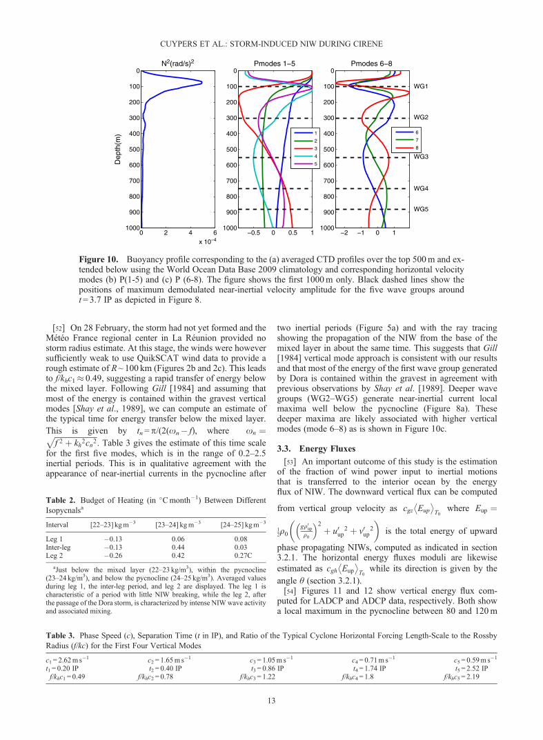
estimate of the contribution of NIW to the diffusive heat fluxis striking: the depth-averaged heat flux is reduced by a fac-tor of 10 when the near-inertial signal is not considered(Figure 15b).[64] A more detailed view is provided in Figure 16a with a

time-depth plot of the diffusive heat flux. Q has typical neg-ative values of 10–50Wm�2, corresponding to a downwarddiffusive transport of heat, with increased values during thecyclone and post-cyclone periods. Downward turbulent fluxis first strong just beneath the mixed layer at the end of thepre-cyclone and during the cyclone period and then extendsdownward. Depths of maximum downward heat transportfollow a similar pattern to that of increased shear along theNIW path (Figure 14a) and also match the depth of maxi-mum shear for baroclinic modes 4 and 5, illustrating againthe important role of NIW.[65] Another way to estimate the impact of turbulent diffu-

sion is to compute the local heating rate @ z(Kd @ zT)(Figure 16b). Depths of increased local heating and coolingappear along the trajectory of the internal gravity wavepacket excited locally at the mooring during the storm.Fairly large values are observed, with up to 10 �Cmonth�1

Figure 14. (a) Vertical shear of the velocity modulus (computed at 4m vertical resolution). The blacklines show NIW rays trajectories computed from the vertical group velocity (see text for details). Thewhite lines represent the vertical structure of the shear associated with the first five baroclinic modes(dPn/dz). (b) Inverse of the Richardson number. The white dashed line indicates the mixed layer depth.


18

locally and a dominance of heating over cooling after theonset of the storm (note that, in comparison, the effect ofpenetrative solar heat flux is about ~0.5 �Cmonth�1 at40m and decreases exponentially below). We also averagedthe heating rate between different isopycnals in order to pro-vide a more quantitative assessment of the role of mixing(Figure 16 and Table 2). Three intervals have been chosenthat correspond respectively to the layer just below themixed layer (22–23 kgm�3, layer L1), within the thermo-cline/pycnocline (23–24 kgm�3, layer L2), and below thethermocline/pycnocline (24–25 kgm�3, layer L3). The tem-poral evolution for each isopycnal-averaged heating rate isdisplayed in Figure 16c. The general opposition betweenthe heating rate for L1 (mostly cooling) and L2/L3 (mostlyheating) illustrates clearly the downward transport ofheat by mixing (heat is removed from below the mixedlayer to warm deeper levels). Except for a mixing event dur-ing the pre-cyclone period, the frequency of surface cooling/

subsurface heating events increases as time goes on, withmost events occurring during the post-cyclone period.Heating events also occur later within L3 than within L2,which is consistent with NIW downward propagation. Theaverage heating rate for L3 increases from 0.03 �Cmonth�1

during the cyclone period and up to 0.27 �Cmonth�1 duringthe post-cyclone period. In contrast, the average heating rateof about 0.4 �Cmonth�1 within L2 is almost unchangedduring the cyclone and post-cyclone periods. The averagevalues in Table 2 also allows for quantification of theincrease in heating by vertical mixing associated withNIW. During the pre-cyclone period (characterized by littleor no NIW activity), the average heating rate due to mixingis ~0.06 �Cmonth�1 in the thermocline and 0.08 �Cmonth�1 below. During the post-cyclone period character-ized by strong NIW in the thermocline and below, thoseheating rates increase to 0.42 �Cmonth�1 and 0.27 �Cmonth�1, respectively.

Figure 15. Estimates of dissipation rate and eddy diffusivity at the ATLAS mooring inferred from shearusing mooring data: (a) dissipation rates e averaged over leg 1 (in blue), inter-leg (in black) period, and leg2 (in red); (b) same as Figure 15a but for eddy diffusivity, Kd; and (c) mean profile of e averaged over theentire period: e inferred from total shear is displayed in dark blue, whereas e inferred from total shearminus inertial shear in black. Vertical heat flux at the ATLAS mooring: (d) profile of vertical diffusive heatflux time averaged over leg 1 (blue), inter-leg period (black), and leg 2 (red); (e) profile of vertical diffusiveheat flux time averaged over leg 2 with (blue) and without (black) the contribution of near-inertial currents tothe vertical turbulent diffusivity.


19

5. Summary and Discussion

5.1. Summary

[66] The Cirene cruise provides a 1month long record ofair-sea interface and subsurface high frequency observationsin the southwestern tropical ocean in early 2007. During thecruise, a tropical storm formed almost exactly at the locationof a ship station and ATLAS mooring deployed during thecruise (8�S, 67�E) and later developed into tropical cycloneDora. This provides an opportunity to describe the upperocean response to strong atmospheric forcing and generationof NIW at this climatically relevant site of the Indian Ocean[Xie et al., 2002; Vialard et al., 2009]. Weak winds (<5ms�1), shallow mixed layers (~20m) and intense downwardsolar radiation characteristic of a break phase of the Madden-

Julian oscillation preceded the cruise. This was followed by aperiod of strong winds (~10ms�1 and wind stresses of ~0.2Nm�2, i.e., characteristic values for a tropical depression) and~300mm of cumulated rainfall as the storm formed andtraveled southward over the cruise site (25 January to 2February 2007). Weaker winds then progressively returned asDora intensified but moved away. The oceanic response wascharacterized by a ~2�C cooling of the sea surface and asuppressed the diurnal cycle.[67] In response to the storm, a clear NIW response was

seen in the velocity field within the oceanic mixed layerfor about 1week after the passage of the storm. Inertialpumping in the mixed layer drove NIW that propagatedvertically into the interior ocean, as illustrated by clearupward phase propagation in the velocity field. Phase

Figure 16. (a) Time depth plot of vertical diffusive heat flux at the ATLAS mooring; (b) same asFigure 16a for the heating rate; for each plot, black lines represent isopycnal contours [22–25] kgm�3;thick black plain and dashed lines represent near-inertial waves ray characteristics for WG1m and magentadashed line represents the mixed layer depth. (c) Temporal evolution of the heating rate at M averagedbetween isopycnals [22,23], [23,24], and [24,25] kgm�3.


20

analysis of the upward-propagating part of the velocity fieldidentifies five wave packets in the data. The first wave group(WG1) had current variations of ~0.25m s�1 within andbelow the pycnocline (100–200m). The deepest wavepacket had an amplitude of ~0.15m s�1and propagatesbelow 1000m, the maximum depth of the measurements.[68] We then identified the main characteristics of each

wave packet (e.g., horizontal and vertical wave numbers,and intrinsic frequency), largely based on the methodproposed by Alford and Gregg [2001]. The first two wavegroups (identified in the upper 400m) had rather largehorizontal scales (~200–300 km), comparable to horizontalscales in the forcing before the eye formation, and appearedto propagate northward. The deeper-identified wave groups(500–1000m) appeared to have smaller horizontal scales(~80 km), and some of them displayed apparent southwardpropagation. All wave packets carried energy downward:~2mWm�2 down to 400m for WG1 and WG2 and ~1mWm�2 down to 1000m for WG3–WG5. While it is difficult tocompare this vertical energy flux to the wind power inputfrom measurements at a single location, it is interesting tonote that the maximum vertical energy flux at thermoclinelevel (between 60 and 120m) corresponds to about 10% ofthe maximum surface wind power input, implying that anon-negligible fraction of the energy input of thisdeveloping storm penetrated below the thermocline.[69] Finally, we diagnosed the potential influence of those

NIW on mixing in the interior ocean (i.e., below the mixedlayer). There was twofold increase of the kinetic energy dis-sipation rate in the interior ocean between the pre-cycloneperiod (with little internal wave propagation in the interiorocean) and post-cyclone period. A simple vertical mixingparameterization identified a downward vertical mixing heatflux within the thermocline of ~10Wm�2 during the pre-cy-clone period versus approximately �25Wm�2 during thecyclone period and �35Wm�2 during the post-cycloneperiod (which was also the main period of internal waveactivity). The associated heat flux convergence resulted inaverage mixing-induced heating rates within the thermoclineof ~0.42 �Cmonth�1 during the post-cyclone period versusonly 0.06 �Cmonth�1during the pre-cyclone period. Thissuggests a strong increase of vertical mixing in thethermocline associated with the increase of vertical shearalong the paths of downward-propagating internal waveenergy.

5.2. Discussion

[70] The vertical NIW energy flux (~2.5mWm�2) in-duced by Dora is comparable to other estimates of baroclinicNIW energy fluxes generated by moderate to strong windevents. Qi et al. [1995] estimated 2–6mWm�2 of downwardNIW energy fluxes as the result of storms in the NortheastPacific (47�N) Ocean. At a latitude of 6.5�S comparable toCirene (8�S), Alford and Gregg [2001] estimated NIW bar-oclinic downward energy flux of 2mWm�2 as the result ofstrong monsoon winds in the Banda Sea. However, energyfluxes associated with a fully developed hurricane can bemuch larger. For instance Jaimes and Shay [2010] found adownward NIW energy flux of 79mWm�2 and an upwardenergy flux of 254mWm�2 associated with HurricaneKatrina. In their case, energy fluxes corresponded to acategory 5, fast moving hurricane and were estimated for

conditions inside geostrophic vortices that often are foundto enhance vertical near-inertial wave propagation. Althoughthey did not estimate vertical energy fluxes, Sanford et al.[2007] found near-inertial horizontal velocities reaching�1.5m s�1 just after the passage of Hurricane Frances.[71] In this paper, we distinguish three different NIW

groups (WG3–WG5) at depth (z> 500m) at the mooring lo-cation. These wave groups show significant near-inertialcurrent amplitude (up to 30 cm s�1) and vertical energyfluxes of up to 1mWm�2 (Figures 8 and 11), which suggestthat their energy efficiently propagated downward from thesurface. They were however not related to Dora or any othertropical storm or cyclone in the region. They are moreovercharacterized by relatively short horizontal wavelengths.This may be due to the very fine scale of the backgroundatmospheric forcing in this region, where mesoscaleconvective variability can induce wind variations on spatialscales of a few kilometers to a few tens of kilometers. In addi-tion, WG3 propagates poleward whereas equatorward propaga-tion is expected from the b effect dispersion [Garrett, 2001].The background vorticity field may however have influencedthe propagation of these wave groups. Background vorticityz indeed shifts the inertial frequency to an effective inertialfrequency feff= f+1/2z. Such modification of feff can be muchlarger than the variation of f on the b plane and explainpoleward propagation. At midlatitudes, where eddy variabilityis often strong, observations show a strong impact of mesoscalevorticity on NIW propagation [Kunze, 1995; Jaimes and Shay,2010]. Mesoscale activity at the low latitude Cirene location(8�S) is however much weaker, but the deep, westward jet gen-erated by the Indian Ocean Dipole [Vialard et al., 2009] mayhave produced such modifications of the background vorticity.Figure 17 shows a very rough proxy of this vorticity from the

meridional shear � @u@y

� �of the surface zonal velocity u

recorded by the ship ADCP along a meridional transect at67�E between 1 and 14 January and smoothed using a runningmean of 40km. The order of magnitude of feff variations at thesurface obtained from this estimate (Figure 17) is larger thanthe equatorward inertial frequency decrease from the b effect

−9 −8.5 −8 −7.5 −70.9

0.95

1

1.05

1.1

1.15

Latitude(°S)

f eff/f

3

3.5

4

4.5

5

5.5

x 10−10

f2

Figure 17. Ratio of surface effective inertial frequency feffand inertial frequency f along a 67�E transect, estimatedfrom the ship ADCP zonal velocity shear in black line.Red line is squared surface effective inertial frequency feff

2

and red dashed line is f2.


21

at the ATLAS mooring and FP station (red curve). Near 8�S,feff has a local maximum, which may allow southwardpropagation in addition to the more classical equatorwardpropagation. Note that the wave will conserve its intrinsicfrequency while propagating at depth and will be able topropagate poleward until its intrinsic frequency equals the localeffective frequency. Clearly the effective frequency at thesurface and at depth can be different, and an accuratecomputation of the generation point and turning point locationfor each wave group would require knowledge of the 3-Dmesoscale field. We leave a quantitative computation of raypath in space and time for future modeling studies.[72] This paper suggests that a non-negligible part (~10%)

of the energy injected into inertial currents by the storm maypropagate below the mixed layer under the form of NIW.This energy escapes the mixed layer to be dissipated withinthe pycnocline and in the deep ocean. The passage of theNIW triggered by Dora for example induces significant mix-ing and heating rates in the pycnocline. Generation of NIWhence appears as an efficient mechanism to redistributemomentum and induce mixing below the mixed layer. Asa consequence, fast propagation of NIW at depth can reducestorm-induced mixing in the surface layer and hence the sur-face cooling, as shown by Jaimes and Shay [2010] afterHurricanes Katrina and Rita. We can therefore expect a cli-matic impact of NIWs, notably in regions of strong ocean at-mosphere interactions as the Cirene region [e.g., Xie et al.,2002; Vialard et al., 2009]. The very local nature of themeasurements collected during the cruise does not allow usto investigate in detail the influence of the associated mixingon the ocean thermal structure, nor the fate of the energy thatis injected in the deep ocean. Furthermore, while Cirenemeasurements are interesting because of the intense air-seacoupling in this region, the location where maximum cy-clone intensity (and energy transfer to the ocean) occurredwas further south.[73] A good representation of NIW generation,

propagation, and dissipation is needed in Ocean GeneralCirculation Models (OGCMs) in order to characterize theclimatic impact of NIW energy. Although horizontalresolution of state-of-the-art OGCMs is generally sufficientto represent cyclones and storms-induced NIWs, two diffi-culties arise. First, atmospheric forcing at very fine scale(e.g., the very strong winds within the cyclone eyewall) isnot resolved by current re-analysis products, which are usedto force the OGCMs (horizontal resolution of 10 km isprobably necessary to resolve the basic eye and eyewallstructure in the atmospheric forcing, Halliwell et al.,2011). Second, the use of current parameterizations of dissi-pation such as the turbulent kinetic energy (TKE)-based pa-rameterization [Mellor and Yamada, 1982] and the use ofgeopotential coordinates [Levaillant, 2009] result in an arti-ficial damping of internal waves. Leclair and Madec [2011]recently proposed new vertical coordinates that reduce theartificial damping on NIWs and may result in a better repre-sentation of internal waves in high resolution OGCMs. Amore physically relevant parameterization of internalwave-induced dissipation may then be implemented fromthe most recent formulations [Gregg, 1989; Kunze, 2006].Vincent et al. [2011a, 2011b] have developed an interestingframework to include tropical cyclone wind forcing in a

general circulation model. We aim at using this frameworkin a relatively high resolution (1/4�) model of the IndianOcean, in order to study the effect of NIW at large spatialscales and seasonal time scales.[74] Finally, we also observed clear energy peaks at the

diurnal and semidiurnal time scale, associated to internaltides. Internal tides are indeed expected in this region,where a mid-ocean ridge (see Figure 1b) is associated withrugged bottom topography. The stronger mixing in thepycnocline observed during post-cyclone period is clearlyassociated with NIW, but as opposed to the sporadic forc-ing of NIW by tropical depressions or cyclones, tidal forc-ing is ever present and internal tidal mixing is probablyimportant for the longer term heat budget. We will discussand pursue this topic in a separate paper on the basis ofthese observations and a simple linear internal tide model(Cuypers et al., manuscript in preparation, 2013).

[75] Acknowledgments. We thank Claudie Marec from INSU andJacques Grelet from IRD for their technical support in the deployment ofthe mooring, collection of the CTD/LADCP profiles, and the processingof the data. B. Luong implemented the Schütze and Schwetlick free-knotspline algorithm that we use to isolate wave groups. JV is funded by Institutde Recherche pour le Développement (IRD). MJM is funded by NOAA.The LEFE/IDAO program of the CNRS (Centre National de la RechercheScientifique) also supported this work. This is PMEL Contribution 3804.

ReferencesAlford, M. H. (2001), Internal swell generation: The spatial distribution ofenergy flux from the wind to mixed layer near-inertial motions, J. Phys.Oceanogr., 31, 2359–2368.

Alford, M. H., (2003), Improved global maps and 54-year history of wind-work on ocean inertial motions, Geophys. Res. Lett., 30, 1424.doi:10.1029/2003GL018543.

Alford, M. H., and M. C. Gregg (2001), Near-inertial mixing: Modulation ofshear, strain and microstructure at low latitude, J. Geophys. Res., 106, C8,16,947–16,968.

Bentamy, A., K. B. Katsaros, M. Alberto, W. M. Drennan, and E. B. Forde(2002), Daily surface wind fields produced by merged satellite data.Amer. Geophys. Union, Geophys. Monogr. Ser., 127, 343–349.

Bonjean, F., and G. S. E. Lagerloef (2002), Diagnostic model and analysisof the surface currents in the tropical Pacific Ocean. J. Phys. Oceanogr.,32, 2938–2954.

Bouruet-Aubertot, P., H. Mercier, F. Gaillard, and P. Lherminier (2005),Evidence of strong inertia gravity wave activity during the POMMEexperiment. J. Geophys. Res., 110, doi:10.1029/2004JC002747, 2005.

Broecker, W. S. (1991), The great ocean conveyor. Oceanography, 4, 79–89.Cairns, J. L. and G. Williams (1976), Internal waves observation from a midwater float, J. Geophys. Res., 81: 1943–1950.

Chang, S. and R. Anthes (1978), Numerical simulations of the ocean’snonlinear baroclinic response to translating hurricanes. J. Phys.Oceanogr., 8, 468–480.

Fairall, C. W., E. F. Bradley, J. E. Hare, A. A. Grachev, and J. B. Edson,(2003), Bulk parameterization of air-sea fluxes: Updates and verificationfor the COARE algorithm. J. Climate, 16, 571–591.

Fofonoff, N. P., (1969), Spectral characteristics of internal waves in theocean, Deep Sea Res., 16, (Suppl.), 59–71.

Foltz, G. R., J. Vialard, B. Praveen Kumar and M. J. McPhaden (2010),Seasonal mixed layer heat balance of the southwestern tropical IndianOcean, J. Clim., 23, 947–965.

Furuichi, N., T. Hibiya, and Niwa Y. (2008), Model-predicted distributionof wind-induced internal wave energy in the world’s oceans. J. Geophys.Res. 113, C09034. doi:10.1029/2008JC004768.

Garrett, C. (2001), What is the “near-inertial” band and why is it differentfrom the rest of the internal wave spectrum? J. Phys. Oceanogr., 31,962–971.

Geisler, J. E. (1970), Linear theory on the response of a two layer ocean to amoving hurricane. Geophys. Fluid Dyn., 1, 249–272.

Gerkema T. and J. T. F Zimmerman (2008), Lecture notes Royal NIOZ,Texel.

Gill, A. E. (1982), Atmosphere-Ocean Dynamics, Academic Press, 662 pp.Gill, A. E. (1984), On the behavior of internal waves in the wake of storms.J. Phys. Oceanogr., 14, 1129–1151.


22

Gregg, M. C., (1989), Scaling turbulent dissipation in the thermocline. J.Geophys. Res., 94, 9686–9698.

Halliwell, G., Shay L. K., J. K. Brewster, and W. J. Teague (2011),Evaluation and sensitivity analysis to an ocean model to Hurricane Ivan.Mon. Wea. Rev., 139, 921–945.

Hebert, D., and J. N. Moum (1994), Decay of near inertial wave. J. Phys.Oceanogr., 24, 2334–2351.

Jaimes, B. and L. K. Shay (2009), Mixed layer cooling in mesoscaleoceanic eddies during Hurricanes Katrina and Rita. Mon. Wea. Rev.,137, 4188–4207.

Jaimes, B. and L. K. Shay (2010), Near-inertial wave wake of HurricanesKatrina and Rita over mesoscale oceanic eddies. J. Phys. Oceanogr.,40, 1320–1337.

Jaimes, B., Shay L. K., and G. R. Halliwell (2011), The response of quasigeostrophic oceanic vortices to tropical cyclone forcing. J. Phys.Oceanogr., 41, 1965–1985.

Jayakumar, A., J. Vialard, M. Lengaigne, C. Gnanseelan, J. P. McCrearyand B. Praveen Kumar (2011), Processes controlling the surface temper-ature signature of the Madden-Julian oscillation in the thermocline ridgeof the Indian Ocean, Clim. Dyn., 37, 2217–2234.

Knapp, K. R., M. C. Kruk, D. H. Levinson, H. J. Diamond, and C. J. Neu-mann (2010), The International Best Track Archive for Climate Steward-ship (IBTrACS). Bull. Amer. Meteor. Soc. 91, 363–376.

Koch-Larrouy A., M. Lengaigne, S. Masson, G. Madec, P. Terray (2008),Tidal mixing in the Indonesian Seas and its effect on the tropical climatesystem. Clim. Dyn. 34(6): 891–904, doi:10.1007/s00382-009-0642-4.

Kunze, E., (1985), Near-inertial wave propagation in geostrophic shear. J.Phys. Oceanogr., 15, 544–565.

Kunze, E., (1995), The energy balance in a warm-core ring’s near-inertialcritical layer. J. Phys. Oceanogr., 25, 942–957.

Kunze, E., E. Firing, J. M. Hummon, T. K. Chereskin, and A. M. Thurnherr(2006), Global abyssal mixing inferred from lowered ADCP shear andCTD strain profiles. J. Phys. Oceanogr., 36, 1553–1576.

Leaman, K. D. (1976), Observations of vertical polarization and energy fluxof near-inertial waves. J. Phys. Oceanogr., 6, 894–908.

Leclair, M., and G. Madec (2011), eZ-coordinate, an arbitrary Lagrangian–Eulerian coordinate separating high and low frequency motions. OceanModelling 37(3-4): 139–152.

Levaillant, X. (2009), Ondes internes générées par le forçage atmosphériquedans l’océan Indien subtropical: modélisation et mesures in situ. ThesisUniversité Paris 6.

Lloyd, I. D. and G. A. Vecchi (2010), Submonthly Indian ocean coolingevents and their interaction with large-scale conditions. J. Climate, 23,700–716.

Locarnini, R. A., A. V. Mishonov, J. I. Antonov, T. P. Boyer, H. E. Garcia,O. K. Baranova, M. M. Zweng, and D. R. Johnson (2010), World OceanAtlas 2009, Volume 1: Temperature, edited by S. Levitus, pp. 184,NOAA ATLAS NESDIS 68, U.S. Government Printing Office,Washington, D.C.

MacKinnon, J. A. and M. C. Gregg (2005), Spring mixing: Turbulence andinternal waves during restratification on the New England Shelf. J.Geophys. Res., 35, 2425–2443.

Marotzke, J., and J. R. Scott (1999), Convective mixing and thethermohaline circulation. J. Phys. Oceanogr., 29, 2962–2970.

Mellor, G. L. and T. Yamada (1982), Development of a turbulence closuremodel for geophysical fluid problems. Rev. Geophys., 20, 851–875.

McCreary, J. P., P. K. Kundu and R. L. Molinari (1993), A numericalinvestigation of dynamics, thermodynamics and mixed-layer processesin the Indian Ocean, Prog. Oceanogr., 31, 181–244.

McPhaden, M. J., G. Meyers, K. Ando, Y. Masumoto, V. S. N. Murty, M.Ravichandran, F. Syamsudin, J. Vialard, L. Yu, and W. Yu (2009),RAMA: The research moored array for African-Asian-Australian mon-soon analysis and prediction. Bull. Am. Meteorol. Soc., 90, 459–480.

Munk, W., and Wunsch, C. (1998), Abyssal recipes II: Energetics of tidaland wind mixing. Deep-Sea Res. I, 45, 1977–2010.

O’Brien, J. J., and R. O. Reid (1967), The non-linear response of a two-layer,baroclinic ocean to a stationary, axially-symmetric hurricane: Part I.Upwelling induced by momentum transfer. J. Atmos. Sci., 24, 197–207.

Osborn, T. R. (1980), Estimates of the local rate of vertical diffusion fromdissipation measurements. J. Phys. Oceanogr., 10, 83–89.

Park, T. W, and C. S. Burrus (1987), Digital filter design. John Wiley &sons.

Perkins, H. (1970), Inertial oscillations in the Mediterranean, Ph D. thesis.Massachusetts Institute of Technology, Woods Hole, 155 pp.

Pollard, R. T. (1970), On the generation by winds of inertial waves in theocean. Deep Sea Res., 17, 795–812.

Price, J. F. (1981), Upper ocean response to a hurricane. J. Phys. Oceanogr.,11, 153–175.

Qi, H., R. A. De Szoeke, C. A. Paulson, and C. C. Eriksen (1995), Thestructure of near-inertial waves during ocean storms. J. Phys. Oceanogr.,25, 2853–2871.

Saji, N. H., B. N. Goswami, P. N. Vinayachandran and T. Yamagata (1999),A dipole mode in the tropical Indian Ocean. Nature, 401, 360–363.

Sanford, T. B., Price J. F., Girton, J. B. and Webb D. C. (2007), Highlyresolved observations and simulations of the ocean response to ahurricane. Geophys. Res. Lett. 34, L13604.

Schott, F. A., S.-P. Xie, and J. P. McCreary Jr. (2009), Indian Oceancirculation and climate variability, Rev. Geophys., 47, doi:10.1029/2007RG000245.

Shay, L. K., R. L. Elsberry, and P. G. Black (1989), Vertical structure of theocean current response to a hurricane. J. Phys. Oceanogr., 19, 1249–1269.

Shütze, T. and Schwetlick (1997), Constrained approximations by splineswith freeknots. BIT, 37:1, 105–137.

Smith, W. H. F. and D. Sandwell (1997), Global sea floor topography fromsatellite altimetry and ship depth soundings. Science, 26, 277(5334):1956–1962.

Sriver, R. L. and M. Huber (2007), Observational evidence for an oceanheat pump induced by tropical cyclones, Nature, 447, 577–580.

Torrence, C. and G. P. Compo (1998), A practical guide to wavelet analysis,Bull. Am. Meteorol. Soc., 79, 61–78.

Vialard, J., G. Foltz, M. J. McPhaden, J. P. Duvel and C. de Boyer Montégut(2008), Strong Indian Ocean sea surface temperature signals associatedwith the Madden-Julian oscillation in late 2007 and early 2008.Geophys. Res. Lett., 35, L19608, doi:10.1029/2008GL035238.

Vialard, J., et al., (2009), Cirene: Air-sea interactions in the seychelles-chagosthermocline ridge region. Bull. Am. Meteor. Soc. 90(1), 45–61.

Vinayachandran, P. N., J. Kurian, and C. P. Neema, (2007), Indian Oceanresponse to anomalous conditions in 2006. Geophys. Res. Lett., 34,L15602, doi:10.1029/2007GL030194.

Vincent, E., M. M. Lengaigne, G. Madec, J. Vialard, G. Samson,N. Jourdain, C. E. Menkes and S. Jullien (2012a), Processes setting thecharacteristics of sea surface cooling induced by tropical cyclones, J.Geophys. Res., 117, C02020, doi:10.1029/2011JC007396.

Vincent, E., M. M. Lengaigne, J. Vialard, G. Madec, N. Jourdain, andS. Masson (2012b), Assessing the oceanic control on the amplitude ofsea surface cooling induced by tropical cyclones, J. Geophys. Res., 117,doi:10.1029/2011JC007705.

Von Storch J. S., H. Sasaki, and J. Marotzke (2007), Wind-generated powerinput to the deep ocean: an estimate using a 1/10� general circulationmodel. J. Phys. Oceanogr. 37, 657–672.

Watanabe, M. and T. Hibiya (2002), Global estimates of the wind-inducedenergy flux to inertial motions in the surface mixed layer, J. Geophys.Res., 29, 1239–1247.

Webster, P. J., A. M. Moore, J. P. Loschnigg, and R. R. Leben (1999), Cou-pled oceanic atmospheric dynamics in the Indian Ocean during 1997–98,Nature, 401, 356–360.

Wunsch, C. (1998), The work done by the wind on the ocean generalcirculation model. J. Phys. Oceanogr., 28, 2332–2340.

Wunsch, C., and R. Ferrari (2004), Vertical mixing, energy and the generalcirculation of the oceans. Ann. Rev. Fluid Mech., 36, 281–314.

Xie, S.-P., H. Annamalai, F. A. Schott and J. P. McCreary (2002), Structureand mechanisms of south Indian climate variability, J. Climate, 9, 840–858.

Zhai, X., Greatbatch, R. J. and E. Carsten (2007), Spreading of near-inertialenergy in a 1/12� model of the North Atlantic Ocean. Geophys. Res. Lett.,34, L10609, doi:10.1029/2007GL029895.

Zhai, X., Greatbatch, R. J. and E. Carsten (2009), On the loss of wind-inducednear-inertial energy to turbulent mixing in the upper ocean. J. Phys.Oceanogr., 39, 3040–3045.

Zhang, C., (2005), Madden-Julian Oscillation, Rev. Geophys., 43, RG2003,doi:10.1029/2004RG000158.


23

Tropical storm-induced near-inertial internal waves during the Cirene experiment: Energy fluxes and...

Documents

Transcript of Tropical storm-induced near-inertial internal waves during the Cirene experiment: Energy fluxes and...