Deep-Sea Research 1, Vol 40, No 7, pp 1345-1358, 1993 09674)637/93 $6 00 + 0 t'10 Printed m Great Britain © 1993 Pergamon Press Ltd

Mixing in the Brazil-Malvinas Confluence

ALEJANDRO A. BIANCHI,* CLAUDIA F. GIULM*t and ALBERTO R. PIOLA*

(Received 24 April 1992, m revised form 13 October 1992; accepted 21 October 1992)

Abstract--Conductwity-temperature-depth profile data from the Western Argentine Basin collected from 1984 to 1989 are used to quantify the cross-front heat and salt transfers associated with the vertical finestructure across the Brazil-Malvmas Confluence The fluxes are estimated following the statistical model of JoYcE (Journal of Physical Oceanography, 7,626-629, 1977). The data indicate that the upper ocean cross-front structure of the large-scale temperature and sahnlty fields is constant

The medium-scale finestructure mtenslty is quantified by the variance of the vertical temperature and sahmty gra&ents m the 10-100 m wavelength band Due to the abundance of intrusions, the upper layer (0--1000 m) variances increase by a factor of four at &stances <20 km from the front Heat and salt flux estimates associated with medium-scale mixing in the upper ocean are of the order 10-2°C m s -I and 10 -3 m s -1 respectively. These fluxes are an order of magnitude greater than available estimates for other frontal regions. The medium-scale finestructure may therefore play a key role in the &ssipatlon of eddies and intrusive lenses in the region. Heat and salt fluxes between North Atlantic Deep Water and Circumpolar Deep Water are 6.5 x 10 -4 °C m s -1 and 1.8 × 10 -4 m s -i , and agree w~th ex~stmg estimates

Extrapolation of upper layer Brazil-Malwnas Confluence cross-frontal fluxes to the Subtropical Convergence across the South Atlantic suggests that the medmm-scale southward heat flux is about 20% of the oceamc northward heat flux at 30°S Similarly, the freshwater flux balances 20% of the excess evaporation north of 30°S.

INTRODUCTION

THE At lan t ic is character ized by two sources of deep water masses in the n o r t h e r n and

sou thern regions, and therefore is the bas in in which mos t active renewal of abyssal waters of the Wor ld Ocean occurs. W i t h i n the South At lan t i c , the A r g e n t i n e Bas in is un ique because of its locat ion at the crossroads of several ma jo r water masses (CONFLUENCE PRINCIPAL INVESTIGATORS, 1990). C o n s e q u e n t l y , several ex t r ema are found in vertical p roper ty dis t r ibut ions . REID et al. (1977) have ident i f ied seven dist inct water masses below the the rmoc l ine in the W e s t e r n South At lan t ic . The subt ropica l uppe r water , usually referred to as South At lan t i c Cen t r a l W a t e r ( S A C W , fol lowing SVERDRUP et al., 1946) is advected in to the region by the Brazil Cu r r en t . S A C W is character ized by t empera tu res higher than 10°C (up to 23°C in the surface layer) and sal ini t ies h igher than 35 P S U (up to 36 PSU) . The Subanta rc t i c W a t e r ( S A A W , also re fe r red to as Malv inas W a t e r ; GOROON, 1981) advected no r thward in the uppe r 500 m of the Malv inas Cu r r e n t has t empera tu res

*Departamento Oceanograffa, SerVlClO de Hldrograffa Naval, Av Montes de Oca 2124, 1271 Buenos Aires, Argentina

tAlso at Conselo Nacional de Investigaoones Cmntificas y T6cmcas de la Repdbhca Argentina

1345

1346 A A. BIANCHI et al

I I I ! I I I I I

o._.~

g~./ ~/cowl

~ 3 3 7 5 3 4 2 5 $ 4 7 5 ~ 2 5 5 5 7 5 3 6 2 5

Sohn#y FIg 1 Potential temperature sahn]ty diagrams for Stas 2-4 of cruise OACF89 The statmn

positions are shown in Fig 2

lower than 10°C and salinities lower than 34.3 PSU. At intermediate depth, a minimum salinity layer (WOST, 1935) characterizes the Antarctic Intermediate Water (AAIW). The core of AAIW in this region is found at a depth range of 800 to 1000 m. Salinity values close to 34.2 PSU, potential temperatures from 3.7 to 4.8°C and a density (ao) interval from 27.05 to 27.20 (PIOLA and GORDON, 1989) characterize this water mass.

Below the intermediate water and within the 36.75-37.15 o2 density range (REID et al., 1977), Circumpolar Deep Water (CDW) co-exists with North Atlantic Deep Water (NADW). These water masses are located within the depth range of 1000-3200 m. Excluding the uppermost layers, the core of NADW represents the maximum in the vertical salinity distribution (DEACON, 1933, 1937; WOST, 1935).

The upper water general circulation of the Western Argentine Basin is characterized by the southward flow of the Brazil Current along the continental margin of South America and the equatorward flow of the Malvinas Current along the continental slope. The encounter of both currents near 38°S causes a strong thermohaline front referred to as Brazil-Malvinas Confluence (GORDON, 1989; RODEN, 1986). This region stands out by the high mesoscale variability observed in high-resolution infrared imagery (LErECgIS and GORDON, 1982; OLSON et al., 1988), satellite-tracked drifting buoys (PATTERSON, 1985; PIOLA et al., 1987) and satellite altimetry (CHENEY et al., 1983; ZLOTNICra and Fu, 1989).

Associated with the Brazil-Malvinas Confluence, the variety of water masses and the large eddy variability, a complex vertical thermohaline structure is found. O-S distribution at three consecutive CTD stations show (Fig. 1) a typical subantarctic structure (Sta. 2), while two stations away (Sta. 4) the structure is subtropical. The most remarkable differences in O-S space occur at densities lower than o0 = 27.25, e.g. at the thermocline and at the core of the AAIW (PIOLA and GEORGI, 1982). Station 3, located at the front, shows layering of the different water masses characteristic of the Confluence region. These

Mixing m the Brazll-Malvlnas Confluence 1347

structures act to enhance the transfer of heat and salt by a variety of physical processes such as double-diffusion, dyapycnal mixing and cross-front lateral mixing.

The variability observed in the vertical thermohaline structure is believed to be associated with heat and salt transfer across the Brazil-Malvinas Confluence (GEoRGI, 1981; PIOLA and GEORCI, 1982). A joint Argentine-French-U.S. program, known as Confluence, was carried out in the Brazil-Malvinas Confluence to study the local dynamics of the front, and its time and space variability. One objective of the program was to quantify the small- and medium-scale mixing across the frontal regions (CONFLUENCE PRINCIPAL INVESTIGATORS, 1990). In this paper we evaluate the amount of heat and freshwater transferred across the Brazil-Malvinas Confluence by small-scale mixing processes, following the statistical model proposed by JOYCE (1977). In this model, the small-scale diffusion of heat and salt across intrusions is balanced by horizontal advection due to lateral mixing. Estimates of heat and salt fluxes are made in two different density ranges: (1) between SACW and SAAW/AAIW and (2) between CDW and NADW.

The results are compared with existing flux estimates in other regions of the world ocean. Finally, the potential impact of the cross-front property transfer in the Atlantic large-scale meridional heat and freshwater balances is investigated.

DATA AND METHODS

The work presented here is based on the analysis of conductivity-temperature-depth (CTD) observations from the Brazil-Malvinas Confluence taken during five cruises from November 1984 through September 1989 (Table 1; Fig. 2). Also shown in Fig. 2 is the density distribution (oo) at 500 m depth computed from historical data (PIOLA and GARCIA, in press) showing the climatological flow patterns at mid-thermocline depth.

The temperature and salinity finestructure have been quantified in two different depth ranges, one between the base of the mixed layer and the core of the AAIW and the other between the 36.75 and 37.05 or E range. These ranges were selected in order to estimate the salt and heat lateral fluxes between the SACW-SAAW/AAIW and NADW-CDW, respectively.

Following STERN (1967) the property (cI)) is decomposed as follows:

¢ = U p + ~ + ¢ ' , (1)

where Up is the mean property field corresponding to the large-scale property structure of the water masses with typical horizontal scales of more than 100 km and vertical scales of 1000 m; 4a is the medium-scale departure from the mean field with small aspect ratio and small vertical velocity; and ¢ ' is the small-scale property field due primarily to instabilities

Table 1. Conducttvtty--temperature--depth data used m th~s study

Cruise Shtp Date Reference

PD0284 Puerto Deseado Nov 1984 GUERRERO et al. (1986) OA0485 Capttdn Oca Balda Jun. 1985 GU~RRERO et al (1986) PD0288 Puerto Deseado Apr. 1988 CHARO el al. (1991) PDCF88 Puerto Deseado Nov. 1988 CHARO et al (1991) OACF89 Capudn Oca Balda Sep 1989 CI-~Ro et al. (1991)

1348 A A BIANCHI et al

60 ° 50 ° 400

60* 50* 40*

F~g. 2 Posmon of the CTD stat ions used to es t imate the intensity of the tempera ture and salinity flnestructure. Also shown is the climatological densi ty o0 d~stnbution at 500 m (from PIOLA and GARCiA, in press) Open circles indicate sections crossing the front. Sta tmns 2-4 of Fig. 1 are shown.

of the medium-scale and which effectively causes the vertical exchange across the medium-scale interfaces.

Based on the temperature and salinity conservation equations for the medium-scale field, JOYCE (1977) has shown that in order to achieve steady-state balance the following must be satisfied:

a,,i, + = ox-2 ,3 0, (2)

where u, are the velocity components in the x, directions (i = 1,2, 3), ~i~, is the vertical eddy diffusivity and 6,3 = 0 for i = 1, 2 and ~33 = 1. Neglecting vertical velocities in the low aspect ratio medium-scale property field with the x coordinate oriented along the front, equation (2) reduces to:

f0,]2/0 ~ = - A e L-~z j / ~ - y (3)

where y is the direction normal to the front. Practical difficulties arise associated with the medium-scale property fluxes calculated from equation (3). First, estimates of the vertical eddy diffusivity vary by two orders of magnitude (GARRET, 1979). VOORmS et al. (1976) have estimated a vertical diffusivity of 5 x 10 - 4 m 2 s - 1 in the vicinity of water mass boundaries. A value of A = 10 -4 m 2 s -1 which is an harmonic mean between low central gyre values and high values (JOYCE et al . , 1978), is used in this study. This value has been used in previous studies (JOYCE, 1977; JOYCE et al. , 1978; GEORG], 1981; PIOLA and GEORG], 1982) based on this model. This procedure allows us to compare our results on the basis of the property variances and horizontal gradients.

Mixing m the Brazll-Malvmas Confluence 1349

Vertical temp gradient (°C/dbor) -0.4 -0 2 0 0.2 0 4

' , • f , , , i , , . = , , ,

o

100

200

3 0 0

..{3 4 0 0

500

6 0 0

0._ 7 0 0

8 0 O

9 0 0

£1 1 0 0 0 , , , , ~ , , = , • • .

[3_

VerlLcal lemp rad~ent (°C/dbar) - 0 . 4 - 0 . 2 0 . 2 0

0 - - ~

1 O 0

200

3 0 0 4

4 0 0

5 O 0

6 O O

7 0 0

8 0 0

9 0 0 b

1 0 0 0 . . . , , , , , . . . . . . .

N

1E-3

1 E - 3 0 . 0 1 0 . 1 1 1 E - 3 0 . 0 1 0 , 1 1

Wovenurnber (cp dbor) Wavenumber(c p dbor)

F~g. 3 Vemcal temperature-gradient profiles for Stas 3 (a) and 4 (b) and vertical temperature- gradient variances for Stas 3 (c) and 4 (d) Band 1 corresponds to 0 1-0.05 c p.dbar and band 2 corresponds to 0.05-0.01 c.p.dbar, over which the variances were averaged to prepare Table 2.

Other uncertainties are due to the difficulty in the determination of the large-scale cross-frontal property gradients. The method used to estimate the horizontal property gradients is outlined with the presentation of the results.

To calculate the lateral property flux it is necessary to estimate the vertical property gradient variance of the medium-scale field. For each temperature and salinity profile the spectra of the detrended vertical property gradient series were estimated by means of fast Fourier transform. A gradient differencing interval of 1 dbar was used. Inspection of the spectra revealed a change in regime centered around 0.05 cycles per decibar (c.p. dbar). Thus, the variance estimates were averaged over two wave number bands corresponding to 0.1-0.05 and 0.05-0.01 c.p. dbar. The high wavenumber band cut-off was chosen to assure that instrument noise would not affect the results.

From the O-S diagrams presented in Fig. 1 it is evident that Sta. 3 is transitional between Sta. 4 and Sta. 2. For the upper 1000 m, temperature gradient inversions of the order of 0.5°C dbar -1 are found at Sta. 3 (Fig. 3a), while on Sta. 4 inversions are of order 0.1°C dbar -1 (Fig. 3b). Consequently, in Sta. 4 (Fig. 3d), where the temperature profile is relatively smooth, the spectral amplitude decreases by an order of magnitude. Significant differences in spectral amplitude are also found in the deep water masses (not shown), i.e. vertical temperature gradient variances in Sta. 2 are O[10 -5] (°C dbar-1) 2, while in Sta. 3 they are 0[5 x 10 -5] (°C dbar-1) 2.

Combination of the averaged variances with the associated large-scale horizontal temperature and salinity gradients and a vertical Austausch (A a') coefficient of 1 x 10 - 4

1350 A A BLANCH1 et al

1 8

(D o

15

e 9

E 6

"0

O~ 3 o >

Distance f rom front ( km )

, . . . . .

%

• ° m l "-,, -

0 , . . , i , * • , . . • i . . ,

-240 -120 0 120

. . , . , . , . . ,

,'," , -

Q

2 4 0

35.8

35.5 u~

3s.2

r- 3.4.9

34.6 "0 g

, • . . , . . . , - . . , - . . ,

s'.

34.3 "..

=" ." . . . b 34

t , - • , - . . a . . . . . . • ,

-240 -120 0 120 240

Fig. 4. Distribution of the vertically averaged temperature (a) and salinity (b) for the upper 500 m versus distance to the front. The figure was constructed by aligning individual profiles in frontal

coordinates as described in the text

m 2 s-1 lead to the lateral property fluxes presented in the following section. Estimates of horizontal heat and salt diffusivities also are given in the next section.

RESULTS

Large-scale horizontal property gradients in the upper layer

The front between subtropical and subantarctic water is located where the 10°C isotherm is at 200 m (GARzOLI and BxAr~Cni, 1987). The depth of the 10°C isotherm also has been shown to be linearly related to the dynamic height of the sea surface relative to 1000 dbar (GoRooN, 1989). Similarly, the depth of the 34.8 PSU isohaline at 200 m is a good indicator of the front location (ROOEN, 1986). These criteria for the frontal location are further supported by the fact that 10°C and 34.8 PSU is a data point in the averaged T-S diagram of the region. The location of the 10°C isotherm and 34.8 PSU isohaline at 200 m mark the origin of a frontal coordinate system.

To estimate the large-scale cross-front property gradient, the available synoptic sections across the front were shifted to align frontal coordinate system. The temperatures and salinities averaged over the upper 500 dbar were plotted versus distance to the point where the 10°C isotherm is at 200 m (Fig. 4). The procedure reveals well-defined structures

Mixing m the Brazd-Malvmas Confluence 1351

_,.01 °

~g ..c e~

121

V q ~ V • ~1 r V I W W •

0 01 c,l

~c~ 8E-3

~ gE-3

~ 4E-3 0 r-

2E-3

c

, , , t

-80 -40 O 40 80

D ) s t o n c e f r o m f r o n t ( k m )

I E - 3

% .~ 8E-4

6E-4

8 c 4E-4

-c-

2E-4

, . . . , . , . , • , . , . , . ,

d

. .

L ," ° , ' " , • J , ° , • , • . " • , , • • ~ °, -BO -40 0 40 80

Distance from front (km)

Fig. 5. Time averaged temperature (a) and salimty (b) secnons across the Brazll-Malvmas Confluence The sections were constructed by aligning indiwdual profiles m frontal coordinates. Temperature gradient variance (c) and salinity gradient variance (d) versus distance to the front.

and leads to the large-scale cross-front temperature and salinity gradients: 6.5 x 10-5°C m -~ and 1.2 x 10 -5 PSU m -1, respectively. These gradients are obtained after fitting a third-order polynomial to the data, calculating the property difference, and dividing by the distance between the inflection points.

The gradients are used to estimate the heat and salt fluxes as defined in equation (3). Because the large-scale cross-front gradient is unique by definition, the flux estimates are only dependent on the vertical gradient variance of individual profiles.

Time-averaged temperature and salinity sections across the Brazil-Malvinas Conflu- ence (Fig. 5a,b) were prepared following the procedure described above. The standard deviations of the temperature and salinity residuals are of the order of 1.8°C and 0.36 PSU, respectively. Thus, across the front, the large-scale temperature and salinity fields resemble a rigid structure whose location varies with time.

Cross-frontal mixing in the upper layer

Since the model is only valid in the frontal region, Fig. 4 suggests its application will be valid at distances not exceeding 70-80 km from the front location (i.e. where the 10°C

1352 A A B1ANCm et al

isotherm and 34.8 PSU isohahne are at 200 m depth). Hence, a subset of 20 stations were selected for evaluation of the cross-front property transfers.

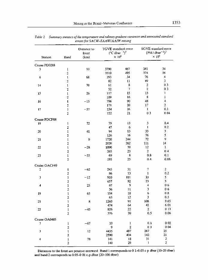
Mean temperature gradient variance estimates (TGVE) and salinity gradient variance estimates (SGVE) corresponding to Subtropical-Subantarctlc mixing in the upper layer are given for two wave number bands (Table 2). In each of the sections analyzed, the highest values of TGVE correspond to the station closest to the front. This feature is common to both bands. In at least 80% of the cases, TGVE and SGVE values are higher for band 1 than for band 2. This characteristic suggests that finestructure processes are more effective in the 10-20 dbar scale than in the 20-100 dbar scale.

A wide range of TGVE variability from 1 x 10 -5 to 1 x 10 -2 (°C dbar-1) 2 is observed. The SGVE varies from 1 x 10 .7 to 1 × 10 -3 (PSU dbar-1) 2. In fact, if for each synoptic section only the station closest to the front is considered, the TGVE is O[10 -3 (°C dbar-1) 2] and the SGVE is O[10 -4 (PSU dbar-1)2]. The lower panels of Fig. 5 (c and d) show the distribution of TGVE and SGVE estimated for the 0.1-0.01 c.p. dbar band plotted versus distance to the front. The variances increase at least by one order of magnitude at distances <20 km to the front. This increase is consistent with the interleaving and mixing expected at the front and indicates that the cross-front variance structure is strongly associated with the large-scale cross-front temperature and salinity fields.

The model of JoYcE (1977) established a relationship between the fine-scale variability of vertical scales in the 10-100 m range and the cross-frontal property fluxes. Assuming a diffusivity of 1 x 10 -4 m 2 s -1 and the estimated cross-front property gradients, the model leads to an averaged cross-front temperature flux of 1 x 10 -2 °C m s -1 and an averaged salinity flux of 1 x 10-3 PSU m s-1. Associated lateral heat and salt diffusivities are of the order 100 m 2 s -1.

Dissipation of eddies and intrusive lenses

Small-scale mixing is also important in the dissipation of intrusive lenses advected across the front. Inspection of all available frontal vertical profiles allows us to estimate roughly the scales of temperature and salinity anomalies and the thickness of the observed intrusions. Temperature anomalies of up to 7°C and salinity anomalies of up to 0.95 PSU are observed (not shown). Based on 30 cases, the maximum thickness of the intrusive layers is 140 m. In this set, mean values of temperature and salinity anomalies and thickness of 2.6°C, 0.35 PSU and 70 m, respectively, were estimated. Given the heat flux calculated for the Brazil-Malvinas Confluence (1.2 x 10-2°C m s-l) , a lens 70 m thick, aspect ratio of 1 x 10 -2 (TooLE and GEORGI, 1981) and temperature anomaly of 2.6°C would be dissipated in 5 to 6 days. Similarly, a salinity anomaly of 0.35 PSU would be dissipated in 1 week. These dissipation timescales are of the same order of magnitude of the estimates available from direct observations of intrusions formed at the shelf/slope water front, south of New England (VOORHIS et al., 1976).

Lateral mixing is also a potential mechanism for dissipation of eddies and meanders that detach from the Confluence downstream of the separation point from the continental slope. In the Austral spring of 1984, a cold and fresh cyclonic eddy of 100 km diameter was observed in the area (GORDON, 1989). The eddy was centered at about 38°S, 52°W and had a mean temperature of 6.5°C and a mean salinity of 34.3 PSU for the upper 400 m. These values lead to a temperature anomaly of 5.3°C and a salinity anomaly of about 0.7 PSU as

0

©

I

©

I I

I

oo

o

o

I I

I I

c~ x~

×~

g~

0

1354 A A BIA/~ etal

compared with the surrounding waters. Based ,1 the order of magnitude of flux estimates due to finestructure, the heat and salt anomal: s would be dissipated in about 6 months. Five months are required to dissipate the heat anomaly, and almost 7 months are required to dissipate the salt anomaly.

The estimate of 6 months should not be interpreted as the mean lifetime of eddies in the region. Obviously, the eddy near-surface properties are subject to alterations associated with the relatively large air-sea fluxes in this region (GORDON, 1981). Furthermore, eddies could re-coalesce with the original water mass prior to its full dissipation by medium-scale mixing.

GORDON (1981, 1989) has observed large alterations in the upper layer thermohaline structure of warm core eddies associated with winter cooling. Early spring SAAW mixed layer warming occurs at a rate of 1-2°C month -~, while cooling of the 200 m thick subtropical mixed layer occurs at a rate of about 0.2°C month -1 (GoRDoN, 1989). It is therefore suggested that the medium-scale mixing due to finestructure is relatively more important than sea-air exchanges in the thermal dissipation of warm core eddies.

Circumpolar Deep Water-North Atlantic Deep Water mixing

Finestructure is also frequently observed at the depth of the deep salinity maximum (2000-3000 m), where NADW mixes with CDW (GEorcI, 1981). The method described before was used to evaluate the lateral heat and salt transfer between CDW and NADW.

Three sections with large lateral temperature-salinity gradients at the deep temperature-salinity maximum (Fig. 1) were identifed. Based on these sections the large- scale mean lateral potential temperature gradient of 3 × 10-6°C m -1 and a salinity gradient of 5.1 × 10 -7 PSU m -1 were estimated. These gradients were estimated from the temperature and salinity differences averaged over a 500 dbar slab centered at o 2 = 36.9.

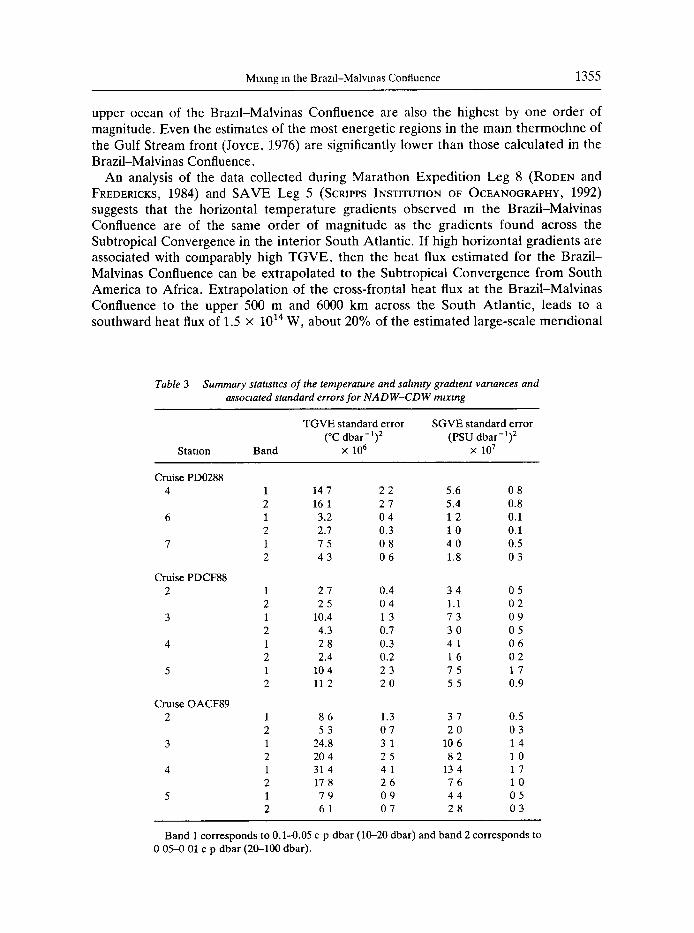
The TGVE and SGVE statistics obtained for the deep water masses are summarized on Table 3. In the three sections it is possible to identify one or more stations with a TGVE of O[10 -5] (°C dbar-a) 2 and SGVE of O[10 -6] (PSU dbar-1) 2. In all cases the standard errors of the estimates are one order of magnitude smaller than the associated variances. Heat and salt vertical diffusivities of 1 x 10 -4 m 2 s -1 lead to heat and salt fluxes of 6.5 × 10-4°C m s -1 and 1.8 x 10 -4 PSU m s -I , respectively.

DISCUSSION

It is useful to compare these results with existing estimates of lateral mixing in other frontal regions of the World Ocean (Table 4). Although the fluxes are related to medium- scale processes, it should be kept in mind that estimates are not based on the same wave- length bands.

Estimates of heat flux for NADW-CDW mixing from GEOR~I (1981) and from this study are in relatively good agreement (Table 4). The large-scale horizontal temperature gradient used by GEOR~I (1981) of 5.0 × 10-6 °C m - 1, is larger than the gradient calculated from the temperature field in this study (3 × 10-6°C m-l) . Thus, the relatively small discrepancy between both estimates is due to differences in the large-scale horizontal temperature gradient. The magnitude of the TGVE, however, remains unchanged.

PIOLA and GEOR~I (1982) computed TGVE at the core of AAIW for different geographic locations (Table 4). They found that the lateral mixing was more intense in the Argentine Basin due to an increased variance in that region. The heat flux estimates for the

Mixing m the Brazf l -Malvmas Confluence 1355

upper ocean of the Brazfl-Malvinas Confluence are also the highest by one order of magnitude. Even the estimates of the most energetic regions in the mam thermochne of the Gulf Stream front (JOYCE, 1976) are significantly lower than those calculated in the Brazil-Malvinas Confluence.

An analysis of the data collected during Marathon Expedition Leg 8 (RooEN and FREDERICKS, 1984) and SAVE Leg 5 (SCRIPPS INSTITUTION OF OCEANOGRAPHY, 1992) suggests that the horizontal temperature gradients observed m the Brazil-Malvinas Confluence are of the same order of magnitude as the gradients found across the Subtropical Convergence in the interior South Atlantic. If high horizontal gradients are associated with comparably high TGVE, then the heat flux estimated for the Brazil- Malvinas Confluence can be extrapolated to the Subtropical Convergence from South America to Africa. Extrapolation of the cross-frontal heat flux at the Brazil-Malvinas Confluence to the upper 500 m and 6000 km across the South Atlantic, leads to a southward heat flux of 1.5 × 1014 W, about 20% of the estimated large-scale merldional

Table 3 Summary stattsttcs of the temperature and sahmty gradtent vartances and assoctated standard errors for N A D W - C D W mtxmg

Statton Band

T G V E standard error S G V E s tandard error (°C dbar-1) 2 (PSU dbar-1) 2

× 10 6 × 10 7

C ~ i s e P D 0 2 8 8 4 1 147 2 2 5.6 0 8

2 161 2 7 5.4 0.8 6 1 3.2 0 4 1 2 0.1

2 2.7 0.3 1 0 0.1 7 1 7 5 0 8 4 0 0.5

2 4 3 0 6 1.8 0 3

Cru i sePDCF88 2 1 2 7 0.4 3 4 0 5

2 2 5 0 4 1.1 0 2 3 1 10.4 1 3 7 3 0 9

2 4.3 0.7 3 0 0 5 4 1 2 8 0.3 4 1 0 6

2 2.4 0.2 1 6 0 2 5 1 104 2 3 7 5 1 7

2 112 2 0 5 5 0.9

C r m s e O A C ~ 9 2 1 8 6 1.3 3 7 0.5

2 5 3 0 7 2 0 0 3 3 1 24.8 3 1 106 1 4

2 2 0 4 2 5 8 2 1 0 4 1 314 4 1 134 1 7

2 178 2 6 7 6 1 0 5 1 7 9 0 9 4 4 0 5

2 6 1 0 7 2 8 0 3

Band 1 corresponds to 0.1--0.05 c p dbar (10-20 dbar) and band 2 corresponds to 0 0 5 - 0 0 1 c p dbar (20-100 dbar).

1356 A A B1ANCHI et al

Table 4 Temperature flux estimates for different frontal regions and water masses

Heat flux Wavelength Region Source (°C m s -1) x 10 -4 band (m)

Polar front (AACC)

Argentine Basra (NADW-CDW)

South of Africa South of New Zealand Argentine Basin (AAIW)

Northwest Atlantic (Gulf Stream)

Brazll-Malvmas (SACW-SAAW) (NADW-CDW)

JOYCE et al (1978)

GEORGI (1981)

PIOLAandGEoRGI (1982)

8 6 3-100

4.0 32-256

2 5 3 4 16--64 9 4

JOYCE (1976) 6.0 2-50

76 0 This study 10-100

6 5

northward heat flux across 30°S in the South Atlantic (Fv, 1981). Thus, 20% of the equatorward large-scale heat flux across 30°S would return poleward in the upper layer of the ocean due to small-scale mixing processes across the Subtropical Convergence.

The small-scale cross-front mixing also may be important in the freshwater balance. There are great uncertainties in the determination of the freshwater fluxes through the sea surface. BAUMGARTNER and REICHEL (1975) have estimated that the net freshwater loss to the atmosphere in the Atlantic north of 30°S is 0.552 x 106 m 3 s- 1. Southward cross-frontal salt flux across the subtropical front in the South Atlantic is required to balance the net excess evaporation north of the front.

Following the criteria established for the heat flux estimates, extrapolation of the medium-scale freshwater flux across the Brazil-Malvinas Confluence to a 500 m slab along the subtropical front in the South Atlantic (6000 km) leads to an integrated southward salt flux of 4 x 106 kg s -1. Assuming that the layer has a mean salinity of 34.8 PSU leads to an integrated freshwater flux of 1.15 x 105 m 3 s -1. Thus, southward salt flux across the Subtropical front of the South Atlantic would account for approximately 20% of the estimated net freshwater loss through the sea surface due to excess evaporation north of the front.

Acknowledgements---Claudia F Gluhvl is supported by Consejo Nacional de Investlgaciones Clentfficas y T6cnicas de la Reptiblica Argentina (CONICET). Cruises PD0284 and OA0485 were financed by U.S. Office of Naval Research contract N000014-84-C-0132 to SiIvia L. Garzoh, Lamont-Doherty Geological Observatory of Columbia University Additional funding for CTD data processing and analysis was provided by CONICET grant 5014365185 to Alberto R. Plola Financial support for cruise PD0288 was provided by Servicio de Hidrograffa Naval of Argentina (SHN) and through NSF grant OCE 87-11529 to Silvia Garzoh Cruises PD0288 and OACF89 were fully financed by SHN The InstltUtO Naclonal de Investlgaci6n y Desarrollo Pesquero made available the fisheries research vessel Captttin Oca Balda for cruise OACF89 after a main engine failure of Puerto Deseado The Instituto Ant~irtlco Argentmo kindly loaned their CTD for use in cruises PDCF88 and OACF89 We wish to acknowledge the officers and crew of A R A. Puerto Deseado and Capttt~n Oea Balda who contributed so much to the success of the field work Marcela Charo and Ana Paula Osiroff were responsible for

Mixing m the Brazll-Malwnas Confluence 1357

processing the CTD data of crmses PD0288, PDCF88 and OACF89 Their patience and good humor were unbeatable

R E F E R E N C E S

BAUMGARTNER A and E REICHEL (1975) The World Water Balance--Mean Annual Global, Continental and Marmrne Preclpztat~on, Evaporatton and Runoff Elsevier, Amsterdam. 179 pp

CHARO M., A. P OSlaOFF, A A BIANCm and A R PIOLA (1991) Datos Ffslco-Qufmlcos, CTD y XBT Campafias Oceanogrfificas: Puerto Deseado 02-88, Confluencla 88 y Confluencla 89. Informe T6cmco no 59/91 Servlclo de Hldrograffa Naval, 450 pp

CHENEY R. E., J G MARSH and B D BECKLEY (1983) Global mesoscale vanabfllty from colhnear tracks of Seasat altimeter data. Journal of Geophyszcal Research, 88, 4343-4354

COt~FLUENCE PPaNClVAL INVESTIGATOaS (1990) Confluence 1988-1990. An intensive study of the southwestern Atlantic. EOS, Transactions, American Geophysical Umon, 71, 1131-1133, 1137

DEACON G. E R (1933) A general account of the hydrology of the South Atlantic Ocean Discovery Reports, 7, 171-238

DEACON G E R (1937) The hydrology of the Southern Ocean. Dtscovery Reports, 15, 1-124 Fu L L (1981) The general circulation and men&onal heat transport of the Subtropical South Atlantic

determined by reverse methods Journal of Physzcal Oceanography, 11, 1171-1193. GARRE'rr C (1979) Mixing in the ocean interior Dynamtcs of Atmospheres and Oceans, 3,239-265 GARZOLI S. L and A. A BIA~Cm (1987) Time-space vanabfllty of the local dynamics of the Brazll-Malvinas

Confluence as revealed by inverted echo sounders Journal of Geophyswal Research, 92, 1914-1922 GEORGI D T (1981) On the relationship between the large-scale property variations and finestructure in the

Circumpolar Deep Water. Journal of Geophysical Research, 86, 6556-6566 GORDON A L. (1981) South Atlantic thermocline ventilation Deep-Sea Research, 28, 1239-1264 GOaDON A. L (1989) Brazd-Malvmas Confluence--1984. Deep-Sea Research, 36, 359-384 GUEgREgO R. A., A A. BXANCm and A. R PmLA (1986) Datos Ffslco-Qufmlcos, C'TD y XBT. Puerto Deseado,

Campafia 02/1984 y Oca Balda, Campafia 04/1985 Servlclo de Hldrografia Naval. Informe T6cmco no 39, 114 pp

JOYCE T M (1976) Large-scale variations m small-scale temperature/sahmty finestructure in the mare thermo- chne of the Northwest Atlantic. Deep-Sea Research, 23, 1175-1186.

JOYCET M (1977)Anoteonthelateralmlxingofwatermasses Journal of Phystcal Oceanography, 7,626-629 JOYCE T M , W. ZENK and J M. TOOLE (1978) The anatomy of the Antarctic Polar Front m the Drake Passage.

Journal of Geophys,cal Research, 83, 6093--6113 LEGECraS R and A GORDON (1982) Satelhte observatmns of the Brazil and Falkland Currents 1975 to 1976 and

1978 Deep-Sea Research, 29,375-401 OLSON D , G PODESTA, R H. EVAt~S and O Bgowlq (1988) Temporal variaUons m the separatmn of Brazil and

Malvmas Currents. Deep-Sea Research, 35, 1971-1990. PATTERSON S L. (1985) Surface circulatmn and kinetic energy &stnbutlons m the southern hemisphere oceans

from FGGE dnftmg buoys. Journal of Physical Oceanography, 15,865-884 PIOLA A R , H A FmUEROA and A A BIANCltl (1987) Some aspects of the surface circulation South of 20°S

revealed by First GARP Global Expenment Drifters Journal of Geophysical Research, 92, 5101-5114 PIOLA A R and O. A GARCi/~ (m press) Atlas oceanogrdfico de la Cuenca Argentina Occzdental y Plataforma

Continental hndera. Servlcm de Hldrograffa Naval, Buenos Aires PIOLA A R. and D T. GEOaGI (1982) Circumpolar properties of Antarctm Intermediate Water and Subantarctlc

Mode Water Deep-Sea Research, 29,687-712 PIOLA A R. and A L GORDON (1989) Intermedmte waters m the southwest South Atlantic. Deep-Sea Research,

36, 1-16 REID J L., W D NOWLIN Ja and W C. PATZERT (1977) On the charactenstlcs and circulation of the

Southwestern Atlantic Ocean. Journal of Physwal Oceanography, 7, 62-91 RODENG I (1986) Thermohaline fronts and barochmc flow m the Argentlne Basm durmg the Austral Sprmg of

1984 Journal of Geophysical Research, 91, 5075-5093 RODEN G I and W. J FREDEVaCKS (1984) Southwest Atlantic Ocean Marathon Expe&tlon, Leg 8, Oct.-Nov

1984 Data Report. Contnbutmn 1637 School of Oceanography, WB-10. University of Washington, Seattle, 436 pp

1358 A A BIANCHI et al

SCRIPPS INSTITUTION of OCEANOGRAPHY (1992) South Atlantic Ventilation Experiment (SAVE) Chemical, Physical and CTD Data Report, Legs 4 and 5, SIO Reference 92-9, ODF Pubhcatlon no 23,625 pp

STERN M (1967) Lateral mixing of water masses Deep-Sea Resea, ch, 14,747-753 SVERDRUP H U., M JOHNSON and R FLEMING (1942) The oceans Thezr phystcs, chemtstry and general btology

Prentice Hall, New York TOOLE J M. and D GEORGI (1981) On the dynamics and effects of double-diffusively driven intrusions Progress

m Oceanography, 10, 123-145 VOORHIS A D., D C. WEBB and R C MILLARD (1976) Current structure and mixing in the shelf/slope water

front south of New England. Journal of Geophyszcal Research, 81, 3695-3708 WOST G (1935) The stratosphere of the Atlantzc Ocean Enghsh translation (1980), W EMERY, e&tor, Amerind

Publishing, New Delhi, 112 pp ZLOTNICKI V. and L. L. Fo (1989) Seasonal variability m global sea level observed with Geosat altimetry Journal

of Geophysical Research, 94, 17,959-17,969