Multiyear measurements of the oceanic and atmospheric boundary

layers at the Brazil-Malvinas confluence region

Luciano Ponzi Pezzi,1 Ronald Buss de Souza,2 Otavio Acevedo,3 Ilana Wainer,4

Mauricio M. Mata,5 Carlos A. E. Garcia,5 and Ricardo de Camargo6

Received 30 October 2008; revised 6 April 2009; accepted 8 June 2009; published 1 October 2009.

[1] This study analyzes and discusses data taken from oceanic and atmosphericmeasurements performed simultaneously at the Brazil-Malvinas Confluence (BMC)region in the southwestern Atlantic Ocean. This area is one of the most dynamical frontalregions of the world ocean. Data were collected during four research cruises in the regiononce a year in consecutive years between 2004 and 2007. Very few studies have addressedthe importance of studying the air-sea coupling at the BMC region. Lateral temperaturegradients at the study region were as high as 0.3�C km�1 at the surface and subsurface. Inthe oceanic boundary layer, the vertical temperature gradient reached 0.08�C m�1 at500 m depth. Our results show that the marine atmospheric boundary layer (MABL) at theBMC region is modulated by the strong sea surface temperature (SST) gradients present atthe sea surface. The mean MABL structure is thicker over the warmside of the BMCwhere Brazil Current (BC) waters predominate. The opposite occurs over the coldside ofthe confluence where waters from the Malvinas (Falkland) Current (MC) are found.The warmside of the confluence presented systematically higher MABL top heightcompared to the coldside. This type of modulation at the synoptic scale is consistent towhat happens in other frontal regions of the world ocean, where the MABL adjusts itselfto modifications along the SST gradients. Over warm waters at the BMC region, theMABL static instability and turbulence were increased while winds at the lower portion ofthe MABL were strong. Over the coldside of the BC/MC front an opposite behavior isfound: the MABL is thinner and more stable. Our results suggest that the sea-levelpressure (SLP) was also modulated locally, together with static stability vertical mixingmechanism, by the surface condition during all cruises. SST gradients at the BMCregion modulate the synoptic atmospheric pressure gradient. Postfrontal and prefrontalconditions produce opposite thermal advections in the MABL that lead to differentpressure intensification patterns across the confluence.

Citation: Pezzi, L. P., R. B. de Souza, O. Acevedo, I. Wainer, M. M. Mata, C. A. E. Garcia, and R. de Camargo (2009), Multiyear

measurements of the oceanic and atmospheric boundary layers at the Brazil-Malvinas confluence region, J. Geophys. Res., 114,

D19103, doi:10.1029/2008JD011379.

1. Introduction

[2] The western region of the South Atlantic Ocean ishighly complex in terms of ocean circulation, water massesformation, and mixing both at the open ocean and at the

coast. The open ocean is modulated by strong mesoscalevariability, mainly dominated by the Brazil Current (BC)and the Malvinas/Falkland Current (MC) at their meetingregion known as the Brazil-Malvinas Confluence (BMC).These currents are characterized by high temporal andspatial variability of the transport, sea surface temperature(SST), chlorophyll concentration, and sea surface height.The BMC region is known as one of the most dynamicallyactive regions of the world ocean [Chelton et al., 1990;Piola and Matano, 2001]. When reaching the BMC region,the tropical/subtropical (warm) waters transported south-ward by the BC interact with the subantarctic (cold) waterstransported by the MC in opposite direction. The mixing ofthese distinct water masses define the western end of thesubtropical convergence in the South Atlantic, a regionknown for the formation and subduction of the SouthAtlantic Central Water (SACW). The last spreads itself allover the South Atlantic Ocean in subsurface layers. In

JOURNAL OF GEOPHYSICAL RESEARCH, VOL. 114, D19103, doi:10.1029/2008JD011379, 2009ClickHere

for

FullArticle

1Earth Observation General Coordination, National Institute for SpaceResearch, Sao Jose dos Campos, Brazil.

2Southern Regional Center for Space Research, National Institute forSpace Research, Santa Maria, Brazil.

3Department of Physics, Federal University of Santa Maria, SantaMaria, Brazil.

4Department of Physical Oceanography, University of Sao Paulo, SaoPaulo, Brazil.

5Ocean and Climate Studies Laboratory, Institute of Oceanography,Federal University of Rio Grande, Rio Grande, Brazil.

6Institute of Astronomy, Geophysics and Atmospheric Sciences,University of Sao Paulo, Sao Paulo, Brazil.

Copyright 2009 by the American Geophysical Union.0148-0227/09/2008JD011379$09.00

D19103 1 of 19

particular locations at tropical regions of the Brazilian coast,depending on the intensity and persistency of the prevailingnortheastern winds, the SACWis upwelled bringing nutrient-rich waters to the continental shelf and promoting theestablishment of well-known phytoplankton blooms [e.g.,Castro et al., 2006].[3] The surface thermal contrasts between distinct water

masses in the ocean are known to contribute toward thegeneration of intense momentum gradients and energyvertical fluxes between the ocean and the atmosphere. Thesefluxes affect the dynamical and thermodynamical structureof both ocean and atmosphere [Chelton et al., 2001;Hashizume et al., 2002; Pezzi et al., 2004, 2005; Tokinagaet al., 2005; Spall, 2007, Small et al., 2008]. In addition tothat, the turbulent processes occurring at small spatial andtemporal scales (order of kilometers and hours) may inducevariations on the evolution of large-scale processes [Pezziand Richards, 2003], at the order of thousands of kilometersand several days. The large-scale processes have directinfluence on themeteorological and oceanographic processesaffecting the South American coastal region [Gan and Rao,1991; Hoskins and Hodges, 2005].[4] Not long ago, Xie [2004], and recently, Small et al.

[2008], have made comprehensive reviews of previousstudies concerning the ocean-atmosphere (OA) interactions.The authors focused especially on areas of strong oceanicfronts such as the equatorial Pacific cold tongue [Chelton etal., 2000; Liu et al., 2000; Polito et al., 2001; Pezzi et al.,2004], the equatorial Atlantic [Hashizume et al., 2001;Caltabiano et al., 2005], and the Southern Ocean [O’Neillet al., 2003]. Those reviews emphasized the necessity tostudy the coupling mechanisms between ocean and atmo-sphere at oceanic frontal regions. The authors pointed outthe fact that over cold waters (where deep atmosphericconvection does not occur), the OA interactions differmarkedly from those occurring over warm waters. In thislast case, many examples taken from Xie [2004] and Smallet al. [2008] describe that the marine atmospheric boundarylayer (MABL) becomes unstable and is deepened overwarm surface waters. The turbulence and the vertical mixingwithin the vertical atmospheric column increases. As aconsequence, the vertical shear decreases, and the surfacewinds become stronger over warm waters. Over colderwaters an opposite situation is observed: the MABL is oftenmore stratified and the surface winds are weaker.[5] In a recent study, Tokinaga et al. [2005] provided a

detailed analysis of the climatological characteristics of thesurface atmospheric stability at the BMC region. Theauthors showed that there is a positive correlation betweenSST and surface wind speed at this region. Their findingswere corroborated by Pezzi et al. [2005], and both areconsistent with the mechanism proposed by Wallace et al.[1989], suggesting that the strong meridional SST gradientbetween BC and MC waters affects the vertical atmosphericmixing. This in turn will affect the MABL stability and willmodulate the winds at lower atmospheric levels.[6] Although the ocean-atmosphere coupling mecha-

nisms, such as the vertical mixing, in the BMC region canbe expected to mirror the behavior of other oceanic regionssuch as the equatorial Pacific and others, no observationaldata of the atmospheric and oceanic mixed layers structure(as well as of air-sea coupling parameters) are currently

available for the BMC region to our knowledge. Anexception to this is the pioneering work of Pezzi et al.[2005]. These last authors presented a description of bothoceanic and atmospheric boundary layers from observationsmade during a single research cruise at the BMC region inNovember 2004. Nevertheless, simultaneous descriptions ofthe synoptic conditions of the MABL and of the oceanicboundary layer (OBL) are still very rare for the BMC regionas well as for the whole of the South Atlantic Ocean.[7] This paper extends the previous work made by Pezzi

et al. [2005] and presents a synoptic description of theMABL and OBL structure as well as the air-sea coupling atthe BMC region. The work is based on in situ data collectedduring four research cruises performed during specific datesin the austral spring from 2004 to 2007. The paper isoutlined as follows: section 2 presents the sampling design,the in situ data, and the applied methodology. A synopticanalysis of the atmosphere and the ocean at the experimen-tal period is made in section 3. The OBL and MABLstructure and the atmospheric adjustment to the oceanicfront are discussed in section 4. The paper finishes with asection presenting our concluding remarks and suggestionsfor future studies.

2. Data and Methods

2.1. In Situ Data Collection

[8] In order to better understand the temporal and spatialvariability of the oceanographic processes and propertiesoccurring in the southwestern Atlantic and their relationshipto the Southern Ocean variability, a research program wasestablished in Brazil in 2002 under the umbrella of theBrazilian Antarctic Program (PROANTAR). Most of theprojects in the field of oceanography were headed by aresearch group called the High Latitudes OceanographyGroup (GOAL). The research group has, among others,the objective of investigating the kinematics and dynamicsof the BMC region and their relation to the Antarctic andSubantarctic environments. The program for measuring andanalyzing the air-sea interactions under the GOAL programis specifically named Air-Sea Interaction at Brazil-MalvinasConfluence (INTERCONF). One of its objectives is theinvestigation of the air-sea coupling in the BMC region andits impact on the weather and climate of the adjacent SouthAmerica coastal regions.[9] During a sequence of INTERCONF cruises during

austral spring, simultaneous oceanic and atmospheric obser-vations were made onboard the Brazilian Navy Oceano-graphic Support Ship (OSS) Ary Rongel while crossing theBMC region. In this study we present an interannualanalysis of the MABL thermal structure mostly based onvertical profiles collected during four cruises between theyears of 2004 to 2007. During the cruises, data for bothMABL and oceanic boundary layer (OBL) were obtainedin the BMC region. The in situ experiments were inspiredby previous works where the air-sea coupling was inves-tigated at oceanic frontal regions in the equatorial Pacific[Hashizume et al., 2002], in Agulhas Current return flow[Rouault et al., 2000], and in the BMC region itself [Pezziet al., 2005; Tokinaga et al., 2005].[10] The OSS Ary Rongel departs from Brazil toward

Antarctica every year during the austral spring. Prior to the

D19103 PEZZI ET AL.: MABL AT THE BRAZIL-MALVINAS CONFLUENCE

2 of 19

D19103

ship’s departure from the port of the Rio Grande city insouthern Brazil, the position of the BC return flow at theBMC region is mapped. The strong surface thermalgradients between BC and MC in the region are deter-mined by satellite imagery and guide the ship toward theregion of maximum thermal gradients between BC andMC (BC/MC front).[11] The study area of the experiments described here is

located between 30� to 50�S and 50� to 60�W (Figure 1).This area was covered during specific dates from 2004 to2007 as indicated in Table 1. While crossing the BC/MCfront, Expendable Bathy-Thermographs (XBTs) werelaunched from the ship in order to measure the watertemperature as a function of depth along the ship’s route.When at the close vicinity of the front (Figure 1 andTable 3), a sequence of Vaisala (RS80 and RS90) radio-sondes were also launched from the rear deck of the ship.The radiosondes measured pressure, temperature, and rela-tive humidity (RH) in the atmosphere. Wind speed anddirection were also estimated from the relative movementof the radiosonde balloon in the atmosphere. The measure-ments were made at regular intervals of 2 s, which guaran-teed a fair number of observations within the MABL, withvertical resolution varying from 7 to 10 m in the firstkilometer of the MABL height. The position of the radio-sonde balloons was traced with the help of a Global PositionSystem (GPS) device onboard of the ship. Other atmosphericvariables were automatically derived by the radiosondereceptor in real time: potential temperature (q), dew pointtemperature (Td), ascension rate, geopotential height, andmixing ratio or specific humidity (q).[12] Before each radiosonde ascent, a ground (onboard)

check was made in order to obtain correction values for theprimary measurements of each radiosonde. During thatcheck, the humidity sensor was placed in a tight sealed drychamber, and the sensor humidity was adjusted to zeropercent. The temperature was measured by an independentthermometer and checked against the radiosonde measure-ment. In situ independent measurements made by the ship’smeteorological station were used to correct for ground checkdifferences. After this procedure, the onboard receptor wassynchronized with the radiosonde, which was attached to aballoon for release. The radiosondes were launched whenthe ship was crossing over from the BC (warm waters) tothe BC/MC front and then to the MC (cold waters),respectively launching as many radiosondes as possible ina period of up to a day. The XBTs were launched simul-taneously with the radiosondes in distances close to aquarter degree latitude.

2.2. Satellite and Atmospheric Data

[13] A number of different data sources were employedover the course of this investigation. As the atmosphericconditions during the experiments were mostly cloudy, thesynoptic thermal surface structure of the BMC region couldnot be observed by infrared imagery. However, satellitemicrowave data from the Advanced Microwave ScanningRadiometer onboard the EOS-Aqua satellite (AMSR-E) wasfully available for the date of the experiments with no cloudcontamination. The Aqua satellite is polar orbiting, offeringa global coverage of the planet.

[14] AMSR-E is a 12-channel passive microwave radi-ometer (6.9, 10.7, 18.7, 23.8, 36.5, and 89.0; vertical andhorizontal polarizations). Raw data is processed into SST atRemote Sensing Systems (RSS) that is a NASA partner fordata processing and distribution. Global AMSR-E SST dataare available on a daily basis at the RSS Web site (http://www.rems.com) as well as wind vectors from the QuikScatscatterometer. Wentz et al. [2003] performed a preliminaryvalidation of the AMSR-E SST against Reynolds OptimumInterpolation (OI) weekly SST. The root mean square error(RMS) differences between AMSR-E and OI SST were0.76�C over a 3-month period spanning from June toAugust 2002. The nominal spatial resolution of the RSSAMSR-E global product is 25 km. A more recent evaluationof the AMSR-E accuracy is presented by Chelton and Wentz[2005].[15] Gridded analysis data from the National Centers for

Environmental Prediction (NCEP) Global Forecast System(GFS) at 1� grid spacing were used for all diagnostics ofthe atmospheric synoptic conditions occurring during theexperiments (e.g., Figure 2). Also, GOES Imager infraredimages for the period of all the experiments (severalimages per day in the period of the study) were obtainedfrom the Brazilian Center for Weather Forecast and Cli-mate Studies (CPTEC, http://www.cptec.inpe.br) and usedin order to complement the synoptic analysis (not shownhere).

2.3. Surface Bulk Flux Calculation and StabilityParameters

[16] From the raw radiosonde data, the turbulent fluxes oflatent heat (QL) and sensible heat (QS) were calculatedfollowing the scheme proposed by Fairall et al. [1996].A comprehensive description of the method is offered bythose authors. The method was developed specifically withthe Tropical Ocean Global Atmosphere–Coupled Ocean-Atmosphere Response Experiment (TOGA-COARE) data.The basic structure of the Fairall et al. [1996] algorithmfollows the well-known Liu-Katsaros-Businger scheme andincludes a different specification to the stress/roughnessrelationship. This approach considers the roughness due tothe gravity waves and molecular viscosity [Smith et al.,1996]. The humidity, temperature, and momentum profilesas a function of the stability under very unstable conditionsare modified to adjust to the Panofsky and Dutton [1984]free convection scheme. The bulk formulas allow thatsensible, latent heat and momentum fluxes can be estimatedfrom the observed variables at 2 or 10 m (reference-levelzr). The basics of this scheme are presented below [Fairallet al., 1996]:

QS ¼ rcpChU qair � SSTð Þ ð1Þ

QL ¼ rLeCeU qs � qairð Þ ð2Þ

where Ch and Ce are the heat and humidity transfercoefficients, which depend on atmospheric stability and aregiven by similarity relationships. qair is the potentialtemperature, qs is the specific humidity at sea level, andqair is the specific humidity at zr. U is the mean speed ofsurface winds relative to the sea surface. All these variables

D19103 PEZZI ET AL.: MABL AT THE BRAZIL-MALVINAS CONFLUENCE

3 of 19

D19103

Figure 1. Brazil-Malvinas Confluence (BMC) study area with cruise routes, radiosonde ascentpositions (black circles), and thermal front positions. QuikScat wind speeds (m s�1) are the linessuperimposed onto AMSR-E sea surface temperature (SST) images. All data are coincident in time withthe experiments. The color bar denotes SST in �C. Experiments are from (a) OP23, (b) OP24, (c) OP25,and (d) OP26 routes.

D19103 PEZZI ET AL.: MABL AT THE BRAZIL-MALVINAS CONFLUENCE

4 of 19

D19103

are measured at zr. In this study we also evaluate the totalheat flux (QT) as given as

QT ¼ QL þ QS ð3Þ

The induced additional flux due to the scale variability ofthe boundary layer and considering the gustiness effect is

also taken into account. The scaling parameter L defined asthe Obukhov length is also calculated by the Fairall et al.[1996] algorithm. According to Stull [1988], the physicalmeaning of this parameter is that L represents the height inthe boundary layer at which buoyant factors first dominateturbulence produced by mechanical factors, e.g., shear. Anatmospheric boundary layer stability parameter at 10-mheight (z) is derived using L:

z ¼ 10=L ð4Þ

where z < 0 means statically unstable (negative) and z > 0means statically stable (positive) conditions.

Table 1. Experiment Names and Dates

Experiment Name Date

OP23 2 to 3 November 2004OP24 28 to 29 October 2005OP25 27 to 28 October 2006OP26 16 to 17 October 2007

Figure 2. Surface synoptic weather analysis, averaged over 0000 and 1200 GMT. Sea-level pressure(hPa) with surface wind (m s�1) vectors superimposed for (a) OP23, 3 November 2004; (b) OP24,28 October 2005; (c) OP25, 16 October 2006; and (d) OP23, 27 October 2007.

D19103 PEZZI ET AL.: MABL AT THE BRAZIL-MALVINAS CONFLUENCE

5 of 19

D19103

[17] It is important to remark that the Fairall et al. [1996]scheme was originally developed to be used on turbulentfluxes over the warm pool in the western Pacific Oceanat the COARE study region. However, Fairall et al.[1996] argues that this scheme has also included extra-tropical data from other research programs. An updateversion of the original algorithm was proposed by Fairallet al. [2003] where the authors present the COAREalgorithm version 3.0. Therefore, this model is consideredto be suitable for extratropical studies as in our case, beingeven used in the past for polar regions [Fairall et al., 1996].The method is largely used by others authors at oceanicfrontal regions, e.g., Rouault et al. [2000] at the AgulhasCurrent.[18] Another parameter widely used for estimating the

near-surface stability is obtained by computing the differencebetween the SST and the near-surface air temperature [Pezziet al., 2005; Tokinaga et al., 2005]. Both variables wereroutinely recorded in shipboard observations. In this work,the stability parameter is defined as SSTbulk � Tship, whereSSTbulk is the bulk-based, in situ manually collected SST bythe OSS Ary Rongel crew along the ship route, and Tship is theair temperature. These observations were collected at enoughspatial and temporal resolutions to allow us the constructionof high-resolution data sets. These data sets were used toinvestigate the MABL stability adjustment to the strongBC/MC front thermal gradients and test the vertical-mixingmechanism. Tship, sea-level pressure (SLP), and RH weremeasured by the meteorological weather station located atthe upper level of the ship, at 11 m above the sea surface.Wind speed measurements (Windship) were made at 22 m.All calculations using the meteorological weather stationdata are hourly averages.

2.4. MABL Composites

[19] The mean MABL structure is described with verticalstructure composites (averages) of the radiosondes profilescalculated using a similar strategy of Pyatt et al. [2005]. Thecomposite method was applied for each transect accom-plished during the four experiments. The radiosonde datawere grouped as a function of their location relative to theSST gradients at the BMC region. Because of the nature ofthe main currents in the area, the warm (cold) waters arealways located northward (southward) of the BC/MC front.For example, during the first experiment (OP23) in thespring of 2004, five radiosondes were launched (Figure 1a).Three of them were released over the warmside of the front,being then used to calculate what we define here as thewarm composite of the MABL vertical structure. The othertwo ascents over the coldside of the front were used to get

the cold composite of the OP23. Warm and cold compositeswere computed for all four experiments.[20] In order to obtain an accurate description of the

vertical structure for this composite analysis, the soundingsmade at the northern (warm) part of the front and at thesouthern (cold) part of the front were independently aver-aged, generating averaged profiles for the warm and coldregions. At each averaged profile, the MABL top height(h0), was subjectively determined using both q and qprofiles. This is the region where the capping inversionlayer or entrainment zone lies. The average h0 values for allexperiments are indicated in Table 2. According to Stull[1988], we can assume that the parameters q and q are wellmixed within the MABL and remain approximately con-stant (adiabatic) in the mixed layer. MABL height dependson the turbulent mixing. A strong gradient of q and q isobserved at higher levels of the atmospheric profile whenthe inversion layer is reached. After that level, the inversionlayer and the h0 are determined by the point when an abruptchange occurs on the profiles, with q increasing and qdecreasing [Fisch et al., 2004]. When this criterion is notmet, Santos [2005] suggests the use of the q profiles todetermine h0 as errors or malfunctions are more common onhumidity sensors than on the temperature ones. A similarapproach is also used by Albrecht et al. [1995]. Over thecoldside of the confluence, especially in cases with warm-air advection, a very stable layer is observed above thesurface. Nevertheless, above this layer, it is possible toobserve a less stable layer, capped by a stronger inversion.In such cases, this upper inversion was considered as theMABL height. The MABL top height determination usingqv was investigated, and it did not show significant differ-ences with respect to calculations using q.[21] The vertical composites were obtained using a non-

dimensional height scale. According to Albrecht et al.[1995] and Pyatt et al. [2005], this procedure preservesthe MABL structure and the inversion height (h0) maincharacteristics even if there are no changes from onesounding to another. This is implemented by normalizingthe radiosondes height (h) by the mean top MABL height ofthe warm and cold portions separately, h0,

h* ¼ h=h0 ð5Þ

[22] This procedure actually transforms h in a nondimen-sional vertical axis (h*). After this step, we look at theaverage profile from the surface to h0 and computedperturbations, which are the differences of each variableto the mean profiles within the MABL. Those mean values

Table 2. Description of Quantities Used in the Radiosonde Profiles Normalization on q, q, and RH Composites Calculation and

Horizontal and Vertical Temperature Gradientsa

OP h0warm h0cold qwarm qcold qwarm qcold DThor DTver

OP23 280 235 17.2 13.0 8.9 6.7 0.03 (39.0�S) 0.08 (39.0�S-400 m)OP24 700 500 10.1 8.6 3.9 3.9 0.03 (39.2�S) 0.09 (39.4�S-400 m)OP25 800 250 14.7 12.6 6.9 6.5 0.05 (38.8�S) 0.07 (39.4�S-400 m)OP26 1060 250 15.2 11.3 7.8 7.6 0.01 (39.8�S) 0.09 (39.6�S-200 m)

aOP is the experiment name. Included are the top marine atmospheric boundary layer (MABL) height for the warm (h0warm) and cold (h0cold) composites;mean MABL potential temperature for the warm (qwarm) and cold (qcold) composites; mean MABL specific humidity for the warm (qwarm) and cold (qcold)composites (units are meters for h, �C for q, and g/kg for q); the horizontal temperature gradient (DThor) at sea surface with the latitude indicated in theparentheses, and the vertical temperature gradient (DTver) with the latitude and depth indicated in parentheses (both gradients are in �C m�1).

D19103 PEZZI ET AL.: MABL AT THE BRAZIL-MALVINAS CONFLUENCE

6 of 19

D19103

were calculated for the cold and warm cases, as seen inTable 2. After that, the composites were calculated as wellas the averaged perturbations of each variable throughoutthe four experiments. The variables were finally restored bymultiplying the vertical coordinate by the mean h0 and thenadding the mean values of each variable to the compositedperturbations. The analysis of the MABL presented here isrestricted to the first 1200 m from the sea surface.

3. Synoptic Analysis

3.1. Oceanic Synoptic Analysis

[23] In order to present a wider view of the oceaniccharacteristics of the study region, the synoptic conditionspresent on the four INTERCONF cruises are shown inFigure 1. Figure 1 shows AMSR-E derived SST fields withnear-surface QuikScat wind vectors superimposed. Thedistribution of the warmer BC waters (in tones rangingfrom yellow to red) and of the colder MC waters (in blue togreen) can be easily seen in the images. The meetinglocation of the opposite Brazil and Malvinas currents isnoticed by strong SST gradient typical of the encounterbetween both currents in the area. The location of the frontin the BMC region responds to the mesoscale variability ofthe confluence as well as the large-scale climatic (atmo-spheric and oceanic) regime which has strong seasonalbehavior [Legeckis and Gordon, 1982].[24] Figure 1 also indicates with black circles the radio-

sonde-launching positions during all cruises. From thesepositions the ship routes crossing the BC/MC front can beapproximately inferred. The tracks representing the ship’sroutes indicate that the BC/MC front was consistentlycrossed at about 39�S to 40�S and 53�W to 54�W. System-atically, in all cruises the SST reached a maximum ofapproximately 20�C over the BC warm core. On the otherhand, the SST values dropped down to values near 5�C overthe cold core of the MC. This remarkable surface SSTgradient is present during the four experiments and agreeswith descriptions made for the BMC by many authors [e.g.,Legeckis and Gordon, 1982; Garcia et al., 2004; Souza etal., 2006]. Another remarkable synoptic characteristic of thestudy area clearly seen in Figure 1 is that the wind speedtends to adjust to the SST field at BC/MC front. Wind speedminima are observed over the cool water at the MC core. Inopposition to that, winds are quite strong away from the MCcore in coastal regions and over the BC warm waters. Thissynoptic pattern of wind modulation agrees with the annualclimatology presented by Tokinaga et al. [2005] for theBMC region.[25] It is also worth remarking that several cyclonic

(clockwise in the southern hemisphere) and anticyclonic(anticlockwise) eddies are continuously shed from the MCand from the BC, respectively. They are three-dimensionalstructures that can easily be identified in SST satelliteimages for their warm (cold) signatures on cold (warm)waters. Vertically, warm (cold) eddies act pushing (pulling)down (up) the thermocline. For instance, Souza et al. [2006]tracked a warm-core eddy shed by the BC in the BMCregion assessing its lifespan and characteristics such as theheat and salt content, as well as the available potentialenergy. As the structures can persist for up to 3 months asthey travel over the mean flow in the southwestern Atlantic,

they are considered an important player on the salt and heatbalance of the region. During the analyzed period it waspossible to identify some of those warm-core structureswhich can be associated to either shedding eddies or themeandering of the BC. It is out of the scope of this study todiscuss the exact classification of those structures here;instead we want to remark that our data suggest that thewind speed over these oceanic features follows the samemodulation pattern described before for the BC/MC frontitself. Very discernable warm-core eddies are found in thestudy area during the OP24, OP25, and OP26 experiments,all centered around 39�S and 53�W. All of these eddies areassociated to stronger winds (9 to 10 m s�1) at theatmosphere over them. On the other hand, weaker windsare noticed over cold-core eddies. This is the case observedduring OP25 where a 6 m s�1 wind speed is estimated overa cold eddy located at 42�S, 51�W.

3.2. Atmospheric Synoptic Analysis

[26] During the OP23 (2–3 November 2004) accordingto onboard observations, the sky was almost fully coveredwith clouds when the radiosondes were released. Theseobserved clouds were mainly associated with instabilitiesproduced by the subtropical jet stream and to a weak trough,both diagnosed by satellite images (not shown) and thesurface synoptic charts seen in Figure 2a. A low-pressuresystem was located in the region between 45�S and 60�W,positioned to the east of the ship’s route. This low pressurewas associated with a weak frontal system that was crossingthe region at the south. A satellite image animation (notshown) and a sea-level pressure chart of the period alsoshowed that the large-scale northerly winds associated to thequasi-permanent Atlantic anticyclone were prevailing overmost of the experiment area. This fact is reinforced by the insitu SLP observations made along the OSS Ary Rongelroute and exhibited in Table 3. The data demonstrate thatthere was not any significant change on the measured SLPvalues compared to the ones measured by the radiosondes.[27] The OP24 (28 October 2005) was performed under

totally cloud covered conditions. This was mostly due to thepresence of a low-pressure system located right over theroute of the OSS Ary Rongel (Figure 2b). Although weak,this system was responsible for the observed cloudinessduring OP24. Even in the presence of this system, the SSTfrontal gradient caused an impact on the SLP of the region.This is better discussed later in section 4.4 of this work (seeFigure 7 and Table 3).[28] During OP25 (27 October 2006), a low pressure with

an associated frontal system was centered over the Malvinas(Falklands) Islands. The frontal system extended northwardto the Malvinas Islands reaching the vicinity of the La PlataRiver. This frontal system was covering a large part of thesampling route of the ship during OP25 (Figure 2c). It isinteresting to note that this experiment had a high-pressuresystem in the vicinity of the ship’s route and a low-pressuresystem to the south of it. Besides the situation observed inthe synoptic chart and satellite imagery of 27 October 2006,this fact is also corroborated by the SLP measurementstaken onboard the ship. The measurements indicate higherSLP values over warmer waters while the opposite occursover cold waters. A similar synoptic situation and SLPbehavior were observed during OP26 (16 October 2007) as

D19103 PEZZI ET AL.: MABL AT THE BRAZIL-MALVINAS CONFLUENCE

7 of 19

D19103

shown in Figure 2d. In this last case, however, the high-pressure system was prevailing over the sampling region.

4. OBL and MABL Observations

4.1. OBL Mean Structure

[29] Figure 3 presents the simultaneous profiles of atmo-spheric potential temperature (q) and ocean temperaturetaken along the route of the OSS Ary Rongel during thefour INTERCONF cruises. Data were taken from thesequences of radiosonde and XBT measurements. Herewe concentrate our analysis in the oceanic part of Figures3a–3d where the temperature data collected with the XBTsare displayed as a function of depth. The OBL verticalstructure shows that the sharp thermal gradients betweenBC and MC extend from the surface to about 500 m depth.These vertical and horizontal gradients characterize the verystrong oceanic front of the BMC region. The estimatedhorizontal (DThor) and vertical (DTver) temperature gra-dients are shown in Table 2. DThor refers to the maximumhorizontal gradient at the surface.DTver displayed in Table 2refers to the maximum vertical gradient found in the BC/MCinterface at depth. The latitude and depth where the maxi-mum gradients were found are also indicated in Table 2.DThor was found to range from 0.01�C m�1 (OP26) to0.05�C m�1 (OP25 at surface and at the vicinity of 39�Swhere the BC/MC front was located). The average gradientis 0.03�C m�1. This value agrees with some early estimates

presented in the literature [e.g., Garzoli and Garraffo, 1989;Saraceno et al., 2004; Souza et al., 2006]. DTver rangedfrom 0.07�C m�1 to 0.09�C m�1 at 400 m depth, approx-imately, in most cases. At our study area, the surfacesubantarctic (MC) waters (colors ranging from blue to greenin Figure 3) meet with the subtropical (BC) waters (colorsranging from yellow to red in Figure 3). At the confluenceof those two water masses, mixing produces the SouthAtlantic Central Water which dives and spreads itself belowthe subtropical waters toward the north. The later watermass is associated to the thermal signature below 500 m inlatitude lower than 39�S (Figure 3). Bianchi et al. [2002]reported the occurrence of a cross-frontal BC/MC interleav-ing, which produces the layering of relatively cold low-salinity waters over warm salty waters. This interleavingmight be playing an important role on the BC/MC front,mixing physical properties by means of small-scale turbu-lent processes. Owing to their very high spatial resolutioncompared to previous hydrographical data presented in theBMC region, our temperature data (Figure 3a) were able toindicate the presence of mesoscale to small-scale structuresat the subsurface in the ocean at the BC/MC front. Thesestructures are particularly noticeable at approximately39.5�S, confined to the first 400 m depth. In this case,some interleaving is clearly noticeable between the watersin the region. Pezzi and Richards [2003] demonstrated thestrong influence of the lateral mixing enhancement at thevicinity of the equator in the Pacific Ocean. The physical

Table 3. Experiments Name, Date, and Locations of the Radiosondes Ascenta

OP Date Time (LT) Lat (S) Lon (W) SSTSat Tair SLPRad WindRad WindSat

OP23 2 November 2004 1930 38.12 53.55 17.40 19.40 1010.0 10.00 8.802 November 2004 2130 38.43 53.68 17.10 16.50 1007.0 10.00 9.003 November 2004 0022 39.00 53.89 16.65 18.00 1006.0 7.00 9.203 November 2004 0220 39.54 54.11 13.20 11.00 1007.0 5.00 8.803 November 2004 0518 40.01 54.30 9.75 10.00 1008.0 7.00 5.80

OP24 28 October 2005 0232 38.63 52.58 16.65 15.00 1009.0 10.00 7.6028 October 2005 0329 38.76 52.68 16.95 14.00 1008.0 6.00 7.2028 October 2005 0451 38.95 52.82 17.25 14.00 1008.0 7.00 7.4028 October 2005 0714 39.27 53.02 16.65 12.00 1008.0 5.00 7.0028 October 2005 0811 39.42 53.15 14.70 12.00 1010.0 5.00 6.4028 October 2005 0916 39.60 53.26 12.60 10.00 1010.0 5.00 5.6028 October 2005 1024 39.77 53.36 11.40 14.50 1009.0 4.00 5.8028 October 2005 1201 40.00 53.50 10.95 15.00 1010.0 4.00 6.6028 October 2005 1322 40.04 53.52 10.95 15.00 1010.0 4.00 6.6028 October 2005 1421 40.18 53.61 10.95 15.00 1010.0 4.00 6.6028 October 2005 1619 40.35 53.82 11.10 14.00 1010.0 4.00 7.0028 October 2005 1746 40.54 54.03 11.25 11.50 1010.0 4.00 7.20

OP25 27 October 2006 1101 38.51 53.51 13.80 17.50 1014.2 13.00 8.2027 October 2006 1351 38.73 53.00 17.55 18.00 1016.0 5.00 9.4027 October 2006 1502 38.86 53.27 15.15 20.00 1015.0 6.00 8.8027 October 2006 1615 38.94 53.53 12.75 20.00 1015.0 6.00 7.6027 October 2006 1812 39.14 53.99 10.20 13.50 1013.0 3.60 5.6027 October 2006 1913 39.23 54.20 9.15 13.00 1013.0 4.10 5.4027 October 2006 2104 39.40 54.60 8.70 13.00 1012.0 5.10 4.6027 October 2006 2247 39.55 54.95 8.55 10.00 1012.0 5.10 4.4028 October 2006 0022 39.68 55.26 8.70 10.00 1012.0 8.20 4.2028 October 2006 0153 39.81 55.57 8.40 10.00 1011.0 8.20 4.00

OP26 16 October 2007 0512 39.52 54.50 13.05 11.00 1015.0 8.70 6.4016 October 2007 0706 39.68 54.62 13.05 14.00 1013.0 10.00 6.4016 October 2007 0806 39.81 54.77 10.65 14.00 1013.0 9.00 5.6016 October 2007 0852 39.93 54.91 8.85 12.00 1010.0 10.00 4.60

aThe variables are air temperature (Tair) in �C, sea-level pressure (SLPRad) in hPa, and wind speed (WindRad) in m s�1. Data collected by the radiosondeson all experiments. AMSR-E sea surface temperature (SSTSat) and QuikScat wind speed (WindSat) are satellite data measurements approximatelycoincident with the radiosondes ascent time and positions. Note that Tair is the first-level radiosonde data.

D19103 PEZZI ET AL.: MABL AT THE BRAZIL-MALVINAS CONFLUENCE

8 of 19

D19103

reasoning to which they have been based for explaining thisenhanced mixing was the effect of the observed interleavingof water masses in producing a meridional flux of tracers

and momentum at oceanic fronts [Richards and Edwards,2003]. Although this process is likely to occur in the BMCas well, further study is necessary to better investigate the

Figure 3. Temperature profiles (K) of the atmosphere and ocean taken simultaneously by radiosondesand XBTs along the OSS Ary Rongel’s routes during the four experiments OP23, OP24, OP25, andOP26. Meridional wind vectors (m s�1) are also displayed. The profiles are for (a) 3 November 2004,(b) 28 October 2005, (c) 16 October 2006, and (d) 27 October 2007.

D19103 PEZZI ET AL.: MABL AT THE BRAZIL-MALVINAS CONFLUENCE

9 of 19

D19103

characteristics and impacts of these small-scale features inthe BMC zone.

4.2. MABL Mean Structure

[30] The thermal structure of the MABL, as measured bythe radiosondes for each cruise, is displayed in the upperhalf of Figures 3a–3d. Figure 3 displays the atmospheric

potential temperature (q) together with the meridional windalso estimated from radiosonde data. Generally, at the southof the BC/MC front location, the air temperature is lowerthan at the north. Figure 3 clearly shows that MABL isbeing influenced by the OBL temperature distribution. Overthe warm waters, we observe strong winds with an unstablemixed layer. On this side of the front, a reduction in the

Figure 3. (continued)

D19103 PEZZI ET AL.: MABL AT THE BRAZIL-MALVINAS CONFLUENCE

10 of 19

D19103

wind shear and a decrease in the static stability of the near-surface atmosphere are also seen. Over the coldside of thefront, on the other hand, the MABL is more stable, the windshear is stronger, and the surface winds are weaker. Thosesignatures are consistent with the mechanism proposed byWallace et al. [1989]. Still over cold waters, the atmospherepresents an increased vertical wind shear and a weakeningof the surface winds. Our analysis shows that this verticalmixing mechanism occurring in the BMC region at synoptictime scale is in close agreement with the climatologydescribed by Tokinaga et al. [2005]. Nearly all aspects ofthe ocean-atmosphere coupling observed in our results arealso in agreement with previous studies made for otheroceanic frontal regions, such as the eastern equatorialPacific [Wallace et al., 1989; Hayes et al., 1989; Cheltonet al., 2001; Hashizume et al., 2002; Pezzi et al., 2004;Small et al., 2005; Spall, 2007]. It is worth mentioning thatthe atmosphere at the BMC region responds to the strongSST gradients with a consequent strong horizontal thermalgradient (Figure 3). The radiosonde wind data is also inclose agreement with the surface winds estimated fromQuikScat measurements (Figure 2). The satellite-derivedwinds indicated that during three out of our four experi-

ments (OP24 is an exception), a predominant northerlymeridional component was present along the ship’s trackwhere our in situ data were taken. Southern winds domi-nated the area during OP24. This information is crucial forunderstanding the mean characteristics of the MABL acrossthe BC/MC front at BMC region. Distinct air temperatureadvection patterns take place depending whether the large-scale winds are blowing from the cold toward the warmregion, or vice versa.[31] Now we turn our attention to analyzing the vertical

MABL structure as a function of the SST bottom boundarycondition. Aiming for that objective, we use all radiosondedata collected in the four experiments. Figures 4a–4ddisplay the composite calculations based on radiosondevertical profiles of q, q, RH, wind magnitude, and u and vwind components. The RH profiles were divided by 101 inorder to plot q values in the same order of magnitude. Theanalyses presented here are restricted to the first 1200 m ofheight from the sea surface. These results are helpful tobetter understand the atmosphere characteristics as a func-tion of the lower boundary surface. The composites of theatmosphere over warm waters (Figures 4a and 4b) show awell-defined convective MABL structure, including the top

Figure 4. Vertical composite profiles of potential temperature (q), specific humidity (q), and relativehumidity (RH) for (a) warm and (b) cold cases. Vertical composite profiles of Wind speed (wnd) andzonal (u) and meridional (v) wind components for (c) warm and (d) cold cases.

D19103 PEZZI ET AL.: MABL AT THE BRAZIL-MALVINAS CONFLUENCE

11 of 19

D19103

height (h0). The observed changes seen in the compositesdisplayed in Figures 4a and 4c are consistent with the SSTchanges observed from the warmside to the coldside of thefront. Figure 4a indicates that the MABL top was located atapproximately 600 m. This feature is noticeable in both qand q profiles. The humidity is well mixed at the warmregion and does not present a strong vertical gradient. Astrong thermal (q) inversion occurs between 600 m and800 m, after which a softer gradient is observed up to about1600 m. At the lower levels inside the MABL, q remainsalmost constant with respect to height owing to the verticalturbulent mixing. In this case, a well-developed mixed layertakes place. The specific humidity decreases with heightabove h0 (�600 m). This decrease is less intense than thatof q.[32] Figures 4c and 4d show interesting features of the

vertical composite profiles calculated over the coldside ofthe BMC region. These profiles display a lower MABL topwith capping inversion at �300 m height, where theatmosphere is becoming dryer (�60% of RH). At lowerlevels the RH is between 70% and 80%. Above theinversion level, q remains almost constant up to a secondaryinversion level, which is detected at 700 m. The verticalstructure of the inversions described here is observed in theRH and qe profiles. These profiles indicate a strong reduc-tion of moisture, which originates at the sea surface andascends toward the MABL. This fact suggests that the upperMABL is decoupled from the surface layer. Hashizume etal. [2002] observed a similar pattern over cold waters at theeastern equatorial Pacific. It should be noted that the qprofile cannot be used alone to clearly characterize theMABL top at our study region.[33] Figures 4b and 4d show the composites of the

vertical distribution of the zonal (u) and meridional (v)wind speed for the warmsides and coldsides of the BMCregion. Figures 4b and 4d show that for both sides of theBC/MC front, the v component is negative indicating a windflowing from the north along the whole of the MABL. Theu component of the wind is positive at both sides of thefront, indicating that westerly winds prevail. A minimumoccurs at the surface. Near the surface, the northerlydirection prevails on v. Above 400 m, the westerly directiondominates the u component of the wind. The larger magni-tude of the northerly winds indicates that the large-scalesynoptic circulation mostly prevailed during the period ofour observations. For instance, Figure 2 shows that thesurface northerly wind direction seen along the ship’s routeis associated to the high-pressure (anticyclonic) circulationpresent during OP23, OP25, and OP26. The meridionalwinds have larger magnitude compared to the zonal windsat BMC region. At the warm region of the oceanic front, theu component (and consequently the wind speed) is strongerat the surface when compared with the cold region (Figures4b and 4d). Above 400 m, this situation is reversed: the ucomponent (and wind speed) is weaker at the warm partof the front when compared to the cold part. This was notthe case for v, which is strong throughout the whole ofthe MABL. The meridional component is high at both thewarm and cold regions from the surface (�4.4 m s�1 and�4.2 m s�1, respectively) up to 1200 m (�5.0 m s�1 and�1.6 m s�1, respectively). A stronger vertical wind shearnear the surface is seen in the v component profiles of the

cold-case composites. A less accentuated wind shear ispresent in the zonal component of the wind for both warmand cold cases. However, the vertical wind shear is moreaccentuated for the zonal when compared to the meridionalcomponent of the wind. These patterns indicate that thecoldside of the BMC region presents a larger static stability.As a consequence, there is less mixing, and a more stratifiedMABL develops. This layer presents a stronger verticalshear at lower atmospheric levels compared to the warmpart of the BMC region. At this warm region, the wind shearis less accentuated producing a more turbulent and mixedMABL.

4.3. Near-Surface Fluxes

[34] The collected data by the ship-borne meteorologicalstation of OSS Ary Rongel were used to estimate the surfaceturbulent flux calculations. Measured SSTbulk, Windship,Tship, SLP, and RH are also included in the analysis here.Negative values of the heat fluxes indicate fluxes from thesea surface toward the atmosphere. The atmospheric bound-ary layer stability parameter at 10 m height (z) wasmultiplied by 102.[35] Figures 5 and 6 show the near-surface data and

estimates for all the particular experiments (OP23 toOP26). The wind speed displays some common featuresof variability from year to year as seen in Figure 5. On thenorthernmost part of the domain, the wind speed presentsvalues ranging from 5 m s�1 (OP24 and OP26) to 15 m s�1

(OP25). After this starting point, wind speeds begin togradually increase when the air is lying over the BC(warmside) and near to the BMC oceanic front. Themaximum wind speed values at the BC side range from11 m s�1 (OP26) to 23 m s�1 (OP25). All measurementsshow that wind speed tends to decrease fairly slowly whilecrossing the BC/MC front (denoted by the vertical line inthe graph) and when over the colder waters at the MCdomain. In some cases an abrupt decline in wind speed isobserved (as in OP23). The wind speed has dropped downfrom 10 m s�1 to 6 m s�1. At the cold BMC side themaximum wind speeds vary from 5 m s�1 registered inOP23 to 11 m s�1 in OP25. It is interesting to note that inOP25 even over cold waters the wind speed has increasedsouthward of the BC/MC front. This could be due to thelarge-scale circulation phenomena rather than the local SSTmodulation. However, even with this increase the windspeed is still small compared to that of the warm BC/MCside. It is more intense over the northern part of the domain,where the warm waters are located. Over the cold waters,the wind is less intense, so the reduction in wind stress isassociated to the air-sea uncoupling under stable profiles asseen in section 5.2. This fact is also confirmed through thestability indexes analyses later in this section.[36] The near-surface stability parameter SSTbulk � Tship

clearly shows in Figure 5 that sea surface temperatureaffects the MABL near-surface stability. This parametershows positive values over the warmside of the BC/MCfront, meaning that the sea surface is acting as a heat sourceto the atmosphere. At the coldside, the opposite situationoccurs. A colder ocean than the near-surface air allows amore stable MABL. In particular, the colder surface waterwill induce the formation of a stable mixed layer thatdecouples the upper MABL (as discussed in section 4.2)

D19103 PEZZI ET AL.: MABL AT THE BRAZIL-MALVINAS CONFLUENCE

12 of 19

D19103

indicating a reduction of the vertical mixing. The near-surface stability conditions verified in this analysis are alsoverified by z calculations. The z results have negative(positive) values north (south) of the BC/MC confluence,which points to unstable (stable) conditions of the loweratmosphere. The spatial distribution of z is in reasonableagreement with the SSTbulk � Tship calculations.[37] The total heat fluxes vary approximately from�215 W m�2 to 50 W m�2. These estimates, as well astheir spatial variability, are in fair agreement with theclimatology presented by Tokinaga et al. [2005]. For allexperiments the maximum QT estimates are distributedbetween 35�S and 39�S, for all QS, QL, and QT, approxi-mately. The larger fluxes values found at the warmside areassociated with the larger air-sea temperature differencesand wind speeds occurring at this region (see also Table 3).

This feature is characteristic of the region where the MABLis unstable and flux exchanges are intense. Conversely, atthe coldside of the confluence, QT is reduced to valuesranging from �20 W m�2 (OP24) to 60 W m�2 (OP25).This reduction is also associated with the lower SST andwind speed found in this region (Figures 5 and 7). DuringOP25 and OP26 the energy fluxes at the coldside of theoceanic front were directed downward. During these twoexperiments, northerly winds blew at the confluence, drivinga warm-air advection toward the south and then creating avery stable boundary layer at the coldside.[38] The mean fluxes estimated over the warmside of the

BMC are generally higher than those obtained on thecoldside. As it should be expected, the warmside releasesmore energy toward the atmosphere because of the higherSST and stronger wind speed, driving a more unstable

Figure 5. Synoptic, in situ measurements taken along OSS Ary Rongel routes for (a) OP23, (b) OP24,(c) OP25, and (d) OP26. (Windship): wind speed measured at the vessel; (SSTbulk � Tship) stabilityparameters (�C); QT: total heat fluxes (�10 W m�2); z: atmospheric stability parameter (�102). Allinformation is derived from the ship-borne meteorological data. The vertical lines denote approximatelythe Brazil Current (BC)/Malvinas (Falkland) Current (MC) front position.

D19103 PEZZI ET AL.: MABL AT THE BRAZIL-MALVINAS CONFLUENCE

13 of 19

D19103

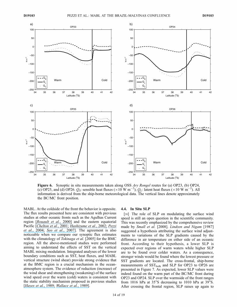
MABL. At the coldside of the front the behavior is opposite.The flux results presented here are consistent with previousstudies at other oceanic fronts such as the Agulhas Currentregion [Rouault et al., 2000] and the eastern equatorialPacific [Chelton et al., 2001; Hashizume et al., 2002; Pezziet al., 2004; Seo et al., 2007]. The agreement is alsonoticeable when we compare our synoptic flux estimateswith the climatology of Tokinaga et al. [2005] for the BMCregion. All the above-mentioned studies were performedaiming to understand the effects of SST on the verticalMABL mixing modulation. Integrated analyses of the lowerboundary conditions such as SST, heat fluxes, and MABLvertical structure (wind shear) provide strong evidence thatat the BMC region is a crucial mechanism in the ocean-atmosphere system. The evidence of reduction (increase) ofthe wind shear and strengthening (weakening) of the surfacewind speed over the warm (cold) waters is consistent withthe static stability mechanism proposed in previous studies[Hayes et al., 1989; Wallace et al., 1989].

4.4. In Situ SLP

[39] The role of SLP on modulating the surface windspeed is still an open question in the scientific community.This was recently emphasized by the comprehensive reviewmade by Small et al. [2008]. Lindzen and Nigam [1987]suggested a hypothesis attributing the surface wind adjust-ments to variations of the SLP gradients caused by thedifference in air temperature on either side of an oceanicfront. According to their hypothesis, a lower SLP isexpected over regions of warm waters while higher SLPare to be found over colder waters. As a consequence,stronger winds would be found where the lowest pressure orSST gradients are located. The cross-frontal, ship-bornemeasurements of SSTbulk and SLP for OP23 to OP26 arepresented in Figure 7. As expected, lower SLP values wereindeed found on the warm part of the BC/MC front duringOP23 and OP24. SLP over the warmside of the front rangesfrom 1016 hPa at 35�S decreasing to 1010 hPa at 39�S.After crossing the frontal region, SLP raises up again to

Figure 6. Synoptic in situ measurements taken along OSS Ary Rongel routes for (a) OP23, (b) OP24,(c) OP25, and (d) OP26. QS: sensible heat fluxes (�10 W m�2); QL: latent heat fluxes (�10 W m�2). Allinformation is derived from the ship-borne meteorological data. The vertical lines denote approximatelythe BC/MC front position.

D19103 PEZZI ET AL.: MABL AT THE BRAZIL-MALVINAS CONFLUENCE

14 of 19

D19103

1006 hPa near 41�S. During OP25 and OP26, however, theSLP presented an opposite behavior. High pressure occursover the warmside of the front with values ranging from1017 hPa (OP25) up to 1022 hPa (OP26). Over the cold-side, SLP drops down to 1011 hPa and 1005 hPa for OP25and OP26, respectively. These data, measured by thebarometer onboard the ship (Figure 7), are confirmed bythe radiosonde data (Table 3).[40] Most of the observed SLP changes across the con-

fluence are, in fact, determined by the synoptic configura-tion of the atmosphere. Figure 2 shows a broader-scalepattern. Nevertheless, the questions about how much of thehydrostatic MABL adjustments are caused by the local SSTmodulation or by the synoptic scale systems still remain. Inorder to complement our analysis, we plotted smoothedlatitude-height contours of the pressure perturbation indi-vidually for each expedition (Figure 8). At each level, theaverage pressure was removed, and then a ‘‘perturbationpressure’’ was computed with respect to the horizontalpressure average.[41] In all cases except OP24 a reasonably large pressure

gradient exists above the boundary layer, with higherpressure observed at lower latitudes (the warm sector).

Furthermore, all cases show an appreciable perturbation ofthe pressure gradient within the boundary layer. Thisperturbation is generally more intense at lower levels,indicating that it must be associated to surface-relatedprocesses. Besides these general agreements, some aspectsare remarkably different among each of the experiments.During OP23, the confluence was responsible for weaken-ing the pressure gradient within the boundary layer. In OP25and OP26, on the other hand, the synoptic pressure gradientwas intensified within the boundary layer. In OP24, despitethe subtle synoptic pressure gradient, a well-defined pres-sure gradient induced by the oceanic front occurs within theboundary layer, with higher pressures at the coldside.[42] Tomas et al. [1999] report that the MABL pressure

perturbation beyond the synoptic forcing depends on twoprocesses. First, the SST difference tends to generate lowerpressures over the warmer side of the oceanic front and viceversa. However, the warmside boundary layer also tends tobe thicker as noticed in our results (Figure 4a), beingconsequently denser than the free atmosphere air over adeeper column that occurs over the coldside. This processtends to induce higher pressures over the warm sector.Therefore, the final result will depend on which of the two

Figure 7. Synoptic, in situ measurements taken along OSS Ary Rongel routes for (a) OP23, (b) OP24,(c) OP25, and (d) OP26. SLP, sea-level pressure measured at the vessel; SST, sea surface temperature(�C). The vertical line approximately denotes the BC/MC front position.

D19103 PEZZI ET AL.: MABL AT THE BRAZIL-MALVINAS CONFLUENCE

15 of 19

D19103

processes is dominant. Song et al. [2006] and Skyllingstadet al. [2007] both suggested that in extratropical regions(such as the BMC), the boundary layer structure over anoceanic front will largely depends on the existing thermaladvection pattern of the atmosphere.[43] In the case of cold-air advection (cold air coming

from the south of the BC/MC front) during our experiments,a mixed layer occurs at the coldside of the front. Theadvected cold air enhances the vertical air temperaturegradients and, consequently, the sensible heat fluxes overthe warmside of the front. This configuration results in athicker, warmer boundary layer over the warm sectorcompared to that of the cold sector. Such a configuration,with cold-air advection across the confluence, for instance,happened during OP24. In this case, the coldside mixedlayer was approximately 500 m thick, with a mean potentialtemperature of 281.75 K. Over the warmside of the oceanicfront, the mixed layer was 700 m high, associated to a meanpotential temperature of 283.25 K (Table 2). Such temper-ature difference over a moderately deep boundary layer isenough to dominate over the influence caused by thethickness effect. Therefore, the cold-air advection, prevalentin OP24, is responsible for positive (negative) pressureperturbations over the coldside (warmside) of the BMC. A

similar process occurred during OP23. In that case, thepressure perturbations locally induced at the BMC opposethe existing synoptic pressure gradient, reducing it at lowerlevels.[44] In contrast, when warm-air advection (warm air

coming from the north of the BC/MC front) exists acrossthe BMC region, the mixed layer exists only over the warmsector. In the cold portion, a shallow, highly stable boundarylayer is produced as a consequence of downward sensibleheat fluxes. Despite being appreciably colder than the warmportion, such a stable boundary layer is shallower than themixed layer occurring over the warmside. In that case, thethickness effect dominates over the atmospheric tempera-ture effect, and the SST gradients are responsible forpositive (negative) pressure perturbations over the warmside(coldside) of the BC/MC front. Cases of warm-air advectionwere observed during OP25 and OP26, when northwardmeridional winds prevailed. In both cases, the pressureperturbation enhanced the existent synoptic gradient, asshown in Figure 8.[45] In a large-eddy simulations study, Skyllingstad et al.

[2007] investigated the flow across an oceanic front for bothcases of cold and warm thermal advection. Their resultsconfirm the description above made for our observations. In

Figure 8. Smoothed latitude-height contours of pressure perturbation for the four experiments OP23,OP24, OP25, and OP26. The perturbations are determined with respect to the average pressure at eachheight. Contour units are in hPa.

D19103 PEZZI ET AL.: MABL AT THE BRAZIL-MALVINAS CONFLUENCE

16 of 19

D19103

a warm-air advection case, a negative pressure perturbationoccurs over the cold portion of an oceanic front. Inopposition to that, a cold-air advection determines a positivepressure perturbation over the cold portion. Skyllingstad etal. [2007], however, do not explain their pattern differences,but Tomas et al. [1999] clarifies the issue. In conclusion, ourobservations, together with the theory proposed by Tomaset al. [1999] and the numerical simulations by Skyllingstadet al. [2007] comprise a good set of evidence to demon-strate how thermal advection drives a pressure gradientacross oceanic fronts. For emphasizing that conclusion, avery simple conceptual model can be inferred, directlyassociating the type of advection to the sign of the pressureperturbation across the BC/MC front.

5. Concluding Remarks

[46] This work analyzed and discussed simultaneousoceanic and atmospheric data collected during four experi-ments carried out by the INTERCONF program at the BMCregion. This work extends and complements the study ofPezzi et al. [2005] where only data from November 2005were available. To our knowledge, this is the only systematicobservational ocean-atmosphere sampling effort conductedat the Brazil-Malvinas Confluence region so far. Despite thefact that this region is acknowledged as one of the mostenergetic regions of the world ocean, very few studies haveaddressed the importance of studying the air-sea couplingprocesses there. Our results indicate the presence of lateralSST gradients at BMC as high as 0.3�C km�1 at surface andsubsurface. Vertical water temperature gradients are on theorder of 0.08�C m�1 at depths of 400–500 m.[47] Analyzing the MABL-OBL coupling during four

cruises between 2004 and 2007, this work offered elementsto conclude that the MABL is modulated by the strongtemperature gradients present at the sea surface of the studyarea. An explanation for this modulation lies in the fact thatthe MABL in the BMC region adjusts itself to the SSTmodifications characteristic from oceanic frontal regions, asalready reported for other areas of the world ocean such asthe equatorial Pacific and the Agulhas Current region. Overwarm waters, the static instability and the turbulence withinthe MABL are both increased. Still over warm waters, ourdata indicated a reduction in the wind shear as well as anenhancement of the surface winds at the MABL. Over thecoldside of the BMC region, the MABL is more stable andis associated to an increased wind shear, resulting in weakersurface winds. Both situations are in close agreement withresults presented by Wallace et al. [1989] for the easternequatorial Pacific Ocean. This process was already pro-posed as an explanation for the air-sea coupling at otherfrontal regions of the world ocean as described in the veryrecent review paper by Small et al. [2008]. For our studyregion, the mean MABL structure was thicker over thewarmside (BC) than over the coldside (MC) of the conflu-ence. The warmside displayed systematically larger h0values compared to the coldside. The surface QS and QL

fluxes always increased from the cold to the warmside of theoceanic front owing to the increase of the wind and temper-ature (q) difference between the sea surface and the air.[48] Some interesting points arose from the results of our

observational effort. Our analysis suggests that the SLP was

locally modulated the surface condition during all experi-ments. The static stability vertical mixing mechanismexplains this modulation. This was clearly observed inOP23 and OP24, where lower (higher) SLP values arelocated over warm (cold) waters (Figures 7a and 7b). Nev-ertheless, the BMC SST gradients also modulated the syn-optic pressure gradient observed during OP25 and OP26.However, in these last cases, the SLP leaded an opposite role,driving lower pressures at the coldside and higher pressuresat the warmside. Different results are reported by de Szoekeand Bretherton [2004] and Small et al. [2005]. For addressingthis issue, we should bear in mind that the southwesternAtlantic Ocean is a cyclone and anticyclone track region[Hoskins and Hodges, 2005]. This fact distinguishes thisregion from most of better previously studied frontal oceanicregions, which are located in the tropics. We suggest that thepresence of large scale synoptic system affects the SLPmodulation at the Brazil-Malvinas Confluence region. Theeffects of postfrontal and prefrontal conditions can result inopposite advective patterns of the atmosphere in the region.[49] To better investigate all these complex interactions

between the local and the large-scale processes, oceanic andatmospheric models should be employed. Numerical mod-eling can complement our observational results in thefuture, as well as being useful for directing new experimentstoward particular regions of our study area. Both de Szoekeand Bretherton [2004] and Small et al. [2005] offered asimilar approach for studying the equatorial Pacific Ocean.Long numerical integrations (e.g., seasonal simulationscovering a large scale) may permit us to isolate the effectsof the large-scale signals from the local SST one, and thenwe can check whether the hydrostatic stability is a relevantplayer in the MABL stability process when a synopticsystem is active over the BMC region or, on the other hand,it is negligible compared to the large-scale (pressure) signal.[50] We finish by remarking that the southwestern Atlan-

tic Ocean is a very important region for the weather andclimate of South America, since it is a path for atmosphericfrontal and storm tracks and cyclone generation and inten-sification. We expect that new, consistent efforts to betterstudy and understand the air-sea coupling in the BMCregion can benefit from the results presented here. It isexpected that, in the future, a continuous observing programfor studying the air-sea coupling processes in the south-western Atlantic region can be established.

[51] Acknowledgments. We thank Maria Assuncao F. Silva Dias andAntonio Divino Moura for the scientific input. Three anonymous reviewersprovided comments which reflected substantial improvements to this paper.Paulo Arlino is acknowledged for his support in the field. Radiosondeswere provided by CPTEC/INPE and INMET. AOML/NOAA and theBrazilian Navy provided the XBTs. We are especially thankful to the OSSAry Rongel crew and scientists for their help and support during all cruises.We also thank the Brazilian Inter-Ministerial Committee for the Resources ofthe Sea (CIRM) and the Brazilian Ministry of the Environment (MMA) fortheir support to GOAL activities. This research was funded by grants2005/02359-0 (OCATBM-FAPESP), 550370/2002-1 (GOAL), 557284/2005-8 (INTERCONF), and 520189/2006-0 (SOS-CLIMATE) of CNPq/PROANTAR. This is also a first author contribution for the PQ andUniversal (CNPq) project numbers 306670/2006-2 and 476971/2007-1.

ReferencesAlbrecht, B. A., M. P. Jensen, and W. J. Syrett (1995), Marine boundarylayer structure and fractional cloudiness, J. Geophys. Res., 100,14,209–14,222.

D19103 PEZZI ET AL.: MABL AT THE BRAZIL-MALVINAS CONFLUENCE

17 of 19

D19103

Bianchi, A. A., A. R. Piola, and G. J. Collino (2002), Evidence of doublediffusion in the Brazil-Malvinas Confluence, Deep Sea Res., Part I, 49,41–52, doi:10.1016/S0967-0637(01)00039-5.

Caltabiano, A. C., I. S. Robinson, and L. Pezzi (2005), Multi-year satelliteobservations of instability waves in the tropical Atlantic Ocean, OceanSci. Disc., 2, 1–35.

Castro, B. M., J. A. Lorenzzetti, I. C. A. Silveira, and L. B. Miranda (2006),Estrutura termohalina e circulacao na regiao entre o Cabo de Sao Tome(RJ) e o Chuı (RS), in O ambiente oceanografico da plataformacontinental e do talude na regiao Sudeste-Sul do Brasil, edited byC. L. del Bianco Rossi-Wongtschowski and L. Saint-Pastous Madureira,pp. 11–120, EDUSP, Sao Paulo, Brazil.

Chelton, D. B., and F. J. Wentz (2005), Global microwave satellite obser-vations of sea-surface temperature for numerical weather prediction andclimate research, Bull. Am. Meteorol. Soc., 86, 1097–1115, doi:10.1175/BAMS-86-8-1097.

Chelton, D. B., M. G. Schlax, D. L. Witter, and J. G. Richman (1990),GEOSAT altimeter observations of the surface circulation of theSouthern Ocean, J. Geophys. Res., 95, 17,877–17,903, doi:10.1029/JC095iC10p17877.

Chelton, D. B., F. J. Wentz, C. L. Gentemann, R. A. de Szoeke, and M. G.Schlax (2000), Satellite microwave SST observations of transequatorialtropical instability waves, Geophys. Res. Lett., 27(9), 1239–1242,doi:10.1029/1999GL011047.

Chelton, D. B., S. K. Esbensen, M. G. Schlax, N. Thun, M. Freilich,F. J. Wentz, C. L. Gentmann, M. J. McPhaden, and P. S. Schopf (2001),Observations of coupling between surface wind stress and sea surfacetemperature in the eastern tropical Pacific, J. Clim., 14, 1479–1498,doi:10.1175/1520-0442(2001)014<1479:OOCBSW>2.0.CO;2.

de Szoeke, S. P., and C. S. Bretherton (2004), Quasi-Lagrangian large eddysimulation of cross-equatorial flow in the East Pacific atmosphericboundary layer, J. Atmos. Sci., 61, 1837–1858, doi:10.1175/1520-0469(2004)061<1837:QLESOC>2.0.CO;2.

Fairall, C. W., E. F. Bradley, D. P. Rogers, J. B. Edson, and G. S. Young(1996), Bulk parameterization of air-sea fluxes for Tropical Ocean-GlobalAtmosphere Coupled-Ocean Atmosphere Response Experiment, J. Geo-phys. Res., 101, 3747–3764, doi:10.1029/95JC03205.

Fairall, C. W., E. F. Bradley, J. E. Hare, A. A. Grachev, and J. B. Edson(2003), Bulk parameterization of air-sea fluxes: Updates and verificationfor the COARE algorithm, J. Clim., 16, 571–591, doi:10.1175/1520-0442(2003)016<0571:BPOASF>2.0.CO;2.

Fisch, G., J. Tota, L. A. T. Machado, M. A. F. Silva Dias, R. F. da F. Lyra,C. A. Nobre, A. J. Dolman, and J. H. C. Gash (2004), The convectiveboundary layer over pasture and forest in Amazonia, Theor. Appl.Climatol., 78(1–3), 47–59, doi:10.1007/s00704-004-0043-x.

Gan, M. A., and V. B. Rao (1991), Surface cyclogenesis over SouthAmerica, Mon. Weather Rev., 119, 1293–1302, doi:10.1175/1520-0493(1991)119<1293:SCOSA>2.0.CO;2.

Garcia, C. A. E., Y. V. B. Sarma, M. M. Mata, and V. M. T. Garcia (2004),Chlorophyll variability and eddies in the Brazil-Malvinas Confluenceregion, Deep Sea Res., 51, 159–172, doi:10.1016/j.dsr2.2003.07.016.

Garzoli, S. L., and Z. Garraffo (1989), Transports, frontal motions andeddies at the Brazil-Malvinas Currents confluence, Deep Sea Res., PartA, 36, 681–703, doi:10.1016/0198-0149(89)90145-3.

Hashizume, H., S. P. Xie, W. T. Liu, and K. Takeuchi (2001), Local andremote atmospheric response to tropical instability waves: A global viewfrom space, J. Geophys. Res., 106, 10,173 – 10,185, doi:10.1029/2000JD900684.

Hashizume, H., S.-P. Xie, M. Fujiwara, M. Shiotani, T. Watanabe,Y. Tanimoto, W. T. Liu, and K. Takeuchi (2002), Direct observations ofatmospheric boundary layer response to SST variations associated withtropical instability waves over the eastern equatorial Pacific, J. Clim.,15 , 3379 – 3393, do i :10.1175/1520-0442(2002)015<3379:DOOABL>2.0.CO;2.

Hayes, S. P., M. J. McPhaden, and J. M. Wallace (1989), The influence ofsea surface temperature on surface wind in the eastern equatorial Pacific:Weekly to monthly variability, J. Clim., 2, 1500–1506, doi:10.1175/1520-0442(1989)002<1500:TIOSST>2.0.CO;2.

Hoskins, B. J., and K. I. Hodges (2005), A new perspective on SouthernHemisphere storm tracks, J. Clim., 18, 4108 – 4129, doi:10.1175/JCLI3570.1.

Legeckis, R., and A. L. Gordon (1982), Satellite observations of theBrazil and Falkland Currents: 1975 to 1976 and 1978, Deep SeaRes., 29, 375–401, doi:10.1016/0198-0149(82)90101-7.

Lindzen, R. S., and S. Nigam (1987), On the role of sea surface temperaturegradients in forcing low-level winds and convergence in the tropics,J. Atmos. Sci., 44(17), 2418–2436, doi:10.1175/1520-0469(1987)044<2418:OTROSS>2.0.CO;2.

Liu, W., X. Xie, P. S. Polito, S. P. Xie, and H. Hashizume (2000),Atmospheric manifestation of tropical instability wave observed by

QuickSCAT and tropical rain measuring mission, Geophys. Res. Lett.,27(16), 2545–2548, doi:10.1029/2000GL011545.

O’Neill, L. W., D. B. Chelton, and S. K. Esbensen (2003), Observations ofSST-induced perturbations of the wind stress field over the SouthernOceanon seasonal time scales, J. Clim., 16, 2340–2354, doi:10.1175/2780.1.

Panofsky, H., and J. A. Dutton (1984), Atmospheric Turbulence, 397 pp.,Wiley-Intersci., New York.

Pezzi, L. P., and K. J. Richards (2003), Effects of lateral mixing on themean state and eddy activity of an equatorial ocean, J. Geophys. Res.,108(C12), 3371, doi:10.1029/2003JC001834.

Pezzi, L. P., J. Vialard, K. J. Richards, C. Menkes, and D. Anderson (2004),Influence of ocean atmosphere coupling on the properties of tropical instabil-ity waves, Geophys. Res. Lett., 31, L16306, doi:10.1029/2004GL019995.

Pezzi, L. P., R. B. Souza, M. S. Dourado, C. A. E. Garcia, M. M. Mata, andM. A. F. Silva-Dias (2005), Ocean-atmosphere in situ observations at theBrazil-Malvinas Confluence region, Geophys. Res. Lett., 32, L22603,doi:10.1029/2005GL023866.

Piola, A. R., and R. P. Matano (2001), Brazil and Falklands (Malvinas)currents, in Encyclopedia of Ocean Sciences, edited by S. A. Thorpe,pp. 340–349, Elsevier, New York.

Polito, P., J. P. Ryan, W. T. Liu, and F. P. Chavez (2001), Oceanic atmo-spheric anomalies of tropical instability waves, Geophys. Res. Lett.,28(11), 2233–2236, doi:10.1029/2000GL012400.

Pyatt, H. E., B. A. Albrecht, C. Fairall, J. E. Hare, N. Bond, P. Minnis, andJ. K. Ayers (2005), Evolution of marine atmospheric boundary layerstructure across the Cold Tongue– ITCZ Complex, J. Clim., 18,737–753, doi:10.1175/JCLI-3287.1.

Richards, K. J., and N. Edwards (2003), Lateral mixing in the equatorialPacific: The importance of inertial instability, Geophys. Res. Lett., 30(17),1888, doi:10.1029/2003GL017768.

Rouault, M., A. M. Lee-Thorp, and Lutjeharms (2000), The atmosphericboundary layer above the Agulhas Current during alongcurrent winds,J. Phys. Oceanogr., 30, 40–50, doi:10.1175/1520-0485(2000)030<0040:TABLAT>2.0.CO;2.

Santos, L. A. R. (2005), Analise e carcterizacao da camada limite convec-tiva em area de pastagem, durante o perıodo de transicao entre a estacaosea e chuvosa na Amazonia (Experimento RaCCI-LBA), 118 pp., INPE-551.5510.522. M. Sci. Diss. in Meteorol., INPE, Sao Jose dos Campos,Brazil.

Saraceno, M., C. Provost, A. R. Piola, J. Bava, and A. Gagliardini (2004),Brazil Malvinas Frontal System as seen from 9 years of advanced veryhigh resolution radiometer data, J. Geophys. Res., 109, C05027,doi:10.1029/2003JC002127.

Seo, H., M. Jochum, R. Murtugudde, A. J. Miller, and J. O. Roads (2007),Feedback of tropical instability-wave-induced atmospheric variabilityonto the ocean, J. Clim., 20, 5842–5855, doi:10.1175/JCLI4330.1.

Skyllingstad, E. D., D. Vickers, L. Mahrt, and R. Samelson (2007), Effectsof mesoscale sea surface temperature fronts on the marine atmosphericboundary layer, Boundary Layer Meteorol., 123, 219–237, doi:10.1007/s10546-006-9127-8.

Small, R. J., S.-P. Xie, Y. Wang, S. K. Esbensen, and D. Vickers (2005),Numerical simulation of boundary layer structure and cross-equatorialflow in the eastern Pacific, J. Atmos. Sci., 62, 1812–1830, doi:10.1175/JAS3433.1.

Small, R. J., S. P. de Szoeke, S. P. Xie, L. O’Neill, H. Seo, Q. Song,P. Cornillon, M. Spall, and S. Minobe (2008), Air-sea interaction overocean fronts and eddies, Dyn. Atmos. Oceans, 45, 274–319, doi:10.1016/j.dynatmoce.2008.01.001.

Smith, S. D., C. W. Fairall, G. L. Geernaert, and L. Hasse (1996), Air-seafluxes: 25 years of progress, Boundary Layer Meteorol., 78, 247–290,doi:10.1007/BF00120938.

Song, Q., P. Cornillon, and T. Hara (2006), Surface wind response to oceanicfronts, J. Geophys. Res., 111, C12006, doi:10.1029/2006JC003680.

Souza, R. B., M. M. Mata, C. A. E. Garcia, M. Kampel, E. N. Oliveira, andJ. A. Lorenzzetti (2006), Multi-sensor satellite and in situ measure-ments of a warm core eddy south of the Brazil-Malvinas Conflu-ence region, Remote Sens. Environ., 100, 52 – 66, doi:10.1016/j.rse.2005.09.018.

Spall, M. A. (2007), Effect of sea surface temperature-wind stresscoupling on baroclinic instability in the ocean, J. Phys. Oceanogr.,37, 1092–1097, doi:10.1175/JPO3045.1.

Stull, R. B. (1988), An Introduction to Boundary Layer Meteorology, 666pp., Kluwer Acad. Publ., Dordrecht, Netherlands.

Tomas, R. A., J. R. Holton, and P. J. Webster (1999), The influence of cross-equatorial pressure gradients on the location of near-equatorial convection,Q. J. R. Meteorol. Soc., 125, 1107–1127, doi:10.1256/smsqj.55602.

Tokinaga, H., Y. Tanimoto, and S.-P. Xie (2005), SST-induced wind varia-tions over Brazil-Malvinas confluence: Satellite and in-situ observations,J. Clim., 18, 3470–3482, doi:10.1175/JCLI3485.1.

D19103 PEZZI ET AL.: MABL AT THE BRAZIL-MALVINAS CONFLUENCE

18 of 19

D19103

Wallace, J. M., T. P. Mitchell, and C. J. Deser (1989), The influence of sea-surface temperature on surface wind in the eastern equatorial Pacific:Weekly to monthly variability, J. Clim., 2, 1492–1499, doi:10.1175/1520-0442(1989)002<1492:TIOSST>2.0.CO;2.

Wentz, F. J., C. Gentemann, and P. Ashcroft (2003), On-orbit calibrationof AMSR-E and the retrieval of ocean products, 83rd AMS AnnualMeeting, Am. Meteorol. Soc., Long Beach, Calif., 9–13 February.

Xie, S. P. (2004), Satellite observations of cool ocean-atmosphereinteraction, Bull. Am. Meteorol. Soc., 85, 195–208, doi:10.1175(BAMS-82–2-195).

�����������������������O. Acevedo, Department of Physics, UFSM, Campus da UFSM, Avenida

Roraima 1000, Camobi Caixa Postal 5021, Santa Maria, CEP 97105-970,Brazil.

R. de Camargo, IAG, USP, Rua do Matao 1226, Sao Paulo, CEP 05508-090, Brazil.R. B. de Souza, CRS, INPE, Campus da UFSM, Avenida Roraima 1000,

Camobi Caixa Postal 5021, Santa Maria, CEP 97105-970, Brazil.C. A. E. Garcia and M. M. Mata, Ocean and Climate Studies Laboratory,

Institute of Oceanography, FURG, Avenida Italia Km 08, Rio Grande,96201-900, Brazil.L. P. Pezzi, OBT, INPE, Avenida dos Astronautas 1758, Jardim da

Granja, Sao Jose dos Campos, 12227-010, Brazil. (luciano@dsr.inpe.br)I. Wainer, Department of Physical Oceanography, USP, Praca do

Oceanografico 191, Sao Paulo, 05508-120, Brazil.

D19103 PEZZI ET AL.: MABL AT THE BRAZIL-MALVINAS CONFLUENCE

19 of 19

D19103