
Technological approaches to linguistic documentation and meta-documentation
Upload
khangminh22Category
view
4download
0
GROMACSGroningen Machine for Chemical Simulations
Reference ManualVersion 2018.5


GROMACSReference Manual
Version 2018.5
Contributions from
Emile Apol, Rossen Apostolov, Herman J.C. Berendsen,Aldert van Buuren, Pär Bjelkmar, Rudi van Drunen,Anton Feenstra, Sebastian Fritsch, Gerrit Groenhof,
Christoph Junghans, Jochen Hub, Peter Kasson,Carsten Kutzner, Brad Lambeth, Per Larsson, Justin A. Lemkul,
Viveca Lindahl, Magnus Lundborg, Erik Marklund, Pieter Meulenhoff,Teemu Murtola, Szilárd Páll, Sander Pronk,
Roland Schulz, Michael Shirts, Alfons Sijbers,Peter Tieleman, Christian Wennberg and Maarten Wolf.
Mark Abraham, Berk Hess, David van der Spoel, and ErikLindahl.
c© 1991–2000: Department of Biophysical Chemistry, University of Groningen.Nijenborgh 4, 9747 AG Groningen, The Netherlands.
c© 2001–2019: The GROMACS development teams at the Royal Institute of Technology andUppsala University, Sweden.
More information can be found on our website: www.gromacs.org.

iv
Preface & Disclaimer
This manual is not complete and has no pretention to be so due to lack of time of the contributors– our first priority is to improve the software. It is worked on continuously, which in some casesmight mean the information is not entirely correct.
Comments on form and content are welcome, please send them to one of the mailing lists (seewww.gromacs.org), or open an issue at redmine.gromacs.org. Corrections can also be made in theGROMACS git source repository and uploaded to gerrit.gromacs.org.
We release an updated version of the manual whenever we release a new version of the software,so in general it is a good idea to use a manual with the same major and minor release number asyour GROMACS installation.
On-line Resources
You can find more documentation and other material at our homepage www.gromacs.org. Amongother things there is an on-line reference, several GROMACS mailing lists with archives andcontributed topologies/force fields.
Citation information
When citing this document in any scientific publication please refer to it as:
M.J. Abraham, D. van der Spoel, E. Lindahl, B. Hess, and the GROMACSdevelopment team, GROMACS User Manual version 2018.5, www.gromacs.org(2019)
However, we prefer that you cite (some of) the GROMACS papers [1, 2, 3, 4, 5, 6, 7, 8] whenyou publish your results. Any future development depends on academic research grants, since thepackage is distributed as free software!
GROMACS is Free Software
The entire GROMACS package is available under the GNU Lesser General Public License (LGPL),version 2.1. This means it’s free as in free speech, not just that you can use it without pay-ing us money. You can redistribute GROMACS and/or modify it under the terms of the LGPLas published by the Free Software Foundation; either version 2.1 of the License, or (at youroption) any later version. For details, check the COPYING file in the source code or consulthttp://www.gnu.org/licenses/old-licenses/lgpl-2.1.html.
The GROMACS source code and and selected set of binary packages are available on our home-page, www.gromacs.org. Have fun.
Contents
1 Introduction 1
1.1 Computational Chemistry and Molecular Modeling . . . . . . . . . . . . . . . . 1
1.2 Molecular Dynamics Simulations . . . . . . . . . . . . . . . . . . . . . . . . . . 2
1.3 Energy Minimization and Search Methods . . . . . . . . . . . . . . . . . . . . . 5
2 Definitions and Units 7
2.1 Notation . . . . . . . . . . . . . . . . . . . . . . . . . . . . . . . . . . . . . . . 7
2.2 MD units . . . . . . . . . . . . . . . . . . . . . . . . . . . . . . . . . . . . . . 7
2.3 Reduced units . . . . . . . . . . . . . . . . . . . . . . . . . . . . . . . . . . . . 9
2.4 Mixed or Double precision . . . . . . . . . . . . . . . . . . . . . . . . . . . . . 10
3 Algorithms 11
3.1 Introduction . . . . . . . . . . . . . . . . . . . . . . . . . . . . . . . . . . . . . 11
3.2 Periodic boundary conditions . . . . . . . . . . . . . . . . . . . . . . . . . . . . 11
3.2.1 Some useful box types . . . . . . . . . . . . . . . . . . . . . . . . . . . 13
3.2.2 Cut-off restrictions . . . . . . . . . . . . . . . . . . . . . . . . . . . . . 14
3.3 The group concept . . . . . . . . . . . . . . . . . . . . . . . . . . . . . . . . . 14
3.4 Molecular Dynamics . . . . . . . . . . . . . . . . . . . . . . . . . . . . . . . . 15
3.4.1 Initial conditions . . . . . . . . . . . . . . . . . . . . . . . . . . . . . . 17
3.4.2 Neighbor searching . . . . . . . . . . . . . . . . . . . . . . . . . . . . . 18
3.4.3 Compute forces . . . . . . . . . . . . . . . . . . . . . . . . . . . . . . . 24
3.4.4 The leap-frog integrator . . . . . . . . . . . . . . . . . . . . . . . . . . 26
3.4.5 The velocity Verlet integrator . . . . . . . . . . . . . . . . . . . . . . . 26
3.4.6 Understanding reversible integrators: The Trotter decomposition . . . . . 27
3.4.7 Multiple time stepping . . . . . . . . . . . . . . . . . . . . . . . . . . . 29
3.4.8 Temperature coupling . . . . . . . . . . . . . . . . . . . . . . . . . . . 29

vi Contents
3.4.9 Pressure coupling . . . . . . . . . . . . . . . . . . . . . . . . . . . . . . 35
3.4.10 The complete update algorithm . . . . . . . . . . . . . . . . . . . . . . 42
3.4.11 Output step . . . . . . . . . . . . . . . . . . . . . . . . . . . . . . . . . 42
3.5 Shell molecular dynamics . . . . . . . . . . . . . . . . . . . . . . . . . . . . . . 44
3.5.1 Optimization of the shell positions . . . . . . . . . . . . . . . . . . . . . 44
3.6 Constraint algorithms . . . . . . . . . . . . . . . . . . . . . . . . . . . . . . . . 45
3.6.1 SHAKE . . . . . . . . . . . . . . . . . . . . . . . . . . . . . . . . . . . 45
3.6.2 LINCS . . . . . . . . . . . . . . . . . . . . . . . . . . . . . . . . . . . 46
3.7 Simulated Annealing . . . . . . . . . . . . . . . . . . . . . . . . . . . . . . . . 48
3.8 Stochastic Dynamics . . . . . . . . . . . . . . . . . . . . . . . . . . . . . . . . 49
3.9 Brownian Dynamics . . . . . . . . . . . . . . . . . . . . . . . . . . . . . . . . 50
3.10 Energy Minimization . . . . . . . . . . . . . . . . . . . . . . . . . . . . . . . . 50
3.10.1 Steepest Descent . . . . . . . . . . . . . . . . . . . . . . . . . . . . . . 50
3.10.2 Conjugate Gradient . . . . . . . . . . . . . . . . . . . . . . . . . . . . . 51
3.10.3 L-BFGS . . . . . . . . . . . . . . . . . . . . . . . . . . . . . . . . . . . 51
3.11 Normal-Mode Analysis . . . . . . . . . . . . . . . . . . . . . . . . . . . . . . . 51
3.12 Free energy calculations . . . . . . . . . . . . . . . . . . . . . . . . . . . . . . 52
3.12.1 Slow-growth methods . . . . . . . . . . . . . . . . . . . . . . . . . . . 52
3.12.2 Thermodynamic integration . . . . . . . . . . . . . . . . . . . . . . . . 54
3.13 Replica exchange . . . . . . . . . . . . . . . . . . . . . . . . . . . . . . . . . . 55
3.14 Essential Dynamics sampling . . . . . . . . . . . . . . . . . . . . . . . . . . . . 56
3.15 Expanded Ensemble . . . . . . . . . . . . . . . . . . . . . . . . . . . . . . . . . 57
3.16 Parallelization . . . . . . . . . . . . . . . . . . . . . . . . . . . . . . . . . . . . 57
3.17 Domain decomposition . . . . . . . . . . . . . . . . . . . . . . . . . . . . . . . 57
3.17.1 Coordinate and force communication . . . . . . . . . . . . . . . . . . . 58
3.17.2 Dynamic load balancing . . . . . . . . . . . . . . . . . . . . . . . . . . 58
3.17.3 Constraints in parallel . . . . . . . . . . . . . . . . . . . . . . . . . . . 60
3.17.4 Interaction ranges . . . . . . . . . . . . . . . . . . . . . . . . . . . . . . 60
3.17.5 Multiple-Program, Multiple-Data PME parallelization . . . . . . . . . . 61
3.17.6 Domain decomposition flow chart . . . . . . . . . . . . . . . . . . . . . 63
3.18 Implicit solvation . . . . . . . . . . . . . . . . . . . . . . . . . . . . . . . . . . 63
4 Interaction function and force fields 67
4.1 Non-bonded interactions . . . . . . . . . . . . . . . . . . . . . . . . . . . . . . 67

Contents vii
4.1.1 The Lennard-Jones interaction . . . . . . . . . . . . . . . . . . . . . . . 68
4.1.2 Buckingham potential . . . . . . . . . . . . . . . . . . . . . . . . . . . 69
4.1.3 Coulomb interaction . . . . . . . . . . . . . . . . . . . . . . . . . . . . 70
4.1.4 Coulomb interaction with reaction field . . . . . . . . . . . . . . . . . . 70
4.1.5 Modified non-bonded interactions . . . . . . . . . . . . . . . . . . . . . 71
4.1.6 Modified short-range interactions with Ewald summation . . . . . . . . . 73
4.2 Bonded interactions . . . . . . . . . . . . . . . . . . . . . . . . . . . . . . . . . 73
4.2.1 Bond stretching . . . . . . . . . . . . . . . . . . . . . . . . . . . . . . . 74
4.2.2 Morse potential bond stretching . . . . . . . . . . . . . . . . . . . . . . 75
4.2.3 Cubic bond stretching potential . . . . . . . . . . . . . . . . . . . . . . 75
4.2.4 FENE bond stretching potential . . . . . . . . . . . . . . . . . . . . . . 76
4.2.5 Harmonic angle potential . . . . . . . . . . . . . . . . . . . . . . . . . . 76
4.2.6 Cosine based angle potential . . . . . . . . . . . . . . . . . . . . . . . . 77
4.2.7 Restricted bending potential . . . . . . . . . . . . . . . . . . . . . . . . 78
4.2.8 Urey-Bradley potential . . . . . . . . . . . . . . . . . . . . . . . . . . . 79
4.2.9 Bond-Bond cross term . . . . . . . . . . . . . . . . . . . . . . . . . . . 79
4.2.10 Bond-Angle cross term . . . . . . . . . . . . . . . . . . . . . . . . . . . 79
4.2.11 Quartic angle potential . . . . . . . . . . . . . . . . . . . . . . . . . . . 79
4.2.12 Improper dihedrals . . . . . . . . . . . . . . . . . . . . . . . . . . . . . 80
4.2.13 Proper dihedrals . . . . . . . . . . . . . . . . . . . . . . . . . . . . . . 81
4.2.14 Tabulated bonded interaction functions . . . . . . . . . . . . . . . . . . 84
4.3 Restraints . . . . . . . . . . . . . . . . . . . . . . . . . . . . . . . . . . . . . . 86
4.3.1 Position restraints . . . . . . . . . . . . . . . . . . . . . . . . . . . . . . 86
4.3.2 Flat-bottomed position restraints . . . . . . . . . . . . . . . . . . . . . . 87
4.3.3 Angle restraints . . . . . . . . . . . . . . . . . . . . . . . . . . . . . . . 88
4.3.4 Dihedral restraints . . . . . . . . . . . . . . . . . . . . . . . . . . . . . 88
4.3.5 Distance restraints . . . . . . . . . . . . . . . . . . . . . . . . . . . . . 89
4.3.6 Orientation restraints . . . . . . . . . . . . . . . . . . . . . . . . . . . . 92
4.4 Polarization . . . . . . . . . . . . . . . . . . . . . . . . . . . . . . . . . . . . . 96
4.4.1 Simple polarization . . . . . . . . . . . . . . . . . . . . . . . . . . . . . 96
4.4.2 Anharmonic polarization . . . . . . . . . . . . . . . . . . . . . . . . . . 96
4.4.3 Water polarization . . . . . . . . . . . . . . . . . . . . . . . . . . . . . 97
4.4.4 Thole polarization . . . . . . . . . . . . . . . . . . . . . . . . . . . . . 97
4.5 Free energy interactions . . . . . . . . . . . . . . . . . . . . . . . . . . . . . . . 97

viii Contents
4.5.1 Soft-core interactions . . . . . . . . . . . . . . . . . . . . . . . . . . . . 100
4.6 Methods . . . . . . . . . . . . . . . . . . . . . . . . . . . . . . . . . . . . . . . 102
4.6.1 Exclusions and 1-4 Interactions. . . . . . . . . . . . . . . . . . . . . . . 102
4.6.2 Charge Groups . . . . . . . . . . . . . . . . . . . . . . . . . . . . . . . 103
4.6.3 Treatment of Cut-offs in the group scheme . . . . . . . . . . . . . . . . 103
4.7 Virtual interaction sites . . . . . . . . . . . . . . . . . . . . . . . . . . . . . . . 104
4.8 Long Range Electrostatics . . . . . . . . . . . . . . . . . . . . . . . . . . . . . 107
4.8.1 Ewald summation . . . . . . . . . . . . . . . . . . . . . . . . . . . . . . 107
4.8.2 PME . . . . . . . . . . . . . . . . . . . . . . . . . . . . . . . . . . . . 108
4.8.3 P3M-AD . . . . . . . . . . . . . . . . . . . . . . . . . . . . . . . . . . 109
4.8.4 Optimizing Fourier transforms and PME calculations . . . . . . . . . . . 110
4.9 Long Range Van der Waals interactions . . . . . . . . . . . . . . . . . . . . . . 110
4.9.1 Dispersion correction . . . . . . . . . . . . . . . . . . . . . . . . . . . . 110
4.9.2 Lennard-Jones PME . . . . . . . . . . . . . . . . . . . . . . . . . . . . 112
4.10 Force field . . . . . . . . . . . . . . . . . . . . . . . . . . . . . . . . . . . . . . 115
4.10.1 GROMOS-96 . . . . . . . . . . . . . . . . . . . . . . . . . . . . . . . . 115
4.10.2 OPLS/AA . . . . . . . . . . . . . . . . . . . . . . . . . . . . . . . . . . 116
4.10.3 AMBER . . . . . . . . . . . . . . . . . . . . . . . . . . . . . . . . . . 116
4.10.4 CHARMM . . . . . . . . . . . . . . . . . . . . . . . . . . . . . . . . . 117
4.10.5 Coarse-grained force fields . . . . . . . . . . . . . . . . . . . . . . . . . 117
4.10.6 MARTINI . . . . . . . . . . . . . . . . . . . . . . . . . . . . . . . . . . 118
4.10.7 PLUM . . . . . . . . . . . . . . . . . . . . . . . . . . . . . . . . . . . 118
5 Topologies 119
5.1 Introduction . . . . . . . . . . . . . . . . . . . . . . . . . . . . . . . . . . . . . 119
5.2 Particle type . . . . . . . . . . . . . . . . . . . . . . . . . . . . . . . . . . . . . 119
5.2.1 Atom types . . . . . . . . . . . . . . . . . . . . . . . . . . . . . . . . . 120
5.2.2 Virtual sites . . . . . . . . . . . . . . . . . . . . . . . . . . . . . . . . . 120
5.3 Parameter files . . . . . . . . . . . . . . . . . . . . . . . . . . . . . . . . . . . 122
5.3.1 Atoms . . . . . . . . . . . . . . . . . . . . . . . . . . . . . . . . . . . . 122
5.3.2 Non-bonded parameters . . . . . . . . . . . . . . . . . . . . . . . . . . 122
5.3.3 Bonded parameters . . . . . . . . . . . . . . . . . . . . . . . . . . . . . 123
5.4 Molecule definition . . . . . . . . . . . . . . . . . . . . . . . . . . . . . . . . . 124
5.4.1 Moleculetype entries . . . . . . . . . . . . . . . . . . . . . . . . . . . . 124

Contents ix
5.4.2 Intermolecular interactions . . . . . . . . . . . . . . . . . . . . . . . . . 125
5.4.3 Intramolecular pair interactions . . . . . . . . . . . . . . . . . . . . . . 125
5.4.4 Exclusions . . . . . . . . . . . . . . . . . . . . . . . . . . . . . . . . . 126
5.5 Implicit solvation parameters . . . . . . . . . . . . . . . . . . . . . . . . . . . . 126
5.6 Constraint algorithms . . . . . . . . . . . . . . . . . . . . . . . . . . . . . . . . 127
5.7 pdb2gmx input files . . . . . . . . . . . . . . . . . . . . . . . . . . . . . . . . . 128
5.7.1 Residue database . . . . . . . . . . . . . . . . . . . . . . . . . . . . . . 129
5.7.2 Residue to building block database . . . . . . . . . . . . . . . . . . . . . 131
5.7.3 Atom renaming database . . . . . . . . . . . . . . . . . . . . . . . . . . 131
5.7.4 Hydrogen database . . . . . . . . . . . . . . . . . . . . . . . . . . . . . 132
5.7.5 Termini database . . . . . . . . . . . . . . . . . . . . . . . . . . . . . . 133
5.7.6 Virtual site database . . . . . . . . . . . . . . . . . . . . . . . . . . . . 135
5.7.7 Special bonds . . . . . . . . . . . . . . . . . . . . . . . . . . . . . . . . 136
5.8 File formats . . . . . . . . . . . . . . . . . . . . . . . . . . . . . . . . . . . . . 137
5.8.1 Topology file . . . . . . . . . . . . . . . . . . . . . . . . . . . . . . . . 137
5.8.2 Molecule.itp file . . . . . . . . . . . . . . . . . . . . . . . . . . . . . . 146
5.8.3 Ifdef statements . . . . . . . . . . . . . . . . . . . . . . . . . . . . . . . 147
5.8.4 Topologies for free energy calculations . . . . . . . . . . . . . . . . . . 148
5.8.5 Constraint forces . . . . . . . . . . . . . . . . . . . . . . . . . . . . . . 150
5.8.6 Coordinate file . . . . . . . . . . . . . . . . . . . . . . . . . . . . . . . 151
5.9 Force field organization . . . . . . . . . . . . . . . . . . . . . . . . . . . . . . 152
5.9.1 Force-field files . . . . . . . . . . . . . . . . . . . . . . . . . . . . . . . 152
5.9.2 Changing force-field parameters . . . . . . . . . . . . . . . . . . . . . . 153
5.9.3 Adding atom types . . . . . . . . . . . . . . . . . . . . . . . . . . . . . 153
6 Special Topics 155
6.1 Free energy implementation . . . . . . . . . . . . . . . . . . . . . . . . . . . . 155
6.2 Potential of mean force . . . . . . . . . . . . . . . . . . . . . . . . . . . . . . . 156
6.3 Non-equilibrium pulling . . . . . . . . . . . . . . . . . . . . . . . . . . . . . . 157
6.4 The pull code . . . . . . . . . . . . . . . . . . . . . . . . . . . . . . . . . . . . 157
6.5 Adaptive biasing with AWH . . . . . . . . . . . . . . . . . . . . . . . . . . . . 161
6.5.1 Basics of the method . . . . . . . . . . . . . . . . . . . . . . . . . . . . 162
6.5.2 The initial stage . . . . . . . . . . . . . . . . . . . . . . . . . . . . . . . 165
6.5.3 Choice of target distribution . . . . . . . . . . . . . . . . . . . . . . . . 166

x Contents
6.5.4 Multiple independent or sharing biases . . . . . . . . . . . . . . . . . . 167
6.5.5 Reweighting and combining biased data . . . . . . . . . . . . . . . . . . 168
6.5.6 The friction metric . . . . . . . . . . . . . . . . . . . . . . . . . . . . . 169
6.5.7 Usage . . . . . . . . . . . . . . . . . . . . . . . . . . . . . . . . . . . . 169
6.6 Enforced Rotation . . . . . . . . . . . . . . . . . . . . . . . . . . . . . . . . . . 170
6.6.1 Fixed Axis Rotation . . . . . . . . . . . . . . . . . . . . . . . . . . . . 170
6.6.2 Flexible Axis Rotation . . . . . . . . . . . . . . . . . . . . . . . . . . . 175
6.6.3 Usage . . . . . . . . . . . . . . . . . . . . . . . . . . . . . . . . . . . . 178
6.7 Electric fields . . . . . . . . . . . . . . . . . . . . . . . . . . . . . . . . . . . . 181
6.8 Computational Electrophysiology . . . . . . . . . . . . . . . . . . . . . . . . . 182
6.8.1 Usage . . . . . . . . . . . . . . . . . . . . . . . . . . . . . . . . . . . . 183
6.9 Calculating a PMF using the free-energy code . . . . . . . . . . . . . . . . . . . 185
6.10 Removing fastest degrees of freedom . . . . . . . . . . . . . . . . . . . . . . . . 186
6.10.1 Hydrogen bond-angle vibrations . . . . . . . . . . . . . . . . . . . . . . 187
6.10.2 Out-of-plane vibrations in aromatic groups . . . . . . . . . . . . . . . . 189
6.11 Viscosity calculation . . . . . . . . . . . . . . . . . . . . . . . . . . . . . . . . 189
6.12 Tabulated interaction functions . . . . . . . . . . . . . . . . . . . . . . . . . . . 191
6.12.1 Cubic splines for potentials . . . . . . . . . . . . . . . . . . . . . . . . . 191
6.12.2 User-specified potential functions . . . . . . . . . . . . . . . . . . . . . 192
6.13 Mixed Quantum-Classical simulation techniques . . . . . . . . . . . . . . . . . 193
6.13.1 Overview . . . . . . . . . . . . . . . . . . . . . . . . . . . . . . . . . . 193
6.13.2 Usage . . . . . . . . . . . . . . . . . . . . . . . . . . . . . . . . . . . . 194
6.13.3 Output . . . . . . . . . . . . . . . . . . . . . . . . . . . . . . . . . . . 196
6.13.4 Future developments . . . . . . . . . . . . . . . . . . . . . . . . . . . . 197
6.14 Using VMD plug-ins for trajectory file I/O . . . . . . . . . . . . . . . . . . . . . 197
6.15 Interactive Molecular Dynamics . . . . . . . . . . . . . . . . . . . . . . . . . . 197
6.15.1 Simulation input preparation . . . . . . . . . . . . . . . . . . . . . . . . 197
6.15.2 Starting the simulation . . . . . . . . . . . . . . . . . . . . . . . . . . . 198
6.15.3 Connecting from VMD . . . . . . . . . . . . . . . . . . . . . . . . . . . 198
6.16 Embedding proteins into the membranes . . . . . . . . . . . . . . . . . . . . . . 198
7 Run parameters and Programs 201
7.1 Online documentation . . . . . . . . . . . . . . . . . . . . . . . . . . . . . . . . 201
7.2 File types . . . . . . . . . . . . . . . . . . . . . . . . . . . . . . . . . . . . . . 201

Contents xi
7.3 Run Parameters . . . . . . . . . . . . . . . . . . . . . . . . . . . . . . . . . . . 201
8 Analysis 203
8.1 Using Groups . . . . . . . . . . . . . . . . . . . . . . . . . . . . . . . . . . . . 203
8.1.1 Default Groups . . . . . . . . . . . . . . . . . . . . . . . . . . . . . . . 204
8.1.2 Selections . . . . . . . . . . . . . . . . . . . . . . . . . . . . . . . . . . 206
8.2 Looking at your trajectory . . . . . . . . . . . . . . . . . . . . . . . . . . . . . 207
8.3 General properties . . . . . . . . . . . . . . . . . . . . . . . . . . . . . . . . . . 207
8.4 Radial distribution functions . . . . . . . . . . . . . . . . . . . . . . . . . . . . 208
8.5 Correlation functions . . . . . . . . . . . . . . . . . . . . . . . . . . . . . . . . 210
8.5.1 Theory of correlation functions . . . . . . . . . . . . . . . . . . . . . . 210
8.5.2 Using FFT for computation of the ACF . . . . . . . . . . . . . . . . . . 211
8.5.3 Special forms of the ACF . . . . . . . . . . . . . . . . . . . . . . . . . . 211
8.5.4 Some Applications . . . . . . . . . . . . . . . . . . . . . . . . . . . . . 211
8.6 Curve fitting in GROMACS . . . . . . . . . . . . . . . . . . . . . . . . . . . . 212
8.6.1 Sum of exponential functions . . . . . . . . . . . . . . . . . . . . . . . 212
8.6.2 Error estimation . . . . . . . . . . . . . . . . . . . . . . . . . . . . . . 212
8.6.3 Interphase boundary demarcation . . . . . . . . . . . . . . . . . . . . . 213
8.6.4 Transverse current autocorrelation function . . . . . . . . . . . . . . . . 213
8.6.5 Viscosity estimation from pressure autocorrelation function . . . . . . . 213
8.7 Mean Square Displacement . . . . . . . . . . . . . . . . . . . . . . . . . . . . . 214
8.8 Bonds/distances, angles and dihedrals . . . . . . . . . . . . . . . . . . . . . . . 214
8.9 Radius of gyration and distances . . . . . . . . . . . . . . . . . . . . . . . . . . 216
8.10 Root mean square deviations in structure . . . . . . . . . . . . . . . . . . . . . . 217
8.11 Covariance analysis . . . . . . . . . . . . . . . . . . . . . . . . . . . . . . . . . 218
8.12 Dihedral principal component analysis . . . . . . . . . . . . . . . . . . . . . . . 220
8.13 Hydrogen bonds . . . . . . . . . . . . . . . . . . . . . . . . . . . . . . . . . . . 220
8.14 Protein-related items . . . . . . . . . . . . . . . . . . . . . . . . . . . . . . . . 222
8.15 Interface-related items . . . . . . . . . . . . . . . . . . . . . . . . . . . . . . . 222
A Some implementation details 227
A.1 Single Sum Virial in GROMACS . . . . . . . . . . . . . . . . . . . . . . . . . . 227
A.1.1 Virial . . . . . . . . . . . . . . . . . . . . . . . . . . . . . . . . . . . . 227
A.1.2 Virial from non-bonded forces . . . . . . . . . . . . . . . . . . . . . . . 228
A.1.3 The intra-molecular shift (mol-shift) . . . . . . . . . . . . . . . . . . . . 229

xii Contents
A.1.4 Virial from Covalent Bonds . . . . . . . . . . . . . . . . . . . . . . . . 230
A.1.5 Virial from SHAKE . . . . . . . . . . . . . . . . . . . . . . . . . . . . 231
A.2 Optimizations . . . . . . . . . . . . . . . . . . . . . . . . . . . . . . . . . . . . 231
A.2.1 Inner Loops for Water . . . . . . . . . . . . . . . . . . . . . . . . . . . 231
B Averages and fluctuations 233
B.1 Formulae for averaging . . . . . . . . . . . . . . . . . . . . . . . . . . . . . . . 233
B.2 Implementation . . . . . . . . . . . . . . . . . . . . . . . . . . . . . . . . . . . 234
B.2.1 Part of a Simulation . . . . . . . . . . . . . . . . . . . . . . . . . . . . 235
B.2.2 Combining two simulations . . . . . . . . . . . . . . . . . . . . . . . . 235
B.2.3 Summing energy terms . . . . . . . . . . . . . . . . . . . . . . . . . . . 236
Bibliography 239
Index 253

Chapter 1
Introduction
1.1 Computational Chemistry and Molecular Modeling
GROMACS is an engine to perform molecular dynamics simulations and energy minimization.These are two of the many techniques that belong to the realm of computational chemistry andmolecular modeling. Computational chemistry is just a name to indicate the use of computationaltechniques in chemistry, ranging from quantum mechanics of molecules to dynamics of largecomplex molecular aggregates. Molecular modeling indicates the general process of describingcomplex chemical systems in terms of a realistic atomic model, with the goal being to under-stand and predict macroscopic properties based on detailed knowledge on an atomic scale. Often,molecular modeling is used to design new materials, for which the accurate prediction of physicalproperties of realistic systems is required.
Macroscopic physical properties can be distinguished by (a) static equilibrium properties, suchas the binding constant of an inhibitor to an enzyme, the average potential energy of a system, orthe radial distribution function of a liquid, and (b) dynamic or non-equilibrium properties, suchas the viscosity of a liquid, diffusion processes in membranes, the dynamics of phase changes,reaction kinetics, or the dynamics of defects in crystals. The choice of technique depends on thequestion asked and on the feasibility of the method to yield reliable results at the present state ofthe art. Ideally, the (relativistic) time-dependent Schrödinger equation describes the properties ofmolecular systems with high accuracy, but anything more complex than the equilibrium state of afew atoms cannot be handled at this ab initio level. Thus, approximations are necessary; the higherthe complexity of a system and the longer the time span of the processes of interest is, the moresevere the required approximations are. At a certain point (reached very much earlier than onewould wish), the ab initio approach must be augmented or replaced by empirical parameterizationof the model used. Where simulations based on physical principles of atomic interactions stillfail due to the complexity of the system, molecular modeling is based entirely on a similarityanalysis of known structural and chemical data. The QSAR methods (Quantitative Structure-Activity Relations) and many homology-based protein structure predictions belong to the lattercategory.
Macroscopic properties are always ensemble averages over a representative statistical ensemble

2 Chapter 1. Introduction
(either equilibrium or non-equilibrium) of molecular systems. For molecular modeling, this hastwo important consequences:
• The knowledge of a single structure, even if it is the structure of the global energy min-imum, is not sufficient. It is necessary to generate a representative ensemble at a giventemperature, in order to compute macroscopic properties. But this is not enough to computethermodynamic equilibrium properties that are based on free energies, such as phase equi-libria, binding constants, solubilities, relative stability of molecular conformations, etc. Thecomputation of free energies and thermodynamic potentials requires special extensions ofmolecular simulation techniques.
• While molecular simulations, in principle, provide atomic details of the structures and mo-tions, such details are often not relevant for the macroscopic properties of interest. Thisopens the way to simplify the description of interactions and average over irrelevant details.The science of statistical mechanics provides the theoretical framework for such simpli-fications. There is a hierarchy of methods ranging from considering groups of atoms asone unit, describing motion in a reduced number of collective coordinates, averaging oversolvent molecules with potentials of mean force combined with stochastic dynamics [9],to mesoscopic dynamics describing densities rather than atoms and fluxes as response tothermodynamic gradients rather than velocities or accelerations as response to forces [10].
For the generation of a representative equilibrium ensemble two methods are available: (a) MonteCarlo simulations and (b) Molecular Dynamics simulations. For the generation of non-equilibriumensembles and for the analysis of dynamic events, only the second method is appropriate. WhileMonte Carlo simulations are more simple than MD (they do not require the computation of forces),they do not yield significantly better statistics than MD in a given amount of computer time. There-fore, MD is the more universal technique. If a starting configuration is very far from equilibrium,the forces may be excessively large and the MD simulation may fail. In those cases, a robust en-ergy minimization is required. Another reason to perform an energy minimization is the removalof all kinetic energy from the system: if several “snapshots” from dynamic simulations must becompared, energy minimization reduces the thermal noise in the structures and potential energiesso that they can be compared better.
1.2 Molecular Dynamics Simulations
MD simulations solve Newton’s equations of motion for a system of N interacting atoms:
mi∂2ri∂t2
= F i, i = 1 . . . N. (1.1)
The forces are the negative derivatives of a potential function V (r1, r2, . . . , rN ):
F i = −∂V∂ri
(1.2)
The equations are solved simultaneously in small time steps. The system is followed for sometime, taking care that the temperature and pressure remain at the required values, and the coor-dinates are written to an output file at regular intervals. The coordinates as a function of time

1.2. Molecular Dynamics Simulations 3
type of wavenumbertype of bond vibration (cm−1)C-H, O-H, N-H stretch 3000–3500C=C, C=O stretch 1700–2000HOH bending 1600C-C stretch 1400–1600H2CX sciss, rock 1000–1500CCC bending 800–1000O-H· · ·O libration 400– 700O-H· · ·O stretch 50– 200
Table 1.1: Typical vibrational frequencies (wavenumbers) in molecules and hydrogen-bonded liq-uids. Compare kT/h = 200 cm−1 at 300 K.
represent a trajectory of the system. After initial changes, the system will usually reach an equi-librium state. By averaging over an equilibrium trajectory, many macroscopic properties can beextracted from the output file.
It is useful at this point to consider the limitations of MD simulations. The user should be awareof those limitations and always perform checks on known experimental properties to assess theaccuracy of the simulation. We list the approximations below.
The simulations are classicalUsing Newton’s equation of motion automatically implies the use of classical mechanics todescribe the motion of atoms. This is all right for most atoms at normal temperatures, butthere are exceptions. Hydrogen atoms are quite light and the motion of protons is sometimesof essential quantum mechanical character. For example, a proton may tunnel through apotential barrier in the course of a transfer over a hydrogen bond. Such processes cannot beproperly treated by classical dynamics! Helium liquid at low temperature is another examplewhere classical mechanics breaks down. While helium may not deeply concern us, the highfrequency vibrations of covalent bonds should make us worry! The statistical mechanics of aclassical harmonic oscillator differs appreciably from that of a real quantum oscillator whenthe resonance frequency ν approximates or exceeds kBT/h. Now at room temperature thewavenumber σ = 1/λ = ν/c at which hν = kBT is approximately 200 cm−1. Thus, allfrequencies higher than, say, 100 cm−1 may misbehave in classical simulations. This meansthat practically all bond and bond-angle vibrations are suspect, and even hydrogen-bondedmotions as translational or librational H-bond vibrations are beyond the classical limit (seeTable 1.1). What can we do?
Well, apart from real quantum-dynamical simulations, we can do one of two things:(a) If we perform MD simulations using harmonic oscillators for bonds, we should makecorrections to the total internal energyU = Ekin+Epot and specific heatCV (and to entropyS and free energy A or G if those are calculated). The corrections to the energy and specificheat of a one-dimensional oscillator with frequency ν are: [11]
UQM = U cl + kT
(1
2x− 1 +
x
ex − 1
)(1.3)

4 Chapter 1. Introduction
CQMV = CclV + k
(x2ex
(ex − 1)2− 1
), (1.4)
where x = hν/kT . The classical oscillator absorbs too much energy (kT ), while the high-frequency quantum oscillator is in its ground state at the zero-point energy level of 1
2hν.(b) We can treat the bonds (and bond angles) as constraints in the equations of motion. Therationale behind this is that a quantum oscillator in its ground state resembles a constrainedbond more closely than a classical oscillator. A good practical reason for this choice isthat the algorithm can use larger time steps when the highest frequencies are removed. Inpractice the time step can be made four times as large when bonds are constrained thanwhen they are oscillators [12]. GROMACS has this option for the bonds and bond angles.The flexibility of the latter is rather essential to allow for the realistic motion and coverageof configurational space [13].
Electrons are in the ground stateIn MD we use a conservative force field that is a function of the positions of atoms only.This means that the electronic motions are not considered: the electrons are supposed toadjust their dynamics instantly when the atomic positions change (the Born-Oppenheimerapproximation), and remain in their ground state. This is really all right, almost always. Butof course, electron transfer processes and electronically excited states can not be treated.Neither can chemical reactions be treated properly, but there are other reasons to shy awayfrom reactions for the time being.
Force fields are approximateForce fields provide the forces. They are not really a part of the simulation method andtheir parameters can be modified by the user as the need arises or knowledge improves.But the form of the forces that can be used in a particular program is subject to limitations.The force field that is incorporated in GROMACS is described in Chapter 4. In the presentversion the force field is pair-additive (apart from long-range Coulomb forces), it cannotincorporate polarizabilities, and it does not contain fine-tuning of bonded interactions. Thisurges the inclusion of some limitations in this list below. For the rest it is quite useful andfairly reliable for biologically-relevant macromolecules in aqueous solution!
The force field is pair-additiveThis means that all non-bonded forces result from the sum of non-bonded pair interactions.Non pair-additive interactions, the most important example of which is interaction throughatomic polarizability, are represented by effective pair potentials. Only average non pair-additive contributions are incorporated. This also means that the pair interactions are notpure, i.e., they are not valid for isolated pairs or for situations that differ appreciably from thetest systems on which the models were parameterized. In fact, the effective pair potentialsare not that bad in practice. But the omission of polarizability also means that electrons inatoms do not provide a dielectric constant as they should. For example, real liquid alkaneshave a dielectric constant of slightly more than 2, which reduce the long-range electrostaticinteraction between (partial) charges. Thus, the simulations will exaggerate the long-rangeCoulomb terms. Luckily, the next item compensates this effect a bit.
Long-range interactions are cut offIn this version, GROMACS always uses a cut-off radius for the Lennard-Jones interactions

1.3. Energy Minimization and Search Methods 5
and sometimes for the Coulomb interactions as well. The “minimum-image convention”used by GROMACS requires that only one image of each particle in the periodic boundaryconditions is considered for a pair interaction, so the cut-off radius cannot exceed half thebox size. That is still pretty big for large systems, and trouble is only expected for systemscontaining charged particles. But then truly bad things can happen, like accumulation ofcharges at the cut-off boundary or very wrong energies! For such systems, you shouldconsider using one of the implemented long-range electrostatic algorithms, such as particle-mesh Ewald [14, 15].
Boundary conditions are unnaturalSince system size is small (even 10,000 particles is small), a cluster of particles will have alot of unwanted boundary with its environment (vacuum). We must avoid this condition ifwe wish to simulate a bulk system. As such, we use periodic boundary conditions to avoidreal phase boundaries. Since liquids are not crystals, something unnatural remains. Thisitem is mentioned last because it is the least of the evils. For large systems, the errors aresmall, but for small systems with a lot of internal spatial correlation, the periodic boundariesmay enhance internal correlation. In that case, beware of, and test, the influence of systemsize. This is especially important when using lattice sums for long-range electrostatics, sincethese are known to sometimes introduce extra ordering.
1.3 Energy Minimization and Search Methods
As mentioned in sec. 1.1, in many cases energy minimization is required. GROMACS provides anumber of methods for local energy minimization, as detailed in sec. 3.10.
The potential energy function of a (macro)molecular system is a very complex landscape (or hy-persurface) in a large number of dimensions. It has one deepest point, the global minimum anda very large number of local minima, where all derivatives of the potential energy function withrespect to the coordinates are zero and all second derivatives are non-negative. The matrix ofsecond derivatives, which is called the Hessian matrix, has non-negative eigenvalues; only thecollective coordinates that correspond to translation and rotation (for an isolated molecule) havezero eigenvalues. In between the local minima there are saddle points, where the Hessian matrixhas only one negative eigenvalue. These points are the mountain passes through which the systemcan migrate from one local minimum to another.
Knowledge of all local minima, including the global one, and of all saddle points would enableus to describe the relevant structures and conformations and their free energies, as well as thedynamics of structural transitions. Unfortunately, the dimensionality of the configurational spaceand the number of local minima is so high that it is impossible to sample the space at a sufficientnumber of points to obtain a complete survey. In particular, no minimization method exists thatguarantees the determination of the global minimum in any practical amount of time. Impracticalmethods exist, some much faster than others [16]. However, given a starting configuration, itis possible to find the nearest local minimum. “Nearest” in this context does not always imply“nearest” in a geometrical sense (i.e., the least sum of square coordinate differences), but means theminimum that can be reached by systematically moving down the steepest local gradient. Findingthis nearest local minimum is all that GROMACS can do for you, sorry! If you want to find other

6 Chapter 1. Introduction
minima and hope to discover the global minimum in the process, the best advice is to experimentwith temperature-coupled MD: run your system at a high temperature for a while and then quenchit slowly down to the required temperature; do this repeatedly! If something as a melting or glasstransition temperature exists, it is wise to stay for some time slightly below that temperature andcool down slowly according to some clever scheme, a process called simulated annealing. Sinceno physical truth is required, you can use your imagination to speed up this process. One trickthat often works is to make hydrogen atoms heavier (mass 10 or so): although that will slowdown the otherwise very rapid motions of hydrogen atoms, it will hardly influence the slowermotions in the system, while enabling you to increase the time step by a factor of 3 or 4. You canalso modify the potential energy function during the search procedure, e.g. by removing barriers(remove dihedral angle functions or replace repulsive potentials by soft-core potentials [17]), butalways take care to restore the correct functions slowly. The best search method that allows ratherdrastic structural changes is to allow excursions into four-dimensional space [18], but this requiressome extra programming beyond the standard capabilities of GROMACS.
Three possible energy minimization methods are:
• Those that require only function evaluations. Examples are the simplex method and itsvariants. A step is made on the basis of the results of previous evaluations. If derivativeinformation is available, such methods are inferior to those that use this information.
• Those that use derivative information. Since the partial derivatives of the potential energywith respect to all coordinates are known in MD programs (these are equal to minus theforces) this class of methods is very suitable as modification of MD programs.
• Those that use second derivative information as well. These methods are superior in theirconvergence properties near the minimum: a quadratic potential function is minimized inone step! The problem is that for N particles a 3N × 3N matrix must be computed, stored,and inverted. Apart from the extra programming to obtain second derivatives, for mostsystems of interest this is beyond the available capacity. There are intermediate methodsthat build up the Hessian matrix on the fly, but they also suffer from excessive storagerequirements. So GROMACS will shy away from this class of methods.
The steepest descent method, available in GROMACS, is of the second class. It simply takes astep in the direction of the negative gradient (hence in the direction of the force), without anyconsideration of the history built up in previous steps. The step size is adjusted such that thesearch is fast, but the motion is always downhill. This is a simple and sturdy, but somewhatstupid, method: its convergence can be quite slow, especially in the vicinity of the local minimum!The faster-converging conjugate gradient method (see e.g. [19]) uses gradient information fromprevious steps. In general, steepest descents will bring you close to the nearest local minimumvery quickly, while conjugate gradients brings you very close to the local minimum, but performsworse far away from the minimum. GROMACS also supports the L-BFGS minimizer, which ismostly comparable to conjugate gradient method, but in some cases converges faster.

Chapter 2
Definitions and Units
2.1 Notation
The following conventions for mathematical typesetting are used throughout this document:Item Notation ExampleVector Bold italic riVector Length Italic ri
We define the lowercase subscripts i, j, k and l to denote particles: ri is the position vector ofparticle i, and using this notation:
rij = rj − ri (2.1)
rij = |rij | (2.2)
The force on particle i is denoted by F i and
F ij = force on i exerted by j (2.3)
Please note that we changed notation as of version 2.0 to rij = rj − ri since this is the notationcommonly used. If you encounter an error, let us know.
2.2 MD units
GROMACS uses a consistent set of units that produce values in the vicinity of unity for mostrelevant molecular quantities. Let us call them MD units. The basic units in this system are nm,ps, K, electron charge (e) and atomic mass unit (u), see Table 2.1. The values used in GROMACSare taken from the CODATA Internationally recommended 2010 values of fundamental physicalconstants (see http://nist.gov).
Consistent with these units are a set of derived units, given in Table 2.2.
The electric conversion factor f = 14πεo
= 138.935 458 kJ mol−1 nm e−2. It relates the mechan-
8 Chapter 2. Definitions and Units
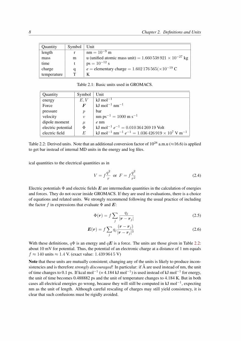
Quantity Symbol Unitlength r nm = 10−9 mmass m u (unified atomic mass unit) = 1.660 538 921× 10−27 kgtime t ps = 10−12 scharge q e = elementary charge = 1.602 176 565(×10−19 Ctemperature T K
Table 2.1: Basic units used in GROMACS.
Quantity Symbol Unitenergy E, V kJ mol−1
Force F kJ mol−1 nm−1
pressure p barvelocity v nm ps−1 = 1000 m s−1
dipole moment µ e nmelectric potential Φ kJ mol−1 e−1 = 0.010 364 269 19 Voltelectric field E kJ mol−1 nm−1 e−1 = 1.036 426 919× 107 V m−1
Table 2.2: Derived units. Note that an additional conversion factor of 1028 a.m.u (≈16.6) is appliedto get bar instead of internal MD units in the energy and log files.
ical quantities to the electrical quantities as in
V = fq2
ror F = f
q2
r2(2.4)
Electric potentials Φ and electric fieldsE are intermediate quantities in the calculation of energiesand forces. They do not occur inside GROMACS. If they are used in evaluations, there is a choiceof equations and related units. We strongly recommend following the usual practice of includingthe factor f in expressions that evaluate Φ and E:
Φ(r) = f∑j
qj|r − rj |
(2.5)
E(r) = f∑j
qj(r − rj)|r − rj |3
(2.6)
With these definitions, qΦ is an energy and qE is a force. The units are those given in Table 2.2:about 10 mV for potential. Thus, the potential of an electronic charge at a distance of 1 nm equalsf ≈ 140 units ≈ 1.4 V. (exact value: 1.439 964 5 V)
Note that these units are mutually consistent; changing any of the units is likely to produce incon-sistencies and is therefore strongly discouraged! In particular: if Å are used instead of nm, the unitof time changes to 0.1 ps. If kcal mol−1 (= 4.184 kJ mol−1) is used instead of kJ mol−1 for energy,the unit of time becomes 0.488882 ps and the unit of temperature changes to 4.184 K. But in bothcases all electrical energies go wrong, because they will still be computed in kJ mol−1, expectingnm as the unit of length. Although careful rescaling of charges may still yield consistency, it isclear that such confusions must be rigidly avoided.
2.3. Reduced units 9
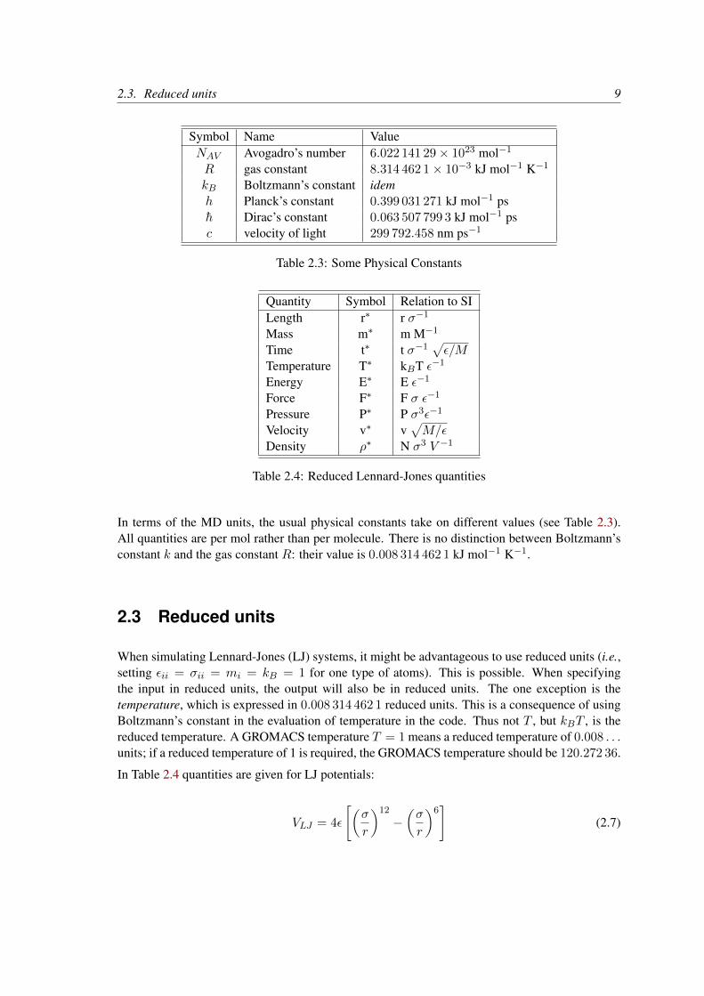
Symbol Name ValueNAV Avogadro’s number 6.022 141 29× 1023 mol−1
R gas constant 8.314 462 1× 10⁻³ kJ mol−1 K−1
kB Boltzmann’s constant idemh Planck’s constant 0.399 031 271 kJ mol−1 psh Dirac’s constant 0.063 507 799 3 kJ mol−1 psc velocity of light 299 792.458 nm ps−1
Table 2.3: Some Physical Constants
Quantity Symbol Relation to SILength r∗ r σ−1
Mass m∗ m M−1
Time t∗ t σ−1√ε/M
Temperature T∗ kBT ε−1
Energy E∗ E ε−1
Force F∗ F σ ε−1
Pressure P∗ P σ3ε−1
Velocity v∗ v√M/ε
Density ρ∗ N σ3 V −1
Table 2.4: Reduced Lennard-Jones quantities
In terms of the MD units, the usual physical constants take on different values (see Table 2.3).All quantities are per mol rather than per molecule. There is no distinction between Boltzmann’sconstant k and the gas constant R: their value is 0.008 314 462 1 kJ mol−1 K−1.
2.3 Reduced units
When simulating Lennard-Jones (LJ) systems, it might be advantageous to use reduced units (i.e.,setting εii = σii = mi = kB = 1 for one type of atoms). This is possible. When specifyingthe input in reduced units, the output will also be in reduced units. The one exception is thetemperature, which is expressed in 0.008 314 462 1 reduced units. This is a consequence of usingBoltzmann’s constant in the evaluation of temperature in the code. Thus not T , but kBT , is thereduced temperature. A GROMACS temperature T = 1 means a reduced temperature of 0.008 . . .units; if a reduced temperature of 1 is required, the GROMACS temperature should be 120.272 36.
In Table 2.4 quantities are given for LJ potentials:
VLJ = 4ε
[(σ
r
)12
−(σ
r
)6]
(2.7)

10 Chapter 2. Definitions and Units
2.4 Mixed or Double precision
GROMACS can be compiled in either mixed or double precision. Documentation of previousGROMACS versions referred to “single precision”, but the implementation has made selectiveuse of double precision for many years. Using single precision for all variables would lead to asignificant reduction in accuracy. Although in “mixed precision” all state vectors, i.e. particlecoordinates, velocities and forces, are stored in single precision, critical variables are double pre-cision. A typical example of the latter is the virial, which is a sum over all forces in the system,which have varying signs. In addition, in many parts of the code we managed to avoid double pre-cision for arithmetic, by paying attention to summation order or reorganization of mathematicalexpressions. The default configuration uses mixed precision, but it is easy to turn on double preci-sion by adding the option -DGMX_DOUBLE=on to cmake. Double precision will be 20 to 100%slower than mixed precision depending on the architecture you are running on. Double precisionwill use somewhat more memory and run input, energy and full-precision trajectory files will bealmost twice as large.
The energies in mixed precision are accurate up to the last decimal, the last one or two decimalsof the forces are non-significant. The virial is less accurate than the forces, since the virial is onlyone order of magnitude larger than the size of each element in the sum over all atoms (sec. A.1).In most cases this is not really a problem, since the fluctuations in the virial can be two ordersof magnitude larger than the average. Using cut-offs for the Coulomb interactions cause largeerrors in the energies, forces, and virial. Even when using a reaction-field or lattice sum method,the errors are larger than, or comparable to, the errors due to the partial use of single precision.Since MD is chaotic, trajectories with very similar starting conditions will diverge rapidly, thedivergence is faster in mixed precision than in double precision.
For most simulations, mixed precision is accurate enough. In some cases double precision isrequired to get reasonable results:
• normal mode analysis, for the conjugate gradient or l-bfgs minimization and the calculationand diagonalization of the Hessian
• long-term energy conservation, especially for large systems

Chapter 3
Algorithms
3.1 Introduction
In this chapter we first give describe some general concepts used in GROMACS: periodic bound-ary conditions (sec. 3.2) and the group concept (sec. 3.3). The MD algorithm is described insec. 3.4: first a global form of the algorithm is given, which is refined in subsequent subsections.The (simple) EM (Energy Minimization) algorithm is described in sec. 3.10. Some other algo-rithms for special purpose dynamics are described after this.
A few issues are of general interest. In all cases the system must be defined, consisting ofmolecules. Molecules again consist of particles with defined interaction functions. The detaileddescription of the topology of the molecules and of the force field and the calculation of forces isgiven in chapter 4. In the present chapter we describe other aspects of the algorithm, such as pairlist generation, update of velocities and positions, coupling to external temperature and pressure,conservation of constraints. The analysis of the data generated by an MD simulation is treated inchapter 8.
3.2 Periodic boundary conditions
The classical way to minimize edge effects in a finite system is to apply periodic boundary condi-tions. The atoms of the system to be simulated are put into a space-filling box, which is surroundedby translated copies of itself (Fig. 3.1). Thus there are no boundaries of the system; the artifactcaused by unwanted boundaries in an isolated cluster is now replaced by the artifact of periodicconditions. If the system is crystalline, such boundary conditions are desired (although motionsare naturally restricted to periodic motions with wavelengths fitting into the box). If one wishes tosimulate non-periodic systems, such as liquids or solutions, the periodicity by itself causes errors.The errors can be evaluated by comparing various system sizes; they are expected to be less severethan the errors resulting from an unnatural boundary with vacuum.
There are several possible shapes for space-filling unit cells. Some, like the rhombic dodecahedronand the truncated octahedron [20] are closer to being a sphere than a cube is, and are therefore

12 Chapter 3. Algorithms
j’ j’
i’ i’i’
i’
j’
i’ i’
y
x
y
x
j’ j’
i’
i’
i’i
j’
j’ j’j’
i’ii’
j’j’
j’
j
i’ i’i’
j’
i’ i’
j’
j’j’
j
Figure 3.1: Periodic boundary conditions in two dimensions.
better suited to the study of an approximately spherical macromolecule in solution, since fewersolvent molecules are required to fill the box given a minimum distance between macromolecularimages. At the same time, rhombic dodecahedra and truncated octahedra are special cases oftriclinic unit cells; the most general space-filling unit cells that comprise all possible space-fillingshapes [21]. For this reason, GROMACS is based on the triclinic unit cell.
GROMACS uses periodic boundary conditions, combined with the minimum image convention:only one – the nearest – image of each particle is considered for short-range non-bonded in-teraction terms. For long-range electrostatic interactions this is not always accurate enough, andGROMACS therefore also incorporates lattice sum methods such as Ewald Sum, PME and PPPM.
GROMACS supports triclinic boxes of any shape. The simulation box (unit cell) is defined by the3 box vectors a,b and c. The box vectors must satisfy the following conditions:
ay = az = bz = 0 (3.1)
ax > 0, by > 0, cz > 0 (3.2)
|bx| ≤1
2ax, |cx| ≤
1
2ax, |cy| ≤
1
2by (3.3)
Equations 3.1 can always be satisfied by rotating the box. Inequalities (3.2) and (3.3) can alwaysbe satisfied by adding and subtracting box vectors.
Even when simulating using a triclinic box, GROMACS always keeps the particles in a brick-shaped volume for efficiency, as illustrated in Fig. 3.1 for a 2-dimensional system. Therefore,from the output trajectory it might seem that the simulation was done in a rectangular box. Theprogram trjconv can be used to convert the trajectory to a different unit-cell representation.

3.2. Periodic boundary conditions 13
Figure 3.2: A rhombic dodecahedron and truncated octahedron (arbitrary orientations).
box type image box box vectors box vector anglesdistance volume a b c 6 bc 6 ac 6 ab
d 0 0cubic d d3 0 d 0 90 90 90
0 0 d
rhombic d 0 12 d
dodecahedron d 12
√2 d3 0 d 1
2 d 60 60 90
(xy-square) 0.707 d3 0 0 12
√2 d
rhombic d 12 d
12 d
dodecahedron d 12
√2 d3 0 1
2
√3 d 1
6
√3 d 60 60 60
(xy-hexagon) 0.707 d3 0 0 13
√6 d
truncated d 13 d −1
3 d
octahedron d 49
√3 d3 0 2
3
√2 d 1
3
√2 d 71.53 109.47 71.53
0.770 d3 0 0 13
√6 d
Table 3.1: The cubic box, the rhombic dodecahedron and the truncated octahedron.
It is also possible to simulate without periodic boundary conditions, but it is usually more efficientto simulate an isolated cluster of molecules in a large periodic box, since fast grid searching canonly be used in a periodic system.
3.2.1 Some useful box types
The three most useful box types for simulations of solvated systems are described in Table 3.1.The rhombic dodecahedron (Fig. 3.2) is the smallest and most regular space-filling unit cell. Eachof the 12 image cells is at the same distance. The volume is 71% of the volume of a cube havingthe same image distance. This saves about 29% of CPU-time when simulating a spherical orflexible molecule in solvent. There are two different orientations of a rhombic dodecahedron thatsatisfy equations 3.1, 3.2 and 3.3. The program editconf produces the orientation which hasa square intersection with the xy-plane. This orientation was chosen because the first two boxvectors coincide with the x and y-axis, which is easier to comprehend. The other orientation can

14 Chapter 3. Algorithms
be useful for simulations of membrane proteins. In this case the cross-section with the xy-plane isa hexagon, which has an area which is 14% smaller than the area of a square with the same imagedistance. The height of the box (cz) should be changed to obtain an optimal spacing. This boxshape not only saves CPU time, it also results in a more uniform arrangement of the proteins.
3.2.2 Cut-off restrictions
The minimum image convention implies that the cut-off radius used to truncate non-bonded inter-actions may not exceed half the shortest box vector:
Rc <1
2min(‖a‖, ‖b‖, ‖c‖), (3.4)
because otherwise more than one image would be within the cut-off distance of the force. When amacromolecule, such as a protein, is studied in solution, this restriction alone is not sufficient: inprinciple, a single solvent molecule should not be able to ‘see’ both sides of the macromolecule.This means that the length of each box vector must exceed the length of the macromolecule in thedirection of that edge plus two times the cut-off radius Rc. It is, however, common to compromisein this respect, and make the solvent layer somewhat smaller in order to reduce the computationalcost. For efficiency reasons the cut-off with triclinic boxes is more restricted. For grid search theextra restriction is weak:
Rc < min(ax, by, cz) (3.5)
For simple search the extra restriction is stronger:
Rc <1
2min(ax, by, cz) (3.6)
Each unit cell (cubic, rectangular or triclinic) is surrounded by 26 translated images. A particularimage can therefore always be identified by an index pointing to one of 27 translation vectors andconstructed by applying a translation with the indexed vector (see 3.4.3). Restriction (3.5) ensuresthat only 26 images need to be considered.
3.3 The group concept
The GROMACS MD and analysis programs use user-defined groups of atoms to perform certainactions on. The maximum number of groups is 256, but each atom can only belong to six differentgroups, one each of the following:
temperature-coupling group The temperature coupling parameters (reference temperature, timeconstant, number of degrees of freedom, see 3.4.4) can be defined for each T-coupling groupseparately. For example, in a solvated macromolecule the solvent (that tends to generatemore heating by force and integration errors) can be coupled with a shorter time constant toa bath than is a macromolecule, or a surface can be kept cooler than an adsorbing molecule.Many different T-coupling groups may be defined. See also center of mass groups below.
3.4. Molecular Dynamics 15
freeze group Atoms that belong to a freeze group are kept stationary in the dynamics. This isuseful during equilibration, e.g. to avoid badly placed solvent molecules giving unreasonablekicks to protein atoms, although the same effect can also be obtained by putting a restrainingpotential on the atoms that must be protected. The freeze option can be used, if desired, onjust one or two coordinates of an atom, thereby freezing the atoms in a plane or on a line.When an atom is partially frozen, constraints will still be able to move it, even in a frozendirection. A fully frozen atom can not be moved by constraints. Many freeze groups canbe defined. Frozen coordinates are unaffected by pressure scaling; in some cases this canproduce unwanted results, particularly when constraints are also used (in this case you willget very large pressures). Accordingly, it is recommended to avoid combining freeze groupswith constraints and pressure coupling. For the sake of equilibration it could suffice tostart with freezing in a constant volume simulation, and afterward use position restraints inconjunction with constant pressure.
accelerate group On each atom in an “accelerate group” an acceleration ag is imposed. Thisis equivalent to an external force. This feature makes it possible to drive the system intoa non-equilibrium state and enables the performance of non-equilibrium MD and hence toobtain transport properties.
energy-monitor group Mutual interactions between all energy-monitor groups are compiled dur-ing the simulation. This is done separately for Lennard-Jones and Coulomb terms. In prin-ciple up to 256 groups could be defined, but that would lead to 256×256 items! Better usethis concept sparingly.
All non-bonded interactions between pairs of energy-monitor groups can be excluded (seedetails in the User Guide). Pairs of particles from excluded pairs of energy-monitor groupsare not put into the pair list. This can result in a significant speedup for simulations whereinteractions within or between parts of the system are not required.
center of mass group In GROMACS the center of mass (COM) motion can be removed, foreither the complete system or for groups of atoms. The latter is useful, e.g. for systemswhere there is limited friction (e.g. gas systems) to prevent center of mass motion to occur.It makes sense to use the same groups for temperature coupling and center of mass motionremoval.
Compressed position output group In order to further reduce the size of the compressed tra-jectory file (.xtc or .tng), it is possible to store only a subset of all particles. All x-compression groups that are specified are saved, the rest are not. If no such groups arespecified, than all atoms are saved to the compressed trajectory file.
The use of groups in GROMACS tools is described in sec. 8.1.
3.4 Molecular Dynamics
A global flow scheme for MD is given in Fig. 3.3. Each MD or EM run requires as input a set ofinitial coordinates and – optionally – initial velocities of all particles involved. This chapter doesnot describe how these are obtained; for the setup of an actual MD run check the online manual atwww.gromacs.org.

16 Chapter 3. Algorithms
THE GLOBAL MD ALGORITHM
1. Input initial conditions
Potential interaction V as a function of atom positionsPositions r of all atoms in the systemVelocities v of all atoms in the system
⇓
repeat 2,3,4 for the required number of steps:
2. Compute forces
The force on any atom
F i = −∂V∂ri
is computed by calculating the force between non-bonded atompairs:
F i =∑j F ij
plus the forces due to bonded interactions (which may depend on 1,2, 3, or 4 atoms), plus restraining and/or external forces.
The potential and kinetic energies and the pressure tensor may becomputed.⇓
3. Update configuration
The movement of the atoms is simulated by numerically solvingNewton’s equations of motion
d2ridt2
=F i
miordridt
= vi;dvidt
=F i
mi
⇓4. if required: Output step
write positions, velocities, energies, temperature, pressure, etc.
Figure 3.3: The global MD algorithm

3.4. Molecular Dynamics 17
Velocity
Figure 3.4: A Maxwell-Boltzmann velocity distribution, generated from random numbers.
3.4.1 Initial conditions
Topology and force field
The system topology, including a description of the force field, must be read in. Force fields andtopologies are described in chapter 4 and 5, respectively. All this information is static; it is nevermodified during the run.
Coordinates and velocities
Then, before a run starts, the box size and the coordinates and velocities of all particles are re-quired. The box size and shape is determined by three vectors (nine numbers) b1, b2, b3, whichrepresent the three basis vectors of the periodic box.
If the run starts at t = t0, the coordinates at t = t0 must be known. The leap-frog algorithm, thedefault algorithm used to update the time step with ∆t (see 3.4.4), also requires that the velocitiesat t = t0− 1
2∆t are known. If velocities are not available, the program can generate initial atomicvelocities vi, i = 1 . . . 3N with a (Fig. 3.4) at a given absolute temperature T :
p(vi) =
√mi
2πkTexp
(−miv
2i
2kT
)(3.7)

18 Chapter 3. Algorithms
where k is Boltzmann’s constant (see chapter 2). To accomplish this, normally distributed randomnumbers are generated by adding twelve random numbers Rk in the range 0 ≤ Rk < 1 andsubtracting 6.0 from their sum. The result is then multiplied by the standard deviation of thevelocity distribution
√kT/mi. Since the resulting total energy will not correspond exactly to the
required temperature T , a correction is made: first the center-of-mass motion is removed and thenall velocities are scaled so that the total energy corresponds exactly to T (see eqn. 3.18).
Center-of-mass motion
The center-of-mass velocity is normally set to zero at every step; there is (usually) no net externalforce acting on the system and the center-of-mass velocity should remain constant. In practice,however, the update algorithm introduces a very slow change in the center-of-mass velocity, andtherefore in the total kinetic energy of the system – especially when temperature coupling is used.If such changes are not quenched, an appreciable center-of-mass motion can develop in long runs,and the temperature will be significantly misinterpreted. Something similar may happen due tooverall rotational motion, but only when an isolated cluster is simulated. In periodic systems withfilled boxes, the overall rotational motion is coupled to other degrees of freedom and does notcause such problems.
3.4.2 Neighbor searching
As mentioned in chapter 4, internal forces are either generated from fixed (static) lists, or fromdynamic lists. The latter consist of non-bonded interactions between any pair of particles. Whencalculating the non-bonded forces, it is convenient to have all particles in a rectangular box. Asshown in Fig. 3.1, it is possible to transform a triclinic box into a rectangular box. The outputcoordinates are always in a rectangular box, even when a dodecahedron or triclinic box was usedfor the simulation. Equation 3.1 ensures that we can reset particles in a rectangular box by firstshifting them with box vector c, then with b and finally with a. Equations 3.3, 3.4 and 3.5 ensurethat we can find the 14 nearest triclinic images within a linear combination that does not involvemultiples of box vectors.
Pair lists generation
The non-bonded pair forces need to be calculated only for those pairs i, j for which the distancerij between i and the nearest image of j is less than a given cut-off radiusRc. Some of the particlepairs that fulfill this criterion are excluded, when their interaction is already fully accounted for bybonded interactions. GROMACS employs a pair list that contains those particle pairs for whichnon-bonded forces must be calculated. The pair list contains particles i, a displacement vector forparticle i, and all particles j that are within rlist of this particular image of particle i. The listis updated every nstlist steps.
To make the neighbor list, all particles that are close (i.e. within the neighbor list cut-off) to a givenparticle must be found. This searching, usually called neighbor search (NS) or pair search, involvesperiodic boundary conditions and determining the image (see sec. 3.2). The search algorithm isO(N), although a simpler O(N2) algorithm is still available under some conditions.

3.4. Molecular Dynamics 19
Cut-off schemes: group versus Verlet
From version 4.6, GROMACS supports two different cut-off scheme setups: the original onebased on particle groups and one using a Verlet buffer. There are some important differencesthat affect results, performance and feature support. The group scheme can be made to work(almost) like the Verlet scheme, but this will lead to a decrease in performance. The group schemeis especially fast for water molecules, which are abundant in many simulations, but on the mostrecent x86 processors, this advantage is negated by the better instruction-level parallelism availablein the Verlet-scheme implementation. The group scheme is deprecated in version 5.0, and will beremoved in a future version. For practical details of choosing and setting up cut-off schemes,please see the User Guide.
In the group scheme, a neighbor list is generated consisting of pairs of groups of at least oneparticle. These groups were originally charge groups (see sec. 3.4.2), but with a proper treatmentof long-range electrostatics, performance in unbuffered simulations is their only advantage. Apair of groups is put into the neighbor list when their center of geometry is within the cut-offdistance. Interactions between all particle pairs (one from each charge group) are calculated fora certain number of MD steps, until the neighbor list is updated. This setup is efficient, as theneighbor search only checks distance between charge-group pair, not particle pairs (saves a factorof 3×3 = 9 with a three-particle water model) and the non-bonded force kernels can be optimizedfor, say, a water molecule “group”. Without explicit buffering, this setup leads to energy drift assome particle pairs which are within the cut-off don’t interact and some outside the cut-off dointeract. This can be caused by
• particles moving across the cut-off between neighbor search steps, and/or
• for charge groups consisting of more than one particle, particle pairs moving in/out of thecut-off when their charge group center of geometry distance is outside/inside of the cut-off.
Explicitly adding a buffer to the neighbor list will remove such artifacts, but this comes at a highcomputational cost. How severe the artifacts are depends on the system, the properties in whichyou are interested, and the cut-off setup.
The Verlet cut-off scheme uses a buffered pair list by default. It also uses clusters of particles, butthese are not static as in the group scheme. Rather, the clusters are defined spatially and consistof 4 or 8 particles, which is convenient for stream computing, using e.g. SSE, AVX or CUDA onGPUs. At neighbor search steps, a pair list is created with a Verlet buffer, ie. the pair-list cut-offis larger than the interaction cut-off. In the non-bonded kernels, interactions are only computedwhen a particle pair is within the cut-off distance at that particular time step. This ensures thatas particles move between pair search steps, forces between nearly all particles within the cut-offdistance are calculated. We say nearly all particles, because GROMACS uses a fixed pair listupdate frequency for efficiency. A particle-pair, whose distance was outside the cut-off, couldpossibly move enough during this fixed number of steps that its distance is now within the cut-off. This small chance results in a small energy drift, and the size of the chance depends on thetemperature. When temperature coupling is used, the buffer size can be determined automatically,given a certain tolerance on the energy drift.
The Verlet cut-off scheme is implemented in a very efficient fashion based on clusters of particles.The simplest example is a cluster size of 4 particles. The pair list is then constructed based on

20 Chapter 3. Algorithms
cluster pairs. The cluster-pair search is much faster searching based on particle pairs, because4 × 4 = 16 particle pairs are put in the list at once. The non-bonded force calculation kernel canthen calculate many particle-pair interactions at once, which maps nicely to SIMD or SIMT unitson modern hardware, which can perform multiple floating operations at once. These non-bondedkernels are much faster than the kernels used in the group scheme for most types of systems,particularly on newer hardware.
Additionally, when the list buffer is determined automatically as described below, we also applydynamic pair list pruning. The pair list can be constructed infrequently, but that can lead to a lotof pairs in the list that are outside the cut-off range for all or most of the life time of this pairlist. Such pairs can be pruned out by applying a cluster-pair kernel that only determines whichclusters are in range. Because of the way the non-bonded data is regularized in GROMACS, thiskernel is an order of magnitude faster than the search and the interaction kernel. On the GPU thispruning is overlapped with the integration on the CPU, so it is free in most cases. Therefore wecan prune every 4-10 integration steps with little overhead and significantly reduce the number ofcluster pairs in the interaction kernel. This procedure is applied automatically, unless the user setthe pair-list buffer size manually.
Energy drift and pair-list buffering
For a canonical (NVT) ensemble, the average energy error caused by diffusion of j particles fromoutside the pair-list cut-off r` to inside the interaction cut-off rc over the lifetime of the list canbe determined from the atomic displacements and the shape of the potential at the cut-off. Thedisplacement distribution along one dimension for a freely moving particle with massm over timet at temperature T is a GaussianG(x) of zero mean and variance σ2 = t2kBT/m. For the distancebetween two particles, the variance changes to σ2 = σ2
12 = t2kBT (1/m1 + 1/m2). Note thatin practice particles usually interact with (bump into) other particles over time t and therefore thereal displacement distribution is much narrower. Given a non-bonded interaction cut-off distanceof rc and a pair-list cut-off r` = rc + rb for rb the Verlet buffer size, we can then write the averageenergy error after time t for all missing pair interactions between a single i particle of type 1surrounded by all j particles that are of type 2 with number density ρ2, when the inter-particledistance changes from r0 to rt, as:
〈∆V 〉 =
∫ rc
0
∫ ∞r`
4πr20ρ2V (rt)G
(rt − r0
σ
)dr0 drt (3.8)
To evaluate this analytically, we need to make some approximations. First we replace V (rt) bya Taylor expansion around rc, then we can move the lower bound of the integral over r0 to −∞which will simplify the result:
〈∆V 〉 ≈∫ rc
−∞
∫ ∞r`
4πr20ρ2
[V ′(rc)(rt − rc) +
V ′′(rc)1
2(rt − rc)2 +
V ′′′(rc)1
6(rt − rc)3 +
O((rt − rc)4
) ]G
(rt − r0
σ
)dr0 drt (3.9)

3.4. Molecular Dynamics 21
Replacing the factor r20 by (r` + σ)2, which results in a slight overestimate, allows us to calculate
the integrals analytically:
〈∆V 〉 ≈ 4π(r` + σ)2ρ2
∫ rc
−∞
∫ ∞r`
[V ′(rc)(rt − rc) +
V ′′(rc)1
2(rt − rc)2 +
V ′′′(rc)1
6(rt − rc)3
]G
(rt − r0
σ
)dr0 drt (3.10)
= 4π(r` + σ)2ρ2
1
2V ′(rc)
[rbσG
(rbσ
)− (r2
b + σ2)E
(rbσ
)]+
1
6V ′′(rc)
[σ(r2
b + 2σ2)G
(rbσ
)− rb(r2
b + 3σ2)E
(rbσ
)]+
1
24V ′′′(rc)
[rbσ(r2
b + 5σ2)G
(rbσ
)− (r4
b + 6r2bσ
2 + 3σ4)E
(rbσ
)](3.11)
where G(x) is a Gaussian distribution with 0 mean and unit variance and E(x) = 12erfc(x/
√2).
We always want to achieve small energy error, so σ will be small compared to both rc and r`,thus the approximations in the equations above are good, since the Gaussian distribution decaysrapidly. The energy error needs to be averaged over all particle pair types and weighted withthe particle counts. In GROMACS we don’t allow cancellation of error between pair types, sowe average the absolute values. To obtain the average energy error per unit time, it needs to bedivided by the neighbor-list life time t = (nstlist − 1) × dt. The function can not be invertedanalytically, so we use bisection to obtain the buffer size rb for a target drift. Again we note that inpractice the error we usually be much smaller than this estimate, as in the condensed phase particledisplacements will be much smaller than for freely moving particles, which is the assumption usedhere.
When (bond) constraints are present, some particles will have fewer degrees of freedom. This willreduce the energy errors. For simplicity, we only consider one constraint per particle, the heaviestparticle in case a particle is involved in multiple constraints. This simplification overestimates thedisplacement. The motion of a constrained particle is a superposition of the 3D motion of thecenter of mass of both particles and a 2D rotation around the center of mass. The displacement inan arbitrary direction of a particle with 2 degrees of freedom is not Gaussian, but rather followsthe complementary error function:
√π
2√
2σerfc
( |r|√2σ
)(3.12)
where σ2 is again t2kBT/m. This distribution can no longer be integrated analytically to obtainthe energy error. But we can generate a tight upper bound using a scaled and shifted Gaussiandistribution (not shown). This Gaussian distribution can then be used to calculate the energy erroras described above. The rotation displacement around the center of mass can not be more than thelength of the arm. To take this into account, we scale σ in eqn. 3.12 (details not presented here) toobtain an overestimate of the real displacement. This latter effect significantly reduces the buffer

22 Chapter 3. Algorithms
0 0.02 0.04 0.06 0.08 0.1
Verlet buffer (nm)
10−6
10−5
10−4
10−3
10−2
drift
pe
r a
tom
(kJ/m
ol/p
s)
estimate 1x1
estimate 4x4
double precision
mixed precision
Figure 3.5: Energy drift per atom for an SPC/E water system at 300K with a time step of 2 fs anda pair-list update period of 10 steps (pair-list life time: 18 fs). PME was used with ewald-rtolset to 10−5; this parameter affects the shape of the potential at the cut-off. Error estimates due tofinite Verlet buffer size are shown for a 1 × 1 atom pair list and 4 × 4 atom pair list without andwith (dashed line) cancellation of positive and negative errors. Real energy drift is shown for sim-ulations using double- and mixed-precision settings. Rounding errors in the SETTLE constraintalgorithm from the use of single precision causes the drift to become negative at large buffer size.Note that at zero buffer size, the real drift is small because positive (H-H) and negative (O-H)energy errors cancel.
size for longer neighborlist lifetimes in e.g. water, as constrained hydrogens are by far the fastestparticles, but they can not move further than 0.1 nm from the heavy atom they are connected to.
There is one important implementation detail that reduces the energy errors caused by the finiteVerlet buffer list size. The derivation above assumes a particle pair-list. However, the GROMACSimplementation uses a cluster pair-list for efficiency. The pair list consists of pairs of clusters of4 particles in most cases, also called a 4 × 4 list, but the list can also be 4 × 8 (GPU CUDAkernels and AVX 256-bit single precision kernels) or 4 × 2 (SSE double-precision kernels). Thismeans that the pair-list is effectively much larger than the corresponding 1 × 1 list. Thus slightlybeyond the pair-list cut-off there will still be a large fraction of particle pairs present in the list.This fraction can be determined in a simulation and accurately estimated under some reasonableassumptions. The fraction decreases with increasing pair-list range, meaning that a smaller buffercan be used. For typical all-atom simulations with a cut-off of 0.9 nm this fraction is around 0.9,which gives a reduction in the energy errors of a factor of 10. This reduction is taken into accountduring the automatic Verlet buffer calculation and results in a smaller buffer size.
In Fig. 3.5 one can see that for small buffer sizes the drift of the total energy is much smallerthan the pair energy error tolerance, due to cancellation of errors. For larger buffer size, the errorestimate is a factor of 6 higher than drift of the total energy, or alternatively the buffer estimate is0.024 nm too large. This is because the protons don’t move freely over 18 fs, but rather vibrate.

3.4. Molecular Dynamics 23
j
i
i’
Figure 3.6: Grid search in two dimensions. The arrows are the box vectors.
Cut-off artifacts and switched interactions
With the Verlet scheme, the pair potentials are shifted to be zero at the cut-off, which makes thepotential the integral of the force. This is only possible in the group scheme if the shape of thepotential is such that its value is zero at the cut-off distance. However, there can still be energydrift when the forces are non-zero at the cut-off. This effect is extremely small and often notnoticeable, as other integration errors (e.g. from constraints) may dominate. To completely avoidcut-off artifacts, the non-bonded forces can be switched exactly to zero at some distance smallerthan the neighbor list cut-off (there are several ways to do this in GROMACS, see sec. 4.1.5). Onethen has a buffer with the size equal to the neighbor list cut-off less the longest interaction cut-off.
Simple search
Due to eqns. 3.1 and 3.6, the vector rij connecting images within the cut-off Rc can be found byconstructing:
r′′′ = rj − ri (3.13)
r′′ = r′′′ − c ∗ round(r′′′z /cz) (3.14)
r′ = r′′ − b ∗ round(r′′y/by) (3.15)
rij = r′ − a ∗ round(r′x/ax) (3.16)
When distances between two particles in a triclinic box are needed that do not obey eqn. 3.1, manyshifts of combinations of box vectors need to be considered to find the nearest image.
Grid search
The grid search is schematically depicted in Fig. 3.6. All particles are put on the NS grid, with thesmallest spacing ≥ Rc/2 in each of the directions. In the direction of each box vector, a particle

24 Chapter 3. Algorithms
i has three images. For each direction the image may be -1,0 or 1, corresponding to a translationover -1, 0 or +1 box vector. We do not search the surrounding NS grid cells for neighbors ofi and then calculate the image, but rather construct the images first and then search neighborscorresponding to that image of i. As Fig. 3.6 shows, some grid cells may be searched more thanonce for different images of i. This is not a problem, since, due to the minimum image convention,at most one image will “see” the j-particle. For every particle, fewer than 125 (53) neighboringcells are searched. Therefore, the algorithm scales linearly with the number of particles. Althoughthe prefactor is large, the scaling behavior makes the algorithm far superior over the standardO(N2) algorithm when there are more than a few hundred particles. The grid search is equallyfast for rectangular and triclinic boxes. Thus for most protein and peptide simulations the rhombicdodecahedron will be the preferred box shape.
Charge groups
Charge groups were originally introduced to reduce cut-off artifacts of Coulomb interactions.When a plain cut-off is used, significant jumps in the potential and forces arise when atoms with(partial) charges move in and out of the cut-off radius. When all chemical moieties have a netcharge of zero, these jumps can be reduced by moving groups of atoms with net charge zero,called charge groups, in and out of the neighbor list. This reduces the cut-off effects from thecharge-charge level to the dipole-dipole level, which decay much faster. With the advent of fullrange electrostatics methods, such as particle-mesh Ewald (sec. 4.8.2), the use of charge groupsis no longer required for accuracy. It might even have a slight negative effect on the accuracy orefficiency, depending on how the neighbor list is made and the interactions are calculated.
But there is still an important reason for using “charge groups”: efficiency with the group cut-offscheme. Where applicable, neighbor searching is carried out on the basis of charge groups whichare defined in the molecular topology. If the nearest image distance between the geometricalcenters of the atoms of two charge groups is less than the cut-off radius, all atom pairs betweenthe charge groups are included in the pair list. The neighbor searching for a water system, forinstance, is 32 = 9 times faster when each molecule is treated as a charge group. Also the highlyoptimized water force loops (see sec. A.2.1) only work when all atoms in a water molecule forma single charge group. Currently the name neighbor-search group would be more appropriate, butthe name charge group is retained for historical reasons. When developing a new force field, theadvice is to use charge groups of 3 to 4 atoms for optimal performance. For all-atom force fieldsthis is relatively easy, as one can simply put hydrogen atoms, and in some case oxygen atoms, inthe same charge group as the heavy atom they are connected to; for example: CH3, CH2, CH,NH2, NH, OH, CO2, CO.
With the Verlet cut-off scheme, charge groups are ignored.
3.4.3 Compute forces
Potential energy
When forces are computed, the potential energy of each interaction term is computed as well. Thetotal potential energy is summed for various contributions, such as Lennard-Jones, Coulomb, and

3.4. Molecular Dynamics 25
bonded terms. It is also possible to compute these contributions for energy-monitor groups ofatoms that are separately defined (see sec. 3.3).
Kinetic energy and temperature
The temperature is given by the total kinetic energy of the N -particle system:
Ekin =1
2
N∑i=1
miv2i (3.17)
From this the absolute temperature T can be computed using:
1
2NdfkT = Ekin (3.18)
where k is Boltzmann’s constant and Ndf is the number of degrees of freedom which can becomputed from:
Ndf = 3N −Nc −Ncom (3.19)
HereNc is the number of constraints imposed on the system. When performing molecular dynam-ics Ncom = 3 additional degrees of freedom must be removed, because the three center-of-massvelocities are constants of the motion, which are usually set to zero. When simulating in vacuo,the rotation around the center of mass can also be removed, in this case Ncom = 6. When morethan one temperature-coupling group is used, the number of degrees of freedom for group i is:
N idf = (3N i −N i
c)3N −Nc −Ncom
3N −Nc(3.20)
The kinetic energy can also be written as a tensor, which is necessary for pressure calculation in atriclinic system, or systems where shear forces are imposed:
Ekin =1
2
N∑i
mivi ⊗ vi (3.21)
Pressure and virial
The pressure tensor P is calculated from the difference between kinetic energy Ekin and the virialΞ:
P =2
V(Ekin −Ξ) (3.22)
where V is the volume of the computational box. The scalar pressure P , which can be used forpressure coupling in the case of isotropic systems, is computed as:
P = trace(P)/3 (3.23)
The virial Ξ tensor is defined as:
Ξ = −1
2
∑i<j
rij ⊗ F ij (3.24)
The GROMACS implementation of the virial computation is described in sec. A.1.

26 Chapter 3. Algorithms
1 20 t
x v x
Figure 3.7: The Leap-Frog integration method. The algorithm is called Leap-Frog because r andv are leaping like frogs over each other’s backs.
3.4.4 The leap-frog integrator
The default MD integrator in GROMACS is the so-called leap-frog algorithm [22] for the inte-gration of the equations of motion. When extremely accurate integration with temperature and/orpressure coupling is required, the velocity Verlet integrators are also present and may be preferable(see 3.4.5). The leap-frog algorithm uses positions r at time t and velocities v at time t− 1
2∆t; itupdates positions and velocities using the forces F (t) determined by the positions at time t usingthese relations:
v(t+1
2∆t) = v(t− 1
2∆t) +
∆t
mF (t) (3.25)
r(t+ ∆t) = r(t) + ∆tv(t+1
2∆t) (3.26)
The algorithm is visualized in Fig. 3.7. It produces trajectories that are identical to the Verlet [23]algorithm, whose position-update relation is
r(t+ ∆t) = 2r(t)− r(t−∆t) +1
mF (t)∆t2 +O(∆t4) (3.27)
The algorithm is of third order in r and is time-reversible. See ref. [24] for the merits of thisalgorithm and comparison with other time integration algorithms.
The equations of motion are modified for temperature coupling and pressure coupling, and ex-tended to include the conservation of constraints, all of which are described below.
3.4.5 The velocity Verlet integrator
The velocity Verlet algorithm [25] is also implemented in GROMACS, though it is not yet fullyintegrated with all sets of options. In velocity Verlet, positions r and velocities v at time t are usedto integrate the equations of motion; velocities at the previous half step are not required.
v(t+1
2∆t) = v(t) +
∆t
2mF (t) (3.28)
r(t+ ∆t) = r(t) + ∆tv(t+1
2∆t) (3.29)
v(t+ ∆t) = v(t+1
2∆t) +
∆t
2mF (t+ ∆t) (3.30)

3.4. Molecular Dynamics 27
or, equivalently,
r(t+ ∆t) = r(t) + ∆tv +∆t2
2mF (t) (3.31)
v(t+ ∆t) = v(t) +∆t
2m[F (t) + F (t+ ∆t)] (3.32)
With no temperature or pressure coupling, and with corresponding starting points, leap-frog andvelocity Verlet will generate identical trajectories, as can easily be verified by hand from the equa-tions above. Given a single starting file with the same starting point x(0) and v(0), leap-frogand velocity Verlet will not give identical trajectories, as leap-frog will interpret the velocities ascorresponding to t = −1
2∆t, while velocity Verlet will interpret them as corresponding to thetimepoint t = 0.
3.4.6 Understanding reversible integrators: The Trotter decomposition
To further understand the relationship between velocity Verlet and leap-frog integration, we intro-duce the reversible Trotter formulation of dynamics, which is also useful to understanding imple-mentations of thermostats and barostats in GROMACS.
A system of coupled, first-order differential equations can be evolved from time t = 0 to time t byapplying the evolution operator
Γ(t) = exp(iLt)Γ(0)
iL = Γ · ∇Γ, (3.33)
where L is the Liouville operator, and Γ is the multidimensional vector of independent variables(positions and velocities). A short-time approximation to the true operator, accurate at time ∆t =t/P , is applied P times in succession to evolve the system as
Γ(t) =P∏i=1
exp(iL∆t)Γ(0) (3.34)
For NVE dynamics, the Liouville operator is
iL =N∑i=1
vi · ∇ri +N∑i=1
1
miF (ri) · ∇vi . (3.35)
This can be split into two additive operators
iL1 =N∑i=1
1
miF (ri) · ∇vi
iL2 =N∑i=1
vi · ∇ri (3.36)
Then a short-time, symmetric, and thus reversible approximation of the true dynamics will be
exp(iL∆t) = exp(iL21
2∆t) exp(iL1∆t) exp(iL2
1
2∆t) +O(∆t3). (3.37)

28 Chapter 3. Algorithms
This corresponds to velocity Verlet integration. The first exponential term over 12∆t corresponds
to a velocity half-step, the second exponential term over ∆t corresponds to a full velocity step,and the last exponential term over 1
2∆t is the final velocity half step. For future times t = n∆t,this becomes
exp(iLn∆t) ≈(
exp(iL21
2∆t) exp(iL1∆t) exp(iL2
1
2∆t)
)n≈ exp(iL2
1
2∆t)
(exp(iL1∆t) exp(iL2∆t)
)n−1
exp(iL1∆t) exp(iL21
2∆t) (3.38)
This formalism allows us to easily see the difference between the different flavors of Verlet inte-grators. The leap-frog integrator can be seen as starting with Eq. 3.37 with the exp (iL1∆t) term,instead of the half-step velocity term, yielding
exp(iLn∆t) = exp (iL1∆t) exp (iL2∆t) +O(∆t3). (3.39)
Here, the full step in velocity is between t − 12∆t and t + 1
2∆t, since it is a combination of thevelocity half steps in velocity Verlet. For future times t = n∆t, this becomes
exp(iLn∆t) ≈(
exp (iL1∆t) exp (iL2∆t)
)n. (3.40)
Although at first this does not appear symmetric, as long as the full velocity step is between t− 12∆t
and t+ 12∆t, then this is simply a way of starting velocity Verlet at a different place in the cycle.
Even though the trajectory and thus potential energies are identical between leap-frog and velocityVerlet, the kinetic energy and temperature will not necessarily be the same. Standard velocityVerlet uses the velocities at the t to calculate the kinetic energy and thus the temperature only attime t; the kinetic energy is then a sum over all particles
KEfull(t) =∑i
(1
2mivi(t)
)2
=∑i
1
2mi
(1
2vi(t−
1
2∆t) +
1
2vi(t+
1
2∆t)
)2
, (3.41)
with the square on the outside of the average. Standard leap-frog calculates the kinetic energy attime t based on the average kinetic energies at the timesteps t+ 1
2∆t and t− 12∆t, or the sum over
all particles
KEaverage(t) =∑i
1
2mi
(1
2vi(t−
1
2∆t)2 +
1
2vi(t+
1
2∆t)2
), (3.42)
where the square is inside the average.
A non-standard variant of velocity Verlet which averages the kinetic energies KE(t + 12∆t) and
KE(t − 12∆t), exactly like leap-frog, is also now implemented in GROMACS (as .mdp file
option md-vv-avek). Without temperature and pressure coupling, velocity Verlet with half-step-averaged kinetic energies and leap-frog will be identical up to numerical precision. For
3.4. Molecular Dynamics 29
temperature- and pressure-control schemes, however, velocity Verlet with half-step-averaged ki-netic energies and leap-frog will be different, as will be discussed in the section in thermostats andbarostats.
The half-step-averaged kinetic energy and temperature are slightly more accurate for a given stepsize; the difference in average kinetic energies using the half-step-averaged kinetic energies (mdand md-vv-avek) will be closer to the kinetic energy obtained in the limit of small step size thanwill the full-step kinetic energy (using md-vv). For NVE simulations, this difference is usually notsignificant, since the positions and velocities of the particles are still identical; it makes a differencein the way the the temperature of the simulations are interpreted, but not in the trajectories thatare produced. Although the kinetic energy is more accurate with the half-step-averaged method,meaning that it changes less as the timestep gets large, it is also more noisy. The RMS deviationof the total energy of the system (sum of kinetic plus potential) in the half-step-averaged kineticenergy case will be higher (about twice as high in most cases) than the full-step kinetic energy.The drift will still be the same, however, as again, the trajectories are identical.
For NVT simulations, however, there will be a difference, as discussed in the section on temper-ature control, since the velocities of the particles are adjusted such that kinetic energies of thesimulations, which can be calculated either way, reach the distribution corresponding to the settemperature. In this case, the three methods will not give identical results.
Because the velocity and position are both defined at the same time t the velocity Verlet integratorcan be used for some methods, especially rigorously correct pressure control methods, that are notactually possible with leap-frog. The integration itself takes negligibly more time than leap-frog,but twice as many communication calls are currently required. In most cases, and especially forlarge systems where communication speed is important for parallelization and differences betweenthermodynamic ensembles vanish in the 1/N limit, and when only NVT ensembles are required,leap-frog will likely be the preferred integrator. For pressure control simulations where the finedetails of the thermodynamics are important, only velocity Verlet allows the true ensemble to becalculated. In either case, simulation with double precision may be required to get fine details ofthermodynamics correct.
3.4.7 Multiple time stepping
Several other simulation packages uses multiple time stepping for bonds and/or the PME meshforces. In GROMACS we have not implemented this (yet), since we use a different philosophy.Bonds can be constrained (which is also a more sound approximation of a physical quantumoscillator), which allows the smallest time step to be increased to the larger one. This not onlyhalves the number of force calculations, but also the update calculations. For even larger timesteps, angle vibrations involving hydrogen atoms can be removed using virtual interaction sites(see sec. 6.10), which brings the shortest time step up to PME mesh update frequency of a multipletime stepping scheme.
3.4.8 Temperature coupling
While direct use of molecular dynamics gives rise to the NVE (constant number, constant vol-ume, constant energy ensemble), most quantities that we wish to calculate are actually from a

30 Chapter 3. Algorithms
constant temperature (NVT) ensemble, also called the canonical ensemble. GROMACS can usethe weak-coupling scheme of Berendsen [26], stochastic randomization through the Andersenthermostat [27], the extended ensemble Nosé-Hoover scheme [28, 29], or a velocity-rescalingscheme [30] to simulate constant temperature, with advantages of each of the schemes laid outbelow.
There are several other reasons why it might be necessary to control the temperature of the system(drift during equilibration, drift as a result of force truncation and integration errors, heating due toexternal or frictional forces), but this is not entirely correct to do from a thermodynamic standpoint,and in some cases only masks the symptoms (increase in temperature of the system) rather than theunderlying problem (deviations from correct physics in the dynamics). For larger systems, errorsin ensemble averages and structural properties incurred by using temperature control to removeslow drifts in temperature appear to be negligible, but no completely comprehensive comparisonshave been carried out, and some caution must be taking in interpreting the results.
When using temperature and/or pressure coupling the total energy is no longer conserved. In-stead there is a conserved energy quantity the formula of which will depend on the combination ortemperature and pressure coupling algorithm used. For all coupling algorithms, except for Ander-sen temperature coupling and Parrinello-Rahman pressure coupling combined with shear stress,the conserved energy quantity is computed and stored in the energy and log file. Note that thisquantity will not be conserved when external forces are applied to the system, such as pulling ongroup with a changing distance or an electric field. Furthermore, how well the energy is conserveddepends on the accuracy of all algorithms involved in the simulation. Usually the algorithms thatcause most drift are constraints and the pair-list buffer, depending on the parameters used.
Berendsen temperature coupling
The Berendsen algorithm mimics weak coupling with first-order kinetics to an external heat bathwith given temperature T0. See ref. [31] for a comparison with the Nosé-Hoover scheme. Theeffect of this algorithm is that a deviation of the system temperature from T0 is slowly correctedaccording to:
dTdt
=T0 − Tτ
(3.43)
which means that a temperature deviation decays exponentially with a time constant τ . Thismethod of coupling has the advantage that the strength of the coupling can be varied and adaptedto the user requirement: for equilibration purposes the coupling time can be taken quite short (e.g.0.01 ps), but for reliable equilibrium runs it can be taken much longer (e.g. 0.5 ps) in which caseit hardly influences the conservative dynamics.
The Berendsen thermostat suppresses the fluctuations of the kinetic energy. This means that onedoes not generate a proper canonical ensemble, so rigorously, the sampling will be incorrect. Thiserror scales with 1/N , so for very large systems most ensemble averages will not be affected sig-nificantly, except for the distribution of the kinetic energy itself. However, fluctuation properties,such as the heat capacity, will be affected. A similar thermostat which does produce a correctensemble is the velocity rescaling thermostat [30] described below.
The heat flow into or out of the system is affected by scaling the velocities of each particle every

3.4. Molecular Dynamics 31
step, or every nTC steps, with a time-dependent factor λ, given by:
λ =
[1 +
nTC∆t
τT
T0
T (t− 12∆t)
− 1
]1/2
(3.44)
The parameter τT is close, but not exactly equal, to the time constant τ of the temperature coupling(eqn. 3.43):
τ = 2CV τT /Ndfk (3.45)
where CV is the total heat capacity of the system, k is Boltzmann’s constant, and Ndf is thetotal number of degrees of freedom. The reason that τ 6= τT is that the kinetic energy changecaused by scaling the velocities is partly redistributed between kinetic and potential energy andhence the change in temperature is less than the scaling energy. In practice, the ratio τ/τT rangesfrom 1 (gas) to 2 (harmonic solid) to 3 (water). When we use the term “temperature couplingtime constant,” we mean the parameter τT . Note that in practice the scaling factor λ is limitedto the range of 0.8 <= λ <= 1.25, to avoid scaling by very large numbers which may crash thesimulation. In normal use, λ will always be much closer to 1.0.
The thermostat modifies the kinetic energy at each scaling step by:
∆Ek = (λ− 1)2Ek (3.46)
The sum of these changes over the run needs to subtracted from the total energy to obtain theconserved energy quantity.
Velocity-rescaling temperature coupling
The velocity-rescaling thermostat [30] is essentially a Berendsen thermostat (see above) with anadditional stochastic term that ensures a correct kinetic energy distribution by modifying it accord-ing to
dK = (K0 −K)dtτT
+ 2
√KK0
Nf
dW√τT, (3.47)
where K is the kinetic energy, Nf the number of degrees of freedom and dW a Wiener process.There are no additional parameters, except for a random seed. This thermostat produces a correctcanonical ensemble and still has the advantage of the Berendsen thermostat: first order decay oftemperature deviations and no oscillations.
Andersen thermostat
One simple way to maintain a thermostatted ensemble is to take an NV E integrator and pe-riodically re-select the velocities of the particles from a Maxwell-Boltzmann distribution. [27]This can either be done by randomizing all the velocities simultaneously (massive collision) ev-ery τT /∆t steps (andersen-massive), or by randomizing every particle with some smallprobability every timestep (andersen), equal to ∆t/τ , where in both cases ∆t is the timestepand τT is a characteristic coupling time scale. Because of the way constraints operate, all par-ticles in the same constraint group must be randomized simultaneously. Because of paralleliza-tion issues, the andersen version cannot currently (5.0) be used in systems with constraints.

32 Chapter 3. Algorithms
andersen-massive can be used regardless of constraints. This thermostat is also currentlyonly possible with velocity Verlet algorithms, because it operates directly on the velocities at eachtimestep.
This algorithm completely avoids some of the ergodicity issues of other thermostatting algorithms,as energy cannot flow back and forth between energetically decoupled components of the systemas in velocity scaling motions. However, it can slow down the kinetics of system by randomizingcorrelated motions of the system, including slowing sampling when τT is at moderate levels (lessthan 10 ps). This algorithm should therefore generally not be used when examining kinetics ortransport properties of the system. [32]
Nosé-Hoover temperature coupling
The Berendsen weak-coupling algorithm is extremely efficient for relaxing a system to the targettemperature, but once the system has reached equilibrium it might be more important to probe acorrect canonical ensemble. This is unfortunately not the case for the weak-coupling scheme.
To enable canonical ensemble simulations, GROMACS also supports the extended-ensemble ap-proach first proposed by Nosé [28] and later modified by Hoover [29]. The system Hamiltonianis extended by introducing a thermal reservoir and a friction term in the equations of motion. Thefriction force is proportional to the product of each particle’s velocity and a friction parameter, ξ.This friction parameter (or “heat bath” variable) is a fully dynamic quantity with its own momen-tum (pξ) and equation of motion; the time derivative is calculated from the difference between thecurrent kinetic energy and the reference temperature.
In this formulation, the particles’ equations of motion in Fig. 3.3 are replaced by:
d2ridt2
=F i
mi− pξQ
dridt, (3.48)
where the equation of motion for the heat bath parameter ξ is:
dpξdt
= (T − T0) . (3.49)
The reference temperature is denoted T0, while T is the current instantaneous temperature of thesystem. The strength of the coupling is determined by the constant Q (usually called the “massparameter” of the reservoir) in combination with the reference temperature. 1
The conserved quantity for the Nosé-Hoover equations of motion is not the total energy, but rather
H =N∑i=1
pi2mi
+ U (r1, r2, . . . , rN ) +p2ξ
2Q+NfkTξ, (3.50)
where Nf is the total number of degrees of freedom.
In our opinion, the mass parameter is a somewhat awkward way of describing coupling strength,especially due to its dependence on reference temperature (and some implementations even in-clude the number of degrees of freedom in your system when defining Q). To maintain the cou-pling strength, one would have to change Q in proportion to the change in reference temperature.
1Note that some derivations, an alternative notation ξalt = vξ = pξ/Q is used.

3.4. Molecular Dynamics 33
For this reason, we prefer to let the GROMACS user work instead with the period τT of the oscil-lations of kinetic energy between the system and the reservoir instead. It is directly related to Qand T0 via:
Q =τ2TT0
4π2. (3.51)
This provides a much more intuitive way of selecting the Nosé-Hoover coupling strength (similarto the weak-coupling relaxation), and in addition τT is independent of system size and referencetemperature.
It is however important to keep the difference between the weak-coupling scheme and the Nosé-Hoover algorithm in mind: Using weak coupling you get a strongly damped exponential relax-ation, while the Nosé-Hoover approach produces an oscillatory relaxation. The actual time ittakes to relax with Nosé-Hoover coupling is several times larger than the period of the oscillationsthat you select. These oscillations (in contrast to exponential relaxation) also means that the timeconstant normally should be 4–5 times larger than the relaxation time used with weak coupling,but your mileage may vary.
Nosé-Hoover dynamics in simple systems such as collections of harmonic oscillators, can be non-ergodic, meaning that only a subsection of phase space is ever sampled, even if the simulationswere to run for infinitely long. For this reason, the Nosé-Hoover chain approach was developed,where each of the Nosé-Hoover thermostats has its own Nosé-Hoover thermostat controlling itstemperature. In the limit of an infinite chain of thermostats, the dynamics are guaranteed to beergodic. Using just a few chains can greatly improve the ergodicity, but recent research has shownthat the system will still be nonergodic, and it is still not entirely clear what the practical effect ofthis [33]. Currently, the default number of chains is 10, but this can be controlled by the user. In thecase of chains, the equations are modified in the following way to include a chain of thermostattingparticles [34]:
d2ridt2
=F i
mi− pξ1Q1
dridt
dpξ1dt
= (T − T0)− pξ1pξ2Q2
dpξi=2...N
dt=
(p2ξi−1
Qi−1− kT
)− pξi
pξi+1
Qi+1
dpξNdt
=
(p2ξN−1
QN−1− kT
)(3.52)
The conserved quantity for Nosé-Hoover chains is
H =N∑i=1
pi2mi
+ U (r1, r2, . . . , rN ) +M∑k=1
p2ξk
2Q′k+NfkTξ1 + kT
M∑k=2
ξk (3.53)
The values and velocities of the Nosé-Hoover thermostat variables are generally not included inthe output, as they take up a fair amount of space and are generally not important for analysisof simulations, but by setting an mdp option the values of all the positions and velocities of all

34 Chapter 3. Algorithms
Nosé-Hoover particles in the chain are written to the .edr file. Leap-frog simulations currentlycan only have Nosé-Hoover chain lengths of 1, but this will likely be updated in later version.
As described in the integrator section, for temperature coupling, the temperature that the algorithmattempts to match to the reference temperature is calculated differently in velocity Verlet and leap-frog dynamics. Velocity Verlet (md-vv) uses the full-step kinetic energy, while leap-frog andmd-vv-avek use the half-step-averaged kinetic energy.
We can examine the Trotter decomposition again to better understand the differences betweenthese constant-temperature integrators. In the case of Nosé-Hoover dynamics (for simplicity, usinga chain with N = 1, with more details in Ref. [35]), we split the Liouville operator as
iL = iL1 + iL2 + iLNHC, (3.54)
where
iL1 =N∑i=1
[pimi
]· ∂∂ri
iL2 =N∑i=1
F i ·∂
∂pi
iLNHC =N∑i=1
−pξQvi · ∇vi +
pξQ
∂
∂ξ+ (T − T0)
∂
∂pξ(3.55)
For standard velocity Verlet with Nosé-Hoover temperature control, this becomes
exp(iL∆t) = exp (iLNHC∆t/2) exp (iL2∆t/2)
exp (iL1∆t) exp (iL2∆t/2) exp (iLNHC∆t/2) +O(∆t3). (3.56)
For half-step-averaged temperature control using md-vv-avek, this decomposition will not work,since we do not have the full step temperature until after the second velocity step. However, wecan construct an alternate decomposition that is still reversible, by switching the place of the NHCand velocity portions of the decomposition:
exp(iL∆t) = exp (iL2∆t/2) exp (iLNHC∆t/2) exp (iL1∆t)
exp (iLNHC∆t/2) exp (iL2∆t/2) +O(∆t3) (3.57)
This formalism allows us to easily see the difference between the different flavors of velocityVerlet integrator. The leap-frog integrator can be seen as starting with Eq. 3.57 just before theexp (iL1∆t) term, yielding:
exp(iL∆t) = exp (iL1∆t) exp (iLNHC∆t/2)
exp (iL2∆t) exp (iLNHC∆t/2) +O(∆t3) (3.58)
and then using some algebra tricks to solve for some quantities are required before they are actuallycalculated [36].

3.4. Molecular Dynamics 35
Group temperature coupling
In GROMACS temperature coupling can be performed on groups of atoms, typically a protein andsolvent. The reason such algorithms were introduced is that energy exchange between differentcomponents is not perfect, due to different effects including cut-offs etc. If now the whole systemis coupled to one heat bath, water (which experiences the largest cut-off noise) will tend to heatup and the protein will cool down. Typically 100 K differences can be obtained. With the use ofproper electrostatic methods (PME) these difference are much smaller but still not negligible. Theparameters for temperature coupling in groups are given in the mdp file. Recent investigation hasshown that small temperature differences between protein and water may actually be an artifactof the way temperature is calculated when there are finite timesteps, and very large differences intemperature are likely a sign of something else seriously going wrong with the system, and shouldbe investigated carefully [37].
One special case should be mentioned: it is possible to temperature-couple only part of the system,leaving other parts without temperature coupling. This is done by specifying −1 for the time con-stant τT for the group that should not be thermostatted. If only part of the system is thermostatted,the system will still eventually converge to an NVT system. In fact, one suggestion for minimiz-ing errors in the temperature caused by discretized timesteps is that if constraints on the waterare used, then only the water degrees of freedom should be thermostatted, not protein degrees offreedom, as the higher frequency modes in the protein can cause larger deviations from the “true”temperature, the temperature obtained with small timesteps [37].
3.4.9 Pressure coupling
In the same spirit as the temperature coupling, the system can also be coupled to a “pressurebath.” GROMACS supports both the Berendsen algorithm [26] that scales coordinates and boxvectors every step, the extended-ensemble Parrinello-Rahman approach [38, 39], and for the ve-locity Verlet variants, the Martyna-Tuckerman-Tobias-Klein (MTTK) implementation of pressurecontrol [35]. Parrinello-Rahman and Berendsen can be combined with any of the temperaturecoupling methods above. MTTK can only be used with Nosé-Hoover temperature control. From5.1 afterwards, it can only used when the system does not have constraints.
Berendsen pressure coupling
The Berendsen algorithm rescales the coordinates and box vectors every step, or every nPC steps,with a matrix µ, which has the effect of a first-order kinetic relaxation of the pressure towards agiven reference pressure P0 according to
dP
dt=
P0 −P
τp. (3.59)
The scaling matrix µ is given by
µij = δij −nPC∆t
3 τpβijP0ij − Pij(t). (3.60)

36 Chapter 3. Algorithms
Here, β is the isothermal compressibility of the system. In most cases this will be a diagonalmatrix, with equal elements on the diagonal, the value of which is generally not known. It sufficesto take a rough estimate because the value of β only influences the non-critical time constant ofthe pressure relaxation without affecting the average pressure itself. For water at 1 atm and 300 Kβ = 4.6× 10⁻¹⁰ Pa−1 = 4.6× 10⁻⁵ bar−1, which is 7.6× 10⁻⁴ MD units (see chapter 2). Mostother liquids have similar values. When scaling completely anisotropically, the system has to berotated in order to obey eqn. 3.1. This rotation is approximated in first order in the scaling, whichis usually less than 10−4. The actual scaling matrix µ′ is
µ′ =
µxx µxy + µyx µxz + µzx0 µyy µyz + µzy0 0 µzz
. (3.61)
The velocities are neither scaled nor rotated. Since the equations of motion are modified by pres-sure coupling, the conserved energy quantity also needs to be modified. For first order pressurecoupling, the work the barostat applies to the system every step needs to be subtracted from thetotal energy to obtain the conserved energy quantity:
−∑i,j
(µij − δij)PijV =∑i,j
2(µij − δij)Ξij (3.62)
where δij is the Kronecker delta and Ξ is the virial. Note that the factor 2 originates from thefactor 1
2 in the virial definition (eqn. 3.24).
In GROMACS, the Berendsen scaling can also be done isotropically, which means that insteadof P a diagonal matrix with elements of size trace(P )/3 is used. For systems with interfaces,semi-isotropic scaling can be useful. In this case, the x/y-directions are scaled isotropically andthe z direction is scaled independently. The compressibility in the x/y or z-direction can be set tozero, to scale only in the other direction(s).
If you allow full anisotropic deformations and use constraints you might have to scale more slowlyor decrease your timestep to avoid errors from the constraint algorithms. It is important to notethat although the Berendsen pressure control algorithm yields a simulation with the correct averagepressure, it does not yield the exact NPT ensemble, and it is not yet clear exactly what errors thisapproximation may yield.
Parrinello-Rahman pressure coupling
In cases where the fluctuations in pressure or volume are important per se (e.g. to calculate ther-modynamic properties), especially for small systems, it may be a problem that the exact ensembleis not well defined for the weak-coupling scheme, and that it does not simulate the true NPTensemble.
GROMACS also supports constant-pressure simulations using the Parrinello-Rahman approach [38,39], which is similar to the Nosé-Hoover temperature coupling, and in theory gives the true NPTensemble. With the Parrinello-Rahman barostat, the box vectors as represented by the matrix b

3.4. Molecular Dynamics 37
obey the matrix equation of motion2
db2
dt2= VW−1b′−1 (P − P ref ) . (3.63)
The volume of the box is denoted V , andW is a matrix parameter that determines the strength ofthe coupling. The matrices P and P ref are the current and reference pressures, respectively.
The equations of motion for the particles are also changed, just as for the Nosé-Hoover coupling.In most cases you would combine the Parrinello-Rahman barostat with the Nosé-Hoover thermo-stat, but to keep it simple we only show the Parrinello-Rahman modification here. The modifiedHamiltonian, which will be conserved, is:
Epot + Ekin +∑i
PiiV +∑i,j
1
2Wij
(dbijdt
)2
(3.64)
The equations of motion for the atoms, obtained from the Hamiltonian are:
d2ridt2
=F i
mi−M dri
dt, (3.65)
M = b−1
[b
db′
dt+
dbdtb′]b′−1. (3.66)
This extra term has the appearance of a friction, but it should be noted that it is ficticious, and ratheran effect of the Parrinello-Rahman equations of motion being defined with all particle coordinatesrepresented relative to the box vectors, while GROMACS] uses normal Cartesian coordinates forpositions, velocities and forces. It is worth noting that the kinetic energy too should formally becalculated based on velocities relative to the box vectors. This can have an effect e.g. for externalconstant stress, but for now we only support coupling to constant external pressures, and for anynormal simulation the velocities of box vectors should be extremely small compared to particlevelocities. Gang Liu has done some work on deriving this for Cartesian coordinates[40] that wewill try to implement at some point in the future together with support for external stress.
The (inverse) mass parameter matrix W−1 determines the strength of the coupling, and how thebox can be deformed. The box restriction (3.1) will be fulfilled automatically if the correspondingelements of W−1 are zero. Since the coupling strength also depends on the size of your box,we prefer to calculate it automatically in GROMACS. You only have to provide the approximateisothermal compressibilities β and the pressure time constant τp in the input file (L is the largestbox matrix element): (
W−1)ij
=4π2βij3τ2pL
. (3.67)
Just as for the Nosé-Hoover thermostat, you should realize that the Parrinello-Rahman time con-stant is not equivalent to the relaxation time used in the Berendsen pressure coupling algorithm.In most cases you will need to use a 4–5 times larger time constant with Parrinello-Rahman cou-pling. If your pressure is very far from equilibrium, the Parrinello-Rahman coupling may result invery large box oscillations that could even crash your run. In that case you would have to increase
2The box matrix representation b in GROMACS corresponds to the transpose of the box matrix representation h inthe paper by Nosé and Klein. Because of this, some of our equations will look slightly different.

38 Chapter 3. Algorithms
the time constant, or (better) use the weak-coupling scheme to reach the target pressure, and thenswitch to Parrinello-Rahman coupling once the system is in equilibrium. Additionally, using theleap-frog algorithm, the pressure at time t is not available until after the time step has completed,and so the pressure from the previous step must be used, which makes the algorithm not directlyreversible, and may not be appropriate for high precision thermodynamic calculations.
Surface-tension coupling
When a periodic system consists of more than one phase, separated by surfaces which are par-allel to the xy-plane, the surface tension and the z-component of the pressure can be coupled toa pressure bath. Presently, this only works with the Berendsen pressure coupling algorithm inGROMACS. The average surface tension γ(t) can be calculated from the difference between thenormal and the lateral pressure
γ(t) =1
n
∫ Lz
0
Pzz(z, t)−
Pxx(z, t) + Pyy(z, t)
2
dz (3.68)
=Lzn
Pzz(t)−
Pxx(t) + Pyy(t)
2
, (3.69)
where Lz is the height of the box and n is the number of surfaces. The pressure in the z-directionis corrected by scaling the height of the box with µzz
∆Pzz =∆t
τpP0zz − Pzz(t) (3.70)
µzz = 1 + βzz∆Pzz (3.71)
This is similar to normal pressure coupling, except that the factor of 1/3 is missing. The pressurecorrection in the z-direction is then used to get the correct convergence for the surface tension tothe reference value γ0. The correction factor for the box length in the x/y-direction is
µx/y = 1 +∆t
2 τpβx/y
(nγ0
µzzLz−Pzz(t) + ∆Pzz −
Pxx(t) + Pyy(t)
2
)(3.72)
The value of βzz is more critical than with normal pressure coupling. Normally an incorrectcompressibility will just scale τp, but with surface tension coupling it affects the convergence ofthe surface tension. When βzz is set to zero (constant box height), ∆Pzz is also set to zero, whichis necessary for obtaining the correct surface tension.
MTTK pressure control algorithms
As mentioned in the previous section, one weakness of leap-frog integration is in constant pressuresimulations, since the pressure requires a calculation of both the virial and the kinetic energy at thefull time step; for leap-frog, this information is not available until after the full timestep. VelocityVerlet does allow the calculation, at the cost of an extra round of global communication, and cancompute, mod any integration errors, the true NPT ensemble.
The full equations, combining both pressure coupling and temperature coupling, are taken fromMartyna et al. [35] and Tuckerman [41] and are referred to here as MTTK equations (Martyna-Tuckerman-Tobias-Klein). We introduce for convenience ε = (1/3) ln(V/V0), where V0 is a

3.4. Molecular Dynamics 39
reference volume. The momentum of ε is vε = pε/W = ε = V /3V , and define α = 1 + 3/Ndof
(see Ref [41])
The isobaric equations are
ri =pimi
+pεWri
pimi
=1
miF i − α
pεW
pimi
ε =pεW
pεW
=3V
W(Pint − P ) + (α− 1)
(N∑n=1
p2i
mi
), (3.73)
(3.74)
where
Pint = Pkin − Pvir =1
3V
[N∑i=1
(p2i
2mi− ri · F i
)]. (3.75)
The terms including α are required to make phase space incompressible [41]. The ε accelerationterm can be rewritten as
pεW
=3V
W(αPkin − Pvir − P ) (3.76)
In terms of velocities, these equations become
ri = vi + vεri
vi =1
miF i − αvεvi
ε = vε
vε =3V
W(Pint − P ) + (α− 1)
(N∑n=1
1
2miv
2i
)
Pint = Pkin − Pvir =1
3V
[N∑i=1
(1
2miv
2i − ri · F i
)](3.77)
For these equations, the conserved quantity is
H =N∑i=1
p2i
2mi+ U (r1, r2, . . . , rN ) +
pε2W
+ PV (3.78)
The next step is to add temperature control. Adding Nosé-Hoover chains, including to the barostatdegree of freedom, where we use η for the barostat Nosé-Hoover variables, andQ′ for the couplingconstants of the thermostats of the barostats, we get
ri =pimi
+pεWri
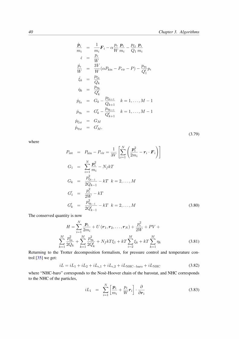
40 Chapter 3. Algorithms
pimi
=1
miF i − α
pεW
pimi− pξ1Q1
pimi
ε =pεW
pεW
=3V
W(αPkin − Pvir − P )− pη1
Q′1pε
ξk =pξkQk
ηk =pηkQ′k
pξk = Gk −pξk+1
Qk+1k = 1, . . . ,M − 1
pηk = G′k −pηk+1
Q′k+1
k = 1, . . . ,M − 1
pξM = GM
pηM = G′M ,
(3.79)
where
Pint = Pkin − Pvir =1
3V
[N∑i=1
(p2i
2mi− ri · F i
)]
G1 =N∑i=1
p2i
mi−NfkT
Gk =p2ξk−1
2Qk−1− kT k = 2, . . . ,M
G′1 =p2ε
2W− kT
G′k =p2ηk−1
2Q′k−1
− kT k = 2, . . . ,M (3.80)
The conserved quantity is now
H =N∑i=1
pi2mi
+ U (r1, r2, . . . , rN ) +p2ε
2W+ PV +
M∑k=1
p2ξk
2Qk+
M∑k=1
p2ηk
2Q′k+NfkTξ1 + kT
M∑i=2
ξk + kTM∑k=1
ηk (3.81)
Returning to the Trotter decomposition formalism, for pressure control and temperature con-trol [35] we get:
iL = iL1 + iL2 + iLε,1 + iLε,2 + iLNHC−baro + iLNHC (3.82)
where “NHC-baro” corresponds to the Nosè-Hoover chain of the barostat, and NHC correspondsto the NHC of the particles,
iL1 =N∑i=1
[pimi
+pεWri
]· ∂∂ri
(3.83)

3.4. Molecular Dynamics 41
iL2 =N∑i=1
F i − αpεWpi ·
∂
∂pi(3.84)
iLε,1 =pεW
∂
∂ε(3.85)
iLε,2 = Gε∂
∂pε(3.86)
and where
Gε = 3V (αPkin − Pvir − P ) (3.87)
Using the Trotter decomposition, we get
exp(iL∆t) = exp (iLNHC−baro∆t/2) exp (iLNHC∆t/2)
exp (iLε,2∆t/2) exp (iL2∆t/2)
exp (iLε,1∆t) exp (iL1∆t)
exp (iL2∆t/2) exp (iLε,2∆t/2)
exp (iLNHC∆t/2) exp (iLNHC−baro∆t/2) +O(∆t3) (3.88)
The action of exp (iL1∆t) comes from the solution of the the differential equation ri = vi + vεriwith vi = pi/mi and vε constant with initial condition ri(0), evaluate at t = ∆t. This yields theevolution
ri(∆t) = ri(0)evε∆t + ∆tvi(0)evε∆t/2sinh (vε∆t/2)
vε∆t/2. (3.89)
The action of exp (iL2∆t/2) comes from the solution of the differential equation vi = F imi−
αvεvi, yielding
vi(∆t/2) = vi(0)e−αvε∆t/2 +∆t
2miF i(0)e−αvε∆t/4
sinh (αvε∆t/4)
αvε∆t/4. (3.90)
md-vv-avek uses the full step kinetic energies for determining the pressure with the pressure con-trol, but the half-step-averaged kinetic energy for the temperatures, which can be written as aTrotter decomposition as
exp(iL∆t) = exp (iLNHC−baro∆t/2) exp (iLε,2∆t/2) exp (iL2∆t/2)
exp (iLNHC∆t/2) exp (iLε,1∆t) exp (iL1∆t) exp (iLNHC∆t/2)
exp (iL2∆t/2) exp (iLε,2∆t/2) exp (iLNHC−baro∆t/2) +O(∆t3)(3.91)
With constraints, the equations become significantly more complicated, in that each of these equa-tions need to be solved iteratively for the constraint forces. Before GROMACS 5.1, these iterativeconstraints were solved as described in [42]. From GROMACS 5.1 onward, MTTK with con-straints has been removed because of numerical stability issues with the iterations.
Infrequent evaluation of temperature and pressure coupling
Temperature and pressure control require global communication to compute the kinetic energy andvirial, which can become costly if performed every step for large systems. We can rearrange the

42 Chapter 3. Algorithms
Trotter decomposition to give alternate symplectic, reversible integrator with the coupling stepsevery n steps instead of every steps. These new integrators will diverge if the coupling time stepis too large, as the auxiliary variable integrations will not converge. However, in most cases, longcoupling times are more appropriate, as they disturb the dynamics less [35].
Standard velocity Verlet with Nosé-Hoover temperature control has a Trotter expansion
exp(iL∆t) ≈ exp (iLNHC∆t/2) exp (iL2∆t/2)
exp (iL1∆t) exp (iL2∆t/2) exp (iLNHC∆t/2) . (3.92)
If the Nosé-Hoover chain is sufficiently slow with respect to the motions of the system, we canwrite an alternate integrator over n steps for velocity Verlet as
exp(iL∆t) ≈ (exp (iLNHC(n∆t/2)) [exp (iL2∆t/2)
exp (iL1∆t) exp (iL2∆t/2)]n exp (iLNHC(n∆t/2)) . (3.93)
For pressure control, this becomes
exp(iL∆t) ≈ exp (iLNHC−baro(n∆t/2)) exp (iLNHC(n∆t/2))
exp (iLε,2(n∆t/2)) [exp (iL2∆t/2)
exp (iLε,1∆t) exp (iL1∆t)
exp (iL2∆t/2)]n exp (iLε,2(n∆t/2))
exp (iLNHC(n∆t/2)) exp (iLNHC−baro(n∆t/2)) , (3.94)
where the box volume integration occurs every step, but the auxiliary variable integrations happenevery n steps.
3.4.10 The complete update algorithm
The complete algorithm for the update of velocities and coordinates is given using leap-frog inFig. 3.8. The SHAKE algorithm of step 4 is explained below.
GROMACS has a provision to “freeze” (prevent motion of) selected particles, which must bedefined as a “freeze group.” This is implemented using a freeze factor fg, which is a vector, anddiffers for each freeze group (see sec. 3.3). This vector contains only zero (freeze) or one (don’tfreeze). When we take this freeze factor and the external acceleration ah into account the updatealgorithm for the velocities becomes
v(t+∆t
2) = fg ∗ λ ∗
[v(t− ∆t
2) +
F (t)
m∆t+ ah∆t
], (3.95)
where g and h are group indices which differ per atom.
3.4.11 Output step
The most important output of the MD run is the trajectory file, which contains particle coordi-nates and (optionally) velocities at regular intervals. The trajectory file contains frames that could

3.4. Molecular Dynamics 43
THE UPDATE ALGORITHM
Given:Positions r of all atoms at time t
Velocities v of all atoms at time t− 12∆t
Accelerations F /m on all atoms at time t.(Forces are computed disregarding any constraints)
Total kinetic energy and virial at t−∆t⇓
1. Compute the scaling factors λ and µaccording to eqns. 3.44 and 3.60
⇓2. Update and scale velocities: v′ = λ(v + a∆t)
⇓3. Compute new unconstrained coordinates: r′ = r + v′∆t
⇓4. Apply constraint algorithm to coordinates: constrain(r
′ → r′′; r)⇓
5. Correct velocities for constraints: v = (r′′ − r)/∆t⇓
6. Scale coordinates and box: r = µr′′; b = µb
Figure 3.8: The MD update algorithm with the leap-frog integrator

44 Chapter 3. Algorithms
include positions, velocities and/or forces, as well as information about the dimensions of the sim-ulation volume, integration step, integration time, etc. The interpretation of the time varies withthe integrator chosen, as described above. For Velocity Verlet integrators, velocities labeled attime t are for that time. For other integrators (e.g. leap-frog, stochastic dynamics), the velocitieslabeled at time t are for time t− 1
2∆t.
Since the trajectory files are lengthy, one should not save every step! To retain all information itsuffices to write a frame every 15 steps, since at least 30 steps are made per period of the highestfrequency in the system, and Shannon’s sampling theorem states that two samples per period ofthe highest frequency in a band-limited signal contain all available information. But that still givesvery long files! So, if the highest frequencies are not of interest, 10 or 20 samples per ps maysuffice. Be aware of the distortion of high-frequency motions by the stroboscopic effect, calledaliasing: higher frequencies are mirrored with respect to the sampling frequency and appear aslower frequencies.
GROMACS can also write reduced-precision coordinates for a subset of the simulation system toa special compressed trajectory file format. All the other tools can read and write this format. Seethe User Guide for details on how to set up your .mdp file to have mdrun use this feature.
3.5 Shell molecular dynamics
GROMACS can simulate polarizability using the shell model of Dick and Overhauser [43]. Insuch models a shell particle representing the electronic degrees of freedom is attached to a nucleusby a spring. The potential energy is minimized with respect to the shell position at every stepof the simulation (see below). Successful applications of shell models in GROMACS have beenpublished for N2 [44] and water [45].
3.5.1 Optimization of the shell positions
The force F S on a shell particle S can be decomposed into two components
F S = F bond + F nb (3.96)
where F bond denotes the component representing the polarization energy, usually represented bya harmonic potential and F nb is the sum of Coulomb and van der Waals interactions. If we assumethat F nb is almost constant we can analytically derive the optimal position of the shell, i.e. whereF S = 0. If we have the shell S connected to atom A we have
F bond = kb (xS − xA) . (3.97)
In an iterative solver, we have positions xS(n) where n is the iteration count. We now have atiteration n
F nb = F S − kb (xS(n)− xA) (3.98)
and the optimal position for the shells xS(n+ 1) thus follows from
F S − kb (xS(n)− xA) + kb (xS(n+ 1)− xA) = 0 (3.99)
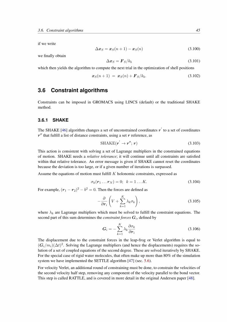
3.6. Constraint algorithms 45
if we write∆xS = xS(n+ 1)− xS(n) (3.100)
we finally obtain∆xS = F S/kb (3.101)
which then yields the algorithm to compute the next trial in the optimization of shell positions
xS(n+ 1) = xS(n) + F S/kb. (3.102)
3.6 Constraint algorithms
Constraints can be imposed in GROMACS using LINCS (default) or the traditional SHAKEmethod.
3.6.1 SHAKE
The SHAKE [46] algorithm changes a set of unconstrained coordinates r′
to a set of coordinatesr′′ that fulfill a list of distance constraints, using a set r reference, as
SHAKE(r′ → r′′; r) (3.103)
This action is consistent with solving a set of Lagrange multipliers in the constrained equationsof motion. SHAKE needs a relative tolerance; it will continue until all constraints are satisfiedwithin that relative tolerance. An error message is given if SHAKE cannot reset the coordinatesbecause the deviation is too large, or if a given number of iterations is surpassed.
Assume the equations of motion must fulfill K holonomic constraints, expressed as
σk(r1 . . . rN ) = 0; k = 1 . . .K. (3.104)
For example, (r1 − r2)2 − b2 = 0. Then the forces are defined as
− ∂
∂ri
(V +
K∑k=1
λkσk
), (3.105)
where λk are Lagrange multipliers which must be solved to fulfill the constraint equations. Thesecond part of this sum determines the constraint forcesGi, defined by
Gi = −K∑k=1
λk∂σk∂ri
(3.106)
The displacement due to the constraint forces in the leap-frog or Verlet algorithm is equal to(Gi/mi)(∆t)
2. Solving the Lagrange multipliers (and hence the displacements) requires the so-lution of a set of coupled equations of the second degree. These are solved iteratively by SHAKE.For the special case of rigid water molecules, that often make up more than 80% of the simulationsystem we have implemented the SETTLE algorithm [47] (sec. 5.6).
For velocity Verlet, an additional round of constraining must be done, to constrain the velocities ofthe second velocity half step, removing any component of the velocity parallel to the bond vector.This step is called RATTLE, and is covered in more detail in the original Andersen paper [48].

46 Chapter 3. Algorithms
unconstrainedupdate
correction forrotational
lengthening
projecting outforces working
along the bonds
θ
d
l d
pd
Figure 3.9: The three position updates needed for one time step. The dashed line is the old bondof length d, the solid lines are the new bonds. l = d cos θ and p = (2d2 − l2)
12 .
3.6.2 LINCS
The LINCS algorithm
LINCS is an algorithm that resets bonds to their correct lengths after an unconstrained update [49].The method is non-iterative, as it always uses two steps. Although LINCS is based on matrices, nomatrix-matrix multiplications are needed. The method is more stable and faster than SHAKE, butit can only be used with bond constraints and isolated angle constraints, such as the proton anglein OH. Because of its stability, LINCS is especially useful for Brownian dynamics. LINCS hastwo parameters, which are explained in the subsection parameters. The parallel version of LINCS,P-LINCS, is described in subsection 3.17.3.
The LINCS formulas
We consider a system of N particles, with positions given by a 3N vector r(t). For moleculardynamics the equations of motion are given by Newton’s Law
d2r
dt2= M−1F , (3.107)
where F is the 3N force vector and M is a 3N × 3N diagonal matrix, containing the masses ofthe particles. The system is constrained by K time-independent constraint equations
gi(r) = |ri1 − ri2 | − di = 0 i = 1, . . . ,K. (3.108)
In a numerical integration scheme, LINCS is applied after an unconstrained update, just likeSHAKE. The algorithm works in two steps (see figure Fig. 3.9). In the first step, the projec-tions of the new bonds on the old bonds are set to zero. In the second step, a correction is appliedfor the lengthening of the bonds due to rotation. The numerics for the first step and the secondstep are very similar. A complete derivation of the algorithm can be found in [49]. Only a shortdescription of the first step is given here.

3.6. Constraint algorithms 47
A new notation is introduced for the gradient matrix of the constraint equations which appears onthe right hand side of this equation:
Bhi =∂gh∂ri
(3.109)
Notice thatB is aK×3N matrix, it contains the directions of the constraints. The following equa-tion shows how the new constrained coordinates rn+1 are related to the unconstrained coordinatesruncn+1 by
rn+1 = (I − T nBn)runcn+1 + T nd =
runcn+1 −M−1Bn(BnM−1BT
n )−1(Bnruncn+1 − d)
(3.110)
where T = M−1BT (BM−1BT )−1. The derivation of this equation from eqns. 3.107 and 3.108can be found in [49].
This first step does not set the real bond lengths to the prescribed lengths, but the projection of thenew bonds onto the old directions of the bonds. To correct for the rotation of bond i, the projectionof the bond, pi, on the old direction is set to
pi =√
2d2i − l2i , (3.111)
where li is the bond length after the first projection. The corrected positions are
r∗n+1 = (I − T nBn)rn+1 + T np. (3.112)
This correction for rotational effects is actually an iterative process, but during MD only oneiteration is applied. The relative constraint deviation after this procedure will be less than 0.0001for every constraint. In energy minimization, this might not be accurate enough, so the number ofiterations is equal to the order of the expansion (see below).
Half of the CPU time goes to inverting the constraint coupling matrix BnM−1BT
n , which has tobe done every time step. ThisK×K matrix has 1/mi1 +1/mi2 on the diagonal. The off-diagonalelements are only non-zero when two bonds are connected, then the element is cosφ/mc, wheremc is the mass of the atom connecting the two bonds and φ is the angle between the bonds.
The matrix T is inverted through a power expansion. A K ×K matrix S is introduced which isthe inverse square root of the diagonal ofBnM
−1BTn . This matrix is used to convert the diagonal
elements of the coupling matrix to one:
(BnM−1BT
n )−1 = SS−1(BnM−1BT
n )−1S−1S
= S(SBnM−1BT
nS)−1S = S(I −An)−1S(3.113)
The matrixAn is symmetric and sparse and has zeros on the diagonal. Thus a simple trick can beused to calculate the inverse:
(I −An)−1 = I +An +A2n +A3
n + . . . (3.114)
This inversion method is only valid if the absolute values of all the eigenvalues of An are smallerthan one. In molecules with only bond constraints, the connectivity is so low that this will alwaysbe true, even if ring structures are present. Problems can arise in angle-constrained molecules. By

48 Chapter 3. Algorithms
constraining angles with additional distance constraints, multiple small ring structures are intro-duced. This gives a high connectivity, leading to large eigenvalues. Therefore LINCS should NOTbe used with coupled angle-constraints.
For molecules with all bonds constrained the eigenvalues of A are around 0.4. This means thatwith each additional order in the expansion eqn. 3.114 the deviations decrease by a factor 0.4. Butfor relatively isolated triangles of constraints the largest eigenvalue is around 0.7. Such trianglescan occur when removing hydrogen angle vibrations with an additional angle constraint in alcoholgroups or when constraining water molecules with LINCS, for instance with flexible constraints.The constraints in such triangles converge twice as slow as the other constraints. Therefore, start-ing with GROMACS 4, additional terms are added to the expansion for such triangles
(I −An)−1 ≈ I +An + . . .+ANin +
(A∗n + . . .+A∗n
Ni)ANin (3.115)
whereNi is the normal order of the expansion andA∗ only contains the elements ofA that coupleconstraints within rigid triangles, all other elements are zero. In this manner, the accuracy of angleconstraints comes close to that of the other constraints, while the series of matrix vector multi-plications required for determining the expansion only needs to be extended for a few constraintcouplings. This procedure is described in the P-LINCS paper[50].
The LINCS Parameters
The accuracy of LINCS depends on the number of matrices used in the expansion eqn. 3.114.For MD calculations a fourth order expansion is enough. For Brownian dynamics with large timesteps an eighth order expansion may be necessary. The order is a parameter in the *.mdp file.The implementation of LINCS is done in such a way that the algorithm will never crash. Evenwhen it is impossible to to reset the constraints LINCS will generate a conformation which fulfillsthe constraints as well as possible. However, LINCS will generate a warning when in one step abond rotates over more than a predefined angle. This angle is set by the user in the *.mdp file.
3.7 Simulated Annealing
The well known simulated annealing (SA) protocol is supported in GROMACS, and you can evencouple multiple groups of atoms separately with an arbitrary number of reference temperaturesthat change during the simulation. The annealing is implemented by simply changing the currentreference temperature for each group in the temperature coupling, so the actual relaxation andcoupling properties depends on the type of thermostat you use and how hard you are coupling it.Since we are changing the reference temperature it is important to remember that the system willNOT instantaneously reach this value - you need to allow for the inherent relaxation time in thecoupling algorithm too. If you are changing the annealing reference temperature faster than thetemperature relaxation you will probably end up with a crash when the difference becomes toolarge.
The annealing protocol is specified as a series of corresponding times and reference temperaturesfor each group, and you can also choose whether you only want a single sequence (after which thetemperature will be coupled to the last reference value), or if the annealing should be periodic and

3.8. Stochastic Dynamics 49
restart at the first reference point once the sequence is completed. You can mix and match bothtypes of annealing and non-annealed groups in your simulation.
3.8 Stochastic Dynamics
Stochastic or velocity Langevin dynamics adds a friction and a noise term to Newton’s equationsof motion, as
mid2ridt2
= −miγidridt
+ F i(r)+ri, (3.116)
where γi is the friction constant [1/ps] andri (t) is a noise process with 〈ri (t)
rj (t + s)〉 =
2miγikBTδ(s)δij . When 1/γi is large compared to the time scales present in the system, onecould see stochastic dynamics as molecular dynamics with stochastic temperature-coupling. Butany processes that take longer than 1/γi, e.g. hydrodynamics, will be dampened. Since each de-gree of freedom is coupled independently to a heat bath, equilibration of fast modes occurs rapidly.For simulating a system in vacuum there is the additional advantage that there is no accumulationof errors for the overall translational and rotational degrees of freedom. When 1/γi is small com-pared to the time scales present in the system, the dynamics will be completely different from MD,but the sampling is still correct.
In GROMACS there is one simple and efficient implementation. Its accuracy is equivalent to thenormal MD leap-frog and Velocity Verlet integrator. It is nearly identical to the common way ofdiscretizing the Langevin equation, but the friction and velocity term are applied in an impulsefashion [51]. It can be described as:
v′ = v(t− 1
2∆t) +
1
mF (t)∆t (3.117)
∆v = −α v′(t+1
2∆t) +
√kBT
m(1− α2) rGi (3.118)
r(t+ ∆t) = r(t) +
(v′ +
1
2∆v
)∆t (3.119)
v(t+1
2∆t) = v′ + ∆v (3.120)
α = 1− e−γ∆t (3.121)
where rGi is Gaussian distributed noise with µ = 0, σ = 1. The velocity is first updated a full timestep without friction and noise to get v′, identical to the normal update in leap-frog. The frictionand noise are then applied as an impulse at step t + ∆t. The advantage of this scheme is that thevelocity-dependent terms act at the full time step, which makes the correct integration of forces thatdepend on both coordinates and velocities, such as constraints and dissipative particle dynamics(DPD, not implented yet), straightforward. With constraints, the coordinate update eqn. 3.119 issplit into a normal leap-frog update and a ∆v. After both of these updates the constraints areapplied to coordinates and velocities.
When using SD as a thermostat, an appropriate value for γ is e.g. 0.5 ps−1, since this results in afriction that is lower than the internal friction of water, while it still provides efficient thermostat-ting.

50 Chapter 3. Algorithms
3.9 Brownian Dynamics
In the limit of high friction, stochastic dynamics reduces to Brownian dynamics, also called po-sition Langevin dynamics. This applies to over-damped systems, i.e. systems in which the inertiaeffects are negligible. The equation is
dridt
=1
γiF i(r)+
ri (3.122)
where γi is the friction coefficient [amu/ps] andri(t) is a noise process with 〈ri(t)
rj(t + s)〉 =
2δ(s)δijkBT/γi. In GROMACS the equations are integrated with a simple, explicit scheme
ri(t+ ∆t) = ri(t) +∆t
γiF i(r(t)) +
√2kBT
∆t
γirGi , (3.123)
where rGi is Gaussian distributed noise with µ = 0, σ = 1. The friction coefficients γi can bechosen the same for all particles or as γi = mi γi, where the friction constants γi can be differentfor different groups of atoms. Because the system is assumed to be over-damped, large timestepscan be used. LINCS should be used for the constraints since SHAKE will not converge for largeatomic displacements. BD is an option of the mdrun program.
3.10 Energy Minimization
Energy minimization in GROMACS can be done using steepest descent, conjugate gradients, or l-bfgs (limited-memory Broyden-Fletcher-Goldfarb-Shanno quasi-Newtonian minimizer...we preferthe abbreviation). EM is just an option of the mdrun program.
3.10.1 Steepest Descent
Although steepest descent is certainly not the most efficient algorithm for searching, it is robustand easy to implement.
We define the vector r as the vector of all 3N coordinates. Initially a maximum displacement h0
(e.g. 0.01 nm) must be given.
First the forces F and potential energy are calculated. New positions are calculated by
rn+1 = rn +F n
max(|F n|)hn, (3.124)
where hn is the maximum displacement and F n is the force, or the negative gradient of the po-tential V . The notation max(|F n|) means the largest scalar force on any atom. The forces andenergy are again computed for the new positionsIf (Vn+1 < Vn) the new positions are accepted and hn+1 = 1.2hn.If (Vn+1 ≥ Vn) the new positions are rejected and hn = 0.2hn.
The algorithm stops when either a user-specified number of force evaluations has been performed(e.g. 100), or when the maximum of the absolute values of the force (gradient) components is

3.11. Normal-Mode Analysis 51
smaller than a specified value ε. Since force truncation produces some noise in the energy evalua-tion, the stopping criterion should not be made too tight to avoid endless iterations. A reasonablevalue for ε can be estimated from the root mean square force f a harmonic oscillator would exhibitat a temperature T . This value is
f = 2πν√
2mkT , (3.125)
where ν is the oscillator frequency, m the (reduced) mass, and k Boltzmann’s constant. For aweak oscillator with a wave number of 100 cm−1 and a mass of 10 atomic units, at a temperatureof 1 K, f = 7.7 kJ mol−1 nm−1. A value for ε between 1 and 10 is acceptable.
3.10.2 Conjugate Gradient
Conjugate gradient is slower than steepest descent in the early stages of the minimization, butbecomes more efficient closer to the energy minimum. The parameters and stop criterion are thesame as for steepest descent. In GROMACS conjugate gradient can not be used with constraints,including the SETTLE algorithm for water [47], as this has not been implemented. If water ispresent it must be of a flexible model, which can be specified in the *.mdp file by define =-DFLEXIBLE.
This is not really a restriction, since the accuracy of conjugate gradient is only required for mini-mization prior to a normal-mode analysis, which cannot be performed with constraints. For mostother purposes steepest descent is efficient enough.
3.10.3 L-BFGS
The original BFGS algorithm works by successively creating better approximations of the inverseHessian matrix, and moving the system to the currently estimated minimum. The memory re-quirements for this are proportional to the square of the number of particles, so it is not practicalfor large systems like biomolecules. Instead, we use the L-BFGS algorithm of Nocedal [52, 53],which approximates the inverse Hessian by a fixed number of corrections from previous steps.This sliding-window technique is almost as efficient as the original method, but the memory re-quirements are much lower - proportional to the number of particles multiplied with the correctionsteps. In practice we have found it to converge faster than conjugate gradients, but due to thecorrection steps it is not yet parallelized. It is also noteworthy that switched or shifted interactionsusually improve the convergence, since sharp cut-offs mean the potential function at the currentcoordinates is slightly different from the previous steps used to build the inverse Hessian approxi-mation.
3.11 Normal-Mode Analysis
Normal-mode analysis [54, 55, 56] can be performed using GROMACS, by diagonalization of themass-weighted Hessian H:
RTM−1/2HM−1/2R = diag(λ1, . . . , λ3N ) (3.126)
λi = (2πωi)2 (3.127)

52 Chapter 3. Algorithms
where M contains the atomic masses, R is a matrix that contains the eigenvectors as columns, λiare the eigenvalues and ωi are the corresponding frequencies.
First the Hessian matrix, which is a 3N × 3N matrix where N is the number of atoms, needs tobe calculated:
Hij =∂2V
∂xi∂xj(3.128)
where xi and xj denote the atomic x, y or z coordinates. In practice, this equation is not used, butthe Hessian is calculated numerically from the force as:
Hij = −fi(x + hej)− fi(x− hej)
2h(3.129)
fi = −∂V∂xi
(3.130)
where ej is the unit vector in direction j. It should be noted that for a usual normal-mode cal-culation, it is necessary to completely minimize the energy prior to computation of the Hessian.The tolerance required depends on the type of system, but a rough indication is 0.001 kJ mol−1.Minimization should be done with conjugate gradients or L-BFGS in double precision.
A number of GROMACS programs are involved in these calculations. First, the energy shouldbe minimized using mdrun. Then, mdrun computes the Hessian. Note that for generating therun input file, one should use the minimized conformation from the full precision trajectory file,as the structure file is not accurate enough. gmx nmeig does the diagonalization and the sortingof the normal modes according to their frequencies. Both mdrun and gmx nmeig should berun in double precision. The normal modes can be analyzed with the program gmx anaeig.Ensembles of structures at any temperature and for any subset of normal modes can be generatedwith gmx nmens. An overview of normal-mode analysis and the related principal componentanalysis (see sec. 8.11) can be found in [57].
3.12 Free energy calculations
3.12.1 Slow-growth methods
Free energy calculations can be performed in GROMACS using a number of methods, including“slow-growth.” An example problem might be calculating the difference in free energy of bindingof an inhibitor I to an enzyme E and to a mutated enzyme E′. It is not feasible with computer sim-ulations to perform a docking calculation for such a large complex, or even releasing the inhibitorfrom the enzyme in a reasonable amount of computer time with reasonable accuracy. However, ifwe consider the free energy cycle in Fig. 3.10A we can write:
∆G1 −∆G2 = ∆G3 −∆G4 (3.131)
If we are interested in the left-hand term we can equally well compute the right-hand term.
If we want to compute the difference in free energy of binding of two inhibitors I and I′ to anenzyme E (Fig. 3.10B) we can again use eqn. 3.131 to compute the desired property.

3.12. Free energy calculations 53
IE’
E IEE
’
G1
∆∆
G2
∆G
4
∆G
3
A
G1
∆∆
G2
∆G
3
II’
E I
E I’
∆G
4
B
Figure 3.10: Free energy cycles. A: to calculate ∆G12, the free energy difference between thebinding of inhibitor I to enzymes E respectively E′. B: to calculate ∆G12, the free energy differ-ence for binding of inhibitors I respectively I′ to enzyme E.
Free energy differences between two molecular species can be calculated in GROMACS usingthe “slow-growth” method. Such free energy differences between different molecular speciesare physically meaningless, but they can be used to obtain meaningful quantities employing athermodynamic cycle. The method requires a simulation during which the Hamiltonian of thesystem changes slowly from that describing one system (A) to that describing the other system(B). The change must be so slow that the system remains in equilibrium during the process; if thatrequirement is fulfilled, the change is reversible and a slow-growth simulation from B to A willyield the same results (but with a different sign) as a slow-growth simulation from A to B. This isa useful check, but the user should be aware of the danger that equality of forward and backwardgrowth results does not guarantee correctness of the results.
The required modification of the Hamiltonian H is realized by making H a function of a couplingparameter λ : H = H(p, q;λ) in such a way that λ = 0 describes system A and λ = 1 describessystem B:
H(p, q; 0) = HA(p, q); H(p, q; 1) = HB(p, q). (3.132)
In GROMACS, the functional form of the λ-dependence is different for the various force-fieldcontributions and is described in section sec. 4.5.
The Helmholtz free energy A is related to the partition function Q of an N,V, T ensemble, whichis assumed to be the equilibrium ensemble generated by a MD simulation at constant volume andtemperature. The generally more useful Gibbs free energy G is related to the partition function∆ of an N, p, T ensemble, which is assumed to be the equilibrium ensemble generated by a MDsimulation at constant pressure and temperature:
A(λ) = −kBT lnQ (3.133)
Q = c
∫ ∫exp[−βH(p, q;λ)] dp dq (3.134)
G(λ) = −kBT ln ∆ (3.135)
∆ = c
∫ ∫ ∫exp[−βH(p, q;λ)− βpV ] dp dq dV (3.136)
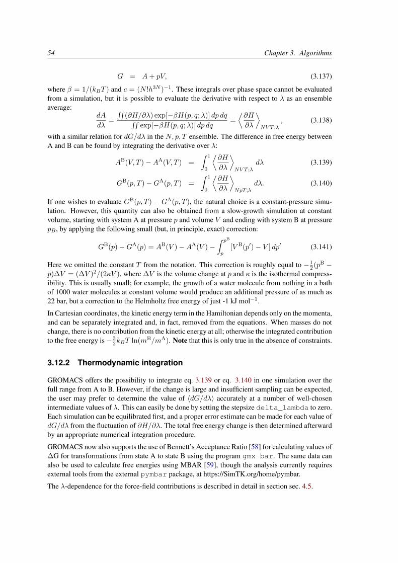
54 Chapter 3. Algorithms
G = A+ pV, (3.137)
where β = 1/(kBT ) and c = (N !h3N )−1. These integrals over phase space cannot be evaluatedfrom a simulation, but it is possible to evaluate the derivative with respect to λ as an ensembleaverage:
dA
dλ=
∫∫(∂H/∂λ) exp[−βH(p, q;λ)] dp dq∫∫
exp[−βH(p, q;λ)] dp dq=
⟨∂H
∂λ
⟩NV T ;λ
, (3.138)
with a similar relation for dG/dλ in the N, p, T ensemble. The difference in free energy betweenA and B can be found by integrating the derivative over λ:
AB(V, T )−AA(V, T ) =
∫ 1
0
⟨∂H
∂λ
⟩NV T ;λ
dλ (3.139)
GB(p, T )−GA(p, T ) =
∫ 1
0
⟨∂H
∂λ
⟩NpT ;λ
dλ. (3.140)
If one wishes to evaluate GB(p, T ) − GA(p, T ), the natural choice is a constant-pressure simu-lation. However, this quantity can also be obtained from a slow-growth simulation at constantvolume, starting with system A at pressure p and volume V and ending with system B at pressurepB , by applying the following small (but, in principle, exact) correction:
GB(p)−GA(p) = AB(V )−AA(V )−∫ pB
p[V B(p′)− V ] dp′ (3.141)
Here we omitted the constant T from the notation. This correction is roughly equal to −12(pB −
p)∆V = (∆V )2/(2κV ), where ∆V is the volume change at p and κ is the isothermal compress-ibility. This is usually small; for example, the growth of a water molecule from nothing in a bathof 1000 water molecules at constant volume would produce an additional pressure of as much as22 bar, but a correction to the Helmholtz free energy of just -1 kJ mol−1.
In Cartesian coordinates, the kinetic energy term in the Hamiltonian depends only on the momenta,and can be separately integrated and, in fact, removed from the equations. When masses do notchange, there is no contribution from the kinetic energy at all; otherwise the integrated contributionto the free energy is−3
2kBT ln(mB/mA). Note that this is only true in the absence of constraints.
3.12.2 Thermodynamic integration
GROMACS offers the possibility to integrate eq. 3.139 or eq. 3.140 in one simulation over thefull range from A to B. However, if the change is large and insufficient sampling can be expected,the user may prefer to determine the value of 〈dG/dλ〉 accurately at a number of well-chosenintermediate values of λ. This can easily be done by setting the stepsize delta_lambda to zero.Each simulation can be equilibrated first, and a proper error estimate can be made for each value ofdG/dλ from the fluctuation of ∂H/∂λ. The total free energy change is then determined afterwardby an appropriate numerical integration procedure.
GROMACS now also supports the use of Bennett’s Acceptance Ratio [58] for calculating values of∆G for transformations from state A to state B using the program gmx bar. The same data canalso be used to calculate free energies using MBAR [59], though the analysis currently requiresexternal tools from the external pymbar package, at https://SimTK.org/home/pymbar.
The λ-dependence for the force-field contributions is described in detail in section sec. 4.5.

3.13. Replica exchange 55
3.13 Replica exchange
Replica exchange molecular dynamics (REMD) is a method that can be used to speed up the sam-pling of any type of simulation, especially if conformations are separated by relatively high energybarriers. It involves simulating multiple replicas of the same system at different temperatures andrandomly exchanging the complete state of two replicas at regular intervals with the probability:
P (1↔ 2) = min
(1, exp
[(1
kBT1− 1
kBT2
)(U1 − U2)
])(3.142)
where T1 and T2 are the reference temperatures and U1 and U2 are the instantaneous potentialenergies of replicas 1 and 2 respectively. After exchange the velocities are scaled by (T1/T2)±0.5
and a neighbor search is performed the next step. This combines the fast sampling and frequentbarrier-crossing of the highest temperature with correct Boltzmann sampling at all the differenttemperatures [60, 61]. We only attempt exchanges for neighboring temperatures as the probabilitydecreases very rapidly with the temperature difference. One should not attempt exchanges forall possible pairs in one step. If, for instance, replicas 1 and 2 would exchange, the chance ofexchange for replicas 2 and 3 not only depends on the energies of replicas 2 and 3, but also on theenergy of replica 1. In GROMACS this is solved by attempting exchange for all “odd” pairs on“odd” attempts and for all “even” pairs on “even” attempts. If we have four replicas: 0, 1, 2 and 3,ordered in temperature and we attempt exchange every 1000 steps, pairs 0-1 and 2-3 will be triedat steps 1000, 3000 etc. and pair 1-2 at steps 2000, 4000 etc.
How should one choose the temperatures? The energy difference can be written as:
U1 − U2 = Ndfc
2kB(T1 − T2) (3.143)
where Ndf is the total number of degrees of freedom of one replica and c is 1 for harmonic poten-tials and around 2 for protein/water systems. If T2 = (1 + ε)T1 the probability becomes:
P (1↔ 2) = exp
(− ε2cNdf
2(1 + ε)
)≈ exp
(−ε2 c
2Ndf
)(3.144)
Thus for a probability of e−2 ≈ 0.135 one obtains ε ≈ 2/√cNdf . With all bonds constrained one
has Ndf ≈ 2Natoms and thus for c = 2 one should choose ε as 1/√Natoms. However there is one
problem when using pressure coupling. The density at higher temperatures will decrease, leadingto higher energy [62], which should be taken into account. The GROMACS website features a so-called “REMD calculator,” that lets you type in the temperature range and the number of atoms,and based on that proposes a set of temperatures.
An extension to the REMD for the isobaric-isothermal ensemble was proposed by Okabe etal. [63]. In this work the exchange probability is modified to:
P (1↔ 2) = min
(1, exp
[(1
kBT1− 1
kBT2
)(U1 − U2) +
(P1
kBT1− P2
kBT2
)(V1 − V2)
])(3.145)
where P1 and P2 are the respective reference pressures and V1 and V2 are the respective instanta-neous volumes in the simulations. In most cases the differences in volume are so small that thesecond term is negligible. It only plays a role when the difference between P1 and P2 is large orin phase transitions.
56 Chapter 3. Algorithms
Hamiltonian replica exchange is also supported in GROMACS. In Hamiltonian replica exchange,each replica has a different Hamiltonian, defined by the free energy pathway specified for thesimulation. The exchange probability to maintain the correct ensemble probabilities is:
P (1↔ 2) = min
(1, exp
[(1
kBT− 1
kBT
)((U1(x2)− U1(x1)) + (U2(x1)− U2(x2)))
])(3.146)
The separate Hamiltonians are defined by the free energy functionality of GROMACS, with swapsmade between the different values of λ defined in the mdp file.
Hamiltonian and temperature replica exchange can also be performed simultaneously, using theacceptance criteria:
P (1↔ 2) = min
(1, exp
[(1
kBT−)
(U1(x2)− U1(x1)
kBT1+U2(x1)− U2(x2)
kBT2)
])(3.147)
Gibbs sampling replica exchange has also been implemented in GROMACS [64]. In Gibbs sam-pling replica exchange, all possible pairs are tested for exchange, allowing swaps between replicasthat are not neighbors.
Gibbs sampling replica exchange requires no additional potential energy calculations. Howeverthere is an additional communication cost in Gibbs sampling replica exchange, as for some permu-tations, more than one round of swaps must take place. In some cases, this extra communicationcost might affect the efficiency.
All replica exchange variants are options of the mdrun program. It will only work when MPI isinstalled, due to the inherent parallelism in the algorithm. For efficiency each replica can run on aseparate rank. See the manual page of mdrun on how to use these multinode features.
3.14 Essential Dynamics sampling
The results from Essential Dynamics (see sec. 8.11) of a protein can be used to guide MD sim-ulations. The idea is that from an initial MD simulation (or from other sources) a definition ofthe collective fluctuations with largest amplitude is obtained. The position along one or more ofthese collective modes can be constrained in a (second) MD simulation in a number of ways forseveral purposes. For example, the position along a certain mode may be kept fixed to monitorthe average force (free-energy gradient) on that coordinate in that position. Another applicationis to enhance sampling efficiency with respect to usual MD [65, 66]. In this case, the system isencouraged to sample its available configuration space more systematically than in a diffusion-likepath that proteins usually take.
Another possibility to enhance sampling is flooding. Here a flooding potential is added to certain(collective) degrees of freedom to expel the system out of a region of phase space [67].
The procedure for essential dynamics sampling or flooding is as follows. First, the eigenvectorsand eigenvalues need to be determined using covariance analysis (gmx covar) or normal-modeanalysis (gmx nmeig). Then, this information is fed into make_edi, which has many optionsfor selecting vectors and setting parameters, see gmx make_edi -h. The generated edi inputfile is then passed to mdrun.

3.15. Expanded Ensemble 57
3.15 Expanded Ensemble
In an expanded ensemble simulation [68], both the coordinates and the thermodynamic ensembleare treated as configuration variables that can be sampled over. The probability of any given statecan be written as:
P (~x, k) ∝ exp (−βkUk + gk) , (3.148)
where βk = 1kBTk
is the β corresponding to the kth thermodynamic state, and gk is a user-specifiedweight factor corresponding to the kth state. This space is therefore a mixed, generalized, orexpanded ensemble which samples from multiple thermodynamic ensembles simultaneously. gkis chosen to give a specific weighting of each subensemble in the expanded ensemble, and caneither be fixed, or determined by an iterative procedure. The set of gk is frequently chosen togive each thermodynamic ensemble equal probability, in which case gk is equal to the free energyin non-dimensional units, but they can be set to arbitrary values as desired. Several differentalgorithms can be used to equilibrate these weights, described in the mdp option listings.
In GROMACS, this space is sampled by alternating sampling in the k and ~x directions. Samplingin the ~x direction is done by standard molecular dynamics sampling; sampling between the dif-ferent thermodynamics states is done by Monte Carlo, with several different Monte Carlo movessupported. The k states can be defined by different temperatures, or choices of the free energyλ variable, or both. Expanded ensemble simulations thus represent a serialization of the replicaexchange formalism, allowing a single simulation to explore many thermodynamic states.
3.16 Parallelization
The CPU time required for a simulation can be reduced by running the simulation in parallel overmore than one core. Ideally, one would want to have linear scaling: running on N cores makesthe simulation N times faster. In practice this can only be achieved for a small number of cores.The scaling will depend a lot on the algorithms used. Also, different algorithms can have differentrestrictions on the interaction ranges between atoms.
3.17 Domain decomposition
Since most interactions in molecular simulations are local, domain decomposition is a natural wayto decompose the system. In domain decomposition, a spatial domain is assigned to each rank,which will then integrate the equations of motion for the particles that currently reside in its localdomain. With domain decomposition, there are two choices that have to be made: the division ofthe unit cell into domains and the assignment of the forces to domains. Most molecular simulationpackages use the half-shell method for assigning the forces. But there are two methods that alwaysrequire less communication: the eighth shell [69] and the midpoint [70] method. GROMACScurrently uses the eighth shell method, but for certain systems or hardware architectures it mightbe advantageous to use the midpoint method. Therefore, we might implement the midpoint methodin the future. Most of the details of the domain decomposition can be found in the GROMACS 4paper [5].

58 Chapter 3. Algorithms
7
30
4cr
1
65
Figure 3.11: A non-staggered domain decomposition grid of 3×2×2 cells. Coordinates in zones1 to 7 are communicated to the corner cell that has its home particles in zone 0. rc is the cut-offradius.
3.17.1 Coordinate and force communication
In the most general case of a triclinic unit cell, the space in divided with a 1-, 2-, or 3-D grid inparallelepipeds that we call domain decomposition cells. Each cell is assigned to a particle-particlerank. The system is partitioned over the ranks at the beginning of each MD step in which neighborsearching is performed. Since the neighbor searching is based on charge groups, charge groupsare also the units for the domain decomposition. Charge groups are assigned to the cell wheretheir center of geometry resides. Before the forces can be calculated, the coordinates from someneighboring cells need to be communicated, and after the forces are calculated, the forces needto be communicated in the other direction. The communication and force assignment is based onzones that can cover one or multiple cells. An example of a zone setup is shown in Fig. 3.11.
The coordinates are communicated by moving data along the “negative” direction in x, y or zto the next neighbor. This can be done in one or multiple pulses. In Fig. 3.11 two pulses in xare required, then one in y and then one in z. The forces are communicated by reversing thisprocedure. See the GROMACS 4 paper [5] for details on determining which non-bonded andbonded forces should be calculated on which rank.
3.17.2 Dynamic load balancing
When different ranks have a different computational load (load imbalance), all ranks will have towait for the one that takes the most time. One would like to avoid such a situation. Load imbalancecan occur due to four reasons:
• inhomogeneous particle distribution
• inhomogeneous interaction cost distribution (charged/uncharged, water/non-water due toGROMACS water innerloops)

3.17. Domain decomposition 59
11
2d
0
3 2
3’
rc
rb2’
Figure 3.12: The zones to communicate to the rank of zone 0, see the text for details. rc and rbare the non-bonded and bonded cut-off radii respectively, d is an example of a distance betweenfollowing, staggered boundaries of cells.
• statistical fluctuation (only with small particle numbers)
• differences in communication time, due to network topology and/or other jobs on the ma-chine interfering with our communication
So we need a dynamic load balancing algorithm where the volume of each domain decompositioncell can be adjusted independently. To achieve this, the 2- or 3-D domain decomposition gridsneed to be staggered. Fig. 3.12 shows the most general case in 2-D. Due to the staggering, onemight require two distance checks for deciding if a charge group needs to be communicated: anon-bonded distance and a bonded distance check.
By default, mdrun automatically turns on the dynamic load balancing during a simulation whenthe total performance loss due to the force calculation imbalance is 2% or more. Note that thereported force load imbalance numbers might be higher, since the force calculation is only part ofwork that needs to be done during an integration step. The load imbalance is reported in the logfile at log output steps and when the -v option is used also on screen. The average load imbalanceand the total performance loss due to load imbalance are reported at the end of the log file.
There is one important parameter for the dynamic load balancing, which is the minimum allowedscaling. By default, each dimension of the domain decomposition cell can scale down by at leasta factor of 0.8. For 3-D domain decomposition this allows cells to change their volume by about afactor of 0.5, which should allow for compensation of a load imbalance of 100%. The minimumallowed scaling can be changed with the -dds option of mdrun.
The load imbalance is measured by timing a single region of the MD step on each MPI rank. Thisregion can not include MPI communication, as timing of MPI calls does not allow separating waitdue to imbalance from actual communication. The domain volumes are then scaled, with under-relaxation, inversely proportional with the measured time. This procedure will decrease the loadimbalance when the change in load in the measured region correlates with the change in domainvolume and the load outside the measured region does not depend strongly on the domain volume.In CPU-only simulations, the load is measured between the coordinate and the force communica-tion. In simulations with non-bonded work on GPUs, we overlap communication and work on the

60 Chapter 3. Algorithms
interaction range option defaultnon-bonded rc = max(rlist,rVdW,rCoul) mdp file
two-body bonded max(rmb,rc) mdrun -rdd starting conf. + 10%multi-body bonded rmb mdrun -rdd starting conf. + 10%
constraints rcon mdrun -rcon est. from bond lengthsvirtual sites rcon mdrun -rcon 0
Table 3.2: The interaction ranges with domain decomposition.
CPU with calculation on the GPU. Therefore we measure from the last communication before theforce calculation to when the CPU or GPU is finished, whichever is last. When not using PMEranks, we subtract the time in PME from the CPU time, as this includes MPI calls and the PMEload is independent of domain size. This generally works well, unless the non-bonded load islow and there is imbalance in the bonded interactions. Then two issues can arise. Dynamic loadbalancing can increase the imbalance in update and constraints and with PME the coordinate andforce redistribution time can go up significantly. Although dynamic load balancing can signifi-cantly improve performance in cases where there is imbalance in the bonded interactions on theCPU, there are many situations in which some domains continue decreasing in size and the loadimbalance increases and/or PME coordinate and force redistribution cost increases significantly.As of version 2016.1, mdrun disables the dynamic load balancing when measurement indicatesthat it deteriorates performance. This means that in most cases the user will get good performancewith the default, automated dynamic load balancing setting.
3.17.3 Constraints in parallel
Since with domain decomposition parts of molecules can reside on different ranks, bond con-straints can cross cell boundaries. Therefore a parallel constraint algorithm is required. GRO-MACS uses the P-LINCS algorithm [50], which is the parallel version of the LINCS algorithm [49](see 3.6.2). The P-LINCS procedure is illustrated in Fig. 3.13. When molecules cross the cellboundaries, atoms in such molecules up to (lincs_order + 1) bonds away are communi-cated over the cell boundaries. Then, the normal LINCS algorithm can be applied to the localbonds plus the communicated ones. After this procedure, the local bonds are correctly constrained,even though the extra communicated ones are not. One coordinate communication step is requiredfor the initial LINCS step and one for each iteration. Forces do not need to be communicated.
3.17.4 Interaction ranges
Domain decomposition takes advantage of the locality of interactions. This means that there willbe limitations on the range of interactions. By default, mdrun tries to find the optimal balancebetween interaction range and efficiency. But it can happen that a simulation stops with an errormessage about missing interactions, or that a simulation might run slightly faster with shorterinteraction ranges. A list of interaction ranges and their default values is given in Table 3.2.
In most cases the defaults of mdrun should not cause the simulation to stop with an error messageof missing interactions. The range for the bonded interactions is determined from the distance be-
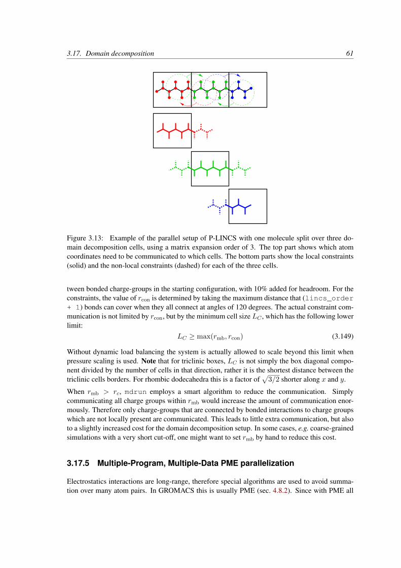
3.17. Domain decomposition 61
Figure 3.13: Example of the parallel setup of P-LINCS with one molecule split over three do-main decomposition cells, using a matrix expansion order of 3. The top part shows which atomcoordinates need to be communicated to which cells. The bottom parts show the local constraints(solid) and the non-local constraints (dashed) for each of the three cells.
tween bonded charge-groups in the starting configuration, with 10% added for headroom. For theconstraints, the value of rcon is determined by taking the maximum distance that (lincs_order+ 1) bonds can cover when they all connect at angles of 120 degrees. The actual constraint com-munication is not limited by rcon, but by the minimum cell size LC , which has the following lowerlimit:
LC ≥ max(rmb, rcon) (3.149)
Without dynamic load balancing the system is actually allowed to scale beyond this limit whenpressure scaling is used. Note that for triclinic boxes, LC is not simply the box diagonal compo-nent divided by the number of cells in that direction, rather it is the shortest distance between thetriclinic cells borders. For rhombic dodecahedra this is a factor of
√3/2 shorter along x and y.
When rmb > rc, mdrun employs a smart algorithm to reduce the communication. Simplycommunicating all charge groups within rmb would increase the amount of communication enor-mously. Therefore only charge-groups that are connected by bonded interactions to charge groupswhich are not locally present are communicated. This leads to little extra communication, but alsoto a slightly increased cost for the domain decomposition setup. In some cases, e.g. coarse-grainedsimulations with a very short cut-off, one might want to set rmb by hand to reduce this cost.
3.17.5 Multiple-Program, Multiple-Data PME parallelization
Electrostatics interactions are long-range, therefore special algorithms are used to avoid summa-tion over many atom pairs. In GROMACS this is usually PME (sec. 4.8.2). Since with PME all

62 Chapter 3. Algorithms
6 PP ranks 2 PME ranks8 PP/PME ranks
Figure 3.14: Example of 8 ranks without (left) and with (right) MPMD. The PME communication(red arrows) is much higher on the left than on the right. For MPMD additional PP - PME coordi-nate and force communication (blue arrows) is required, but the total communication complexityis lower.
particles interact with each other, global communication is required. This will usually be the lim-iting factor for scaling with domain decomposition. To reduce the effect of this problem, we havecome up with a Multiple-Program, Multiple-Data approach [5]. Here, some ranks are selected todo only the PME mesh calculation, while the other ranks, called particle-particle (PP) ranks, doall the rest of the work. For rectangular boxes the optimal PP to PME rank ratio is usually 3:1,for rhombic dodecahedra usually 2:1. When the number of PME ranks is reduced by a factor of4, the number of communication calls is reduced by about a factor of 16. Or put differently, wecan now scale to 4 times more ranks. In addition, for modern 4 or 8 core machines in a network,the effective network bandwidth for PME is quadrupled, since only a quarter of the cores will beusing the network connection on each machine during the PME calculations.
mdrunwill by default interleave the PP and PME ranks. If the ranks are not number consecutivelyinside the machines, one might want to use mdrun -ddorder pp_pme. For machines with areal 3-D torus and proper communication software that assigns the ranks accordingly one shoulduse mdrun -ddorder cartesian.
To optimize the performance one should usually set up the cut-offs and the PME grid such thatthe PME load is 25 to 33% of the total calculation load. grompp will print an estimate for thisload at the end and also mdrun calculates the same estimate to determine the optimal numberof PME ranks to use. For high parallelization it might be worthwhile to optimize the PME loadwith the mdp settings and/or the number of PME ranks with the -npme option of mdrun. Forchanging the electrostatics settings it is useful to know the accuracy of the electrostatics remainsnearly constant when the Coulomb cut-off and the PME grid spacing are scaled by the same factor.Note that it is usually better to overestimate than to underestimate the number of PME ranks, sincethe number of PME ranks is smaller than the number of PP ranks, which leads to less total waitingtime.
The PME domain decomposition can be 1-D or 2-D along the x and/or y axis. 2-D decompositionis also known as pencil decomposition because of the shape of the domains at high parallelization.1-D decomposition along the y axis can only be used when the PP decomposition has only 1 do-main along x. 2-D PME decomposition has to have the number of domains along x equal to thenumber of the PP decomposition. mdrun automatically chooses 1-D or 2-D PME decomposition(when possible with the total given number of ranks), based on the minimum amount of commu-

3.18. Implicit solvation 63
nication for the coordinate redistribution in PME plus the communication for the grid overlap andtransposes. To avoid superfluous communication of coordinates and forces between the PP andPME ranks, the number of DD cells in the x direction should ideally be the same or a multiple ofthe number of PME ranks. By default, mdrun takes care of this issue.
3.17.6 Domain decomposition flow chart
In Fig. 3.15 a flow chart is shown for domain decomposition with all possible communication fordifferent algorithms. For simpler simulations, the same flow chart applies, without the algorithmsand communication for the algorithms that are not used.
3.18 Implicit solvation
Implicit solvent models provide an efficient way of representing the electrostatic effects of solventmolecules, while saving a large piece of the computations involved in an accurate, aqueous de-scription of the surrounding water in molecular dynamics simulations. Implicit solvation modelsoffer several advantages compared with explicit solvation, including eliminating the need for theequilibration of water around the solute, and the absence of viscosity, which allows the protein tomore quickly explore conformational space.
Implicit solvent calculations in GROMACS can be done using the generalized Born-formalism,and the Still [71], HCT [72], and OBC [73] models are available for calculating the Born radii.
Here, the free energy Gsolv of solvation is the sum of three terms, a solvent-solvent cavity term(Gcav), a solute-solvent van der Waals term (Gvdw), and finally a solvent-solute electrostaticspolarization term (Gpol).
The sum of Gcav and Gvdw corresponds to the (non-polar) free energy of solvation for a moleculefrom which all charges have been removed, and is commonly called Gnp, calculated from thetotal solvent accessible surface area multiplied with a surface tension. The total expression for thesolvation free energy then becomes:
Gsolv = Gnp +Gpol (3.150)
Under the generalized Born model, Gpol is calculated from the generalized Born equation [71]:
Gpol =
(1− 1
ε
) n∑i=1
n∑j>i
qiqj√r2ij + bibj exp
(−r2ij4bibj
) (3.151)
In GROMACS, we have introduced the substitution [74]:
ci =1√bi
(3.152)
which makes it possible to introduce a cheap transformation to a new variable x when evaluatingeach interaction, such that:

64 Chapter 3. Algorithms
Figure 3.15: Flow chart showing the algorithms and communication (arrows) for a standard MDsimulation with virtual sites, constraints and separate PME-mesh ranks.

3.18. Implicit solvation 65
x =rij√bibj
= rijcicj (3.153)
In the end, the full re-formulation of 3.151 becomes:
Gpol =
(1− 1
ε
) n∑i=1
n∑j>i
qiqj√bibj
ξ(x) =
(1− 1
ε
) n∑i=1
qici
n∑j>i
qjcj ξ(x) (3.154)
The non-polar part (Gnp) of Equation 3.150 is calculated directly from the Born radius of eachatom using a simple ACE type approximation by Schaefer et al. [75], including a simple loopover all atoms. This requires only one extra solvation parameter, independent of atom type, butdiffering slightly between the three Born radii models.

66 Chapter 3. Algorithms

Chapter 4
Interaction function and forcefields
To accommodate the potential functions used in some popular force fields (see 4.10), GROMACSoffers a choice of functions, both for non-bonded interaction and for dihedral interactions. Theyare described in the appropriate subsections.
The potential functions can be subdivided into three parts
1. Non-bonded: Lennard-Jones or Buckingham, and Coulomb or modified Coulomb. The non-bonded interactions are computed on the basis of a neighbor list (a list of non-bonded atomswithin a certain radius), in which exclusions are already removed.
2. Bonded: covalent bond-stretching, angle-bending, improper dihedrals, and proper dihedrals.These are computed on the basis of fixed lists.
3. Restraints: position restraints, angle restraints, distance restraints, orientation restraints anddihedral restraints, all based on fixed lists.
4. Applied Forces: externally applied forces, see chapter 6.
4.1 Non-bonded interactions
Non-bonded interactions in GROMACS are pair-additive:
V (r1, . . . rN ) =∑i<j
Vij(rij); (4.1)
F i = −∑j
dVij(rij)
drij
rijrij
(4.2)
Since the potential only depends on the scalar distance, interactions will be centro-symmetric,i.e. the vectorial partial force on particle i from the pairwise interaction Vij(rij) has the opposite

68 Chapter 4. Interaction function and force fields
0.4 0.5 0.6 0.7 0.8r (nm)
–0.2
0.0
0.2
0.4
V (
kJ m
ole–1
)
Figure 4.1: The Lennard-Jones interaction.
direction of the partial force on particle j. For efficiency reasons, interactions are calculatedby loops over interactions and updating both partial forces rather than summing one completenonbonded force at a time. The non-bonded interactions contain a repulsion term, a dispersionterm, and a Coulomb term. The repulsion and dispersion term are combined in either the Lennard-Jones (or 6-12 interaction), or the Buckingham (or exp-6 potential). In addition, (partially) chargedatoms act through the Coulomb term.
4.1.1 The Lennard-Jones interaction
The Lennard-Jones potential VLJ between two atoms equals:
VLJ(rij) =C
(12)ij
r12ij
−C
(6)ij
r6ij
(4.3)
See also Fig. 4.1 The parameters C(12)ij and C(6)
ij depend on pairs of atom types; consequently theyare taken from a matrix of LJ-parameters. In the Verlet cut-off scheme, the potential is shifted bya constant such that it is zero at the cut-off distance.
The force derived from this potential is:
F i(rij) =
12C
(12)ij
r13ij
− 6C
(6)ij
r7ij
rijrij
(4.4)
The LJ potential may also be written in the following form:
VLJ(rij) = 4εij
(σijrij
)12
−(σijrij
)6 (4.5)
In constructing the parameter matrix for the non-bonded LJ-parameters, two types of combinationrules can be used within GROMACS, only geometric averages (type 1 in the input section of the

4.1. Non-bonded interactions 69
0.2 0.3 0.4 0.5 0.6 0.7 0.8r (nm)
–0.5
0.0
0.5
1.0
1.5
V (
kJ m
ole–1
)
Figure 4.2: The Buckingham interaction.
force-field file):
C(6)ij =
(C
(6)ii C
(6)jj
)1/2
C(12)ij =
(C
(12)ii C
(12)jj
)1/2 (4.6)
or, alternatively the Lorentz-Berthelot rules can be used. An arithmetic average is used to calculateσij , while a geometric average is used to calculate εij (type 2):
σij = 12(σii + σjj)
εij = (εii εjj)1/2 (4.7)
finally an geometric average for both parameters can be used (type 3):
σij = (σii σjj)1/2
εij = (εii εjj)1/2 (4.8)
This last rule is used by the OPLS force field.
4.1.2 Buckingham potential
The Buckingham potential has a more flexible and realistic repulsion term than the Lennard-Jonesinteraction, but is also more expensive to compute. The potential form is:
Vbh(rij) = Aij exp(−Bijrij)−Cijr6ij
(4.9)
See also Fig. 4.2. The force derived from this is:
F i(rij) =
[AijBij exp(−Bijrij)− 6
Cijr7ij
]rijrij
(4.10)

70 Chapter 4. Interaction function and force fields
0.0 0.2 0.4 0.6 0.8 1.0
r (nm)
0
500
1000
1500
V (
kJ m
ol−
1)
Coulomb
With RF
RF − C
Figure 4.3: The Coulomb interaction (for particles with equal signed charge) with and withoutreaction field. In the latter case εr was 1, εrf was 78, and rc was 0.9 nm. The dot-dashed line isthe same as the dashed line, except for a constant.
4.1.3 Coulomb interaction
The Coulomb interaction between two charge particles is given by:
Vc(rij) = fqiqjεrrij
(4.11)
See also Fig. 4.3, where f = 14πε0
= 138.935 458 (see chapter 2)
The force derived from this potential is:
F i(rij) = fqiqjεrr2
ij
rijrij
(4.12)
A plain Coulomb interaction should only be used without cut-off or when all pairs fall within thecut-off, since there is an abrupt, large change in the force at the cut-off. In case you do want to usea cut-off, the potential can be shifted by a constant to make the potential the integral of the force.With the group cut-off scheme, this shift is only applied to non-excluded pairs. With the Verletcut-off scheme, the shift is also applied to excluded pairs and self interactions, which makes thepotential equivalent to a reaction field with εrf = 1 (see below).
In GROMACS the relative dielectric constant εr may be set in the in the input for grompp.
4.1.4 Coulomb interaction with reaction field
The Coulomb interaction can be modified for homogeneous systems by assuming a constant di-electric environment beyond the cut-off rc with a dielectric constant of εrf . The interaction thenreads:
Vcrf = fqiqjεrrij
[1 +
εrf − εr2εrf + εr
r3ij
r3c
]− f qiqj
εrrc
3εrf2εrf + εr
(4.13)

4.1. Non-bonded interactions 71
in which the constant expression on the right makes the potential zero at the cut-off rc. For chargedcut-off spheres this corresponds to neutralization with a homogeneous background charge. We canrewrite eqn. 4.13 for simplicity as
Vcrf = fqiqjεr
[1
rij+ krf r
2ij − crf
](4.14)
with
krf =1
r3c
εrf − εr(2εrf + εr)
(4.15)
crf =1
rc+ krf r
2c =
1
rc
3εrf(2εrf + εr)
(4.16)
For large εrf the krf goes to r−3c /2, while for εrf = εr the correction vanishes. In Fig. 4.3 the
modified interaction is plotted, and it is clear that the derivative with respect to rij (= -force) goesto zero at the cut-off distance. The force derived from this potential reads:
F i(rij) = fqiqjεr
[1
r2ij
− 2krfrij
]rijrij
(4.17)
The reaction-field correction should also be applied to all excluded atoms pairs, including selfpairs, in which case the normal Coulomb term in eqns. 4.13 and 4.17 is absent.
Tironi et al. have introduced a generalized reaction field in which the dielectric continuum beyondthe cut-off rc also has an ionic strength I [76]. In this case we can rewrite the constants krf andcrf using the inverse Debye screening length κ:
κ2 =2I F 2
ε0εrfRT=
F 2
ε0εrfRT
K∑i=1
ciz2i (4.18)
krf =1
r3c
(εrf − εr)(1 + κrc) + 12εrf (κrc)
2
(2εrf + εr)(1 + κrc) + εrf (κrc)2(4.19)
crf =1
rc
3εrf (1 + κrc + 12(κrc)
2)
(2εrf + εr)(1 + κrc) + εrf (κrc)2(4.20)
where F is Faraday’s constant, R is the ideal gas constant, T the absolute temperature, ci themolar concentration for species i and zi the charge number of species i where we haveK differentspecies. In the limit of zero ionic strength (κ = 0) eqns. 4.19 and 4.20 reduce to the simple formsof eqns. 4.15 and 4.16 respectively.
4.1.5 Modified non-bonded interactions
In GROMACS, the non-bonded potentials can be modified by a shift function, also called a force-switch function, since it switches the force to zero at the cut-off. The purpose of this is to replacethe truncated forces by forces that are continuous and have continuous derivatives at the cut-offradius. With such forces the time integration produces smaller errors. But note that for Lennard-Jones interactions these errors are usually smaller than other errors, such as integration errors at

72 Chapter 4. Interaction function and force fields
the repulsive part of the potential. For Coulomb interactions we advise against using a shiftedpotential and for use of a reaction field or a proper long-range method such as PME.
There is no fundamental difference between a switch function (which multiplies the potential witha function) and a shift function (which adds a function to the force or potential) [77]. The switchfunction is a special case of the shift function, which we apply to the force function F (r), relatedto the electrostatic or van der Waals force acting on particle i by particle j as:
F i = c F (rij)rijrij
(4.21)
For pure Coulomb or Lennard-Jones interactions F (r) = Fα(r) = α r−(α+1). The switched forceFs(r) can generally be written as:
Fs(r) = Fα(r) r < r1
Fs(r) = Fα(r) + S(r) r1 ≤ r < rc
Fs(r) = 0 rc ≤ r
(4.22)
When r1 = 0 this is a traditional shift function, otherwise it acts as a switch function. Thecorresponding shifted potential function then reads:
Vs(r) =
∫ ∞r
Fs(x) dx (4.23)
The GROMACS force switch function SF (r) should be smooth at the boundaries, therefore thefollowing boundary conditions are imposed on the switch function:
SF (r1) = 0S′F (r1) = 0SF (rc) = −Fα(rc)S′F (rc) = −F ′α(rc)
(4.24)
A 3rd degree polynomial of the form
SF (r) = A(r − r1)2 +B(r − r1)3 (4.25)
fulfills these requirements. The constants A and B are given by the boundary condition at rc:
A = −α (α+ 4)rc − (α+ 1)r1
rα+2c (rc − r1)2
B = α(α+ 3)rc − (α+ 1)r1
rα+2c (rc − r1)3
(4.26)
Thus the total force function is:
Fs(r) =α
rα+1+A(r − r1)2 +B(r − r1)3 (4.27)
and the potential function reads:
Vs(r) =1
rα− A
3(r − r1)3 − B
4(r − r1)4 − C (4.28)

4.2. Bonded interactions 73
where
C =1
rαc− A
3(rc − r1)3 − B
4(rc − r1)4 (4.29)
The GROMACS potential-switch function SV (r) scales the potential between r1 and rc, and hassimilar boundary conditions, intended to produce smoothly-varying potential and forces:
SV (r1) = 1S′V (r1) = 0S′′V (r1) = 0SV (rc) = 0S′V (rc) = 0S′′V (rc) = 0
(4.30)
The fifth-degree polynomial that has these properties is
SV (r; r1, rc) =1− 10(r − r1)3(rc − r1)2 + 15(r − r1)4(rc − r1)− 6(r − r1)
(rc − r1)5(4.31)
This implementation is found in several other simulation packages,[78, 79, 80] but differs fromthat in CHARMM.[81] Switching the potential leads to artificially large forces in the switchingregion, therefore it is not recommended to switch Coulomb interactions using this function,[77]but switching Lennard-Jones interactions using this function produces acceptable results.
4.1.6 Modified short-range interactions with Ewald summation
When Ewald summation or particle-mesh Ewald is used to calculate the long-range interactions,the short-range Coulomb potential must also be modified. Here the potential is switched to (nearly)zero at the cut-off, instead of the force. In this case the short range potential is given by:
V (r) = ferfc(βrij)
rijqiqj , (4.32)
where β is a parameter that determines the relative weight between the direct space sum and thereciprocal space sum and erfc(x) is the complementary error function. For further details on long-range electrostatics, see sec. 4.8.
4.2 Bonded interactions
Bonded interactions are based on a fixed list of atoms. They are not exclusively pair interac-tions, but include 3- and 4-body interactions as well. There are bond stretching (2-body), bondangle (3-body), and dihedral angle (4-body) interactions. A special type of dihedral interaction(called improper dihedral) is used to force atoms to remain in a plane or to prevent transition to aconfiguration of opposite chirality (a mirror image).

74 Chapter 4. Interaction function and force fields
b0
0.08 0.09 0.10 0.11r (nm)
0
50
100
150
200
V (
kJ m
ole–1
)Figure 4.4: Principle of bond stretching (left), and the bond stretching potential (right).
4.2.1 Bond stretching
Harmonic potential
The bond stretching between two covalently bonded atoms i and j is represented by a harmonicpotential:
Vb (rij) =1
2kbij(rij − bij)2 (4.33)
See also Fig. 4.4, with the force given by:
F i(rij) = kbij(rij − bij)rijrij
(4.34)
Fourth power potential
In the GROMOS-96 force field [82], the covalent bond potential is, for reasons of computationalefficiency, written as:
Vb (rij) =1
4kbij
(r2ij − b2ij
)2(4.35)
The corresponding force is:F i(rij) = kbij(r
2ij − b2ij) rij (4.36)
The force constants for this form of the potential are related to the usual harmonic force constantkb,harm (sec. 4.2.1) as
2kbb2ij = kb,harm (4.37)
The force constants are mostly derived from the harmonic ones used in GROMOS-87 [83]. Al-though this form is computationally more efficient (because no square root has to be evaluated), itis conceptually more complex. One particular disadvantage is that since the form is not harmonic,the average energy of a single bond is not equal to 1
2kT as it is for the normal harmonic potential.

4.2. Bonded interactions 75
4.2.2 Morse potential bond stretching
For some systems that require an anharmonic bond stretching potential, the Morse potential [84]between two atoms i and j is available in GROMACS. This potential differs from the harmonicpotential in that it has an asymmetric potential well and a zero force at infinite distance. Thefunctional form is:
Vmorse(rij) = Dij [1− exp(−βij(rij − bij))]2, (4.38)
See also Fig. 4.5, and the corresponding force is:
Fmorse(rij) = 2Dijβij exp(−βij(rij − bij))∗[1− exp(−βij(rij − bij))]
rijrij ,
(4.39)
where Dij is the depth of the well in kJ/mol, βij defines the steepness of the well (in nm−1), andbij is the equilibrium distance in nm. The steepness parameter βij can be expressed in terms ofthe reduced mass of the atoms i and j, the fundamental vibration frequency ωij and the well depthDij :
βij = ωij
õij
2Dij(4.40)
and because ω =√k/µ, one can rewrite βij in terms of the harmonic force constant kij :
βij =
√kij
2Dij(4.41)
For small deviations (rij − bij), one can approximate the exp-term to first-order using a Taylorexpansion:
exp(−x) ≈ 1− x (4.42)
and substituting eqn. 4.41 and eqn. 4.42 in the functional form:
Vmorse(rij) = Dij [1− exp(−βij(rij − bij))]2
= Dij [1− (1−√
kij2Dij
(rij − bij))]2
= 12kij(rij − bij))
2
(4.43)
we recover the harmonic bond stretching potential.
4.2.3 Cubic bond stretching potential
Another anharmonic bond stretching potential that is slightly simpler than the Morse potentialadds a cubic term in the distance to the simple harmonic form:
Vb (rij) = kbij(rij − bij)2 + kbijkcubij (rij − bij)3 (4.44)
A flexible water model (based on the SPC water model [85]) including a cubic bond stretchingpotential for the O-H bond was developed by Ferguson [86]. This model was found to yield areasonable infrared spectrum. The Ferguson water model is available in the GROMACS library

76 Chapter 4. Interaction function and force fields
0.1 0.2 0.3 0.4 0.5 0.6
rij (nm)
0
100
200
300
400
Vij (k
J / m
ol)
Figure 4.5: The Morse potential well, with bond length 0.15 nm.
(flexwat-ferguson.itp). It should be noted that the potential is asymmetric: overstretchingleads to infinitely low energies. The integration timestep is therefore limited to 1 fs.
The force corresponding to this potential is:
F i(rij) = 2kbij(rij − bij)rijrij
+ 3kbijkcubij (rij − bij)2 rij
rij(4.45)
4.2.4 FENE bond stretching potential
In coarse-grained polymer simulations the beads are often connected by a FENE (finitely extensi-ble nonlinear elastic) potential [87]:
VFENE(rij) = −1
2kbijb
2ij log
(1−
r2ij
b2ij
)(4.46)
The potential looks complicated, but the expression for the force is simpler:
FFENE(rij) = −kbij
(1−
r2ij
b2ij
)−1
rij (4.47)
At short distances the potential asymptotically goes to a harmonic potential with force constantkb, while it diverges at distance b.
4.2.5 Harmonic angle potential
The bond-angle vibration between a triplet of atoms i - j - k is also represented by a harmonicpotential on the angle θijk
Va(θijk) =1
2kθijk(θijk − θ0
ijk)2 (4.48)
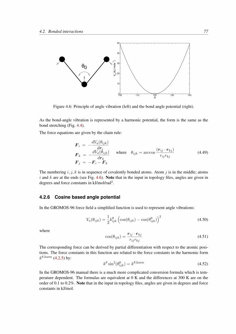
4.2. Bonded interactions 77
θ0
100 110 120 130 140θ
0
10
20
30
40
50
Vθ (
kJ m
ole
-1)
Figure 4.6: Principle of angle vibration (left) and the bond angle potential (right).
As the bond-angle vibration is represented by a harmonic potential, the form is the same as thebond stretching (Fig. 4.4).
The force equations are given by the chain rule:
F i = −dVa(θijk)dri
F k = −dVa(θijk)drk
F j = −F i − F k
where θijk = arccos(rij · rkj)rijrkj
(4.49)
The numbering i, j, k is in sequence of covalently bonded atoms. Atom j is in the middle; atomsi and k are at the ends (see Fig. 4.6). Note that in the input in topology files, angles are given indegrees and force constants in kJ/mol/rad2.
4.2.6 Cosine based angle potential
In the GROMOS-96 force field a simplified function is used to represent angle vibrations:
Va(θijk) =1
2kθijk
(cos(θijk)− cos(θ0
ijk))2
(4.50)
wherecos(θijk) =
rij · rkjrijrkj
(4.51)
The corresponding force can be derived by partial differentiation with respect to the atomic posi-tions. The force constants in this function are related to the force constants in the harmonic formkθ,harm (4.2.5) by:
kθ sin2(θ0ijk) = kθ,harm (4.52)
In the GROMOS-96 manual there is a much more complicated conversion formula which is tem-perature dependent. The formulas are equivalent at 0 K and the differences at 300 K are on theorder of 0.1 to 0.2%. Note that in the input in topology files, angles are given in degrees and forceconstants in kJ/mol.

78 Chapter 4. Interaction function and force fields
Figure 4.7: Bending angle potentials: cosine harmonic (solid black line), angle harmonic (dashedblack line) and restricted bending (red) with the same bending constant kθ = 85 kJ mol−1 andequilibrium angle θ0 = 130. The orange line represents the sum of a cosine harmonic (k = 50kJ mol−1) with a restricted bending (k = 25 kJ mol−1) potential, both with θ0 = 130.
4.2.7 Restricted bending potential
The restricted bending (ReB) potential [88] prevents the bending angle θ from reaching the 180
value. In this way, the numerical instabilities due to the calculation of the torsion angle andpotential are eliminated when performing coarse-grained molecular dynamics simulations.
To systematically hinder the bending angles from reaching the 180 value, the bending potential4.50 is divided by a sin2 θ factor:
VReB(θi) =1
2kθ
(cos θi − cos θ0)2
sin2 θi. (4.53)
Figure Fig. 4.7 shows the comparison between the ReB potential, 4.53, and the standard one 4.50.The wall of the ReB potential is very repulsive in the region close to 180 and, as a result, thebending angles are kept within a safe interval, far from instabilities. The power 2 of sin θi in thedenominator has been chosen to guarantee this behavior and allows an elegant differentiation:
FReB(θi) =2kθ
sin4 θi(cos θi − cos θ0)(1− cos θi cos θ0)
∂ cos θi∂~rk
. (4.54)
Due to its construction, the restricted bending potential cannot be used for equilibrium θ0 valuestoo close to 0 or 180 (from experience, at least 10 difference is recommended). It is veryimportant that, in the starting configuration, all the bending angles have to be in the safe intervalto avoid initial instabilities. This bending potential can be used in combination with any formof torsion potential. It will always prevent three consecutive particles from becoming collinearand, as a result, any torsion potential will remain free of singularities. It can be also added to a

4.2. Bonded interactions 79
standard bending potential to affect the angle around 180, but to keep its original form around theminimum (see the orange curve in Fig. 4.7).
4.2.8 Urey-Bradley potential
The Urey-Bradley bond-angle vibration between a triplet of atoms i - j - k is represented by aharmonic potential on the angle θijk and a harmonic correction term on the distance between theatoms i and k. Although this can be easily written as a simple sum of two terms, it is convenientto have it as a single entry in the topology file and in the output as a separate energy term. It isused mainly in the CHARMm force field [89]. The energy is given by:
Va(θijk) =1
2kθijk(θijk − θ0
ijk)2 +
1
2kUBijk (rik − r0
ik)2 (4.55)
The force equations can be deduced from sections 4.2.1 and 4.2.5.
4.2.9 Bond-Bond cross term
The bond-bond cross term for three particles i, j, k forming bonds i− j and k− j is given by [90]:
Vrr′ = krr′ (|ri − rj | − r1e) (|rk − rj | − r2e) (4.56)
where krr′ is the force constant, and r1e and r2e are the equilibrium bond lengths of the i− j andk − j bonds respectively. The force associated with this potential on particle i is:
F i = −krr′ (|rk − rj | − r2e)ri − rj|ri − rj |
(4.57)
The force on atom k can be obtained by swapping i and k in the above equation. Finally, the forceon atom j follows from the fact that the sum of internal forces should be zero: F j = −F i − F k.
4.2.10 Bond-Angle cross term
The bond-angle cross term for three particles i, j, k forming bonds i−j and k−j is given by [90]:
Vrθ = krθ (|ri − rk| − r3e) (|ri − rj | − r1e + |rk − rj | − r2e) (4.58)
where krθ is the force constant, r3e is the i − k distance, and the other constants are the same asin Equation 4.56. The force associated with the potential on atom i is:
F i = −krθ
[(|ri − rk| − r3e)
ri − rj|ri − rj |
+ (|ri − rj | − r1e + |rk − rj | − r2e)ri − rk|ri − rk|
](4.59)
4.2.11 Quartic angle potential
For special purposes there is an angle potential that uses a fourth order polynomial:
Vq(θijk) =5∑
n=0
Cn(θijk − θ0ijk)
n (4.60)

80 Chapter 4. Interaction function and force fields
k
li
ji
kj
l
k
i
j
l
Figure 4.8: Principle of improper dihedral angles. Out of plane bending for rings (left), sub-stituents of rings (middle), out of tetrahedral (right). The improper dihedral angle ξ is defined asthe angle between planes (i,j,k) and (j,k,l) in all cases.
–20 –10 0 10 20ξ
0
10
20
V i (k
J m
ol–1
)
(°)
Figure 4.9: Improper dihedral potential.
4.2.12 Improper dihedrals
Improper dihedrals are meant to keep planar groups (e.g. aromatic rings) planar, or to preventmolecules from flipping over to their mirror images, see Fig. 4.8.
Improper dihedrals: harmonic type
The simplest improper dihedral potential is a harmonic potential; it is plotted in Fig. 4.9.
Vid(ξijkl) =1
2kξ(ξijkl − ξ0)2 (4.61)
Since the potential is harmonic it is discontinuous, but since the discontinuity is chosen at 180
distance from ξ0 this will never cause problems. Note that in the input in topology files, angles aregiven in degrees and force constants in kJ/mol/rad2.

4.2. Bonded interactions 81
j
k
l
i0.0 90.0 180.0 270.0 360.0
φ
0.0
20.0
40.0
60.0
80.0
Vd
(kJ
mol
e–1)
Figure 4.10: Principle of proper dihedral angle (left, in trans form) and the dihedral angle potential(right).
Improper dihedrals: periodic type
This potential is identical to the periodic proper dihedral (see below). There is a separate dihedraltype for this (type 4) only to be able to distinguish improper from proper dihedrals in the parametersection and the output.
4.2.13 Proper dihedrals
For the normal dihedral interaction there is a choice of either the GROMOS periodic function or afunction based on expansion in powers of cosφ (the so-called Ryckaert-Bellemans potential). Thischoice has consequences for the inclusion of special interactions between the first and the fourthatom of the dihedral quadruple. With the periodic GROMOS potential a special 1-4 LJ-interactionmust be included; with the Ryckaert-Bellemans potential for alkanes the 1-4 interactions must beexcluded from the non-bonded list. Note: Ryckaert-Bellemans potentials are also used in e.g. theOPLS force field in combination with 1-4 interactions. You should therefore not modify topologiesgenerated by pdb2gmx in this case.
Proper dihedrals: periodic type
Proper dihedral angles are defined according to the IUPAC/IUB convention, where φ is the anglebetween the ijk and the jkl planes, with zero corresponding to the cis configuration (i and l onthe same side). There are two dihedral function types in GROMACS topology files. There is thestandard type 1 which behaves like any other bonded interactions. For certain force fields, type 9 isuseful. Type 9 allows multiple potential functions to be applied automatically to a single dihedralin the [ dihedral ] section when multiple parameters are defined for the same atomtypes inthe [ dihedraltypes ] section.
Vd(φijkl) = kφ(1 + cos(nφ− φs)) (4.62)

82 Chapter 4. Interaction function and force fields
C0 9.28 C2 -13.12 C4 26.24C1 12.16 C3 -3.06 C5 -31.5
Table 4.1: Constants for Ryckaert-Bellemans potential (kJ mol−1).
0.0 90.0 180.0 270.0 360.0φ
0.0
10.0
20.0
30.0
40.0
50.0
Vd
(kJ
mol
e–1)
Figure 4.11: Ryckaert-Bellemans dihedral potential.
Proper dihedrals: Ryckaert-Bellemans function
For alkanes, the following proper dihedral potential is often used (see Fig. 4.11):
Vrb(φijkl) =5∑
n=0
Cn(cos(ψ))n, (4.63)
where ψ = φ− 180.Note: A conversion from one convention to another can be achieved by multiplying every coeffi-cient Cn by (−1)n.
An example of constants for C is given in Table 4.1.
(Note: The use of this potential implies exclusion of LJ interactions between the first and the lastatom of the dihedral, and ψ is defined according to the “polymer convention” (ψtrans = 0).)
The RB dihedral function can also be used to include Fourier dihedrals (see below):
Vrb(φijkl) =1
2[F1(1 + cos(φ)) + F2(1− cos(2φ)) + F3(1 + cos(3φ)) + F4(1− cos(4φ))]
(4.64)Because of the equalities cos(2φ) = 2 cos2(φ)−1, cos(3φ) = 4 cos3(φ)−3 cos(φ) and cos(4φ) =8 cos4(φ)− 8 cos2(φ) + 1 one can translate the OPLS parameters to Ryckaert-Bellemans param-

4.2. Bonded interactions 83
eters as follows:C0 = F2 + 1
2(F1 + F3)C1 = 1
2(−F1 + 3F3)C2 = −F2 + 4F4
C3 = −2F3
C4 = −4F4
C5 = 0
(4.65)
with OPLS parameters in protein convention and RB parameters in polymer convention (this yieldsa minus sign for the odd powers of cos(φ)).Note: Mind the conversion from kcal mol−1 for literature OPLS and RB parameters to kJ mol−1
in GROMACS.
Proper dihedrals: Fourier function
The OPLS potential function is given as the first three [91] or four [92] cosine terms of a Fourierseries. In GROMACS the four term function is implemented:
VF (φijkl) =1
2[C1(1 + cos(φ)) + C2(1− cos(2φ)) + C3(1 + cos(3φ)) + C4(1− cos(4φ))] ,
(4.66)Internally, GROMACS uses the Ryckaert-Bellemans code to compute Fourier dihedrals (see above),because this is more efficient.Note: Mind the conversion from kcal mol−1 for literature OPLS parameters to kJ mol−1 in GRO-MACS.
Proper dihedrals: Restricted torsion potential
In a manner very similar to the restricted bending potential (see 4.2.7), a restricted torsion/dihedralpotential is introduced:
VReT(φi) =1
2kφ
(cosφi − cosφ0)2
sin2 φi(4.67)
with the advantages of being a function of cosφ (no problems taking the derivative of sinφ) andof keeping the torsion angle at only one minimum value. In this case, the factor sin2 φ does notallow the dihedral angle to move from the [−180:0] to [0:180] interval, i.e. it cannot havemaxima both at −φ0 and +φ0 maxima, but only one of them. For this reason, all the dihedralangles of the starting configuration should have their values in the desired angles interval and thethe equilibrium φ0 value should not be too close to the interval limits (as for the restricted bendingpotential, described in 4.2.7, at least 10 difference is recommended).
Proper dihedrals: Combined bending-torsion potential
When the four particles forming the dihedral angle become collinear (this situation will neverhappen in atomistic simulations, but it can occur in coarse-grained simulations) the calculation of

84 Chapter 4. Interaction function and force fields
the torsion angle and potential leads to numerical instabilities. One way to avoid this is to use therestricted bending potential (see 4.2.7) that prevents the dihedral from reaching the 180 value.
Another way is to disregard any effects of the dihedral becoming ill-defined, keeping the dihedralforce and potential calculation continuous in entire angle range by coupling the torsion potential(in a cosine form) with the bending potentials of the adjacent bending angles in a unique expres-sion:
VCBT(θi−1, θi, φi) = kφ sin3 θi−1 sin3 θi
4∑n=0
an cosn φi. (4.68)
This combined bending-torsion (CBT) potential has been proposed by [93] for polymer melt sim-ulations and is extensively described in [88].
This potential has two main advantages:
• it does not only depend on the dihedral angle φi (between the i − 2, i − 1, i and i + 1beads) but also on the bending angles θi−1 and θi defined from three adjacent beads (i− 2,i − 1 and i, and i − 1, i and i + 1, respectively). The two sin3 θ pre-factors, tentativelysuggested by [94] and theoretically discussed by [95], cancel the torsion potential and forcewhen either of the two bending angles approaches the value of 180.
• its dependence on φi is expressed through a polynomial in cosφi that avoids the singularitiesin φ = 0 or 180 in calculating the torsional force.
These two properties make the CBT potential well-behaved for MD simulations with weak con-straints on the bending angles or even for steered / non-equilibrium MD in which the bending andtorsion angles suffer major modifications. When using the CBT potential, the bending potentialsfor the adjacent θi−1 and θi may have any form. It is also possible to leave out the two anglebending terms (θi−1 and θi) completely. Fig. 4.12 illustrates the difference between a torsion po-tential with and without the sin3 θ factors (blue and gray curves, respectively). Additionally, thederivative of VCBT with respect to the Cartesian variables is straightforward:
∂VCBT(θi−1, θi, φi)
∂~rl=∂VCBT
∂θi−1
∂θi−1
∂~rl+∂VCBT
∂θi
∂θi∂~rl
+∂VCBT
∂φi
∂φi∂~rl
(4.69)
The CBT is based on a cosine form without multiplicity, so it can only be symmetrical around 0.To obtain an asymmetrical dihedral angle distribution (e.g. only one maximum in [−180:180]interval), a standard torsion potential such as harmonic angle or periodic cosine potentials shouldbe used instead of a CBT potential. However, these two forms have the inconveniences of theforce derivation (1/ sinφ) and of the alignment of beads (θi or θi−1 = 0, 180). Coupling suchnon-cosφ potentials with sin3 θ factors does not improve simulation stability since there are casesin which θ and φ are simultaneously 180. The integration at this step would be possible (due tothe cancelling of the torsion potential) but the next step would be singular (θ is not 180 and φ isvery close to 180).
4.2.14 Tabulated bonded interaction functions
For full flexibility, any functional shape can be used for bonds, angles and dihedrals through user-supplied tabulated functions. The functional shapes are:
Vb(rij) = k f bn(rij) (4.70)

4.2. Bonded interactions 85
-180-90
090
180
030
6090
120150
180 0
5
10
15
20
25
30
35
40
45
VT [k
J m
ol-1
]
CBTRB
φ [deg]
θ [deg]
VT [k
J m
ol-1
]
Figure 4.12: Blue: surface plot of the combined bending-torsion potential (4.68 with k = 10kJ mol−1, a0 = 2.41, a1 = −2.95, a2 = 0.36, a3 = 1.33) when, for simplicity, the bendingangles behave the same (θ1 = θ2 = θ). Gray: the same torsion potential without the sin3 θ terms(Ryckaert-Bellemans type). φ is the dihedral angle.
Va(θijk) = k fan(θijk) (4.71)
Vd(φijkl) = k fdn(φijkl) (4.72)
where k is a force constant in units of energy and f is a cubic spline function; for details see 6.12.1.For each interaction, the force constant k and the table number n are specified in the topology.There are two different types of bonds, one that generates exclusions (type 8) and one that doesnot (type 9). For details see Table 5.5. The table files are supplied to the mdrun program. Afterthe table file name an underscore, the letter “b” for bonds, “a” for angles or “d” for dihedrals andthe table number must be appended. For example, a tabulated bond with n = 0 can be read fromthe file table_b0.xvg. Multiple tables can be supplied simply by adding files with differentvalues of n, and are applied to the appropriate bonds, as specified in the topology (Table 5.5).The format for the table files is three fixed-format columns of any suitable width. These columnsmust contain x, f(x), −f ′(x), and the values of x should be uniformly spaced. Requirements forentries in the topology are given in Table 5.5. The setup of the tables is as follows:bonds: x is the distance in nm. For distances beyond the table length, mdrun will quit with anerror message.angles: x is the angle in degrees. The table should go from 0 up to and including 180 degrees; thederivative is taken in degrees.dihedrals: x is the dihedral angle in degrees. The table should go from -180 up to and including180 degrees; the IUPAC/IUB convention is used, i.e. zero is cis, the derivative is taken in degrees.

86 Chapter 4. Interaction function and force fields
0.00 0.02 0.04 0.06 0.08 0.10r-R (nm)
0.0
2.0
4.0
6.0
8.0
10.0
Vpo
sre
(kJ
mol
e–1)
Figure 4.13: Position restraint potential.
4.3 Restraints
Special potentials are used for imposing restraints on the motion of the system, either to avoiddisastrous deviations, or to include knowledge from experimental data. In either case they are notreally part of the force field and the reliability of the parameters is not important. The potentialforms, as implemented in GROMACS, are mentioned just for the sake of completeness. Restraintsand constraints refer to quite different algorithms in GROMACS.
4.3.1 Position restraints
These are used to restrain particles to fixed reference positions Ri. They can be used duringequilibration in order to avoid drastic rearrangements of critical parts (e.g. to restrain motion in aprotein that is subjected to large solvent forces when the solvent is not yet equilibrated). Anotherapplication is the restraining of particles in a shell around a region that is simulated in detail, whilethe shell is only approximated because it lacks proper interaction from missing particles outsidethe shell. Restraining will then maintain the integrity of the inner part. For spherical shells, it is awise procedure to make the force constant depend on the radius, increasing from zero at the innerboundary to a large value at the outer boundary. This feature has not, however, been implementedin GROMACS.
The following form is used:
Vpr(ri) =1
2kpr|ri −Ri|2 (4.73)
The potential is plotted in Fig. 4.13.
The potential form can be rewritten without loss of generality as:
Vpr(ri) =1
2
[kxpr(xi −Xi)
2 x + kypr(yi − Yi)2 y + kzpr(zi − Zi)2 z]
(4.74)

4.3. Restraints 87
-1 -0.5 0 0.5 1
r [nm]
0
10
20
30
40
50
V(r
) [k
J/m
ol]
-1 -0.5 0 0.5 1
r [nm]
0
10
20
30
40
50
2 rfb
A B
Figure 4.14: Flat-bottomed position restraint potential. (A) Not inverted, (B) inverted.
Now the forces are:F xi = −kxpr (xi −Xi)
F yi = −kypr (yi − Yi)F zi = −kzpr (zi − Zi)
(4.75)
Using three different force constants the position restraints can be turned on or off in each spatialdimension; this means that atoms can be harmonically restrained to a plane or a line. Positionrestraints are applied to a special fixed list of atoms. Such a list is usually generated by thepdb2gmx program.
4.3.2 Flat-bottomed position restraints
Flat-bottomed position restraints can be used to restrain particles to part of the simulation volume.No force acts on the restrained particle within the flat-bottomed region of the potential, however aharmonic force acts to move the particle to the flat-bottomed region if it is outside it. It is possibleto apply normal and flat-bottomed position restraints on the same particle (however, only with thesame reference positionRi). The following general potential is used (Figure 4.14A):
Vfb(ri) =1
2kfb[dg(ri;Ri)− rfb]2H[dg(ri;Ri)− rfb], (4.76)
where Ri is the reference position, rfb is the distance from the center with a flat potential, kfb theforce constant, and H is the Heaviside step function. The distance dg(ri;Ri) from the referenceposition depends on the geometry g of the flat-bottomed potential.
The following geometries for the flat-bottomed potential are supported:Sphere (g = 1): The particle is kept in a sphere of given radius. The force acts towards the centerof the sphere. The following distance calculation is used:
dg(ri;Ri) = |ri −Ri| (4.77)
Cylinder (g = 6, 7, 8): The particle is kept in a cylinder of given radius parallel to the x (g = 6),y (g = 7), or z-axis (g = 8). For backwards compatibility, setting g = 2 is mapped to g = 8 in thecode so that old .tpr files and topologies work. The force from the flat-bottomed potential actstowards the axis of the cylinder. The component of the force parallel to the cylinder axis is zero.For a cylinder aligned along the z-axis:
dg(ri;Ri) =√
(xi −Xi)2 + (yi − Yi)2 (4.78)

88 Chapter 4. Interaction function and force fields
Layer (g = 3, 4, 5): The particle is kept in a layer defined by the thickness and the normal of thelayer. The layer normal can be parallel to the x, y, or z-axis. The force acts parallel to the layernormal.
dg(ri;Ri) = |xi −Xi|, or dg(ri;Ri) = |yi − Yi|, or dg(ri;Ri) = |zi − Zi|. (4.79)
It is possible to apply multiple independent flat-bottomed position restraints of different geometryon one particle. For example, applying a cylinder and a layer in z keeps a particle within a disk.Applying three layers in x, y, and z keeps the particle within a cuboid.
In addition, it is possible to invert the restrained region with the unrestrained region, leading toa potential that acts to keep the particle outside of the volume defined by Ri, g, and rfb. Thatfeature is switched on by defining a negative rfb in the topology. The following potential is used(Figure 4.14B):
V invfb (ri) =
1
2kfb[dg(ri;Ri)− |rfb|]2H[−(dg(ri;Ri)− |rfb|)]. (4.80)
4.3.3 Angle restraints
These are used to restrain the angle between two pairs of particles or between one pair of particlesand the z-axis. The functional form is similar to that of a proper dihedral. For two pairs of atoms:
Var(ri, rj , rk, rl) = kar(1− cos(n(θ − θ0))), where θ = arccos
(rj − ri‖rj − ri‖
· rl − rk‖rl − rk‖
)(4.81)
For one pair of atoms and the z-axis:
Var(ri, rj) = kar(1− cos(n(θ − θ0))), where θ = arccos
rj − ri‖rj − ri‖
·
001
(4.82)
A multiplicity (n) of 2 is useful when you do not want to distinguish between parallel and anti-parallel vectors. The equilibrium angle θ should be between 0 and 180 degrees for multiplicity 1and between 0 and 90 degrees for multiplicity 2.
4.3.4 Dihedral restraints
These are used to restrain the dihedral angle φ defined by four particles as in an improper dihedral(sec. 4.2.12) but with a slightly modified potential. Using:
φ′ = (φ− φ0) MOD 2π (4.83)
where φ0 is the reference angle, the potential is defined as:
Vdihr(φ′) =
12kdihr(φ
′ − φ0 −∆φ)2 for φ′ > ∆φ
0 for φ′ ≤ ∆φ(4.84)
where ∆φ is a user defined angle and kdihr is the force constant. Note that in the input in topologyfiles, angles are given in degrees and force constants in kJ/mol/rad2.

4.3. Restraints 89
0 0.1 0.2 0.3 0.4 0.5
r (nm)
0
5
10
15
Vdis
re (
kJ m
ol−
1)
r0
r1
r2
Figure 4.15: Distance Restraint potential.
4.3.5 Distance restraints
Distance restraints add a penalty to the potential when the distance between specified pairs ofatoms exceeds a threshold value. They are normally used to impose experimental restraints from,for instance, experiments in nuclear magnetic resonance (NMR), on the motion of the system.Thus, MD can be used for structure refinement using NMR data. In GROMACS there are threeways to impose restraints on pairs of atoms:
• Simple harmonic restraints: use [ bonds ] type 6 (see sec. 5.4.4).
• Piecewise linear/harmonic restraints: [ bonds ] type 10.
• Complex NMR distance restraints, optionally with pair, time and/or ensemble averaging.
The last two options will be detailed now.
The potential form for distance restraints is quadratic below a specified lower bound and betweentwo specified upper bounds, and linear beyond the largest bound (see Fig. 4.15).
Vdr(rij) =
12kdr(rij − r0)2 for rij < r0
0 for r0 ≤ rij < r1
12kdr(rij − r1)2 for r1 ≤ rij < r2
12kdr(r2 − r1)(2rij − r2 − r1) for r2 ≤ rij
(4.85)
The forces are
F i =
−kdr(rij − r0)rijrij
for rij < r0
0 for r0 ≤ rij < r1
−kdr(rij − r1)rijrij
for r1 ≤ rij < r2
−kdr(r2 − r1)rijrij
for r2 ≤ rij
(4.86)

90 Chapter 4. Interaction function and force fields
For restraints not derived from NMR data, this functionality will usually suffice and a section of[ bonds ] type 10 can be used to apply individual restraints between pairs of atoms, see 5.8.1.For applying restraints derived from NMR measurements, more complex functionality might be re-quired, which is provided through the [ distance_restraints ] section and is describedbelow.
Time averaging
Distance restraints based on instantaneous distances can potentially reduce the fluctuations in amolecule significantly. This problem can be overcome by restraining to a time averaged dis-tance [96]. The forces with time averaging are:
F i =
−kadr(rij − r0)rijrij
for rij < r0
0 for r0 ≤ rij < r1
−kadr(rij − r1)rijrij
for r1 ≤ rij < r2
−kadr(r2 − r1)rijrij
for r2 ≤ rij
(4.87)
where rij is given by an exponential running average with decay time τ :
rij = < r−3ij >−1/3 (4.88)
The force constant kadr is switched on slowly to compensate for the lack of history at the beginningof the simulation:
kadr = kdr
(1− exp
(− tτ
))(4.89)
Because of the time averaging, we can no longer speak of a distance restraint potential.
This way an atom can satisfy two incompatible distance restraints on average by moving betweentwo positions. An example would be an amino acid side-chain that is rotating around its χ dihedralangle, thereby coming close to various other groups. Such a mobile side chain can give rise tomultiple NOEs that can not be fulfilled by a single structure.
The computation of the time averaged distance in the mdrun program is done in the followingfashion:
r−3ij(0) = rij(0)−3
r−3ij(t) = r−3
ij(t−∆t) exp(−∆t
τ
)+ rij(t)
−3[1− exp
(−∆t
τ
)] (4.90)
When a pair is within the bounds, it can still feel a force because the time averaged distance canstill be beyond a bound. To prevent the protons from being pulled too close together, a mixedapproach can be used. In this approach, the penalty is zero when the instantaneous distance iswithin the bounds, otherwise the violation is the square root of the product of the instantaneousviolation and the time averaged violation:
F i =
kadr
√(rij − r0)(rij − r0)
rijrij
for rij < r0 and rij < r0
−kadr min(√
(rij − r1)(rij − r1), r2 − r1
)rijrij
for rij > r1 and rij > r1
0 otherwise(4.91)

4.3. Restraints 91
Averaging over multiple pairs
Sometimes it is unclear from experimental data which atom pair gives rise to a single NOE, inother occasions it can be obvious that more than one pair contributes due to the symmetry of thesystem, e.g. a methyl group with three protons. For such a group, it is not possible to distinguishbetween the protons, therefore they should all be taken into account when calculating the distancebetween this methyl group and another proton (or group of protons). Due to the physical nature ofmagnetic resonance, the intensity of the NOE signal is inversely proportional to the sixth powerof the inter-atomic distance. Thus, when combining atom pairs, a fixed list of N restraints may betaken together, where the apparent “distance” is given by:
rN (t) =
[N∑n=1
rn(t)−6
]−1/6
(4.92)
where we use rij or eqn. 4.88 for the rn. The rN of the instantaneous and time-averaged distancescan be combined to do a mixed restraining, as indicated above. As more pairs of protons contributeto the same NOE signal, the intensity will increase, and the summed “distance” will be shorter thanany of its components due to the reciprocal summation.
There are two options for distributing the forces over the atom pairs. In the conservative option,the force is defined as the derivative of the restraint potential with respect to the coordinates. Thisresults in a conservative potential when time averaging is not used. The force distribution overthe pairs is proportional to r−6. This means that a close pair feels a much larger force than adistant pair, which might lead to a molecule that is “too rigid.” The other option is an equalforce distribution. In this case each pair feels 1/N of the derivative of the restraint potential withrespect to rN . The advantage of this method is that more conformations might be sampled, but thenon-conservative nature of the forces can lead to local heating of the protons.
It is also possible to use ensemble averaging using multiple (protein) molecules. In this case thebounds should be lowered as in:
r1 = r1 ∗M−1/6
r2 = r2 ∗M−1/6 (4.93)
where M is the number of molecules. The GROMACS preprocessor grompp can do this auto-matically when the appropriate option is given. The resulting “distance” is then used to calculatethe scalar force according to:
F i =
0 rN < r1
kdr(rN − r1)rijrij
r1 ≤ rN < r2
kdr(r2 − r1)rijrij
rN ≥ r2
(4.94)
where i and j denote the atoms of all the pairs that contribute to the NOE signal.
Using distance restraints
A list of distance restrains based on NOE data can be added to a molecule definition in yourtopology file, like in the following example:

92 Chapter 4. Interaction function and force fields
[ distance_restraints ]; ai aj type index type’ low up1 up2 fac10 16 1 0 1 0.0 0.3 0.4 1.010 28 1 1 1 0.0 0.3 0.4 1.010 46 1 1 1 0.0 0.3 0.4 1.016 22 1 2 1 0.0 0.3 0.4 2.516 34 1 3 1 0.0 0.5 0.6 1.0
In this example a number of features can be found. In columns ai and aj you find the atomnumbers of the particles to be restrained. The type column should always be 1. As explainedin 4.3.5, multiple distances can contribute to a single NOE signal. In the topology this can beset using the index column. In our example, the restraints 10-28 and 10-46 both have index 1,therefore they are treated simultaneously. An extra requirement for treating restraints together isthat the restraints must be on successive lines, without any other intervening restraint. The type’column will usually be 1, but can be set to 2 to obtain a distance restraint that will never be time-and ensemble-averaged; this can be useful for restraining hydrogen bonds. The columns low,up1, and up2 hold the values of r0, r1, and r2 from eqn. 4.85. In some cases it can be usefulto have different force constants for some restraints; this is controlled by the column fac. Theforce constant in the parameter file is multiplied by the value in the column fac for each restraint.Information for each restraint is stored in the energy file and can be processed and plotted withgmx nmr.
4.3.6 Orientation restraints
This section describes how orientations between vectors, as measured in certain NMR experi-ments, can be calculated and restrained in MD simulations. The presented refinement methodol-ogy and a comparison of results with and without time and ensemble averaging have been pub-lished [97].
Theory
In an NMR experiment, orientations of vectors can be measured when a molecule does not tum-ble completely isotropically in the solvent. Two examples of such orientation measurements areresidual dipolar couplings (between two nuclei) or chemical shift anisotropies. An observable fora vector ri can be written as follows:
δi =2
3tr(SDi) (4.95)
where S is the dimensionless order tensor of the molecule. The tensor Di is given by:
Di =ci‖ri‖α
3xx− 1 3xy 3xz3xy 3yy − 1 3yz3xz 3yz 3zz − 1
(4.96)
with: x =ri,x‖ri‖
, y =ri,y‖ri‖
, z =ri,z‖ri‖
(4.97)
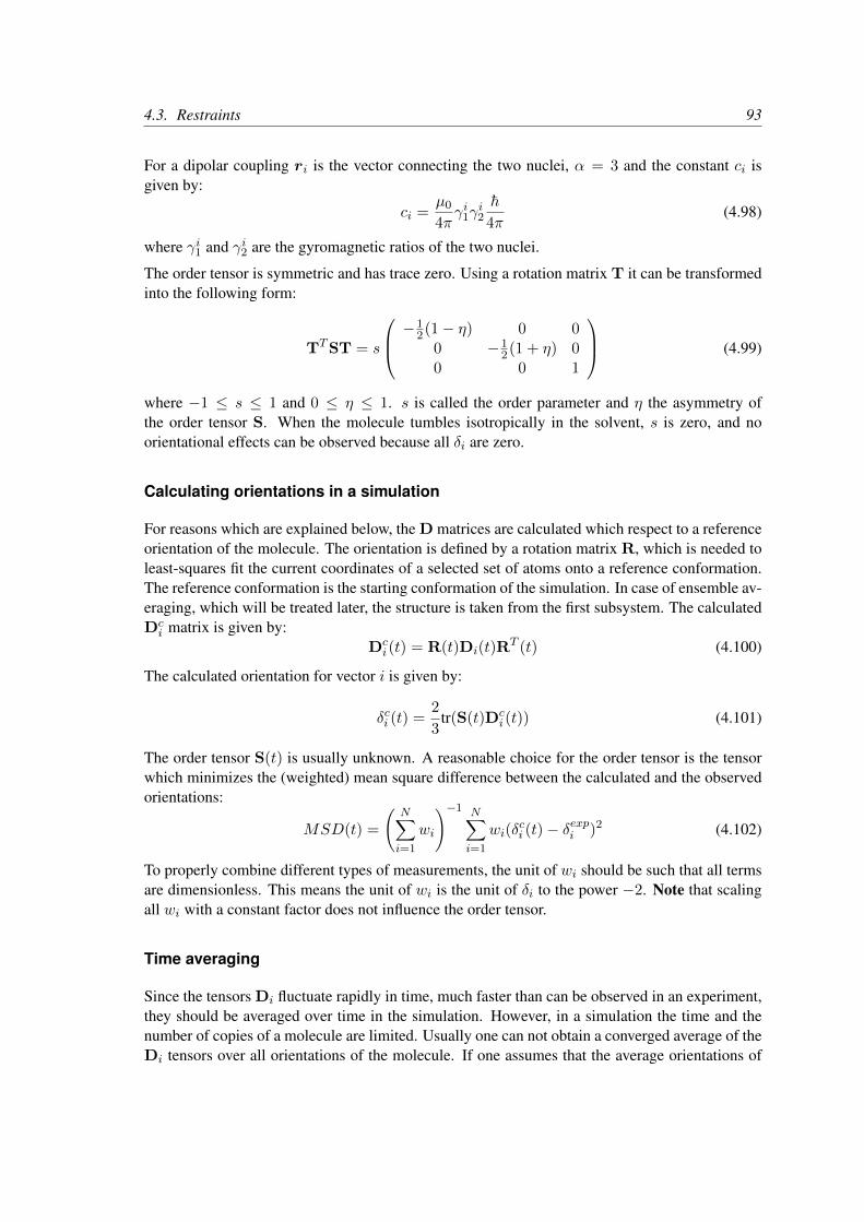
4.3. Restraints 93
For a dipolar coupling ri is the vector connecting the two nuclei, α = 3 and the constant ci isgiven by:
ci =µ0
4πγi1γ
i2
h
4π(4.98)
where γi1 and γi2 are the gyromagnetic ratios of the two nuclei.
The order tensor is symmetric and has trace zero. Using a rotation matrix T it can be transformedinto the following form:
TTST = s
−12(1− η) 0 0
0 −12(1 + η) 0
0 0 1
(4.99)
where −1 ≤ s ≤ 1 and 0 ≤ η ≤ 1. s is called the order parameter and η the asymmetry ofthe order tensor S. When the molecule tumbles isotropically in the solvent, s is zero, and noorientational effects can be observed because all δi are zero.
Calculating orientations in a simulation
For reasons which are explained below, the D matrices are calculated which respect to a referenceorientation of the molecule. The orientation is defined by a rotation matrix R, which is needed toleast-squares fit the current coordinates of a selected set of atoms onto a reference conformation.The reference conformation is the starting conformation of the simulation. In case of ensemble av-eraging, which will be treated later, the structure is taken from the first subsystem. The calculatedDci matrix is given by:
Dci (t) = R(t)Di(t)R
T (t) (4.100)
The calculated orientation for vector i is given by:
δci (t) =2
3tr(S(t)Dc
i (t)) (4.101)
The order tensor S(t) is usually unknown. A reasonable choice for the order tensor is the tensorwhich minimizes the (weighted) mean square difference between the calculated and the observedorientations:
MSD(t) =
(N∑i=1
wi
)−1 N∑i=1
wi(δci (t)− δ
expi )2 (4.102)
To properly combine different types of measurements, the unit of wi should be such that all termsare dimensionless. This means the unit of wi is the unit of δi to the power −2. Note that scalingall wi with a constant factor does not influence the order tensor.
Time averaging
Since the tensors Di fluctuate rapidly in time, much faster than can be observed in an experiment,they should be averaged over time in the simulation. However, in a simulation the time and thenumber of copies of a molecule are limited. Usually one can not obtain a converged average of theDi tensors over all orientations of the molecule. If one assumes that the average orientations of

94 Chapter 4. Interaction function and force fields
the ri vectors within the molecule converge much faster than the tumbling time of the molecule,the tensor can be averaged in an axis system that rotates with the molecule, as expressed by equa-tion (4.100). The time-averaged tensors are calculated using an exponentially decaying memoryfunction:
Dai (t) =
∫ t
u=t0Dci (u) exp
(− t− u
τ
)du∫ t
u=t0exp
(− t− u
τ
)du
(4.103)
Assuming that the order tensor S fluctuates slower than the Di, the time-averaged orientation canbe calculated as:
δai (t) =2
3tr(S(t)Da
i (t)) (4.104)
where the order tensor S(t) is calculated using expression (4.102) with δci (t) replaced by δai (t).
Restraining
The simulated structure can be restrained by applying a force proportional to the difference be-tween the calculated and the experimental orientations. When no time averaging is applied, aproper potential can be defined as:
V =1
2k
N∑i=1
wi(δci (t)− δ
expi )2 (4.105)
where the unit of k is the unit of energy. Thus the effective force constant for restraint i is kwi.The forces are given by minus the gradient of V . The force Fi working on vector ri is:
Fi(t) = −dVdri
= −kwi(δci (t)− δexpi )
dδi(t)dri
= −kwi(δci (t)− δexpi )
2ci‖r‖2+α
(2RTSRri −
2 + α
‖r‖2tr(RTSRrir
Ti )ri
)
Ensemble averaging
Ensemble averaging can be applied by simulating a system of M subsystems that each containan identical set of orientation restraints. The systems only interact via the orientation restraintpotential which is defined as:
V = M1
2k
N∑i=1
wi〈δci (t)− δexpi 〉
2 (4.106)
The force on vector ri,m in subsystem m is given by:
Fi,m(t) = − dVdri,m
= −kwi〈δci (t)− δexpi 〉
dδci,m(t)
dri,m(4.107)

4.3. Restraints 95
Time averaging
When using time averaging it is not possible to define a potential. We can still define a quantitythat gives a rough idea of the energy stored in the restraints:
V = M1
2ka
N∑i=1
wi〈δai (t)− δexpi 〉2 (4.108)
The force constant ka is switched on slowly to compensate for the lack of history at times close tot0. It is exactly proportional to the amount of average that has been accumulated:
ka = k1
τ
∫ t
u=t0exp
(− t− u
τ
)du (4.109)
What really matters is the definition of the force. It is chosen to be proportional to the square rootof the product of the time-averaged and the instantaneous deviation. Using only the time-averageddeviation induces large oscillations. The force is given by:
Fi,m(t) =
0 for a b ≤ 0
kawia
|a|√a b
dδci,m(t)
dri,mfor a b > 0
(4.110)
a = 〈δai (t)− δexpi 〉b = 〈δci (t)− δ
expi 〉
Using orientation restraints
Orientation restraints can be added to a molecule definition in the topology file in the section[ orientation_restraints ]. Here we give an example section containing five N-Hresidual dipolar coupling restraints:
[ orientation_restraints ]; ai aj type exp. label alpha const. obs. weight; Hz nm^3 Hz Hz^-2
31 32 1 1 3 3 6.083 -6.73 1.043 44 1 1 4 3 6.083 -7.87 1.055 56 1 1 5 3 6.083 -7.13 1.065 66 1 1 6 3 6.083 -2.57 1.073 74 1 1 7 3 6.083 -2.10 1.0
The unit of the observable is Hz, but one can choose any other unit. In columns ai and aj youfind the atom numbers of the particles to be restrained. The type column should always be 1. Theexp. column denotes the experiment number, starting at 1. For each experiment a separate ordertensor S is optimized. The label should be a unique number larger than zero for each restraint. Thealpha column contains the power α that is used in equation (4.96) to calculate the orientation.The const. column contains the constant ci used in the same equation. The constant should

96 Chapter 4. Interaction function and force fields
have the unit of the observable times nmα. The column obs. contains the observable, in any unityou like. The last column contains the weights wi; the unit should be the inverse of the square ofthe unit of the observable.
Some parameters for orientation restraints can be specified in the grompp.mdp file, for a studyof the effect of different force constants and averaging times and ensemble averaging see [97].Information for each restraint is stored in the energy file and can be processed and plotted withgmx nmr.
4.4 Polarization
Polarization can be treated by GROMACS by attaching shell (Drude) particles to atoms and/orvirtual sites. The energy of the shell particle is then minimized at each time step in order to remainon the Born-Oppenheimer surface.
4.4.1 Simple polarization
This is implemented as a harmonic potential with equilibrium distance 0. The input given in thetopology file is the polarizability α (in GROMACS units) as follows:
[ polarization ]; Atom i j type alpha1 2 1 0.001
in this case the polarizability volume is 0.001 nm3 (or 1 Å3). In order to compute the harmonicforce constant kcs (where cs stands for core-shell), the following is used [45]:
kcs =q2s
α(4.111)
where qs is the charge on the shell particle.
4.4.2 Anharmonic polarization
For the development of the Drude force field by Roux and McKerell [98] it was found that someparticles can overpolarize and this was fixed by introducing a higher order term in the polarizationenergy:
Vpol = kcs2 r
2cs rcs ≤ δ (4.112)
= kcs2 r
2cs + khyp(rcs − δ)4 rcs > δ (4.113)
where δ is a user-defined constant that is set to 0.02 nm for anions in the Drude force field [99].Since this original introduction it has also been used in other atom types [98].
[ polarization ];Atom i j type alpha (nm^3) delta khyp1 2 2 0.001786 0.02 16.736e8
The above force constant khyp corresponds to 4·108 kcal/mol/nm4, hence the strange number.

4.5. Free energy interactions 97
4.4.3 Water polarization
A special potential for water that allows anisotropic polarization of a single shell particle [45].
4.4.4 Thole polarization
Based on early work by Thole [100], Roux and coworkers have implemented potentials for moleculeslike ethanol [101, 102, 103]. Within such molecules, there are intra-molecular interactions be-tween shell particles, however these must be screened because full Coulomb would be too strong.The potential between two shell particles i and j is:
Vthole =qiqjrij
[1−
(1 +
rij2
)exp−rij
](4.114)
Note that there is a sign error in Equation 1 of Noskov et al. [103]:
rij = arij
(αiαj)1/6(4.115)
where a is a magic (dimensionless) constant, usually chosen to be 2.6 [103]; αi and αj are thepolarizabilities of the respective shell particles.
4.5 Free energy interactions
This section describes the λ-dependence of the potentials used for free energy calculations (seesec. 3.12). All common types of potentials and constraints can be interpolated smoothly from stateA (λ = 0) to state B (λ = 1) and vice versa. All bonded interactions are interpolated by linearinterpolation of the interaction parameters. Non-bonded interactions can be interpolated linearlyor via soft-core interactions.
Starting in GROMACS 4.6, λ is a vector, allowing different components of the free energy trans-formation to be carried out at different rates. Coulomb, Lennard-Jones, bonded, and restraint termscan all be controlled independently, as described in the .mdp options.
Harmonic potentials
The example given here is for the bond potential, which is harmonic in GROMACS. However,these equations apply to the angle potential and the improper dihedral potential as well.
Vb =1
2
[(1− λ)kAb + λkBb
] [b− (1− λ)bA0 − λbB0
]2(4.116)
∂Vb∂λ
=1
2(kBb − kAb )
[b− (1− λ)bA0 + λbB0
]2+
(bA0 − bB0 )[b− (1− λ)bA0 − λbB0
] [(1− λ)kAb + λkBb
](4.117)
98 Chapter 4. Interaction function and force fields
GROMOS-96 bonds and angles
Fourth-power bond stretching and cosine-based angle potentials are interpolated by linear interpo-lation of the force constant and the equilibrium position. Formulas are not given here.
Proper dihedrals
For the proper dihedrals, the equations are somewhat more complicated:
Vd =[(1− λ)kAd + λkBd
] (1 + cos
[nφφ− (1− λ)φAs − λφBs
])(4.118)
∂Vd∂λ
= (kBd − kAd )(1 + cos
[nφφ− (1− λ)φAs − λφBs
])+
(φBs − φAs )[(1− λ)kAd − λkBd
]sin[nφφ− (1− λ)φAs − λφBs
](4.119)
Note: that the multiplicity nφ can not be parameterized because the function should remain peri-odic on the interval [0, 2π].
Tabulated bonded interactions
For tabulated bonded interactions only the force constant can interpolated:
V = ((1− λ)kA + λkB) f (4.120)∂V
∂λ= (kB − kA) f (4.121)
Coulomb interaction
The Coulomb interaction between two particles of which the charge varies with λ is:
Vc =f
εrfrij
[(1− λ)qAi q
Aj + λ qBi q
Bj
](4.122)
∂Vc∂λ
=f
εrfrij
[−qAi qAj + qBi q
Bj
](4.123)
where f = 14πε0
= 138.935 458 (see chapter 2).
Coulomb interaction with reaction field
The Coulomb interaction including a reaction field, between two particles of which the chargevaries with λ is:
Vc = f
[1
rij+ krf r
2ij − crf
] [(1− λ)qAi q
Aj + λ qBi q
Bj
](4.124)
∂Vc∂λ
= f
[1
rij+ krf r
2ij − crf
] [−qAi qAj + qBi q
Bj
](4.125)
Note that the constants krf and crf are defined using the dielectric constant εrf of the medium(see sec. 4.1.4).

4.5. Free energy interactions 99
Lennard-Jones interaction
For the Lennard-Jones interaction between two particles of which the atom type varies with λ wecan write:
VLJ =(1− λ)CA12 + λCB12
r12ij
− (1− λ)CA6 + λCB6r6ij
(4.126)
∂VLJ∂λ
=CB12 − CA12
r12ij
− CB6 − CA6r6ij
(4.127)
It should be noted that it is also possible to express a pathway from state A to state B using σ andε (see eqn. 4.5). It may seem to make sense physically to vary the force field parameters σ and εrather than the derived parameters C12 and C6. However, the difference between the pathways inparameter space is not large, and the free energy itself does not depend on the pathway, so we usethe simple formulation presented above.
Kinetic Energy
When the mass of a particle changes, there is also a contribution of the kinetic energy to the freeenergy (note that we can not write the momentum p as mv, since that would result in the sign of∂Ek∂λ being incorrect [104]):
Ek =1
2
p2
(1− λ)mA + λmB(4.128)
∂Ek∂λ
= −1
2
p2(mB −mA)
((1− λ)mA + λmB)2(4.129)
after taking the derivative, we can insert p = mv, such that:
∂Ek∂λ
= −1
2v2(mB −mA) (4.130)
Constraints
The constraints are formally part of the Hamiltonian, and therefore they give a contribution to thefree energy. In GROMACS this can be calculated using the LINCS or the SHAKE algorithm. Ifwe have k = 1 . . .K constraint equations gk for LINCS, then
gk = |rk| − dk (4.131)
where rk is the displacement vector between two particles and dk is the constraint distance be-tween the two particles. We can express the fact that the constraint distance has a λ dependencyby
dk = (1− λ)dAk + λdBk (4.132)
Thus the λ-dependent constraint equation is
gk = |rk| −((1− λ)dAk + λdBk
). (4.133)

100 Chapter 4. Interaction function and force fields
0 0.5 1 1.5 2 2.5 3
r
−1
0
1
2
3
4
5
Vsc
LJ, α=0
LJ, α=1.5
LJ, α=2
3/r, α=0
3/r, α=1.5
3/r, α=2
Figure 4.16: Soft-core interactions at λ = 0.5, with p = 2 and CA6 = CA12 = CB6 = CB12 = 1.
The (zero) contribution G to the Hamiltonian from the constraints (using Lagrange multipliers λk,which are logically distinct from the free-energy λ) is
G =K∑k
λkgk (4.134)
∂G
∂λ=
∂G
∂dk
∂dk∂λ
(4.135)
= −K∑k
λk(dBk − dAk
)(4.136)
For SHAKE, the constraint equations are
gk = r2k − d2
k (4.137)
with dk as before, so
∂G
∂λ= −2
K∑k
λk(dBk − dAk
)(4.138)
4.5.1 Soft-core interactions
In a free-energy calculation where particles grow out of nothing, or particles disappear, using thethe simple linear interpolation of the Lennard-Jones and Coulomb potentials as described in Equa-tions 4.127 and 4.125 may lead to poor convergence. When the particles have nearly disappeared,or are close to appearing (at λ close to 0 or 1), the interaction energy will be weak enough forparticles to get very close to each other, leading to large fluctuations in the measured values of∂V/∂λ (which, because of the simple linear interpolation, depends on the potentials at both theendpoints of λ).

4.5. Free energy interactions 101
To circumvent these problems, the singularities in the potentials need to be removed. This can bedone by modifying the regular Lennard-Jones and Coulomb potentials with “soft-core” potentialsthat limit the energies and forces involved at λ values between 0 and 1, but not at λ = 0 or 1.
In GROMACS the soft-core potentials Vsc are shifted versions of the regular potentials, so that thesingularity in the potential and its derivatives at r = 0 is never reached:
Vsc(r) = (1− λ)V A(rA) + λV B(rB) (4.139)
rA =(ασ6
Aλp + r6
) 16 (4.140)
rB =(ασ6
B(1− λ)p + r6) 1
6 (4.141)
where V A and V B are the normal “hard core” Van der Waals or electrostatic potentials in state A(λ = 0) and state B (λ = 1) respectively, α is the soft-core parameter (set with sc_alpha inthe .mdp file), p is the soft-core λ power (set with sc_power), σ is the radius of the interaction,which is (C12/C6)1/6 or an input parameter (sc_sigma) when C6 or C12 is zero.
For intermediate λ, rA and rB alter the interactions very little for r > α1/6σ and quickly switchthe soft-core interaction to an almost constant value for smaller r (Fig. 4.16). The force is:
Fsc(r) = −∂Vsc(r)∂r
= (1− λ)FA(rA)
(r
rA
)5
+ λFB(rB)
(r
rB
)5
(4.142)
where FA and FB are the “hard core” forces. The contribution to the derivative of the free energyis:
∂Vsc(r)
∂λ= V B(rB)− V A(rA) + (1− λ)
∂V A(rA)
∂rA
∂rA∂λ
+ λ∂V B(rB)
∂rB
∂rB∂λ
= V B(rB)− V A(rA) +pα
6
[λFB(rB)r−5
B σ6B(1− λ)p−1 − (1− λ)FA(rA)r−5
A σ6Aλ
p−1]
(4.143)
The original GROMOS Lennard-Jones soft-core function [105] uses p = 2, but p = 1 gives asmoother ∂H/∂λ curve.
Another issue that should be considered is the soft-core effect of hydrogens without Lennard-Jonesinteraction. Their soft-core σ is set with sc-sigma in the .mdp file. These hydrogens producepeaks in ∂H/∂λ at λ is 0 and/or 1 for p = 1 and close to 0 and/or 1 with p = 2. Loweringsc-sigma will decrease this effect, but it will also increase the interactions with hydrogensrelative to the other interactions in the soft-core state.
When soft-core potentials are selected (by setting sc-alpha >0), and the Coulomb and Lennard-Jones potentials are turned on or off sequentially, then the Coulombic interaction is turned offlinearly, rather than using soft-core interactions, which should be less statistically noisy in mostcases. This behavior can be overwritten by using the mdp option sc-coul to yes. Note that thesc-coul is only taken into account when lambda states are used, not with couple-lambda0 /couple-lambda1, and you can still turn off soft-core interactions by setting sc-alpha=0.Additionally, the soft-core interaction potential is only applied when either the A or B state haszero interaction potential. If both A and B states have nonzero interaction potential, default linearscaling described above is used. When both Coulombic and Lennard-Jones interactions are turned

102 Chapter 4. Interaction function and force fields
i+1 i+3
i i+2 i+4
Figure 4.17: Atoms along an alkane chain.
off simultaneously, a soft-core potential is used, and a hydrogen is being introduced or deleted,the sigma is set to sc-sigma-min, which itself defaults to sc-sigma-default.
Recently, a new formulation of the soft-core approach has been derived that in most cases giveslower and more even statistical variance than the standard soft-core path described above. [106,107] Specifically, we have:
Vsc(r) = (1− λ)V A(rA) + λV B(rB) (4.144)
rA =(ασ48
A λp + r48
) 148 (4.145)
rB =(ασ48
B (1− λ)p + r48) 1
48 (4.146)
This “1-1-48” path is also implemented in GROMACS. Note that for this path the soft core αshould satisfy 0.001 < α < 0.003, rather than α ≈ 0.5.
4.6 Methods
4.6.1 Exclusions and 1-4 Interactions.
Atoms within a molecule that are close by in the chain, i.e. atoms that are covalently bonded,or linked by one or two atoms are called first neighbors, second neighbors and third neighbors,respectively (see Fig. 4.17). Since the interactions of atom i with atoms i+1 and i+2 are mainlyquantum mechanical, they can not be modeled by a Lennard-Jones potential. Instead it is assumedthat these interactions are adequately modeled by a harmonic bond term or constraint (i, i+1) anda harmonic angle term (i, i+2). The first and second neighbors (atoms i+1 and i+2) are thereforeexcluded from the Lennard-Jones interaction list of atom i; atoms i+1 and i+2 are called exclusionsof atom i.
For third neighbors, the normal Lennard-Jones repulsion is sometimes still too strong, whichmeans that when applied to a molecule, the molecule would deform or break due to the internalstrain. This is especially the case for carbon-carbon interactions in a cis-conformation (e.g. cis-butane). Therefore, for some of these interactions, the Lennard-Jones repulsion has been reducedin the GROMOS force field, which is implemented by keeping a separate list of 1-4 and nor-mal Lennard-Jones parameters. In other force fields, such as OPLS [108], the standard Lennard-Jones parameters are reduced by a factor of two, but in that case also the dispersion (r−6) and theCoulomb interaction are scaled. GROMACS can use either of these methods.

4.6. Methods 103
4.6.2 Charge Groups
In principle, the force calculation in MD is an O(N2) problem. Therefore, we apply a cut-off fornon-bonded force (NBF) calculations; only the particles within a certain distance of each otherare interacting. This reduces the cost to O(N) (typically 100N to 200N ) of the NBF. It alsointroduces an error, which is, in most cases, acceptable, except when applying the cut-off impliesthe creation of charges, in which case you should consider using the lattice sum methods providedby GROMACS.
Consider a water molecule interacting with another atom. If we would apply a plain cut-off on anatom-atom basis we might include the atom-oxygen interaction (with a charge of −0.82) withoutthe compensating charge of the protons, and as a result, induce a large dipole moment over thesystem. Therefore, we have to keep groups of atoms with total charge 0 together. These groups arecalled charge groups. Note that with a proper treatment of long-range electrostatics (e.g. particle-mesh Ewald (sec. 4.8.2), keeping charge groups together is not required.
4.6.3 Treatment of Cut-offs in the group scheme
GROMACS is quite flexible in treating cut-offs, which implies there can be quite a number ofparameters to set. These parameters are set in the input file for grompp. There are two sort ofparameters that affect the cut-off interactions; you can select which type of interaction to use ineach case, and which cut-offs should be used in the neighbor searching.
For both Coulomb and van der Waals interactions there are interaction type selectors (termedvdwtype and coulombtype) and two parameters, for a total of six non-bonded interactionparameters. See the User Guide for a complete description of these parameters.
In the group cut-off scheme, all of the interaction functions in Table 4.2 require that neighborsearching be done with a radius at least as large as the rc specified for the functional form, becauseof the use of charge groups. The extra radius is typically of the order of 0.25 nm (roughly thelargest distance between two atoms in a charge group plus the distance a charge group can diffusewithin neighbor list updates).
Type ParametersCoulomb Plain cut-off rc, εr
Reaction field rc, εrfShift function r1, rc, εrSwitch function r1, rc, εr
VdW Plain cut-off rcShift function r1, rcSwitch function r1, rc
Table 4.2: Parameters for the different functional forms of the non-bonded interactions.

104 Chapter 4. Interaction function and force fields
| |
3fd
| || |1-a
a
b
a
1-a
a
2 3fad 3out 4fdn
cb
3
θ
d
Figure 4.18: The six different types of virtual site construction in GROMACS. The constructingatoms are shown as black circles, the virtual sites in gray.
4.7 Virtual interaction sites
Virtual interaction sites (called dummy atoms in GROMACS versions before 3.3) can be used inGROMACS in a number of ways. We write the position of the virtual site rs as a function of thepositions of other particles ri: rs = f(r1..rn). The virtual site, which may carry charge or beinvolved in other interactions, can now be used in the force calculation. The force acting on thevirtual site must be redistributed over the particles with mass in a consistent way. A good way todo this can be found in ref. [109]. We can write the potential energy as:
V = V (rs, r1, . . . , rn) = V ∗(r1, . . . , rn) (4.147)
The force on the particle i is then:
F i = −∂V∗
∂ri= −∂V
∂ri− ∂V
∂rs
∂rs∂ri
= F directi + F ′i (4.148)
The first term is the normal force. The second term is the force on particle i due to the virtual site,which can be written in tensor notation:
F ′i =
∂xs∂xi
∂ys∂xi
∂zs∂xi
∂xs∂yi
∂ys∂yi
∂zs∂yi
∂xs∂zi
∂ys∂zi
∂zs∂zi
F s (4.149)
where F s is the force on the virtual site and xs, ys and zs are the coordinates of the virtual site. Inthis way, the total force and the total torque are conserved [109].
The computation of the virial (eqn. 3.24) is non-trivial when virtual sites are used. Since the virialinvolves a summation over all the atoms (rather than virtual sites), the forces must be redistributedfrom the virtual sites to the atoms (using eqn. 4.149) before computation of the virial. In somespecial cases where the forces on the atoms can be written as a linear combination of the forces onthe virtual sites (types 2 and 3 below) there is no difference between computing the virial beforeand after the redistribution of forces. However, in the general case redistribution should be donefirst.
There are six ways to construct virtual sites from surrounding atoms in GROMACS, which weclassify by the number of constructing atoms. Note that all site types mentioned can be constructed
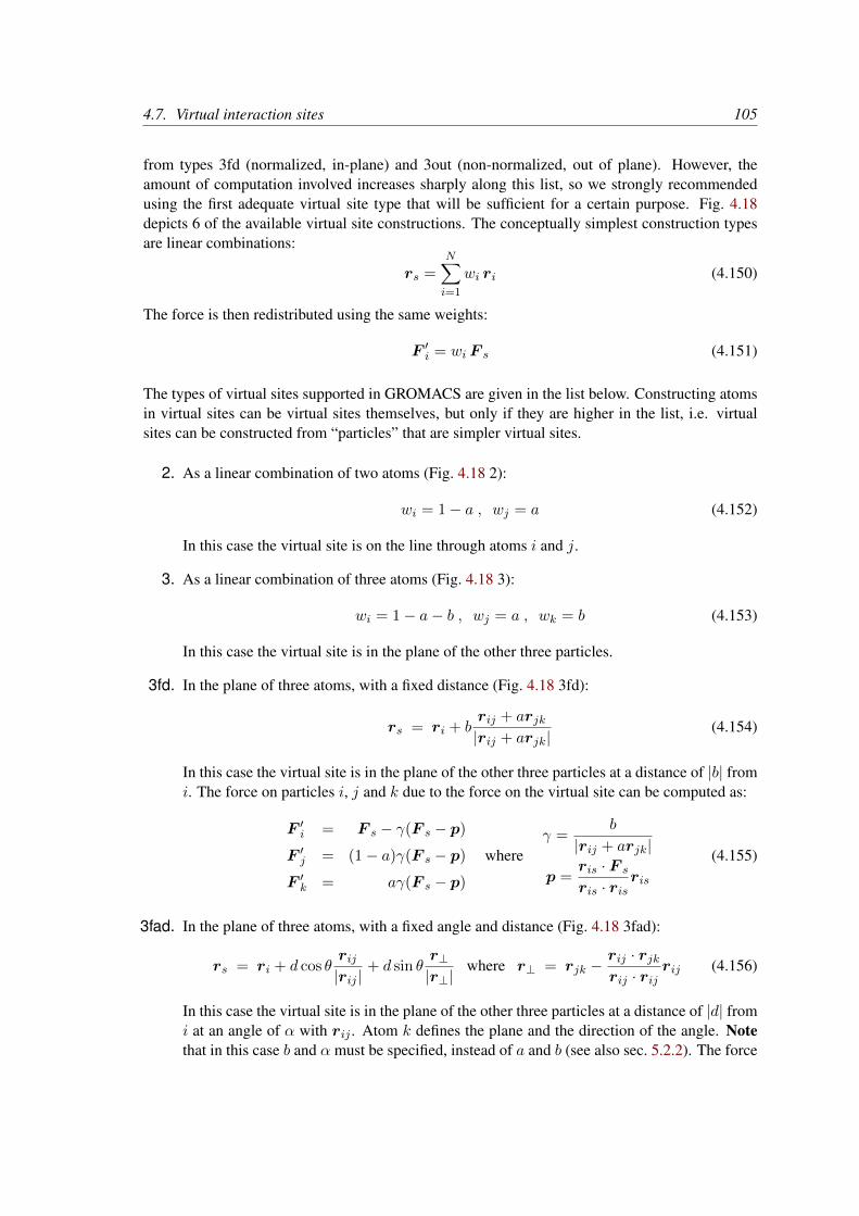
4.7. Virtual interaction sites 105
from types 3fd (normalized, in-plane) and 3out (non-normalized, out of plane). However, theamount of computation involved increases sharply along this list, so we strongly recommendedusing the first adequate virtual site type that will be sufficient for a certain purpose. Fig. 4.18depicts 6 of the available virtual site constructions. The conceptually simplest construction typesare linear combinations:
rs =N∑i=1
wi ri (4.150)
The force is then redistributed using the same weights:
F ′i = wi F s (4.151)
The types of virtual sites supported in GROMACS are given in the list below. Constructing atomsin virtual sites can be virtual sites themselves, but only if they are higher in the list, i.e. virtualsites can be constructed from “particles” that are simpler virtual sites.
2. As a linear combination of two atoms (Fig. 4.18 2):
wi = 1− a , wj = a (4.152)
In this case the virtual site is on the line through atoms i and j.
3. As a linear combination of three atoms (Fig. 4.18 3):
wi = 1− a− b , wj = a , wk = b (4.153)
In this case the virtual site is in the plane of the other three particles.
3fd. In the plane of three atoms, with a fixed distance (Fig. 4.18 3fd):
rs = ri + brij + arjk|rij + arjk|
(4.154)
In this case the virtual site is in the plane of the other three particles at a distance of |b| fromi. The force on particles i, j and k due to the force on the virtual site can be computed as:
F ′i = F s − γ(F s − p)
F ′j = (1− a)γ(F s − p)
F ′k = aγ(F s − p)
whereγ =
b
|rij + arjk|
p =ris · F s
ris · risris
(4.155)
3fad. In the plane of three atoms, with a fixed angle and distance (Fig. 4.18 3fad):
rs = ri + d cos θrij|rij |
+ d sin θr⊥|r⊥|
where r⊥ = rjk −rij · rjkrij · rij
rij (4.156)
In this case the virtual site is in the plane of the other three particles at a distance of |d| fromi at an angle of α with rij . Atom k defines the plane and the direction of the angle. Notethat in this case b and α must be specified, instead of a and b (see also sec. 5.2.2). The force
106 Chapter 4. Interaction function and force fields
on particles i, j and k due to the force on the virtual site can be computed as (with r⊥ asdefined in eqn. 4.156):
F ′i = F s −d cos θ
|rij |F 1 +
d sin θ
|r⊥|
(rij · rjkrij · rij
F 2 + F 3
)
F ′j =d cos θ
|rij |F 1 − d sin θ
|r⊥|
(F 2 +
rij · rjkrij · rij
F 2 + F 3
)
F ′k =d sin θ
|r⊥|F 2
where F 1 = F s −rij · F s
rij · rijrij , F 2 = F 1 −
r⊥ · F s
r⊥ · r⊥r⊥ and F 3 =
rij · F s
rij · rijr⊥
(4.157)
3out. As a non-linear combination of three atoms, out of plane (Fig. 4.18 3out):
rs = ri + arij + brik + c(rij × rik) (4.158)
This enables the construction of virtual sites out of the plane of the other atoms. The forceon particles i, j and k due to the force on the virtual site can be computed as:
F ′j =
a −c zik c yik
c zik a −c xik−c yik c xik a
F s
F ′k =
b c zij −c yij−c zij b c xij
c yij −c xij b
F s
F ′i = F s − F ′j − F ′k
(4.159)
4fdn. From four atoms, with a fixed distance, see separate Fig. 4.19. This construction is a bitcomplex, in particular since the previous type (4fd) could be unstable which forced us tointroduce a more elaborate construction:
rja = a rik − rij = a (xk − xi)− (xj − xi)
rjb = b ril − rij = b (xl − xi)− (xj − xi)
rm = rja × rjb
xs = xi + crm|rm|
(4.160)
In this case the virtual site is at a distance of |c| from i, while a and b are parameters. Notethat the vectors rik and rij are not normalized to save floating-point operations. The forceon particles i, j, k and l due to the force on the virtual site are computed through chain rulederivatives of the construction expression. This is exact and conserves energy, but it does

4.8. Long Range Electrostatics 107
x
xx
x
i
j
k
l
sx
rjajbr
Figure 4.19: The new 4fdn virtual site construction, which is stable even when all constructingatoms are in the same plane.
lead to relatively lengthy expressions that we do not include here (over 200 floating-pointoperations). The interested reader can look at the source code in vsite.c. Fortunately,this vsite type is normally only used for chiral centers such as Cα atoms in proteins.
The new 4fdn construct is identified with a ‘type’ value of 2 in the topology. The earlier4fd type is still supported internally (‘type’ value 1), but it should not be used for newsimulations. All current GROMACS tools will automatically generate type 4fdn instead.
N. A linear combination of N atoms with relative weights ai. The weight for atom i is:
wi = ai
N∑j=1
aj
−1
(4.161)
There are three options for setting the weights:
COG center of geometry: equal weights
COM center of mass: ai is the mass of atom i; when in free-energy simulations the mass ofthe atom is changed, only the mass of the A-state is used for the weight
COW center of weights: ai is defined by the user
4.8 Long Range Electrostatics
4.8.1 Ewald summation
The total electrostatic energy of N particles and their periodic images is given by
V =f
2
∑nx
∑ny
∑nz∗
N∑i
N∑j
qiqjrij,n
. (4.162)

108 Chapter 4. Interaction function and force fields
(nx, ny, nz) = n is the box index vector, and the star indicates that terms with i = j should beomitted when (nx, ny, nz) = (0, 0, 0). The distance rij,n is the real distance between the chargesand not the minimum-image. This sum is conditionally convergent, but very slow.
Ewald summation was first introduced as a method to calculate long-range interactions of the peri-odic images in crystals [110]. The idea is to convert the single slowly-converging sum eqn. 4.162into two quickly-converging terms and a constant term:
V = Vdir + Vrec + V0 (4.163)
Vdir =f
2
N∑i,j
∑nx
∑ny
∑nz∗
qiqjerfc(βrij,n)
rij,n(4.164)
Vrec =f
2πV
N∑i,j
qiqj∑mx
∑my
∑mz∗
exp(−(πm/β)2 + 2πim · (ri − rj)
)m2
(4.165)
V0 = − fβ√π
N∑i
q2i , (4.166)
where β is a parameter that determines the relative weight of the direct and reciprocal sums andm = (mx,my,mz). In this way we can use a short cut-off (of the order of 1 nm) in the directspace sum and a short cut-off in the reciprocal space sum (e.g. 10 wave vectors in each direction).Unfortunately, the computational cost of the reciprocal part of the sum increases as N2 (or N3/2
with a slightly better algorithm) and it is therefore not realistic for use in large systems.
Using Ewald
Don’t use Ewald unless you are absolutely sure this is what you want - for almost all cases the PMEmethod below will perform much better. If you still want to employ classical Ewald summationenter this in your .mdp file, if the side of your box is about 3 nm:
coulombtype = Ewaldrvdw = 0.9rlist = 0.9rcoulomb = 0.9fourierspacing = 0.6ewald-rtol = 1e-5
The ratio of the box dimensions and the fourierspacing parameter determines the highestmagnitude of wave vectors mx,my,mz to use in each direction. With a 3-nm cubic box this ex-ample would use 11 wave vectors (from −5 to 5) in each direction. The ewald-rtol parameteris the relative strength of the electrostatic interaction at the cut-off. Decreasing this gives you amore accurate direct sum, but a less accurate reciprocal sum.
4.8.2 PME
Particle-mesh Ewald is a method proposed by Tom Darden [14] to improve the performance ofthe reciprocal sum. Instead of directly summing wave vectors, the charges are assigned to a grid

4.8. Long Range Electrostatics 109
using interpolation. The implementation in GROMACS uses cardinal B-spline interpolation [15],which is referred to as smooth PME (SPME). The grid is then Fourier transformed with a 3D FFTalgorithm and the reciprocal energy term obtained by a single sum over the grid in k-space.
The potential at the grid points is calculated by inverse transformation, and by using the interpo-lation factors we get the forces on each atom.
The PME algorithm scales as N log(N), and is substantially faster than ordinary Ewald summa-tion on medium to large systems. On very small systems it might still be better to use Ewaldto avoid the overhead in setting up grids and transforms. For the parallelization of PME see thesection on MPMD PME (3.17.5).
With the Verlet cut-off scheme, the PME direct space potential is shifted by a constant such thatthe potential is zero at the cut-off. This shift is small and since the net system charge is close tozero, the total shift is very small, unlike in the case of the Lennard-Jones potential where all shiftsadd up. We apply the shift anyhow, such that the potential is the exact integral of the force.
Using PME
As an example for using Particle-mesh Ewald summation in GROMACS, specify the followinglines in your .mdp file:
coulombtype = PMErvdw = 0.9rlist = 0.9rcoulomb = 0.9fourierspacing = 0.12pme-order = 4ewald-rtol = 1e-5
In this case the fourierspacing parameter determines the maximum spacing for the FFT grid(i.e. minimum number of grid points), and pme-order controls the interpolation order. Usingfourth-order (cubic) interpolation and this spacing should give electrostatic energies accurate toabout 5 · 10−3. Since the Lennard-Jones energies are not this accurate it might even be possible toincrease this spacing slightly.
Pressure scaling works with PME, but be aware of the fact that anisotropic scaling can introduceartificial ordering in some systems.
4.8.3 P3M-AD
The Particle-Particle Particle-Mesh methods of Hockney & Eastwood can also be applied in GRO-MACS for the treatment of long range electrostatic interactions [111]. Although the P3M methodwas the first efficient long-range electrostatics method for molecular simulation, the smooth PME(SPME) method has largely replaced P3M as the method of choice in atomistic simulations. Oneperformance disadvantage of the original P3M method was that it required 3 3D-FFT back trans-forms to obtain the forces on the particles. But this is not required for P3M and the forces can be

110 Chapter 4. Interaction function and force fields
derived through analytical differentiation of the potential, as done in PME. The resulting method istermed P3M-AD. The only remaining difference between P3M-AD and PME is the optimizationof the lattice Green influence function for error minimization that P3M uses. However, in 2012it has been shown that the SPME influence function can be modified to obtain P3M [112]. Thismeans that the advantage of error minimization in P3M-AD can be used at the same computationalcost and with the same code as PME, just by adding a few lines to modify the influence function.However, at optimal parameter setting the effect of error minimization in P3M-AD is less than10%. P3M-AD does show large accuracy gains with interlaced (also known as staggered) grids,but that is not supported in GROMACS (yet).
P3M is used in GROMACS with exactly the same options as used with PME by selecting theelectrostatics type:
coulombtype = P3M-AD
4.8.4 Optimizing Fourier transforms and PME calculations
It is recommended to optimize the parameters for calculation of electrostatic interaction such asPME grid dimensions and cut-off radii. This is particularly relevant to do before launching longproduction runs.
gmx mdrun will automatically do a lot of PME optimization, and GROMACS also includes aspecial tool, gmx tune_pme, which automates the process of selecting the optimal number ofPME-only ranks.
4.9 Long Range Van der Waals interactions
4.9.1 Dispersion correction
In this section, we derive long-range corrections due to the use of a cut-off for Lennard-Jonesor Buckingham interactions. We assume that the cut-off is so long that the repulsion term cansafely be neglected, and therefore only the dispersion term is taken into account. Due to thenature of the dispersion interaction (we are truncating a potential proportional to −r−6), energyand pressure corrections are both negative. While the energy correction is usually small, it may beimportant for free energy calculations where differences between two different Hamiltonians areconsidered. In contrast, the pressure correction is very large and can not be neglected under anycircumstances where a correct pressure is required, especially for any NPT simulations. Althoughit is, in principle, possible to parameterize a force field such that the pressure is close to the desiredexperimental value without correction, such a method makes the parameterization dependent onthe cut-off and is therefore undesirable.
Energy
The long-range contribution of the dispersion interaction to the virial can be derived analytically, ifwe assume a homogeneous system beyond the cut-off distance rc. The dispersion energy between

4.9. Long Range Van der Waals interactions 111
two particles is written as:V (rij) = −C6 r
−6ij (4.167)
and the corresponding force is:F ij = −6C6 r
−8ij rij (4.168)
In a periodic system it is not easy to calculate the full potentials, so usually a cut-off is applied,which can be abrupt or smooth. We will call the potential and force with cut-off Vc and F c. Thelong-range contribution to the dispersion energy in a system with N particles and particle densityρ = N/V is:
Vlr =1
2Nρ
∫ ∞0
4πr2g(r) (V (r)− Vc(r)) dr (4.169)
We will integrate this for the shift function, which is the most general form of van der Waalsinteraction available in GROMACS. The shift function has a constant difference S from 0 to r1
and is 0 beyond the cut-off distance rc. We can integrate eqn. 4.169, assuming that the densityin the sphere within r1 is equal to the global density and the radial distribution function g(r) is 1beyond r1:
Vlr =1
2N
(ρ
∫ r1
04πr2g(r)C6 S dr + ρ
∫ rc
r14πr2 (V (r)− Vc(r)) dr + ρ
∫ ∞rc
4πr2V (r) dr
)=
1
2N
((4
3πρr3
1 − 1
)C6 S + ρ
∫ rc
r14πr2 (V (r)− Vc(r)) dr − 4
3πNρC6 r
−3c
)(4.170)
where the term −1 corrects for the self-interaction. For a plain cut-off we only need to assumethat g(r) is 1 beyond rc and the correction reduces to [113]:
Vlr = −2
3πNρC6 r
−3c (4.171)
If we consider, for example, a box of pure water, simulated with a cut-off of 0.9 nm and a densityof 1 g cm−3 this correction is −0.75 kJ mol−1 per molecule.
For a homogeneous mixture we need to define an average dispersion constant:
〈C6〉 =2
N(N − 1)
N∑i
N∑j>i
C6(i, j) (4.172)
In GROMACS, excluded pairs of atoms do not contribute to the average.
In the case of inhomogeneous simulation systems, e.g. a system with a lipid interface, the energycorrection can be applied if 〈C6〉 for both components is comparable.
Virial and pressure
The scalar virial of the system due to the dispersion interaction between two particles i and j isgiven by:
Ξ = −1
2rij · F ij = 3C6 r
−6ij (4.173)
The pressure is given by:
P =2
3V(Ekin − Ξ) (4.174)

112 Chapter 4. Interaction function and force fields
The long-range correction to the virial is given by:
Ξlr =1
2Nρ
∫ ∞0
4πr2g(r)(Ξ− Ξc) dr (4.175)
We can again integrate the long-range contribution to the virial assuming g(r) is 1 beyond r1:
Ξlr =1
2Nρ
(∫ rc
r14πr2(Ξ− Ξc) dr +
∫ ∞rc
4πr23C6 r−6ij dr
)=
1
2Nρ
(∫ rc
r14πr2(Ξ− Ξc) dr + 4πC6 r
−3c
)(4.176)
For a plain cut-off the correction to the pressure is [113]:
Plr = −4
3πC6 ρ
2r−3c (4.177)
Using the same example of a water box, the correction to the virial is 0.75 kJ mol−1 per molecule,the corresponding correction to the pressure for SPC water is approximately −280 bar.
For homogeneous mixtures, we can again use the average dispersion constant 〈C6〉 (eqn. 4.172):
Plr = −4
3π 〈C6〉 ρ2r−3
c (4.178)
For inhomogeneous systems, eqn. 4.178 can be applied under the same restriction as holds for theenergy (see sec. 4.9.1).
4.9.2 Lennard-Jones PME
In order to treat systems, using Lennard-Jones potentials, that are non-homogeneous outside of thecut-off distance, we can instead use the Particle-mesh Ewald method as discussed for electrostaticsabove. In this case the modified Ewald equations become
V = Vdir + Vrec + V0 (4.179)
Vdir = −1
2
N∑i,j
∑nx
∑ny
∑nz∗
Cij6 g(βrij,n)
rij,n6(4.180)
Vrec =π
32β3
2V
∑mx
∑my
∑mz∗
f(π|m|/β)×N∑i,j
Cij6 exp [−2πim · (ri − rj)] (4.181)
V0 = −β6
12
N∑i
Cii6 (4.182)
where m = (mx,my,mz), β is the parameter determining the weight between direct and recipro-cal space, and Cij6 is the combined dispersion parameter for particle i and j. The star indicates thatterms with i = j should be omitted when ((nx, ny, nz) = (0, 0, 0)), and rij,n is the real distance

4.9. Long Range Van der Waals interactions 113
between the particles. Following the derivation by Essmann [15], the functions f and g introducedabove are defined as
f(x) = 1/3[(1− 2x2)exp(−x2) + 2x3√π erfc(x)
](4.183)
g(x) = exp(−x2)(1 + x2 +x4
2). (4.184)
The above methodology works fine as long as the dispersion parameters can be combined geomet-rically (eqn. 4.6) in the same way as the charges for electrostatics
Cij6,geom =(Cii6 C
jj6
)1/2(4.185)
For Lorentz-Berthelot combination rules (eqn. 4.7), the reciprocal part of this sum has to be cal-culated seven times due to the splitting of the dispersion parameter according to
Cij6,L−B = (σi + σj)6 =
6∑n=0
Pnσni σ
(6−n)j , (4.186)
for Pn the Pascal triangle coefficients. This introduces a non-negligible cost to the reciprocal part,requiring seven separate FFTs, and therefore this has been the limiting factor in previous attemptsto implement LJ-PME. A solution to this problem is to use geometrical combination rules in orderto calculate an approximate interaction parameter for the reciprocal part of the potential, yieldinga total interaction of
V (r < rc) = Cdir6 g(βr)r−6︸ ︷︷ ︸Direct space
+Crecip6,geom[1− g(βr)]r−6︸ ︷︷ ︸
Reciprocal space
= Crecip6,geomr
−6 +(Cdir
6 − Crecip6,geom
)g(βr)r−6 (4.187)
V (r > rc) = Crecip6,geom[1− g(βr)]r−6︸ ︷︷ ︸
Reciprocal space
. (4.188)
This will preserve a well-defined Hamiltonian and significantly increase the performance of thesimulations. The approximation does introduce some errors, but since the difference is located inthe interactions calculated in reciprocal space, the effect will be very small compared to the totalinteraction energy. In a simulation of a lipid bilayer, using a cut-off of 1.0 nm, the relative errorin total dispersion energy was below 0.5%. A more thorough discussion of this can be found in[114].
In GROMACS we now perform the proper calculation of this interaction by subtracting, from thedirect-space interactions, the contribution made by the approximate potential that is used in thereciprocal part
Vdir = Cdir6 r−6 − Crecip
6 [1− g(βr)]r−6. (4.189)
This potential will reduce to the expression in eqn. 4.180 when Cdir6 = Crecip
6 , and the totalinteraction is given by
V (r < rc) = Cdir6 r−6 − Crecip
6 [1− g(βr)]r−6︸ ︷︷ ︸Direct space
+Crecip6 [1− g(βr)]r−6︸ ︷︷ ︸
Reciprocal space
= Cdir6 r−6 (4.190)
V (r > rc) = Crecip6 [1− g(βr)]r−6. (4.191)

114 Chapter 4. Interaction function and force fields
For the case when Cdir6 6= Crecip
6 this will retain an unmodified LJ force up to the cut-off, andthe error is an order of magnitude smaller than in simulations where the direct-space interactionsdo not account for the approximation used in reciprocal space. When using a VdW interactionmodifier of potential-shift, the constant(
−Cdir6 + Crecip
6 [1− g(βrc)])r−6c (4.192)
is added to eqn. 4.190 in order to ensure that the potential is continuous at the cutoff. Notethat, in the same way as eqn. 4.189, this degenerates into the expected −C6g(βrc)r
−6c when
Cdir6 = Crecip
6 . In addition to this, a long-range dispersion correction can be applied to correct forthe approximation using a combination rule in reciprocal space. This correction assumes, as forthe cut-off LJ potential, a uniform particle distribution. But since the error of the combination ruleapproximation is very small this long-range correction is not necessary in most cases. Also notethat this homogenous correction does not correct the surface tension, which is an inhomogeneousproperty.
Using LJ-PME
As an example for using Particle-mesh Ewald summation for Lennard-Jones interactions in GRO-MACS, specify the following lines in your .mdp file:
vdwtype = PMErvdw = 0.9vdw-modifier = Potential-Shiftrlist = 0.9rcoulomb = 0.9fourierspacing = 0.12pme-order = 4ewald-rtol-lj = 0.001lj-pme-comb-rule = geometric
The same Fourier grid and interpolation order are used if both LJ-PME and electrostatic PME areactive, so the settings for fourierspacing and pme-order are common to both. ewald-rtol-ljcontrols the splitting between direct and reciprocal space in the same way as ewald-rtol. In ad-dition to this, the combination rule to be used in reciprocal space is determined by lj-pme-comb-rule.If the current force field uses Lorentz-Berthelot combination rules, it is possible to set lj-pme-comb-rule= geometric in order to gain a significant increase in performance for a small loss in accuracy.The details of this approximation can be found in the section above.
Note that the use of a complete long-range dispersion correction means that as with CoulombPME, rvdw is now a free parameter in the method, rather than being necessarily restricted by theforce-field parameterization scheme. Thus it is now possible to optimize the cutoff, spacing, orderand tolerance terms for accuracy and best performance.
Naturally, the use of LJ-PME rather than LJ cut-off adds computation and communication donefor the reciprocal-space part, so for best performance in balancing the load of parallel simulationsusing PME-only ranks, more such ranks should be used. It may be possible to improve upon theautomatic load-balancing used by mdrun.

4.10. Force field 115
4.10 Force field
A force field is built up from two distinct components:
• The set of equations (called the potential functions) used to generate the potential energiesand their derivatives, the forces. These are described in detail in the previous chapter.
• The parameters used in this set of equations. These are not given in this manual, but in thedata files corresponding to your GROMACS distribution.
Within one set of equations various sets of parameters can be used. Care must be taken that thecombination of equations and parameters form a consistent set. It is in general dangerous to makead hoc changes in a subset of parameters, because the various contributions to the total force areusually interdependent. This means in principle that every change should be documented, verifiedby comparison to experimental data and published in a peer-reviewed journal before it can be used.
GROMACS 2018.5 includes several force fields, and additional ones are available on the website.If you do not know which one to select we recommend GROMOS-96 for united-atom setups andOPLS-AA/L for all-atom parameters. That said, we describe the available options in some detail.
All-hydrogen force field
The GROMOS-87-based all-hydrogen force field is almost identical to the normal GROMOS-87force field, since the extra hydrogens have no Lennard-Jones interaction and zero charge. Theonly differences are in the bond angle and improper dihedral angle terms. This force field is onlyuseful when you need the exact hydrogen positions, for instance for distance restraints derivedfrom NMR measurements. When citing this force field please read the previous paragraph.
4.10.1 GROMOS-96
GROMACS supports the GROMOS-96 force fields [82]. All parameters for the 43A1, 43A2(development, improved alkane dihedrals), 45A3, 53A5, and 53A6 parameter sets are included.All standard building blocks are included and topologies can be built automatically by pdb2gmx.
The GROMOS-96 force field is a further development of the GROMOS-87 force field. It hasimprovements over the GROMOS-87 force field for proteins and small molecules. Note thatthe sugar parameters present in 53A6 do correspond to those published in 2004[115], which aredifferent from those present in 45A4, which is not included in GROMACS at this time. The 45A4parameter set corresponds to a later revision of these parameters. The GROMOS-96 force field isnot, however, recommended for use with long alkanes and lipids. The GROMOS-96 force fielddiffers from the GROMOS-87 force field in a few respects:
• the force field parameters
• the parameters for the bonded interactions are not linked to atom types
• a fourth power bond stretching potential (4.2.1)
116 Chapter 4. Interaction function and force fields
• an angle potential based on the cosine of the angle (4.2.6)
There are two differences in implementation between GROMACS and GROMOS-96 which canlead to slightly different results when simulating the same system with both packages:
• in GROMOS-96 neighbor searching for solvents is performed on the first atom of the solventmolecule. This is not implemented in GROMACS, but the difference with searching bycenters of charge groups is very small
• the virial in GROMOS-96 is molecule-based. This is not implemented in GROMACS,which uses atomic virials
The GROMOS-96 force field was parameterized with a Lennard-Jones cut-off of 1.4 nm, so besure to use a Lennard-Jones cut-off (rvdw) of at least 1.4. A larger cut-off is possible because theLennard-Jones potential and forces are almost zero beyond 1.4 nm.
GROMOS-96 files
GROMACS can read and write GROMOS-96 coordinate and trajectory files. These files shouldhave the extension .g96. Such a file can be a GROMOS-96 initial/final configuration file, acoordinate trajectory file, or a combination of both. The file is fixed format; all floats are writtenas 15.9, and as such, files can get huge. GROMACS supports the following data blocks in thegiven order:
• Header block:
TITLE (mandatory)
• Frame blocks:
TIMESTEP (optional)POSITION/POSITIONRED (mandatory)VELOCITY/VELOCITYRED (optional)BOX (optional)
See the GROMOS-96 manual [82] for a complete description of the blocks. Note that all GRO-MACS programs can read compressed (.Z) or gzipped (.gz) files.
4.10.2 OPLS/AA
4.10.3 AMBER
GROMACS provides native support for the following AMBER force fields:
• AMBER94 [116]

4.10. Force field 117
• AMBER96 [117]
• AMBER99 [118]
• AMBER99SB [119]
• AMBER99SB-ILDN [120]
• AMBER03 [121]
• AMBERGS [122]
4.10.4 CHARMM
GROMACS supports the CHARMM force field for proteins [123, 124], lipids [125] and nucleicacids [126, 127]. The protein parameters (and to some extent the lipid and nucleic acid parameters)were thoroughly tested – both by comparing potential energies between the port and the standardparameter set in the CHARMM molecular simulation package, as well by how the protein forcefield behaves together with GROMACS-specific techniques such as virtual sites (enabling longtime steps) and a fast implicit solvent recently implemented [74] – and the details and results arepresented in the paper by Bjelkmar et al. [128]. The nucleic acid parameters, as well as the onesfor HEME, were converted and tested by Michel Cuendet.
When selecting the CHARMM force field in pdb2gmx the default option is to use CMAP (fortorsional correction map). To exclude CMAP, use -nocmap. The basic form of the CMAP termimplemented in GROMACS is a function of the φ and ψ backbone torsion angles. This term isdefined in the .rtp file by a [ cmap ] statement at the end of each residue supporting CMAP.The following five atom names define the two torsional angles. Atoms 1-4 define φ, and atoms2-5 define ψ. The corresponding atom types are then matched to the correct CMAP type in thecmap.itp file that contains the correction maps.
A port of the CHARMM36 force field for use with GROMACS is also available at http://mackerell.umaryland.edu/charmm_ff.shtml#gromacs.
For branched polymers or other topologies not supported by pdb2gmx, it is possible to use Topo-Tools [129] to generate a GROMACS top file.
4.10.5 Coarse-grained force fields
Coarse-graining is a systematic way of reducing the number of degrees of freedom representinga system of interest. To achieve this, typically whole groups of atoms are represented by singlebeads and the coarse-grained force fields describes their effective interactions. Depending on thechoice of parameterization, the functional form of such an interaction can be complicated andoften tabulated potentials are used.
Coarse-grained models are designed to reproduce certain properties of a reference system. Thiscan be either a full atomistic model or even experimental data. Depending on the properties toreproduce there are different methods to derive such force fields. An incomplete list of methods isgiven below:

118 Chapter 4. Interaction function and force fields
• Conserving free energies
– Simplex method
– MARTINI force field (see next section)
• Conserving distributions (like the radial distribution function), so-called structure-basedcoarse-graining
– (iterative) Boltzmann inversion
– Inverse Monte Carlo
• Conversing forces
– Force matching
Note that coarse-grained potentials are state dependent (e.g. temperature, density,...) and shouldbe re-parametrized depending on the system of interest and the simulation conditions. This canfor example be done using the Versatile Object-oriented Toolkit for Coarse-Graining Applications(VOTCA) [130]. The package was designed to assists in systematic coarse-graining, providesimplementations for most of the algorithms mentioned above and has a well tested interface toGROMACS. It is available as open source and further information can be found at www.votca.org.
4.10.6 MARTINI
The MARTINI force field is a coarse-grain parameter set that allows for the construction of manysystems, including proteins and membranes.
4.10.7 PLUM
The PLUM force field [131] is an example of a solvent-free protein-membrane model for whichthe membrane was derived from structure-based coarse-graining [132]. A GROMACS implemen-tation can be found at code.google.com/p/plumx.

Chapter 5
Topologies
5.1 Introduction
GROMACS must know on which atoms and combinations of atoms the various contributions tothe potential functions (see chapter 4) must act. It must also know what parameters must beapplied to the various functions. All this is described in the topology file *.top, which lists theconstant attributes of each atom. There are many more atom types than elements, but only atomtypes present in biological systems are parameterized in the force field, plus some metals, ions andsilicon. The bonded and special interactions are determined by fixed lists that are included in thetopology file. Certain non-bonded interactions must be excluded (first and second neighbors), asthese are already treated in bonded interactions. In addition, there are dynamic attributes of atoms- their positions, velocities and forces. These do not strictly belong to the molecular topology,and are stored in the coordinate file *.gro (positions and velocities), or trajectory file *.trr(positions, velocities, forces).
This chapter describes the setup of the topology file, the *.top file and the database files: whatthe parameters stand for and how/where to change them if needed. First, all file formats areexplained. Section 5.9.1 describes the organization of the files in each force field.
Note: if you construct your own topologies, we encourage you to upload them to our topologyarchive at www.gromacs.org! Just imagine how thankful you’d have been if your topology hadbeen available there before you started. The same goes for new force fields or modified versionsof the standard force fields - contribute them to the force field archive!
5.2 Particle type
In GROMACS, there are three types of particles, see Table 5.1. Only regular atoms and virtualinteraction sites are used in GROMACS; shells are necessary for polarizable models like the Shell-Water models [45].

120 Chapter 5. Topologies
Particle Symbolatoms Ashells Svirtual interaction sites V (or D)
Table 5.1: Particle types in GROMACS
5.2.1 Atom types
Each force field defines a set of atom types, which have a characteristic name or number, and mass(in a.m.u.). These listings are found in the atomtypes.atp file (.atp = atom type parameterfile). Therefore, it is in this file that you can begin to change and/or add an atom type. A samplefrom the gromos43a1.ff force field is listed below.
O 15.99940 ; carbonyl oxygen (C=O)OM 15.99940 ; carboxyl oxygen (CO-)OA 15.99940 ; hydroxyl, sugar or ester oxygenOW 15.99940 ; water oxygenN 14.00670 ; peptide nitrogen (N or NH)NT 14.00670 ; terminal nitrogen (NH2)NL 14.00670 ; terminal nitrogen (NH3)NR 14.00670 ; aromatic nitrogenNZ 14.00670 ; Arg NH (NH2)NE 14.00670 ; Arg NE (NH)C 12.01100 ; bare carbon
CH1 13.01900 ; aliphatic or sugar CH-groupCH2 14.02700 ; aliphatic or sugar CH2-groupCH3 15.03500 ; aliphatic CH3-group
Note: GROMACS makes use of the atom types as a name, not as a number (as e.g. in GROMOS).
5.2.2 Virtual sites
Some force fields use virtual interaction sites (interaction sites that are constructed from otherparticle positions) on which certain interactions are located (e.g. on benzene rings, to reproducethe correct quadrupole). This is described in sec. 4.7.
To make virtual sites in your system, you should include a section [ virtual_sites? ] (forbackward compatibility the old name [ dummies? ] can also be used) in your topology file,where the ‘?’ stands for the number constructing particles for the virtual site. This will be ‘2’ fortype 2, ‘3’ for types 3, 3fd, 3fad and 3out and ‘4’ for type 4fdn. The last of these replace an older4fd type (with the ‘type’ value 1) that could occasionally be unstable; while it is still supportedinternally in the code, the old 4fd type should not be used in new input files. The different typesare explained in sec. 4.7.
Parameters for type 2 should look like this:
[ virtual_sites2 ]

5.2. Particle type 121
; Site from funct a5 1 2 1 0.7439756
for type 3 like this:
[ virtual_sites3 ]; Site from funct a b5 1 2 3 1 0.7439756 0.128012
for type 3fd like this:
[ virtual_sites3 ]; Site from funct a d5 1 2 3 2 0.5 -0.105
for type 3fad like this:
[ virtual_sites3 ]; Site from funct theta d5 1 2 3 3 120 0.5
for type 3out like this:
[ virtual_sites3 ]; Site from funct a b c5 1 2 3 4 -0.4 -0.4 6.9281
for type 4fdn like this:
[ virtual_sites4 ]; Site from funct a b c5 1 2 3 4 2 1.0 0.9 0.105
This will result in the construction of a virtual site, number 5 (first column ‘Site’), based on thepositions of the atoms whose indices are 1 and 2 or 1, 2 and 3 or 1, 2, 3 and 4 (next two, threeor four columns ‘from’) following the rules determined by the function number (next column‘funct’) with the parameters specified (last one, two or three columns ‘a b . .’). Obviously,the atom numbers (including virtual site number) depend on the molecule. It may be instructiveto study the topologies for TIP4P or TIP5P water models that are included with the GROMACSdistribution.
Note that if any constant bonded interactions are defined between virtual sites and/or normalatoms, they will be removed by grompp (unless the option tt -normvsbds is used). This re-moval of bonded interactions is done after generating exclusions, as the generation of exclusionsis based on “chemically” bonded interactions.
Virtual sites can be constructed in a more generic way using basic geometric parameters. The di-rective that can be used is [ virtual_sitesn ]. Required parameters are listed in Table 5.5.An example entry for defining a virtual site at the center of geometry of a given set of atoms mightbe:
[ virtual_sitesn ]; Site funct from5 1 1 2 3 4

122 Chapter 5. Topologies
Property Symbol UnitType - -Mass m a.m.u.Charge q electronepsilon ε kJ/molsigma σ nm
Table 5.2: Static atom type properties in GROMACS
5.3 Parameter files
5.3.1 Atoms
The static properties (see Table 5.2 assigned to the atom types are assigned based on data in severalplaces. The mass is listed in atomtypes.atp (see 5.2.1), whereas the charge is listed in *.rtp(.rtp = residue topology parameter file, see 5.7.1). This implies that the charges are only definedin the building blocks of amino acids, nucleic acids or otherwise, as defined by the user. Whengenerating a topology (*.top) using the pdb2gmx program, the information from these files iscombined.
5.3.2 Non-bonded parameters
The non-bonded parameters consist of the van der Waals parameters V (c6 or σ, depending on thecombination rule) and W (c12 or ε), as listed in the file ffnonbonded.itp, where ptype isthe particle type (see Table 5.1). As with the bonded parameters, entries in [ *type ] directivesare applied to their counterparts in the topology file. Missing parameters generate warnings, exceptas noted below in section 5.4.3.
[ atomtypes ];name at.num mass charge ptype V(c6) W(c12)
O 8 15.99940 0.000 A 0.22617E-02 0.74158E-06OM 8 15.99940 0.000 A 0.22617E-02 0.74158E-06.....
[ nonbond_params ]; i j func V(c6) W(c12)
O O 1 0.22617E-02 0.74158E-06O OA 1 0.22617E-02 0.13807E-05.....
Note that most of the included force fields also include the at.num. column, but this same in-formation is implied in the OPLS-AA bond_type column. The interpretation of the parametersV and W depends on the combination rule that was chosen in the [ defaults ] section of thetopology file (see 5.8.1):
for combination rule 1 :Vii = C
(6)i = 4 εiσ
6i [ kJ mol−1 nm6 ]
Wii = C(12)i = 4 εiσ
12i [ kJ mol−1 nm12 ]
(5.1)

5.3. Parameter files 123
for combination rules 2 and 3 :Vii = σi [ nm ]Wii = εi [ kJ mol−1 ]
(5.2)
Some or all combinations for different atom types can be given in the [ nonbond_params ]section, again with parameters V and W as defined above. Any combination that is not given willbe computed from the parameters for the corresponding atom types, according to the combinationrule:
for combination rules 1 and 3 :C
(6)ij =
(C
(6)i C
(6)j
) 12
C(12)ij =
(C
(12)i C
(12)j
) 12
(5.3)
for combination rule 2 :σij = 1
2(σi + σj)εij =
√εi εj
(5.4)
When σ and ε need to be supplied (rules 2 and 3), it would seem it is impossible to have a non-zeroC12 combined with a zero C6 parameter. However, providing a negative σ will do exactly that,such that C6 is set to zero and C12 is calculated normally. This situation represents a special casein reading the value of σ, and nothing more.
There is only one set of combination rules for Buckingham potentials:
Aij = (AiiAjj)1/2
Bij = 2/(
1Bii
+ 1Bjj
)Cij = (CiiCjj)
1/2
(5.5)
5.3.3 Bonded parameters
The bonded parameters (i.e. bonds, bond angles, improper and proper dihedrals) are listed inffbonded.itp. The entries in this database describe, respectively, the atom types in the in-teractions, the type of the interaction, and the parameters associated with that interaction. Theseparameters are then read by grompp when processing a topology and applied to the relevantbonded parameters, i.e. bondtypes are applied to entries in the [ bonds ] directive, etc.Any bonded parameter that is missing from the relevant [ *type ] directive generates a fatalerror. The types of interactions are listed in Table 5.5. Example excerpts from such files follow:
[ bondtypes ]; i j func b0 kb
C O 1 0.12300 502080.C OM 1 0.12500 418400.......
[ angletypes ]; i j k func th0 cthHO OA C 1 109.500 397.480HO OA CH1 1 109.500 397.480......
[ dihedraltypes ]

124 Chapter 5. Topologies
; i l func q0 cqNR5* NR5 2 0.000 167.360NR5* NR5* 2 0.000 167.360......
[ dihedraltypes ]; j k func phi0 cp mult
C OA 1 180.000 16.736 2C N 1 180.000 33.472 2......
[ dihedraltypes ];; Ryckaert-Bellemans Dihedrals;; aj ak functCP2 CP2 3 9.2789 12.156 -13.120 -3.0597 26.240 -31.495
In the ffbonded.itp file, you can add bonded parameters. If you want to include parametersfor new atom types, make sure you define them in atomtypes.atp as well.
For most interaction types, bonded parameters are searched and assigned using an exact match forall type names and allowing only a single set of parameters. The exception to this rule are dihedralparameters. For [ dihedraltypes ] wildcard atom type names can be specified with theletter X in one or more of the four positions. Thus one can for example assign proper dihedralparameters based on the types of the middle two atoms. The parameters for the entry with themost exact matches, i.e. the least wildcard matches, will be used. Note that GROMACS versionsolder than 5.1.3 used the first match, which means that a full match would be ignored if it ispreceded by an entry that matches on wildcards. Thus it is suggested to put wildcard entries at theend, in case someone might use a forcefield with older versions of GROMACS. In addition thereis a dihedral type 9 which adds the possibility of assigning multiple dihedral potentials, usefulfor combining terms with different multiplicities. The different dihedral potential parameter setsshould be on directly adjacent lines in the [ dihedraltypes ] section.
5.4 Molecule definition
5.4.1 Moleculetype entries
An organizational structure that usually corresponds to molecules is the [ moleculetype ]entry. This entry serves two main purposes. One is to give structure to the topology file(s), usu-ally corresponding to real molecules. This makes the topology easier to read and writing it lesslabor intensive. A second purpose is computational efficiency. The system definition that is keptin memory is proportional in size of the moleculetype definitions. If a molecule is presentin 100000 copies, this saves a factor of 100000 in memory, which means the system usually fitsin cache, which can improve performance tremendously. Interactions that correspond to chemicalbonds, that generate exclusions, can only be defined between atoms within a moleculetype. Itis allowed to have multiple molecules which are not covalently bonded in one moleculetype

5.4. Molecule definition 125
definition. Molecules can be made infinitely long by connecting to themselves over periodicboundaries. When such periodic molecules are present, an option in the mdp file needs to beset to tell GROMACS not to attempt to make molecules that are broken over periodic boundarieswhole again.
5.4.2 Intermolecular interactions
In some cases, one would like atoms in different molecules to also interact with other interac-tions than the usual non-bonded interactions. This is often the case in binding studies. Whenthe molecules are covalently bound, e.g. a ligand binding covalently to a protein, they are effec-tively one molecule and they should be defined in one [ moleculetype ] entry. Note thatpdb2gmx has an option to put two or more molecules in one [ moleculetype ] entry. Whenmolecules are not covalently bound, it is much more convenient to use separate moleculetypedefinitions and specify the intermolecular interactions in the [ intermolecular_interactions]section. In this section, which is placed at the end of the topology (see Table 5.4), normal bondedinteractions can be specified using global atom indices. The only restrictions are that no interac-tions can be used that generates exclusions and no constraints can be used.
5.4.3 Intramolecular pair interactions
Extra Lennard-Jones and electrostatic interactions between pairs of atoms in a molecule can beadded in the [ pairs ] section of a molecule definition. The parameters for these interactionscan be set independently from the non-bonded interaction parameters. In the GROMOS forcefields, pairs are only used to modify the 1-4 interactions (interactions of atoms separated by threebonds). In these force fields the 1-4 interactions are excluded from the non-bonded interactions(see sec. 5.4.4).
[ pairtypes ]; i j func cs6 cs12 ; THESE ARE 1-4 INTERACTIONS
O O 1 0.22617E-02 0.74158E-06O OM 1 0.22617E-02 0.74158E-06.....
The pair interaction parameters for the atom types in ffnonbonded.itp are listed in the[ pairtypes ] section. The GROMOS force fields list all these interaction parameters explic-itly, but this section might be empty for force fields like OPLS that calculate the 1-4 interactions byuniformly scaling the parameters. Pair parameters that are not present in the [ pairtypes ]section are only generated when gen-pairs is set to “yes” in the [ defaults ] directive offorcefield.itp (see 5.8.1). When gen-pairs is set to “no,” grompp will give a warningfor each pair type for which no parameters are given.
The normal pair interactions, intended for 1-4 interactions, have function type 1. Function type 2and the [ pairs_nb ] are intended for free-energy simulations. When determining hydrationfree energies, the solute needs to be decoupled from the solvent. This can be done by adding aB-state topology (see sec. 3.12) that uses zero for all solute non-bonded parameters, i.e. charges

126 Chapter 5. Topologies
and LJ parameters. However, the free energy difference between the A and B states is not the totalhydration free energy. One has to add the free energy for reintroducing the internal Coulomb andLJ interactions in the solute when in vacuum. This second step can be combined with the first stepwhen the Coulomb and LJ interactions within the solute are not modified. For this purpose, there isa pairs function type 2, which is identical to function type 1, except that the B-state parameters arealways identical to the A-state parameters. For searching the parameters in the [ pairtypes ]section, no distinction is made between function type 1 and 2. The pairs section [ pairs_nb ]is intended to replace the non-bonded interaction. It uses the unscaled charges and the non-bondedLJ parameters; it also only uses the A-state parameters. Note that one should add exclusions forall atom pairs listed in [ pairs_nb ], otherwise such pairs will also end up in the normalneighbor lists.
Alternatively, this same behavior can be achieved without ever touching the topology, by usingthe couple-moltype, couple-lambda0, couple-lambda1, and couple-intramolkeywords. See sections sec. 3.12 and sec. 6.1 for more information.
All three pair types always use plain Coulomb interactions, even when Reaction-field, PME, Ewaldor shifted Coulomb interactions are selected for the non-bonded interactions. Energies for types1 and 2 are written to the energy and log file in separate “LJ-14” and “Coulomb-14” entries perenergy group pair. Energies for [ pairs_nb ] are added to the “LJ-(SR)” and “Coulomb-(SR)” terms.
5.4.4 Exclusions
The exclusions for non-bonded interactions are generated by grompp for neighboring atoms upto a certain number of bonds away, as defined in the [ moleculetype ] section in the topol-ogy file (see 5.8.1). Particles are considered bonded when they are connected by “chemical”bonds ([ bonds ] types 1 to 5, 7 or 8) or constraints ([ constraints ] type 1). Type 5[ bonds ] can be used to create a connection between two atoms without creating an interac-tion. There is a harmonic interaction ([ bonds ] type 6) that does not connect the atoms by achemical bond. There is also a second constraint type ([ constraints ] type 2) that fixesthe distance, but does not connect the atoms by a chemical bond. For a complete list of all theseinteractions, see Table 5.5.
Extra exclusions within a molecule can be added manually in a [ exclusions ] section. Eachline should start with one atom index, followed by one or more atom indices. All non-bondedinteractions between the first atom and the other atoms will be excluded.
When all non-bonded interactions within or between groups of atoms need to be excluded, is itmore convenient and much more efficient to use energy monitor group exclusions (see sec. 3.3).
5.5 Implicit solvation parameters
Starting with GROMACS 4.5, implicit solvent is supported. A section in the topology has beenintroduced to list those parameters:
[ implicit_genborn_params ]
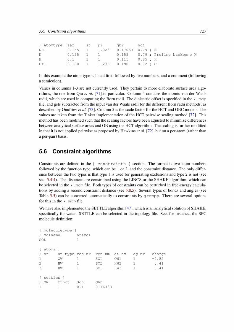
5.6. Constraint algorithms 127
; Atomtype sar st pi gbr hctNH1 0.155 1 1.028 0.17063 0.79 ; NN 0.155 1 1 0.155 0.79 ; Proline backbone NH 0.1 1 1 0.115 0.85 ; HCT1 0.180 1 1.276 0.190 0.72 ; C
In this example the atom type is listed first, followed by five numbers, and a comment (followinga semicolon).
Values in columns 1-3 are not currently used. They pertain to more elaborate surface area algo-rithms, the one from Qiu et al. [71] in particular. Column 4 contains the atomic van der Waalsradii, which are used in computing the Born radii. The dielectric offset is specified in the *.mdpfile, and gets subtracted from the input van der Waals radii for the different Born radii methods, asdescribed by Onufriev et al. [73]. Column 5 is the scale factor for the HCT and OBC models. Thevalues are taken from the Tinker implementation of the HCT pairwise scaling method [72]. Thismethod has been modified such that the scaling factors have been adjusted to minimize differencesbetween analytical surface areas and GB using the HCT algorithm. The scaling is further modifiedin that it is not applied pairwise as proposed by Hawkins et al. [72], but on a per-atom (rather thana per-pair) basis.
5.6 Constraint algorithms
Constraints are defined in the [ constraints ] section. The format is two atom numbersfollowed by the function type, which can be 1 or 2, and the constraint distance. The only differ-ence between the two types is that type 1 is used for generating exclusions and type 2 is not (seesec. 5.4.4). The distances are constrained using the LINCS or the SHAKE algorithm, which canbe selected in the *.mdp file. Both types of constraints can be perturbed in free-energy calcula-tions by adding a second constraint distance (see 5.8.5). Several types of bonds and angles (seeTable 5.5) can be converted automatically to constraints by grompp. There are several optionsfor this in the *.mdp file.
We have also implemented the SETTLE algorithm [47], which is an analytical solution of SHAKE,specifically for water. SETTLE can be selected in the topology file. See, for instance, the SPCmolecule definition:
[ moleculetype ]; molname nrexclSOL 1
[ atoms ]; nr at type res nr ren nm at nm cg nr charge1 OW 1 SOL OW1 1 -0.822 HW 1 SOL HW2 1 0.413 HW 1 SOL HW3 1 0.41
[ settles ]; OW funct doh dhh1 1 0.1 0.16333
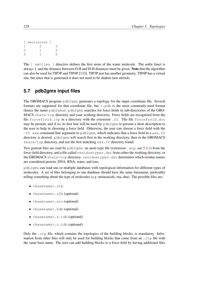
128 Chapter 5. Topologies
[ exclusions ]1 2 32 1 33 1 2
The [ settles ] directive defines the first atom of the water molecule. The settle funct isalways 1, and the distance between O-H and H-H distances must be given. Note that the algorithmcan also be used for TIP3P and TIP4P [133]. TIP3P just has another geometry. TIP4P has a virtualsite, but since that is generated it does not need to be shaken (nor stirred).
5.7 pdb2gmx input files
The GROMACS program pdb2gmx generates a topology for the input coordinate file. Severalformats are supported for that coordinate file, but *.pdb is the most commonly-used format(hence the name pdb2gmx). pdb2gmx searches for force fields in sub-directories of the GRO-MACS share/top directory and your working directory. Force fields are recognized from thefile forcefield.itp in a directory with the extension .ff. The file forcefield.docmay be present, and if so, its first line will be used by pdb2gmx to present a short description tothe user to help in choosing a force field. Otherwise, the user can choose a force field with the-ff xxx command-line argument to pdb2gmx, which indicates that a force field in a xxx.ffdirectory is desired. pdb2gmx will search first in the working directory, then in the GROMACSshare/top directory, and use the first matching xxx.ff directory found.
Two general files are read by pdb2gmx: an atom type file (extension .atp, see 5.2.1) from theforce-field directory, and a file called residuetypes.dat from either the working directory, orthe GROMACS share/top directory. residuetypes.dat determines which residue namesare considered protein, DNA, RNA, water, and ions.
pdb2gmx can read one or multiple databases with topological information for different types ofmolecules. A set of files belonging to one database should have the same basename, preferablytelling something about the type of molecules (e.g. aminoacids, rna, dna). The possible files are:
• <basename>.rtp
• <basename>.r2b (optional)
• <basename>.arn (optional)
• <basename>.hdb (optional)
• <basename>.n.tdb (optional)
• <basename>.c.tdb (optional)
Only the .rtp file, which contains the topologies of the building blocks, is mandatory. Infor-mation from other files will only be used for building blocks that come from an .rtp file withthe same base name. The user can add building blocks to a force field by having additional files

5.7. pdb2gmx input files 129
with the same base name in their working directory. By default, only extra building blocks can bedefined, but calling pdb2gmx with the -rtpo option will allow building blocks in a local file toreplace the default ones in the force field.
5.7.1 Residue database
The files holding the residue databases have the extension .rtp. Originally this file containedbuilding blocks (amino acids) for proteins, and is the GROMACS interpretation of the rt37c4.datfile of GROMOS. So the residue database file contains information (bonds, charges, charge groups,and improper dihedrals) for a frequently-used building block. It is better not to change this filebecause it is standard input for pdb2gmx, but if changes are needed make them in the *.top file(see 5.8.1), or in a .rtp file in the working directory as explained in sec. 5.7. Defining topologiesof new small molecules is probably easier by writing an include topology file *.itp directly.This will be discussed in section 5.8.2. When adding a new protein residue to the database, don’tforget to add the residue name to the residuetypes.dat file, so that grompp, make_ndxand analysis tools can recognize the residue as a protein residue (see 8.1.1).
The .rtp files are only used by pdb2gmx. As mentioned before, the only extra information thisprogram needs from the .rtp database is bonds, charges of atoms, charge groups, and improperdihedrals, because the rest is read from the coordinate input file. Some proteins contain residuesthat are not standard, but are listed in the coordinate file. You have to construct a building block forthis “strange” residue, otherwise you will not obtain a *.top file. This also holds for moleculesin the coordinate file such as ligands, polyatomic ions, crystallization co-solvents, etc. The residuedatabase is constructed in the following way:
[ bondedtypes ] ; mandatory; bonds angles dihedrals impropers
1 1 1 2 ; mandatory
[ GLY ] ; mandatory
[ atoms ] ; mandatory; name type charge chargegroup
N N -0.280 0H H 0.280 0
CA CH2 0.000 1C C 0.380 2O O -0.380 2
[ bonds ] ; optional;atom1 atom2 b0 kb
N HN CA
CA CC O
-C N
[ exclusions ] ; optional;atom1 atom2

130 Chapter 5. Topologies
[ angles ] ; optional;atom1 atom2 atom3 th0 cth
[ dihedrals ] ; optional;atom1 atom2 atom3 atom4 phi0 cp mult
[ impropers ] ; optional;atom1 atom2 atom3 atom4 q0 cq
N -C CA H-C -CA N -O
[ ZN ]
[ atoms ]ZN ZN 2.000 0
The file is free format; the only restriction is that there can be at most one entry on a line. The firstfield in the file is the [ bondedtypes ] field, which is followed by four numbers, indicatingthe interaction type for bonds, angles, dihedrals, and improper dihedrals. The file contains residueentries, which consist of atoms and (optionally) bonds, angles, dihedrals, and impropers. Thecharge group codes denote the charge group numbers. Atoms in the same charge group shouldalways be ordered consecutively. When using the hydrogen database with pdb2gmx for addingmissing hydrogens (see 5.7.4), the atom names defined in the .rtp entry should correspond ex-actly to the naming convention used in the hydrogen database. The atom names in the bondedinteraction can be preceded by a minus or a plus, indicating that the atom is in the preceding orfollowing residue respectively. Explicit parameters added to bonds, angles, dihedrals, and im-propers override the standard parameters in the .itp files. This should only be used in specialcases. Instead of parameters, a string can be added for each bonded interaction. This is used inGROMOS-96 .rtp files. These strings are copied to the topology file and can be replaced byforce-field parameters by the C-preprocessor in grompp using #define statements.
pdb2gmx automatically generates all angles. This means that for most force fields the [ angles ]field is only useful for overriding .itp parameters. For the GROMOS-96 force field the interac-tion number of all angles needs to be specified.
pdb2gmx automatically generates one proper dihedral for every rotatable bond, preferably onheavy atoms. When the [ dihedrals ] field is used, no other dihedrals will be generated forthe bonds corresponding to the specified dihedrals. It is possible to put more than one dihedralfunction on a rotatable bond. In the case of CHARMM27 FF pdb2gmx can add correction mapsto the dihedrals using the default -cmap option. Please refer to 4.10.4 for more information.
pdb2gmx sets the number of exclusions to 3, which means that interactions between atoms con-nected by at most 3 bonds are excluded. Pair interactions are generated for all pairs of atomsthat are separated by 3 bonds (except pairs of hydrogens). When more interactions need to beexcluded, or some pair interactions should not be generated, an [ exclusions ] field can beadded, followed by pairs of atom names on separate lines. All non-bonded and pair interactionsbetween these atoms will be excluded.

5.7. pdb2gmx input files 131
ARG protonated arginineARGN neutral arginineASP negatively charged aspartic acidASPH neutral aspartic acidCYS neutral cysteineCYS2 cysteine with sulfur bound to another cysteine or a hemeGLU negatively charged glutamic acidGLUH neutral glutamic acidHISD neutral histidine with Nδ protonatedHISE neutral histidine with Nε protonatedHISH positive histidine with both Nδ and Nε protonatedHIS1 histidine bound to a hemeLYSN neutral lysineLYS protonated lysineHEME heme
Table 5.3: Internal GROMACS residue naming convention.
5.7.2 Residue to building block database
Each force field has its own naming convention for residues. Most residues have consistent nam-ing, but some, especially those with different protonation states, can have many different names.The .r2b files are used to convert standard residue names to the force-field build block names. Ifno .r2b is present in the force-field directory or a residue is not listed, the building block name isassumed to be identical to the residue name. The .r2b can contain 2 or 5 columns. The 2-columnformat has the residue name in the first column and the building block name in the second. The5-column format has 3 additional columns with the building block for the residue occurring inthe N-terminus, C-terminus and both termini at the same time (single residue molecule). This isuseful for, for instance, the AMBER force fields. If one or more of the terminal versions are notpresent, a dash should be entered in the corresponding column.
There is a GROMACS naming convention for residues which is only apparent (except for thepdb2gmx code) through the .r2b file and specbond.dat files. This convention is only ofimportance when you are adding residue types to an .rtp file. The convention is listed in Ta-ble 5.3. For special bonds with, for instance, a heme group, the GROMACS naming conventionis introduced through specbond.dat (see 5.7.7), which can subsequently be translated by the.r2b file, if required.
5.7.3 Atom renaming database
Force fields often use atom names that do not follow IUPAC or PDB convention. The .arndatabase is used to translate the atom names in the coordinate file to the force-field names. Atomsthat are not listed keep their names. The file has three columns: the building block name, theold atom name, and the new atom name, respectively. The residue name supports question-markwildcards that match a single character.

132 Chapter 5. Topologies
An additional general atom renaming file called xlateat.dat is present in the share/topdirectory, which translates common non-standard atom names in the coordinate file to IUPAC/PDBconvention. Thus, when writing force-field files, you can assume standard atom names and nofurther atom name translation is required, except for translating from standard atom names to theforce-field ones.
5.7.4 Hydrogen database
The hydrogen database is stored in .hdb files. It contains information for the pdb2gmx programon how to connect hydrogen atoms to existing atoms. In versions of the database before GRO-MACS 3.3, hydrogen atoms were named after the atom they are connected to: the first letter ofthe atom name was replaced by an ‘H.’ In the versions from 3.3 onwards, the H atom has to belisted explicitly, because the old behavior was protein-specific and hence could not be generalizedto other molecules. If more than one hydrogen atom is connected to the same atom, a number willbe added to the end of the hydrogen atom name. For example, adding two hydrogen atoms to ND2(in asparagine), the hydrogen atoms will be named HD21 and HD22. This is important since atomnaming in the .rtp file (see 5.7.1) must be the same. The format of the hydrogen database is asfollows:
; res # additions# H add type H i j k
ALA 11 1 H N -C CA
ARG 41 2 H N CA C1 1 HE NE CD CZ2 3 HH1 NH1 CZ NE2 3 HH2 NH2 CZ NE
On the first line we see the residue name (ALA or ARG) and the number of kinds of hydrogenatoms that may be added to this residue by the hydrogen database. After that follows one line foreach addition, on which we see:
• The number of H atoms added
• The method for adding H atoms, which can be any of:
1 one planar hydrogen, e.g. rings or peptide bondOne hydrogen atom (n) is generated, lying in the plane of atoms (i,j,k) on the planebisecting angle (j-i-k) at a distance of 0.1 nm from atom i, such that the angles (n-i-j)and (n-i-k) are > 90o.
2 one single hydrogen, e.g. hydroxylOne hydrogen atom (n) is generated at a distance of 0.1 nm from atom i, such thatangle (n-i-j)=109.5 degrees and dihedral (n-i-j-k)=trans.
3 two planar hydrogens, e.g. ethylene -C=CH2, or amide -C(=O)NH2
Two hydrogens (n1,n2) are generated at a distance of 0.1 nm from atom i, such that

5.7. pdb2gmx input files 133
angle (n1-i-j)=(n2-i-j)=120 degrees and dihedral (n1-i-j-k)=cis and (n2-i-j-k)=trans,such that names are according to IUPAC standards [134].
4 two or three tetrahedral hydrogens, e.g. -CH3
Three (n1,n2,n3) or two (n1,n2) hydrogens are generated at a distance of 0.1 nm fromatom i, such that angle (n1-i-j)=(n2-i-j)=(n3-i-j)=109.47o, dihedral (n1-i-j-k)=trans,(n2-i-j-k)=trans+120 and (n3-i-j-k)=trans+240o.
5 one tetrahedral hydrogen, e.g. C3CHOne hydrogen atom (n′) is generated at a distance of 0.1 nm from atom i in tetrahedralconformation such that angle (n′-i-j)=(n′-i-k)=(n′-i-l)=109.47o.
6 two tetrahedral hydrogens, e.g. C-CH2-CTwo hydrogen atoms (n1,n2) are generated at a distance of 0.1 nm from atom i intetrahedral conformation on the plane bisecting angle j-i-k with angle (n1-i-n2)=(n1-i-j)=(n1-i-k)=109.47o.
7 two water hydrogensTwo hydrogens are generated around atom i according to SPC [85] water geometry.The symmetry axis will alternate between three coordinate axes in both directions.
10 three water “hydrogens”Two hydrogens are generated around atom i according to SPC [85] water geometry.The symmetry axis will alternate between three coordinate axes in both directions.In addition, an extra particle is generated on the position of the oxygen with the firstletter of the name replaced by ‘M’. This is for use with four-atom water models suchas TIP4P [133].
11 four water “hydrogens”Same as above, except that two additional particles are generated on the position ofthe oxygen, with names ‘LP1’ and ‘LP2.’ This is for use with five-atom water modelssuch as TIP5P [135].
• The name of the new H atom (or its prefix, e.g. HD2 for the asparagine example givenearlier).
• Three or four control atoms (i,j,k,l), where the first always is the atom to which the H atomsare connected. The other two or three depend on the code selected. For water, there is onlyone control atom.
Some more exotic cases can be approximately constructed from the above tools, and with suit-able use of energy minimization are good enough for beginning MD simulations. For examplesecondary amine hydrogen, nitrenyl hydrogen (C=NH) and even ethynyl hydrogen could be ap-proximately constructed using method 2 above for hydroxyl hydrogen.
5.7.5 Termini database
The termini databases are stored in aminoacids.n.tdb and aminoacids.c.tdb for the N-and C-termini respectively. They contain information for the pdb2gmx program on how to con-nect new atoms to existing ones, which atoms should be removed or changed, and which bondedinteractions should be added. Their format is as follows (from gromos43a1.ff/aminoacids.c.tdb):

134 Chapter 5. Topologies
[ None ]
[ COO- ][ replace ]C C C 12.011 0.27O O1 OM 15.9994 -0.635OXT O2 OM 15.9994 -0.635[ add ]2 8 O C CA NOM 15.9994 -0.635[ bonds ]C O1 gb_5C O2 gb_5[ angles ]O1 C O2 ga_37CA C O1 ga_21CA C O2 ga_21[ dihedrals ]N CA C O2 gd_20[ impropers ]C CA O2 O1 gi_1
The file is organized in blocks, each with a header specifying the name of the block. Theseblocks correspond to different types of termini that can be added to a molecule. In this example[ COO- ] is the first block, corresponding to changing the terminal carbon atom into a depro-tonated carboxyl group. [ None ] is the second terminus type, corresponding to a terminusthat leaves the molecule as it is. Block names cannot be any of the following: replace, add,delete, bonds, angles, dihedrals, impropers. Doing so would interfere with the pa-rameters of the block, and would probably also be very confusing to human readers.
For each block the following options are present:
• [ replace ]Replace an existing atom by one with a different atom type, atom name, charge, and/ormass. This entry can be used to replace an atom that is present both in the input coordinatesand in the .rtp database, but also to only rename an atom in the input coordinates suchthat it matches the name in the force field. In the latter case, there should also be a corre-sponding [ add ] section present that gives instructions to add the same atom, such thatthe position in the sequence and the bonding is known. Such an atom can be present in theinput coordinates and kept, or not present and constructed by pdb2gmx. For each atom tobe replaced on line should be entered with the following fields:
– name of the atom to be replaced
– new atom name (optional)
– new atom type
– new mass
– new charge

5.7. pdb2gmx input files 135
• [ add ]Add new atoms. For each (group of) added atom(s), a two-line entry is necessary. Thefirst line contains the same fields as an entry in the hydrogen database (name of the newatom, number of atoms, type of addition, control atoms, see 5.7.4), but the possible types ofaddition are extended by two more, specifically for C-terminal additions:
8 two carboxyl oxygens, -COO−
Two oxygens (n1,n2) are generated according to rule 3, at a distance of 0.136 nm fromatom i and an angle (n1-i-j)=(n2-i-j)=117 degrees
9 carboxyl oxygens and hydrogen, -COOHTwo oxygens (n1,n2) are generated according to rule 3, at distances of 0.123 nm and0.125 nm from atom i for n1 and n2, respectively, and angles (n1-i-j)=121 and (n2-i-j)=115 degrees. One hydrogen (n′) is generated around n2 according to rule 2, wheren-i-j and n-i-j-k should be read as n′-n2-i and n′-n2-i-j, respectively.
After this line, another line follows that specifies the details of the added atom(s), in thesame way as for replacing atoms, i.e.:
– atom type
– mass
– charge
– charge group (optional)
Like in the hydrogen database (see 5.7.1), when more than one atom is connected to anexisting one, a number will be appended to the end of the atom name. Note that, like in thehydrogen database, the atom name is now on the same line as the control atoms, whereas itwas at the beginning of the second line prior to GROMACS version 3.3. When the chargegroup field is left out, the added atom will have the same charge group number as the atomthat it is bonded to.
• [ delete ]Delete existing atoms. One atom name per line.
• [ bonds ], [ angles ], [ dihedrals ] and [ impropers ]Add additional bonded parameters. The format is identical to that used in the *.rtp file,see 5.7.1.
5.7.6 Virtual site database
Since we cannot rely on the positions of hydrogens in input files, we need a special input fileto decide the geometries and parameters with which to add virtual site hydrogens. For morecomplex virtual site constructs (e.g. when entire aromatic side chains are made rigid) we also needinformation about the equilibrium bond lengths and angles for all atoms in the side chain. Thisinformation is specified in the .vsd file for each force field. Just as for the termini, there is onesuch file for each class of residues in the .rtp file.
The virtual site database is not really a very simple list of information. The first couple of sectionsspecify which mass centers (typically called MCH3/MNH3) to use for CH3, NH3, and NH2 groups.

136 Chapter 5. Topologies
Depending on the equilibrium bond lengths and angles between the hydrogens and heavy atomswe need to apply slightly different constraint distances between these mass centers. Note that wedo not have to specify the actual parameters (that is automatic), just the type of mass center to use.To accomplish this, there are three sections names [ CH3 ], [ NH3 ], and [ NH2 ]. For eachof these we expect three columns. The first column is the atom type bound to the 2/3 hydrogens,the second column is the next heavy atom type which this is bound, and the third column the typeof mass center to use. As a special case, in the [ NH2 ] section it is also possible to specifyplanar in the second column, which will use a different construction without mass center. Thereare currently different opinions in some force fields whether an NH2 group should be planar ornot, but we try hard to stick to the default equilibrium parameters of the force field.
The second part of the virtual site database contains explicit equilibrium bond lengths and anglesfor pairs/triplets of atoms in aromatic side chains. These entries are currently read by specificroutines in the virtual site generation code, so if you would like to extend it e.g. to nucleic acidsyou would also need to write new code there. These sections are named after the short aminoacid names ([ PHE ], [ TYR ], [ TRP ], [ HID ], [ HIE ], [ HIP ]), and simplycontain 2 or 3 columns with atom names, followed by a number specifying the bond length (innm) or angle (in degrees). Note that these are approximations of the equilibrated geometry for theentire molecule, which might not be identical to the equilibrium value for a single bond/angle ifthe molecule is strained.
5.7.7 Special bonds
The primary mechanism used by pdb2gmx to generate inter-residue bonds relies on head-to-tail linking of backbone atoms in different residues to build a macromolecule. In some cases(e.g. disulfide bonds, a heme group, branched polymers), it is necessary to create inter-residuebonds that do not lie on the backbone. The file specbond.dat takes care of this function.It is necessary that the residues belong to the same [ moleculetype ]. The -merge and-chainsep functions of pdb2gmx can be useful when managing special inter-residue bondsbetween different chains.
The first line of specbond.dat indicates the number of entries that are in the file. If youadd a new entry, be sure to increment this number. The remaining lines in the file provide thespecifications for creating bonds. The format of the lines is as follows:
resA atomA nbondsA resB atomB nbondsB length newresA newresB
The columns indicate:
1. resA The name of residue A that participates in the bond.
2. atomA The name of the atom in residue A that forms the bond.
3. nbondsA The total number of bonds atomA can form.
4. resB The name of residue B that participates in the bond.
5. atomB The name of the atom in residue B that forms the bond.
6. nbondsB The total number of bonds atomB can form.

5.8. File formats 137
7. length The reference length for the bond. If atomA and atomB are not within length± 10% in the coordinate file supplied to pdb2gmx, no bond will be formed.
8. newresA The new name of residue A, if necessary. Some force fields use e.g. CYS2 for acysteine in a disulfide or heme linkage.
9. newresB The new name of residue B, likewise.
5.8 File formats
5.8.1 Topology file
The topology file is built following the GROMACS specification for a molecular topology. A*.top file can be generated by pdb2gmx. All possible entries in the topology file are listedin Tables 5.4 and 5.5. Also tabulated are: all the units of the parameters, which interactionscan be perturbed for free energy calculations, which bonded interactions are used by grompp forgenerating exclusions, and which bonded interactions can be converted to constraints by grompp.

138 Chapter 5. Topologies
Parametersinteraction directive # f. parameters F. E.type at. tpmandatory defaults non-bonded function type;
combination rule(cr);generate pairs (no/yes);fudge LJ (); fudge QQ ()
mandatory atomtypes atom type; m (u); q (e); particle type;V(cr); W(cr)
bondtypes (see Table 5.5, directive bonds)pairtypes (see Table 5.5, directive pairs)angletypes (see Table 5.5, directive angles)dihedraltypes(∗) (see Table 5.5, directive dihedrals)constrainttypes (see Table 5.5, directive constraints)
LJ nonbond_params 2 1 V (cr); W (cr)
Buckingham nonbond_params 2 2 a (kJ mol−1); b (nm−1);c6 (kJ mol−1 nm6)
Molecule definition(s)mandatory moleculetype molecule name; n(nrexcl)
ex
mandatory atoms 1 atom type; residue number; typeresidue name; atom name;charge group number; q (e); m (u) q,m
intra-molecular interaction and geometry definitions as described in Table 5.5
Systemmandatory system system namemandatory molecules molecule name; number of molecules
Inter-molecular interactionsoptional intermolecular_interactions
one or more bonded interactions as described in Table 5.5, with two or more atoms,no interactions that generate exclusions, no constraints, use global atom numbers
‘# at’ is the required number of atom type indices for this directive‘f. tp’ is the value used to select this function type‘F. E.’ indicates which of the parameters can be interpolated in free energy calculations(cr) the combination rule determines the type of LJ parameters, see 5.3.2(∗) for dihedraltypes one can specify 4 atoms or the inner (outer for improper) 2 atoms(nrexcl) exclude neighbors nex bonds away for non-bonded interactionsFor free energy calculations, type, q and m or no parameters should be addedfor topology ‘B’ (λ = 1) on the same line, after the normal parameters.
Table 5.4: The topology (*.top) file.

5.8.File
formats
139
Table 5.5: Details of [ moleculetype ] directives
Name of interaction Topology file directive num. func. Order of parameters and their units use in Cross-atoms∗ type† F.E.?‡ references
bond bonds§,¶ 2 1 b0 (nm); kb (kJ mol−1 nm−2) all 4.2.1G96 bond bonds§,¶ 2 2 b0 (nm); kb (kJ mol−1 nm−4) all 4.2.1Morse bonds§,¶ 2 3 b0 (nm); D (kJ mol−1); β (nm−1) all 4.2.2cubic bond bonds§,¶ 2 4 b0 (nm); Ci=2,3 (kJ mol−1 nm−i) 4.2.3connection bonds§ 2 5 5.4.4harmonic potential bonds 2 6 b0 (nm); kb (kJ mol−1 nm−2) all 4.2.1,5.4.4FENE bond bonds§ 2 7 bm (nm); kb (kJ mol−1 nm−2) 4.2.4tabulated bond bonds§ 2 8 table number (≥ 0); k (kJ mol−1) k 4.2.14tabulated bond‖ bonds 2 9 table number (≥ 0); k (kJ mol−1) k 4.2.14,5.4.4restraint potential bonds 2 10 low, up1, up2 (nm); kdr (kJ mol−1 nm−2) all 4.3.5extra LJ or Coulomb pairs 2 1 V ∗∗; W ∗∗ all 5.4.3extra LJ or Coulomb pairs 2 2 fudge QQ (); qi, qj (e), V ∗∗; W ∗∗ 5.4.3extra LJ or Coulomb pairs_nb 2 1 qi, qj (e); V ∗∗; W ∗∗ 5.4.3angle angles¶ 3 1 θ0 (deg); kθ (kJ mol−1 rad−2) all 4.2.5G96 angle angles¶ 3 2 θ0 (deg); kθ (kJ mol−1) all 4.2.6cross bond-bond angles 3 3 r1e, r2e (nm); krr′ (kJ mol−1 nm−2) 4.2.9cross bond-angle angles 3 4 r1e, r2e r3e (nm); krθ (kJ mol−1 nm−2) 4.2.10Urey-Bradley angles¶ 3 5 θ0 (deg); kθ (kJ mol−1 rad−2); r13 (nm);
kUB (kJ mol−1 nm−2)all 4.2.8
quartic angle angles¶ 3 6 θ0 (deg); Ci=0,1,2,3,4 (kJ mol−1 rad−i) 4.2.11
∗The required number of atom indices for this directive†The index to use to select this function type‡Indicates which of the parameters can be interpolated in free energy calculations§This interaction type will be used by grompp for generating exclusions¶This interaction type can be converted to constraints by grompp∗∗The combination rule determines the type of LJ parameters, see 5.3.2‖No connection, and so no exclusions, are generated for this interaction

140C
hapter5.
TopologiesTable 5.5: Details of [ moleculetype ] directives
Name of interaction Topology file directive num. func. Order of parameters and their units use in Cross-atoms∗ type† F.E.?‡ references
tabulated angle angles 3 8 table number (≥ 0); k (kJ mol−1) k 4.2.14restricted bending potential angles 3 10 θ0 (deg); kθ (kJ mol−1) 4.2.7proper dihedral dihedrals 4 1 φs (deg); kφ (kJ mol−1); multiplicity φ, k 4.2.13improper dihedral dihedrals 4 2 ξ0 (deg); kξ (kJ mol−1 rad−2) all 4.2.12Ryckaert-Bellemans dihedral dihedrals 4 3 C0, C1, C2, C3, C4, C5 (kJ mol−1) all 4.2.13periodic improper dihedral dihedrals 4 4 φs (deg); kφ (kJ mol−1); multiplicity φ, k 4.2.12Fourier dihedral dihedrals 4 5 C1, C2, C3, C4 (kJ mol−1) all 4.2.13tabulated dihedral dihedrals 4 8 table number (≥ 0); k (kJ mol−1) k 4.2.14proper dihedral (multiple) dihedrals 4 9 φs (deg); kφ (kJ mol−1); multiplicity φ, k 4.2.13restricted dihedral dihedrals 4 10 φ0 (deg); kφ (kJ mol−1) 4.2.13combined bending-torsionpotential
dihedrals 4 11 a0, a1, a2, a3, a4 (kJ mol−1) 4.2.13
exclusions exclusions 1 one or more atom indices 5.4.4constraint constraints§ 2 1 b0 (nm) all 4.5,5.6constraint‖ constraints 2 2 b0 (nm) all 4.5,5.6,5.4.4SETTLE settles 1 1 dOH, dHH (nm) 3.6.1,5.62-body virtual site virtual_sites2 3 1 a () 4.73-body virtual site virtual_sites3 4 1 a, b () 4.73-body virtual site (fd) virtual_sites3 4 2 a (); d (nm) 4.73-body virtual site (fad) virtual_sites3 4 3 θ (deg); d (nm) 4.73-body virtual site (out) virtual_sites3 4 4 a, b (); c (nm−1) 4.74-body virtual site (fdn) virtual_sites4 5 2 a, b (); c (nm) 4.7N-body virtual site (COG) virtual_sitesn 1 1 one or more constructing atom indices 4.7N-body virtual site (COM) virtual_sitesn 1 2 one or more constructing atom indices 4.7N-body virtual site (COW) virtual_sitesn 1 3 one or more pairs consisting of
constructing atom index and weight4.7
position restraint position_restraints 1 1 kx, ky, kz (kJ mol−1 nm−2) all 4.3.1

5.8.File
formats
141
Table 5.5: Details of [ moleculetype ] directives
Name of interaction Topology file directive num. func. Order of parameters and their units use in Cross-atoms∗ type† F.E.?‡ references
flat-bottomed position re-straint
position_restraints 1 2 g, r (nm), k (kJ mol−1 nm−2) 4.3.2
distance restraint distance_restraints 2 1 type; label; low, up1, up2 (nm); weight () 4.3.5dihedral restraint dihedral_restraints 4 1 φ0 (deg); ∆φ (deg); kdihr
(kJ mol−1 rad−2)all 4.3.4
orientation restraint orientation_restraints 2 1 exp.; label; α; c (U nmα); obs. (U);weight (U−1)
4.3.6
angle restraint angle_restraints 4 1 θ0 (deg); kc (kJ mol−1); multiplicity θ, k 4.3.3angle restraint (z) angle_restraints_z 2 1 θ0 (deg); kc (kJ mol−1); multiplicity θ, k 4.3.3

142 Chapter 5. Topologies
Description of the file layout:
• Semicolon (;) and newline characters surround comments
• On a line ending with \ the newline character is ignored.
• Directives are surrounded by [ and ]
• The topology hierarchy (which must be followed) consists of three levels:
– the parameter level, which defines certain force-field specifications (see Table 5.4)
– the molecule level, which should contain one or more molecule definitions (see Ta-ble 5.5)
– the system level, containing only system-specific information ([ system ] and[ molecules ])
• Items should be separated by spaces or tabs, not commas
• Atoms in molecules should be numbered consecutively starting at 1
• Atoms in the same charge group must be listed consecutively
• The file is parsed only once, which implies that no forward references can be treated: itemsmust be defined before they can be used
• Exclusions can be generated from the bonds or overridden manually
• The bonded force types can be generated from the atom types or overridden per bond
• It is possible to apply multiple bonded interactions of the same type on the same atoms
• Descriptive comment lines and empty lines are highly recommended
• Starting with GROMACS version 3.1.3, all directives at the parameter level can be usedmultiple times and there are no restrictions on the order, except that an atom type needs tobe defined before it can be used in other parameter definitions
• If parameters for a certain interaction are defined multiple times for the same combinationof atom types the last definition is used; starting with GROMACS version 3.1.3 gromppgenerates a warning for parameter redefinitions with different values
• Using one of the [ atoms ], [ bonds ], [ pairs ], [ angles ], etc. withouthaving used [ moleculetype ] before is meaningless and generates a warning
• Using [ molecules ] without having used [ system ] before is meaningless andgenerates a warning.
• After [ system ] the only allowed directive is [ molecules ]
• Using an unknown string in [ ] causes all the data until the next directive to be ignoredand generates a warning

5.8. File formats 143
Here is an example of a topology file, urea.top:
;; Example topology file;; The force-field files to be included#include "amber99.ff/forcefield.itp"
[ moleculetype ]; name nrexclUrea 3
[ atoms ]1 C 1 URE C 1 0.880229 12.01000 ; amber C type2 O 1 URE O 2 -0.613359 16.00000 ; amber O type3 N 1 URE N1 3 -0.923545 14.01000 ; amber N type4 H 1 URE H11 4 0.395055 1.00800 ; amber H type5 H 1 URE H12 5 0.395055 1.00800 ; amber H type6 N 1 URE N2 6 -0.923545 14.01000 ; amber N type7 H 1 URE H21 7 0.395055 1.00800 ; amber H type8 H 1 URE H22 8 0.395055 1.00800 ; amber H type
[ bonds ]1 21 31 63 43 56 76 8
[ dihedrals ]; ai aj ak al funct definition
2 1 3 4 92 1 3 5 92 1 6 7 92 1 6 8 93 1 6 7 93 1 6 8 96 1 3 4 96 1 3 5 9
[ dihedrals ]3 6 1 2 41 4 3 5 41 7 6 8 4
[ position_restraints ]; you wouldn’t normally use this for a molecule like Urea,; but we include it here for didactic purposes; ai funct fc
1 1 1000 1000 1000 ; Restrain to a point

144 Chapter 5. Topologies
2 1 1000 0 1000 ; Restrain to a line (Y-axis)3 1 1000 0 0 ; Restrain to a plane (Y-Z-plane)
[ dihedral_restraints ]; ai aj ak al type phi dphi fc
3 6 1 2 1 180 0 101 4 3 5 1 180 0 10
; Include TIP3P water topology#include "amber99/tip3p.itp"
[ system ]Urea in Water
[ molecules ];molecule name nr.Urea 1SOL 1000
Here follows the explanatory text.
#include "amber99.ff/forcefield.itp" : this includes the information for the forcefield you are using, including bonded and non-bonded parameters. This example uses the AM-BER99 force field, but your simulation may use a different force field. gromppwill automaticallygo and find this file and copy-and-paste its content. That content can be seen inshare/top/amber99.ff/forcefield.itp, and it is
#define _FF_AMBER#define _FF_AMBER99
[ defaults ]; nbfunc comb-rule gen-pairs fudgeLJ fudgeQQ1 2 yes 0.5 0.8333
#include "ffnonbonded.itp"#include "ffbonded.itp"#include "gbsa.itp"
The two #define statements set up the conditions so that future parts of the topology can knowthat the AMBER 99 force field is in use.
[ defaults ] :
• nbfunc is the non-bonded function type. Use 1 (Lennard-Jones) or 2 (Buckingham)
• comb-rule is the number of the combination rule (see 5.3.2).
• gen-pairs is for pair generation. The default is ‘no’, i.e. get 1-4 parameters from thepairtypes list. When parameters are not present in the list, stop with a fatal error. Setting‘yes’ generates 1-4 parameters that are not present in the pair list from normal Lennard-Jones parameters using fudgeLJ

5.8. File formats 145
• fudgeLJ is the factor by which to multiply Lennard-Jones 1-4 interactions, default 1
• fudgeQQ is the factor by which to multiply electrostatic 1-4 interactions, default 1
• N is the power for the repulsion term in a 6-N potential (with nonbonded-type Lennard-Jones only), starting with GROMACS version 4.5, mdrun also reads and applies N , forvalues not equal to 12 tabulated interaction functions are used (in older version you wouldhave to use user tabulated interactions).
Note that gen-pairs, fudgeLJ, fudgeQQ, and N are optional. fudgeLJ is only used whengenerate pairs is set to ‘yes’, and fudgeQQ is always used. However, if you want to specify Nyou need to give a value for the other parameters as well.
Then some other #include statements add in the large amount of data needed to describe therest of the force field. We will skip these and return to urea.top. There we will see
[ moleculetype ] : defines the name of your molecule in this *.top and nrexcl = 3 standsfor excluding non-bonded interactions between atoms that are no further than 3 bonds away.
[ atoms ] : defines the molecule, where nr and type are fixed, the rest is user defined. Soatom can be named as you like, cgnr made larger or smaller (if possible, the total charge of acharge group should be zero), and charges can be changed here too.
[ bonds ] : no comment.
[ pairs ] : LJ and Coulomb 1-4 interactions
[ angles ] : no comment
[ dihedrals ] : in this case there are 9 proper dihedrals (funct = 1), 3 improper (funct =4) and no Ryckaert-Bellemans type dihedrals. If you want to include Ryckaert-Bellemans typedihedrals in a topology, do the following (in case of e.g. decane):
[ dihedrals ]; ai aj ak al funct c0 c1 c2
1 2 3 4 32 3 4 5 3
In the original implementation of the potential for alkanes [136] no 1-4 interactions were used,which means that in order to implement that particular force field you need to remove the 1-4interactions from the [ pairs ] section of your topology. In most modern force fields, likeOPLS/AA or Amber the rules are different, and the Ryckaert-Bellemans potential is used as acosine series in combination with 1-4 interactions.
[ position_restraints ] : harmonically restrain the selected particles to reference posi-tions (4.3.1). The reference positions are read from a separate coordinate file by grompp.
[ dihedral_restraints ] : restrain selected dihedrals to a reference value. The imple-mentation of dihedral restraints is described in section 4.3.4 of the manual. The parameters speci-fied in the [dihedral_restraints] directive are as follows:
• type has only one possible value which is 1
• phi is the value of φ0 in eqn. 4.83 and eqn. 4.84 of the manual.

146 Chapter 5. Topologies
• dphi is the value of ∆φ in eqn. 4.84 of the manual.
• fc is the force constant kdihr in eqn. 4.84 of the manual.
#include "tip3p.itp" : includes a topology file that was already constructed (see sec-tion 5.8.2).
[ system ] : title of your system, user-defined
[ molecules ] : this defines the total number of (sub)molecules in your system that are de-fined in this *.top. In this example file, it stands for 1 urea molecule dissolved in 1000 watermolecules. The molecule type SOL is defined in the tip3p.itp file. Each name here mustcorrespond to a name given with [ moleculetype ] earlier in the topology. The order of theblocks of molecule types and the numbers of such molecules must match the coordinate file thataccompanies the topology when supplied to grompp. The blocks of molecules do not need tobe contiguous, but some tools (e.g. genion) may act only on the first or last such block of aparticular molecule type. Also, these blocks have nothing to do with the definition of groups (seesec. 3.3 and sec. 8.1).
5.8.2 Molecule.itp file
If you construct a topology file you will use frequently (like the water molecule, tip3p.itp,which is already constructed for you) it is good to make a molecule.itp file. This only liststhe information of one particular molecule and allows you to re-use the [ moleculetype ]in multiple systems without re-invoking pdb2gmx or manually copying and pasting. An exampleurea.itp follows:
[ moleculetype ]; molname nrexclURE 3
[ atoms ]1 C 1 URE C 1 0.880229 12.01000 ; amber C type
...8 H 1 URE H22 8 0.395055 1.00800 ; amber H type
[ bonds ]1 2
...6 8
[ dihedrals ]; ai aj ak al funct definition
2 1 3 4 9...
6 1 3 5 9[ dihedrals ]
3 6 1 2 41 4 3 5 41 7 6 8 4

5.8. File formats 147
Using *.itp files results in a very short *.top file:
;; Example topology file;; The force field files to be included#include "amber99.ff/forcefield.itp"
#include "urea.itp"
; Include TIP3P water topology#include "amber99/tip3p.itp"
[ system ]Urea in Water
[ molecules ];molecule name nr.Urea 1SOL 1000
5.8.3 Ifdef statements
A very powerful feature in GROMACS is the use of #ifdef statements in your *.top file. Bymaking use of this statement, and associated #define statements like were seen inamber99.ff/forcefield.itp earlier, different parameters for one molecule can be usedin the same *.top file. An example is given for TFE, where there is an option to use differentcharges on the atoms: charges derived by De Loof et al. [137] or by Van Buuren and Berend-sen [138]. In fact, you can use much of the functionality of the C preprocessor, cpp, becausegrompp contains similar pre-processing functions to scan the file. The way to make use of the#ifdef option is as follows:
• either use the option define = -DDeLoof in the *.mdp file (containing grompp inputparameters), or use the line #define DeLoof early in your *.top or *.itp file; and
• put the #ifdef statements in your *.top, as shown below:
...
[ atoms ]; nr type resnr residu atom cgnr charge mass#ifdef DeLoof; Use Charges from DeLoof
1 C 1 TFE C 1 0.742 F 1 TFE F 1 -0.253 F 1 TFE F 1 -0.254 F 1 TFE F 1 -0.25

148 Chapter 5. Topologies
5 CH2 1 TFE CH2 1 0.256 OA 1 TFE OA 1 -0.657 HO 1 TFE HO 1 0.41
#else; Use Charges from VanBuuren
1 C 1 TFE C 1 0.592 F 1 TFE F 1 -0.23 F 1 TFE F 1 -0.24 F 1 TFE F 1 -0.25 CH2 1 TFE CH2 1 0.266 OA 1 TFE OA 1 -0.557 HO 1 TFE HO 1 0.3
#endif
[ bonds ]; ai aj funct c0 c1
6 7 1 1.000000e-01 3.138000e+051 2 1 1.360000e-01 4.184000e+051 3 1 1.360000e-01 4.184000e+051 4 1 1.360000e-01 4.184000e+051 5 1 1.530000e-01 3.347000e+055 6 1 1.430000e-01 3.347000e+05
...
This mechanism is used by pdb2gmx to implement optional position restraints (4.3.1) by #include-ing an .itp file whose contents will be meaningful only if a particular #define is set (andspelled correctly!)
5.8.4 Topologies for free energy calculations
Free energy differences between two systems, A and B, can be calculated as described in sec. 3.12.Systems A and B are described by topologies consisting of the same number of molecules withthe same number of atoms. Masses and non-bonded interactions can be perturbed by adding Bparameters under the [ atoms ] directive. Bonded interactions can be perturbed by adding Bparameters to the bonded types or the bonded interactions. The parameters that can be perturbedare listed in Tables 5.4 and 5.5. The λ-dependence of the interactions is described in sectionsec. 4.5. The bonded parameters that are used (on the line of the bonded interaction definition, orthe ones looked up on atom types in the bonded type lists) is explained in Table 5.6. In most cases,things should work intuitively. When the A and B atom types in a bonded interaction are not allidentical and parameters are not present for the B-state, either on the line or in the bonded types,grompp uses the A-state parameters and issues a warning. For free energy calculations, all or noparameters for topology B (λ = 1) should be added on the same line, after the normal parameters,in the same order as the normal parameters. From GROMACS 4.6 onward, if λ is treated as avector, then the bonded-lambdas component controls all bonded terms that are not explicitlylabeled as restraints. Restrain terms are controlled by the restraint-lambdas component.
Below is an example of a topology which changes from 200 propanols to 200 pentanes using theGROMOS-96 force field.
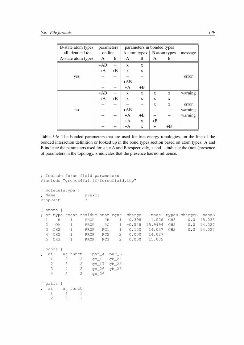
5.8. File formats 149
B-state atom types parameters parameters in bonded typesall identical to on line A atom types B atom types message
A-state atom types A B A B A B+AB − x x+A +B x x
yes − − − − error− − +AB −− − +A +B
+AB − x x x x warning+A +B x x x x− − − − x x error
no − − +AB − − − warning− − +A +B − − warning− − +A x +B −− − +A x + +B
Table 5.6: The bonded parameters that are used for free energy topologies, on the line of thebonded interaction definition or looked up in the bond types section based on atom types. A andB indicate the parameters used for state A and B respectively, + and− indicate the (non-)presenceof parameters in the topology, x indicates that the presence has no influence.
; Include force field parameters#include "gromos43a1.ff/forcefield.itp"
[ moleculetype ]; Name nrexclPropPent 3
[ atoms ]; nr type resnr residue atom cgnr charge mass typeB chargeB massB
1 H 1 PROP PH 1 0.398 1.008 CH3 0.0 15.0352 OA 1 PROP PO 1 -0.548 15.9994 CH2 0.0 14.0273 CH2 1 PROP PC1 1 0.150 14.027 CH2 0.0 14.0274 CH2 1 PROP PC2 2 0.000 14.0275 CH3 1 PROP PC3 2 0.000 15.035
[ bonds ]; ai aj funct par_A par_B
1 2 2 gb_1 gb_262 3 2 gb_17 gb_263 4 2 gb_26 gb_264 5 2 gb_26
[ pairs ]; ai aj funct
1 4 12 5 1

150 Chapter 5. Topologies
[ angles ]; ai aj ak funct par_A par_B
1 2 3 2 ga_11 ga_142 3 4 2 ga_14 ga_143 4 5 2 ga_14 ga_14
[ dihedrals ]; ai aj ak al funct par_A par_B
1 2 3 4 1 gd_12 gd_172 3 4 5 1 gd_17 gd_17
[ system ]; NamePropanol to Pentane
[ molecules ]; Compound #molsPropPent 200
Atoms that are not perturbed, PC2 and PC3, do not need B-state parameter specifications, since theB parameters will be copied from the A parameters. Bonded interactions between atoms that arenot perturbed do not need B parameter specifications, as is the case for the last bond in the exampletopology. Topologies using the OPLS/AA force field need no bonded parameters at all, since boththe A and B parameters are determined by the atom types. Non-bonded interactions involving oneor two perturbed atoms use the free-energy perturbation functional forms. Non-bonded interac-tions between two non-perturbed atoms use the normal functional forms. This means that when,for instance, only the charge of a particle is perturbed, its Lennard-Jones interactions will also beaffected when lambda is not equal to zero or one.
Note that this topology uses the GROMOS-96 force field, in which the bonded interactions are notdetermined by the atom types. The bonded interaction strings are converted by the C-preprocessor.The force-field parameter files contain lines like:
#define gb_26 0.1530 7.1500e+06
#define gd_17 0.000 5.86 3
5.8.5 Constraint forces
The constraint force between two atoms in one molecule can be calculated with the free energyperturbation code by adding a constraint between the two atoms, with a different length in the Aand B topology. When the B length is 1 nm longer than the A length and lambda is kept con-stant at zero, the derivative of the Hamiltonian with respect to lambda is the constraint force. Forconstraints between molecules, the pull code can be used, see sec. 6.4. Below is an example forcalculating the constraint force at 0.7 nm between two methanes in water, by combining the twomethanes into one “molecule.” Note that the definition of a “molecule” in GROMACS does notnecessarily correspond to the chemical definition of a molecule. In GROMACS, a “molecule” can

5.8. File formats 151
be defined as any group of atoms that one wishes to consider simultaneously. The added constraintis of function type 2, which means that it is not used for generating exclusions (see sec. 5.4.4). Notethat the constraint free energy term is included in the derivative term, and is specifically includedin the bonded-lambdas component. However, the free energy for changing constraints is notincluded in the potential energy differences used for BAR and MBAR, as this requires reevaluatingthe energy at each of the constraint components. This functionality is planned for later versions.
; Include force-field parameters#include "gromos43a1.ff/forcefield.itp"
[ moleculetype ]; Name nrexclMethanes 1
[ atoms ]; nr type resnr residu atom cgnr charge mass
1 CH4 1 CH4 C1 1 0 16.0432 CH4 1 CH4 C2 2 0 16.043
[ constraints ]; ai aj funct length_A length_B
1 2 2 0.7 1.7
#include "gromos43a1.ff/spc.itp"
[ system ]; NameMethanes in Water
[ molecules ]; Compound #molsMethanes 1SOL 2002
5.8.6 Coordinate file
Files with the .gro file extension contain a molecular structure in GROMOS-87 format. A samplepiece is included below:
MD of 2 waters, reformat step, PA aug-9161WATER OW1 1 0.126 1.624 1.679 0.1227 -0.0580 0.04341WATER HW2 2 0.190 1.661 1.747 0.8085 0.3191 -0.77911WATER HW3 3 0.177 1.568 1.613 -0.9045 -2.6469 1.31802WATER OW1 4 1.275 0.053 0.622 0.2519 0.3140 -0.17342WATER HW2 5 1.337 0.002 0.680 -1.0641 -1.1349 0.02572WATER HW3 6 1.326 0.120 0.568 1.9427 -0.8216 -0.0244
1.82060 1.82060 1.82060

152 Chapter 5. Topologies
This format is fixed, i.e. all columns are in a fixed position. If you want to read such a file in yourown program without using the GROMACS libraries you can use the following formats:
C-format: "%5i%5s%5s%5i%8.3f%8.3f%8.3f%8.4f%8.4f%8.4f"
Or to be more precise, with title etc. it looks like this:
"%s\n", Title"%5d\n", natomsfor (i=0; (i<natoms); i++)
"%5d%-5s%5s%5d%8.3f%8.3f%8.3f%8.4f%8.4f%8.4f\n",residuenr,residuename,atomname,atomnr,x,y,z,vx,vy,vz
"%10.5f%10.5f%10.5f%10.5f%10.5f%10.5f%10.5f%10.5f%10.5f\n",box[X][X],box[Y][Y],box[Z][Z],box[X][Y],box[X][Z],box[Y][X],box[Y][Z],box[Z][X],box[Z][Y]
Fortran format: (i5,2a5,i5,3f8.3,3f8.4)
So confin.gro is the GROMACS coordinate file and is almost the same as the GROMOS-87file (for GROMOS users: when used with ntx=7). The only difference is the box for whichGROMACS uses a tensor, not a vector.
5.9 Force field organization
5.9.1 Force-field files
Many force fields are available by default. Force fields are detected by the presence of <name>.ffdirectories in the $GMXLIB/share/gromacs/top sub-directory and/or the working direc-tory. The information regarding the location of the force field files is printed by pdb2gmx soyou can easily keep track of which version of a force field is being called, in case you have mademodifications in one location or another. The force fields included with GROMACS are:
• AMBER03 protein, nucleic AMBER94 (Duan et al., J. Comp. Chem. 24, 1999-2012, 2003)
• AMBER94 force field (Cornell et al., JACS 117, 5179-5197, 1995)
• AMBER96 protein, nucleic AMBER94 (Kollman et al., Acc. Chem. Res. 29, 461-469, 1996)
• AMBER99 protein, nucleic AMBER94 (Wang et al., J. Comp. Chem. 21, 1049-1074, 2000)
• AMBER99SB protein, nucleic AMBER94 (Hornak et al., Proteins 65, 712-725, 2006)
• AMBER99SB-ILDN protein, nucleic AMBER94 (Lindorff-Larsen et al., Proteins 78, 1950-58, 2010)
• AMBERGS force field (Garcia & Sanbonmatsu, PNAS 99, 2782-2787, 2002)
• CHARMM27 all-atom force field (CHARM22 plus CMAP for proteins)
• GROMOS96 43a1 force field
• GROMOS96 43a2 force field (improved alkane dihedrals)
• GROMOS96 45a3 force field (Schuler JCC 2001 22 1205)

5.9. Force field organization 153
• GROMOS96 53a5 force field (JCC 2004 vol 25 pag 1656)
• GROMOS96 53a6 force field (JCC 2004 vol 25 pag 1656)
• GROMOS96 54a7 force field (Eur. Biophys. J. (2011), 40„ 843-856, DOI: 10.1007/s00249-011-0700-9)
• OPLS-AA/L all-atom force field (2001 aminoacid dihedrals)
A force field is included at the beginning of a topology file with an #include statement followedby <name>.ff/forcefield.itp. This statement includes the force-field file, which, in turn,may include other force-field files. All the force fields are organized in the same way. An exampleof the amber99.ff/forcefield.itp was shown in 5.8.1.
For each force field, there several files which are only used by pdb2gmx. These are: residuedatabases (.rtp, see 5.7.1) the hydrogen database (.hdb, see 5.7.4), two termini databases(.n.tdb and .c.tdb, see 5.7.5) and the atom type database (.atp, see 5.2.1), which containsonly the masses. Other optional files are described in sec. 5.7.
5.9.2 Changing force-field parameters
If one wants to change the parameters of few bonded interactions in a molecule, this is most easilyaccomplished by typing the parameters behind the definition of the bonded interaction directly inthe *.top file under the [ moleculetype ] section (see 5.8.1 for the format and units). Ifone wants to change the parameters for all instances of a certain interaction one can change themin the force-field file or add a new [ ???types ] section after including the force field. Whenparameters for a certain interaction are defined multiple times, the last definition is used. As ofGROMACS version 3.1.3, a warning is generated when parameters are redefined with a differentvalue. Changing the Lennard-Jones parameters of an atom type is not recommended, because inthe GROMOS force fields the Lennard-Jones parameters for several combinations of atom typesare not generated according to the standard combination rules. Such combinations (and possiblyothers that do follow the combination rules) are defined in the [ nonbond_params ] section,and changing the Lennard-Jones parameters of an atom type has no effect on these combinations.
5.9.3 Adding atom types
As of GROMACS version 3.1.3, atom types can be added in an extra [ atomtypes ] sectionafter the the inclusion of the normal force field. After the definition of the new atom type(s), ad-ditional non-bonded and pair parameters can be defined. In pre-3.1.3 versions of GROMACS, thenew atom types needed to be added in the [ atomtypes ] section of the force-field files, be-cause all non-bonded parameters above the last [ atomtypes ] section would be overwrittenusing the standard combination rules.

154 Chapter 5. Topologies

Chapter 6
Special Topics
6.1 Free energy implementation
For free energy calculations, there are two things that must be specified; the end states, and thepathway connecting the end states. The end states can be specified in two ways. The most straight-forward is through the specification of end states in the topology file. Most potential forms supportboth an A state and a B state. Whenever both states are specified, then the A state corresponds tothe initial free energy state, and the B state corresponds to the final state.
In some cases, the end state can also be defined in some cases without altering the topology,solely through the .mdp file, through the use of the couple-moltype,couple-lambda0,couple-lambda1, and couple-intramol mdp keywords. Any molecule type selected incouple-moltypewill automatically have aB state implicitly constructed (and theA state rede-fined) according to the couple-lambda keywords. couple-lambda0 and couple-lambda1define the non-bonded parameters that are present in the A state (couple-lambda0) and the Bstate (couple-lambda1). The choices are ’q’,’vdw’, and ’vdw-q’; these indicate the Coulom-bic, van der Waals, or both parameters that are turned on in the respective state.
Once the end states are defined, then the path between the end states has to be defined. This pathis defined solely in the .mdp file. Starting in 4.6, λ is a vector of components, with Coulombic,van der Waals, bonded, restraint, and mass components all able to be adjusted independently. Thismakes it possible to turn off the Coulombic term linearly, and then the van der Waals using softcore, all in the same simulation. This is especially useful for replica exchange or expanded en-semble simulations, where it is important to sample all the way from interacting to non-interactingstates in the same simulation to improve sampling.
fep-lambdas is the default array of λ values ranging from 0 to 1. All of the other lambda arraysuse the values in this array if they are not specified. The previous behavior, where the pathwayis controlled by a single λ variable, can be preserved by using only fep-lambdas to define thepathway.
For example, if you wanted to first to change the Coulombic terms, then the van der Waals terms,changing bonded at the same time rate as the van der Waals, but changing the restraints throughout

156 Chapter 6. Special Topics
the first two-thirds of the simulation, then you could use this λ vector:
coul-lambdas = 0.0 0.2 0.5 1.0 1.0 1.0 1.0 1.0 1.0 1.0vdw-lambdas = 0.0 0.0 0.0 0.0 0.4 0.5 0.6 0.7 0.8 1.0bonded-lambdas = 0.0 0.0 0.0 0.0 0.4 0.5 0.6 0.7 0.8 1.0restraint-lambdas = 0.0 0.0 0.1 0.2 0.3 0.5 0.7 1.0 1.0 1.0
This is also equivalent to:
fep-lambdas = 0.0 0.0 0.0 0.0 0.4 0.5 0.6 0.7 0.8 1.0coul-lambdas = 0.0 0.2 0.5 1.0 1.0 1.0 1.0 1.0 1.0 1.0restraint-lambdas = 0.0 0.0 0.1 0.2 0.3 0.5 0.7 1.0 1.0 1.0
The fep-lambda array, in this case, is being used as the default to fill in the bonded and vander Waals λ arrays. Usually, it’s best to fill in all arrays explicitly, just to make sure things areproperly assigned.
If you want to turn on only restraints going from A to B, then it would be:
restraint-lambdas = 0.0 0.1 0.2 0.4 0.6 1.0
and all of the other components of the λ vector would be left in the A state.
To compute free energies with a vector λ using thermodynamic integration, then the TI equationbecomes vector equation:
∆F =
∫〈∇H〉 · d~λ (6.1)
or for finite differences:∆F ≈
∫ ∑〈∇H〉 ·∆λ (6.2)
The external pymbar script downloaded from https://SimTK.org/home/pymbar can compute thisintegral automatically from the GROMACS dhdl.xvg output.
6.2 Potential of mean force
A potential of mean force (PMF) is a potential that is obtained by integrating the mean force froman ensemble of configurations. In GROMACS, there are several different methods to calculate themean force. Each method has its limitations, which are listed below.
• pull code: between the centers of mass of molecules or groups of molecules.
• AWH code: currently acts on coordinates provided by the pull code.
• free-energy code with harmonic bonds or constraints: between single atoms.
• free-energy code with position restraints: changing the conformation of a relatively im-mobile group of atoms.

6.3. Non-equilibrium pulling 157
• pull code in limited cases: between groups of atoms that are part of a larger molecule forwhich the bonds are constrained with SHAKE or LINCS. If the pull group if relatively large,the pull code can be used.
The pull and free-energy code a described in more detail in the following two sections.
Entropic effects
When a distance between two atoms or the centers of mass of two groups is constrained or re-strained, there will be a purely entropic contribution to the PMF due to the rotation of the twogroups [139]. For a system of two non-interacting masses the potential of mean force is:
Vpmf (r) = −(nc − 1)kBT log(r) (6.3)
where nc is the number of dimensions in which the constraint works (i.e. nc = 3 for a normal con-straint and nc = 1 when only the z-direction is constrained). Whether one needs to correct for thiscontribution depends on what the PMF should represent. When one wants to pull a substrate into aprotein, this entropic term indeed contributes to the work to get the substrate into the protein. Butwhen calculating a PMF between two solutes in a solvent, for the purpose of simulating withoutsolvent, the entropic contribution should be removed. Note that this term can be significant; whenat 300K the distance is halved, the contribution is 3.5 kJ mol−1.
6.3 Non-equilibrium pulling
When the distance between two groups is changed continuously, work is applied to the system,which means that the system is no longer in equilibrium. Although in the limit of very slow pullingthe system is again in equilibrium, for many systems this limit is not reachable within reasonablecomputational time. However, one can use the Jarzynski relation [140] to obtain the equilibriumfree-energy difference ∆G between two distances from many non-equilibrium simulations:
∆GAB = −kBT log⟨e−βWAB
⟩A
(6.4)
where WAB is the work performed to force the system along one path from state A to B, theangular bracket denotes averaging over a canonical ensemble of the initial state A and β = 1/kBT .
6.4 The pull code
The pull code applies forces or constraints between the centers of mass of one or more pairs ofgroups of atoms. Each pull reaction coordinate is called a “coordinate” and it operates on usuallytwo, but sometimes more, pull groups. A pull group can be part of one or more pull coordinates.Furthermore, a coordinate can also operate on a single group and an absolute reference position inspace. The distance between a pair of groups can be determined in 1, 2 or 3 dimensions, or canbe along a user-defined vector. The reference distance can be constant or can change linearly withtime. Normally all atoms are weighted by their mass, but an additional weighting factor can alsobe used.
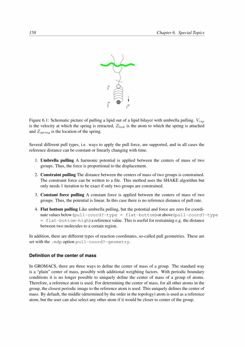
158 Chapter 6. Special Topics
V
zz
linkspring rup
Figure 6.1: Schematic picture of pulling a lipid out of a lipid bilayer with umbrella pulling. Vrupis the velocity at which the spring is retracted, Zlink is the atom to which the spring is attachedand Zspring is the location of the spring.
Several different pull types, i.e. ways to apply the pull force, are supported, and in all cases thereference distance can be constant or linearly changing with time.
1. Umbrella pulling A harmonic potential is applied between the centers of mass of twogroups. Thus, the force is proportional to the displacement.
2. Constraint pulling The distance between the centers of mass of two groups is constrained.The constraint force can be written to a file. This method uses the SHAKE algorithm butonly needs 1 iteration to be exact if only two groups are constrained.
3. Constant force pulling A constant force is applied between the centers of mass of twogroups. Thus, the potential is linear. In this case there is no reference distance of pull rate.
4. Flat bottom pulling Like umbrella pulling, but the potential and force are zero for coordi-nate values below (pull-coord?-type = flat-bottom) or above (pull-coord?-type= flat-bottom-high) a reference value. This is useful for restraining e.g. the distancebetween two molecules to a certain region.
In addition, there are different types of reaction coordinates, so-called pull geometries. These areset with the .mdp option pull-coord?-geometry.
Definition of the center of mass
In GROMACS, there are three ways to define the center of mass of a group. The standard wayis a “plain” center of mass, possibly with additional weighting factors. With periodic boundaryconditions it is no longer possible to uniquely define the center of mass of a group of atoms.Therefore, a reference atom is used. For determining the center of mass, for all other atoms in thegroup, the closest periodic image to the reference atom is used. This uniquely defines the center ofmass. By default, the middle (determined by the order in the topology) atom is used as a referenceatom, but the user can also select any other atom if it would be closer to center of the group.

6.4. The pull code 159
B
Ac.o.m.
a .1
a .2
cd
cd
Figure 6.2: Comparison of a plain center of mass reference group versus a cylinder referencegroup applied to interface systems. C is the reference group. The circles represent the center ofmass of two groups plus the reference group, dc is the reference distance.
For a layered system, for instance a lipid bilayer, it may be of interest to calculate the PMF of alipid as function of its distance from the whole bilayer. The whole bilayer can be taken as referencegroup in that case, but it might also be of interest to define the reaction coordinate for the PMFmore locally. The .mdp option pull-coord?-geometry = cylinder does not use allthe atoms of the reference group, but instead dynamically only those within a cylinder with radiuspull-cylinder-r around the pull vector going through the pull group. This only works fordistances defined in one dimension, and the cylinder is oriented with its long axis along this onedimension. To avoid jumps in the pull force, contributions of atoms are weighted as a function ofdistance (in addition to the mass weighting):
w(r < rcyl) = 1− 2
(r
rcyl
)2
+
(r
rcyl
)4
(6.5)
w(r ≥ rcyl) = 0 (6.6)
Note that the radial dependence on the weight causes a radial force on both cylinder group andthe other pull group. This is an undesirable, but unavoidable effect. To minimize this effect, thecylinder radius should be chosen sufficiently large. The effective mass is 0.47 times that of acylinder with uniform weights and equal to the mass of uniform cylinder of 0.79 times the radius.
For a group of molecules in a periodic system, a plain reference group might not be well-defined.An example is a water slab that is connected periodically in x and y, but has two liquid-vaporinterfaces along z. In such a setup, water molecules can evaporate from the liquid and they willmove through the vapor, through the periodic boundary, to the other interface. Such a system isinherently periodic and there is no proper way of defining a “plain” center of mass along z. Aproper solution is to using a cosine shaped weighting profile for all atoms in the reference group.The profile is a cosine with a single period in the unit cell. Its phase is optimized to give themaximum sum of weights, including mass weighting. This provides a unique and continuousreference position that is nearly identical to the plain center of mass position in case all atoms are

160 Chapter 6. Special Topics
all within a half of the unit-cell length. See ref [141] for details.
When relative weightswi are used during the calculations, either by supplying weights in the inputor due to cylinder geometry or due to cosine weighting, the weights need to be scaled to conservemomentum:
w′i = wi
N∑j=1
wjmj
/N∑j=1
w2j mj (6.7)
where mj is the mass of atom j of the group. The mass of the group, required for calculating theconstraint force, is:
M =N∑i=1
w′imi (6.8)
The definition of the weighted center of mass is:
rcom =N∑i=1
w′imi ri
/M (6.9)
From the centers of mass the AFM, constraint, or umbrella force Fcom on each group can becalculated. The force on the center of mass of a group is redistributed to the atoms as follows:
Fi =w′imi
MFcom (6.10)
Definition of the pull direction
The most common setup is to pull along the direction of the vector containing the two pull groups,this is selected with pull-coord?-geometry = distance. You might want to pull alonga certain vector instead, which is selected with pull-coord?-geometry = direction.But this can cause unwanted torque forces in the system, unless you pull against a reference groupwith (nearly) fixed orientation, e.g. a membrane protein embedded in a membrane along x/y whilepulling along z. If your reference group does not have a fixed orientation, you should probablyuse pull-coord?-geometry = direction-relative, see Fig. 6.3. Since the potentialnow depends on the coordinates of two additional groups defining the orientation, the torque forceswill work on these two groups.
Definition of the angle and dihedral pull geometries
Four pull groups are required for pull-coord?-geometry = angle. In the same wayas for geometries with two groups, each consecutive pair of groups i and i + 1 define a vectorconnecting the COMs of groups i and i + 1. The angle is defined as the angle between the tworesulting vectors. E.g., the .mdp option pull-coord?-groups = 1 2 2 4 defines theangle between the vector from the COM of group 1 to the COM of group 2 and the vector fromthe COM of group 2 to the COM of group 4. The angle takes values in the closed interval [0,180] deg. For pull-coord?-geometry = angle-axis the angle is defined with respectto a reference axis given by pull-coord?-vec and only two groups need to be given. Thedihedral geometry requires six pull groups. These pair up in the same way as described above and
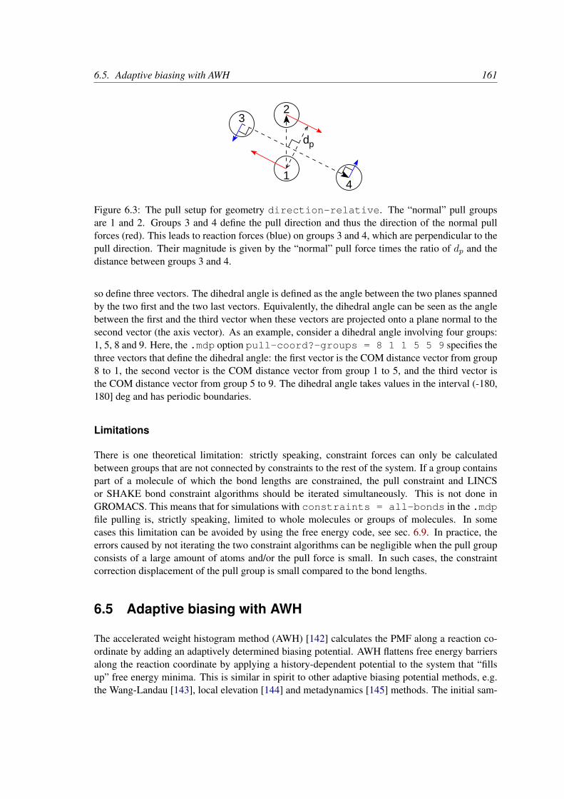
6.5. Adaptive biasing with AWH 161
3
4
dp
2
1
Figure 6.3: The pull setup for geometry direction-relative. The “normal” pull groupsare 1 and 2. Groups 3 and 4 define the pull direction and thus the direction of the normal pullforces (red). This leads to reaction forces (blue) on groups 3 and 4, which are perpendicular to thepull direction. Their magnitude is given by the “normal” pull force times the ratio of dp and thedistance between groups 3 and 4.
so define three vectors. The dihedral angle is defined as the angle between the two planes spannedby the two first and the two last vectors. Equivalently, the dihedral angle can be seen as the anglebetween the first and the third vector when these vectors are projected onto a plane normal to thesecond vector (the axis vector). As an example, consider a dihedral angle involving four groups:1, 5, 8 and 9. Here, the .mdp option pull-coord?-groups = 8 1 1 5 5 9 specifies thethree vectors that define the dihedral angle: the first vector is the COM distance vector from group8 to 1, the second vector is the COM distance vector from group 1 to 5, and the third vector isthe COM distance vector from group 5 to 9. The dihedral angle takes values in the interval (-180,180] deg and has periodic boundaries.
Limitations
There is one theoretical limitation: strictly speaking, constraint forces can only be calculatedbetween groups that are not connected by constraints to the rest of the system. If a group containspart of a molecule of which the bond lengths are constrained, the pull constraint and LINCSor SHAKE bond constraint algorithms should be iterated simultaneously. This is not done inGROMACS. This means that for simulations with constraints = all-bonds in the .mdpfile pulling is, strictly speaking, limited to whole molecules or groups of molecules. In somecases this limitation can be avoided by using the free energy code, see sec. 6.9. In practice, theerrors caused by not iterating the two constraint algorithms can be negligible when the pull groupconsists of a large amount of atoms and/or the pull force is small. In such cases, the constraintcorrection displacement of the pull group is small compared to the bond lengths.
6.5 Adaptive biasing with AWH
The accelerated weight histogram method (AWH) [142] calculates the PMF along a reaction co-ordinate by adding an adaptively determined biasing potential. AWH flattens free energy barriersalong the reaction coordinate by applying a history-dependent potential to the system that “fillsup” free energy minima. This is similar in spirit to other adaptive biasing potential methods, e.g.the Wang-Landau [143], local elevation [144] and metadynamics [145] methods. The initial sam-

162 Chapter 6. Special Topics
pling stage of AWH makes the method robust against the choice of input parameters. Furthermore,the target distribution along the reaction coordinate may be chosen freely.
6.5.1 Basics of the method
Rather than biasing the reaction coordinate ξ(x) directly, AWH acts on a reference coordinate λ.The reaction coordinate ξ(x) is coupled to λ with a harmonic potential
Q(ξ, λ) =1
2βk(ξ − λ)2, (6.11)
so that for large force constants k, ξ ≈ λ. Note the use of dimensionless energies for compatibilitywith previously published work. Units of energy are obtained by multiplication with kBT = 1/β.In the simulation, λ samples the user-defined sampling interval I . For a multidimensional reactioncoordinate ξ, the sampling interval is the Cartesian product I = ΠµIµ (a rectangular domain). Theconnection between atom coordinates and λ is established through the extended ensemble [68],
P (x, λ) =1
Zeg(λ)−Q(ξ(x),λ)−V (x), (6.12)
where g(λ) is a bias function (a free variable) and V (x) is the unbiased potential energy of thesystem. The distribution along λ can be tuned to be any predefined target distribution ρ(λ) (oftenchosen to be flat) by choosing g(λ) wisely. This is evident from
P (λ) =
∫P (x, λ)dx =
1
Zeg(λ)
∫e−Q(ξ(x),λ)−V (x)dx ≡ 1
Zeg(λ)−F (λ), (6.13)
where F (λ) is the free energy
F (λ) = − ln
∫e−Q(ξ(x),λ)−V (x)dx. (6.14)
Being the convolution of the PMF with the Gaussian defined by the harmonic potential, F (λ) isa smoothened version of the PMF. Eq. 6.13 shows that in order to obtain P (λ) = ρ(λ), F (λ)needs to be determined accurately. Thus, AWH adaptively calculates F (λ) and simultaneouslyconverges P (λ) toward ρ(λ).
The free energy update
AWH is initialized with an estimate of the free energyF0(λ). At regular time intervals this estimateis updated using data collected in between the updates. At update n, the applied bias gn(λ) is afunction of the current free energy estimate Fn(λ) and target distribution ρn(λ),
gn(λ) = ln ρn(λ) + Fn(λ), (6.15)
which is consistent with Eq. 6.13. Note that also the target distribution may be updated during thesimulation (see examples in section 6.5.3). Substituting this choice of g = gn back into Eq. 6.13yields the simple free energy update
∆Fn(λ) = F (λ)− Fn(λ) = − lnPn(λ)
ρn(λ), (6.16)

6.5. Adaptive biasing with AWH 163
which would yield a better estimate Fn+1 = Fn + ∆Fn, assuming Pn(λ) can be measured accu-rately. AWH estimates Pn(λ) by regularly calculating the conditional distribution
ωn(λ|x) ≡ Pn(λ|x) =egn(λ)−Q(ξ(x),λ)∑λ′ e
gn(λ′)−Q(ξ(x),λ′). (6.17)
Accumulating these probability weights yields∑t ω(λ|x(t)) ∼ Pn(λ), where
∫Pn(λ|x)Pn(x)dx =
Pn(λ) has been used. The ωn(λ|x) weights are thus the samples of the AWH method. With thelimited amount of sampling one has in practice, update scheme 6.16 yields very noisy results.AWH instead applies a free energy update that has the same form but which can be applied repeat-edly with limited and localized sampling,
∆Fn = − lnWn(λ) +
∑t ωn(λ|x(t))
Wn(λ) +∑t ρn(λ))
. (6.18)
Here Wn(λ) is the reference weight histogram representing prior sampling. The update for W (λ),disregarding the initial stage (see section 6.5.2), is
Wn+1(λ) = Wn(λ) +∑t
ρn(λ). (6.19)
Thus, the weight histogram equals the targeted, “ideal” history of samples. There are two impor-tant things to note about the free energy update. First, sampling is driven away from oversampled,currently local regions. For such λ values, ωn(λ) > ρn(λ) and ∆Fn(λ) < 0, which by Eq. 6.15implies ∆gn(λ) < 0 (assuming ∆ρn ≡ 0). Thus, the probability to sample λ decreases after theupdate (see Eq. 6.13). Secondly, the normalization of the histogramNn =
∑λWn(λ), determines
the update size |∆F (λ)|. For instance, for a single sample ω(λ|x), the shape of the update isapproximately a Gaussian function of width σ = 1/
√βk and height ∝ 1/Nn [142],
|∆Fn(λ)| ∝ 1
Nne−
12βk(ξ(x)−λ)2 . (6.20)
Therefore, as samples accumulate in W (λ) and Nn grows, the updates get smaller, allowing forthe free energy to converge.
Note that quantity of interest to the user is not F (λ) but the PMF Φ(ξ). Φ(ξ) is extracted byreweighting samples ξ(t) on the fly [142] (see also section 6.5.5) and will converge at the samerate as F (λ), see Fig. 6.4. The PMF will be written to output (see section 6.5.7).
Applying the bias to the system
The bias potential can be applied to the system in two ways. Either by applying a harmonicpotential centered at λ(t), which is sampled using (rejection-free) Monte-Carlo sampling fromthe conditional distribution ωn(λ|x(t)) = Pn(λ|x(t)), see Eq. 6.17. This is also called Gibbssampling or independence sampling. Alternatively, and by default in the code, the followingconvolved bias potential can be applied,
Un(ξ) = − ln
∫egn(λ)−Q(ξ,λ)dλ. (6.21)
These two approaches are equivalent in the sense that they give rise to the same biased probabilitiesPn(x) (cf. 6.12) while the dynamics are clearly different in the two cases. This choice does notaffect the internals of the AWH algorithm, only what force and potential AWH returns to the MDengine.

164 Chapter 6. Special Topics
0 Time
Reac
tion co
ordina
te ξ
Initial stage Final stage
ξ(t) Sampling interval
0 Time
Upda
te size 1/N
1/(N0γm )
∼1/t
1/N(t)
0 Time
Log of sam
ple weigh
t, lns
ln(1/γ)
slope∝ln[(N+∆N)/N]
lns(t)
Reaction coordinate ξ
PMF Φ(ξ)
10 k
BT
Exact PMF1st covering2nd3rd
Figure 6.4: AWH evolution in time for a Brownian particle in a double-well potential. The reactioncoordinate ξ(t) traverses the sampling interval multiple times in the initial stage before exitingand entering the final stage (top left). In the final stage, the dynamics of ξ becomes increasinglydiffusive. The times of covering are shown as ×-markers of different colors. At these timesthe free energy update size ∼ 1/N , where N is the size of the weight histogram, is decreased byscalingN by a factor of γ = 3 (top right). In the final stage,N grows at the sampling rate and thus1/N ∼ 1/t. The exit from the final stage is determined on the fly by ensuring that the effectivesample weight s of data collected in the final stage exceeds that of initial stage data (bottom left;note that ln s(t) is plotted). An estimate of the PMF is also extracted from the simulation (bottomright), which after exiting the initial stage should estimate global free energy differences fairlyaccurately.

6.5. Adaptive biasing with AWH 165
6.5.2 The initial stage
Initially, when the bias potential is far from optimal, samples will be highly correlated. In suchcases, letting W (λ) accumulate samples as prescribed by Eq. 6.19, entails a too rapid decay ofthe free energy update size. This motivates splitting the simulation into an initial stage wherethe weight histogram grows according to a more restrictive and robust protocol, and a final stagewhere the the weight histogram grows linearly at the sampling rate (Eq. 6.19). The AWH initialstage takes inspiration from the well-known Wang-Landau algorithm [143], although there aredifferences in the details.
In the initial stage the update size is kept constant (by keeping Nn constant) until a transitionacross the sampling interval has been detected, a “covering”. For the definition of a covering, seeEq. 6.22 below. After a covering has occurred, Nn is scaled up by a constant “growth factor” γ,chosen heuristically as γ = 3. Thus, in the initial stage Nn is set dynamically as Nn = γmN0,where m is the number of coverings. Since the update size scales as 1/N ( Eq. 6.20) this leads toa close to exponential decay of the update size in the initial stage, see Fig. 6.4.
The update size directly determines the rate of change of Fn(λ) and hence, from Eq. 6.15, also therate of change of the bias funcion gn(λ) Thus initially, when Nn is kept small and updates large,the system will be driven along the reaction coordinate by the constantly fluctuating bias. If N0
is set small enough, the first transition will typically be fast because of the large update size andwill quickly give a first rough estimate of the free energy. The second transition, using N1 = γN0
refines this estimate further. Thus, rather than very carefully filling free energy minima using asmall initial update size, the sampling interval is sweeped back-and-forth multiple times, using awide range of update sizes, see Fig. 6.4. This way, the initial stage also makes AWH robust againstthe choice of N0.
The covering criterion
In the general case of a multidimensional reaction coordinate λ = (λµ), the sampling interval I isconsidered covered when all dimensions have been covered. A dimension d is covered if all pointsλµ in the one-dimensional sampling interval Iµ have been “visited”. Finally, a point λµ ∈ Iµhas been visited if there is at least one point λ∗ ∈ I with λ∗µ = λµ that since the last coveringhas accumulated probability weight corresponding to the peak of a multidimensional Gaussiandistribution
∆W (λ∗) ≥ wpeak ≡∏µ
∆λµ√2πσk
. (6.22)
Here, ∆λµ is the point spacing of the discretized Iµ and σk = 1/√βkµ (where kµ is the force
constant) is the Gaussian width.
Exit from the initial stage
For longer times, when major free energy barriers have largely been flattened by the convergingbias potential, the histogram W (λ) should grow at the actual sampling rate and the initial stageneeds to be exited [146]. There are multiple reasonable (heuristic) ways of determining whenthis transition should take place. One option is to postulate that the number of samples in the

166 Chapter 6. Special Topics
weight histogram Nn should never exceed the actual number of collected samples, and exit theinitial stage when this condition breaks [142]. In the initial stage, N grows close to exponentiallywhile the collected number of samples grows linearly, so an exit will surely occur eventually. Herewe instead apply an exit criterion based on the observation that “artifically” keeping N constantwhile continuing to collect samples corresponds to scaling down the relative weight of old samplesrelative to new ones. Similarly, the subsequent scaling up ofN by a factor γ corresponds to scalingup the weight of old data. Briefly, the exit criterion is devised such that the weight of a samplecollected after the initial stage is always larger or equal to the weight of a sample collected duringthe initial stage, see Fig. 6.4. This is consistent with scaling down early, noisy data.
The initial stage exit criterion will now be described in detail. We start out at the beginning of acovering stage, so thatN has just been scaled by γ and is now kept constant. Thus, the first sampleof this stage has the weight s = 1/γ relative to the last sample of the previous covering stage. Weassume that ∆N samples are collected and added to W for each update . To keep N constant, Wneeds to be scaled down by a factor N/(N + ∆N) after every update. Equivalently, this meansthat new data is scaled up relative to old data by the inverse factor. Thus, after ∆n updates a newsample has the relative weight s = (1/γ)[(Nn + ∆N)/Nn]∆n. Now assume covering occurs atthis time. To continue to the next covering stage, N should be scaled by γ, which correspondsto again multiplying s by 1/γ. If at this point s ≥ γ, then after rescaling s ≥ 1; i.e. overall therelative weight of a new sample relative to an old sample is still growing fast. If on the contrarys < γ, and this defines the exit from the initial stage, then the initial stage is over and from now Nsimply grows at the sampling rate (see Eq. 6.19). To really ensure that s ≥ 1 holds before exiting,so that samples after the exit have at least the sample weight of older samples, the last coveringstage is extended by a sufficient number of updates.
6.5.3 Choice of target distribution
The target distribution ρ(λ) is traditionally chosen to be uniform
ρconst(λ) = const. (6.23)
This choice exactly flattens F (λ) in user-defined sampling interval I . Generally, ρ(λ) = 0, λ /∈ I .In certain cases other choices may be preferable. For instance, in the multidimensional case therectangular sampling interval is likely to contain regions of very high free energy, e.g. whereatoms are clashing. To exclude such regions, ρ(λ) can specified by the following function of thefree energy
ρcut(λ) ∝ 1
1 + eF (λ)−Fcut, (6.24)
where Fcut is a free energy cutoff (relative to minλ F (λ)). Thus, regions of the sampling intervalwhere F (λ) > Fcut will be exponentially suppressed (in a smooth fashion). Alternatively, veryhigh free energy regions could be avoided while still flattening more moderate free energy barriersby targeting a Boltzmann distribution corresponding to scaling β = 1/kBT by a factor 0 < sβ <1,
ρBoltz(λ) ∝ e−sβF (λ), (6.25)
The parameter sβ determines to what degree the free energy landscape is flattened; the lower sβ ,the flatter. Note that both ρcut(λ) and ρBoltz(λ) depend on F (λ), which needs to be substituted

6.5. Adaptive biasing with AWH 167
by the current best estimate Fn(λ). Thus, the target distribution is also updated (consistently withEq. 6.15).
There is in fact an alternative approach to obtaining ρBoltz(λ) as the limiting target distributionin AWH, which is particular in the way the weight histogram W (λ) and the target distributionρ are updated and coupled to each other. This yields an evolution of the bias potential which isvery similar to that of well-tempered metadynamics [147], see [142] for details. Because of thepopularity and success of well-tempered metadynamics, this is a special case worth considering.In this case ρ is a function of the reference weight histogram
ρBoltz,loc(λ) ∝W (λ), (6.26)
and the update of the weight histogram is modified (cf. Eq. 6.19)
Wn+1(λ) = Wn(λ) + sβ∑t
ω(λ|x(t)). (6.27)
Thus, here the weight histogram equals the real history of samples, but scaled by sβ . This targetdistribution is called local Boltzmann since W is only modified locally, where sampling has takenplace. We see that when sβ ≈ 0 the histogram essentially does not grow and the size of thefree energy update will stay at a constant value (as in the original formulation of metadynamics).Thus, the free energy estimate will not converge, but continue to fluctuate around the correct value.This illustrates the inherent coupling between the convergence and choice of target distribution forthis special choice of target. Furthermore note that when using ρ = ρBoltz,loc there is no initialstage (section 6.5.2). The rescaling of the weight histogram applied in the initial stage is a globaloperation, which is incompatible ρBoltz,loc only depending locally on the sampling history.
Lastly, the target distribution can be modulated by arbitrary probability weights
ρ(λ) = ρ0(λ)wuser(λ). (6.28)
wherewuser(λ) is provided by user data and in principle ρ0(λ) can be any of the target distributionsmentioned above.
6.5.4 Multiple independent or sharing biases
Multiple independent bias potentials may be applied within one simulation. This only makessense if the biased coordinates ξ(1), ξ(2), . . . evolve essentially independently from one another.A typical example of this would be when applying an independent bias to each monomer of aprotein. Furthermore, multiple AWH simulations can be launched in parallel, each with a (set of)indepedendent biases.
If the defined sampling interval is large relative to the diffusion time of the reaction coordinate,traversing the sampling interval multiple times as is required by the initial stage (section 6.5.2) maytake an infeasible mount of simulation time. In these cases it could be advantageous to parallelizethe work and have a group of multiple “walkers” ξ(i)(t) share a single bias potential. This can beachieved by collecting samples from all ξ(i) of the same sharing group into a single histogram andupdate a common free energy estimate. Samples can be shared between walkers within the simu-lation and/or between multiple simulations. However, currently only sharing between simulationsis supported in the code while all biases within a simulation are independent.
168 Chapter 6. Special Topics
Note that when attempting to shorten the simulation time by using bias-sharing walkers, caremust be taken to ensure the simulations are still long enough to properly explore and equilibrateall regions of the sampling interval. To begin, the walkers in a group should be decorrelatedand distributed approximately according to the target distribution before starting to refine the freeenergy. This can be achieved e.g. by “equilibrating” the shared weight histogram before letting itgrow; for instance, W (λ)/N ≈ ρ(λ) with some tolerance.
Furthermore, the “covering” or transition criterion of the initial stage should to be generalized todetect when the sampling interval has been collectively traversed. One alternative is to just usethe same criterion as for a single walker (but now with more samples), see Eq. 6.22. However, incontrast to the single walker case this does not ensure that any real transitions across the samplinginterval has taken place; in principle all walkers could be sampling only very locally and stillcover the whole interval. Just as with a standard umbrella sampling procedure, the free energymay appear to be converged while in reality simulations sampling closeby λ values are samplingdisconnected regions of phase space. A stricter criterion, which helps avoid such issues, is torequire that before a simulation marks a point λµ along dimension µ as visited, and shares thiswith the other walkers, also all points within a certain diameter Dcover should have been visited(i.e.fulfill Eq. 6.22). Increasing Dcover increases robustness, but may slow down convergence. Forthe maximum value of Dcover, equal to the length of the sampling interval, the sampling intervalis considered covered when at least one walker has independently traversed the sampling interval.
6.5.5 Reweighting and combining biased data
Often one may want to, post-simulation, calculate the unbiased PMF Φ(u) of another variableu(x). Φ(u) can be estimated using ξ-biased data by reweighting (“unbiasing”) the trajectory usingthe bias potential Un(t), see Eq. 6.21. Essentially, one bins the biased data along u and removesthe effect of Un(t) by dividing the weight of samples u(t) by e−Un(t)(ξ(t)),
Φ(u) = − ln∑t
1u(u(t))eUn(t)(ξ(t)Zn(t). (6.29)
Here the indicator function 1u denotes the binning procedure: 1u(u′) = 1 if u′ falls into the binlabeled by u and 0 otherwise. The normalization factor Zn =
∫e−Φ(ξ)−Un(ξ)dξ is the partition
function of the extended ensemble. As can be seen Zn depends on Φ(ξ), the PMF of the (biased)reaction coordinate ξ (which is calculated and written to file by the AWH simulation). It is advis-able to use only final stage data in the reweighting procedure due to the rapid change of the biaspotential during the initial stage. If one would include initial stage data, one should use the sampleweights that are inferred by the repeated rescaling of the histogram in the initial stage, for the sakeof consistency. Initial stage samples would then in any case be heavily scaled down relative to finalstage samples. Note that Eq. 6.29 can also be used to combine data from multiple simulations (byadding another sum also over the trajectory set). Furthermore, when multiple independent AWHbiases have generated a set of PMF estimates Φ(i)(ξ), a combined best estimate Φ(ξ) can beobtained by applying self-consistent exponential averaging. More details on this procedure and aderivation of Eq. 6.29 (using slightly different notation) can be found in [148].

6.5. Adaptive biasing with AWH 169
6.5.6 The friction metric
During the AWH simulation, the following time-integrated force correlation function is calcu-lated,
ηµν(λ) = β
∫ ∞0
〈δFµ(x(t), λ)δFν(x(0), λ)ω(λ|x(t))ω(λ|x(0))〉〈ω2(λ|x)〉
dt. (6.30)
Here Fµ(x, λ) = kµ(ξµ(x) − λµ) is the force along dimension µ from an harmonic potentialcentered at λ and δFµ(x, λ) = Fµ(x, λ) − 〈Fµ(x, λ)〉 is the deviation of the force. The fac-tors ω(λ|x(t)), see Eq. 6.17, reweight the samples. ηµν(λ) is a friction tensor [149]. Its ma-trix elements are inversely proportional to local diffusion coefficients. A measure of sampling(in)efficiency at each λ is given by
η12 (λ) =
√det ηµν(λ). (6.31)
A large value of η12 (λ) indicates slow dynamics and long correlation times, which may require
more sampling.
6.5.7 Usage
AWH stores data in the energy file (.edr) with a frequency set by the user. The data – the PMF,the convolved bias, distributions of the λ and ξ coordinates, etc. – can be extracted after thesimulation using the gmx awh tool. Furthermore, the trajectory of the reaction coordinate ξ(t) isprinted to the pull output file pullx.xvg. The log file (.log) also contains information; checkfor messages starting with “awh”, they will tell you about covering and potential sampling issues.
Setting the initial update size
The initial value of the weight histogram size N sets the initial update size (and the rate of changeof the bias). When N is kept constant, like in the initial stage, the average variance of the freeenergy scales as ε2 ∼ 1/(ND) [142], for a simple model system with constant diffusion D alongthe reaction coordinate. This provides a ballpark estimate used by AWH to initialize N in termsof more meaningful quantities
1
N0=
1
N0(ε0, D)∼ Dε2
0. (6.32)
Essentially, this tells us that a slower system (small D) requires more samples (larger N0) toattain the same level of accuracy (ε0) at a given sampling rate. Conversely, for a system of givendiffusion, how to choose the initial biasing rate depends on how good the initial accuracy is. Boththe initial error ε0 and the diffusionD only need to be roughly estimated or guessed. In the typicalcase, one would only tweak theD parameter, and use a default value for ε0. For good convergence,D should be chosen as large as possible (while maintaining a stable system) giving large initialbias updates and fast initial transitions. ChoosingD too small can lead to slow initial convergence.It may be a good idea to run a short trial simulation and after the first covering check the maximumfree energy difference of the PMF estimate. If this is much larger than the expected magnitude ofthe free energy barriers that should be crossed, then the system is probably being pulled too hardand D should be decreased. ε0 on the other hand, would only be tweaked when starting an AWHsimulation using a fairly accurate guess of the PMF as input.

170 Chapter 6. Special Topics
Tips for efficient sampling
The force constant k should be larger than the curvature of the PMF landscape. If this is notthe case, the distributions of the reaction coordinate ξ and the reference coordinate λ, will differsignificantly and warnings will be printed in the log file. One can choose k as large as the time stepsupports. This will neccessarily increase the number of points of the discretized sampling intervalI . In general however, it should not affect the performance of the simulation noticeably becausethe AWH update is implemented such that only sampled points are accessed at free energy updatetime.
As with any method, the choice of reaction coordinate(s) is critical. If a single reaction coordinatedoes not suffice, identifying a second reaction coordinate and sampling the two-dimensional land-scape may help. In this case, using a target distribution with a free energy cutoff (see Eq. 6.24)might be required to avoid sampling uninteresting regions of very high free energy. Obtainingaccurate free energies for reaction coordinates of much higher dimensionality than 3 or possibly 4is generally not feasible.
Monitoring the transition rate of ξ(t), across the sampling interval is also advisable. For reliablestatistics (e.g. when reweighting the trajectory as described in section 6.5.5), one would generallywant to observe at least a few transitions after having exited the initial stage. Furthermore, ifthe dynamics of the reaction coordinate suddenly changes, this may be a sign of e.g. a reactioncoordinate problem.
Difficult regions of sampling may also be detected by calculating the friction tensor ηµν(λ) inthe sampling interval, see section 6.5.6. ηµν(λ) as well as the sampling efficiency measure η
12 (λ)
(Eq. 6.31) are written to the energy file and can be extracted with gmx awh. A high peak in η12 (λ)
indicates that this region requires longer time to sample properly.
6.6 Enforced Rotation
This module can be used to enforce the rotation of a group of atoms, as e.g. a protein subunit.There are a variety of rotation potentials, among them complex ones that allow flexible adaptationsof both the rotated subunit as well as the local rotation axis during the simulation. An exampleapplication can be found in ref. [150].
6.6.1 Fixed Axis Rotation
Stationary Axis with an Isotropic Potential
In the fixed axis approach (see Fig. 6.5B), torque on a group ofN atoms with positions xi (denoted“rotation group”) is applied by rotating a reference set of atomic positions – usually their initialpositions y0
i – at a constant angular velocity ω around an axis defined by a direction vector v anda pivot point u. To that aim, each atom with position xi is attracted by a “virtual spring” potentialto its moving reference position yi = Ω(t)(y0
i − u), where Ω(t) is a matrix that describes the

6.6. Enforced Rotation 171
Figure 6.5: Comparison of fixed and flexible axis rotation. A: Rotating the sketched shape insidethe white tubular cavity can create artifacts when a fixed rotation axis (dashed) is used. Morerealistically, the shape would revolve like a flexible pipe-cleaner (dotted) inside the bearing (gray).B: Fixed rotation around an axis v with a pivot point specified by the vector u. C: Subdividingthe rotating fragment into slabs with separate rotation axes (↑) and pivot points (•) for each slaballows for flexibility. The distance between two slabs with indices n and n+ 1 is ∆x.
rotation around the axis. In the simplest case, the “springs” are described by a harmonic potential,
V iso =k
2
N∑i=1
wi[Ω(t)(y0
i − u)− (xi − u)]2, (6.33)
with optional mass-weighted prefactors wi = N mi/M with total mass M =∑Ni=1mi. The
rotation matrix Ω(t) is
Ω(t) =
cosωt+ v2x ξ vxvy ξ − vz sinωt vxvz ξ + vy sinωt
vxvy ξ + vz sinωt cosωt+ v2y ξ vyvz ξ − vx sinωt
vxvz ξ − vy sinωt vyvz ξ + vx sinωt cosωt+ v2z ξ
,where vx, vy, and vz are the components of the normalized rotation vector v, and ξ := 1−cos(ωt).As illustrated in Fig. 6.6A for a single atom j, the rotation matrix Ω(t) operates on the initialreference positions y0
j = xj(t0) of atom j at t = t0. At a later time t, the reference position hasrotated away from its initial place (along the blue dashed line), resulting in the force
F isoj = −∇j V iso = k wj
[Ω(t)(y0
j − u)− (xj − u)], (6.34)
which is directed towards the reference position.
Pivot-Free Isotropic Potential
Instead of a fixed pivot vector u this potential uses the center of mass xc of the rotation group aspivot for the rotation axis,
xc =1
M
N∑i=1
mixi and y0c =
1
M
N∑i=1
miy0i , (6.35)

172 Chapter 6. Special Topics
V rm, V flexV iso
V rm2, V flex2 (ε′ = 0.01 nm2)V rm2, V flex2 (ε′ = 0 nm2)
Figure 6.6: Selection of different rotation potentials and definition of notation. All four potentialsV (color coded) are shown for a single atom at position xj(t). A: Isotropic potential V iso, B:radial motion potential V rm and flexible potential V flex, C–D: radial motion 2 potential V rm2
and flexible 2 potential V flex2 for ε′ = 0 nm2 (C) and ε′ = 0.01 nm2 (D). The rotation axis isperpendicular to the plane and marked by ⊗. The light gray contours indicate Boltzmann factorse−V/(kBT ) in the xj-plane for T = 300 K and k = 200 kJ/(mol·nm2). The green arrow showsthe direction of the force Fj acting on atom j; the blue dashed line indicates the motion of thereference position.

6.6. Enforced Rotation 173
which yields the “pivot-free” isotropic potential
V iso-pf =k
2
N∑i=1
wi[Ω(t)(y0
i − y0c)− (xi − xc)
]2, (6.36)
with forcesFiso-pfj = k wj
[Ω(t)(y0
j − y0c)− (xj − xc)
]. (6.37)
Without mass-weighting, the pivot xc is the geometrical center of the group.
Parallel Motion Potential Variant
The forces generated by the isotropic potentials (eqns. 6.33 and 6.36) also contain componentsparallel to the rotation axis and thereby restrain motions along the axis of either the whole ro-tation group (in case of V iso) or within the rotation group (in case of V iso-pf ). For cases whereunrestrained motion along the axis is preferred, we have implemented a “parallel motion” variantby eliminating all components parallel to the rotation axis for the potential. This is achieved byprojecting the distance vectors between reference and actual positions
ri = Ω(t)(y0i − u)− (xi − u) (6.38)
onto the plane perpendicular to the rotation vector,
r⊥i := ri − (ri · v)v , (6.39)
yielding
V pm =k
2
N∑i=1
wi(r⊥i )2
=k
2
N∑i=1
wiΩ(t)(y0
i − u)− (xi − u)
−[
Ω(t)(y0i − u)− (xi − u)
]· vv2, (6.40)
and similarlyF pmj = k wj r
⊥j . (6.41)
Pivot-Free Parallel Motion Potential
Replacing in eqn. 6.40 the fixed pivot u by the center of mass xc yields the pivot-free variant ofthe parallel motion potential. With
si = Ω(t)(y0i − y0
c)− (xi − xc) (6.42)
the respective potential and forces are
V pm-pf =k
2
N∑i=1
wi(s⊥i )2 , (6.43)
F pm-pfj = k wj s
⊥j . (6.44)
174 Chapter 6. Special Topics
Radial Motion Potential
In the above variants, the minimum of the rotation potential is either a single point at the referenceposition yi (for the isotropic potentials) or a single line through yi parallel to the rotation axis (forthe parallel motion potentials). As a result, radial forces restrict radial motions of the atoms. Thetwo subsequent types of rotation potentials, V rm and V rm2, drastically reduce or even eliminatethis effect. The first variant, V rm (Fig. 6.6B), eliminates all force components parallel to the vectorconnecting the reference atom and the rotation axis,
V rm =k
2
N∑i=1
wi [pi · (xi − u)]2 , (6.45)
with
pi :=v ×Ω(t)(y0
i − u)
‖v ×Ω(t)(y0i − u)‖
. (6.46)
This variant depends only on the distance pi · (xi−u) of atom i from the plane spanned by v andΩ(t)(y0
i − u). The resulting force is
Frmj = −k wj
[pj · (xj − u)
]pj . (6.47)
Pivot-Free Radial Motion Potential
Proceeding similar to the pivot-free isotropic potential yields a pivot-free version of the abovepotential. With
qi :=v ×Ω(t)(y0
i − y0c)
‖v ×Ω(t)(y0i − y0
c)‖, (6.48)
the potential and force for the pivot-free variant of the radial motion potential read
V rm-pf =k
2
N∑i=1
wi [qi · (xi − xc)]2 , (6.49)
Frm-pfj = −k wj
[qj · (xj − xc)
]qj + k
mj
M
N∑i=1
wi [qi · (xi − xc)] qi . (6.50)
Radial Motion 2 Alternative Potential
As seen in Fig. 6.6B, the force resulting from V rm still contains a small, second-order radialcomponent. In most cases, this perturbation is tolerable; if not, the following alternative, V rm2,fully eliminates the radial contribution to the force, as depicted in Fig. 6.6C,
V rm2 =k
2
N∑i=1
wi
[(v × (xi − u)) ·Ω(t)(y0
i − u)]2
‖v × (xi − u)‖2 + ε′, (6.51)
where a small parameter ε′ has been introduced to avoid singularities. For ε′ = 0 nm2, the equipo-tential planes are spanned by xi − u and v, yielding a force perpendicular to xi − u, thus notcontracting or expanding structural parts that moved away from or toward the rotation axis.

6.6. Enforced Rotation 175
Choosing a small positive ε′ (e.g., ε′ = 0.01 nm2, Fig. 6.6D) in the denominator of eqn. 6.51 yieldsa well-defined potential and continuous forces also close to the rotation axis, which is not the casefor ε′ = 0 nm2 (Fig. 6.6C). With
ri := Ω(t)(y0i − u) (6.52)
si :=v × (xi − u)
‖v × (xi − u)‖≡ Ψi v × (xi − u) (6.53)
Ψ∗i :=1
‖v × (xi − u)‖2 + ε′(6.54)
the force on atom j reads
F rm2j = −k
wj (sj · rj)
[Ψ∗jΨjrj −
Ψ∗2jΨ3j
(sj · rj)sj
]× v. (6.55)
Pivot-Free Radial Motion 2 Potential
The pivot-free variant of the above potential is
V rm2-pf =k
2
N∑i=1
wi
[(v × (xi − xc)) ·Ω(t)(y0
i − yc)]2
‖v × (xi − xc)‖2 + ε′. (6.56)
With
ri := Ω(t)(y0i − yc) (6.57)
si :=v × (xi − xc)‖v × (xi − xc)‖
≡ Ψi v × (xi − xc) (6.58)
Ψ∗i :=1
‖v × (xi − xc)‖2 + ε′(6.59)
the force on atom j reads
F rm2-pfj = −k
wj (sj · rj)
[Ψ∗jΨjrj −
Ψ∗2jΨ3j
(sj · rj)sj
]× v
+kmj
M
N∑i=1
wi (si · ri)[
Ψ∗iΨiri −
Ψ∗2iΨ3i
(si · ri) si
]× v . (6.60)
6.6.2 Flexible Axis Rotation
As sketched in Fig. 6.5A–B, the rigid body behavior of the fixed axis rotation scheme is a drawbackfor many applications. In particular, deformations of the rotation group are suppressed when theequilibrium atom positions directly depend on the reference positions. To avoid this limitation,eqns. 6.50 and 6.56 will now be generalized towards a “flexible axis” as sketched in Fig. 6.5C. Thiswill be achieved by subdividing the rotation group into a set of equidistant slabs perpendicular tothe rotation vector, and by applying a separate rotation potential to each of these slabs. Fig. 6.5Cshows the midplanes of the slabs as dotted straight lines and the centers as thick black dots.

176 Chapter 6. Special Topics
Figure 6.7: Gaussian functions gn centered at n∆x for a slab distance ∆x = 1.5 nm and n ≥ −2.Gaussian function g0 is highlighted in bold; the dashed line depicts the sum of the shown Gaussianfunctions.
To avoid discontinuities in the potential and in the forces, we define “soft slabs” by weighing thecontributions of each slab n to the total potential function V flex by a Gaussian function
gn(xi) = Γ exp
(−β
2n(xi)
2σ2
), (6.61)
centered at the midplane of the nth slab. Here σ is the width of the Gaussian function, ∆x thedistance between adjacent slabs, and
βn(xi) := xi · v − n∆x . (6.62)
A most convenient choice is σ = 0.7∆x and
1/Γ =∑n∈Z
exp
(−
(n− 14)2
2 · 0.72
)≈ 1.75464 ,
which yields a nearly constant sum, essentially independent of xi (dashed line in Fig. 6.7), i.e.,∑n∈Z
gn(xi) = 1 + ε(xi) , (6.63)
with |ε(xi)| < 1.3 · 10−4. This choice also implies that the individual contributions to the forcefrom the slabs add up to unity such that no further normalization is required.
To each slab center xnc , all atoms contribute by their Gaussian-weighted (optionally also mass-weighted) position vectors gn(xi)xi. The instantaneous slab centers xnc are calculated from thecurrent positions xi,
xnc =
∑Ni=1 gn(xi)mi xi∑Ni=1 gn(xi)mi
, (6.64)
while the reference centers ync are calculated from the reference positions y0i ,
ync =
∑Ni=1 gn(y0
i )mi y0i∑N
i=1 gn(y0i )mi
. (6.65)
Due to the rapid decay of gn, each slab will essentially involve contributions from atoms locatedwithin ≈ 3∆x from the slab center only.

6.6. Enforced Rotation 177
Flexible Axis Potential
We consider two flexible axis variants. For the first variant, the slab segmentation procedure withGaussian weighting is applied to the radial motion potential (eqn. 6.50 / Fig. 6.6B), yielding as thecontribution of slab n
V n =k
2
N∑i=1
wi gn(xi) [qni · (xi − xnc )]2 ,
and a total potential function
V flex =∑n
V n . (6.66)
Note that the global center of mass xc used in eqn. 6.50 is now replaced by xnc , the center of massof the slab. With
qni :=v ×Ω(t)(y0
i − ync )
‖v ×Ω(t)(y0i − ync )‖
(6.67)
bni := qni · (xi − xnc ) , (6.68)
the resulting force on atom j reads
F flexj = − k wj
∑n
gn(xj) bnj
qnj − bnj
βn(xj)
2σ2v
+ kmj
∑n
gn(xj)∑h gn(xh)
N∑i=1
wi gn(xi) bni
qni −
βn(xj)
σ2[qni · (xj − xnc )] v
. (6.69)
Note that for V flex, as defined, the slabs are fixed in space and so are the reference centers ync . Ifduring the simulation the rotation group moves too far in v direction, it may enter a region where– due to the lack of nearby reference positions – no reference slab centers are defined, renderingthe potential evaluation impossible. We therefore have included a slightly modified version ofthis potential that avoids this problem by attaching the midplane of slab n = 0 to the center ofmass of the rotation group, yielding slabs that move with the rotation group. This is achieved bysubtracting the center of mass xc of the group from the positions,
xi = xi − xc , and y0i = y0
i − y0c , (6.70)
such that
V flex-t =k
2
∑n
N∑i=1
wi gn(xi)
[v ×Ω(t)(y0
i − ync )
‖v ×Ω(t)(y0i − ync )‖
· (xi − xnc )
]2
. (6.71)
To simplify the force derivation, and for efficiency reasons, we here assume xc to be constant, andthus ∂xc/∂x = ∂xc/∂y = ∂xc/∂z = 0. The resulting force error is small (of order O(1/N) orO(mj/M) if mass-weighting is applied) and can therefore be tolerated. With this assumption, theforces F flex-t have the same form as eqn. 6.69.

178 Chapter 6. Special Topics
Flexible Axis 2 Alternative Potential
In this second variant, slab segmentation is applied to V rm2 (eqn. 6.56), resulting in a flexible axispotential without radial force contributions (Fig. 6.6C),
V flex2 =k
2
N∑i=1
∑n
wi gn(xi)
[(v × (xi − xnc )) ·Ω(t)(y0
i − ync )]2
‖v × (xi − xnc )‖2 + ε′. (6.72)
With
rni := Ω(t)(y0i − ync ) (6.73)
sni :=v × (xi − xnc )
‖v × (xi − xnc )‖≡ ψi v × (xi − xnc ) (6.74)
ψ∗i :=1
‖v × (xi − xnc )‖2 + ε′(6.75)
Wnj :=
gn(xj)mj∑h gn(xh)mh
(6.76)
Sn :=N∑i=1
wi gn(xi) (sni · rni )
[ψ∗iψirni −
ψ∗2iψ3i
(sni · rni ) sni
](6.77)
the force on atom j reads
F flex2j = −k
∑n
wj gn(xj) (snj · rnj )
[ψ∗jψjrnj −
ψ∗2jψ3j
(snj · rnj ) snj
]× v
+k
∑n
Wnj S
n
× v − k
∑n
Wnj
βn(xj)
σ2
1
ψjsnj · Sn
v
+k
2
∑n
wj gn(xj)βn(xj)
σ2
ψ∗jψ2j
(snj · rnj )2
v. (6.78)
Applying transformation (6.70) yields a “translation-tolerant” version of the flexible 2 potential,V flex2-t. Again, assuming that ∂xc/∂x, ∂xc/∂y, ∂xc/∂z are small, the resulting equations forV flex2-t and F flex2-t are similar to those of V flex2 and F flex2.
6.6.3 Usage
To apply enforced rotation, the particles i that are to be subjected to one of the rotation potentialsare defined via index groups rot-group0, rot-group1, etc., in the .mdp input file. Thereference positions y0
i are read from a special .trr file provided to grompp. If no such file isfound, xi(t = 0) are used as reference positions and written to .trr such that they can be used forsubsequent setups. All parameters of the potentials such as k, ε′, etc. (Table 6.1) are provided as.mdp parameters; rot-type selects the type of the potential. The option rot-massw allowsto choose whether or not to use mass-weighted averaging. For the flexible potentials, a cutoffvalue gmin
n (typically gminn = 0.001) makes shure that only significant contributions to V and F
are evaluated, i.e. terms with gn(x) < gminn are omitted. Table 6.2 summarizes observables that
are written to additional output files and which are described below.

6.6. Enforced Rotation 179
Table 6.1: Parameters used by the various rotation potentials. x’s indicate which parameter isactually used for a given potential.
parameter k v u ω ε′ ∆x gminn
.mdp input variable name k vec pivot rate eps slab-dist min-gaussunit kJ
mol·nm2 - nm /ps nm2 nm -
fixed axis potentials: eqn.isotropic V iso (6.33) x x x x - - -— pivot-free V iso-pf (6.36) x x - x - - -parallel motion V pm (6.40) x x x x - - -— pivot-free V pm-pf (6.44) x x - x - - -radial motion V rm (6.45) x x x x - - -— pivot-free V rm-pf (6.50) x x - x - - -radial motion 2 V rm2 (6.51) x x x x x - -— pivot-free V rm2-pf (6.56) x x - x x - -flexible axis potentials: eqn.flexible V flex (6.66) x x - x - x x— transl. tol. V flex-t (6.71) x x - x - x xflexible 2 V flex2 (6.72) x x - x x x x— transl. tol. V flex2-t - x x - x x x x
Table 6.2: Quantities recorded in output files during enforced rotation simulations. All slab-wisedata is written every nstsout steps, other rotation data every nstrout steps.
quantity unit equation output file fixed flexibleV (t) kJ/mol see 6.1 rotation x xθref(t) degrees θref(t) = ωt rotation x xθav(t) degrees (6.79) rotation x -θfit(t), θfit(t, n) degrees (6.81) rotangles - xy0(n), x0(t, n) nm (6.64, 6.65) rotslabs - xτ(t) kJ/mol (6.82) rotation x -τ(t, n) kJ/mol (6.82) rottorque - x
180 Chapter 6. Special Topics
Angle of Rotation Groups: Fixed Axis
For fixed axis rotation, the average angle θav(t) of the group relative to the reference group isdetermined via the distance-weighted angular deviation of all rotation group atoms from theirreference positions,
θav =N∑i=1
ri θi
/N∑i=1
ri . (6.79)
Here, ri is the distance of the reference position to the rotation axis, and the difference angles θiare determined from the atomic positions, projected onto a plane perpendicular to the rotation axisthrough pivot point u (see eqn. 6.39 for the definition of ⊥),
cos θi =(yi − u)⊥ · (xi − u)⊥
‖(yi − u)⊥ · (xi − u)⊥‖. (6.80)
The sign of θav is chosen such that θav > 0 if the actual structure rotates ahead of the reference.
Angle of Rotation Groups: Flexible Axis
For flexible axis rotation, two outputs are provided, the angle of the entire rotation group, andseparate angles for the segments in the slabs. The angle of the entire rotation group is determinedby an RMSD fit of xi to the reference positions y0
i at t = 0, yielding θfit as the angle by whichthe reference has to be rotated around v for the optimal fit,
RMSD(xi, Ω(θfit)y0i )
!= min . (6.81)
To determine the local angle for each slab n, both reference and actual positions are weighted withthe Gaussian function of slab n, and θfit(t, n) is calculated as in eqn. 6.81) from the Gaussian-weighted positions.
For all angles, the .mdp input option rot-fit-method controls whether a normal RMSD fitis performed or whether for the fit each position xi is put at the same distance to the rotation axisas its reference counterpart y0
i . In the latter case, the RMSD measures only angular differences,not radial ones.
Angle Determination by Searching the Energy Minimum
Alternatively, for rot-fit-method = potential, the angle of the rotation group is deter-mined as the angle for which the rotation potential energy is minimal. Therefore, the used rotationpotential is additionally evaluated for a set of angles around the current reference angle. In thiscase, the rotangles.log output file contains the values of the rotation potential at the chosenset of angles, while rotation.xvg lists the angle with minimal potential energy.
Torque
The torque τ (t) exerted by the rotation potential is calculated for fixed axis rotation via
τ (t) =N∑i=1
ri(t)× f⊥i (t), (6.82)

6.7. Electric fields 181
where ri(t) is the distance vector from the rotation axis to xi(t) and f⊥i (t) is the force componentperpendicular to ri(t) and v. For flexible axis rotation, torques τn are calculated for each slabusing the local rotation axis of the slab and the Gaussian-weighted positions.
6.7 Electric fields
A pulsed and oscillating electric field can be applied according to:
E(t) = E0 exp
[−(t− t0)2
2σ2
]cos [ω(t− t0)] (6.83)
where E0 is the field strength, the angular frequency ω = 2πc/λ, t0 is the time at of the peak inthe field strength and σ is the with of the pulse. Special cases occur when σ = 0 (non-pulsed field)and for ω is 0 (static field).
This simulated laser-pulse was applied to simulations of melting ice [151]. A pulsed electric fieldmay look ike Fig. 6.8. In the supporting information of that paper the impact of an applied electricfield on a system under periodic boundary conditions is analyzed. It is described that the effectiveelectric field under PBC is larger than the applied field, by a factor depending on the size of the boxand the dielectric properties of molecules in the box. For a system with static dielectric propertiesthis factor can be corrected for. But for a system where the dielectric varies over time, for examplea membrane protein with a pore that opens and closes during the simulatippn, this way of applyingan electric field is not useful. In such cases one can use the computational electrophysiologyprotocol described in the next section (sec. 6.8).
0 0.5 1 1.5 2Time (ps)
-2
-1
0
1
2
Ele
ctr
ic fie
ld (
V/n
m)
Figure 6.8: A simulated laser pulse in GROMACS.
Electric fields are applied when the following options are specified in the grompp.mdp file. Youspecify, in order, E0, ω, t0 and σ:
electric-field-x = 0.04 0 0 0
yields a static field with E0 = 0.04 V/nm in the X-direction. In contrast,

182 Chapter 6. Special Topics
electric-field-x = 2.0 150 5 0
yields an oscillating electric field with E0 = 2 V/nm, ω = 150/ps and t0 = 5 ps. Finally
electric-field-x = 2.0 150 5 1
yields an pulsed-oscillating electric field with E0 = 2 V/nm, ω = 150/ps and t0 = 5 ps and σ = 1 ps.Read more in ref. [151]. Note that the input file format is changed from the undocumented olderversion. A figure like Fig. 6.8 may be produced by passing the -field option to gmx mdrun.
6.8 Computational Electrophysiology
The Computational Electrophysiology (CompEL) protocol [152] allows the simulation of ion fluxthrough membrane channels, driven by transmembrane potentials or ion concentration gradients.Just as in real cells, CompEL establishes transmembrane potentials by sustaining a small imbal-ance of charges ∆q across the membrane, which gives rise to a potential difference ∆U accordingto the membrane capacitance:
∆U = ∆q/Cmembrane (6.84)
The transmembrane electric field and concentration gradients are controlled by .mdp options,which allow the user to set reference counts for the ions on either side of the membrane. If a dif-ference between the actual and the reference numbers persists over a certain time span, specifiedby the user, a number of ion/water pairs are exchanged between the compartments until the refer-ence numbers are restored. Alongside the calculation of channel conductance and ion selectivity,CompEL simulations also enable determination of the channel reversal potential, an importantcharacteristic obtained in electrophysiology experiments.
In a CompEL setup, the simulation system is divided into two compartments A and B with inde-pendent ion concentrations. This is best achieved by using double bilayer systems with a copy (orcopies) of the channel/pore of interest in each bilayer (Fig. 6.9 A, B). If the channel axes point inthe same direction, channel flux is observed simultaneously at positive and negative potentials inthis way, which is for instance important for studying channel rectification.
The potential difference ∆U across the membrane is easily calculated with the gmx potentialutility. By this, the potential drop along z or the pore axis is exactly known in each time intervalof the simulation (Fig. 6.9 C). Type and number of ions ni of charge qi, traversing the channel inthe simulation, are written to the swapions.xvg output file, from which the average channelconductance G in each interval ∆t is determined by:
G =
∑i niqi
∆t∆U. (6.85)
The ion selectivity is calculated as the number flux ratio of different species. Best results areobtained by averaging these values over several overlapping time intervals.
The calculation of reversal potentials is best achieved using a small set of simulations in whicha given transmembrane concentration gradient is complemented with small ion imbalances ofvarying magnitude. For example, if one compartment contains 1 M salt and the other 0.1 M, and
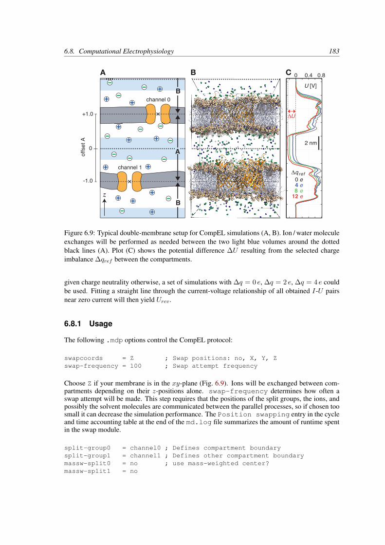
6.8. Computational Electrophysiology 183
B
B
A B CU [V]
z
A
0 0.4 0.8
2 nm
qref
4 e8 e
12 e
0 e
U
channel 1
channel 0
0
+1.0
-1.0
offs
et A
Figure 6.9: Typical double-membrane setup for CompEL simulations (A, B). Ion / water moleculeexchanges will be performed as needed between the two light blue volumes around the dottedblack lines (A). Plot (C) shows the potential difference ∆U resulting from the selected chargeimbalance ∆qref between the compartments.
given charge neutrality otherwise, a set of simulations with ∆q = 0 e, ∆q = 2 e, ∆q = 4 e couldbe used. Fitting a straight line through the current-voltage relationship of all obtained I-U pairsnear zero current will then yield Urev.
6.8.1 Usage
The following .mdp options control the CompEL protocol:
swapcoords = Z ; Swap positions: no, X, Y, Zswap-frequency = 100 ; Swap attempt frequency
Choose Z if your membrane is in the xy-plane (Fig. 6.9). Ions will be exchanged between com-partments depending on their z-positions alone. swap-frequency determines how often aswap attempt will be made. This step requires that the positions of the split groups, the ions, andpossibly the solvent molecules are communicated between the parallel processes, so if chosen toosmall it can decrease the simulation performance. The Position swapping entry in the cycleand time accounting table at the end of the md.log file summarizes the amount of runtime spentin the swap module.
split-group0 = channel0 ; Defines compartment boundarysplit-group1 = channel1 ; Defines other compartment boundarymassw-split0 = no ; use mass-weighted center?massw-split1 = no

184 Chapter 6. Special Topics
split-group0 and split-group1 are two index groups that define the boundaries betweenthe two compartments, which are usually the centers of the channels. If massw-split0 ormassw-split1 are set to yes, the center of mass of each index group is used as boundary, herein z-direction. Otherwise, the geometrical centers will be used (× in Fig. 6.9 A). If, such as here,a membrane channel is selected as split group, the center of the channel will define the dividingplane between the compartments (dashed horizontal lines). All index groups must be defined inthe index file.
If, to restore the requested ion counts, an ion from one compartment has to be exchanged with awater molecule from the other compartment, then those molecules are swapped which have thelargest distance to the compartment-defining boundaries (dashed horizontal lines). Depending onthe ion concentration, this effectively results in exchanges of molecules between the light bluevolumes. If a channel is very asymmetric in z-direction and would extend into one of the swapvolumes, one can offset the swap exchange plane with the bulk-offset parameter. A valueof 0.0 means no offset b, values −1.0 < b < 0 move the swap exchange plane closer to thelower, values 0 < b < 1.0 closer to the upper membrane. Fig. 6.9 A (left) depicts that for the Acompartment.
solvent-group = SOL ; Group containing the solvent moleculesiontypes = 3 ; Number of different ion types to controliontype0-name = NA ; Group name of the ion typeiontype0-in-A = 51 ; Reference count of ions of type 0 in Aiontype0-in-B = 35 ; Reference count of ions of type 0 in Biontype1-name = Kiontype1-in-A = 10iontype1-in-B = 38iontype2-name = CLiontype2-in-A = -1iontype2-in-B = -1
The group name of solvent molecules acting as exchange partners for the ions has to be set withsolvent-group. The number of different ionic species under control of the CompEL protocolis given by the iontypes parameter, while iontype0-name gives the name of the indexgroup containing the atoms of this ionic species. The reference number of ions of this type canbe set with the iontype0-in-A and iontype0-in-B options for compartments A and B,respectively. Obviously, the sum of iontype0-in-A and iontype0-in-B needs to equalthe number of ions in the group defined by iontype0-name. A reference number of -1 means:use the number of ions as found at the beginning of the simulation as the reference value.
coupl-steps = 10 ; Average over these many swap stepsthreshold = 1 ; Do not swap if < threshold
If coupl-steps is set to 1, then the momentary ion distribution determines whether ions areexchanged. coupl-steps > 1 will use the time-average of ion distributions over the selectednumber of attempt steps instead. This can be useful, for example, when ions diffuse near compart-ment boundaries, which would lead to numerous unproductive ion exchanges. A threshold of1 means that a swap is performed if the average ion count in a compartment differs by at least 1

6.9. Calculating a PMF using the free-energy code 185
from the requested values. Higher thresholds will lead to toleration of larger differences. Ions areexchanged until the requested number ± the threshold is reached.
cyl0-r = 5.0 ; Split cylinder 0 radius (nm)cyl0-up = 0.75 ; Split cylinder 0 upper extension (nm)cyl0-down = 0.75 ; Split cylinder 0 lower extension (nm)cyl1-r = 5.0 ; same for other channelcyl1-up = 0.75cyl1-down = 0.75
The cylinder options are used to define virtual geometric cylinders around the channel’s pore totrack how many ions of which type have passed each channel. Ions will be counted as havingtraveled through a channel according to the definition of the channel’s cylinder radius, upper andlower extension, relative to the location of the respective split group. This will not affect theactual flux or exchange, but will provide you with the ion permeation numbers across each of thechannels. Note that an ion can only be counted as passing through a particular channel if it isdetected within the defined split cylinder in a swap step. If swap-frequency is chosen toohigh, a particular ion may be detected in compartment A in one swap step, and in compartment Bin the following swap step, so it will be unclear through which of the channels it has passed.
A double-layered system for CompEL simulations can be easily prepared by duplicating an exist-ing membrane/channel MD system in the direction of the membrane normal (typically z) with gmxeditconf -translate 0 0 <l_z>, where l_z is the box length in that direction. If youhave already defined index groups for the channel for the single-layered system, gmx make_ndx-n index.ndx -twin will provide you with the groups for the double-layered system.
To suppress large fluctuations of the membranes along the swap direction, it may be useful toapply a harmonic potential (acting only in the swap dimension) between each of the two channeland/or bilayer centers using umbrella pulling (see section 6.4).
Multimeric channels
If a split group consists of more than one molecule, the correct PBC image of all molecules withrespect to each other has to be chosen such that the channel center can be correctly determined.GROMACS assumes that the starting structure in the .tpr file has the correct PBC representation.Set the following environment variable to check whether that is the case:
• GMX_COMPELDUMP: output the starting structure after it has been made whole to .pdbfile.
6.9 Calculating a PMF using the free-energy code
The free-energy coupling-parameter approach (see sec. 3.12) provides several ways to calculatepotentials of mean force. A potential of mean force between two atoms can be calculated byconnecting them with a harmonic potential or a constraint. For this purpose there are specialpotentials that avoid the generation of extra exclusions, see sec. 5.4.4. When the position of the

186 Chapter 6. Special Topics
minimum or the constraint length is 1 nm more in state B than in state A, the restraint or constraintforce is given by ∂H/∂λ. The distance between the atoms can be changed as a function of λ andtime by setting delta-lambda in the .mdp file. The results should be identical (although notnumerically due to the different implementations) to the results of the pull code with umbrellasampling and constraint pulling. Unlike the pull code, the free energy code can also handle atomsthat are connected by constraints.
Potentials of mean force can also be calculated using position restraints. With position restraints,atoms can be linked to a position in space with a harmonic potential (see 4.3.1). These positionscan be made a function of the coupling parameter λ. The positions for the A and the B states aresupplied to grompp with the -r and -rb options, respectively. One could use this approach todo targeted MD; note that we do not encourage the use of targeted MD for proteins. A proteincan be forced from one conformation to another by using these conformations as position restraintcoordinates for state A and B. One can then slowly change λ from 0 to 1. The main drawback ofthis approach is that the conformational freedom of the protein is severely limited by the positionrestraints, independent of the change from state A to B. Also, the protein is forced from state A toB in an almost straight line, whereas the real pathway might be very different. An example of amore fruitful application is a solid system or a liquid confined between walls where one wants tomeasure the force required to change the separation between the boundaries or walls. Because theboundaries (or walls) already need to be fixed, the position restraints do not limit the system in itssampling.
6.10 Removing fastest degrees of freedom
The maximum time step in MD simulations is limited by the smallest oscillation period that canbe found in the simulated system. Bond-stretching vibrations are in their quantum-mechanicalground state and are therefore better represented by a constraint instead of a harmonic potential.
For the remaining degrees of freedom, the shortest oscillation period (as measured from a simu-lation) is 13 fs for bond-angle vibrations involving hydrogen atoms. Taking as a guideline thatwith a Verlet (leap-frog) integration scheme a minimum of 5 numerical integration steps should beperformed per period of a harmonic oscillation in order to integrate it with reasonable accuracy,the maximum time step will be about 3 fs. Disregarding these very fast oscillations of period 13 fs,the next shortest periods are around 20 fs, which will allow a maximum time step of about 4 fs.
Removing the bond-angle degrees of freedom from hydrogen atoms can best be done by definingthem as virtual interaction sites instead of normal atoms. Whereas a normal atom is connectedto the molecule with bonds, angles and dihedrals, a virtual site’s position is calculated from theposition of three nearby heavy atoms in a predefined manner (see also sec. 4.7). For the hydrogensin water and in hydroxyl, sulfhydryl, or amine groups, no degrees of freedom can be removed,because rotational freedom should be preserved. The only other option available to slow downthese motions is to increase the mass of the hydrogen atoms at the expense of the mass of theconnected heavy atom. This will increase the moment of inertia of the water molecules and thehydroxyl, sulfhydryl, or amine groups, without affecting the equilibrium properties of the systemand without affecting the dynamical properties too much. These constructions will shortly bedescribed in sec. 6.10.1 and have previously been described in full detail [153].
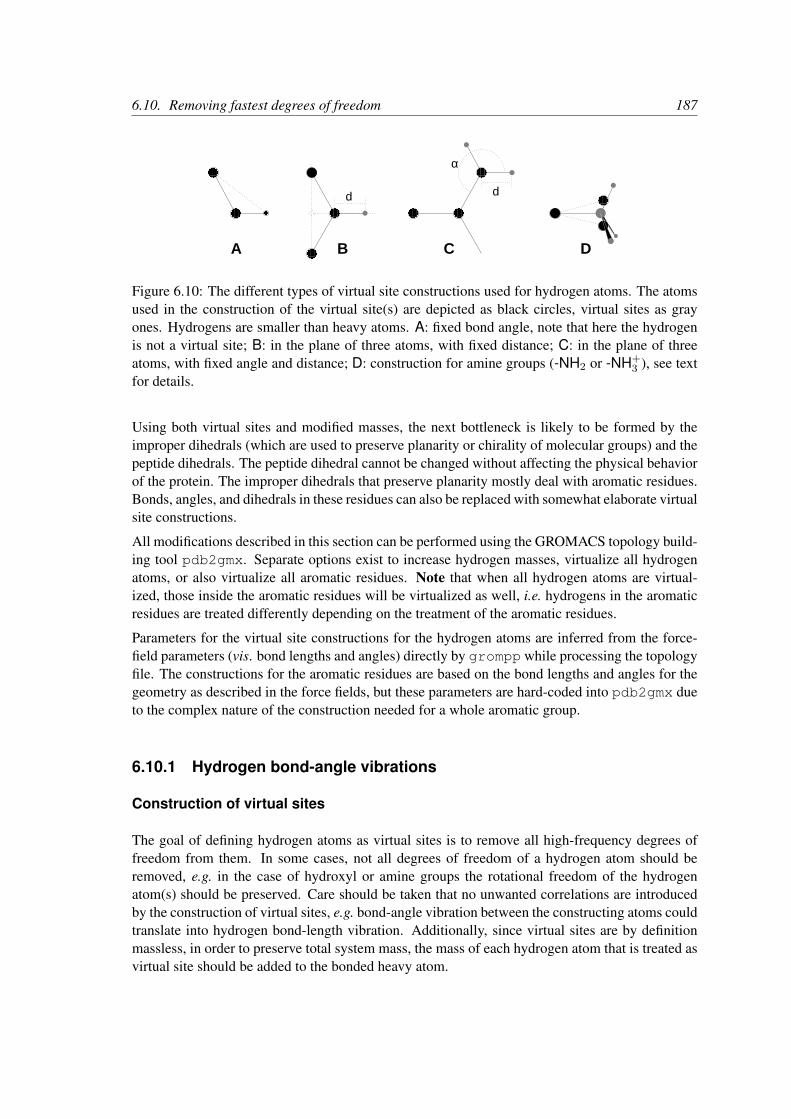
6.10. Removing fastest degrees of freedom 187
D
d
α
d
BA C
Figure 6.10: The different types of virtual site constructions used for hydrogen atoms. The atomsused in the construction of the virtual site(s) are depicted as black circles, virtual sites as grayones. Hydrogens are smaller than heavy atoms. A: fixed bond angle, note that here the hydrogenis not a virtual site; B: in the plane of three atoms, with fixed distance; C: in the plane of threeatoms, with fixed angle and distance; D: construction for amine groups (-NH2 or -NH+
3 ), see textfor details.
Using both virtual sites and modified masses, the next bottleneck is likely to be formed by theimproper dihedrals (which are used to preserve planarity or chirality of molecular groups) and thepeptide dihedrals. The peptide dihedral cannot be changed without affecting the physical behaviorof the protein. The improper dihedrals that preserve planarity mostly deal with aromatic residues.Bonds, angles, and dihedrals in these residues can also be replaced with somewhat elaborate virtualsite constructions.
All modifications described in this section can be performed using the GROMACS topology build-ing tool pdb2gmx. Separate options exist to increase hydrogen masses, virtualize all hydrogenatoms, or also virtualize all aromatic residues. Note that when all hydrogen atoms are virtual-ized, those inside the aromatic residues will be virtualized as well, i.e. hydrogens in the aromaticresidues are treated differently depending on the treatment of the aromatic residues.
Parameters for the virtual site constructions for the hydrogen atoms are inferred from the force-field parameters (vis. bond lengths and angles) directly by grompp while processing the topologyfile. The constructions for the aromatic residues are based on the bond lengths and angles for thegeometry as described in the force fields, but these parameters are hard-coded into pdb2gmx dueto the complex nature of the construction needed for a whole aromatic group.
6.10.1 Hydrogen bond-angle vibrations
Construction of virtual sites
The goal of defining hydrogen atoms as virtual sites is to remove all high-frequency degrees offreedom from them. In some cases, not all degrees of freedom of a hydrogen atom should beremoved, e.g. in the case of hydroxyl or amine groups the rotational freedom of the hydrogenatom(s) should be preserved. Care should be taken that no unwanted correlations are introducedby the construction of virtual sites, e.g. bond-angle vibration between the constructing atoms couldtranslate into hydrogen bond-length vibration. Additionally, since virtual sites are by definitionmassless, in order to preserve total system mass, the mass of each hydrogen atom that is treated asvirtual site should be added to the bonded heavy atom.

188 Chapter 6. Special Topics
ε
η
ζδ
ε
γ
ε
δ ε
δ
εδ
γ
ζε
η
εδ
γ
Phe Tyr HisTrp
ζ
ε
ζ
εδ
γ
δδ
Figure 6.11: The different types of virtual site constructions used for aromatic residues. The atomsused in the construction of the virtual site(s) are depicted as black circles, virtual sites as gray ones.Hydrogens are smaller than heavy atoms. A: phenylalanine; B: tyrosine (note that the hydroxylhydrogen is not a virtual site); C: tryptophan; D: histidine.
Taking into account these considerations, the hydrogen atoms in a protein naturally fall into severalcategories, each requiring a different approach (see also Fig. 6.10).
• hydroxyl (-OH) or sulfhydryl (-SH) hydrogen: The only internal degree of freedom in ahydroxyl group that can be constrained is the bending of the C-O-H angle. This angle isfixed by defining an additional bond of appropriate length, see Fig. 6.10A. Doing so removesthe high-frequency angle bending, but leaves the dihedral rotational freedom. The same goesfor a sulfhydryl group. Note that in these cases the hydrogen is not treated as a virtual site.
• single amine or amide (-NH-) and aromatic hydrogens (-CH-): The position of these hy-drogens cannot be constructed from a linear combination of bond vectors, because of theflexibility of the angle between the heavy atoms. Instead, the hydrogen atom is positionedat a fixed distance from the bonded heavy atom on a line going through the bonded heavyatom and a point on the line through both second bonded atoms, see Fig. 6.10B.
• planar amine (-NH2) hydrogens: The method used for the single amide hydrogen is not wellsuited for planar amine groups, because no suitable two heavy atoms can be found to definethe direction of the hydrogen atoms. Instead, the hydrogen is constructed at a fixed distancefrom the nitrogen atom, with a fixed angle to the carbon atom, in the plane defined by oneof the other heavy atoms, see Fig. 6.10C.
• amine group (umbrella -NH2 or -NH+3 ) hydrogens: Amine hydrogens with rotational free-
dom cannot be constructed as virtual sites from the heavy atoms they are connected to, sincethis would result in loss of the rotational freedom of the amine group. To preserve the rota-tional freedom while removing the hydrogen bond-angle degrees of freedom, two “dummymasses” are constructed with the same total mass, moment of inertia (for rotation aroundthe C-N bond) and center of mass as the amine group. These dummy masses have no in-teraction with any other atom, except for the fact that they are connected to the carbon andto each other, resulting in a rigid triangle. From these three particles, the positions of thenitrogen and hydrogen atoms are constructed as linear combinations of the two carbon-massvectors and their outer product, resulting in an amine group with rotational freedom intact,but without other internal degrees of freedom. See Fig. 6.10D.

6.11. Viscosity calculation 189
6.10.2 Out-of-plane vibrations in aromatic groups
The planar arrangements in the side chains of the aromatic residues lends itself perfectly to avirtual-site construction, giving a perfectly planar group without the inherently unstable con-straints that are necessary to keep normal atoms in a plane. The basic approach is to define threeatoms or dummy masses with constraints between them to fix the geometry and create the rest ofthe atoms as simple virtual sites type (see sec. 4.7) from these three. Each of the aromatic residuesrequire a different approach:
• Phenylalanine: Cγ , Cε1, and Cε2 are kept as normal atoms, but with each a mass of onethird the total mass of the phenyl group. See Fig. 6.10A.
• Tyrosine: The ring is treated identically to the phenylalanine ring. Additionally, constraintsare defined between Cε1, Cε2, and Oη. The original improper dihedral angles will keep bothtriangles (one for the ring and one with Oη) in a plane, but due to the larger moments ofinertia this construction will be much more stable. The bond-angle in the hydroxyl groupwill be constrained by a constraint between Cγ and Hη. Note that the hydrogen is not treatedas a virtual site. See Fig. 6.10B.
• Tryptophan: Cβ is kept as a normal atom and two dummy masses are created at the centerof mass of each of the rings, each with a mass equal to the total mass of the respective ring(Cδ2 and Cε2 are each counted half for each ring). This keeps the overall center of mass andthe moment of inertia almost (but not quite) equal to what it was. See Fig. 6.10C.
• Histidine: Cγ , Cε1 and Nε2 are kept as normal atoms, but with masses redistributed suchthat the center of mass of the ring is preserved. See Fig. 6.10D.
6.11 Viscosity calculation
The shear viscosity is a property of liquids that can be determined easily by experiment. It is usefulfor parameterizing a force field because it is a kinetic property, while most other properties whichare used for parameterization are thermodynamic. The viscosity is also an important property,since it influences the rates of conformational changes of molecules solvated in the liquid.
The viscosity can be calculated from an equilibrium simulation using an Einstein relation:
η =1
2
V
kBTlimt→∞
ddt
⟨(∫ t0+t
t0Pxz(t
′)dt′)2⟩t0
(6.86)
This can be done with gmx energy. This method converges very slowly [154], and as such ananosecond simulation might not be long enough for an accurate determination of the viscosity.The result is very dependent on the treatment of the electrostatics. Using a (short) cut-off resultsin large noise on the off-diagonal pressure elements, which can increase the calculated viscosityby an order of magnitude.
GROMACS also has a non-equilibrium method for determining the viscosity [154]. This makesuse of the fact that energy, which is fed into system by external forces, is dissipated through viscous

190 Chapter 6. Special Topics
friction. The generated heat is removed by coupling to a heat bath. For a Newtonian liquid addinga small force will result in a velocity gradient according to the following equation:
ax(z) +η
ρ
∂2vx(z)
∂z2= 0 (6.87)
Here we have applied an acceleration ax(z) in the x-direction, which is a function of the z-coordinate. In GROMACS the acceleration profile is:
ax(z) = A cos
(2πz
lz
)(6.88)
where lz is the height of the box. The generated velocity profile is:
vx(z) = V cos
(2πz
lz
)(6.89)
V = Aρ
η
(lz2π
)2
(6.90)
The viscosity can be calculated from A and V :
η =A
Vρ
(lz2π
)2
(6.91)
In the simulation V is defined as:
V =
N∑i=1
mivi,x2 cos
(2πz
lz
)N∑i=1
mi
(6.92)
The generated velocity profile is not coupled to the heat bath. Moreover, the velocity profile isexcluded from the kinetic energy. One would like V to be as large as possible to get good statistics.However, the shear rate should not be so high that the system gets too far from equilibrium. Themaximum shear rate occurs where the cosine is zero, the rate being:
shmax = maxz
∣∣∣∣∂vx(z)
∂z
∣∣∣∣ = Aρ
η
lz2π
(6.93)
For a simulation with: η = 10−3 [kg m−1 s−1], ρ = 103 [kg m−3] and lz = 2π [nm], shmax =1 [ps nm−1] A. This shear rate should be smaller than one over the longest correlation time inthe system. For most liquids, this will be the rotation correlation time, which is around 10 ps. Inthis case, A should be smaller than 0.1 [nm ps−2]. When the shear rate is too high, the observedviscosity will be too low. Because V is proportional to the square of the box height, the optimalbox is elongated in the z-direction. In general, a simulation length of 100 ps is enough to obtainan accurate value for the viscosity.
The heat generated by the viscous friction is removed by coupling to a heat bath. Because thiscoupling is not instantaneous the real temperature of the liquid will be slightly lower than the

6.12. Tabulated interaction functions 191
observed temperature. Berendsen derived this temperature shift [31], which can be written interms of the shear rate as:
Ts =η τ
2ρCvsh2
max (6.94)
where τ is the coupling time for the Berendsen thermostat and Cv is the heat capacity. Usingthe values of the example above, τ = 10−13 [s] and Cv = 2 · 103 [J kg−1 K−1], we get: Ts =25 [K ps−2] sh2
max. When we want the shear rate to be smaller than 1/10 [ps−1], Ts is smaller than0.25 [K], which is negligible.
Note that the system has to build up the velocity profile when starting from an equilibrium state.This build-up time is of the order of the correlation time of the liquid.
Two quantities are written to the energy file, along with their averages and fluctuations: V and1/η, as obtained from (6.91).
6.12 Tabulated interaction functions
6.12.1 Cubic splines for potentials
In some of the inner loops of GROMACS, look-up tables are used for computation of potentialand forces. The tables are interpolated using a cubic spline algorithm. There are separate tablesfor electrostatic, dispersion, and repulsion interactions, but for the sake of caching performancethese have been combined into a single array. The cubic spline interpolation for xi ≤ x < xi+1
looks like this:Vs(x) = A0 +A1 ε+A2 ε
2 +A3 ε3 (6.95)
where the table spacing h and fraction ε are given by:
h = xi+1 − xi (6.96)
ε = (x− xi)/h (6.97)
so that 0 ≤ ε < 1. From this, we can calculate the derivative in order to determine the forces:
−V ′s (x) = −dVs(x)
dε
dε
dx= −(A1 + 2A2 ε+ 3A3 ε
2)/h (6.98)
The four coefficients are determined from the four conditions that Vs and−V ′s at both ends of eachinterval should match the exact potential V and force −V ′. This results in the following errors foreach interval:
|Vs − V |max = V ′′′′h4
384+O(h5) (6.99)
|V ′s − V ′|max = V ′′′′h3
72√
3+O(h4) (6.100)
|V ′′s − V ′′|max = V ′′′′h2
12+O(h3) (6.101)
V and V’ are continuous, while V” is the first discontinuous derivative. The number of pointsper nanometer is 500 and 2000 for mixed- and double-precision versions of GROMACS, respec-tively. This means that the errors in the potential and force will usually be smaller than the mixedprecision accuracy.
192 Chapter 6. Special Topics
GROMACS stores A0, A1, A2 and A3. The force routines get a table with these four parametersand a scaling factor s that is equal to the number of points per nm. (Note that h is s−1). Thealgorithm goes a little something like this:
1. Calculate distance vector (rij) and distance rij
2. Multiply rij by s and truncate to an integer value n0 to get a table index
3. Calculate fractional component (ε = srij − n0) and ε2
4. Do the interpolation to calculate the potential V and the scalar force f
5. Calculate the vector force F by multiplying f with rij
Note that table look-up is significantly slower than computation of the most simple Lennard-Jonesand Coulomb interaction. However, it is much faster than the shifted Coulomb function used inconjunction with the PPPM method. Finally, it is much easier to modify a table for the potential(and get a graphical representation of it) than to modify the inner loops of the MD program.
6.12.2 User-specified potential functions
You can also use your own potential functions without editing the GROMACS code. The potentialfunction should be according to the following equation
V (rij) =qiqj4πε0
f(rij) + C6 g(rij) + C12 h(rij) (6.102)
where f , g, and h are user defined functions. Note that if g(r) represents a normal dispersioninteraction, g(r) should be < 0. C6, C12 and the charges are read from the topology. Also notethat combination rules are only supported for Lennard-Jones and Buckingham, and that your tablesshould match the parameters in the binary topology.
When you add the following lines in your .mdp file:
rlist = 1.0coulombtype = Userrcoulomb = 1.0vdwtype = Userrvdw = 1.0
mdrunwill read a single non-bonded table file, or multiple when energygrp-table is set (seebelow). The name of the file(s) can be set with the mdrun option -table. The table file shouldcontain seven columns of table look-up data in the order: x, f(x), −f ′(x), g(x), −g′(x), h(x),−h′(x). The x should run from 0 to rc + 1 (the value of table_extension can be changedin the .mdp file). You can choose the spacing you like; for the standard tables GROMACS uses aspacing of 0.002 and 0.0005 nm when you run in mixed and double precision, respectively. In thiscontext, rc denotes the maximum of the two cut-offs rvdw and rcoulomb (see above). Thesevariables need not be the same (and need not be 1.0 either). Some functions used for potentialscontain a singularity at x = 0, but since atoms are normally not closer to each other than 0.1 nm,

6.13. Mixed Quantum-Classical simulation techniques 193
the function value at x = 0 is not important. Finally, it is also possible to combine a standardCoulomb with a modified LJ potential (or vice versa). One then specifies e.g. coulombtype =Cut-off or coulombtype = PME, combined with vdwtype = User. The table file mustalways contain the 7 columns however, and meaningful data (i.e. not zeroes) must be entered inall columns. A number of pre-built table files can be found in the GMXLIB directory for 6-8, 6-9,6-10, 6-11, and 6-12 Lennard-Jones potentials combined with a normal Coulomb.
If you want to have different functional forms between different groups of atoms, this can beset through energy groups. Different tables can be used for non-bonded interactions betweendifferent energy groups pairs through the .mdp option energygrp-table (see details in theUser Guide). Atoms that should interact with a different potential should be put into differentenergy groups. Between group pairs which are not listed in energygrp-table, the normaluser tables will be used. This makes it easy to use a different functional form between a few typesof atoms.
6.13 Mixed Quantum-Classical simulation techniques
In a molecular mechanics (MM) force field, the influence of electrons is expressed by empiricalparameters that are assigned on the basis of experimental data, or on the basis of results fromhigh-level quantum chemistry calculations. These are valid for the ground state of a given covalentstructure, and the MM approximation is usually sufficiently accurate for ground-state processesin which the overall connectivity between the atoms in the system remains unchanged. However,for processes in which the connectivity does change, such as chemical reactions, or processes thatinvolve multiple electronic states, such as photochemical conversions, electrons can no longer beignored, and a quantum mechanical description is required for at least those parts of the system inwhich the reaction takes place.
One approach to the simulation of chemical reactions in solution, or in enzymes, is to use a com-bination of quantum mechanics (QM) and molecular mechanics (MM). The reacting parts of thesystem are treated quantum mechanically, with the remainder being modeled using the force field.The current version of GROMACS provides interfaces to several popular Quantum Chemistrypackages (MOPAC [155], GAMESS-UK [156], Gaussian [157] and CPMD [158]).
GROMACS interactions between the two subsystems are either handled as described by Field etal. [159] or within the ONIOM approach by Morokuma and coworkers [160, 161].
6.13.1 Overview
Two approaches for describing the interactions between the QM and MM subsystems are sup-ported in this version:
1. Electronic Embedding The electrostatic interactions between the electrons of the QM re-gion and the MM atoms and between the QM nuclei and the MM atoms are included in theHamiltonian for the QM subsystem:
HQM/MM = HQMe −
n∑i
M∑J
e2QJ4πε0riJ
+N∑A
M∑J
e2ZAQJeπε0RAJ
, (6.103)

194 Chapter 6. Special Topics
where n and N are the number of electrons and nuclei in the QM region, respectively,and M is the number of charged MM atoms. The first term on the right hand side is theoriginal electronic Hamiltonian of an isolated QM system. The first of the double sums isthe total electrostatic interaction between the QM electrons and the MM atoms. The totalelectrostatic interaction of the QM nuclei with the MM atoms is given by the second doublesum. Bonded interactions between QM and MM atoms are described at the MM level by theappropriate force-field terms. Chemical bonds that connect the two subsystems are cappedby a hydrogen atom to complete the valence of the QM region. The force on this atom,which is present in the QM region only, is distributed over the two atoms of the bond. Thecap atom is usually referred to as a link atom.
2. ONIOM In the ONIOM approach, the energy and gradients are first evaluated for the iso-lated QM subsystem at the desired level of ab initio theory. Subsequently, the energy andgradients of the total system, including the QM region, are computed using the molecularmechanics force field and added to the energy and gradients calculated for the isolated QMsubsystem. Finally, in order to correct for counting the interactions inside the QM regiontwice, a molecular mechanics calculation is performed on the isolated QM subsystem andthe energy and gradients are subtracted. This leads to the following expression for the totalQM/MM energy (and gradients likewise):
Etot = EQMI + EMMI+II − EMM
I , (6.104)
where the subscripts I and II refer to the QM and MM subsystems, respectively. The su-perscripts indicate at what level of theory the energies are computed. The ONIOM schemehas the advantage that it is not restricted to a two-layer QM/MM description, but can easilyhandle more than two layers, with each layer described at a different level of theory.
6.13.2 Usage
To make use of the QM/MM functionality in GROMACS, one needs to:
1. introduce link atoms at the QM/MM boundary, if needed;
2. specify which atoms are to be treated at a QM level;
3. specify the QM level, basis set, type of QM/MM interface and so on.
Adding link atoms
At the bond that connects the QM and MM subsystems, a link atoms is introduced. In GROMACSthe link atom has special atomtype, called LA. This atomtype is treated as a hydrogen atom in theQM calculation, and as a virtual site in the force-field calculation. The link atoms, if any, are partof the system, but have no interaction with any other atom, except that the QM force working onit is distributed over the two atoms of the bond. In the topology, the link atom (LA), therefore, isdefined as a virtual site atom:

6.13. Mixed Quantum-Classical simulation techniques 195
[ virtual_sites2 ]LA QMatom MMatom 1 0.65
See sec. 5.2.2 for more details on how virtual sites are treated. The link atom is replaced at everystep of the simulation.
In addition, the bond itself is replaced by a constraint:
[ constraints ]QMatom MMatom 2 0.153
Note that, because in our system the QM/MM bond is a carbon-carbon bond (0.153 nm), we usea constraint length of 0.153 nm, and dummy position of 0.65. The latter is the ratio between theideal C-H bond length and the ideal C-C bond length. With this ratio, the link atom is always0.1 nm away from the QMatom, consistent with the carbon-hydrogen bond length. If the QM andMM subsystems are connected by a different kind of bond, a different constraint and a differentdummy position, appropriate for that bond type, are required.
Specifying the QM atoms
Atoms that should be treated at a QM level of theory, including the link atoms, are added to theindex file. In addition, the chemical bonds between the atoms in the QM region are to be definedas connect bonds (bond type 5) in the topology file:
[ bonds ]QMatom1 QMatom2 5QMatom2 QMatom3 5
Specifying the QM/MM simulation parameters
In the .mdp file, the following parameters control a QM/MM simulation.
QMMM = noIf this is set to yes, a QM/MM simulation is requested. Several groups of atoms can bedescribed at different QM levels separately. These are specified in the QMMM-grps fieldseparated by spaces. The level of ab initio theory at which the groups are described isspecified by QMmethod and QMbasis Fields. Describing the groups at different levels oftheory is only possible with the ONIOM QM/MM scheme, specified by QMMMscheme.
QMMM-grps =groups to be described at the QM level
QMMMscheme = normalOptions are normal and ONIOM. This selects the QM/MM interface. normal impliesthat the QM subsystem is electronically embedded in the MM subsystem. There can onlybe one QMMM-grps that is modeled at the QMmethod and QMbasis level of ab initio
196 Chapter 6. Special Topics
theory. The rest of the system is described at the MM level. The QM and MM subsystemsinteract as follows: MM point charges are included in the QM one-electron Hamiltonianand all Lennard-Jones interactions are described at the MM level. If ONIOM is selected, theinteraction between the subsystem is described using the ONIOM method by Morokumaand co-workers. There can be more than one QMMM-grps each modeled at a different levelof QM theory (QMmethod and QMbasis).
QMmethod =Method used to compute the energy and gradients on the QM atoms. Available meth-ods are AM1, PM3, RHF, UHF, DFT, B3LYP, MP2, CASSCF, MMVB and CPMD. ForCASSCF, the number of electrons and orbitals included in the active space is specified byCASelectrons and CASorbitals. For CPMD, the plane-wave cut-off is specified bythe planewavecutoff keyword.
QMbasis =Gaussian basis set used to expand the electronic wave-function. Only Gaussian basis setsare currently available, i.e. STO-3G, 3-21G, 3-21G*, 3-21+G*, 6-21G, 6-31G, 6-31G*,6-31+G*, and 6-311G. For CPMD, which uses plane wave expansion rather than atom-centered basis functions, the planewavecutoff keyword controls the plane wave ex-pansion.
QMcharge =The total charge in e of the QMMM-grps. In case there are more than one QMMM-grps, thetotal charge of each ONIOM layer needs to be specified separately.
QMmult =The multiplicity of the QMMM-grps. In case there are more than one QMMM-grps, themultiplicity of each ONIOM layer needs to be specified separately.
CASorbitals =The number of orbitals to be included in the active space when doing a CASSCF computa-tion.
CASelectrons =The number of electrons to be included in the active space when doing a CASSCF compu-tation.
SH = noIf this is set to yes, a QM/MM MD simulation on the excited state-potential energy surfaceand enforce a diabatic hop to the ground-state when the system hits the conical intersectionhyperline in the course the simulation. This option only works in combination with theCASSCF method.
6.13.3 Output
The energies and gradients computed in the QM calculation are added to those computed by GRO-MACS. In the .edr file there is a section for the total QM energy.
6.14. Using VMD plug-ins for trajectory file I/O 197
6.13.4 Future developments
Several features are currently under development to increase the accuracy of the QM/MM inter-face. One useful feature is the use of delocalized MM charges in the QM computations. The mostimportant benefit of using such smeared-out charges is that the Coulombic potential has a finitevalue at interatomic distances. In the point charge representation, the partially-charged MM atomsclose to the QM region tend to “over-polarize” the QM system, which leads to artifacts in thecalculation.
What is needed as well is a transition state optimizer.
6.14 Using VMD plug-ins for trajectory file I/O
GROMACS tools are able to use the plug-ins found in an existing installation of VMD in orderto read and write trajectory files in formats that are not native to GROMACS. You will be able tosupply an AMBER DCD-format trajectory filename directly to GROMACS tools, for example.
This requires a VMD installation not older than version 1.8, that your system provides the dlopenfunction so that programs can determine at run time what plug-ins exist, and that you build sharedlibraries when building GROMACS. CMake will find the vmd executable in your path, and fromit, or the environment variable VMDDIR at configuration or run time, locate the plug-ins. Alter-natively, the VMD_PLUGIN_PATH can be used at run time to specify a path where these plug-inscan be found. Note that these plug-ins are in a binary format, and that format must match thearchitecture of the machine attempting to use them.
6.15 Interactive Molecular Dynamics
GROMACS supports the interactive molecular dynamics (IMD) protocol as implemented by VMDto control a running simulation in NAMD. IMD allows to monitor a running GROMACS simu-lation from a VMD client. In addition, the user can interact with the simulation by pulling onatoms, residues or fragments with a mouse or a force-feedback device. Additional informationabout the GROMACS implementation and an exemplary GROMACS IMD system can be foundon this homepage.
6.15.1 Simulation input preparation
The GROMACS implementation allows transmission and interaction with a part of the runningsimulation only, e.g. in cases where no water molecules should be transmitted or pulled. Thegroup is specified via the .mdp option IMD-group. When IMD-group is empty, the IMDprotocol is disabled and cannot be enabled via the switches in mdrun. To interact with the entiresystem, IMD-group can be set to System. When using grompp, a .gro file to be used asVMD input is written out (-imd switch of grompp).

198 Chapter 6. Special Topics
6.15.2 Starting the simulation
Communication between VMD and GROMACS is achieved via TCP sockets and thus enablescontrolling an mdrun running locally or on a remote cluster. The port for the connection can bespecified with the -imdport switch of mdrun, 8888 is the default. If a port number of 0 orsmaller is provided, GROMACS automatically assigns a free port to use with IMD.
Every N steps, the mdrun client receives the applied forces from VMD and sends the new posi-tions to the client. VMD permits increasing or decreasing the communication frequency interac-tively. By default, the simulation starts and runs even if no IMD client is connected. This behavioris changed by the -imdwait switch of mdrun. After startup and whenever the client has dis-connected, the integration stops until reconnection of the client. When the -imdterm switch isused, the simulation can be terminated by pressing the stop button in VMD. This is disabled bydefault. Finally, to allow interacting with the simulation (i.e. pulling from VMD) the -imdpullswitch has to be used. Therefore, a simulation can only be monitored but not influenced from theVMD client when none of -imdwait, -imdterm or -imdpull are set. However, since theIMD protocol requires no authentication, it is not advisable to run simulations on a host directlyreachable from an insecure environment. Secure shell forwarding of TCP can be used to connectto running simulations not directly reachable from the interacting host. Note that the IMD com-mand line switches of mdrun are hidden by default and show up in the help text only with gmxmdrun -h -hidden.
6.15.3 Connecting from VMD
In VMD, first the structure corresponding to the IMD group has to be loaded (File → NewMolecule). Then the IMD connection window has to be used (Extensions→ Simulation→ IMDConnect (NAMD)). In the IMD connection window, hostname and port have to be specified andfollowed by pressing Connect. Detach Sim allows disconnecting without terminating the sim-ulation, while Stop Sim ends the simulation on the next neighbor searching step (if allowed by-imdterm).
The timestep transfer rate allows adjusting the communication frequency between simulation andIMD client. Setting the keep rate loads every N th frame into VMD instead of discarding themwhen a new one is received. The displayed energies are in SI units in contrast to energies displayedfrom NAMD simulations.
6.16 Embedding proteins into the membranes
GROMACS is capable of inserting the protein into pre-equilibrated lipid bilayers with mini-mal perturbation of the lipids using the method, which was initially described as a ProtSqueezetechnique,[162] and later implemented as g_membed tool.[163] Currently the functionality of g_-membed is available in mdrun as described in the user guide.
This method works by first artificially shrinking the protein in the xy-plane, then it removes lipidsthat overlap with that much smaller core. Then the protein atoms are gradually resized back totheir initial configuration, using normal dynamics for the rest of the system, so the lipids adapt to

6.16. Embedding proteins into the membranes 199
the protein. Further lipids are removed as required.

200 Chapter 6. Special Topics

Chapter 7
Run parameters andPrograms
7.1 Online documentation
More documentation is available online from the GROMACS web site, http://manual.gromacs.org/documentation.
In addition, we install standard UNIX man pages for all the programs. If you have sourced theGMXRC script in the GROMACS binary directory for your host they should already be present inyour MANPATH environment variable, and you should be able to type e.g. man gmx-grompp.You can also use the -h flag on the command line (e.g. gmx grompp -h) to see the sameinformation, as well as gmx help grompp. The list of all programs are available from gmxhelp.
7.2 File types
Table 7.1 lists the file types used by GROMACS along with a short description, and you can finda more detail description for each file in your HTML reference, or in our online version.
GROMACS files written in XDR format can be read on any architecture with GROMACS version1.6 or later if the configuration script found the XDR libraries on your system. They should alwaysbe present on UNIX since they are necessary for NFS support.
7.3 Run Parameters
The descriptions of .mdp parameters can be found at http://manual.gromacs.org/current/mdp-options.html or in your installation at share/gromacs/html/mdp-options.html

202 Chapter 7. Run parameters and Programs
Default DefaultName Ext. Type Option Descriptionatomtp.atp Asc Atomtype file used by pdb2gmxeiwit.brk Asc -f Brookhaven data bank filestate.cpt xdr Checkpoint filennnice.dat Asc Generic data fileuser.dlg Asc Dialog Box data for ngmxsam.edi Asc ED sampling inputsam.edo Asc ED sampling outputener.edr Generic energy: edr eneener.edr xdr Energy file in portable xdr formatener.ene Bin Energy file
eiwit.ent Asc -f Entry in the protein date bankplot.eps Asc Encapsulated PostScript (tm) fileconf.esp Asc -c Coordinate file in ESPResSo formatconf.g96 Asc -c Coordinate file in Gromos-96 formatconf.gro Asc -c Coordinate file in Gromos-87 formatconf.gro -c Structure: gro g96 pdb esp tprout.gro -o Structure: gro g96 pdb esp
polar.hdb Asc Hydrogen data basetopinc.itp Asc Include file for topology
run.log Asc -l Log fileps.m2p Asc Input file for mat2psss.map Asc File that maps matrix data to colorsss.mat Asc Matrix Data file
grompp.mdp Asc -f grompp input file with MD parametershessian.mtx Bin -m Hessian matrix
index.ndx Asc -n Index filehello.out Asc -o Generic output fileeiwit.pdb Asc -f Protein data bank file
residue.rtp Asc Residue Type file used by pdb2gmxdoc.tex Asc -o LaTeX file
topol.top Asc -p Topology filetopol.tpr -s Generic run input: tprtopol.tpr -s Structure+mass(db): tpr gro g96 pdbtopol.tpr xdr -s Portable xdr run input filetraj.trr Full precision trajectory: trr cpttraj.trr xdr Trajectory in portable xdr formatroot.xpm Asc X PixMap compatible matrix filetraj.xtc -f Trajec., input: xtc trr tng cpt gro g96 pdbtraj.xtc -f Trajectory, output: xtc trr tng gro g96 pdbtraj.xtc xdr Compressed trajectory (portable xdr format)
graph.xvg Asc -o xvgr/xmgr file
Table 7.1: The GROMACS file types.

Chapter 8
Analysis
In this chapter different ways of analyzing your trajectory are described. The names of the cor-responding analysis programs are given. Specific information on the in- and output of these pro-grams can be found in the online manual at www.gromacs.org. The output files are often producedas finished Grace/Xmgr graphs.
First, in sec. 8.1, the group concept in analysis is explained. 8.1.2 explains a newer concept ofdynamic selections, which is currently supported by a few tools. Then, the different analysis toolsare presented.
8.1 Using Groups
gmx make_ndx, gmx mk_angndx, gmx selectIn chapter 3, it was explained how groups of atoms can be used in mdrun (see sec. 3.3). In mostanalysis programs, groups of atoms must also be chosen. Most programs can generate severaldefault index groups, but groups can always be read from an index file. Let’s consider the exampleof a simulation of a binary mixture of components A and B. When we want to calculate the radialdistribution function (RDF) gAB(r) of A with respect to B, we have to calculate:
4πr2gAB(r) = VNA∑i∈A
NB∑j∈B
P (r) (8.1)
where V is the volume and P (r) is the probability of finding a B atom at distance r from an Aatom.
By having the user define the atom numbers for groups A and B in a simple file, we can calculatethis gAB in the most general way, without having to make any assumptions in the RDF programabout the type of particles.
Groups can therefore consist of a series of atom numbers, but in some cases also of moleculenumbers. It is also possible to specify a series of angles by triples of atom numbers, dihedralsby quadruples of atom numbers and bonds or vectors (in a molecule) by pairs of atom numbers.
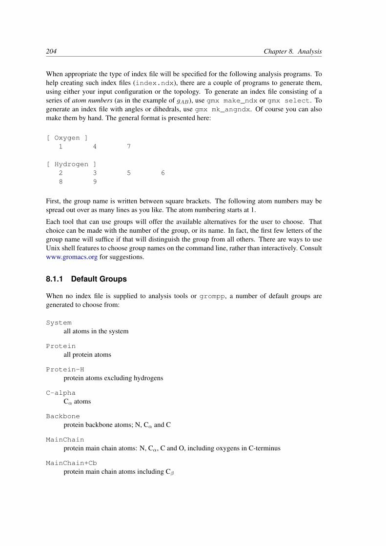
204 Chapter 8. Analysis
When appropriate the type of index file will be specified for the following analysis programs. Tohelp creating such index files (index.ndx), there are a couple of programs to generate them,using either your input configuration or the topology. To generate an index file consisting of aseries of atom numbers (as in the example of gAB), use gmx make_ndx or gmx select. Togenerate an index file with angles or dihedrals, use gmx mk_angndx. Of course you can alsomake them by hand. The general format is presented here:
[ Oxygen ]1 4 7
[ Hydrogen ]2 3 5 68 9
First, the group name is written between square brackets. The following atom numbers may bespread out over as many lines as you like. The atom numbering starts at 1.
Each tool that can use groups will offer the available alternatives for the user to choose. Thatchoice can be made with the number of the group, or its name. In fact, the first few letters of thegroup name will suffice if that will distinguish the group from all others. There are ways to useUnix shell features to choose group names on the command line, rather than interactively. Consultwww.gromacs.org for suggestions.
8.1.1 Default Groups
When no index file is supplied to analysis tools or grompp, a number of default groups aregenerated to choose from:
Systemall atoms in the system
Proteinall protein atoms
Protein-Hprotein atoms excluding hydrogens
C-alphaCα atoms
Backboneprotein backbone atoms; N, Cα and C
MainChainprotein main chain atoms: N, Cα, C and O, including oxygens in C-terminus
MainChain+Cbprotein main chain atoms including Cβ

8.1. Using Groups 205
MainChain+Hprotein main chain atoms including backbone amide hydrogens and hydrogens on the N-terminus
SideChainprotein side chain atoms; that is all atoms except N, Cα, C, O, backbone amide hydrogens,oxygens in C-terminus and hydrogens on the N-terminus
SideChain-Hprotein side chain atoms excluding all hydrogens
Prot-Massesprotein atoms excluding dummy masses (as used in virtual site constructions of NH3 groupsand tryptophan side-chains), see also sec. 5.2.2; this group is only included when it differsfrom the “Protein” group
Non-Proteinall non-protein atoms
DNAall DNA atoms
RNAall RNA atoms
Waterwater molecules (names like SOL, WAT, HOH, etc.) See residuetypes.dat for a fulllisting
non-Wateranything not covered by the Water group
Ionany name matching an Ion entry in residuetypes.dat
Water_and_Ionscombination of the Water and Ions groups
molecule_namefor all residues/molecules which are not recognized as protein, DNA, or RNA; one groupper residue/molecule name is generated
Otherall atoms which are neither protein, DNA, nor RNA.
Empty groups will not be generated. Most of the groups only contain protein atoms. An atom isconsidered a protein atom if its residue name is listed in the residuetypes.dat file and islisted as a “Protein” entry. The process for determinding DNA, RNA, etc. is analogous. If youneed to modify these classifications, then you can copy the file from the library directory into yourworking directory and edit the local copy.

206 Chapter 8. Analysis
8.1.2 Selections
gmx selectCurrently, a few analysis tools support an extended concept of (dynamic) selections. There arethree main differences to traditional index groups:
• The selections are specified as text instead of reading fixed atom indices from a file, usinga syntax similar to VMD. The text can be entered interactively, provided on the commandline, or from a file.
• The selections are not restricted to atoms, but can also specify that the analysis is to beperformed on, e.g., center-of-mass positions of a group of atoms. Some tools may notsupport selections that do not evaluate to single atoms, e.g., if they require information thatis available only for single atoms, like atom names or types.
• The selections can be dynamic, i.e., evaluate to different atoms for different trajectoryframes. This allows analyzing only a subset of the system that satisfies some geometriccriteria.
As an example of a simple selection, resname ABC and within 2 of resname DEFselects all atoms in residues named ABC that are within 2 nm of any atom in a residue namedDEF.
Tools that accept selections can also use traditional index files similarly to older tools: it is possibleto give an .ndx file to the tool, and directly select a group from the index file as a selection, eitherby group number or by group name. The index groups can also be used as a part of a morecomplicated selection.
To get started, you can run gmx select with a single structure, and use the interactive promptto try out different selections. The tool provides, among others, output options -on and -ofpdbto write out the selected atoms to an index file and to a .pdb file, respectively. This does not allowtesting selections that evaluate to center-of-mass positions, but other selections can be tested andthe result examined.
The detailed syntax and the individual keywords that can be used in selections can be accessed bytyping help in the interactive prompt of any selection-enabled tool, as well as with gmx helpselections. The help is divided into subtopics that can be accessed with, e.g., help syntax/ gmx help selections syntax. Some individual selection keywords have extended helpas well, which can be accessed with, e.g., help keywords within.
The interactive prompt does not currently provide much editing capabilities. If you need them,you can run the program under rlwrap.
For tools that do not yet support the selection syntax, you can use gmx select -on to generatestatic index groups to pass to the tool. However, this only allows for a small subset (only the firstbullet from the above list) of the flexibility that fully selection-aware tools offer.
It is also possible to write your own analysis tools to take advantage of the flexibility of theseselections: see the template.cpp file in the share/gromacs/template directory of yourinstallation for an example.

8.2. Looking at your trajectory 207
Figure 8.1: The window of gmx view showing a box of water.
8.2 Looking at your trajectory
gmx viewBefore analyzing your trajectory it is often informative to look at your trajectory first. GROMACScomes with a simple trajectory viewer gmx view; the advantage with this one is that it does notrequire OpenGL, which usually isn’t present on e.g. supercomputers. It is also possible to generatea hard-copy in Encapsulated Postscript format (see Fig. 8.1). If you want a faster and more fancyviewer there are several programs that can read the GROMACS trajectory formats – have a lookat our homepage (www.gromacs.org) for updated links.
8.3 General properties
gmx energy, gmx trajTo analyze some or all energies and other properties, such as total pressure, pressure tensor,density, box-volume and box-sizes, use the program gmx energy. A choice can be made froma list a set of energies, like potential, kinetic or total energy, or individual contributions, likeLennard-Jones or dihedral energies.
The center-of-mass velocity, defined as
vcom =1
M
N∑i=1
mivi (8.2)
with M =∑Ni=1mi the total mass of the system, can be monitored in time by the program gmx
traj -com -ov. It is however recommended to remove the center-of-mass velocity every step(see chapter 3)!

208 Chapter 8. Analysis
r
r+dr r+dr
rθ+dθ
θ
e
A B
DC
Figure 8.2: Definition of slices in gmx rdf: A. gAB(r). B. gAB(r, θ). The slices are colored gray.C. Normalization 〈ρB〉local. D. Normalization 〈ρB〉local, θ. Normalization volumes are coloredgray.
8.4 Radial distribution functions
gmx rdfThe radial distribution function (RDF) or pair correlation function gAB(r) between particles oftype A and B is defined in the following way:
gAB(r) =〈ρB(r)〉〈ρB〉local
=1
〈ρB〉local1
NA
NA∑i∈A
NB∑j∈B
δ(rij − r)4πr2
(8.3)
with 〈ρB(r)〉 the particle density of type B at a distance r around particles A, and 〈ρB〉local theparticle density of type B averaged over all spheres around particles A with radius rmax (seeFig. 8.2C).
Usually the value of rmax is half of the box length. The averaging is also performed in time. Inpractice the analysis program gmx rdf divides the system into spherical slices (from r to r+dr,see Fig. 8.2A) and makes a histogram in stead of the δ-function. An example of the RDF ofoxygen-oxygen in SPC water [85] is given in Fig. 8.3.
With gmx rdf it is also possible to calculate an angle dependent rdf gAB(r, θ), where the angleθ is defined with respect to a certain laboratory axis e, see Fig. 8.2B.
gAB(r, θ) =1
〈ρB〉local, θ1
NA
NA∑i∈A
NB∑j∈B
δ(rij − r)δ(θij − θ)2πr2sin(θ)
(8.4)
cos(θij) =rij · e‖rij‖ ‖e‖
(8.5)

8.4. Radial distribution functions 209
0 0.2 0.4 0.6 0.8
r (nm)
0
0.5
1
1.5
2
2.5
3
g(r
)
Figure 8.3: gOO(r) for Oxygen-Oxygen of SPC-water.

210 Chapter 8. Analysis
This gAB(r, θ) is useful for analyzing anisotropic systems. Note that in this case the normalization〈ρB〉local, θ is the average density in all angle slices from θ to θ+dθ up to rmax, so angle dependent,see Fig. 8.2D.
8.5 Correlation functions
8.5.1 Theory of correlation functions
The theory of correlation functions is well established [113]. We describe here the implemen-tation of the various correlation function flavors in the GROMACS code. The definition of theautocorrelation function (ACF) Cf (t) for a property f(t) is:
Cf (t) = 〈f(ξ)f(ξ + t)〉ξ (8.6)
where the notation on the right hand side indicates averaging over ξ, i.e. over time origins. It isalso possible to compute cross-correlation function from two properties f(t) and g(t):
Cfg(t) = 〈f(ξ)g(ξ + t)〉ξ (8.7)
however, in GROMACS there is no standard mechanism to do this (note: you can use the xmgrprogram to compute cross correlations). The integral of the correlation function over time is thecorrelation time τf :
τf =
∫ ∞0
Cf (t)dt (8.8)
In practice, correlation functions are calculated based on data points with discrete time intervals∆t, so that the ACF from an MD simulation is:
Cf (j∆t) =1
N − j
N−1−j∑i=0
f(i∆t)f((i+ j)∆t) (8.9)
whereN is the number of available time frames for the calculation. The resulting ACF is obviouslyonly available at time points with the same interval ∆t. Since, for many applications, it is necessaryto know the short time behavior of the ACF (e.g. the first 10 ps) this often means that we have tosave the data with intervals much shorter than the time scale of interest. Another implication ofeqn. 8.9 is that in principle we can not compute all points of the ACF with the same accuracy, sincewe have N − 1 data points for Cf (∆t) but only 1 for Cf ((N − 1)∆t). However, if we decide tocompute only an ACF of length M∆t, where M ≤ N/2 we can compute all points with the samestatistical accuracy:
Cf (j∆t) =1
M
N−1−M∑i=0
f(i∆t)f((i+ j)∆t) (8.10)
Here of course j < M . M is sometimes referred to as the time lag of the correlation function.When we decide to do this, we intentionally do not use all the available points for very short timeintervals (j << M ), but it makes it easier to interpret the results. Another aspect that may not beneglected when computing ACFs from simulation is that usually the time origins ξ (eqn. 8.6) arenot statistically independent, which may introduce a bias in the results. This can be tested using a
8.5. Correlation functions 211
block-averaging procedure, where only time origins with a spacing at least the length of the timelag are included, e.g. using k time origins with spacing of M∆t (where kM ≤ N ):
Cf (j∆t) =1
k
k−1∑i=0
f(iM∆t)f((iM + j)∆t) (8.11)
However, one needs very long simulations to get good accuracy this way, because there are manyfewer points that contribute to the ACF.
8.5.2 Using FFT for computation of the ACF
The computational cost for calculating an ACF according to eqn. 8.9 is proportional to N2, whichis considerable. However, this can be improved by using fast Fourier transforms to do the convo-lution [113].
8.5.3 Special forms of the ACF
There are some important varieties on the ACF, e.g. the ACF of a vector p:
Cp(t) =
∫ ∞0
Pn(cos 6 (p(ξ),p(ξ + t)) dξ (8.12)
where Pn(x) is the nth order Legendre polynomial 1. Such correlation times can actually be ob-tained experimentally using e.g. NMR or other relaxation experiments. GROMACS can computecorrelations using the 1st and 2nd order Legendre polynomial (eqn. 8.12). This can also be usedfor rotational autocorrelation (gmx rotacf) and dipole autocorrelation (gmx dipoles).
In order to study torsion angle dynamics, we define a dihedral autocorrelation function as [164]:
C(t) = 〈cos(θ(τ)− θ(τ + t))〉τ (8.13)
Note that this is not a product of two functions as is generally used for correlation functions, butit may be rewritten as the sum of two products:
C(t) = 〈cos(θ(τ)) cos(θ(τ + t)) + sin(θ(τ)) sin(θ(τ + t))〉τ (8.14)
8.5.4 Some Applications
The program gmx velacc calculates the velocity autocorrelation function.
Cv(τ) = 〈vi(τ) · vi(0)〉i∈A (8.15)
The self diffusion coefficient can be calculated using the Green-Kubo relation [113]:
DA =1
3
∫ ∞0〈vi(t) · vi(0)〉i∈A dt (8.16)
1P0(x) = 1, P1(x) = x, P2(x) = (3x2 − 1)/2

212 Chapter 8. Analysis
which is just the integral of the velocity autocorrelation function. There is a widely-held beliefthat the velocity ACF converges faster than the mean square displacement (sec. 8.7), which canalso be used for the computation of diffusion constants. However, Allen & Tildesley [113] warnus that the long-time contribution to the velocity ACF can not be ignored, so care must be taken.
Another important quantity is the dipole correlation time. The dipole correlation function forparticles of type A is calculated as follows by gmx dipoles:
Cµ(τ) = 〈µi(τ) · µi(0)〉i∈A (8.17)
with µi =∑j∈i rjqj . The dipole correlation time can be computed using eqn. 8.8. For some
applications see [165].
The viscosity of a liquid can be related to the correlation time of the Pressure tensor P [166, 167].gmx energy can compute the viscosity, but this is not very accurate [154], and actually thevalues do not converge.
8.6 Curve fitting in GROMACS
8.6.1 Sum of exponential functions
Sometimes it is useful to fit a curve to an analytical function, for example in the case of autocor-relation functions with noisy tails. GROMACS is not a general purpose curve-fitting tool howeverand therefore GROMACS only supports a limited number of functions. Table 8.1 lists the avail-able options with the corresponding command-line options. The underlying routines for fitting usethe Levenberg-Marquardt algorithm as implemented in the lmfit package [168] (a bare-bonesversion of which is included in GROMACS in which an option for error-weighted fitting wasimplemented).
Table 8.1: Overview of fitting functions supported in (most) analysis tools that compute autocor-relation functions. The “Note” column describes properties of the output parameters.
Command Functional form f(t) Noteline optionexp e−t/a0
aexp a1e−t/a0
exp_exp a1e−t/a0 + (1− a1)e−t/a2 a2 ≥ a0 ≥ 0
exp5 a1e−t/a0 + a3e
−t/a2 + a4 a2 ≥ a0 ≥ 0
exp7 a1e−t/a0 + a3e
−t/a2 + a5e−t/a4 + a6 a4 ≥ a2 ≥ a0 ≥ 0
exp9 a1e−t/a0 + a3e
−t/a2 + a5e−t/a4 + a7e
−t/a6 + a8 a6 ≥ a4 ≥ a2 ≥ a0 ≥ 0
8.6.2 Error estimation
Under the hood GROMACS implements some more fitting functions, namely a function to esti-mate the error in time-correlated data due to Hess [154]:
ε2(t) = ατ1
(1 +
τ1
t
(e−t/τ1 − 1
))+ (1− α)τ2
(1 +
τ2
t
(e−t/τ2 − 1
))(8.18)
8.6. Curve fitting in GROMACS 213
where τ1 and τ2 are time constants (with τ2 ≥ τ1) and α usually is close to 1 (in the fittingprocedure it is enforced that 0 ≤ α ≤ 1). This is used in gmx analyze for error estimationusing
limt→∞
ε(t) = σ
√2(ατ1 + (1− α)τ2)
T(8.19)
where σ is the standard deviation of the data set and T is the total simulation time [154].
8.6.3 Interphase boundary demarcation
In order to determine the position and width of an interface, Steen-Sæthre et al. fitted a densityprofile to the following function
f(x) =a0 + a1
2− a0 − a1
2erf
(x− a2
a23
)(8.20)
where a0 and a1 are densities of different phases, x is the coordinate normal to the interface, a2 isthe position of the interface and a3 is the width of the interface [169]. This is implemented in gmxdensorder.
8.6.4 Transverse current autocorrelation function
In order to establish the transverse current autocorrelation function (useful for computing viscos-ity [170]) the following function is fitted:
f(x) = e−ν(
cosh(ων) +sinh(ων)
ω
)(8.21)
with ν = x/(2a0) and ω =√
1− a1. This is implemented in gmx tcaf.
8.6.5 Viscosity estimation from pressure autocorrelation function
The viscosity is a notoriously difficult property to extract from simulations [154, 171]. It is inprinciple possible to determine it by integrating the pressure autocorrelation function [166], how-ever this is often hampered by the noisy tail of the ACF. A workaround to this is fitting the ACFto the following function [172]:
f(t)/f(0) = (1− C)cos(ωt)e−(t/τf )βf
+ Ce−(t/τs)βs (8.22)
where ω is the frequency of rapid pressure oscillations (mainly due to bonded forces in molecu-lar simulations), τf and βf are the time constant and exponent of fast relaxation in a stretched-exponential approximation, τs and βs are constants for slow relaxation and C is the pre-factor thatdetermines the weight between fast and slow relaxation. After a fit, the integral of the functionf(t) is used to compute the viscosity:
η =V
kBT
∫ ∞0
f(t)dt (8.23)
This equation has been applied to computing the bulk and shear viscosity using different elementsfrom the pressure tensor [173]. This is implemented in gmx viscosity.

214 Chapter 8. Analysis
0.0 50.0 100.0 150.0Time (ps)
0.0
1000.0
2000.0
3000.0
4000.0
MS
D (
10-5 c
m2 s
-1)
Mean Square DisplacementD = 3.5027 (10
-5 cm
2 s
-1)
Figure 8.4: Mean Square Displacement of SPC-water.
8.7 Mean Square Displacement
gmx msdTo determine the self diffusion coefficient DA of particles of type A, one can use the Einsteinrelation [113]:
limt→∞〈‖ri(t)− ri(0)‖2〉i∈A = 6DAt (8.24)
This mean square displacement and DA are calculated by the program gmx msd. Normallyan index file containing atom numbers is used and the MSD is averaged over these atoms. Formolecules consisting of more than one atom, ri can be taken as the center of mass positions ofthe molecules. In that case, you should use an index file with molecule numbers. The results willbe nearly identical to averaging over atoms, however. The gmx msd program can also be usedfor calculating diffusion in one or two dimensions. This is useful for studying lateral diffusion oninterfaces.
An example of the mean square displacement of SPC water is given in Fig. 8.4.
8.8 Bonds/distances, angles and dihedrals
gmx distance, gmx angle, gmx gangleTo monitor specific bonds in your modules, or more generally distances between points, the pro-gram gmx distance can calculate distances as a function of time, as well as the distribution ofthe distance. With a traditional index file, the groups should consist of pairs of atom numbers, forexample:
[ bonds_1 ]1 23 4
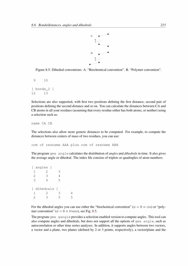
8.8. Bonds/distances, angles and dihedrals 215
φ = 0φ = 0
AB
Figure 8.5: Dihedral conventions: A. “Biochemical convention”. B. “Polymer convention”.
9 10
[ bonds_2 ]12 13
Selections are also supported, with first two positions defining the first distance, second pair ofpositions defining the second distance and so on. You can calculate the distances between CA andCB atoms in all your residues (assuming that every residue either has both atoms, or neither) usinga selection such as:
name CA CB
The selections also allow more generic distances to be computed. For example, to compute thedistances between centers of mass of two residues, you can use:
com of resname AAA plus com of resname BBB
The program gmx angle calculates the distribution of angles and dihedrals in time. It also givesthe average angle or dihedral. The index file consists of triplets or quadruples of atom numbers:
[ angles ]1 2 32 3 43 4 5
[ dihedrals ]1 2 3 42 3 5 5
For the dihedral angles you can use either the “biochemical convention” (φ = 0 ≡ cis) or “poly-mer convention” (φ = 0 ≡ trans), see Fig. 8.5.
The program gmx gangle provides a selection-enabled version to compute angles. This tool canalso compute angles and dihedrals, but does not support all the options of gmx angle, such asautocorrelation or other time series analyses. In addition, it supports angles between two vectors,a vector and a plane, two planes (defined by 2 or 3 points, respectively), a vector/plane and the

216 Chapter 8. Analysis
A B C
z
D
Figure 8.6: Angle options of gmx gangle: A. Angle between two vectors. B. Angle betweentwo planes. C. Angle between a vector and the z axis. D. Angle between a vector and the normal ofa sphere. Also other combinations are supported: planes and vectors can be used interchangeably.
z axis, or a vector/plane and the normal of a sphere (determined by a single position). Also theangle between a vector/plane compared to its position in the first frame is supported. For planes,gmx gangle uses the normal vector perpendicular to the plane. See Fig. 8.6A, B, C) for thedefinitions.
8.9 Radius of gyration and distances
gmx gyrate, gmx distance, gmx mindist, gmx mdmat, gmx pairdist, gmxxpm2psTo have a rough measure for the compactness of a structure, you can calculate the radius of gyra-tion with the program gmx gyrate as follows:
Rg =
(∑i ‖ri‖2mi∑
imi
) 12
(8.25)
where mi is the mass of atom i and ri the position of atom i with respect to the center of mass ofthe molecule. It is especially useful to characterize polymer solutions and proteins. The programwill also provide the radius of gyration around the coordinate axis (or, optionally, principal axes)by only summing the radii components orthogonal to each axis, for instance
Rg,x =
∑i
(r2i,y + r2
i,z
)mi∑
imi
12
(8.26)
Sometimes it is interesting to plot the distance between two atoms, or the minimum distance be-tween two groups of atoms (e.g.: protein side-chains in a salt bridge). To calculate these distancesbetween certain groups there are several possibilities:
• The distance between the geometrical centers of two groups can be calculated with the programgmx distance, as explained in sec. 8.8.
• The minimum distance between two groups of atoms during time can be calculated with theprogram gmx mindist. It also calculates the number of contacts between these groupswithin a certain radius rmax.

8.10. Root mean square deviations in structure 217
21 30 40 50 60 70 80 90
21
30
40
50
60
70
80
90
t=0
ps
Residue Number
0 Distance (nm) 1.2
Figure 8.7: A minimum distance matrix for a peptide [174].
• gmx pairdist is a selection-enabled version of gmx mindist.
• To monitor the minimum distances between amino acid residues within a (protein) molecule,you can use the program gmx mdmat. This minimum distance between two residues Ai
and Aj is defined as the smallest distance between any pair of atoms (i ∈ Ai, j ∈ Aj). Theoutput is a symmetrical matrix of smallest distances between all residues. To visualize thismatrix, you can use a program such as xv. If you want to view the axes and legend or ifyou want to print the matrix, you can convert it with xpm2ps into a Postscript picture, seeFig. 8.7.
Plotting these matrices for different time-frames, one can analyze changes in the structure,and e.g. forming of salt bridges.
8.10 Root mean square deviations in structure
gmx rms, gmx rmsdistThe root mean square deviation (RMSD) of certain atoms in a molecule with respect to a refer-ence structure can be calculated with the program gmx rms by least-square fitting the structureto the reference structure (t2 = 0) and subsequently calculating the RMSD (eqn. 8.27).
RMSD(t1, t2) =
[1
M
N∑i=1
mi‖ri(t1)− ri(t2)‖2] 1
2
(8.27)
where M =∑Ni=1mi and ri(t) is the position of atom i at time t. Note that fitting does not
have to use the same atoms as the calculation of the RMSD; e.g. a protein is usually fitted on

218 Chapter 8. Analysis
the backbone atoms (N,Cα,C), but the RMSD can be computed of the backbone or of the wholeprotein.
Instead of comparing the structures to the initial structure at time t = 0 (so for example a crystalstructure), one can also calculate eqn. 8.27 with a structure at time t2 = t1 − τ . This gives someinsight in the mobility as a function of τ . A matrix can also be made with theRMSD as a functionof t1 and t2, which gives a nice graphical interpretation of a trajectory. If there are transitions in atrajectory, they will clearly show up in such a matrix.
Alternatively theRMSD can be computed using a fit-free method with the program gmx rmsdist:
RMSD(t) =
1
N2
N∑i=1
N∑j=1
‖rij(t)− rij(0)‖2 1
2
(8.28)
where the distance rij between atoms at time t is compared with the distance between the sameatoms at time 0.
8.11 Covariance analysis
Covariance analysis, also called principal component analysis or essential dynamics [175], canfind correlated motions. It uses the covariance matrix C of the atomic coordinates:
Cij =
⟨M
12ii (xi − 〈xi〉)M
12jj(xj − 〈xj〉)
⟩(8.29)
where M is a diagonal matrix containing the masses of the atoms (mass-weighted analysis) orthe unit matrix (non-mass weighted analysis). C is a symmetric 3N × 3N matrix, which can bediagonalized with an orthonormal transformation matrix R:
RTCR = diag(λ1, λ2, . . . , λ3N ) where λ1 ≥ λ2 ≥ . . . ≥ λ3N (8.30)
The columns of R are the eigenvectors, also called principal or essential modes. R defines atransformation to a new coordinate system. The trajectory can be projected on the principal modesto give the principal components pi(t):
p(t) = RTM12 (x(t)− 〈x〉) (8.31)
The eigenvalue λi is the mean square fluctuation of principal component i. The first few principalmodes often describe collective, global motions in the system. The trajectory can be filtered alongone (or more) principal modes. For one principal mode i this goes as follows:
xf (t) = 〈x〉+M−12R∗i pi(t) (8.32)
When the analysis is performed on a macromolecule, one often wants to remove the overall rota-tion and translation to look at the internal motion only. This can be achieved by least square fittingto a reference structure. Care has to be taken that the reference structure is representative for theensemble, since the choice of reference structure influences the covariance matrix.

8.11. Covariance analysis 219
One should always check if the principal modes are well defined. If the first principal componentresembles a half cosine and the second resembles a full cosine, you might be filtering noise (seebelow). A good way to check the relevance of the first few principal modes is to calculate theoverlap of the sampling between the first and second half of the simulation. Note that this canonly be done when the same reference structure is used for the two halves.
A good measure for the overlap has been defined in [176]. The elements of the covariance matrixare proportional to the square of the displacement, so we need to take the square root of the matrixto examine the extent of sampling. The square root can be calculated from the eigenvalues λi andthe eigenvectors, which are the columns of the rotation matrixR. For a symmetric and diagonally-dominant matrix A of size 3N × 3N the square root can be calculated as:
A12 = R diag(λ
121 , λ
122 , . . . , λ
123N )RT (8.33)
It can be verified easily that the product of this matrix with itself gives A. Now we can define adifference d between covariance matrices A and B as follows:
d(A,B) =
√tr((A
12 −B
12
)2)
(8.34)
=
√tr(A+B − 2A
12B
12
)(8.35)
=
N∑i=1
(λAi + λBi
)− 2
N∑i=1
N∑j=1
√λAi λ
Bj
(RAi ·RBj
)2
12
(8.36)
where tr is the trace of a matrix. We can now define the overlap s as:
s(A,B) = 1− d(A,B)√trA+ trB
(8.37)
The overlap is 1 if and only if matrices A and B are identical. It is 0 when the sampled subspacesare completely orthogonal.
A commonly-used measure is the subspace overlap of the first few eigenvectors of covariancematrices. The overlap of the subspace spanned by m orthonormal vectors w1, . . . ,wm with areference subspace spanned by n orthonormal vectors v1, . . . ,vn can be quantified as follows:
overlap(v,w) =1
n
n∑i=1
m∑j=1
(vi ·wj)2 (8.38)
The overlap will increase with increasing m and will be 1 when set v is a subspace of set w.The disadvantage of this method is that it does not take the eigenvalues into account. All eigen-vectors are weighted equally, and when degenerate subspaces are present (equal eigenvalues), thecalculated overlap will be too low.
Another useful check is the cosine content. It has been proven that the the principal componentsof random diffusion are cosines with the number of periods equal to half the principal componentindex [177, 176]. The eigenvalues are proportional to the index to the power −2. The cosinecontent is defined as:
2
T
(∫ T
0cos
(iπt
T
)pi(t)dt
)2(∫ T
0p2i (t)dt
)−1
(8.39)

220 Chapter 8. Analysis
D
H
α
A
r
Figure 8.8: Geometrical Hydrogen bond criterion.
When the cosine content of the first few principal components is close to 1, the largest fluctuationsare not connected with the potential, but with random diffusion.
The covariance matrix is built and diagonalized by gmx covar. The principal components andoverlap (and many more things) can be plotted and analyzed with gmx anaeig. The cosinecontent can be calculated with gmx analyze.
8.12 Dihedral principal component analysis
gmx angle, gmx covar, gmx anaeigPrincipal component analysis can be performed in dihedral space [178] using GROMACS. Youstart by defining the dihedral angles of interest in an index file, either using gmx mk_angndxor otherwise. Then you use the gmx angle program with the -or flag to produce a new .trrfile containing the cosine and sine of each dihedral angle in two coordinates, respectively. Thatis, in the .trr file you will have a series of numbers corresponding to: cos(φ1), sin(φ1), cos(φ2),sin(φ2), ..., cos(φn), sin(φn), and the array is padded with zeros, if necessary. Then you can usethis .trr file as input for the gmx covar program and perform principal component analysisas usual. For this to work you will need to generate a reference file (.tpr, .gro, .pdb etc.)containing the same number of “atoms” as the new .trr file, that is for n dihedrals you need2n/3 atoms (rounded up if not an integer number). You should use the -nofit option for gmxcovar since the coordinates in the dummy reference file do not correspond in any way to theinformation in the .trr file. Analysis of the results is done using gmx anaeig.
8.13 Hydrogen bonds
gmx hbondThe program gmx hbond analyzes the hydrogen bonds (H-bonds) between all possible donorsD and acceptors A. To determine if an H-bond exists, a geometrical criterion is used, see alsoFig. 8.8:
r ≤ rHB = 0.35 nmα ≤ αHB = 30o
(8.40)
The value of rHB = 0.35 nm corresponds to the first minimum of the RDF of SPC water (see alsoFig. 8.3).
The program gmx hbond analyzes all hydrogen bonds existing between two groups of atoms(which must be either identical or non-overlapping) or in specified donor-hydrogen-acceptor triplets,

8.13. Hydrogen bonds 221
O
DA
H
H
H
(1)(2)
(2)Figure 8.9: Insertion of water into an H-bond. (1) Normal H-bond between two residues. (2)H-bonding bridge via a water molecule.
in the following ways:
• Donor-Acceptor distance (r) distribution of all H-bonds
• Hydrogen-Donor-Acceptor angle (α) distribution of all H-bonds
• The total number of H-bonds in each time frame
• The number of H-bonds in time between residues, divided into groups n-n+i where n andn+i stand for residue numbers and i goes from 0 to 6. The group for i = 6 also includesall H-bonds for i > 6. These groups include the n-n+3, n-n+4 and n-n+5 H-bonds, whichprovide a measure for the formation of α-helices or β-turns or strands.
• The lifetime of the H-bonds is calculated from the average over all autocorrelation functionsof the existence functions (either 0 or 1) of all H-bonds:
C(τ) = 〈si(t) si(t+ τ)〉 (8.41)
with si(t) = 0, 1 for H-bond i at time t. The integral of C(τ) gives a rough estimate ofthe average H-bond lifetime τHB:
τHB =
∫ ∞0
C(τ)dτ (8.42)
Both the integral and the complete autocorrelation functionC(τ) will be output, so that moresophisticated analysis (e.g. using multi-exponential fits) can be used to get better estimatesfor τHB . A more complete analysis is given in ref. [179]; one of the more fancy option isthe Luzar and Chandler analysis of hydrogen bond kinetics [180, 181].
• An H-bond existence map can be generated of dimensions # H-bonds×# frames. The order-ing is identical to the index file (see below), but reversed, meaning that the last triplet in theindex file corresponds to the first row of the existence map.
• Index groups are output containing the analyzed groups, all donor-hydrogen atom pairsand acceptor atoms in these groups, donor-hydrogen-acceptor triplets involved in hydrogenbonds between the analyzed groups and all solvent atoms involved in insertion.

222 Chapter 8. Analysis
8.14 Protein-related items
gmx do_dssp, gmx rama, gmx wheelTo analyze structural changes of a protein, you can calculate the radius of gyration or the minimumresidue distances over time (see sec. 8.9), or calculate the RMSD (sec. 8.10).
You can also look at the changing of secondary structure elements during your run. For this,you can use the program gmx do_dssp, which is an interface for the commercial programDSSP [182]. For further information, see the DSSP manual. A typical output plot of gmx do_-dssp is given in Fig. 8.10.
One other important analysis of proteins is the so-called Ramachandran plot. This is the projectionof the structure on the two dihedral angles φ and ψ of the protein backbone, see Fig. 8.11.
To evaluate this Ramachandran plot you can use the program gmx rama. A typical output isgiven in Fig. 8.12.
When studying α-helices it is useful to have a helical wheel projection of your peptide, to seewhether a peptide is amphipathic. This can be done using the gmx wheel program. Two exam-ples are plotted in Fig. 8.13.
8.15 Interface-related items
gmx order, gmx density, gmx potential, gmx trajWhen simulating molecules with long carbon tails, it can be interesting to calculate their averageorientation. There are several flavors of order parameters, most of which are related. The programgmx order can calculate order parameters using the equation:
Sz =3
2〈cos2 θz〉 −
1
2(8.43)
where θz is the angle between the z-axis of the simulation box and the molecular axis underconsideration. The latter is defined as the vector from Cn−1 to Cn+1. The parameters Sx and Sy aredefined in the same way. The brackets imply averaging over time and molecules. Order parameterscan vary between 1 (full order along the interface normal) and −1/2 (full order perpendicular tothe normal), with a value of zero in the case of isotropic orientation.
The program can do two things for you. It can calculate the order parameter for each CH2 segmentseparately, for any of three axes, or it can divide the box in slices and calculate the average valueof the order parameter per segment in one slice. The first method gives an idea of the ordering ofa molecule from head to tail, the second method gives an idea of the ordering as function of thebox length.
The electrostatic potential (ψ) across the interface can be computed from a trajectory by evaluatingthe double integral of the charge density (ρ(z)):
ψ(z)− ψ(−∞) = −∫ z
−∞dz′
∫ z′
−∞ρ(z′′)dz′′/ε0 (8.44)
where the position z = −∞ is far enough in the bulk phase such that the field is zero. With thismethod, it is possible to “split” the total potential into separate contributions from lipid and water

8.15. Interface-related items 223
0 100 200 300 400 500 600 700 800 900 1000
1
5
10
15
Res
idue
Time (ps)Coil Bend Turn A-Helix B-Bridge
Figure 8.10: Analysis of the secondary structure elements of a peptide in time.
C
O
N
CH
R
C
Oα
N
H
H
ψφ
Figure 8.11: Definition of the dihedral angles φ and ψ of the protein backbone.
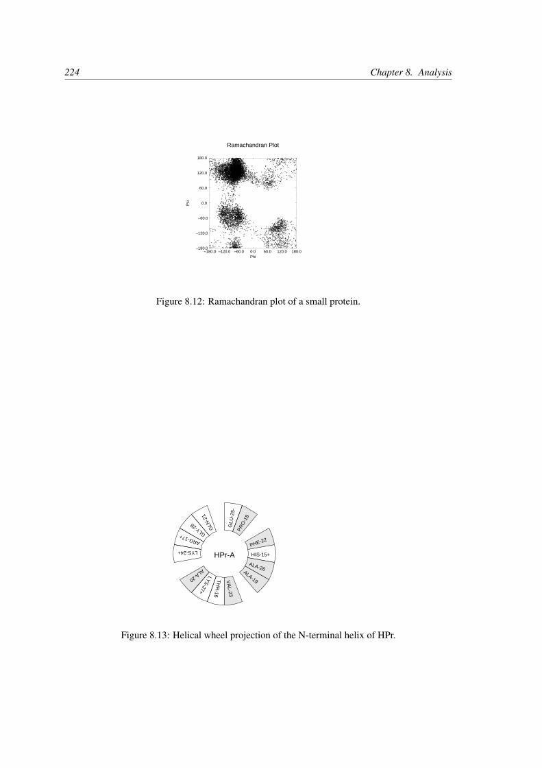
224 Chapter 8. Analysis
–180.0 –120.0 –60.0 0.0 60.0 120.0 180.0Phi
–180.0
–120.0
–60.0
0.0
60.0
120.0
180.0
Psi
Ramachandran Plot
Figure 8.12: Ramachandran plot of a small protein.
HPr-A HIS-15+
TH
R-16
ARG-17+
PRO
-18
ALA-19
ALA-20
GLN
-21
PHE-22
VA
L-23
LYS-24+
GLU
-25-
ALA-26
LYS-27+
GLY-28
Figure 8.13: Helical wheel projection of the N-terminal helix of HPr.

8.15. Interface-related items 225
molecules. The program gmx potential divides the box in slices and sums all charges of theatoms in each slice. It then integrates this charge density to give the electric field, which is in turnintegrated to give the potential. Charge density, electric field, and potential are written to xvgrinput files.
The program gmx traj is a very simple analysis program. All it does is print the coordinates,velocities, or forces of selected atoms. It can also calculate the center of mass of one or moremolecules and print the coordinates of the center of mass to three files. By itself, this is probablynot a very useful analysis, but having the coordinates of selected molecules or atoms can be veryhandy for further analysis, not only in interfacial systems.
The program gmx density calculates the mass density of groups and gives a plot of the densityagainst a box axis. This is useful for looking at the distribution of groups or atoms across theinterface.

226 Chapter 8. Analysis

Appendix A
Some implementation details
In this chapter we will present some implementation details. This is far from complete, but wedeemed it necessary to clarify some things that would otherwise be hard to understand.
A.1 Single Sum Virial in GROMACS
The virial Ξ can be written in full tensor form as:
Ξ = −1
2
N∑i<j
rij ⊗ F ij (A.1)
where ⊗ denotes the direct product of two vectors.1 When this is computed in the inner loop ofan MD program 9 multiplications and 9 additions are needed.2
Here it is shown how it is possible to extract the virial calculation from the inner loop [183].
A.1.1 Virial
In a system with periodic boundary conditions, the periodicity must be taken into account for thevirial:
Ξ = −1
2
N∑i<j
rnij ⊗ F ij (A.2)
where rnij denotes the distance vector of the nearest image of atom i from atom j. In this definitionwe add a shift vector δi to the position vector ri of atom i. The difference vector rnij is thus equalto:
rnij = ri + δi − rj (A.3)
or in shorthand:rnij = rni − rj (A.4)
1(u⊗ v)αβ = uαvβ2The calculation of Lennard-Jones and Coulomb forces is about 50 floating point operations.

228 Appendix A. Some implementation details
In a triclinic system, there are 27 possible images of i; when a truncated octahedron is used, thereare 15 possible images.
A.1.2 Virial from non-bonded forces
Here the derivation for the single sum virial in the non-bonded force routine is given. There are acouple of considerations that are special to GROMACS that we take into account:
• When calculating short-range interactions, we apply the minimum image convention andonly consider the closest image of each neighbor - and in particular we never allow inter-actions between a particle and any of its periodic images. For all the equations below, thismeans i 6= j.
• In general, either the i or j particle might be shifted to a neighbor cell to get the closestinteraction (shift δij). However, with minimum image convention there can be at most 27different shifts for particles in the central cell, and for typical (very short-ranged) biomolec-ular interactions there are typically only a few different shifts involved for each particle, notto mention that each interaction can only be present for one shift.
• For the GROMACS nonbonded interactions we use this to split the neighborlist of each iparticle into multiple separate lists, where each list has a constant shift δi for the i partlcle.We can represent this as a sum over shifts (for which we use index s), with the constraintthat each particle interaction can only contribute to one of the terms in this sum, and theshift is no longer dependent on the j particles. For any sum that does not contain complexdependence on s, this means the sum trivially reduces to just the sum over i and/or j.
• To simplify some of the sums, we replace sums over j < i with double sums over allparticles (remember, i 6= j) and divide by 2.
Starting from the above definition of the virial, we then get
Ξ = −1
2
N∑i<j
rnij ⊗ Fij
= −1
2
N∑i<j
(ri + δij − rj)⊗ Fij
= −1
4
N∑i=1
N∑j=1
(ri + δij − rj)⊗ Fij
= −1
4
N∑i=1
∑s
N∑j=1
(ri + δi,s − rj)⊗ Fij,s
= −1
4
N∑i=
∑s
N∑j=1
((ri + δi,s)⊗ Fij,s − rj ⊗ Fij,s)
= −1
4
N∑i=1
∑s
N∑j=1
(ri + δi,s)⊗ Fij,s +1
4
N∑i=1
∑s
N∑j=1
rj ⊗ Fij,s

A.1. Single Sum Virial in GROMACS 229
= −1
4
N∑i=1
∑s
N∑j=1
(ri + δi,s)⊗ Fij,s +1
4
N∑i=1
N∑j=1
rj ⊗ Fij
= −1
4
∑s
N∑i=1
(ri + δi,s)⊗N∑j=1
Fij,s +1
4
N∑j=1
rj ⊗N∑i=1
Fij
= −1
4
∑s
N∑i=1
(ri + δi,s)⊗N∑j=1
Fij,s −1
4
N∑j=1
rj ⊗N∑i=1
Fji
= −1
4
∑s
N∑i=1
(ri + δi,s)⊗ Fi,s −1
4
N∑j=1
rj ⊗ Fj
= −1
4
N∑i=1
ri ⊗ Fi +N∑j=1
rj ⊗ Fj
− 1
4
∑s
N∑i=1
δi,s ⊗ Fi,s
= −1
2
N∑i=1
ri ⊗ Fi −1
4
∑s
N∑i=1
δi,s ⊗ Fi,s
= −1
2
N∑i=1
ri ⊗ Fi −1
4
∑s
δs ⊗ Fs
= Ξ0 + Ξ1 (A.5)
In the second-last stage, we have used the property that each shift vector itself does not dependon the coordinates of particle i, so it is possible to sum up all forces corresponding to each shiftvector (in the nonbonded kernels), and then just use a sum over the different shift vectors outsidethe kernels. We have also used
F i =N∑j=1
F ij (A.6)
F j =N∑i=1
F ji (A.7)
which is the total force on i with respect to j. Because we use Newton’s Third Law:
F ij = −F ji (A.8)
we must, in the implementation, double the term containing the shift δi. Similarly, in a few placeswe have summed the shift-dependent force over all shifts to come up with the total force perinteraction or particle.
This separates the total virial Ξ into a component Ξ0 that is a single sum over particles, and asecond component Ξ1 that describes the influence of the particle shifts, and that is only a sum overthe different shift vectors.
A.1.3 The intra-molecular shift (mol-shift)
For the bonded forces and SHAKE it is possible to make a mol-shift list, in which the periodicityis stored. We simple have an array mshift in which for each atom an index in the shiftvecarray is stored.

230 Appendix A. Some implementation details
The algorithm to generate such a list can be derived from graph theory, considering each particlein a molecule as a bead in a graph, the bonds as edges.
1 Represent the bonds and atoms as bidirectional graph
2 Make all atoms white
3 Make one of the white atoms black (atom i) and put it in the central box
4 Make all of the neighbors of i that are currently white, gray
5 Pick one of the gray atoms (atom j), give it the correct periodicity with respect to any of itsblack neighbors and make it black
6 Make all of the neighbors of j that are currently white, gray
7 If any gray atom remains, go to [5]
8 If any white atom remains, go to [3]
Using this algorithm we can
• optimize the bonded force calculation as well as SHAKE
• calculate the virial from the bonded forces in the single sum method again
Find a representation of the bonds as a bidirectional graph.
A.1.4 Virial from Covalent Bonds
Since the covalent bond force gives a contribution to the virial, we have:
b = ‖rnij‖ (A.9)
Vb =1
2kb(b− b0)2 (A.10)
F i = −∇Vb (A.11)
= kb(b− b0)rnijb
(A.12)
F j = −F i (A.13)
The virial contribution from the bonds then is:
Ξb = −1
2(rni ⊗ F i + rj ⊗ F j) (A.14)
= −1
2rnij ⊗ F i (A.15)

A.2. Optimizations 231
A.1.5 Virial from SHAKE
An important contribution to the virial comes from shake. Satisfying the constraints a force G thatis exerted on the particles “shaken.” If this force does not come out of the algorithm (as in standardSHAKE) it can be calculated afterward (when using leap-frog) by:
∆ri = ri(t+ ∆t)− [ri(t) + vi(t−∆t
2)∆t+
F i
mi∆t2] (A.16)
Gi =mi∆ri
∆t2(A.17)
This does not help us in the general case. Only when no periodicity is needed (like in rigid water)this can be used, otherwise we must add the virial calculation in the inner loop of SHAKE.
When it is applicable the virial can be calculated in the single sum way:
Ξ = −1
2
Nc∑i
ri ⊗ F i (A.18)
where Nc is the number of constrained atoms.
A.2 Optimizations
Here we describe some of the algorithmic optimizations used in GROMACS, apart from paral-lelism.
A.2.1 Inner Loops for Water
GROMACS uses special inner loops to calculate non-bonded interactions for water molecules withother atoms, and yet another set of loops for interactions between pairs of water molecules. Therehighly optimized loops for two types of water models. For three site models similar to SPC [85],i.e.:
1. There are three atoms in the molecule.
2. The whole molecule is a single charge group.
3. The first atom has Lennard-Jones (sec. 4.1.1) and Coulomb (sec. 4.1.3) interactions.
4. Atoms two and three have only Coulomb interactions, and equal charges.
These loops also works for the SPC/E [184] and TIP3P [133] water models. And for four sitewater models similar to TIP4P [133]:
1. There are four atoms in the molecule.
2. The whole molecule is a single charge group.

232 Appendix A. Some implementation details
3. The first atom has only Lennard-Jones (sec. 4.1.1) interactions.
4. Atoms two and three have only Coulomb (sec. 4.1.3) interactions, and equal charges.
5. Atom four has only Coulomb interactions.
The benefit of these implementations is that there are more floating-point operations in a singleloop, which implies that some compilers can schedule the code better. However, it turns out thateven some of the most advanced compilers have problems with scheduling, implying that manualtweaking is necessary to get optimum performance. This may include common-sub-expressionelimination, or moving code around.
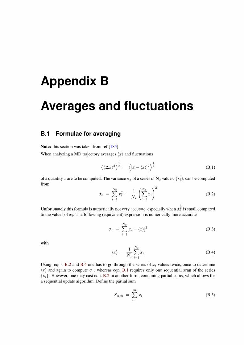
Appendix B
Averages and fluctuations
B.1 Formulae for averaging
Note: this section was taken from ref [185].
When analyzing a MD trajectory averages 〈x〉 and fluctuations
⟨(∆x)2
⟩ 12 =
⟨[x− 〈x〉]2
⟩ 12 (B.1)
of a quantity x are to be computed. The variance σx of a series of Nx values, xi, can be computedfrom
σx =Nx∑i=1
x2i −
1
Nx
(Nx∑i=1
xi
)2
(B.2)
Unfortunately this formula is numerically not very accurate, especially when σ12x is small compared
to the values of xi. The following (equivalent) expression is numerically more accurate
σx =Nx∑i=1
[xi − 〈x〉]2 (B.3)
with
〈x〉 =1
Nx
Nx∑i=1
xi (B.4)
Using eqns. B.2 and B.4 one has to go through the series of xi values twice, once to determine〈x〉 and again to compute σx, whereas eqn. B.1 requires only one sequential scan of the seriesxi. However, one may cast eqn. B.2 in another form, containing partial sums, which allows fora sequential update algorithm. Define the partial sum
Xn,m =m∑i=n
xi (B.5)

234 Appendix B. Averages and fluctuations
and the partial variance
σn,m =m∑i=n
[xi −
Xn,m
m− n+ 1
]2
(B.6)
It can be shown thatXn,m+k = Xn,m +Xm+1,m+k (B.7)
and
σn,m+k = σn,m + σm+1,m+k +
[Xn,m
m− n+ 1− Xn,m+k
m+ k − n+ 1
]2
∗
(m− n+ 1)(m+ k − n+ 1)
k(B.8)
For n = 1 one finds
σ1,m+k = σ1,m + σm+1,m+k +
[X1,m
m− X1,m+k
m+ k
]2 m(m+ k)
k(B.9)
and for n = 1 and k = 1 (eqn. B.8) becomes
σ1,m+1 = σ1,m +
[X1,m
m− X1,m+1
m+ 1
]2
m(m+ 1) (B.10)
= σ1,m +[ X1,m −mxm+1 ]2
m(m+ 1)(B.11)
where we have used the relation
X1,m+1 = X1,m + xm+1 (B.12)
Using formulae (eqn. B.11) and (eqn. B.12) the average
〈x〉 =X1,Nx
Nx(B.13)
and the fluctuation ⟨(∆x)2
⟩ 12 =
[σ1,Nx
Nx
] 12
(B.14)
can be obtained by one sweep through the data.
B.2 Implementation
In GROMACS the instantaneous energiesE(m) are stored in the energy file, along with the valuesof σ1,m andX1,m. Although the steps are counted from 0, for the energy and fluctuations steps arecounted from 1. This means that the equations presented here are the ones that are implemented.We give somewhat lengthy derivations in this section to simplify checking of code and equationslater on.

B.2. Implementation 235
B.2.1 Part of a Simulation
It is not uncommon to perform a simulation where the first part, e.g. 100 ps, is taken as equili-bration. However, the averages and fluctuations as printed in the log file are computed over thewhole simulation. The equilibration time, which is now part of the simulation, may in such a caseinvalidate the averages and fluctuations, because these numbers are now dominated by the initialdrift towards equilibrium.
Using eqns. B.7 and B.8 the average and standard deviation over part of the trajectory can becomputed as:
Xm+1,m+k = X1,m+k −X1,m (B.15)
σm+1,m+k = σ1,m+k − σ1,m −[X1,m
m− X1,m+k
m+ k
]2 m(m+ k)
k(B.16)
or, more generally (with p ≥ 1 and q ≥ p):
Xp,q = X1,q −X1,p−1 (B.17)
σp,q = σ1,q − σ1,p−1 −[X1,p−1
p− 1− X1,q
q
]2 (p− 1)q
q − p+ 1(B.18)
Note that implementation of this is not entirely trivial, since energies are not stored every timestep of the simulation. We therefore have to construct X1,p−1 and σ1,p−1 from the information attime p using eqns. B.11 and B.12:
X1,p−1 = X1,p − xp (B.19)
σ1,p−1 = σ1,p −[ X1,p−1 − (p− 1)xp ]2
(p− 1)p(B.20)
B.2.2 Combining two simulations
Another frequently occurring problem is, that the fluctuations of two simulations must be com-bined. Consider the following example: we have two simulations (A) of n and (B) of m steps, inwhich the second simulation is a continuation of the first. However, the second simulation startsnumbering from 1 instead of from n + 1. For the partial sum this is no problem, we have to addXA
1,n from run A:
XAB1,n+m = XA
1,n +XB1,m (B.21)
When we want to compute the partial variance from the two components we have to make acorrection ∆σ:
σAB1,n+m = σA1,n + σB1,m + ∆σ (B.22)
if we define xABi as the combined and renumbered set of data points we can write:
σAB1,n+m =n+m∑i=1
[xABi −
XAB1,n+m
n+m
]2
(B.23)

236 Appendix B. Averages and fluctuations
and thus
n+m∑i=1
[xABi −
XAB1,n+m
n+m
]2
=n∑i=1
[xAi −
XA1,n
n
]2
+m∑i=1
[xBi −
XB1,m
m
]2
+ ∆σ (B.24)
or
n+m∑i=1
(xABi )2 − 2xABiXAB
1,n+m
n+m+
(XAB
1,n+m
n+m
)2 −
n∑i=1
(xAi )2 − 2xAiXA
1,n
n+
(XA
1,n
n
)2 −
m∑i=1
(xBi )2 − 2xBiXB
1,m
m+
(XB
1,m
m
)2 = ∆σ (B.25)
all the x2i terms drop out, and the terms independent of the summation counter i can be simplified:(
XAB1,n+m
)2
n+m−
(XA
1,n
)2
n−
(XB
1,m
)2
m−
2XAB
1,n+m
n+m
n+m∑i=1
xABi + 2XA
1,n
n
n∑i=1
xAi + 2XB
1,m
m
m∑i=1
xBi = ∆σ (B.26)
we recognize the three partial sums on the second line and use eqn. B.21 to obtain:
∆σ =
(mXA
1,n − nXB1,m
)2
nm(n+m)(B.27)
if we check this by inserting m = 1 we get back eqn. B.11
B.2.3 Summing energy terms
The gmx energy program can also sum energy terms into one, e.g. potential + kinetic = total.For the partial averages this is again easy if we have S energy components s:
XSm,n =
n∑i=m
S∑s=1
xsi =S∑s=1
n∑i=m
xsi =S∑s=1
Xsm,n (B.28)
For the fluctuations it is less trivial again, considering for example that the fluctuation in potentialand kinetic energy should cancel. Nevertheless we can try the same approach as before by writing:
σSm,n =S∑s=1
σsm,n + ∆σ (B.29)
if we fill in eqn. B.6:
n∑i=m
[(S∑s=1
xsi
)−
XSm,n
m− n+ 1
]2
=S∑s=1
n∑i=m
[(xsi )−
Xsm,n
m− n+ 1
]2
+ ∆σ (B.30)

B.2. Implementation 237
which we can expand to:
n∑i=m
S∑s=1
(xsi )2 +
(XSm,n
m− n+ 1
)2
− 2
XSm,n
m− n+ 1
S∑s=1
xsi +S∑s=1
S∑s′=s+1
xsixs′i
−
S∑s=1
n∑i=m
[(xsi )
2 − 2Xsm,n
m− n+ 1xsi +
(Xsm,n
m− n+ 1
)2]
= ∆σ (B.31)
the terms with (xsi )2 cancel, so that we can simplify to:(XSm,n
)2
m− n+ 1− 2
XSm,n
m− n+ 1
n∑i=m
S∑s=1
xsi − 2n∑
i=m
S∑s=1
S∑s′=s+1
xsixs′i −
S∑s=1
n∑i=m
[−2
Xsm,n
m− n+ 1xsi +
(Xsm,n
m− n+ 1
)2]
= ∆σ (B.32)
or
−
(XSm,n
)2
m− n+ 1− 2
n∑i=m
S∑s=1
S∑s′=s+1
xsixs′i +
S∑s=1
(Xsm,n
)2
m− n+ 1= ∆σ (B.33)
If we now expand the first term using eqn. B.28 we obtain:
−
(∑Ss=1X
sm,n
)2
m− n+ 1− 2
n∑i=m
S∑s=1
S∑s′=s+1
xsixs′i +
S∑s=1
(Xsm,n
)2
m− n+ 1= ∆σ (B.34)
which we can reformulate to:
−2
S∑s=1
S∑s′=s+1
Xsm,nX
s′m,n +
n∑i=m
S∑s=1
S∑s′=s+1
xsixs′i
= ∆σ (B.35)
or
−2
S∑s=1
Xsm,n
S∑s′=s+1
Xs′m,n +
S∑s=1
n∑i=m
xsi
S∑s′=s+1
xs′i
= ∆σ (B.36)
which gives
−2S∑s=1
Xsm,n
S∑s′=s+1
n∑i=m
xs′i +
n∑i=m
xsi
S∑s′=s+1
xs′i
= ∆σ (B.37)
Since we need all data points i to evaluate this, in general this is not possible. We can then make anestimate of σSm,n using only the data points that are available using the left hand side of eqn. B.30.While the average can be computed using all time steps in the simulation, the accuracy of thefluctuations is thus limited by the frequency with which energies are saved. Since this can beeasily done with a program such as xmgr this is not built-in in GROMACS.

238 Appendix B. Averages and fluctuations

Bibliography
[1] Bekker, H., Berendsen, H. J. C., Dijkstra, E. J., Achterop, S., van Drunen, R., van derSpoel, D., Sijbers, A., Keegstra, H., Reitsma, B., Renardus, M. K. R. Gromacs: A parallelcomputer for molecular dynamics simulations. In Physics Computing 92 (Singapore, 1993).de Groot, R. A., Nadrchal, J., eds. . World Scientific.
[2] Berendsen, H. J. C., van der Spoel, D., van Drunen, R. GROMACS: A message-passingparallel molecular dynamics implementation. Comp. Phys. Comm. 91:43–56, 1995.
[3] Lindahl, E., Hess, B., van der Spoel, D. GROMACS 3.0: A package for molecular simula-tion and trajectory analysis. J. Mol. Mod. 7:306–317, 2001.
[4] van der Spoel, D., Lindahl, E., Hess, B., Groenhof, G., Mark, A. E., Berendsen, H. J. C.GROMACS: Fast, Flexible and Free. J. Comp. Chem. 26:1701–1718, 2005.
[5] Hess, B., Kutzner, C., van der Spoel, D., Lindahl, E. GROMACS 4: Algorithms for HighlyEfficient, Load-Balanced, and Scalable Molecular Simulation. J. Chem. Theory Comput.4(3):435–447, 2008.
[6] Pronk, S., Páll, S., Schulz, R., Larsson, P., Bjelkmar, P., Apostolov, R., Shirts, M. R., Smith,J. C., Kasson, P. M., van der Spoel, D., Hess, B., Lindahl, E. GROMACS 4.5: a high-throughput and highly parallel open source molecular simulation toolkit. Bioinformatics29(7):845–854, 2013.
[7] Páll, S., Abraham, M. J., Kutzner, C., Hess, B., Lindahl, E. Tackling exascale softwarechallenges in molecular dynamics simulati ons with GROMACS. In: Solving SoftwareChallenges for Exascale. Vol. 8759. Markidis, S., Laure, E. eds. Vol. 8759. . Springer Inter-national Publishing Switzerland London 2015 3–27.
[8] Abraham, M. J., Murtola, T., Schulz, R., Páll, S., Smith, J. C., Hess, B., Lindahl, E. GRO-MACS: High performance molecular simulations through multi-level parallelism from lap-tops to supercomputers. SoftwareX 1–2:19–25, 2015.
[9] van Gunsteren, W. F., Berendsen, H. J. C. Computer simulation of molecular dynamics:Methodology, applications, and perspectives in chemistry. Angew. Chem. Int. Ed. Engl.29:992–1023, 1990.
[10] Fraaije, J. G. E. M. Dynamic density functional theory for microphase separation kineticsof block copolymer melts. J. Chem. Phys. 99:9202–9212, 1993.

240 Bibliography
[11] McQuarrie, D. A. Statistical Mechanics. New York: Harper & Row. 1976.
[12] van Gunsteren, W. F., Berendsen, H. J. C. Algorithms for macromolecular dynamics andconstraint dynamics. Mol. Phys. 34:1311–1327, 1977.
[13] van Gunsteren, W. F., Karplus, M. Effect of constraints on the dynamics of macromolecules.Macromolecules 15:1528–1544, 1982.
[14] Darden, T., York, D., Pedersen, L. Particle mesh Ewald: An N•log(N) method for Ewaldsums in large systems. J. Chem. Phys. 98:10089–10092, 1993.
[15] Essmann, U., Perera, L., Berkowitz, M. L., Darden, T., Lee, H., Pedersen, L. G. A smoothparticle mesh ewald potential. J. Chem. Phys. 103:8577–8592, 1995.
[16] Geman, S., Geman, D. Stochastic relaxation, Gibbs distributions and the Bayesian restora-tion of images. IEEE Trans. Patt. Anal. Mach. Int. 6:721, 1984.
[17] Nilges, M., Clore, G. M., Gronenborn, A. M. Determination of three-dimensional structuresof proteins from interproton distance data by dynamical simulated annealing from a randomarray of atoms. FEBS Lett. 239:129–136, 1988.
[18] van Schaik, R. C., Berendsen, H. J. C., Torda, A. E., van Gunsteren, W. F. A structurerefinement method based on molecular dynamics in 4 spatial dimensions. J. Mol. Biol.234:751–762, 1993.
[19] Zimmerman, K. All purpose molecular mechanics simulator and energy minimizer. J.Comp. Chem. 12:310–319, 1991.
[20] Adams, D. J., Adams, E. M., Hills, G. J. The computer simulation of polar liquids. Mol.Phys. 38:387–400, 1979.
[21] Bekker, H., Dijkstra, E. J., Renardus, M. K. R., Berendsen, H. J. C. An efficient, box shapeindependent non-bonded force and virial algorithm for molecular dynamics. Mol. Sim.14:137–152, 1995.
[22] Hockney, R. W., Goel, S. P., Eastwood, J. Quiet High Resolution Computer Models of aPlasma. J. Comp. Phys. 14:148–158, 1974.
[23] Verlet., L. Computer experiments on classical fluids. I. Thermodynamical properties ofLennard-Jones molecules. Phys. Rev. 159:98–103, 1967.
[24] Berendsen, H. J. C., van Gunsteren, W. F. Practical algorithms for dynamics simulations.
[25] Swope, W. C., Andersen, H. C., Berens, P. H., Wilson, K. R. A computer-simulationmethod for the calculation of equilibrium-constants for the formation of physical clustersof molecules: Application to small water clusters. J. Chem. Phys. 76:637–649, 1982.
[26] Berendsen, H. J. C., Postma, J. P. M., DiNola, A., Haak, J. R. Molecular dynamics withcoupling to an external bath. J. Chem. Phys. 81:3684–3690, 1984.
[27] Andersen, H. C. Molecular dynamics simulations at constant pressure and/or temperature.J. Chem. Phys. 72:2384, 1980.

Bibliography 241
[28] Nosé, S. A molecular dynamics method for simulations in the canonical ensemble. Mol.Phys. 52:255–268, 1984.
[29] Hoover, W. G. Canonical dynamics: equilibrium phase-space distributions. Phys. Rev. A31:1695–1697, 1985.
[30] Bussi, G., Donadio, D., Parrinello, M. Canonical sampling through velocity rescaling. J.Chem. Phys. 126:014101, 2007.
[31] Berendsen, H. J. C. Transport properties computed by linear response through weak cou-pling to a bath. In: Computer Simulations in Material Science. Meyer, M., Pontikis, V. eds.. Kluwer 1991 139–155.
[32] Basconi, J. E., Shirts, M. R. Effects of temperature control algorithms on transport proper-ties and kinetics in molecular dynamics simulations. J. Chem. Theory Comput. 9(7):2887–2899, 2013.
[33] Cooke, B., Schmidler, S. J. Preserving the Boltzmann ensemble in replica-exchange molec-ular dynamics. J. Chem. Phys. 129:164112, 2008.
[34] Martyna, G. J., Klein, M. L., Tuckerman, M. E. Nosé-Hoover chains: The canonical en-semble via continuous dynamics. J. Chem. Phys. 97:2635–2643, 1992.
[35] Martyna, G. J., Tuckerman, M. E., Tobias, D. J., Klein, M. L. Explicit reversible integratorsfor extended systems dynamics. Mol. Phys. 87:1117–1157, 1996.
[36] Holian, B. L., Voter, A. F., Ravelo, R. Thermostatted molecular dynamics: How to avoidthe Toda demon hidden in Nosé-Hoover dynamics. Phys. Rev. E 52(3):2338–2347, 1995.
[37] Eastwood, M. P., Stafford, K. A., Lippert, R. A., Jensen, M. O., Maragakis, P., Predescu, C.,Dror, R. O., Shaw, D. E. Equipartition and the calculation of temperature in biomolecularsimulations. J. Chem. Theory Comput. ASAP:DOI: 10.1021/ct9002916, 2010.
[38] Parrinello, M., Rahman, A. Polymorphic transitions in single crystals: A new moleculardynamics method. J. Appl. Phys. 52:7182–7190, 1981.
[39] Nosé, S., Klein, M. L. Constant pressure molecular dynamics for molecular systems. Mol.Phys. 50:1055–1076, 1983.
[40] Liu, G. Dynamical equations for the period vectors in a periodic system under constantexternal stress. Can. J. Phys. 93:974–978, 2015.
[41] Tuckerman, M. E., Alejandre, J., López-Rendón, R., Jochim, A. L., Martyna, G. J. ALiouville-operator derived measure-preserving integrator for molecular dynamics simula-tions in the isothermal-isobaric ensemble. J. Phys. A. 59:5629–5651, 2006.
[42] Yu, T.-Q., Alejandre, J., Lopez-Rendon, R., Martyna, G. J., Tuckerman, M. E. Measure-preserving integrators for molecular dynamics in the isothermal-isobaric ensemble derivedfrom the liouville operator. Chem. Phys. 370:294–305, 2010.
[43] Dick, B. G., Overhauser, A. W. Theory of the dielectric constants of alkali halide crystals.Phys. Rev. 112:90–103, 1958.
242 Bibliography
[44] Jordan, P. C., van Maaren, P. J., Mavri, J., van der Spoel, D., Berendsen, H. J. C. Towardsphase transferable potential functions: Methodology and application to nitrogen. J. Chem.Phys. 103:2272–2285, 1995.
[45] van Maaren, P. J., van der Spoel, D. Molecular dynamics simulations of a water with anovel shell-model potential. J. Phys. Chem. B. 105:2618–2626, 2001.
[46] Ryckaert, J. P., Ciccotti, G., Berendsen, H. J. C. Numerical integration of the cartesianequations of motion of a system with constraints; molecular dynamics of n-alkanes. J.Comp. Phys. 23:327–341, 1977.
[47] Miyamoto, S., Kollman, P. A. SETTLE: An analytical version of the SHAKE and RATTLEalgorithms for rigid water models. J. Comp. Chem. 13:952–962, 1992.
[48] Andersen, H. C. RATTLE: A “Velocity” version of the SHAKE algorithm for moleculardynamics calculations. J. Comp. Phys. 52:24–34, 1983.
[49] Hess, B., Bekker, H., Berendsen, H. J. C., Fraaije, J. G. E. M. LINCS: A linear constraintsolver for molecular simulations. J. Comp. Chem. 18:1463–1472, 1997.
[50] Hess, B. P-LINCS: A parallel linear constraint solver for molecular simulation. J. Chem.Theory Comput. 4:116–122, 2007.
[51] Goga, N., Rzepiela, A. J., de Vries, A. H., Marrink, S. J., Berendsen, H. J. C. Efficientalgorithms for Langevin and DPD dynamics. J. Chem. Theory Comput. 8:3637–3649,2012.
[52] Byrd, R. H., Lu, P., Nocedal, J. A limited memory algorithm for bound constrained opti-mization. SIAM J. Scientif. Statistic. Comput. 16:1190–1208, 1995.
[53] Zhu, C., Byrd, R. H., Nocedal, J. L-BFGS-B: Algorithm 778: L-BFGS-B, FORTRANroutines for large scale bound constrained optimization. ACM Trans. Math. Softw. 23:550–560, 1997.
[54] Levitt, M., Sander, C., Stern, P. S. The normal modes of a protein: Native bovine pancreatictrypsin inhibitor. Int. J. Quant. Chem: Quant. Biol. Symp. 10:181–199, 1983.
[55] Go, N., Noguti, T., Nishikawa, T. Dynamics of a small globular protein in terms of low-frequency vibrational modes. Proc. Natl. Acad. Sci. USA 80:3696–3700, 1983.
[56] Brooks, B., Karplus, M. Harmonic dynamics of proteins: Normal modes and fluctuationsin bovine pancreatic trypsin inhibitor. Proc. Natl. Acad. Sci. USA 80:6571–6575, 1983.
[57] Hayward, S., Go, N. Collective variable description of native protein dynamics. Annu. Rev.Phys. Chem. 46:223–250, 1995.
[58] Bennett, C. H. Efficient Estimation of Free Energy Differences from Monte Carlo Data. J.Comp. Phys. 22:245–268, 1976.
[59] Shirts, M. R., Chodera, J. D. Statistically optimal analysis of multiple equilibrium simula-tions. J. Chem. Phys. 129:124105, 2008.

Bibliography 243
[60] Hukushima, K., Nemoto, K. Exchange Monte Carlo Method and Application to Spin GlassSimulations. J. Phys. Soc. Jpn. 65:1604–1608, 1996.
[61] Sugita, Y., Okamoto, Y. Replica-exchange molecular dynamics method for protein folding.Chem. Phys. Lett. 314:141–151, 1999.
[62] Seibert, M., Patriksson, A., Hess, B., van der Spoel, D. Reproducible polypeptide foldingand structure prediction using molecular dynamics simulations. J. Mol. Biol. 354:173–183,2005.
[63] Okabe, T., Kawata, M., Okamoto, Y., Mikami, M. Replica-exchange Monte Carlo methodfor the isobaric-isothermal ensemble. Chem. Phys. Lett. 335:435–439, 2001.
[64] Chodera, J. D., Shirts, M. R. Replica exchange and expanded ensemble simulations asgibbs sampling: Simple improvements for enhanced mixing. J. Chem. Phys. 135:194110,2011.
[65] de Groot, B. L., Amadei, A., van Aalten, D. M. F., Berendsen, H. J. C. Towards an ex-haustive sampling of the configurational spaces of the two forms of the peptide hormoneguanylin. J. Biomol. Str. Dyn. 13(5):741–751, 1996.
[66] de Groot, B. L., Amadei, A., Scheek, R. M., van Nuland, N. A. J., Berendsen, H. J. C. Anextended sampling of the configurational space of HPr from E. coli. PROTEINS: Struct.Funct. Gen. 26:314–322, 1996.
[67] Lange, O. E., Schafer, L. V., Grubmuller, H. Flooding in GROMACS: Accelerated barriercrossings in molecular dynamics. J. Comp. Chem. 27:1693–1702, 2006.
[68] Lyubartsev, A. P., Martsinovski, A. A., Shevkunov, S. V., Vorontsov-Velyaminov, P. N. Newapproach to Monte Carlo calculation of the free energy: Method of expanded ensembles. J.Chem. Phys. 96:1776–1783, 1992.
[69] Liem, S. Y., Brown, D., Clarke, J. H. R. Molecular dynamics simulations on distributedmemory machines. Comput. Phys. Commun. 67(2):261–267, 1991.
[70] Bowers, K. J., Dror, R. O., Shaw, D. E. The midpoint method for parallelization of particlesimulations. J. Chem. Phys. 124(18):184109–184109, 2006.
[71] Qiu, D., Shenkin, P., Hollinger, F., Still, W. The GB/SA Continuum Model for Solvation.A Fast Analytical Method for the Calculation of Approximate Born Radii. J. Phys. Chem.A. 101:3005–3014, 1997.
[72] Hawkins, D., Cramer, C., Truhlar, D. Parametrized Models of Aqueous Free Energiesof Solvation Based on Pairwise Descreening of Solute Atomic Charges from a DielectricMedium. J. Phys. Chem. 100:19824–19839, 1996.
[73] Onufriev, A., Bashford, D., Case, D. Exploring protein native states and large-scale con-formational changes with a modified Generalized Born model. PROTEINS: Struct. Funct.Gen. 55(2):383–394, 2004.

244 Bibliography
[74] Larsson, P., Lindahl, E. A High-Performance Parallel-Generalized Born ImplementationEnabled by Tabulated Interaction Rescaling. J. Comp. Chem. 31(14):2593–2600, 2010.
[75] Schaefer, M., Bartels, C., Karplus, M. Solution conformations and thermodynamics ofstructured peptides: molecular dynamics simulation with an implicit solvation model. J.Mol. Biol. 284(3):835–848, 1998.
[76] Tironi, I. G., Sperb, R., Smith, P. E., van Gunsteren, W. F. A generalized reaction fieldmethod for molecular dynamics simulations. J. Chem. Phys. 102:5451–5459, 1995.
[77] van der Spoel, D., van Maaren, P. J. The origin of layer structure artifacts in simulations ofliquid water. J. Chem. Theory Comput. 2:1–11, 2006.
[78] Ohmine, I., Tanaka, H., Wolynes, P. G. Large local energy fluctuations in water. II. Coop-erative motions and fluctuations. J. Chem. Phys. 89:5852–5860, 1988.
[79] Kitchen, D. B., Hirata, F., Westbrook, J. D., Levy, R., Kofke, D., Yarmush, M. Conservingenergy during molecular dynamics simulations of water, proteins, and proteins in water. J.Comp. Chem. 11:1169–1180, 1990.
[80] Guenot, J., Kollman, P. A. Conformational and energetic effects of truncating nonbondedinteractions in an aqueous protein dynamics simulation. J. Comp. Chem. 14:295–311, 1993.
[81] Steinbach, P. J., Brooks, B. R. New spherical-cutoff methods for long-range forces inmacromolecular simulation. J. Comp. Chem. 15:667–683, 1994.
[82] van Gunsteren, W. F., Billeter, S. R., Eising, A. A., Hünenberger, P. H., Krüger, P., Mark,A. E., Scott, W. R. P., Tironi, I. G. Biomolecular Simulation: The GROMOS96 manual anduser guide. Zürich, Switzerland: Hochschulverlag AG an der ETH Zürich. 1996.
[83] van Gunsteren, W. F., Berendsen, H. J. C. Gromos-87 manual. Biomos BV Nijenborgh 4,9747 AG Groningen, The Netherlands 1987.
[84] Morse, P. M. Diatomic molecules according to the wave mechanics. II. vibrational levels.Phys. Rev. 34:57–64, 1929.
[85] Berendsen, H. J. C., Postma, J. P. M., van Gunsteren, W. F., Hermans, J. Interaction modelsfor water in relation to protein hydration. In: Intermolecular Forces. Pullman, B. ed. . D.Reidel Publishing Company Dordrecht 1981 331–342.
[86] Ferguson, D. M. Parametrization and evaluation of a flexible water model. J. Comp. Chem.16:501–511, 1995.
[87] Warner Jr., H. R. Kinetic theory and rheology of dilute suspensions of finitely extendibledumbbells. Ind. Eng. Chem. Fundam. 11(3):379–387, 1972.
[88] Bulacu, M., Goga, N., Zhao, W., Rossi, G., Monticelli, L., Periole, X., Tieleman, D., Mar-rink, S. Improved angle potentials for coarse-grained molecular dynamics simulations. J.Chem. Phys. 123(11).

Bibliography 245
[89] Brooks, B. R., Bruccoleri, R. E., Olafson, B. D., States, D. J., Swaminathan, S., Karplus,M. CHARMM: a program for macromolecular energy, minimization, and dynamics calcu-lation. J. Comp. Chem. 4:187–217, 1983.
[90] Lawrence, C. P., Skinner, J. L. Flexible TIP4P model for molecular dynamics simulation ofliquid water. Chem. Phys. Lett. 372:842–847, 2003.
[91] Jorgensen, W. L., Maxwell, D. S., Tirado-Rives, J. Development and testing of the oplsall-atom force field on conformational energetics and properties of organic liquids. J. Am.Chem. Soc. 118:11225–11236, 1996.
[92] Robertson, M. J., Tirado-Rives, J., Jorgensen, W. L. Improved peptide and protein torsionalenergetics with the opls-aa force field. J. Chem. Theory Comput. 11:3499–3509, 2015.
[93] Bulacu, M., van der Giessen, E. Effect of bending and torsion rigidity on self-diffusion inpolymer melts: A molecular-dynamics study. JCTC 9(8):3282–3292, 2013.
[94] Scott, R. A., Scheraga, H. Conformational analysis of macromolecules. J. Chem. Phys.44:3054–3069, 1966.
[95] Pauling, L. The nature of chemical bond. Ithaca and New York: Cornell University Press.1960.
[96] Torda, A. E., Scheek, R. M., van Gunsteren, W. F. Time-dependent distance restraints inmolecular dynamics simulations. Chem. Phys. Lett. 157:289–294, 1989.
[97] Hess, B., Scheek, R. M. Orientation restraints in molecular dynamics simulations usingtime and ensemble averaging. J. Magn. Reson. 164:19–27, 2003.
[98] Lopes, P. E. M., Huang, J., Shim, J., Luo, Y., Li, H., Roux, B., MacKerell, J. Alexander D.Polarizable force field for peptides and proteins based on the classical drude oscillator. J.Chem. Theory Comput 9:5430–5449, 2013.
[99] Yu, H., Whitfield, T. W., Harder, E., Lamoureux, G., Vorobyov, I., Anisimov, V. M., MacK-erell, Jr., A. D., Roux, B. Simulating Monovalent and Divalent Ions in Aqueous SolutionUsing a Drude Polarizable Force Field. J. Chem. Theory Comput. 6:774–786, 2010.
[100] Thole, B. T. Molecular polarizabilities with a modified dipole interaction. Chem. Phys.59:341–345, 1981.
[101] Lamoureux, G., Roux, B. Modeling induced polarization with classical drude oscillators:Theory and molecular dynamics simulation algorithm. J. Chem. Phys. 119:3025–3039,2003.
[102] Lamoureux, G., MacKerell, A. D., Roux, B. A simple polarizable model of water based onclassical drude oscillators. J. Chem. Phys. 119:5185–5197, 2003.
[103] Noskov, S. Y., Lamoureux, G., Roux, B. Molecular dynamics study of hydration in ethanol-water mixtures using a polarizable force field. J. Phys. Chem. B. 109:6705–6713, 2005.
[104] van Gunsteren, W. F., Mark, A. E. Validation of molecular dynamics simulations. J. Chem.Phys. 108:6109–6116, 1998.

246 Bibliography
[105] Beutler, T. C., Mark, A. E., van Schaik, R. C., Greber, P. R., van Gunsteren, W. F. Avoid-ing singularities and numerical instabilities in free energy calculations based on molecularsimulations. Chem. Phys. Lett. 222:529–539, 1994.
[106] Pham, T. T., Shirts, M. R. Identifying low variance pathways for free energy calculationsof molecular transformations in solution phase. J. Chem. Phys. 135:034114, 2011.
[107] Pham, T. T., Shirts, M. R. Optimal pairwise and non-pairwise alchemical pathways forfree energy calculations of molecular transformation in solution phase. J. Chem. Phys.136:124120, 2012.
[108] Jorgensen, W. L., Tirado-Rives, J. The OPLS potential functions for proteins. energy mini-mizations for crystals of cyclic peptides and crambin. J. Am. Chem. Soc. 110:1657–1666,1988.
[109] Berendsen, H. J. C., van Gunsteren, W. F. Molecular dynamics simulations: Techniques andapproaches. In: Molecular Liquids-Dynamics and Interactions. et al., A. J. B. ed. NATOASI C 135. Reidel Dordrecht, The Netherlands 1984 475–500.
[110] Ewald, P. P. Die Berechnung optischer und elektrostatischer Gitterpotentiale. Ann. Phys.64:253–287, 1921.
[111] Hockney, R. W., Eastwood, J. W. Computer simulation using particles. New York:McGraw-Hill. 1981.
[112] Ballenegger, V., Cerdà, J. J., Holm, C. How to convert SPME to P3M: Influence functionsand error estimates. J. Chem. Theory Comput. 8(3):936—-947, 2012.
[113] Allen, M. P., Tildesley, D. J. Computer Simulations of Liquids. Oxford: Oxford SciencePublications. 1987.
[114] Wennberg, C. L., Murtola, T., Hess, B., Lindahl, E. Lennard-Jones Lattice Summation inBilayer Simulations Has Critical Effects on Surface Tension and Lipid Properties. J. Chem.Theory Comput. 9:3527–3537, 2013.
[115] Oostenbrink, C., Villa, A., Mark, A. E., Van Gunsteren, W. F. A biomolecular force fieldbased on the free enthalpy of hydration and solvation: The GROMOS force-field parametersets 53A5 and 53A6. Journal of Computational Chemistry 25(13):1656–1676, 2004.
[116] Cornell, W. D., Cieplak, P., Bayly, C. I., Gould, I. R., Merz, K. R. Jr., Ferguson, D. M.,Spellmeyer, D. C., Fox, T., Caldwell, J. W., Kollman, P. A. A Second Generation ForceField for the Simulation of Proteins, Nucleic Acids, and Organic Molecules. J. Am. Chem.Soc. 117(19):5179–5197, 1995.
[117] Kollman, P. A. Advances and Continuing Challenges in Achieving Realistic and Predic-tive Simulations of the Properties of Organic and Biological Molecules. Acc. Chem. Res.29(10):461–469, 1996.
[118] Wang, J., Cieplak, P., Kollman, P. A. How Well Does a Restrained Electrostatic Potential(RESP) Model Perform in Calculating Conformational Energies of Organic and BiologicalMolecules? J. Comp. Chem. 21(12):1049–1074, 2000.

Bibliography 247
[119] Hornak, V., Abel, R., Okur, A., Strockbine, B., Roitberg, A., Simmerling, C. Comparison ofMultiple Amber Force Fields and Development of Improved Protein Backbone Parameters.PROTEINS: Struct. Funct. Gen. 65:712–725, 2006.
[120] Lindorff-Larsen, K., Piana, S., Palmo, K., Maragakis, P., Klepeis, J. L., Dorr, R. O., Shaw,D. E. Improved side-chain torsion potentials for the AMBER ff99SB protein force field.PROTEINS: Struct. Funct. Gen. 78:1950–1958, 2010.
[121] Duan, Y., Wu, C., Chowdhury, S., Lee, M. C., Xiong, G., Zhang, W., Yang, R., Cieplak, P.,Luo, R., Lee, T., Caldwell, J., Wang, J., Kollman, P. A Point-Charge Force Field for Molec-ular Mechanics Simulations of Proteins Based on Condensed-Phase Quantum MechanicalCalculations. J. Comp. Chem. 24(16):1999–2012, 2003.
[122] García, A. E., Sanbonmatsu, K. Y. α-Helical stabilization by side chain shielding of back-bone hydrogen bonds. Proc. Natl. Acad. Sci. USA 99(5):2782–2787, 2002.
[123] MacKerell, J. A. D., Feig, M., Brooks III, C. L. Extending the treatment of backbone en-ergetics in protein force fields: limitations of gas-phase quantum mechanics in reproducingprotein conformational distributions in molecular dynamics simulations. J. Comp. Chem.25(11):1400–15, 2004.
[124] MacKerell, A. D., Bashford, D., Bellott, Dunbrack, R. L., Evanseck, J. D., Field, M. J.,Fischer, S., Gao, J., Guo, H., Ha, S., Joseph-McCarthy, D., Kuchnir, L., Kuczera, K., Lau,F. T. K., Mattos, C., Michnick, S., Ngo, T., Nguyen, D. T., Prodhom, B., Reiher, W. E.,Roux, B., Schlenkrich, M., Smith, J. C., Stote, R., Straub, J., Watanabe, M., Wiorkiewicz-Kuczera, J., Yin, D., Karplus, M. All-atom empirical potential for molecular modeling anddynamics studies of proteins. J. Phys. Chem. B. 102(18):3586–3616, 1998.
[125] Feller, S. E., MacKerell, A. D. An improved empirical potential energy function for molec-ular simulations of phospholipids. J. Phys. Chem. B. 104(31):7510–7515, 2000.
[126] Foloppe, N., MacKerell, A. D. All-atom empirical force field for nucleic acids: I. Parameteroptimization based on small molecule and condensed phase macromolecular target data. J.Comp. Chem. 21(2):86–104, 2000.
[127] MacKerell, A. D., Banavali, N. K. All-atom empirical force field for nucleic acids: II.application to molecular dynamics simulations of DNA and RNA in solution. J. Comp.Chem. 21(2):105–120, 2000.
[128] Bjelkmar, P., Larsson, P., Cuendet, M. A., Hess, B., Lindahl, E. Implementation of theCHARMM force field in GROMACS: Analysis of protein stability effects from correctionmaps, virtual interaction sites, and water models. J. Chem. Theory Comput. 6:459–466,2010.
[129] Kohlmeyer, A., Vermaas, J. TopoTools: Release 1.6 with CHARMM export in topogro-macs. Apr. 2016.
[130] Rühle, V., Junghans, C., Lukyanov, A., Kremer, K., Andrienko, D. Versatile Object-Oriented toolkit for Coarse-Graining applications. J. Chem. Theory Comput. 5(12):3211–3223, 2009.

248 Bibliography
[131] Bereau, T., Wang, Z.-J., Deserno, M. Solvent-free coarse-grained model for unbiased high-resolution protein-lipid interactions. (submitted).
[132] Wang, Z.-J., Deserno, M. A systematically coarse-grained solvent-free model for quantita-tive phospholipid bilayer simulations. J. Phys. Chem. B. 114(34):11207–11220, 2010.
[133] Jorgensen, W. L., Chandrasekhar, J., Madura, J. D., Impey, R. W., Klein, M. L. Comparisonof simple potential functions for simulating liquid water. J. Chem. Phys. 79:926–935, 1983.
[134] IUPAC-IUB Commission on Biochemical Nomenclature. Abbreviations and Symbols forthe Description of the Conformation of Polypeptide Chains. Tentative Rules (1969). Bio-chemistry 9:3471–3478, 1970.
[135] Mahoney, M. W., Jorgensen, W. L. A five-site model for liquid water and the reproduction ofthe density anomaly by rigid, nonpolarizable potential functions. J. Chem. Phys. 112:8910–8922, 2000.
[136] Ryckaert, J. P., Bellemans, A. Molecular dynamics of liquid alkanes. Far. Disc. Chem. Soc.66:95–106, 1978.
[137] de Loof, H., Nilsson, L., Rigler, R. Molecular dynamics simulations of galanin in aqueousand nonaqueous solution. J. Am. Chem. Soc. 114:4028–4035, 1992.
[138] van Buuren, A. R., Berendsen, H. J. C. Molecular Dynamics simulation of the stability ofa 22 residue alpha-helix in water and 30% trifluoroethanol. Biopolymers 33:1159–1166,1993.
[139] Neumann, R. M. Entropic approach to Brownian Movement. Am. J. Phys. 48:354–357,1980.
[140] Jarzynski, C. Nonequilibrium equality for free energy differences. Phys. Rev. Lett.78(14):2690 – 2693, 1997.
[141] O. Engin, M. S. A. Villa, Hess, B. Driving forces for adsorption of amphiphilic peptides toair-water interface. J. Phys. Chem. B.
[142] Lindahl, V., Lidmar, J., Hess, B. Accelerated weight histogram method for exploring freeenergy landscapes. The Journal of chemical physics 141(4):044110, 2014.
[143] Wang, F., Landau, D. Efficient, multiple-range random walk algorithm to calculate thedensity of states. Physical review letters 86(10):2050, 2001.
[144] Huber, T., Torda, A. E., van Gunsteren, W. F. Local elevation: a method for improving thesearching properties of molecular dynamics simulation. Journal of computer-aided molec-ular design 8(6):695–708, 1994.
[145] Laio, A., Parrinello, M. Escaping free-energy minima. Proceedings of the NationalAcademy of Sciences 99(20):12562–12566, 2002.
[146] Belardinelli, R., Pereyra, V. Fast algorithm to calculate density of states. Physical ReviewE 75(4):046701, 2007.
Bibliography 249
[147] Barducci, A., Bussi, G., Parrinello, M. Well-tempered metadynamics: a smoothly converg-ing and tunable free-energy method. Physical review letters 100(2):020603, 2008.
[148] Lindahl, V., Villa, A., Hess, B. Sequence dependency of canonical base pair opening in thedna double helix. PLoS computational biology 13(4):e1005463, 2017.
[149] Sivak, D. A., Crooks, G. E. Thermodynamic metrics and optimal paths. Physical reviewletters 108(19):190602, 2012.
[150] Kutzner, C., Czub, J., Grubmüller, H. Keep it flexible: Driving macromolecular rotarymotions in atomistic simulations with GROMACS. J. Chem. Theory Comput. 7:1381–1393, 2011.
[151] Caleman, C., van der Spoel, D. Picosecond Melting of Ice by an Infrared Laser Pulse - Asimulation study. Angew. Chem., Int. Ed. Engl. 47:1417–1420, 2008.
[152] Kutzner, C., Grubmüller, H., de Groot, B. L., Zachariae, U. Computational electrophysiol-ogy: the molecular dynamics of ion channel permeation and selectivity in atomistic detail.Biophys. J. 101:809–817, 2011.
[153] Feenstra, K. A., Hess, B., Berendsen, H. J. C. Improving efficiency of large time-scalemolecular dynamics simulations of hydrogen-rich systems. J. Comp. Chem. 20:786–798,1999.
[154] Hess, B. Determining the shear viscosity of model liquids from molecular dynamics. J.Chem. Phys. 116:209–217, 2002.
[155] Dewar, M. J. S. Development and status of MINDO/3 and MNDO. J. Mol. Struct. 100:41,1983.
[156] Guest, M. F., Harrison, R. J., van Lenthe, J. H., van Corler, L. C. H. Computational chem-istry on the FPS-X64 scientific computers - Experience on single- and multi-processor sys-tems. Theor. Chim. Act. 71:117, 1987.
[157] Frisch, M. J., Trucks, G. W., Schlegel, H. B., Scuseria, G. E., Robb, M. A., Cheeseman,J. R., Montgomery, J. A. Jr., Vreven, T., Kudin, K. N., Burant, J. C., Millam, J. M., Iyengar,S. S., Tomasi, J., Barone, V., Mennucci, B., Cossi, M., Scalmani, G., Rega, N., Petersson,G. A., Nakatsuji, H., Hada, M., Ehara, M., Toyota, K., Fukuda, R., Hasegawa, J., Ishida, M.,Nakajima, T., Honda, Y., Kitao, O., Nakai, H., Klene, M., Li, X., Knox, J. E., Hratchian,H. P., Cross, J. B., Bakken, V., Adamo, C., Jaramillo, J., Gomperts, R., Stratmann, R. E.,Yazyev, O., Austin, A. J., Cammi, R., Pomelli, C., Ochterski, J. W., Ayala, P. Y., Morokuma,K., Voth, G. A., Salvador, P., Dannenberg, J. J., Zakrzewski, V. G., Dapprich, S., Daniels,A. D., Strain, M. C., Farkas, O., Malick, D. K., Rabuck, A. D., Raghavachari, K., Foresman,J. B., Ortiz, J. V., Cui, Q., Baboul, A. G., Clifford, S., Cioslowski, J., Stefanov, B. B., Liu,G., Liashenko, A., Piskorz, P., Komaromi, I., Martin, R. L., Fox, D. J., Keith, T., Al-Laham,M. A., Peng, C. Y., Nanayakkara, A., Challacombe, M., Gill, P. M. W., Johnson, B., Chen,W., Wong, M. W., Gonzalez, C., Pople, J. A. Gaussian 03, Revision C.02. Gaussian, Inc.,Wallingford, CT, 2004.

250 Bibliography
[158] Car, R., Parrinello, M. Unified approach for molecular dynamics and density-functionaltheory. Phys. Rev. Lett. 55:2471–2474, 1985.
[159] Field, M., Bash, P. A., Karplus, M. A combined quantum mechanical and molecular me-chanical potential for molecular dynamics simulation. J. Comp. Chem. 11:700, 1990.
[160] Maseras, F., Morokuma, K. IMOMM: A New Ab Initio + Molecular Mechanics GeometryOptimization Scheme of Equilibrium Structures and Transition States. J. Comp. Chem.16:1170–1179, 1995.
[161] Svensson, M., Humbel, S., Froes, R. D. J., Matsubara, T., Sieber, S., Morokuma, K.ONIOM a multilayered integrated MO + MM method for geometry optimizations andsingle point energy predictions. a test for Diels-Alder reactions and Pt(P(t-Bu)3)2 + H2oxidative addition. J. Phys. Chem. 100:19357, 1996.
[162] Yesylevskyy, S. ProtSqueeze: simple and effective automated tool for setting up membraneprotein simulations. J. Chem. Inf. Model. 47:1986–1994, 2007.
[163] Wolf, M., Hoefling, M., Aponte-Santamaría, C., Grubmüller, H., Groenhof, G. g_membed:Efficient insertion of a membrane protein into an equilibrated lipid bilayer with minimalperturbation. J. Comp. Chem. 31:2169–2174, 2010.
[164] van der Spoel, D., Berendsen, H. J. C. Molecular dynamics simulations of Leu-enkephalinin water and DMSO. Biophys. J. 72:2032–2041, 1997.
[165] van der Spoel, D., van Maaren, P. J., Berendsen, H. J. C. A systematic study of watermodels for molecular simulation. J. Chem. Phys. 108:10220–10230, 1998.
[166] Smith, P. E., van Gunsteren, W. F. The Viscosity of SPC and SPC/E Water. Chem. Phys.Lett. 215:315–318, 1993.
[167] Balasubramanian, S., Mundy, C. J., Klein, M. L. Shear viscosity of polar fluids: Mioleculardynamics calculations of water. J. Chem. Phys. 105:11190–11195, 1996.
[168] Wuttke, J. lmfit. http://apps.jcns.fz-juelich.de/doku/sc/lmfit. 2013.
[169] Steen-Sæthre, B., Hoffmann, A. C., van der Spoel, D. Order parameters and algorithmic ap-proaches for detection and demarcation of interfaces in hydrate-fluid and ice-fluid systems.J. Chem. Theor. Comput. 10:5606–5615, 2014.
[170] Palmer, B. J. Transverse-current autocorrelation-function calculations of the shear viscosityfor molecular liquids. Phys. Rev. E 49:359–366, 1994.
[171] Wensink, E. J. W., Hoffmann, A. C., van Maaren, P. J., van der Spoel, D. Dynamic proper-ties of water/alcohol mixtures studied by computer simulation. J. Chem. Phys. 119:7308–7317, 2003.
[172] Guo, G.-J., Zhang, Y.-G., Refson, K., Zhao, Y.-J. Viscosity and stress autocorrelationfunction in supercooled water: a molecular dynamics study. Mol. Phys. 100:2617–2627,2002.

Bibliography 251
[173] Fanourgakis, G. S., Medina, J. S., Prosmiti, R. Determining the bulk viscosity of rigid watermodels. J. Phys. Chem. A 116:2564–2570, 2012.
[174] van der Spoel, D., Vogel, H. J., Berendsen, H. J. C. Molecular dynamics simulations ofN-terminal peptides from a nucleotide binding protein. PROTEINS: Struct. Funct. Gen.24:450–466, 1996.
[175] Amadei, A., Linssen, A. B. M., Berendsen, H. J. C. Essential dynamics of proteins. PRO-TEINS: Struct. Funct. Gen. 17:412–425, 1993.
[176] Hess, B. Convergence of sampling in protein simulations. Phys. Rev. E 65:031910, 2002.
[177] Hess, B. Similarities between principal components of protein dynamics and random dif-fusion. Phys. Rev. E 62:8438–8448, 2000.
[178] Mu, Y., Nguyen, P. H., Stock, G. Energy landscape of a small peptide revelaed by dihedralangle principal component analysis. PROTEINS: Struct. Funct. Gen. 58:45–52, 2005.
[179] van der Spoel, D., van Maaren, P. J., Larsson, P., Timneanu, N. Thermodynamics of hy-drogen bonding in hydrophilic and hydrophobic media. J. Phys. Chem. B. 110:4393–4398,2006.
[180] Luzar, A., Chandler, D. Hydrogen-bond kinetics in liquid water. Nature 379:55–57, 1996.
[181] Luzar, A. Resolving the hydrogen bond dynamics conundrum. J. Chem. Phys. 113:10663–10675, 2000.
[182] Kabsch, W., Sander, C. Dictionary of protein secondary structure: Pattern recognition ofhydrogen-bonded and geometrical features. Biopolymers 22:2577–2637, 1983.
[183] Bekker, H., Berendsen, H. J. C., Dijkstra, E. J., Achterop, S., v. Drunen, R., v. d. Spoel,D., Sijbers, A., Keegstra, H., Reitsma, B., Renardus, M. K. R. Gromacs Method of VirialCalculation Using a Single Sum. In Physics Computing 92 (Singapore, 1993). de Groot,R. A., Nadrchal, J., eds. . World Scientific.
[184] Berendsen, H. J. C., Grigera, J. R., Straatsma, T. P. The missing term in effective pairpotentials. J. Phys. Chem. 91:6269–6271, 1987.
[185] van Gunsteren, W. F., Berendsen, H. J. C. Molecular dynamics of simple systems.Practicum Handleiding voor MD Practicum Nijenborgh 4, 9747 AG, Groningen, TheNetherlands 1994.

252 Bibliography

Index
τT 31εr 701-4 interaction 81, 125
Aaccelerate group 15adaptive biasing see AWHadding atom types 153AMBER force field 116Andersen thermostat 31angle
restraint 88vibration 76
annealing, simulatedsee simulated annealing
atom see particletype 120types, adding see adding atom types
autocorrelation function 210average, ensemble see ensemble averageAWH 161
BBAR 54Bennett’s acceptance ratio 54Berendsen pressure coupling
see pressure coupling, Berendsensee temperature coupling, Berendsen
bond stretching 74bonded parameter 123Born-Oppenheimer 4branched polymers 136Brownian dynamics 50Buckingham potential 69building block 122
Ccenter of mass group 15
center-of-masspulling 157velocity 18
charge group 19, 24, 103CHARMM force field 117chemistry, computational
see computational chemistrychoosing groups 204citing ivCMAP 117combination rule 68, 123, 144Compressed position output group 15compressibility 36computational chemistry 1Computational Electrophysiology 182conjugate gradient 51connection 126conserved energy quantity 30constant, dielectric see dielectric constantconstraint 4
algorithms 45, 127force 150pulling 158
constraints 25, 60correlation 210Coulomb 70, 98covariance analysis 218cut-off 4, 71, 103Cut-off schemes 19
Ddatabase
hydrogen ∼ see hydrogen databasetermini ∼ see termini database
default groups 204degrees of freedom 186dielectric constant 70diffusion coefficient 214

254 Index
dihedral 81, 124restraint 88improper ∼ see improper dihedralproper ∼ see proper dihedral
dipolar couplings 92dispersion 68
correction 110distance restraint 89
ensemble-averaged ∼see ensemble-averaged distance restraint
time-averaged ∼see time-averaged distance restraint
disulfide bonds 136dodecahedron 13domain decomposition 57double precision see precision, doubleDrude 96dummy atoms see virtual interaction sitesdynamic load balancing 58dynamics
Brownian ∼ see Brownian dynamicsLangevin ∼ see Langevin dynamicsmesoscopic ∼
see mesoscopic dynamicsstochastic ∼ see stochastic dynamics,
see stochastic dynamics
EEinstein relation 214Electric fields 181Embedding proteins into the membranes 198energy
file 234minimization 50kinetic ∼ see kinetic energypotential ∼ see potential energy
energy-monitor group 15Enforced Rotation 170ensemble average 1ensemble-averaged distance restraint 91equation, Schrödinger
see Schrödinger equationequations of motion 2, 26equilibration 235essential dynamics 56,
see covariance analysis
Ewaldsum 73, 107particle-mesh ∼ 73
exclusions 15, 102, 126Expanded Ensemble 57extended ensemble 32
FFENE potential 76file
type 201energy ∼ see energy fileindex ∼ see index filelog ∼ see log filetopology ∼ see topology filetrajectory ∼ see trajectory file
files, GROMOS96 see GROMOS96 filesFlat-bottomed position restraint 87flooding 56force field 4, 67, 115, 153
organization 152force-field, coarse-grained 117free energy
calculations 52, 185interactions 97topologies 148
freedom, degrees of see degrees of freedomfreeze group 15, 42frozen atoms 15, 42
GGeneralized Born methods 63genion 146gmx
anaeig 220analyze 220angle 215bar 54covar 220density 225dipoles 211, 212distance 214, 216do_dssp 222energy 207, 212, 236gangle 215, 216gyrate 216

Index 255
hbond 220make_ndx 204mdmat 217mindist 216mk_angndx 204msd 214nmeig 52nmens 52order 222pairdist 217potential 225rama 222rdf 208rms 217rmsdist 218rotacf 211select 204, 206traj 207, 225velacc 211view 207wheel 222
grid search 23GROMOS96
files 116force field 115
grompp 123, 125, 145, 146, 187group 14
accelerate ∼ see accelerate groupcenter of mass ∼
see center of mass groupcharge ∼ see charge group,
see charge groupCompressed position output ∼
see Compressed position output groupenergy-monitor ∼
see energy-monitor groupfreeze ∼ see freeze group,
see freeze groupplanar ∼ see planar grouptemperature-coupling ∼
see temperature-coupling groupgroups 146, 203
choosing ∼ see choosing groupsdefault ∼ see default groups
H
harmonic interaction 126heme group 136Hessian 51hydrogen database 132
Iimage, nearest see nearest imageimplicit solvation 63
parameters 126improper dihedral 80index file 204integration timestep 76integrator
leap-frog ∼ see leap-frog integratorvelocity Verlet ∼
see velocity Verlet integratorinteraction list 102Interactive Molecular Dynamics 197intermolecular interaction 125intramolecular pair interaction 125isothermal compressibility 36
Kkinetic energy 25
LL-BFGS 51Langevin dynamics 49laser 181leap-frog integrator 26Lennard-Jones 68, 99limitations 3LINCS 46, 60, 99list, interaction see interaction listLJ-PME 112load balancing, dynamic
see dynamic load balancinglog file 235
MMartini force field 118mass, modified see modified massMaxwell-Boltzmann distribution 17MD
units 7non-equilibrium ∼
see non-equilibrium MD

256 Index
mechanics, statisticalsee statistical mechanics
mesoscopic dynamics 2mirror imageminimum image convention 12, 14
80mixed precision see precision, mixedmodeling, molecular
see molecular modelingmodified mass 187molecular modeling 1molecule definition 124Morse potential 75motion, equations of
see equations of motion, see equations of motion
Nnearest image 18neighbor
list 18searching 18third ∼ see third neighbor
NMA 51nmr refinement 89non-bonded parameter 122non-equilibrium MD 15normal-mode analysis 51Nosé-Hoover temperature coupling
see temperature coupling, Nosé-Hoover
Ooctahedron 13online documentation 201OPLS/AA force field 116orientation restraint 92
PP-LINCS 60P3M-AD 109parallelization 57parameter 119
bonded ∼ see bonded parameternon-bonded ∼
see non-bonded parameterrun ∼ see run parameter
Parrinello-Rahman pressure couplingsee pressure coupling, Parrinello-Rahman
particle 119particle-mesh Ewald see PMEParticle-Particle Particle-Mesh see P3MPCA see covariance analysispdb2gmx 81, 87, 117, 122, 128, 136, 187pencil decomposition 62performance 232periodic boundary conditions 11, 107, 227planar group 80PLUM force field 118PME 61, 108polarizability 44position restraint 86
Flat-bottomed ∼see Flat-bottomed position restraint
potentialenergy 24function 115, 192
potentials of mean force 185precision
double ∼ 10mixed ∼ 10
pressure 25pressure coupling 35
Berendsen ∼ 35Parrinello-Rahman ∼ 36surface-tension ∼ 38
principal component analysis 56,see covariance analysis
proper dihedral 81pulling
constraint ∼ see constraint pullingrotational ∼ see enforced rotationumbrella ∼ see umbrella pulling
QQSAR 1quadrupole 120
Rreaction field 70, 98reduced units 9refinement,nmr 89REMD 55removing COM motion 15, 18replica exchange 55

Index 257
repulsion 68residuetypes.dat 129, 205restraint
angle ∼ see angle restraintdihedral ∼ see dihedral restraintdistance ∼ see distance restraintorientation ∼ see orientation restraintposition ∼ see position restraint
rhombic dodecahedron 11rotational pulling see enforced rotationrun parameter 201
Ssampling 44Schrödinger equation 1search
grid ∼ see grid searchsimple ∼ see simple search
searching, neighbor see neighbor searchingselections 206SETTLE 45, 127SHAKE 45, 99shell 96, see particle
model 44simple search 23simulated annealing 48slow-growth methods 52soft-core interactions 100specbond.dat 136statistical mechanics 2steepest descent 50stochastic dynamics 2, 49stretching, bond see bond stretchingsurface-tension pressure coupling
see pressure coupling, surface-tension
Ttabulated
bonded interaction function 84interaction functions 191
targeted MD 186temperature 25temperature coupling 14, 29
Nosé-Hoover 32Berendsen ∼ 30velocity-rescaling ∼ 31
temperature-coupling group 14, 25, 35termini database 133thermodynamic integration 54third neighbor 102Thole 97time lag 210time-averaged distance restraint 90timestep, integration
see integration timestepTNG 15topology 119topology file 137
42, 197triclinic unit cell 12truncated octahedron 11type
atom ∼ see atom typefile ∼ see file type
Uumbrella pulling 158units 7Urey-Bradley bond-angle vibration 79
Vvelocity
Verlet integrator 26center-of-mass ∼
see center-of-mass velocityvelocity-rescaling temperature coupling
see temperature coupling, velocity-rescalingVersatile Object-oriented Toolkit for Coarse-
Graining Applications (VOTCA) 118vibration
angle ∼ see angle vibrationUrey-Bradley bond-angle ∼
see Urey-Bradley bond-angle vibrationvirial 25, 104, 227virtual interaction sites 104, 120, 186viscosity 189, 212VMD plug-ins 197
Wwater 75weak coupling 30, 35
X

258 Index
XDR 201xmgr 210, 237XTC 15
Copyright © 2022 FDOKUMEN