Reduced basis techniques for stochastic problems

Sebastien Boyavala,b, Claude Le Brisc,b, T. Lelievrec,b,Yvon Madayd,e, Ngoc Cuong Nguyenf and Anthony T. Pateraf

a Universite Paris Est, Laboratoire Saint-Venant

(Ecole des Ponts ParisTech) 6 & 8 avenue Blaise Pascal

Cite Descartes, 77455 Marne-la-Vallee Cedex 2, France

b INRIA, MICMAC team-project, Domaine de Voluceau, BP. 105 - Rocquencourt

78153 Le Chesnay Cedex France

c Universite Paris Est, CERMICS

(Ecole des Ponts ParisTech) 6 & 8 avenue Blaise Pascal

Cite Descartes, 77455 Marne-la-Vallee Cedex 2, France

d UPMC Univ Paris 06, UMR 7598, Laboratoire Jacques-Louis Lions

F-75005, Paris, France

e Division of Applied Mathematics, Brown University

Providence, RI 02912 USA

f Massachusetts Institute of Technology, Dept. of Mechanical Engineering,

Cambridge, MA 02139 USA

Abstract

We report here on the recent application of a now classical general reductiontechnique, the Reduced-Basis (RB) approach initiated in [PRV+02], to the spe-cific context of differential equations with random coefficients. After an elemen-tary presentation of the approach, we review two contributions of the authors:[BBM+09], which presents the application of the RB approach for the discretiza-tion of a simple second order elliptic equation supplied with a random boundarycondition, and [BL09], which uses a RB type approach to reduce the variancein the Monte-Carlo simulation of a stochastic differential equation. We con-clude the review with some general comments and also discuss possible tracksfor further research in the direction.

1

arX

iv:1

004.

0357

v1 [

mat

h.N

A]

2 A

pr 2

010

1 Introduction

In this work we describe reduced basis (RB) approximation and a posteriorierror estimation methods for rapid and reliable evaluation of input-output rela-tionships in which the output is expressed as a functional of a field variable thatis the solution of an input-parametrized system. In this paper our emphasis ison stochastic phenomena: the parameter is random; the system is a partial dif-ferential equation with random coefficients, or a stochastic differential equation,namely a differential equation forced by a Brownian process.

The reduced basis approach is designed to serve two important, ubiquitous,and challenging engineering contexts: real-time, such as estimation and control;and many-query, such as design, multi-scale simulation, and — our emphasishere — statistical analysis. The parametric real-time and many-query contextsrepresent not only computational challenges, but also computational opportu-nities: we may restrict our attention to a manifold of solutions, which can berather accurately represented by a low-dimensional vector space; we can acceptgreatly increased pre-processing or “Offline” cost in exchange for greatly de-creased “Online” cost for each new input-output evaluation. (All of these terms,such as ”Online,” will be more precisely defined in the Section 2.1 which consti-tutes a pedagogical introduction to the reduced basis approach.) Most variantsof the reduced basis approach exploit these opportunities in some importantfashion.

Early work on the reduced basis method focused on deterministic alge-braic and differential systems arising in specific domains [FM71, ASB78, Noo81,Noo82, NP80, NP83a, NP83b, Nag79]; the techniques were subsequently ex-tended to more general finite-dimensional systems as well as certain classes ofpartial differential equations (and ordinary differential equations) [BR95, FR83,Lin91, Noor84, NPA84, Por87, Rhe81, Rhe93, Por85]; the next decades sawfurther expansion into different applications and classes of equations, such asfluid dynamics and the incompressible Navier-Stokes equations [Pet89, Gun89].There is ample evidence of potential and realized success.

Recent research in reduced basis methods for deterministic parametrizedpartial differential equations both borrows from earlier efforts and also empha-sizes new components: sampling techniques for construction of optimal reducedbasis approximation spaces in particular in higher dimensional parameter do-mains [Sen08, BBM+09, Nguyen07]; rigorous a posteriori error estimation inappropriate norms and for particular scalar outputs of interest [KP09, HO08a];and fastidious separation between the offline stage and online stage of the com-putations to achieve very rapid response [NVP05]. These reduced basis methodscan now be applied to larger, more global parameter domains, with much greatercertainty and error control.

In this paper we emphasize the application of certified reduced basis meth-ods to stochastic problems. Two illustrative approaches are explored. In thefirst approach [BBM+09] we consider application of the reduced basis approachto partial differential equations with random coefficients: we associate realiza-tions of the random solution field to deterministic solutions of a parametrized

2

deterministic partial differential equation; we apply the classical reduced basisapproach to the parametrized deterministic partial differential equation. Sta-tistical information may finally be obtained, for example through Monte Carloapproximations. New issues arise related to the simultaneous approximation ofboth the input random field and the solution random field.

In the second approach [BL09] we directly consider a statistical embodimentof the reduced basis notions. Here reduced basis ideas originally conceived in thedeterministic differential context are re-interpreted in the statistical context: thedeterministic differential equation is replaced by a parametrized random process;snapshots on the parametric manifold are replaced by correlated ensembles onthe parametric manifold; error minimization (in the Galerkin sense) is replacedby variance reduction; offline and online stages are effected through fine andcoarse ensembles. This technique is here applied to parametrized stochasticdifferential equations.

We begin, in Section 2, with an initiation to the RB approach, considering asimple, prototypical elliptic problem, with deterministic coefficients. Section 3then presents the application of the approach to a boundary value problem sup-plied with a random boundary condition. The section summarizes the resultssome of us obtained in [BBM+09]. With Section 4, we address a problem dif-ferent in nature, although also involving randomness. The issue considered isthe variance reduction of a Monte-Carlo method for solving a stochastic differ-ential equation. The RB approach has been successfully employed in [BL09]to efficiently generate companion variables that are used as control variate andeventually reduce the variance of the original quantities. The section outlinesthe approach and shows its success on representative results obtained. We con-clude the article presenting in Section 5 some potential, alternate applicationsof the approach in the random context.

2 An Initiation to Reduced-Basis Techniques

We begin with an overview of Reduced Basis techniques. The level of our expo-sition is elementary. Our purpose here is to introduce the main ideas underlyingthe approach, leaving aside all unnecessary technicalities. The reader alreadyfamiliar with this family of approximation approaches may easily skip this sec-tion and directly proceed to sections 3 and 4 where the adaptation of the generaltechnique to the specific case of partial differential equations with random co-efficients and to variance reduction using the RB approach will be addressed.We also refer to [RHP, Qua09] for pedagogic introductions to the standard RBmethod, though with different perspectives.

2.1 Outline of the Reduced Basis approach

Assume that we need to evaluate, for many values of the parameter µ, some out-put quantity s(µ) = F (u(µ)) function of the solution u(µ) to a partial differentialequation parametrized by this parameter µ. If the computation of u(µ) and s(µ)

3

for each single value of the parameter µ already invokes elaborate algorithms,and this is indeed the case in the context of partial differential equations, thenthe numerical simulation of u(µ) and s(µ) for many µ may become a computa-tionally overwhelming task. Reducing the cost of parametrized computations isthus a challenge to the numerical simulation. This is the purpose of ReducedBasis technique (abbreviated as RB throughout this article) to reduce this cost.

Let us formalize our discussion in the simple case of a partial differentialequation which is an elliptic second order equation of the form (see (6) below):

−div(A(µ)∇u(µ)

)= f,

on a domain D with homogeneous Dirichlet boundary conditions. The mathe-matical setting is classical. We assume that the solution of interest u(µ) ∈ X isan element of a Hilbert space X with inner product (·, ·)X and norm ‖ · ‖X .The output s(µ) = F (u(µ)) ∈ R is a scalar quantity where F : X → Ris a smooth (typically linear) function and µ is a P -dimensional parametervarying in a fixed given range Λ ⊂ RP . An example of such output s is

s(µ) = F (u(µ)) :=

∫Df u(µ) (see (8) below). The function u(µ) is mathe-

matically defined as the solution to the general variational formulation:

Find u(µ) ∈ X solution to a(u(µ), v;µ) = l(v) , ∀v ∈ X , (1)

where a(·, ·;µ) is a symmetric bilinear form, continuous and coercive on X andwhere l(·) is a linear form, continuous on X. For all µ ∈ Λ, a(·, ·;µ) thus definesan inner product in X. The existence and uniqueness of u(µ), for each µ, isthen obtained by standard arguments.

We henceforth denote by ‖·‖µ the norm ‖·‖µ =√a(·, ·;µ) equivalent to ‖·‖X

(under appropriate assumptions on A, see below), which is usually termed the

energy norm. In the sequel, we denote by uN (µ) ∈ XN an accurate Galerkinapproximation for u(µ) in a linear subspace XN ⊂ X of dimension N 1and by sN (µ) = F (uN (µ)) the corresponding approximation for the outputs(µ). For that particular choice of XN , we assume that the approximationerror |s(µ)− sN (µ)| is uniformly sufficient small for all µ ∈ Λ. That is, sN (µ) isconsidered as a good approximation of the output s(µ) in practical applications.The difficulty is, we put ourselves in the situation where computing sN (µ) forall the values µ needed is too expensive, given the high dimensionality N of thespace XN and the number of parameters µ for which equation (1) need to besolved.

The RB approach typically consists of two steps. The purpose of the firststep is to construct a linear subspace

XN ,N = Span(uN (µNn ), n = 1, . . . , N

), (2)

subset of XN , of dimension N N , using a few approximate solutions to (1)for particular values of the parameter µ. The point is of course to carefully

4

select these values (µNn )1≤n≤N ∈ ΛN of the parameter, and we will discuss thisbelow (see (4) and (5)). For intuitively clear reasons, the particular solutionsuN (µNn ) are called snapshots. This first step is called the offline step, and istypically an expensive computation, performed once for all. In a second step,called the online step, an approximation uN ,N (µ) ∈ XN ,N of the solution to (1)is computed as a linear combination of the uN (µNn ). The problem solved states:

Find uN ,N (µ) ∈ XN ,N solution to a(uN ,N (µ), v;µ) = l(v) , ∀v ∈ XN ,N . (3)

This problem is much less computationally demanding than solving for the finesolution uN (µ), and will be performed for many values of the parameter µ.We denote by sN ,N (µ) = F (uN ,N (µ)) the corresponding approximation of theoutput s(µ). An a posteriori estimator ∆s

N (µ) for the output approximationerror |sN (µ) − sN ,N (µ)| is needed in order to appropriately calibrate N andselect the (µNn )1≤n≤N . This a posteriori estimator may also be used in theonline step to check the accuracy of the output. We shall make this precisebelow. For the time being, we only emphasize that the a posteriori analysis wedevelop aims at assessing the quality of the approximation of the output s (andnot the overall quality of the approximation of the solution), see [AO00] andreferences therein. The method is typically called a goal oriented approximationmethod.

The formal argument that gives hope to construct an accurate approxi-mation of the solution u(µ) to (1) using this process is that the manifoldMN = uN (µ), µ ∈ Λ is expected to be well approximated by a linear spaceof dimension much smaller than N , the dimension of the ambient space XN .An expansion on a few snapshots N has therefore a chance to succeed in ac-curately capturing the solution u(µ) for all parameter values µ. The reducedbasis method is fundamentally a discretization method to appoximate the statespaceMN , with a view to computing an accurate approximation of the output.Of course, this requirement strongly depends on the choice of the parametriza-tion which is a matter of modelling.

The RB method yields good approximations sN ,N (µ) of sN (µ) under appro-priate assumptions on the dependency of the solution u(µ) on the input param-eter µ. As a consequence, optimal choices for the approximation space XN ,Nshould account for the dependency of the problem with respect to µ. More pre-cisely, the method should select parameter values (µNn )1≤n≤N ∈ ΛN with a viewto controlling the norm of the output approximation error |sN (µ) − sN ,N (µ)|as a function of µ. For most applications, the appropriate norm to consider forthe error as a function of µ is the L∞ norm and this is the choice indeed madeby the RB approach, in contrast to many other, alternative approaches. Thedesirable choice of (µNn )1≤n≤N is thus defined by:

(µNn )1≤n≤N ∈ arginf(µn)1≤n≤N∈ΛN

(supµ∈Λ|sN (µ)− sN ,N (µ)|

)(4)

Note that, although not explicitly stated, the rightmost term sN ,N (µ) in (4)parametrically depends on (µn)1≤n≤N because the solution to (1) for µ is de-velopped as a linear combination of the corresponding snapshots uN (µn).

5

It is unfortunately very difficult to compute (4) in practice. With the publi-cation [PRV+02], the RB approach suggests an alternative, practically feasibleprocedure. Instead of the parameters (µn)1≤n≤N defined by (4), the idea is toselect approximate minimizers of

(µNn )1≤n≤N ∈ arginf(µn)1≤n≤N∈ΛN

(sup

µ∈Λtrial

∆sN (µ)

). (5)

Note that there are two differences between (4) and (5). First, the set Λ hasbeen discretized into a very large trial sample of parameters Λtrial ⊂ Λ. Second,and more importantly, the quantity ∆s

N (µ) minimized in (5) is an estimator of|sN (µ)−sN ,N (µ)|. A fundamental additional ingredient is that the approximateminimizers of (5) are selected using a specific procedure, called greedy becausethe parameter values µNn , n = 1, . . . , N , are selected incrementally. Such anincremental procedure is in particular interesting when N is not known in ad-vance, since the computation of approximate µNn (1 ≤ n ≤ N) does not dependon N and may be performed until the infimum in (5) is judged sufficiently low.

Of course, the computation of approximations to (5) with such a greedy al-gorithm can still be expensive, because a very large trial sample of parametersΛtrial ⊂ Λ might have to be explored. The RB method is thus only consideredefficient when the original problem, problem (1) here, has to be computed forsuch a large number of input parameter values µ, that the overall procedure(computationally expensive offline step and then, efficient online step) is prac-tically more amenable than following the original, direct approach. One oftenspeaks of a many-query computational context when it is the case. Notice thatthe RB method is not to be seen as a competitor to the usual discretizationmethods; it rather builds upon already efficient discretization methods usingappropriate choices of XN in order to speed up computations that have to beperformed repeatedly.

The approach can therefore be reformulated as the following two-step pro-cedure

• in the offline stage (which, we recall, may possibly be computationallyexpensive), one “learns” from a very large trial sample of parametersΛtrial ⊂ Λ how to choose a small number N of parameter values; thisis performed using a greedy algorithm that incrementally selects the µn,n = 1, . . . , N ; the selection is based on the estimator ∆s

N (µ); accurate ap-proximations uN (µn) for solutions u(µn) to (1) are correspondingly com-puted at those few parameter values;

• in the online stage, computationally inexpensive approximations uN ,N (µ)of solutions u(µ) to (1) are computed for many values µ ∈ Λ of the param-eter, using the Galerkin projection (3); the latter values need not be inthe sample Λtrial, and yield approximations sN ,N (µ) for the output s(µ);the estimator ∆s

N (µ), already useful in the offline step, is again employedto check the quality of the online approximation (this check is called cer-tification).

6

Notice that the computation of the error estimator ∆sN (µ) needs to be inexpen-

sive, in order to be efficiently used on the very large trial sample in the offlinestage, and for each new parameter values in the online stage.

One might ask why we proceed with the reduced basis approach rather thansimply interpolate s(µ), given the few values sN (µ1), . . . , sN (µN ). There areseveral important reasons: first, we have rigorous error estimators based onthe residual that are simply not possible based on direct interpolation; second,these residuals and error bounds drive the greedy procedure; third, the state-space approach provides Galerkin projection as an ”optimal” interpolant for theparticular problem of interest; and fourth, in higher parameter dimensions (sayof the order of 10 parameters), in fact the a priori construction of scattered-datainterpolation points and procedures is very difficult, and the combination of thegreedy and Galerkin is much more effective.

We are now in position to give some more details on both the offline andonline steps of the RB approach in a very simple case: an elliptic problem, withan affine dependency on the parameter. Our next section will make specific whatthe greedy algorithm, the estimator ∆s

N (µ), along with other objects abstractlymanipulated above, are.

2.2 Some more details on a simple case

As mentioned above, we consider for simplicity the Dirichlet problem−div(A(µ)∇u(µ)

)= f in D ,

u(µ) = 0 on ∂D ,(6)

where D is a two-, or three-dimensional domain and the matrix A(µ) is param-

eterized by a single scalar parameter µ ∈ Λ = [µmin, µmax] ⊂ R∗+. We assumethat the matrix A is symmetric and depends on µ in an affine way:

A(µ) = A0 + µ A1 , ∀µ ∈ Λ . (7)

This assumption (7) is a crucial ingredient, responsible, as we shall explainbelow, for a considerable speed-up and thus for the success of the RB approachhere. More generally, either we must identify by inspection or construction an”affine” decomposition of the form (7), or we must develop an appropriate affineapproximation; both issues are discussed further below.

We assume we are interested in efficiently computing, for many values ofµ ∈ Λ, the output:

s(µ) = F (u(µ)) :=

∫Df u(µ) . (8)

This is of course only a specific situation. The output function can be much

more general, like a linear form

∫Dg u(µ) with some g 6= f . Many other cases

are possible, but they all come at a cost, both in terms of analysis and in terms

7

of workload. The case (8), where the output coincides with the linear formpresent in the right-hand side of the variational formulation of (6) (and wherethe bilinear form a involved in the variational formulation is symmetric), iscalled compliant. Having (8) as an output function in particular simplifies thea posteriori error analysis of the problem (namely the construction of ∆s

N (µ)).We equip the problem, somewhat vaguely formulated in (6)-(7)-(8) above,

with the appropriate mathematical setting that allow for all our necessary ma-nipulations below to make sense. For consistency, we now briefly summarize thissetting. The domain D is an open bounded connected domain with Lipschitzboundary ∂D, the right-hand side f ∈ L2(D) belongs to the Lebesgue spaceof square integrable functions, A(µ) is a symmetric matrix, which is positive-

definite almost everywhere in D. Each entry of A(µ) is assumed in L∞(D). We

assume A0 is symmetric positive-definite, and A1 is symmetric positive. The

ambient Hilbert space X is chosen equal to the usual Sobolev space H10 (D). The

function u(µ) is defined as the solution to the variational formulation (1) with

a(w, v;µ) =

∫DA(µ)∇w · ∇v, l(v) =

∫Df v, for all v, w, in X and all µ ∈ Λ.

As for the direct discretization of the problem, we also put ourselves in aclassical situation. If D is polygonal for instance, there exist many discretiza-tion methods that allow to compute Galerkin approximations uN (µ) of u(µ)in finite dimensional linear subspaces XN of X for any fixed parameter valueµ ∈ Λ. The Finite-Element method [SF73, Cia78] is of course a good exam-ple. Then, for each parameter value µ ∈ Λ, the numerical computation ofuN (µ) =

∑Nn=1 Un(µ)φn on the Galerkin basis (φn)1≤n≤N of XN is achieved

by solving a large linear system

Find U(µ) ∈ RN solution to B(µ)U(µ) = b ,

for the vector U(µ) = (Un(µ))1≤n≤N ∈ RN , where b = (l(φn))1≤n≤N is a vector

in RN and B(µ) = B0 + µ B1 is a N × N real invertible matrix. Note that

the assumption of affine parametrization (7) makes possible, for each parametervalue µ, the computation of the entries of the matrix B(µ) in O(N ) operations

(due to sparsity), using the precomputed integrals (Bq)ij =∫D Aq∇φi · ∇φj ,

i, j = 1, . . . ,N for q = 0, 1. The evaluation of U(µ) for many J 1 parametervalues µ using iterative solvers costs J ×O(N k) operations with k ≤ 3 [GvL96],where k depends on the sparsity and the conditioning number of the involvedmatrices.

As mentioned above in our general, formal presentation, the goal of the RBapproach is to build a smaller finite dimensional approximation space XN ,N ⊂XN sufficiently good for all µ ∈ Λ, with N N , so that the computational costis approximately reduced to N ×O(N k) + J ×O(N3), where N ×O(N k) is thecost of offline computations and J ×O(N3), the cost of online computations, isindependent of N , using the Galerkin approximation (3) in XN ,N .

8

We now successively describe in the following three paragraphs the construc-tion of the a posteriori estimator, that of the greedy algorithm employed in theoffline step, and the combination of all ingredients in the online step.

2.2.1 A posteriori estimator.

For the coercive elliptic problem (6), the a posteriori error estimator ∆sN (µ) for

the output RB approximation error |sN (µ)−sN ,N (µ)| is simple to devise, basedon a global a posteriori error estimator ∆N (µ) for ‖uN (µ)−uN ,N (µ)‖µ using aclassical technique with residuals.

We refer to [VRP02, VPRP03, HP07, Dep09, PR07a, NRHP09, NRP08]for the construction of similar a posteriori error estimators in various appliedsettings of the RB method.

We first define the residual bilinear form

g(w, v;µ) = a(w, v;µ)− l(v) , ∀w, v ∈ X , ∀µ ∈ Λ ,

and the operator G(µ) : XN → XN such that

g(w, v;µ) = (G(µ) w, v)X , ∀w, v ∈ XN , ∀µ ∈ Λ .

We next assume we are given, for all µ ∈ Λ, a lower bound αLB(µ) for thecoercivity constant of a(·, ·;µ) on XN , that is,

0 < αLB(µ) ≤ αc(µ) = infw∈XN \0

a(w,w;µ)

‖w‖2X, ∀µ ∈ Λ . (9)

The lower bound αLB(µ) can be given by an a priori analysis before discretiza-tion (αLB(µ) would then be the coercivity constant of a(·, ·;µ) on X), or numer-ically evaluated based on an approximation procedure, which might be difficultin some cases, see [HRSP07, RHP].

Then the a posteriori estimator we use is defined in the following.

Proposition 2.1. For any linear subspace XN ,N of XN , there exists a com-putable error bound ∆s

N (µ) such that:

|sN (µ)− sN ,N (µ)| ≤ ∆sN (µ) :=

‖G(µ) uN ,N (µ)‖2XαLB(µ)

, ∀µ ∈ Λ . (10)

For consistency, we now briefly outline the proof of this proposition. Wesimply observe the sequence of equalities

|sN (µ)− sN ,N (µ)| = |F (uN (µ))− F (uN ,N (µ))|= |l(uN (µ)− uN ,N (µ))|= |a(uN (µ), uN (µ)− uN ,N (µ);µ)|= |a(uN (µ)− uN ,N (µ), uN (µ)− uN ,N (µ);µ)|= ‖uN (µ)− uN ,N (µ)‖2µ . (11)

9

using the linearity of F = l, the variational problem and its discretized ap-proximation in XN , the symmetry of a(·, ·;µ) and the fact that a(uN (µ) −uN ,N (µ), v) = 0, for all v ∈ XN ,N . On the other hand, inserting v = uN (µ) −uN ,N (µ) in the general equality a(uN (µ) − uN ,N (µ), v;µ) = −g(uN ,N (µ), v;µ)

(for all v ∈ XN ), and using the bound√αLB(µ)‖v‖X ≤ ‖v‖µ (for all v ∈ XN ),

we note that

‖uN (µ)− uN ,N (µ)‖µ ≤ ∆N (µ) :=‖G(µ) uN ,N (µ)‖X√

αLB(µ). (12)

We conclude the proof of (10) combining (11) with (12).

We may similarly prove (but we will omit the argument here for brevity) theinverse inequality:

∆sN (µ) ≤

(γ(µ)

αLB(µ)

)2

|sN (µ)− sN ,N (µ)| , (13)

using the continuity constant

γ(µ) = supw∈XN \0

supv∈XN \0

a(w, v;µ)

‖w‖X‖v‖X(14)

of the bilinear form a(·, ·;µ) on XN for all µ ∈ Λ, which is bounded above bythe continuity constant on X. The inequality (13) ensures sharpness of the aposteriori estimator (10), depending of course on the quality of the lower-boundαLB(µ).

2.2.2 Offline stage and greedy algorithm.

The greedy algorithm employed to select the snapshots uN (µn) typically reads:

1: choose µ1 ∈ Λ randomly2: compute uN (µ1) to define XN ,1 = Span (uN (µ1))3: for n = 2 to N do3: choose µn ∈ argmax∆s

n−1(µ), µ ∈ Λtrial3: compute uN (µn) to define XN ,n = Span (uN (µm) , m = 1, . . . , n)4: end for

In the initialization step, we may equally use µ1 ∈ argmax|s(µ)| , µ ∈ Λsmalltrial,where Λsmalltrial ⊂ Λ is a very small trial sample in Λ, much smaller than Λ itself.Likewise, the algorithm can in practice be terminated when the output approx-imation error is judged sufficiently small (say, |∆s

N (µ)| ≤ ε for all µ ∈ Λtrial),and not when the iteration number reaches a maximum n = N .

The choice of the trial sample Λtrial (and similarly, the smaller sampleΛsmalltrial) is a delicate practical issue. It is often simply taken as a randomsample in Λ. Of course, this first guess may be insufficient to reach the requiredaccuracy level ε in ∆s

N (µ), for all µ ∈ Λ, in the online stage. But fortunately,

10

if the computation of ∆sN (µ) for any µ ∈ Λ is sufficiently inexpensive, one can

check this accuracy online for each query in µ. Should ∆sN (µ) > ε occur for

some online value of the parameter µ, one can still explicitly compute uN (µ) forthat exact same µ and enrich the space XN ,N correspondingly. This bootstrapapproach of course allows to reach the required accuracy level ε at that µ. It pro-vides significant computational reductions in the online stage provided that theRB approximation space XN ,N does not need to be enriched too often online.We will explain the methodology for fast computations of ∆s

N (µ) below.The offline selection procedure needs to be consistent with the online proce-

dure, and thus the above greedy algorithm uses the same estimator ∆sN (µ) for

all µ ∈ Λtrial as the online procedure. Since the computation of ∆sN (µ) is, by

construction and on purpose, fast for all µ ∈ Λ, the exploration of a very largetraining sample Λtrial (which is a subset of Λ) is possible offline.

No systematic procedure seems to be available, which allows to build goodinitial guesses Λtrial ex nihilo. Even for a specific problem, we are not awareeither of any a priori results that quantify how good an initial guess Λtrial is .The only option is, as is indeed performed by the RB approach, to a posterioricheck, and possibly improve, the quality of the initial guess Λtrial (however,the quality of the initial guess Λtrial can be slightly improved offline by usingadaptive training samples in the greedy algorithm [HO08b]).

The estimators ∆sN (µ) are employed in the greedy algorithm to filter can-

didate values for Λ. Numerous numerical evidences support the success of thispragmatic approach [VRP02, VPRP03, HP07, PR07b, PR07a, Dep09, NRP08,NRHP09].

Last, notice that the cost of offline computations scales asWoffline = O(|Λtrial|)×(∑N−1n=1 wonline(n)

)+ N × O(N k) where wonline(n) is the marginal cost of one

online-type computation for uN ,n(µ) and ∆sn(µ) at a selected parameter value

µ ∈ Λtrial (where 1 ≤ n ≤ N−1), and O(|Λtrial|) includes a max-search in Λtrial.(Recall that k ≤ 3 depends on the solver used for large sparse linear systems.)

2.2.3 Online stage: fast computations including a posteriori estima-tors.

We now explain how to efficiently compute uN ,n(µ), sN ,n(µ) and ∆sn(µ) once

the RB approximation space XN ,n has been constructed. This task has tobe completed twice in the RB approach. First, this is used in the many of-fline computations when µ ∈ Λtrial explores the trial sample in order to findµn ∈ argmax∆s

n−1(µ), µ ∈ Λtrial at each iteration n of the greedy algorithm.Second, this is used for the many online computations (when n = N). Wepresent the procedure in the latter case.

By construction, the family (uN (µn))1≤n≤N generated by the greedy algo-rithm described in Section 2.2.2 is a basis of

XN ,N = Span (uN (µn) , n = 1, . . . , N) .

For any µ ∈ Λ, we would then like to compute the RB approximation uN ,N (µ) =

11

∑Nn=1 UN,n(µ)uN (µn), which can be achieved by solving a small N × N (full)

linear systemC(µ)UN (µ) = c,

for the vector UN (µ) = (UN,n(µ))1≤n≤N ∈ RN , with c = (l(uN (µn)))1≤n≤N a

vector in RN and C(µ) = C0+µC1 is a N×N real invertible matrix. In practice,

the matrix C(µ) is close to a singular matrix, and it is essential to compute the

RB approximation as uN ,N (µ) =∑Nn=1 UN,n(µ)ζn using a basis (ζn)1≤n≤N of

XN ,N that is orthonormal for the inner-product (·, ·)X . The determination ofappropriate (ζn)1≤n≤N is easily performed, since N is small, using Simple orModified Gram-Schmidt procedures. The problem to solve states:

Find UN (µ) ∈ RN solution to C(µ)UN (µ) = c , (15)

where UN (µ) =(UN,n(µ)

)1≤n≤N

∈ RN , c = (l(ζn))1≤n≤N is a vector in RN

and C(µ) = C0 +µ C1 is a N ×N real invertible matrix. So, for each parameter

value µ ∈ Λ, the entries of the latter matrix C(µ) can be computed in O(N2)

operations using the precomputed integrals (Cq)ij =∫D Aq∇ζi · ∇ζj , i, j =

1, . . . , N for q = 0, 1. (Note that the assumption of affine parametrization isessential here). And the evaluation of UN (µ) for many J 1 parameter valuesµ ∈ Λ finally costs J × O(N3) operations using exact solvers for symmetricproblems like Cholesky [GvL96].

For each µ ∈ Λ, the output sN ,N (µ) = F (uN ,N (µ)) can also be computedvery fast in O(N) operations upon noting that F is linear and all the valuesF (uN ,N (µn)), n = 1, . . . , N can be precomputed offline. The corresponding aposteriori estimator ∆s

N (µ) given by (10) has now to be computed, hopefullyequally fast. Because of the affine dependence of A(µ) on µ, a similar affine

dependence G(µ) = G0 + µ G1 holds for the operator G (for all µ ∈ Λ), where

(G0 w, v)X =

∫DA0∇w · ∇v −

∫Df v, and (G1 w, v)X =

∫DA1∇w · ∇v for all

v, w, in XN . So one can evaluate very fast the norm

‖G(µ) uN ,N (µ)‖2X = ‖G0 uN ,N (µ)‖2X + 2µ(G0 uN ,N (µ), G1 uN ,N (µ))X

+ µ2‖G1 uN ,N (µ)‖2X (16)

for µ ∈ Λ, once, with obvious notation, the scalar products (GiuN ,N (µp), GjuN ,N (µq))X ,have been precomputed offline and stored. Assuming that the lower-boundαLB(µ) used in (10) is known, the computation of the a posteriori estimator∆sN (µ) itself is thus also very fast. Notice that the affine parametrization (7)

plays a crucial role in the above decomposition of the computation.Finally, the marginal cost of one online-type computation on XN ,n for one

parameter value µ is wonline(n) = O(n3) (where n = 1, . . . , N). So, assumingthat no basis enrichment is necessary during the online stage using the RB

12

approximation space XN ,N (that is, ∆sN (µ) < ε for all the parameter values µ

queried online), the total online cost for many J 1 parameter values µ scalesas Wonline = J × O(N3). And, the total cost of computations with the RBapproach is then Woffline + Wonline = N × O(N k) + (J +O(|Λtrial|)) × O(N3),which has to be compared to J ×O(N k) operations for a direct approach (withk ≤ 3 depending on the solver used for large sparse linear systems). In the limitof infinitely many online evaluations J 1, the computational saving of theRB approach is tremendous.

2.3 Some elements of analysis, and some extensions, ofthe RB method

2.3.1 Some elements of theory.

The RB approach has undoubtedly proved successful in a large variety of ap-plications [VRP02, VPRP03, HP07, PR07b, PR07a, Dep09, NRP08, NRHP09].The theoretical understanding of the approach is however still limited, and isfar from covering all practical situations of interest. Of course, little theory is tobe expected in the usual a priori way. As already explained, the RB approachis deliberately designed to a posteriori adapt to practical settings. The onlyavailable a priori analysis is related to two issues: the expected “theoretical”quality of the RB approximation, and the efficiency of the greedy algorithm.We now briefly summarize what is known to date on both issues.

The RB approach is in fact expected to perform ideally, in the followingsense. In the context of our simple problem (6), it is possible, adapting the clas-sical Lagrange interpolation theory to the context of parameterized boundaryvalue problems and assuming that the matrix A1 is non-negative, to obtain an

upper bound of (4). The following theoretical a priori analysis result follows.It states the exponential accuracy of the RB approximation in terms on thedimension N of the reduced basis.

Proposition 2.2. For all parameter ranges Λ := [µmin, µmax] ⊂ R∗+, there

exists an integer N0 = O(

ln(µmax

µmin

))as µmax

µmin→ +∞, and a constant c > 0

independent of Λ such that, for all N ≥ N0 ≥ 2, there exist N parameter valuesµmin =: λN1 < . . . < λNn < λNn+1 < . . . < λNN := µmax, n = 2, . . . , N − 2,sastisfying (recall ‖ · ‖0 = ‖ · ‖µ with µ = 0 is an Hilbertian norm on X):

supµ∈Λ

(inf‖uN (µ)− w‖0 , w ∈ Span

(uN (λNn ), n = 1, . . . , N

))≤ e− c

N0−1 (N−1) supµ∈Λ‖uN (µ)‖0 . (17)

We refer to [Boy09, Chapter 4] and [PR07b] for the proof of Proposition 2.2.

The approximation space Span(uN (λNn ), n = 1, . . . , N

)used for the state-

ment and the proof of Proposition 2.2 is different from the RB approximation

13

space XN ,N built in practice by the RB greedy algorithm. Numerical exper-iments even suggest that it is not an equally good choice (see [PR07b]). Soit is desirable to better understand the actual outcome of the RB greedy al-gorithm used offline. The concept of greedy algorithm appears in many nu-merical approaches for problems of approximation. It typically consists in arecursive procedure approximating an optimal solution to a complex problem,using a sequence of sub-optimal solutions incrementally improved. Otherwisestated, each iteration takes the solution of the previous iteration as an initialguess and improves it. In the theory of approximation of functions in par-ticular [Dev93, V.N08], greedy algorithms are used to incrementally computethe combinations of functions from a given dictionnary which best approximatesome given function. The RB greedy algorithm has a somewhat different view-point: it incrementally computes for integers N some basis functions uN (µn),n = 1, . . . , N , spanning a linear space XN ,N that best approximates a familyof functions uN (µ), ∀µ ∈ Λ. The RB greedy algorithm however has a flavoursimilar to other greedy algorithms that typically build best-approximants ingeneral classes of functions. It is therefore possible to better understand theRB greedy algorithm using classical ingredients of approximation theory. Thenotion of Kolmogorov width is an instance of such a classical ingredient. Werefer to [Boy09, Chapter 3] and [BMPPT10] for more details and some elementsof analysis of the RB greedy algorithm.

2.3.2 Extensions of the approach to cases more general than (6).

The RB approach of course does not only apply to simple situations like (6).Many more general situations may be addressed, the major limitation to thegenericity of the approach being the need for constructing fast computable aposteriori error estimators.

Instances of problems where the RB approach has been successfully testedare the following: affine formulations, non-coercive linear elliptic problems, non-compliant linear elliptic problems, problems with non-affine parameters, non-linear elliptic problems, semi-discretized (nonlinear) parabolic problems. Thepurpose of this section is to briefly review these extensions of our above simplesetting. In the next section, we will then introduce a problem with random co-efficients. For simplicity, we take it almost as simple as the above problem (6),see (23)-(24) below. We anticipate that, if they involve a random component,most of the extensions outlined in the present section could also, in principle,be treated using the RB approach.

Affine formulations. Beyond the simple case presented above in Section 2.2,which involves an elliptic operator in divergence form affinely depending on theparameter, the RB approach can be extended to general elliptic problems withvariational formulation of the form

Find u(µ) ∈ X solution to g(u(µ), v;µ) = 0 , ∀v ∈ X , (18)

14

where the form g(·, ·;µ) on X × X admits an affine parametrization, that is,writes

g(w, v;µ) =

Q∑q=1

Θq(µ)gq(w, v) , ∀w, v ∈ X , ∀µ ∈ Λ , (19)

with parameter-independent forms (gq(·, ·))1≤q≤Q (where some of the gq may

only depend on v) and coefficients (Θq(µ))1≤q≤Q. We emphasize that the wholeRB algorithm presented in the simple case above directly translates in thissituation. In particular, the matrices used in the online evaluation procedurecan be constructed offline.

Non-coercive symmetric linear elliptic problems. The RB approach canbe extended to the case where the symmetric continuous bilinear form a(·, ·;µ)is not coercive but only inf-sup stable. An example is the Helmholtz prob-lem treated in [SVH+06]. Our discussion of the elliptic problem above can beadapted in a straightforward way, the only change in offline and online compu-tations being that the inf-sup stability constant on XN :

0 < βLB(µ) ≤ β(µ) := infw∈XN \0

supv∈XN \0

a(w, v;µ)

‖w‖X‖v‖X, ∀µ ∈ Λ , (20)

is substituted for αLB(µ). In practice, the evaluation of βLB(µ) is typicallymore involved than the evaluation of the coercivity constant αLB(µ). We referto [HKY+09] for an appropriate technique.

Non-compliant linear elliptic problems. In (8), the particular choices ofF = l for the output and of symmetric matrices A(µ) for the definition of

the bilinear form a(·, ·;µ) correspond to a particular class of problems called,we recall, compliant. Non-compliant linear elliptic problems can be treated aswell, but this is somewhat more technical. These are the cases where, for someµ ∈ Λ at least, either u(µ) is solution to a weak form (18) with g(v, w;µ) =a(v, w;µ) − l(w), ∀v, w ∈ X and the bilinear form a(·, ·;µ) is not symmetric,or the output is s(µ) = F (u(µ)) 6= l(u(µ)) with any linear continuous functionF : X → R.

For instance, we explain how to treat the case of a bilinear form a(·, ·;µ) thatis not symmetric, but of course still continuous and inf-sup stable. The analysisrequires considering the solution to the adjoint problem

Find ψ(µ) ∈ X solution to a(v, ψ(µ);µ) = −F (v) , ∀v ∈ X , (21)

along with the corresponding Galerkin discretization ψN (µ) ∈ XN , the approx-imation space X?

N ,N? for the solution to (21), and an additional RB approxi-mation space X?

N ,N? ⊂ XN of dimension N? N . The a posteriori estimatorobtained is similar to (10), and writes

|sN (µ)− sN ,N,N?(µ)| ≤ ∆sN,N?(µ) :=

‖G(µ) uN ,N (µ)‖X ‖G?(µ) ψN ,N?(µ)‖XβLB(µ)

,

(22)

15

where G? is defined from the adjoint problem (21) similarly to how G is definedfrom the original problem. Notice that we again used the inf-sup stability con-dition (20), which indeed holds true after permutation of the arguments v andw (since we work in a finite dimensional space XN ), the value of the inf supconstant however being not the same. To build the reduced basis of the primal(respectively the dual) problem, in the offline stage, the a posteriori estimator isbased on ‖G(µ)uN ,N (µ)‖X (respectively ‖G?(µ)ψN ,N?(µ)‖X). Apart from theabove introduction and use of the adjoint problem, the treatment of the non-compliant case then basically follows the same lines as that of the compliantcase.

Notice that a simple, but less sharp, estimate of the error (namely the left-

hand side of (22)) can be obtained as

(supx∈XN

|F (x)|‖x‖X

)‖G(µ) uN ,N (µ)‖X . This

simple error bound does not involve the solution of any dual problem, and maybe of interest in particular in the case when multiple outputs are considered.However, the primal–dual error bound (22) will be much smaller (since it isquadratic and not linear in the residual) and in many situations, very easy toobtain, since the dual problem is typically simpler to solve than the primalproblem (it is indeed linear).

Non-affine parameters. We have exploited in several places the affine depen-dence of A(µ) in (6) in terms of the coefficient µ. However, there are many cases

for which the dependency on the parameter is more complicated, as for exam-ple, when associated with certain kinds of geometric variations. Extending theRB approach to the case of non-affine parametrization is feasible using suitableaffine approximations. The computation of approximations

∑Mm=1 β

Mm (µ)Am(x)

for functions A(x;µ) (having in mind as an example the prototypical prob-

lem (6)), is a general problem of approximation. A possibility, introduced andfurther developed in [BNMP04, GMNP07, MNPP09] is to modify the standardgreedy procedure described above, using interpolation. In short, the approach

consists in selecting the coefficients(βMm (µ)

)m=1,...,M

of the approximation

IM [g(·;µ)] :=∑Mm=1 β

Mm (µ)g(·;µgm) of order M to g(·;µ) (g denoting here a

general bilinear form, as in (18)–(19)) using an interpolation at the so-calledmagic points xm selected sequentially with

x1 ∈ argmaxx∈D

|g(·;µg1)| , xm ∈ argmaxx∈D

|g(·;µgm)− Im−1[g(·;µgm)]| ,

for all m = 2, . . . ,M . We refer to the contributions cited above for more details.

Nonlinear elliptic problems For the extension of the RB approach to non-linear problems, one major difficulty is again the construction of appropriatea posteriori error estimators, which, additionally, need to be computed effi-ciently. Several examples of successful extensions are reported on in the lit-

16

erature [VRP02, VPRP03, HP07, Dep09, PR07a, NRHP09, NRP08]. But nogeneral theory can of course be developed in the nonlinear context.

Semi-discretized parabolic problems After time-discretization, parametrizedparabolic problems can be viewed as a collection of elliptic problems with thetime variable as an additional parameter. A natural idea is then to build a re-duced basis spanned by solutions for given values of the parameter and the timevariable. Examples of contributions are [GP05, GMNP07]. This first approachhas been improved by techniques combining the RB idea for the parameter witha proper orthogonal decomposition (POD) in the time variable, first introducedin [HO08a] and further discussed in [KP09]. A route which would be interestingto follow could be to try to adapt on-the-fly, as time goes, the reduced basiswhich is the most adapted to the current time.

3 RB Approach for Boundary Value Problemswith Stochastic Coefficients

The first application of the RB approach to a problem with stochastic coefficientsis introduced in [BBM+09]. The purpose of this section is to overview thiscontribution, in particular showing how the general RB approach needs to beadapted to the specificities of the problem. We refer to [BBM+09] for all thedetails omitted below.

3.1 Setting of the problem

Let us denote by (Ω,F ,P) a probability space, and by ω ∈ Ω the stochasticvariable. We consider the stochastic field U(·, ω) that is the almost sure solutionto

− div(A(x)∇U(x, ω)

)= 0 , ∀x ∈ D , (23)

supplied with a random Robin boundary condition

n(x) ·A(x)∇U(x, ω) +B(x, ω) U(x, ω) = g(x) , ∀x ∈ ∂D . (24)

In (24), the matrix A(x) writes A(x) = σ(x)Id where 0 < σ(x) < ∞ for a.e.

x ∈ D. Of course, n denotes the outward unit normal at the boundary ofthe smooth domain D. The boundary is divided into three non-overlappingopen subsets: ∂D =

(ΓN ∪ ΓR ∪ ΓB

)(see Fig. 1). The boundary source term

g is assumed to vanish everywhere except on ΓR where it has constant unitvalue: g(x) = 1ΓR

,∀ x ∈ ∂D. The scalar random field B(·, ω), parametrizingthe boundary condition, also vanishes almost everywhere on the boundary ∂D, except on some subset ΓB of the boundary ∂D with non-zero measure, where0 < bmin ≤ B(·, ω) ≤ bmax < ∞ almost surely and almost everywhere. Notethat on ΓN, (24) thus reduces to homogeneous Neumann conditions. Physically,U(·, ω) models the steady-state temperature field in a heat sink consisting of

17

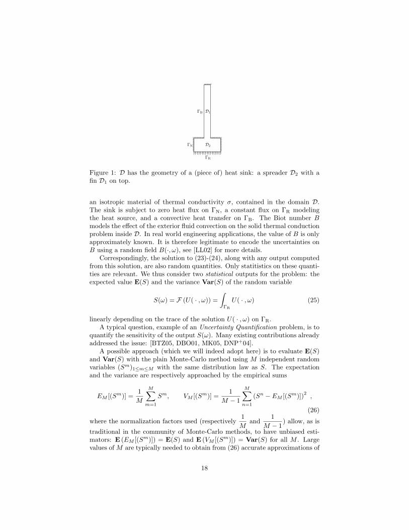
D2

D1ΓB

ΓN

ΓR

Figure 1: D has the geometry of a (piece of) heat sink: a spreader D2 with afin D1 on top.

an isotropic material of thermal conductivity σ, contained in the domain D.The sink is subject to zero heat flux on ΓN, a constant flux on ΓR modelingthe heat source, and a convective heat transfer on ΓB. The Biot number Bmodels the effect of the exterior fluid convection on the solid thermal conductionproblem inside D. In real world engineering applications, the value of B is onlyapproximately known. It is therefore legitimate to encode the uncertainties onB using a random field B(·, ω), see [LL02] for more details.

Correspondingly, the solution to (23)-(24), along with any output computedfrom this solution, are also random quantities. Only statitistics on these quanti-ties are relevant. We thus consider two statistical outputs for the problem: theexpected value E(S) and the variance Var(S) of the random variable

S(ω) = F (U( · , ω)) =

∫ΓR

U( · , ω) (25)

linearly depending on the trace of the solution U( · , ω) on ΓR.A typical question, example of an Uncertainty Quantification problem, is to

quantify the sensitivity of the output S(ω). Many existing contributions alreadyaddressed the issue: [BTZ05, DBO01, MK05, DNP+04].

A possible approach (which we will indeed adopt here) is to evaluate E(S)and Var(S) with the plain Monte-Carlo method using M independent randomvariables (Sm)1≤m≤M with the same distribution law as S. The expectationand the variance are respectively approached by the empirical sums

EM [(Sm)] =1

M

M∑m=1

Sm, VM [(Sm)] =1

M − 1

M∑n=1

(Sn − EM [(Sm)])2,

(26)

where the normalization factors used (respectively1

Mand

1

M − 1) allow, as is

traditional in the community of Monte-Carlo methods, to have unbiased esti-mators: E (EM [(Sm)]) = E(S) and E (VM [(Sm)]) = Var(S) for all M . Largevalues of M are typically needed to obtain from (26) accurate approximations of

18

E(S) and Var(S). Since, for each m = 1, . . . ,M , a new realization of the ran-dom parameter B is considered and the boundary value problem (23)-(24) hasto be solved, the task is clearly computationally demanding. It is a many-querycontext, appropriate for the application of the RB approach.

3.2 Discretization of the problem

We begin by considering the Karhunen–Loeve (abbreviated as KL) expansion

B(x, ω) = bG(x) + b

K∑k=1

Φk(x) Yk(ω) (27)

of the coefficient B(x, ω) (see [Kar46, Loe78, ST06]). In (27), K denotes the(possibly infinite) rank of the covariance operator for B(·, ω), which has eigen-vectors (Φk)1≤k≤K and eigenvalues (λk)1≤k≤K (sorted in decreasing order). Therandom variables (Yk)1≤k≤K are mutually uncorrelated in L2

P(Ω) with zero mean,

G is supposed to be normalized∫∂D G = 1 and b =

∫ΩdP(ω)

∫∂D B(·, ω) is a

fixed intensity factor.Based on (27), we introduce the deterministic function

b(x, y) = bG(x) + b

K∑k=1

Φk(x)yk (28)

defined for almost all x ∈ ∂D and all y ∈ Λy ⊂ RK, where Λy denotes the rangeof the sequence Y = (Yk)1≤k≤K of random variables appearing in (27). Noticethat B(x, ω) = b(x, y(ω)).

It is next useful to consider, for any positive integer K ≤ K, truncated ver-sions of the expansions above, and to define, with obvious notation, UK(·, ω) asthe solution to the problem (23)-(24) where B(·, ω) is replaced by the truncatedKL expansion BK(·, ω) at order K. Similarly, for all yK ∈ Λy, uK( · ; yK) isdefined as the solution to −div

(A(x)∇uK(x; yK)

)= 0 , ∀x ∈ D ,

n(x) ·A(x)∇uK(x; yK) + bK(x, yK)uK(x; yK) = g(x) , ∀x ∈ ∂D,(29)

where bK is the K-truncated sum (28).For a given integer K ≤ K, we approximate the random variable S(ω) by

SK(ω) := F (UK(·, ω)) where UK(·, ω) ≡ uK(·;Y K(ω)), and the statistical out-puts E(SK) and Var(SK) by the empirical sums

EM [(SmK )] =1

M

M∑m=1

SmK , VM [(SmK )] =1

M − 1

M∑n=1

(SnK − EM [(SmK )])2,

(30)usingM independent realizations of the random vector Y K . In practice, uK(·;Y Km )is approached using, say, a finite element approximation uK,N ( · ;Y Km ) with

19

N 1 degrees of freedom. Repeating the task for M realizations of the K-dimensional random vector Y K may be overwhelming, and this is where the RBapproach comes into the picture. We now present the application of the RBapproach to solve problem (29), parametrized by yK ∈ Λy.

In echo to our presentation of Section 2, note that problem (29) is affine inthe input parameter yK thanks to the KL expansion (28) of b, which decouplesthe dependence on x and the other variables. To use the RB approach for thisproblem, we consider S in (30) as the output of the problem, the parameterbeing yK (this parameter takes the values Y K,m, m ∈ 1, . . . ,M being therealization number of Y K) and, as will become clear below, the offline stage isstandard. On the other hand, in the online stage, the a posteriori estimation iscompleted to take into account the truncation error in K in (28).

Before we turn to this, we emphasize that we have performed above anapproximation of the coefficient b, since we have truncated its KL expansion.The corresponding error should be estimated. In addition, the problem (29)after truncation might be ill-posed, even though the original problem (23)-(24)is well posed. To avoid any corresponding pathological issue, we consider astochastic coefficient b having a KL expansion (28) that is positive for anytruncation order K (which is a sufficient condition to ensure the well-posednessof (23)-(24)), and which converges absolutely a.e. in ∂D when K → K. Forthis purpose, (i) we require for k = 1, . . . ,K a uniform bound ‖Φk‖L∞(ΓB) ≤ φ,

(ii) we set Yk := Υ√λkZk with independent random variables Zk uniformly

distributed in the range (−√

3,√

3), Υ being a positive coefficient, and (iii)

we also ask∑Kk=1

√λk < ∞. Note that, if K = ∞, condition (iii) imposes a

sufficiently fast decay of the eigenvalues λk while k increases. We will see inSection 3.4 that this fast decay is also important for the practical success of ourRB approach. Of course, (i)-(ii)-(iii) are arbitrary conditions that we imposefor simplicity. Alternative settings are possible.

3.3 Reduced-Basis ingredients

We know from Section 2 that two essential ingredients in the RB method are an aposteriori estimator and a greedy selection procedure. Like in most applicationsof the RB method, both ingredients have to be adapted to the specificities ofthe present context.

As mentioned above, the statistical outputs (30) require new a posterioriestimators. Moreover, the statistical outputs can only be computed after Mqueries Y Km , m = 1, . . . ,M , in the parameter yK , so these new a posterioriestimators cannot be used in the offline step.

The global error consists of two, independent contributions: the first one isrelated to the RB approximation, the second one is related to the truncation ofthe KL expansion.

In the greedy algorithm, we use a standard a posteriori estimation |SmK,N −SmK,N ,N | ≤ ∆s

N,K(Y Km ) for the error between the finite element approximation

SmK,N := F(uK,N (·;Y Km )) and the RB approximation SmK,N ,N := F(uK,N ,N (·;Y Km ))

20

of SmK at a fixed truncation order K, for any realization Y Km ∈ Λy. This is classi-cal [Boy08, NVP05, RHP] and similar to our example of Section 2, see [BBM+09]for details. Note however that the coercivity constant of the bilinear form forthe variational formulation

Find u(·; yK) ∈ H1(D) s.t.∫Dσ∇u(·; yK) · ∇v +

∫ΓB

b(·, yK)u(·; yK)v =

∫ΓR

g v, ∀ v ∈ H1(D) (31)

of problem (29) depends on K. To avoid the additional computation of thecoercivity constant for each K, we impose b(x, yK) ≥ bG(x)/2, for all x ∈ ΓB ,and thus get a uniform lower bound for the coercivity constant. In practice, thisimposes a limit 0 < Υ ≤ Υmax on the intensity factor in the ranges of the randomvariables Yk, thus on the random fluctuations of the stochastic coefficient, whereΥmax is fixed for all K ∈ 0, . . . ,K

Let us now discuss the online a posteriori error estimation. As for thetruncation error, an a posteriori estimation |SmN − SmK,N | = |F(uN ( · ;Y Km )) −F(uK,N ( · ;Y Km ))| ≤ ∆t

N,K(Y Km ) is derived in [BBM+09]. The error estima-

tors ∆sN,K(Y Km ) and ∆t

N,K(Y Km ), respectively for the RB approximation andthe truncation, are eventually combined for m = 1, . . . ,M to yield global errorbounds in the Monte-Carlo estimations of the statistical outputs: |EM [(SmK,N ,N )]−EM [(SmN )]| ≤ ∆E((SmK,N ,N )) and |VM [(SmK,N ,N )]−VM [(SmN )]| ≤ ∆V ((SmK,N ,N )).The control of the truncation error may be used to improve the performance ofthe reduced basis method. In particular, if the truncation error happens to betoo small compared to the RB approximation error, the truncation rank K maybe reduced.

3.4 Numerical results

Our numerical simulations presented in [BBM+09] are performed on the steadyheat conduction problem (23)-(24) inside the T-shaped heat sink D ⊂ D1 ∪D2 pictured in Fig. 1. The heat sink comprises a 2 × 1 rectangular substrate(spreader) D2 ≡ (−1, 1)× (0, 1) and a 0.5× 4 thermal fin D1 ≡ (−0.25, 0.25)×(1, 5) on top. The diffusion coefficient is piecewise constant, σ = 1D1

+ σ0 1D2,

where 1Di of course denotes the characteristic function of domain Di (i = 1, 2).The finite element approximation is computed using quadratic finite elements ona regular mesh, with N = 6 882 degrees of freedom. The thermal coefficient isσ0 = 2.0. To construct the random input field b(·, ω), we consider the covariancefunction Covar(b(x, ω)b(y, ω)) = (bΥ)2 exp(−(x − y)2/δ2) for b = 0.5, Υ =0.058, and a correlation length δ = 0.5. We perform its KL expansion andkeep only the largest K = 25 terms. We then fix G(x) ≡ 1 and the variablesYk(ω), 1 ≤ k ≤ K, as independent, uniformly distributed random variables.This defines b(·, ω) as the right-hand side of (27).

After computing the reduced basis offline with our RB greedy algorithmon a trial sample of size |Λtrial| = 10 000, the global approximation error in theoutput Monte-Carlo sums EM [(SmK,N ,N )] and VM [(SmK,N ,N )] decays very fast (in

21

2 4 6 8 10 12 1410

−3

10−2

10−1

100

101

N

Δo E

[sN

,K](2,0

.5)

K = 5K = 10K = 15K = 20

2 4 6 8 10 12 1410

−4

10−3

10−2

10−1

100

N

Δo V

[sN

,K](2,0

.5)

K = 5K = 10K = 15K = 20

Figure 2: Global error bounds for the RB approximation error and the KLtruncation error of the output expectation (top: ∆E((SmK,N ,N ))) and of theoutput variance (bottom: ∆V ((SmK,N ,N ))), as functions of the size N = 2, . . . , 14of the reduced basis, at different truncation orders K = 5, 10, 15, 20.

22

fact, exponentially) with the size N = 1, . . . , 14 of the reduced basis, see Fig. 2with K = 20. Note that M = 10 000 for the Monte-Carlo sums. We would alsolike to mention that these reduced bases have actually been obtained lettingvarying not only the parameter Y K , but also additional parameters (namelythe diffusion coefficient σ and the mean b of the Biot number) but this doesnot influence qualitatively the results presented here, and we omit this technicalissue for simplicity (see [BBM+09] for more details).

It is observed that the global approximation error for truncated problemsat a fixed order K and for various N (the size of the reduced basis) is quicklydominated by the truncation error. More precisely, beyond a critical valueN ≥ Ncrit(K), where Ncrit(K) is increasing with K, the global approximationerror becomes constant. Notice that the approximation error is estimated asusual by a posteriori estimation techniques.

When K is infinite (or finite but huge), the control of the KL truncation errormay be difficult. This is a general issue for problems involving a decompositionof the stochastic coefficient. Our RB approach is still efficient in some regimeswith large K, but not all. In particular, a fast decay of the ranges of theparameters (yk)1≤k≤K facilitates the exploration of Λy by the greedy algorithm,which allows in return to treat large K when the eigenvalues λk decay sufficientlyfast with k.

In [BBM+09], we have decreased the correlation length to δ = 0.2 and couldtreat up to K = 45 parameters, obtaining the results in a total computationaltime still fifty times as short as for direct finite element computations.

4 Variance Reduction using an RB approach

In this section, we present a variance reduction technique based upon an RBapproach, which has been proposed recently in [BL09]. In short, the RB ap-proximation is used as a control variate to reduce the variance of the originalMonte-Carlo calculations.

4.1 Setting of the problem

Suppose we need to compute repeatedly, for many values of the parameter λ ∈ Λ,the Monte-Carlo approximation (using an empirical mean) of the expectationE(Zλ) of a functional

Zλ = gλ(XλT )−

∫ T

0

fλ(s,Xλs ) ds (32)

of the solutions(Xλt , t ∈ [0, T ]

)to the Stochastic Differential Equation (SDE)

Xλt = x+

∫ t

0

bλ(s,Xλs ) ds+

∫ t

0

σλ(s,Xλs )dBs, (33)

where(Bt ∈ Rd, t ∈ [0, T ]

)is a d-dimensional standard Brownian motion. The

parameter λ parametrizes the functions gλ, fλ, bλ and σλ. In (33), we assume

23

bλ and σλ allow for the Ito processes(Xλt ∈ Rd, t ∈ [0, T ]

)to be well defined, for

every λ ∈ Λ. Notice that we have supplied the equation with the deterministicinitial condition Xλ

0 = x ∈ Rd. In addition, fλ and gλ are also assumed smooth,such that Zλ ∈ L2(Ω). Recall that a symbolic concise notation for (33) is

dXλt = bλ(t,Xλ

t ) dt+ σλ(t,Xλt ) dBt with Xλ

0 = x.

Such parametrized problems are encountered in numerous applications, suchas the calibration of the volatility in finance, or the molecular simulation ofBrownian particles in materials science. For the applications in finance, E(Zλ)is typically the price of an European option in the Black-Scholes model, andλ enters the diffusion term (the latter being called the volatility in this con-text). The calibration of the volatility consists in optimizing λ so that theprices observed on the market are close to the prices predicted by the model.Any optimization procedure requires the evaluation of E(Zλ) for many valuesof λ. On the other hand, the typical application we have in mind in materi-als science is related to polymeric fluids modelling. There, E(Zλ) is a stresstensor which enters the classical momentum conservation equation on velocityand pressure, and Xλ

t is a vector describing the configuration of the polymerchain, which evolves according to an overdamped Langevin equation, namely astochastic differential equation such as (33). In this context, λ is typically thegradient of the velocity field surrounding the polymer chain at a given point inthe fluid domain. The parameter λ enters the drift coefficient bλ. The com-putation of the stress tensor has to be performed for each time step, and formany points in the fluid domain, which again defined a many-query context,well adapted to the RB approach. For more details on these two applications,we refer to [BL09].

We consider the general form (32)–(33) of the problem and as output the

Monte-Carlo estimation EM[(Zλm)] = 1M

∑Mm=1 Z

λm parametrized by λ ∈ Λ,

where we recall (Zλm) denotes i.i.d. random variables with the same law asZλ. These random variables are build in practice by considering a collectionof realizations of (33), each one driven by a Brownian motion independentfrom the others. In view of the Central Limit Theorem, the rate at whichthe Monte-Carlo approximation EM[(Zλm)] approaches its limit E(Zλ) is givenby 1√

M, the prefactor being proportional to the variance of Zλ. A standard

approach for reducing the amount of computations is therefore variance re-duction [Aro04, MO95, OvdBH97, BP99, HDH64, MT06]. We focus on oneparticular variance reduction technique: the control variate method. It consistsin introducing a so called control variate Y λ ∈ L2(Ω), assumed centered herefor simplicity:

E(Y λ) = 0,

and in considering the equality:

E(Zλ) = E(Zλ − Y λ).

The expectation E(Zλ − Y λ) is approximated by Monte-Carlo estimations EM[(Zλm−Y λm)] which hopefully have, for a well chosen Y λ, a smaller statistical error than

24

direct Monte-Carlo estimations EM[(Zλm)] of E(Zλ). More precisely, Y λ is ex-pected to be chosen so that Var(Zλ) Var(Zλ − Y λ). The central limittheorem yields

EM [(Zλm − Y λm)] :=1

M

M∑m=1

(Zλm − Y λm)P−a.s.−−−−→M→∞

E(Zλ − Y λ), (34)

where the error is controlled by confidence intervals, in turns functions of thevariance of the random variable at hand. The empirical variance

VarM((Zλm − Y λm)

):=

1

M − 1

M∑n=1

(Zλn − Y λn − EM ((Zλm − Y λm))

)2(35)

which, as M → ∞, converges to Var(Zλ), yields a computable error bound.The Central Limit Theorem indeed states that: for all a > 0,

P

(∣∣E(Zλ − Y λ)− EM((Zλm − Y λm)

)∣∣ ≤ a√VarM ((Zλm − Y λm))

M

)−−−−→M→∞

∫ a

−a

e−x2/2

√2π

dx .

(36)Evaluating the empirical variance (35) is therefore an ingredient in Monte-Carlocomputations, similar to what a posteriori estimates are for a deterministicproblem.

Of course, the ideal control variate is, ∀λ ∈ Λ:

Y λ = Zλ −E(Zλ) , (37)

since then, Var(Zλ − Y λ

)= 0. This is however not a practical control vari-

ate since E(Zλ) itself, the quantity we are trying to evaluate, is necessary tocompute (37). Ito calculus shows that the optimal control variate (37) alsowrites:

Y λ =

∫ T

0

∇uλ(s,Xλs ) · σλ(s,Xλ

s )dBs, (38)

where uλ(t, y) ∈ C1([0, T ], C2(Rd)

)satisfies the backward Kolmogorov equa-

tion: ∂tu

λ + bλ · ∇uλ +1

2σλ(σλ)T : ∇2uλ = fλ ,

uλ(T, ·) = gλ(·).(39)

Even using this reformulation, the choice (37) is impractical since solving thepartial differential equation (39) is at least as difficult as computing E(Zλ). Wewill however explain now that both ”impractical” approaches above may givebirth to a practical variance reduction method, when they are combined with aRB type approximation.

Loosely speaking, the idea consists in: (i) in the offline stage, compute fineapproximations of E(Zλ) or respectively uλ for some appropriate values of λ, inorder to obtain fine approximations of the optimal control variate Y λ (at thosevalues) and (ii) in the online stage, for a new parameter λ, use as a controlvariate the best linear combination of the variables built offline.

25

4.2 Two algorithms for variance reduction by the RB ap-proach

Using suitable time discretization methods [KP00], realizations of the stochasticprocess (33) and the corresponding functional (32) can be computed for anyλ ∈ Λ, as precisely as needed. Leaving aside all technicalities related to timediscretization, we thus focus on the Monte Carlo discretization.

We construct two algorithms, which can be outlined as follows.Algorithm 1 (based on formulation (37)):

• Offline stage: Build an appropriate set of values λ1, . . . , λN and, con-currently, for each λ ∈ λ1, . . . , λN compute an accurate approximationEMlarge

[(Zλm)] of E(Zλ) (for a very large number Mlarge of realizations).At the end of the offline step, accurate approximations

Y λ = Zλ − EMlarge[Zλm]

of the optimal control variate Y λ are at hand. The set of values λ1, . . . , λNis chosen in order to ensure the maximal variance reduction in the forth-coming online computations (see below for more details).

• Online stage: For any λ ∈ Λ, compute a control variate Y λN for the Monte-Carlo estimation of E(Zλ) as a linear combination of

(Yi = Y λi)1≤i≤N .

Algorithm 2 (based on formulation (38)):

• Offline stage: Build an appropriate set of values λ1, . . . , λN and, con-currently, for each λ ∈ λ1, . . . , λN, compute an accurate approximationuλ of uλ, by solving the partial differential equation (39). The set of valuesλ1, . . . , λN is chosen in order to ensure the maximal variance reductionin the forthcoming online computations (see below for more details).

• Online stage: For any λ ∈ Λ, compute a control variate Y λN for the Monte-Carlo estimation of E(Zλ) as a linear combination of(

Yi =

∫ T

0

∇uλi(s,Xλs ) · σλ(s,Xλ

s )dBs

)1≤i≤N

.

In both algorithms, we denote by Y λN the control variate built online as a linearcombinations of the Yi’s, the lowerscript index N emphasizing that the ap-proximation is computed on a basis with N elements. An important practicalingredient in both algorithms is to use for the computation of Zλ the exact sameBrownian motions as those used to build the control variates.

The construction of set of values λ ∈ λ1, . . . , λN in the offline stage ofboth algorithms is done using a greedy algorithm similar to those considered in

26

the preceeding sections. The only difference is that the error estimator used isthe empirical variance. Before entering that, we need to make precise how thelinear combinations are built online, since this linear combination constructionis also used offline to choose the λi’s.

The online stage of both algorithms 1 and 2 follow the same line: for a givenparameter value λ ∈ Λ, a control variate Y λN for Zλ is built as an appropriatelinear combination of the control variates (Yi)1≤i≤N (obtained from the offlinecomputations). The criterium used to select this appropriate combination isbased on a minimization of the variance:

Y λN =

N∑n=1

α∗n Yn, (40)

where

(α∗n)1≤n≤N = arg min(αn)1≤n≤N∈RN

Var

(Zλ −

N∑n=1

αnYn

). (41)

In practice the variance in (41) is of course replaced by its empirical approx-imation VarMsmall

. Notice that we have an error estimate of the Monte Carlo

approximation by considering VarMsmall

(Zλ − Y λN

). It is easy to check that

the least squares problem (41) is computationally inexpensive to solve since itamounts to solving a linear N ×N system, with N small. More precisely, thislinear system writes:

CMsmallα∗ = bMsmall

where α∗ here denotes the vector with components α∗n, CMsmallis a matrix with

(i, j)-th entryCovMsmall

(Yi,m, Yj,m)

and bMsmallis a vecteur with j-th component

CovMsmall(Zλm, Yj,m)

where for two collections of random variables Um and Vm,

CovM (Um, Vm) =1

M

M∑m=1

UmVm −(

1

M

M∑m=1

Um

)(1

M

M∑m=1

Vm

).

In summary, the computational complexity of one online evaluation is the sum ofthe computational cost of the construction of bMsmall

(wich scales like NMsmall),and of the resolution of the linear system (which scales like N2 for Algorithm 1since the SVD decomposion of CMsmall

may be precomputed offline, and scaleslike N3 for Algorithm 2, since the whole matrix CMsmall

has to be recomputedfor each new value of λ).

The greedy algorithms used in the offline stages follow the same line as inthe classical RB approach. More precisely, for Algorithm 1, the offline stage

27

writes: Let λ1 ∈ Λtrial be already chosen and compute EMlarge(Zλ1). Then, for

i = 1, . . . , N−1, for all λ ∈ Λtrial, compute Y λi and inexpensive approximations:

Ei(λ) := EMsmall(Zλ − Y λi ) for E(Zλ) ,

εi(λ) := VarMsmall

(Zλ − Y λi

)for Var

(Zλ − Y λi

).

Select λi+1 ∈ argmaxλ∈Λtrial\λj ,j=1,...,i

εi(λ), and compute EMlarge(Zλi+1).

In practice, the number N is determined such that εN (λN+1) ≤ ε, for a giventhreshold ε. The greedy procedure for Algorithm 2 is similar.

4.3 Reduced-Basis ingredients

The algorithms presented above to build a control variate using a reduced basisshare many features with the classical RB approach. The approach follows atwo-stage offline / online strategy. The reduced basis is built using snapshots(namely solutions for well chosen values of the parameters). An inexpensiveerror estimator is used both in the offline stage to build the reduced basis in thegreedy algorithm, and in the online stage to check that the variance reductionis correct for new values of the parameters. The construction of the linearcombinations for the control variates is based on a minimization principle, whichis reminiscent of the Galerkin procedure (3).

The practical efficiency observed on specific examples is similar for the twoalgorithms. They both satisfactorily reduce variance. Compared to the plainMonte Carlo method without variance reduction, the variance is divided atleast by a factor 102, and typically by a factor 104. Algorithm 2 appears tobe computationally much more demanding than Algorithm 1 and less general,since it requires the computation (and the storage) of an approximation of thesolution to the backward Kolmogorov equation (39) for a few values of theparameter. In particular, Algorithm 2 seems impractical for high dimensionalproblems (Xλ

t ∈ Rd with d large). On the other hand, Algorithm 2 seems tobe more robust with respect to the choice of Λtrial: it yields good variancereduction even for large variations of the parameter λ, in the online stage. Werefer to [BL09] for more details.

Notice also that Algorithm 1 is not restricted to a random variable Zλ that isdefined as a functional of a solution to a SDE. The approach can be generalizedto any parametrized random variables, as long as there is a natural methodto generate correlated samples for various values of the parameter. A naturalsetting for such a situation is the computation of a quantity E(gλ(X)) for arandom variable X with given arbitrary law, independent of the parameter λ.In such a situation, it is easy to generate correlated samples by using the samerealizations of the random variable X for various values of the parameter λ.

28

4.4 Numerical Results

The numerical results shown on Figure 3 are taken from [BL09] and relate to thesecond application mentioned in the introduction, namely multiscale models forpolymeric fluids (see [LL07] for a general introduction). In this context, the non-Newtonian stress tensor is defined by the Kramers formula as an expectationE(Zλ) of the random variable:

Zλ = XλT ⊗ F (Xλ

T ) , (42)

where Xλt is a vector modelling the conformation of the polymer chain. The

latter evolves according to an overdamped Langevin equation:

dXλt =

(λXλ

t − F (Xλt ))dt+ dBt. (43)

Equation (43) holds at each position of the fluid domain, the parameter λ ∈Rd×d (d = 2 or 3) being the local instantaneous value of the velocity gradientfield at the position considered. The evolution of the ”end-to-end vector” Xλ

t

is governed by three forces: a hydrodynamic force λXλt , Brownian collisions

Bt against the solvent molecules, and an entropic force F (Xλt ) specific to the

polymer molecule. Typically, this entropic force reads either F (Xλt ) = Xλ

t (for

the Hookean dumbbells), or F (Xλt ) =

Xλt1−|Xλt |2/b

(for the Finitely-Extensible

Nonlinear Elastic (FENE) dumbells, assuming |Xλt | <

√b).

The numerical simulations of the flow evolution of a polymeric fluid usingsuch a model typically consist, on many successive time slots [nT, (n+ 1)T ], oftwo steps: (i) the computation of (43), for a given gradient velocity field λ, atmany points of the fluid domain (think of the nodes of a finite element mesh)and (ii) the computation of a new velocity gradient field in the fluid domain,for a given value of the non-Newtonian stress tensor, by solving the classicalmomentum and mass conservation equations, we omit here for brevity. Thus,E(Zλ) has to be computed for many values λ corresponding to many spatialpositions and many possible velocity fields at each such positions in the fluiddomain.

In the numerical simulations of Figure 3, the SDE (43) for FENE dumbbellswhen d = 2 is discretized with the Euler-Maruyama scheme using 100 iterationswith a constant time step ∆t = 10−2 starting from a deterministic initial con-dition x = (1, 1). Reflecting boundary conditions are imposed on the boundaryof the ball with radius

√b. For b = 16 and |Λtrial| = 100 trial parameter values

randomly chosen in the cubic range Λ = [−1, 1]3 (the traceless matrix λ has en-

tries (λ11 = −λ22, λ12, λ21)), a greedy algorithm is used to incrementally selectN = 20 parameter values after solving |Λtrial| = 100 least-squares problems (41)(with Msmall = 1000) at each step of the greedy algorithm (one for each of thetrial parameter values λ ∈ Λtrial). Then, the N = 20 selected parameter valuesare used online for variance reduction of a test sample of |Λtest| = 1000 randomparameter values.

The variance reduction obtained online by Algorithm 1 withMlarge = 100Msmall

is very interesting, of about 4 orders of magnitude. For the Algorithm 2, we

29

use the exact solution uλ to the Kolmogorov backward equation for Hookeandumbells as an approximation to uλ solution to (39). This also yields satisfy-ing variance reduction though apparently not as good as in Algorithm 1. Asmentioned above, Algorithm 2 is computationally more demanding but seemsto be slightly more robust than Algorithm 1 (namely when some online sampletest Λtestwide uniformly distributed in [−2, 2]3 extrapolates the trial sample usedoffline, see Fig. 3).

0 2 4 6 8 10 12 14 16 18 20-10

10

-810

-610

-410

-210

0 2 4 6 8 10 12 14 16 18 20-10

10

-810

-610

-410

-210

0 2 4 6 8 10 12 14 16 18 20-10

10

-810

-610

-410

-210

0 2 4 6 8 10 12 14 16 18 20-10

10

-810

-610

-410

-210

Figure 3: Algorithm 1 (left) and 2 (right) for FENE model with b = 16. Thex-axis is the size N of the reduced basis. We represent the minimum +, mean× and maximum of VarM [Zλ − Y λN ]/EM [Zλ − Y λN ]2 over online test samplesΛtest ⊂ Λ (top) and Λtestwide ⊃ Λ (bottom) of parameters.

Our numerical tests, although preliminary, already show that the reiteratedcomputations of parametrized Monte-Carlo estimations seem to be a promisingopportunity of applications for RB approaches. More generally, even if RBapproaches may not be accurate enough for some applications, they may beseen as good methods to obtain first estimates, which can then be used toconstruct more refined approximations (using variance reduction as mentionedhere, or maybe preconditionning based on the coarse-grained RB model). Thisis perhaps the most important conclusion of the work described in this section.

30

5 Perspectives

The standard RB method has proved numerically efficient and reliable at reduc-ing the cost of computations for the approximation of solutions to parametrizedboundary value problems in numerous benchmark many-query frameworks. Theseaccomplishments claim for a wider use of the RB method in more realistic set-tings, and even suggest that some RB ideas could still be extended in numerousmany-query frameworks yet largely unexplored, including the stochastic context.The success of the RB approach in parametrized boundary value problems isonly understood precisely from a mathematical perspective in a few very simplecases. This should motivate further theoretical investigations.

In this section, we discuss various tracks for the development of reducedbasis techniques, both from a methodological viewpoint and in terms of possibleapplications, with a focus on the stochatic context presented above.

5.1 A posteriori estimation in the stochastic context

We already emphasized that a crucial ingredient in the RB approach is an ac-curate and fast a posteriori estimator for the approximation error between twolevels of discretization (the initially discretized, non-reduced one and the re-duced one). Therefore, before everything, the future developments of the RBmethod should definitely concentrate on improving the a posteriori estimators.In particular, for the new contexts of application that are stochastic, there seemsto remain some room for a yet better understanding of the a posteriori errorestimation. More precisely, the best way to evaluate the reduction error whenthe Galerkin approximations (used by deterministic applications) are replacedwith Monte-Carlo approximations is still unclear. For a first application ofthe RB ideas to stochastic applications, we have used confidence intervals asa probabilistic measure of the Monte-Carlo approximation error. These confi-dence intervals are only reliable in the limit of infinitely many realizations of therandom variables. But there are other possibilities, like using non-asymptoticupper-bounds for the error which hold whatever the number of realizations (us-ing for example Chebyshev inequalities or Berry-Esseen type bounds). In ad-dition, the numerical evaluation of the variance is not obvious either. Untilnow, we have used Monte-Carlo estimators, but there exist other possibilitiestoo which could be faster or more accurate and should thus be tested. Finally,another idea related to the method presented in Section 4 would be to mimickthe usual RB approach, by considering that the reference result is the one ob-tained with Mlarge realizations, and to develop a posteriori error bounds withrespect to this reference solution (using for example conditional expectationswith respect to the Mlarge realizations).

5.2 Affine decompositions and the stochastic context

As explained above, the RB approach is to date only efficient at yielding compu-tational reductions in the context of affine parametrization. However, as shown

31

in the previous sections, a many-query parametrized framework is not necessar-ily parametrized in an affine way. So one may have to pretreat the problem inorder to transform it as the limit of a sequence of affinely-parametrized problems.It would thus be interesting to derive rapidly convergent affine approximationsfor non-affine problems. For instance, the Karhunen-Loeve decomposition usedto pretreat a random field entering a partial differential equation as a coefficientmay converge too slowly for an efficient use of the RB method applied to trun-cated decompositions, in the context of random fields with small correlationlengths. One should then look for other possible affine representation of therandom variations in the input coefficient. Now, there are many possible tracksto solve this problem, like projecting the random field on a well-chosen basisfor the oscillation modes of the coefficient for instance (many possible basesmay exist for the realizations of the random field, depending on its regularity),interpolating (recall the so-called empirical interpolation with magic points),etc.

5.3 Application to Bayesian statistics

A context where the RB ideas could be applied is Bayesian statistics where themany-query parametrized framework is naturally encountered. We now makethis more precise by presenting a specific example that would be well-suited forthe application of Algorithm 1 in Section 4.

Let us consider, for given values of a parameter µ1, an ensemble of observa-tions (xµ1

i )1≤i≤Nµ1data. Following the Bayesian framework, a stochastic model is

proposed to model the observation: the quantities (xµ1

i )1≤i≤Nµ1dataare supposed

to form a set of independent and identically distributed samples following a givendistribution parametrized by another set of parameters µ2 (think for exampleof a mixture of Gaussians, µ2 being then the triplets of weights, means andvariances of each Gaussians). The Bayesian approach then consists in postulat-ing a so-called prior distribution (with a probability density function denotedPrior(µ2) below) on the parameters µ2, and to compute the so-called posteriordistribution, namely the distribution of µ2 given the observations (with a prob-ability density function denoted Π

(µ2|(xµ1

i )1≤i≤Nµ1data

)below). Of course, the

posterior distribution for µ2 is expected to depend on µ1: for each µ1, the aimis thus to sample the probability measure Π

(µ2|(xµ1

i )1≤i≤Nµ1data

)dµ2, with

Π(µ2|(xµ1

i )1≤i≤Nµ1data

)= (Zµ1)−1Π

((xµ1

i )1≤i≤Nµ1data|µ2

)Prior(µ2)

where Zµ1 is the normalization constant, and Π((xµ1

i )1≤i≤Nµ1data|µ2

)is the so-

called likelihood function, namely the probability density function of the obser-vations given the datas. One possible technique to sample the posterior distri-bution consists in drawing samples according to the prior distribution, and toweight each of them using the likelihood function, which depends on µ1. Withsuch a sampling technique, it is easy to draw correlated samples for variousvalues of µ1. Following Algorithm 1 in Section 4, it would thus be possible tobuild a reduced basis based on the sampling of the posterior distribution for

32

some selected values of µ1 (offline stage), in order to reduce the variance forthe sampling of the posterior distribution for other generic values of µ1 (onlinestage).

5.4 Relation to functional quantization

One computationally demanding stochastic context that defines a many-queryframework is the approximation of the solution to a parametrized stochasticdifferential equation, for many values of the parameter. We already mentionedapplications in finance and rheology in Section 4, where a variance reductiontechnique based on RB was proposed. Another idea consists in first computingprecise discretizations of a few processes at some well-chosen parameter values,and then to use them for a faster computation of an approximation of theprocesses for other values of the parameter.

Functional quantization is an approach that has independently been devel-oped along this line, see for instance [LuPa02, PP05]. The idea of quantizationis to approximate a square-integrable random variable with values in a Hilbertspace by a random variable that takes a finite number of values, in an optimalway. In its simplest form, quantization deals with Gaussian random variableswith values in Rd, but it can also be applied to Gaussian processes. The nu-merical approach developped in [PS08] to solve stochastic differential equationsis to first quantize the Brownian motion, and then to solve a collection of ordi-nary differential equations in order to recover approximations of the solutionsto the stochastic differential equations as linear combinations of the ordinarydifferential equations solutions. Clearly, this approach for the discretization ofstochastic differential equations has intimate connection with a RB approach.In particular, the computations are split into two parts: an offline step, whichis computationally expensive, to quantize the Brownian motion, and then anonline step to solve ordinary differential equations rather than stochastic differ-ential equations.

In a setting where the stochastic differential equations are parametrized, anatural similar idea would be to quantize the solution to the stochastic differen-tial equations for a few values of the parameter, and next to build the solutionto the stochastic differential equation for another value of the parameter as alinear combination of these precomputed solutions.

References

[AO00] M. Ainsworth and J. T. Oden. A Posteriori Error Estimation inFinite Element Analysis. Wiley-Interscience, 2000.

[ASB78] B. O. Almroth, P. Stern, and F. A. Brogan. Automatic choiceof global shape functions in structural analysis. AIAA Journal,16:525–528, 1978.

33

[Aro04] B. Arouna. Robbins-monroe algorithms and variance reduction infinance. The Journal of Computational Finance, 7(2):35–62, 2004.

[BNT07] I. Babuska, F. Nobile, and R. Tempone. A stochastic collocationmethod for elliptic partial differential equations with random inputdata. SIAM Journal on Numerical Analysis, 45(3):1005–1034, 2007.

[BTZ05] I. Babuska, R. Tempone, and G. Zouraris. Solving elliptic bound-ary value problems with uncertain coefficients by the finite elementmethod: the stochastic formulation. Comput. Meth. Appl. Mech.Eng., 194:1251–1294, 2005.

[BNMP04] M. Barrault, N. C. Nguyen, Y. Maday, and A. T. Patera. An“empirical interpolation” method: Application to efficient reduced-basis discretization of partial differential equations. C. R. Acad.Sci. Paris, Serie I., 339:667–672, 2004.

[BR95] A. Barrett and G. Reddien. On the reduced basis method. Z.Angew. Math. Mech., 75(7):543–549, 1995.

[BR01] R. Becker and R. Rannacher. An optimal control approach to a pos-teriori error estimation in finite element methods. Acta Numerica,37:1–225, 2001.

[BP99] J. Bonvin and M. Picasso. Variance reduction methods forCONNFFESSIT-like simulations. J. Non-Newtonian Fluid Mech.,84:191–215, 1999.

[Boy08] S. Boyaval. Reduced-basis approach for homogenization beyond theperiodic setting. SIAM Multiscale Modeling & Simulation, 7(1):466–494, 2008.

[Boy09] S. Boyaval. Mathematical modeling and simulation for materialscience. PhD thesis, Universite Paris Est, 2009.

[BBM+09] S. Boyaval, C. Le Bris, Y. Maday, N.C. Nguyen, and A.T. Patera.A reduced basis approach for variational problems with stochasticparameters: Application to heat conduction with variable Robin co-efficient. Computer Methods in Applied Mechanics and Engineering,198(41–44):3187–3206, 2009.

[BL09] S. Boyaval and T. Lelievre. A variance reduction method forparametrized stochastic differential equations using the reduced ba-sis paradigm. In Pingwen Zhang, editor, Accepted for publicationin Communication in Mathematical Sciences, volume Special Issue“Mathematical Issues on Complex Fluids”, 2009.

[BMPPT10] A. Buffa, Y. Maday, A.T. Patera, C. Prud’homme and G. Turinici.A priori convergence of the greedy algorithm for the parametrizedreduced basis. Submitted to M2AN (Math. Model. Numer. Anal.).

34

[BGL06] J. Burkardt, M. D. Gunzburger, and H. C. Lee. POD and CVT-based reduced order modeling of Navier-Stokes flows. Comp. Meth.Applied Mech., 196:337–355, 2006.

[Cia78] Ph. Ciarlet. The Finite Element Method for Elliptic Problems.North-Holland, Amsterdam, 1978.

[CDD] A. Cohen, R. A. Devore, and W. Dahmen. Personal communication.

[DBO01] M.K. Deb, I.M. Babuska, and J.T. Oden. Solution of stochastic par-tial differential equations using galerkin finite element techniques.Comp. Meth. Appl. Mech. Engrg., 190(48):6359–6372, 2001.

[DNP+04] B.J. Debusschere, H.N. Najm, P.P. Pebay, O.M. Knio, R.G.Ghanem, and O.P. Le Maıtre. Numerical challenges in the useof polynomial chaos representations for stochastic processes. SIAMJournal on Scientific Computing, 26(2):698–719, 2004.

[Dep09] S. Deparis. Reduced basis error bound computation of parameter-dependent Navier-Stokes equations by the natural norm approach.SIAM Journal of Numerical Analysis, 46(4):2039–2067, 2009.

[Dev93] R. A. Devore. Constructive approximation. Acta Numerica, 7:51–150, 1993.

[FR83] J. P. Fink and W. C. Rheinboldt. On the error behavior of thereduced basis technique for nonlinear finite element approximations.Z. Angew. Math. Mech., 63(1):21–28, 1983.

[FM71] R. L. Fox and H. Miura. An approximate analysis technique fordesign calculations. AIAA Journal, 9(1):177–179, 1971.

[GS91] R. G. Ghanem and P. D. Spanos. Stochastic Finite Elements: ASpectral Approach. Springer Verlag, New York edition, 1991. Re-vised First Dover Edition, 2003.

[GMNP07] M. A. Grepl, Y. Maday, N. C. Nguyen, and A. T. Patera. Efficientreduced-basis treatment of nonaffine and nonlinear partial differen-tial equations. M2AN (Math. Model. Numer. Anal.), 41(2):575–605,2007. (doi: 10.1051/m2an:2007031).

[GP05] M. A. Grepl and A. T. Patera. A Posteriori error boundsfor reduced-basis approximations of parametrized parabolic par-tial differential equations. M2AN (Math. Model. Numer. Anal.),39(1):157–181, 2005.

[GvL96] G. Golub and C. van Loan. Matrix computations, third edition. TheJohns Hopkins University Press, London, 1996.

[Gun89] M. D. Gunzburger. Finite Element Methods for Viscous Incom-pressible Flows. Academic Press, 1989.

35

[HO08a] B. Haasdonk and M. Ohlberger. Reduced basis method for finitevolume approximations of parametrized linear evolution equations.M2AN (Math. Model. Numer. Anal.), 42(3):277–302, 2008.

[HO08b] B. Haasdonk and M. Ohlberger. Adaptive Basis Enrichment forthe Reduced Basis Method Applied to Finite Volume Schemes. InProc. 5th International Symposium on Finite Volumes for ComplexApplications, June 08-13, 2008, Aussois, France. 471–478, 2008.

[HDH64] J. Hammersley and eds. D. Handscomb. Monte Carlo Methods.Chapman and Hall Ltd, London, 1964.

[HKY+09] D.B.P. Huynh, D.J. Knezevic, Y.Chen, J.S. Hesthaven, and A. T.Patera. A natural-norm successive constraint method for inf-suplower bounds. Computer Methods in Applied Mechanics and En-gineering, 2009. submitted, preprint version available on URLhttp://augustine.mit.edu/methodology/papers/.

[HRSP07] D.B.P. Huynh, G. Rozza, S. Sen, and A.T. Patera. A successive con-straint linear optimization method for lower bounds of parametriccoercivity and inf-sup stability constants. C. R. Math. Acad. Sci.Paris, 345:473–478, 2007.

[HP07] D. B. P. Huynh and A. T. Patera. Reduced-basis approxima-tion and a posteriori error estimation for stress intensity fac-tors. Int. J. Num. Meth. Eng., 72(10):1219–1259, 2007. (doi:10.1002/nme.2090).

[Kar46] K. Karhunen. Zur spektraltheorie stochastischer prozesse. AnnalesAcademiae Scientiarum Fennicae, 37, 1946.

[KP00] P. Kloeden and E. Platen. Numerical Solution of Stochastic Differ-ential Equations. Springer, 2000.

[KP09] D.J. Knezevic and A.T. Patera. A certified reduced basis methodfor the Fokker-Planck equation of dilute polymeric fluids: FENEdumbbells in extensional flow. submitted to SIAM Journal of Sci-entific Computing, 2009.

[KV02] K. Kunisch and S. Volkwein. Galerkin proper orthogonal decompo-sition methods for a general equation in fluid dynamics. SIAM J.Num. Analysis, 40(2):492–515, 2002.

[LB05] C. Le Bris. Systemes multi-echelles : Modelisation & simulation,volume 47 of Mathematiques & applications. Springer, 2005.

[LL07] C. Le Bris and T. Lelievre. Multiscale modelling of complex fluids:A mathematical initiation. In Multiscale Modeling and Simula-tion in Science Series, B. Engquist, P. Lotstedt, O. Runborg, eds.,LNCSE 66, Springer, p. 49-138, 2009.

36

[LL02] J. H. Lienhard IV and J. H. Lienhard V. A Heat Transfer Textbook.Phlogiston Press, Cambridge, Mass., 2002.

[Lin91] M. Y. Lin Lee. Estimation of the error in the reduced-basis methodsolution of differential algebraic equations. SIAM Journal of Nu-merical Analysis, 28:512–528, 1991.

[Loe78] M. Loeve. Probability Theory, volume I-II. Springer, New York,1978.

[LuPa02] H. Luschy and G. Pages Functional quantization of Gaussian pro-cesses J. Funct. Anal., 196:486–531, 2002.

[Mad06] Y. Maday. Reduced–basis method for the rapid and reliable solu-tion of partial differential equations. In Proceedings of InternationalConference of Mathematicians, Madrid. European MathematicalSociety Eds., 2006.

[MNPP09] Y. Maday, N. C. Nguyen, A. T. Patera, and G. Pau. A general,multipurpose interpolation procedure: the magic points. Commu-nications on Pure and Applied Analysis, 8(1):383–404, 2009.

[MPT02a] Y. Maday, A. T. Patera, and G. Turinici. A Priori convergencetheory for reduced-basis approximations of single-parameter ellipticpartial differential equations. Journal of Scientific Computing, 17(1-4):437–446, 2002.

[MPT02b] Y. Maday, A.T. Patera, and G. Turinici. Global a priori convergencetheory for reduced-basis approximations of single-parameter sym-metric coercive elliptic partial differential equations. C. R. Acad.Sci. Paris, Ser. I, 335(3):289–294, 2002.

[MK05] H.G. Matthies and A. Keese. Galerkin methods for linear and non-linear elliptic stochastic pdes. Comput. Meth. Appl. Mech. Eng.,194:1295–1331, 2005.

[MO95] M. Melchior and H.C. Ottinger. Variance reduced simulations ofstochastic differential equations. J. Chem. Phys., 103:9506–9509,1995.

[MT06] G.N. Milstein and M.V. Tretyakov. Practical variance reductionvia regression for simulating diffusions. Technical Report MA-06-19, School of Mathematics and Computer Science, University ofLeicester, 2006.

[Nag79] D. A. Nagy. Modal representation of geometrically nonlinear be-haviour by the finite element method. Computers and Structures,10:683–688, 1979.

37

[Nguyen07] N. C. Nguyen. A multiscale reduced-basis method for parametrizedelliptic partial differential equations with multiple scales. Journalof Computational Physics, 227:9807–9822, 2007.

[Noo81] A. K. Noor. Recent advances in reduction methods for nonlinearproblems. Comput. Struct., 13:31–44, 1981.

[Noo82] A. K. Noor. On making large nonlinear problems small. Comp.Meth. Appl. Mech. Engrg., 34:955–985, 1982.

[Noor84] A. K. Noor, C. D. Balch, and M. A. Shibut. Reduction methodsfor non-linear steady-state thermal analysis. Int. J. Num. Meth.Engrg., 20:1323–1348, 1984.

[NP80] A. K. Noor and J. M. Peters. Reduced basis technique for nonlinearanalysis of structures. AIAA Journal, 18(4):455–462, 1980.

[NP83a] A. K. Noor and J. M. Peters. Multiple-parameter reduced basistechnique for bifurcation and post-buckling analysis of compositeplates. Int. J. Num. Meth. Engrg., 19:1783–1803, 1983.

[NP83b] A. K. Noor and J. M. Peters. Recent advances in reduction methodsfor instability analysis of structures. Comput. Struct., 16:67–80,1983.

[NPA84] A. K. Noor, J. M. Peters, and C. M. Andersen. Mixed models andreduction techniques for large-rotation nonlinear problems. Comp.Meth. Appl. Mech. Engrg., 44:67–89, 1984.

[New96] A. J. Newman. Model reduction via the Karhunen-Loeve expan-sion part i: an exposition. Technical Report Institute for SystemResearch University of Maryland, (96-322), 1996.

[New94] N. J. Newton. Variance reduction for simulated diffusions. SIAMJ. Appl. Math., 54(6):1780–1805, 1994.

[NRHP09] N. C. Nguyen, G. Rozza, D. B. P. Huynh, and A. T Patera. Re-duced basis approximation and a posteriori error estimation forparametrized parabolic pdes; application to real-time bayesian pa-rameter estimation. In Biegler, Biros, Ghattas, Heinkenschloss,Keyes, Mallick, Tenorio, van Bloemen Waanders, and Willcox, edi-tors, Computational Methods for Large Scale Inverse Problems andUncertainty Quantification, John Wiley & Sons, UK, 2009.

[NRP08] N. C. Nguyen, G. Rozza, and A. T. Patera. Reduced basis approx-imation and a posteriori error estimation for the time-dependentviscous burgers equation. Calcolo, 46(3):157–185, 2009.

[NVP05] N. C. Nguyen, K. Veroy, and A.T. Patera. Certified real-time solu-tion of parametrized partial differential equations, pages 1523–1558.Springer, 2005. (S. Yip, editor).

38

[Nou07] A. Nouy. A generalized spectral decomposition technique to solvea class of linear stochastic partial differential equations. ComputerMethods in Applied Mechanics and Engineering, 196(45-48):4521–4537, 2007.

[Nou08] A. Nouy. Generalized spectral decomposition method for solvingstochastic finite element equations: Invariant subspace problem anddedicated algorithms. Computer Methods in Applied Mechanics andEngineering, 197(51-52):4718–4736, 2008.

[OvdBH97] H. C. Ottinger, B. H. A. A. van den Brule, and M. A. Hulsen. Brow-nian configuration fields and variance reduced CONNFFESSIT. J.Non-Newtonian Fluid Mech., 70(30):255 – 261, 1997.

[PP05] G. Pages and J. Printems. Functional quantization for numericswith an application to option pricing. Monte Carlo Methods andAppl., 11(4):407–446, 2005.

[PS08] G. Pages and A. Sellami. Convergence of multi-dimensional quan-tized SDE’s. http://arxiv.org/abs/0801.0726, 2008.

[PR07a] A. T. Patera and E. M. Rønquist. Reduced basis approximationsand a posteriori error estimation for a Boltzmann model. Com-puter Methods in Applied Mechanics and Engineering, 196:2925–2942, 2007.

[PR07b] A. T. Patera and G. Rozza. Reduced Basis Approximation and APosteriori Error Estimation for Parametrized Partial DifferentialEquations. Copyright MIT, 2006–2007. To appear in MIT Pap-palardo Monographs in Mechanical Engineering.

[Pet89] J. S. Peterson. The reduced basis method for incompressible viscousflow calculations. SIAM J. Sci. Stat. Comput., 10(4):777–786, 1989.

[Pin85] A. Pinkus. n-Widths in Approximation Theory. Springer, 1985.

[Por85] T. A. Porsching. Estimation of the error in the reduced basismethod solution of nonlinear equations. Mathematics of Compu-tation, 45(172):487–496, 1985.

[Por87] T. A. Porsching and M. Y. Lin Lee. The reduced-basis methodfor initial value problems. SIAM Journal of Numerical Analysis,24:1277–1287, 1987.

[PRV+02] C. Prud’homme, D. Rovas, K. Veroy, Y. Maday, A. T. Patera, andG. Turinici. Reliable real-time solution of parametrized partial dif-ferential equations: Reduced-basis output bounds methods. Journalof Fluids Engineering, 124(1):70–80, 2002.

39

[Qua09] A. Quarteroni. Numerical Models for Differential Problems, vol-ume 2. Springer, 2009.

[Rhe81] W. C. Rheinboldt. Numerical analysis of continuation methods fornonlinear structural problems. Computers and Structures, 13(1-3):103–113, 1981.

[Rhe93] W. C. Rheinboldt. On the theory and error estimation of the re-duced basis method for multi-parameter problems. Nonlinear Anal-ysis, Theory, Methods and Applications, 21(11):849–858, 1993.

[RHP] G. Rozza, D.B.P. Huynh, and A. T. Patera. Reduced basis approxi-mation and a posteriori error estimation for affinely parametrized el-liptic coercive partial differential equations — application to trans-port and continuum mechanics. Arch. Comput. Methods Eng. toappear September 2008.

[ST06] C. Schwab and R.A. Todor. Karhunen-loeve approximation of ran-dom fields by generalized fast multipole methods. Journal of Com-putational Physics, 217(1):100–122, 2006.

[Sen08] S. Sen. Reduced-basis approximation and a posteriori error esti-mation for many-parameter heat conduction problems. NumericalHeat Transfer, Part B: Fundamentals, 54(5), 2008.

[SVH+06] S. Sen, K. Veroy, D. B. P. Huynh, S. Deparis, N. C. Nguyen, andA. T. Patera. “Natural norm” a posteriori error estimators for re-duced basis approximations. Journal of Computational Physics,217:37–62, 2006.

[SF73] G. Strang and G. J. Fix. An Analysis of the Finite Element Method.Prentice-Hall, 1973.

[V.N08] V.N.Temlyakov. Nonlinear methods of approximation. Foundationsof Computational Mathematics, 3:33–107, 2008.

[VPRP03] K. Veroy, C. Prud’homme, D. V. Rovas, and A. T. Patera. A Poste-riori error bounds for reduced-basis approximation of parametrizednoncoercive and nonlinear elliptic partial differential equations. InProceedings of the 16th AIAA Computational Fluid Dynamics Con-ference, 2003. Paper 2003-3847.

[VRP02] K. Veroy, D. Rovas, and A. T. Patera. A Posteriori error estimationfor reduced-basis approximation of parametrized elliptic coercivepartial differential equations: “convex inverse” bound conditioners.ESAIM: Control, Optimization and Calculus of Variations, 8:1007–1028, 2002.

40